washington forest biomass supply assessment
TRANSCRIPT

Washington Forest Biomass Assessment Report 2012/03/13 Page 1
WASHINGTON FOREST BIOMASS SUPPLY ASSESSMENT
This Report was prepared for Washington Department of Natural Resources by University of Washington, College of the Environment, School of Environmental and Forest Sciences and TSS Consultants with financial support from USDA Forest Service
March 13, 2012
University of Washington College of the Environment
School of Environmental and Forest Sciences

Washington Forest Biomass Assessment Report 2012/03/13 Page 2

Washington Forest Biomass Assessment Report 2012/03/13 Page 3
Washington Forest Biomass Supply Assessment
Acknowledgements:
We wish to thank Peter Goldmark, Commissioner of Public Lands and Aaron Everett, State Forester, for securing Forest Service funds that were awarded to complete the project. The project was made possible with a grant from the USDA Forest Service State and Private Forestry. We thank the many people who contributed their time and insights throughout the assessment. In particular we thank Aaron Everett, Craig Partridge, Rachael Jamison and Jeff Linquist from the Washington Department of Natural Resources, attendees at 4 public meetings, those who took our calls and answered our emails in our pursuit to clarify information. We are also indebted to the technical review team for their insights and constructive comments submitted on the draft versions of the report.
Project Team:
John Perez-Garcia, PI (UW)
Elaine Oneil, Project Manager (UW)
Todd Hansen, Project Manager (TSS Consultants)
Tad Mason (TSS Consultants)
James McCarter (UW)
Luke Rogers (UW)
Andrew Cooke (UW)
Jeff Comnick (UW)
Matt McLaughlin (UW)
Contact Information: WADNR: Rachael Jamison, Project Manager, ([email protected])
UW/School of Forest Resources: John Perez-Garcia, ([email protected])
TSS Consultants: Todd Hansen, ([email protected])

Washington Forest Biomass Assessment Report 2012/03/13 Page 4
Federal Civil Rights
In accordance with Federal law and U.S. Department of Agriculture policy, DNR does not discriminate on the basis of race, color, national origin, sex, age or disability. However, should a person wish to file a discrimination complaint, please write to:
USDA, Director Office of Civil Rights Room 326-W, Whitten Building 1400 Independence Avenue SW Washington D.C. 20250-9410 or call 202.720.5964 (voice and TDD).
USDA is an equal opportunity provider and employer.

Washington Forest Biomass Assessment Report 2012/03/13 Page 5
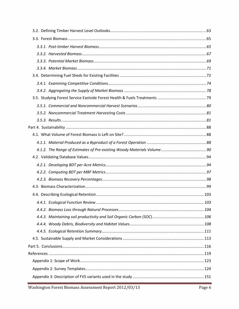
Contents List of Tables ................................................................................................................................................. 8
List of Figures ................................................................................................................................................ 9
Executive Summary ..................................................................................................................................... 11
Part 1. Introduction to the Study Report ................................................................................................... 18
1.1. Study Tasks ...................................................................................................................................... 19
1.2. Study Approach Outline .................................................................................................................. 20
1.3. Navigating the Report ..................................................................................................................... 22
Part 2. Assessment Methods ..................................................................................................................... 25
2.1. Simulating Forest Inventory ............................................................................................................ 25
2.1.1. Acquiring and Processing Inventory Data ................................................................................ 25
2.1.2. Modeling Used with the GNN Databases ................................................................................. 26
2.1.3. Creating Tree Lists to Determine Biomass Volumes ................................................................. 26
2.2. Calculating Biomass for the Forest Inventory ................................................................................. 26
2.2.1. Selecting a Biomass Equation .................................................................................................. 26
2.2.2. Outlining the Process of Biomass Calculations ........................................................................ 29
2.2.3. Developing the Harvest Scenario Matrix .................................................................................. 29
2.2.4. Calculating Post-Timber Harvest Biomass ............................................................................... 31
2.2.5. Determining Harvest Configuration Constraints ...................................................................... 33
2.2.6. Calculating Harvested Biomass ................................................................................................ 37
2.2.7. Determining Potential Market Biomass Operability Constraints ............................................. 38
2.2.8. Calculating Potential Market Biomass ..................................................................................... 41
2.2.9. Using Cost Assumptions to Determine Market Biomass .......................................................... 42
2.2.10. Cost Center Definitions ........................................................................................................... 43
2.2.11. Calculating the Residual Value to the Landowner ................................................................. 44
2.2.12. Conducting Network Analysis ................................................................................................ 46
2.2.13. Calculating Market Biomass .................................................................................................. 47
2.2.14. Calculating the Volume of Biomass Left Behind ..................................................................... 48
2.3. Biomass Database Design ............................................................................................................... 50
2.3.1. The Washington State Biomass Database ............................................................................... 50
2.3.2. The Harvest Scenarios .............................................................................................................. 52
2.3.3. Additional Database Information Layers ................................................................................. 54
Part 3. Results ............................................................................................................................................ 62
3.1. The Study Area ................................................................................................................................ 62
Washington Forest Biomass Assessment Report 2012/03/13 Page 6
3.2. Defining Timber Harvest Level Outlooks ......................................................................................... 63
3.3. Forest Biomass ................................................................................................................................ 65
3.3.1. Post-timber Harvest Biomass ................................................................................................... 65
3.3.2. Harvested Biomass ................................................................................................................... 67
3.3.3. Potential Market Biomass ........................................................................................................ 69
3.3.4. Market Biomass ....................................................................................................................... 71
3.4. Determining Fuel Sheds for Existing Facilities ................................................................................ 72
3.4.1. Examining Competitive Conditions........................................................................................... 74
3.4.2. Aggregating the Supply of Market Biomass ............................................................................ 78
3.5. Studying Forest Service Eastside Forest Health & Fuels Treatments ............................................. 79
3.5.1. Commercial and Noncommercial Harvest Scenarios ............................................................... 80
3.5.2. Noncommercial Treatment Harvesting Costs .......................................................................... 81
3.5.3. Results ...................................................................................................................................... 81
Part 4. Sustainability .................................................................................................................................. 88
4.1. What Volume of Forest Biomass Is Left on Site? ............................................................................ 88
4.1.1. Material Produced as a Byproduct of a Forest Operation ....................................................... 88
4.1.2. The Range of Estimates of Pre-existing Woody Materials Volume .......................................... 90
4.2. Validating Database Values ............................................................................................................. 94
4.2.1. Developing BDT per Acre Metrics ............................................................................................. 94
4.2.2. Computing BDT per MBF Metrics ............................................................................................. 97
4.2.3. Biomass Recovery Percentages ................................................................................................ 98
4.3. Biomass Characterization ................................................................................................................ 99
4.4. Describing Ecological Retention .................................................................................................... 103
4.4.1. Ecological Function Review .................................................................................................... 103
4.4.2. Biomass Loss through Natural Processes ............................................................................... 104
4.4.3. Maintaining soil productivity and Soil Organic Carbon (SOC) ................................................ 106
4.4.4. Woody Debris, Biodiversity and Habitat Values ..................................................................... 108
4.4.5. Ecological Retention Summary............................................................................................... 111
4.5. Sustainable Supply and Market Considerations ........................................................................... 113
Part 5. Conclusions ................................................................................................................................... 116
References ................................................................................................................................................ 119
Appendix 1: Scope of Work ................................................................................................................... 123
Appendix 2: Survey Templates.............................................................................................................. 124
Appendix 3: Description of FVS variants used in the study .................................................................. 151

Washington Forest Biomass Assessment Report 2012/03/13 Page 7
Appendix 4: Biomass Equations used in the study ............................................................................... 152
Appendix 5: Harvest Scenario Matrix (Harvest-Management Scenarios Draft 20110125.xls) ............ 153
Appendix 6: Biomass Tables.................................................................................................................. 159
Appendix 7: Fuelsheds for Existing Facilities ........................................................................................ 160
Appendix 8: Pre-existing Woody Biomass by Major Wildlife Habitat Type .......................................... 175

Washington Forest Biomass Assessment Report 2012/03/13 Page 8
List of Tables Table 1. Definitions of biomass established for this report ....................................................................... 24 Table 2. Summary of harvest and forest operation scenarios ................................................................... 29 Table 3. Eastside Harvest Levels ................................................................................................................ 32 Table 4. Westside Harvest Levels ............................................................................................................... 32 Table 5. Equipment cost per hour .............................................................................................................. 43 Table 6. Harvest Targets for State lands in Klickitat County ...................................................................... 52 Table 7. Treatment allocations for State lands on an acreage basis ......................................................... 52 Table 8. Percentage of acres being pre-commercially thinned as modeled in the database .................... 53 Table 9. Example biomass collection percentages based on topography, owner class, forest ecosystem
and SVA ............................................................................................................................. 53 Table 10. Owner class description and codes ............................................................................................ 55 Table 11. Parcel management classes ....................................................................................................... 56 Table 12. Federal and Tribal Riparian Management Classes ..................................................................... 57 Table 13. Stream and Body of Water Buffer Distances ............................................................................. 58 Table 14. Wetland Buffer Distances ........................................................................................................... 58 Table 15. Reserved and unreserved acres by owner class......................................................................... 59 Table 16. Assignment of pre-2010 harvest to management classes and zones ........................................ 60 Table 17. BDT per MBF metrics using post-timber harvest biomass volume ............................................ 66 Table 18. BDT per MBF metrics using harvested biomass volume ............................................................ 69 Table 19. BDT per MBF metrics using potential market biomass volume ................................................. 71 Table 20. Three cost levels for set-up, processing and loading, and hauling used to determine market
biomass volumes .............................................................................................................. 71 Table 21. Biomass in BDT under the three scenarios and according to biomass definition. ..................... 85 Table 22. The distribution of biomass in million BDT according to the naming convention used in this
study (see Figure 2) ........................................................................................................... 89 Table 23. DecAid data summarized by Wildlife Habitat Types of Washington State for open canopy
conditions ......................................................................................................................... 91 Table 24. Range of downed wood for forested stands in the open canopy condition class ..................... 91 Table 25. Average and 80% tolerance level of BDT per acre of pre-existing downed wood >5” in
diameter by forest ecosystem type .................................................................................. 92 Table 26. Per acre biomass estimates calculated using the database. ...................................................... 95 Table 27. The distribution of the difference between post-timber harvest biomass and potential market
biomass (Biomass retained on site as a byproduct of a forest operation) ....................... 96 Table 28. BDT per MBF values for harvested biomass calculated from the biomass database ................ 97 Table 29. BDT per MBF values for region forest type calculated from field surveys and interviews ........ 98 Table 30. Diameter distribution of dispersed biomass ONRC study – Olympic Peninsula ...................... 100 Table 31. Diameter distribution of post-timber operation biomass Okanogan – Wenatchee National
Forest Fuel Survey ........................................................................................................... 101 Table 32. Diameter distribution of pre-existing biomass Olympic National Forest Fuel Survey ............. 101 Table 33. Westside physical characteristics of processed and unprocessed materials. .......................... 102 Table 34. Eastside physical characteristics of processed and unprocessed materials. ........................... 103 Table 35. Estimated consumption of forest biomass by existing facilities .............................................. 114

Washington Forest Biomass Assessment Report 2012/03/13 Page 9
List of Figures Figure 1. Task Relationships with Main Outputs........................................................................................ 21 Figure 2. Flow of biomass produced as a byproduct of a forest operation from forest to market ........... 22 Figure 3. Biomass calculated in the study included the tree stem, top, bark, branches and needles
(leaves), and stump and roots. ......................................................................................... 27 Figure 4. Alternative computational methods considered for the study to determine the volume of
biomass in the stem for Douglas fir stem biomass. .......................................................... 28 Figure 5. Harvest system distribution weighted by volume for ownership and forest type (Source: study
survey data) ...................................................................................................................... 37 Figure 6. Post-timber harvest biomass conversion into harvest biomass pathway .................................. 38 Figure 7. Recovery percent based upon operability conditions DF = Douglas fir type, RA = hardwood
type, PP = Ponderosa pine type, TF/MC = True fir, mixed conifer type, WH = western hemlock type. (Source: Study survey data). ..................................................................... 41
Figure 8. Harvested biomass conversion into potential market biomass or residual potential market biomass pathway .............................................................................................................. 42
Figure 9. Price and tonnage of market biomass relationship (First number is the haul rate; second number is the processing cost; third number is the move-in costs. 160/20@100 uses $160 haul rate, $20 processing rate and $100 move-in cost) .......................................... 45
Figure 10. Example concentric service area rings around a facility for a one-hour drive time. ................ 47 Figure 11. Potential market biomass conversion into market biomass pathway ...................................... 48 Figure 12. The volume of biomass that was left behind (indicated by boldface type) defined by three
sources of residual biomass left on site as a result of a forest operation plus pre-existing woody material. ................................................................................................................ 49
Figure 13. Combined "segments" in the database .................................................................................... 51 Figure 14. Left to Right: BLM, County, and DNR source data for Mason County ...................................... 54 Figure 15. Final parcel data for Mason County, from multiple data sources ............................................ 55 Figure 16. Reserved (red) and unreserved areas in Washington ............................................................... 60 Figure 17. Source road network datasets (left) and combined final road network (right) ....................... 61 Figure 18. Forest Ecosystem Types by Stumpage Valuation Areas ............................................................ 62 Figure 19. Harvest outlooks studied in the assessment ............................................................................ 63 Figure 20. Aggressive harvest outlook by ownership ................................................................................ 64 Figure 21. Mid-range harvest outlook by ownership ................................................................................. 64 Figure 22. Conservative harvest outlook by ownership ............................................................................ 64 Figure 23. Post-timber harvest biomass by ownership under the aggressive harvest outlook ................ 65 Figure 24. Post-timber harvest biomass by ownership under the mid-range harvest outlook ................. 65 Figure 25. Post-timber harvest biomass by ownership under the conservative harvest outlook ............. 66 Figure 26. Harvested biomass volume by ownership under the aggressive harvest outlook ................... 67 Figure 27. Harvested biomass volume by ownership under the mid-range harvest outlook ................... 68 Figure 28. Harvested biomass volume by ownership under the conservative harvest outlook ............... 68 Figure 29. Potential market biomass volume by ownership under the aggressive harvest outlook......... 69 Figure 30. Potential market biomass volume by ownership under the mid-range harvest outlook ......... 70 Figure 31. Potential market biomass volume by ownership under the conservative harvest outlook ..... 70 Figure 32. The expansion of a facility’s fuel shed as market price increased under medium cost level for
2010 .................................................................................................................................. 73 Figure 33. Market biomass fuelsheds under low cost at varying market prices for all exisiting facilities . 75 Figure 34. Market biomass fuelsheds under medium cost at varying market prices for all exisiting
facilities ............................................................................................................................. 76 Figure 35. Market biomass fuelsheds under high cost at varying market prices for all exisiting facilities 77

Washington Forest Biomass Assessment Report 2012/03/13 Page 10
Figure 36. Supply curves for existing facilities by ID number showing different quantities availability with price changes .................................................................................................................... 78
Figure 37. Aggregate supply in 2015 using medium cost level at different harvest outlook levels .......... 79 Figure 38. Aggregate supply in 2015 using Midrange harvest outlook at different cost levels ................ 79 Figure 39. Forest Service production of Post-Timber Harvest Biomass under three levels of harvest
activity under a light thinning regime. .............................................................................. 82 Figure 40. Forest Service production of Harvested Biomass under three levels of harvest activity under a
light thinning regime. ........................................................................................................ 82 Figure 41. Forest Service production of Potential market biomass under three levels of harvest activity
under a light thinning regime. .......................................................................................... 83 Figure 42. Forest Service production of Post-Timber Harvest Biomass under three levels of harvest
activity under a heavy thinning regime. ........................................................................... 84 Figure 43. Forest Service production of Harvested Biomass under three levels of harvest activity under a
heavy thinning regime. ..................................................................................................... 84 Figure 44. Forest Service production of Potential market biomass under three levels of harvest activity
under a light thinning regime. .......................................................................................... 85 Figure 45. Market biomass supply from national forests in 2015 under the baseline case fpr three cost
scenarios using the light thinning regime. ........................................................................ 86 Figure 46. Market biomass supply from national forests in 2015 under the Increased case fpr three cost
scenarios using the light thinning regime. ........................................................................ 87 Figure 47. Market biomass supply from national forests in 2015 under the Aggressive case for three
cost scenarios using the light thinning regime. ................................................................ 87 Figure 48. Dispersed biomass estimates for the mid-range harvest scenario plus the residual harvested
biomass calculated in the biomass database ................................................................... 93 Figure 49. Minimum of piles and dispersed biomass estimates for the mid-range harvest scenario (does
not include residual market biomass left in piles due to economic constraints) ............. 93 Figure 50. Summary of biomass under the various definitions used in the assessment ........................... 94 Figure 51. Market for biomass with current consumption represented by low and high ranges and
supply represented by medium cost level and midrange harvest outlook for 2010. .... 115

Washington Forest Biomass Assessment Report 2012/03/13 Page 11
Executive Summary The study reports the contributions of forest-based biomass as a byproduct of sustainable forest operations to economic development within economic, technological, and ecological constraints. Three major goals were accomplished with the study. First, an estimate was produced of the volume of forest biomass, stratified by landownership categories, forest ecosystem types, species and location (whether it was removed or retained on site). Producing stratified biomass data led to the development of a spatially explicit biomass database. Second, the study assesses biomass availability based on various cost and price considerations, market prices and calculating residual value to the landowner. Third, public to access the biomass database is provided through the internet via a web-based calculator tool. The research team studied the process of biomass production beginning with a forest harvest operation. The team calculated the volume of biomass at all stages of processing and inferred the contribution it makes to market uses and ecological function when it was retained on site. The study also produced an estimate of pre-existing woody material based on references and studies in existing literature.
The report also studied alternative scenarios regarding fuels treatment and forest health in National Forests in eastern Washington. The scenarios reflected a future that increased the number of acres treated for fuels reduction and forest health reasons, and calculated the volume of biomass produced as a result of these treatments. Figure E.1 shows the allocation of material from a forest harvest operation into merchantable stem volume and biomass starting from left to right. Biomass on a parcel began as the volume of slash that was produced as a byproduct of a forest operation. Biomass was everything generated as part of the timber harvest process including tops, live/dead branches, and foliage, and included breakage and defect associated with stem volume. This biomass was classified as post-timber harvest biomass. Post-timber harvest biomass was then allocated to either potential market or non-market uses. The biomass that was brought to the landing and roadside was calculated and recorded in the biomass database as harvested biomass. The volume that was left scattered in the woods as a product of having been broken off or tops and limbs cut when commercial logs were yarded to the landing was noted as residual harvested biomass. Biomass that reached the landing and roadside was filtered by operability constraints for each ownership and forest type, and became either potential market biomass or residual potential market biomass. The potential market biomass represented the amount that could be potentially loaded onto a truck. The residual potential market biomass was the portion that did not get loaded due to operability constraints (equipment cannot be brought in) or other factors such as landowner preferences (the landowner does not want to sell their biomass). The potential market biomass was the volume that was subject to market valuation and was furthered filtered by economic parameters. Market biomass was the portion of the potential market biomass that actually was loaded on a truck. Some market residual was produced when costs considerations were included. This residual was noted as residual market biomass. The accounting was complete when the volume of biomass reaching the market was recorded.

Washington Forest Biomass Assessment Report 2012/03/13 Page 12
Figure E1. The progression of biomass from forest slash (upper rectangle) to market (lower rectangle). The numbers in boxes represent statewide volume calculated for 2010.
Of nearly 4.4 million bone dry tons (MM BDT) produced by forest operations in 2010, 3 MM BDT were harvested (brought to a landing), and 1.4 MM BDT were retained on site as a byproduct of a forest operation (tops and breakage). The majority of the 1.4 MM BDT of residual harvested biomass was assumed to be left scattered throughout the harvest unit. Of the 3 MM BDT of harvested biomass in 2010, 1.4 MM BDT were potentially marketable. The volume of unmarketable harvested biomass left in piles and at landings was calculated to be 1.6 MM BDT. Of the 1.4 MM BDT of potential market biomass, around 0.6 MM BDT were sold to facilities under 2010 costs and market prices. The amount left in piles at landings due to low market prices amounted to 0.8 MM BDT. Today’s market conditions for biomass, primarily due to low economic activity, restrict the volume of potential market biomass that can reach biomass end users. Under more favorable prices than those observed in 2010, e.g., $100 per BDT (up from $30-65 per BDT in 2010), market biomass could have expanded to 1.3 MM BDT, leaving about 0.1 MM BDT at the roadside.
In addition to the biomass that resulted from a forest operation and that can be marketed, we evaluated woody material that existed prior to the operation. Pre-existing woody material is usually not available as market biomass. Pre-existing woody material was determined by consulting the decayed wood advisor (DecAID, US Forest Service). The range of pre-existing woody material on site ranged from 0 to 7.2 MM BDT when the 80% tolerance limit from DecAID was used (see figure E1). Using the study’s
Post-timber Harvest Biomass 4.4 MM BDT
F
ores
t Ope
ratio
n Pre-existing woody material ranges from 0 to 7.2 MM BDT
Merchantable Stem Volume 7.5 MM BDT
Harvested Biomass 3.0 MM BDT
Potential Market Biomass 1.4 MM BDT
Market Biomass 0.6 – 1.3 MM BDT
Residual Harvested Biomass 1.4 MM BDT
Residual Potential Market Biomass 1.6 MM BDT
Residual Market Biomass 0.1 – 0.8 MM BDT

Washington Forest Biomass Assessment Report 2012/03/13 Page 13
mid-range harvest scenario, the 80% tolerance limit of pre-existing woody material estimates provided by DecAID, and the study’s technical and economic filters that were used to allocate biomass across its different categories, the study team estimated a minimum of 8.6 MM BDT (in 2010) and a maximum of 11 MM BDT (in 2015) of biomass that were left on harvested sites statewide (figure E2). The variability in this total pictured in figure E2 was a mirrored reflection of the mid-range harvest projection used in the study. The mid-range harvest projection was the middle level of three harvest scenarios analyzed in the study. The minimum tonnage reflected low levels of harvested activity, while the maximum tonnage corresponds to the year of highest harvest activity.
Figure E2. The range of material left scattered in a unit.
More importantly, the source of greatest variability in figure E2 was associated with the pre-existing volume of woody material. The study's calculations show that retained woody biomass immediately following a timber harvest will always add to pre-existing levels. Additional biomass produced as a result of a forest operation in piles and at roadside added 2.4 MM BDT for 2010. This value is the sum of residual biomass associated with potential market biomass and market biomass described in figure E1.
Three harvest configurations were developed to assess how the volume of market biomass produced might change under alternative future views of economic activity. A conservative outlook included lowering harvest levels to 2.1 billion board feet (BBF) in 2015. This outlook took the view that the economic conditions observed in 2010 further deteriorated to 2015, reaching a stable level in 2015. A midrange harvest outlook raised 2015 harvest levels to 3 BBF annual in an expected response to an economic recovery, then fluctuated around a narrow band as economic conditions might fluctuate. The aggressive harvest outlook created harvest levels that were much more responsive in the short term, reaching 3.7 BBF in 2015, then falling back slightly to fluctuate around 3.5 BBF (Figure E3). Future levels of harvest are likely to be within the range embodied by these upper and lower outlooks.
-
2
4
6
8
10
12
14
2010 2015 2020 2025 2030
Biom
ass
in m
illio
ns o
f BDT
Pre-Existing up to the80% tolerance level
Residual HarvestedBiomass

Washington Forest Biomass Assessment Report 2012/03/13 Page 14
Figure E3. Three harvest configurations used in the assessment
Figure E4 presents the statewide production of potential market biomass volume by management class for the mid-range timber harvest outlook depicted in figure E3. The majority of the potential market biomass was produced by private landowners. The production of potential market biomass was proportional to the timber harvest level.
Figure E4. Potential market biomass under a midrange harvest outlook
Aggregate supply was defined using a cost model, the residual value to the landowner, competition from nearby facilities that determined where residuals were sent and market prices. The range of production costs for processing and loading biomass was from $16 to $35 per BDT. The range of hourly rates for transporting processed biomass was from $70 to $115 per hour. Finally, moving equipment to the site ranged from $700 to $1100 per operation. Figure E5 reproduces the market supply functions under the three harvest outlook scenarios depicted in figure E3 for 2015, the period when differences in the harvest volume were greatest. Two points are evident from figure E5. First, existing costs and the availability of potential market biomass suggested that biomass sold to facilities could expand with a small increase in market price per ton, e.g., less than $10 per BDT increase. This is indicated in the figure by the flatness of the curve over a large portion of volume. Second, higher harvest levels increased biomass availability by the same proportional increase in harvest volume. This is indicated in the figure
0.00.51.01.52.02.53.03.54.04.5
2010 2015 2020 2025 2030
Mer
chan
tabl
e Ha
rves
t Vo
lum
e (B
BF)
Aggressive
MidRange
Conservative
0.0
0.5
1.0
1.5
2.0
2.5
2010 2015 2020 2025 2030
Pote
ntia
l Mar
ket B
iom
ass
(Mill
ion
BDT)
Tribal
State
Small Private
Other Public
Large Private
Federal

Washington Forest Biomass Assessment Report 2012/03/13 Page 15
by the shifts in the supply curves from the conservative harvest level (left curve) to the aggressive harvest level (right curve). Changes in the assumptions on cost levels (not shown in Figure E5) also affected biomass supply. The changes led to shifts upwards of the curves as assumptions on production cost associated with processing biomass, and hauling it to facilities increased these costs.
Figure E5. Aggregate biomass supply in 2015 associated with varying levels of timber harvest volume estimated at medium production costs
The research team created a database from their calculations (http://wabiomass.cfr.washington.edu/). Metrics produced from data contained in the study database on BDT per thousand board feet (MBF) and BDT per acre were cross-checked with field interviews and secondary sources (table E1). Per acre measures of biomass retained on site were found to be consistent with these field studies and interviews. The values contained in the study’s database appear to be within values needed for ecological functions.
Table E1. Biomass retained on site as a byproduct of a forest operation in BDT per acre. Average vales were weighted by acres.
Federal Large Private Other Public Small Private State Tribal AVERAGE EAST 19.18 22.66 19.69 22.12 23.98 23.43 21.95
DF 16.81 17.21 20.76 22.03 23.22 21.67 20.09 PP 20.02 18.12 15.57 16.36 21.45 20.70 18.68 RA 14.94 - 13.81 11.66 3.49 11.86 TFMC 21.00 28.22 18.87 25.43 27.62 28.75 25.27 WH 18.08 39.90 48.60 32.16 33.23 31.92 30.97
WEST 21.94 32.92 30.66 31.55 36.68 28.35 32.14 DF 21.76 34.40 28.02 32.72 41.36 9.09 32.89 PP 11.45 12.17 8.03 12.90 16.11 15.78 13.85 RA 15.87 32.37 34.15 33.14 32.32 19.51 31.09 TFMC 20.11 34.53 27.36 26.54 34.38 31.61 30.13 WH 29.24 42.47 36.71 38.35 47.99 45.58 41.10
Source: Biomass database. DF, Douglas fir; PP, Ponderosa pine; RA, Red Alder/Hardwoods; TFMC, True fir/Mixed conifers; WH, Western hemlock; OP, other pine.
An assessment of forest health treatments on Forest Service lands in eastern Washington was completed. An aggressive harvest outlook using heavy thinning options was simulated on eastside Forest Service lands and their production to biomass supply noted. Figure E6 illustrates the shift in market supply associated with this aggressive treatment scenario under 3 costs assumptions. Additional
$- $20 $40 $60 $80
$100 $120
0.0 0.5 1.0 1.5 2.0 2.5Mar
ket P
rice
($/B
DT)
Million BDT
Conservative Midrange Aggressive

Washington Forest Biomass Assessment Report 2012/03/13 Page 16
biomass ranged 102,000 BDT to 152,000 BDT at a $100 market price level. Prices of $45 per BDT suggested biomass availability from 7,300 to 93,000 BDT depending on costs.
Figure E6. The shift in aggregate supply when forest health treatments in eastern Washington are implemented on Forest Service lands In 2015
The statewide market biomass supply that can be sustained was also calculated. The sustainable level of biomass was a function the biomass market price. The study team estimated that from 439,000 to 558,000 BDT of biomass were delivered to facilities in 2010. Figure E7 combines the market supply under the medium cost level for 2010 with the estimated range in demand. With market prices slightly higher than current values, the amount of market biomass supplied could double at current timber harvest levels. Potential market biomass was available to meet a doubling of demand. Currently market conditions constrained this material to be retained on site in piles or along roadside. At levels greater than 1 million BDT of market biomass, competition among facilities over the limited amount supplied was evident. At some facilities, there appears to be competitive factors that restrict supplies locally, bidding prices higher. The 2010 market could have sustained the production of 1.3 MM BDT at a price of $100 per BDT.
$-
$20
$40
$60
$80
$100
$120
- 40,000 80,000 120,000 160,000
Mar
ket P
rice/
BDT
BDT
AgressiveLightLow AggressiveLightMed AggressiveLightHigh

Washington Forest Biomass Assessment Report 2012/03/13 Page 17
Figure E7. Market supply and demand In 2010
In general, most forest landowners and land managers indicated that the byproduct of their harvest or treatment operations was piled and burned, remained dispersed throughout the unit, or was hauled back and scattered throughout the unit, if biomass recovery was not a viable option. This response was supported by our database calculations. Our calculations revealed that only 14% of the post-timber harvest biomass was marketed (see figure E1). From interviews, the study team summarized that much of the post-timber harvest material was unanimously characterized as unsuited for current market conditions or material not meeting contract removal specifications. This response reflects merchandizing specifications for local and regional markets, species composition, and access to pulp log or niche product markets (e.g., fuel pellets). Material unsuited for markets typically consists of breakage during harvesting, defect culled during log manufacturing, stumps, undersize stems or top diameter, limbs, twigs and needles or leaves. Stumps are typically not included as recoverable biomass, with some exceptions occurring during road right-of-way construction requiring stump removal. However, including soil or rock material embedded within the roots can contaminate the biomass and increase ash content to unacceptable levels.
While the study did not attempt to sort the type of biomass into categories, such a system may yield significant improvements in recovery metrics. Value-added improvements may be as simple as slight modifications to timber harvest operation protocols, stacking and piling that creates opportunities to extract the higher-valued material or other changes in practices to concentrate the most valued material at roadside. In addition, there is likely to be some production efficiency gains in both harvest configuration and operability if market prices were to increase.
$- $20 $40 $60 $80
$100 $120
0.0 0.5 1.0 1.5
Mar
ket P
rice
($/B
DT)
Million BDT
Low Demand Range Medium Cost Supply 2010
High Demand Range

Washington Forest Biomass Assessment Report 2012/03/13 Page 18
Part 1. Introduction to the Study Report In 2010 the Washington State Department of Natural Resources (DNR) received funding from the USDA Forest Service to assess the sustainable long-term supply of forest biomass that could be made available within the state for energy generation projects. Legislation authorizing DNR to enter into long-term supply contracts for this forest biomass from state-managed trust lands required that prior to exercising the contracting authority, a long-term supply assessment was a necessary prerequisite. A study was also timely to address concerns regarding the sustainability of biomass supply considering ecological considerations, competing uses, economic demand and cost. A contract between the University of Washington’s School of Forest Resources and DNR was signed at the end of 2010, with TSS Consultants acting as a sub-contractor to the University. The report describes the results of an assessment that considered the contributions of biomass produced as a byproduct of forest operations under a range of market conditions within economic, technological, and ecological constraints. The report also studied alternative scenarios regarding fuels treatment and forest health in National Forests in eastern Washington.
The demand for renewable energy and biofuel is expected to rise due to renewable energy portfolio increases and interest in biojet fuels. Forest biomass is viewed as potentially the largest source of non-hydro renewable energy available in Washington State. In addition to electricity, forest biomass can fulfill a unique role as a source of heat, steam, and/or liquid transportation fuels. A critical first step necessary to capitalize on the resource’s potential energy feedstock value was to assess its sustainable supply taking into account economic, ecological and technological limitations.
Biomass is a byproduct of forest operations that include activities related to timber harvest, forest health and fire risk-reduction, and other stand management activities. The study team defined biomass according to its stage of processing. Biomass’s first stage was the residual volume of a timber harvest operation. These operations were modeled using an updated forest inventory to provide the volume of biomass supply. Modeling results were informed by recently conducted field interviews that were used to provide current economic and technological information on biomass recovery. In addition to interviews, the study team used existing growth and yield models with inventory plot data for Washington State and an updated forest landowner database to derive the volume of residuals produced by forest operations. Then the study tracked the volume through a series of value-added processes that eventually led to the amount of biomass sold to energy facilities. This accounting process, from the production of residuals as a byproduct of a forest operation through to the portion that reached the facility’s gate, permitted us to remark about the volume that was left behind, either at the roadside and landings, or scattered throughout the forest site. We compliment these data with estimates of pre-existing downed-woody material found in the literature. Ecological functions dependent on biomass retained on site were researched through a literature review and are discussed in the report.
The report describes two major accomplishments in detail. First we describe the development of a biomass database that is spatially explicit and contains a rich set of alternative forest management operations across the diversity of owner groups and forest types in the state of Washington. The

Washington Forest Biomass Assessment Report 2012/03/13 Page 19
database created for the assessment is accessible through a web-based portal for individual use (http://wabiomass.cfr.washington.edu/). Second, using this database, the study team completed an assessment of the current conditions of forest biomass operations and their sustainable outlook. Since additional biomass recovery might occur should its value rise sufficiently to make removal of greater amounts economically possible, we have also reported results based on alternative economic conditions that reflect an expected increase in demand.
1.1. Study Tasks DNR outlined fourteen points of coverage in the request for proposal. We summarize them here.
3.1.1 Stratify the supply assessment by landownership categories, forest ecosystem type, hardwood and softwood categories, logical supply areas and time periods in decades.
3.1.2 Determine estimated volume of timber harvest residuals left on-site, and estimated volume of residuals removed; and relevant physical characteristics of those timber harvest residuals across logging areas.
3.1.3 Project volumes of biomass that could result from precommercial thinning, forest health and fuel reduction treatments, salvage operations and other origins, if any.
3.1.4 Estimated volume, physical characteristics, and distribution of material, live and dead, under a reasonable range of on-site retention levels, and operational constraints, to protect soil productivity, water quality, fish and wildlife habitat (including species of concern), and other ecological functions.
3.1.5 Estimate the operationally feasible volume, cost, and quality of removed biomass under a range of reasonable scenarios.
3.1.6 Produce an estimate of the cost of various modes and distances of transportation to the given processing facility locations.
3.1.7 Produce an estimate based on currently available information, of a range of the prices in $ per ton for delivered biomass matched to various biomass physical quality characteristics (moisture; content; particle size; impurities; density; etc.).
3.1.8 Produce an estimate of the volume, origins, and physical characteristics of biomass which could be ecologically and economically removed from forest lands in Washington on a long-term sustainable basis,
3.1.9 Break out estimates of biomass by supply tributary areas, landowner category, forest ecosystem type; hardwood and softwood categories, and time period in decades.
3.1.10 Provide estimates by biomass origin (logging residuals; silvicultural; forest health; or fuel reduction treatment; salvage; or other biomass) and landowner category.
3.1.11 Include appropriate sensitivity analysis to show those economic, physical, ecological, or other factors having the greatest influence on the overall supply assessment results.
Washington Forest Biomass Assessment Report 2012/03/13 Page 20
3.1.12 Develop and deliver a biomass supply assessment calculator tool as a separate component.
3.1.13 Describe the approach to gaining detailed data needed to estimate operations and outputs by landowner class, and to estimate volumes of residuals, and thinned or salvaged material using recent published data, where geographically and operationally relevant, or other approaches.
3.1.14 Incorporate the techniques, data, and relevant results of the recent biomass studies.
The request for proposal process resulted in successfully awarding a contract to the University of Washington (UW), as prime contractor, and TSS Consultants, as subcontractors to UW, with the purpose of completing a statewide sustainable forest biomass supply study. The final scope of work is presented in Appendix 1.
1.2. Study Approach Outline Our work plan strategy consisted of (i) building upon the existing Washington State Forestland Database (Rogers and Cooke 2009) that provided a flexible platform for modeling and supply assessment, (ii) utilizing the modeling and assessment expertise at the University of Washington and (iii) capitalizing on TSS Consultant’s capacity to provide technological and economic knowledge of biomass resource collection and utilization alternatives.
DNR’s fourteen points of coverage listed above were viewed as interrelated and, for the large part, inseparable. The study team’s view taken early on was to produce a single integrated document on biomass supply rather than 14 individual pieces. Our study logic and progression is represented in Figure 1. Three major goals were envisioned. First, we would produce an estimate, stratified by landownership categories, forest ecosystem types, species and location (whether it was removed or retained on site), of the volume of forest biomass. The effort behind the production of this stratified biomass data led to the development of a biomass database containing spatially explicit, and appropriately stratified data on the volume of biomass produced by as a byproduct of a forest operation. Second, we would produce an assessment of availability based on various cost and price considerations. The assessment was completed using cost models developed for this work, market prices and residual value to the landowner calculations. Our third goal was to permit the public to access the biomass database through the internet via a webpage.

Washington Forest Biomass Assessment Report 2012/03/13 Page 21
Figure 1. Task Relationships with Main Outputs
Tasks: 3.1.1 – 3.1.4, 3.1.9, 3.1.10
Tasks: 3.1.5 – 3.1.8, 3.1.11
Biomass Supply Assessment Calculator (Task 3.1.12: EFFORT 3)
Major Effort 1
Major Effort 2

Washington Forest Biomass Assessment Report 2012/03/13 Page 22
1.3. Navigating the Report We studied the progression of biomass that begins with a forest operation and finishes at a facility’s gate. We followed this progression noting whether forest biomass remained on site or was removed and used to support economic activity. Figure 2 outlines the progression of biomass that began with a harvest operation, producing post-timber harvest biomass and culminated as market biomass. Residual biomass production occurred at each step of the process. In addition to the residual biomass produced as a byproduct of a forest operation, there existed a range of woody material prior to the forest operation. Table 1 found at the end of the section provides definitions for biomass terms used.
Figure 2. Flow of biomass produced as a byproduct of a forest operation from forest to market
Post-timber harvest biomass was determined using inventory plot data for Washington state, growth and yield models that used the plot data, forest operation behavior and biomass equations, all contained in a newly-developed biomass database. The details of the study methods, models and the database are described in Part 2 of the report.
Post-timber harvest biomass was produced as a byproduct of a forest operation, and was either piled and brought to a roadside (harvested biomass), or remained scattered on site (residual harvested biomass). Equipment configuration and type determined whether post-timber harvest biomass reached the roadside. The study team used field surveys to collect information on the range of harvest configurations that determined whether post-timber harvest biomass became harvested biomass or residual harvested biomass.
Post-timber Harvest Biomass
F
ores
t Ope
ratio
n
Pre-existing woody material
Merchantable Stem Volume
Harvested Biomass
Potential Market Biomass
Market Biomass
Residual Harvested Biomass
Residual Potential Market Biomass
Residual Market Biomass

Washington Forest Biomass Assessment Report 2012/03/13 Page 23
Harvested biomass became either potential market biomass or remained on site as residual potential market biomass due to operability constraints. The biomass left on site in piles or by the roadside consisted of the volume of harvested biomass that was not processed. The potential market biomass represented the portion that could get loaded onto a truck.
Market biomass was the volume loaded onto a truck. It was calculated using a cost and market price assessment. Residual market biomass was the volume left behind due to unfavorable economic conditions.
Residual biomass remaining on site due to harvest configuration constraints (eg. residual harvested biomass), operability constraints (eg. residual potential market biomass) and market constraints (eg. residual market biomass) was in addition to the volume of woody material pre-existing a forest operation. The study team did not analyze the sum of the residual biomass further except to characterize it using information gathered in interviews and from a review of the literature. We noted its role in meeting ecological functions and future market demand, and produced a range of pre-existing volumes found in the literature that was in addition to the residual material produced as a byproduct of a forest operation.
The report explains the methods and constraints used in calculating biomass volumes at each stage of processing in Part 2. It details the biomass accounting framework that begins with a forest operation through its finality at a facility’s gate, remarking on the residual volumes that remained on site. Part 3 presents the assessment findings. The report contains the estimates of biomass stratified by landownership categories, forest ecosystem types, species and location, and provides an assessment of availability based at various cost and price considerations. The study team also reports the results of the effect alternative future views of fuels treatment and forest health conditions can have on biomass availability in Part 3. Part 4 discusses the assessment findings. It presents, first, a comparison of the calculated volumes using the biomass database with the extant literature, second, a presentation of the range of pre-existing downed-woody material likely to be found prior to forest operations, third, a discussion of the importance of ecological retention, and finally, remarks about markets. Part 5 concludes the study.
Washington Forest Biomass Assessment Report 2012/03/13 Page 24
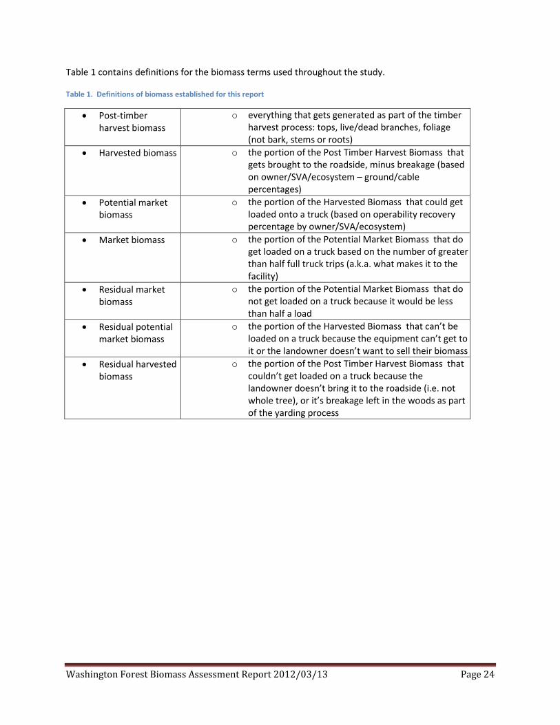
Table 1 contains definitions for the biomass terms used throughout the study.
Table 1. Definitions of biomass established for this report
• Post-timber harvest biomass
o everything that gets generated as part of the timber harvest process: tops, live/dead branches, foliage (not bark, stems or roots)
• Harvested biomass o the portion of the Post Timber Harvest Biomass that gets brought to the roadside, minus breakage (based on owner/SVA/ecosystem – ground/cable percentages)
• Potential market biomass
o the portion of the Harvested Biomass that could get loaded onto a truck (based on operability recovery percentage by owner/SVA/ecosystem)
• Market biomass o the portion of the Potential Market Biomass that do get loaded on a truck based on the number of greater than half full truck trips (a.k.a. what makes it to the facility)
• Residual market biomass
o the portion of the Potential Market Biomass that do not get loaded on a truck because it would be less than half a load
• Residual potential market biomass
o the portion of the Harvested Biomass that can’t be loaded on a truck because the equipment can’t get to it or the landowner doesn’t want to sell their biomass
• Residual harvested biomass
o the portion of the Post Timber Harvest Biomass that couldn’t get loaded on a truck because the landowner doesn’t bring it to the roadside (i.e. not whole tree), or it’s breakage left in the woods as part of the yarding process

Washington Forest Biomass Assessment Report 2012/03/13 Page 25
Part 2. Assessment Methods The assessment was implemented using three basic activities. We used (i) inventory plot data for Washington state, (ii) growth and yield models linked to the plot data and biomass equations for tree components, and (iii) forest operation behavior determined from a survey of land managers to calculate the volume of biomass as the byproduct of forest operations. Once the model simulations were completed, we linked the results to an updated parcel database to extract ownership information and then applied network analysis to complete the transportation assessment. Finally, we examined existing studies and survey responses to validate the calculated volumes of biomass. To these data, we added a range of pre-existing downed-woody material. The following sections describe the process we followed to calculate biomass in its progression from forest slash to market biomass. At the end of each section we summarize the accounting process that occurred from one stage to the next reproducing Figure 2 in greater detail as a guide.
Interviews with logging contractors, biomass processors, hauling contractors and foresters were conducted to establish biomass recovery metrics and processing logistics necessary for collection, processing and transport of biomass feedstock. Not all timber harvest technologies, forest road systems or landscapes (topography) accommodated recovery and transport of biomass feedstock, and the survey and interviews were used to identify those utilization practices that did (See Appendix 2).
Section 2.1 presents the study methods used to create an inventory for Washington state. Section 2.2 presents the calculations carried out to report biomass volumes produced as a byproduct of a forest operation. Section 2.3 describes the database developed to store the volumes of biomass through all its processes.
2.1. Simulating Forest Inventory
2.1.1. Acquiring and Processing Inventory Data Forest inventory data developed by the Landscape Ecology, Modeling, Mapping & Analysis (LEMMA) group located at Oregon State University were used to develop inventory profiles for Washington. The LEMMA project used the Gradient Nearest Neighbor (GNN) method for creating large scale, high resolution spatial maps of vegetation for analysis. Complete coverage of Washington state was provided by using multiple modeling regions from two LEMMA GNN projects: Mapping for Northwest Forest Plan Effectiveness Monitoring (NWFP) and the Interagency Mapping and Assessment Project (IMAP).
We analyzed the spatial information combined from these two projects, and produced 6,085 unique forest class plots (FCID), of which 5,998 are forested. Discussion of some preliminary findings held at two public meeting suggested that the GNN database combined with the growth modeling system could be used to establish an estimate of inventory by owner groups, geographic region, and forest type, as required by the scope of work. Two major refinements to the prototyping of the growth modeling system were implemented: 1) issues with problematic plots that did not conform to growth modeling expectations were discussed and resolved through a team effort, and 2) an assessment of the Forest Vegetation Simulator (FVS) growth parameters was completed using simulations created for all the habitat types in each FVS variant. These simulations assessed the effect maximum Stand Density Index

Washington Forest Biomass Assessment Report 2012/03/13 Page 26
(SDI) values had on the growth and yield of trees across habitat types linked to FCID plots. We found that for several default habitat types, maximum SDI allowed per acre volumes to increase above what we would normally expect in Washington. We used harvest information derived from the Department of Revenue to guide our decision to restrict the maximum-allowed SDI for these habitat types. This last improvement allowed us to use the FVS models to represent reasonable growth and yield for ecological conditions in Washington rather than assume default parameter settings where habitat type SDI limits generated volumes that were higher than upper bounds of expected yield. The results of using the GNN process was a spatial distribution of nearly 6,000 inventory plots in Washington state according to gradient and ecological conditions, each associated with their appropriate FVS model.
2.1.2. Modeling Used with the GNN Databases Forested plots were simulated using the appropriate FVS variant (Appendix 3). The simulations began in the year plot information were dated. Six variants were used to capture the variation in growth and yield found in the state. Data testing and prototyping of the growth modeling system was implemented before creating the 2010 state-wide inventory as described above. The 2010 baseline was developed using harvest levels in prior years derived from Washington Department of Natural Resources (WADNR) harvest reports. We applied a set of alternative harvest activities for each plot using management options with FVS. A more detailed description of the harvest activities implemented with FVS models is contained in the section below that describes the process used to develop the harvest scenario matrix.
2.1.3. Creating Tree Lists to Determine Biomass Volumes Our FVS modeling created a rich set of alternative management options that we used to populate the parcel database. Each management alternative has with it the information on tree characteristics needed to determine biomass volumes. In the next section we describe the biomass components and equations the study team used to determine the volume of biomass associated with harvested trees for Washington state.
2.2. Calculating Biomass for the Forest Inventory
2.2.1. Selecting a Biomass Equation For purposes of this report forest biomass is the residual byproduct of a forest operation. It is the tops, branches and needles left behind after a forest operation takes place, or is removed from the site and processed for fuel or other end uses. It excludes merchantable sawlogs, pulp logs, stumps and roots.
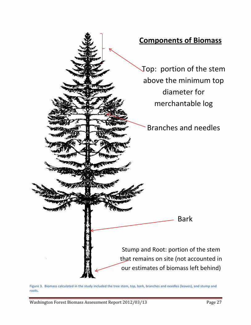
Figure 3 describes the various components of the tree that we considered in our calculations of biomass. There exist several alternative sets of equations that relate tree metrics such as diameter at breast height (DBH) to the various components of the tree. Equations that estimate the volume of stem biomass in dry weight units are presented in Appendix 4. For each tree harvested, we compiled the component biomass and recorded its weight in a tabular format. The biomass table was stored in a database and linked to another database that described the ownership and location of the harvested trees.
Washington Forest Biomass Assessment Report 2012/03/13 Page 27
Figure 3. Biomass calculated in the study included the tree stem, top, bark, branches and needles (leaves), and stump and roots.
Components of Biomass
Top: portion of the stem above the minimum top
diameter for merchantable log
Branches and needles
Stump and Root: portion of the stem that remains on site (not accounted in our estimates of biomass left behind)
Bark

Washington Forest Biomass Assessment Report 2012/03/13 Page 28
Figure 4. Alternative computational methods considered for the study to determine the volume of biomass in the stem for Douglas fir stem biomass.
Several alternative equations for biomass calculations exist in the literature. We conducted a comparative analysis for a variety of biomass computational approaches. The biomass calculations were implemented in Visual Basic Application language using spreadsheets to provide flexibility in computation and avoid errors in copying formulas. The calculations were done for a variety of species across a range of diameters. Figure 4 illustrates the stem portion of the tree biomass using 5 different equations. Equations for other components of residual biomass were similarly studied. In Figure 4 Gholz refers to our implementation of Gholz allometric equations for biomass estimates by component. Jenkins refers to implementation of Jenkins allometric equations for biomass estimation by component. CORRIM1 is based on the Jenkins equation. It uses wood specific gravity calculations for volume entered from the growth model and compares it to Jenkins’ stem biomass, and then scales the component biomass. CORRIM2 is based on Jenkins component proportions. It implements independent volume (smalian's) calculation for cubic volume, and then scales the component biomass. Browne is taken from Browne (1962) and uses a mature and young age classification to consider different biomass functions for trees of different diameters. After comparing the various computational methods, the study chose the Browne approach since it had been used previously to model biomass in Washington by members of the study team and was in the middle of the group of the models examined (Appendix 4).
0
2
4
6
8
10
12
1 5 10 15 20 25 30 35 40 45
Biom
ass i
n po
unds
(100
0's)
DBH in inches
Gholz Jenkins CORRIM1 CORRIM2 Browne

Washington Forest Biomass Assessment Report 2012/03/13 Page 29
2.2.2. Outlining the Process of Biomass Calculations The calculations began by describing typical forest operations currently being practiced across Washington state and then developing a harvest scenario matrix. Next, a management prescription was implemented, and the biomass volume as a byproduct of a forest operation determined, following Browne’s biomass equations. This volume of biomass was subjected to harvest configuration constraints to generate the volume reaching the roadside. The roadside volume was subjected to operability constraints, such as road limitations, to determine the potential market biomass. The potential market biomass was filtered through economic constraints, such as the cost to process and haul material to mills, to determine the volume of biomass that was delivered to a facility. The report begins to describe this process below starting with the forest operations that were studied.
2.2.3. Developing the Harvest Scenario Matrix The study team produced a scenario matrix that established the harvest activities utilized by logging operators, and included forest operations on pre-commercial thinning activities as requested by the scope of work. We used this matrix to develop the management scenarios used with the FVS models described previously.
Table 2. Summary of harvest and forest operation scenarios
Harvest and Forest Operation Scenarios Harvest and Forest Operation Scenarios RH remnant stands >50 years RH remnant stands >65 years No PCT, RH @ 35 years No PCT, RH @ 45 years No PCT, RH @ 50 years No PCT, RH @ 55 years No PCT, RH @ 60 years No PCT, RH @ 65 years No PCT, RH @ 70 years No PCT, RH @ 75 years No PCT, RH @ 80 years RH @ 90 years No PCT, CT @ 25 years, RH @ 45 years No PCT, CT @ 30 years, RH @ 50 years No PCT, CT @ 35 years, RH @ 65 years No PCT, CT @ 40 years, RH @ 65 years No PCT, CT @ 45 years, RH @ 65 years No PCT, CT @ 55 years, RH @ 85 years CT or PC @ 55 years
PCT @ 6 years, RH @ 35 years PCT @ 12 years, RH @ 45 years PCT @ 15 years, RH @ 45 years PCT @ 15 years, RH @ 50 years PCT @ 15 years, RH @ 60 years PCT @ 15 years, RH @ 75 years PCT @ 17 years, RH @ 55 years PCT @ 15 years, CT @ 45 years, RH @ 65 years PCT @ 15 years, CT @ 55 years, RH @ 85 years PCT @ 20 years, PT @ 70 years - thinning from above and below PC - from above and below PC - thinning from above and below PC - thinning from above & below w/RH @ 55 yrs PC - thinning from above & below w/RH @ 60 yrs PC - thinning from above & below w/RH @ 65 yrs PC - thinning from above & below w/RH @ 75 yrs PC @ 65 years - thinning from above and below PC @ 70 years - thinning from above and below PC @ 75 years - thinning from above and below
Source: Study survey data (RH, regeneration harvest; PCT, precommercial thinning; CT, commercial thinning; PC, partial cut)
Table 2 summarizes the harvest scenarios developed by the study team. The large number of alternatives was developed as requested by the contract to include various thinning options. While

Washington Forest Biomass Assessment Report 2012/03/13 Page 30
there are many alternatives listed, they are not all necessarily associated with commercial timber harvest. As is described later in the report, the study team chose those management treatments currently practiced in Washington based on survey results for various landowners.
To develop the scenarios, the study team first reviewed the management alternatives that were considered for the recently completed Washington Timber Supply Study (WTSS, 2006). A discussion of the management alternatives was held internally and recommendations for changes of the WTSS management alternatives were made. The recommendations were to canvas landowners through telephone calls, email and site visits to determine their management and/or silvicultural prescriptions by forest ecosystem type. A preliminary table containing forest ecosystem, owner class, region, harvest scenario, estimated percent of activity and comments was developed from the initial information gathered. We continued to canvass the owners not included in the preliminary table to improve our understanding of management practices across owner groups. The harvest scenario matrix is presented in Appendix 5. It describes the forest operation by owner class and forest ecosystem type. For some owners the study team obtained their best estimate breakout of their activity implemented on their lands. We extracted all scenarios from Appendix 5 and listed them in Table 2.
Many of silvicultural regimes listed in Table 2 were simulated using the appropriate FVS models to represent a wide variety of actual and potential forest management regimes practiced within different ownership classes, management zones, and forest types. Regimes were developed from three types of treatments: a precommercial thin (PCT), commercial thin (CT), and/or regeneration or final harvest (RH). Within the 30 year planning period, a regime could include no treatments (no action), PCT only, CT only, RH only, PCT and CT, CT and RH, and RH and PCT. The full set of possible simulations was then developed by varying the timing and intensities of the treatments. Approximately 3,000 unique regimes were developed and applied to each segment of the landscape. The final number of regimes simulated depended on FCID forest type, age, and management zone. In total, over 5 million simulations were run using programs written in Python script. These simulations produced a database of harvest activity alternatives from which we selected those commonly practiced today. For example, a heavy commercial thinning activity that reduced basal area to 45 square feet was chosen to study forest health treatment effects in eastern Washington on market biomass production. An alternative activity chosen was one that used a lighter thinning response, such as removing all trees smaller than 12” diameter breast height (DBH).
Precommercial Thin Precommercial thins were simulated at age 15 on the Westside and age 20 on the Eastside. All precommercial thins retained the largest 300 trees per acre (TPA) by DBH.
Commercial Thin Commercial thins were simulated at all ages greater than a minimum age. The minimum age was 30 on the Westside and 50 on the Eastside. For example, for a 30 year old stand on the Westside, 5 CT only simulations were developed: CT in 2010, CT in 2015, CT in 2020, CT in 2025, and CT in 2030. All thinnings were implemented from below by diameter limit.

Washington Forest Biomass Assessment Report 2012/03/13 Page 31
Two intensities of CT’s were simulated. On the Westside, a light CT retained the largest 250 TPA, while a heavy CT retained the largest 150 TPA. One the Eastside, one CT simulation removed all trees smaller than 12” DBH (standard forest health treatment), while another harvested down to 45 square feet of residual basal area. In most stands, removing all trees below 12” DBH was a lighter thinning.
Final Harvest Like CT, final harvests were simulated at all ages greater than a minimum age. The minimum age depended on the half-state, forest type and ownership class. For CT and RH regimes, RH was scheduled at least 30 years after CT on the Westside.
Final harvest intensities varied by forest type, ownership class and management zone. All treatments were simulated as cutting from below by diameter limit. Treatments were modeled to meet existing Washington state forest practices regulations. For example, uplands were harvested to 5 TPA in all cases. Inner riparian buffers were harvested to 100 TPA on the Eastside and 58 TPA on the Westside. Outer riparian buffers were harvested to 10 TPA in all Westside cases and Ponderosa pine forests on the Eastside. All other Eastside outer buffers were harvested to 20 TPA. Wetland buffers were harvested to 75 TPA in all cases.
2.2.4. Calculating Post-Timber Harvest Biomass The first step to calculate the post-timber harvest biomass volume was to define a target level of harvest for a given area. The target level was used to constrain harvest activity up to the targeted volume in a specific area and for a specific ownership. Harvest targets were defined by county and ownership based on published WADNR harvest reports (WADNR, various years). The use of small geographical area such as a county by ownership, rather than a statewide target for example, to establish the target level had the benefit of identifying when ownerships in counties were not able to meet the targeted harvest requirement. This information was recorded in the database to allow the user to identify limiting local supply constraints. The target harvest level was developed by considering past harvest levels.
A sensitivity analysis of harvest levels was conducted using three alternate harvest target outlooks producing a conservative, mid-range and aggressive harvest projection by county and ownership. The three harvest outlooks were developed to encase the recent historic levels observed in the WADNR harvest reports.
As mentioned above, the study utilized the DNR Harvest Reports from 2000 to 2009 (latest available) to develop the forest operations required to update the inventory to 2010 conditions. Since tribal harvests are not included in the DNR Harvest Reports, a harvest rate was inferred for the tribal management class for the period 2000 to 2009 (see Table 3 and Table 4).

Washington Forest Biomass Assessment Report 2012/03/13 Page 32
Table 3. Eastside Harvest Levels
1980 1985 1990 1995 2000 2005 2009
Native American
277,827 148,384 144,712 194,217 294,790 150,000 150,000
Forest Industry
228,251 380,248 406,466 262,170 214,039 100,036 19,986
Private Large
85,308 26,838 56,230 66,356 91,958 76,482 79,031
Private Small
95,240 127,920 152,497 285,050 202,522 239,721 30,576
State 205,133 93,545 84,245 82,667 87,640 97,737 80,591 Other Non-federal
13,560 227 13,940 13,670 1,178 57,266 29,276
National Forest
258,217 324,138 313,259 71,306 59,743 52,455 63,565
Other Federal
1,884 2,744 4,443 0 923 3,906 22
Total 1,165,420 1,104,044 1,175,792 975,436 952,793 777,603 453,047 Source: WADNR Harvest Reports various years
Table 4. Westside Harvest Levels
1980 1985 1990 1995 2000 2005 2009
Native American
58,401 64,869 37,614 35,805 35,394 35,000 35,000
Forest Industry
2,707,342 2,211,656 2,143,755 1,752,936 1,610,234 858,022 518,197
Private Large
159,146 430,450 830,195 435,939 580,313 913,992 541,229
Private Small
232,146 384,296 557,685 687,517 477,728 618,431 204,796
State 702,160 919,780 573,129 413,531 471,614 496,144 560,858 Other Non-federal
16,810 26,768 15,983 6,180 15,321 0 0
National Forest
771,896 803,518 503,952 78,904 21,605 28,687 51,873
Other Federal
13,076 18,162 11,122 6,275 11,566 27,702 37,311
Total 4,660,977 4,859,499 4,673,435 3,417,087 3,223,775 2,977,978 1,949,264 Source: WADNR Harvest Reports (various years)

Washington Forest Biomass Assessment Report 2012/03/13 Page 33
The harvest target was met assuming one of the silvicultural regimes listed in Table 2. With the harvest level target in hand, we queried the inventory database to select parcels that contained harvestable volumes of timber by county and ownership until our harvest target was met. We then recorded the volume of biomass by components associated with trees harvested. A defect measure was added to account for defects of the tree stem. Interviews with operators suggested a range of 3% to 25% was commonly used, depending on ownerships, species, and stand conditions. We included a 10% breakage and defect measure to account for the portion of stem volume that was defective as commercial volume (log sweep, decay) and breakage as trees are felled.
The timber resource and subsequent harvest characteristics within the state of Washington has been migrating from one of large timber to harvest of younger, smaller stands. In addition, the increased utilization of mechanized logging sites has reduced overall breakage and defect from harvested stands. Landowners and managers of public agency lands indicated the breakage and defect ranged between 3% and 5% for the majority of the volume harvested. However, there is always a portion of the resource consisting of older stands or stand of higher than average defect. These constitute a small minority of the total volume harvested in any given year. Breakage and defect was estimated to be 10% overall to represent a conservative volume that would include atypical stands of significantly higher than average defect and adequately represent the majority of the volume harvested within Washington.
The method employed by the study to distinguish the portion of the post-timber harvest biomass volume that is moved to a roadside or landing is described next.
2.2.5. Determining Harvest Configuration Constraints Post-timber harvest biomass was divided into biomass that was piled or brought to a roadside (harvested biomass) or remained scattered on site (residual harvested biomass). The amount of biomass reaching a landing or roadside was dependent on the harvest configuration used by logging contractors. Using our surveys, we solicited information regarding harvest system configuration from landowners or land managers that utilized various equipment configurations to determine the volume of post-timber harvest biomass that reached a landing or roadside. The information on harvest configuration collected included:
• Ground-based yarding, manual felling, manual or mechanical processing, log yarding, tops left in unit;
• Ground-based yarding, mechanical cut-to-length (CTL), tops left in unit; • Ground-based yarding, manual felling, manual or mechanical processing, whole tree or log
yarding including tops; • Ground-based yarding, mechanical CTL, logs including tops yarded; • Ground-based yarding, mechanical felling, whole tree yarding; • Cable yarding system, manual felling, manual processing, log yarding, tops left in unit; • Cable yarding system, manual felling, manual or mechanical processing, whole tree or log
yarding including tops.

Washington Forest Biomass Assessment Report 2012/03/13 Page 34
These estimates were summarized by owner to develop four basic harvest system configuration categories:
• Ground-based yarding without whole tree or logs and tops yarded; • Ground-based yarding with whole tree or logs and tops yarded; • Cable yarding system without whole tree or logs and tops yarded; • Cable yarding system with whole tree or logs and tops yarded.
The harvest system configuration was reported as the percentage of forest operations employing either cable or ground-based yarding systems and requiring yarding of whole trees or tops as opposed to NO whole trees or top yarding requirement. A summary of field and phone interviews was developed to separate cable and ground-based yarding operations that did not include whole tree or top yarding. Since forest operations that do not include whole tree or top yarding were not considered suitable candidates for biomass recovery, we assumed their associated recoverable wood fiber remained scattered throughout the operation unit as opposed to accumulating roadside or in central landing locations. The following series of 6 panels in Figure 5 describes the percentage of forest operations under the alternative harvest system configurations by Washington Department of Revenue Stumpage Valuation Area (SVA) (see figure 18).
SVA1
0%10%20%30%40%50%60%70%80%90%
100%
GB, WT or Tops GB, No WT or Tops
Cable, WT or Tops Cable, No WT or Tops

Washington Forest Biomass Assessment Report 2012/03/13 Page 35
SVA2
SVA 3
0%10%20%30%40%50%60%70%80%90%
100%
GB, WT or Tops GB, No WT or Tops
Cable, WT or Tops Cable, No WT or Tops
0%10%20%30%40%50%60%70%80%90%
100%
GB, WT or Tops GB, No WT or Tops
Cable, WT or Tops Cable, No WT or Tops

Washington Forest Biomass Assessment Report 2012/03/13 Page 36
SVA 4
SVA 5
0%10%20%30%40%50%60%70%80%90%
100%
GB, WT or Tops GB, No WT or Tops
Cable, WT or Tops Cable, No WT or Tops
0%10%20%30%40%50%60%70%80%90%
100%
GB, WT or Tops GB, No WT or Tops
Cable, WT or Tops Cable, No WT or Tops

Washington Forest Biomass Assessment Report 2012/03/13 Page 37
Eastside (SVAs 6, 7 and 10) Figure 5. Harvest system distribution weighted by volume for ownership and forest type (Source: study survey data)
The percentage of each of the four basic harvest system configuration categories was weighted by owner or land management type using estimated annual harvest volume by forest ecosystem within each SVA for operations on the westside of the state. Operations on the eastside of the state from SVA 6, 7 and 10 were combined into a single data set. The choice to use SVA as the spatial aggregated regions was made to maintain confidentiality for those ownerships easily identifiable by county. Additionally, SVA presented a convenient regional definition already used widely to measure timber valuation across similar regions. Ownerships were aggregated into classes including private ownerships (industrial, non-industrial and municipally owned), tribal, the Washington Department of Natural Resources, the Washington Department of Fish and Wildlife, and federally managed lands. The study team used the weighted percentage of each harvest system by owner class by forest ecosystem by SVA or for the entire eastside of Washington to determine the volume of post-harvest biomass that reached a landing or roadside.
Figure 5 shows the harvest system distribution weighted by volume for each SVA, ownership and forest type. Brown-colored areas in bars reflect no whole tree or tops yarded implying branches and tops remained scattered throughout the unit. Green-colored areas reflect whole tree and tops yarded creating additional volume in piles and alongside roads.
2.2.6. Calculating Harvested Biomass Given the volume of biomass generated in tops, branches and foliage from our previous stage, we used the weighted percentage of the harvest configuration associated with each SVA, ownership and forest type and slope to determine the volume of biomass in tops, branches and foliage that reached the landing or roadside. Slope was used as a proxy to equipment limitation. A breakpoint of 30% was used
0%10%20%30%40%50%60%70%80%90%
100%
GB, WT or Tops GB, No WT or Tops
Cable, WT or Tops Cable, No WT or Tops

Washington Forest Biomass Assessment Report 2012/03/13 Page 38
to distinguish between cable and ground yarding operations. So far, for each parcel, we know the amount of harvest volume, and the associated biomass by components of the trees harvested. This section added the study’s assumptions about harvest configuration gained from survey information to determine two biomass volumes: harvested biomass, and residual harvested biomass. The latter refers to the volume of biomass in tops, branches and foliage, as well as stem volume defect that remain scattered throughout the site due to our assumptions on harvest equipment configuration and their ability or desire to conduct whole tree or top yarding. It was the volume that breaks off or was cut in the woods and left scattered as commercial logs were brought to the landing. The calculated harvested biomass volume was carried forward in our calculus of potential market biomass (Figure 6).
Figure 6. Post-timber harvest biomass conversion into harvest biomass pathway
2.2.7. Determining Potential Market Biomass Operability Constraints Biomass on a parcel began as post-timber harvest biomass. It was everything that was generated as the byproduct of a forest operation, including tops, live and dead branches, foliage and defect. The part of the post-timber harvest biomass that was brought to the landing and roadside was noted as harvested biomass and described in the previous section. This calculated harvested biomass volume was then filtered by operability constraints for each SVA, ownership and forest type, and became either potential market biomass or residual potential market biomass. The potential market biomass represents the amount that could be potentially loaded on the truck. The residual potential market biomass was the portion that did not get loaded due to operability constraints, e.g., equipment could not be brought in, or other factors such as landowner preferences, e.g., the landowner did not want to sell their biomass. The portion of harvested biomass that was not operable became residual and remained on site.
Operability implied that the ownership had appropriate infrastructure, including road system, landing size and location to accommodate effective biomass processing and removal. The study team summarized survey information and calculated the percentage of the ownership suitable for biomass
Post-timber Harvest Biomass
Harvest Configuration
Harvested Biomass
Residual Harvested Biomass

Washington Forest Biomass Assessment Report 2012/03/13 Page 39
recovery based on their responses regarding the appropriate infrastructure that existed for biomass removal. In addition, the operability percentage reflected current operating capabilities of local and/or regional biomass processing companies. We used the operability percentage to identify the portion of the ownership conducive to biomass recovery.
To develop the operability percentage, landowners or land managers were requested to provide an estimate of the ownership with infrastructure suitable, e.g., roads and landings, for effective biomass recovery based upon their knowledge and familiarity with the operating capabilities and limitations of local and/or regional biomass processing companies. In addition local and regional biomass processing companies with experience on the subject and land owners/managers were contacted to solicit their estimate of operability with regard to their ability to process biomass effectively relative to ownership infrastructure and current market conditions. If there was substantive difference, i.e., greater than 10%, between the estimates provided by the landowner and biomass processor, the midpoint was employed to represent the operability filter percentage.
The percentage was subsequently weighted by harvest volume by forest ecosystem by ownership within the individual SVA for westside ownerships. The eastside was included as a single area for this evaluation (SVA 6, 7, and 10). The ownerships were aggregated into private owners, tribal, Washington Department of Natural Resources, Washington Department of Fish and Wildlife, and federally-managed lands. Each ownership class within each SVA for the westside of the state, for each forest ecosystem had a distinct operability percentage reflecting infrastructure, markets, and local and/or regional biomass processor capabilities and limitations (Figure 7, presented as a series of 6 graphs by SVA region).
SVA 1
0%10%20%30%40%50%60%70%80%90%
100%
Federal Private Tribal WA DFW WA DNR
DF
RA
TF/MC
WH

Washington Forest Biomass Assessment Report 2012/03/13 Page 40
SVA 2
SVA 3
SVA 4
0%10%20%30%40%50%60%70%80%90%
100%
Federal Private Tribal WA DFW WA DNR
DF
RA
TF/MC
WH
0%10%20%30%40%50%60%70%80%90%
100%
Federal Private Tribal WA DFW WA DNR
DF
RA
TF/MC
WH
0%10%20%30%40%50%60%70%80%90%
100%
Federal Private Tribal WA DFW WA DNR
DF
RA
TF/MC
WH

Washington Forest Biomass Assessment Report 2012/03/13 Page 41
SVA 5
Eastside SVAs 6, 7 and 10 Figure 7. Recovery percent based upon operability conditions DF = Douglas fir type, RA = hardwood type, PP = Ponderosa pine type, TF/MC = True fir, mixed conifer type, WH = western hemlock type. (Source: Study survey data).
2.2.8. Calculating Potential Market Biomass The calculus of biomass has progressed to the point where the study team determined the volume of biomass at the roadside or landing that has the potential to get loaded onto a truck. It was the volume of harvested biomass multiplied by the operability percentage and was referred to as the potential market biomass. As in the case of the harvested biomass, there was a portion of the potential market biomass that became residual potential market biomass since it could not be loaded onto a truck because the equipment could not get to it or similar factors as previously described (Figure 8).
0%10%20%30%40%50%60%70%80%90%
100%
Federal Private Tribal WA DFW WA DNR
DF
RA
TF/MC
WH
0%
10%
20%
30%
40%
50%
60%
70%
Federal Private Tribal WA DFW WA DNR
DF/WF
PP
TF/MC
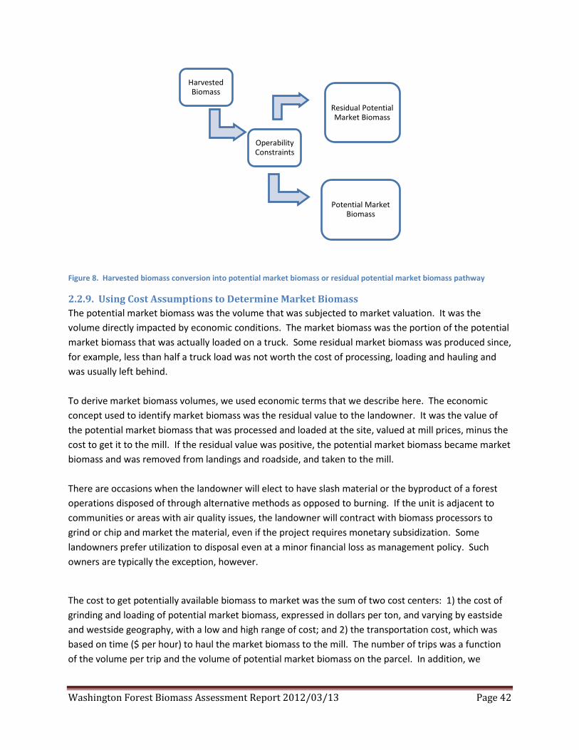
Washington Forest Biomass Assessment Report 2012/03/13 Page 42
Figure 8. Harvested biomass conversion into potential market biomass or residual potential market biomass pathway
2.2.9. Using Cost Assumptions to Determine Market Biomass The potential market biomass was the volume that was subjected to market valuation. It was the volume directly impacted by economic conditions. The market biomass was the portion of the potential market biomass that was actually loaded on a truck. Some residual market biomass was produced since, for example, less than half a truck load was not worth the cost of processing, loading and hauling and was usually left behind. To derive market biomass volumes, we used economic terms that we describe here. The economic concept used to identify market biomass was the residual value to the landowner. It was the value of the potential market biomass that was processed and loaded at the site, valued at mill prices, minus the cost to get it to the mill. If the residual value was positive, the potential market biomass became market biomass and was removed from landings and roadside, and taken to the mill. There are occasions when the landowner will elect to have slash material or the byproduct of a forest operations disposed of through alternative methods as opposed to burning. If the unit is adjacent to communities or areas with air quality issues, the landowner will contract with biomass processors to grind or chip and market the material, even if the project requires monetary subsidization. Some landowners prefer utilization to disposal even at a minor financial loss as management policy. Such owners are typically the exception, however.
The cost to get potentially available biomass to market was the sum of two cost centers: 1) the cost of grinding and loading of potential market biomass, expressed in dollars per ton, and varying by eastside and westside geography, with a low and high range of cost; and 2) the transportation cost, which was based on time ($ per hour) to haul the market biomass to the mill. The number of trips was a function of the volume per trip and the volume of potential market biomass on the parcel. In addition, we
Harvested Biomass
Operability Constraints
Potential Market Biomass
Residual Potential Market Biomass

Washington Forest Biomass Assessment Report 2012/03/13 Page 43
introduced an equipment setup cost that constrained the marketability of biomass by a minimum volume required to cover the cost associated with moving processing and haul equipment to the site.
2.2.10. Cost Center Definitions The study team first calculated the minimum volume economically feasible per truck load. This calculation was made using information on average haul rate ($ per hr.), the haul time (hr.), load time (hr.), the load rate ($ per BDT) and a market price ($ per BDT). Second, the study determined the return to the landowner based on a profit function that considered a move-in cost, the volume of potential market biomass, the minimum economic tons per truck load and market price.
On-site Cost Center The production costs associated with biomass processing and delivery were developed through consultation with various biomass processing contractors throughout Washington state. In general, the existing infrastructure associated with biomass production exists primarily in close proximity to current markets. In Washington state, the primary markets for biomass material for conversion to heat/steam and power are concentrated in the forest products manufacturing sector, primarily the pulp and paper industry, with some material also purchased by newer forest product mills augmenting mill residue with forest-based biomass materials.
The typical equipment employed in the production of biomass material could include a grinder (either rubber-tired or track mounted), one or two excavators for collecting, aggregating or loading slash, and chip vans. Additional equipment might include a front-end loader for moving processed biomass material into chip vans; a dozer for road modification, landing improvement or pushing slash piles; a skidder for pushing slash, moving the grinder or hauling the chip truck and van up adverse grades; road grader; a low bed trailer for moving equipment; and off-road dump trucks for relocating processed or unprocessed material to a central location of suitable size. The range of estimated hourly rates to operate such equipment is shown in Table 5 below.
Table 5. Equipment cost per hour
EQUIPMENT LOW RANGE
HIGH RANGE
Skidder $75 $95 Excavator $125 $150 Grinder $300 $400 Road Grader $75 $100 Water Truck $65 $85 Low Bed (conventional) $110 $120 Low Bed (heavy loads) $125 $140 D5 or D6 CAT Dozer $75 $95 Source: Study survey data
The production costs associated with processing slash into biomass suitable for boiler fuel and loading into chip vans was influenced by a number of factors, including road configuration (surface, grade,
Washington Forest Biomass Assessment Report 2012/03/13 Page 44
corners, available places to turn chip van around), pile volume, proximity of other landing piles within harvest or treatment unit, number of units (if multiple small harvest or treatment units are included within sale), sawlog or pulp log merchandizing specifications, to name but a few.
The range of production costs for processing and loading (into vans for transport to end user) biomass material sourced from sustainable forest operations was from $16 to $35 per BDT for operations on either east or west side of the state of Washington. The range of costs when weighted by estimated volume production by biomass processing contractor was from $22 to $28 per BDT for eastside operations and from $25 to $29 for westside operations.
The array of production costs represented the various business models and equipment configurations employed in the process. A contractor may confine the operation for accessing only slash piles of specified minimum volume and proximity to minimize equipment requirements to a grinder and excavator for loading directly into chip vans for transport. Such an operation will generally operate at lower production costs. Another contractor may be required to aggregate material into suitable piles along roadsides for loading into the grinder. This could require an additional excavator on site. If the road system did not accommodate chip van access to the grinder operation, the contractor might load processed material into off-road dump trucks. This processed biomass was then delivered to a central location accessible to chip vans and unloaded onto the ground. When a chip van arrived, a front-end loader was used to move processed biomass material from the pile into the van for delivery to market.
Transportation Cost Center The cost of transport varied with van capacity, travel speed (navigating forest roads requires slower travel speed), distance to market, as well as time required to load and unload. Biomass processing contractors employed an array of chip van sizes. Depending upon circumstances, a contractor may utilize two smaller chip vans in tandem. Such configuration may be necessary to access the operation, even though additional time would be required for loading, hooking up both trailers, and unloading each. Some contractors restricted their operations to utilizing only 53 foot chip vans (more efficient, but operate best on pavement); either modifying roads to accommodate access or declining operations where such chip vans were not suited. The range of hourly rates for transporting processed biomass material as provided by trucking companies and biomass processing contractors was from $70 to as much as $115 per hour. The average was estimated at $85 per hour.
The assumptions employed for travel speed were 20 mile per hour over forest roads, posted speed limits for rural roads, and 45 mile per hour over highways. There are exceptions for substantive travel using interstate highways where average travel speed would be 55 miles per hour (such as the Interstate 5 corridor).
2.2.11. Calculating the Residual Value to the Landowner Survey information was used to calibrate a net revenue function that considered a move-in cost, the volume of potential market biomass, the minimum economic tons per truck load and market price. The minimum economic tons per truck were a function of the market price, time to load and haul and their respective rates. We expressed this relationship as:

Washington Forest Biomass Assessment Report 2012/03/13 Page 45
Market Price = (Haul Rate*Haul Time + Haul Rate*Load Time)/Volume (Bone Dry Ton (BDT)) + Load Rate
The Haul Rate is transportation cost ($76 to $114 per hour) The Load Rate is the average equipment costs ($21 to $31 per BDT) Market Price, Haul Time and Load Time are allowed to vary to produce the minimum economic load per truck at the given Haul Rate and Load Rate for the specific haul time specified. Haul and load rates can be changed to produce new minimum economic loads per truck. Adding the movement of equipment costs completed the profit function specification to determine the residual value to the landowner.
Figure 9. Price and tonnage of market biomass relationship (First number is the haul rate; second number is the processing cost; third number is the move-in costs. 160/20@100 uses $160 haul rate, $20 processing rate and $100 move-in cost)
The economic model established the break-even residual value for the landowner. Figure 9 depicts this value at different haul and load rates at two move-in cost levels for a given market price and potential market price availability. The break-even residual value point was used to decide whether potential market biomass was loaded onto a truck or not. A point indicating a volume of potential market biomass at its market price to the right of each curve indicates a positive residual value; a point to the left of the curve indicates a negative residual value to the landowner. Only points associated with
-
200
400
600
800
1,000
1,200
$30.00 $35.00 $40.00 $45.00 $50.00 $55.00 $60.00 $65.00 $70.00
BDT
Pote
ntia
l Mar
ket B
iom
ass
Avai
labl
e
Market Price ($/BDT)
160/20@100
85/35@100
100/35@100
100/20@100
85/26@100
85/26@200

Washington Forest Biomass Assessment Report 2012/03/13 Page 46
market prices to the right of each curve are considered marketable biomass. Points to the left of each curve resulted in potential market biomass that is assumed to be left behind, i.e., the biomass volume became residual potential market biomass.
Figure 9 also represents a sensitivity analysis on alternative values of move-in costs, haul rates and processing costs. Each curve indicates a different value of haul cost, load rate and movement of equipment cost. The load and haul time were assumed to be one hour each. The labels in the chart legend indicate each of these cost assumptions. For example, the curve labeled “160/20@100” refers to a haul cost of $160 per hour, a load rate of $20 per ton at a move-in cost of $100. The position of this curve is not much different than curve “80/35@100”. The higher load rate, i.e., equipment cost, is offset by almost halving the haul rate, i.e., transportation cost. Reducing the load rate from $35 to $26 (“85/35@100” to “85/26@100”), while maintaining the haul rate and move-in cost constant, shifts the curve leftward, reducing the market price at which residual values are at a break-even point by the same amount, i.e., $9. Increasing the haul rate from $85 to $100 per hour shifts the break-even residual value curve to the right, increasing the needed market price by about $6 per BDT for biomass to become marketable. Finally doubling the move-in cost of equipment shifted the break-even curve to the right and changed the shape of the curve, increasing the market price by varying amounts depending on the volume of potential market biomass at the site. As potential biomass volume declined the price rise necessary to offset the higher movement of equipment costs increased.
2.2.12. Conducting Network Analysis A network analysis was undertaken to calculate travel times in minutes and distances in miles from every parcel to every facility. The facility is either the location of an existing facility or a hypothetical facility that was solicited by the interested public during the project’s second public meeting. This produced concentric 10 minute time rings and five mile distance rings around each facility. Time from each facility was calculated to four hours and distance was calculated to 200 miles. Figure 10 is an example of the areas within a one-hour drive time surrounding a facility. The green area comprises concentric circles each ten minutes apart.

Washington Forest Biomass Assessment Report 2012/03/13 Page 47
Figure 10. Example concentric service area rings around a facility for a one-hour drive time.
2.2.13. Calculating Market Biomass Potential market biomass in each concentric ring was assigned a residual value. Then the cost value was compared to the residual value at a given market price to determine whether the biomass within the concentric circle was marketable or not (Figure 10). The results produced by analyzing the production cost to processors and haulers on potential market biomass were:
1. Residual values (anything positive is within the supply shed for the mill in question) for each parcel for the landowner, and
2. Volume of market biomass removed from the site (i.e. number of trips made by volume hauled).
These values were recorded in the database (http://wabiomass.cfr.washington.edu/). In summary, the volume of market biomass was determined using the residual value calculations described above and defining market biomass as the volume of potential market biomass that has a positive residual value based on network analysis. The market biomass was the volume of biomass that makes it to the facility.

Washington Forest Biomass Assessment Report 2012/03/13 Page 48
Changes in the study assumptions likely will have an influence in the volume and value of potential market biomass. Factors that might change the market biomass volume were a change in the harvest configuration that brings slash to the roadside or landing, e.g., creating a larger volume of potential market biomass, a change in the operability, e.g., creating a greater portion of potential market biomass that was potentially loaded, and cost/price changes, or any combination of these three. Further analysis of future potential gains in efficiencies associated with harvest configuration, operability or cost structure is recommended.
Figure 11. Potential market biomass conversion into market biomass pathway
2.2.14. Calculating the Volume of Biomass Left Behind To calculate the volume of biomass remaining at roadside and in piles, as well as scattered throughout the site, the study summed the residual harvested volume, the residual potential market biomass and residual market biomass from the previous three sections (see Figures 6, 8 and 11). In addition, the range of pre-existing downed-woody material was added to the residual harvest volume. Figure 12 presents a complete picture of the flow of biomass volume starting with a forest operation through market biomass, adding to it the component of preexisting woody material. The volume of biomass left behind comprised the residual volumes as a result of a forest operation plus the estimated volume of pre-existing woody material. The range of pre-existing woody material was provided by consulting the decayed wood advisor (DecAID, US Forest Service). The residual values are highlighted with bold font in the figure. Pre-existing downed woody material was derived from DecAID, a decision making tool produced by the USDA Forest Service (Marcot, et al. 2010). DecAID presents information on snag diameter, snag density,
Potential Martket Biomass
Cost Considerations and Market Price (Residual Value)
Market Biomass
Residual Market Biomass

Washington Forest Biomass Assessment Report 2012/03/13 Page 49
down wood diameter, and down wood percent cover, and on the range of natural (unharvested) and current (all) conditions of snag density and down wood percent cover by diameter classes. The information is presented at three statistical tolerance levels which may be interpreted as three levels of “assurance:” where a 30% tolerance level indicates 30% of the wildlife population would be found in conditions with up to this amount of downed wood and snags, a 50% tolerance level at which 50% of the population could be found utilizing areas with this amount of wood, and a 80% tolerance level where 80% of the population could be found in forests with this amount of wood or less. Our study mapped wildlife habitat types using county, FVS variant and forest types to cross-map the statistical tolerance levels, and report the 80% tolerance level to find the range in which 80% of the plots would be found. The range reported was 0 BDT per acre, since there were plots that did not have any down wood diameter, to 7.2 million BDT per acre.
Figure 12. The volume of biomass that was left behind (indicated by boldface type) defined by three sources of residual biomass left on site as a result of a forest operation plus pre-existing woody material.
Post-timber Harvest Biomass
F
ores
t Ope
ratio
n
Pre-existing woody material
Merchantable Stem Volume
Harvested Biomass
Potential Market Biomass
Market Biomass
Residual Harvested Biomass
Residual Potential Market Biomass
Residual Market Biomass

Washington Forest Biomass Assessment Report 2012/03/13 Page 50
2.3. Biomass Database Design
2.3.1. The Washington State Biomass Database The previous sections described the process to develop the volume of market biomass and its residual value to the landowner. These data were complimented by parcel data to form the Washington State Biomass database (http://wabiomass.cfr.washington.edu/. Other data were also used to complete the biomass database and all are described below.
The parcel database (Rogers and Cooke 2006) was updated with 2009 parcel data for this study. New data was acquired that included roads, stream buffers, streams, lakes and wetlands, ownership, slope and elevation. The biomass database also has a satellite imagery layer. Links were created between the parcel database and the statewide inventory and harvest activity data to form the Washington State Biomass Database. This database provided information on the location of harvest activities and their resultant biomass production, and the study used it to calculate residual value to the landowner, and subsequently the amount of market biomass volume produced.
The Washington State Biomass Database integrated many input layers together into a seamless statewide mosaic of landscape segments. On average the 37 million geographic segments were less than 1 acre in size and represented a unique combination of owner, forest inventory, slope class, and management zone (core, inner, outer and wetland buffers, uplands, reserves, special management areas) (Figure 13). Each geographic segment had a unique inventory created from the FCID plot from the LEMMA work described earlier and its associated FVS modeling work that was specific to that place on the landscape. The forest was treated accordingly to the various combinations of owner, inventory, slope class, and management zone based on the management alternatives and silvicultural options already described. To allow for harvest and forest operation option analysis, each geographic segment was associated with all the possible harvest and forest operation options that conformed to the specific management class and zone.

Washington Forest Biomass Assessment Report 2012/03/13 Page 51
Figure 13. Combined "segments" in the database
For example, in Figure 13, various segments are depicted in the upper left snapshot. The forest land use layer is provided in the snapshot in the upper right corner. The management class layer from parcel information was overlaid in the middle left snapshot. Information on riparian zones was overlaid in the middle right snapshot. Slope class, used to assign harvest configuration alternatives, is demonstrated in the lower left picture. Inventory from plot information and the modeling exercise is shown in the lower left frame. Each segment was treated and the resulting post-harvest biomass was calculated to develop the supply of market biomass over time, as well as the volume left behind as a byproduct of a forest operation.

Washington Forest Biomass Assessment Report 2012/03/13 Page 52
2.3.2. The Harvest Scenarios Our first step in creating a harvest scenario run for the assessment of market biomass was to calibrate all plots to a common year. Then we implemented a range of silvicultural treatments taken from Table 2 to produce the harvest activity, which were used to produce the post-timber harvest biomass volumes and subsequent volumes of marketed biomass.
The east and west side GNN inventory had nominal dates of 2000 and 2006 respectively. Simulations for 2000 – 2009 were run to update the inventory to 2010. Harvest targets for each year were developed from the DNR Timber Harvest Reports and summarized to 5 year periods to match the inventory time step from the growth model. Only half of the initial year (2000/2006 east/west respectively) reported volume was used to account for the GNN imagery being collected in the summer. Harvest targets were used to constrain the activity in a county up to the targeted level. This process produced the harvest level. Harvest volume levels do not exceed targets, but can be less than targets when inventory did not contain sufficient volumes to harvest. Parcels for which harvest targets were not met were recorded in the database. There were only a limited number of parcels that did not meet their targets.
The 2009 harvest levels were first replicated and carried forward for 2010 to 2030. An example harvest target table for State lands in Klickitat County can be seen in Table 6 for each 5-year period from 2005 to 2030. Harvest targets were chosen to understand availability of inventory to meet a harvest level, and were meant for the user to have flexibility in simulating alternative future harvest outlooks.
Table 6. Harvest Targets for State lands in Klickitat County
Year CountyName HarvestClassName HarvestTargetMBF 2005 Klickitat State 56,781 2010 Klickitat State 76,498 2015 Klickitat State 103,955 2020 Klickitat State 103,955 2025 Klickitat State 103,955 2030 Klickitat State 103,955 Source: Biomass database
Each of the harvest targets by east/west geographic region and owner class were further broken down to allocate percentages of silvicultural options. An example silvicultural pathway allocation table for State lands can be seen in Table 7. The percentages of each pathway were derived from our survey responses.
Table 7. Treatment allocations for State lands on an acreage basis
HalfState HarvestClassName PathwayName Percent East State Heavy Thin 100% East State Regeneration Harvest 0% West State Heavy Thin 25% West State Regeneration Harvest 75% Source: Study survey data

Washington Forest Biomass Assessment Report 2012/03/13 Page 53
Implementing the harvest in the database consisted of the following steps: 1) assigning the harvest targets, 2) identifying segments of the landscape that are eligible for timber harvest, 3) summarizing the potential harvest volume up to the parcel level, 4) sorting the eligible parcels (and their component segments) by volume per acre and 5) harvesting parcels starting with the most volume per acre and working down the list until each harvest target is met or the entire eligible land base had been evaluated. Silvicultural treatments were conducted in order of volume removed: final harvests first, then thinning.
Pre-commercial thinning operations were implemented randomly on a percentage of eligible segments in the time period after the timber harvests are run. The percentage is based on survey information collected for this study (Table 8). Pre-commercial thinning options were implemented to determine the potential for this management options to create additional market biomass, as requested in the scope of work. The assessment found limited acres in pre-commercial status.
Table 8. Percentage of acres being pre-commercially thinned as modeled in the database
HalfState HarvestClassName Percent East Large Private 0.30% East Small Private 0.30% East Other Public 0.80% East Tribal 0.30% East State 0.80% East Federal 0.80% West Large Private 91.00% West Small Private 91.00% West Tribal 91.00% West Other Public 100.00% West State 100.00% West Federal 100.00% Source: Study survey data
Table 9. Example biomass collection percentages based on topography, owner class, forest ecosystem and SVA
OwnerClass SVA ForestEcosystem HarvestSystem WholeTreePercent NotWholeTreePercent State 4 DF Cable 81% 19% State 4 DF Ground 95% 5% State 4 PP Cable 76% 24% State 4 PP Ground 94% 6% State 4 RA Cable 55% 45% State 4 RA Ground 81% 19% State 4 TFMC Cable 76% 24% State 4 TFMC Ground 94% 6% State 4 WH Cable 92% 8% State 4 WH Ground 100% 0%

Washington Forest Biomass Assessment Report 2012/03/13 Page 54
Source: Study survey data (DF, Douglas fir; PP, Ponderosa pine; RA, Red Alder/other hardwoods; TFMC, True furs/mixed conifers; WH, western Hemlock)
The final step in the harvest routine was to determine if the biomass generated as part of the timber harvest process would be available for collection and processing based on the physical conditions at the site. Topography, forest ecosystem type and the operator’s equipment or decision to whole tree yard or buck in the woods influenced the availability of biomass for markets. Each of the harvested segments of the landscape was evaluated for its topography and then a percentage of the segments were randomly selected for biomass collection based on our survey information (Table 9). This corresponds to section 2.2.5, which described the harvest configuration constraints.
The final output of the timber harvest, pre-commercial thinning and biomass collection process was a table that indicated which segments of the landscape were treated, which treatment they received, when the treatment happened and whether or not the biomass was available to be brought to the roadside. This table was used to generate all of the database outputs including summary tables, maps and charts. The database is accessible at http://wabiomass.cfr.washington.edu/.
2.3.3. Additional Database Information Layers The biomass database contains important information derived from either parcel information or the inventory simulations that were used to stratify the results into classes required by the study scope of work. In the following sections we describe these additional data layers.
Owner Information
Parcels All owner information and parcel geometry for the Biomass Database was derived from the 2009 Washington State Parcel Database (Parcel Database). The Parcel Database contained parcel data from 42 different source data providers, including Washington’s 39 Counties, The Washington State Department of Natural Resources (DNR), The Washington Department of Fish and Wildlife (WDFW), and the United State Bureau of Land Management (BLM). For many locations there were multiple possible source parcels from different data providers (Figure 14).
Figure 14. Left to Right: BLM, County, and DNR source data for Mason County

Washington Forest Biomass Assessment Report 2012/03/13 Page 55
Duplicate parcels were found in the three source datasets. Since each parcel must be unique, duplicates were removed by prioritizing DNR parcels over county parcels, and county parcels over BLM parcels. Figure 15 illustrates the results of this process to identify unique parcels spatially.
Figure 15. Final parcel data for Mason County, from multiple data sources
Owner Class Each unique parcel was then assigned to an owner class (Table 10) based on the name of the owner by comparing it to comprehensive lists of all names in the Biomass Database. If, for example, the owner or taxpayer name is a federal name (National Park Service) or private name (Weyerhaeuser) it would be assigned to one of the categories listed in Table 8.
Table 10. Owner class description and codes
Owner Class Code Description 1 Private 4 Municipal 5 Tribal 6 State 8 Federal Source: Biomass database

Washington Forest Biomass Assessment Report 2012/03/13 Page 56
Management Class The ownership of each parcel was further refined into management classes (Table 11) to take into account the different ways different groups within each owner class manage forestland.
Table 11. Parcel management classes
Owner Class Code Management Class Code Description 1 10 Private Unknown 11 Private Industrial Forestland 12 Private Non-Industrial 13 Private Conservation 19 Private Utilities 4 40 Municipal Unknown 41 Municipal Forestland 42 Municipal Watershed 49 Municipal Other 5 50 Tribal Unknown 51 Tribal Forestland 59 Tribal Other 6 60 State Unknown 61 Department of Natural Resources 69 State Other 8 80 Federal Unknown 81 US Forest Service 89 Federal Other Source: Biomass database
Parcels from the Department of Natural Resources source data were automatically assigned a state owner class value of 6 and a DNR management class value of 61 if the DNR has Surface or Timber Trust rights.
Slope Class Slope classes were developed from the National Elevation Dataset (NED) in the GIS using percent slope. Individual slopes were grouped into 15% classes from 0% to 115% and an additional class for slopes greater than 115%.
Management Zone Management Zones distinguish those areas that were eligible for timber management from those that were ineligible. Areas may be withdrawn in order to achieve administrative objectives or due to regulatory restrictions. Management Zones were determined differently for four different owner classes: the US Forest Service, the Washington DNR, Tribal owners, and all other owners.
US Forest Service Management zones for Forest Service parcels took into account riparian buffers and administrative restrictions. Hydrological features were buffered the distances in Table 12 according to their type. Buffer distances were taken from Forest service riparian management area (RMA) rules.

Washington Forest Biomass Assessment Report 2012/03/13 Page 57
Table 12. Federal and Tribal Riparian Management Classes
Feature Type Buffer Size (feet) fish-bearing streams 300 permanently flowing, non-fish-bearing streams
150
constructed ponds and reservoirs and wetlands greater than one acre in size
150
lakes and natural ponds 300 seasonally flowing or intermittent streams, wetlands, seeps and springs less than 1 acre in size, and unstable and potentially unstable areas
100
Source: Forest Service Riparian Management Areas; DNR Large Data Overlay
Eligibility for timber management was determined by combining individual Forest Plans from the eight National Forests within the state (Colville, Gifford Pinchot, Kaniksu, Mt Baker-Snoqualmie, Okanogan, Olympic, Umatilla, Wenatchee). The different management areas for each forest were mapped to one of the following Management Zones: Buffer, General Forest, Non-Forest, Restoration/Reserve, Water, or Withdrawn.
Washington DNR Management zones for DNR parcels were derived from the DNR’s internal management dataset, the Large Data Overlay (LDO), and were assigned to: Buffer/Riparian Reserves, General Management, Deferred, Dispersal Management, Nesting Roosting and Foraging, Non-Forest, Olympic Experimental Forest, Upland Reserves, or Water.
Tribal Owners Tribal parcels used the same hydrological buffers as the Forest Service Parcels (Table 12), but do not have any other regulatory restrictions. Possible Tribal Management Zones include: Buffer, Non-Forest/No-Harvest, Unknown, Uplands, or Water.

Washington Forest Biomass Assessment Report 2012/03/13 Page 58
Other Owners Hydrological buffers for all other owner types were based on the Washington Forest Practices Rules and Regulations. In these rules, the sizes of buffers were determined by whether or not hydrologic features provided suitable fish habitat, whether or not they had water year round, the productivity of the surrounding soil, and their location in the State (Table 13).
Table 13. Stream and Body of Water Buffer Distances
SITECLASS TYPE F AND S CORE BUFFER DISTANCE (feet)
TYPE F AND S INNER BUFFER DISTANCE (feet)
TYPE F AND S OUTER BUFFER DISTANCE (feet)
TYPE Np STREAM BUFFER DISTANCE (feet)
LOCATION
1 50 150 200 50 West 2 50 138 170 50 West 3 50 105 140 50 West 4 50 83 110 50 West 5 50 68 90 50 West 6 50 68 90 50 West 7 50 68 90 50 West 8 50 68 90 50 West 9 50 68 90 50 West no data 50 68 90 50 West 1 30 100 130 50 East 2 30 100 110 50 East 3 30 100 0 50 East 4 30 100 0 50 East 5 30 100 0 50 East 6 30 100 0 50 East 7 30 100 0 50 East 8 30 100 0 50 East 9 30 100 0 50 East no data 30 100 0 50 East Source: DNR
Wetlands are also buffered using the criteria in Table 14.
Table 14. Wetland Buffer Distances
SIZE CLASSIFICATION BUFFER DISTANCE (feet) > 5 acres A 100 <= 5 acres A 50 > 5 acres B 50 <= 5 acres and > 0.5 acres B 25 other n/a Source: Biomass database
Possible management zones include: Core Buffer, Inner Buffer, No Harvest/Non Forest, Outer Buffer, Unknown, Uplands, Water, or Wetland Buffer.

Washington Forest Biomass Assessment Report 2012/03/13 Page 59
We simulated forest operations only on unreserved acres. The breakout between reserved and unreserved acres is provided in Table 15 and displayed in Figure 16. Some 13.3 million acres of the 23.1 million forested acres (58%) in Washington are available for forest operations. Non-industrial owners contain the least percentage of reserved acres, followed by industrial owners. Federal ownerships have the highest percentage of reserved acres, followed by state-managed lands.
Table 15. Reserved and unreserved acres by owner class
Management Class Unreserved Acres Reserved Acres Percent Reserved Acres
Conservation 26,021 9,110 26% DNR 1,164,072 1,116,777 49% Forest Service 2,946,348 5,368,777 65% Industrial 4,078,939 515,053 11% Municipal Forestlands 31,084 4,323 12% Municipal Watersheds - 138,678 100% Non-Industrial 3,559,492 222,606 6% Other Federal - 1,697,457 100% Other Municipal 205,838 - 0% Other Private 17,388 - 0% Other State - 244,180 100% Tribal Forestlands 1,238,895 355,660 22% Unknown - 125,811 100% Total 13,268,077 9,798,431 42% Grand Total 23,066,508 Source: Biomass database

Washington Forest Biomass Assessment Report 2012/03/13 Page 60
Figure 16. Reserved (red) and unreserved areas in Washington
Table 16 distributes the management classes by zones used to assign pre-2010 harvest activity. Inner, outer and wetland buffers refer to riparian zone management options under current laws and were imposed to develop the 2010 inventory. Nearly 60% of the area is in industrial ownership, and 94% of all ownerships are upland management areas.
Table 16. Assignment of pre-2010 harvest to management classes and zones
Management Zone
Management Class Inner Buffer
Outer Buffer Uplands
Wetland Buffer Grand Total
DNR 0.0% 0.0% 15.0% 0.5% 15.5% Forest Service 0.0% 0.0% 2.0% 0.0% 2.0% Industrial 1.0% 2.0% 55.5% 1.0% 59.5% Municipal Forestlands 0.0% 0.0% 1.0% 0.0% 1.0% Non-Industrial 0.5% 1.0% 11.0% 0.5% 13.0% Tribal Forestlands 0.0% 0.0% 9.0% 0.0% 9.0% Grand Total 1.5% 3.0% 93.5% 2.0% 100.0% Source: Biomass database

Washington Forest Biomass Assessment Report 2012/03/13 Page 61
Road Network In order to understand the economics of getting biomass to processing facilities it was necessary to determine travel times and distances from parcels to facilities. Travel times and distances were based on trips taken on a road network. The road network for the biomass database was developed by combining two source road network datasets. The first data source used was the 2010 ESRI Street Map North America (Street Map) roads dataset. This road dataset is up to date (2011), has correct topology, and contains speed limits and road restriction information. The second data source used was the DNR Transportation (Trans) dataset, which has data for forest roads, non-urban areas, and other holes that were found in the Street Map data.
The source datasets were processed to remove road segments in the Trans dataset that were present in the Street Map dataset, and to connect the remaining Trans line segments to the Street Map segments (Figure 17).
Figure 17. Source road network datasets (left) and combined final road network (right)
Facilities The project team compiled a list of existing biomass processing facilities. The facilities were those existing facilities that use biomass as a feedstock for combined heat and power. These were geocoded onto the road network and identified by number.
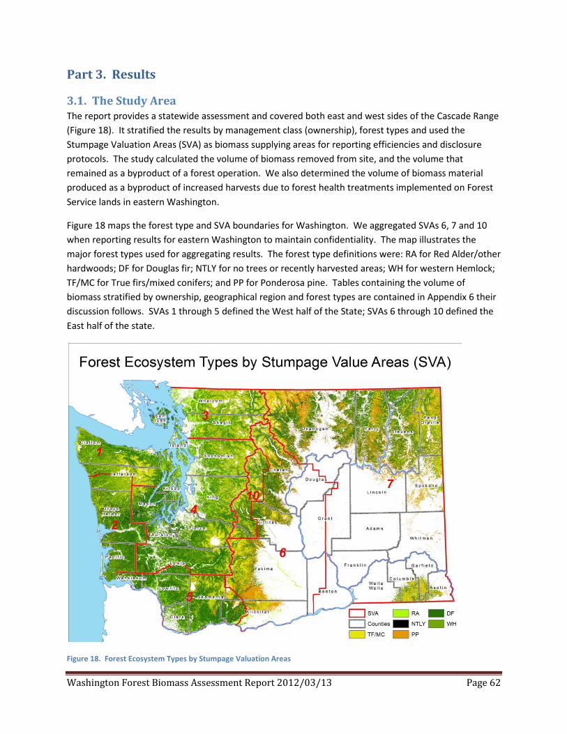
Washington Forest Biomass Assessment Report 2012/03/13 Page 62
Part 3. Results
3.1. The Study Area The report provides a statewide assessment and covered both east and west sides of the Cascade Range (Figure 18). It stratified the results by management class (ownership), forest types and used the Stumpage Valuation Areas (SVA) as biomass supplying areas for reporting efficiencies and disclosure protocols. The study calculated the volume of biomass removed from site, and the volume that remained as a byproduct of a forest operation. We also determined the volume of biomass material produced as a byproduct of increased harvests due to forest health treatments implemented on Forest Service lands in eastern Washington.
Figure 18 maps the forest type and SVA boundaries for Washington. We aggregated SVAs 6, 7 and 10 when reporting results for eastern Washington to maintain confidentiality. The map illustrates the major forest types used for aggregating results. The forest type definitions were: RA for Red Alder/other hardwoods; DF for Douglas fir; NTLY for no trees or recently harvested areas; WH for western Hemlock; TF/MC for True firs/mixed conifers; and PP for Ponderosa pine. Tables containing the volume of biomass stratified by ownership, geographical region and forest types are contained in Appendix 6 their discussion follows. SVAs 1 through 5 defined the West half of the State; SVAs 6 through 10 defined the East half of the state.
Figure 18. Forest Ecosystem Types by Stumpage Valuation Areas

Washington Forest Biomass Assessment Report 2012/03/13 Page 63
3.2. Defining Timber Harvest Level Outlooks Our first step in determining sustainable biomass supply was to consider timber harvest activities. We developed harvest activity using historical trends, accounting for owners, management classes and zones as described in Part 2.4.2. Retention levels in different management zones were simulated using those commercial thinning and regeneration harvest activities that were described in Part 2.4.3.
We developed three harvest outlooks over time that reflected our views of a conservative (low harvest level) outlook, mid-range and aggressive (high harvest level) outlook. The outlooks were guided principally by historical harvest levels. The conservative, mid-range and aggressive harvests are based on 10 year historic levels at the county and owner class level with conservative being the lowest amount of timber that was harvested in a single year from a county by a specific owner class summed up for the state. The mid-range and aggressive harvests follow suit. These outlooks are produced in Figure 19. The harvest volume measured was the merchantable volume on site, not including the breakage and defect component.
The three scenarios encompassed the high and low ranges of historical harvest levels. The conservative harvest outlook produced harvest levels slightly above 2 BBF annually from 2015 through 2030. This outlook constrained merchantable timber production to levels observed in today’s low markets, due mainly to the most current economic recession. The mid-range outlook raised harvest levels to 3 BBF by 2015 and maintained them there for the next three five-year periods. It reflected a conservative recovery from current economic conditions by 2015 by increasing harvest levels in response to greater demand from a recovering economy. The aggressive outlook raised timber harvest levels to nearly 4 BBF over the next 5-year period, and maintained them at around 3.5 BBF for the next 3 five-year periods. This outlook was constructed to mimic an optimistic economic recovery. The greatest difference in timber harvest levels occurs in 2015, when the outlook for timber harvest levels doubled from their conservative outlook counterpart.
Figure 19. Harvest outlooks studied in the assessment
0.0
0.5
1.0
1.5
2.0
2.5
3.0
3.5
4.0
4.5
2010 2015 2020 2025 2030
Mer
chan
tabl
e Ha
rves
t Vol
ume
(BBF
)
Aggressive
MidRange
Conservative
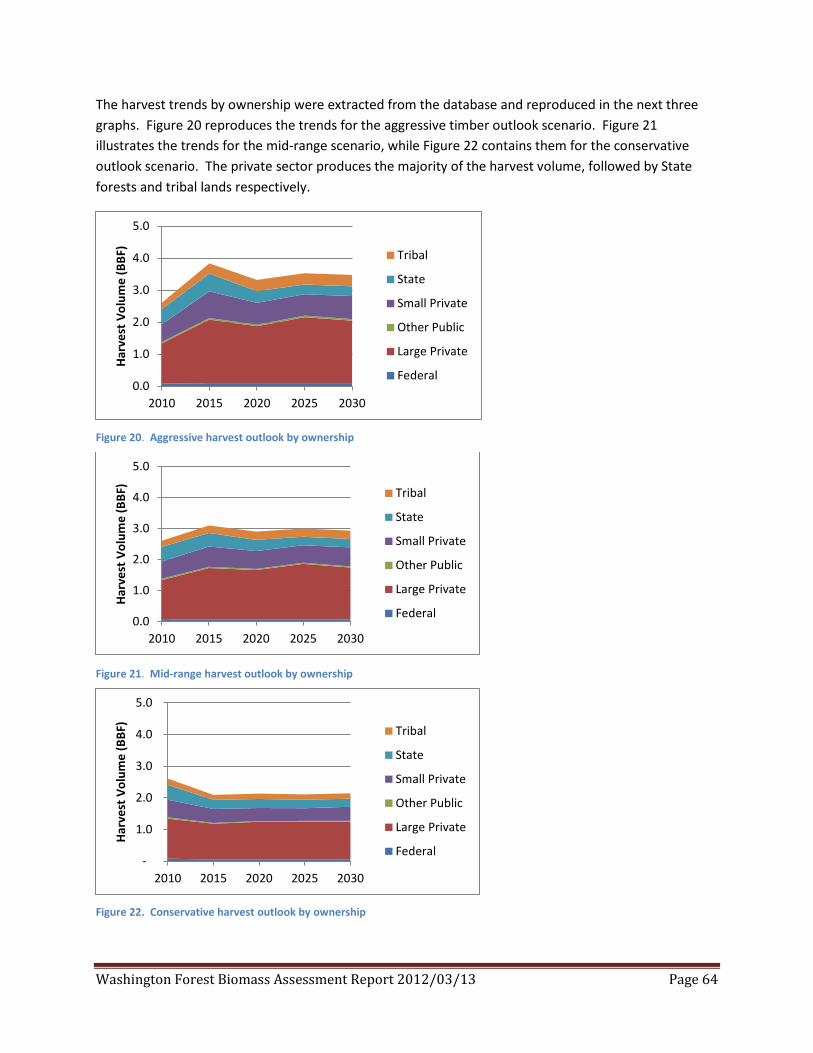
Washington Forest Biomass Assessment Report 2012/03/13 Page 64
The harvest trends by ownership were extracted from the database and reproduced in the next three graphs. Figure 20 reproduces the trends for the aggressive timber outlook scenario. Figure 21 illustrates the trends for the mid-range scenario, while Figure 22 contains them for the conservative outlook scenario. The private sector produces the majority of the harvest volume, followed by State forests and tribal lands respectively.
Figure 20. Aggressive harvest outlook by ownership
Figure 21. Mid-range harvest outlook by ownership
Figure 22. Conservative harvest outlook by ownership
0.0
1.0
2.0
3.0
4.0
5.0
2010 2015 2020 2025 2030
Harv
est V
olum
e (B
BF)
Tribal
State
Small Private
Other Public
Large Private
Federal
0.0
1.0
2.0
3.0
4.0
5.0
2010 2015 2020 2025 2030
Harv
est V
olum
e (B
BF)
Tribal
State
Small Private
Other Public
Large Private
Federal
-
1.0
2.0
3.0
4.0
5.0
2010 2015 2020 2025 2030
Harv
est V
olum
e (B
BF)
Tribal
State
Small Private
Other Public
Large Private
Federal

Washington Forest Biomass Assessment Report 2012/03/13 Page 65
3.3. Forest Biomass Creating harvest outlooks were the first step to calculate the volume of biomass produced as a byproduct of forest operations. Tables describing the data on biomass are found in Appendix 6. A short description of these data at each stage of biomass accounting is presented next.
3.3.1. Post-timber Harvest Biomass The post-timber harvest biomass volumes associated with each harvest scenario were calculated (see Section 2.2.4) and are presented with the next three graphs (Figures 23-25). The trends observed for the post-timber harvest biomass were similar to the harvest outlook trends due to the strong correlation between biomass and harvest volumes. For 2010, the total post-timber harvest biomass for all ownership classes is 4.4 million (MM) BDT, increasing by 2015 to 6.5 MM BDT under the aggressive timber harvest outlook, 5.2 MM BDT under the mid-range outlook, and dropping to 3.6 MM BDT under the conservative outlook.
Figure 23. Post-timber harvest biomass by ownership under the aggressive harvest outlook
Figure 24. Post-timber harvest biomass by ownership under the mid-range harvest outlook
0.0
1.0
2.0
3.0
4.0
5.0
6.0
7.0
2010 2015 2020 2025 2030
Post
Tim
ber H
arve
st B
iom
ass
(M
illio
n BD
T)
Tribal
State
Small Private
Other Public
Large Private
Federal
0.0
1.0
2.0
3.0
4.0
5.0
6.0
7.0
2010 2015 2020 2025 2030
Post
Tim
ber H
arve
st B
iom
ass
(M
illio
n BD
T)
Tribal
State
Small Private
Other Public
Large Private
Federal

Washington Forest Biomass Assessment Report 2012/03/13 Page 66
Figure 25. Post-timber harvest biomass by ownership under the conservative harvest outlook
In order to compare the post-timber harvest biomass estimates from the calculations to data developed from field surveys and interviews with forest owners and biomass processors, we calculated the ratio of the volume of post-timber harvest biomass and the merchantable timber volume in BDT per MBF of timber. The ratio measured the volume contained in stem defect, branches and tops, which were not considered merchantable forest products, to the volume of merchantable timber removed. The ratios are presented here and discussed in Part 4 of the report.
The ratio calculated using the biomass assessment database mid-range harvest scenario was relatively constant over time and within each ownership group, with the exception of Forest Service lands (Table 17). Forest Service ratios were the highest, ranging from 1.56 BDT of biomass per MBF of harvest volume to 1.79 BDT per MBF. Other ownerships including private, state and tribal had a range of 1.19 BDT per MBF to 1.43 BDT per MBF. Relatively speaking, the ratios indicated Forest Service harvest operations contained a higher proportion of branches and tops to commercial product volumes than other ownership groups in our simulations.
Table 17. BDT per MBF metrics using post-timber harvest biomass volume
Year Federal Large Private Other Public Small Private State Tribal 2010 1.79 1.42 1.37 1.33 1.30 1.29 2015 1.68 1.43 1.34 1.35 1.27 1.21 2020 1.59 1.41 1.37 1.34 1.26 1.23 2025 1.56 1.43 1.29 1.32 1.34 1.19 2030 1.59 1.37 1.32 1.33 1.27 1.23 Source: Biomass database
Values are influenced by the volume of branches and tops associated with trees harvested and vary as tree characteristics vary. A higher proportion of branches and tops may be due to stand conditions such as a larger proportion of trees in older age classes. Database harvesting protocols were changed for
0.0
1.0
2.0
3.0
4.0
5.0
6.0
7.0
2010 2015 2020 2025 2030
Post
Tim
ber H
arve
st B
iom
ass
(M
illio
n BD
T)
Tribal
State
Small Private
Other Public
Large Private
Federal

Washington Forest Biomass Assessment Report 2012/03/13 Page 67
Forest Service lands to explore the issue. We used Stand Density Index (SDI) directly to constrain where harvests on Forest Service ownerships took place instead of our default per acre volume harvest criterion. However, the use of SDI did not change the calculated ratio substantially.
3.3.2. Harvested Biomass Harvested biomass was created when harvest configuration constraints were placed on post-timber harvest biomass volumes (see section 2.2.6). The harvest configuration constraints consisted of slope conditions and whether whole tree logging and tops were moved to landings and roadside, or not. Slope constraints were implemented by using either ground-skidding equipment or cable yarding, as described previously. These constraints differed by ownership and forest type. Figures 26-28 depict the trends over time for the aggressive, mid-range and conservative harvest outlooks respectively by ownership.
Harvest configuration reduced the volume of post-timber biomass that can potentially reach markets by 33% suggesting a significant portion of the biomass created by harvest activities remained scattered within the unit due to slope and equipment restrictions, and merchandizing decisions.
Total harvested biomass from all ownerships in 2010 was calculated at 3.0 MM BDT, increasing by 2015 to 4.5 MM BDT in the aggressive timber harvest outlook, 3.5 MM BDT in the mid-range outlook, and decreasing to 2.4 MM BDT in the conservative outlook.
Figure 26. Harvested biomass volume by ownership under the aggressive harvest outlook
0.00.51.01.52.02.53.03.54.04.55.0
2010 2015 2020 2025 2030
Harv
este
d Bi
omas
s (M
illio
n BD
T)
Tribal
State
Small Private
Other Public
Large Private
Federal

Washington Forest Biomass Assessment Report 2012/03/13 Page 68
Figure 27. Harvested biomass volume by ownership under the mid-range harvest outlook
Figure 28. Harvested biomass volume by ownership under the conservative harvest outlook
BDT per MBF ratios using harvested biomass volumes were calculated in a manner similar to that for post-timber harvest biomass using the mid-range harvest scenario. These ratios measured the amount of biomass brought to landings and roadside, with a potential to reach markets given favorable operability conditions, as a function of harvest volume. We considered these ratios to be an upper bound to BDT per MBF ratios that biomass processors and forest owners might use in their assessment work. The ratio represented ideal conditions in which operability and cost constraints had little influence in the production of harvested biomass. Statewide, among all ownerships, an average of 0.92 BDT of harvested biomass were produced for each MBF of merchantable timber harvest (Table 18).
0.0
0.5
1.0
1.5
2.0
2.5
3.0
3.5
4.0
4.5
5.0
2010 2015 2020 2025 2030
Harv
este
d Bi
omas
s (M
illio
n BD
T)
Tribal
State
Small Private
Other Public
Large Private
Federal
0.00.51.01.52.02.53.03.54.04.55.0
2010 2015 2020 2025 2030
Harv
este
d Bi
omas
s (M
illio
n BD
T)
Tribal
State
Small Private
Other Public
Large Private
Federal

Washington Forest Biomass Assessment Report 2012/03/13 Page 69
Table 18. BDT per MBF metrics using harvested biomass volume
Year Federal Large Private Other Public Small Private State Tribal 2010 1.23 0.95 0.94 0.89 0.88 0.87 2015 1.15 0.96 0.90 0.91 0.86 0.81 2020 1.09 0.95 0.91 0.90 0.85 0.83 2025 1.07 0.96 0.86 0.88 0.91 0.80 2030 1.09 0.92 0.88 0.89 0.85 0.83
Source: Biomass database
3.3.3. Potential Market Biomass Operability constraints reduced the amount of harvested biomass that potentially was loaded onto a truck or van. Forest roads conditions, for example, restricted the ability to take what is delivered to the roadside or landing, so there was some portion of harvested biomass that was not processed. These operability constraints reduced the volume by 53% of harvested biomass that had been brought to the roadside or landings and were potentially marketed. Figures 29-31 present the trends in potential market biomass over time by ownership under the three harvest outlooks.
Potential market biomass from all ownerships in 2010 was calculated at 1.4 MM BDT, increasing by 2015 to 2.1 MM BDT in the aggressive timber harvest outlook, 1.6 MM BDT in the mid-range outlook, and decreasing to 1.1 MM BDT in the conservative outlook.
Figure 29. Potential market biomass volume by ownership under the aggressive harvest outlook
0.0
0.5
1.0
1.5
2.0
2.5
2010 2015 2020 2025 2030
Pote
ntia
l Mar
ket B
iom
ass
(Mill
ion
BDT)
Tribal
State
Small Private
Other Public
Large Private
Federal

Washington Forest Biomass Assessment Report 2012/03/13 Page 70
Figure 30. Potential market biomass volume by ownership under the mid-range harvest outlook
Figure 31. Potential market biomass volume by ownership under the conservative harvest outlook
BDT per MBF ratios using potential biomass as the numerator measured biomass recovery that has the potential to be loaded onto a truck or van relative to the timber volume in the harvest unit (Table 19). The potential market volume represents the volume that became accessible to a processor and might be removed from the site under favorable economic conditions. Table 19 presents these ratios for the mid-range harvest scenario. Statewide, an average of 0.44 BDT of biomass was brought to landings and roadside with the potential for loading onto trucks for every MBF of timber harvest volume across management type and over the period 2010 to 2030 under the midrange harvest scenario.
0.0
0.5
1.0
1.5
2.0
2.5
2010 2015 2020 2025 2030
Pote
ntia
l Mar
ket B
iom
ass
(Mill
ion
BDT)
Tribal
State
Small Private
Other Public
Large Private
Federal
0.0
0.5
1.0
1.5
2.0
2.5
2010 2015 2020 2025 2030
Pote
ntia
l Mar
ket B
iom
ass
(Mill
ion
BDT)
Tribal
State
Small Private
Other Public
Large Private
Federal

Washington Forest Biomass Assessment Report 2012/03/13 Page 71
Table 19. BDT per MBF metrics using potential market biomass volume
Year Federal Large Private Other Public Small Private State Tribal 2010 0.45 0.46 0.41 0.44 0.34 0.43 2015 0.41 0.48 0.42 0.44 0.31 0.39 2020 0.40 0.47 0.44 0.43 0.32 0.42 2025 0.39 0.48 0.40 0.42 0.35 0.41 2030 0.40 0.46 0.41 0.42 0.32 0.42
Source: Biomass database
3.3.4. Market Biomass The volume of potential market biomass that was loaded and transported to a facility depended on the set-up cost, the cost of processing and transporting the material to a facility and the market price (see section 2.2.13). We examined a range of costs and market prices to establish boundaries for market biomass supply (Table 20). The medium cost level was determined by employing average responses from our survey and interviews with processors and haulers. The low and high cost levels were determined using 20% below and above the medium level, respectively.
Table 20. Three cost levels for set-up, processing and loading, and hauling used to determine market biomass volumes
Cost Level Mobilization Costs ($/hour)
Processing and Loading Costs ($/ton)
Hauling Costs ($/hr)
Low $90 $21 $76 Medium $120 $26 $95 High $144 $31 $114 Source: Developed for biomass database from survey responses

Washington Forest Biomass Assessment Report 2012/03/13 Page 72
3.4. Determining Fuel Sheds for Existing Facilities For this task, we first identified the location of existing facilities. Once located, we used the residual value to the landowner, that is, the difference between market price and cost, to determine whether the volume of potential market biomass was processed, loaded and transported to the facility. When the residual value was positive, that is, market price was higher than production cost, potential market biomass was processed into market biomass. When the residual value was zero or negative, the potential market biomass was not processed and remained on site.
Figure 32 illustrates the fuel shed for an existing facility located in Tacoma, Washington. Each panel in Figure 32 contains colored parcels that had a positive residual value to the landowner. The progression of the fuel shed was mapped by increasing the market price, and is shown in panels moving from left to right, and top to bottom. At $100 market price, (lower, right panel) the facility’s potential fuel shed extended throughout most of western Washington, and encroached into eastern Washington. The map was produced using the medium cost level assumptions for 2010 harvest levels. Fuel sheds for all existing facilities are provided in Appendix 7.

Washington Forest Biomass Assessment Report 2012/03/13 Page 73
Figure 32. The expansion of a facility’s fuel shed as market price increased under medium cost level for 2010

Washington Forest Biomass Assessment Report 2012/03/13 Page 74
The findings represented in Figure 32 were supported by the responses from biomass operators. The sourcing area for biomass from forest operations varied considerably in relationship to facility proximity to forest operations, feedstock volume requirements, as well as alternatives to burning woody biomass material to generate heat/steam and power. In general, the range of sourcing area in miles radiating from facilities was from 30 miles to as much as 125 miles, one way haul distance (per interviews with fiber procurement managers). The estimated average one-way haul distance weighted by woody biomass fuel volumes consumption was 55 miles, one-way.
3.4.1. Examining Competitive Conditions In reality, a fuel shed for an existing facility is bounded by fuel sheds for nearby facilities. We used the amount of residual value to landowners to discern the facility that would receive biomass from the landowner. A facility received biomass from parcels with residual values that were higher than the residual value calculated for a competing facility. If the residual value for a parcel in Grays Harbor County destined for Longview Fiber was $20 per BDT, and the residual value for the same parcel destined for the Simpson Tacoma Craft facility was $21 per BDT, the biomass would be assigned to the Simpson Tacoma Craft facility.
Biomass fuel sheds for existing facilities were mapped using the definition of competition and are presented in Figures 33, 34 and 35. Competition here is described as the decision of a land owner to sell biomass to more than one facility. With only a single facility in existence a landowner has no choice but to sell to that facility. With additional choices, competition will allow the landowner to sell to the facility that pays the most. The maps illustrate the low, medium and high cost models. Since the maps show results for 2010, the harvest level does not change in the different cost model. Comparing the three figures, one can see that cost level affected the volume of market biomass. In Figure 33, at the low cost level, competition between facilities was evident at $35 and $40 per ton. The maps with medium and high cost levels (Figures 34 and 35 respectively) showed little or no competitive effects (i.e. the filling out of areas surrounding facilities with colored pixels), since costs were high enough to limit the volume of potential market biomass reaching markets. With the medium cost level, a market price of $50 per BDT and with high cost level the market price of $60 per BDT are high enough to extract potential market biomass from the woods and potentially limit supplies to a significant number of individual facilities if their demand is high enough.

Washington Forest Biomass Assessment Report 2012/03/13 Page 75
Figure 33. Market biomass fuelsheds under low cost at varying market prices for all exisiting facilities

Washington Forest Biomass Assessment Report 2012/03/13 Page 76
Figure 34. Market biomass fuelsheds under medium cost at varying market prices for all exisiting facilities

Washington Forest Biomass Assessment Report 2012/03/13 Page 77
Figure 35. Market biomass fuelsheds under high cost at varying market prices for all exisiting facilities

Washington Forest Biomass Assessment Report 2012/03/13 Page 78
Each fuel shed map was transformed into a supply function that related the volume of biomass supply with a market price (Figure 36). Several facilities such as #2, #3, and #11 were among others that had fairly steep curves. These facilities are located in areas where supply was restricted by cost and/or competition from other facilities. There are other facilities, such as #8 and #14, where the competition does not affect supply, and production cost to process and delivered biomass was not a factor until after substantial volumes were consumed.
Figure 36. Supply curves for existing facilities by ID number showing different quantities availability with price changes
3.4.2. Aggregating the Supply of Market Biomass Aggregated market biomass was defined by altering the cost level and market price, using the volume of potential market biomass with positive residual value, and allocating market biomass to the facility with the highest residual value. We found market biomass supply to be fairly elastic at market prices below $50 per BDT for the first 1 MM BDT, 1.5 MM BDT and 1.8 MM BDT under the conservative, midrange and aggressive harvest outlooks respectively (Figure 37). Afterwards availability of market biomass was constrained by competition, and prices increased rapidly. Also, the effect of cost on the aggregate supply curve was as expected. Higher costs were met by higher market prices at a given volume (Figure 38). A 20% change in costs led to slightly higher percent change in price when measured at around 1 MM BDT level.
$30 $40 $50 $60 $70 $80 $90
$100 $110
0 50 100 150 200 250
Mar
ket P
rice
($/B
DT)
1000 BDT by facility
1 2 3 4 5 6 7 8
9 10 11 12 13 14 15

Washington Forest Biomass Assessment Report 2012/03/13 Page 79
Figure 37. Aggregate supply in 2015 using medium cost level at different harvest outlook levels
Figure 38. Aggregate supply in 2015 using Midrange harvest outlook at different cost levels
3.5. Studying Forest Service Eastside Forest Health & Fuels Treatments Forest health and wildfire fuels reduction on federal lands has been an evolving theme of management in response to widespread forest damage in recent decades. Federal land management activity has, as elsewhere in the state, been reduced substantially from its peak in the mid-1980s. A focus on restoration-oriented management and collaborative decision making have increased public consensus and begun to stabilize the federal land management framework in dry forests. Recently, both the Okanogan Wenatchee National Forest and the Colville National Forest have received national recognition and supplemental funding to implement broad-scale forest restoration strategies that were developed with the assistance of non-federal partners. These strategies will be implemented over the
$-
$20
$40
$60
$80
$100
$120
0.0 0.5 1.0 1.5 2.0 2.5
Mar
ket P
rice
($/B
DT)
Million BDT
Conservative Midrange Aggressive
0
20
40
60
80
100
120
0.0 0.5 1.0 1.5 2.0
Mar
ket P
rice
($/B
DT)
Million BDT
Low Cost Medium Cost High Cost

Washington Forest Biomass Assessment Report 2012/03/13 Page 80
next decade, and will coincide with revisions to the long-term land and resource management plans ongoing for these two forests as well as the Umatilla National Forest (WA).
The scenarios for estimating biomass availability are therefore designed to “bracket” a wide array of potential management activity levels. However, standard constraints and assumptions discussed elsewhere in this report all remain applicable to these scenarios, such as the application of harvest scenarios only to non-reserved areas as defined by current management plans (see section 2.2.3), the use of existing transportation systems, and customized operability constraints for each land management class (see section 2.2.7).
3.5.1. Commercial and Noncommercial Harvest Scenarios We examined three scenarios where forest health and fuels treatments were prescribed on USFS lands in eastern Washington. A Baseline scenario harvested approximately 70 MM board feet across the Okanogan-Wenatchee, Colville and Umatilla (WA) National Forests in eastern Washington annually and reflects current commercial harvest activity. An Increased Acres run doubled the harvest levels to about 140 MM board feet per year, whereas the Aggressive run tripled the commercial harvest activity to around 210 MM board feet per year.
The assessment also accounts for baseline and increased noncommercial fuels treatments separately from commercial harvest activities. The noncommercial fuels treatments were identified as stand-alone acres; acres that did not remove any commercial timber volume. Acre targets were used to define the stand-alone, noncommercial fuel treatment acres beginning with a Baseline run figure of 6,400 acres. The Increased and Aggressive runs treated 12,600 and 19,100 acres, respectively.
We used two prescriptions separately to examine the impact of forest health treatments on biomass supply with commercial harvest activity: a light thinning regime that removed only material up to a 12 inch diameter limit, and a heavy thinning treatment that reduced stand basal area to 45 square feet per acre. Both prescriptions were run separately within stands that comprised the commercial timber volume portion of the scenario. An individual project designed by the Forest Service would use some combination of treatment prescriptions that generally fall between these two in terms of their intensity. Completing separate scenarios with both sets of prescriptions serves to provide a reasonable range of the potentially available biomass material. Noncommercial fuel treatment stands were managed using only the light thinning regime prescription, removing no commercial material.
Under the baseline scenario, the commercial harvest of about 70 MM bf was met using 10,600 acres under the light thinning regime and 6,600 acres under the heavy thinning regime. The Increased run required 21,000 and 12,700 acres to meet the 140 MM bf harvest level using the light and heavy thin prescriptions respectively. The Aggressive run harvested 50,000 and 37,800 acres to meet the 210 MM bf annual harvest level, respectively. All treatments used a 50% operability percentage for federal ownership (see section 2.2.7).
Finally, a proximity measure was used to target the highest density and volume stands around developed areas first as indicated by land-use information in the land parcel database. The proximity

Washington Forest Biomass Assessment Report 2012/03/13 Page 81
measure mimics fuel treatment activities that occur along the urban to wildland gradient, targeting those acres that potentially have the highest benefits first.
3.5.2. Noncommercial Treatment Harvesting Costs For harvest activity estimated elsewhere in this report, the two cost components modeled for commercial harvests are applied as described in section 2.2.10. In estimating material from stand-alone noncommercial forest health and fuels treatments it was necessary to define additional biomass harvesting costs since biomass removal for these acres would incur an additional cost of bringing material to the roadside. In a commercial harvest operation, biomass was brought to the roadside along with the timber without the need to utilize additional equipment. For stand-alone acres, the lack of commercial activity precluded any harvest operations used to bring out material to the roadside. Biomass harvesting costs were added to compensate for the lack of any harvest configuration associated with stand-alone acres.
We therefore define the additional cost of biomass harvesting using three levels: $30 per BDT, $45 per BDT and $60 per BDT. The three cost levels were determined after consulting Schiess and Yonaka (1982) and interviews with operators. These three cost levels represent the cost incurred when employing equipment, such as a bundler or skidder, to pull biomass to the roadside. Each of the three cost levels was associated with the low, medium and high cost equations respectively that were develop for biomass production associated with commercial harvest activities and described in Section 2.2.10. This method results in a much lower proportion of potential market biomass than would be found in other treatments, however it best approximates current and likely future federal land forest health management activity associated with stand-alone treatments.
3.5.3. Results We report the levels of biomass produced under the Baseline, Increased and Aggressive runs for the two prescriptions. We start by reporting the levels of post-timber harvest biomass produced under each scenario, and continue with the results for harvested biomass and potential market biomass. Finally, the report presents the market biomass and supply curves associated with the two levels of prescriptions.
Figures 39 through 41 present the biomass produced as a result of augmenting the treatment areas for federal forests in eastern Washington for 2015 through 2030. These figures portray the production volume under the light thinning regime: removal of trees less than 12 inches in diameter.

Washington Forest Biomass Assessment Report 2012/03/13 Page 82
Figure 39. Forest Service production of Post-Timber Harvest Biomass under three levels of harvest activity under a light thinning regime.
Figure 40. Forest Service production of Harvested Biomass under three levels of harvest activity under a light thinning regime.
0
100,000
200,000
300,000
400,000
500,000
600,000
2015 2020 2025 2030
BDT
Year
Baseline
Increased
Aggressive
0
100,000
200,000
300,000
400,000
500,000
600,000
2015 2020 2025 2030
BDT
Year
Baseline
Increased
Aggressive

Washington Forest Biomass Assessment Report 2012/03/13 Page 83
Figure 41. Forest Service production of Potential market biomass under three levels of harvest activity under a light thinning regime.
Biomass production levels from post-timber harvest to potential market biomass replicate the scenario assumptions of doubling and tripling the activity levels in these national forests. In general, the Increased run produced biomass levels twice as large as the Baseline run; the Aggressive run produced biomass levels three-times as large as the Baseline run. Potential market biomass is about 1/3 of the harvested biomass, since operability constraints continue to limit the volume accessible to markets. Based on the treatment prescription, harvest systems and forest types, average per acre volumes of post-timber harvest biomass was calculated as 15 BDT per acre.
A result similar to the above was obtained under the heavy thinning regime; reducing basal area to 45 square feet per acre. Figures 42 through 44 illustrate the results. The amount of biomass produced was slightly lower than under the thinning regime since less acres were commercially harvested to reach the timber harvest levels of 70, 140 and 210 MM board feet under the baseline, Increase and Aggressive runs. Based on the treatment prescription, harvest systems and forest types, average per acre volumes of post-timber harvest biomass was calculated at 21 BDT per acre.
0
100,000
200,000
300,000
400,000
500,000
600,000
2015 2020 2025 2030
BDT
Year
Baseline
Increased
Aggressive

Washington Forest Biomass Assessment Report 2012/03/13 Page 84
Figure 42. Forest Service production of Post-Timber Harvest Biomass under three levels of harvest activity under a heavy thinning regime.
Figure 43. Forest Service production of Harvested Biomass under three levels of harvest activity under a heavy thinning regime.
0
100,000
200,000
300,000
400,000
500,000
600,000
2015 2020 2025 2030
BDT
Year
Baseline
Increased
Aggressive
0
100,000
200,000
300,000
400,000
500,000
600,000
2015 2020 2025 2030
BDT
Year
Baseline
Increased
Aggressive
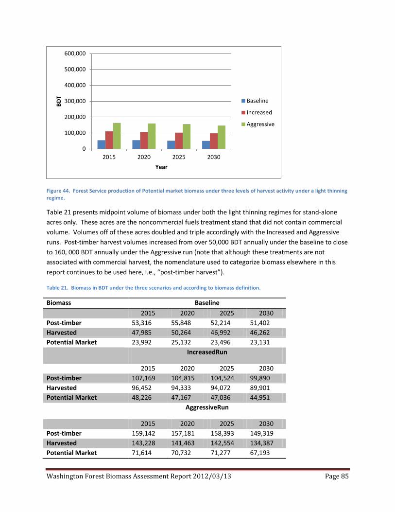
Washington Forest Biomass Assessment Report 2012/03/13 Page 85
Figure 44. Forest Service production of Potential market biomass under three levels of harvest activity under a light thinning regime.
Table 21 presents midpoint volume of biomass under both the light thinning regimes for stand-alone acres only. These acres are the noncommercial fuels treatment stand that did not contain commercial volume. Volumes off of these acres doubled and triple accordingly with the Increased and Aggressive runs. Post-timber harvest volumes increased from over 50,000 BDT annually under the baseline to close to 160, 000 BDT annually under the Aggressive run (note that although these treatments are not associated with commercial harvest, the nomenclature used to categorize biomass elsewhere in this report continues to be used here, i.e., “post-timber harvest”).
Table 21. Biomass in BDT under the three scenarios and according to biomass definition.
Biomass Baseline 2015 2020 2025 2030 Post-timber 53,316 55,848 52,214 51,402 Harvested 47,985 50,264 46,992 46,262 Potential Market 23,992 25,132 23,496 23,131 IncreasedRun
2015 2020 2025 2030 Post-timber 107,169 104,815 104,524 99,890 Harvested 96,452 94,333 94,072 89,901 Potential Market 48,226 47,167 47,036 44,951 AggressiveRun
2015 2020 2025 2030 Post-timber 159,142 157,181 158,393 149,319 Harvested 143,228 141,463 142,554 134,387 Potential Market 71,614 70,732 71,277 67,193
0
100,000
200,000
300,000
400,000
500,000
600,000
2015 2020 2025 2030
BDT
Year
Baseline
Increased
Aggressive

Washington Forest Biomass Assessment Report 2012/03/13 Page 86
Market biomass was estimated using the three cost scenarios. In addition to the usual costs associated with a commercial forest operation, cost to bundle and pull biomass to the roadside was added to the biomass recovery for stand-alone acres. Biomass recovery costs were not included when commercial harvest operations occurred since their piling and bringing to the roadside occurs with timber yarding.
Figure 45 illustrates the market biomass at varying prices under the baseline run with high, medium and low cost assumptions for the light thinning regime and considers the volumes produced under the commercial and stand-alone treated acres. The breaks in the market supply curves were due to the biomass recovery costs. The cost to bundle and pull to the roadside biomass not associated with a forest operation required a higher market price to clear the market. In the figure, the price necessary to recover the biomass harvest costs under the high cost scenario was greater than $100 per BDT. Under the medium and low cost assumptions, market prices need to increase by approximately $30 and $20 for biomass from stand-alone acres to clear the market. The results show from 1,500 to 28,000 BDT made available at $45 per BDT, depending on cost assumptions. There are about 34,000 to 49,000 BDT made available from national forests under the baseline case, depending on cost assumptions and using a market price of $100 per BDT.
Figure 45. Market biomass supply from national forests in 2015 under the baseline case fpr three cost scenarios using the light thinning regime.
This behavior was replicated in the Increased and Aggressive runs (figures 46 and 47 respectively). The difference was the amount of market biomass made available due to higher treatment and harvest activities. Market biomass availability at $45 per BDT was calculated from 3,000 to 60,000 BDT, and from 67,000 to 100,000 BDT at $100 per BDT. The relationship between the Baseline and Increased run was nearly double the volume.
$-
$20
$40
$60
$80
$100
$120
- 40,000 80,000 120,000 160,000
Mar
ket P
rice/
BDT
BDT
Baselinelightlow BaselineLightMed BaselineLightHigh

Washington Forest Biomass Assessment Report 2012/03/13 Page 87
Figure 46. Market biomass supply from national forests in 2015 under the Increased case fpr three cost scenarios using the light thinning regime.
In figure 47, market biomass availability at $45 per BDT was calculated from 7,300 to 93,000 BDT at $45, and from 102,000 to 152,000 BDT at $100 per BDT. The relationship between the Baseline and Aggressive run was nearly triple the volume.
Figure 47. Market biomass supply from national forests in 2015 under the Aggressive case for three cost scenarios using the light thinning regime.
The forest health runs have the opportunity to contribute additional biomass volumes, but only if market prices reach levels high enough to cover harvesting costs or harvesting costs can be substantially reduced. When treatment occurred in stand-alone acres, costs included additional equipment costs associated with bundling or pulling material to the roadside. Under a high cost scenario, market prices
$-
$20
$40
$60
$80
$100
$120
- 40,000 80,000 120,000 160,000
Mar
ket P
rice/
BDT
BDT
IncreasedLightLow IncreasedLightMed IncreasedLightHigh
$-
$20
$40
$60
$80
$100
$120
- 40,000 80,000 120,000 160,000
Mar
ket P
rice/
BDT
BDT
AgressiveLightLow AggressiveLightMed AggressiveLightHigh

Washington Forest Biomass Assessment Report 2012/03/13 Page 88
needed to bring materials from stand-alone acres were above $100 per BDT. A medium cost scenario suggested market prices above $80 per BDT. A low cost scenario had prices at $60.
Part 4. Sustainability The project goals were to 1) calculate and characterize the volume of biomass removed from site, i.e., market biomass, stratified by ownership, species and time, and 2) assess its availability. The study team was also asked to calculate and characterize the volume retained on site, i.e., residual biomass, as the byproduct of a forest operation. The successful establishment and maintenance of regional bioenergy supply systems that utilize biomass from forest operations requires a broad understanding of potential benefits and impacts of forest biomass harvest activities. An understanding of the effect of varying levels of biomass left for ecosystem functions is central to developing a forest-based bio-resource for the developing bioenergy market.
Residual biomass is described in section 4.1 of the report. Residual biomass is composed of the sum of residual harvested biomass, residual potential market biomass and residual market biomass produced as a byproduct of a forest operation. We also present a range of volume of woody material that pre-existed the forest operation. While the study makes broad but reasonable assumptions about the adequacy of harvest residuals and pre-existing biomass to meet ecological function requirements, a more detailed analysis of site-specific retention needs is being completed separately from this study, in the context of Washington State forest practices regulations.
In section 4.2 the study presents metrics to determine whether our use of a statewide database to simulate landowner behavior was consistent with information gathered from individuals and organizations that operate at the local scale. We discuss their differences, suggest ways to improve the information collected and recommend areas of future work in this part of the study. Section 4.3 describes the characteristics of biomass. Section 4.3 contains a review of literature on ecological retention. It produces a synthesis of existing literature useful to understand the context of ecological retention within the supply of market biomass framework developed here. Section 4.4 provides a discussion of market sustainability.
4.1. What Volume of Forest Biomass Is Left on Site? There are two sources of biomass retained on site: pre-existing material and the residual volumes presented in Part 3 as the byproduct of a forest operation. This section first discusses the volumes of material that were produced as a byproduct of a forest operation. We then present a range of values for pre-existing material. The sum of these two components characterizes the volume of forest biomass left on site after timber harvest and biomass collection.
4.1.1. Material Produced as a Byproduct of a Forest Operation Since favorable conditions to extract woody material from a harvest unit were not always present, some amount of biomass was left behind as a byproduct of the forest operation. When harvest configurations such as delimbing or removing tops at the place where the tree was harvested were used, the biomass contained in these components was left behind scattered throughout the harvest unit. When road

Washington Forest Biomass Assessment Report 2012/03/13 Page 89
conditions in sections of a harvest unit did not permit a grinder, truck or van to maneuver, those piles were not processed and the associated biomass remained on site. Even when tops and branches were yarded to a landing, and were it possible to set up a grinder and chip van at the pile, a portion of the biomass remained on site due to low market prices or insufficient volume to economically haul the material to a facility. Table 22 summarizes the progression of biomass produced as a byproduct of a forest operation as estimated by this assessment.
Table 22. The distribution of biomass in million BDT according to the naming convention used in this study (see Figure 2)
Post-timber Harvest Biomass Harvested Biomass Potential Market Biomass EAST 1.067 0.694 0.282 WEST 3.382 2.289 1.107 TOTAL 4.449 2.983 1.389 Source: Biomass database; reference year 2010
Of the 4.4 million BDT of post-timber harvest biomass, 3.0 million BDT are delivered to the roadside under the 2010 harvest level outlook. A change in the harvest configuration may change the amount of post-timber harvest biomass reaching the landing or roadside, but the change in this volume will be limited to a certain extent by topography. Of this 4.4 million BDT, 1.4 million BDT (33%) were left scattered.
The operability that roads and equipment permit at the landing and roadside also results in biomass remaining behind. This volume is the difference between the harvested and potential market biomass, and amounted to 1.6 million BDT. Changing patterns in equipment use from today’s practices to alternatives allowing greater operability will change the amount potentially loaded on the truck and removed from site. Such changes will reduce the amount of residual biomass left at the roadside and landings.
Finally, current cost and market prices influence the amount of potential market biomass delivered to a facility. This volume was estimated between 440,000 and 560,000 BDT in 2010. Changes in market prices, driven by an increase in demand for example, will increase the amount of potential biomass that reaches a facility. At prices near $100 per BDT, an estimated 1.3 million BDT, of the 1.4 million BDT of potential market biomass, could be delivered to facilities. Of the 1.4 million BDT, around 100,000 BDT would remain. Market price and cost improvements are likely to be the most important factor influencing the amount of potential market biomass that would be removed from site. These two factors represent the more important ones that have the ability to influence the volume of biomass brought to a facility in the short term.
Of the total biomass produced as a byproduct of a forest operation, one third of the material was left scattered in the woods since the volume represents defect stem volume, tops and limbs that were not brought to a landing or roadside. This is a lower bound for the volume left scattered, as operability constraints also prevented a portion of the harvested biomass from reaching the landing. The total left behind due to harvest configuration and operability is 69% of the total biomass produced as a byproduct of a forest operation. Based on database calculations, of the total biomass left behind as a byproduct of

Washington Forest Biomass Assessment Report 2012/03/13 Page 90
a forest operation, at least 33% was left scattered in the wood, and at most 66% was brought to the roadside or landing.
4.1.2. The Range of Estimates of Pre-existing Woody Materials Volume For the purposes of this study, pre-existing biomass is the naturally occurring wood that resides in the unit prior to a forest operation. The biomass database does not produce estimates of pre-existing downed wood; hence we used existing tools and database to estimate the potential range of pre-existing woody material volume.
The database comes from the Ohlmann and Waddell (2002) report on using BLM (Bureau of Land Management) and CVS (current vegetation survey) data to estimate the amount of large woody debris (>5”) that was present across the forest types of Washington and Oregon. The tool is the DecAID decayed wood advisor decision support tool that Mellen-McLean et al. (2009) developed using the Ohlmann and Waddell study data to link estimates of woody biomass and snags from inventory data to wildlife habitat needs. That data is collated for forested wildlife habitat regions identified in Johnson and O’Neil (2001) for the PNW region.
Johnson and O’Neil (2001) characterize seven wildlife habitat types (WHT) for Washington State that are covered by forests. Two are exclusively in western Washington, 4 exclusively in eastern Washington, and 1 covering a habitat type found on both sides of the state. These types are: Eastside Mixed Conifer Forest (EMCF) with two sub-regions – the Blue Mountains and Northern Rockies; Ponderosa pine/Douglas-fir Forest – (PP/DF); Lodgepole Pine Forest (LP); Montane Mixed Conifer Forest (MMCF); and Westside Lowland Conifer-Hardwood Forest (WLCHF) with two sub-regions – the West Cascades and coastal areas. They categorize forests into 3 main structural classes for evaluating their usage and effectiveness as wildlife habitat. The classes are open canopy (think recent disturbance, natural or otherwise); small and medium sized trees (as in closed canopy forests in early seral stages) and larger trees (as in older forests with the largest trees that might occur in a given bio-physical envelope).
The DecAID tool provides summaries for the Johnson and O’Neil habitat types and canopy conditions without management and also provides summaries for all forests by habitat and canopy condition. It does not specifically summarize a managed forest condition but broad trends in the data are visible in comparing the two summaries. . For the WHT’s found in Washington downed wood values range from 3-22 m3 per ha > 5” for Eastern Washington and 11-225 m3 per ha > 5” in Western Washington. Those average values by WHT cover an even wider range of values within WHT (0-297 m3 per ha for Eastern Washington, 0-837 m3 per ha for Western Washington). These values represent the best known estimate of pre-existing large woody debris by wildlife habitat type. For that reason we have use the DecAID data as a proxy estimate of the potential amount of pre-existing down wood that might be present on harvested sites, though there is high uncertainty in those estimates.
Appendix 8 provides the distributions of pre-existing wood from DecAID in percent cover for each WHT and structural class (open canopy, small trees, larger trees). Additional charts in Appendix 8 show the BDT associated with each percent cover by each WHT and condition class. The BDT values were derived using the linear regression outputs provided by DecAID to convert percent cover to m3 per ha and then
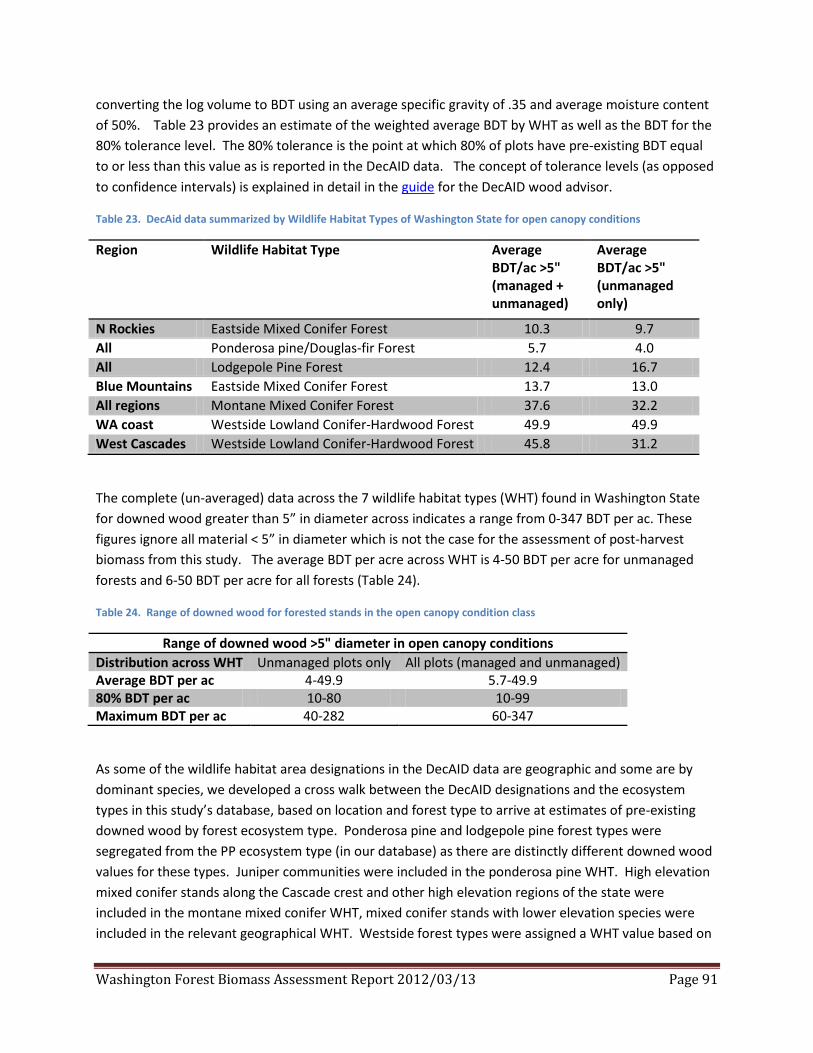
Washington Forest Biomass Assessment Report 2012/03/13 Page 91
converting the log volume to BDT using an average specific gravity of .35 and average moisture content of 50%. Table 23 provides an estimate of the weighted average BDT by WHT as well as the BDT for the 80% tolerance level. The 80% tolerance is the point at which 80% of plots have pre-existing BDT equal to or less than this value as is reported in the DecAID data. The concept of tolerance levels (as opposed to confidence intervals) is explained in detail in the guide for the DecAID wood advisor.
Table 23. DecAid data summarized by Wildlife Habitat Types of Washington State for open canopy conditions
Region Wildlife Habitat Type Average BDT/ac >5" (managed + unmanaged)
Average BDT/ac >5" (unmanaged only)
N Rockies Eastside Mixed Conifer Forest 10.3 9.7 All Ponderosa pine/Douglas-fir Forest 5.7 4.0 All Lodgepole Pine Forest 12.4 16.7 Blue Mountains Eastside Mixed Conifer Forest 13.7 13.0 All regions Montane Mixed Conifer Forest 37.6 32.2 WA coast Westside Lowland Conifer-Hardwood Forest 49.9 49.9 West Cascades Westside Lowland Conifer-Hardwood Forest 45.8 31.2
The complete (un-averaged) data across the 7 wildlife habitat types (WHT) found in Washington State for downed wood greater than 5” in diameter across indicates a range from 0-347 BDT per ac. These figures ignore all material < 5” in diameter which is not the case for the assessment of post-harvest biomass from this study. The average BDT per acre across WHT is 4-50 BDT per acre for unmanaged forests and 6-50 BDT per acre for all forests (Table 24).
Table 24. Range of downed wood for forested stands in the open canopy condition class
Range of downed wood >5" diameter in open canopy conditions Distribution across WHT Unmanaged plots only All plots (managed and unmanaged) Average BDT per ac 4-49.9 5.7-49.9 80% BDT per ac 10-80 10-99 Maximum BDT per ac 40-282 60-347
As some of the wildlife habitat area designations in the DecAID data are geographic and some are by dominant species, we developed a cross walk between the DecAID designations and the ecosystem types in this study’s database, based on location and forest type to arrive at estimates of pre-existing downed wood by forest ecosystem type. Ponderosa pine and lodgepole pine forest types were segregated from the PP ecosystem type (in our database) as there are distinctly different downed wood values for these types. Juniper communities were included in the ponderosa pine WHT. High elevation mixed conifer stands along the Cascade crest and other high elevation regions of the state were included in the montane mixed conifer WHT, mixed conifer stands with lower elevation species were included in the relevant geographical WHT. Westside forest types were assigned a WHT value based on

Washington Forest Biomass Assessment Report 2012/03/13 Page 92
location (county), and where counties could have more than one designation, the species mix of interest. Deciduous types (RA (Red alder) in our database) do not have a separate category in the DecAID database so average values for eastern and western Washington were used to represent these types. Applying the cross walk to all stands in the database that receive a timber harvest in a given year, and using the mid-range harvest scenario generates weighted average estimates of BDT per acre and the 80% tolerance level by forest ecosystem type as shown in Table 25 for Eastside and Westside regions respectively.
Table 25. Average and 80% tolerance level of BDT per acre of pre-existing downed wood >5” in diameter by forest ecosystem type
Forest Ecosystem Type
Average BDT
80% tolerance level BDT
DF 10.6 25.0 PP 9.4 18.9 RA 10.5 24.3 TFMC 14.5 32.0 WH 18.7 38.9 Eastside 11.6 25.8 DF 41.0 85.6 PP 7.5 15.9 RA 37.3 70.6 TFMC 40.4 77.2 WH 41.3 87.3 Westside 40.2 82.6 All areas 29.5 61.4
Using the same mid-range harvest simulation to estimate the harvest area each year, and weighting to all treated stands we can estimate the range of total residual biomass that will result from treatments across time. Figure 48 shows the range of dispersed residual biomass resulting from timber harvest (i.e. never brought to the landing) and Figure 49 shows an additional amount of piled slash that is not removed from the site because of market and technological limitations as modeled for the moderate harvest scenario. On top of each of these modeled estimates of residual biomass arising from harvest is a gradient fill that shows the range of pre-existing biomass up to the 80% tolerance level. This gradient fill can be interpreted as the range of potential pre-existing biomass volumes on sites where treatments were scheduled under the mid-range harvest scenario. It does not include pre-existing biomass on sites that did not get a treatment during the 30 year period.

Washington Forest Biomass Assessment Report 2012/03/13 Page 93
Figure 48. Dispersed biomass estimates for the mid-range harvest scenario plus the residual harvested biomass calculated in the biomass database
Figure 49. Minimum of piles and dispersed biomass estimates for the mid-range harvest scenario (does not include residual market biomass left in piles due to economic constraints)
Using the study’s mid-range harvest scenario, the 80% tolerance limit of pre-existing woody material estimates provided by DecAID, and the study’s technical and economic filters that were used to allocate biomass across its different categories, the study team estimated a minimum of 8.6 MM BDT (in 2010) and a maximum of 11 MM BDT (in 2015) of biomass that were left on harvested sites statewide (Figure 48). The variability in this total pictured in Figure 49 was a mirrored reflection of the mid-range harvest projection used. The minimum tonnage reflected low levels of harvested activity, while the maximum tonnage corresponds to the year of highest harvest activity.
More importantly, the source of greatest variability in Figures 48 and 49 was associated with the pre-existing volume of woody material. The study's calculations show that retained woody biomass immediately following a timber harvest will always add to pre-existing levels. Additional biomass produced as a result of a forest operation in piles and at roadside added 2.4 MM BDT for 2010. This
-
2
4
6
8
10
12
14
2010 2015 2020 2025 2030
Biom
ass
in m
illio
ns o
f BDT
Pre-Existing up to the80% tolerance levelResidual HarvestedBiomass
-
2
4
6
8
10
12
14
2010 2015 2020 2025 2030
Biom
ass
in m
illio
ns o
f BDT
Pre-Existing up to the80% tolerance levelResidual PotentialMarket BiomassResidual HarvestedBiomass

Washington Forest Biomass Assessment Report 2012/03/13 Page 94
value is the sum of residual biomass associated with potential market biomass and market biomass described in Figure 50.
Figure 50. Summary of biomass under the various definitions used in the assessment
4.2. Validating Database Values
4.2.1. Developing BDT per Acre Metrics An assessment of volumes of unprocessed biomass material retained on site after harvest or treatment operations was conducted through consultation with various biomass processing contractors. We used this information to understand and reconcile any differences we observed comparing prior field surveys of piled and dispersed biomass with our calculations above.
Table 26 shows the biomass per acre figures by half-state region, ownership and forest type using the study’s biomass database for the different stages of processing. Using these values the study calculated the volume of biomass retained on site as a byproduct of a forest operation.
Post-timber Harvest Biomass 4.4 MM BDT
F
ores
t Ope
ratio
n
Pre-existing woody material ranges from 0 to 7.2 MM BDT
Merchantable Stem Volume 7.5 MM BDT
Harvested Biomass 3.0 MM BDT
Potential Market Biomass 1.4 MM BDT
Market Biomass 0.6 – 1.3 MM BDT
Residual Harvested Biomass 1.4 MM BDT
Residual Potential Market Biomass 1.6 MM BDT
Residual Market Biomass 0.1 – 0.8 MM BDT

Washington Forest Biomass Assessment Report 2012/03/13 Page 95
Table 26. Per acre biomass estimates calculated using the database.
Post-timber Harvest Biomass (BDT per ACRE) Federal Large Private Other Public Small Private State Tribal Average EAST 22.38 27.52 24.23 26.80 28.54 28.96 26.42
DF 20.00 20.55 26.34 26.40 27.28 26.27 24.10 PP 23.01 23.21 20.33 20.78 24.76 25.89 22.82 RA 20.03 - 17.36 13.32 7.58 15.11 TFMC 24.18 32.91 22.03 29.53 34.59 33.85 29.76 WH 21.69 48.64 56.37 39.98 39.25 43.26 37.76
WEST 24.51 41.18 41.19 39.63 42.61 41.84 39.61 DF 24.69 42.15 36.76 39.89 47.88 19.05 39.94 OP 12.59 15.11 12.59 20.12 18.60 33.04 17.37 RA 18.50 40.08 41.39 41.15 37.56 26.37 37.77 TFMC 22.11 42.20 36.14 32.51 39.71 44.17 36.49 WH 32.03 56.37 58.02 51.53 56.17 66.87 52.83
Harvested Biomass (BDT per ACRE)
Federal Large Private Other Public Small Private State Tribal Average EAST 8.86 11.49 10.85 11.10 11.58 12.09 10.90
DF 7.60 7.97 13.27 10.41 10.70 9.79 9.65 PP 9.65 10.19 9.54 8.85 9.48 10.81 9.58 RA 9.60 - 6.70 4.63 5.76 6.40 TFMC 9.33 13.40 9.02 11.70 15.48 12.74 12.05 WH 8.59 20.81 18.50 18.61 15.85 24.12 16.33
WEST 7.13 17.28 20.93 17.10 16.31 19.24 16.51 DF 7.76 15.58 16.86 14.82 17.77 14.22 15.34 OP 9.50 6.73 9.50 15.05 7.68 24.66 8.53 RA 5.79 15.90 16.97 16.53 14.29 9.66 14.81 TFMC 6.99 17.63 19.22 13.99 14.86 17.94 15.10 WH 7.48 27.84 37.70 27.07 22.30 30.41 24.63
Potential Market Biomass (BDT per ACRE)
Federal Large Private Other Public Small Private State Tribal Average EAST 3.20 4.86 4.54 4.68 4.57 5.52 4.47
DF 3.19 3.35 5.58 4.37 4.07 4.60 4.01 PP 2.99 5.10 4.77 4.42 3.32 5.19 4.14 RA 5.09 - 3.55 1.67 4.09 3.25 TFMC 3.17 4.69 3.16 4.10 6.97 5.10 4.49 WH 3.61 8.74 7.77 7.82 6.02 11.34 6.80
WEST 2.57 8.26 10.53 8.08 5.92 13.49 7.48 DF 2.93 7.75 8.75 7.16 6.52 9.95 7.05 OP 1.14 2.94 4.56 7.22 2.49 17.26 3.53 RA 2.63 7.71 7.24 8.01 5.24 6.86 6.68 TFMC 2.00 7.67 8.78 5.97 5.33 12.56 6.36 WH 2.79 13.90 21.30 13.17 8.18 21.29 11.73
Source: Biomass database DF, Douglas fir; PP, Ponderosa pine; RA, Red Alder/Hardwoods; TFMC, True fir/Mixed conifers; WH, Western hemlock; OP, other pine.
This study’s estimates of biomass production in BDT per acre allow comparison with comparable estimates from other studies. For example, Oneil and Lippke (2009) estimated recoverable biomass

Washington Forest Biomass Assessment Report 2012/03/13 Page 96
from harvest operations in northeastern Washington at 11.4 BDT per acre of recoverable biomass from a total of 26 BDT per acre generated as a byproduct of harvest or treatment operations. Their estimate of recoverable biomass was significantly higher than our average 4.5 BDT per acre potential market biomass, even though their calculation of 26 BDT per acre of biomass generated was similar to this study’s average 26.4 BDT per acre. The difference can be attributed to differences in assumptions. Oneil and Lippke (2009) assumed that all piled material and approximately ½ the dispersed material >5” dbh could be removed under economically favorable conditions. In this study, we assume that no dispersed material is recovered and only a small percent of the piled material is recovered.
An explanation might be found in fluctuations in market conditions, which might change timber harvest levels, equipment configuration and operability constraints. It is possible that market conditions might affect operability constraints, but these changes were not modeled in the present assessment, and were assumed to only operate over a longer term compared to the more rapid effect market price changes might have on the amount of potential market biomass actually removed. Favorable changes in the operability conditions for example, would increase the volume of potential market biomass brought to roadsides and landings. This study, however, assumed that efficiency gains would occur first by improving recovery of market biomass at roadsides and landings, prior to changes in the amount of potential market biomass brought to the roadsides and landings. For example, a type of efficiency gain, such as the way a pile at a landing was constructed, may improve recovery of market biomass, without any additional potential market biomass production.
Table 27 shows the biomass retained on site as a byproduct of a forest operation in BDT per acre calculated using the biomass database. The average volume of biomass retained was 21.95 BDT per acre on the Eastside and 32.14 BDT per acre on the Westside.
Table 27. The distribution of the difference between post-timber harvest biomass and potential market biomass (Biomass retained on site as a byproduct of a forest operation)
Biomass Retained on Site as a byproduct of a forest operation (BDT per ACRE) Federal Large Private Other Public Small Private State Tribal AVERAGE EAST 19.18 22.66 19.69 22.12 23.98 23.43 21.95
DF 16.81 17.21 20.76 22.03 23.22 21.67 20.09 PP 20.02 18.12 15.57 16.36 21.45 20.70 18.68 RA 14.94 - 13.81 11.66 3.49 11.86 TFMC 21.00 28.22 18.87 25.43 27.62 28.75 25.27 WH 18.08 39.90 48.60 32.16 33.23 31.92 30.97
WEST 21.94 32.92 30.66 31.55 36.68 28.35 32.14 DF 21.76 34.40 28.02 32.72 41.36 9.09 32.89 PP 11.45 12.17 8.03 12.90 16.11 15.78 13.85 RA 15.87 32.37 34.15 33.14 32.32 19.51 31.09 TFMC 20.11 34.53 27.36 26.54 34.38 31.61 30.13 WH 29.24 42.47 36.71 38.35 47.99 45.58 41.10
Source: Biomass database. DF, Douglas fir; PP, Ponderosa pine; RA, Red Alder/Hardwoods; TFMC, True fir/Mixed conifers; WH, Western hemlock; OP, other pine.

Washington Forest Biomass Assessment Report 2012/03/13 Page 97
4.2.2. Computing BDT per MBF Metrics The study team assessed values calculated using the study database with similar values derived from interviews and field studies. The interview and field exercises were completed independently; field study values and interview results were completed prior to the database calculations and by different members of the study team. Table 28 shows the BDT per MBF calculated using the biomass database over time and by management type.
Table 28. BDT per MBF values for harvested biomass calculated from the biomass database Year Federal Large Private Other Public Small Private State Tribal 2010 1.23 0.95 0.94 0.89 0.88 0.87 2015 1.15 0.96 0.90 0.91 0.86 0.81 2020 1.09 0.95 0.91 0.90 0.85 0.83 2025 1.07 0.96 0.86 0.88 0.91 0.80 2030 1.09 0.92 0.88 0.89 0.85 0.83
Source: Biomass database
Study interview data were used to develop an estimate of biomass material recovered per MBF of harvested sawlogs and pulp logs and to generate a biomass per acre estimate. The weight of biomass recovered in BDT for each MBF of timber recovered was calculated and measured from data collected from our field interviews, either as scaled volume in MBF or sold by weight. This is a standard metric used in the field to quickly assess potential volumes of biomass from harvest data, and was employed to compare the same metrics calculated by the study’s biomass database.
The field interviews employed a BDT per MBF recovery metric rather than a BDT per acre metric. This is due to the fact that volume per acre may vary greatly on a given acre of productive forest land depending upon site, stand age and management objectives. For example, an acre yielding 60 MBF from a harvest operation will generate substantially more biomass volume as a byproduct than an acre yielding 20 MBF. Published studies sometimes report either or both the BDT per MBF or BDT per acre metric.
Some of the information gathered by the interview needed to be transformed to units comparable with the study’s biomass database. Small sawlogs, (sometimes called hewsaw in eastern Washington or mill run in Western Washington), and pulp wood logs are sold by weight. In order to develop a BDT per MBF ratio we needed to convert the weight measure to a MBF measure. To do this we used the Washington Department of Revenue weight to Scribner Decimal C board foot weight scale factors in tons per MBF for chip logs of 9 tons per MBF which is both an eastside and westside conversion factor. If interviewees provided biomass volume only in green tons, the volume was converted to BDT using a moisture content of 50% as an average for Westside operations, and 40% as an average for Eastside operations. The harvest volume, including both sawlogs measured in MBF and/or smaller diameter merchantable material converted from weigh scale to MBF using the factors noted above, was subsequently divided into the BDT volume to determine a biomass recovery factor for each harvest or treatment unit.
The overall results of our field interviews presented in Table 29 indicated that biomass recovery in BDT per MBF by forest ecosystem for eastside and western Washington ranged from 0.69 BDT per MBF to

Washington Forest Biomass Assessment Report 2012/03/13 Page 98
0.93 BDT per MBF, with the greatest variability in eastern Washington. The ratio for western Washington softwood types ranged from 0.86 to 0.88 BDT per MBF, with somewhat lower recovery for hardwoods. Overall, these estimates were higher than those generated by the study’s biomass database, shown in Table 28. One explanation is that recovery factors gathered by survey and interview were weighted by the percent of ownership suitable for biomass recovery. This method resulted in an elimination of ownerships, rightfully so, that do not recover biomass, increasing the recovery result reported, compared to the study database, which used all harvested acres. Additionally, the use of total harvested biomass by interview respondents rather than potential market biomass results in recovery factors larger than those reported by using the potential market biomass, as in this study.
Table 29. BDT per MBF values for region forest type calculated from field surveys and interviews Region/Forest Type Metric Eastside Ponderosa Pine: .93 BDT per MBF Eastside Douglas-fir: .81 BDT per MBF Eastside True fir/Mixed Conifer: .69 BDT per MBF Westside Douglas-fir: .86 BDT per MBF Westside Western hemlock: .88 BDT per MBF Westside True fir/Mixed Conifer: .86 BDT per MBF Westside Red alder: .70 BDT per MBF Source: Study survey data
The biomass database numbers are comparable to the weighted average recovery factor for the ONRC subset of 0.61 BDT per MBF (Calhoun et al., 2011), a value lower than indicated by our interview results, but similar to our database value.
4.2.3. Biomass Recovery Percentages Additional elements of the questionnaire requested the biomass processing contractor’s estimate of biomass material their typical operations recovered as a percentage of total merchantable volume generated during the initial harvest or treatment. The percentage estimate was weighted by the biomass processing contractor’s annual production in BDT. Biomass contractors were asked to provide a subjective estimate of the amount they recovered and marketed. On average they estimated that approximately 61% of woody biomass material created as a byproduct of forest harvest operations is currently recovered. This estimate was the same for Westside and Eastside biomass processing contractors.
The biomass recovery estimate of 61% from the biomass processing contractors was higher than estimates derived from field studies conducted in Northeastern Washington (Oneil and Lippke 2009) as well as data developed in a 5 county field survey study on the Olympic Peninsula by Jason Cross and John Calhoun (Calhoun et al. 2011). Oneil and Lippke (2009) found that 42% of total biomass generated from harvest or treatment operations was potentially recoverable. These values were calculated from survey transects of dispersed slash and pile measurements on 69 logging units with net-downs for economic recovery and ecological retention. The ONRC study, using a similar methodology to the Oneil and Lippke (2009) study, found that 48% of biomass generated as a result of harvest operations was operationally recoverable (piled), the remainder was scattered throughout the unit. The two field

Washington Forest Biomass Assessment Report 2012/03/13 Page 99
studies contain numbers that were comparable with the biomass database data point of 47% potential market biomass using harvested biomass as the basis. All these methods resulted in lower estimates of recoverable biomass than the estimates from the contractor responses to interviews.
Biomass contractors estimated an average of 61% of woody biomass created from harvest or treatment operations has been recovered, reflecting their perception that the majority of what can be recovered is recovered already. They expect another 39% could be recovered if markets were improved. The fact that the actual recovery numbers from the interviews, when applied to the 2009 Eastern Washington data set, generate lower estimates of recoverable biomass per acre than the Oneil and Lippke (2009) study reflects the contractor bias towards lower maximum recovery than the model results. That bias provides our best estimate of the operational limitations to full recovery associated with equipment configurations, slope limitations, and access limitations. At the same time, that bias provides assurances that even with improved markets, there will still be adequate retention to meet ecological functions. A further benefit of linking the interview to field study results is that together they demonstrate the wide variability in recovery rates and its likely impact on markets and biodiversity together. This study reports that current market biomass utilization as calculated from the database is at most 600,000 BDT that is equal to nearly 50% of the total potential market biomass. The amount of the harvest unit from which biomass was recovered ranged from 10% to 100% because of equipment limitations and distribution of biomass. Harvest configurations and operability constraints that were widely variable produced recovery distribution across the state. This variability that biomass production is not the same across the varied conditions, suggests it is more likely than not that there are large amounts of material left behind that serve ecological functions even at moderate intensity recovery levels. What is clear from the study is that there are several concepts of what biomass is. The study has attempted to be as clear as possible in our calculation of biomass at different stages of processing. The study documents for the first time definitions of biomass for each stage of processing. Unfortunately, the study did not use these definitions when interviewing biomass processors as they were developed post interviews. The reader should take caution when comparing the study calculations to survey responses. Further interviews to clarify biomass definitions are needed. It is clear that of the harvested biomass created by a forest operation, only a fraction, 47% by study calculations have potential to be market. The limits to this potential are operability constraints. Improved markets will impact operability constraints, but before doing so, improved markets will fully utilized the potential market biomass, which based on the study calculations, are only 50% utilized (see above paragraph). Readers should use caution when citing these simplifying calculations since these summary numbers are highly aggregated, hiding a wide distribution of sites where only a small fraction to almost everything from harvested biomass becomes potential market biomass.
4.3. Biomass Characterization A goal of the assessment was to provide a summary of the characterization of biomass by size classes. The project did not conduct field studies to do so, and relied on existing studies to summarize the characteristics of biomass.

Washington Forest Biomass Assessment Report 2012/03/13 Page 100
The five county study on the Olympic Peninsula assessed biomass volumes from harvest units from within the study area to determine estimates of potentially recoverable woody biomass material. Jason Cross, ONRC research coordinator, provided transect data from harvest units sampled throughout the study area that measured post-timber harvest dispersed biomass volume, piled biomass on landings and biomass piles dispersed throughout the harvest unit.
The transect data was for un-piled biomass within the unit. Although a minor portion of this material may be included when other biomass piles were relocated to landings for processing, the majority of this material remained dispersed throughout the unit, since the additional handling costs typically exceeded economic operability under normal market conditions. Transect data were tallied and converted to cubic feet of solid wood and subsequently converted to bone dry tons by employing a factor of 24.17 oven dry pounds per cubic feet and 2,000 pounds per ton. The sample was delineated into four size classes by diameter of piece: .1 inch to .25 inch; .26 inch to 1.0 inch ; 1.1 inch to 2.9 inch ; >2.9 inch. The allocation of biomass volume in BDT for each size class from the transect samples is shown in Table 30.
Table 30. Diameter distribution of dispersed biomass ONRC study – Olympic Peninsula
SIZE CLASSES 0.1" - .25" .26" - 1.0" 1.1" - 2.9" >2.9" TOTAL BDT per AC 0.51 1.49 6.56 7.01 15.57 PERCENT OF TOTAL 3.3% 9.6% 42.1% 45.0% 100% Source: Study team summary of Calhoun et al 2011 data
The ONRC study sample results including all piles and transect data yielded an estimated 30 BDT per acre, therefore 52% was dispersed, using the figure of 15.57 BDT per acre from Table 28. A subset of the units sampled in the ONRC study were included in results for this study provided by biomass processing contractors and landowners or land managers regarding biomass recovery and harvest volumes. An analysis of this data indicated that an estimated 13.87 BDT per acre was recovered and processed after harvest or treatment, as a weighted average. These results combined with the ONRC data of 15.57 BDT per acre dispersed throughout the unit yield a total volume of biomass per acre generated a from harvest or treatment operations of 29.44 BDT per acre. This compares favorably with the ONRC measured result of 30 BDT per acre.
The weighted average recovery volume of 13.87 BDT per acre from above represents 47% of the total volume. The weighted average recovery factor for the ONRC subset was 0.61 BDT per MBF. The interview results for the Westside forest types indicate that BDT per MBF biomass recovery averages 0.87 for western hemlock forest type, 0.86 for Douglas-fir forest type, 0.84 for true fir and mixed conifer forest types, and 0.71 for red alder forest types. Applying a recovery factor of .87 to the weighted average harvest volume per acre of 22.4 MBF per acre from the sample would yield 19.5 BDT per acre. These factors represented recovery potential given current biomass processing equipment and operations. However, not all acres were accessed and not all material was recovered, even under the most favorable circumstances, as material was lost during the felling and yarding operations, and the equipment was unsuited to recovery of small piece sizes. These calculations suggested an estimated

Washington Forest Biomass Assessment Report 2012/03/13 Page 101
10.5 BDT, i.e., 30 BDT - 19.5 BDT, per acre is not recovered, even under the most favorable circumstances.
Table 31 below shows the results of transect sampling conducted on the Okanogan-Wenatchee National Forest. The data was collected in timber sale units after harvest was completed to assess fuel loading and post operation fuel treatment options. These timber sales were typically comprised of an estimated 80% sawlog or pulp log volume in hundred cubic feet (CCF) and 20% sub-merchantable volume. Sampling methodology utilized transect sampling with the same size classes employed by the ONRC study cited above, except that the Forest Service sampling provided additional delineation for biomass piece size greater than 2.9” in diameter. Samples indicate a range of biomass material from 6.3 to 24.1 BDT per acre, with a weighted average of 13.2 BDT per acre. The timber harvest volume per acre for these sales ranged from 4.7 to 9.0 MBF per acre. The weighted average biomass volume in BDT per acre allocated by size class is shown in the table below.
Table 31. Diameter distribution of post-timber operation biomass Okanogan – Wenatchee National Forest Fuel Survey
SIZE CLASSES 0.1" - .25" .26" - 1.0"
1.1" - 2.9"
3.0" - 8.9"
9.0" - 19.9"
>19.9" TOTAL
WEIGHTED AVERAGE BDT per AC
0.78 2.2 3.17 4.21 2.29 0.56 13.2
WEIGHTED AVERAGE PERCENT OF TOTAL
5.90% 16.70% 24.00% 31.90% 17.30% 4.20% 100%
Source: Interpretation of Forest Service data based on study survey responses
Detailed data for size classes of biomass volumes pre-existing at the time of harvest for Westside forests was difficult to locate because there was less need for assessing fuel conditions as a tool for fire risk modeling and mitigation in the moister forest environment of western Washington. Sample data for Westside forests were provided by the Olympic National Forest. These samples came from Douglas-fir plantations now of age and size suitable for commercial thinning operations. This sample included an additional size class between the 3” and 9” size classes. The weighted average biomass volume in BDT per acre by size class for these stands is shown in the Table 32 below.
Table 32. Diameter distribution of pre-existing biomass Olympic National Forest Fuel Survey
SIZE CLASSES 0.1" - .25"
.26" - 1.0"
1.1" - 2.9"
3.0" - 5.9"
6.0" - 8.9"
9.0" - 19.9"
>19.9" TOTAL
BDT per AC 0.65 1.31 6.63 8.16 7.90 9.11 0.00 33.76 PERCENT OF TOTAL 1.9% 3.9% 19.6% 24.2% 23.4% 27.0% 0.0% 100% Source: Interpretation of Forest Service data based on study survey responses
This pre-existing biomass is typically unsuitable as processed biomass for boiler fuel because of decay and/or moisture and dirt. Although some may end up in slash piles inadvertently, the majority of the volume is likely to remain dispersed throughout the unit.

Washington Forest Biomass Assessment Report 2012/03/13 Page 102
For many of the units in the ONRC study, Hermann Brothers Logging, recovered and processed biomass material. This recovery effort generated specific measurements of green and dry tons of biomass material recovered from within the harvest units. Hermann Brothers Logging also provided recovered biomass volumes from other units within the region that were not part of the ONRC study, but were used in the biomass recovery factor development. The recovery operation typically consisted of processing existing landing piles, and relocating slash piles within the unit to landings where the processing equipment was located.
Tables 33 and 34 summarize the physical characteristics of biomass processed and unprocessed for the westside and eastside regions respectively.
Table 33. Westside physical characteristics of processed and unprocessed materials.
PHYSICAL CHARACTERIZATION OF FOREST BIOMASS IN WASHINGTON WESTSIDE FOREST ECOSYSTEMS
DOUGLAS-FIR WESTERN HEMLOCK
TRUE FIR/ MIXED CONIFER
RED ALDER
LOW RANGE
HIGH RANGE
LOW RANGE
HIGH RANGE
LOW RANGE
HIGH RANGE
LOW RANGE
HIGH RANGE
PRO
CESS
ED B
IOM
ASS
MAT
ERIA
L
PIECE SIZE 3/16" 4" 3/16" 4" 3/16" 4" 3/16" 4"
SPECIFIC GRAVITY (Green Volume
Basis)
0.45 0.48 0.42 0.45 0.31 0.42 0.37 0.41
AS RECEIVED MOISTURE
CONTENT (%)
35% 65% 35% 68% 35% 70% 35% 65%
ASH CONTENT (%) 0.50% 1.50% 0.83% 1.85% 0.40% 2.60% 0.87% 5.90%
HIGH HEATING VALUE (BTU/DRY
LB)
8179 9134 8414 8900 8370 8974 7990 8760
UN
PRO
CESS
ED
MAT
ERIA
L
TOP DIB (INCHES) WITH PULP LOGS MERCHANDIZED
1.0 3.0 1.0 3.0 1.0 4.0 1.0 3.0
TOP DIB (INCHES) WITHOUT PULP
LOGS MERCHANDIZED
4.0 6.0 4.0 6.0 4.0 7.0 4.0 8.0

Washington Forest Biomass Assessment Report 2012/03/13 Page 103
Table 34. Eastside physical characteristics of processed and unprocessed materials.
EASTSIDE FOREST ECOSYSTEMS PONDEROSA
PINE DOUGLAS-FIR/
WHITE FIR TRUE FIR/
MIXED CONIFER LOW
RANGE HIGH
RANGE LOW
RANGE HIGH
RANGE LOW
RANGE HIGH
RANGE
PRO
CESS
ED B
IOM
ASS
MAT
ERIA
L
PIECE SIZE 3/16" 4" 3/16" 4" 3/16" 4" SPECIFIC GRAVITY (Green Volume
Basis) 0.38 0.4 0.35 0.48 0.33 0.48
AS RECEIVED MOISTURE CONTENT (%)
32% 51% 31% 55% 30% 60%
ASH CONTENT (%) 0.60% 1.20% 0.40% 1.50% 0.40% 2.60% HIGH HEATING VALUE (BTU/DRY
LB) 8673 8827 8179 9134 7800 9310
UN
PRO
CESS
ED
MAT
ERIA
L TOP DIB (INCHES) WITH PULP LOGS MERCHANDIZED
2.0 4.0 2.0 2.5 2.0 2.5
TOP DIB (INCHES) WITHOUT PULP LOGS MERCHANDIZED
4.0 8.0 4.0 6.0 4.0 6.0
4.4. Describing Ecological Retention In this section we describe the role of woody biomass for ecological functions to protect soil productivity, water quality, fish and wildlife habitat (including species of concern), and other ecological functions using the existing literature.
4.4.1. Ecological Function Review Woody biomass retained on site is viewed as a key ecosystem component that provides wildlife habitat components, water retention, building blocks for soil organic carbon (SOC) and nutrient storage and retention within forest systems. Estimates of the volumes retained on site after a timber harvest operation were calculated in the previous section using the study’s biomass database. There were substantial volumes retained at various stages of processing. Harvest configuration percentages influenced the amounts of biomass harvested and brought to a landing or roadside. The percentage distribution of cable logging versus ground skidding, combined with whether whole trees with tops were removed or not was the most important factor determining the volume of biomass left scattered on site. The study database generates an estimate of 1.4 million BDT of biomass left scattered on 110 thousand acres or about 13 BDT per acre average across all ownerships statewide as the byproduct of a forest operation. An additional 14 BDT were left at roadside or landings due to operational constraints; such as road limitations. Finally, an unfavorable market with biomass processing and hauling costs too high relative to market price, left another 1.8 to 7.21 BDT per acre at landings and roadside, under today’s current market conditions. These residuals are in addition to pre-existing biomass that would be

Washington Forest Biomass Assessment Report 2012/03/13 Page 104
retained as dispersed down wood across the site. The 80% tolerance limit of the pre-existing biomass was estimated to be 65.5 BDT per acre.
Removal of woody debris for value-added utilization could be viewed as a competing use of that material also needed for ecological functions, and there is substantial public concern about the potential for woody biomass utilization to affect these functions. The role of insects, disease, decay, and wildfire add an additional dimension to the discussion of woody biomass removal. Wildfire and insect impacts are particularly prevalent in areas east of the Cascades and, together with ecological factors, form a major influence on the issue of acceptable levels of woody biomass retention for that region.
Determining the appropriate level of woody biomass retention requires an understanding of the ecological functions that this biomass serves in these systems and the interactions and relationships of these functions on a spatial and temporal continuum. The available scientific literature covers a multitude of spatial and temporal scales as well as a wide range of topics ranging from use of woody biomass by a particular species to specific soil impacts of woody biomass retention. In order to describe the most wide ranging and broadly applicable findings, we have focused on studies that look at long time frames and/or large spatial extents. We also drew from published meta-analyses that assess the common threads among a large number of site specific studies, and also make extensive use of synthesis and review material that captures the essence of the extant literature. This approach was adopted as the most appropriate method to capture the complexity of ecological retention needs across spatial and temporal scales. The information is compared to available woody biomass produced by a forest operation to assess the ecological sustainability of biomass removal levels across gradients of climate, moisture, nutrients and forest type.
Ecological function can be described generically as the combination of processes such as water and energy flow through the system and their impact on the physical environment that supports or alters the success of the suite of species in that environment. More specific definitions call out particular functions that are viewed as critical for a specific location or time period in the life cycle of the plant or animal in question. For example, in areas where drought is common, the ability of decay resistant large buried wood to retain moisture serves a specific ecological function. Other specific ecological functions that are often viewed as critical include shelter such as hiding cover, denning sites, and mating areas, food, nutrient retention, soil organic matter inputs, soil retention, and water retention. These functions require a variety of woody biomass with different characteristics with some serving multiple roles and others serving one dominant role.
4.4.2. Biomass Loss through Natural Processes Each biomass component contains differing amounts of nutrients, and is subject to decay and loss on widely different time scales with leaves, needles, and herbaceous vegetation beginning to decay within a few months and stems of certain tree species persisting for decades and sometimes centuries. Research on decay indicates it is a non-linear process and the decay rate (k - value) is largely dependent on climate and the chemical characteristics of the biomass itself (Zhang 2008). For example a study in lodgepole pine forests found that over a 14 year period, logs lost 40-71% of their dry mass depending on species (Laiho and Prescott 1999). There are mixed results when comparing decay rates in the forest

Washington Forest Biomass Assessment Report 2012/03/13 Page 105
and the harvested unit with some showing faster decay in the forest and some faster decay in the openings (Prescott 2010), with the differences mostly attributable to differences in climate. Because of these considerations, biomass retention aimed at maintaining ecological function has two time frames to consider: near term effects and long term effects. The near term effects are mostly related to maintaining labile nutrients on site to maintain site productivity, and the long term effects are aimed at ensuring large woody debris is retained as legacy habitat structures through the next rotation (if at all possible given natural decay rates).
In natural systems biomass loss during wildfires is also a significant factor. Decay processes release carbon in the form of carbon dioxide while recycling the minerals held in plant biomass. Combustion during wildfire releases carbon dioxide, methane, nitrous oxide compounds, sulphurous oxide compounds and volatile organic compounds (Battye & Battye 2002, Wiedinmyer et al 2006). Combustion tends to volatilize minerals as well as carbon compounds depending on fire intensity and may have a significant impact on long term soil productivity (Baird et al 1999, Bormann et al 2008). In addition, an accounting of the greenhouse gas (GHG) impact of emissions during wildfire and prescribed burning produces substantial global warming impacts (Wiedinmyer et al 2006); in fact using Wiedinmyer data for the major forest types in Eastern Washington and converting those emissions to CO2 equivalents and then to carbon equivalents shows the emissions have a greater global warming impact than if all carbon content of the wood itself were lost in the fire (Oneil unpublished data). The biological implications of decay and wildfire emissions suggests that a careful accounting the costs of biomass retention and removal is needed to arrive at a sustainable solution for biomass recovery.
Management protocols for woody biomass removal need a risk assessment, including an assessment of the risk of doing nothing. Wiedinmyer and Neff (2007) calculated that for the continental USA open biomass burning (wildfires and prescribed burns) produces carbon dioxide emissions that are equal to 5% of total fossil fuel emissions from all continental USA sources. The comparison used 2002-2006 fire emission data and the average fossil fuel emissions from 1990-2003 and 2000-2003 for comparison. Most of the open biomass burning emissions are from forest fires in the western states, including Alaska and from silviculture burning in the Southeast. Given the magnitude of the open biomass burning impact, managing fire risk to reduce emissions and protect other resources is seen as a core element of national forest management in the West.
Reducing fire risk involves altering stand structure and removing woody biomass, either through burning on site or by removing and utilizing the biomass for alternative uses. Forgoing treatments in favor of maintaining maximum biomass stocks (and therefore carbon stocks) in the forests increases fire risk (Lippke et al 2006, 2008) and when fires do happen, increases the greenhouse gas (GHG) emissions per acre burned relative to wildfires that might occur on treated forests. Everett et al. 2002 attempted to identify structural elements that would provide reference points for sustainable forests that are in a dynamic steady state for eastside forests that are characterized by a mixed fire regime as defined by Agee (1993, 1998). These forests are typically comprised of mixed conifers including grand fir, Douglas-fir, western larch, and lesser amounts of ponderosa pine, lodgepole pine, western hemlock and western red cedar. Everett et al (2002) compared Russian forests with similar fire regimes but no management intervention to typical eastside forest conditions. The comparisons indicated that US forests have more

Washington Forest Biomass Assessment Report 2012/03/13 Page 106
of every kind of element, including small and large live trees, small and large snags, and small and large logs. That excess biomass increased the risk of creating fire conditions that would place large portions of the landscape outside the inherent fire regime for the region. They compare intact Russian forests to the Eastside screens for dead wood retention and suggest that 5.3-5.7 large logs per acre (>16” dia) should be retained (100-140 lineal ft per ac) but with a wide range (0-340 lineal ft per acre or 0-14.2 large logs per acre) to ensure diversity over time. On drier forests in Ponderosa Pine and Douglas-fir plant association groups, the historical frequent fire return interval created low severity fires and almost no accumulation of woody debris, large or small (Agee 2003). Retaining substantial woody material on such sites neither maintains biodiversity, nor reduces fire risk.
4.4.3. Maintaining soil productivity and Soil Organic Carbon (SOC) Studies on the impact of biomass removal on forest productivity have suggested little to no effect on soil productivity (Ares et al. 2007). Ares et al (2007) analyzed data from a 10-year study of site productivity following various levels of biomass removal at the Fall River long-term soil productivity (LTSP) study site. They found little decline in tree growth and soil productivity when high biomass removal versus standard practices were compared on the site class I and II stands at this western Washington location. They do note that there is a lack of analysis of the long(er)-term effects of varying levels of biomass retained on site on less productive sites.
Studies across the range of long term site productivity (LTSP) research installations across North America suggest that most sites are largely resilient to the practice of biomass removal (Powers et al. 2005). Westbrook et al. (2007) found that even with removal of all harvesting residues and all non-merchantable woody biomass between 1 and 4 inch DBH, nutrient losses from a Georgia pine plantation were expected to be replaced by precipitation in five years.
Retaining needles, leaves, and herbaceous material is more critical for nutrient cycling and soil productivity than retaining woody biomass, and the gains/losses in the system will all be felt in the near term since these materials will decay within a few years. The leaves, needles and herbaceous material that decay quickly have much higher mineral and nutrient concentrations than stem wood; with conifer species having lower mineral concentrations in all parts than deciduous species (Hagen-Thorn et al. 2004). For the tree stem and bark, nutrient ratios are very low relative to carbon content with C:N ratios in the range of 400:1 and other macronutrients having even higher C:N ratios (Hagen-Thorn et al. 2004). Even woody parts vary substantially in their nutrient content with sapwood containing more nutrients that heartwood (Meerts 2002).
The herbaceous material that sprouts post-timber harvest, combined with inputs from regenerating forests quickly begins to provide ongoing inputs into the system so that many instances show no decline in forest floor nutrients post-timber harvest which suggests that the system is not experiencing accelerated decay and loss of nutrient capital.
Ecological stoichiometry looks at the chemistry of the system to understand how energy needs drive food webs, community composition and population dynamics (Sterner and Elsner 2002). It is based on the understanding that all plants, animals, fungi, bacteria, and protozoa maintain a fairly stable balance

Washington Forest Biomass Assessment Report 2012/03/13 Page 107
of macro-nutrient elements (Carbon (C), Nitrogen (N), Phosphorus (P), Potassium (K)) and micro nutrients (eg Ca,Mg, S, etc). This allows us to calculate the flow of these elements through the system from the atmosphere and soil to produce wood, leaf, twig and bark, through any animals that eat the wood, and ultimately through decay organisms back to the atmosphere and soil to be recycled again. That flow, and the thresholds and limitations imposed by that flow and the need to maintain mineral balance determines the interactions that collectively drive growth, decay, and ultimately ecological function.
One concern often expressed when biomass removal is contemplated is that it will reduce the carbon stored in the soil, a carbon storage sink that serves to sequester atmospheric carbon and potentially ameliorates the impacts of climate change. The mechanisms for carbon sequestration in soil are complex. Starting with an understanding of the stoichiometry of the system can help to explain and assess the relative potential for soils to accumulate carbon under either managed or unmanaged conditions. A meta-analysis of both soils and soil microbial biomass found a constant ratio of 212:15:1 for C:N:P of forest soils and 74:9:1 ratio for the C:N:P of soil microbial biomass in those forest soils (Cleveland and Liptzin 2007). The consistent ratios across a wide range of forest types and conditions reflected in these stoichiometric relationships shows how carbon accumulation in the soil is constrained by other nutrient elements, most commonly N and P, and may also be constrained by the microbial community acting in these soils. In fact Sulzman et al (2005) found that 77% of soil respiration comes from the decay of wood and adding additional wood has a “priming effect” that increased the respiration by 34% for the low nutrient status soils they studied .
The constancy of these element ratios across a variety of soil types leads to the hypothesis that a carbon carrying capacity can be calculated for each site (Cleveland and Liptzin 2007). As with most natural systems, we can expect soil carbon accumulation will not follow a linear model of indefinite accumulation through time (Stewart et al 2007). Finding the overall pattern and threshold of change so as to determine overall resiliency of soil carbon to woody residue removal will be critical (Allen et al 2005). Western coniferous forests are typically characterized as nitrogen deficient. Using ecological stoichiometry, Heissen (2004) asserted that systems (in our case coniferous forests) with too little nitrogen can also be described as suffering from too much carbon, in that decomposition of carbon rich woody biomass ties up available nitrogen making it unavailable for plant growth.
Meta-analyses, stoichiometric models, and field research indicate that soil carbon accumulation in forest soils has an upper limit - a soil carbon carrying capacity - that is controlled by a large number of variables, principally soil moisture, carbon-nitrogen dynamics, and climate (Prescott et al 1995, Keenan et al 1993). Processes related to nutrient availability, litter-fall input rates, decomposer community, decomposition rates, and relative intractability of lignin to decay will drive the soil carbon carrying capacity for a given forest site. The meta-analyses, the basic elemental models of stoichiometry and field research results are congruent and help us to place in context what is known and unknown about the impact of forest harvesting on soil carbon accumulation in forest soils. The most basic conclusion is that adding more carbon to the forest soils through maintaining all the dead wood on site after harvest, or foregoing harvest entirely will not necessarily result in increased carbon stored in forest soils. The larger research question that has yet to be fully explored is how best to identify the soil carbon carrying

Washington Forest Biomass Assessment Report 2012/03/13 Page 108
capacity for a given site and across landscapes with any degree of accuracy. Knowing that information will help identify conditions where excessive biomass removal may be detrimental to long term sustainability.
4.4.4. Woody Debris, Biodiversity and Habitat Values Retaining nutrients is not the only critical process served by woody debris. In wetter temperate ecosystems other roles for woody biomass have been identified; including for wildlife habitat, as nurse logs, and as growing media for fungal sporocarps that serve as nutrient retention stores for labile minerals (Harmon et al 1994). There is a substantial body of literature from the USFS Rocky Mountain Research Station that indicates that large decaying logs play a significant water storage role during the droughty parts of the growing season (e.g. Graham et al 1994, Jurgensen 1997, Harvey et al. 1979a).
To meet ecological function, Graham et al. (1994) recommend a range from 2.5-38 tons per acre of coarse woody biomass (>3”) be retained on site depending on the forest type in question with wetter richer sites requiring larger amounts of decaying wood. A field assessment of woody biomass volumes left after harvest in northeastern Washington found that this range of woody biomass retention was easily achievable across three harvest systems, three owner groups, and six forest types (Oneil and Lippke 2009). Deeper examination of ecological function(s) can use recent meta-analysis and syntheses of a wide body of literature to examine specific functional elements, including biodiversity.
Meta-analysis of the effects of forest thinning on biodiversity have generally reported positive or neutral effects on diversity and abundance of terrestrial vertebrates and invertebrates across all taxa, although thinning intensity and the type of thinning may influence the magnitude of response (Verschuyl et al. 2011). In contrast, a meta-analysis found that removing coarse woody debris and/or standing snags results in substantially and consistently lower diversity and abundance of cavity- and open-nesting birds and reduced invertebrate biomass in stands with fewer standing snags and/or lower amounts of downed coarse woody debris (Riffell et al. 2011). This is consistent with the finding of Bunnell et al. (2002) on the needs of forest dwelling vertebrates. They reviewed the literature on PNW vertebrate species and found that 45 forest dwelling species are strongly associated with downed wood for feeding and/or breeding. The downed wood discussed is primarily large logs in a range of decay classes. That number includes 7 species of salamander, 7 species of reptiles, 1 bird species, 5 shrew species, 6 vole species, 4 mouse species, 5 chipmunk species, and 10 carnivores. Of those named, there are 4 carnivore species listed as sensitive. Harvesting effects on coarse and fine woody debris on other taxa do not appear to be great, although few studies of these practices are available for inclusion in a meta-analysis (Riffell et al. 2011).
Bunnell et al 2002 note that where management is intended to sustain or restore biodiversity, then adequate downed wood must be either maintained during harvest or recruited afterwards but do not define adequate as it varies dramatically by species and location. They also found that most studies are focused on areas where trees are larger and therefore “existing data overestimate requirements where trees are smaller” (p 304). They suggest even trees > 30 cm diameter can provide suitable habitat for eastside forests but different species will use different size logs in different configurations (dispersed and clumped). Because trees decay differently and are used for different purposes, tree species

Washington Forest Biomass Assessment Report 2012/03/13 Page 109
matters. For example, Douglas-fir decays slowly and from the outside in so it does not provide good sites for species that prefer hollow logs whereas in many regions hardwoods are preferred over softwoods because they decay faster. Likewise, tree susceptibility to decay fungi, insect colonization, relative abundance of decay classes, and ease of excavation all play a role in species preference for a particular kind of wood. Because of the variability in needs, a range of practices are recommended in order to sustain the most species in any given area.
Bunnell et al 2010 synthesized information from 286 papers on the relationship between biodiversity and downed wood. While mostly focused on PNW vertebrates, they also provide an overview of vascular plants, and other species (invertebrates, fungi, mosses, liverworts, and lichens) and provide recommendations for maintaining biodiversity while managing forests for product removal. For vertebrates the review focused on Pacific Northwest forests including Alaska, Alberta, British Columbia, Idaho, Montana, Northern California, Oregon, Washington, and the Yukon Territory. For non-vertebrates, the review covers relevant literature from a much broader region. That extensive examination provides five summary elements that are relevant when making management decisions about woody debris retention. These include: 1) the species that are present are strongly associated with the decay state of the logs; 2) hardwoods support fewer species than softwoods particularly for lichen and bryophytes and support distinctly different assemblages of fungi and vertebrates; 3) For vertebrates, size as measured by diameter, is the most critical metric to characterize whereas total dispersed volume remaining on site helps inform us about wood use by fungi and invertebrates; 4) Size matters, and larger diameter pieces are preferred over smaller pieces regardless of the size of the vertebrate: length is less important; 5) Dispersed logs are generally better at sustaining a wide assemblage of species, though piled slash is sometimes favored by small mammals.
Bunnell et al 2010 also provide management recommendations that incorporate these summary elements for sustaining biodiversity at both the stand and landscape levels. On the one hand, they found only “weak relations between abundance of forest dwelling species and downed wood in the PNW…” (p411) because in the PNW managers have not been practicing intensive forest management over a large enough area for long enough to reach extinction thresholds for the majority of wood using species that have been studied. The lack of defined threshold values means that PNW specific recommendations regarding volume and piece size of downed wood needed to maintain biodiversity are lacking. In the absence of specific PNW data points, research from other regions with a longer history of intensive management and therefore more experience with extinctions suggests that we sustain 50% of the naturally occurring amounts of downed wood at the landscape level (emphasis added). Reserved lands that would by definition have 100% of the natural levels of downed wood are included in the average of 50% across the landscape. In addition, while no specific minimum reserve area is given, some level of set-aside (unmanaged land) is necessary to maintain at the landscape level as managed lands cannot fully mimic natural processes. For those lands we do manage, it is recommended that a range of size and decay classes of downed wood are retained including a few of the largest pieces produced in a given forest type in order to sustain the largest vertebrates (1 per 50 to 1 per 100 ha (1 per 125-250 acres) and that both aggregated and dispersed down wood be included in the mix. Defining the appropriate size for a landscape can be a challenge as it depends on the home

Washington Forest Biomass Assessment Report 2012/03/13 Page 110
range of the species in question, but Mellen-McLean (2009) suggest that DecAID data be used to evaluate landscapes no smaller than 12,800 acres or about the size of a 5th field HUC (hydrologic unit code). Taken together these data suggest a minimum of approximately 100 of the largest piece size be left per HUC. Obviously that largest piece size would vary substantially between forest types with coastal Douglas-fir, cedar, and spruce forests providing the largest diameter material and subalpine, alpine, and lodgepole forests providing the smallest diameter inputs.
Because wood decays and different decay classes serve different functions, addressing temporal distribution of downed wood recruitment is important. Several approaches are likely required to achieve a reasonable proxy for sustaining biodiversity. These include retaining live trees, both in clumps and dispersed across the harvest units, and maintaining a range of age classes across the landscape so that new harvests are continually adding new pulses of down wood over time. The final recommendation from Bunnell et al (2010) is that because of the diversity of species, uses, and needs identified, management should deliberately strive to avoid doing the same thing everywhere. This last recommendation is echoed by a number of ecologists that exhort the need for a range of retention levels (eg Everett et al 2002), a range of fire regimes and return intervals (eg Agee 2003), a range of harvest unit sizes (eg Delong and Tanner 1996) in order to maintain the complexity that exists in natural forests.
For the seven WHT and open canopy condition class, DecAID data on percent cover of downed wood in two size classes were reviewed for insights on retention requirements to meet wildlife habitat and biodiversity needs using the relationships in Bunnell et al (2010) that provide target retention relative to ‘natural amounts’ while recognizing that there is no clear way to identify ‘natural amounts’ for eastern Washington because of the impact that fire suppression has had on those forests (eg see Everett et al 2002 , Skinner 2002). The distribution of plots that have large (>12.5 cm or 5”) and very large diameter (>50 cm per 20”) downed wood and estimates of percent cover from the DecAID analysis can be used to derive volume numbers for comparison with Bunnell et al (2010) recommendations. In both eastern and western Washington there are a large percentage of plots with no large downed wood. Most eastern Washington types have a positively skewed distribution and are approaching a Weibull distribution (i.e. many plots with low values and a long tail on the distribution). On average, 71% of all plots in eastern Washington forest types have no naturally occurring woody debris greater than 20” in diameter and 25% of these plots have no naturally occurring woody debris greater than 5” in diameter. For western Washington, the distributions are more uniform, and more wood is found in almost all size classes. Only 11% of Western Washington unmanaged plots have no woody biomass >5” (Appendix 8 – Table 8.4). Even more surprising is that the database indicates that 43% of western Washington unmanaged forests have no large diameter (>20”) downed wood, suggesting that large downed logs are a rare element even in natural stands (Appendix 8 - Table 8.5).
DecAID provides habitat specific conversion factors to convert percent cover to volume per acre. Those volume estimates can then be converted to BDT per acre using estimates of specific gravity and moisture content (Appendix 8 – Tables 8.3, 8.6). Using assumptions of average specific gravity of .35 and 50% moisture content we estimate that for Eastern Washington, the average BDT per acre > 20” is 3, and average BDT per acre >5” is 12 and for Western Washington the average BDT per acre > 20” is 23

Washington Forest Biomass Assessment Report 2012/03/13 Page 111
with 54 BDT per acre on average for all wood >5” in diameter. However, as the literature suggests, the average is not as helpful for management applications or for determining how much should be retained, as it is the distribution of woody debris that is the most critical parameter for inclusion in developing targets for retention. Those targets should not be developed on a per acre basis: rather a minimum of 50% of the naturally occurring volume should remain on a landscape basis. As the DecAID model is based on a probability density function that operates at the landscape scale, it can best be used to identify retention needs where the proportion of harvested area in a HUC exceeds 50%. In other words, if a minimum of 50% of the naturally occurring volume should remain on site on a landscape basis to maintain biodiversity and 50% of the HUC is in reserve status, the minimum requirement has already been met. If more than 50% of the HUC is in a managed forest category, then using DecAID to determine the distribution of retention requirements would be desirable.
4.4.5. Ecological Retention Summary This overview of the literature on the levels and functions of woody debris in the forest ecosystems of the state indicated that quantifying woody debris retention requirements is neither a one size fits all strategy or an exact science. There are still numerous unknowns, including the need to develop methods to realistically identify soil carbon carrying capacity for a given site. This parameter would help quantify optimal biomass removal rates consistent with life cycle analysis techniques that incorporate soil processes, harvesting, manufacturing, and offset potentials to obtain the most accurate overall profile of greenhouse gas (GHG) reduction potential of harvesting woody biomass.
The ecological consequences of woody biomass removal and retention will depend on site conditions and limiting factors. Overall, documentation of negative effects on site productivity due to biomass removal was rare. Harvesting guideline provisions that permit managers the flexibility to tailor prescriptions to site conditions and limiting factors, and to modify practices or correct problems if they emerge would make the most sense when considering the addition of biomass harvest to current harvesting practices. Bunnell and Dunsworth (2004) identified several key criteria for making adaptive management work based on their efforts to incorporate biodiversity criteria into management planning as part of Weyerhauser’s British Columbia Coastal Forest Strategy.
Lisle (2002) categorized the difficulty in determining how much wood is enough for riparian systems. He looked at the inherent incompleteness of any of the three commonly recommended approaches – defining amounts by the ecological function they serve, comparing current conditions to reference conditions, and constructing wood budgets. He suggested that for areas where harvest occurred near the stream channel, some method of combining these approaches was needed. For federal lands this need was moot as the riparian reserve addresses the need for wood inputs to the stream. For state and private forests, the Forest Practices Act requires a core retention zone with only limited management in the inner zone, both of which serve to maintain wood inputs into streams in managed forests. For that reason, defining an exhaustive biomass retention requirement for riparian systems that are already protected by current statute was not completed for this project.
This summary suggests that there are areas where no large wood is required and also areas where a substantial amount of large wood is needed to meet ecological functional needs. The major factors that

Washington Forest Biomass Assessment Report 2012/03/13 Page 112
drive this range of needs are the distribution of forest types and the age class distribution of those forests, the relative percentage of reserved lands within the landscape unit (at least the size of a 5th order HUC), climatic conditions, and disturbance history.
A thorough examination of the tables in Appendix 8 coupled with this summary of the literature indicates that a one size fits all prescription for woody debris retention will not attain the diversity of conditions that are present on the current landscape and therefore are unlikely to support the diversity of species and ecological functions that currently exist. Rather the range of retention values should be large, with at least a few examples of extremely high retention in each landscape. The naturally occurring amounts for woody debris greater than 5” ranges from 0 BDT per acre on all wildlife habitat types and structural conditions for eastern Washington forests to a maximum of 131 BDT per ac. Within that range 80% of eastside forests had less than 25.8 BDT per acre of woody debris >5” (Table 23). For westside forests, the range still begins at 0 BDT per acre as 34% of FIA plots in natural forests in the West Cascades had no woody biomass > 5”. Coastal forests were much more likely to have some level of downed wood as only 1% of those forests had no woody biomass >5” in diameter under natural conditions. The maximum amount of woody debris >5” for westside forests found in the Ohlmann and Waddell (2002) synthesis was 282 BDT per ac. Eighty percent of westside forests had less than 82.6 BDT per acre of woody debris >5” (Table 23). The amount retained should include some of the largest specimens for the forest type, but only on the order of 1 log per 125-250 acres. The retention of the largest specimens of downed wood and the maximum retention values for downed wood can be met in reserved areas according to the framework set out by Bunnell et al (2010).
Given that the harvest level biomass values are averages and the variability in the pre-existing biomass is so large, it is not possible to determine how often the post-harvest stand would exceed the range of possible values between 0 and 282 BDT per acre found across the various habitat types. What the biomass database does show is that on a stand by stand basis there is an increase in woody debris after harvest. This follows from the fact that harvest is a disturbance and disturbance leaves extra material on the ground over and above what was already there. That is true regardless of how much we would like to recover as we don’t have the technology or the manpower to recover everything or the economic incentive to even try. At the landscape scale synthesized in the DecAID data, results show that for open canopy conditions (i.e. stand condition post-timber harvest) the average and various thresholds of woody debris amounts increased when they included all plots instead of just the unmanaged plots. As the stands aged the situation reversed. This outcome is consistent with what is known of natural disturbance as compared to harvest because the pulse of dead wood that occurs at the point of disturbance (creation of open canopy conditions by natural factors or harvest) would have decayed leaving only the largest, most disease resistant specimens on the forest floor. In a natural disturbance typically the biggest logs remain, in a harvest the biggest logs are typically and preferentially removed (except for designated WRT/GRT) so in older age classes the managed forest will typically have less downed wood than a natural stand just because of the nature of the disturbance itself. If we are endeavoring to ascertain whether current pre-existing woody biomass amounts on managed forests are within the range of what occurs naturally, the answer must be yes because the limit includes

Washington Forest Biomass Assessment Report 2012/03/13 Page 113
zero and it is unlikely that after harvest the upper limit would be exceeded because one would only expect that level of woody debris after a major disturbance event where there was no salvage. To illustrate that point consider that the maximum value of 282 BDT per acre for coastal Washington is equivalent to 975 m3 per ha. According to the literature that uses the old-growth Douglas-fir forests of the HJ Andrews Forests to describe carbon storage for the PNW there are 1200 m3 per ha on those stands. Above ground carbon estimates on those stands indicate they carry approximately 2.5 times the average carbon of old growth in Washington State Westside forests based on census data from FIA (forest inventory and analysis) surveys (i.e. 432 tons per ha of C vs 175 tons per ha of C). While the carbon and biomass to volume ratio is not an exact relationship as we demonstrate in our discussion of choices in biomass equations, they are near enough to illustrate the point that we will never have the maximum woody debris on managed lands for two reasons. First, they don't carry enough volume to start and second, harvest removes volume rather than leaving it to decay in the forest. These summary points suggest that it is critical to avoid doing the same thing on every acre, and that it is important to have areas set aside across the landscape where the highest levels of downed-wood recruitment are possible. Those reserved acres contribute to the landscape level estimates of woody biomass retention and provide the critical anchor points for long-term sustainability of biodiversity.
4.5. Sustainable Supply and Market Considerations The markets for woody biomass material suitable for use in boilers to generate heat/steam and power have experienced significant changes in the past few years, as have most industries associated with forest products manufacturing. The economic downturn has depressed lumber production, and as a result, has led to a decline in the volumes of lumber production byproducts normally available to biomass consumers. The byproduct of lumber production (mostly clean sawdust) is a ready source of relatively inexpensive raw material that competes with forest biomass as feedstock input to boilers. In addition, the downturn has impacted the housing and construction business sectors, with associated decline in recovered wood waste (e.g., construction and demolition wood); also a relatively inexpensive source of biomass material. These factors could be expected to increase the demand and price for forest biomass.
The current market for biomass processed from the byproduct of conventional forest operations (harvest or other treatment activity) is directly impacted by the distance of the recovery and processing operation to the facility. Typically the sourcing area for such material ranges from 45 to 65 miles; there are, however, exceptions. For most markets the transport expenses are the most significant cost center, thus limiting how far biomass material can be transported economically, even with increased demand.
The result of the initial impact of the downturn in traditional supply for biomass consumers was a rapid expansion of traditional sourcing areas (for both biomass and chips) to ensure consumption volume requirements were procured. This initial impetus expanded the infrastructure producing biomass from conventional forest operations.
The next impact to woody biomass utilization was the decline in natural gas prices, allowing biomass consumers with access to relatively cost effective natural gas as an alternative fuel to reduce operating expenses associated with raw material procurement. This would be expected to decrease the demand

Washington Forest Biomass Assessment Report 2012/03/13 Page 114
for forest biomass, countervailing the previously discussed factors. However, procurement managers have been careful to ensure the continued existence of the biomass recovery infrastructure necessary to develop and deliver processed woody biomass material from forest operations as a cautionary measure should natural gas or alternative fuel source prices escalate.
The recent expansion of raw log exports to China has created an abundance of prospective woody biomass available as fuel from the debarking process occurring at west coast export facilities. The decline in new home construction has reduced demand for landscape cover products (e.g., decorative bark) leaving excess capacity in the marketplace. The ripple effect has impacted the market for bark in the interior west as well as in west coast markets, driving up the availability of relatively cost effective bark for use as fuel, and concurrently reducing demand for forest biomass.
The consumption of forest biomass in 2010 was estimated to be between 439,000 BDT and 538,000 BDT (Table 35). The current delivered prices for biomass sourced from sustainable forest operations ranges from $30 to $65 per BDT. The low and high prices, weighted by consumption volumes for delivered biomass, range from $37.33 to $50.56 per BDT.
Table 35. Estimated consumption of forest biomass by existing facilities
Consumption Estimates (BDT) of Forest Sourced Feedstock
SVA Low Range High Range SVA 1 56,000 59,000 SVA 2 100,000 144,000 SVA 3 46,000 56,000 SVA 4 100,000 122,000 SVA 5 77,000 97,000 SVA 6, 7 & 10 60,000 80,000 TOTALS 439,000 558,000 Source: Study survey data
We have combined the information on aggregate supply from the database and current reported consumption from interviews and present it in Figure 51. The price associated with the range in consumption falls within the low and high average price range gathered from our survey of $37.33 to $50.56 per BDT. Figure 51 also suggests the availability of additional forest biomass not currently consumed due to lack of demand. Substantial amounts exist at roadside and landings that could provide feedstock for a doubling of demand or more, given a modest increase in price, within the current range, e.g., less than $10 per BDT increase.

Washington Forest Biomass Assessment Report 2012/03/13 Page 115
Figure 51. Market for biomass with current consumption represented by low and high ranges and supply represented by medium cost level and midrange harvest outlook for 2010.
The potential biomass volumes suggest that if demand for forest biomass were to double, the least costly available supply is already at roadside and landings from harvest activities. This also implies that the volume of biomass left behind, scattered and at roadside, unavailable for potential markets, remains significant, even with a growth in the demand for forest biomass.
The sourcing area for biomass from forest operations varies considerably in relationship to facility proximity to forest operations, feedstock volume requirements, as well as alternatives to burning woody biomass material to generate heat/steam and power. In general, the range of sourcing area in miles radiating from facilities was from 30 miles to as much as 125 miles, one way haul distance (per interviews with fiber procurement managers). The estimated average one-way haul distance weighted by woody biomass fuel volumes consumption is 55 miles, one-way.
The major markets and primary consumers of woody biomass sourced from sustainable forest operations in the State of Washington are the pulp and paper industry, lumber producers and one stand-alone biomass power plant. The current woody biomass market conditions are heavily influenced by a number of factors, including the curtailed production in wood products, the decline in natural gas prices, increasing raw log exports to China, the recent closure of Grays Harbor Paper (GHP) in Aberdeen, and the recent announcement by Kimberly Clark (KC) to close the operation in Everett (2011).
Local and regional woody biomass processing company representatives have indicated that at current market prices there is yet additional capacity from forest sourced operations that are not currently subject to processing, recovery and marketing. The estimated volume differs from region to region, but in eastern Washington, the Puget Sound and central coast areas there is additional capacity of forest sourced material. Some procurement managers have long term contracts with a ceiling on delivered volume by supplier (not to exceed quota system). The abundance of bark coupled with the closure of
$-
$20
$40
$60
$80
$100
$120
0.0 0.2 0.4 0.6 0.8 1.0 1.2 1.4 1.6
Mar
ket P
rice
($/B
DT)
Million BDT
Low Demand Range Medium Supply 2010 High Demand Range

Washington Forest Biomass Assessment Report 2012/03/13 Page 116
GHP and KC has created a rush by local biomass suppliers to secure alternative markets. However, even before the closure of GHP, suppliers indicated there was additional capacity.
The implementation of the Biomass Crop Assistance Program (BCAP) by the U.S.D.A. Farm Service Agency in 2009 resulted in an increase in the number of companies processing biomass from forest, agricultural and land clearing operations. BCAP provided subsidies in the form of a one-to-one match for qualifying material delivered to registered facilities, of up to $45 per BDT. In many instances, BCAP was the genesis for many of the companies still in operation today. In order to enter the market, some prospective suppliers were willing to accept prices well below the market for delivered biomass material. The overall impact was increased capacity in the supply chain infrastructure and number of suppliers involved in forest biomass processing. The increase in suppliers allowed fiber procurement managers to spread their volume over more vendors, decreasing the reliance upon a smaller number of suppliers and reducing the influence of a few suppliers to set market prices.
These factors, coupled with the fact that woody biomass from forest operations is typically the highest priced boiler fuel, have limited consumption in some regions within Washington. Discussions with biomass processors in these regions have confirmed that there is additional volume available at current market prices that remains unprocessed and subject to disposal via traditional methods (decomposition or burning). Prior to the closure of GHP, the additional capacity was confined to eastern Washington and areas north of Everett. Assuming an increase in production of 25% for these areas would result in an increase in woody biomass volume from 55,000 to 75,000 BDT per year. With the closure of KC, there is lacking a primary market for woody biomass from forest operations in the area north of Everett. The closure of both GHP and KC could reduce market consumption of woody biomass material from forest operation by an estimated 150,000 to 200,000 BDT per year.
Impending reduction in raw log exports to China will change the market, especially with regard to pulp logs and whole tree chips. The curtailment will result in decreased harvest activity from private forest lands. The market for pulp logs for whole tree chips will experience decreasing supply and commensurate increase in price, with expansion in sourcing area. This market dynamic is not expected to impact woody biomass from forest operations used as boiler fuel, as excess capacity already exists.
Part 5. Conclusions The biomass supply assessment goals were to determine the volume of residual forest residuals left on site, removed, and available but not removed. The volumes were stratified by ownership, forest type, species, supply areas and time. Relevant physical characteristics were described. A discussion of the ecological functions of biomass retained on site was presented. An eastside forest health treatment option was described, and the biomass volume was determined and presented. Economic conditions associated with cost and transportation logistics were determined and presented. An assessment of various market prices was undertaken, and sensitivity to cost assumptions was included in our results. A discussion of sustainable supply was pursued and factors determining fluctuations in market conditions were discussed.

Washington Forest Biomass Assessment Report 2012/03/13 Page 117
Using growth and yield modeling, an updated forest landowner database, field interviews and plot data for Washington state, we derived the volume of logging residuals produced by forest operations, then tracked the volume through a series of processes that eventually lead to the amount of biomass sold to facilities and the amount that could be available under different market conditions. This accounting process, from production of residuals by forest operations through to the portion that reaches the facility’s gate, also permits us to say something about the volumes that are left behind, either at the roadside and landings, or scattered throughout the forest site.
Using this accounting approach we produced a database populated with alternative management options and calculated biomass volumes at the different points of processing. The study utilized surveys to determine the harvest operations most commonly found on different ownerships and implemented them. The results of simulating harvest behavior across the landscape produced estimates of biomass that remained on site, and the volume removed from the site. We used metrics develop from field interviews to gauge the reasonability of the results, and found them to be within expectations.
Interviews were implemented during development of the biomass database, rather than after, due to the time constraints placed on the project. The interview results and database calculations led to some disparity in usual metrics found among biomass processors, such as BDT per MBF and BDT per acre ratios. The disparities were not inconsistent with biomass calculations when definitional differences were considered. Calculations made using interview responses appeared to be bounded by our definitions of harvested and potential market biomass and their respective estimates using the database. This suggests that when discussing biomass, definitions need to be clear and consistent.
Estimates of the biomass retained on site were developed as a function of the amount produced from forest operations and the market conditions for bioenergy. As the forest biomass market develops and companies invest in facilities and technology that utilize this biomass, demand for forest biomass will rise. Reliable supply, necessary for a sustainable bioenergy market, will occur only with an understanding of the economic constraints operating on the markets, and whether management practices are developed that retain biomass levels necessary to sustain forest ecosystem functions. Following this sequence of possible events, a discussion of the sustainability of the volume of market biomass was presented.
Using the database we estimated the volume of residual forest biomass that reaches the market. Consumption was currently estimated to be between 439,000 and 558,000 BDT. With slightly higher market prices, the amount of market biomass supplied could double without requiring increased production in the field. Potential market biomass was available to meet at least a doubling of demand, maintaining the volume of biomass left behind unchanged. At statewide demand levels greater than 1 million BDT of market biomass, competition among facilities begins to appear, limiting the amount supplied to each facility. At some individual facilities, there appears to be competitive factors that would restrict supplies locally, causing prices to be bid higher.
The amount of potential market biomass produced was directly proportional to the harvest levels. At higher levels of harvests, potential market biomass increased accordingly. A harvest outlook that

Washington Forest Biomass Assessment Report 2012/03/13 Page 118
increased harvest levels from 2.2 BBF to 3.7 BBF in 2015, for example, increased the production of potential market biomass from 1.2 million BDT to 2.0million BDT, an increase in both harvest levels and potential biomass production of 68%. This increase in timber harvest levels was produced to mimic a potential strong recovery of mill activity and harvest demand in the near term, with harvest levels returning to about 3.5 BBF per year afterwards.
Of the 3 million tons of biomass statewide that were brought to the roadside and landings annually in 2010, around 0.6 million tons were sold to facilities. More than half the statewide figure brought to the roadside and landings was not operationally available for potential processing. Even for the 1.4 million BDT of potential market biomass, greater than half did not have market demand in 2010.
Up to 11 million BDT of biomass were estimated to be left on site as a byproduct of a forest operation and pre-existing material. Up to 8.6 million BDT were left scattered in the harvest units when a range of pre-existing material was included. Harvest configurations that limited the removal of tops and whole tree logging constrained the amount of biomass brought to the roadside and landings. Changing the harvest configurations will be limited by physical factors such as topography, but efficiencies brought about by how harvesting operations are set-up could increase the amount brought to the roadside and landings given a higher demand. However, given the potentially available amounts already brought to roadside and landings, it seems likely that demand for forest biomass would need to grow substantially for efficiencies in the woods to be implemented prior to realizing the more easily gained efficiencies at roadsides and landings. Such efficiencies may include simple requests to operators that yard timber to landings to improve piling and roadside logistics.
In general, most forest landowners and land managers indicated that the byproduct of their harvest or treatment operations is piled and burned, remains dispersed throughout the unit, or is hauled back and scattered throughout the unit, if biomass recovery is not a viable option. This response was supported by our database calculations. Such material was unanimously described as material unsuited for current market conditions or material not meeting contract removal specifications. This response reflects merchandizing specifications for local and regional markets, species composition, and access to pulp log or niche product markets (e.g., fuel pellets). Material unsuited for markets typically consists of breakage during harvesting, defect culled during log manufacturing, stumps, undersize stems or top diameter, limbs, twigs and needles or leaves. While the study did not attempt to quantify the type of biomass into any form of sorting by quality, such a system may yield significant improvements in recovery metrics.

Washington Forest Biomass Assessment Report 2012/03/13 Page 119
References Adams, A. B., R. B. Harrison, et al. (2005). "Nitrogen-fertilization impacts on carbon sequestration and
flux in managed coastal Douglas-fir stands of the Pacific Northwest." Forest Ecology and Management 220(1-3): 313-325.
Ares, Adrian, Thomas A. Terry, Kathryn B. Piatek, Robert B. Harrison, Richard E. Miller, Barry L. Flaming, Christopher W. Licata, Brian D. Strahm, Constance A. Harrington, Rodney Meade, Harry W. Anderson, Leslie C. Brodie, and Joseph M. Kraft. 2007 The Fall River Long-Term Site Productivity Study in Coastal Washington: Site Characteristics, Methods, and Biomass and Carbon and Nitrogen Stores Before and After Harvest. United States Department of Agriculture, Forest Service, Pacific Northwest Research Station, General Technical Report PNW-GTR-691
Battye, W and R Battye. 2002. Development of Emissions Inventory Methods for Wildland Fire. Final Report for Environmental Protection Agency, Research Triangle Park, North Carolina. EPA Contract No 68-D-98-046. February. 77p.
Bormann, Bernard T., Peter S. Homann, Robyn L. Darbyshire and Brett A. Morrissette. 2008. Intense forest wildfire sharply reduces mineral soil C and N: the first direct evidence. Canadian Journal of Forest Research 38:2771-2783
Bunnell, Fred L., Isabelle Houde, Barb Johnston, and Elke Wind, 2002, How Dead Trees Sustain Live Organisms in Western Forests, pp. 291-318 in Laudenslayer, William F., Jr.; Valentine, Brad; Weatherspoon, C. Philip; Lisle, Thomas E., technical coordinators. Proceedings of the symposium on the ecology and management of dead wood in western forests. 1999 November 2-4; Reno, NV. Gen. Tech. Rep. PSW-GTR-181. Albany, CA: Pacific Southwest Research Station, Forest Service, U.S. Department of Agriculture. http://www.fs.fed.us/psw/publications/documents/gtr-181/025_Bunnell_Houde.pdf
Bunnell, F. L. and B. G. Dunsworth (2004). "Making adaptive management for biodiversity work - the example of Weyerhaeuser in coastal British Columbia." Forestry Chronicle 80(1): 37-43.
Bunnell, F. L. and I. Houde (2010). "Down wood and biodiversity - implications to forest practices." Environmental Reviews 18: 397-421.
Canary, J.D., R.B. Harrison, J.E. Compton, H. N. Chappell. 2000. Additional carbon sequestration following repeated urea fertilization of second-growth Douglas-fir stands in western Washington. Forest Ecology and Management 138: 225-232
Cleveland, C.C. and Liptzin, D., 2007, C:N:P stoichiometry in soil: is there a ‘Redfield ratio’ for the microbial biomass? Biogeochemistry, 85, 235–252.
Covington WW. 1981. Changes in the forest floor organic matter and nutrient content following clear cutting in northern hardwoods. Ecology 62:41–8.
DeLong, S. Craig; Tanner, David. 1996. Managing the pattern of forest harvest: lessons from wildfire. Biodiversity and Conservation 5(10): 1191-1205.Fredeen, A. L., C. H. Bois, et al. 2005. "Comparison of coniferous forest carbon stocks between old-growth and young second-growth forests on two soil types in central British Columbia, Canada." Canadian Journal Of Forest Research, 35(6): 1411-1421.
Graham, R. T., A. E. Harvey, M. F. Jurgensen, T.B. Jain, J.R. Tonn, and D.S. Page-Dumroese. 1994. Managing Coarse Woody Debris in Forests of the Rocky Mountains. USDA Forest Service, Intermountain Research Station. INT-RP-477

Washington Forest Biomass Assessment Report 2012/03/13 Page 120
Hagen-Thorn, A., Armolaitis, S., Callesen, I., and Stjernquist, I. (2004). "Macronutrients in tree stems and foliage: a comparative study of six temperate forest species planted at the same sites." Annals of Forest Science 61(6): 489-498.
Harmon, M. E., J. Sexton, B.A. Caldwell and SE Carpenter. (1994). "Fungal Sporocarp Mediated Losses of Ca, Fe, K, Mg, Mn, N, P, and Zn from Conifer Logs in the Early Stages of Decomposition." Canadian Journal of Forest Research-Revue Canadienne De Recherche Forestiere 24(9): 1883-1893.
Harvey, A. E., M. F. Jurgensen, et al. (1987). "Relationships Among Soil Microsite, Ectomycorrhizae, And Natural Conifer Regeneration Of Old-Growth Forests In Western Montana." Canadian Journal of Forest Research 17(1): 58-62.
Hessen, D. O. 2004. Too much energy? Ecology 85(5): 1177-1178. Johnson, D. W. and P. S. Curtis. 2001. "Effects of forest management on soil C and N storage: Meta
analysis." Forest Ecology And Management 140(2-3): 227-238. Johnson, D.H. and T. A. O'Neil, ed. 2001. Wildlife-habitat relationships in Oregon and Washington.
Oregon State University Press, Corvallis OR. 736 pp. Johnson, Morris C., Maureen C. Kennedy, and David L. Peterson, 2011, Simulating fuel treatment effects
in dry forests of the western United States: testing the principles of a fire-safe forest, Can J For Res 41:1018–1030.
Jurgensen, M. F., A. E. Harvey, et al. (1997). "Impacts of timber harvesting on soil organic matter, nitrogen, productivity, and health of Inland Northwest forests." Forest Science 43(2): 234-251.
Keenan, R.J., C.E. Prescott and J.P. Kimmins, 1993. Mass and nutrient content of the forest floor and woody debris in western red cedar and western hemlock forests on northern Vancouver Island. Can. J. For. Res. 23:1052-1059.
Keenan, R.J., C.E. Prescott and J.P. Kimmins, 1993. Mass and nutrient content of the forest floor and woody debris in western red cedar and western hemlock forests on northern Vancouver Island. Can. J. For. Res. 23:1052-1059.
Kranabetter, J. M. 2009. Site carbon storage along productivity gradients of a late-seral southern boreal forest. Canadian Journal of Forest Research 39(5):1053-1060.
Lippke, B., J. Comnick, C.L. Mason, 2006, Alternative Landscape Fuel Removal Scenarios: Impacts of Treatment Thinning Intensity and Implementation Schedules of Fire Hazard Reduction Effectiveness, Carbon Storage, and Economics, Rural Technology Initiative (RTI) and the Consortium for Research on Renewable industrial Materials (CORRIM) Joint.
Lippke, B., J. Comnick, C.L. Mason, B. Stokes, 2008, Impacts of Thinning Intensity and Implementation Schedules on Fire, Carbon Storage, and Economics in Woody Biomass Utilization: Challenges and Opportunities, Forest Products Journal, Publication 7223:47-59
Marcot, B. G., Janet L. Ohmann, Kim Mellen-McLean, and Karen L. Waddell. 2010. Synthesis of regional wildlife and vegetation field studies to guide management of standing and down dead trees. Forest Science. 56(4):391– 404.
Marcot, B. G. 2002. An ecological functional basis for managing decaying wood for wildlife. pp. 895-910 In: Laudenslayer, William F., Jr.; Valentine, Brad; Weatherspoon, C. Philip; Lisle, Thomas E., technical coordinators. Proceedings of the symposium on the ecology and management of dead wood in western forests. 1999 November 2-4; Reno, NV. Gen. Tech. Rep. PSW-GTR-181. Albany, CA: Pacific

Washington Forest Biomass Assessment Report 2012/03/13 Page 121
Southwest Research Station, Forest Service, U.S. Department of Agriculture. http://www.fs.fed.us/psw/publications/documents/gtr-181/068_Marcot.pdf
Mason, L., K. Ceder, H. Rogers, T. Bloxton, J. Comnick, B. Lippke, J. McCarter, and K. Zobrist. 2003. Investigation of Alternative Strategies for Design, Layout and Administration of Fuel Removal Projects. Rural Technology Initiative, College of Forest Resources, University of Washington. Seattle, WA. 78 pp. plus appendices. http://www.ruraltech.org/pubs/reports/fuel_removal/fuel_removal.pdf
Meerts, P. (2002). "Mineral nutrient concentrations in sapwood and heartwood: a literature review." Annals of Forest Science 59(7): 713-722.
Mellen-McLean, Kim, Bruce G. Marcot, Janet L. Ohmann, Karen Waddell, Susan A. Livingston, Elizabeth A. Willhite, Bruce B. Hostetler, Catherine Ogden, and Tina Dreisbach. 2009. DecAID, the decayed wood advisor for managing snags, partially dead trees, and down wood for biodiversity in forests of Washington and Oregon. Version 2.1. USDA Forest Service, Pacific Northwest Region and Pacific Northwest Research Station; USDI Fish and Wildlife Service, Oregon State Office; Portland, Oregon. http://www.fs.fed.us/r6/nr/wildlife/decaid/index.shtml last accessed Sept 2, 2011
Oneil, E., & Lippke, B. (2009). Eastern Washington Biomass Accessibility. Seattle: University of Washington. Final Report to the Washington State Legislature and Washington Department of Natural Resources.
Parton, W. J., D. S. Ojima, and D. S. Schimel. 2005. CENTURY: Modeling Ecosystem Responses to Climate Change, Version 4 (VEMAP 1995). Model product. http://www.daac.ornl.gov] from Oak Ridge National Laboratory Distributed Active Archive Center, Oak Ridge, Tennessee, U.S.A. doi:10.3334/ORNLDAAC/820.
Powers, R. F., D. A. Scott, F. G. Sanchez, R. A. Voldseth, D. Page-Dumroese, J. D. Elioff, and D. M. Stone. 2005. The North American long-term soil productivity experiment: findings from the first decade of research. Forest Ecology and Management: 220:31-50
Prescott, CE, LE deMontigny, CM Preston, RJ Keenan, and GF Weetman, 1995. Carbon chemistry and nutrient supply in cedar-hemlock and hemlock-amabilis fir forest floors. In J.M. Kelly and W.W. McFee (eds.), Carbon Forms and Functions in Forest Soils. Soil Sci. Soc. Amer. Pp. 377-396, Madison, WI.
Riffell, S., J. Verschuyl, D. Miller and T. B. Wigley. 2011. Biofuel harvests, coarse woody debris, and biodiversity – A meta-analysis. Forest Ecology and Management: 261:878-887
Schiess, P., and K. Yonaka. 1982. Evaluation of new concepts in biomass fiber field processing and transportation. Progress in Biomass Conversion: Vol 3: 183-214
Skinner, Carl N., 2002, Influence of Fire on the Dynamics of Dead Woody Material in Forests of California and Southwestern Oregon pp 445-454 in Laudenslayer, William F., Jr.; Valentine, Brad; Weatherspoon, C. Philip; Lisle, Thomas E., technical coordinators. Proceedings of the symposium on the ecology and management of dead wood in western forests. 1999 November 2-4; Reno, NV. Gen. Tech. Rep. PSW-GTR-181. Albany, CA: Pacific Southwest Research Station, Forest Service, U.S. Department of Agriculture. http://www.fs.fed.us/psw/publications/documents/gtr-181/035_Skinner.pdf
Sterner, R.W. and Elser, J.J., 2002, Ecological stoichiometry: the biology of elements from molecules to the biosphere. Princeton University Press, Princeton, NJ.

Washington Forest Biomass Assessment Report 2012/03/13 Page 122
Stewart, Catherine E. Stewart, Keith Paustian, Richard T. Conant, Alain F. Plante, Johan Six, 2007, Soil carbon saturation: concept, evidence and evaluation, Biogeochemistry 86:19–31, doi 10.1007/s10533-007-9140-0
Sulzman, E. W., J. B. Brant, Bowden, R. D., Lajtha, K., 2005,"Contribution of aboveground litter, belowground litter, and rhizosphere respiration to total soil CO2 efflux in an old growth coniferous forest." Biogeochemistry 73(1): 231-256.Ter-Mikaelian, M. T., S. J. Colombo, et al. 2008. "Fact and fantasy about forest carbon." Forestry Chronicle 84(2): 166-171.
Townsley, John, Bill Gaines, Jim Hadfield, Richy Harrod, Connie Mehmel, and Elaine Leyda, 2004, Forest Health Assessment: Okanogan and Wenatchee National Forests, United States Department of Agriculture, Forest Service, Pacific Northwest Region, Science Update available at: http://www.fs.usda.gov/Internet/FSE_DOCUMENTS/stelprdb5313927.pdf
Verschuyl, J., S. Riffell, D. Miller and T. B. Wigley. 2011. Biodiversity response to intensive biomass production from forest thinning – A meta-analysis. Forest Ecology and Management: 261:221-232
Westbrook, M. D., W. D. Greene and R. L. Izlar. 2007. Utilizing forest biomass by adding a small chipper to a tree-length southern pine harvesting operation. South. J. Appl. For. 31 (4) 2007:165-169
Wiedinmyer, C. and J. C. Neff (2007). "Estimates of CO2 from fires in the United States: implications for carbon management. 2007, 2:10." Carbon Balance and Management 2(10).
Wiedinmyer, C., B. Quayle, C. Geron, A. Belote, D. McKenzie, X. Zhang, S. O’Neill, K. Klos Wynne, 2006, Estimating emissions from fires in North America for air quality modeling Atmospheric Environment 40(19):3419-3432.
Yanai, R.D., Currie, W.S., and Goodale, C.L. 2003. Soil carbon dynamics following forest harvest: an ecosystem paradigm reviewed. Ecosystems 6: 197–212. doi:10.1007/10021-002-0206-5.
Yang, Yuanhe, Yiqi Luo. (2010) Carbon:nitrogen stoichiometry in forest ecosystems during stand development. Global Ecology and Biogeography Online Publication date: 29 Oct 2010, doi: 10.1111/j.1466-8238.2010.00602.x

Washington Forest Biomass Assessment Report 2012/03/13 Page 123
Appendix 1: Scope of Work

Washington Forest Biomass Assessment Report 2012/03/13 Page 124
Appendix 2: Survey Templates Survey templates were developed for biomass processors, public agency land managers, private forest land managers, and industrial land managers. These surveys are attached in this Appendix. The surveys varied in questions and were administered using site visits, and follow-up phone and email conversations.
Information gathered from the survey was used to determine estimates of:
• Percent ecosystem by ownership class from sample data • Weighted average (estimated annual harvest) MBF/acre of harvest by ownership class • Weighted (by acres managed/owned) harvest unit size in number of acres by ownership class • Weighted (by acres managed/owned) harvest prescription by ownership class • Weighted age at time of harvest by ownership class • Prospective changes to harvest levels weighted by acres or harvest levels • Percent managed area suitable for ground based yarding and cable yarding (or other) by
ownership class • Harvest configuration by percent of total within ownership class • Ownership or land manager characterization of post-operation, unprocessed biomass material
retained on site • Treatment of post-operation unprocessed biomass material • Owner or land manager characterization of operational and economic constraints to biomass
recovery related to their ownership/managed lands • Percent of ownership class that integrate biomass recovery into forest operations and treatment • Owner or land manager characterization of percent of ownership suitable for operational and
economic biomass recovery Since the information gathered by surveying stakeholders ranged from harvest operations, management prescriptions, economics and other areas, we present and discuss the information in the appropriate sections that follow. In this section we describe the results of our efforts to describe the current matrix of harvest activities followed in Washington state.

Washington Forest Biomass Assessment Report 2012/03/13 Page 125
ITEM INQUIRY1 Ownerships or Agency lands your company works with recovering biomass from forest operations2 Estimated annual in-forest biomass production the past 5 years? (bone dry tons)3 Do you anticipate any changes to production levels or biomass recovery on forestlands for the next 5 years? 4 What equipment does your company own related to biomass processing? 5 What equipment does your company own related to biomass delivery? 6 What size vans does your company typically utilize for forest operations?7 What is the typical haul distance for your operations?8 What is the typical moisture content of delivered fuel?
9Could you share any ultimate and proximate analysis conducted by species from your operations: in particular, preferred piece size, % ash, high heating value
10 Do the ownerships you typically work on require any compensation for the biomass material?11 Do the ownerships you typically work with require road maintenance fees or work?12 Do the ownerships you typically work on have road systems suitable for your chip van configuration(s)?13 What is the typical equipment configuration employed for your forest operations?14 Would you be willing to provide a cost breakdown of your operation if kept confidential?15 What are the estimated range of costs ($/BDT) for processing (chipping or grinding) and loading into the van?16 What are the current trucking costs for chip vans you employ?17 What is the difference in recovery costs for ground based yarded units as opposed to cable yarded units?18 What periods of the year are operations restricted or shut down?19 What are the reasons for the restriction or shut down?20 Does your company track biomass recovery volumes from specific harvest units upon the various ownerships?21 If so, would it be possible to track these volumes back to volume of timber removed by unit?
22What percentage of total biomass would you estimate that you could actually recover from each ownership based upon existing road systems and current market prices?
23What percentage of total biomass in units you work in would you estimate that you recover as opposed to the volume left scattered throughout the unit in Douglas-fir units?
24What percentage of total biomass in units you work in would you estimate that you recover as opposed to the volume left scattered throughout the unit in hemlock units?
25What percentage of total biomass in units you work in would you estimate that you recover as opposed to the volume left scattered throughout the unit in alder units?
26What percentage of total biomass in units you work in would you estimate that you recover as opposed to the volume left scattered throughout the unit in mixed conifer units?
27 What are the primary limitations to biomass recovery by ownership/agency?28 Operational restrictions:29 Economic restrictions:30 Could you characterize the minimum volume or operating conditions needed to consider moving into a project?
31Could you provide an estimate of the percent your workload for each ownership class? (industrial, federal, state, tribal, small landowner)
32What percentage of each landowner or agency that you have worked on could you potentially harvest biomass from given their current road system, biomass harvesting policies/restriction, etc.
33 Which properties or ownerships provide the best opportunties for recovering biomass?34 What are the operational considerations associated with each?35 What are the transport limitations associated with each?36 Could you characterize typical operations on small landowner properties?, i.e. opportunities and limitations?37 Primary markets for biomass material?38 Potential markets developing (proposed biomass utilization projects in the region)? 39 Delivered prices for biomass material by market?40 Primary trucking companies in the region hauling biomass material?
FOREST BIOMASS PROCESSORS

Washington Forest Biomass Assessment Report 2012/03/13 Page 126
BLM FOREST LAND MANAGERS ITEM INQUIRY
1 No. of acres in Forest/Management Unit/Block suitable for conventional forest operations. 2 Forest ecosystems within the Ownership by acres or percentage of operable area. 3 westside Douglas-fir 4 westside western hemlock 5 westside red alder 6 westside true fir/mixed conifer 7 eastside Ponderosa pine 8 eastside Douglas-fir/white fir 9 eastside true fir/mixed conifer 10 Estimated annual timber harvest level for the past 5 years? (MBF & green tons) 11 Planned annual timber harvest level for the next 5 years? (MBF & green tons) 12 What is the average MBF/Acre of your harvest units by forest ecosystem? 13 What are the trigger points for determining when a stand is suitable for harvest (age, size, density)? 14 What is the stand density (trees per acre) of a typical stand suitable for harvest? 15 What is the average tree size (dbh) of a typical stand suitable for harvest? 16 What are the trigger points of stands subject to other treatments? 17 What is the stand density (trees per acre) of a typical stand for a specific treatment? 18 What is the average tree size (dbh) of a typical stand for a specific treatment? 19 Harvest prescription(s) by forest ecosystem? 20 Typical age at harvest? 21 Typical log merchandising specifications with pulp log market opportunities? 22 Percent volume merchandized as pulp log? 23 Typical log merchandising specifications with sawlog market opportunities only? 24 Percent volume merchandized as sawlog? 25 Expected breakage and defect as percent of volume? 26 Maximum breakage and defect as percent of volume for older, decadent stands? 27 What percentage of overall harvest voume does this represent? 28 What year do you expect harvest levels to change? 29 Will the change be an increase or decrease in volume? 30 What will overall percent change in volume be? 31 How would you characterize operational guidelines for forest activity conducted within riparian areas? 32 Salvage operations conducted? 33 If so, reasons, species products? 34 Any other episodic events impacting your timber resource (i.e., insect, disease, wind damage, etc.)? 35 How many trees per acre remain after harvesting? 36 Characterization of remaining trees by size (dbh) or average dbh? 37 How many trees per acre remain after other operations (i.e. pct)? 38 Characterization of remaining trees by size (dbh) or average dbh? 39 What percentage of your operable ownership is suitable for ground base yarding?

Washington Forest Biomass Assessment Report 2012/03/13 Page 127
40 Harvest configuration(s) employed as below by percent of volume/area: 41 Ground based, manual felling, manual processing, log yarding, tops left 42 Ground based, manual felling, manual processing, log and tops yarded or whole tree yarded 43 Ground based, mechanical felling, whole tree yarding 44 Ground based, mechanical CTL, tops left 45 Ground based, mechanical CTL, tops yarded 46 Cable system, manual felling, manual processing, log yarding, tops left 47 Cable system, manual felling, manual processing, log and tops yarded or whole tree yarded
48 How would you characterize your progress with regard to compliance with road maintenance and abandonment plans?
49 Would you anticipate this impacting any biomass recovery efforts on your ownership? 50 How is slash treated post operation: piled, left unconsolidated in unit, both? 51 Characterization of retained down woody material in unit post operation (size, distribution, description)? 52 What periods of the year are operations restricted or shut down? 53 What are the reasons for the restriction or shut down? 54 Is prescribed fire and pile burning an air quality issue for this area? 55 Annual number of acres per year treated by prescribed burning? 56 Is burning conducted after any treatment to standing vegetation? 57 Would this operation provide opportunities for residue/biomass recovery? 58 What are the operational limitations? 59 What is the estimated volume per acre treated? 60 Annual number of acres per year subject to pre-commercial thinning? 61 How is this material disposed of? 62 Would this operation provide opportunities for residue/biomass recovery? 63 What are the operational limitations? 64 What is the estimated volume per acre treated? 65 Annual number of acres per year treated for fuel reduction? 66 How is this material disposed of? 67 Would this operation provide opportunities for residue/biomass recovery? 68 What are the operational limitations? 69 What is the estimated volume per acre treated? 70 Annual number of acres per year treated for ecosystem restoration? 71 How is this material disposed of? 72 Would this operation provide opportunities for residue/biomass recovery? 73 What are the operational limitations? 74 What is the estimated volume per acre treated? 75 Annual number of acres per year treated for wildlife habitat improvement? 76 How is this material disposed of? 77 Would this operation provide opportunities for residue/biomass recovery? 78 What are the operational limitations? 79 What is the estimated volume per acre treated?

Washington Forest Biomass Assessment Report 2012/03/13 Page 128
80 What other operations typically occur as forest treatment? 81 How is this material disposed of? 82 Would this operation provide opportunities for residue/biomass recovery? 83 What are the operational limitations? 84 What is the estimated volume per acre treated? 85 Have you been recovering biomass material from within the Ownership within the past 5 years? 86 If yes, do you have the ability to track biomass recovery volumes from specific harvest units? 87 If yes, what are the biomass material recovery factors (GT or BDT/MBF harvested)?
88 Would you know what the gross biomass estimates (GT or BDT/MBF) are in units where biomass recovery has occurred?
89 What would you estimate the total percentage of biomass from your ownership is recovered? 90 If no, what are the primary limitations to biomass recovery? 91 Operational restrictions: 92 Economic restrictions: 93 Is road maintenance an issue for biomass recovery? 94 Is biomass recovery currently integrated into harvest activity? 95 Would this reduce road maintenance associated solely with biomass recovery? 96 Estimated road maintenance costs if biomass recovery occurs after harvest operation is closed out? 97 What is the estimated percentage of the Ownership accessible by conventional 53' chip van?
98 What size chip van or equipment has been employed for biomass that has been recovered from the ownership?
99 Contact information for biomass processing contractors operating upon the Ownership 100 Contact information for other local biomass processing contractors 101 Primary markets for biomass material? 102 Current market prices? 103 Potential markets developing (proposed biomass utilization projects in the region)?

Washington Forest Biomass Assessment Report 2012/03/13 Page 129
ITEM INQUIRY1 Does your company utilize biomass material sourced from forest operations?2 What is your annual fuel volume (BDT) from forest operations?3 What percentage of your annual fuel requirements is derived from forest operations?4 What is the typical moisture content of forest sourced fuel?
5Could you share any ultimate and proximate analysis conducted by species from your operations: in particular, preferred piece size, % inorganic material, % ash, high heating value
6 Do you primarily work directly with the landowners or with biomass processing contractors?7 What Ownerships or Agency lands generate biomass delivered to this facility?8 Do you anticipate any changes to production levels or biomass recovery on forestlands for the next 5 years?9 Do you anticipate any changes to your facility's fuel requirements for the next 5 years?
10 Would you be willing to assist us in characterizing your fuel sourcing area for this study?11 Estimated forest biomass fuel sourcing area (road miles?)12 What periods of the year are forest operations restricted or shut down?13 What are the reasons for the restrictions or shut down?14 What are the primary limitations to biomass recovery by ownership/agency?15 Operational restrictions:16 Economic restrictions:17 The range of prices within the local market for biomass material18 Other alternative markets for biomass material?19 Primary forest biomass processing companies in the region ?20 Primary trucking companies in the region hauling biomass material?21 Potential markets developing (proposed biomass utilization projects in the region)?
FIBER PROCUREMENT MANAGERS

Washington Forest Biomass Assessment Report 2012/03/13 Page 130
INDUSTRIAL FORESTLAND OWNERS ITEM INQUIRY
1 No. of acres in Ownership Management Unit/Block
2 Are there significant differences between units/blocks relative to species composition and operating conditions to warrant evaluating each separately?
3 Does your ownership operate under an HCP? 4 Forest ecosystems within the Ownership by acres or percentage of operable area. 5 westside Douglas-fir 6 westside western hemlock 7 westside red alder 8 westside true fir/mixed conifer 9 eastside Ponderosa pine
10 eastside Douglas-fir/white fir 11 eastside true fir/mixed conifer 12 Estimated annual timber harvest level for the past 5 years? (MBF & green tons) 13 Planned annual timber harvest level for the next 5 years? (MBF & green tons) 14 What is the average MBF/Acre of your harvest units by forest ecosystem? 15 What is the average volume (MBF and green tons) of your typical harvest units? 16 What is the average size in acres of your typical harvest units? 17 What are the trigger points for determining when a stand is suitable for harvest (age, size, density)? 18 What is the stand density (trees per acre) of a typical stand suitable for harvest? 19 What is the average tree size (dbh) of a typical stand suitable for harvest? 20 How many trees per acre remain after harvesting? 21 Characterization of remaining trees by size (dbh) or average dbh? 22 What year do you expect harvest levels to change (major departure from current levels)? 23 Will the change be an increase or decrease in volume? 24 What will overall percent change in volume be? 25 Harvest prescription(s) by forest ecosystem? 26 Typical age at harvest? 27 Typical log merchandising specifications with pulp log market opportunities? 28 Typical log merchandising specifications with sawlog market opportunities only? 29 Expected breakage and defect as percent of volume? 30 Salvage operations conducted? 31 If so, reasons, species products? 32 Any other episodic events impacting your timber resource (i.e., insect, disease, wind damage, etc.)? 33 What operations are typically conducted in addition to timber harvest activity (i.e., pct)? 34 How many trees per acre remain after other operations (i.e. pct)? 35 Characterization of remaining trees by size (dbh) or average dbh? 36 Occurrence rate? 37 Characterization of material removed (age, size, dispersion)? 38 Opportunities to recover biomass?

Washington Forest Biomass Assessment Report 2012/03/13 Page 131
39 How would you characterize operations conducted within riparian areas? WADNR regulation compliance? 40 Harvest configuration(s) employed as below by percent of volume/area: 41 Ground based, manual felling, manual processing, log yarding, tops left 42 Ground based, manual felling, manual processing, log and tops yarded or whole tree yarded 43 Ground based, mechanical felling, whole tree yarding 44 Ground based, mechanical CTL, tops left 45 Ground based, mechanical CTL, tops yarded 46 Cable system, manual felling, manual processing, log yarding, tops left 47 Cable system, manual felling, manual processing, log and tops yarded or whole tree yarded
48 How would you characterize your progress with regard to compliance with road maintenance and abandonment plans (fish and forests)?
49 Would you anticipate this impacting any biomass recovery efforts on your ownership? 50 What percentage of your operable ownership is suitable for ground base yarding? 51 What percentage of your ownership is inoperable (rock, unstable slopes, etc.)? 52 What periods of the year are operations restricted or shut down? 53 What are the reasons for the restriction or shut down? 54 Is prescribed fire and pile burning an air quality issue for this area? 55 How is slash treated post operation: piled, left unconsolidated in unit, both? 56 Have you been recovering biomass material from within the Ownership within the past 5 years? 57 If yes, do you have the ability to track biomass recovery volumes from specific harvest units? 58 If yes, what are the biomass material recovery factors (GT or BDT/MBF harvested)?
59 Would you know what the gross biomass estimates (GT or BDT/MBF) are in units where biomass recovery has occurred?
60 What would you estimate the total percentage of potentially recoverable biomass from your ownership is actually recovered?
61 Characterization of retained down woody material in unit post operation (size, distribution, description)?
62 Could you provide data related to retained woody material on forest operations and how they might differ from unit to unit?
63 Could you provide estimates of volume retained? 64 If yes, have you been receiving any stumpage for recovered material? 65 If no, what are the primary limitations to biomass recovery? 66 Operational restrictions: 67 Economic restrictions: 68 Is road maintenance an issue for biomass recovery? 69 Is biomass recovery currently integrated into harvest activity? 70 Would this reduce road maintenance associated solely with biomass recovery? 71 Estimated road maintenance costs if biomass recovery occurs after harvest operation is closed out? 72 What is the estimated percentage of the Ownership accessible by conventional 53' chip van?
73 What size chip van or equipment has been employed for biomass that has been recovered from the ownership?

Washington Forest Biomass Assessment Report 2012/03/13 Page 132
74 Based upon your experience with biomass recovery, what percentage of your ownership could provide eonomically and operationally recoverable biomass?
75 Contact information for biomass processing contractors operating upon the Ownership 76 Contact information for other local biomass processing contractors 77 Primary markets for biomass material? 78 Current market prices? 79 Potential markets developing (proposed biomass utilization projects in the region)?

Washington Forest Biomass Assessment Report 2012/03/13 Page 133
MUNICIPAL FORESTLAND OWNERS ITEM INQUIRY
1 No. of acres in Ownership Management Unit/Block 2 Forest ecosystems within the Ownership by acres or percentage of operable area. 3 westside Douglas-fir 4 westside western hemlock 5 westside red alder 6 westside true fir/mixed conifer 7 eastside Ponderosa pine 8 eastside Douglas-fir/white fir 9 eastside true fir/mixed conifer 10 Estimated annual timber harvest level for the past 5 years? (MBF & green tons) 11 Planned annual timber harvest level for the next 5 years? (MBF & green tons) 12 What is the average MBF/Acre of your harvest units by forest ecosystem? 13 What is the average volume (MBF and green tons) of your typical harvest units? 14 What is the average size in acres of your typical harvest units? 15 What are the trigger points for determining when a stand is suitable for harvest (age, size, density)? 16 What is the stand density (trees per acre) of a typical stand suitable for harvest? 17 What is the average tree size (dbh) of a typical stand suitable for harvest? 18 How many trees per acre remain after harvesting? 19 Characterization of remaining trees by size (dbh) or average dbh? 20 What year do you expect harvest levels to change (major departure from current levels)? 21 Will the change be an increase or decrease in volume? 22 What will overall percent change in volume be? 23 Harvest prescription(s) by forest ecosystem? 24 Typical age at harvest? 25 Typical log merchandising specifications with pulp log market opportunities? 26 Typical log merchandising specifications with sawlog market opportunities only? 27 Expected breakage and defect as percent of volume? 28 Salvage operations conducted? 29 If so, reasons, species products? 30 Any other episodic events impacting your timber resource (i.e., insect, disease, wind damage, etc.)? 31 What operations are typically conducted in addition to timber harvest activity (i.e., pct)? 32 How many trees per acre remain after other operations (i.e. pct)? 33 Characterization of remaining trees by size (dbh) or average dbh? 34 Occurrence rate? 35 Characterization of material removed (age, size, dispersion)? 36 Opportunities to recover biomass?
37 How would you characterize operations conducted within riparian areas? WADNR regulation compliance? 38 Harvest configuration(s) employed as below by percent of volume/area:

Washington Forest Biomass Assessment Report 2012/03/13 Page 134
39 Ground based, manual felling, manual processing, log yarding, tops left 40 Ground based, manual felling, manual processing, log and tops yarded or whole tree yarded 41 Ground based, mechanical felling, whole tree yarding 42 Ground based, mechanical CTL, tops left 43 Ground based, mechanical CTL, tops yarded 44 Cable system, manual felling, manual processing, log yarding, tops left 45 Cable system, manual felling, manual processing, log and tops yarded or whole tree yarded
46 How would you characterize your progress with regard to compliance with road maintenance and abandonment plans?
47 Would you anticipate this impacting any biomass recovery efforts on your ownership? 48 What percentage of your operable ownership is suitable for ground base yarding? 49 What percentage of your ownership is inoperable (rock, unstable slopes, etc.)? 50 What periods of the year are operations restricted or shut down? 51 What are the reasons for the restriction or shut down? 52 Is prescribed fire and pile burning an air quality issue for this area? 53 How is slash treated post operation: piled, left unconsolidated in unit, both? 54 Have you been recovering biomass material from within the Ownership within the past 5 years? 55 If yes, do you have the ability to track biomass recovery volumes from specific harvest units? 56 If yes, what are the biomass material recovery factors (GT or BDT/MBF harvested)?
57 Would you know what the gross biomass estimates (GT or BDT/MBF) are in units where biomass recovery has occurred?
58 What would you estimate the total percentage of biomass from your ownership is recovered?
59 Characterization of retained down woody material in unit post operation (size, distribution, description)?
60 Could you provide data related to retained woody material on forest operations and how they might differ from unit to unit?
61 Could you provide estimates of volume retained? 62 If yes, have you been receiving any stumpage for recovered material? 63 If no, what are the primary limitations to biomass recovery? 64 Operational restrictions: 65 Economic restrictions: 66 Is road maintenance an issue for biomass recovery? 67 Is biomass recovery currently integrated into harvest activity? 68 Would this reduce road maintenance associated solely with biomass recovery? 69 Estimated road maintenance costs if biomass recovery occurs after harvest operation is closed out? 70 What is the estimated percentage of the Ownership accessible by conventional 53' chip van?
71 What size chip van or equipment has been employed for biomass that has been recovered from the ownership?
72 Based upon your experience with biomass recovery, what percentage of your ownership could provide eonomically and operationally recoverable biomass?
73 Contact information for biomass processing contractors operating upon the Ownership
Washington Forest Biomass Assessment Report 2012/03/13 Page 135
74 Contact information for other local biomass processing contractors 75 Primary markets for biomass material? 76 Current market prices? 77 Potential markets developing (proposed biomass utilization projects in the region)?

Washington Forest Biomass Assessment Report 2012/03/13 Page 136
PRIVATE FORESTLAND OWNERS ITEM INQUIRY 1 No. of acres in Ownership Management Unit/Block 2 Forest ecosystems within the Ownership by acres or percentage of operable area. 3 westside Douglas-fir 4 westside western hemlock 5 westside red alder 6 westside true fir/mixed conifer 7 eastside Ponderosa pine 8 eastside Douglas-fir/white fir 9 eastside true fir/mixed conifer
10 Estimated annual timber harvest level for the past 5 years? (MBF & green tons) 11 Planned annual timber harvest level for the next 5 years? (MBF & green tons) 12 What is the average MBF/Acre of your harvest units by forest ecosystem? 13 What is the average volume (MBF and green tons) of your typical harvest units? 14 What is the average size in acres of your typical harvest units? 15 What are the trigger points for determining when a stand is suitable for harvest (age, size, density)? 16 What is the stand density (trees per acre) of a typical stand suitable for harvest? 17 What is the average tree size (dbh) of a typical stand suitable for harvest? 18 How many trees per acre remain after harvesting? 19 Characterization of remaining trees by size (dbh) or average dbh? 20 What year do you expect harvest levels to change (major departure from current levels)? 21 Will the change be an increase or decrease in volume? 22 What will overall percent change in volume be? 23 Harvest prescription(s) by forest ecosystem? 24 Typical age at harvest? 25 Typical log merchandising specifications with pulp log market opportunities? 26 Typical log merchandising specifications with sawlog market opportunities only? 27 Expected breakage and defect as percent of volume? 28 Salvage operations conducted? 29 If so, reasons, species products? 30 Any other episodic events impacting your timber resource (i.e., insect, disease, wind damage, etc.)? 31 What operations are typically conducted in addition to timber harvest activity (i.e., pct)? 32 How many trees per acre remain after other operations (i.e. pct)? 33 Characterization of remaining trees by size (dbh) or average dbh? 34 Occurrence rate? 35 Characterization of material removed (age, size, dispersion)? 36 Opportunities to recover biomass?
37 How would you characterize operations conducted within riparian areas? WADNR regulation compliance?

Washington Forest Biomass Assessment Report 2012/03/13 Page 137
38 Harvest configuration(s) employed as below by percent of volume/area: 39 Ground based, manual felling, manual processing, log yarding, tops left 40 Ground based, manual felling, manual processing, log and tops yarded or whole tree yarded 41 Ground based, mechanical felling, whole tree yarding 42 Ground based, mechanical CTL, tops left 43 Ground based, mechanical CTL, tops yarded 44 Cable system, manual felling, manual processing, log yarding, tops left 45 Cable system, manual felling, manual processing, log and tops yarded or whole tree yarded
46 How would you characterize your progress with regard to compliance with road maintenance and abandonment plans?
47 Would you anticipate this impacting any biomass recovery efforts on your ownership? 48 What percentage of your operable ownership is suitable for ground base yarding? 49 What percentage of your ownership is inoperable (rock, unstable slopes, etc.)? 50 What periods of the year are operations restricted or shut down? 51 What are the reasons for the restriction or shut down? 52 Is prescribed fire and pile burning an air quality issue for this area? 53 How is slash treated post operation: piled, left unconsolidated in unit, both? 54 Have you been recovering biomass material from within the Ownership within the past 5 years? 55 If yes, do you have the ability to track biomass recovery volumes from specific harvest units? 56 If yes, what are the biomass material recovery factors (GT or BDT/MBF harvested)?
57 Would you know what the gross biomass estimates (GT or BDT/MBF) are in units where biomass recovery has occurred?
58 What would you estimate the total percentage of biomass from your ownership is recovered?
59 Characterization of retained down woody material in unit post operation (size, distribution, description)?
60 Could you provide data related to retained woody material on forest operations and how they might differ from unit to unit?
61 Could you provide estimates of volume retained? 62 If yes, have you been receiving any stumpage for recovered material? 63 If no, what are the primary limitations to biomass recovery? 64 Operational restrictions: 65 Economic restrictions: 66 Is road maintenance an issue for biomass recovery? 67 Is biomass recovery currently integrated into harvest activity? 68 Would this reduce road maintenance associated solely with biomass recovery? 69 Estimated road maintenance costs if biomass recovery occurs after harvest operation is closed out? 70 What is the estimated percentage of the Ownership accessible by conventional 53' chip van?
71 What size chip van or equipment has been employed for biomass that has been recovered from the ownership?
72 What is the estimated distance to the nearest biomass market? 73 Contact information for biomass processing contractors operating upon the Ownership

Washington Forest Biomass Assessment Report 2012/03/13 Page 138
74 Contact information for other local biomass processing contractors 75 Primary markets for biomass material? 76 Current market prices? 77 Potential markets developing (proposed biomass utilization projects in the region)?

Washington Forest Biomass Assessment Report 2012/03/13 Page 139
TRIBAL FOREST LAND MANAGERS ITEM INQUIRY
1 No. of acres in Ownership Management Unit/Block 2 Forest ecosystems within the Ownership by acres or percentage of operable area. 3 westside Douglas-fir 4 westside western hemlock 5 westside red alder 6 westside true fir/mixed conifer 7 eastside Ponderosa pine 8 eastside Douglas-fir/white fir 9 eastside true fir/mixed conifer
10 Estimated annual timber harvest level for the past 5 years? (MBF & green tons) 11 Planned annual timber harvest level for the next 5 years? (MBF & green tons) 12 What is the average MBF/Acre of your harvest units by forest ecosystem? 13 What is the average volume (MBF and green tons) of your typical harvest units? 14 What is the average size in acres of your typical harvest units? 15 What are the trigger points for determining when a stand is suitable for harvest (age, size, density)? 16 What is the stand density (trees per acre) of a typical stand suitable for harvest? 17 What is the average tree size (dbh) of a typical stand suitable for harvest? 18 How many trees per acre remain after harvesting? 19 Characterization of remaining trees by size (dbh) or average dbh? 20 Harvest prescription(s) by forest ecosystem? 21 westside Douglas-fir 22 westside western hemlock 23 westside red alder 24 westside true fir/mixed conifer 25 eastside Ponderosa pine 26 eastside Douglas-fir/white fir 27 eastside true fir/mixed conifer 28 Typical age at harvest? 29 Typical log merchandising specifications with pulp log market opportunities? 30 Percent volume merchandized as pulp log? 31 Typical log merchandising specifications with sawlog market opportunities only? 32 Percent volume merchandized as sawlog? 33 Expected breakage and defect as percent of volume? 34 Maximum breakage and defect as percent of volume for older, decadent stands? 35 What percentage of overall harvest voume does this represent? 36 What year do you expect harvest levels to change? 37 Will the change be an increase or decrease in volume? 38 What will overall percent change in volume be? 39 How would you characterize operational guidelines for forest activity conducted within riparian areas?

Washington Forest Biomass Assessment Report 2012/03/13 Page 140
40 Salvage operations conducted? 41 If so, reasons, species products? 42 Any other episodic events impacting your timber resource (i.e., insect, disease, wind damage, etc.)? 43 What percentage of your operable ownership is suitable for ground base yarding? 44 What percentage of your ownership is inoperable (rock, unstable slopes, etc.)? 45 Harvest configuration(s) employed as below by percent of volume/area: 46 Ground based, manual felling, manual processing, log yarding, tops left 47 Ground based, manual felling, manual processing, log and tops yarded or whole tree yarded 48 Ground based, mechanical felling, whole tree yarding 49 Ground based, mechanical CTL, tops left 50 Ground based, mechanical CTL, tops yarded 51 Cable system, manual felling, manual processing, log yarding, tops left 52 Cable system, manual felling, manual processing, log and tops yarded or whole tree yarded
53 How would you characterize your progress with regard to compliance with road maintenance and abandonment plans?
54 Would you anticipate this impacting any biomass recovery efforts on your ownership? 55 How is slash treated post operation: piled, left unconsolidated in unit, both? 56 Characterization of retained down woody material in unit post operation (size, distribution, description)? 57 What periods of the year are operations restricted or shut down? 58 What are the reasons for the restriction or shut down? 59 Is prescribed fire and pile burning an air quality issue for this area? 60 Annual number of acres per year treated by prescribed burning? 61 Is burning conducted after any treatment to standing vegetation? 62 Would this operation provide opportunities for residue/biomass recovery? 63 What are the operational limitations? 64 What is the estimated volume per acre treated? 65 Annual number of acres per year subject to pre-commercial thinning? 66 What are the trigger points of stands subject to this treatment? 67 What is the stand density (trees per acre) of a typical stand for this treatment? 68 What is the average tree size (dbh) of a typical stand for this treatment? 69 How many trees per acre remain after treatment? 70 Characterization of remaining trees by size (dbh) or average dbh? 71 How is this material disposed of? 72 Would this operation provide opportunities for residue/biomass recovery? 73 What are the operational limitations? 74 What is the estimated volume per acre treated? 75 Annual number of acres per year treated for fuel reduction? 76 What are the trigger points of stands subject to this treatment? 77 What is the stand density (trees per acre) of a typical stand for this treatment? 78 What is the average tree size (dbh) of a typical stand for this treatment? 79 How many trees per acre remain after treatment?

Washington Forest Biomass Assessment Report 2012/03/13 Page 141
80 Characterization of remaining trees by size (dbh) or average dbh? 81 How is this material disposed of? 82 Would this operation provide opportunities for residue/biomass recovery? 83 What are the operational limitations? 84 What is the estimated volume per acre treated? 85 Annual number of acres per year treated for ecosystem restoration? 86 What are the trigger points of stands subject to this treatment? 87 What is the stand density (trees per acre) of a typical stand for this treatment? 88 What is the average tree size (dbh) of a typical stand for this treatment? 89 How many trees per acre remain after treatment? 90 Characterization of remaining trees by size (dbh) or average dbh? 91 How is this material disposed of? 92 Would this operation provide opportunities for residue/biomass recovery? 93 What are the operational limitations? 94 What is the estimated volume per acre treated? 95 Annual number of acres per year treated for wildlife habitat improvement? 96 What are the trigger points of stands subject to this treatment? 97 What is the stand density (trees per acre) of a typical stand for this treatment? 98 What is the average tree size (dbh) of a typical stand for this treatment? 99 How many trees per acre remain after treatment?
100 Characterization of remaining trees by size (dbh) or average dbh? 101 How is this material disposed of? 102 Would this operation provide opportunities for residue/biomass recovery? 103 What are the operational limitations? 104 What is the estimated volume per acre treated? 105 What other operations typically occur as forest treatment? 106 What are the trigger points of stands subject to this treatment? 107 What is the stand density (trees per acre) of a typical stand for this treatment? 108 What is the average tree size (dbh) of a typical stand for this treatment? 109 How many trees per acre remain after treatment? 110 Characterization of remaining trees by size (dbh) or average dbh? 111 How is this material disposed of? 112 Would this operation provide opportunities for residue/biomass recovery? 113 What are the operational limitations? 114 What is the estimated volume per acre treated? 115 Have you been recovering biomass material from within the Ownership within the past 5 years? 116 What is the estimated volume per year in green or bone dry tons of biomass recovered? 117 What percentage of total biomass generated as a result of your forest operations is actually recovered?
118 What percentage of total biomass generated as a result of your forest operations could potentially be recovered?
119 Do you have the ability to track biomass recovery volumes from specific harvest units?

Washington Forest Biomass Assessment Report 2012/03/13 Page 142
120 What are the biomass material recovery factors (GT or BDT/MBF harvested)? 121 What are the primary limitations to biomass recovery? 122 Operational restrictions: 123 Economic restrictions: 124 Is road maintenance an issue for biomass recovery? 125 Is biomass recovery currently integrated into harvest activity? 126 Would this reduce road maintenance associated solely with biomass recovery? 127 Estimated road maintenance costs if biomass recovery occurs after harvest operation is closed out? 128 What is the estimated percentage of the Ownership accessible by conventional 53' chip van?
129 What size chip van or equipment has been employed for biomass that has been recovered from the ownership?
130 Based upon your experience with biomass recovery, what percentage of your ownership could provide eonomically and operationally recoverable biomass?
131 Contact information for biomass processing contractors operating upon the Ownership 132 Contact information for other local biomass processing contractors 133 Primary markets for biomass material? 134 Current market prices? 135 Potential markets developing (proposed biomass utilization projects in the region)?

Washington Forest Biomass Assessment Report 2012/03/13 Page 143
USFS NATIONAL FOREST LAND MANAGERS ITEM INQUIRY
1 No. of acres in Forest/Management Unit/Block suitable for conventional forest operations. 2 Forest ecosystems within the Ownership by acres or percentage of operable area. 3 westside Douglas-fir 4 westside western hemlock 5 westside red alder 6 westside true fir/mixed conifer 7 eastside Ponderosa pine 8 eastside Douglas-fir/white fir 9 eastside true fir/mixed conifer
10 Estimated annual timber harvest level for the past 5 years? (MBF & green tons) 11 Planned annual timber harvest level for the next 5 years? (MBF & green tons) 12 What is the average MBF/Acre of your harvest units by forest ecosystem? 13 What is the average MBF of your typical harvest units? 14 What is the average size in acres of your typical harvest units? 15 What are the trigger points for determining when a stand is suitable for harvest (age, size, density)? 16 What is the stand density (trees per acre) of a typical stand suitable for harvest? 17 What is the average tree size (dbh) of a typical stand suitable for harvest? 18 How many trees per acre remain after various harvesting operations? 19 Characterization of remaining trees by size (dbh) or average dbh? 20 Harvest prescription(s) by forest ecosystem? 21 westside Douglas-fir 22 westside western hemlock 23 westside red alder 24 westside true fir/mixed conifer 25 eastside Ponderosa pine 26 eastside Douglas-fir/white fir 27 eastside true fir/mixed conifer 28 Typical age at harvest? 29 Typical log merchandising specifications with pulp log market opportunities? 30 Percent volume merchandized as pulp log? 31 Typical log merchandising specifications with sawlog market opportunities only? 32 Percent volume merchandized as sawlog? 33 Expected breakage and defect as percent of volume? 34 Maximum breakage and defect as percent of volume for older, decadent stands? 35 What percentage of overall harvest voume does this represent? 36 What year do you expect harvest levels to change? 37 Will the change be an increase or decrease in volume? 38 What will overall percent change in volume be? 39 How would you characterize operational guidelines for forest activity conducted within riparian areas?

Washington Forest Biomass Assessment Report 2012/03/13 Page 144
40 Salvage operations conducted? 41 If so, reasons, species products? 42 Any other episodic events impacting your timber resource (i.e., insect, disease, wind damage, etc.)? 43 What percentage of your operable ownership is suitable for ground base yarding? 44 What percentage of your ownership is inoperable (rock, unstable slopes, etc.)? 45 Harvest configuration(s) employed as below by percent of volume/area: 46 Ground based, manual felling, manual processing, log yarding, tops left 47 Ground based, manual felling, manual processing, log and tops yarded or whole tree yarded 48 Ground based, mechanical felling, whole tree yarding 49 Ground based, mechanical CTL, tops left 50 Ground based, mechanical CTL, tops yarded 51 Cable system, manual felling, manual processing, log yarding, tops left 52 Cable system, manual felling, manual processing, log and tops yarded or whole tree yarded
53 How would you characterize your progress with regard to compliance with road maintenance and abandonment plans?
54 Would you anticipate this impacting any biomass recovery efforts on your ownership? 55 How is slash treated post operation: piled, left unconsolidated in unit, both? 56 Characterization of retained down woody material in unit post operation (size, distribution, description)? 57 What periods of the year are operations restricted or shut down? 58 What are the reasons for the restriction or shut down? 59 Is prescribed fire and pile burning an air quality issue for this area? 60 Annual number of acres per year treated by prescribed burning? 61 Is burning conducted after any treatment to standing vegetation? 62 Would this operation provide opportunities for residue/biomass recovery? 63 What are the operational limitations? 64 What is the estimated volume per acre treated? 65 Annual number of acres per year subject to pre-commercial thinning? 66 What are the trigger points of stands subject to this treatment? 67 What is the stand density (trees per acre) of a typical stand for this treatment? 68 What is the average tree size (dbh) of a typical stand for this treatment? 69 How many trees per acre remain after treatment? 70 Characterization of remaining trees by size (dbh) or average dbh? 71 How is this material disposed of? 72 Would this operation provide opportunities for residue/biomass recovery? 73 What are the operational limitations? 74 What is the estimated volume per acre treated? 75 Annual number of acres per year treated for fuel reduction? 76 What are the trigger points of stands subject to this treatment? 77 What is the stand density (trees per acre) of a typical stand for this treatment? 78 What is the average tree size (dbh) of a typical stand for this treatment? 79 How many trees per acre remain after treatment?
Washington Forest Biomass Assessment Report 2012/03/13 Page 145
80 Characterization of remaining trees by size (dbh) or average dbh? 81 How is this material disposed of? 82 Would this operation provide opportunities for residue/biomass recovery? 83 What are the operational limitations? 84 What is the estimated volume per acre treated? 85 Annual number of acres per year treated for ecosystem restoration? 86 What are the trigger points of stands subject to this treatment? 87 What is the stand density (trees per acre) of a typical stand for this treatment? 88 What is the average tree size (dbh) of a typical stand for this treatment? 89 How many trees per acre remain after treatment? 90 Characterization of remaining trees by size (dbh) or average dbh? 91 How is this material disposed of? 92 Would this operation provide opportunities for residue/biomass recovery? 93 What are the operational limitations? 94 What is the estimated volume per acre treated? 95 Annual number of acres per year treated for wildlife habitat improvement? 96 What are the trigger points of stands subject to this treatment? 97 What is the stand density (trees per acre) of a typical stand for this treatment? 98 What is the average tree size (dbh) of a typical stand for this treatment? 99 How many trees per acre remain after treatment?
100 Characterization of remaining trees by size (dbh) or average dbh? 101 How is this material disposed of? 102 Would this operation provide opportunities for residue/biomass recovery? 103 What are the operational limitations? 104 What is the estimated volume per acre treated? 105 What other operations typically occur as forest treatment? 106 What are the trigger points of stands subject to this treatment? 107 What is the stand density (trees per acre) of a typical stand for this treatment? 108 What is the average tree size (dbh) of a typical stand for this treatment? 109 How many trees per acre remain after treatment? 110 Characterization of remaining trees by size (dbh) or average dbh? 111 How is this material disposed of? 112 Would this operation provide opportunities for residue/biomass recovery? 113 What are the operational limitations? 114 What is the estimated volume per acre treated? 115 Have you been recovering biomass material from within the Ownership within the past 5 years? 116 What is the estimated volume per year in green or bone dry tons of biomass recovered? 117 What percentage of total biomass generated as a result of your forest operations is actually recovered?
118 What percentage of total biomass generated as a result of your forest operations could potentially be recovered?
119 Do you have the ability to track biomass recovery volumes from specific harvest units?

Washington Forest Biomass Assessment Report 2012/03/13 Page 146
120 What are the biomass material recovery factors (GT or BDT/MBF harvested)? 121 What are the primary operational and economic limitations to biomass recovery? 122 Operational restrictions: 123 Economic restrictions: 124 Is road maintenance an issue for biomass recovery? 125 Is biomass recovery currently integrated into harvest activity? 126 Would this reduce road maintenance associated solely with biomass recovery? 127 Estimated road maintenance costs if biomass recovery occurs after harvest operation is closed out? 128 What is the estimated percentage of the Ownership accessible by conventional 53' chip van?
129 What size chip van or equipment has been employed for biomass that has been recovered from the ownership?
130 Based upon your experience with biomass recovery, what percentage of your ownership could provide eonomically and operationally recoverable biomass?
131 Contact information for biomass processing contractors operating upon the Ownership 132 Contact information for other local biomass processing contractors 133 Primary markets for biomass material? 134 Current market prices? 135 Potential markets developing (proposed biomass utilization projects in the region)?

Washington Forest Biomass Assessment Report 2012/03/13 Page 147
WASHINGTON DNR LAND MANAGERS ITEM INQUIRY
1 No. of acres in Ownership Management Unit/Block 2 No. of acres in Ownership Management Unit/Block 3 Forest ecosystems within the Ownership by acres or percentage of operable area. 4 westside Douglas-fir 5 westside western hemlock 6 westside red alder 7 westside true fir/mixed conifer 8 eastside Ponderosa pine 9 eastside Douglas-fir/white fir
10 eastside true fir/mixed conifer 11 Estimated annual timber harvest level for the past 5 years? (MBF & green tons) 12 Planned annual timber harvest level for the next 5 years? (MBF & green tons) 13 What is the average MBF/Acre of your harvest units by forest ecosystem? 14 What is the average volume in MBF of your typical harvest units? 15 What is the average size in acres of your typical harvest units? 16 What are the trigger points for determining when a stand is suitable for harvest (age, size, density)? 17 What is the stand density (trees per acre) of a typical stand suitable for harvest? 18 What is the average tree size (dbh) of a typical stand suitable for harvest? 19 How many trees per acre remain after harvesting? 20 Characterization of remaining trees by size (dbh) or average dbh? 21 Harvest prescription(s) by forest ecosystem? 22 westside Douglas-fir 23 westside western hemlock 24 westside red alder 25 westside true fir/mixed conifer 26 eastside Ponderosa pine 27 eastside Douglas-fir/white fir 28 eastside true fir/mixed conifer 29 Typical age at harvest? 30 Typical log merchandising specifications with pulp log market opportunities? 31 Percent volume merchandized as pulp log? 32 Typical log merchandising specifications with sawlog market opportunities only? 33 Percent volume merchandized as sawlog? 34 Expected breakage and defect as percent of volume? 35 Maximum breakage and defect as percent of volume for older, decadent stands? 36 What percentage of overall harvest voume does this represent? 37 What year do you expect harvest levels to change? 38 Will the change be an increase or decrease in volume? 39 What will overall percent change in volume be?
Washington Forest Biomass Assessment Report 2012/03/13 Page 148
40 How would you characterize operational guidelines for forest activity conducted within riparian areas? 41 Salvage operations conducted? 42 If so, reasons, species products? 43 Any other episodic events impacting your timber resource (i.e., insect, disease, wind damage, etc.)? 44 What percentage of your operable ownership is suitable for ground base yarding? 45 What percentage of your ownership is inoperable (rock, unstable slopes, etc.)? 46 Harvest configuration(s) employed as below by percent of volume/area: 47 Ground based, manual felling, manual processing, log yarding, tops left 48 Ground based, manual felling, manual processing, log and tops yarded or whole tree yarded 49 Ground based, mechanical felling, whole tree yarding 50 Ground based, mechanical CTL, tops left 51 Ground based, mechanical CTL, tops yarded 52 Cable system, manual felling, manual processing, log yarding, tops left 53 Cable system, manual felling, manual processing, log and tops yarded or whole tree yarded
54 How would you characterize your progress with regard to compliance with road maintenance and abandonment plans?
55 Would you anticipate this impacting any biomass recovery efforts on your ownership? 56 How is slash treated post operation: piled, left unconsolidated in unit, both? 57 Characterization of retained down woody material in unit post operation (size, distribution, description)? 58 What periods of the year are operations restricted or shut down? 59 What are the reasons for the restriction or shut down? 60 Is prescribed fire and pile burning an air quality issue for this area? 61 Annual number of acres per year treated by prescribed burning? 62 Is burning conducted after any treatment to standing vegetation? 63 Would this operation provide opportunities for residue/biomass recovery? 64 What are the operational limitations? 65 What is the estimated volume per acre treated? 66 Annual number of acres per year subject to pre-commercial thinning? 67 What are the trigger points of stands subject to this treatment? 68 What is the stand density (trees per acre) of a typical stand for this treatment? 69 What is the average tree size (dbh) of a typical stand for this treatment? 70 How many trees per acre remain after the treatment? 71 Characterization of remaining trees by size (dbh) or average dbh post treatment? 72 How is this material disposed of? 73 Would this operation provide opportunities for residue/biomass recovery? 74 What are the operational limitations? 75 What is the estimated volume per acre treated? 76 Annual number of acres per year treated for fuel reduction? 77 What are the trigger points of stands subject to this treatment? 78 What is the stand density (trees per acre) of a typical stand for this treatment? 79 What is the average tree size (dbh) of a typical stand for this treatment?

Washington Forest Biomass Assessment Report 2012/03/13 Page 149
80 How many trees per acre remain after the treatment? 81 Characterization of remaining trees by size (dbh) or average dbh post treatment? 82 How is this material disposed of? 83 Would this operation provide opportunities for residue/biomass recovery? 84 What are the operational limitations? 85 What is the estimated volume per acre treated? 86 Annual number of acres per year treated for ecosystem restoration? 87 What are the trigger points of stands subject to this treatment? 88 What is the stand density (trees per acre) of a typical stand for this treatment? 89 What is the average tree size (dbh) of a typical stand for this treatment? 90 How many trees per acre remain after the treatment? 91 Characterization of remaining trees by size (dbh) or average dbh post treatment? 92 How is this material disposed of? 93 Would this operation provide opportunities for residue/biomass recovery? 94 What are the operational limitations? 95 What is the estimated volume per acre treated? 96 Annual number of acres per year treated for wildlife habitat improvement? 97 What are the trigger points of stands subject to this treatment? 98 What is the stand density (trees per acre) of a typical stand for this treatment? 99 What is the average tree size (dbh) of a typical stand for this treatment?
100 How many trees per acre remain after the treatment? 101 Characterization of remaining trees by size (dbh) or average dbh post treatment? 102 How is this material disposed of? 103 Would this operation provide opportunities for residue/biomass recovery? 104 What are the operational limitations? 105 What is the estimated volume per acre treated? 106 What other operations typically occur as forest treatment? 107 What are the trigger points of stands subject to this treatment? 108 What is the stand density (trees per acre) of a typical stand for this treatment? 109 What is the average tree size (dbh) of a typical stand for this treatment? 110 How many trees per acre remain after treatment? 111 Characterization of remaining trees by size (dbh) or average dbh? 112 How is this material disposed of? 113 Would this operation provide opportunities for residue/biomass recovery? 114 What are the operational limitations? 115 What is the estimated volume per acre treated? 116 Have you been recovering biomass material from within the Ownership within the past 5 years? 117 What is the estimated volume per year in green or bone dry tons of biomass recovered? 118 What percentage of total biomass generated as a result of your forest operations is actually recovered?
119 What percentage of total biomass generated as a result of your forest operations could potentially be recovered?

Washington Forest Biomass Assessment Report 2012/03/13 Page 150
120 Do you have the ability to track biomass recovery volumes from specific harvest units? 121 What are the biomass material recovery factors (GT or BDT/MBF harvested)? 122 What are the primary limitations to biomass recovery? 123 Operational restrictions: 124 Economic restrictions: 125 Is road maintenance an issue for biomass recovery? 126 Is biomass recovery currently integrated into harvest activity? 127 Would this reduce road maintenance associated solely with biomass recovery? 128 Estimated road maintenance costs if biomass recovery occurs after harvest operation is closed out? 129 What is the estimated percentage of the Ownership accessible by conventional 53' chip van?
130 What size chip van or equipment has been employed for biomass that has been recovered from the ownership?
131 Based upon your experience with biomass recovery, what percentage of your ownership could provide eonomically and operationally recoverable biomass?
132 Contact information for biomass processing contractors operating upon the Ownership 133 Contact information for other local biomass processing contractors 134 Primary markets for biomass material? 135 Current market prices? 136 Potential markets developing (proposed biomass utilization projects in the region)?

Washington Forest Biomass Assessment Report 2012/03/13 Page 151
Appendix 3: Description of FVS variants used in the study
The Forest Vegetation Simulator (FVS) is an individual tree, distance independent growth and yield model with linkable modules called extensions, which simulate various insect and pathogen impacts, fire effects, fuel loading, snag dynamics, and development of understory tree vegetation. FVS can simulate a wide variety of forest types, stand structures, and pure or mixed species stands. New “variants” of the FVS model are created by imbedding new tree growth, mortality, and volume equations for a particular geographic area into the FVS framework. Geographic variants of FVS have been developed for most of the forested lands in the United States. AK Alaska Variant; PN Pacific Northwest Variant; WC West Cascades Variant; EC East Cascades Variant; IE Inland Empire Variant; and BM Blue Mountains Variant

Washington Forest Biomass Assessment Report 2012/03/13 Page 152
Appendix 4: Biomass Equations used in the study Biomass Stem Equations from Browne, J.E. 1962
Species Mature? CVTS (volume in cu.ft., DBH in inches, Height in ft) *Alaska Yellow Cedar A 10 ̂(-2.454348 + 1.741044 * LOG(DBH) + 1.058437 * LOG(HT) )Bigleaf Maple A 10 ̂(-2.770324 +1.885813*LOG(DBH) +1.119043*LOG(Ht) )Black Cottonwood A 10 ̂(-2.945047 +1.803973*LOG(DBH) +1.238853*LOG(Ht) )Cherry ** # A 10 ̂(-2.757813 +1.911681*LOG(DBH) +1.105403*LOG(Ht) )Doug Fir N 10 (̂ -2.658025 +1.739925*LOG(DBH) +1.133187*LOG(Ht) )
Y 10 (̂ -2.712153 +1.659012*LOG(DBH) +1.195715*LOG(Ht) )Englemann Spruce A 10 (̂ -2.539944 +1.841226*LOG(DBH) +1.034051*LOG(Ht) )Grand Fir A 10 (̂ -2.575642 +1.806775*LOG(DBH) +1.094665*LOG(Ht) )Lodgepole Pine A 10 (̂ -2.615591 +1.847504*LOG(DBH) +1.085772*LOG(Ht) )Mandrone ** # A 10 ̂(-2.757813 +1.911681*LOG(DBH) +1.105403*LOG(Ht) )Mountain Hemlock $ N 10 (̂ -2.702922 +1.842680*log(DBH) +1.123661*log(Ht) )
Y 10 (̂ -2.663834 +1.790230*log(DBH) +1.124873*log(Ht) )Mountain Maple ** # A 10 ̂(-2.757813 +1.911681*LOG(DBH) +1.105403*LOG(Ht))Noble Fir @ A 10 (̂ -2.575642 +1.806775*LOG(DBH) +1.094665*LOG(Ht) )Non-Commercial Hardwood ** # A 10 ̂(-2.757813 +1.911681*LOG(DBH) +1.105403*LOG(Ht))Other Conifer @ A 10 (̂ -2.575642 +1.806775*LOG(DBH) +1.094665*LOG(Ht) )Pacific Dogwood ** # A 10 ̂(-2.757813 +1.911681*LOG(DBH) +1.105403*LOG(Ht))Pacific Silver Fir A 10 (̂ -2.575642 +1.806775*LOG(DBH) +1.094665*LOG(Ht) )Pacific Yew @ A 10 (̂ -2.575642 +1.806775*LOG(DBH) +1.094665*LOG(Ht) )Ponderosa Pine A 10 (̂ -2.729937 +1.909478*log(DBH) +1.085681*log(Ht) )Red Alder A 10 (̂ -2.672775 +1.920617*log(DBH) +1.074024*log(Ht) )Red Cedar N 10 (̂ -2.441193 +1.720761*log(DBH) +1.049976*log(Ht) )
Y 10 (̂ -2.379642 +1.682300*log(DBH) +1.039712*log(Ht) )Sitka Spruce N 10 (̂ -2.550299 +1.835678*log(DBH) +1.042599*log(Ht) )
Y 10 (̂ -2.700574 +1.754171*log(DBH) +1.164531*log(Ht) )Sub-Alpine Fir A 10 (̂ -2.502332 +1.864963*log(DBH) +1.004903*log(Ht) )Western Hemlock N 10 (̂ -2.702922 +1.842680*log(DBH) +1.123661*log(Ht) )
Y 10 (̂ -2.663834 +1.790230*log(DBH) +1.124873*log(Ht) )Western Larch A 10 (̂ -2.624325 +1.847123*log(DBH) +1.044007*log(Ht) )Western White Pine A 10 (̂ -2.480145 +1.867286*log(DBH) +0.994351*log(Ht) )White Birch ** A 10 ̂(-2.757813 +1.911681*LOG(DBH) +1.105403*LOG(Ht))Willow ** # A 10 ̂(-2.757813 +1.911681*LOG(DBH) +1.105403*LOG(Ht))
Species (group) equation exists** Non-Commercial Hardwood * From Browne, J.E. 1962. # Uses White Birch equation$ Uses Western Hemlock eqn.@ Uses coast balsam eqn.
A = All AgesN = up to 140 yearsY = over 140 years

Washington Forest Biomass Assessment Report 2012/03/13 Page 153
Appendix 5: Harvest Scenario Matrix (Harvest-Management Scenarios Draft 20110125.xls)
FOREST ECOSYSTEM OWNER CLASS
WESTSIDE OR
EASTSIDE HARVEST OR FOREST OPERATIONS SCENARIO
ESTIMATED PERCENT OF
ACTIVITY COMMENTS
Douglas-fir Industrial West RH remnant stands >50 years 5% of stands
West No PCT, RH at 45 years 70% of stands
West PCT @ 15 years, RH at 45 years 20% plantations
require PCT
West No PCT, CT @ 25 years, RH @ 45 years 5% of stands
Federal West PC - thinning from above and below w/RH @ 65 years
95% (90% PC/10% RH) Need additional specification
West CT or PC @ 55 years 5%
State West PCT @ 15 years, CT @ 45 years, RH at 65 years 10% plantations
require PCT
West No PCT, CT @ 45 years, RH at 65 years 90% of stands
Municipal Watersheds West PC - from above and below <10%
Specific treatment: ecoysystem restoration, wildlife, riparian, etc.
Municipal Non-Watersheds West RH remnant stands >50 years 5%
West No PCT, RH at 45 years 45%
West PCT @ 15 years, RH at 45 years 45%
West No PCT, CT @ 25 years, RH @ 45 years 5%
Small Private West No PCT, RH @ 50 years 65%
West No PCT, CT @ 30 years, RH @ 50 years 35%
Tribal West No PCT, RH @ 55 years 70%
West PCT @ 17 years, RH @ 55 years 30%
NGOs West PC - from above and below Specific treatment: ecoysystem
restoration, wildlife, riparian, etc.

Washington Forest Biomass Assessment Report 2012/03/13 Page 154
Western hemlock Industrial West RH remnant stands >50 years 20%
West No PCT, RH at 45 years 32%
West PCT @ 15 years, RH at 45 years 48%
Federal West PC - thinning from above and below w/RH @ 65 years 90% PC/10% RH Need additional specification
State West PCT @ 15 years, CT @ 45 years, RH at 65 years 30% plantations
require PCT
West No PCT, CT @ 45 years, RH at 65 years 70% of stands
Municipal Watersheds West PC - from above and below <10%
Specific treatment: ecoysystem restoration, wildlife, riparian, etc.
Municipal Non-Watersheds West RH remnant stands >50 years 5%
West No PCT, RH at 45 years 60%
West PCT @ 15 years, RH at 45 years 35%
Small Private West No PCT, RH @ 50 years
Tribal West No PCT, RH @ 75 years 98%
West PCT @ 15 years, RH @ 75 years 2%
NGOs West PC - from above and below Specific treatment: ecoysystem
restoration, wildlife, riparian, etc. True fir/ Mixed Conifer Industrial West RH remnant stands >65 years 15%
West No PCT, RH at 60 years 60%
West PCT @ 15 years, RH at 60 years 25%
Federal West PC - thinning from above and below w/RH @ 75 years
95% (90% PC/10% RH) Need additional specification
West CT or PC @ 55 years 5%
State West PCT @ 15 years, CT @ 45 years, RH at 65 years 10% plantations
require PCT
West No PCT, CT @ 45 years, RH at 65 years 90% of stands

Washington Forest Biomass Assessment Report 2012/03/13 Page 155
Municipal Watersheds West PC - from above and below
Specific treatment: ecoysystem restoration, wildlife, riparian, etc.
Municipal Non-Watersheds West RH remnant stands >50 years 10%
West No PCT, RH at 50 years 65%
West PCT @ 15 years, RH at 50 years 25%
Small Private West No PCT, RH @ 60 years
Tribal West No PCT, RH @ 80 years
NGOs West PC - from above and below Specific treatment: ecoysystem
restoration, wildlife, riparian, etc.
Red alder Industrial West No PCT, RH at 45 years 90% Some conversion; some mgt for alder
West PCT @ 15 years, RH @ 45 years 10%
Federal West No treatment
State West No PCT, RH @ 35 years
West PCT @ 6 years, RH @ 35 years
Municipal Watersheds West No treatment
Municipal Non-Watersheds West No PCT, RH at 45 years
Small Private West No PCT, RH at 45 years
Tribal West No PCT, RH at 45 years
West PCT @ 12 years, RH at 45 years
NGOs West No treatment
Ponderosa pine Industrial East PC @ 75 years- thinning from above and below
Return intervals at 10 to 20 years, employing PC (selective harvest or
commercial thinning); eventual RH after exhausing return intervals
East No PCT, CT @ 40 years, RH @ 65 years
Federal East PC - from above and below 70% No return intervals; introduce prescibed
fire to maintain

Washington Forest Biomass Assessment Report 2012/03/13 Page 156
East PC - from above and below 30% Fuel reduction driven w/sawlog
component to offset treatment cost
State East PC - thinning from above and below Individual tree selection
Municipal Watersheds East PC - thinning from above and below
Specific treatment: ecoysystem restoration, wildlife, riparian, etc.
Municipal Non-Watersheds East
PC @ 75 years- thinning from above and below, 90%
Return intervals at 10 to 20 years, employing PC (selective harvest or
commercial thinning); eventual RH after exhausing return intervals
East No PCT, CT @ 40 years, RH @ 65 years 10%
Small Private East PC - thinning from above and below 85%/15% 20 year return interval; more from below
for fuel reduction projects
Tribal East PC @ 65 years - thinning from above and below 80%
10 to 20 year return intervals; market driven; 4 to 5 cycles before RH (seedtree)
East RH @ 90 years 10% Employed as primary silviculture or as
small patch cuts to create diversity.
East PC - from above and below 10% Fuel reduction driven w/ sawlog
component to offset treatment cost
NGOs East PC - thinning from above and below Specific treatment: ecoysystem
restoration, wildlife, riparian, etc. Douglas-fir/ White fir Industrial East No PCT, RH @ 65 years 75%
East No PCT, CT @ 35 years, RH @ 65 years 20%
East PC - thinning from above and below w/RH @ 55 years 5% (90%/10%)
Federal East PC - thinning from above and below 75% No return intervals; introduce prescibed
fire to maintain
East PC - thinning from above and below 25% Fuel reduction driven
State East PC - thinning from above and below Uneven aged 35% of volume harvested
East PCT @ 15 years, CT @ 55 years, RH @ 85 years

Washington Forest Biomass Assessment Report 2012/03/13 Page 157
East No PCT, CT @ 55 years, RH @ 85 years
Municipal Watersheds East PC - thinning from above and below
Specific treatment: ecoysystem restoration, wildlife, riparian, etc.
Municipal Non-Watersheds East No PCT, RH @ 65 years 55%
East No PCT, CT @ 35 years, RH @ 65 years 30%
East PC - thinning from above and below w/RH @ 55 years 15% (90%/10%)
Small Private East PC - thinning from above and below 50%
East No PCT, RH @ 70 years 50%
Tribal East No PCT, RH @ 70 years 45%
East PC @ 70 years - thinning from above and below 25%
10 to 20 year return intervals; market driven; 4 to 5 cycles before RH (seedtree)
East PCT @ 20 years, PC @ 70 years - thinning from above and below 25%
10 to 20 year return intervals; market driven; 4 to 5 cycles before RH (seedtree
or CC)
East PC - from above and below 5% Fuel reduction and pct
NGOs East PC - thinning from above and below Specific treatment: ecoysystem
restoration, wildlife, riparian, etc. True fir/ Mixed Conifer Industrial East No PCT, RH @ 70 years 75% Includes lodgepole pine
East CT @ 40 years, RH @ 65 years 25%
Federal East PC - thinning from above and below w/RH @ 60 years 90%/10% Need additional specification
State East PC - thinning from above and below Uneven aged 35% volume harvested
East PCT @ 15 years, CT @ 55 years, RH @ 85 years
East No PCT, CT @ 55 years, RH @ 85 years
Municipal Watersheds East PC - thinning from above and below
Specific treatment: ecoysystem restoration, wildlife, riparian, etc.
Municipal Non-Watersheds East No PCT, RH @ 70 years 60%

Washington Forest Biomass Assessment Report 2012/03/13 Page 158
East CT @ 40 years, RH @ 65 years 40%
Small Private East No PCT, RH @ 70 years 50%
East PC - thinning from above and below, 50%
Tribal East No PCT, RH @ 70 years 45%
East PC @ 70 years - thinning from above and below 25%
10 to 20 year return intervals; market driven; 4 to 5 cycles before RH (seedtree)
PCT @ 20 years, PC @ 70 years - thinning from above and below 25%
10 to 20 year return intervals; market driven; 4 to 5 cycles before RH (seedtree
or CC)
NGOs East PC - thinning from above and below Specific treatment: ecoysystem
restoration, wildlife, riparian, etc.
CT: Commercial thinning PC: Partial cut PCT: Pre-commercial thinning RH: Regeneration Harvest

Washington Forest Biomass Assessment Report 2012/03/13 Page 159
Appendix 6: Biomass Tables Data is available from the website: (http://wabiomass.cfr.washington.edu/).

Washington Forest Biomass Assessment Report 2012/03/13 Page 160
Appendix 7: Fuelsheds for Existing Facilities

Washington Forest Biomass Assessment Report 2012/03/13 Page 161

Washington Forest Biomass Assessment Report 2012/03/13 Page 162

Washington Forest Biomass Assessment Report 2012/03/13 Page 163

Washington Forest Biomass Assessment Report 2012/03/13 Page 164

Washington Forest Biomass Assessment Report 2012/03/13 Page 165

Washington Forest Biomass Assessment Report 2012/03/13 Page 166

Washington Forest Biomass Assessment Report 2012/03/13 Page 167

Washington Forest Biomass Assessment Report 2012/03/13 Page 168

Washington Forest Biomass Assessment Report 2012/03/13 Page 169

Washington Forest Biomass Assessment Report 2012/03/13 Page 170

Washington Forest Biomass Assessment Report 2012/03/13 Page 171

Washington Forest Biomass Assessment Report 2012/03/13 Page 172

Washington Forest Biomass Assessment Report 2012/03/13 Page 173

Washington Forest Biomass Assessment Report 2012/03/13 Page 174

Washington Forest Biomass Assessment Report 2012/03/13 Page 175
Appendix 8: Pre-existing Woody Biomass by Major Wildlife Habitat Type
Data of DecAID wildlife habitat types covering forest types of Washington State http://www.fs.fed.us/r6/nr/wildlife/decaid/ were used to estimate the amount and distribution of naturally occurring downed wood. DecAID summarizes FIA data for all CVS and BIA plots in the region categorized as naturally occurring or with evidence of harvest. To determine naturally occurring amounts of downed wood, only those plots with no evidence of harvest were used for the DecAID analysis, except for the coastal forests with open canopy conditions as there were an insufficient number of plots to develop distributions from this data set. Maps of plot locations used to calculate the distribution of downed wood by habitat type are provided as screen shots from this web based tool. Seven different habitat types are included, 2 exclusively in western Washington, 4 exclusively in eastern Washington, and 1 covering a habitat type found on both sides of the state.
Legend for the seven screen shots of plot locations in Washington State that were used to assess the previously existing downed wood from the DecAID by wildlife habitat type description http://www.fs.fed.us/r6/nr/wildlife/decaid/run-decaid.shtml.
Eastside Mixed Conifer Forest - East Cascades/Blue Mountains
Eastside mixed conifer forest - North Cascades/Rocky Mountains

Washington Forest Biomass Assessment Report 2012/03/13 Page 176
Lodgepole pine forests
Montane Mixed conifer species
Ponderosa Pine/Douglas-fir Forest
Westside lowland Washington Coast
Westside lowland WA cascades

Washington Forest Biomass Assessment Report 2012/03/13 Page 177
For these seven habitat types and their attendant cover types, data on percent cover of downed wood in two size classes was converted to BDT/acre. The conversion from percent cover to volume/acre was based on habitat specific conversion factors (provided by DecAID) and the conversion to BDT/ac used an average specific gravity of .35 and 50% moisture content. Tables 8.1 and 8.2 provide the distribution of un-harvested plots for eastern Washington forest types with table one representing all woody debris over 5” in diameter and table 2 representing the subset of woody debris that is over 20” in diameter based on the distribution of inventory plots in DecAID. Table 8.3 provides the BDT by habitat type and region for Eastern Washington forests for each percent cover. Tables 8.4, 5.5 and 5.6 represent the same parameters for Western Washington and include the single habitat type that spans both regions. Data distributions were summarized differently for Eastern and Western Washington which precludes combining data into a single table.
Except for the West Coast type with an open canopy structural class condition, the sample population includes only un-harvested plots and therefore likely is the best available representation of the distribution of naturally occurring woody debris. There were insufficient data for that particular type so all plots were included in that specific habitat type/condition class sample.
In both eastern and western Washington there are a large percentage of plots with no large downed wood. Most eastern Washington types have a positively skewed distribution and are approaching a Weibull distribution. On average, 71% of all plots in eastern Washington forest types have no woody debris greater than 20” in diameter and 25% of these plots have no woody debris greater than 5” in diameter. Average BDT/ac > 20” is 3, and average BDT/ac >5” is 12 but there is a wide distribution of woody debris and targets for retention should attempt to follow that distribution on a landscape basis.
For western Washington, the distributions are more uniform, and more wood is found in almost all size classes. Only 11% of Western Washington unmanaged plots have no woody biomass >5” and 43% have no large diameter (>20”) downed wood in the natural stands. Average BDT/ac > 20” is 23 with 54 BDT/ac on average for all wood >5” in diameter.
Abbreviations in the tables include:
Sub-regions: Northern Rockies and Northern EC - NR/EC; Southern EC and Blue Mountains - BM/EC; All regions - All; WA coast – Cst; West Cascades -WC
Wildlife Habitat Types: Eastside Mixed Conifer Forest – EMCF; Ponderosa pine/Douglas-fir Forest - PP/DF; Lodgepole Pine Forest – LP; Montane Mixed Conifer Forest - MMCF; Westside Lowland Conifer-Hardwood Forest – WLCHF
Structural Condition Classes*: Open canopy – OC; Small/ medium trees - S/M; Larger trees – L. * Defined in DecAID as consistent with structural condition classes from Johnson and O’Neil 2001.

Washington Forest Biomass Assessment Report 2012/03/13 Page 178
Table 8.1 Eastside forests – distribution of naturally occurring down and dead wood > 5” (12.5 cm)
Percent of plots in each pct CWD cover class unharvested plots - distribution of dead wood > 12.5 cm (5") by pct cover
Sub-region
WHT
Structural Condition
Class 0 0-1 1-2 2-3 3-4 4-5 5-6 6-7 7-8 8-9 9-
10 10-11
11-12
12-14
14-16
Avg m3/h a
Avg CF/ ac
Avg GT/ ac
Avg BDT /ac
NR/EC EMCF OC 26 24 19 11 5 3 3 4 1 1 2 1 33 1181 19 10
NR/EC EMCF S/M 14 29 19 12 9 7 4 3 1 1 1 46 1627 27 13
NR/EC EMCF L 18 29 18 13 2 4 0 10 1 3 1 60 2136 35 17
All PP/DF OC 55 23 9 8 2 2 1 14 483 8 4
All PP/DF S/M 35 35 17 6 3 2 1 1 23 819 13 7
All PP/DF L 38 37 16 6 1 1 1 18 640 10 5
All LP OC 5 14.5 14.5 14 14 7 7 5 5 2.5 2.5 3 3 1 2 58 2035 33 17 All LP S/M 19 12.5 12.5 13 13 6 6 3 3 4 4 1 1 2 50 1763 29 14 All LP L 15 17.5 17.5 11.5 11.5 6.5 6.5 3 3 2 2 1 1 2 41 1434 23 12
BM/EC EMCF OC 26 17 18 12 5 2 1 8 3 1 3 4 45 1586 26 13
BM/EC EMCF S/M 19 14 17 13 11 9 7 4 3 1 1 1 59 2070 34 17
BM/EC EMCF L 34 7 17 18 11 2 7 2 1 0.5 0.5 54 1894 31 16

Washington Forest Biomass Assessment Report 2012/03/13 Page 179
Table 8.2 Eastside forests – distribution of naturally occurring down and dead wood > 20” (50 cm)
Percent of plots in each pct CWD cover class
unharvested plots - distribution of dead wood > 50 cm (20") by pct cover classes
Sub-region Wildlife Habitat Type
Structural Condition
Class 0 0-1 1-2 2-3 3-4 4-5 5-6
avg m3/ha
average
CF/ac
average
GT/ac
average
BDT/ac (assum
ing 50% mc)
NR/EC EMCF OC 76 12 8 3 1 5 183 3 2 NR/EC EMCF S/M 66 17 10 4 3 10 351 6 3 NR/EC EMCF L 51 18 16 9 5 1 22 775 13 6
All PP/DF OC 82 9 8 1 4 136 2 1 All PP/DF S/M 78 8 9 3 2 8 287 5 2 All PP/DF L 65 21 13 1 8 285 5 2 All LP OC 88 4 4 1.5 1.5 0.5 0.5 3 110 2 1 All LP S/M 78 9 9 2 2 6 206 3 2 All LP L 78 9 9 2 2 5 185 3 2
BM/EC EMCF OC 72 7 13 6 1 1 8 291 5 2 BM/EC EMCF S/M 63 11 14 7 3 1 1 15 514 8 4 BM/EC EMCF L 59 12 19 4 2 1 3 21 725 12 6

Washington Forest Biomass Assessment Report 2012/03/13 Page 180
Table 8.3 Eastside forests – BDT/ac of down and dead wood represented by each percent cover class.
Sub-
region
Wildlife Habitat
Type
Percent cover unharvested plots - BDT/ac of dead wood represented by each pct cover estimated from class midpoint
Structural Condition
Class 0 0-1 1-2 2-3 3-4 4-5 5-6 6-7 7-8 8-9 9-10 10-
11 11-12
12-14
14-16
NR/EC EMCF OC 0 1 3 5 7 9 12 14 16 18 20 22 24 27 31 NR/EC EMCF S/M 0 1 4 7 9 12 15 17 20 22 25 28 30 34 40 NR/EC EMCF L 0 2 5 8 12 15 18 22 25 28 31 35 38 43 50
All PP/DF OC 0 1 4 6 8 11 13 15 18 20 23 25 27 31 36 All PP/DF S/M 0 1 4 7 10 13 16 19 22 25 28 31 34 39 45 All PP/DF L 0 1 4 7 10 13 16 19 22 25 28 31 33 38 44 All LP OC 0 1 2 4 6 7 9 11 12 14 16 17 19 22 25 All LP S/M 0 1 3 4 6 8 10 12 13 15 17 19 21 23 27 All LP L 0 1 2 4 6 7 9 10 12 14 15 17 19 21 24
BM/EC EMCF OC 0 1 3 5 7 9 12 14 16 18 20 22 24 27 31 BM/EC EMCF S/M 0 1 4 7 9 12 15 17 20 22 25 28 30 34 40 BM/EC EMCF L 0 2 5 8 12 15 18 22 25 28 31 35 38 43 50

Washington Forest Biomass Assessment Report 2012/03/13 Page 181
Table 8.4 Westside forests – distribution of naturally occurring down and dead wood > 5” (12.5 cm)
Percent of plots in each CWD cover class Un-harvested plots - distribution of dead wood > 12.5 cm (5") by pct cover classes
Sub-region
Wildlife Habitat Type
Structural Condition Class
0 0-2 2-4 4-6 6-8 8-10
10-12
12-14
14-16
16-18
18-20
20-22
22-24
avg m3/ ha
Avg CF/ ac
Avg GT/ ac
Avg BDT/
ac
All MMCF OC 18 37 17 8 10 3 3 1 2 0 1 11 376 6 3 All MMCF S/M 9 23 25 16 9 8 4 2 1 1 1 1 23 798 13 7 All MMCF L 9 26 18 20 10 6 5 2 3 1 0 95 3366 55 28 CST* WLCHF OC 1 15 24 19 12 9 12 5 3 66 2338 38 19 CST WLCHF S/M 9 14 23 14 21 4 9 3 3 62 2186 36 18 CST WLCHF L 5 12 4 21 34 14 5 5 225 7938 130 65 WC WLCHF OC 34 23 14 4 13 6 6 40 1428 23 12 WC WLCHF S/M 2 24 14 23 16 12 7 1 1 0 0 72 2552 42 21 WC WLCHF L 4 17 24 18 12 6 7 11 1 0 0 123 4343 71 36

Washington Forest Biomass Assessment Report 2012/03/13 Page 182
Table 8.5 Westside forests – distribution of naturally occurring down and dead wood > 20” (50 cm)
Percent of plots in each CWD cover class
Un-harvested plots - distribution of dead wood > 50 cm (20") by pct cover classes
Sub-region
Wildlife Habitat
Type
Structural Condition
Class 0 0-2 2-4 4-6 6-8 8-10
10-12
12-14
14-16
16-18
18-20
avg m3/ ha
Avg CF/ ac
Avg GT/ ac
Avg BDT/
ac
All MMCF OC 81 14 4 1 111 3931 64 32
All MMCF S/M 55 27 12 4 1 1 104 3686 60 30
All MMCF L 30 25 24 11 5 2 1 1 0.5 0.5 173 6116 100 50
CST* WLCHF OC 34 26 19 10 6 3 1 1 173 6094 100 50
CST WLCHF S/M 44 35 5 4 8.5 3.5 200 7046 115 58
CST WLCHF L 14 7 13 37 5 15 4 5
386 1363
5 223 112
WC WLCHF OC 60 11.
5 20.
5 3.5 4.5 108 3807 62 31
WC WLCHF S/M 40 24 19 11 2 3 1 196 6924 113 57
WC WLCHF L 27 28 16 13 7 5 4 243 8592 141 70

Washington Forest Biomass Assessment Report 2012/03/13 Page 183
Table 8.6: Westside forests – BDT/ac of down and dead wood represented by each percent cover class.
Percent cover
Un-harvested plots - BDT/ac of dead wood represented by each pct cover estimated from class midpoint
Sub-region Wildlife Habitat Type
Structural Condition Class
0 0-2 2-4 4-6 6-8 8-10 10-12
12-14
14-16
16-18
18-20
20-22
22-24
All MMCF OC 0 4 12 20 28 36 44 52 60 68 76 84 92
All MMCF S/M 0 3 8 13 19 24 29 35 40 45 51 56 61
All MMCF L 0 5 14 23 32 41 50 59 68 77 86 95 104
CST* WLCHF OC 0 3 10 17 24 31 38 45 51 58 65 72 79
CST WLCHF S/M 0 4 13 22 31 40 49 58 67 76 85 94 103
CST WLCHF L 0 5 15 26 36 46 57 67 77 88 98 108 119
WC WLCHF OC 0 3 10 17 24 31 38 45 51 58 65 72 79
WC WLCHF S/M 0 4 13 22 31 40 49 58 67 76 85 94 103
WC WLCHF L 0 5 15 26 36 46 57 67 77 88 98 108 119