Keywords: Agriculture, GIS, Climate Change, Suitability Analysis, Fuzzy Logic, Coffea arabica, Macadamia integrifolia

ASSESSMENT OF FUTURE AGRICULTURAL LAND POTENTIAL USING GIS

AND REGIONAL CLIMATE PROJECTIONS FOR HAWAI‘I ISLAND – AN

APPLICATION TO MACADAMIA NUT AND COFFEE

A THESIS SUBMITTED TO THE GRADUATE DIVISION OF THE UNIVERSITY OF HAWAI‘I AT MĀNOA IN PARTIAL FULFILLMENT OF THE REQUIREMENTS

FOR THE DEGREE OF

MASTER OF SCIENCE

IN

NATURAL RESOURCES AND ENVIRONMENTAL MANAGEMENT

AUGUST 2014

By

Jacob J. Gross

Thesis Committee:

Tomoaki Miura, Chairperson Jonathan Deenik John Yanagida

ii

ACKNOWLEDGEMENTS

I would like to express my gratitude to my advisor, Dr. Tomoaki Miura, for his

guidance and the welcoming manner in which he shares his comments and knowledge.

He has been an excellent mentor throughout my graduate studies and a major reason for

my success as a graduate student. I would also like to thank my committee members, Dr.

Jonathan Deenik and Dr. John Yanagida, for their willingness to provide ideas and

suggestions even with their demanding schedules. Special thanks go to Dr. H.C.

Bittenbender for sharing his invaluable expertise on coffee and macadamia production in

Hawai‘i and Dr. Kevin Hamilton and Dr. Chunxi Zhang for sharing their results from the

Hawai‘i Regional Climate Modeling work at the International Pacific Research Center.

Additional thanks goes to the Hawai‘i State Department of Agriculture – Agribusiness

Development Corporation for funding this research. Finally, I would like to express my

appreciation to my lovely wife, Danielle, and my newborn son, Myles. Danielle has been

an unwavering source of inspiration throughout my graduate studies and Myles has

provided me with a spirit of determination I never thought possible.

iii

ABSTRACT

A major component of sustainable resource management involves working within

the limitations of a particular ecosystem. Spatially matching crop ecological ranges with

the limiting factors of the natural environment can provide base-line information with

which to evaluate site suitability. Suitable crop locations are particularly relevant in

Hawai’i where large differences in environmental factors occur over relatively short

distances. This study utilized expert-based knowledge of coffee and macadamia

ecological ranges and regional climate projections to evaluate the likely impacts of

climate change on crop production.

Environmental datasets (e.g. rainfall, temperature, soil properties) for the Island of

Hawai’i were compared to the ecological ranges of coffee and macadamia crops using

geographic information systems (GIS) based suitability analysis. Fuzzy sets were

utilized to numerically rate the level of compatibility between the environmental data and

the crop requirements for a given site. Future environmental conditions were projected

using a downscaled regional climate change model for the Hawaiian Islands.

Future rainfall and temperature projections support continued coffee production in the

major coffee producing areas on Hawai‘i Island while locations currently cultivating

macadamia are predicted to encounter declines in future production due to above optimal

temperatures at low elevation farms and above optimal rainfall at upper elevation farms,

particularly on the windward side of the Island. Continued coffee and macadamia

production on Hawai‘i Island would require community specific strategies as each

farming community would encounter different challenges and opportunities in crop

production related to the current and future distribution of rainfall and temperature.

iv

TABLE OF CONTENTS

ACKNOWLEDGEMENTS ................................................................................................ ii

ABSTRACT ....................................................................................................................... iii

LIST OF TABLES .............................................................................................................. v

LIST OF FIGURES ........................................................................................................... vi

INTRODUCTION .............................................................................................................. 1

MATERIALS AND METHODS ........................................................................................ 5

Study Area ...................................................................................................................... 5

Crop Locations ............................................................................................................ 5

Model Description .......................................................................................................... 5

Environmental Ranges & Model Parameterization ........................................................ 6

Data Collection and Processing ...................................................................................... 8

Environmental Criteria................................................................................................ 8

Future Environmental Conditions ............................................................................... 9

Data Accuracy and Analysis ......................................................................................... 10

RESULTS ......................................................................................................................... 12

Crop Parameters & Current Crop Suitability ................................................................ 12

Future Crop Suitability ................................................................................................. 14

DISCUSSION ................................................................................................................... 16

Current Crop Suitability ................................................................................................ 16

Future Crop Suitability ................................................................................................. 16

Model Accuracy ............................................................................................................ 19

Model Formulation ....................................................................................................... 19

CONCLUSIONS............................................................................................................... 20

TABLES ........................................................................................................................... 22

FIGURES .......................................................................................................................... 24

REFERENCES ................................................................................................................. 31

v

LIST OF TABLES

Table 1. Optimum (OPT) and absolute (ABS) environmental ranges for coffee and

macadamia nut used in the analyses. The “EcoCrop” source includes only the

environmental ranges found within the FAO’s EcoCrop Database. The “+Local Sources”

shows adjustments made to environmental ranges based on local sources including

reports and expert opinion. ............................................................................................... 22

Table 2. Root mean square error (RMSE) and omission rate (OR) for crop model using

EcoCrop parameters alone and EcoCrop parameters plus adjustments according to local

sources. Percent change in RMSE and OR when local sources are added are shown in

parentheses. ....................................................................................................................... 23

vi

LIST OF FIGURES

Figure 1. Areas of crop cultivation (in red) and major farming communities on Hawai‘i

Island, as in Melrose and Delparte (2012). Areas are named according to districts or

closest major towns: North Kohala, Waimea, Hāmākua, North Hilo, South Hilo, Kea‘au,

Pāhoa, Ka‘u, Ocean View, and Kona. .............................................................................. 24

Figure 2. Histograms of (a) coffee suitability scores and (b) macadamia nut suitability

scores at locations where the respective crop is currently cultivated. Percentages across

the top indicate the proportion of actual farm locations captured if the corresponding

suitability score is chosen as the binary threshold between suitable (1) and unsuitable (0).

........................................................................................................................................... 25

Figure 3. Coffee (a) and macadamia nut (b) crop suitability under current environmental

conditions. Core crop lands and major roads are included for reference. A gray mask is

used to exclude land that was not identified as zoned for agriculture according to the

Hawai‘i Land Use Commission’s State Land Use District Boundaries (Hawaii, 2013) .. 26

Figure 4. (a) Change in coffee crop suitability scores across Hawai‘i Island. (b) Changes

in temperature and rainfall suitability scores for each major farming community (error

bars represent one standard deviation). ............................................................................. 27

Figure 5. (a) Change in macadamia crop suitability scores across Hawai‘i Island. (b)

Changes in temperature and rainfall suitability scores for each major farming community

(error bars represent one standard deviation). ................................................................... 28

Figure 6. Mean change in suitability scores (temperature, rainfall, and overall suitability)

at current farming locations and major farming communities for (a) coffee and (b)

macadamia nut (tails represent one standard deviation from mean overall change). ....... 29

Figure 7. Binary suitability maps for coffee (a) and macadamia (b) using a cutoff

suitability score of 50. Locations that maintain suitability scores above 50 are shown in

brown, locations projected to increase in suitability above 50 are shown in green,

locations projected to decrease below 50 due to changes in temperature or rainfall

suitability are shown in red. .............................................................................................. 30

1

INTRODUCTION

Agriculture is directly connected to climate and has been cited as the most

vulnerable sector of the world’s economies to shifts in temperature and precipitation

(Brown and Funk, 2008; Gregory et al., 2005). Climate change is expected to result in

decreased crop yields at lower latitudes, particularly in seasonally dry, tropical regions

where many crops are already near the warm end of their suitable range (Challinor et al.,

2005; IPCC, 2007; Lobell et al., 2008). Lobell et al. (2011) even indicate that declines

related to climate change are already observable in global agricultural production of

maize and wheat.

A considerable amount of research has been conducted on assessing the

relationship between crop productivity and climate change using simulation models [see

reviews by Challinor et al. (2009) and White et al. (2011)]. While much of this research

has been conducted at large continental scales, a common consensus is that crop response

and subsequent adaptive capacity to climate change need to be assessed at the localized,

community-based level. A comprehensive baseline study of current food self-sufficiency

on Hawai‘i Island (Melrose and Delparte, 2012) acknowledged the need for specific,

regional agricultural strategies due to the unique patterns of post-plantation land

ownership, available natural resources, and weather patterns among several other factors.

Therefore, a generic discussion of climate impacts on agriculture in abstract terms is not

sufficient for agricultural planning in Hawai‘i. In order to help guide state, county, and

community initiatives and support on-farm decision making, detailed, site-specific

analysis of crop response to climate change is needed.

The future role of agriculture is a major topic in Hawai‘i. While, agriculture’s

contribution to Hawai‘i’s economy greatly declined in the mid-twentieth century, it

continues to be a major source of revenue and a viable sector with the potential to

diversify the now heavily tourism-based economy (Leung and Loke, 2008). Numerous

state and local initiatives are continually seeking ways to support and grow Hawai‘i’s

agricultural sector (Abercrombie, 2010; Hawaii, 2005; Hawaii, 2008; Hawaii, 2012).

2

Furthermore, agriculture continues to receive strong state-wide support (Dingeman, 2011;

Suryanata, 2002), especially with the growing interest in food security and self-

sufficiency (Loke and Leung, 2013).

Very little research has been conducted on response of crops to climate change in

Hawai‘i or across the Pacific Islands region (PIRCA, 2012). This is partially because 1)

agriculture in the Pacific Islands is quite diverse with respect to crops grown and 2) the

small size of the Pacific Islands generally requires high-resolution climate projections,

especially when considering the strong influence that the local topography can have on

weather patterns (Wilby et al., 2009).

Recent advancements in dynamical downscaled regional climate modeling allows

coarse-scaled global climate models (GCMs) to be applied to finer, regional scales by

embedding a higher-resolution, regional climate model (RCM) within a GCM (Fowler et

al., 2007). Zhang et al. (2012) have developed a regional climate model for the Hawaiian

Islands (HRCM) which takes into account important topographic effects that influence

Hawai‘i’s weather systems. The increased resolution from the HRCM is essential to

determining crop response to climate change in Hawai‘i because the majority of the

farmland occurs on small (<4 ha) parcels (Melrose and Delparte, 2012).

Numerous crop models currently exist with which to assess crop response to

climate change [see Challinor et al. (2009) and Rivington and Koo (2011)]. However,

the majority of these models are fine-tuned towards predicting crop yields for global

commodity crops (e.g. corn, wheat, soybean, rice). Commodity crops are typically not

grown in Hawai‘i because the small land mass and isolation limits economies of scale

needed to be competitive in the global market (Suryanata, 2002). Instead, a wide range

of crops are grown and new, niche markets are continually being explored. The wide

variety of current and potential crop production in Hawai‘i necessitates a different

approach to crop modeling.

3

GIS-based land-use suitability analysis attempts to identify the most appropriate

spatial pattern for future land uses according to specific requirements, preferences, or

predictors of some activity (Collins et al., 2001). This extremely flexible process can be

applied to a wide variety of situations including ecological approaches for defining

habitat suitability, regional planning, environmental impact assessments, site-selection of

public and private facilities, and suitability of land for agricultural activities (Malczewski,

2004). More recently this approach has also been utilized as a method with which to

assess crop response to climate change (Lane and Jarvis, 2007; Mathur et al., 2012; Nisar

Ahamed et al., 2000; Ramirez-Villegas et al., 2013). Land-use suitability analysis is

achievable within most GIS applications; however, demand on computer processing

power rapidly increases as the number of criteria evaluated, the size of the area, and the

spatial resolution increases. The approach can involve extensive processing and analysis

of spatial datasets, therefore, automation of a land-use suitability evaluation model is

desirable, both to save time and ensure repeatable results.

GIS-based suitability analysis is quite adaptable to different crop types as long as

basic information about the crop’s environmental range is known. Plant databases, such

as the FAO’s EcoCrop database (FAO, 2000), contain expert-based environmental ranges

for crops which can provide useful parameters for crop modeling in areas where the

potential distribution of a crop is not well known. GIS-based suitability analysis is

capable of addressing multiple criteria decision making (MCDM) problems and can

easily incorporate fuzzy logic techniques to deal with inaccuracy, imprecision, and

ambiguity within datasets (Malczewski, 2004). Fuzzy logic (Zadeh, 1965) involves the

concept of membership function in which a given element is numerically represented by

the degree to which it belongs to a set. In this way, a measurement within a criterion can

have degrees of membership between unsuitable (0) and suitable (1). Because

geographical phenomena tend to exhibit continuous spatial variability, Burrough and

McDonnell (1998) suggest that fuzzy membership more accurately captures boundaries

between land suitability classes then binary or categorical approaches. Ramirez-Villegas

4

et al. (2013) demonstrated that the structure of the EcoCrop database is well suited to a

fuzzy logic techniques when using a GIS-based crop suitability analysis approach.

This study uses coffee (Coffea arabica) and macadamia nut (Macadamia

integrifolia) as a case study for developing a GIS-based crop suitability model for

Hawai‘i. Coffee and macadamia nut are two of the top ranking agricultural commodities

in diversified agriculture for the State of Hawai’i (USDA, 2013). These crops are major

contributors to the agricultural economy of Hawai’i and represent over half (63%) of the

cropland in production on Hawai’i Island (Melrose and Delparte, 2012). Coffee and

macadamia nut are predominantly un-irrigated on the Island of Hawai’i (Bittenbender

and Smith, 2008). Establishing an orchard with these species represents a long-term

investment as the orchards typically are not profitable until several years after planting

and can remain cultivated 15-80+ years (Bittenbender and Smith, 2008; Nagao and Hirae,

1992). Therefore, targeting of long-term suitable production environments is critical for

coffee and macadamia nut farmers.

The objectives of this study are to 1) develop a crop-suitability assessment

modeling framework appropriate for Hawai‘i using GIS-based suitability analysis

methods and 2) utilize the crop-suitability model to investigate the impact of climate

change on coffee and macadamia production in Hawai‘i. An appropriate crop-suitability

model for Hawai‘i requires a flexible design in order to accommodate the current and

potential variety of crops that can be produced within the State. In addition, an

appropriate model must be able to incorporate local expert knowledge regarding

production of a particular crop if that knowledge is available. Coffee and macadamia are

utilized as a case study for developing this model. Results will help prioritize future

coffee and macadamia cultivation at the community level and assist farmers and planners

in developing strategies that work with current and future resource availability.

5

MATERIALS AND METHODS

Study Area

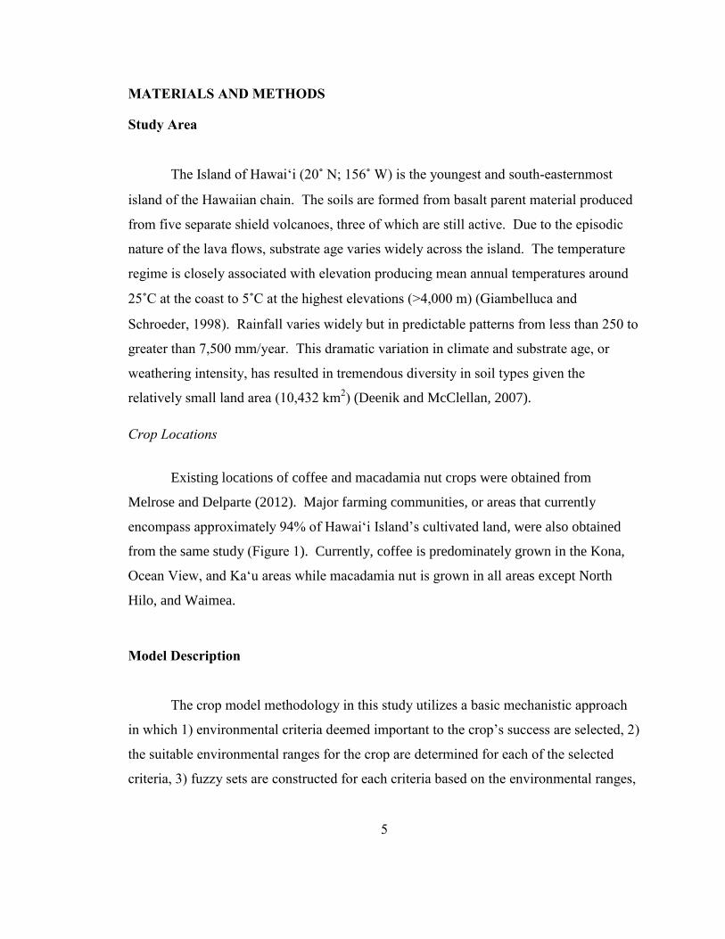
The Island of Hawai‘i (20˚ N; 156˚ W) is the youngest and south-easternmost

island of the Hawaiian chain. The soils are formed from basalt parent material produced

from five separate shield volcanoes, three of which are still active. Due to the episodic

nature of the lava flows, substrate age varies widely across the island. The temperature

regime is closely associated with elevation producing mean annual temperatures around

25˚C at the coast to 5˚C at the highest elevations (>4,000 m) (Giambelluca and

Schroeder, 1998). Rainfall varies widely but in predictable patterns from less than 250 to

greater than 7,500 mm/year. This dramatic variation in climate and substrate age, or

weathering intensity, has resulted in tremendous diversity in soil types given the

relatively small land area (10,432 km2) (Deenik and McClellan, 2007).

Crop Locations

Existing locations of coffee and macadamia nut crops were obtained from

Melrose and Delparte (2012). Major farming communities, or areas that currently

encompass approximately 94% of Hawai‘i Island’s cultivated land, were also obtained

from the same study (Figure 1). Currently, coffee is predominately grown in the Kona,

Ocean View, and Ka‘u areas while macadamia nut is grown in all areas except North

Hilo, and Waimea.

Model Description

The crop model methodology in this study utilizes a basic mechanistic approach

in which 1) environmental criteria deemed important to the crop’s success are selected, 2)

the suitable environmental ranges for the crop are determined for each of the selected

criteria, 3) fuzzy sets are constructed for each criteria based on the environmental ranges,

6

representing the approximate niche of the crop, and 4) a crop suitability score is

calculated based on how closely the current or future environmental conditions match the

constructed fuzzy sets.

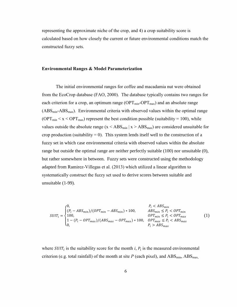
Environmental Ranges & Model Parameterization

The initial environmental ranges for coffee and macadamia nut were obtained

from the EcoCrop database (FAO, 2000). The database typically contains two ranges for

each criterion for a crop, an optimum range (OPTmin-OPTmax) and an absolute range

(ABSmin-ABSmax). Environmental criteria with observed values within the optimal range

(OPTmin < x < OPTmax) represent the best condition possible (suitability = 100), while

values outside the absolute range (x < ABSmin | x > ABSmax) are considered unsuitable for

crop production (suitability = 0). This system lends itself well to the construction of a

fuzzy set in which case environmental criteria with observed values within the absolute

range but outside the optimal range are neither perfectly suitable (100) nor unsuitable (0),

but rather somewhere in between. Fuzzy sets were constructed using the methodology

adapted from Ramirez-Villegas et al. (2013) which utilized a linear algorithm to

systematically construct the fuzzy set used to derive scores between suitable and

unsuitable (1-99).

{

(1)

where is the suitability score for the month i, is the measured environmental

criterion (e.g. total rainfall) of the month at site P (each pixel), and ABSmin, ABSmax,

7

OPTmin, and OPTmax are the absolute and optimal environmental ranges for the criterion

of a particular crop.

Each criterion’s suitability score (CSUIT) was calculated on a per pixel basis as the

average score of all months in a crop’s growing season

∑

(2)

where m is the number of months in a growing season. Time is summarized on an

average annual basis, therefore the growing season for coffee and macadamia nut is

twelve months. Using equation 2 incorporates the monthly distribution of environmental

suitability scores into the evaluation process.

Six environmental criteria were selected to evaluate coffee and macadamia nut

crop suitability. These criteria were rainfall (mean monthly/annual total), temperature

(mean minimum and maximum monthly), depth to restrictive layer, soil drainage, pH,

and slope. All criteria were evaluated using the equations above with the following

variations: (1) because the temperature criterion was evaluated using two datasets (i.e.

maximum and minimum mean monthly temperatures), both datasets were evaluated

separately for each site (P) and the minimum suitability score was selected as the

value for temperature; (2) when evaluating rainfall suitability for coffee, annual rainfall

was used as opposed to monthly rainfall because even monthly distribution of rainfall is

not necessarily advantageous for coffee bean production (Bittenbender and Smith, 2008);

(3) depth to restrictive layer did not require evaluation of maximum parameters (ABSmax,

OPTmax) and slope did not require evaluation of minimum parameters (ABSmin, OPTmin);

and (4) one suitability score, as opposed to monthly scores, was calculated for soil

properties (drainage class, depth, pH, and slope) which were assumed to be constant

throughout the duration of the study.

8

The overall suitability score for each crop was calculated on a per pixel basis

using a “Fuzzy And” overlay of all criteria, which returns the minimum value of the sets

the cell location belongs to

(3)

where n is the number of criteria used in the evaluation. This conservative approach is

useful for setting baseline thresholds for criteria (e.g. all criteria must have at least 50%

suitability). Additionally, this approach is also well suited to crop growth applications in

which the law of the minimum is often referenced (Paris, 1992). The law of the

minimum states that crop yield is proportional to the amount of the most limiting

nutrient. While nutrient levels are not evaluated in this study, the same idea can be

applied to environmental conditions and has been utilized in similar GIS crop-suitability

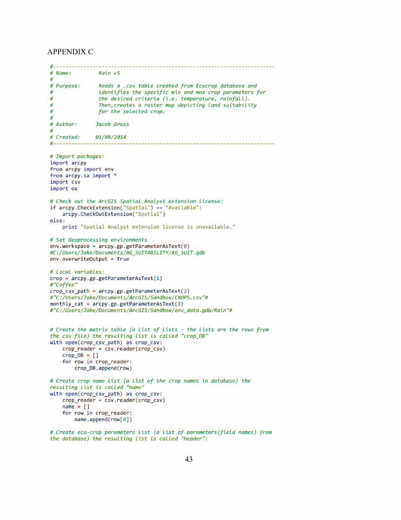
analysis (Bowen and Hollinger, 2002). All calculations were performed within ESRI

ArcMap 10.1 using python scripting. The modular design was utilized so that each

environmental criterion was evaluated separately producing individual suitability maps,

then all maps were combined into a final overall suitability map. This approach allows

flexibility within the model and the ability to add new evaluation criteria with minimal

changes to the python scripting (See Appendix B and C for additional information on the

structure of the model and an example of the python script).

Data Collection and Processing

Environmental Criteria

Datasets depicting current conditions for the six environmental criteria were

obtained from various sources. Mean monthly rainfall for the Island of Hawai’i was

obtained from the Rainfall Atlas of Hawai’i (Giambelluca et al., 2013). These values

9

originated from a 30-year base period (1978-2007) and were summarized as 8.1-

arcsecond spatial units (approximately 234 x 250 m in Hawai’i). The temperature dataset

was obtained from the PRISM Climate Group (Daly and Halbleib, 2006). Data included

average interpolated minimum and maximum monthly temperature surfaces from 1971-

2000. Original resolution is in 15-arc second spatial units (approximately 500 m in

Hawai’i).

Spatial and tabular data of soil properties (depth, drainage, and pH) were obtained

from the USDA-NRCS Web Soil Survey (Soil Survey Staff, 2014). The soil survey uses

vector-based polygons as its spatial unit, referred to as map units. Each map unit

contains tabular data of one or more soil types, or components, found within the area

along with its estimated proportional contribution to the map unit. The NRCS Soil Data

Viewer 6.1 (USDA, 2011) was used to aggregate and summarize soil properties from the

soil horizon and component level to the map unit level. Depth and pH were aggregated

by a weighted average algorithm while drainage class was aggregated using a dominant

condition algorithm, both algorithms were provided within the Soil Data Viewer

application. Estimates of slope were derived from USGS 7.5-minute digital elevation

model (DEM) quads for the Hawaiian Islands (DOC, 2007). All datasets were

transformed onto a 100 m Universal Transverse Mercator (UTM) projection using the

1983 North American Datum (NAD83).

Future Environmental Conditions

Future estimations of temperature and rainfall were determined by the Hawai’i

regional climate model (HRCM) (Lauer et al., 2013; Zhang et al., 2012). The HRCM is a

nested version of the Weather Research and Forecasting (WRF) model V3.3 that

produces high resolution cover over the Hawaiian Islands through forced lateral boundary

conditions. Currently the HRCM provides 3 km horizontal resolution across all the main

Hawaiian Islands. HRCM produces daily projections of rainfall and temperature over a

20-year period for both “present day” (1990-2009) and the late 21st century (2080-2099).

10

On a per pixel basis, daily projections of temperature and rainfall from the HRCM

were summarized into three variables (monthly [or annual] total rainfall, maximum

monthly temperature, and minimum monthly temperature) and then averaged across the

20-year period for both present and future conditions. The difference between present

and future conditions was calculated for each of the three variables for each month.

Finally, these differences were applied to their respective present climate datasets.

Data Accuracy and Analysis

Existing locations of coffee and macadamia nut crops were used to estimate the

accuracy of the crop model. Omission rate (OR) and root mean square error (RMSE)

were calculated to compare accuracy between 1) model results based solely on

environmental ranges referenced in the EcoCrop database and 2) environmental ranges

adjusted to reflect values referenced specifically for Hawai‘i .

(4)

√∑

(5)

where n is the total number of pixels representing the existing locations of coffee or

macadamia nut, X is the corresponding suitability value of the pixel divided by 100, and

nsuit is the number of pixels with suitability scores greater than zero. While lower scores

indicate increased accuracy of the model for both measurements, a RMSE value of zero

is unlikely because actual farmland may have been modified to increase crop suitability

and this modification would not have been captured within the environmental datasets.

Additionally, histograms of suitability scores for areas where crops are currently grown

were created to indicate producer’s accuracy at increasing thresholds of suitability level.

11

Change in crop suitability score was calculated on a per pixel basis as the

difference between future and current suitability scores. Zonal statistics were used to

summarize the mean difference in suitability scores at major farming communities and

current crop locations across Hawai’i Island. Land that was not identified as zoned for

agriculture according to the Hawai‘i Land Use Commission’s State Land Use District

Boundaries (Hawaii, 2013) was removed from consideration in the analysis. Finally, a

map of relative change in suitability score was created for locations with current and

future suitability scores above 50 for use in land management decision making.

12

RESULTS

Crop Parameters & Current Crop Suitability

The environmental ranges for coffee and macadamia nut used to parameterize the

crop suitability model were obtained from two main sources: FAO’s EcoCrop (2000)

database and local sources from Hawai‘i (Table 1). Local sources included published

literature and expert knowledge on crop requirements and were used to update the

EcoCrop parameters for the specific conditions encountered in Hawai‘i. Specifically, the

optimal and absolute ranges for soil depth were reduced substantially to prevent

excluding the almost pure lava soil conditions in Kona and elsewhere of which is

surprisingly accommodating to coffee and macadamia nut orchards. Absolute ranges for

drainage class were altered because the EcoCrop parameters only utilized three drainage

classes while the Hawai‘i Soil Survey includes seven drainage classes. Slope

requirements were not available in the EcoCrop database. However, steep terrain is a

common physical limitation to cultivation in Hawai‘i and therefore included as one of the

evaluation criteria. Local sources indicated that macadamia nut can occur in regions with

annual rainfall reaching 5080 mm/y in Hawai‘i as opposed to the absolute maximum of

3500 mm/y reported in Ecocrop.

All locations that can support coffee or macadamia production are not necessarily

producing these crops. Therefore, a comprehensive accuracy assessment of the crop

suitability maps (i.e. confusion matrix), as is typically performed with image

classification, is not possible. However, an estimate of producer’s accuracy (100% -

omission rate) can be calculated using existing crop locations. In this study the

producer’s accuracy refers to the proportion of pixels currently producing the crop that

were identified as “suitable” by the model. Before producer’s accuracy can be

determined, a choice must be made as to what score actually constitutes “suitable”. Table

2 shows the omission rate (OR) for the two parameterization sources (“Ecocrop” and

“Ecocrop + local sources”) when any score greater than zero is considered “suitable”.

Depending on the use of the model, a more restrictive (i.e. higher threshold) score may be

13

desired. Figure 2 shows the distribution of suitability scores at locations where the

respective crops are currently grown along with the producer’s accuracy when a

particular threshold score is used. For example, the coffee map will have a producer’s

accuracy of 83% if scores of 50 or higher are considered “suitable.” Comparatively,

macadamia shows a producer’s accuracy of 74% when using the same threshold score.

Root mean square error (RMSE) provides another measurement of accuracy

without the requirement of setting a binary threshold suitability score. However, a choice

must be made as to what the true suitability score is at locations where coffee or

macadamia nut is grown. This paper used “1” (suitability score of 100%) as the true

suitability score at locations where the respective crop is currently grown. This is a

conservative RMSE estimate because current crop locations have improved suboptimal

environmental conditions (e.g. irrigation) or may occur in suboptimal locations that

produce suboptimal yields. Nevertheless the accuracy calculations do provide a way in

which to compare model results when using Ecocrop parameters alone and results when

parameters are adjusted using local sources. Adjustments to the coffee and macadamia

environmental ranges based on local sources substantially improved the RMSE (84% and

73% change, respectively) and OR (96% and > 96% change, respectively) (Table 2).

Figure 3 shows the current distribution of crop suitability scores across Hawai‘i

Island. High coffee suitability scores are largely concentrated in farming communities

that currently grow coffee: Kona, Ocean View, and Ka‘u (Figure 3a). Additionally,

North Kohala, Hāmākua, and Pāhoa also show areas of high coffee suitability but

currently do not produce coffee on any sizeable scale. Low coffee suitability scores are

observable at upland portions of North Hilo, South Hilo, and Kea‘au largely due to

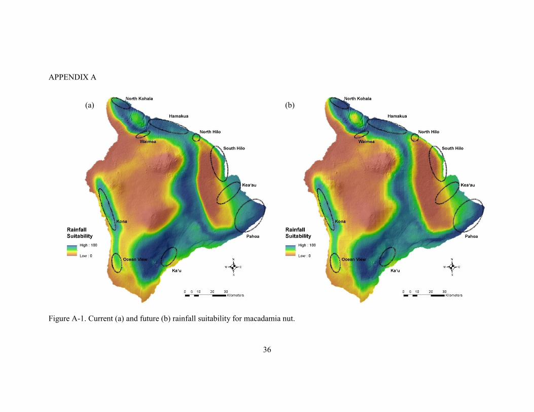
rainfall above optimum levels (see appendix A-1). Current macadamia suitability scores

show high suitability at all major farming communities, including the coastal portions of

North Hilo, South Hilo, and Kea‘au (Figure 3b).

14

Future Crop Suitability

Changes in the spatial distribution of suitability scores are varied and

concentrated in specific areas rather than evenly spread across the island (Figure 4a &

Figure 5a). The majority of area within each major farming community is projected to

encounter increased temperatures and increased annual rainfall. The only exception is

Ocean View which is expected to see decreased annual rainfall.

While the macadamia tree tolerates a wider range of temperature and rainfall

conditions than coffee, optimal nut production is referenced to favor slightly lower

temperatures than optimal coffee production. These slightly lower optimal growing

temperatures resulted in more noticeable declines in future temperature suitability for

macadamia as compared to coffee (Figure 4b & Figure 5b).

Fields where coffee is currently grown show little change in rainfall suitability (1

± 3 [mean ± one standard deviation]) and a small, variable decrease in temperature

suitability (-6 ± 9) (Figure 4b), most likely affecting only the farmland in the lowest

elevations. Average change in overall suitability score for coffee crop locations is

effectively zero (0 ± 3) (Figure 6a). Fields where macadamia is currently grown show

greater declines in rainfall (-4 ± 9), temperature (-20 ± 6), and overall (-7 ± 9) suitability

scores as compared with coffee.

The largest average declines in temperature suitability scores are observed in the

relatively low elevation farming communities of Pāhoa (coffee [COF] -16 ± 8;

macadamia [MAC] -22 ± 4) and Kea‘au (COF -14 ± 12; MAC -19 ± 9). Conversely, the

elevated farmland of Waimea shows overall positive changes in temperature suitability

(COF 37 ± 6; MAC 21 ± 5). The largest positive change in mean rainfall suitability score

occurred at Ka‘u (COF 10 ± 19; MAC 4 ± 6) and North Kohala (COF 4 ± 10; MAC 7 ±

5); however, the high standard deviation indicates changes in rainfall suitability were

variable across these locations.

15

The most conspicuous decrease in suitability scores for coffee and macadamia

occurs on the windward side, in a ring surrounding the wettest region of the island which

currently receives rainfall at or above the absolute maximum (ABSmax) threshold (Figure

5a, 6a, & Figure 7). Because rainfall is projected to increase throughout the windward

side of the Island, the unsuitable conditions will correspondingly expand.

Figure 7 shows a binary map of suitable and unsuitable locations using a

threshold suitability score of 50 (suitable ≥ 50, unsuitable < 50). Locations that

maintained suitability scores above 50 during current and future conditions are displayed

along with locations that changed from suitable to unsuitable and vice versa. Even with

predominate negative changes to temperature suitability; a substantial portion of land

with suitability scores above 50 remains available under future conditions.

16

DISCUSSION

Current Crop Suitability

Current suitability maps for coffee and macadamia nut show related spatial

distribution of suitability scores (Figure 3). Overlap in ranges is expected as these crops

share very similar environmental ranges and sometimes are even inter-planted. In

general, more locations appear suited for macadamia as compared with coffee. This

agrees with Hamilton and Fukunaga (1959), who stated that the climatic requirements for

growing macadamias are not as strict as those of coffee and therefore macadamias should

grow both above and below the coffee belt in Kona. While still highly suitable,

macadamia shows slightly lower scores than coffee within the Kona area. This is due in

part to uneven seasonal distribution of rainfall. In the Kona area, suitability scores for

macadamia are slightly penalized for the drier winter months. Conversely, the dry

winter months are actually beneficial to coffee production, so evaluation of rainfall

distribution was removed from coffee suitability analysis. This was achieved by utilizing

annual rainfall in place of monthly rainfall.

Future Crop Suitability

The deviation around the mean change in temperature and rainfall suitability

scores indicates that even these community level delineations may be too expansive to

adequately summarize future climate suitability on Hawai‘i Island. This reinforces the

idea that mitigation strategies will need to be site specific.

Locations on the upper windward slopes of Mauna Kea and Mauna Loa, result in

some of the largest positive changes in total suitability for macadamia and coffee (Figure

4a & Figure 5a). These areas witness both increased temperature and rainfall suitability.

A large portion of the land is located in non-agricultural zones or areas with limited

accessibility, away from currently existing farming communities and associated

infrastructure. However, the area between the Hamakua and Waimea farming

communities may provide some potential for coffee or macadamia nut crops to follow

17

suitable environmental conditions in the future and remain near areas of high agricultural

activity.

The Kona farming community appears suited to maintain coffee and macadamia

production in the future (Figure 6 & 7). If anything, effort could be made to discourage

additional plantings in the lowest elevations within the community to avoid potential

negative effects from temperature increases. Ka‘u also appears to be able to maintain

production, and may even see positive impacts on future coffee production. Areas like

Pāhoa and Kea‘au have limited strategies due to the lack of elevation in the area. Plus,

projections of increased heavy rainfall will encroach from the highlands further reducing

the locations available. If coffee production is desired in these areas, growers could try

experimenting with shaded coffee in the relatively more suitable coastal areas. Shaded

coffee has been found to help reduce temperatures in other coffee growing areas outside

of Hawai‘i. Finally, locations like South Hilo may have to abandon coffee and

macadamia production if increased rainfall does become a problem. Because macadamia

farms here are already in areas with rainfall above optimal levels and they are situated

along increasing rainfall gradients, South Hilo provides an opportunity to research and

better understand the upper limits of rainfall for production.

In this study, the absolute maximum rainfall threshold for macadamia was

substantially increased compared to the value reported in the Ecocrop database (Table 1).

It might be assumed that this discrepancy in upper rainfall limits is a result of

“excessively-drained” lava lands on Hawai‘i Island which might lessen any potential

waterlogging issues. However, the USDA soil survey for Hawai‘i indicates that a

majority of the macadamia farms are found on “well-drained” soils as opposed to

“excessively-drained” soils. Additionally, farms occurring on “excessively-drained” soils

actually receive less rainfall than the “well-drained” soils.

Because the absolute maximum threshold is based on crop occurrence, there is

some uncertainty whether or not this value is indeed the maximum amount tolerable for

macadamia or just the maximum amount currently observed. Still, it is generally

18

accepted that high levels of rainfall can reduce optimal production in Hawai‘i. In 2006,

the Hawai‘i Macadamia Nut Association (HMCA) reported a three-year trend of

declining yields at farms near Hilo reportedly due to excessive rainfall (Rietow, 2006).

Negative impacts of high rainfall in macadamia production can include direct effects such

as losses from floods and poor pollination/nut set (Yamaguchi, 2005) to indirect effects

like trees allocating resources towards developing wood at the expense of flowers and

nuts, or increased risk of fungal diseases (Bittenbender and Hirae, 1990). Macadamia

nuts also must be harvested more frequently in high rainfall areas to prevent mold and

fungal growth on the nuts, which increases labor costs.

Coffee production can also be negatively impacted by increased rainfall,

particularly if excessive rainfall occurs during flowering and harvest periods

(Bittenbender and Smith, 2008). Surprisingly, upper thresholds in rainfall are very rarely

mentioned in growing guides for coffee and macadamia. The projections from the

Hawai‘i regional climate model along with the results of this study highlight the

importance of determining reliable estimates on the upper rainfall limits to coffee and

macadamia production, particularly for the use in future site selection and agricultural

planning.

19

Model Accuracy

Producer’s accuracy is a common measurement of accuracy in image

classification. Producer’s accuracy represents the fraction of correctly classified pixels

with regard to all pixels of the ground truth class. In this study, locations currently

cultivating coffee or macadamia represent the respective ground truth classes.

Calculations of RMSE and OR indicate that producer’s accuracy was improved when

environmental ranges from local sources were used as the model parameters (Table 2).

Histograms of suitability scores at currently cultivated sites (Figure 2) show a majority of

the scores occurring at or above 70 and 60 for coffee and macadamia, respectively.

These histograms can also be used to select the desired producer’s accuracy threshold if a

binary map of suitable (1) and unsuitable (0) sites is desired.

Model Formulation

Because the evaluation procedure used to calculate suitability scores is based on

average conditions, anomalous months or years are not specifically considered.

Additionally, phenomena occurring at temporal scales less than one month (i.e. three

week drought or torrential rainfall) are not well represented by this approach. Recent

studies suggest increased risk of widespread heavy rain events in Hawai‘i is low (Timm

et al., 2013) with higher summer precipitation and lower winter precipitation (Timm and

Diaz, 2009). However, increased droughts are expected to occur in areas that are already

dry (Timm et al., 2013).

Unfortunately, this study was unable to provide an indication of the relationship

between suitability and yield. This is because 1) widespread yield data are largely

unavailable and 2) yield data would need to be corrected based on the wide variety of

planting, growing, and harvesting techniques used by each individual farmer.

While suitability scores cannot be used as direct predictions of yield, this

modeling approach still provides a number of advantages. First of all, using fuzzy sets to

model a crop’s environmental range provides an intuitive parameterization method

20

because farming resources frequently use optimal ranges when describing a crop’s

physiology. Additionally, using fuzzy sets to rate each criterion’s suitability rather than

binary or categorical suitability rating helps reduce mapping errors caused by inaccuracy,

imprecision, and ambiguity in the datasets. At the community scale, this methodology

can also provide a useful application in understanding a crop’s current climate suitability

and distribution. For example, if the model shows a location to be suitable, but the crop

is not actually cultivated there, additional data can be explored to determine what is

actually limiting production in the area. On the other hand, cultivated sites that are not

considered suitable can be explored further to determine what factors are responsible for

the successful crop. This approach allows environmental ranges, environmental datasets,

and future climate projections to be easily modified to accommodate new knowledge and

data availability. Therefore, the procedure can be applied to a wide range of crop types

which will be useful for evaluating Hawai‘i’s diversified agricultural system.

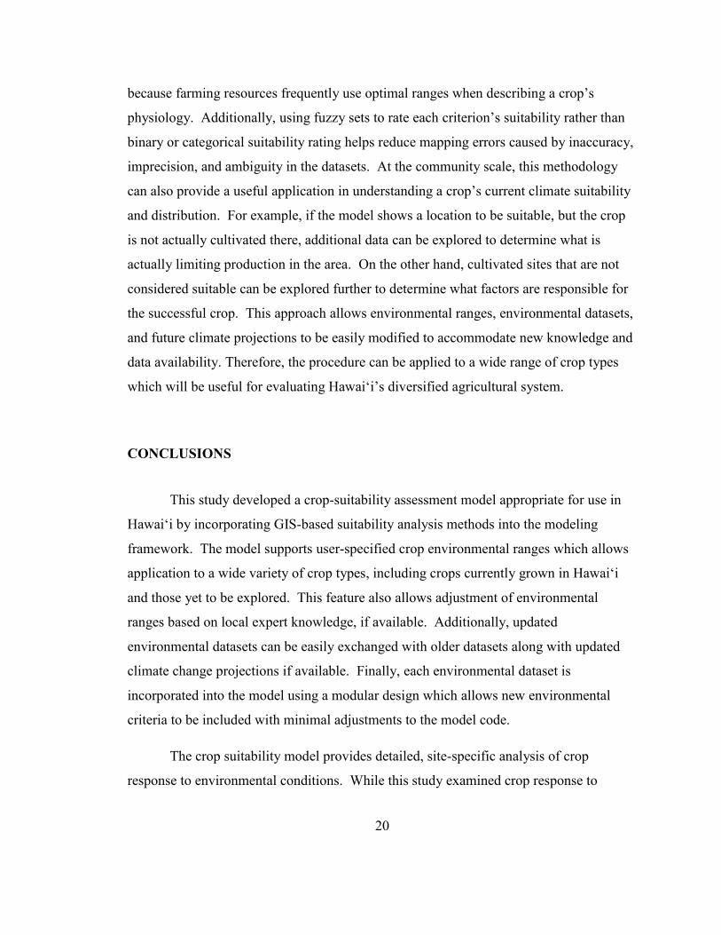
CONCLUSIONS

This study developed a crop-suitability assessment model appropriate for use in

Hawai‘i by incorporating GIS-based suitability analysis methods into the modeling

framework. The model supports user-specified crop environmental ranges which allows

application to a wide variety of crop types, including crops currently grown in Hawai‘i

and those yet to be explored. This feature also allows adjustment of environmental

ranges based on local expert knowledge, if available. Additionally, updated

environmental datasets can be easily exchanged with older datasets along with updated

climate change projections if available. Finally, each environmental dataset is

incorporated into the model using a modular design which allows new environmental

criteria to be included with minimal adjustments to the model code.

The crop suitability model provides detailed, site-specific analysis of crop

response to environmental conditions. While this study examined crop response to

21

climate change, many other applications are possible ranging from farm specific

problems like determining what crop is most suitability in a specific area or, when the

best time of year is to plant a particular annual crop; to state-wide problems like

determining appropriate sites for public agricultural facilities.

This paper utilized coffee and macadamia as a case study for determining crop

response to climate change on Hawai‘i Island. The key findings for coffee and

macadamia production on the Island of Hawai‘i are as follows:

Future rainfall and temperature projections support continued coffee production in

the major coffee producing areas on Hawai‘i Island.

Locations currently cultivating macadamia are predicted to encounter declines in

future production due to above optimal temperatures at low elevation farms and

above optimal rainfall at upper elevation farms, particularly on the windward side

of the Island.

Mean temperature suitability for coffee and macadamia is projected to decline for

most major farming communities. However, future temperature suitability is still

predicted to remain above 50% over the next 80 years within farming

communities.

Upper rainfall levels will be an important factor influencing the continued

production of macadamia nut at windward farming communities. Additional

research on upper rainfall thresholds for macadamia production will be beneficial

to future site selection of orchards.

Continued coffee and macadamia production on Hawai‘i Island will require

community specific strategies because each farming community will encounter

different challenges and opportunities in crop production related to the current

and future distribution of rainfall and temperature.

22

TABLES

Table 1. Optimum (OPT) and absolute (ABS) environmental ranges for coffee and macadamia nut used in the analyses.

The “EcoCrop” source includes only the environmental ranges found within the FAO’s EcoCrop Database. The “+Local

Sources” shows adjustments made to environmental ranges based on local sources including reports and expert opinion.

Temperature (˚C)

Rainfall (mm/y)

Drainage (class)

Depth (cm)

Soil pH

Slope (%)

Coffee OPT ABS OPT ABS OPT ABS OPT ABS

OPT ABS

OPT ABS

Source:

EcoCrop 14-28 10-34

1400-2300

750-4200

well well

>150 50-150

5.5-7.0

4.3-8.4

NA NA

+Local Sources

well poor-excess

>17a 1-17a

5.5c-7.0b

3.0-9.0

<28b <38

Macadamia nut

Source:

EcoCrop 10-26 8-35

1000-3000

700-3500

well well

50-150

50-150

5.0-6.0

4.5-7.0

NA NA

+Local Sources 14d-26

1524e-3048e

510d-5080f

well poor-excess

>17a 1-17a

5.0c-6.5c

3.0-9.0

<20f <30

a H.C. Bittenbender, personal communication (Feb 18th, 2014)

b Bittenbender and Smith (2008)

c Uchida and Hue (2000)

d Nagao and Hirae (1992) e

Hawaii (1987) f Shigeura and Ooka (1984)

23

Table 2. Root mean square error (RMSE) and omission rate (OR)

for crop model using EcoCrop parameters alone and EcoCrop

parameters plus adjustments according to local sources. Percent

change in RMSE and OR when local sources are added are shown

in parentheses.

Coffee

RMSE

OR

Source:

EcoCrop

0.69

0.25

+Local Sources

0.11 (84%)

0.01 (96%)

Macadamia nut

Source:

EcoCrop

0.63

0.20

+Local Sources

0.17 (73%)

<0.01 (>96%)

24

FIGURES

Figure 1. Areas of crop cultivation (in red) and major farming communities on Hawai‘i

Island, as in Melrose and Delparte (2012). Areas are named according to districts or

closest major towns: North Kohala, Waimea, Hāmākua, North Hilo, South Hilo, Kea‘au,

Pāhoa, Ka‘u, Ocean View, and Kona.

25

Figure 2. Histograms of (a) coffee suitability scores and (b) macadamia nut suitability

scores at locations where the respective crop is currently cultivated. Percentages across

the top indicate the proportion of actual farm locations captured if the corresponding

suitability score is chosen as the binary threshold between suitable (1) and unsuitable (0).

26

Figure 3. Coffee (a) and macadamia nut (b) crop suitability under current environmental conditions. Core crop lands and major roads

are included for reference. A gray mask is used to exclude land that was not identified as zoned for agriculture according to the

Hawai‘i Land Use Commission’s State Land Use District Boundaries (Hawaii, 2013)

(a) (b)

27

Figure 4. (a) Change in coffee crop suitability scores across Hawai‘i Island. (b) Changes

in temperature and rainfall suitability scores for each major farming community (error

bars represent one standard deviation).

28

Figure 5. (a) Change in macadamia crop suitability scores across Hawai‘i Island. (b)

Changes in temperature and rainfall suitability scores for each major farming community

(error bars represent one standard deviation).

29

Figure 6. Mean change in suitability scores (temperature, rainfall, and overall suitability)

at current farming locations and major farming communities for (a) coffee and (b)

macadamia nut (tails represent one standard deviation from mean overall change).

0

-12 -10 -6

-11 -7

15

-1 1 0

6

-30

-20

-10

0

10

20

30

40

Me

an Δ

in S

uit

abili

ty S

core

Overall Temperature Rainfall

-7 -8

-14 -11

-14

-6

4

-6 -2 -1 0

-30

-20

-10

0

10

20

30

40

Me

an Δ

in S

uit

abili

ty S

core

Overall Temperature Rainfall

A

B

30

Figure 7. Binary suitability maps for coffee (a) and macadamia (b) using a cutoff suitability score of 50. Locations that maintain

suitability scores above 50 are shown in brown, locations projected to increase in suitability above 50 are shown in green, locations

projected to decrease below 50 due to changes in temperature or rainfall suitability are shown in red.

(a) (b)

31

REFERENCES

Abercrombie, N., 2010. A New Day in Hawaii. State of Hawaii.

Bittenbender, H. and Smith, V.E., 2008. Growing Coffee in Hawaii.

Bittenbender, H.C. and Hirae, H.H., 1990. Common problems of macadamia nut in

Hawaii.

Bowen, R.C. and Hollinger, S.E., 2002. Alternative Crops Web Site, Illinois State Water

Survey. Champaign Illinois, http://www.sws.uiuc.edu/data/altcrops/.

Brown, M. and Funk, C., 2008. Climate: Food security under climate change. Science,

319: 580-581.

Burrough, P.A. and McDonnell, R., 1998. Principles of geographical information

systems, 333. Oxford university press Oxford.

Challinor, A., Wheeler, T., Craufurd, P. and Slingo, J., 2005. Simulation of the impact of

high temperature stress on annual crop yields. Agricultural and Forest Meteorology,

135(1): 180-189.

Challinor, A.J., Ewert, F., Arnold, S., Simelton, E. and Fraser, E., 2009. Crops and

climate change: progress, trends, and challenges in simulating impacts and informing

adaptation. Journal of Experimental Botany, 60(10): 2775-2789.

Collins, M., Steiner, F. and Rushman, M.J., 2001. Land-use suitability analysis in the

United States: historical development and promising technological achievements.

Environmental Management, 28(5): 611-621.

Daly, C. and Halbleib, M., 2006. Pacific Islands Average Monthly or Annual

Precipitation, 1971-2000 Normals. In: PRISM Climate Group (Editor). Available online:

http://prism.oregonstate.edu, Oregon State University: Corvallis, OR, USA.

Deenik, J. and McClellan, A.T., 2007. Soils of Hawai'i, University of Hawai'i at Manoa,

Cooperative Extension Service, College of Tropical Agriculture and Human Resources.

Dingeman, R., 2011. Local Food Market Demand Study of Oahu Shoppers, OmniTrak

Group Inc., Ulupono Initiative.

DOC, 2007. Digital Elevation Models (DEMs) for the main 8 Hawaiian Islands.

Department of Commerce (DOC), National Oceanic and Atmospheric Administration

(NOAA), Silver Spring, MD.

32

FAO, Food and Agriculture Organization of the United Nations, 2000. The Ecocrop

Database, Rome, Italy.

Fowler, H., Blenkinsop, S. and Tebaldi, C., 2007. Linking climate change modelling to

impacts studies: recent advances in downscaling techniques for hydrological modelling.

International Journal of Climatology, 27(12): 1547-1578.

Giambelluca, T.W. and Schroeder, T.A., 1998. Climate. In: S.P. Juvik and J.O. Juvik

(Editors), Atlas of Hawaii University of Hawaii Press, Honolulu, HI, pp. 49-59.

Gregory, P.J., Ingram, J.S. and Brklacich, M., 2005. Climate change and food security.

Philosophical Transactions of the Royal Society B: Biological Sciences, 360(1463):

2139-2148.

Hamilton, R.A. and Fukunaga, E.T., 1959. Growing Macadamia Nuts in Hawaii, Hawaii

Agricultural Experiment Station.

Hawaii, Department of Agriculture, 2005. Incentives For Important Agriculutural Lands,

Act 183, SLH.

Hawaii, Office of Planning, 2013. State Land Use District Boundaries.

Hawaii, State of, 1987. Macadamia Industry Analysis Number 4. Agricultural Industry

Analysis: The Status, Potential, and Problems of Hawaiian Crops. College of Tropical

Agriculture and Human Resources,University of Hawaii at Manoa, Honolulu, HI, 101 pp.

Hawaii, State of, 2008. Hawaii 2050 Sustainability Plan: Charting a Course for Hawaii's

Sustainable Future, Sustainability Task Force, Honolulu, HI.

Hawaii, State of, 2012. Increased Food Security and Self-Sufficiency Strategy, Office of

Planning, Department of Business Economic Development & Tourism, Honolulu, HI.

IPCC, 2007. Fourth Assessment Report: Climate Change 2007 (AR4), IPCC, Geneva,

Switzerland.

Lane, A. and Jarvis, A., 2007. Changes in climate will modify the geography of crop

suitability: agricultural biodiversity can help with adaptation. Journal of Semi-arid

Tropical Agricultural Research, 4(1): 1-12.

Lauer, A., Zhang, C., Elison-Timm, O., Wang, Y. and Hamilton, K., 2013. Downscaling

of Climate Change in the Hawaii Region Using CMIP5 Results: On the Choice of the

Forcing Fields*. Journal of Climate, 26(24).

33

Leung, P. and Loke, M., 2008. The Contribution of Agriculture to Hawai'i's Economy:

2005, University of Hawai'i at Manoa, College of Tropical Agriculture and Human

Resources.

Lobell, D.B. et al., 2008. Prioritizing climate change adaptation needs for food security in

2030. Science, 319(5863): 607-610.

Lobell, D.B., Schlenker, W. and Costa-Roberts, J., 2011. Climate trends and global crop

production since 1980. Science, 333(6042): 616-620.

Loke, M.K. and Leung, P., 2013. Hawaiis food consumption and supply sources:

benchmark estimates and measurement issues. Agricultural and Food Economics, 1(1):

10.

Malczewski, J., 2004. GIS-based land-use suitability analysis: a critical overview.

Progress in Planning, 62(1): 3-65.

Mathur, P., Ramirez-Villegas, J. and Jarvis, A., 2012. The Impacts of Climate Change on

Tropical and Sub-tropical Horticultural Production. Tropical Fruit Tree Species and

Climate Change: 27.

Melrose, J. and Delparte, D., 2012. Hawai'i County Food Self-Sufficiency Baseline 2012,

University of Hawai'i at Hilo.

Nagao, M.A. and Hirae, H.H., 1992. Macadamia: Cultivation and physiology. Critical

reviews in plant sciences, 10(5): 441-470.

Nisar Ahamed, T., Gopal Rao, K. and Murthy, J., 2000. GIS-based fuzzy membership

model for crop-land suitability analysis. Agricultural Systems, 63(2): 75-95.

Paris, Q., 1992. The Return of von Liebig's “Law of the Minimum”. Agronomy Journal,

84(6): 1040-1046.

PIRCA, 2012. Climate Change and Pacific Islands: Indicators and Impacts, Pacific

Islands Regional Climate Assessment (PIRCA), Washington, DC: Island Press.

Ramirez-Villegas, J., Jarvis, A. and Laderach, P., 2013. Empirical approaches for

assessing impacts of climate change on agriculture: The EcoCrop model and a case study

with grain sorghum. Agricultural and Forest Meteorology, 170: 67-78.

Rietow, D., 2006. Presidents Report, Hawaii Macadamia Nut Association 46th Annual

Conference Proceedings, Keauhou, Hawaii.

34

Rivington, M. and Koo, J., 2011. Report on the meta-analysis of crop modelling for

climate change and food security survey, CGIAR Research Program on Climate Change,

Agriculture, and Food Security.

Shigeura, G.T. and Ooka, H., 1984. Macadamia Nuts in Hawaii: History and Production.

Soil Survey Staff, 2014. Web Soil Survey. Natural Resource Conservation Service, US

Department of Agriculture, Available online at: http://websoilsurvey.nrcs.usda.gov/.

Accessed: [9 June 2014].

Suryanata, K., 2002. Diversified Agriculture, Land Use, and Agrofood Networks in

Hawaii. Economic Geography, 78(1): 71-86.

Timm, O. and Diaz, H.F., 2009. Synoptic-statistical approach to regional downscaling of

IPCC twenty-first-century climate projections: seasonal rainfall over the Hawaiian

Islands. Journal of Climate, 22(16).

Timm, O., Takahashi, M., Giambelluca, T.W. and Diaz, H.F., 2013. On the relation

between large‐scale circulation pattern and heavy rain events over the Hawaiian Islands:

Recent trends and future changes. Journal of Geophysical Research: Atmospheres,

118(10): 4129-4141.

Uchida, R. and Hue, N.V., 2000. Soil Acidity and Liming. In: J.A. Silva and R. Uchida

(Editors), Plant Nutrient Management in Hawaii's Soils, Approaches for Tropical and

Subtropical Agriculture. College of Tropical Agriculture and Human Resources,

University of Hawaii at Manoa.

USDA, National Agricultural Statistics Service (NASS), 2013. Statistics of Hawaii

Agriculture.

USDA, Natural Resource Conservation Service, 2011. Soil Data Viewer 6.0 User Guide.

White, J.W., Hoogenboom, G., Kimball, B.A. and Wall, G.W., 2011. Methodologies for

simulating impacts of climate change on crop production. Field Crops Research, 124(3):

357-368.

Wilby, R.L. et al., 2009. A review of climate risk information for adaptation and

development planning. International Journal of Climatology, 29(9): 1193-1215.

Yamaguchi, A., 2005. Crop Models to Show Importance of Rainfall and Temperature on

Yield, Hawaii Macadamia Nut Association 45th Annual Conference Proceedings,

Keauhou, Hawaii.

Zadeh, L.A., 1965. Fuzzy sets. Information and control, 8(3): 338-353.

35

Zhang, C., Wang, Y., Lauer, A. and Hamilton, K., 2012. Configuration and Evaluation of

the WRF Model for the Study of Hawaiian Regional Climate. American Meteorological

Society, 140(10): 3259-3277.

36

APPENDIX A

Figure A-1. Current (a) and future (b) rainfall suitability for macadamia nut.

(a) (b)

37

Figure A-2. Current (a) and future (b) temperature suitability for macadamia.

(a) (b)

38

Figure A-3. Soil drainage suitability for coffee and macadamia.

39

Figure A-4. Soil depth suitability for coffee and macadamia

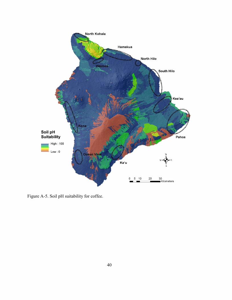
40

Figure A-5. Soil pH suitability for coffee.

41

Figure A-6. Slope suitability for macadamia.

42

APPENDIX B

Figure B-1. ArcMap Model Builder diagram depicting the modular structure of the crop

suitability model. Each environmental criterion utilizes a separate python script which produces a

corresponding suitability map. Blue ovals represent user supplied variables including rasters of

environmental datasets. The Depth, pH, Drainage, and Slope scripts accept single raster files,

while the Temperature script accepts raster catalogs (consisting of twelve rasters) of monthly

temperature values. The rainfall evaluation script accepts either a single raster with annual

rainfall values or a raster catalog with twelve, monthly rainfall rasters. The “crops.csv” is a

comma separated table consisting of environmental ranges for each criteria and each crop.

43

APPENDIX C

44

45