Remote Sensing of Environment 114 (2010) 2624–2636

Contents lists available at ScienceDirect

Remote Sensing of Environment

j ourna l homepage: www.e lsev ie r.com/ locate / rse

Landslide susceptibility mapping using downscaled AMSR-E soil moisture: A casestudy from Cleveland Corral, California, US

Ram L. Ray a,⁎, Jennifer M. Jacobs b, Michael H. Cosh c

a Department of Civil and Construction Engineering, San Diego State University, USAb Department of Civil Engineering, University of New Hampshire, 35 Colovos Rd. Durham, NH 03824, USAc USDA ARS, Hydrology and Remote Sensing Lab, Beltsville, MD 20705, USA

⁎ Corresponding author. 5500 Campanile Dr. San Dieg594 0929; fax: +1 619 594 8078.

E-mail address: ramlakhan37@gmail.com (R.L. Ray).

0034-4257/$ – see front matter © 2010 Elsevier Inc. Aldoi:10.1016/j.rse.2010.05.033

a b s t r a c t

a r t i c l e i n f o

Article history:Received 3 November 2009Received in revised form 28 April 2010Accepted 31 May 2010

Keywords:AMSR-ERemote sensingVIC-3LLandslideSoil moistureSlope stability

As soil moisture increases, slope stability decreases. Remotely sensed soil moisture data can provide routineupdates of slope conditions necessary for landslide predictions. For regional scale landslide investigations,only remote-sensing methods have the spatial and temporal resolution required to map hazard increases.Here, a dynamic physically-based slope stability model that requires soil moisture is applied using remote-sensing products from multiple Earth observing platforms. The resulting landslide susceptibility maps usingthe advanced microwave scanning radiometer (AMSR-E) surface soil moisture are compared to those createdusing variable infiltration capacity (VIC-3L) modeled soil moisture at Cleveland Corral landslide area inCalifornia, US. Despite snow cover influences on AMSR-E surface soil moisture estimates, a good relationshipbetween the downscaled AMSR-E's surface soil moisture and the VIC-3L modeled soil moisture is evident.The AMSR-E soil moisture mean (0.17 cm3/cm3) and standard deviation (0.02 cm3/cm3) are very close to themean (0.21 cm3/cm3) and standard deviation (0.09 cm3/cm3) estimated by VIC-3L model. Qualitative resultsshow that the location and extent of landslide prone regions are quite similar. Under the maximumsaturation scenario, 0.42% and 0.49% of the study area were highly susceptible using AMSR-E and VIC-3Lmodel soil moisture, respectively.

o, CA 92182, USA. Tel.: +1 619

l rights reserved.

© 2010 Elsevier Inc. All rights reserved.

1. Introduction

Remote-sensing and spatial analysis tools are widely used inlandslide studies including landslide detection, landslide assessment,natural hazard, landslide mapping, and landslide inventories (e.g.,Gorsevski et al., 2003; Guzzetti et al., 1999; Pradhan et al., 2006; vanWesten, 1994; Varnes, 1984). Remote-sensing data can be used topredict catastrophic events and hazardous areas (Ostir et al., 2003)and they have significant potential for landslide studies (Hong et al.,2007).

Landslide inventory maps can be developed by field surveying.However, surveying is time consuming, expensive and difficult forregional or global scales. On the other hand, landslide inventory mapscan be developed using aerial photography (Brarddinoni et al., 2003;Oka, 1998; van Westen & Getahun, 2003) as well as remotely senseddata with image analysis technique (Abdallah et al., 2007; Nichol &Wong, 2005). Over the past decade, the Earth Observing System (EOS)platforms have deployed a suite of instruments that monitor landconditions relevant to landslide hazard characterization such as LightDetection and Ranging (LiDAR), Interferometric Synthetic Aperture

Radar (InSAR), and Differential SAR Interferometry (DInSAR) data.The predominant use of remotely sensed data is to map landslidesafter they have occurred using aerial photographs (van Westen &Getahun, 2003), to characterize landslide distributions using aerialphotographs (Carrara et al., 1991), and to inventory landslides usingSPOT satellite images (Cheng et al., 2004). Multi-temporal satelliteimages are increasingly used to monitor, classify and detect landslides(Hervas et al., 2003; Mantovani et al., 1996).

For landslide analyses, Landsat™ and Advanced SpaceborneThermal Emission and Reflection Radiometer (ASTER) have beenused to derive land cover in regions including the Himalayas range(Saha et al., 2002; Sarkar & Kanungo, 2004; Zomer et al., 2002). InSARhas been used to locate and characterize landslides (e.g., Canuti et al.,2004; Singhroy & Molch, 2004). Kaab (2005) showed that recentShuttle Radar Topography Mission (SRTM) results are promising forcharacterizing topography in regions having landslides. Pelletier et al.(1997) indicated that continuous remote-sensing of soil moisturecoupled with a digital elevation model is a necessary component of asuccessful landslide hazard mitigation program. Their work recom-mended replacing soil moisture surrogates that have been usedextensively in slope stability analyses and landslide observations.Typically, slope stability is analyzed using wetness indices to estimatesoil wetness (Acharya et al., 2006; de Vleeschauwer & De Smedt,2002; Montgomery & Dietrich, 1994; van Westen & Trelirn, 1996). As

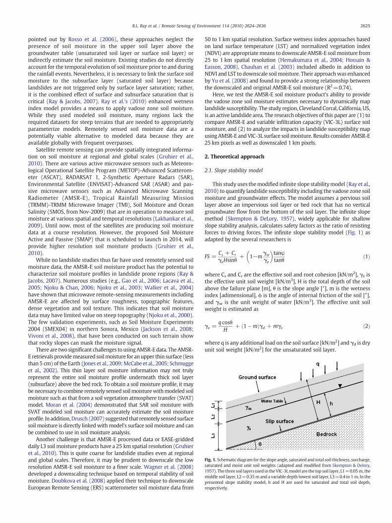
Fig. 1. Schematic diagram for the slope angle, saturated and total soil thickness, surcharge,saturated and moist unit soil weights (adapted and modified from Skempton & Delory,1957). The three soil layers used in theVIC-3Lmodel are the top soil layer, L1=0.05 m, themiddle soil layer, L2=0.35 m and a variable depth lowest soil layer, L3=0.4 to 1 m. In thepresented slope stability model, h and H are used for saturated and total soil depth,respectively.

2625R.L. Ray et al. / Remote Sensing of Environment 114 (2010) 2624–2636

pointed out by Rosso et al. (2006), these approaches neglect thepresence of soil moisture in the upper soil layer above thegroundwater table (unsaturated soil layer or surface soil layer) orindirectly estimate the soil moisture. Existing studies do not directlyaccount for the temporal evolution of soil moisture prior to and duringthe rainfall events. Nevertheless, it is necessary to link the surface soilmoisture to the subsurface layer (saturated soil layer) becauselandslides are not triggered only by surface layer saturation; rather,it is the combined effect of surface and subsurface saturation that iscritical (Ray & Jacobs, 2007). Ray et al.'s (2010) enhanced wetnessindex model provides a means to apply vadose zone soil moisture.While they used modeled soil moisture, many regions lack therequired datasets for steep terrains that are needed to appropriatelyparameterize models. Remotely sensed soil moisture data are apotentially viable alternative to modeled data because they areavailable globally with frequent overpasses.

Satellite remote sensing can provide spatially integrated informa-tion on soil moisture at regional and global scales (Gruhier et al.,2010). There are various active microwave sensors such as Meteoro-logical Operational Satellite Program (METOP)-Advanced Scatterom-eter (ASCAT), RADARSAT 1, 2-Synthetic Aperture Radars (SAR),Environmental Satellite (ENVISAT)-Advanced SAR (ASAR) and pas-sive microwave sensors such as Advanced Microwave ScanningRadiometer (AMSR-E), Tropical Rainfall Measuring Mission(TRMM)-TRMM Microwave Imager (TMI), Soil Moisture and OceanSalinity (SMOS, from Nov-2009) that are in operation to measure soilmoisture at various spatial and temporal resolutions (Lakhankar et al.,2009). Until now, most of the satellites are producing soil moisturedata at a course resolution. However, the proposed Soil MoistureActive and Passive (SMAP) that is scheduled to launch in 2014, willprovide higher resolution soil moisture products (Gruhier et al.,2010).

While no landslide studies thus far have used remotely sensed soilmoisture data, the AMSR-E soil moisture product has the potential tocharacterize soil moisture profiles in landslide prone regions (Ray &Jacobs, 2007). Numerous studies (e.g., Gao et al., 2006; Lacava et al.,2005; Njoku & Chan, 2006; Njoku et al., 2003; Walker et al., 2004)have shown that microwave remote-sensingmeasurements includingAMSR-E are affected by surface roughness, topographic features,dense vegetation and soil texture. This indicates that soil moisturedata may have limited value on steep topography (Njoku et al., 2000).The few validation experiments, such as Soil Moisture Experiments2004 (SMEX04) in northern Sonora, Mexico (Jackson et al., 2008;Vivoni et al., 2008), that have been conducted on such terrain showthat rocky slopes can mask the moisture signal.

There are two significant challenges to usingAMSR-E data. TheAMSR-E retrievals providemeasured soilmoisture for anupper thin surface (lessthan 5 cm) of the Earth (Jones et al., 2009;McCabe et al., 2005; Schmuggeet al., 2002). This thin layer soil moisture information may not trulyrepresent the entire soil moisture profile underneath thick soil layer(subsurface) above the bed rock. To obtain a soil moisture profile, it maybenecessary to combine remotely sensed soilmoisturewithmodeled soilmoisture such as that from a soil vegetation atmosphere transfer (SVAT)model. Moran et al. (2004) demonstrated that SAR soil moisture withSVAT modeled soil moisture can accurately estimate the soil moistureprofile. In addition,Drusch (2007) suggested that remotely sensedsurfacesoil moisture is directly linkedwithmodel's surface soil moisture and canbe combined to use in soil moisture analysis.

Another challenge is that AMSR-E processed data or EASE-griddeddaily L3 soil moisture products have a 25 km spatial resolution (Gruhieret al., 2010). This is quite coarse for landslide studies even at regionaland global scales. Therefore, it may be prudent to downscale the lowresolution AMSR-E soil moisture to a finer scale. Wagner et al. (2008)developed a downscaling technique based on temporal stability of soilmoisture. Doubkova et al. (2008) applied their technique to downscaleEuropean Remote Sensing (ERS) scatterometer soil moisture data from

50 to 1 km spatial resolution. Surface wetness index approaches basedon land surface temperature (LST) and normalized vegetation index(NDVI) are appropriatemeans to downscale AMSR-E soil moisture from25 to 1 km spatial resolution (Hemakumara et al., 2004; Hossain &Easson, 2008). Chauhan et al. (2003) included albedo in addition toNDVI and LST to downscale soil moisture. Their approachwas enhancedby Yu et al. (2008) and found to provide a strong relationship betweenthe downscaled and original AMSR-E soil moisture (R2=0.74).

Here, we test the AMSR-E soil moisture product's ability to providethe vadose zone soil moisture estimates necessary to dynamically maplandslide susceptibility. The study region, ClevelandCorral, California, US,is an active landslide area. The research objectives of this paper are (1) tocompare AMSR-E and variable infiltration capacity (VIC-3L) surface soilmoisture, and (2) to analyze the impacts in landslide susceptibility mapusing AMSR-E andVIC-3L surface soilmoisture. Results consider AMSR-E25 km pixels as well as downscaled 1 km pixels.

2. Theoretical approach

2.1. Slope stability model

This study uses themodified infinite slope stabilitymodel (Ray et al.,2010) to quantify landslide susceptibility including the vadose zone soilmoisture and groundwater effects. The model assumes a pervious soillayer above an impervious soil layer or bed rock that has no verticalgroundwater flow from the bottom of the soil layer. The infinite slopemethod (Skempton & DeLory, 1957), widely applicable for shallowslope stability analysis, calculates safety factors as the ratio of resistingforces to driving forces. The infinite slope stability model (Fig. 1) asadapted by the several researchers is

FS =Cs + Cr

γeHsinθ+ 1−m

γw

γe

� �tanφtanθ

ð1Þ

where Cs and Cr are the effective soil and root cohesion [kN/m2], γe isthe effective unit soil weight [kN/m3], H is the total depth of the soilabove the failure plane [m], θ is the slope angle [°], m is the wetnessindex [adimensional], ϕ is the angle of internal friction of the soil [°],and γw is the unit weight of water [kN/m3]. The effective unit soilweight is estimated as

γe =q cosθH

+ ð1�mÞγd + mγs ð2Þ

where q is any additional load on the soil surface [kN/m2] and γd is dryunit soil weight [kN/m2] for the unsaturated soil layer.

2626 R.L. Ray et al. / Remote Sensing of Environment 114 (2010) 2624–2636

The wetness index model following Ray et al. (2010) is given as

m =h + ðH−hÞ* θs

η

Hð3Þ

where h is the saturated thickness of the soil above the failure plane[m], θs is the volumetric soil moisture [cm3/cm3] and η is the porosity[cm3/cm3].

The estimated factor of safety (FS) values were used to categorizeslopes into stability classes using Pack et al. (1998) and Acharya et al.'s(2006) stability classification system. Our four susceptibility classes,used to develop landslide susceptibility map, are highly susceptible(FS≤1), moderately susceptible (1bFSb1.25), slightly susceptible(1.25bFSb1.5) and not susceptible (stable) (FS≥1.5).

2.2. Land surface model (VIC-3L)

This study used VIC-3L model results for the Cleveland Corral,California study region as an independentmeasure of the soilmoistureprofile. The VIC-3Lmodel (Cherkauer & Lettenmaier, 1999; Liang et al.,1994, 1996, 1999) is a three-layer SVAT land surface scheme(Lohmann et al., 1998) that has been widely applied for surface runoffgeneration and soil moisture profile estimation (Dengzhong andWanchang; Liang & Xie, 2003; Yuan et al., 2004). This macroscale landsurface model simulates water and energy budgets and includesspatially variable soils, topography, precipitation, and vegetation. VIC-3L models water dynamics at scales ranging from a fraction of degreeto several degrees or latitude and longitude (Maurer et al., 2002). Themodel can represent sub-grid variability in land surface vegetation

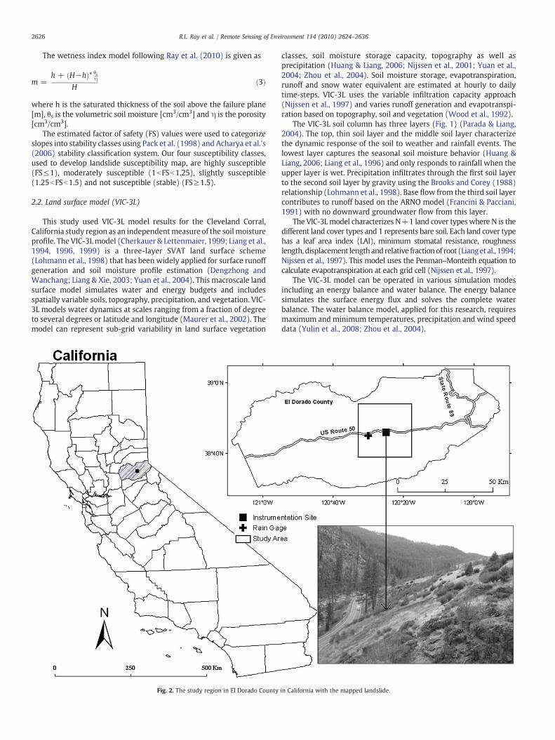
Fig. 2. The study region in El Dorado County

classes, soil moisture storage capacity, topography as well asprecipitation (Huang & Liang, 2006; Nijssen et al., 2001; Yuan et al.,2004; Zhou et al., 2004). Soil moisture storage, evapotranspiration,runoff and snow water equivalent are estimated at hourly to dailytime-steps. VIC-3L uses the variable infiltration capacity approach(Nijssen et al., 1997) and varies runoff generation and evapotranspi-ration based on topography, soil and vegetation (Wood et al., 1992).

The VIC-3L soil column has three layers (Fig. 1) (Parada & Liang,2004). The top, thin soil layer and the middle soil layer characterizethe dynamic response of the soil to weather and rainfall events. Thelowest layer captures the seasonal soil moisture behavior (Huang &Liang, 2006; Liang et al., 1996) and only responds to rainfall when theupper layer is wet. Precipitation infiltrates through the first soil layerto the second soil layer by gravity using the Brooks and Corey (1988)relationship (Lohmann et al., 1998). Base flow from the third soil layercontributes to runoff based on the ARNO model (Francini & Pacciani,1991) with no downward groundwater flow from this layer.

The VIC-3Lmodel characterizes N+1 land cover types where N is thedifferent land cover types and 1 represents bare soil. Each land cover typehas a leaf area index (LAI), minimum stomatal resistance, roughnesslength, displacement lengthandrelative fractionof root (Lianget al., 1994;Nijssen et al., 1997). This model uses the Penman–Monteith equation tocalculate evapotranspiration at each grid cell (Nijssen et al., 1997).

The VIC-3L model can be operated in various simulation modesincluding an energy balance and water balance. The energy balancesimulates the surface energy flux and solves the complete waterbalance. The water balance model, applied for this research, requiresmaximum and minimum temperatures, precipitation and wind speeddata (Yulin et al., 2008; Zhou et al., 2004).

in California with the mapped landslide.

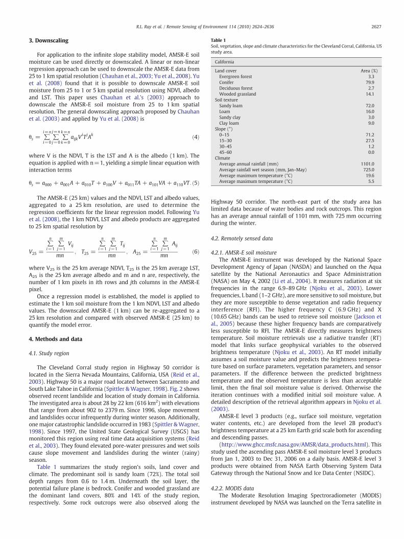
Table 1Soil, vegetation, slope and climate characteristics for the Cleveland Corral, California, USstudy area.

California

Land cover Area (%)Evergreen forest 3.3Conifer 79.9Deciduous forest 2.7Wooded grassland 14.1

Soil textureSandy loam 72.0Loam 16.0Sandy clay 3.0Clay loam 9.0

Slope (°)0–15 71.215–30 27.530–45 1.245–60 0.0

ClimateAverage annual rainfall (mm) 1101.0Average rainfall wet season (mm, Jan–May) 725.0Average maximum temperature (°C) 19.6Average maximum temperature (°C) 5.5

2627R.L. Ray et al. / Remote Sensing of Environment 114 (2010) 2624–2636

3. Downscaling

For application to the infinite slope stability model, AMSR-E soilmoisture can be used directly or downscaled. A linear or non-linearregression approach can be used to downscale the AMSR-E data from25 to 1 km spatial resolution (Chauhan et al., 2003; Yu et al., 2008). Yuet al. (2008) found that it is possible to downscale AMSR-E soilmoisture from 25 to 1 or 5 km spatial resolution using NDVI, albedoand LST. This paper uses Chauhan et al.'s (2003) approach todownscale the AMSR-E soil moisture from 25 to 1 km spatialresolution. The general downscaling approach proposed by Chauhanet al. (2003) and applied by Yu et al. (2008) is

θs = ∑i=n

i=0∑j=n

j=0∑k=n

k=0aijkV

iTjAk ð4Þ

where V is the NDVI, T is the LST and A is the albedo (1 km). Theequation is applied with n=1, yielding a simple linear equation withinteraction terms

θs = a000 + a001A + a010T + a100V + a011TA + a101VA + a110VT: ð5Þ

The AMSR-E (25 km) values and the NDVI, LST and albedo values,aggregated to a 25 km resolution, are used to determine theregression coefficients for the linear regression model. Following Yuet al. (2008), the 1 km NDVI, LST and albedo products are aggregatedto 25 km spatial resolution by

V25 =∑n

i=1∑m

j=1Vij

mn; T25 =

∑n

i=1∑m

j=1Tij

mn; A25 =

∑n

i=1∑m

j=1Aij

mnð6Þ

where V25 is the 25 km average NDVI, T25 is the 25 km average LST,A25 is the 25 km average albedo and m and n are, respectively, thenumber of 1 km pixels in ith rows and jth columns in the AMSR-Epixel.

Once a regression model is established, the model is applied toestimate the 1 km soil moisture from the 1 km NDVI, LST and albedovalues. The downscaled AMSR-E (1 km) can be re-aggregated to a25 km resolution and compared with observed AMSR-E (25 km) toquantify the model error.

4. Methods and data

4.1. Study region

The Cleveland Corral study region in Highway 50 corridor islocated in the Sierra Nevada Mountains, California, USA (Reid et al.,2003). Highway 50 is a major road located between Sacramento andSouth Lake Tahoe in California (Spittler &Wagner, 1998). Fig. 2 showsobserved recent landslide and location of study domain in California.The investigated area is about 28 by 22 km (616 km2) with elevationsthat range from about 902 to 2379 m. Since 1996, slope movementand landslides occur infrequently during winter season. Additionally,onemajor catastrophic landslide occurred in 1983 (Spittler &Wagner,1998). Since 1997, the United State Geological Survey (USGS) hasmonitored this region using real time data acquisition systems (Reidet al., 2003). They found elevated pore-water pressures and wet soilscause slope movement and landslides during the winter (rainy)season.

Table 1 summarizes the study region's soils, land cover andclimate. The predominant soil is sandy loam (72%). The total soildepth ranges from 0.6 to 1.4 m. Underneath the soil layer, thepotential failure plane is bedrock. Conifer and wooded grassland arethe dominant land covers, 80% and 14% of the study region,respectively. Some rock outcrops were also observed along the

Highway 50 corridor. The north-east part of the study area haslimited data because of water bodies and rock outcrops. This regionhas an average annual rainfall of 1101 mm, with 725 mm occurringduring the winter.

4.2. Remotely sensed data

4.2.1. AMSR-E soil moistureThe AMSR-E instrument was developed by the National Space

Development Agency of Japan (NASDA) and launched on the Aquasatellite by the National Aeronautics and Space Administration(NASA) on May 4, 2002 (Li et al., 2004). It measures radiation at sixfrequencies in the range 6.9–89 GHz (Njoku et al., 2003). Lowerfrequencies, L band (1–2 GHz), aremore sensitive to soil moisture, butthey are more susceptible to dense vegetation and radio frequencyinterference (RFI). The higher frequency C (6.9 GHz) and X(10.65 GHz) bands can be used to retrieve soil moisture (Jackson etal., 2005) because these higher frequency bands are comparativelyless susceptible to RFI. The AMSR-E directly measures brightnesstemperature. Soil moisture retrievals use a radiative transfer (RT)model that links surface geophysical variables to the observedbrightness temperature (Njoku et al., 2003). An RT model initiallyassumes a soil moisture value and predicts the brightness tempera-ture based on surface parameters, vegetation parameters, and sensorparameters. If the difference between the predicted brightnesstemperature and the observed temperature is less than acceptablelimit, then the final soil moisture value is derived. Otherwise theiteration continues with a modified initial soil moisture value. Adetailed description of the retrieval algorithm appears in Njoku et al.(2003).

AMSR-E level 3 products (e.g., surface soil moisture, vegetationwater contents, etc.) are developed from the level 2B product'sbrightness temperature at a 25 km Earth grid scale both for ascendingand descending passes.

(http://www.ghcc.msfc.nasa.gov/AMSR/data_products.html). Thisstudy used the ascending pass AMSR-E soil moisture level 3 productsfrom Jan 1, 2003 to Dec 31, 2006 on a daily basis. AMSR-E level 3products were obtained from NASA Earth Observing System DataGateway through the National Snow and Ice Data Center (NSIDC).

4.2.2. MODIS dataThe Moderate Resolution Imaging Spectroradiometer (MODIS)

instrument developed by NASA was launched on the Terra satellite in

2628 R.L. Ray et al. / Remote Sensing of Environment 114 (2010) 2624–2636

December 1999 and on the Aqua satellite in May 2002 (Wang et al.,2009). MODIS can collect information both in the morning and in theafternoon as Terra is scheduled to pass from north to south across theequator in the morning and Aqua is scheduled to pass from south tonorth in the afternoon. Even though Terra andAqua satellites pass in themorning and in the afternoon, respectively, the temporal resolution ofMODIS products is only every 1 to 2 days (Luo et al., 2008). MODIS dataare available at spatial resolutions of 0.25, 0.50, and 1.0 km as well ascoarser resolutions (Luo et al., 2008).

This study required NDVI, albedo and LST at a 1 km spatialresolution. The 1 km MODIS TERRA albedo (MCD43B3), NDVI(MYD13A2) and LST (MYD11A1) products were used to downscalethe AMSR-E surface soil moisture for 2005. Monthly LAI values, usedin VIC-3L model, were obtained from the MODIS. The MOD15A2, 8-day composite LAI values were averaged to monthly values. Thesedata are available as tiles in the Sinusoidal (SIN) projection. All thesedata were re-projected into a geographical projection.

4.3. Model data

The soil and vegetation parameter required for the slope stabilitymodel were obtained from the States Soil Geographic (STATSGO) (SoilSurvey Staff, 2008), Land Data Assimilation System (LDAS; Mitchell etal., 2004) as well as from the literature (Table 2). Root cohesionenhances the shear strength of soil and acts as a resisting force againstsliding. Root cohesion values for each vegetation class were adaptedfrom Sidle and Ochiai (2006). The unit soil weight (saturated and dry)was calculated based on the soil moisture, soil porosity, and specificgravity of the soil samples usingmethods adapted by Ray et al. (2010).Each soil type was assigned soil cohesion and friction angle valuesbased on Deoja et al. (1991) and the slope of the retention curve fromClapp and Hornberger (1978). Similarly, soil bulk density, fieldcapacity, wilting point and saturated hydraulic conductivity valueswere from Miller and White (1998) and Dingman (2002). A 90 mSRTM digital elevation model (DEM) was used to calculate slopeangle.

For this region, validation data for landslide studies are difficult toobtain. Daily groundwater measurements were obtained from theUSGS which uses piezometers to measure the hydraulic head at one ofthe active landslides in the region. (Mark Reid, USGS, personalcommunication, April 23, 2007). Previous research indicates that over600 small to large landslides have occurred in this study region (Reid

Table 2List of model parameters and sources by model.

Parameters Sources Model

Soil cohesion Deoja et al. (1991) Slope stabilitySoil porosity Dingman (2002) Slope stability and VIC-3LSoil texture STATSGO Slope stability and VIC-3LSoil depth STATSGO Slope stability and VIC-3LHydraulic conductivity STATSGO VIC-3LSoil bulk density Dingman (2002) Slope stability and VIC-3LAngle of internal friction Deoja et al. (1991) Slope stabilityAdditional load (surcharge) Ray (2004) Slope stabilityLand cover University of Maryland Slope stability and VIC-3LRoot cohesion Sidle and Ochiai (2006) Slope stabilityRoot depth LDAS VIC-3LRoot fraction LDAS VIC-3LVegetation roughness LDAS VIC-3LVegetation height LDAS VIC-3LLeaf area index (LAI) MODIS VIC-3LRainfall NCDC VIC-3LGroundwater USGS Slope stabilityTemperature NCDC VIC-3LWind speed NCDC VIC-3L

STATSGO=States Soil Geographic, LDAS=Land Data Assimilation System,USGS=United States Geological Survey, VIC-3L=Variable Infiltration Capacity-3Layers. NCDC=National Climatic Data Center.

et al., 2003; Spittler & Wagner, 1998). In addition, field observationsidentified 10 locations where failures had occurred prior to December2007. Table 4 lists slide locations and their physical characteristics.Observations show that most of the mapped landslides were locatedin woodland regions with sandy loam soil texture. The slopes of themapped landslides range from 24° to 37°.

4.4. Analysis methods

A course resolution AMSR-E (25 km) was downscaled to fine(1 km) resolution using MODIS LAI, albedo, and NDVI at 1 km spatialresolution. Using time series analysis, AMSR-E soil moisture at 25 kmresolution was compared with VIC-3l model surface soil moisture(layers 1 and 2) at 1 km spatial resolution to study the soil moisturevariability in study area. Because no in-situ soil moisture measure-ments were available, daily groundwater measurements were alsocompared with AMSR-E and VIC-3l model soil moisture. Themaximum model saturation day, 8 May, 2005, was identified todevelop landslide susceptibility map. To address the low variability ofAMSR-E soil moisture, downscaled AMSR-E soil moisture was scaledfrom residual soil moisture (minimum) to soil porosity (maximum).

This study uses a 90 m spatial resolution to calculate wetnessindex, dry unit soil weight, effective unit soil weight and factor ofsafety. The effective unit weight of soil was calculated using dry unitweight, wetness index, depth of soil, surcharge and slope angle(Eq. (2)). Wetness indices were calculated using Eq. (3) for modeledgroundwater depth on May 8, 2005 (maximum saturation) and thegroundwater table located at midpoint of the soil layer (halfsaturation) with the 1 km VIC-3L model vadose zone soil moisturevalues as well as the 1 and 25 km resolution AMSR-E soil moisturevalues.

Finally, safety factors were calculated for these two groundwaterpositions using VIC-3L model soil moisture and AMSR-E soil moisture.Theoretically, landslides occur when the safety factor is less than one.The estimated FS values were used to categorize slopes into the fourlandslide susceptibility classes; highly susceptible, moderately sus-ceptible, slightly susceptible and stable.

5. Results and discussion

5.1. Downscaling AMSR-E soil moisture

AMSR-E soil moisture at Cleveland Coral, California was down-scaled from 25 to 1 km using daily data from January 1 to December31, 2005. The 1 km NDVI, LST, and albedo were aggregated to 25 kmresolution using Eq. (6). The observed maximum LST, albedo andNDVI are, respectively, 51 °C, 0.94 and 0.93. The minimum are,respectively, −20 °C, 0.01 and −0.14. The AMSR-E (25 km) wasregressed with aggregated NDVI, LST and albedo values (Eq. (5)). Theestimated regression coefficients for each individual parameter andinteraction term were used to develop Eq. (7). The regression modelwhich best fits the soil moisture observation is

θs = −1:426 + 4:169 A + 0:006 T + 2:254 V−0:017 TA

+ 0:781 VA−0:009 VT

ð7Þ

This regression model provided a good fit with an R2 of 0.73, a rootmean square error (RMSE) of 0.009 cm3/cm3 and p-values less than0.0001 for all independent variables. As anticipated, soil moistureincreases with increasing vegetation index. However, the modelassociates wetter soils with higher albedo values and higher tempera-tures in contrast to typically observed physical relationships. Becausethis equation describes the annual cycle of surface and moistureconditions, the model interaction terms are very important. The soilmoisture variability is described primarily by the vegetation indexchanges and the interactions between vegetation and albedo. The

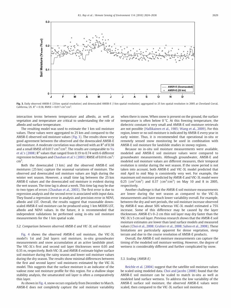
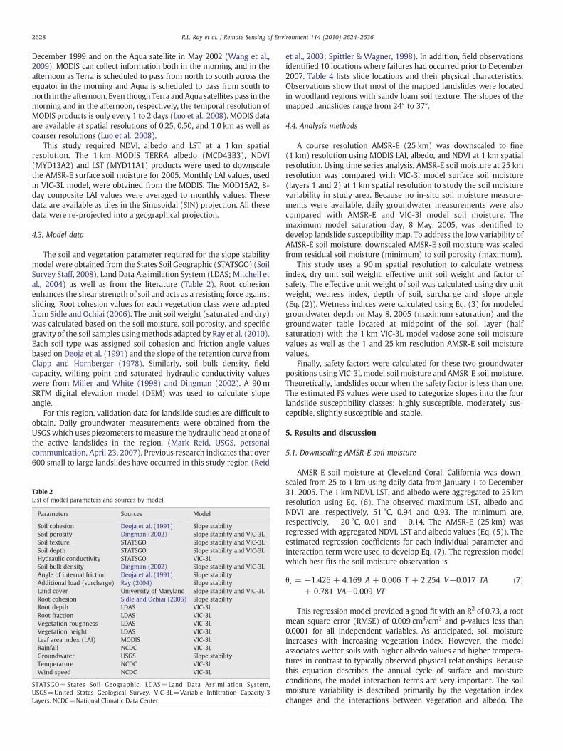
Fig. 3. Daily observed AMSR-E (25km spatial resolution) and downscaled AMSR-E (1km spatial resolution) aggregated to 25 km spatial resolution in 2005 at Cleveland Corral,California, US. R2=0.58, RMSE=0.017 cm3/cm3.

2629R.L. Ray et al. / Remote Sensing of Environment 114 (2010) 2624–2636

interaction terms between temperature and albedo, as well asvegetation and temperature are critical to understanding the role ofalbedo and surface temperature.

The resulting model was used to estimate the 1 km soil moisturevalues. These values were aggregated to 25 km and compared to theAMSR-E observed soil moisture values (Fig. 3). The results show verygood agreement between the observed and the downscaled AMSR-Esoil moisture. A moderate correlation was observed with an R2 of 0.58and a small RMSE of 0.017 cm3/cm3. The results are comparable to Yuet al.'s (2008) R2 values that ranged from 0.19 to 0.74 with 6 differentregression techniques and Chauhan et al.'s (2003) RMSE of 0.016 cm3/cm3.

Both the downscaled (1 km) and the observed AMSR-E soilmoistures (25 km) capture the seasonal variations of moisture. Theobserved and downscaled soil moisture values are high during thewinter wet season. However, a small time lag between the 25 kmAMSR-E values and the downscaled soil moisture is evident duringthe wet season. The time lag is about a week. This time lag may be dueto two types of errors (Chauhan et al., 2003). The first error is due toregression analysis and the second error is associated with input data.They found a regression error in analysis and precision error in NDVI,albedo and LST. Overall, the results suggest that reasonable down-scaled AMSR-E soil moisture can be produced using 1 km MODIS LST,albedo and NDVI values. In the future, it is recommended thatindependent validations be performed using in-situ soil moisturemeasurements for the 1 km spatial scale.

5.2. Comparison between observed AMSR-E and VIC-3L soil moisture

Fig. 4 shows the observed AMSR-E soil moisture, the VIC-3Lmodel's 1st and 2nd layers soil moisture, in-situ groundwatermeasurements and snow accumulation at an active landslide pixel.The VIC-3L's first and second soil layer thicknesses were 0.05 and0.35 m, respectively. Both VIC-3L and AMSR-E estimate higher surfacesoil moisture during the rainy season and lower soil moisture valuesduring the dry season. The results show minimal differences betweenthe first and second layers' soil moistures estimated by the VIC-3Lmodel. This suggests that the surface moisture is an indicator of thevadose zone soil moisture profile for this region. For a shallow slopestability analysis, the unsaturated soil layer is often a comparativelythin layer.

As shown in Fig. 4, snow occurs regularly fromDecember toMarch.AMSR-E does not completely capture the soil moisture variability

when there is snow. When snow is present on the ground, the surfacetemperature is often below 0 °C. At this freezing temperature, thedielectric constant is very small and AMSR-E soil moisture retrievalsare not possible (Hallikainen et al., 1985; Wang et al., 2009). For thisregion, lower or no soil moisture is indicated by AMSR-E every year inearly winter. Thus, it is recommended that operational in-situ orremotely sensed snow monitoring be used in combination withAMSR-E soil moisture for landslide studies in snowy regions.

Because no in-situ soil moisture measurements were available,modeled and AMSR-E soil moisture values were compared togroundwater measurements. Although groundwater, AMSR-E andmodeled soil moisture values are different measures, their temporalevolution is similar during the wet season. If the snow period is nottaken into account, both AMSR-E and VIC-3L model predicted thatmid April to mid May is consistently very wet. For example, themaximum soil moisture predicted by AMSR-E and VIC-3L model were0.25 (cm3/cm3) and 0.37 (cm3/cm3) on May 10 and 8 in 2005,respectively.

Another challenge is that the AMSR-E soil moisture measurementsare lower during the wet season as compared to the VIC-3Lmeasurements and have much lower variability overall. For example,between the dry and wet periods, the soil moisture increase observedby AMSR-E was about 50% whereas VIC-3L model estimated a 75%increase. Some of this difference may be caused by the layerthicknesses. AMSR-E's 0–2 cm thin soil layer may dry faster than theVIC-3L's 5 cm soil layer. Previous research shows that the AMSR-E soilmoisture estimates are lower than land surface models and measuredvalues (Choi et al., 2008; Gruhier et al., 2008; Sahoo et al., 2008). Theselimitations are particularly apparent for dense vegetation, steepterrain and due to the course resolution of AMSR-E products.

Overall, the AMSR-E soil moisture measurements can capture thetiming of the modeled soil moisture wetting. However, the degree ofwetness is considerably different and further complicated by snow.

5.3. Scaling (AMSR-E)

Reichle et al. (2004) suggest that the satellite soil moisture valuesbe scaled using modeled data. Choi and Jacobs (2008) found that theAMSR-E soil moisture can be scaled to match in-situ as well asmodeled land surface wetness. To address the low variability of theAMSR-E surface soil moisture, the observed AMSR-E values werescaled, then compared to the VIC-3L surface soil moisture.

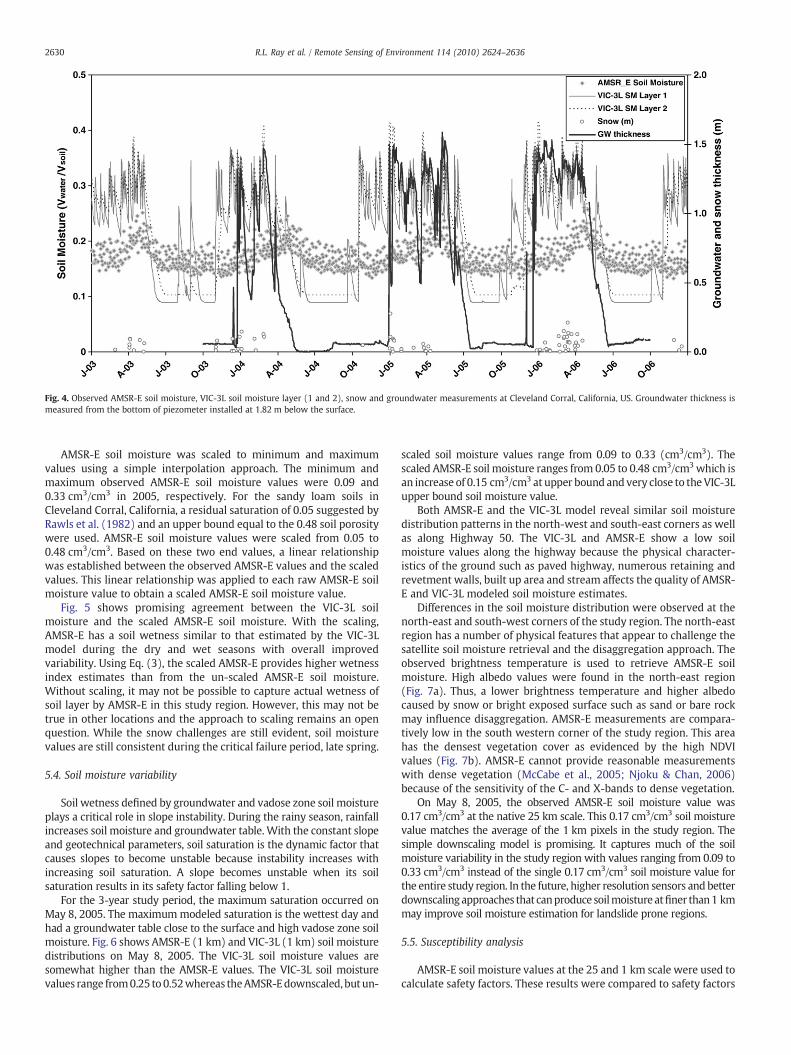
Fig. 4. Observed AMSR-E soil moisture, VIC-3L soil moisture layer (1 and 2), snow and groundwater measurements at Cleveland Corral, California, US. Groundwater thickness ismeasured from the bottom of piezometer installed at 1.82 m below the surface.

2630 R.L. Ray et al. / Remote Sensing of Environment 114 (2010) 2624–2636

AMSR-E soil moisture was scaled to minimum and maximumvalues using a simple interpolation approach. The minimum andmaximum observed AMSR-E soil moisture values were 0.09 and0.33 cm3/cm3 in 2005, respectively. For the sandy loam soils inCleveland Corral, California, a residual saturation of 0.05 suggested byRawls et al. (1982) and an upper bound equal to the 0.48 soil porositywere used. AMSR-E soil moisture values were scaled from 0.05 to0.48 cm3/cm3. Based on these two end values, a linear relationshipwas established between the observed AMSR-E values and the scaledvalues. This linear relationship was applied to each raw AMSR-E soilmoisture value to obtain a scaled AMSR-E soil moisture value.

Fig. 5 shows promising agreement between the VIC-3L soilmoisture and the scaled AMSR-E soil moisture. With the scaling,AMSR-E has a soil wetness similar to that estimated by the VIC-3Lmodel during the dry and wet seasons with overall improvedvariability. Using Eq. (3), the scaled AMSR-E provides higher wetnessindex estimates than from the un-scaled AMSR-E soil moisture.Without scaling, it may not be possible to capture actual wetness ofsoil layer by AMSR-E in this study region. However, this may not betrue in other locations and the approach to scaling remains an openquestion. While the snow challenges are still evident, soil moisturevalues are still consistent during the critical failure period, late spring.

5.4. Soil moisture variability

Soil wetness defined by groundwater and vadose zone soil moistureplays a critical role in slope instability. During the rainy season, rainfallincreases soil moisture and groundwater table. With the constant slopeand geotechnical parameters, soil saturation is the dynamic factor thatcauses slopes to become unstable because instability increases withincreasing soil saturation. A slope becomes unstable when its soilsaturation results in its safety factor falling below 1.

For the 3-year study period, the maximum saturation occurred onMay 8, 2005. The maximummodeled saturation is the wettest day andhad a groundwater table close to the surface and high vadose zone soilmoisture. Fig. 6 shows AMSR-E (1 km) and VIC-3L (1 km) soil moisturedistributions on May 8, 2005. The VIC-3L soil moisture values aresomewhat higher than the AMSR-E values. The VIC-3L soil moisturevalues range from0.25 to 0.52whereas theAMSR-Edownscaled, butun-

scaled soil moisture values range from 0.09 to 0.33 (cm3/cm3). Thescaled AMSR-E soil moisture ranges from 0.05 to 0.48 cm3/cm3which isan increase of 0.15 cm3/cm3 at upper bound and very close to the VIC-3Lupper bound soil moisture value.

Both AMSR-E and the VIC-3L model reveal similar soil moisturedistribution patterns in the north-west and south-east corners as wellas along Highway 50. The VIC-3L and AMSR-E show a low soilmoisture values along the highway because the physical character-istics of the ground such as paved highway, numerous retaining andrevetment walls, built up area and stream affects the quality of AMSR-E and VIC-3L modeled soil moisture estimates.

Differences in the soil moisture distribution were observed at thenorth-east and south-west corners of the study region. The north-eastregion has a number of physical features that appear to challenge thesatellite soil moisture retrieval and the disaggregation approach. Theobserved brightness temperature is used to retrieve AMSR-E soilmoisture. High albedo values were found in the north-east region(Fig. 7a). Thus, a lower brightness temperature and higher albedocaused by snow or bright exposed surface such as sand or bare rockmay influence disaggregation. AMSR-E measurements are compara-tively low in the south western corner of the study region. This areahas the densest vegetation cover as evidenced by the high NDVIvalues (Fig. 7b). AMSR-E cannot provide reasonable measurementswith dense vegetation (McCabe et al., 2005; Njoku & Chan, 2006)because of the sensitivity of the C- and X-bands to dense vegetation.

On May 8, 2005, the observed AMSR-E soil moisture value was0.17 cm3/cm3 at the native 25 km scale. This 0.17 cm3/cm3 soil moisturevalue matches the average of the 1 km pixels in the study region. Thesimple downscaling model is promising. It captures much of the soilmoisture variability in the study region with values ranging from 0.09 to0.33 cm3/cm3 instead of the single 0.17 cm3/cm3 soil moisture value forthe entire study region. In the future, higher resolution sensors and betterdownscalingapproaches that canproduce soilmoistureatfiner than1 kmmay improve soil moisture estimation for landslide prone regions.

5.5. Susceptibility analysis

AMSR-E soil moisture values at the 25 and 1 km scale were used tocalculate safety factors. These results were compared to safety factors

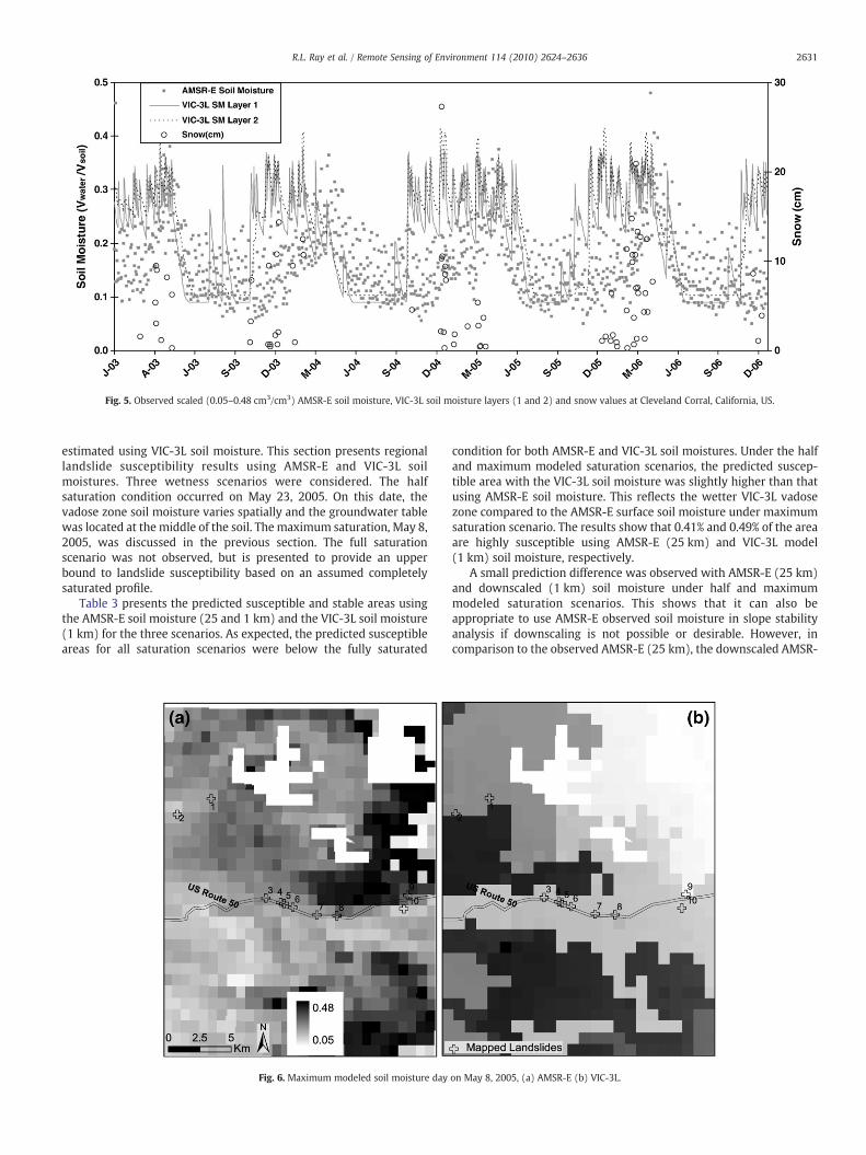
Fig. 5. Observed scaled (0.05–0.48 cm3/cm3) AMSR-E soil moisture, VIC-3L soil moisture layers (1 and 2) and snow values at Cleveland Corral, California, US.

2631R.L. Ray et al. / Remote Sensing of Environment 114 (2010) 2624–2636

estimated using VIC-3L soil moisture. This section presents regionallandslide susceptibility results using AMSR-E and VIC-3L soilmoistures. Three wetness scenarios were considered. The halfsaturation condition occurred on May 23, 2005. On this date, thevadose zone soil moisture varies spatially and the groundwater tablewas located at the middle of the soil. The maximum saturation, May 8,2005, was discussed in the previous section. The full saturationscenario was not observed, but is presented to provide an upperbound to landslide susceptibility based on an assumed completelysaturated profile.

Table 3 presents the predicted susceptible and stable areas usingthe AMSR-E soil moisture (25 and 1 km) and the VIC-3L soil moisture(1 km) for the three scenarios. As expected, the predicted susceptibleareas for all saturation scenarios were below the fully saturated

Fig. 6. Maximum modeled soil moisture day

condition for both AMSR-E and VIC-3L soil moistures. Under the halfand maximum modeled saturation scenarios, the predicted suscep-tible area with the VIC-3L soil moisture was slightly higher than thatusing AMSR-E soil moisture. This reflects the wetter VIC-3L vadosezone compared to the AMSR-E surface soil moisture under maximumsaturation scenario. The results show that 0.41% and 0.49% of the areaare highly susceptible using AMSR-E (25 km) and VIC-3L model(1 km) soil moisture, respectively.

A small prediction difference was observed with AMSR-E (25 km)and downscaled (1 km) soil moisture under half and maximummodeled saturation scenarios. This shows that it can also beappropriate to use AMSR-E observed soil moisture in slope stabilityanalysis if downscaling is not possible or desirable. However, incomparison to the observed AMSR-E (25 km), the downscaled AMSR-

on May 8, 2005, (a) AMSR-E (b) VIC-3L.

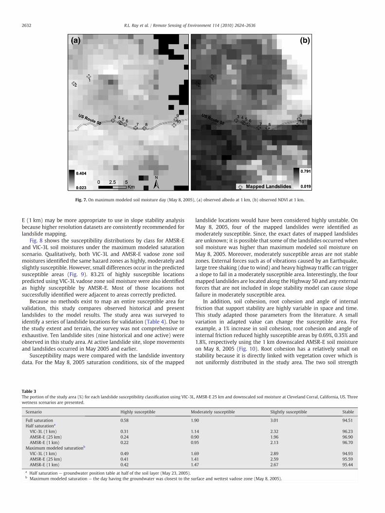
Fig. 7. On maximum modeled soil moisture day (May 8, 2005), (a) observed albedo at 1 km, (b) observed NDVI at 1 km.

2632 R.L. Ray et al. / Remote Sensing of Environment 114 (2010) 2624–2636

E (1 km) may be more appropriate to use in slope stability analysisbecause higher resolution datasets are consistently recommended forlandslide mapping.

Fig. 8 shows the susceptibility distributions by class for AMSR-Eand VIC-3L soil moistures under the maximum modeled saturationscenario. Qualitatively, both VIC-3L and AMSR-E vadose zone soilmoistures identified the same hazard zones as highly, moderately andslightly susceptible. However, small differences occur in the predictedsusceptible areas (Fig. 9). 83.2% of highly susceptible locationspredicted using VIC-3L vadose zone soil moisture were also identifiedas highly susceptible by AMSR-E. Most of those locations notsuccessfully identified were adjacent to areas correctly predicted.

Because no methods exist to map an entire susceptible area forvalidation, this study compares observed historical and presentlandslides to the model results. The study area was surveyed toidentify a series of landslide locations for validation (Table 4). Due tothe study extent and terrain, the survey was not comprehensive orexhaustive. Ten landslide sites (nine historical and one active) wereobserved in this study area. At active landslide site, slope movementsand landslides occurred in May 2005 and earlier.

Susceptibility maps were compared with the landslide inventorydata. For the May 8, 2005 saturation conditions, six of the mapped

Table 3The portion of the study area (%) for each landslide susceptibility classification using VIC-3Lwetness scenarios are presented.

Scenario Highly susceptible M

Full saturation 0.58 1.Half saturationa

VIC-3L (1 km) 0.31 1.AMSR-E (25 km) 0.24 0.AMSR-E (1 km) 0.22 0.

Maximum modeled saturationb

VIC-3L (1 km) 0.49 1.AMSR-E (25 km) 0.41 1.AMSR-E (1 km) 0.42 1.

a Half saturation — groundwater position table at half of the soil layer (May 23, 2005).b Maximum modeled saturation — the day having the groundwater was closest to the su

landslide locations would have been considered highly unstable. OnMay 8, 2005, four of the mapped landslides were identified asmoderately susceptible. Since, the exact dates of mapped landslidesare unknown; it is possible that some of the landslides occurred whensoil moisture was higher than maximum modeled soil moisture onMay 8, 2005. Moreover, moderately susceptible areas are not stablezones. External forces such as of vibrations caused by an Earthquake,large tree shaking (due to wind) and heavy highway traffic can triggera slope to fail in a moderately susceptible area. Interestingly, the fourmapped landslides are located along the Highway 50 and any externalforces that are not included in slope stability model can cause slopefailure in moderately susceptible area.

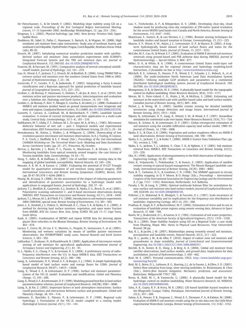
In addition, soil cohesion, root cohesion and angle of internalfriction that support stability are highly variable in space and time.This study adapted those parameters from the literature. A smallvariation in adapted value can change the susceptible area. Forexample, a 1% increase in soil cohesion, root cohesion and angle ofinternal friction reduced highly susceptible areas by 0.69%, 0.35% and1.8%, respectively using the 1 km downscaled AMSR-E soil moistureon May 8, 2005 (Fig. 10). Root cohesion has a relatively small onstability because it is directly linked with vegetation cover which isnot uniformly distributed in the study area. The two soil strength

, AMSR-E 25 km and downscaled soil moisture at Cleveland Corral, California, US. Three

oderately susceptible Slightly susceptible Stable

90 3.01 94.51

14 2.32 96.2390 1.96 96.9095 2.13 96.70

69 2.89 94.9341 2.59 95.5947 2.67 95.44

rface and wettest vadose zone (May 8, 2005).

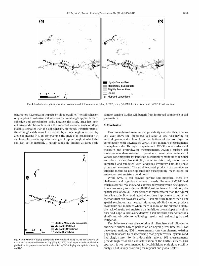
Fig. 8. Landslide susceptibility map for maximum modeled saturation day (May 8, 2005) using (a) AMSR-E soil moisture and (b) VIC-3L soil moisture.

2633R.L. Ray et al. / Remote Sensing of Environment 114 (2010) 2624–2636

parameters have greater impacts on slope stability. The soil cohesiononly applies to cohesive soil whereas frictional angle applies both tocohesive and cohesionless soils. Because the study area has bothcohesive and cohesionless soils, the impact of frictional angle on slopestability is greater than the soil cohesion. Moreover, the major part ofthe driving/destabilizing force caused by a slope angle is resisted byangle of internal friction. For example, the angle of internal friction ina cohesionless soil is equal to the angle of repose (angle at which thesoil can settle naturally). Future landslide studies at large-scale

Fig. 9. Comparison of highly susceptible area predicted using VIC-3L and AMSR-E onmaximum modeled soil moisture day (May 8, 2005). Black squares indicate identicalpredictions. Gray squares are location identified by VIC-3L highly susceptible, but not byAMSR-E.

remote-sensing studies will benefit from improved confidence in soilparameters.

6. Conclusion

This research used an infinite slope stability model with a pervioussoil layer above the impervious soil layer or bed rock having novertical groundwater flow from the bottom of the soil layer incombination with downscaled AMSR-E soil moisture measurementsto map landslides. Through comparisons to VIC-3L model surface soilmoisture and groundwater measurements, AMSR-E surface soilmoisture was demonstrated to provide a quantitative estimate ofvadose zone moisture for landslide susceptibility mapping at regionaland global scales. Susceptibility maps for this study region werecompared and validated with landslides inventory data and showpromising agreement. The satellite-based products can provide anefficient means to develop landslide susceptibility maps based onantecedent soil moisture conditions.

While AMSR-E can provide surface soil moisture, there arechallenges and significant research needs. Because AMSR-E hadmuch lower soil moisture and less variability than would be expected,it was necessary to scale the AMSR-E soil moisture. In addition, thespatial scale of AMSR-E observations is much greater than the typicallandslide scale. Downscaling provides some improvement, but bettermethods that can downscale AMSR-E soil moisture to finer than 1 kmspatial resolution, are needed. Moreover, AMSR-E cannot producereasonable soil moisture when there is snow on the surface. Finally,the lack of in-situ soil moisture on landslides prone slopes as well asobserved slope failures coincident with soil moisture observations is asignificant obstacle to validating results and enhancing hazardmitigation.

The ability to capture the evolution of soil moisture will allow us toanticipate critical hazard periods on an ongoing, real time basis. Fordeveloped nations, EOS measurements can complement existingphysical databases by characterizing changing terrestrial systems andhydrologic stores. For less data rich regions, EOS measurementsprovide high resolution characterization of the Earth's surface. Thisapproach is not recommended for local/hillslope scale slope stabilityanalysis, but is very promising for regional and global scales.

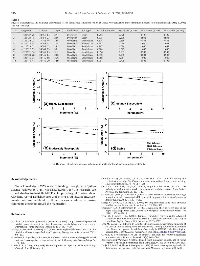
Table 4Physical characteristics and estimated safety factor (FS) of the mapped landslide's region. FS values were calculated under maximum modeled saturation conditions (May 8, 2005)and full saturation.

S.N. Longitude Latitude Slope (°) Land cover Soil types FS: Full saturation FS: VIC-3L (1 km) FS: AMSR-E (1 km) FS: AMSR-E (25 km)

1 −120° 27′ 26″ 38° 51′ 03″ 27.4 Evergreen Loam 0.753 0.770 0.797 0.7992 −120° 29′ 18″ 38° 50′ 23″ 28.6 Evergreen Loam 0.875 0.896 0.933 0.9313 −120° 24′ 22″ 38° 46′ 46″ 32.5 Woodland Sandy loam 0.815 0.838 0.861 0.8644 −120° 23′ 34″ 38° 46′ 37″ 27.4 Woodland Sandy loam 0.987 1.016 1.040 1.0475 −120° 23′ 23″ 38° 46′ 33″ 24.1 Woodland Sandy loam 0.997 1.026 1.050 1.0586 −120° 22′ 53″ 38° 46′ 23″ 36.1 Woodland Sandy loam 0.988 1.012 1.040 1.0407 −120° 21′ 34″ 38° 46′ 05″ 31.1 Woodland Sandy loam 0.856 0.881 0.905 0.9088 −120° 20′ 28″ 38° 46′ 04″ 29.6 Woodland Sandy loam 0.939 0.965 0.994 0.9929 −120° 16′ 33″ 38° 46′ 58″ 36.6 Woodland Sandy loam 0.988 1.014 1.025 1.04010 −120° 16′ 47″ 38° 46′ 20″ 34.9 Woodland Sandy loam 0.751 0.775 0.802 0.796

Fig. 10. Impact of soil cohesion, root cohesion and angle of internal friction on slope instability.

2634 R.L. Ray et al. / Remote Sensing of Environment 114 (2010) 2624–2636

Acknowledgements

We acknowledge NASA's research funding through Earth SystemScience Fellowship, Grant No: NNG05GP66H, for this research. Wewould also like to thank Dr. M.E. Reid for providing information aboutCleveland Corral Landslide area and in-situ groundwater measure-ments. We are indebted to three reviewers whose extensivecomments greatly improved the manuscript.

References

Abdallah, C., Chowrowicz, J., Bouheir, R., & Dhont, D. (2007). Comparative use of processedsatellite images in remote sensing of mass movements: Lebanon as a case study.International Journal of Remote Sensing, 28(19), 4409−4427.

Acharya, G., De Smedt, F., & Long, N. T. (2006). Assessing landslide hazard in GIS: A casestudy from Rasuwa, Nepal. Bulletin of Engineering Geology and the Environment, 65(1),99−107.

Brarddinoni, F., Slaymaker, O., &Hassan,M. A. (2003). Landslide inventory in rugged forestedwatershed: A comparison between air-photo and field survey data. Geomorphology, 54,179−196.

Brooks, R. H., & Corey, A. T. (1988). Hydraulic properties of porous media. Hydrol. Pap.Colorado State University, 3.

Canuti, P., Casagli, N., Ermini, L., Fanti, R., & Farina, P. (2004). Landslide activity as ageoindicator in Italy: Significance and new perspectives from remote sensing.Environmental Geology, 45(7), 907−919.

Carrara, A., Cadinali, M., Detti, R., Guzzetti, F., Pasqui, F., & Reichenbach, P. (1991). GIStechniques and statistical models in evaluating landslide hazard. Earth SurfaceProcesses and Landforms, 16, 427−445.

Chauhan, N. S., Miler, S., & Aradny, P. (2003). Spaceborn soil moisture estimation at highresolution: A microwave-optical/IR synergistic approach. International Journal ofRemote Sensing, 24(22), 4599−4622.

Cheng, K. S., Wei, C., & Chang, S. C. (2004). Locating landslides using multi-temporalsatellite images. Advances in Space Research, 33, 296−301.

Cherkauer, K. A., & Lettenmaier, D. P. (1999). Hydrologic effect of frozen soils in theupper Mississippi river basin. Journal of Geophysical Research-Atmospheres, 104(D16), 19599−19610.

Choi, M., & Jacobs, J. M. (2008). Temporal variability corrections for AdvancedMicrowave Scanning Radiometer E (AMSR-E) surface soil moisture: Case study inLittle River Region, Georgia, U.S.. Sensors, 8, 2617−2627.

Choi, M., Jacobs, J. M., & Bosch, D. D. (2008). Remote sensing observatory validation ofsurface soil moisture using Advanced Microwave Scanning Radiometer E, CommonLand Model, and ground based data: Case study in SMEX03 Little River Region,Georgia, U.S.. Water Resources Research, 44, W08421. doi:10.1029/2006WR005578.

Clapp, R. B., & Hornberger, G. M. (1978). Empirical equations for some soil hydrologicproperties. Water Resources Research, 14(4), 601−604.

Dengzhong, Z, & Wanchang, Z. (2005). Rainfall-runoff simulation using the VIC-3L modelover the Heihe River mountainous basin, China. IEEE, 0-7803-9050-4/05, 4391-4394.

Deoja, B. B., Dhital,M., Thapa,B., &Wagner,A. (1991).Mountain risk engineeringhandbook.Kathmandu: International Centre for Integrated Mountain Development (ICIMOD).

2635R.L. Ray et al. / Remote Sensing of Environment 114 (2010) 2624–2636

De Vleeschauwer, C., & De Smedt, F. (2002). Modeling slope stability using GIS on aregional scale. Proceedings of the first Geological Belgica International Meeting,Leuven, 11–15 September 2002. Aardkundige Mededelingen, 12. (pp. 253−256).

Dingman, S. L. (2002). Physical hydrology (pp. 646). New Jersey: Prentice Hall, UpperSaddle River.

Doubkova, M., Sabel, D., Pathe, C., Hasenauer, S., Bartsch, A., & Wagner, W. (2008). Highresolution soil moisture from radar instruments: Study area of northeast Austria andsoutheast CzechRepublic. HydroPredict-Prague, CzechRepublic; Bruthans-Kovar-Hrkal(eds), 89–92.

Drusch, M. (2007). Initializing numerical weather prediction models with satellite-derived surface soil moisture: Data assimilation experiments with ECMWF'sIntegrated Forecast System and the TMI soil moisture data set. Journal ofGeophysical Research, 112, D03102. doi:10.1029/2006JD007478.

Francini, M., & Pacciani, M. (1991). Comparative analysis of several conceptual rainfall-runoff models. Journal of Hydrology, 122, 161−219.

Gao, H., Wood, E. F., Jackson, T. J., Drusch, M., & Bindlish, R. (2006). Using TRMM/TMI toretrieve surface soil moisture over the southern United States from 1998 to 2002.Journal of Hydrometeorology, 7, 23−38.

Gorsevski, P. V., Gessler, P. E., & Jankowski, P. (2003). Integrating a fuzzy k-meansclassification and a Bayesian approach for spatial prediction of landslide hazard.Journal of Geographical Systems, 5(3), 223−251.

Gruhier, C., de Rosnay, P., Hasenauer, S., Holmes, T., de Jeu, R., Kerr, Y., et al. (2010). Soilmoisture active and passive microwave products: intercomparison and evaluationover a Sahelian site. Hydrology and Earth System Sciences, 14, 141−156.

Gruhier, C., de Rosnay, P., Kerr, Y., Mougin, E., Ceschia, E., & Calvet, J. C. (2008). Evaluation ofAMSR-E soil moisture product based on ground measurements over temperate andsemi-arid regions.Geophysical Research Letters, 35, L10405. doi:10.1029/2008GL033330.

Guzzetti, F., Carrara, A., Cardinali, M., & Reichenbach, P. (1999). Landslide hazardevaluation: A review of current techniques and their application in a multi-scalestudy, Central Italy. Geomorphology, 31(1–4), 181−216.

Hallikainen, M. T., Ulaby, F. T., Dobson, M. C., El-rayes, M. A., &Wu, L. (1985). Microwavedielectric behavior of wet soil — part I: Empirical models and experimentalobservations. IEEE Transactions on Geoscience and Remote Sensing, GE-23(1), 25−34.

Hemakumara, M., Kalma, J., Walker, J., & Willgoose, G. (2004). Downscaling of lowresolution passive microwave soil moisture observations. In A. J. Teuling, H. Leijnse,P. A. Troch, J. Sheffield, & E. F. Wood (Eds.), Proceedings of the 2nd InternationalCAHMDA Workshop on: The Terrestrial Water Cycle: Modeling and Data AssimilationAcross Catchment Scales (pp. 25−27). Princeton, NJ, October.

Hervas, J., Barredo, J. I., Rosin, P. L., Pasuto, A., Mantovani, F., & Silvano, S. (2003).Monitoring landslides from optical remotely sensed imagery: the case history ofTessina landslide, Italy. Geomorphology, 54, 63−75.

Hong, Y., Adler, R., & Huffman, G. (2007). Use of satellite remote sensing data in themapping of global landslide susceptibility. Natural Hazards, 43, 245−256.

Hossain, A. K. M. A., & Easson, G. (2008). Evaluating the potential of VI-LST Trianglemodel for quantitative estimation of soil moisture using optical imagery. IEEEInternational Geosciences and Remote Sensing Symposium (IGARSS), Boston, USA(pp. III-47-50).978-1-4244-2808-3.

Huang, M., & Liang, X. (2006). On the assessment of the impact of reducing parametersand identification of parameter uncertainties for a hydrologic model withapplications to ungauged basins. Journal of Hydrology, 320, 37−61.

Jackson, T. J., Bindlish, R., Gasiewski, A. J., Stankov, B., Njoku, E. G., Bosch, D., et al. (2005).Polarimetric scanning radiometer C- and X-band microwave observations duringSMEX03. IEEE Transactions on Geoscience and Remote Sensing, 43(11), 2418−2430.

Jackson, T. J., Moran,M. S., & O'Neill, P. E. (2008). Introduction to soilmoisture experiments2004 (SMEX04) special issue. Remote Sensing of Environment, 112, 301−303.

Jones, L. A., Kimball, J. S., Podest, E., McDonald, K. C., Chan, S. K., & Njoku, E. G. (2009). Amethod for deriving land surface moisture, vegetation, and open water fractionfrom AMSRE. IEEE Int. Geosci. Rem. Sens. Symp. IGARSS '09, July 13–17, Cape Town,South Africa.

Kaab, A. (2005). Combination of SRTM3 and repeat ASTER data for deriving alpineglacier flow velocities in the Bhutan Himalaya. Remote Sensing of Environment, 94,463−474.

Lacava, T., Greco, M., Di Leo, E. V., Martino, G., Pergola, N., Sannazzaro, F., et al. (2005).Monitoring soil wetness variations by means of satellite passive microwaveobservations: the HYDROPTIMET study cases. Natural Hazards and Earth SystemSciences, 5, 583−592.

Lakhankar, T., Krakauer, N., & Khanbilvardi, R. (2009). Application of microwave remotesensing of soil moisture for agricultural applications. International Journal ofTerraspace Science and Engineering, 2(1), 81−91.

Li, L., Njoku, E. G., Chang, P. S., & Germain, K. S. (2004). A preliminary survey of radio-frequency interference over the U.S. in Aqua AMSR-E data. IEEE Transactions onGeoscience and Remote Sensing, 42(2), 380−390.

Liang, X., Lettenmaier, D. P., Wood, E. F., & Burges, S. J. (1994). A simple hydrologicallybased model of land surface water and energy fluxes for GSMs. Journal ofGeophysical Research, 99(D7), 14415−14428.

Liang, X., Wood, E. F., & Lettenmaier, D. P. (1996). Surface soil moisture parameter-ization of the VIC-2L model: Evaluation and modifications. Global and PlanetaryChange, 13, 195−206.

Liang,X.,Wood, E. F., & Lettenmaier, D. P. (1999).Modelinggroundheatflux in landsurfaceparameterization schemes. Journal of Geophysical Research, 104(D8), 9581−9600.

Liang, X., & Xie, Z. (2003). Important factors in land–atmosphere interactions: Surfacerunoff generations and interactions between surface and groundwater. Global andPlanetary Change, 38, 101−114.

Lohmann, D., Raschike, E., Nijssen, P., & Lettenmaier, D. P. (1998). Regional scalehydrology: I. Formulation of the VIC-2L model coupled to a routing model.Hydrological Sciences Journal, 43(1), 131−141.

Luo, Y., Trishchenko, A. P., & Khlopenkov, K. V. (2008). Developing clear-sky, cloudshadow mask for producing clear-sky composites at 250-meter spatial resolutionfor the seven MODIS land bands over Canada and North America. Remote Sensing ofEnvironment, 112, 4167−4185.

Mantovani, F., Soeters, R., & van Westen, C. J. (1996). Remote sensing techniques forlandslide studies and hazard zonation in Europe. Geomorphology, 15, 213−225.

Maurer, E. P., Wood, A. W., Adam, J. C., Lettenmaier, D. P., & Nijssen, B. (2002). A long-term hydrologically based dataset of land surface fluxes and states for theconterminous United States. Journal of Climate, 15, 3237−3251.

McCabe, M. F., Gao, H., &Wood, E. F. (2005). Evaluation of AMSR-E derived soil moistureretrievals using ground-based and PSR airborne data during SMEX02. Journal ofHydrometeorology — Special Edition, 6, 864−877.

Miller, D. A., & White, R. A. (1998). A conterminous United States multi-layer soilcharacteristics data set for regional climate and hydrology modeling.EarthInteractions, 2 [Available on-line at http://www.EarthInteractions.org].

Mitchell, K. E., Lohman, D., Houser, P. R., Wood, E. F., Schaake, J. C., Robock, A., et al.(2004). The multi-institution North American Land Data Assimilation System(NLDAS): Utilizing multiple GCIP products and parameters in a continentaldistributed hydrological modeling system. Journal of Geophysical Research, 109,Do7S90. doi:10.1029/2003JD003823.

Montgomery, D. R., & Dietrich, W. E. (1994). A physically based model for the topographiccontrol on shallow landsliding.Water Resources Research, 30(4), 1153−1171.

Moran, M. S., Peter-Lidard, C. D., Watts, J. M., & McElroy, S. (2004). Estimating soilmoisture at thewatershed scale with satellite-based radar and land surface models.Canadian Journal of Remote Sensing, 30(5), 805−826.

Nichol, J., & Wong, M. S. (2005). Satellite remote sensing for detailed landslideinventories using change detection and image fusion. International Journal ofRemote Sensing, 26(9), 1913−1926.

Nijssen, B., Lettenmaier, D. P., Liang, X., Wetzel, S. W., & Wood, E. F. (1997). Streamflowsimulation for continental-scale river basins.Water Resources Research, 33(4), 711−724.

Nijssen, B., Schnur, R., & Lettenmaier, D. P. (2001). Global retrospective estimation ofsoil moisture using the variable infiltration capacity land surface model, 1980–93.Journal of Climate, 14, 1790−1808.

Njoku, E. G., & Chan, S. K. (2006). Vegetation and surface roughness effects on AMSR-Eland observations. Remote Sensing of Environment, 100, 190−199.

Njoku, E. G., Jackson, T. J., & Koike T. (2000). AMSR-E Science Data Validation Plan (pp.76), version 2, 7/00.

Njoku, E. G., Jackson, T. J., Lakshmi, V., Chan, T. K., & Nghiem, S. V. (2003). Soil moistureretrieval from AMSR-E. IEEE Transactions on Geoscience and Remote Sensing, 412(2),215−229.

Oka, N. (1998). Application of photogrammetry to the field observation of failed slopes.Engineering Geology, 50, 85−100.

Ostir, K., Veljanovski, T., Podobanikar, T., & Stancic, Z. (2003). Application of satelliteremote sensing in natural hazard management: The Mount Mangart landslide casestudy. International Journal of Remote Sensing, 24(20), 3983−4002.

Pack, R. T., Tarboton, D. G., & Goodwin, C. N. (1998). The SINMAP approach to terrainstability mapping. In D. P. Moore, & O. Hungr (Eds.), Proceedings — InternationalCongress of the International Association for Engineering Geology and the Environment8, 2 (pp. 1157−1165). Rotterdam, Netherlands: A.A. Balkema.

Parada, L. M., & Liang, X. (2004). Optimal multiscale Kalman filter for assimilation fornear-surface soil moisture into land surface models. Journal of Geophysical Research,109, D24109. doi:10.1029/2004JD004745.

Pelletier, J. D., Malamud, B. D., Blodgett, T., & Turcotte, D. L. (1997). Scale-invariance ofsoil moisture variability and its implications for the frequency-size distribution oflandslides. Engineering Geology, 48(3–4), 255−268.

Pradhan, B., Singh, R. P., & Buchroithner, M. F. (2006). Estimation of stress and its use inevaluation of landslide prone regions using remote sensing data. Advances in SpaceResearch, 37, 698−709.

Rawls, W. J., Brakensiek, D. L., & Saxton, K. E. (1982). Estimation of soil water properties.Transactions of the American Society of Agricultural Engineers, 25(5), 1316−1320.

Ray, R. L. (2004). Slope Stability Analysis using GIS on a Regional Scale: a case studyfrom Dhading, Nepal. MSc. thesis in Physical Land Resources, Vrije UniversiteitBrussel, 98 pp.

Ray, R. L., & Jacobs, J. M. (2007). Relationships among remotely sensed soil moisture,precipitation and landslide events. Natural Hazards, 43(2), 211−222.

Ray, R. L., Jacobs, J. M., & de Alba, P. (2010). Impact of vadose zone soil moisture andgroundwater in slope instability. Journal of Geotechnical and GeoenvironmentalEngineering. doi:10.1061/(ASCE)GT.1943-5606.0000357.

Reichle, R. H., Koster, R. D., Dong, J., & Berg, A. A. (2004). Global soil moisture fromsatellite observations, land surface models, and ground data: Implications for dataassimilation. Journal of Hydrometeorology, 5, 430−442.

Reid, M. E. (2007). Personal communication. USGS. http://www.landslides.usgs.gov/monitoring/hwy50/

Reid, M. E., Brien, D. L., LaHusen, R. G., Roering, J. J., de la Fuente, J., & Ellen, S. D. (2003).Debris-flow initiation from large, slow-moving landslides. In Rickenmann, & Chen(Eds.), Debris-flow hazards mitigation: Mechanics, prediction, and assessment.Rotterdam: Millpress90 77017 78X.

Rosso, R., Rulli, M. C., & Vannucchi, G. (2006). A physically based model for thehydrologic control on shallow landsliding. Water Resources Research, 42, W06410.doi:10.1029/2005WR004369.

Saha, A. K., Gupta, R. P., & Arora, M. K. (2002). GIS-based landslide hazard zonation inthe Bhagirathi (Ganga) Valley, Himalayas. International Journal of Remote Sensing,23(2), 357−369.

Sahoo, A. K., Houser, P. R., Ferguson, C., Wood, E. F., Dirmeyer, P. A., & Kafatos, M. (2008).Evaluation of AMSR-E soil moisture results using the in-situ data over the Little Riverexperimental Watershed, Georgia. Remote Sensing of Environment, 112, 3142−3152.

2636 R.L. Ray et al. / Remote Sensing of Environment 114 (2010) 2624–2636

Sarkar, S., & Kanungo, D. P. (2004). An integrated approach for landslide susceptibilitymapping using remote sensing and GIS. Photogrammetric Engineering and RemoteSensing, 70(5), 617−625.

Schmugge, T. J., Kustas, W. P., Ritchie, J., Jackson, T. J., & Rango, A. (2002). Remotesensing in hydrology. Advances in Water Resources, 25, 1367−1385.

Sidle, R. C., & Ochiai, H. (2006). Landslides: Processes, prediction, and land use. WaterResources Monograph, 18. (pp. 312) : American Geophysical Union.

Singhroy, V., & Molch, K. (2004). Characterizing and monitoring rockslides from SARtechniques. Advances in Space Research, 33, 290−295.

Skempton, A. W., & DeLory, F. A. (1957). Stability of natural slopes in London clay.Proceedings 4th International Conference on Soil Mechanics and FoundationEngineering London, 2. (pp. 378−381).

Soil Survey Staff, Natural Resources Conservation Service, United States Department ofAgriculture. U.S. General Soil Map (STATSGO) for CA, Jan 4, 2008 http://www.soildatamart.nrcs.usda.gov

Spittler, T. E., & Wagner, D. L. (1998). Geology and slope stability along Highway 50.California Geology, 51(3), 3−14.

van Westen, C. J. (1994). GIS in landslide hazard zonation: A review, with examplesfrom the Andes of Colombia. In M. F. Price, & D. I. Heywood (Eds.), Mountainenvironments and geographic information systems (pp. 135−165). : Taylor andFrancis Publishers.

van Westen, C. J., & Getahun, F. L. (2003). Analyzing the evolution of the Tessinalandslide using aerial photographs and digital elevation models. Geomorphology,54, 77−89.

van Westen, C. J., & Trelirn, T. J. (1996). An approach towards deterministic landslidehazard analysis in GIS: A case study from Manizales (Colombia). Earth SurfaceProcesses and Landforms, 21, 853−868.

Varnes, D. J. (1984). Landslide Hazard Zonation: A Review of Principles and Practice.Commission on the Landslides of the IAEG, UNESCO, Natural Hazard 3:66 pp.

Vivoni, E. R., Gabremichael, M., Watts, C. J., Bindlish, R., & Jackson, T. J. (2008).Comparison of ground-based and remotely-sensed surface soil moisture estimates

over complex terrain during SMEX04. Remote Sensing of Environment, 112,314−325.

Wagner, W., Pathe, C., Doubkova, M., Sabel, D., Bartsch, A., Hasenauer, S., et al. (2008).Temporal stability of soil moisture and radar backscatter observed by the AdvancedSynthetic Aperture Radar (ASAR). Sensors, 8, 1174−1197.

Walker, J. P., Houser, P. R., & Willgoose, G. R. (2004). Active microwave remote sensingfor soil moisture measurement: A field evaluation using ERS-2. HydrologicalProcesses, 18, 1975−1997.

Wang, L., Wen, J., Zhang, T., Zhao, Y., Tian, H., Shi, X., et al. (2009). Surface soil moistureestimates from AMSR-E observations over an arid area, Northwest China.Hydrologyand Earth System Sciences Discussion, 6, 1056−1087.

Wood, E. F., Lettenmaier, D. P., & Zartarain, V. G. (1992). A land-surface hydrologyparameterization with subgrid variability for general circulation models. Journal ofGeophysical Research, 97(D3), 2717−2728.

Yu, G., Di, L., & Yang, W. (2008). Downscaling of global soil moisture using auxiliarydata. IEEE, 978-1-4244-2808-3/08, I-304-307.

Yuan, F., Xie, Z., Liu, Q., Yang, H., Su, F., Liang, X., et al. (2004). An application of the VIC-3Lland surface model and remote sensing data simulating streamflow for theHanjiangRiver basin. Canadian Journal of Remote Sensing, 30(5), 680−690.

Yulin, C., Zhifeng, G., & Li, Y. (2008). A macro hydrologic model simulation based onremote sensing data. 2008 International Workshop on Earth Observation andRemote sensing Applications, IEEE 1-4244-2394-1/08. 4 pp.

Zhou, S. Q., Liang, X., Chen, J., & Gong, P. (2004). An assessment of the VIC-3Lhydrological model for the Yangtze River basin based on remote sensing: A casestudy of the Baohe River basin. Canadian Journal of Remote Sensing, 30(5),840−853.

Zomer, R., Ustin, S., & Ives, J. (2002). Using satellite remote sensing for DEM extractionin complexmountainous terrains: Landscape analysis of theMakalu Barun NationalPark of eastern Nepal. International Journal of Remote Sensing, 23(1), 125−143.