Many-body Localization

by

Eirik Almklov Magnussen

Submitted for the Degree

Master of Science

University of Oslo

The Faculty of Mathematics and Natural Sciences

Department of Physics

May 2017

Abstract

We study a random-field Heisenberg model numerically and argue that as we vary the strength

of the disorder W there is a phase transition between a thermal phase and a many-body

localized phase at a critical disorder strength WC = 3.5 ± 1.0. We show some properties of

the many-body localized phase and contrast them to the properties of the thermal phase.

We have considered transport properties, scaling of entanglement entropy, level statistics,

participation ratios and whether or not the system satisfies the ETH to distinguish between

the phases. We also study the dynamics in the thermal phase near the transition and argue

that the phase transition is governed by an infinite randomness fixed point. Furthermore we

review much of what is known and conjectured about the physics of generic closed quantum

systems.

Contents

1 Introduction 3

2 From Anderson Localization to Many-body Localization 6

2.1 The Anderson Model . . . . . . . . . . . . . . . . . . . . . . . . . . . . . . . 7

2.2 Scaling Theory to Anderson Localization . . . . . . . . . . . . . . . . . . . . 10

2.3 Localization with Interactions . . . . . . . . . . . . . . . . . . . . . . . . . . 13

2.3.1 Coupling to Heat Bath . . . . . . . . . . . . . . . . . . . . . . . . . . 13

2.3.2 In a Closed System . . . . . . . . . . . . . . . . . . . . . . . . . . . . 14

3 Random Matrix Theory 16

3.1 Wigner Surmise . . . . . . . . . . . . . . . . . . . . . . . . . . . . . . . . . . 17

3.2 Probability Distribution for the Eigenvalues . . . . . . . . . . . . . . . . . . 18

3.3 Matrix Elements in RMT . . . . . . . . . . . . . . . . . . . . . . . . . . . . 20

4 Chaos & Thermalization 23

4.1 Classical Chaos & Integrability . . . . . . . . . . . . . . . . . . . . . . . . . 23

4.2 Quantum Chaology . . . . . . . . . . . . . . . . . . . . . . . . . . . . . . . . 25

4.2.1 Level Spacings of Chaotic and Integrable System . . . . . . . . . . . 26

4.2.2 Berry’s Conjecture . . . . . . . . . . . . . . . . . . . . . . . . . . . . 28

4.3 Eigenstate Thermalization Hypothesis . . . . . . . . . . . . . . . . . . . . . 31

4.3.1 Background . . . . . . . . . . . . . . . . . . . . . . . . . . . . . . . . 31

4.3.2 Eigenstate Thermalization Hypothesis . . . . . . . . . . . . . . . . . 33

4.4 Quantum Thermalization . . . . . . . . . . . . . . . . . . . . . . . . . . . . . 35

5 Model and Methods 38

5.1 The Model . . . . . . . . . . . . . . . . . . . . . . . . . . . . . . . . . . . . . 38

5.2 Numerical Methods . . . . . . . . . . . . . . . . . . . . . . . . . . . . . . . . 40

5.3 Local Integrals of Motion . . . . . . . . . . . . . . . . . . . . . . . . . . . . . 42

6 Many-body Localization 45

6.1 Localization in Configuration Space . . . . . . . . . . . . . . . . . . . . . . . 45

6.1.1 Participation Ratios . . . . . . . . . . . . . . . . . . . . . . . . . . . 46

1

6.1.2 Information Entropy . . . . . . . . . . . . . . . . . . . . . . . . . . . 52

6.2 Absence of Level Repulsion . . . . . . . . . . . . . . . . . . . . . . . . . . . 54

6.3 Area Law Entanglement . . . . . . . . . . . . . . . . . . . . . . . . . . . . . 57

6.3.1 Bipartite Entanglement Entropy . . . . . . . . . . . . . . . . . . . . . 57

6.4 Failure to Thermalize . . . . . . . . . . . . . . . . . . . . . . . . . . . . . . . 60

6.4.1 Violation of the ETH . . . . . . . . . . . . . . . . . . . . . . . . . . . 61

6.4.2 Spatial Correlations . . . . . . . . . . . . . . . . . . . . . . . . . . . . 62

6.5 Absence of DC Transport . . . . . . . . . . . . . . . . . . . . . . . . . . . . 64

6.5.1 Absence of DC Transport in a Model with LIOM’s . . . . . . . . . . 65

6.5.2 Absence of Spin Transport in our Model . . . . . . . . . . . . . . . . 66

7 The Phase Transition & Universality 69

7.1 Critical Phenomena & the Renormalization Group . . . . . . . . . . . . . . . 69

7.1.1 The Renormalization Group . . . . . . . . . . . . . . . . . . . . . . . 70

7.1.2 Strong Disorder Renormalization Group . . . . . . . . . . . . . . . . 71

7.2 Infinite Disorder Fixed Point . . . . . . . . . . . . . . . . . . . . . . . . . . . 72

7.2.1 Distribution of Correlation Functions . . . . . . . . . . . . . . . . . . 72

7.2.2 Thouless Energy . . . . . . . . . . . . . . . . . . . . . . . . . . . . . 74

7.3 Dynamics & Spectral Functions . . . . . . . . . . . . . . . . . . . . . . . . . 77

8 Summary and Outlook 83

Appendices 86

A Consequences of the ETH-ansatz 87

B Calculation of Level Repulsion 89

C Kubo Formula for Conductivity Tensor 92

D RG Rules for Random transverse-Field Ising Model 94

E C++ Code 95

2

Chapter 1

Introduction

When we are concerned with closed many-body quantum systems a fundamental question to

ask is which state does the unitary time evolution bring the system to, after an arbitrarily

long time? There appear to be two generic answers which are robust under small, local

perturbations of the Hamiltonian, namely thermalization and many-body localization (MBL).

MBL systems remember local details of the initial state at all times and thus do not thermally

equilibrate, and it is the only known generic exception to thermalization in closed strongly

interacting quantum systems. Other known non-thermalizing systems are in some way

fine-tuned. Whether the system is MBL or thermal depends on the nature of the system

and on the the initial state, and the system can have a quantum phase transition between

the two phases. MBL generally occurs in systems with disorder and the transition is driven

by the disorder strength.

The transition is not captured by the statistical mechanics ensembles and there are

no singularities in thermodynamic quantities as the transition is crossed. It is a dynamic

phase transition and it can be observed in the eigenstates of the Hamiltonian. We call it

an “eigenstate phase transition”, which is marked by a singular change in the properties of

the many-body energy eigenstates. The MBL transition is a quantum phase transition with

no classical counterpart, but in contrast to most quantum phase transitions it can occur at

energy densities corresponding to finite, or even infinite, temperatures.

It has been known for a long time that in the presence of disorder, quantum systems can

host a variety of interesting phenomena. In 1958 Anderson [1] showed that the quantum

mechanical wavefunction of a non-interacting particle in a sufficiently disordered landscape

will be exponentially localized. This has profound consequences for the system’s transport

properties as it entails that these states cannot carry current over macroscopic distances.

He also conjectured that this effect could in some way occur also in an interacting system,

and that it would lead to non-thermalization. The question of the possibility of Anderson

localization in an interacting system went mostly unanswered until roughly ten years ago

3

when first Mirlin, Gornyi and Polyakov [3] and shortly thereafter Basko, Aleiner and

Altshuler [2] showed perturbatively that Anderson localization can persist when we turn on

interactions between the particles. During the last decade there has been a lot of theoretical

research on MBL, both numerical [4, 5, 53] and analytical [49, 50], and recently it has also

been reported to be experimentally observed [6, 7, 8].

Statistical mechanics and thermodynamics are some of the most successful physical

theories and can be used to explain a large number of phenomena, both in many of the

natural sciences and in our daily lives. Statistical mechanics allows us to treat systems of

N ∼ 1023 particles, for which an exact solution is unfeasible. We do this by considering

different microstates labeling the properties (momenta, positions etc.) of every particle of

the system. Statistical mechanics assumes that all microstates of the system are equally

likely and that the system dynamically explores all the microstates. As a result of this

exploration the system eventually reaches a thermal equilibrium and forgets the details of

its initial state. The system in equilibrium can thus be described by just a few macroscopic

variable. This allows us to not care about the details of the microscopic dynamics and just

consider the much simpler statistical average over possible macroscopic states.

It is not a priori obvious that this procedure should work. In classical systems the

justification comes from the connection between chaos and thermalization, and chaotic

ergodicity seems to be a requirement for classical statistical mechanics to apply. We do

however know that our world is ultimately quantum mechanical in nature and we are

therefore compelled to consider quantum statistical mechanics. Strict dynamical chaos

however is not present in closed quantum systems and it is not completely understood

which mechanism justifies the ensemble approach to quantum statistical mechanics. Despite

its success we still need to put the understanding of quantum statistical mechanics on a

more solid foundation. Seminal steps in this direction were made by Deutsch [11] and

Srednicki [10], culminating in the “eigenstate thermalization hypothesis” (ETH) which

should determine which closed quantum systems thermalize.

The purpose of this thesis will be to define, study and discuss these two phases and to

review much of what is known and conjectured about them. We do this by studying an

isotropic random-field Heisenberg Hamiltonian numerically and investigating its properties

as we vary the disorder strength. The random-field Heisenberg Hamiltonian is a paradigmatic

model in the context of MBL, and it has been studied extensively in recent years. Alongside

with original considerations, many of our numeric results are inspired by these previous

studies. In particular we have reproduced the results of Pal and Huse [4] and some from the

more recent paper by Serbyn, Papic and Abanin [54]. Our aim will thus be twofold; first

we wish to numerically show the existence of the two phases and consider some properties

of the phase transition between them. Second this thesis should serve as a more or less

4

self-contained introduction to MBL and the ETH.

This thesis is structured as follows: We start in Chap. 2 by heuristically discussing

localization, with and without interactions. We will then introduce the mathematical

framework of Random Matrix Theory in Chap. 3, which lies at the core of quantum

thermalization, and in Chap. 4 we discuss some of the issues of justifying the foundations

of quantum statistical mechanics and we define and discuss the ETH. We then turn our

attention to MBL and introduce the model with which we will be concerned and the

numerical methods used to study it in Chap. 5. In this chapter we also introduce the

formalism of quasi-Local Integrals of Motion (LIOM’s) which are expected to emerge in the

MBL phase. In Chap. 6 we will argue through our numerical results that a MBL phase

does indeed occur in the random-field Heisenberg model for sufficiently strong disorder.

We discuss some of the main differences between the thermal and the MBL phase and

investigate at which disorder strength the phase transition occurs. In Chap. 7 we venture

to investigate the phase transition itself, and we will consider if it has universality and in

particular argue for the possibility of it belonging to an infinite-randomness universality

class. We also briefly discuss the dynamics in the thermal phase near the phase transition.

5

Chapter 2

From Anderson Localization to

Many-body Localization

It is about 60 years since Anderson published his seminal paper [1] “Absence of Diffusion in

Certain Random Lattices”. His purpose was to “lay the foundation for a quantum-mechanical

theory of transport” and he showed that single-particle wavefunctions in a disordered

landscape can be exponentially localized in real space. This is due to quantum interference

which gives the wavefunction an envelope function and constrains it to a region of space.

Anderson basically considered a quantum random walk and showed that this random walker

under certain circumstances will be localized. This is a remarkable result since it was

showed by Einstein [12] that all random and memory-less walks will lead to diffusion. Such

processes are called Markovian, and during which the random walker should obey

〈~r 2(t)〉 = Dt (2.1)

Where 〈~r 2(t)〉 is the net movement of the walker at time t, and D the diffusion constant.

Anderson showed that for a quantum particle randomly propagating on a lattice, it can be

the case that 〈~r 2(t)〉 → const. This implies that quantum propagation in some sense has

memory, and that information about the initial state can be contained in the system for

arbitrarily long times.

Anderson touched upon two very interesting subjects within condensed matter physics

in this paper. First the study of quantum transport in solids and second the question of

whether ubiquitously present disorder can cause a closed system to fail to reach thermal

equilibrium. He hypothesized that the system would not thermalize in the presence of large

disorder, since its subsystems would not be able act as a thermal reservoirs for each other. He

did indeed make an immense contribution to the making of a quantum-theory of transport,

for which he was awarded the Nobel prize in 1977. He was in many ways ahead of his time

in posing the second question, because at his time the mathematical and numerical tools to

investigate it properly were not available. He could only analyze the non-interacting problem,

and this system is known to be non-thermal, with or without of disorder. To say something

6

interesting about the thermalization of such disordered systems we would have to properly

take the interactions between the particles into account, and this is why it took about 50

years before an answer to question of non-thermalization began to emerge.

Anderson’s work was inspired by the experiments of Fletcher’s group at Bell laboratories

[13, 14, 15], which had observed anomalously slow relaxation times for electrons in

Silicon-doped semiconductors with impurities. They observed relaxation times of spins of

the order of minutes as opposed to milliseconds which was predicted by Fermi’s Golden Rule.

The impurities in such semiconductors are frozen into the material in some random way

during production. They can be a variety of different ions which enter the semiconductor

lattice in several ways; either as ions which are located at interstitial sites, as vacancies

where an ion should have been or as impurity ions which have replaced the lattice ions.

Such impurities usually are quenched since they are frozen into the material too quickly

to thermally equilibrate. We distinguish this from annealed disorder which is frozen into

the system very slowly. For annealed disorder we can thus treat averages over disorder and

thermal averages on the same footing. This is not possible for quenched disorder, making it

much harder to handle. Thus we basically have a lattice with random impurities frozen into

random sites, and it was this scenario which triggered Anderson’s interest.

2.1 The Anderson Model

Anderson simplified the situation and completely disregarded interactions; he considered a

tight-binding Hamiltonian in three dimensions on a lattice with random on-site disorder and

short-range hopping matrix elements

HA =∑i

hic†ici +

∑i,j

(Jijc†icj − Jjicic

†j) (2.2)

where hi are random static disorder potentials drawn from some distribution, which we

for simplicity take to be uniform on [−W/2,W/2], J is the hopping strength which falls

off at least as 1/r3 and c†i and ci are fermionic creation and annihilation operators acting

on site i. The Anderson Hamiltonian describes a substantially simplified physical model,

but we will see that this model does indeed contain rich and interesting physics. Here

we have described a fermionic model, but it can be mapped onto a spin model through a

Jordan-Wigner transformation as we have shown in Chap. 5. So we will take Eq. (2.2) to

essentially describe both spin systems and fermionic systems.

In a clean system there is no disorder and HA reduces to a standard tight-binding

Hamiltonian which is diagonalized by Bloch waves

|ψk〉 =1√N

∑i

ei~k·~ri |i〉 (2.3)

7

(a) Picture of the tight-binding model in 1-D (b) Non-localized wavefunction

(c) Picture of Anderson localization in 1-D (d) Localized wavefunction

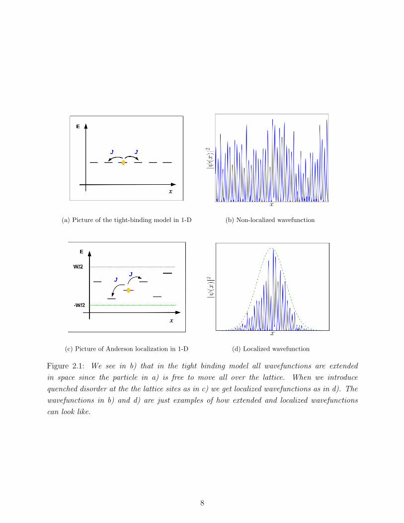
Figure 2.1: We see in b) that in the tight binding model all wavefunctions are extended

in space since the particle in a) is free to move all over the lattice. When we introduce

quenched disorder at the the lattice sites as in c) we get localized wavefunctions as in d). The

wavefunctions in b) and d) are just examples of how extended and localized wavefunctions

can look like.

8

Where ~k is the wavenumber and ~ri is the location of a particle at site i with wavefunction

|i〉. Such a system is known to generally be conductive. In the opposite limit of finite W

and J = 0, the eigenstates are the |i〉’s with eigenenergies hi’s, i.e. all the eigenstates are

localized on the individual lattice sites and the system is thus insulating. After considering

the two limits of J/W it is interesting to look at where the transition between the localized

system at J/W = ∞ and the metallic system at J/W = 0 is. More concretely we wish to

know if there is a transition at a finite value of J/W . Anderson showed perturbatively that

in three dimensions the transition will indeed occur at finite J/W , i.e. the conductivity will

remain zero for small but finite J/W . He performed the perturbation theory in the localized

limit, treating the hopping as the perturbation. This is usually referred to as the locator

expansion.

To the lowest order in J/W the perturbed eigenstates are

|ψA〉 = |i〉+∑j

J

hi − hj|j〉 (2.4)

Since hi’s are random we can only make probabilistic statements about whether or not the

second term is small, which we need in order for the perturbation theory to be valid. The

typical value of hi−hj is W/2, which means that the typical smallest value of hi−hj for any

given i is W/2z, where z is the coordination number of the lattice, i.e. the number of nearest

neighbors. Therefore we naively expect the perturbation theory to be valid if 2Jz/W < 1.

This conclusion turns out to be correct, although the argument above is clearly far from

foolproof. There is always a possibility for hi − hj being small, and to higher order in

perturbation theory we will eventually with certainty encounter sites where hi is very close

to hj. We would need to perform a careful probabilistic analysis of the disorder in order to

make any conclusions regarding whether or not such resonances will hurt the perturbation

theory. Anderson set up the perturbation theory and showed that localization persists with

probability one in the thermodynamic limit. However, he was also not completely rigorous

in proving that the states nearby in energy do not harm the perturbation theory, and it was

not until later that this was rigorously proven by Frohlich and Spencer [37].

Thus for small J/W the states of three dimensional system are localized and its

wavefunction ψi(~r) has an envelope which goes as

ψi(~r) ∼ e−|~r−~ri|ξ (2.5)

where ξ is the localization length and ~ri the localization center. Conversely a non-localized

state has an extended wavefunction which is spread out over the entirety of space like ψi(~r) ∼1/√V , where V is the volume of space. It is widely believed that extended and localized

wavefunctions cannot co-exist in the same energy range. Therefore they split into bands

which are separated by so-called mobility edges Em. As we have argued above, in three

dimensions there is a transition from extended states to exponentially localized states. This

9

transition can happen through special “critical states” at the mobility edge which displays

power-law localization.

2.2 Scaling Theory to Anderson Localization

Apart from Anderson’s perturbative study, there are many other ways to approach the

problem of localization. The so-called “Gang of Four” consisting of Abrahams, Anderson,

Licciardello, and Ramakrishnan [17] were some of the first to consider a scaling theory of

Anderson localization. We review some of their results in the following.

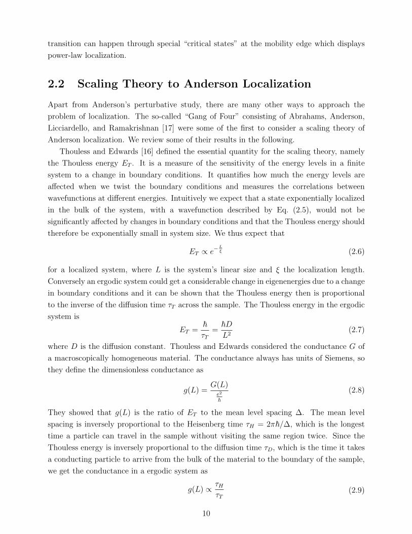
Thouless and Edwards [16] defined the essential quantity for the scaling theory, namely

the Thouless energy ET . It is a measure of the sensitivity of the energy levels in a finite

system to a change in boundary conditions. It quantifies how much the energy levels are

affected when we twist the boundary conditions and measures the correlations between

wavefunctions at different energies. Intuitively we expect that a state exponentially localized

in the bulk of the system, with a wavefunction described by Eq. (2.5), would not be

significantly affected by changes in boundary conditions and that the Thouless energy should

therefore be exponentially small in system size. We thus expect that

ET ∝ e−Lξ (2.6)

for a localized system, where L is the system’s linear size and ξ the localization length.

Conversely an ergodic system could get a considerable change in eigenenergies due to a change

in boundary conditions and it can be shown that the Thouless energy then is proportional

to the inverse of the diffusion time τT across the sample. The Thouless energy in the ergodic

system is

ET =~τT

=~DL2

(2.7)

where D is the diffusion constant. Thouless and Edwards considered the conductance G of

a macroscopically homogeneous material. The conductance always has units of Siemens, so

they define the dimensionless conductance as

g(L) =G(L)e2

~

(2.8)

They showed that g(L) is the ratio of ET to the mean level spacing ∆. The mean level

spacing is inversely proportional to the Heisenberg time τH = 2π~/∆, which is the longest

time a particle can travel in the sample without visiting the same region twice. Since the

Thouless energy is inversely proportional to the diffusion time τD, which is the time it takes

a conducting particle to arrive from the bulk of the material to the boundary of the sample,

we get the conductance in a ergodic system as

g(L) ∝ τHτT

(2.9)

10

This leads us to an intuitive assumption for when the system fails to be ergodic in terms of

g(L). When the Thouless time is larger than the Heisenberg time, particles will not reach

the boundary from the bulk. Thus, we expect that for g < 1, i.e. when the Thouless energy

is much smaller than the level spacing, the system is not ergodic. Conversely when g > 1

the particles will eventually travel all around the system, and the system is ergodic. The

transition between the Anderson localized and non-localized phases is thus expected to occur

when ET and ∆ are of the same order of magnitude.

The great insight of the “Gang of Four” which lead to the scaling theory of Anderson

localization was that g(L) should be the only relevant parameter for determining the

conductive properties of the system, and that it depends on L in an universal manner.

Having recognized g(L) as the universal variable, we consider putting nd identical blocks of

length L together into a hypercube of linear dimension nL. Then the conductance of the

hypercube g(nL) should only depend on the conductance of the smaller system g(L). That

is, we have

g(nL) = h(n, g(L)) (2.10)

That this equation should hold was an educated guess known as one-parameter scaling, and

it is essentially an application of the renormalization group to the Anderson localization

problem. We wish to have the scaling equation Eq. (2.10) on a continuous form, so we

consider the case where n = 1 + dn, which gives us

g((1 + dn)L) = h((1 + dn), g(L))

= g(L) + g(L)β(g(L))dn

⇒ β(g(L)) =L

g(L)

g(L+ Ldn)− g(L)

Ldn

(2.11)

Where β(g(L)) is a scaling function. We take the limit dn→ 0 and get

d log(g)

d log(L)= β(g(L)) (2.12)

Which is the renormalization group equation governing g(L). The physical significance of the

scaling function β(g) is that if we start out with a system of linear size L and conductance

g(L) for which β(g) < 0, then the conductance will decrease upon enlarging the system, and

conversely the conductance will increase if β(g) > 0. That is, the β-function encodes the

transport properties of the system in the thermodynamic limit. We do not know exactly how

this β-function looks like, but we can easily find its asymptotic behavior in the limits of very

large and very small conductance.

We now consider the limit of weak disorder, which we expect leads to large conductance

g 1. In this regime we expect the G(L) to be given by Ohm’s law

G(L) = σL

A⇒ g(L) = σ0L

d−2 (2.13)

11

Figure 2.2: The scaling plot deduced by the “Gang of Four”. Figure from [17].

where σ0 proportional to the conductivity. Inserting this into the renormalization group

equation Eq. (2.12) to obtain

limg→∞

β(g) = d− 2 (2.14)

We have seen that for strong disorder all wavefunctions are exponentially localized, therefore

the conductance should also be exponentially small in system size. We therefore assume the

scaling g(L) = exp(−L/ξ), which means that

limg→0

β(g) = log( ggc

)(2.15)

Where gC is the critical value of conductance. Knowing the asymptotic form of the β(g) for

very strong and very weak disorder, we can use the simplest interpolation between the two

limits to arrive at the famous scaling plot from the “Gang of Four” paper in Fig. 2.2. We see

here that in one and two† dimensions all states are localized for arbitrarily small disorder,

but in three dimensions we have a mobility edge. In three dimensions there is a transition

for at the critical value of conductance gC , which we above argued should be gC ≈ 1.

It is not obvious that Eq. (2.10) should hold, but the same results as we have presented

in this section have been verified through the use of a renormalization group approach to a

version of the non-linear σ-model. This is a field theory which was first proposed by Wegner

[18] and later Efetov[21] pioneered a supersymmetric version of the σ-model, which was used

†We note that in two dimensions the picture is actually a bit more nuanced, and there can be delocalized

states depending on the symmetry class of the Hamiltonian.

12

to verify some of the scaling theory’s results for Anderson localization [19, 20].

2.3 Localization with Interactions

After understanding single-particle Anderson localization reasonably well, we wish to consider

what happens to an Anderson localization when we turn on interactions.

The Anderson model is a rather unrealistic model for any conceivable physical system, as

there will generally be some coupling to the external world and particles will interact with

each other. We will here consider what happens when we try to make the Anderson model a

bit more general. We first let the system interact with phonons, i.e. couple it to a heat bath,

and then we look at a closed system with inter-particle interactions.

2.3.1 Coupling to Heat Bath

It is believed that if we turn on, even a very week, coupling to a heat bath with a continuous

spectrum the conductivity will become finite.

We provide a crude “derivation” of the conductivity in the the variable-range hopping

model, as first discussed by Mott [22]. The model describes conduction in a d-dimensional

system where all charge carriers are localized, and which is weakly coupled to a heat bath.

We consider a system of fermions at low temperatures with strong quenched disorder and

a well-defined Fermi-level, in which all the states near the Fermi-level is occupied. Two

adjacent states in energy are generally localized far apart in space. If the system is coupled

to a heat bath there are delocalized phonons with energies arbitrarily close to zero, and the

fermions can then exchange energy with the phonons of the heat bath and hop over long

distances. This happens because there will always be a phonon of the correct energy to

match the energy difference between two single-particle states, and the phonons can thus

excite fermions above the Fermi-level and induce conduction.

We consider tunneling between states with localization centers separated by R and with

energies E1 and E2 lying above and below the Fermi-level respectively. The probability

for tunneling decays as exp(−2R/ξ) where ξ is the localization length. The probability to

produce excitations of order E1−E2 in the heat bath goes as exp((E1−E2)β). Which leads

us to assume that the conductivity to leading order is

σ(β) ∼ e−2Rξ−(E1−E2)β (2.16)

13

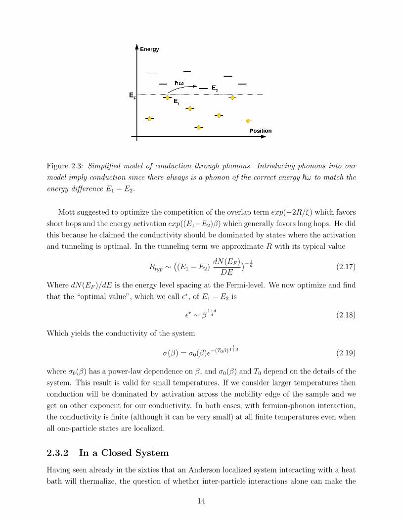
Figure 2.3: Simplified model of conduction through phonons. Introducing phonons into our

model imply conduction since there always is a phonon of the correct energy ~ω to match the

energy difference E1 − E2.

Mott suggested to optimize the competition of the overlap term exp(−2R/ξ) which favors

short hops and the energy activation exp((E1−E2)β) which generally favors long hops. He did

this because he claimed the conductivity should be dominated by states where the activation

and tunneling is optimal. In the tunneling term we approximate R with its typical value

Rtyp ∼((E1 − E2)

dN(EF )

DE

)− 1d (2.17)

Where dN(EF )/dE is the energy level spacing at the Fermi-level. We now optimize and find

that the “optimal value”, which we call ε∗, of E1 − E2 is

ε∗ ∼ β1+dd (2.18)

Which yields the conductivity of the system

σ(β) = σ0(β)e−(T0β)1

1+d(2.19)

where σ0(β) has a power-law dependence on β, and σ0(β) and T0 depend on the details of the

system. This result is valid for small temperatures. If we consider larger temperatures then

conduction will be dominated by activation across the mobility edge of the sample and we

get an other exponent for our conductivity. In both cases, with fermion-phonon interaction,

the conductivity is finite (although it can be very small) at all finite temperatures even when

all one-particle states are localized.

2.3.2 In a Closed System

Having seen already in the sixties that an Anderson localized system interacting with a heat

bath will thermalize, the question of whether inter-particle interactions alone can make the

14

system thermal was timely. However it took almost 50 years from Anderson’s original paper

until Basko et al. [2] were able to answer this question rigorously†. Their calculations are

rather lengthy so we will just mention their results and which sorts of systems it applies to.

We assume we have a highly disordered system, in which all the single-particle states are

Anderson localized, and then let the particles interact with each other with an interaction

strength Jint. We start by considering the two limits of Jint. If Jint = 0 we retain Anderson’s

model and the system is obviously localized and conversly if Jint is very large we intuitively

expect the model to be non-localized since the disorder in this case is insignificant in

comparison with the strong interaction. Therefore there should be some crossover from the

localized to the ergodic phase, and the natural question to ask is if this crossover happens

at finite Jint. It was this question Basko et al. tried to answer as they considered a closed

system at energy densities corresponding to low, but finite, temperatures. They considered

the Hamiltonian

H =∑i

εic†ici +

∑ijkl

Jijkl c†ic†jckcl (2.20)

where c†i creates a single particle state which is Anderson localized with localization center

~ri, localization length ξ and energy εi. They performed perturbation theory in the low

temperature-limit of weakly interacting fermions, in a similar manner to Anderson’s locator

expansion. The perturbation theory is performed in the basis of occupied single-particle

eigenstates

|φα〉 = |nα0nα1 . . . nαi〉 (2.21)

Where nαi are the occupation numbers of the localized eigenstates. The occupation numbers

completely determines |φα〉, which is a state in fermionic Fock space. The interactions are

short range and the matrix elements Jijkl are constrained in both in space and energy, and

the interaction term Jijkl is thus treated as a perturbation. It plays a similar role as the

hopping between sites did in Anderson localization, and the full MBL problem looks like

the Anderson problem on a hypercubic lattice in N dimensions, where each site is a basis

state in Fock space and Jijkl gives rise to “hopping” in Fock space. The interaction mixes

the single-particle states that are close in Fock space, but assuming Jijkl h the mixing is

suppressed with probability O(J/h).

Basko et al. showed to all powers in perturbation theory that, for small enough Jijkl,

localization in Fock space persists up to a finite energy density which is extensive in the system

size, and conductivity can be zero at finite temperatures. This was proof that Anderson

localization can occur in an interacting system and answers the question posed by Anderson;

disorder can indeed prohibit a closed system from thermalizing.

†Actually Mirlin et al. [3] showed this about a year earlier. However this paper has not received as much

attention as the paper by Basko et al. [?]

15

Chapter 3

Random Matrix Theory

We will in this chapter review “random matrix theory” (RMT), which will be crucial when

discussing quantum thermalization later. RMT has had tremendous success in many areas

of physics and it was first brought to the fore by Wigner [23, 24] and Dyson [25], who

developed the theory in order to explain the spectra of complex nuclei. Wigner realized

that it would be hopeless to try to calculate the exact energy eigenvalues of huge quantum

systems, such as heavy nuclei, instead he considered focusing on their statistical properties.

Wigner postulated that in an energy range far from the ground state, the Hamiltonian of

the nuclei should not, from a statistical point of view, differ significantly from an ensemble

of random matrices. He demanded that the ensemble supports unitary quantum evolution,

i.e. its matrices must be hermitian, that all symmetries must be taken into account and that

no additional information is encoded into the ensemble, in particular there should be no

privileged direction of Hilbert space. When these constrains were met, Wigner claimed that

the exact details of the distributions do not matter much.

This idea might indeed seem quite counter-intuitive, but Wigner was able to rather

accurately predict the spacing between the lines in the spectra of heavy nuclei. If we

look at a small energy-window where the density of states is constant, the Hamiltonian

of many large, complex systems will, in a non fine-tuned basis, appear much like a random

matrix. Therefore it does indeed make sense that we may gain insights into complex physical

systems by studying random matrices subject to the same symmetries as those of the systems’

Hamiltonian. Wigner and Dyson considered approximating the Hamiltonian by a Gaussian

ensemble of finite large N×N-matricesH which have the probability density of its independent

elements as

P (Hnm) ∝ e−ζtrH2

2a2 (3.1)

Where the factor ζ depends on the ensemble and a sets the overall energy scale. In other

words the matrix elements are essentially independent Gaussian random variables, but they

have to comply with the symmetries of the Hamiltonian. The matrix elements are real in

the orthogonal, complex in the unitary or real quaternions in the symplectic ensemble. The

16

Gaussian orthogonal ensemble (GOE) contains real, symmetric matrices and corresponds to

systems with time-reversal symmetry and it is this case which will interest us in the following.

This is mainly because the model we will be studying later is time-reversal invariant. However,

it is also of particular interest to see that equilibrium statistical mechanics, with its arrow

of time, can emerge in time-reversal invariant systems. That is, how a system which is

microscopically time-reversal invariant can break the the invariance on a macroscopic level.

3.1 Wigner Surmise

We will now derive a probability distribution function (PDF) for the spacings of the energy

levels of GOE systems. We will use the 2×2 case to deduce the so-called Wigner Surmise.

We consider the general real, symmetric matrix

H2×2 =

(ε1

V√2

V√2

ε2

)(3.2)

with eigenvalues

λ1/2 =ε1 + ε2

2± 1

2

√(ε1 − ε2)2 + 2V 2 (3.3)

Where the factor of 1/√

2 is inserted since it leaves the Hamiltonian invariant under basis

rotations. Since ε1, ε2, and V are independent variables drawn from a Gaussian distribution,

which we for simplicity assume to have zero mean and unit variance, we can easily find the

the statistics of the separation between the energy levels

P1(λ1 − λ2 = ω) =1

(2π)32

∫dε1dε2dV δ(ω −

√(ε1 − ε1)2 + 2V 2)e−

ε21+ε22+V 2

2

We here change variables to ε2 = ε1 +√

2η, which gives us a Gaussian integral in E1, which

is trivial to integrate. We then get

P (ω) =1

2π

∫dη dV δ(

√2η2 + 2V 2 − ω)e−

η2+V 2

2

=1

2π

∫ 2π

0

dθ

∫ ∞o

dr r δ(√

2r − ω)e−r2

2

=ω

2e−

πω2

4

(3.5)

Where we changed to spherical coordinates η = r cos(θ) and V = r sin(θ) before integrating.

We have deduced the distribution function for level separation for the Gaussian Orthogonal

Ensemble in two dimensions. This is the celebrated Wigner Surmise with which Wigner was

able to explain statistical properties of the spectra of complex nuclei.

Off course such nuclei contains much more than two degrees of freedom, but Wigner

made a leap of faith and assumed the two-dimensional result also to be approximately valid

17

for systems with more degrees of freedom. In fact, the two-point level spacing function

has, some time after Wigner, been solved exactly in N dimensions and it turns out that

Wigner’s Surmise is indeed a very good approximation for the probability distribution of

level spacings as N → ∞. We can easily verify this numerically by generating many large

GOE matrices, which we then diagonalize and estimate the level spacing and average over

many realizations of such matrices to estimate the PDF numerically.

3.2 Probability Distribution for the Eigenvalues

Having derived the PDF for the two energy levels of two-dimensional GOE-matrices, we

generalize this to N dimensions in the following. To make predictions about the spectra

Ek of systems of random matrices belonging to GOE, we need to deduce the statistics

of the eigenvalues of H. Whereas the matrix elements are roughly uncorrelated random

numbers, we will see that the eigenvalues are highly correlated. We now wish to find the joint

probability distribution P (Ek) for the N eigenvalues. We write the eigenvalue equation as

H = V EV T ⇐⇒ Hnm =∑i

Eivnivmi (3.6)

Where E is a N × N diagonal matrix of eigenvalues and V a N × N orthogonal matrix

whose columns consist of the eigenvectors of H, which is a real, symmetric matrix and

has N(N + 1)/2 independent variables. The matrix of eigenvectors V must satisfy N(N −1)/2 orthogonality constraint and can therefore be determined by N(N − 1)/2 independent

parameters which we denote β1, β2 . . . βN(N−1)/2. Since we wish to obtain the probability

distribution function of the eigenvalues, we make a change of variables from Hnm to Ek and

βj, which we substitute into P (H) defined in Eq. (3.1). We can use the orthogonality of the

eigenvectors to see that

trH2 =∑n

∑kl

EkElvnkvmkvolvnl =∑k

E2k . (3.7)

Due to the fact that the probability is conserved and using Eq. (3.7) we have

P (E)dE = P (H)dH = Ce−ζ∑k E

2kdH (3.8)

where

dH = dH11dH12 . . . dHNN ∧ dE = dE1 . . . dENdβ1 . . . dβN(N−1)/2 (3.9)

We will now make the coordinate transformation dH = JdE , which leaves us with

P (E)dE ∝ Je−ζ∑k E

2kdE (3.10)

18

Then all that remains is to calculate the Jacobian J(E1, . . . , EN , β1, . . . , βN(N−1)/2) for this

transformation. The Jacobian is

J =

∣∣∣∣∣ ∂(H11, H12 . . . HNN)

∂(E1 . . . EN , β1 . . . βN(N−1)/2)

∣∣∣∣∣ (3.11)

Where tensor notation is implied. We see from Eq. (3.6) that Hnm is a linear function

of the eigenvalues which implies that ∂Hnm/∂βi is linear in eigenvalues as well, and that

∂Hnm/∂Ei is independent of the eigenvalues. We thus see that J must be a polynomial of

degree N(N − 1)/2 in each of the eigenvalues.

If two eigenvalues are equal their corresponding eigenvectors are not uniquely determined

and the inverse transformation of Eq. (3.6) is not properly defined, so J must therefore vanish

when En = Em for all n and m. This may also be seen from the fact that determinants

with duplicate columns always evaluates to zero. J thus contains every possible distinct

combinations of |En − Em| as a factor. There exists N(N − 1)/2 such combinations and

since J is a N(N − 1)/2’th degree polynomial in eigenvalues, all of J ’s dependence on the

eigenvalues is accounted for and we have

J = Πn<m|En − Em|f(β1, . . . βN(N−1)/2) (3.12)

We do not care about the dependence on βi’s since we only wish to know the statistics of

the eigenvalues Ek, therefore we simply assume all of the βj-dependence to be contained

in some function f(β1, . . . βN(N−1)/2). Now we can use this expression for the Jacobian and

we get the following PDF

P (E) ∝ e−ζ∑k E

2kΠn<m|En − Em|f(β1, . . . βN(N−1)/2) (3.13)

We integrate out the dependence on the β’s, this yields some normalizing constant which

we disregard at this stage. We can always normalize our PDF at some later time. We then

arrive at the joint probability distribution for the eigenvalues

PGOE(Ek) = C Πn<m|En − Em|e−ζ∑k E

2k (3.14)

We see clearly from Eq. (3.14), that the probability for having degeneracies in the spectrum

is zero and that the probability for finding energy levels very close to each other is small.

This effect is called level repulsion and it is one of of the main characteristics of RMT.

The probability distribution function in Eq. (3.14) should be used to obtain results for

expectation values of correlation functions of the energy levels within the GOE. However

it might get extremely complicated to obtain exact result even for a two-level correlation

function when we are dealing with large systems. We will see an example of the PDF in use

later; when we calculate a three-point correlation function in Appendix B.

19

3.3 Matrix Elements in RMT

The eigenvectors φn = (φn1 , . . . , φnN) of large GOE matrices are given by the following

probability distribution of its components [40, 44]

P (φ1, . . . , φN) ∝ δ(1−

∑k

φ2k

)(3.15)

Where φnk is the k’th component of the n’th eigenvector. This form follows from the

fact that the orthogonal invariance of the GOE implies that the PDF only depends on

the norm√∑

k φ2k and should thus be proportional to the δ-functions. We see from Eq.

(3.3) that the eigenvectors are basically random and uncorrelated unit vectors. Due to

the orthogonality restriction this cannot be completely accurate, but since two uncorrelated

vectors in a large-dimensional space are usually nearly orthogonal we assume that we can

disregard of the orthogonality restrictions between the eigenvectors.

We note that the matrices of GOE can be diagonalized and the eigenvectors form a basis,

in which the matrix is diagonal and GOE gives the statistics of the eigenvalues. The statistical

properties of the eigenvectors given by the PDF in Eq. (3.3) are specified in a fixed basis

for an entire ensemble of random matrices. It thus holds for N → ∞, that the projections

of GOE eigenvectors onto a fixed vector in Hilbert space have a Gaussian distribution with

zero mean and unit variance [45].

We now move on to study matrix elements of hermitian operators within the framework

of RMT. We consider the some given local operator

A =∑k

Ak|k〉〈k| (3.16)

where |k〉 are the eigenvectors of some given GOE-matrix. We have the matrix elements

Anm = 〈n|A|m〉 =∑k

Ak〈n|k〉〈k|m〉 =∑k

Ak(φnk)∗(φmk ) (3.17)

Using that the eigenvectors are essentially random orthogonal unit vectors we see that to

leading order in 1/N , where N is the dimension of the matrices, we have

〈φnkφml 〉 ≈1

Nδklδnm (3.18)

where 〈φnkφml 〉 is an average over |n〉 and |m〉. We can now utilize Eq. (3.18) to give us the

expectation values of matrix elements

〈Anm〉 ≈δnmN

∑k

Ak = δnmA (3.19)

Where we see that the expectation values of the off-diagonal elements are zero and all of

the diagonal elements have the average value A ≡∑

k Ak/N as their expectation value. We

move on to consider the fluctuations. We have

〈A2nm〉 − 〈Anm〉2 =

∑i,j

AiAj〈φni φmi φnj φmj 〉 −∑i,j

AiAj〈φni φmi 〉〈φnj φmj 〉 (3.20)

20

To evaluate the average of the fluctuations we will need to use Isserli’s or Wick’s Therem

[27], which in our notation and in four dimensions states that

〈φni φmi φnj φmj 〉 = 〈φni φmi 〉〈φnj φmj 〉+ 〈φmi φnj 〉〈φni φmj 〉+ 〈φni φnj 〉〈φmi φmj 〉 (3.21)

We will consider the diagonal and off-diagonal elements separately. Using Eq. (3.21) we get

the following for the fluctuations of the diagonal elements

〈A2mm〉 − 〈Amm〉2 =

∑i

A2i (〈φmi 〉4 − 〈(φmi )2〉2)

= 2∑i

A2i 〈(φmi )2〉2

=2

NA2

(3.22)

Whereas for the off-diagonal elements we have

〈A2nm〉 − 〈Anm〉2 =

∑k

A2k〈(φmk )2(φnk)2〉 =

1

NA2 (3.23)

We can now approximate the matrix elements to leading order in 1/N as

Anm ≈ Aδnm +

√A2

NRnm (3.24)

where Rnm is a random variable with zero mean and unit variance on the off-diagonal elements

and the diagonal elements have variance two. It is simple to see that the ansatz in Eq. (3.24)

gives the correct fluctuations and average of matrix elements within the GOE. We averaged

over the random Hamiltonian ensemble to arrive at the above expression but when N is large

the fluctuations should be very small, and therefore the expression should be applicable also

to single Hamiltonians.

The question concerning which systems RMT generally applies to still remains. RMT

has found applications in nuclear physics, quantum gravity, quantum chromodynamics, the

fractional quantum Hall effect and many other places.

In the same way as classical thermodynamics can describe a huge variety of different

microscopical systems at a macroscopic level, also RMT can arise from many different

microscopical systems, and RMT is insensitive to the interactions at a microscopical level.

There exists many other random matrix ensembles and one of them we will see in Chap. 6,

namely the Wishart matrix. This is rather similar to the GOE, but it has a slightly different

PDF for its matrix elements.

As an aside, it is worth mentioning that there exists an interesting connection between the

level statistics in RMT and the statistics of non-trivial zeros of the Riemann zeta function.

The Riemann zeta function can be defined as

ζ(s) =∞∑k=1

1

ks=∏p∈P

1

1− p−s(3.25)

21

Where P contains all primes and ζ(s) is defined by Eq. (3.25) for <s > 1 and elsewhere

through analytic continuation. It has been conjectured that the Riemann zeta function

should have all its non-trivial zeros lying on the line s = 1/2 + iEk with Ek ∈ R, this is the

infamous Riemann hypothesis. It has also been shown numerically for about a billion zeros

that the Ek’s fluctuate like the eigenvalues of a unitary Gaussian matrix. This hints toward

a profound connection between prime numbers and RMT, which as we will see in Chap. 4,

lies at the core of quantum chaos and thermalization.

22

Chapter 4

Chaos & Thermalization

In this section we will consider the statistical mechanics of closed quantum systems. If

such systems thermalize, they should approach an equilibrium which is described by the

microcanonical ensemble. It is however not always the case that a closed system is properly

described by the microcanonical distribution, and we want to consider which conditions need

to be satisfied in order for closed quantum systems to be thermal.

There are two common approaches to justify why the rules of statistical mechanics work.

The first is to couple the system to a heat bath with certain properties, with which the system

can exchange energy, particles etc, and whose heat capacity is unaffected upon coming in

contact with the system. This is not the approach we are going to take since it seems in some

way to be rather heuristic and only pushes the problem back one level and would force us to

justify why the heat bath has its thermal properties. Furthermore it does not seem sound to

justify the inherent properties of a closed system by coupling it to an external reservoir.

The other approach is to consider the system in isolation and make some assumption of

ergodicity and mixing, i.e. assuming that the dynamics of the system is in some way chaotic.

It is then possible to derive the thermodynamic distributions. Although completely isolated

quantum systems are not really feasible experimentally, there has recently been made progress

in approximating isolated many-body quantum systems [28], and it is this approach we will

follow.

We thus have to look at what it means for a system to be ergodic and chaotic. We

therefore start by considering chaos, first for classical systems and then for quantum systems,

and thereafter look at how this is related to quantum thermalization.

4.1 Classical Chaos & Integrability

Classically chaotic systems are generally governed by non-linear equations and chaos is

usually defined as an exponential sensitivity of the phase-space trajectories to arbitrary

small perturbations of the initial conditions. Chaos is often quantified through Lyapunov

23

exponents λ, which for chaotic systems show how the difference in phase space trajectories

δZ(t) evolves in time from the initial separation δZ(0).

|δZ(t)| ≈ eλt|δZ(0)| (4.1)

There are classes of systems which are not chaotic and have phase-space trajectories whose

separation cannot be described by Lyapunov exponents, and these systems are called

integrable. Textbook examples of classical chaotic and integrable systems are systems of

one particle moving in a Bunimovich and a circular stadium respectively, as seen in Fig. 4.1.

In the circular cavity the particle would not change its phase space trajectory drastically

if we changed its initial conditions slightly. That is, two trajectories which at one time

are close to each other will after an arbitrarily long time still lie close to each other in the

non-chaotic circular stadium. In the chaotic Bunimovich stadium, two trajectories which

initially lie close together, would lie arbitrarily far apart from each other after a long time.

Chaotic systems are generally ergodic, which means that they with time will cover their

entire available phase space †. A particle in the chaotic Bunimovich stadium will after a

while have had explored all of its available phase-space, whereas in the circular billiards this

is clearly not the case.

Figure 4.1: Trajectories of particle in a cavity. a) Circular stadium with integrable dynamics.

b) Bunimovich stadium with chaotic dynamics. Figure from Scholarpedia [32]

We will now to formalize the notion of integrability. Assume we have an Hamiltonian

H(p, q) with the canonical coordinates q = q1, ..., qN and p = p1, ..., pN. We further

assume that the system have some functionally independent conserved quantities K =

K1, ..., Kj in involution (meaning they have vanishing Poisson brackets between each other).

The conserved quantities are represented by constants of motion with vanishing Poisson

brackets with the Hamiltonian. That is, we have

d

dtKj = Kj, H = 0 ∧ Kj, Ki = 0 (4.2)

†There are some nuanced differences between chaos and ergodicity, depending on how we define them.

We will simply assume that chaotic systems are ergodic, which is indeed usually the case.

24

For all the Kj’s, where the standard Poisson brackets are defined as

f, g =N∑j=1

∂f

∂pj

∂g

∂qj− ∂g

∂pj

∂f

∂qj(4.3)

A system which is Liouville integrable is defined as a system governed by Hamiltonian H(p, q)

defined on IR2N with N or more independent constants of motion in involution.

For Liouville integrable systems there thus exists a canonical transformation (p, q) →(K,Θ) from the momentum and position variables to the so-called action-angle variables

which yields H(p, q) = H(K). The equations of motion are now trivial to solve

Kj(t) = Kj(0) ∧ Θj(t) = Ωjt+ Θj(0) (4.4)

We know that the trajectories in phase space lie on surfaces corresponding to the constants

of motion. For a Liouville integrable system the trajectories are thus restricted to lie on a

N -dimensional tori, and the dynamics is not chaotic.

When we generalize the above to many-particle systems we usually consider systems with

an extensive number of conserved quantities integrable. As an example, a high dimensional

system of many non-interacting particles would not be considered chaotic in this sense, even if

each particle is chaotic in the part of phase-space associated with its own degrees of freedom,

since the energy of each particle is separately conserved.

4.2 Quantum Chaology

Knowing that chaotic systems are governed by non-linear equations and have exponential

sensitivity to initial conditions, quantum chaos is something of a misnomer. Closed quantum

systems do not have exponential sensitivity to initial conditions† and are governed by the

linear Schrodinger equation, in other words, closed quantum systems are never actually

chaotic.

For these reasons Micheal Berry suggested the term “quantum chaology”, as a better

word to use to describe unpredictable quantum behavior. Berry defined quantum chaology

[33] as

“The study of semi-classical, but non-classical, phenomena characteristic of systems

whose classical counterparts exhibit chaos.”

†Furthermore it is not completely clear how to consider the divergence of initially small phase space

separation, since the uncertainty principle does not allow us to determine positions in phase space sharply

within regions smaller than ~

25

Although chaos theory and quantum mechanics are two of the most successful theories of

the 20th century, the interplay between these theories is generally not known. Due to Niels

Bohr’s correspondence principle we know that classical mechanics is reached in the limit

of large quantum numbers, and at large enough energies the predictions from classical and

quantum mechanics does indeed coincide. The Kolmogorov–Arnold–Moser theorem provides

a link between classical mechanics and classical chaos, as it describes how integrable systems

behave under small non-linear perturbation.

Whereas the connections between classical mechanics and quantum mechanics and

classical mechanics and classical chaos are both fairly well understood, it is not generally

known how to reach the non-linear dynamics of classical chaos as a limit of quantum

mechanics. It is not straightforward to see how the extreme irregularity of classical chaos can

arise from the smooth and wavelike nature of phenomenon in the quantum world. It appears

we need novel way of telling which quantum systems are “chaotic” and conversely which

are not. The main objective of quantum chaology is to identify characteristic properties of

quantum systems which, in the semi-classical limit, reflect the integrable or chaotic features

of the corresponding classical dynamics.

One of the hallmarks of quantum mechanics is its quantized energy levels, as opposed to

classical mechanics where energy is continuous. It seems that the first place to look for a way

to distinguish quantum chaotic from non-chaotic systems, is in the spectra of the systems.

However it has also been shown to be a remarkable connection between the wavefunctions

of chaotic systems in the semi-classical limit and classical chaos. A lot has been conjectured

about systems within quantum chaology. We will discuss some of these conjectures in the

following.

4.2.1 Level Spacings of Chaotic and Integrable System

It appears that quantum chaos does not make itself felt at any particular energy level, however

its presence can be seen in the spectrum of energy levels. It has been hypothesized that we can

distinguish between chaotic and non-chaotic quantum systems by looking at the distributions

of energy levels. We present two conjectures which say something about how to recognize

quantum chaotic and non-chaotic behavior.

BGS conjecture

Bohigas, Gionnoni and Schmit [30] conjectured that quantum chaotic systems should have

energy levels which follow RMT statistics. The types of systems for which the conjecture

should apply are simple quantum systems with a well defined classical limit.

”Spectra of time reversal-invariant systems whose classical analogs are chaotic show the

same fluctuation properties as predicted by GOE.”

26

For system without time-reversal symmetry, GUE replaces GOE. There has been a few

attempts to prove the BGS conjecture, but they all have fallen short. Ones confidence in

its applicability stems from that it has been verified numerically on a vast number of simple

systems. Its general validity has now been largely accepted, and it is standard to use it to

statistically address quantum systems which have chaotic behavior. The BGS conjecture

reveals a strong connection between classical chaos and RMT. We have already seen in

Chap. 3 can be used as a tool to describe spectra of quantum systems which are to complex

to solve exactly. Wigner’s work on heavy nuclei could thus be view as an special case of the

BGS conjecture.

Berry-Tabor conjecture

The question of quantum integrability was considered by Berry and Tabor [31]. A simple

example of a non-chaotic system with many degrees of freedom is an array of independent

harmonic oscillators with incommensurable† frequencies. Here the energies will not be

correlated with each other and can be viewed as random numbers. Their distribution should

then be described by Poisson statistics

p(s) =1

δe−

sδ (4.5)

Where s is the spacing between two adjacent energy levels and δ a normalization constant.

Berry and Tabor postulated that this should be a general feature of quantum integrable

systems. The Barry-Tabor conjecture states that for quantum systems whose classical

counterpart is integrable, the energy eigenvalues generically behave like a sequence of random

numbers, i.e. the spectra obey Poisson statistics. There are known examples where this fails,

but then usually as a result of emergent symmetries in the Hamiltonian which lead to extra

degeneracies, resulting in commensurability of the spectra.

Poisson and RMT statistics are very different, in that in the former there is no

level-repulsion. Poisson spectra tends to cluster, as can be readily seen from Fig. 4.2.

†a, b ∈ R are said to be commensurable if a/b ∈ Z

27

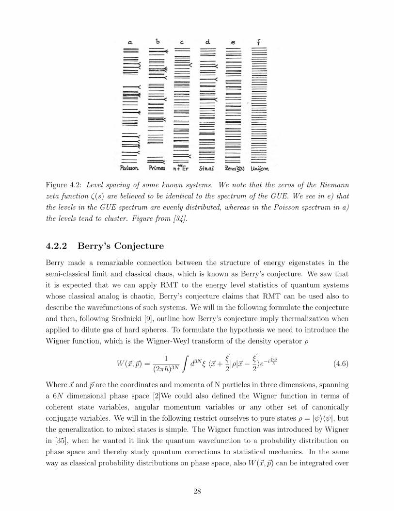
Figure 4.2: Level spacing of some known systems. We note that the zeros of the Riemann

zeta function ζ(s) are believed to be identical to the spectrum of the GUE. We see in e) that

the levels in the GUE spectrum are evenly distributed, whereas in the Poisson spectrum in a)

the levels tend to cluster. Figure from [34].

4.2.2 Berry’s Conjecture

Berry made a remarkable connection between the structure of energy eigenstates in the

semi-classical limit and classical chaos, which is known as Berry’s conjecture. We saw that

it is expected that we can apply RMT to the energy level statistics of quantum systems

whose classical analog is chaotic, Berry’s conjecture claims that RMT can be used also to

describe the wavefunctions of such systems. We will in the following formulate the conjecture

and then, following Srednicki [9], outline how Berry’s conjecture imply thermalization when

applied to dilute gas of hard spheres. To formulate the hypothesis we need to introduce the

Wigner function, which is the Wigner-Weyl transform of the density operator ρ

W (~x, ~p) =1

(2π~)3N

∫d3Nξ 〈~x+

~ξ

2|ρ|~x−

~ξ

2〉e−i

~ξ·~p~ (4.6)

Where ~x and ~p are the coordinates and momenta of N particles in three dimensions, spanning

a 6N dimensional phase space [2]We could also defined the Wigner function in terms of

coherent state variables, angular momentum variables or any other set of canonically

conjugate variables. We will in the following restrict ourselves to pure states ρ = |ψ〉〈ψ|, but

the generalization to mixed states is simple. The Wigner function was introduced by Wigner

in [35], when he wanted it link the quantum wavefunction to a probability distribution on

phase space and thereby study quantum corrections to statistical mechanics. In the same

way as classical probability distributions on phase space, also W (~x, ~p) can be integrated over

28

momentum to give a probability distribution over ~x as∫d3Np W (~x, ~p) = |ψ(~x)|2 (4.7)

It is however not a true probability distribution since it can become negative, and these

regions of negative W (~x, ~p) can be seen as signatures of the presence quantum effects. The

Wigner function is uniquely defined for any state and it plays the role of a quasi-probability

distribution on phase space. The Wigner function can be used to calculate expectation values

of any standard operator A as a phase-space average

〈A〉 =

∫d3Nx d3Np AW (~x, ~p)W (~x, ~p) (4.8)

Where AW (~x, ~p) is the Wigner-Weyl transform of the operator A as defined in Eq. (4.6). The

Wigner-Weyl transform maps the operator onto phase-space, in a way which allows us to take

the phase-space average by integrating over ~x and ~p. Berry’s conjecture states that in the

semi-classical limit of quantum systems whose classical counterpart is chaotic, the Wigner

function of energy eigenstates averaged over a vanishingly small phase space reduces to the

microcanonical distribution. To specify, we consider the following locally averaged Wigner

function

Wn( ~X, ~P ) =1

(2π~)N

∫∆Γ1

dp1dx1 . . .

∫∆ΓN

dpNdxN Wn(~x, ~p) (4.9)

where ∆Γi is a small phase space volume around Xi and Pi and Wn is the Wigner-Weyl

transformation of a pure energy eigenstate ρn = |n〉〈n|. This volume is chosen such that

when we take the classical limit of Planck’s constant going to zero, we have both ∆Γi → 0

and ~/∆Γi → 0 hold. Mathematically we have Berry’s conjecture as

lim~→0

Wn( ~X, ~P ) =δ(E −H( ~X, ~P ))∫

d3NX d3NP δ(E −H( ~X, ~P ))(4.10)

where H( ~X, ~P ) is the systems classical Hamiltonian. In Berry’s words “ψn(~x) are Gaussian

random functions in ~x whose spectrum at ~x are the local averages of their Wigner functions

Wn”. Berry also postulated that the energy eigenfunctions of systems whose classical

counterpart is integrable would have a very different structure.

Application of Berry’s Conjecture

We now follow Srednicki [9] and consider a system of a dilute gas consisting of identical hard

spheres and we will show that the validity of Berry’s conjecture implies that the system will

be thermal. It is well known that the classical distribution of momenta for the individual

particles of such a system will follow the Maxwell-Boltzmann distribution at a temperature

T

fMB(~p1, T ) =e− ~p1

2

2mkBT

(2πmkBT )32

(4.11)

29

where m is the mass of the particles and kB the Boltzmann constant. This is a quantum

system which has a chaotic classical counterpart, since there is no extensive amount of

constants of motion. Thus it is reasonable to assume the validity of Berry’s conjecture

and we will show that this assumption is enough to “re-derive” the distribution of momenta

fMB(~p1, T ) for the quantum system. Srednicki used that an energy eigenstate corresponding

to a high-energy eigenvalue En can always be chosen to be real and can generally be written

as a superposition of plane waves with momentum ~p 2 = 2mEn.

ψn(~x) = Nn∫d3Np An(~p)δ(~p 2 − 2mEn)e

i~p·~x~ (4.12)

where Nn is a normalization constant and A∗n(~p) = An(−~p). Srednicki introduced the

fictitious “eigenstate ensemble” (EE) of energy eigenstates of the system to average over

instead of Berry’s average over a small phase-space volume. The eigenstate ensemble should

describe the properties of typical energy eigenfunctions and individual eigenfunctions behave

as if they were chosen randomly from the eigenstate ensemble. Berry’s conjecture implies

that in the eigenstate ensemble A(~p) should be a Gaussian random variable that and the

two-point correlation function is given by

〈Am(~p)An(~k)〉EE =δ3N(~p+ ~k)

δ(|~p| 2 − |~k| 2)δnm (4.13)

Where the denominator is needed for proper normalization. We Fourier transform our wave

function

φn(~p) = (2π~)−3N2

∫d3Nx ψn(~x)e

−i~p·~x~

= (2π~)−3N2 Nn

∫d3Nk An(~k)δ(~k 2 − 2mEn) δ3N

V (~k − ~p)(4.14)

Where we have introduced δ3NV (k) = (2π~)

∫Vd3N~x exp(i~p · ~x/~). We consider the thermal

de Broglie wavelength λth = (2π~2/(mkBT ))1/2, which is roughly the average de Broglie

wavelength of the particles of an ideal gas. We assume that the λth < a, where a is the radius

of the particles. We also have that L3 a3N since we assumed a low density gas. This gives

〈φ∗m(~p)φn(~k)〉EE = N 2n(2π~)3Nδmn δ(~p

2 − 2mEn) δ3NV (~k − ~p) (4.15)

From this we can calculate the momentum distribution of particles in the eigenstate ensemble.

We integrate out the dependence of all but one particle to get the probability distribution of

momentum of the single particles

〈φnm(~k1)〉EE ≡∫d3p2 . . . d

3pN 〈φ∗n(~p)φm(~p)〉 = N 2nL

3N

∫ ∫d3p2 . . . d

3pN δ(~p 2 − 2mEn)

(4.16)

30

This should equal the Maxwell-Boltzmann distribution at approximately the temperature

given by the ideal gas law T = 2U/3kBN . To show this we to make use of

IN(q) =

∫dNp δ(~p 2 − q) =

(πq)N2

qΓ(N2

) (4.17)

Where Γ(z) is the gamma-function†. Using this we get that the normalization of φn(p)

demands that N−2n = L3NI3N(2mEn). We use this to rewrite Eq. (4.16) and we arrive at

〈φnm(~p1)〉EE =I3N−3(2mEn − ~p1

2)

I3N(2mEn)=

Γ(

3N2

)Γ(3(N−1)

2

)( 1

2πmEn

) 32

(1− ~p1

2

2mEn

) 3N−52

(4.18)

We now substitute the energy En for the temperature corresponding to the energy given by

the ideal gas law En = 3NkBTn/2. We use that Γ(3N/2)/Γ(3(N − 1)2) quickly approaches

one for large values of N . We are interested in the thermodynamic limit, so we now get

limN→∞

〈φnm(~p1)〉EE =( 1

2πmkbTn

) 32 e− ~p1

2

2mkBTn (4.19)

Which is indeed the Maxwell-Boltzmann distribution of momentum for thermal particles.

Srednicki [9] also showed that the if we assume the wavefunction to be completely

anti-symmetric or completely symmetric, we instead would have gotten the Fermi-Dirac or

Bose-Einstein distribution respectively.

4.3 Eigenstate Thermalization Hypothesis

In classical mechanics we know that chaotic systems which cover their phase spaces

homogeneously will generally thermalize, and have macroscopic properties which are

accurately described by the appropriate thermal ensembles. However there can be no

dynamical chaos in closed quantum system, and we therefore need some other way

of explaining why and when closed quantum systems can be described by equilibrium

statistical mechanics.

The solution seems to be the “igenstate thermalization hypothesis” (ETH), which we

already saw signs of in Berry’s conjecture and Srednicki’s work [9]. In this section we will

motivate, define and discuss the ETH.

4.3.1 Background

We start by outlining what sort of systems we will be considering, and more thoroughly

define our notation and what we mean by thermalization.

†Which for <z > 0 is defined as Γ(z) =∫∞0x−zex dx

31

The System

We assume we have a closed system of many degrees of freedom N described by the

Hamiltonian H such that H|n〉 = En|n〉 determines the eigenenergies and energy eigenstates.

The system is bounded, ensuring discrete eigenenergies, and closed, which means that the

time-evolution is governed by the Schrodinger equation. A general state’s time-evolution can

be written as |ψ(t)〉 =∑

nCne−iEnt|n〉, where we assume 〈ψ(t)|ψ(t)〉 = 1 and from here on

set ~ = 1. We assume that the expectation value of energy in the state we are considering is

extensive

〈E〉 =∑n

|Cn|2En ∼ N (4.20)

Which should be roughly satisfied when interactions are short-range, and we also assume the

state to be excited well above the ground state. The uncertainty in energy is assumed to be

much smaller than the total energy and to be decreasing inversely with the system size

∆ =√〈H2〉 − 〈H〉2 〈E〉 ∼ N−ν〈E〉 (0 < ν ≤ 1) (4.21)

This seems to be a reasonable assumption since many physically interesting systems scale

like this when N is large. Furthermore we assume the spectrum of the Hamiltonian be

non-degenerate, which is the case for most chaotic systems. This is consistent with the BGS

conjecture which assumes RMT to be valid for quantum chaotic systems and non-degeneracy

is indeed a property of RMT-spectra.

We let A be some local operator and Anm = 〈n|A|m〉 its matrix elements in the energy

eigenstate basis. We have the expectation value of A in a general state

〈A(t)〉 = 〈ψ(t)|A|ψ(t)〉 =∑n

|Cn|2Ann +∑n6=m

C∗nCme−i(Em−En)tAnm (4.22)

We define the infinite-time average as

〈A〉 = limt→∞

1

t

∫ t

0

dτ〈A(τ)〉 (4.23)

We note that the long-time average might be insufficient when considering equilibration,

since for large systems the energy levels tend to lie exponentially close, and the equilibration

time might thus be unfeasibly long; possibly even longer than that of the universe’s age. We

circumvent this problem and use the purely mathematical infinite time average. We have the

infinite time average of A in a general state as

〈A〉 =∑n

|Cn|2Ann + i~ limτ→∞

[∑n6=m

C∗nCmAnme−i(Em−En)t − 1

(Em − En)τ

]=∑n

|Cn|2Ann(4.24)

Where we have used that the spectrum is non-degenerate.

32

Thermalization

We will consider thermalization in terms of the local operator A and we know that it the

system comes to thermal equilibrium the 〈A〉 should be close to 〈A〉th most of the time. We

thus define a thermal system as one which fulfills

|〈A〉 − 〈A〉th| → 0 ∧ (〈A〉 − 〈A〉)2 → 0 (4.25)

For most initial states. Where 〈· · · 〉th is the thermal average in the appropriate ensemble

and the arrow means “in the thermodynamic limit”. The thermodynamic limit is taken by

letting number of degrees of freedom go to infinity. More precisely we have

N →∞ ∧ V →∞ ∧ N

V= K (4.26)

Where V the system’s volume and K some constant. In other words, we call a system thermal

if, in the thermodynamic limit, the infinite-time average approaches the ensemble average

and the average fluctuations approach zero. The thermal average might be given by the

micro-canonical ensemble at a given energy E with the quantum statistical average

〈A〉m.c.(E) =1

N∆

∑n:En∈X

Ann (4.27)

Where X = [E−∆m.c., E + ∆m.c.], ∆m.c. the energy width of the microcanonical distribution

and N∆ is the number of states in X. This is the appropriate ensemble for closed systems

with given energy, volume and particle number. For systems at inverse temperature β we

might use the canonical ensemble

〈A〉can(β) =1

Z∑n

Anne−βEn (4.28)

Where Z = tre−βH is the standard partition function. The canonical ensemble should

be used when we have given temperature, particle number and volume, i.e. for systems in

contact with a heat bath. We will in the following switch between the ensembles rather

uncritically. The assumption underlying this is that for a system of very many degrees of

freedom and for most non-pathological operators A, the difference between the prediction of

the canonical ensemble at given β and the microcanonical ensemble at given E is small. The

different ensembles do indeed yield exactly the same averages in the thermodynamic limit.

4.3.2 Eigenstate Thermalization Hypothesis

We will consider what it takes for a closed quantum system to thermalize and put forth the

ETH which should tell us which systems are thermal. For a closed system to be thermal we

need the the following to be satisfied in the thermodynamic limit

〈A〉 =∑n

|Cn|2Ann!

=1

N∆

∑n:En∈X

Ann = 〈A〉m.c.(〈E〉) (4.29)

33

We also need the fluctuations to be small

(〈A〉 − 〈A〉)2 =∑n6=m

|Cn|2|Cm|2|Anm|2!

= 0 (4.30)

We note that whereas the time averaged expectation value is determined by the initial state

through the Cn’s, the microcanonical prediction makes no reference to the initial state as it

is determined completely by 〈E〉, which can be the same for many different initial states.

If the eigenstate expectation values Ann practically do not fluctuate at all between

eigenstates that are close in energy, Eq. (4.29) is satisfied for literally all states which are

sufficiently narrow in energy, i.e. for which ∆ is small. We thus need Ann to be smoothly

varying with n and effectively constant over the relevant small energy window. We know

that both ∆m.c. and ∆ are decreasing with increasing system size, and thus for large systems

we can use that Ann varies very slowly with n to draw it outside the sum. Furthermore this

implies that also energy eigenstates themselves are thermal, i.e. we have Ann = 〈A〉m.c.(En).

This is what we call eigenstates thermalization.

We consider the fluctuations and immediately see that for Eq. (4.30) to be satisfied for all

initial states we need the off-diagonal matrix elements Anm to be small. That is, the system

thermalizes if

|An+1,n+1 − An,n| → 0 ∧ ∀n 6= m |Anm| → 0 (4.31)

We notice a similarity between the form of the eigenstate matrix elements imposed on A

by Eq. (4.31) and the expectation values of operators in the GOE. In the GOE the expectation

values of local operators on matrix form† has the average value of the operator on the diagonal

and the off-diagonal fluctuations are decreasing inversely with the system size. By analogy

with Eq. (4.31) and Eq. (3.24) we now arrive at the ansatz of the ETH as defined by Srednicki

[10].

The ETH Ansatz

The ETH ansatz states that local observables should have matrix elements in the eigenstate

basis whose statistics should be described by

Anm = A(E)δnm + e−S(E)

2 g(E, ω)Rnm (4.32)

We first define all the quantities of the equation; we let E = (En+Em)/2, ω = (En−Em) and

Rnm be a factor which varies erratically in n and m††. Furthermore we demand g(E, ω) and

A(E) to be smooth functions of their arguments, where the former is an envelope function on

top of the fluctuations and the latter can be viewed as a spectral function of A. Without loss

†I.e. the statistical expectation value over an ensemble expressed in a fixed basis.††We assume Rnm to essentially be i.i.d. Gaussian numbers.

34

of generality we assume g(E, ω) to be positive, real and an even function of ω. We demand

that Rnm has zero mean and unit variance, and the hermiticity of A implies that Rnm = R∗mn.

The thermodynamic entropy S(E) at energy E is defined by the density of states as

eS(E) = E∑

n δε(E − En) where the Dirac delta function has been smeared out enough to

ensure monotonicity of S(E). The regularized Dirac delta function could be defined e.g. as

δη(x) =1

π

η

η2 + x2(4.33)

For some small η. The ETH ansatz differs from the RMT prediction only in that the diagonal

elements are not all the same and that the small Gaussian fluctuations of the off-diagonal

elements have an envelope function g(E, ω). The ETH ansatz reduces to the RMT form

if we focus on a very narrow energy range where g(E, ω) is constant. The scale at which

ETH and RMT are equal seems to be given by the Thouless energy ET [39]. That is, if

we only consider energies such that ω < ET it holds that g(E, ω) is approximately constant

and that the ETH ansatz is identical to RMT. The Thouless energy goes to zero in the

thermodynamic limit, which implies that RMT has a limited range of applicability. However

the level spacing decreases faster in L than the Thouless energy and thus there are still a

large number of energy levels in the region where RMT applies. Conversely the ETH ansatz

applies to arbitrary energies, with the possible exception of the edges of the spectrum.

A striking feature of the ETH is that knowledge of a single energy eigenstate is sufficient

to compute thermal averages and any eigenstate in the microcanonical window will do, since

they all give the same average.

We show explicitly in Appendix A that when the matrix elements are well described by

the ETH ansatz, the system is indeed thermal. Although the ETH implies that the system

thermalizes, we do not know if the ETH necessarily must hold for all thermal systems. There

has been some numeric evidence for that thermal quantum systems obey the ETH [36]. It is

however hard to study this thoroughly because the only method of investigation is numerically

costly exact diagonalization. We can therefore only test the ETH for very small systems.

4.4 Quantum Thermalization

We now address some issues of the thermal equilibration process in closed quantum systems.

In classical, thermal systems, most initial out-of-equilibrium states approach thermal

equilibrium as the states are evolved in time. This thermal equilibrium is characterized by

a small amount of parameters corresponding to the extensive conserved quantities such as

temperature, chemical potential etc. Most information about the initial state of the system

gets lost during the time evolution.

We do however know that closed quantum systems are governed by the linear Schrodinger

equation. Thus all information about the initial state must be contained in the system at all

times, since unitary time evolution cannot erase information.

35

In order to take a closer look at this we consider the density operator of the system

ρ(t), which we use to find expectation values as 〈A(t)〉 = trρ(t)A. Naively we might

expect that the system coming to equilibrium, means that the initial states evolve into the

Maxwell-Boltzmann distribution ρ(t)→ exp(−βH)/Z†, but this is not the case. To see why,

we consider ρ(t) in terms of its matrix elements in the eigenstate basis

ρ(t) =∑n

ρnn(0)|n〉〈n|+∑n6=m

ρnm(0)e−i(Em−En)t|m〉〈n| (4.34)

We see that the dynamics is simple and that the time evolution merely makes the

off-diagonal matrix elements precess in the complex plane at a constant rate given by the

energy difference between the eigenstates involved. Generally the full system described by

ρ(t) does therefore not approach exp(−βH)/Z at long times; i.e. the distributions of the

thermodynamic ensembles are not attractors of the dynamics.

We have in Eq. (4.25) considered quantum thermalization in terms of local observables,

and thermalization thus requires that the contributions from the off-diagonal matrix elements

to local observables must vanish at long times. Due to the ETH, all energy eigenstates

implicitly contain thermal states, i.e.

tr|n〉〈n|A

= tr

e−βHZ

A

(4.35)

However we can prepare the system in out-of-equilibrium states by giving the phases in ρ(0)

some special structure.

Thermalization of out-of-equilibrium states thus happens because at long times the

off-diagonal terms in ρ(t) come with effectively random phases and their contribution to

expectation values of local operators cancel. Thus states for which 〈A(0)〉 6= 〈A〉th will

after a long time have dephasing between the off-diagonal contributions and therefore

〈A(t)〉 = 〈A〉th at long times. In other words the thermal properties of out-of-equilibrium

states are hidden by the coherence between the eigenstates, but the time evolution reveals

it through dephasing.

Thus we see a distinction from classical mechanics where the time evolution “creates” a

thermal state, which has forgotten everything about its initial state. A quantum system does

not loose any information about the local properties of its initial state, the information is

merely “hidden” somewhere else in the system. What we mean by “hiding” the information, is

that it is made inaccessible, in the sense that recovering it means measuring global operators.

We started this section with stating that some formulations of quantum statistical

mechanics postulate that the system in question is in contact with an external heat bath.

A viewpoint which we dismissed, largely because we would rather consider truly isolated

systems. However we can think about thermalization of closed quantum systems as the

†Or some other equilibrium distribution.

36

different parts of the system acting as heath baths for each other. We consider a small

subsystem S with density operator ρS(t). The density operator on S does not have simple

dynamics since it is an open system with non-unitary time evolution. We thus define

thermalization as†

limt→∞

ρS(t) = trBe−βH

Z (4.36)

Where B contains all the degrees of freedom which are not in S. Even though ρ(t) does

not approach the Maxwell-Boltzmann distribution, the density matrices of small subsystems

appear as if it does. The system can equilibrate under its own dynamics if its different parts

are able to interact in a way which mimics the interaction to a thermal bath††. Information

is moved around in the system, and this makes all the subsystems come to a thermal

equilibrium described by Eq. (4.36)‡.

†Some care need to be taken when taking the thermodynamic limit; it should be taken simultaneously

with the infinite time limit, since finite size systems cannot equilibrate due to quasi-periodic dynamics and

infinite systems need an infinite amount of time to equilibrate.††We do however note that the S and B are strongly interacting, so contrary to systems which are weakly

coupled to a heat bath, the Hamiltonian appearing in ρS is the full system+bath-Hamiltonian, not just HS .‡We note that the equilibration times could presumably differ between different parts of the system.

37

Chapter 5

Model and Methods

5.1 The Model

We will in the following be working with the isotropic Heisenberg Hamiltonian with random

on-site magnetic fields along the z-direction

H =N∑i=1

Szi hi + J∑<i,j>

~Si · ~Sj (5.1)

Where J is the exchange interaction and the hi’s are random fields. The distribution of hi

have some width W and we choose its probability distribution to be uniform and centered

at zero. We have the standard spin operators Sz = σz/2 in terms of Pauli operators and all

operators are filled out with identity operators to a tensor product of N operators. E.g. for

a four-particle system: Sz2Sz3 = I ⊗ Sz ⊗ Sz ⊗ I. We can rewrite the Hamiltonian in a more

useful form

H =N∑i=1

Szi hi + J∑<i,j>

(Szi Szj + Syi S

yh + Sxi S

xj )

=N∑i=1

Szi hi + J∑<i,j>

Szi Szj +

1

2(S−i S

+j + S+

i S−j )

(5.2)

Where we have used the spin raising and lowering operators S±i = Sxi ± iSyi . We will in

the following assume periodic boundary conditions and work in one dimension, in which the

Hamiltonian looks like

H =N∑i=1

hi2σzi +

J

4σzi σ

zi+1 +

J

2(σ+

i σ−i+1 + σ−i σ

+i+1) (5.3)

We will now map this onto a fermionic problem and show how this is related to the model

Andersen discussed in his paper [1]. The fermionic creation and annihilation operators c†jand cj have the following anti-commutation relations

c†j, ci = δij ∧ cj, ci = c†j, c†i = 0 (5.4)

38

The spin raising and lowering operators have similar commutation relations and we wish to

exploit this fact to make a change of variables. The same site anti-commutation relations

for raising and lowering Pauli operators are σ+j , σ

−j = 1 just like the fermionic operators.

However on different sites the Pauli operators commute [σ+j , σ

−i ] = 0, whereas the fermionic

operators anti-commute. We thus need to rectify that the different sites commute differently

for the two sets of operators. We must use the Jordan-Wigner transformation, which is

defined as

σ+j = e+iπ

∑k<j nk c†j

σ−j = e−iπ∑k<j nk cj

σzj = 2nj − 1

(5.5)

Where nj = c†jcj are the number operators. The spin operators and fermionic operators

commute identically after the Jordan-Wigner transformation. Before we insert these

operators into our Hamiltonian, we need the some in-between results. First we note that we

can Taylor expand and rewrite the exponential operator, and show that it commutes with

the fermionic operators

e+iπ∑k<j nkc†j =

∏k<j

[1 + c†kck

∞∑l=1

(iπ)l

l!

]c†j

= c†je+iπ

∑k<j nk

(5.6)

Where we have exploited the anti-commutation relations of c†j’s and that the nk’s are fermionic

with spectrum 0, 1. Using this we get

σ+j σ−j+1 = e+iπ

∑k<j nkc†je

−iπ∑k<j+1 nkcj+1

= c†je−iπnjcj+1 = c†jcj+1

= c†j

[1 + c†jcj

∞∑l=1

(iπ)l

l!

]cj+1 = c†jcj+1

σ−j σ+j+1 = cje

iπnjc†j+1

= cj

[1 + c†jcj

∞∑l=1

(iπ)l

l!

]c†j+1

=[1 +

∞∑l=1

(iπ)l

l!

]cjc†j+1 = −cjc†j+1

(5.7)

39

We can now readily map our spin-1/2 Hamiltonian onto a fermionic model. We get

H =N∑i=1

hi2

(2ni − 1) +J

4(2ni − 1)(2ni+1 − 1) +

J

2(c†ici+1 − cic†i+1)

=N∑i=1

(hi − J)ni + Jnini+1 +J

2(c†ici+1 − cic†i+1) +

J

4N −

N∑i=1

hi

=N∑i=1

hini + Jnini+1 + J(c†ici+1 − cic†i+1)

(5.8)

Where we have rescaled the energy by a constant and redefined the quenched disorder hi

and the interaction strength J . Anderson considered the non-interacting case by linearizing

the Hamiltonian in number operators, which allowed him to consider one particle at the

time. This corresponds to disregarding the coupling between the z-components of spin in the

Hamiltonian of spin-1/2 Hamiltonian. We have thus showed that if there is only one fermion

in the system, which corresponds to haveing all but one spin pointing in the same direction

along the z-axis in the spin model, we get

H =N∑i=1

hini + J(c†ici+1 − cic†i+1) (5.9)

Because the terms with c†icic†i+1ci+1 obviously vanish in the one-particle setting. This is

exactly the Anderson model in one dimension, which means that when we study the numerics

of our MBL Hamiltonian we can consider the Anderson Hamiltonian by simply setting the

coupling between spin-z’s equal zero or by only considering initial states where all but one

spin point in the same direction along the z-axis.

5.2 Numerical Methods

We will study the Hamiltonian defined in Eq. (5.3) numerically. Out method of investigation

will be exact diagonalization of many matrices with different disorder realizations. The

matrices are sparse since the interactions are short range, but we generally need all the

eigenvalues and eigenvectors, or at least all of the states in the middle of the spectrum. This

excludes methods such Lanczos algorithm, since it only yields the extreme eigenvalues and

eigenstates, which means that we cannot really benefit from the sparsity of the Hamiltonian

matrix. Monte Carlo methods are also not applicable since the MBL phase is not thermal.

There have indeed been some attempts at studying MBL numerically through density matrix

renormalization group schemes [46, 47], but exact diagonalization is still the only reliable way

study MBL systems numerically.

Exact diagonalization is numerically very costly and the computational requirements

scale as O(N3), where N is the size of our Hilbert space. The Hilbert space scales as

40

2L and seeing that we can only diagonalize matrices of the order O(10000 × 10000) with

exact diagonalization, we are restricted to only consider short spin chains. We use a binary

representation of the spin-z product state basis states to find the matrix elements of the

Hamiltonian and to calculate the eigenstate expectation values, and we use the LAPACK

library to perform the diagonalization. Some elements of the C++ program which was used

are found in Appendix E.

The Hamiltonian has conserved total spin along the z-direction. We can utilize this by

choosing our basis in a way that makes the Hamiltonian block diagonal. This allows us to

diagonalize the different spin-sectors separately, and thereby consider larger systems. We will

mostly only consider the sector where total spin along the z-axis equals zero. This means

that half the spins point up and the other half down, and there are(LL/2

)ways to place the

spins pointing up. Our Hilbert space thus shrinks from 2L to L!/(L/2!)2. This is the largest

spin sector and we presume that it will mimic the behavior of the full system well. When we

restrict ourselves to states with zero total spin, we can investigate spin chains of length up

to L = 16.

The exact diagonalization yields a huge amount of data. This means that although we

can only work with rather small systems we still have the possibility of obtaining interesting

information about the system, since we can average over a vast number of eigenstates and

disorder realizations. So if we ask the system clever questions we can indeed investigate

the different behavior in the two phases. We have used from roughly 10000 realizations of

disorder for L = 8 and about 50 realizations for L = 16. However we have on some occasions

needed to consider more disorder realizations in the critical region near the phase transition.

In our figures we show one-standard deviation error bars.

Whereas the perturbative results on MBL are valid for systems at low temperature and low

energy densities, we work with states with high energy densities and at infinite temperature.

We will only use the states with energies in the middle of the spectrum; unless otherwise

specified we have used the states from the middle one-third of the energy spectrum. We

work in the limit infinite temperatures to remove one parameter from our problem, and this

implies that all the Boltzmann weights are equal. That is, we weight every eigenstate from

every disorder realization equally when averaging over eigenstates.

At infinite temperatures we cannot distinguish between the paramagnetic and the

diamagnetic case so the sign of J is irrelevant, and we will sett J = 1 in the following.

Furthermore the distinction between fermions and bosons vanish in this limit since both the

Fermi-Dirac distribution and the Bose-Einstein distribution goes to the classical distribution

function.

41

5.3 Local Integrals of Motion

It is a common belief that the failure of ergodicity in the MBL phase is related to some sort

of mechanism which is similar to integrability. By analogy to classical integrable systems it

is thus assumed that in the MBL phase it is generally satisfied that

(i) There exist as many integrals of motion in involution as degrees of freedom

(ii) The constants of motion forms a complete set of quasi-local operators

It has not been proven that this must always be the case for MBL systems, but the

phenomenology of MBL can be deduced from these two assumptions. So a system which

supports local integrals of motion (LIOM’s) should be MBL. From assumption (i) there

exists a complete set of N local integrals of motion τi which satisfies

[τi, τj] = [τi, H] = 0 (5.10)

We can exploit that H and τj have vanishing commutators, and therefore simultaneous

eigenvalues, to write the Hamiltonian as some linear combination of τj. That is, the

Hamiltonian is a non-linear functional of a complete set of integrals of motion as

H =N∑n=1

Jn τn +N∑

n,m=1

Jnm τnτzm +

N∑n,m,k=1

Jnmk τnτkτm +N∑

n,m,k,l=1

Jnmkl τnτkτlτm + . . . (5.11)

This expansion is however completely generic, insofar that all Hamiltonians can be written

on the form of Eq. (5.11), if we for instance choose the τi’s to be the projection operators

onto the eigenstates of the Hamiltonian Pn = |n〉〈n|. However from assumption (ii) these

operators are quasi-local, meaning that they mainly act on a small region of space. More

precisely we say that the operator norm of τj decay exponentially away from a region of size

ξ around the localization center Rj. We expand the quasi-local operators τi’s in terms of

strictly local operators Oα’s as

τj =∑α

KjαOα (5.12)

If we let S(Oα) be the support of the operator Oα, i.e. the set of local degrees of freedom on

which the operator act non-trivially, then quasi-locality is expressed as

|Kjα| . Aje

max|Rj−S(Oα)|ξ (5.13)

In other words the contribution to the expansion by the local operators is suppressed by the

element in their support which is the furthest away from Rj. This entails that τj is itself

localized around Rj and can be viewed as a weak deformation of the local, physical degrees

of freedom Oα, which can be e.g. the spin operators Si or the number operators c†ici. The

42

set of LIOM’s is complete in the sense that we can label all of the 2N eigenstate in terms

of the eigenvalues of the τj’s as |Ψτ1τ2...τN 〉. The quasi-locality of τj’s entails that the J ’s

in Eq. (5.11) decay exponentially with the distance between the localization centers of the

τj’s. Due to the quasi-locality of the τj’s MBL is, unlike integrability, robust to small, local

perturbations of the Hamiltonian.

The the set of conserved and mutually commuting quantities is by no means unique-

It is usually assumed that we can choose the LIOM’s such that the full LIOM algebra

can be constructed through raising and lowering operators and that they have a binary

spectrum. This was brought in as an additional assumption in e.g. Ref. [48], but followed

straightforwardly from the constructions in Refs. [49, 50]. We will now very briefly review

two examples of systems which support LIOM’s, one very simple and one rather involved.

Single-Particle Localization

It is not very hard to realize that the Anderson model supports LIOM’s and we will here

briefly discuss how to make sense of Anderson localization in terms of LIOM’s. In the

non-interacting case we have the Hamiltonian expressed in fermionic operators as in Eq. (2.2).

In this case the single-particle level occupation number operators nβ are our LIOM’s. That

these operators are quasi-local follows immediately from their expansion in the basis of lattice

operators

nβ =∑i,j

φ∗β(i)φβ(j)c†icj (5.14)

Where φβ are the single-particle localized eigenfunctions with localization centers at ~rβ. Due

to the localization of the wave functions the operators c†icj contributes to nβ with a weight

which vanishes exponentially in the distance between its support and the localization center

Rβ. We can thus write the Anderson Hamiltonian as

HA =N∑β=1

εβnβ (5.15)

Which is on the same form as Eq. (5.11), but with the J ’s of the higher order terms equal to

zero.

Ising Model

John Imbrie [49] proved that MBL does indeed occur in an one-dimensional Ising model on

an interval Λ = [−K,K ′] ⊂ Z, with random fields, random transverse fields and random

exchanges. The Hamiltonian for the system is

HI =K′∑

i=−K

hiSzi +

K′∑i=−K

γiSxi +

K′∑i=−K−1

JiSzi S

zi+1 (5.16)

43

Where γi = γΓi with γ small and γi, hi and Ji are random bounded and independent

variables. The way he proved MBL for such a system was to show that this particular model

supports LIOM’s. This is done by performing a set of quasi-local unitary rotations Ω. These

rotations transform the Hamiltonian into the form of Eq. (5.11)

Ω†HIΩ = −N∑n=1

JnSzn −

N∑n,m=1

JnmSznS

zmz +

N∑n,m,k=1

JnmkSznS

zkS

zm + . . . (5.17)

These rotations also show how the LIOM’s are related to the physical spin operators, namely

τk = ΩSzjΩ† and τ±k = ΩS±j Ω†. For completeness it should be mentioned that Imbrie could

only prove MBL under a certain assumption, namely limited level attraction. It is a rather

mild physical assumption, saying that with high probability the smallest spacing between two

energy levels should be no smaller than some exponential in volume. There are no known

generic systems whose spectrum violate the assumption of limited level attraction.

44

Chapter 6

Many-body Localization

We will in this section show numerically that there are two distinct phases in our model,

namely a thermal phase for small disorder strengths and a MBL phase for sufficiently large

disorder. We discuss and show different properties of the MBL phase and contrast them to

the properties of thermal systems. We also want to find an estimate for the critical value of

disorder WC . We also discuss the phenomenology of MBL in terms of the LIOM’s.

We start by considering in which way the MBL states are localized.

6.1 Localization in Configuration Space

In much the same way as Anderson localized states are localized in real space, we can think

of MBL states as being localized in configuration space. This was shown to be true for the

fermionic system considered by Basko et al. [2]. They showed that the MBL eigenstates

are localized in the fermionic Fock space of Anderson localized states, which is a standard

configuration space basis for systems of identical particles.

For our spin-Hamiltonian the configuration space basis consists of the non-entangled

product states on the form |α〉 = |+− . . .〉, where |±〉 are the eigenstates of Sz. We will in the

following use greek indices to represent the configuration space basis states and latin indices

to represent the energy eigenstates. Since our spin-Hamiltonian is linked to the fermionic

one through a Jordan-Wigner transformation and the non-entangled product states and the

Fock space states both are the basis states for the respective non-interacting systems, these

two configuration space bases are closely linked.

We will show that in the MBL phase the energy eigenstates are localized in configuration

space, in the sense that they are linear combinations of only a few of the non-entangled

product states. Thus sharply localized eigenstates are eigenstates for which |n〉 ≈ |α〉.When we assume that our system supports LIOM’s, the exponential decay of the

amplitudes in Eq. (5.13) around the localization centers Rj can be put in an one-to-one

correspondence with states localized in the fermionic Fock space of single-particle localized

45

states or with the non-entangled product states in the spin case [50, 51].

To show localization numerically, we start by investigating the expectation value of the

magnetization mi,n ≡ 〈n|Szi |n〉 at site i in energy eigenstate |n〉. If the system is thermal

we expect Berry’s conjecture to hold and that the energy eigenstates should have weights

which are as random as possible when expressed in a fixed basis. Thus for small disorder we

expect the eigenstates to be linear combinations of many product states where the weights

are Gaussian random numbers, which implies that mi,n ≈ 0 since we are in the Sztot = 0

-sector. In the MBL phase the eigenstates should be localized around only a few of the

product states and we therefore expect mi,n ≈ ±1/2.

(a) W=1 (b) W=3 (c) W=6

Figure 6.1: Distribution of the magnetization mi,n for the system in an eigenstates in the

thermal phase (a) and in the MBL phase (c) and roughly at the phase transition (b). The

systems consists of 12 spins and the disorder distribution have a width of W

We see from Fig. 6.1a that for small disorder the distribution of mi,n is Gaussian and

centered around zero, which is consistent with the eigenstates satisfying Berry’s conjecture

in the thermal phase. In the MBL phase we see from Fig. 6.1c that the distribution of mi,n

is sharply peaked around ±1/2, which is consistent with the eigenstates being approximate

non-entangled product states.

We also note that from Fig. 6.1b we see that in between the MBL and the thermal phase

the distribution have peaks at both mi,n = 0 and at mi,n = ±1/2. After these first indications

of localization in configuration space, we move on to discuss more quantitative measures of

localization, starting with the participation ratio.

6.1.1 Participation Ratios

The participation ratio is a measure of how many of the basis states |α〉 are contributing

to a general state |ψ〉, which we assume to be normalized. We define it as

PRq =1∑N

α=1 |〈α|ψ〉|2q(6.1)

46

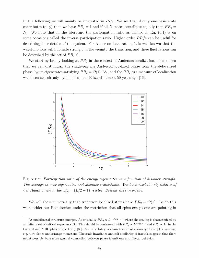
In the following we will mainly be interested in PR2. We see that if only one basis state

contributes to |ψ〉 then we have PR2 = 1 and if all N states contribute equally then PR2 =

N . We note that in the literature the participation ratio as defined in Eq. (6.1) is on

some occasions called the inverse participation ratio. Higher order PRq’s can be useful for

describing finer details of the system. For Anderson localization, it is well known that the

wavefunctions will fluctuate strongly in the vicinity the transition, and these fluctuations can

be described by the set of PRq’s†.

We start by briefly looking at PR2 in the context of Anderson localization. It is known

that we can distinguish the single-particle Anderson localized phase from the delocalized

phase, by its eigenstates satisfying PR2 = O(1) [38], and the PR2 as a measure of localization

was discussed already by Thouless and Edwards almost 50 years ago [16].

Figure 6.2: Participation ratio of the energy eigenstates as a function of disorder strength.

The average is over eigenstates and disorder realizations. We have used the eigenstates of

our Hamiltonian in the Sztot = (L/2− 1) -sector. System sizes in legend.

We will show numerically that Anderson localized states have PR2 = O(1). To do this

we consider our Hamiltonian under the restriction that all spins except one are pointing in

†A multifractal structure emerges. At criticality PRq ∝ L−Dq(q−1), where the scaling is characterized by

an infinite set of critical exponents Dq. This should be contrasted with PRq ∝ L−d(q−1) and PRq ∝ L0 in the

thermal and MBL phase respectively [38]. Multifractality is characteristic of a variety of complex systems;

e.g. turbulence and strange attractors. The scale invariance and self-similarity of fractals suggests that there

might possibly be a more general connection between phase transitions and fractal behavior.

47

the same direction, i.e. we are looking at the Sztot = (L/2−1) -sector. We let |ψ〉 be a energy

eigenstate and |α〉 the non-entangled product states in the Sztot = (L/2− 1) -sector. This

corresponds to only having one fermion in the fermionic system, and is equivalent to the

Anderson model.

We see from Fig. 6.2 that the participation ratio of the Anderson localized eigenstates

does not appear to have any systematic increase or decrease with system size, which indicates

that we have PR2 = O(1). We also see that the participation ratio decreases with increasing

W . That is, for increasing disorder the eigenstates are localized on fewer and fewer sites,

corresponding to shorter localization lengths. At very large W the the localization length is

comparable to the lattice spacing.

When discussing the scaling theory to Anderson localization we saw that in one

dimension, the system should be localized for all disorder strengths in the thermodynamic

limit, and this does indeed appear to hold for our model. We have however only considered

disorder strengths down to W = 0.5, because for very small systems the localization lengths

can be very large, even comparable to the size of the system. Thus for very small disorder

finite-size effects might make such small systems appear delocalized.

We now turn our attention back to the MBL case, and we wish to consider if we can

distinguish the MBL from the thermal phase using the PR2. We therefore look at our model

in the Sztot = 0 -sector and calculate the participation ratios of the MBL eigenstates. We start

by looking at how the probability distribution of PR2 in the MBL phase changes when we

increase L. We see from Fig. 6.3 that the participation ratio does not scale as O(1), on the

contrary it gets larger for increasing system sizes. Since PR2 is increasing with increasing L

it is problematic to use it to distinguish the thermal from the MBL phase.

The reason for the participation ratio’s increase with increasing L in the MBL phase is

that, even though we have exponentially decaying amplitudes in configuration space, we also

have a rapidly growing number of states which can lie inside the localization radius of a MBL

state. Thus since the many-body Hilbert space is growing exponentially with the number of

spins, the states will have to lie exponentially close to each other in configuration space and

thus the number of states which lie inside of the localization radius of any given MBL state

will increase with the system size.

48

Figure 6.3: Distribution of participation ratios for MBL energy eigenstates for increasingly

large systems, which all have quenched disorder from a distribution with a width W = 5.

System sizes in legend.

We will therefore instead consider the following related function

PH =PR2

N(6.2)

Where N is the size of the Hilbert space. Whereas there is an obvious physical interpretation

of PR2 ready at hand, it is not equally obvious which physical significance PH has, other

than a rescaled participation ratio. Therefore we will show that we can relate PR2 and PH

to the quantum dynamics and argue that PH can be used to pinpoint when the system enters

the MBL phase.

We consider the survival probability encoded in G(t) = 〈ψ(0)|e−iHt|ψ(0)〉, where

|〈ψ(0)|e−iHt|ψ(0)〉|2 quantifies the probability for a state to remain the same after some

time t has passed. We start by showing how the survival probability of a basis state |α〉 in

the configuration space is linked to PR2. We calculate the infinite-time average of |G(t)|2,

where the infinite-time average is taken in order to remove finite-size effects like quantum

recurrence.

49

S = limτ→∞

1

τ

∫ τ

0

dt |G(t)|2

= limτ→∞

1

τ

∫ τ

0

dt |〈α|e−iHt|α〉|2

=∑nm

|〈α|m〉|2|〈n|α〉|2 limτ→∞

1

τ

∫ τ

0

dt e−i(En−Em)t

=∑n

|〈n|α〉|4 = PR−12

(6.3)

Where we have inserted complete sets of energy eigenstates. We assumed that the system at

time t = 0 is in one of the basis states |α〉, which is an eigenstate of the disorder part of the

Hamiltonian. Starting the dynamics therefore coincides with turning on the interaction part

of the Hamiltonian, and the survival probability can thus serve as an indicator of whether or

not the system is localized.

If the system is thermal we expect that the Hilbert space will be rather uniformly explored

during the quantum dynamics, and that the survival probability is approximately inversely

proportional to the size of the Hilbert space. Therefore we expect to have S = O(1/N) for

small disorder.

Conversely if the system is MBL it must remain close to its initial state at all times because

the quantum dynamics only lets the system explore a small amount of the configuration space.

Therefore S should certainly be much larger in the MBL phase than in the thermal phase.

We define Serg = 1/N as the survival probability for an ideal ergodic system. We then have

PH = Serg/S, and we can use PH to measure whether the system is localized or not. When

we increase the system size, PH must approach zero in the MBL phase, whereas it remains

finite in the thermal phase.

We can also make a more detailed prediction for PH in the thermal phase, since we expect

that Berry’s conjecture holds and that GOE should describe the statistical behavior of the

eigenvectors’ weights |〈n|α〉|. Then |〈n|α〉| are Gaussian random numbers for which Isserlis’

therem holds, as in Eq. (3.21), and PH should approach 1/3 in the ergodic phase for N →∞.

We can use 〈PH〉 in Fig. 6.4 to distinguish between the MBL and the thermal phase.

We see that 〈PH〉 is clearly tending towards zero in the thermodynamic limit for disorder

strengths greater than W ≈ 3. For W . 2.5, it appears that 〈PH〉 approaches finite values

when we increase the system size. That is, for small disorder the survival probability does

indeed scale as 1/N and the system is thermal.

50

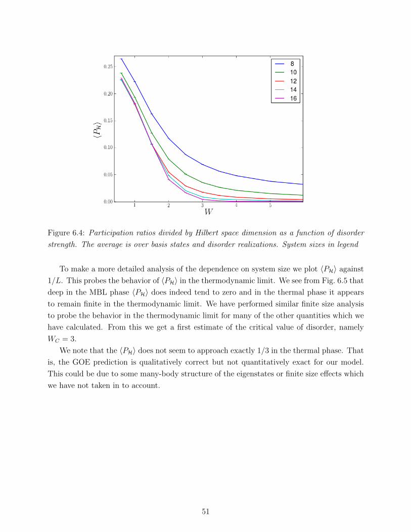
Figure 6.4: Participation ratios divided by Hilbert space dimension as a function of disorder

strength. The average is over basis states and disorder realizations. System sizes in legend

To make a more detailed analysis of the dependence on system size we plot 〈PH〉 against

1/L. This probes the behavior of 〈PH〉 in the thermodynamic limit. We see from Fig. 6.5 that

deep in the MBL phase 〈PH〉 does indeed tend to zero and in the thermal phase it appears

to remain finite in the thermodynamic limit. We have performed similar finite size analysis

to probe the behavior in the thermodynamic limit for many of the other quantities which we

have calculated. From this we get a first estimate of the critical value of disorder, namely

WC = 3.

We note that the 〈PH〉 does not seem to approach exactly 1/3 in the thermal phase. That

is, the GOE prediction is qualitatively correct but not quantitatively exact for our model.

This could be due to some many-body structure of the eigenstates or finite size effects which

we have not taken in to account.

51

Figure 6.5: Finite size scaling of 〈PH〉. Disorder strengths in legend

6.1.2 Information Entropy

The MBL eigenstates are localized in a small portion of the basis states in configuration space

whereas the thermal eigenstates generally are spread out over most of the configuration space

basis.

In this sense, when expressed in the non-entangled product state basis, the energy

eigenstates are more complex in the thermal phase than in the MBL phase. We will in the

following quantify this by using the information entropy as a measure of complexity, and we

consider the Shannon entropy defined as

In = −∑α

|〈n|α〉|2 log(|〈n|α〉|2

)(6.4)

The information entropy says something about the interrelation between the energy

eigenstates basis and the product space basis and it quantifies the complexity of their

relationship. We thus use In to probe how localized the energy eigenstates are in

configuration space. If the eigenstates are completely localized in configuration space we get

Cαn = δnα and thus zero complexity, and if the eigenstates are uniformly spread out over

the non-entangled product states we have maximal complexity log(N). We thus expect the

complexity to be almost maximal deep in the thermal phase and diminish as we increase the

disorder.

We expect that the MBL eigenstates are not completely localized but rather spread out

over a small portion of the configuration space, and that an increasing number of basis states

52

contributes to the eigenstates for increasing system sizes. Thus the number of non-zero Cαn ’s

should increase with N . We will naively assume that the MBL eigenstates are uniformly

spread out over N ν basis states, where ν ∈ [0, 1] ⊂ R. This is indeed an oversimplification

since we have expect to have exponentially localized states, and therefore the non-zero Cαn ’s

are not going to be equal. However, it could still serve as a crude measure of how how many

of the product states contribute to the MBL states. Under this assumption we get

I(loc)n = −

Nν∑α=1

| 1√N ν|2 log

(| 1√Nν|2)

=Nν∑α=1

N−ν log(N ν)

= ν log(N)

(6.5)

We thus expect the complexity of the system to increase with increasing system size, and that

the complexity differs from the maximal complexity by a factor ν, which is some admittedly

naive measure of how many of the product states contribute to an MBL state. Since the MBL

eigenstates are localized only on a small number of states, there should not be any significant

finite size effects to this approximation, and it should be equally good for all system sizes.

We expect ν to be approximately independent of system system size, since the number of

states inside the localization radius of a MBL state should increase at the same rate as the

size of the Hilbert space. This is because the localization length is only weakly dependent

on L whereas the Hilbert space grows exponentially in L.

In the thermal phase we expect that GOE will describe the statistics of the system

asymptotically for increasing N ’s. As discussed in Chap. 3 the eigenvectors of the GOE in

N dimensions projected onto a fixed basis have a Gaussian distribution of its components

P (Cαn ) ∝ e−

N2|Cαn |2 (6.6)

Where Cαn = 〈n|α〉. For such states the information entropy has been shown to be I

(GOE)n =

log(0.482N) + O(1/N) in Ref. [52], which we see rapidly approaches maximal entropy. For

realistic systems this presumably serves as an upper bound on the information entropy. Both

since the GOE only accurately describes the eigenvectors statistics for large N and since

the GOE prediction entropy only asymptotically approaches log(N) with increasing N , the

information entropy in the thermal phase should initially be much smaller than log(N) but

quickly approaching log(N) as we increase N .

We calculate the information entropy divided by maximal entropy numerically in Fig. 6.6.

We see that when we take the thermodynamic limit, IN/ log(N) appears to be approaching

unity for small W and for larger W we see that IN/ log(N) is only weakly dependent on N and

decreasing with increasing disorder. This means that when we approach the thermodynamic

limit, we tend toward maximally complex eigenstates in the thermal phase and in the MBL

53

phase the complexity is O(log(N)). We note that although In ∼ O(log(N)) holds in the

MBL phase we see that, apart from for L = 8, IN/ log(N) is slightly larger for larger N

and this is consistent with a weak dependence of the localization length on the system size.

We can then approximate the critical value of disorder by the value for which In/ log(N)

gets roughly independent on the system size. We thus see that WC = 3.4 appears to be the

critical value of disorder strength.

Figure 6.6: Information entropy divided by maximal entropy as a function of disorder strength.

The average over eigenstates and disorder realizations. System sizes in legend

6.2 Absence of Level Repulsion

We will now consider the spectral statistics of our many-body Hamiltonian. The BGS

conjecture states that the statistics of thermal systems should be like that of the appropriate

RMT ensemble. Since the MBL phase in some respect is similar to an integrable system,

we expect the statistics in the MBL phase to have Poisson statistics, which according to the

Berry-Tabor conjecture is the case for integrable systems. We know that in GOE statistics,

the levels repel each other, whereas Poisson statistics has no such level repulsion. This is

believed to be a distinguishing characteristic of the MBL phase.

If we assume our model to support LIOM’s we can easily argue that the levels do not

repel each other. This is because adjacent energy levels in the spectrum typically differ by

an extensive amount of eigenvalues of the τj’s. Therefore the levels cannot hybridize and do

not repel on the scale of the mean level spacing.

54

We calculate the energy difference between adjacent states in the spectrum and show

histograms of the level spacings in the thermal and MBL phase in Fig. 6.8. We see that they

fit very nicely with the Wigner Surmise and Poisson distribution respectively, and we clearly

see the level repulsion in the weak disorder regime, and the absence thereof in the strong

disorder regime.

(a) Thermal phase (b) MBL phase

Figure 6.7: The distribution of energy level spacings in the thermal and MBL phase. We

found the level spacing ∆ for different eigenstates and different realizations of disorder for

systems of size L = 14.

We would like to study the crossover between GOE and Poisson statistics in our model

and pinpoint at which disorder strength the MBL transition is.

The choice of quantity to use for such a finite-size scaling analysis is to some degree

arbitrary, and there are many different quantities which we could have used. We need a

dimensionless measure of the statistics of spectral properties, which in the thermodynamic

limit takes different finite values in the ergodic and MBL phase. Generally when we want

to compare energy level spacings we first need to perform an unfolding procedure, to ensure

that the mean level spacing is set to unity. For that reason we will follow Refs. [4, 53] and

consider the following function which requires no unfolding

r(n) =min∆n,∆n−1max∆n,∆n−1

(6.7)

Where ∆n = |En −En−1| and we assume that the energy levels En are listed in ascending

order. This function requires no unfolding since it only compares ratios of gaps between

energy levels. We will calculate expectations values of r(n) for the energy levels of our

Hamiltonian and compare this to GOE and Poisson statistics. The expectation value of

r(n) is calculated in Appendix B to be 〈r(n)〉Poisson ∼= 0.39 and 〈r(n)〉GOE ∼= 0.53 for spectra

following Poisson and GOE statistics respectively.

55

Figure 6.8: The ratio of adjacent energy gaps as a function of disorder strength. The average

is over disorder realization and eigenstates. System sizes in legend.

We see from Fig. 6.8 that 〈r(n)〉 is rapidly approaching the GOE and the Poisson

expectation values with increasing L, for small and large W respectively.

We note that our model is integrable at zero disorder, thus 〈r(n)〉 might not show GOE

statistics in this limit. We presumably see signs of this for L = 8 and small W . It was argued

by Deutsch [11] that integrable many-body systems become thermal upon an arbitrary small

perturbation of the Hamiltonian in the form of a random matrix. However his argument

relied upon having systems with many degrees of freedom. This could explain why 〈r(n)〉appear to not approach 〈r(n)〉GOE for small values of L and W .

We estimate the location of the transition by considering the crossing of the curves for

different values of L. These crossings are drifting towards the localized phase, however the

drift is only very slight and is decreasing with increasing L. In Ref. [53] they were not able

to say something conclusive about whether this drift will diminish or continue indefinitely,

and they argued that this drift could stem from that behavior of the system in the critical

region in some sense is more like the MBL phase. Although any proper finite-size scaling is

difficult, we argue as in Ref. [4] that the crossings appear to converge to a finite WC . Thus

we conclude that the plot indicates that there will be a phase transition at a finite disorder

strength, which we from Fig. 6.8 thus estimate to be at WC = 3.1.

56

6.3 Area Law Entanglement

We will in this section consider the entanglement between two subsystems. Thermal systems

are known to have entanglement which follows a volume law O(Ld) whereas MBL systems

have area-law entanglement O(Ld−1). Area-law entanglement is known to occur in certain

quantum ground states of gapped Hamiltonians, but we will see that also highly excited MBL

states have entanglement which scales as O(Ld−1).

We can see that MBL systems have area-law entanglement by assuming that our model

supports LIOM’s. The eigenstates of our Hamiltonian is then product states of the τj’s and

when we split the system in two and consider the entanglement between the subsystems, we

only get contributions to the entanglement from the integrals of motion which are localized

within a distance ξ away from the cut. Thus the entanglement scales as the area separating

the subsystems and not the volume of the subsystems.

We will start by discussing and defining entanglement entropy in more detail and then

we consider the entanglement in a thermal system more thoroughly, before we discuss our

numeric results.

6.3.1 Bipartite Entanglement Entropy

A quantum system can have correlations which cannot be described by classical mechanics.

This is called entanglement and is one of the fundamental features of quantum mechanics. In

the following we describe bipartite entanglement mathematically. Bipartite means we have

entanglement between exactly two subsystems†. We consider a system with Hilbert space H,

which we divide into the subsystems S and B such that H = HS ⊗HB. Then a general state

in H can be expressed as

|ψ〉 =

NS∑n=1

NB∑m=1

Cnm|n〉S ⊗ |m〉B (6.8)

We have the density operator defined as

ρ =∑n

pn|ψn〉〈ψn| (6.9)

where |ψn〉 is some ensemble of states which are on the form of Eq. (6.8), and pn is the

“classical” probability for having the system in state |ψn〉. If we assume |ψn〉 to be normalized

to unity the density operator need to satisfy the following conditions

trρ = 1

ρ† = ρ

〈ψ|ρ|ψ〉 ≥ 0 ∀|ψ〉

(6.10)

†There is no unambiguously way to define multipartite entanglement

57

If one of the pn’s is one and all the others are zero we call it a pure state. From now

on we restrict our discussion to pure states, since we will later measure entanglement of

systems which we know are in their energy eigenstate, and as such we have maximal “classical

information” about the system. A pure state is said to be quantum mechanically entangled

if it cannot be expressed as a product state, i.e. if

|ψ〉 6= |φ〉S ⊗ |ξ〉B (6.11)

Which is the case if it is not possible to express the weights in Eq. (6.8) as CSnCBm. Since we

have maximal classical information about the full system, these correlations between the two

subsystems are purely quantum in nature.

The reduced density matrix is obtained by tracing out the degrees of freedom of one of the

systems, e.g. ρS = trBρ, and this density matrix also satisfies the constraints of Eq. (6.10).

The standard way of studying the entanglement is to look at the spectrum σ(ρS) = λn.The normalization and positivity restrictions leads us to think of λn as a probability

distribution. A distribution dominated by one value of λn close to one and the rest roughly

zero is less entangled than a more uniform distribution. In analogy with statistical physics we

assign an entropy to this probability distribution, namely the von Neumann entropy defined

as

SS = − tr(ρS logρS

)= −

∑i

λilogλi(6.12)

Here we see that a minimally entangled state has SS = 0, while a maximally entangled state

has SS = log(N). We interpret the von Neumann entropy of the ρS as a measure of how

many degrees of freedom in S are entangled with degrees of freedom in B. We assumed our

system to be in a pure state, which means that the von Neumann entropy SF of the full

system is zero. It holds for quantum systems that

SF ≤ SS + SB ∧ SF ≥ |SS − SB| (6.13)

Where this should be contrasted with the classical constraints on entropy SF ≥ maxSS , SB.In the classical regime the full system cannot be less ordered than its parts, whereas for

quantum system the full system’s entropy can indeed be less than that of its parts. We thus

have that in the case where the full system F is in a pure state the von Neumann entropy of

the two subsystems are equal and we call this the entanglement entropy SE.

Entanglement in a Thermal System

We will assume a thermal system and consider what the entanglement entropy between

the B and S of a full system in an energy eigenstate should be. We assume that thermal

58

systems satisfy Berry’s conjecture, and that we therefore can write a general eigenstate as

|n〉 =∑N

k=1Rk|α〉 where Rk is some Gaussian random number. We comsider the state in

terms of its two subsystems S and B.

|n〉 =

NS∑=1

NB∑β=1

Rα|α〉S ⊗ |β〉B (6.14)

Where we have changed indices on the random variable, which we can do since N = NBNS .

This gives us the following form of the density matrix for the full system

ρ(n) =

NS∑α,β=1

NB∑γ,δ=1

RαγR∗βδ|α〉S〈γ|S ⊗ |β〉B〈δ|B (6.15)

We wish to consider the reduced density operator, so we trace out the degrees of freedom in

B which we assume to be the larger of the two subsystems and we get

ρ(n)S = trB ρ =

NS∑α,γ=1

NB∑β=1

RαβR∗γβ|α〉S〈γ|S

=S∑

α,γ=1

Xαγ|α〉S〈γ|S

(6.16)

Where we have X = RR† as a NS × NS-matrix and R is a NS × NB-matrix. The matrix

elements of R are by assumption i.i.d. Gaussian random numbers and for the sake of

generality we assume X to be unitary. Such matrices are called Wishart matrices and they

have the following probability distribution

P (X) =1

2NBNS

2 Γp(NB2

)|Σ|NS2

|X|NB−NS−1

2 e−12

trΣ−1X (6.17)

Where Σ is the covariance matrix and Γp(x) the multivariate gamma function. These types

of matrices have been thoroughly studied for many years. If we assume the normalization

constraint∑

n λn = 1 on the spectrum λn, the joint probability distribution of the

eigenvalues of X is given by

P (λn) ∝ δ( NS∑n=1

λn − 1) NS∏n=1

λNS−NBn

∏k<l

(λk − λl)2 (6.18)

Wishart matrices have also been studied in the context of entanglement entropy in random

pure states and the average entropy of a subsystem S where 1 << NS ≤ NB has been

considered in [42, 43]. They assumed a that the spectrum of the reduced density matrix was

described by Eq. (6.18), and then calculated the average entanglement entropy to be

〈SE〉 = ln(NS)− NS2NB

(6.19)

59

Where we see that a random pure state has bipartite entanglement entropy which is

dependent on the volume of the subsystem and that the states are almost maximally

entangled.

We will calculate the entropy of entanglement between two halves of our spin chain

numerically, and we will use the full Hamiltonian with all of its Sz -sectors. Since NB =

NS = 2L/2 we expect that the average entropy to be 〈SE〉 = L ln(2)/2− 1/2 in the thermal

phase.

Figure 6.9: The entropy of entanglement between two subsystems of equal size for a full

system in its energy eigenstate as a function of disorder. The average is over eigenstates and

disorder realizations. We have considered the full Hamiltonian, not just the Sz = 0 -sector.

The dotted line is the thermal entanglement entropy. Disorder strength in legend.

We see from Fig. 6.9 that deep in the thermal phase the average entropy scales roughly as

Eq. (6.19) and in the localized phase the entanglement entropy in our one-dimensional system

does not change significantly when we increase the system size. That is, the entanglement

scales as a volume-law in the thermal phase and an area-law in the MBL phase.

6.4 Failure to Thermalize

An essential characteristic of MBL systems is that they are unable to thermalize under their

own dynamics. We can see this from the assumption that MBL systems supports LIOM’s. We

then get that the quasi-locality of the τj’s imply that information about the initial conditions

is stored in the system at all times. This means that no information can be exchanged on

the scale of the system size and thus the system fail to reach thermal equilibrium.

60

6.4.1 Violation of the ETH

We would now like to test the ETH, which claims that single energy eigenstates should

reproduce the microcanonical ensemble average at given energy. For this to happen we

need that the difference of the expectation values of a local operator in two adjacent energy

eigenstates should be vanishingly small when approaching the thermodynamic limit. We let

Szi be our local operator and we consider the magnetization in energy eigenstates mi,n, and

if the ETH is satisfied it must hold that

mi,n+1 −mi,n → 0 (6.20)

That is, the difference in eigenstate expectation values of Szi between two adjacent eigenstates

should decrease exponentially when we increase L.

Assuming that in the MBL phase there exist LIOM’s which are weak deformation of the

local degrees of freedom, namely the spin-operators, we typically get mi,n ≈ ±1/2. Since the

adjacent energy eigenstates generally differ in an extensive amount of eigenvalues of the τj’s,

mi,n+1 −mi,n is thus equally likely to evaluate to approximately zero and to approximately

one. We therefore expect that in the MBL phase 〈mi,n+1 −mi,n〉 ≈ 1/2.

Figure 6.10: The difference of expectation values of Szi in adjacent energy eigenstates as a

function of disorder. The average is over sites, disorder realizations and eigenstates. System

sizes in legend.

We see clearly from Fig. 6.10 that for small disorder the difference in magnetization

becomes exponentially small when we increase the system size. That 〈mi,n+1 −mi,n〉 tends

exponentially fast to zero with increasing L pertains up to disorder strength W ≈ 4, but

61

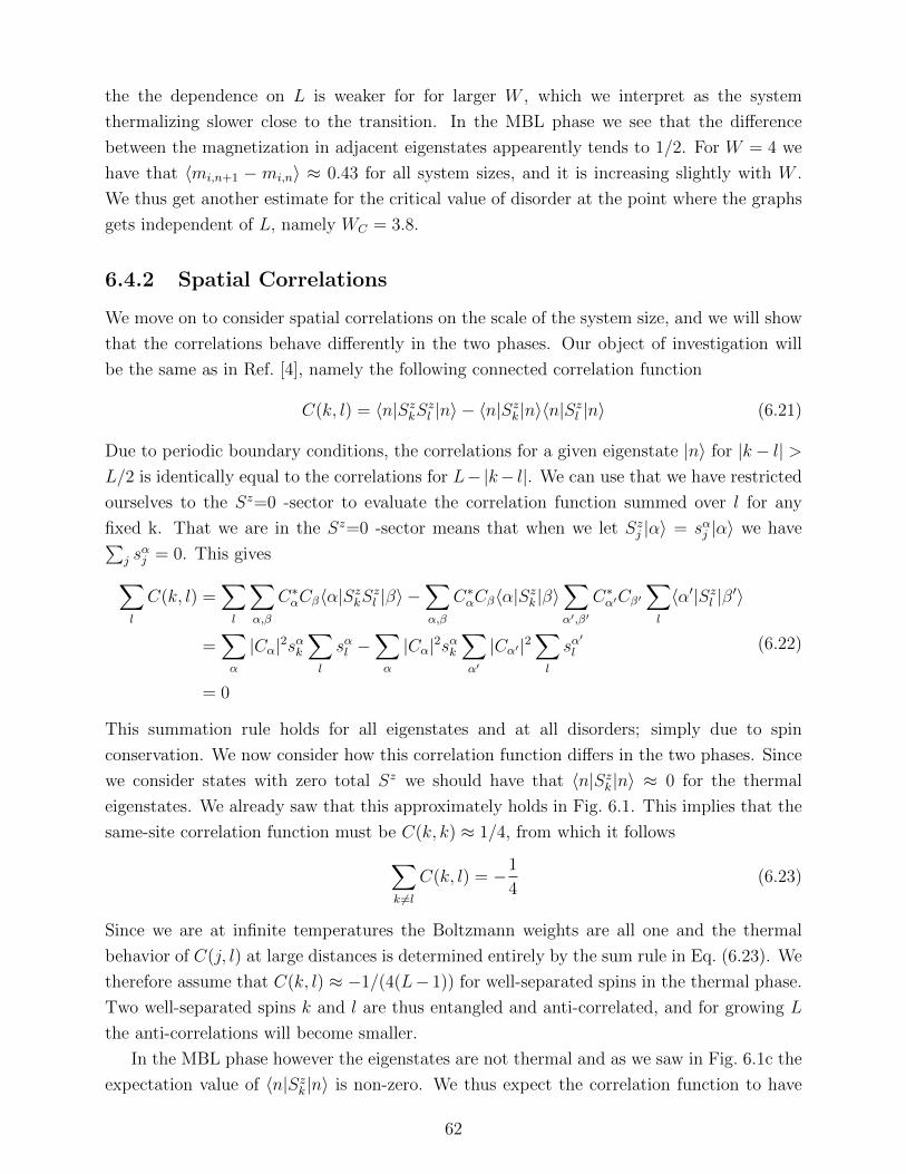
the the dependence on L is weaker for for larger W , which we interpret as the system

thermalizing slower close to the transition. In the MBL phase we see that the difference

between the magnetization in adjacent eigenstates appearently tends to 1/2. For W = 4 we

have that 〈mi,n+1 − mi,n〉 ≈ 0.43 for all system sizes, and it is increasing slightly with W .

We thus get another estimate for the critical value of disorder at the point where the graphs

gets independent of L, namely WC = 3.8.

6.4.2 Spatial Correlations

We move on to consider spatial correlations on the scale of the system size, and we will show

that the correlations behave differently in the two phases. Our object of investigation will

be the same as in Ref. [4], namely the following connected correlation function

C(k, l) = 〈n|SzkSzl |n〉 − 〈n|Szk |n〉〈n|Szl |n〉 (6.21)

Due to periodic boundary conditions, the correlations for a given eigenstate |n〉 for |k− l| >L/2 is identically equal to the correlations for L−|k− l|. We can use that we have restricted

ourselves to the Sz=0 -sector to evaluate the correlation function summed over l for any

fixed k. That we are in the Sz=0 -sector means that when we let Szj |α〉 = sαj |α〉 we have∑j s

αj = 0. This gives∑

l

C(k, l) =∑l

∑α,β

C∗αCβ〈α|SzkSzl |β〉 −∑α,β

C∗αCβ〈α|Szk |β〉∑α′,β′

C∗α′Cβ′∑l

〈α′|Szl |β′〉

=∑α

|Cα|2sαk∑l

sαl −∑α

|Cα|2sαk∑α′

|Cα′|2∑l

sα′

l

= 0

(6.22)

This summation rule holds for all eigenstates and at all disorders; simply due to spin

conservation. We now consider how this correlation function differs in the two phases. Since

we consider states with zero total Sz we should have that 〈n|Szk |n〉 ≈ 0 for the thermal

eigenstates. We already saw that this approximately holds in Fig. 6.1. This implies that the

same-site correlation function must be C(k, k) ≈ 1/4, from which it follows∑k 6=l

C(k, l) = −1

4(6.23)

Since we are at infinite temperatures the Boltzmann weights are all one and the thermal

behavior of C(j, l) at large distances is determined entirely by the sum rule in Eq. (6.23). We

therefore assume that C(k, l) ≈ −1/(4(L− 1)) for well-separated spins in the thermal phase.

Two well-separated spins k and l are thus entangled and anti-correlated, and for growing L

the anti-correlations will become smaller.

In the MBL phase however the eigenstates are not thermal and as we saw in Fig. 6.1c the

expectation value of 〈n|Szk |n〉 is non-zero. We thus expect the correlation function to have

62

an amplitude which falls off exponentially with distance due to the exponential localization

of spins in configuration space. That is, we expect

C(k, l) ∼ e−|k−l|ξ (6.24)

Where ξ is the localization length. If we assume that our model supports LIOM’s this follows

naturally, since we can think of the LIOM’s as dressed spins. Therefore the exponential

localizations of the τj’s imply that the spins far away from each other will not influence each

other significantly.

Whereas we expect mostly negative correlations in the thermal phase, we have no reason

to expect any particular sign of the correlations in the MBL phase.

(a) W=1 (b) W=6

Figure 6.11: The logarithm of the correlation function C(i, i + d) as a function of d. The

average is over eigenstates, disorder realizations and i, and the disorder distribution have a

width of W . System sizes in legend

We see from Fig. 6.11 that the correlations in the MBL phase do indeed fall off

exponentially with increasing d, except for d close to L/2, due to periodic boundary

conditions. In the thermal phase the correlations are roughly constant for large d and

smaller for larger systems, as we expected. We have used the absolute value of the

correlations in Fig. 6.11 but we wish to also consider if the system tends to have mostly

correlations or anti-correlations. We therefore check that in the MBL phase the correlations

do indeed have random signs, whereas the correlations are mostly negative in the thermal

phase. We quantify this by considering the function

NC =N− −N+

N− +N+

(6.25)

Where N+ and N− is the number of eigenstates for which the correlation function C(i, i+L/2)

is positive and negative respectively.

63

Figure 6.12: The excess number of states with anti-correlations at distance L/2. We first

estimated NC by counting eigenstates and sites for each disorder realization, and the error bars

were then found by considering the differences in NC between different disorder realization.

System sizes in legend.

We calculated the long-distance correlation function and found NC for different system

sizes and disorder strengths, and the results are shown in Fig. 6.12. We see that deep in the

thermal phase almost all of the eigenstates show negative correlations and that NC tends to

one for small disorder. In the MBL phase the signs of the correlations are seemingly random

and NC tends towards zero. We use the crossing of the curves as an estimate for the critical

value of disorder and we notice a very slightly drifting towards larger W for increasing L. The

drift does however appear to diminish and we conclude that the transition between mostly

anti-correlations to randomly signed correlations suggest that WC = 3.

6.5 Absence of DC Transport

We will in this section show that there is no transport of conserved quantities in the MBL

phase. For an Anderson localized system this is rather obvious since its wavefunctions are

localized in a finite region of space. However, MBL system have eigenfunctions which are

extended in real space so it is not equally obvious that conserved quantities cannot be carried

over large distances.

It was shown by Basko et al. [2] that the MBL states they considered have zero

conductivity. It does not necessarily need to be any absence of transport for MBL to

occur, since MBL has been shown to exist also in Floquet systems, which generally have

64

no conserved quantities and thus no transport [26, 41]. In the following we will argue that

LIOM’s suppress transport and we will show numerically that there is no transport of spin

in the random-field Heisenberg model.

6.5.1 Absence of DC Transport in a Model with LIOM’s

We argue that a complete set of constants of motions suppress transport, following the

arguments of Ros, Mueller and Scardicchio [50]. We first show that the DC conductivity

is zero when our model has strictly local integrals of motion. We then also argue that the

argument should hold also for quasi-local integrals of motion, but this can only be seen

rigorously from the convergence of the perturbative construction of the LIOM’s in Ref. [50].

In Appendix C we use the Kubo formula for the conductivity tensor to show that the DC

conductivity is governed by

<σ(ω → 0) =πβ

ZΩ

∑r′r

∑nm

〈n|Jr+r′|m〉〈m|Jr|n〉e−βEnδη(Em − En) (6.26)

Where Ω is the volume of the system and Jr the local current density. We first assume that

the integrals of motion are strictly local, i.e. their support is restricted to a small region

of diameter ξ. The energy eigenstates can be completely determined by the eigenvalues of

the LIOM’s, due to the completeness of the set of integrals of motion. For two different

eigenstates, there will therefore always exist integrals of motion which have different

eigenvalues for the two states. We assume τ to be such an integral of motion for the two

states |m〉 and |n〉. We then have

τ |m〉 = τm|m〉 ∧ τ |n〉 = τn|n〉 (6.27)

Where τm 6= τn, where τm and τn are the eigenvalues of τ . This allows us to write the all of

the matrix elements of the current operators as

〈m|Jr|n〉 =〈m|[Jr, τ ]|n〉τn − τm

〈n|Jr′+r|m〉 =〈n|[Jr′+r, τ ]|m〉

τm − τn

(6.28)

Where the τ is different for the different matrix elements. Since we assumed strictly local

integrals of motion and the current operators are local, one of these terms has to vanish when

r′ is larger than ξ, since one of the commutators then evaluates to zero. That is, the sum

over r in Eq. (6.26) is restricted to r . ξ.

Furthermore the locality of the τj’s and Jr, implies that Jr|n〉 is different from |n〉 only

for a finite number of τj’s. This is because we have LIOM’s whose eigenvalues unequivocally

determine the eigenstates of the Hamiltonian, and we therefore have

Jr|n〉 = Jr|τn1 , τn2 , . . . τnN 〉∝ |τn1 , . . . Jrτni , Jrτni+1

, Jrτni+2, . . . τnN 〉

(6.29)

65

That is, the current operator only affect the τj’s whose support overlap with that of Jr’s.

For a given r and |n〉 the matrix element 〈m|Jr|n〉 can thus be non-zero only for the m’s

which have the same eigenvalue as |n〉 for all the LIOM’s whose support do not overlap with

Jr’s support. This means that for every m the sum over n is restricted to a finite set. The

eigenstates for which 〈m|Jr|n〉 is non-zero do not have to be close in energy, because adjacent

energy levels in the spectrum typically differ in an extensive number of eigenvalues of the

LIOM’s. Therefore the contribution to the delta function goes to zero when we take the

thermodynamic limit and send η → 0.

Thus we have shown that <σ(ω → 0) = 0 in a system with strictly local integrals of

motion. However the LIOM’s in MBL systems are be quasi-local. Quasi-locality implies

that the matrix elements 〈m|Jr|n〉 for eigenstates |m〉 and |n〉 who are different only in

integrals of motion which are centered up to a distance xξ away from r, do no longer

need to be zero. They will be exponentially small in x, but there are exponentially

many states m and n that satisfies this criteria. So some energy differences Em − En

in Eq. (6.28) might become exponentially small. The energy denominators are however

dominated by the exponential decay of the matrix elements with probability one, and

this is the key statement that guarantees the stability of the MBL. To see explicitly why

this is the case we refer to Ref. [50], and their perturbative construction if the LIOM’s.

The convergence of the construction procedure ensures that the exponential smallness

of the energy denominators is dominated by the decay of the matrix elements and that

the contribution to the δ-function is zero also for a system with quasi-local integrals of motion.

6.5.2 Absence of Spin Transport in our Model

There are two conserved quantities in our model, namely total Sz and energy. We have

showed that the system fails to thermalize in the MBL phase, and this implies that there

are no transport of energy. We will now show numerically that there is also no transport of

spin in our random-field Heisenberg model. We will largely follow Ref. [4] and consider the

longest wavelength Fourier mode of the spin density

M =L∑j=1

Szj e2πiLj (6.30)

We wish to study transport over long length scales and therefore look at the relaxation of

an initial inhomogeneous spin density given by M . We assume to have prepared our system

with a tiny modulation of order ε of the spin density in this mode and that the initial density

operator for the system is

ρ(0) =eεM

†

Z≈ 1 + εM †

Z(6.31)

66

Where we have used that we have β = 0 and that ε is very small. The initial spin polarization

of this mode is then

〈M〉0 = trρ(0)M =ε

Z

∑n

〈n|M †M |n〉 (6.32)

We now wish to consider how this initial spin polarization evolves in time. We are in the

Schrodinger-picture so the density matrix is evolved in time by the unitary exp(−iHt) and

get the following expectation value for M at an arbitrary time t

〈M〉t = trρ(t)M= tre−iHtρ(0)eiHtM

=ε

Z

∑nm

|〈m|M |n〉|2ei(En−Em)t

(6.33)

We take the infinite-time average of 〈M〉t and get that it is diagonal in the energy eigenstates

basis. We have

〈M〉∞ = limτ→∞

∫ τ

0

dt trρ(t)M

=ε

Z

∑n

〈n|M †|n〉〈n|M |n〉(6.34)

If there is transport over long distances the initial spin polarization should decay away with

time, and therefore the initial spin polarization should not equal the infinite-time averaged

polarization. We thus expect that in the MBL phase 〈M〉0 ≈ 〈M〉∞ should hold, whereas

in the thermal phase we expect that 〈M〉0/〈M〉∞ → 0. To test this we define the following

function as a measure of how much of the contribution to 〈M〉 from an energy eigenstate |n〉is dynamic and therefore decays away

fn = 1− 〈n|M†|n〉〈n|M |n〉

〈n|M †M |n〉(6.35)

This function should approach zero in the MBL phase since the spin polarization is not

transported away, and conversely in the thermal phase the spin polarization should decay

and fn should approach one.

We do indeed see from Fig. 6.13 that fn appears to approach zero as we increase L in the

MBL phase, i.e. that there is no long distance spin transport. In the thermal phase fn quickly

approaches one for large L, which means that the polarization decays under the dynamics.

We use the points of crossing of the lines for different system sizes as an estimate for WC .

In contrast to Ref. [4] we find a somewhat slighter drift of the crossings, and it appears that

the critical point is at WC = 3.1.

67

Figure 6.13: Transport of spin on the scale of the system size as a function if disorder

strength. We have measured spin transport through the function fn as defined in Eq. (6.35).

The average is over eigenstates and realizations of disorder. System sizes in legend.

68

Chapter 7

The Phase Transition & Universality

We have in Chap. 6 shown that our model has two distinct phases with very different

properties, and we have argued through finite size scaling that the phase transition is at

finite values of W . We will in the following consider the MBL transition itself in more detail.

Unlike most quantum phase transitions the MBL transition occurs for non-zero, and even

infinite, temperatures. Or more precisely at energy densities, which would correspond to

finite temperatures if the system was thermal. We will assume that the MBL transition is a

continuous phase transition with a vanishing characteristic energy scale δC , and a diverging

characteristic length scale lC .

We start by discussing which role disorder plays in determining the critical behavior and

how we can use the renormalization group on systems with disorder. We will then use some

results from the strong disorder renormalization group and argue that the MBL transition

is governed by a fixed point with infinite randomness. We shall also consider the long-time

dynamics near the transition and argue that there is a broad critical region near the phase

transition and show that the dynamics can be sub-diffusive in the thermal phase.

7.1 Critical Phenomena & the Renormalization Group

We will in the following briefly discuss some ideas of the renormalization group in the

context of phase transitions in general and the strong disorder renormalization group in

particular. Renormalization was first consider in particle physics and was used in quantum

electrodynamics by Gell-Mann and Low [60]. In the context of critical phenomena such ideas

were considered in 1966 by Kadanoff [61], when he considered “block-spin renormalization”.

He blocked the components of his model together to define the components at a large scale

in terms of the components at shorter distances, and by this coarse graining he was able

to extract essential features of the macroscopic system near criticality. The renormalization

group was subsequently properly developed into a powerful calculational tool by Wilson [62]

69

in 1971, as he formalized and generalized the ideas of Kadanoff.

7.1.1 The Renormalization Group

A hallmark of critical phenomena is that fluctuations appear simultaneously at all length

scales and this causes non-analytic behavior of physical quantities. These singularities make

perturbative approaches inappropriate. The renormalization group is a mathematical tool

which we can use to systematically look at how a physical system appears when viewed at

different length scales. The basic concept is to follow the change of physical quantities as we

increase the length scale by coarse graining and rescaling, and these operations constitute

the essence of the renormalization group transformation. We assume a Hamiltonian H and

denote the renormalization group transformation

H ′ = Rb(H) (7.1)

Where Rb generally is a complicated non-linear transformation, and the system described by

H ′ is now identical to that described by H except that the spacing between the degrees of

freedom has increased by b. Rb reduces the total number of degrees of freedom by a factor

of b−d and length scales by b−1.

The renormalization transformation is a map in Hamiltonian space that mathematically

defines a semi-group. It is a semi-group because, although it has an identity operation

H = R1(H) and is associative Rb1b2(H) = Rb1Rb2(H), it has no inverse mapping. The

reason for the nonexistence of R−1b is that when we perform the coarse graining we trace out

many of the degrees of freedom and information is irretrievably lost. Exactly how Rb looks

is dependent upon the system in question.

The features of the system near criticality should only depend on a small number of

variables such as dimensionality, symmetry and range of interactions. Thus when the

renormalization group transformation removes the short-range details of the system, we

should see that many properties are independent of its microscopical details. This is

called universality and systems belonging to the same universality class have equal critical

exponents.

It is generally the case that after applying the renormalization transformation many times

the system asymptotically approaches a fixed point

H∗ = limn→∞

Rnb (H) (7.2)

Where the Hamiltonian at a fixed point is defined through H∗ = Rb(H∗). Lengths scales

are reduced by a factor of 1/b after renormalization, and in particular the correlation

length renormalizes as ξ = b−1ξ. Since the system is invariant under the renormalization

transformation at fixed points the correlation length must be either infinite or zero. We

70

call fixed points with infinite correlation length critical fixed points, whereas “trivial” fixed

points have correlation length equal to zero.

To make calculations with the renormalization group we write the Hamiltonian in terms

of the parameters ~u and the operators ~O as H = ~u · ~O, and consider how the parameters

change under renormalization. We have the renormalization group equation ~u′ = R~u, or

on continuous form d~u/d log(b) = β(~u). The beta function β(~u) encodes the parameters’

dependence on the scale b and its zeros define the fixed points. The renormalization group

equation determines the flow towards and away from the fixed points in parameter space††.

Critical fixed points repel the renormalization flow and describe the singular critical behavior,

whereas the “trivial” fixed points attract the renormalization flow and describe the phases

of the system.

7.1.2 Strong Disorder Renormalization Group

We will now discuss how we can use the renormalization group on strongly disordered

systems, a subject which was originally developed by Dasgupta and Ma [63], and eventually

given a firm theoretical footing by Fisher [65, 66]. Systems with disorder may be classified

according to which effect the disorder has at large length scales and we divide into three

cases. First we have systems controlled by pure fixed points, for which the disorder tends

to average out on large length scales and does not play any role in determining critical

behavior. Second, we have systems for which the effective disorder converges to a finite

level. Such systems are said to be controlled by a finite disorder fixed point. Third we have

systems governed by infinite disorder fixed points, and such systems have effective disorder

which grows without bound when we coarse grain them and the disorder dominate with

respect to thermal or quantum fluctuations near criticality. It is the latter case which will

interest us in the following.

Whereas renormalization in systems without disorder involves a finite number of

parameters, the strong disorder renormalization group involves probability distributions

ρ0(h)dh, describing the disorder. Therefore the analysis of the fixed points and how the

systems evolve under renormalization transformations generally becomes much harder.

The various strong disorder renormalization groups have different implementations of the

renormalization transformation but there are some properties which are general. First the

renormalization should concern the degree of freedom with the highest energy, and this high

energy grain constitutes the scale of renormalization. Second the renormalization should be

local in real space and only be concerned with the immediate neighbors of the largest valued

††The “Gang of Four” scaling theory was essentially an application of the renormalization group, where

they assumed a one-parameter scaling [17].

71

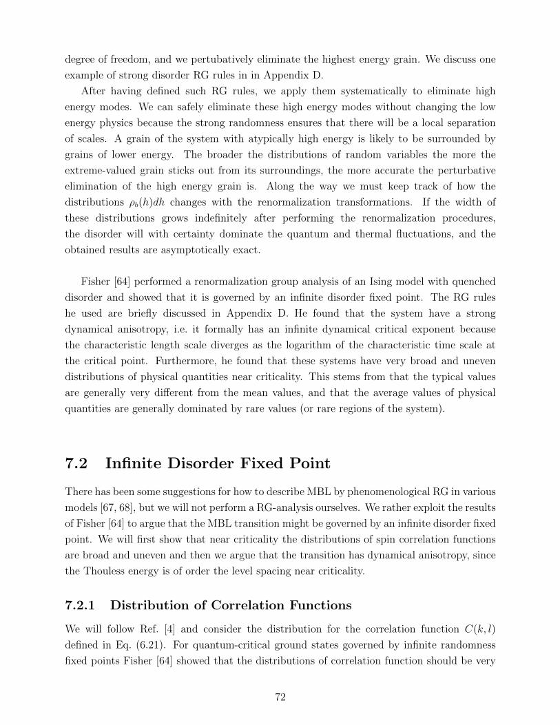
degree of freedom, and we pertubatively eliminate the highest energy grain. We discuss one

example of strong disorder RG rules in in Appendix D.

After having defined such RG rules, we apply them systematically to eliminate high

energy modes. We can safely eliminate these high energy modes without changing the low

energy physics because the strong randomness ensures that there will be a local separation

of scales. A grain of the system with atypically high energy is likely to be surrounded by

grains of lower energy. The broader the distributions of random variables the more the

extreme-valued grain sticks out from its surroundings, the more accurate the perturbative

elimination of the high energy grain is. Along the way we must keep track of how the

distributions ρb(h)dh changes with the renormalization transformations. If the width of

these distributions grows indefinitely after performing the renormalization procedures,

the disorder will with certainty dominate the quantum and thermal fluctuations, and the

obtained results are asymptotically exact.

Fisher [64] performed a renormalization group analysis of an Ising model with quenched

disorder and showed that it is governed by an infinite disorder fixed point. The RG rules

he used are briefly discussed in Appendix D. He found that the system have a strong

dynamical anisotropy, i.e. it formally has an infinite dynamical critical exponent because

the characteristic length scale diverges as the logarithm of the characteristic time scale at

the critical point. Furthermore, he found that these systems have very broad and uneven

distributions of physical quantities near criticality. This stems from that the typical values

are generally very different from the mean values, and that the average values of physical

quantities are generally dominated by rare values (or rare regions of the system).

7.2 Infinite Disorder Fixed Point

There has been some suggestions for how to describe MBL by phenomenological RG in various

models [67, 68], but we will not perform a RG-analysis ourselves. We rather exploit the results

of Fisher [64] to argue that the MBL transition might be governed by an infinite disorder fixed

point. We will first show that near criticality the distributions of spin correlation functions

are broad and uneven and then we argue that the transition has dynamical anisotropy, since

the Thouless energy is of order the level spacing near criticality.

7.2.1 Distribution of Correlation Functions

We will follow Ref. [4] and consider the distribution for the correlation function C(k, l)

defined in Eq. (6.21). For quantum-critical ground states governed by infinite randomness

fixed points Fisher [64] showed that the distributions of correlation function should be very

72

broad and asymmetric, since typical values and mean values differ significantly. So if the

MBL transition is in the infinite disorder universality class, this must also be the case for our

model. We consider

Φk = log|C(k, k +L

2)| (7.3)

We see from Fig. 7.1 that the distribution of Φk is broad in the MBL phase and narrow in the

thermal phase. In the critical region near the phase transition the distribution is asymmetric,

with a fat tail.

Figure 7.1: Distribution of the spin correlation function Φk for systems of size L = 14. For

even smaller disorder strengths the Φ is even more narrowly distributed. Disorder strengths

in legend.

To quantify the width of the distribution and to be able to study how it changes with

system size we need a dimensionless measure of the distribution width. We define η = Φk/Φk

and we consider the standard deviation of η

σL =√η2 − 1

=

√Φ2k − Φk

2

Φk

(7.4)

In the non-localized phase ΦK is roughly constant and the standard deviation of Φk decreases

with increasing system sizes so we expect σL to vanish as L → ∞. In the localized regime

Fisher [64] showed that Φ should grow linearly in L but the standard deviation of Φk only

grows like√L, so σL should vanish for L→∞. At the critical point the typical values of the

correlation function should go as −√L whereas the mean value should be Φk ∼ log(Lφ−2),

73

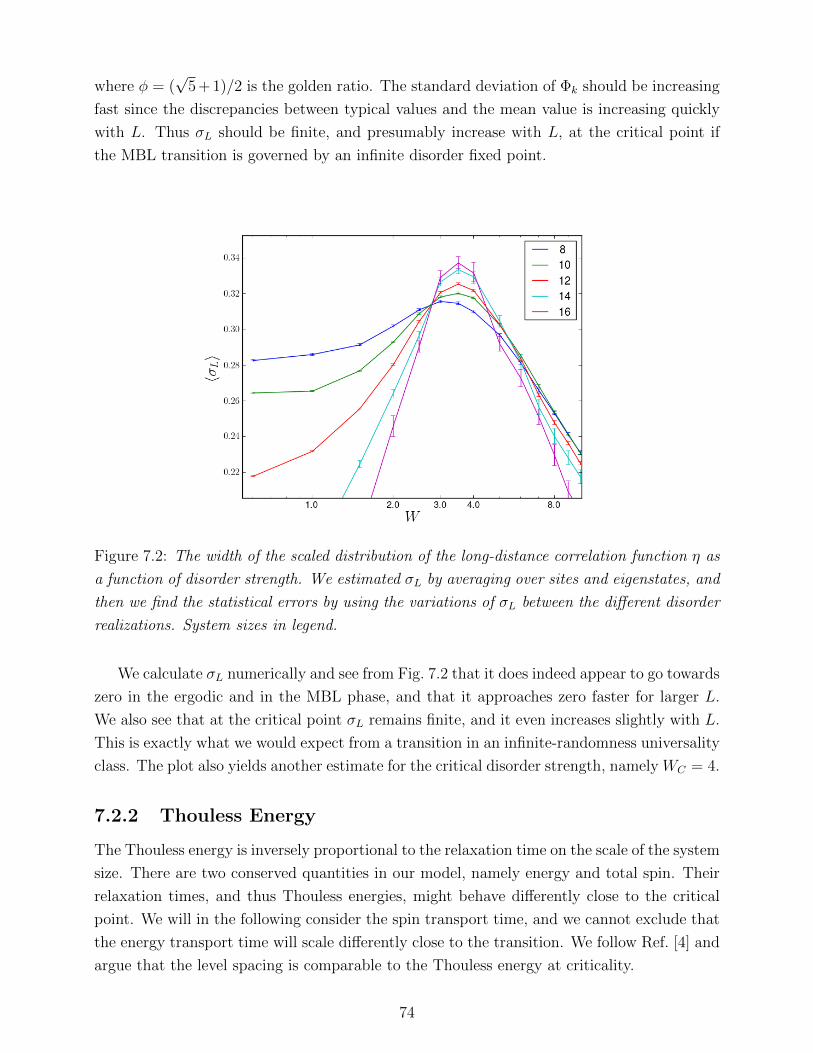
where φ = (√

5 + 1)/2 is the golden ratio. The standard deviation of Φk should be increasing

fast since the discrepancies between typical values and the mean value is increasing quickly

with L. Thus σL should be finite, and presumably increase with L, at the critical point if

the MBL transition is governed by an infinite disorder fixed point.

Figure 7.2: The width of the scaled distribution of the long-distance correlation function η as

a function of disorder strength. We estimated σL by averaging over sites and eigenstates, and

then we find the statistical errors by using the variations of σL between the different disorder

realizations. System sizes in legend.

We calculate σL numerically and see from Fig. 7.2 that it does indeed appear to go towards

zero in the ergodic and in the MBL phase, and that it approaches zero faster for larger L.

We also see that at the critical point σL remains finite, and it even increases slightly with L.

This is exactly what we would expect from a transition in an infinite-randomness universality

class. The plot also yields another estimate for the critical disorder strength, namely WC = 4.

7.2.2 Thouless Energy

The Thouless energy is inversely proportional to the relaxation time on the scale of the system

size. There are two conserved quantities in our model, namely energy and total spin. Their

relaxation times, and thus Thouless energies, might behave differently close to the critical

point. We will in the following consider the spin transport time, and we cannot exclude that

the energy transport time will scale differently close to the transition. We follow Ref. [4] and

argue that the level spacing is comparable to the Thouless energy at criticality.

74

We assume the Thouless energy to be given roughly by the relaxation rate of the spin

density modulation of M as given in Eq. (6.30), and we can think of the Thouless energy

as a measure of how much different eigenstates affect each other. In the thermal phase ET

is large and many states affect each other, whereas in the MBL phase ET is exponentially

small, so different states do not influence each another significantly. We will in the following

argue that the Thouless energy is of the same order of magnitude as the level spacing at the

transition, and this implies that only the states which are adjacent in the energy spectrum

will affect each other near criticality.

Thus a non-zero fraction of the dynamic part of 〈M〉 should be from its matrix elements

between adjacent energy levels, also in the thermodynamic limit.

Continuing our discussion in Sect. 6.5.2; the contribution to the dynamical part of 〈M〉from a given energy eigenstate should be given by

∆Mn = 〈n|M †M |n〉 − |〈n|M |n〉|2 (7.5)

We showed that this appears to approach zero in the MBL phase and remains non-zero in the

thermal phase. In the thermal phase ∆Mn has contributions from matrix elements with many

other eigenstates and ET is a measure of the energy range over which these contributions

occur. We look at contributions to the dynamic part of ∆Mn from the matrix elements

between state n and n± i

Qi = |〈n− i|M |n〉|2 − |〈n|M |n+ i〉|2 (7.6)

We insert a complete set of eigenstates to see that we have

∆Mn =∑m

〈n|M †|m〉〈m|M |n〉 − |〈n|M |n〉|2

=∑i 6=0

|〈n− i|M |n〉|2 − |〈n|M |n+ i〉|2 =∑i 6=0

Qi

(7.7)

We define

Pn =Q1

∆Mn

(7.8)

Where Pn is the fraction of the dynamics which is due to interference between adjacent

energy levels. In the thermal phase we expect matrix elements between many different states

to contribute to the dynamic part of ∆Mn, so many of the Qi’s should contribute significantly.

However in the MBL phase the Thouless energy is exponentially small and therefore none

of the Qi’s give significant contributions to the dynamic part of ∆Mn. In the MBL phase

we have both Q1 and ∆Mn going to zero. Thus both in the MBL and in the thermal phase

we expect Pn to approach zero for increasing system size. If ET is of the same order of

magnitude as δ at the transition, we expect Qi to contribute to ∆Mn only for i = 1 close to

75

the critical point. Thus Pn should be non-zero at the critical point, also when we take the

thermodynamic limit.

Figure 7.3: Fraction of dynamics which comes from adjacent eigenstates as a function of

disorder strength. Average is over eigenstates and disorder realizations. System sizes in

legend.

We see from Fig. 7.3 that both in the MBL and thermal phase 〈Pn〉 appears to be

approaching zero as we increase L. Furthermore we do indeed see a strong peak in 〈Pn〉around the critical point, indicating that the maximal contribution from adjacent states is

near the phase transition. The peaks decrease a little for increasing L but not as much as the

system size is increased, so the results seem to comply with ET ∼ δ scaling at the transition.

If we disregard L = 8, the peaks seems to drift very slightly towards larger W and the peak

appears at W ≈ 2.8 for L = 16, suggesting that the critical disorder strength is WC = 3.

Dynamical Anisotropy

Continuous quantum phase transition generally have some characteristic time scale τC and

characteristic length scale lC which diverge at the critical point. The dynamical critical

exponent z is given by the scaling of τC with lC near the critical point as τC ∼ lzC . In other

words the characteristic time diverges as the z’th power of the characteristic length when we

approach the phase transition.

We know that Anderson localization transition occurs when ET ∼ δ. The single-particle

level spacing for a d-dimensional system of linear size L behaves roughly as δ ∼ L−d and

we therefore have ET ∼ L−d. We have a diverging correlation length ξ and therefore the

76

characteristic length scale of the system equals L. The characteristic time scale is the

Thouless time, which is the inverse of ET . We therefore have τT ∼ Ld scaling at criticality

and the system thus has a dynamic critical exponent which is z = d.

We now assume that the MBL transition occurs when the Thouless energy and the level

spacing are of the same order of magnitude, as we argued above. The level spacing goes

roughly as log(δ) ∼ −Ld. This gives us the scaling log(τT ) ∼ Ld which is characteristic for

infinite critical exponents. We here have the typical length scale related to the logarithm

of the typical time scale and thus a formally infinite dynamical exponent z = ∞. We note

that even for our model with d = 1 this is a stronger divergence of the critical time scale

than what is known from infinite randomness critical points in ground states[64], where

log(τC) ∼ lψC with ψ ≤ 1/2 [64].

7.3 Dynamics & Spectral Functions

In this section we will investigate the long-time dynamics in the thermal phase when we

approach the phase transition. We will show that there can be anomalous diffusion on the

thermal side of the transition and argue that there is a broad critical region. We also further

argue that ET ∼ δ at criticality.

Some recent studies have reported sub-diffusive transport close to the critical point of

the MBL transition [55, 56, 57]. This is believed to be due to so-called “Griffiths effects”

. This is when the low-frequency response is dominated by contributions from rare regions.

In our case it is regions which locally behave as the MBL phase on the thermal side of the

transition. These insulating regions impede the transport but do not prevent thermalization.

Particularly in one dimension this can severely affect the dynamics because the locally

insulating regions can act as bottlenecks [59]. Griffiths effects arise due to regions with

atypical configurations of the quenched randomness.

Griffiths effects were first brought to the fore by Griffiths [58] when considering

thermodynamic and dynamic singularities due to rare regions in disordered systems near

phase transitions.

We assume that the ETH ansatz in Eq. (4.32) describes the matrix elements of some local

observable A, and we show that we can relate g(E, ω) to the dynamics of the system. If we

neglect the variations of the entropy near E=0, it can be shown that g2(ω) is the average

spectral function of A for the states with energy close to zero. We will therefore denote g2(ω)

the spectral function in the following. Our discussion will be similar to the recent work of

77

Abanin, Papic and Serbyn [54]. We consider the following connected correlation function

Fn(t) = 〈n|A(t)A(0)|n〉 − 〈n|A(t)|n〉〈n|A(0)|n〉

=∑m6=n

|〈n|A|m〉|ei(En−Em)t (7.9)

Since we assumed that the ETH ansatz holds for the matrix elements of A we can readily

evaluate the correlation function

Fn(t) =∑m 6=n

g2(E, ω)R2mne

−S(E)eiωt (7.10)

We use that g(E, ω) is a smooth function to argue that R2mn should level out in the sum, and

switch from the summation over the eigenstates to an integral over the density of states as∑m 6=nR

2mn →

∫dEm ρ(Em) =

∫dω e(En+ω), where we also switch integration variable to ω.

This gives

Fn(t) =

∫dω g2(En +

ω

2, ω)eS(En+ω)−S(En+ω

2)e−iωt (7.11)

We are interested in the long-time dynamics of the system so we need to consider small

frequencies, and we therefore Taylor expand the entropy and the spectral function to the

first order about ω = 0 as

S(En + ω)− S(En +ω

2) =

βω

2+O(ω2)

g2(En +ω

2, ω) = g2(En, ω) +

ω

2

dg2(En, ω)

dωO(ω2)

(7.12)

Using this we arrive at

Fn(t) ≈∫dω e−iωte

βω2

[g2(En, ω) +

ω

2

dg2(En, ω)

dω

](7.13)

We also Taylor expand exp(βω/2) = 1 + β2ω/2 +O(ω2). The long-time correlation function

is thus the Fourier transform of g2(En, ω) at small frequencies

Fn(t) ≈∫dω e−iωtg2(En, ω) (7.14)

Since we are in the thermal phase where we have assumed ETH to hold, the dynamics should

be diffusive or super/sub-diffusive. We consider how the correlation function should behave

under diffusive transport. We have the one-dimensional diffusion equation

∂φ

∂t= D

∂2φ

∂x2(7.15)

which is solved by the Green’s function

G(xo, to|x, t) =1√

4πD(t− t0)e− (x−x0)2

2(t−t0) (7.16)

78

Where D is the diffusion constant. We associate our correlation function Fn(t) to the Green’s

function for the diffusion equation G(x0, 0|x0, t). This leads us to expect Fn(t) ∼ |t|−γ, where

γ = 1/2. However if we assume anomalous sub-diffusion† we get γ < 1/2.

We thus assume that Fn(t) describes the diffusive or sub-diffusive transport and Fourier

transform Eq. (7.14) to estimate g2(ω)

g2(ω) =

∫ ∞−∞

dt |t|−γeiωt ∝ ωγ−1 (7.17)

Furthermore we expect the diffusive transport to saturate at a time approximately equal

to the Thouless time τT , since for times longer than τT local excitations explore the entire

system, and the diffusion saturates. We get saturation g2(ω) ∼ K for some constant K for

frequencies ω < ET ; in this region the ETH ansatz reduces to RMT prediction for the matrix

elements. We therefore conjecture the approximate functional form of the spectral function

g2(ω) ≈ K

1 + ( ωET

)1−γ (7.18)

Which encapsulates the diffusive behavior and saturates at frequencies smaller than the

Thouless energy. We have thus showed that we can obtain information about the dynamics

as encoded in Fn(t) by studying the g2(ω), and found an expression for the behavior of

g2(ω) under diffusive transport. We rewrite and modify the ETH ansatz slightly to get an

alternative expression for the spectral function

g2(ω) = eS(E)〈|A2nm|δ(ω − (En − Em))〉 (7.19)

If we broaden the δ-function to be much larger than the level spacing and assume that the

fluctuations R2nm average out, we see that Eq. (7.19) is equivalent to the ETH ansatz in

Eq. (4.32).

†We note that anomalous diffusion is not described by the standard diffusion equation. One of the easiest

way to model anomalous diffusion is to assume a time-dependent diffusivity D(t) = αtα−1D in Eq. (7.15),

where α = γ/2.

79

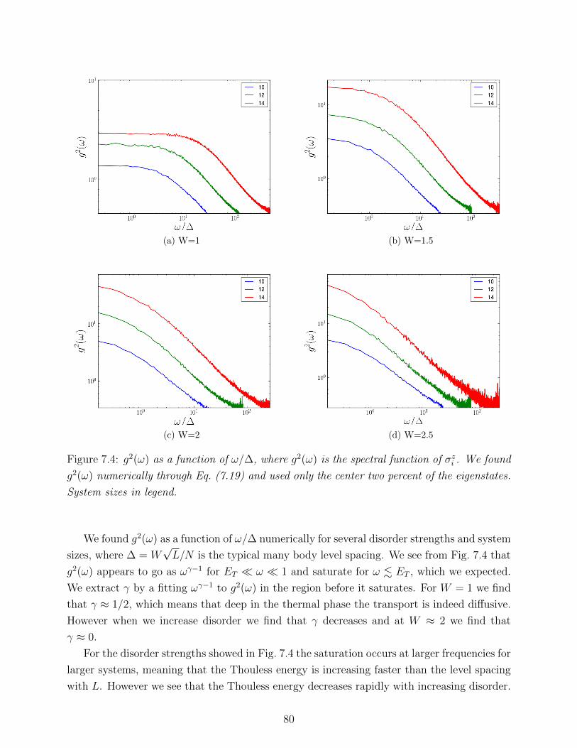
(a) W=1 (b) W=1.5

(c) W=2 (d) W=2.5

Figure 7.4: g2(ω) as a function of ω/∆, where g2(ω) is the spectral function of σzi . We found

g2(ω) numerically through Eq. (7.19) and used only the center two percent of the eigenstates.

System sizes in legend.

We found g2(ω) as a function of ω/∆ numerically for several disorder strengths and system

sizes, where ∆ = W√L/N is the typical many body level spacing. We see from Fig. 7.4 that

g2(ω) appears to go as ωγ−1 for ET ω 1 and saturate for ω . ET , which we expected.

We extract γ by a fitting ωγ−1 to g2(ω) in the region before it saturates. For W = 1 we find

that γ ≈ 1/2, which means that deep in the thermal phase the transport is indeed diffusive.

However when we increase disorder we find that γ decreases and at W ≈ 2 we find that

γ ≈ 0.

For the disorder strengths showed in Fig. 7.4 the saturation occurs at larger frequencies for

larger systems, meaning that the Thouless energy is increasing faster than the level spacing

with L. However we see that the Thouless energy decreases rapidly with increasing disorder.

80

Already for W = 2.5 we see that g2(ω) does not fully saturate, which signifies that ET ∼ δ.

However g2(ω) retains a slight upward curvature through the MBL transition, and is is not

before W > 4 that we see a power law behavior for g2(ω) even for energies smaller than the

level spacing.

We fit the curves in Fig. 7.4 with the functional form of g2(ω) in Eq. (7.18) and use K,

γ and ET as parameters of the fit, and thereby extract the Thouless energy.

Figure 7.5: The Thouless energy divided by level spacing as a function of system size L.

We extracted the Thouless energy by fitting Eq. (7.18) with g2(ω). For disorder larger than

W = 2.5 the Thouless energy is to small to be reliable determined in this way. Disorder

strengths in legend.

We see from Fig. 7.5 that the Thouless energy is comparable to the level spacing in a

broad region before the MBL transition. We have plotted the Thouless energy of a diffusive

system ET ∝ L−2 and see that this seems to be roughly consistent with the data for W = 1.

When we increase the disorder we see that ET/∆ increases slower with L. For disorder

larger than W = 2, the Thouless energy increases only a little faster than the level spacing

with increasing L. This could possibly mean that the Thouless energy in goes as ET ∝ L1γ

with a very small γ. It seems however more natural to interpret this as ET ∝ exp(−κL), for

some sufficiently small κ, similar to in a MBL system. The many-body level spacing scales

roughly as 2−L so we need to have κ . log(2), since ET/∆ is indeed increasing slightly. We

interpret this exponential scaling of ET as a sign of our system entering a critical region

which starts at disorder strength W ≈ 2.

We assume that there is correlation a length ξ(W ) which diverges at MBL transition,

81

since the MBL transition is a continuous phase transition. Thus close to WC it could be the

case that ξ(W ) ≥ L, and when this is the case the system will appear to be at the transition,

since it is to small to capture the delocalized behavior. That is, if we consider a system at

scales smaller than the correlation length, it will appear critical. We see that for disorder

W ≈ 2 the correlation length appears to be larger than L = 14, and therefore g2(ω) can no

longer capture the delocalized behavior of the system.

82

Chapter 8

Summary and Outlook

We have shown the existence of two distinct phases in the random-field Heisenberg model,

namely the thermal phase and the MBL phase. We transition from the thermal to the MBL

phase by increasing the disorder strength W and we found the critical value to be WC =

3.5 ± 1.0. We have distinguished between the phases through the scaling of entanglement

entropy, level statistics, transport properties, participation ratios and whether or not the

system satisfies the ETH.

We can view this transition as an eigenstate phase transition, where the eigenstates

have very different properties in the two phases. Very crudely we say that in the thermal

phase all eigenstates appear the same and in the MBL phase all eigenstates appear different.

What we mean by this is that the all thermal eigenstates within some energy window

should, according to the ETH, reproduce the thermodynamic ensembles at given energy

density, whereas the MBL states are exponentially localized around different basis states

in configuration space. This eigenstate transition is invisible to equilibrium statistical

mechanics, because statistical mechanics averages over many eigenstates and thus washes

out the sharp change in terms of single eigenstates.

The fact that there can exist two distinct phases in closed, strongly interacting, disordered

quantum systems has been well established over the course of the last 10 years. However

not everything about the MBL transition is known. We have argued that the the Thouless

energy is of the order the level spacing at the transition, which implies a formally infinite

dynamical critical exponent. We have also seen that the dynamics can be sub-diffusive in

the thermal phase and signs of a critical region near the phase transition. Furthermore we

discussed the possibility of the MBL transition belonging to the infinite disorder universality

class.

There are some sides of the MBL phase and the MBL transition which we have not

touched upon in this thesis. One of these is localization protected quantum order. It has

83

been shown that individual energy eigenstates of MBL systems can break symmetries or

display topological order in the thermodynamic limit. This can happen at energy densities

where the corresponding thermally equilibrated systems are disordered, and MBL systems

can move between ordered and disordered phases via non-thermodynamic transitions in the

properties of the many-body eigenstates [69, 70].

We have also not properly touched upon multifractality, which is believed to occur near

the phase transition. There have been some studies interpreting the matrix elements of an

observable as the wavefunction of a local excitation and reporting on a strong multifractal

spectrum at the critical point [54, 71].

It would have also been interesting to consider the spreading of entanglement. MBL

systems initially prepared in states with low entanglement have a fast growth of entanglement,

and after some time the entanglement has a slow, logarithmic growth [72]. For an infinite

system the entanglement is expected to grow indefinitely, whereas for a finite system it

saturates to some value, which depends on the system size and should be smaller than in

the thermal phase. This unbounded growth is compatible with the absence of transport, and

it stems from the interaction-induced dephasing involved in the decomposition of the initial

state. This is different from Anderson localization, where the entanglement saturates to a

finite level, also in thermodynamically large systems.

Most of the MBL theory is formulated in terms of exact eigenstates of closed systems.

This is a useful idealization which sheds light on the phenomenology of MBL, but to make

contact with experiments we should presumably consider other approaches and it would

therefore be interesting to consider a MBL system weakly coupled to a heat bath. Such a

system can be studied using spectral functions of local observables, similar to what we did

in Sect. 7.3, since these retain signatures of MBL even when coupled to a heat bath [74].

Furthermore the picture of the MBL transition as an “eigenstate phase transition” has been

critiqued in Ref. [73], where they argue for the possibility that there is an “eigenstate phase

transition” within the MBL phase. That is, they argued through approximately conserved

quasi-local operators that the MBL phase can have eigenstates which satisfies the ETH.

The MBL phase has recently been experimentally observed in a couple of different

systems. In Ref. [6] MBL was observed for interacting fermions in an one-dimensional

optical lattice, where they considered the relaxation dynamics of an initially prepared

charge density wave to identify MBL. Similarly the relaxation dynamics of bosons in two

dimensions has been used to observe the MBL transition in Ref. [8]. They prepared an

out-of-equilibrium density pattern and found evidence for a diverging length scale when

approaching the transition. MBL has also been reported to occur in linear arrays of cold,

trapped atomic ions [7].

There are still many open questions concerning MBL. One interesting issue is if it is

84

possible to have MBL without disorder. There have been some studies arguing for the

existence of translation invariant MBL. In Ref. [75] they found numerical evidence for MBL

in a disorder free Josephson-junction array. Effects similar to MBL have been reported to

occur in a translation invariant systems of hard-core bosons with infinite range and periodic

interactions in Ref. [77], in a system which contains two species of hard-core particles with

very different masses in Ref. [76] and in an exactly soluble model with an extensive number of

conserved quantities in Ref. [78]. In these disorder-free models the systems seem to somehow

generate their own randomness dynamically. Which role disorder plays in MBL is still not

fully understood, and further study of localization of a purely dynamic origin would be

interesting.

It is also not completely understood if it is possible to have mobility edges in MBL system,

i.e. MBL transitions as functions if energy. It was generally believed that MBL systems can

indeed have mobility edges, but in Ref. [79] it was argued that MBL can only occur for lattice

model which are localized at all energies and that previously reported mobility edges cannot

be distinguished from finite-size effects. They argued that local hot thermal spots, which

they denotes “bubbles”, constitute a mechanism for global delocalization.

An effective field theory approach of MBL has also recently been considered in Ref. [80]

where XXZ-chains in the presence of local disorder were considered. It would be interesting

to consider this model (or a similar one) further and possibly us it to identify the universality

class of the MBL transition.

It has recently been shown that spontaneous breaking of time-translation symmetry

can occur in periodically driven MBL systems with discrete time-translation symmetries

[83, 82, 84]. Wilczek [81] considered the possibility of time-crystals, which intriguingly has a

spontaneous breaking of the continuous time-translation symmetry. This was subsequently

proven to be disallowed in equilibrium, but in oscillating quantum systems spontaneous

breaking of time-translation symmetry is possible. After having observed so-called discrete

time-crystals, it would be interesting to consider using this for various quantum information

tasks and also to investigate which role MBL in general could play in realizing quantum

computers.

85

Appendices

86

Appendix A

Consequences of the ETH-ansatz

We will show explicitly that when the ETH ansatz in Eq. (4.32) correctly describes the matrix

elements of observables the systems will be thermal We will also see how fast the discrepancies

between the long time average and the thermodynamic ensemble average vanish when we

increase the size of our system. Given a system fulfilling ETH we consider the canonical

thermal average

〈A〉th =

∑n e−βEnA(En)∑n e−βEn

+∑n

Rnne−βEn

Ze−

S(En)2 g(En, 0)

=

∫∞0dE

∑n δη(E − En)e−βEA(E)∫∞

0dE

∑n δη(E − En)e−βE

+O(e−S2 )

=

∫∞0

dEEeS(E)−βEA(E)∫∞

0dEEeS(E)−βE

+O(e−S2 )

(A.1)

We solve these integral through the saddle point approximation. This demands dS(E)dE

= β,

which we expected since this is how we define temperature in the canonical ensemble, this

also fixes E = Eth. We have S(E) as an extensive quantity which we may write in terms of

the entropy per particle s(e) = S(E,N)/N where e = E/N is the energy per particle. This

gives us N(s(e)− βe) in the exponential. We can now change integration variable to energy

per particle use the standard saddle point approximation which may be stated as∫γ

dzf(z)eλS(z) = F (S(z0))eλS(z0)[f(z0) +O(λ−1)] (A.2)

Where F (S(z)) is some function of the eigenvalues of the Hessian matrix for S(z). This gives

〈A〉th ≈A(Eth) +O(N−1)

1 +O(N−1)+O(e−

S2 ) (A.3)

Since N is large we can Taylor expand the first term to first order to get that it is A(Eth) +

O(N−1).

We can also show explicitly that the second term in Eq. (A.1) is exponentially small

in entropy. However we will simply hold this as obvious, since we know that Rnm and

87

exp(−βEn)/Z are both of order O(1) and g(En, 0) will certainly not be exponentially large.

Therefore the term exp(−S(E)/2) dominate the second term and it goes exponentially fast

to zero. Where we use that we have assumed highly excited states, which implies that the

entropy should be extensive. We thus have

〈A〉th = A(Eth) +O(e−S2 ) +O(N−1) (A.4)

We now study the time-evolution of the expectation value of A

〈A(t)〉 =∑n

|Cn|2(A(En) + g(En, 0)e−S(E)

2 Rnn) +∑n6=m

C∗nCme−i(Em−En)tg(E, ω)e−

S(E)2 Rnm

(A.5)

We then take the infinite-time average

⇒ 〈A(t)〉 =∑n

A(En)|Cn|2 +O(e−S(E)

2 ) (A.6)

We Taylor-expand A(En) about Eth to the second order

〈A(t)〉 = A(Eth) +∑n

[(En − Eth)|Cn|2

dAdE

∣∣∣∣∣Eth

+ (En − Eth)2|Cn|2d2AdE2

∣∣∣∣∣Eth

+O(e−S(E)

2 )]

= A(Eth) + ∆2d2AdE2

∣∣∣∣∣Eth

+O(e−S(E)

2 )

(A.7)

Where we have used that we are concerned with a closed system for which it must hold that

Eth = 〈E〉. We here quantify in terms of the operator A what we mean by demanding the

uncertainty in energy being small, namely ∆2 |A/A′′|. All in all, this leaves us with

〈A(t)〉 = 〈A〉th +O(N−1) +O(∆2) +O(e−S(E)

2 ) (A.8)

We have also shown that the infinite time average equals the ensemble average, and this

follows entirely from the structure of the matrix elements without any assumptions regarding

the initial state, other than that it is away from the edges of the spectrum and that it has

relatively small uncertainty in energy.

88

Appendix B

Calculation of Level Repulsion

We will in the following determine the probability distribution of r(n) as defined in Eq. (6.7).

We consider the statistical probability for r(n) to equal r

P (r) =

⟨δ(r − min∆n,∆n−1

max∆n,∆n−1)

⟩(B.1)

Where the average depends on which statistics En follow. We generally need to use the

joint probability distribution for the eigenvalues to calculate P (r). We consider the cases

when the spectra obeys Poisson and GOE statistics.

Poisson statistics

For the Poisson statistics P (r) can be easily evaluated analytically since the levels are

completely randomly distributed and therefore the level spacings must also follow the Poisson

distribution

PPoisson(r) =1

δ2

∫ ∞0

d∆n

∫ ∞0

d∆n−1δ(r −min∆n,∆n−1max∆n,∆n−1

)e−∆nδ e−

∆n−1δ (B.2)

We split the integral into the two parts; one where ∆n−1 < ∆n and the other where ∆n−1 >

∆n.

PPoisson(r) =1

δ2

∫ ∞0

d∆n−1

∫ ∆n−1

0

d∆nδ(r −∆n

∆n−1

)e−∆nδ e−

∆n−1δ

+1

δ2

∫ ∞0

d∆n

∫ ∆n

0

d∆n−1δ(r −∆n−1

∆n

)e−∆nδ e−

∆n−1δ

=2

δ2

∫ ∞0

d∆n

∫ ∆n

0

d∆n−1 ∆nδ(∆nr −∆n−1)e−∆nδ e−

∆n−1δ

=2

δ2

∫ ∞0

d∆n ∆ne−∆n(1+r)

δ

(B.3)

89

Where we used that we know from definition that r ≤ 1. The last integral is simply solved

through the Gamma-function.

Γ(z) =

∫ ∞0

dx xz−1e−x

⇒ Γ(2) =

∫ ∞0

dx xe−x =(1 + r)2

δ2

∫ ∞0

dx′ x′e−x′ (1+r)

δ

(B.4)

We know that Γ(n) = (n− 1)! ∀n ∈ IN, and we thus arrive at

PPoisson(r) =2

(1 + r)2(B.5)

Now we can find the expectation value of r(n) for a spectrum obeying Poisson statistics

〈r〉Poisson =

∫ 1

0

dr rPPoisson

=

∫ 1

0

dr2r

(1 + r)2

=[ 2

1 + r+ 2 ln(1 + r)

]1

0= 2 ln(2)− 1 ∼= 0.39

(B.6)

Gaussian Orthogonal Ensemble Statistics

Within GOE it is somewhat more involved to calculate the probability distribution of r(n)

exactly, due to the level repulsion. In the Poisson-case the statistics of En’s and ∆n’s are the

same so it was straightforward to evaluate the distribution. For the GOE we need the joint

probability distribution from Eq. (3.14), but its not tractable to calculate this exactly so we

assume a 3x3-matrix and use the PDF on this matrix. Hopefully this will mimic the behavior

for arbitrary N well, in the same way that the Wigner surmise was a good approximation

for large N . We now venture to find the GOE distribution of r(n)

PGOE(r) ∝∫ ∞−∞

dEn−1

∫ ∞En−1

dEn

∫ En−1

−∞dEn−2 δ(r − min∆n,∆n−1

max∆n,∆n−1)

× |En − En−1||En − En−2||En−1 − En−2|e−E2n4 e−

E2n−14 e−

E2n−24

(B.7)

Here we once again consider separately the cases where ∆n ≶ ∆n−1 and exploit that the

energies are ordered, i.e. En ≥ En−1 ≥ En−2 which renders the absolute value signs obsolete

PGOE(r) ∝∫ ∞−∞

dEn−1

∫ ∞En−1

dEn

∫ En−1

−∞dEn−2 δ(r − (En − En−1)

(En−1 − En−2))

× (En − En−1)(En − En−2)(En−1 − En−2) e−(E2n+E2

n−1+E2n−2)

4

+ C

∫ ∞−∞

dEn−1

∫ ∞En−1

dEn

∫ En−1

−∞dEn−2 δ(r − (En−1 − En−2),

(En − En−1))

× (En − En−1)(En − En−2)(En−1 − En−2) e−(E2n+E2

n−1+E2n−2)

4

(B.8)

90

We now change variables to

x = En−1 − En−2 ∈ [0,∞)

y = En − En−1 ∈ [0,∞)

En−1 ∈ (−∞,∞)

(B.9)

For the exponents we then get

E2n + E2

n−1 + E2n−2 = (En−1 + y)2 + (x− En−1)2 + E2

n−1

= 3(E2n−1 +

1

3(x− y))2 − 1

3(x− y)2 + x2 + y2

(B.10)

We now shift the limits of integration in the integral over En−1 by 13(x− y) which does not

cause any problem since our function goes exponentially fast to zero when the arguments go

to infinity. This yields

PGOE(r) ∝∫ ∞−∞

dEn−1

∫ ∞0

dx

∫ ∞0

dy δ(yr − x)y2x(x+ y) e−(x2+y2− 1

3 (x−y)2)

4 e−π3E2

n−14

∝∫ ∞

0

dx

∫ ∞0

dy δ(yr − x)y2x(x+ y) e−(x2+y2− 1

3 (x−y)2)

4

∝∫ ∞

0

dy y4(r + r2) e−((1+r+r2)y2

6

(B.11)

We use the known definite integral∫ ∞0

dxx2ne−αx2

=(2n)!

n!22n+1

√π

α2n+1(B.12)

to get

PGOE(r) = Kr + r2

(1 + r + r2)52

(B.13)

We now find our normalization constant through demanding that our distribution for r musr

to be normalized to unity

N∫ 1

0

drr + r2

(1 + r + r2)52

= N 4

27!

= 1 (B.14)

Where we evaluated the integral in Mathematica. Now we can readily evaluate the

expectation value of r(n) for a GOE spectrum∫ 1

0

r PGOE(r)dr =

∫ 1

0

dr27r

4

r + r2

(1 + r + r2)52

=[− x3 + 15x2 + 12x+ 8

2(x2 + x+ 1)32

]1

0= 4− 2

√(3) ∼= 0.53

(B.15)

Where we once again used Mathematica. We have thereby showed that⟨r(n)⟩Poisson

∼= 0.39

and⟨r(n)⟩GOE

∼= 0.53. The GOE prediction is something of an approximation but we find

numerically that it is rather accurate. It is easy to find this numerically by considering a

large ensemble of Gaussian orthogonal random matrices and estimating the average value of

r(n) over this ensemble.

91

Appendix C

Kubo Formula for Conductivity

Tensor

Using linear response and in particular the Kubo formula we will deduce an expression for

the DC part of the electric conductivity tensor. We know that the total current J (ω) can be

expressed as the linear response to an electric field E(ω) as J (ω) = σ(ω)E(ω), and we have

the Kubo formula for the conductivity

σ(ω) =1

Ω

∫ ∞0

dte−iωt∫ β

0

dλ⟨J(−iλ)J(t)

⟩(C.1)

where the current operator J is in the Heisenberg picture, i.e. J(t) = eiHtJe−iHt where H is

the unperturbed (without electric field) Hamiltonian. The volume of the system is denoted

Ω and⟨· · ·⟩

= trZ−1e−βH · · · denotes the thermal average. We go through the integrals

σ(ω) =1

ZΩ

∫ ∞0

dte−iωt∫ β

0

dλ∑n

〈n|e−βHeλHJe−λHeiHtJe−iHt|n〉

=1

ZΩ

∑nm

e−βEn∫ ∞

0

dte−iωtei(Em−En)t

∫ β

0

dλeλ(En−Em)〈n|J |m〉〈m|J |n〉(C.2)

Where |n〉 are the eigenstates of the unperturbed Hamiltonian and we inserted a complete

set of states. Now will we add an infinitesimal convergence factor ηt in the exponential. This

corresponds to an adiabatic switching-on of the electromagnetic field at t = −∞. The limit

η → 0 should be taken later

σ(ω) =1

ZΩ

∑nm

e−βEn1− eβ(En−Em)

En − Em

∫ ∞0

dtei(Em−En−ω+iη)t〈n|J |m〉〈m|J |n〉

=1

ZΩ

∑nm

i〈n|J |m〉〈m|J |n〉Em − En − ω + iη

e−βEn − e−βEmEn − Em

(C.3)

We are only interested in the DC-current and we will therefore be taking the limit of frequency

going to zero later. We thus only need to consider the real part of the conductivity. We will

92

make use of the following identity

1

ω ± iη= P 1

ω± iπδη(ω) (C.4)

Where P1/ω denotes the principal value of 1/ω and the delta function has been regularized,

but in the limit η → 0 it goes to the standard Dirac delta function.

<σ(ω) =∑nm

〈n|J |m〉〈m|J |n〉ZΩ

e−βEn − e−βEmEn − Em

<iP 1

Em − En − ω− πδη(Em − En − ω)

=π

ZΩ

∑nm

〈n|J |m〉〈m|J |n〉e−βEn − e−βEmEm − En

δη(Em − En − ω)

=π

ZΩ

∑nm

〈n|J |m〉〈m|J |n〉e−βEn 1− e−βω

ωδη(Em − En − ω)

(C.5)

We now take the limit of frequency going to zero. Where we Taylor expand

limω→0

1− e−βω

ω= lim

ω→0

1− (1− βω + 12β2ω2 + . . .)

ω= β (C.6)

We then arrive at

<σ(ω → 0) =πβ

ZΩ

∑nm

〈n|J |m〉〈m|J |n〉e−βEnδη(Em − En) (C.7)

We finally use that the total current J is given as the sum over all local currents

J =∑r

Jr =∑r

er (C.8)

This yields our final result

<σ(ω → 0) =πβ

ZΩ

∑r′r

∑nm

〈n|Jr+r′|m〉〈m|Jr|n〉e−βEnδη(Em − En) (C.9)

93

Appendix D

RG Rules for Random

transverse-Field Ising Model

We will here review the renormalization group transformation, as suggested by Fisher [64],

to the transverse field Ising Hamiltonian with quenched randomness. The Hamiltonian for

the model is

H = −∑j

JjSzjS

zj+1 −

1

2

∑j

hjSxj (D.1)

Where the interaction strengths Jj’s are drawn independently from a distribution π0(J)dJ

and the transverse fields hj from ρo(h)dh, where both the hj’s and the Jj’s are positive.

The renormalization transformation consists of the following steps; we find the largest

interaction term or field in the system with strength Ω = Ω0 ≡ maxJj, hj and decimate

this away to get rid of the high energy information and focus on the desired low energy

physics. There are two possibilities:

• If Ω = Jj we make the approximation that the two spins Sj and Sj+1 are rigidly locked

together as a spin cluster with an effective field h ≈ hjhj+1/Ω and effective magnetic

moment g = gj + gj+1 = 2, obtained from lowest order perturbation theory in hj/Jj.

• If Ω = hj we simply eliminate this site and get an effective interaction strength J =

JjJj−1/Ω between the remaining nearest neighbor sites j + 1 and j − 1.

This procedure is to be iterated. At each step both J and h is necessarily smaller than Ω, so

when we iterate the maximal energy scale will gradually decrease. We need to keep track of

the distributions πΩ(J) and ρΩ(h, g) at each step. Fisher showed that these distributions will

broaden exponentially, which implies that the perturbative decimation process gets better

and better.

94

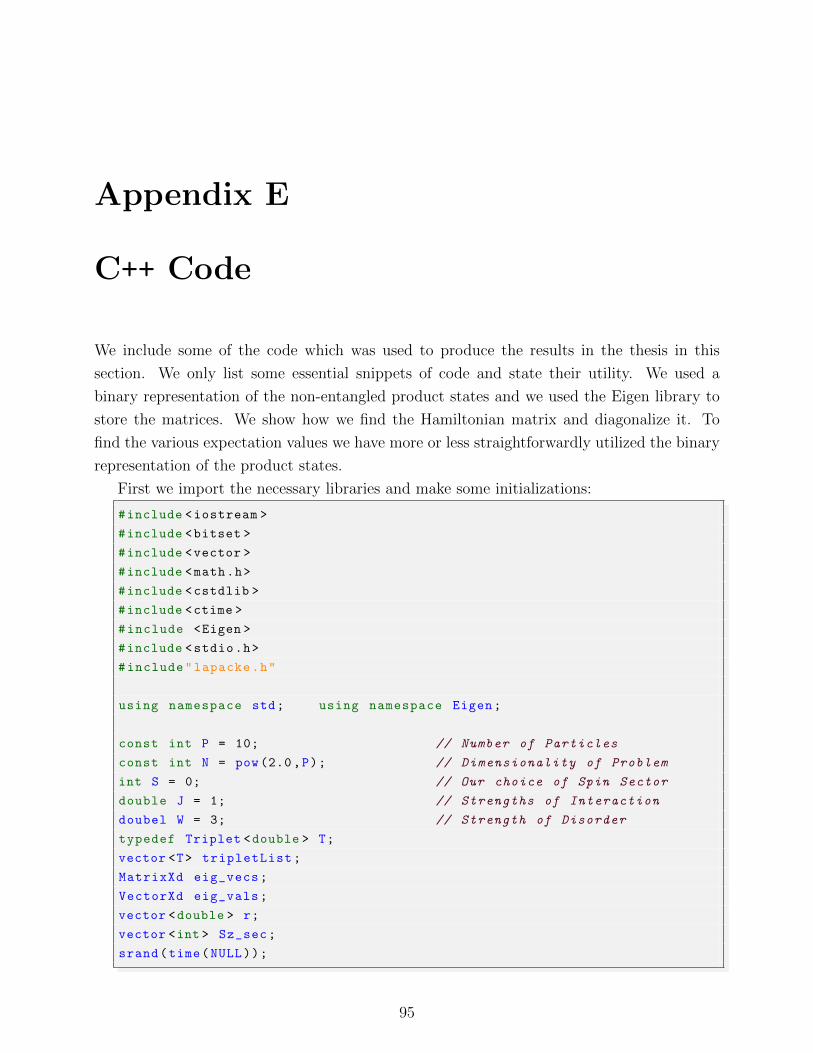
Appendix E

C++ Code

We include some of the code which was used to produce the results in the thesis in this

section. We only list some essential snippets of code and state their utility. We used a

binary representation of the non-entangled product states and we used the Eigen library to

store the matrices. We show how we find the Hamiltonian matrix and diagonalize it. To

find the various expectation values we have more or less straightforwardly utilized the binary

representation of the product states.

First we import the necessary libraries and make some initializations:

#include <iostream >

#include <bitset >

#include <vector >

#include <math.h>

#include <cstdlib >

#include <ctime >

#include <Eigen >

#include <stdio.h>

#include"lapacke.h"

using namespace std; using namespace Eigen;

const int P = 10; // Number of Particles

const int N = pow(2.0,P); // Dimensionality of Problem

int S = 0; // Our choice of Spin Sector

double J = 1; // Strengths of Interaction

doubel W = 3; // Strength of Disorder

typedef Triplet <double > T;

vector <T> tripletList;

MatrixXd eig_vecs;

VectorXd eig_vals;

vector <double > r;

vector <int > Sz_sec;

srand(time(NULL));

95

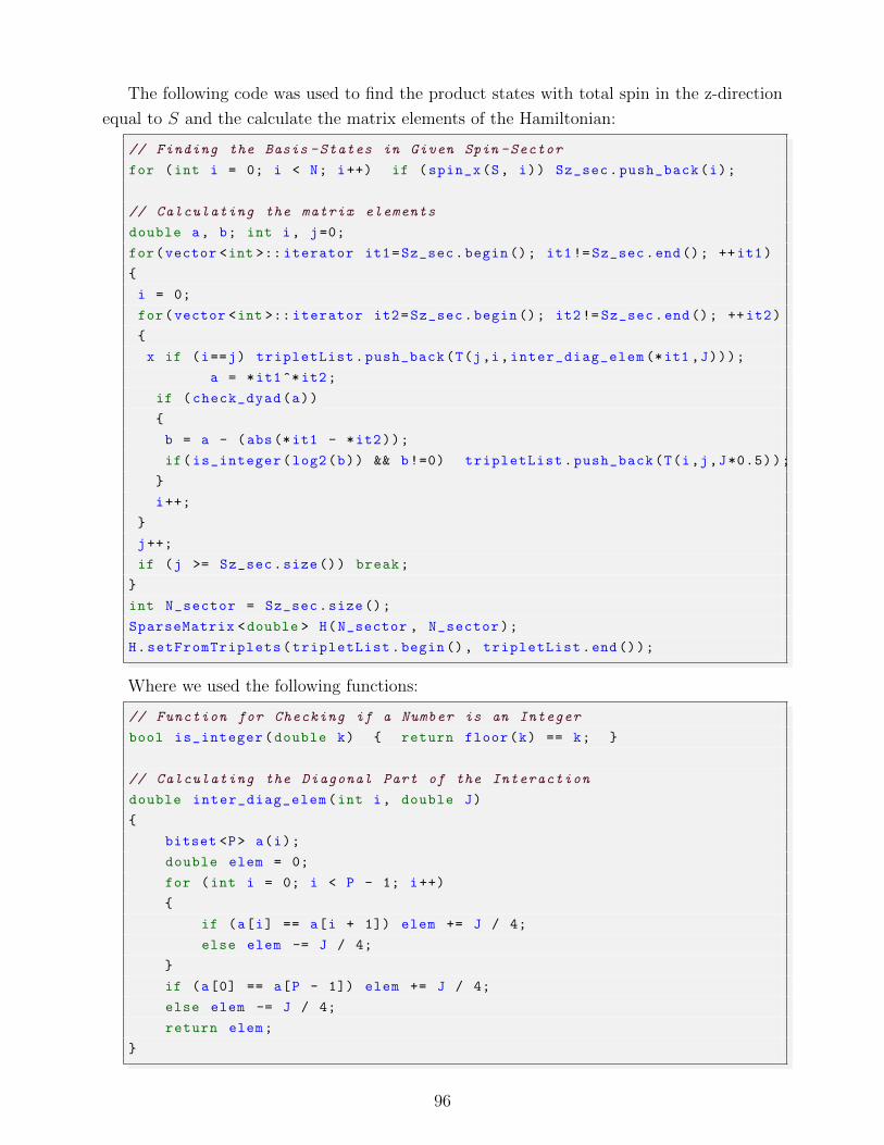
The following code was used to find the product states with total spin in the z-direction

equal to S and the calculate the matrix elements of the Hamiltonian:

// Finding the Basis -States in Given Spin -Sector

for (int i = 0; i < N; i++) if (spin_x(S, i)) Sz_sec.push_back(i);

// Calculating the matrix elements

double a, b; int i, j=0;

for(vector <int >:: iterator it1=Sz_sec.begin(); it1!= Sz_sec.end(); ++it1)

i = 0;

for(vector <int >:: iterator it2=Sz_sec.begin(); it2!= Sz_sec.end(); ++it2)

x if (i==j) tripletList.push_back(T(j,i,inter_diag_elem (*it1 ,J)));

a = *it1^*it2;

if (check_dyad(a))

b = a - (abs(*it1 - *it2));

if(is_integer(log2(b)) && b!=0) tripletList.push_back(T(i,j,J*0.5));

i++;

j++;

if (j >= Sz_sec.size()) break;

int N_sector = Sz_sec.size();

SparseMatrix <double > H(N_sector , N_sector);

H.setFromTriplets(tripletList.begin (), tripletList.end());

Where we used the following functions:

// Function for Checking if a Number is an Integer

bool is_integer(double k) return floor(k) == k;

// Calculating the Diagonal Part of the Interaction

double inter_diag_elem(int i, double J)

bitset <P> a(i);

double elem = 0;

for (int i = 0; i < P - 1; i++)

if (a[i] == a[i + 1]) elem += J / 4;

else elem -= J / 4;

if (a[0] == a[P - 1]) elem += J / 4;

else elem -= J / 4;

return elem;

96

// Checking if a binary Number has two adjacent 1’s and the rest 0’s

bool check_dyad(int a)

bitset <P> b(a);

int dyad = 0;

int count = 0;

int last_bit = 1;

for (int i = 0; i < P; i++) if (b[i] == 1) count += 1;

if (count == 2)

for (int i = 0; i < P; i++)

if (b[i] == 1 && i != P - 1)

if (b[i + 1] == 1)

dyad = 1;

break;

if (b[0] == 1 && b[P - 1] == 1) dyad = 1;

return dyad;

// Checking if Product State has total Spin equal to given S

bool spin_tot(int S, int i)

bitset <P> spins(i);

bool is_spin_tot = 0;

int count = 0;

for (int i = 0; i < P; i++)

if (spins[i] == 1) count ++;

else count --;

if (count == S) is_spin_tot = 1;

return is_spin_tot;

We then calculate the disorder part of the Hamiltonian for each disorder realization as:

// Adding the random Fields

r = gen_ran_vec(W, (double)rand());

for(int i=0; i<N_sector; i++) A.coeffRef(i,i)+= rand_elem(r,Sz_sec[i]);

97

Where we used the following functions:

// Generating the random Part of the i’th diagonal Element

double rand_elem(vector <double > ran_vec , int i)

bitset <P> spins(i);

double elem = 0;

for (int i = 0; i < P; i++)

if (spins[i]) elem += ran_vec[i]*0.5;

else elem -= ran_vec[i]*0.5;

return elem;

// Generating a Vector of uniformly distributed random Numbers on [-W,W]

vector <double > gen_ran_vec(double W, double seed)

vector <double > R;

srand(seed);

for(int i=0; i<N; i++) R.push_back (2*W*(rand()/double(RAND_MAX) -0.5));

return R;

We diagonalize the matrix using the dsyev routine from LAPACK:

// Diagonalizing

int LDA = N_sector;

int n = N_sector; lda = LDA , info , lw;

double wk;

double* work;

double w[N_sector ];

double* L = A.data();

lw= -1;

LAPACK_dsyev ((char*)"Vectors",(char*)"Upper",&n,L,&lda ,w,&wk ,&lw ,&info);

lw = (int)wkopt;

work = (double *) malloc( lwork*sizeof(double) );

LAPACK_dsyev ((char*)"Vectors",(char*)"Upper",&n,L,&lda ,w,work ,&lw ,&info);

if( info > 0 )

printf( "The algorithm failed to compute eigenvalues .\n" );

exit( 1 );

free( (void*)work );

eig_vals = Map <VectorXd >(w,N_sector);

eig_vecs = Map <MatrixXd >(L,N_sector ,N_sector);

98

Bibliography

[1] P. W. Anderson, Phys. Rev. 109, 1492 (1958)

Absence of Diffusion in Certain Random Lattices

[2] D. M. Basko, I. L. Aleiner, B. L. Altshuler, Annals of Physics 321, 1126 (2006)

Metal-insulator Transition in a weakly interacting Many-electron System with localized

Single-particle States

[3] I. V. Gornyi, A. D. Mirlin, D. G. Polyakov, Phys. Rev. Lett. 95, 206603, (2005=

Interacting Electrons in Disordered Wires: Anderson Localization and Low-T Transport

[4] A. Pal, D. A. Huse, Phys. Rev. B 82, 174411 (2010)

The many-body Localization Phase Transition

[5] B. Bauer, C. Nayak, J. Stat. Mech. P09005 (2013)

Area Laws in a Many-body localized State and its Implications for topological Order

[6] M. Schreiber, S. S. Hodgman, P. Bordia, H. P. Luschen, M. H. Fischer, R. Vosk, E.

Altman, U. Schneider, I. Bloch, Science 349, 842 (2015)

Observation of Many-body Localization of interacting Fermions in a quasi-random

optical Lattice

[7] P. W. Hess, P. Becker, H. B. Kaplan, A. Kyprianidis, A. C. Lee, B. Neyenhuis, G. Pagano,

P. Richerme, C. Senko, J. Smith, W. L. Tan, J. Zhang, C. Monroe, arXiv:1704.02439

Non-thermalization in trapped Atomic Ion Spin Chains

[8] J. Choi, S. Hild, J. Zeiher, P. Schauß, A. Rubio-Abadal, T. Yefsah, V. Khemani, D. A.

Huse, I. Bloch, C. Gross, Science 352, 1547 (2016)

Exploring the Many-body Localization Transition in two Dimensions

[9] M. Srednicki, Phys. Rev. E 50, 888 (1994)

Chaos and Thermalization

[10] M. Srednicki, J. Phys. A 32, 1163 (1999)

The Approach to Thermalization in quantized chaotic Systems

99

[11] J. M. Deutsch, Phys. Rev. A 43, 2046 (1991)

Quantum statistical Mechanics in a closed System

[12] A. Einstein, Annalen der Physik 322 (8): 549–560

Uber die von der molekularkinetischen Theorie der Warme geforderte Bewegung von in

ruhenden Flussigkeiten suspendierten Teilchen

[13] G. Feher, E. A. Gere, R. C. Fletcher, Phys. Rev. 100, 1784, (1955)

Exchange Effects in Spin Resonance of Impurity Atoms in Silicon

[14] G. Feher, E. A. Gere, Phys. Rev. 114, 1245, (1959)

Electron Spin Resonance Experiments on Donors in Silicon. II. Electron Spin Relaxation

Effects

[15] G. Feher, Phys. Rev. 114, 1219, (1959)

Electron Spin Resonance Experiments on Donors in Silicon. I. Electronic Structure of

Donors by the Electron Nuclear Double Resonance Technique

[16] D. J. Thouless, J. T. Edwards, J. Phys. C: Solid State Phys., Vol. 5, 1572 (1972)

Numerical Studies of Localization in Disordered Systems

[17] E. Abrahams, P. W. Anderson, D. C. Licciardello, and T. V. Ramakrishnan

Phys. Rev. Lett. 42, 673 (1979)

Scaling Theory of Localization: Absence of Quantum Diffusion in Two Dimensions

[18] F. J. Wegner, Z Physik B 25: 327,

Electrons in disordered Systems. Scaling near the Mobility edge

[19] F. Evers, A. D. Mirlin, Rev. Mod. Phys. 80, 1355 (2008)

Anderson Transitions

[20] A. D. Mirlin, Lectures International School ”Enrico Fermi” on New Directions in

Quantum Chaos (1999),

Statistics of Energy Levels and Eigenfunctions in disordered and chaotic Systems:

Supersymmetry Approach

[21] K. B. Efetov, Int.J.Mod.Phys.B24:1756-1788, (2010)

Anderson Localization and Supersymmetry

[22] N. F. Mott, Phil. Mag.19 (160):835-852 (1969)

Conduction in Non-crystalline Materials

[23] E. P. Wigner, Annals of Mathematics. 62 (3): 548–564

Characteristic vectors of bordered Matrices with Infinite Dimensions

100

[24] E. P. Wigner, Ann. Math 67, 325 (1958)

On the Distribution of the Roots of Certain Symmetric Matrices

[25] F.J Dyson, Journal of Mathematical Physics 3, 140 (1962)

Statistical Theory of the Energy Levels of Complex Systems

[26] L. Zhang, V. Khemani, D. A. Huse, Phys. Rev. B 94, 224202, (2016)

A Floquet Model for the Many-Body Localization Transition

[27] J. Isserlis, Biometrika. 11: 185–190 (1916)

On a Formula for the Product-moment Coefficient of any Order of a normal Frequency

Distribution in any Number of Variables

[28] A. Polkovnikov, K. Sengupta, A. Silva, M. Vengalattore Rev.Mod.Phys.83:863, (2011)

Nonequilibrium Dynamics of closed interacting Quantum Systems

[29] M. V. Berry, J. Phys. A: Math, Gen., Vol. 10, No. 12, (1977)

Regular and irregular Semiclassical Wavefunctions

[30] O. Bohigas, M. J. Giannoni, C. Schmit, Phys. Rev. Lett. 52, 1, (1984)

Characterization of Chaotic Quantum Spectra and Universality of Level Fluctuation

Laws

[31] M.V. Berry, M. Tabor, Proc. R. Soc. Lond. A. 356, 375-394 (1977)

Level Clustering in Regular Spectrum

[32] H. Stockmann, Scholarpedia, 5(10):10243 (2010)

[33] M. V. Berry, Physica Scripta, Vol. 40, 335-336, (1989)

Quantum Chaology, not Quantum Chaos

[34] O. Bohigas, M. Giannoni, Lecture Notes in Physics, vol 209. Springer, Berlin, Heidelberg

Chaotic Motion and random Matrix Theories

[35] E. Wigner, Phys. Rev. 40, 749, (1932)

On the Quantum Correction for Thermodynamic Equilibrium

[36] M. Rigol, V. Dunjko, M. Olshanii, Nature 452, 854-858 (2008)

Thermalization and its Mechanism for generic isolated Quantum Systems

[37] J. Frohlich, T. Spencer Comm. Math. Phys. 88, 2, 151-184. (1983)

Absence of Diffusion in the Anderson tight Binding Model for large Disorder or low

Energy

[38] F. Evers, A. D. Mirlin, Phys. Rev. Lett. 84, 3690 (2000)

Fluctuations of the Inverse Participation Ratio at the Anderson Transition

101

[39] T. Guhr, Axel Mueller-Groeling, H. A. Weidenmueller Phys.Rept.299:189-425,1998

Random Matrix Theory in Quantum Physics: Common Concepts

[40] Y. Alhassid, Rev. Mod. Phys. 72, 895 (2000)

The statistical Theory of Quantum Dots

[41] P. Ponte, Z. Papic, F. Huveneers, D. A. Abanin, Phys. Rev. Lett. 114, 140401 (2015)

Many-body Localization in periodically driven Systems

[42] D. Page Phys.Rev.Lett.71:1291-1294,1993

Average Entropy of a Subsystem

[43] S. Sen Phys.Rev.Lett. 77 1-3 (1996)

Average Entropy of a Subsystem

[44] T. A. Brody, J. Flores, J. B. French, P. A. Mello, A. Pandey, S. S. M. Wong

Rev. Mod. Phys. 53, 385 – 1 July 1981

Random-Matrix Physics: Spectrum and Strength Fluctuations

[45] T. Tao, V. Vu 2011 2011

Random Matrices: Universal Properties of Eigenvectors

[46] V. Khemani, F. Pollmann, S. L. Sondhi Phys. Rev. Lett. 116, 247204 (2016)

Obtaining highly-excited Eigenstates of Many-body localized Hamiltonians by the Density

Matrix Renormalization Group

[47] C. Zhang, F. Pollmann, S. L. Sondhi, R. Moessner, arXiv:1608.06411

Density-Matrix Renormalization Group study of Many-Body Localization in Floquet

Eigenstates

[48] D. A. Huse, R. Nandkishore, V. Oganesyan Phys. Rev. B 90, 174202 (2014)

Phenomenology of fully Many-body-localized Systems

[49] J. Z. Imbrie, Jour. Stat. Phys. 163:998-1048 (2016)

On Many-Body Localization for Quantum Spin Chains

[50] V. Ros, M. Mueller, A. Scardicchio, Nuclear Physics, Section B (2015), pp. 420-465

Integrals of Motion in the Many-Body localized Phase

[51] J. Z. Imbrie, V. Ros, A. Scardicchio, arXiv:1609.08076 (2016)

Review: Local Integrals of Motion in Many-Body Localized systems

[52] F. Izrailev, Phys. Rep. 196, 299–392 (1990)

Simple Models of Quantum Chaos: Spectrum and Eigenfunctions

102

[53] D. A. Huse, V. Oganesyan, Phys. Rev. B 75, 155111 (2007)

Localization of interacting Fermions at high Temperature

[54] M. Serbyn, Z. Papic, D. A. Abanin, arXiv:1610.02389 (2016)

Thouless Energy and Multifractality across the Many-body Localization Transition

[55] M. Znidaric, A. Scardicchio, V. K. Varma, Phys. Rev. Lett. 117, 040601 (2016)

Diffusive and Subdiffusive Spin Transport in the Ergodic Phase of a Many-body localizable

System

[56] D. J. Luitz, N. Laflorencie, F. Alet, Phys. Rev. B 93, 060201 (2016)

Extended slow dynamical Regime prefiguring the Many-body Localization Transition

[57] K. Agarwal, S. Gopalakrishnan, M. Knap, M. Mueller, E. Demler, Phys. Rev. Lett. 114,

160401 (2015)

Anomalous dDffusion and Griffiths Effects near the Many-body Localization Transition

[58] R. B. Griffiths, Phys. Rev. Lett. 23, 17, (1969)

Nonanalytic Behavior Above the Critical Point in a Random Ising Ferromagnet

[59] K. Agarwal, E. Altman, E. Demler, S. Gopalakrishnan, D. A. Huse, M. Knap, Annalen

Der Physik 1600326 (2017)

Rare Region Effects and Dynamics near the Many-body Localization Transition

[60] M. Gell-Mann and F. E. Low, Phys. Rev. 95, 1300, (1954)

Quantum Electrodynamics at small Distances

[61] L. P. Kadanoff, Physics Vol. 2, No. 6, pp. 263-272, (1966)

Scaling Laws for Ising Models near TC

[62] K. G. Wilson, Phys. Rev. B 4, 3174, (1971)

Renormalization Group and Critical Phenomena. I. Renormalization Group and the

Kadanoff Scaling Picture

[63] C. Dasgupta, S. Ma, Phys. Rev. B 22, 1305, (1980)

Low-Temperature Properties of the random Heisenberg Antiferromagnetic Chain

[64] D. S. Fisher, Phys. Rev. Lett. 69, 534, (1992)

Random transverse Field Ising Spin Chains

[65] D. S. Fisher, Phys. Rev. B 50, 3799, (1994)

Random antiferromagnetic Quantum Spin Chains

[66] D. S. Fisher, Phys. Rev. B 51, 6411, (1995)

Critical Behavior of random transverse-Field Ising Spin Chains

103

[67] R. Vosk, E. Altman, Phys. Rev. Lett. 110, 067204, (2013

Many-body Localization in one Dimension as a dynamical Renormalization Group fixed

Point

[68] L. Zhang, B. Zhao, T. Devakul, D. A. Huse, Phys. Rev. B 93, 224201 (2016)

Many-body Localization Phase Transition: A simplified strong-randomness approximate

Renormalization Group

[69] Y. Bahri, R. Vosk, E. Altman, A. Vishwanath, arXiv:1307.4092

Localization and Topology protected Quantum Coherence at the Edge of ’hot’ Matter

[70] D, A. Huse, R. Nandkishore, V. Oganesyan, A. Pal, S. L. Sondhi, Phys. Rev. B 88,

014206 (2013)

Localization protected Quantum Order

[71] C. Monthus, J. Stat. Mech. 073301, (2016)

Many-Body-Localization Transition: Strong multifractality Spectrum for Matrix

Elements of local Operators

[72] J. H. Bardarson, F. Pollmann, J. E. Moore, Phys. Rev. Lett. 109, 017202 (2012)

Unbounded Growth of Entanglement in Models of Many-body Localization

[73] A. Chandran, A. Pal, C.R. Laumann, A. Scardicchio, Phys. Rev. B 94, 144203 (2016)

Many-body Localization beyond Eigenstates in all Dimensions

[74] R. Nandkishore, S. Gopalakrishnan,Annalen der Physik, 1521-3889 (2016)

General Theory of many-body localized Systems coupled to Baths

[75] M. Pino, B. L. Altshuler, L. B. Ioffe, arXiv:1501.03853

Non-ergodic metallic and insulating Phases of Josephson Junction Chains

[76] M. Schiulaz, A. Silva, M. Muller, Phys. Rev. B 91, 184202 (2015) Dynamics in many-body

localized Quantum Systems without Disorder

[77] R. Mondaini, Z. Cai, arXiv:1705.00627

Many-body Self-Localization in a Translation-invariant Hamiltonian

[78] A. Smith, J. Knolle, D. L. Kovrizhin, R. Moessner, arXiv:1701.04748

Disorder-free Localization

[79] W. de Roeck, F, Huveneers, M. Muller, M.Schiulaz, Phys. Rev. B 93, 014203 (2016)

Absence of many-body Mobility Edges

[80] A. Altland, T. Micklitz, Phys. Rev. Lett. 118, 127202 (2017)

Effective Field Theory Approach to Many-body Localization

104

[81] F. Wilczek, arXiv:1202.2539

Quantum Time-Crystals

[82] N.Y. Yao, A.C. Potter, I.-D. Potirniche, A. Vishwanath, Phys. Rev. Lett. 118, 030401,

(2017)

Discrete Time Crystals: Rigidity, Criticality, and Realizations

[83] D. V. Else, B.Bauer, C. Nayak, Phys. Rev. Lett. 117, 090402 (2016)

Floquet Time Crystals

[84] J. Zhang, P. W. Hess, A. Kyprianidis, P. Becker, A. Lee, J. Smith, G. Pagano, I.-D.

Potirniche, A. C. Potter, A. Vishwanath, N. Y. Yao, C. Monroe, arXiv:1609.08684

Observation of a Discrete Time Crystal

105