manual for colloid chemistry practical...
TRANSCRIPT

Manual for
Colloid Chemistry Practical Course
Pharmacy program 2017/2018
1st semester, 2
nd year
Edited by Márta Berka, Levente Novák,
Mónika Kéri, Dávid Nagy and Zoltán Nagy
University of Debrecen
Department of Physical Chemistry
http://kolloid.unideb.hu/en/practice/
OPERATION OF THE LABORATORY................................................................................2
EXPERIMENTS..............................................................................................................8 1. Rheological characterization of concentrated emulsions (creams) ................................8
2. Measurement of surface tension of solutions by Du Nouy tensiometer ....................... 15 3. Polymer’s relative molecular masses from viscosity measurements ............................ 21
4. Adsorption from solution ........................................................................................... 25 5. Solubilization ............................................................................................................. 31
6 Determination of size distribution of a sedimenting suspension ................................. 35 7. Characterization of substances of different rheological properties by Brookfield DV-
II+ rotational viscosimeter ......................................................................................... 40 8. Steric and electrostatic stabilization mechanisms of colloidal dispersions................... 44
9. Determination of the critical micelle concentration of SDS ........................................ 48 Appendix ....................................................................................................................... 52

2
OPERATION OF THE LABORATORY
THE COURSE
In the seven-week period assigned to the Colloid Chemistry Practical Course, six
experiments have to be performed compulsorily, which are designed to be completed in
four hours respectively. Each of the practices should be finished and the results should be
evaluated in the laboratory. By the end of each lab session you must hand-in a report from the
actual practice (the requirements how to write a report is described later). All experiments are
preceded by a short written test. The short test consists of two questions: the first one is
randomly chosen from the 8 equations below:
Kelvin equation
Einstein-Sokes equation
Gibbs equation
Langmuir isotherm
Gouy-Chapman equation
Stern equation
The two equivalent definitions of surface tension
Equation of the osmotic pressure
For each definition or equation the meaning of the symbols and the units of measurement must
also be present.
The second question is related to the actual practice. You will receive a mark for each short
test and another mark for each report. The average of short test marks and report marks will
be calculated, your final mark will be given by the 2 to 1 weighted average of report marks
and short test marks.
A student can’t have more than two failed marks (1) from the short test results and from the
lab report results, respectively, in order to succsessfully accomplish the subject. One failed
mark from lab reports can be corrected once during the semester, if a calculation error,
plotting mistake or inappropriate conclusion is the reason of the unaccepted mark. The
correction should be performed and the corrected lab report should be re-submitted until the
end of the last practice week.
ATTENDANCE
The Colloid Chemistry laboratory is open from 14:00 to 18:00 on Monday and from 8:00 to
12:.30 on Tuesday and Wednesday. You must arrive on time. Coats and bags should be left in

3
the corridor of the laboratory. The department does not accept responsibility for personal
values (money, jewels, mobile phone, etc) left in the corridor; you should keep them with
you.
Do not leave valuable items in this area!
If you are absent from a practical class (e.g. you are ill), you should report it to the
administration (room D205, Mihály Szatmári) at the earliest opportunity to see whether the
missed experiment(s) can be re-scheduled for an alternative date. Lack of attendance without
good reason will result in a mark of zero.
LABORATORY STAFF
The academic staff member with overall responsibility for the Colloid Chemistry Practical
Course is Prof. István Bányai (room D201). The Laboratory Managers are Mónika Kéri
(Phone: 22385, room D202) on Monday and Levente Novák on Tuesday and Wednesday
(Phone: 22437, room D205), the Technician in charge of the laboratory is Mihály Szatmári
(room D205).
EXPERIMENT BENCHES
Each experiment has a bench assigned to it containing the apparatus and chemicals required
for the particular experiment, except some chemicals or tools that are given by the
Technician. As you will be doing a different experiment each week, it is essential that all the
glassware involved are washed up by the end of a lab session first with tap water and then
with distilled water and left clean in the correct cupboard for the next group’s use, the
following week.
PRE-LABORATORY WORK
You must prepare pre-laboratory work before coming to the laboratory. A brief outline of the
theory of the actual experiment should be written. (Usually it is enough to summarize the
most important definitions, equations, relations, etc. in a half page extent). It should be
followed by the description of the expereminent, the detailed recipe that you have to follow to
perform the experiment. On arrival in the laboratory you must show this work to a
Demonstrator and get him/her to sign it. Failure to carry out the pre-laboratory work will
result in the loss of marks. Pre-laboratory work should be carried out in your laboratory
notebook.
4
ASSESSMENT
Your report should be organised into the following sections: Theory, Experimental, Results &
Discussion and Conclusion.
The aspects taken into account for assessing your reports are the following:
• theoretical preparation, experimental skill, the quality of your data;
• the correct processing of data (e.g.correctness in calculations, accuracy in plotting graphs,
inclusion of the appropriate units, labelling of axes, estimation of experimental uncertainties,
etc.);
• correct answers to questions, the conclusion, the overall coherence of the report.
Failure to hand in work on time without good reason will result in downgrading. Exceptions
will only be made if you have previously agreed with the academic staff member in charge of
the laboratory (or have reported an illness to administration). If you get a “fail” (1) mark due
to calculation errors or an inappropriate conclusion in your report, there is a second chance
(only once in the course!) to correct the mistakes. In this case next week when you receive the
report, you should bring back the corrected one until the end of that week (Friday, 12:00). The
best mark you can get is “average” (3).
Final marks will be calculated from the marks of the written short tests weighted with a factor
of one and those from the reports weighted with a factor of two:
final mark = (average of tests + 2 × average of reports) / 3
The calculated final mark will be rounded to the closest integer.
PLAGIARISM
Plagiarism means trying to pass off someone else’s work other than your own. The University
takes very serious measures against students who have commited plagiarism in any context.
This does not mean that you cannot discuss your laboratory work with other students.
However, you can use only those primary data and other results in your report that you have
measured yourself. If a student is found to be committing plagiarism, he or she will receive
zero mark for the actual practice (when calculating your average the sum of the marks won’t
grow, but 1 will be added to the divider).

5
LABORATORY NOTES
One of the objectives of the laboratory teaching is to introduce you to methods of recording
results in a short and logical fashion. The ability to keep an accurate record of your laboratory
work is of principal importance since your lab notes will be used as the basis for your lab
report. You can print the theory part and/or the tables of the given experiment from this
manual and you can put them together in your laboratory notebook or in your folder.
It should become standard practice to record everything relevant directly into your laboratory
notebook. This means you should record weights, data, calculations, rough graphs, reaction
schemes and comments. Do not use scraps of paper with the idea of copying them more
neatly later into your notebook. You should record your notes in ink, not pencil. Every page
should have a clear heading which should include your name, the title of the experiment and
the date at which it was carried out. The record of each experiment should begin with a brief
statement of the experiment to be performed, and a brief plan of the experimental procedure.
This should be done before you come to the lab. You can plot data manually on a mm scale
paper or you can use database management systems like Microsoft Excel. In the latter case all
the plotted graphs should be printed and attached to your report. The most important part of
your report is the conclusion. First you should esteem the correctness and reliability of your
results. (Did you get what you expected?) You should compare your results with literature
data. You can find literature data on the internet or you can ask the supervisor/demonstrator
for them. If the difference is significant, you should try to give explanations, possible reasons
to it. Your laboratory notebook must be signed and dated by the demonstrator or superviser
when you have finished the experiment.
DAMAGE, REPARATIONS
Purchase of broken glassware, reparation of lost or defective utensils are at the charge of
those who mishandled them. A written report form will be filled and signed by the person
responsible for the damage and one of the supervisors. Reparation fee can be paid by cheques
issued by the Department.
SAFETY INFORMATION
Emergency telephone numbers: First aid medical doctor number: 23009; Receptionist: 22300

6
There are First Aid Boxes in each Teaching Laboratory. In the event of a minor accident call
the staff. External Numbers: Fire 9-105, Police 9-107, Ambulance 9-104
FIRE ALARMS
The alarms sound if a sensor detects flame, heat or smoke or if the break-glass alarm button is
activated. Before activating the alarm you should size up the situation to avoid unnecessary
fire alarms. In case of fire first you should inform the staff in charge, after that follow their
instructions.
If you are in a practical class when the alarms sound, spend a few seconds for making your
experiment safe, then leave the building by the nearest marked exit. Do not use the elevators!
Do not attempt to enter the building until you have been told it is safe to do so!
LABORATORY SAFETY
Whilst working in the laboratory, it is your responsibility, by law:
• To take reasonable care for your own health and safety and for that of others in the
laboratory
• To co-operate in matters of health and safety.
• Not to interfere with, or damage, any equipment provided for the purpose of protecting
health and safety.
SAFETY DATA SHEETS
Before you commence any practical work you must familiarise yourself with the chemical
hazards present in the experiment. No practical work can be undertaken without the
presence of at least one staff member in the laboratory. If you have any queries or
concerns about health and safety in the Teaching Laboratories you should direct these to the
Departmental Safety Adviser.
EMERGENCY EQUIPMENT
You should make yourself familiar with the location of fire extinguishers and fire blankets.
Training in the use of this equipment is given at the beginning of the year. A safety shower is
located by the main door to the lab.
SAFETY PRECAUTIONS
Dress like a chemist. Wear clothing in the laboratory that will provide the maximum body
coverage. When carrying out experimental work you MUST wear a fastened lab coat. In case
of a large chemical spill on your body or clothes, remove contaminated clothing to prevent

7
further reaction with the skin. Every student has to have own safety glasses and to wear them
when it is neccessary.
Eating and drinking is strictly prohibited. This includes chewing gum. Keep long hair tied
back and ensure that long or large necklaces are safely tucked away. Mobile phones personal
stereos etc. must be switched off when entering the laboratory. Anything that interferes with
your ability to hear what is going on in the laboratory is a potential hazard. You are strongly
advised not to wear contact lenses in the laboratory, even under safety glasses. After reading
any warnings and recommendations, use all chemicals carefully whenever possible. Dispose
solvents properly. Immediately return any chemicals you have used to the shelves for other
students to use.
Keep your work area tidy and clean up any spills, including water, on the floor.
Report all accidents and dangerous incidents, no matter how trivial they may seem
Wash your hands carefully when you leave.
Work defensively!

8
EXPERIMENTS
1. Rheological characterization of concentrated emulsions (creams)
Theory
Rheology is the science of flow and deformation of body that describes the interrelation
between force, deformation and time. Rheology is applicable to all materials, from gases to
solids. Viscosity is the measure of the internal friction of a fluid. This friction becomes
apparent when a layer of fluid is made to move in relation to another layer. The greater the
friction, the greater the amount of force is required to cause this movement, which is called
“shear”. Shearing occurs whenever the fluid is physically moved or distributed, as in pouring,
spreading, spraying, mixing, etc. Highly viscous fluids, therefore, require more force to move
than less viscous materials.
The viscosity of a fluid is a measure of its resistance to gradual deformation by shear stress.
Viscosity is due to friction between neighboring parcels of the fluid that are moving at
different velocities. The velocity gradient is the measure of the speed at which the
intermediate layers move with respect to each other. It is also called “shear rate”. This will be
symbolized as “D” in subsequent discussions. Its unit is reciprocal second, s-1
. The force per
unit area required to produce the shearing action is referred to as “shear stress” and will be
symbolized by “”. Its unit of measurement is N/m2 (Newton per square meter). Using these
simplified terms, viscosity may be defined mathematically by this formula:
shear stress τη=viscosity= =
shear rate D The fundamental unit of viscosity measurement is Pas, Pascal-
seconds. A material requiring a shear stress of one Newton per square meter to produce a
shear rate of one reciprocal second has a viscosity of one Pas. (You will encounter viscosity
measurements in “centipoise” (cP) , but these are not units of the International System, SI;
one Pascal-second is equal to ten poise; one milli-Pascal-second is equal to one centipoise.)
Newton assumed that all materials have, at a given temperature, a viscosity that is
independent of the shear rate. In other words twice the force would move the fluid twice as
fast.
In rheology fluids are categorized in three groups:
Newtonian fluids
Non-Newtonian, time independent fluids

9
Non-Newtonian, time dependent fluids
The sub-categories and examples to the flow- and viscosity curves of these fluids is
summarized in Figure 1. The detailed descripton of the categories can be found in the
Appendix at the end of this supplementary material.
Figure 1. Flow and viscosity curves of newtonian and non-newtonian time-independent
fluids
1. ideal (newtonian), 2. shear thinning or pseudoplastic, 3. shear thickening or dilatant, 4.
ideal plastic (Bingham type), 5. plastic (pseudo-plastic type), 6. plastic (dilatant type)
What happens when the element of time is considered? This question leads us to the
examination of “thixotropy” and “rheopexy”.
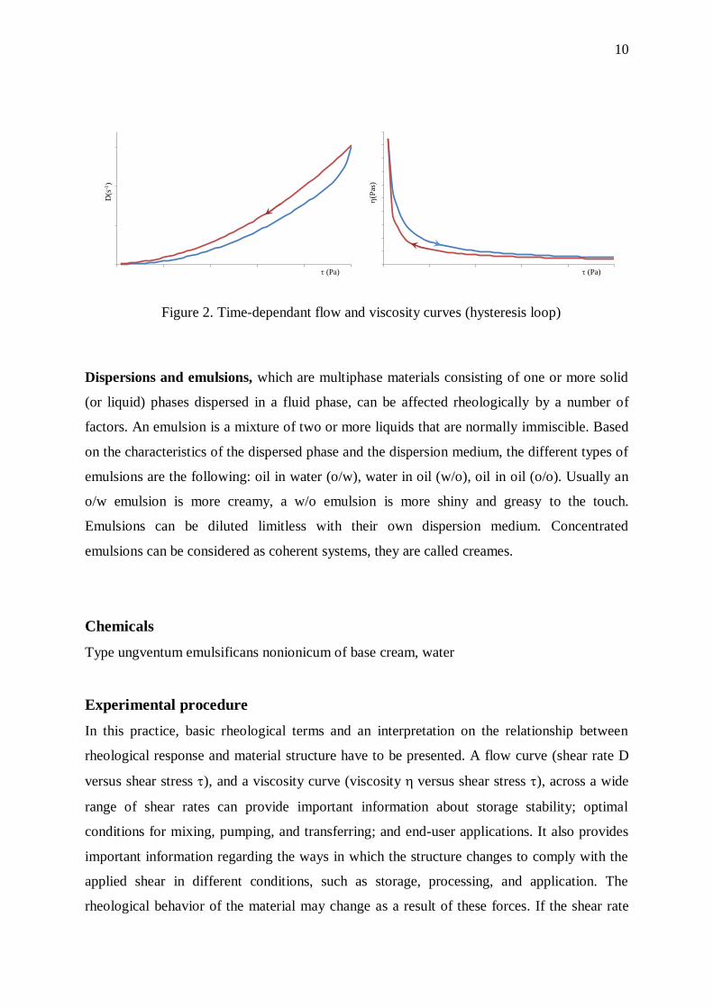
Thixotropic. A thixotropic fluid decreases in viscosity with time, while it is subjected to
constant shearing, as you can find out from Figure2. Rheopectic. This is essentially the
opposite of thixotropic behaviour, in that the fluid’s viscosity increases with time as it is
sheared at a constant rate. See Figure 1. Both thixotropy and rheopexy may occur in
combination with any of previously discussed flow behaviors, or only at certain shear rates.
The time element is extremely variable; under conditions of constant shear, some fluids will
reach their final viscosity in a few seconds, while others may take up to several days.
Rheopectic fluids are rarely encountered. Thixotropy is frequently observed in materials such
as greases, heavy printing inks, and paints. When subjected to varying rates of shear, a
thixotropic fluid will react as illustrated in Figure 2. A plot of shear stress versus shear rate
was made increased to a certain value, then immediately decreased to the starting point. Note
that the “up“ and “down“ curves do not coincide. This “hysteresis loop” is caused by the
decrease in the fluid’s viscosity with increasing time of shearing (Figure 2.). Such effects may
or may not be reversible; some thixotropic fluids, if allowed to stand undisturbed for a while,
will regain their initial viscosity, while others never will.
(Pa)0
D(s
-1)
(Pa)0
D(s
-1)
(Pa)0
D(s
-1)
1
2
3
4
5
6
(Pa)0
h(P
as)
1
2
3
4
5
6
10
Figure 2. Time-dependant flow and viscosity curves (hysteresis loop)
Dispersions and emulsions, which are multiphase materials consisting of one or more solid
(or liquid) phases dispersed in a fluid phase, can be affected rheologically by a number of
factors. An emulsion is a mixture of two or more liquids that are normally immiscible. Based
on the characteristics of the dispersed phase and the dispersion medium, the different types of
emulsions are the following: oil in water (o/w), water in oil (w/o), oil in oil (o/o). Usually an
o/w emulsion is more creamy, a w/o emulsion is more shiny and greasy to the touch.
Emulsions can be diluted limitless with their own dispersion medium. Concentrated
emulsions can be considered as coherent systems, they are called creames.
Chemicals
Type ungventum emulsificans nonionicum of base cream, water
Experimental procedure
In this practice, basic rheological terms and an interpretation on the relationship between
rheological response and material structure have to be presented. A flow curve (shear rate D
versus shear stress ), and a viscosity curve (viscosity hversus shear stress ), across a wide
range of shear rates can provide important information about storage stability; optimal
conditions for mixing, pumping, and transferring; and end-user applications. It also provides
important information regarding the ways in which the structure changes to comply with the
applied shear in different conditions, such as storage, processing, and application. The
rheological behavior of the material may change as a result of these forces. If the shear rate
(Pa)
D(s
-1)
(Pa)
h(P
as)

11
changes during an application, the internal structure of the sample will change and the change
in stress or viscosity can then be seen.
Apparatus
Rheometer LV (Brookfield torque range appropriate for measuring low viscosity materials;
100% torque = 673.7 dyne cm; dial reading viscometer with electronic drive), beaker, glass
rod, spatula
The original Brookfield Dial Reading Viscometer is the lab standard used around the world. Easy
speed control with convenient adjustable rectangular switch is on its side. The pointer can be
stopped with a toggle behind the motor. Viscometers are supplied with a standard spindle set (LV-
1 through LV-4)
Put 150 cm3 of cream (ointment or paste) into the measuring container by avoiding the
formation of air bubbles or other inhomogenity. Screw the appropriate spindle and observe the
operation of the rheometer (spindle must rotate centered). When attaching a spindle,
remember that it has a left-hand thread and must be screwed firmly to the coupling (for this
operation always ask for the help of the supervisors). After attachment do not hit the spindle
against the side of the sample container since this can damage the shaft alignment. When
conducting an original test, the best method for spindle and speed selection is trial and error.
The goal is to obtain a viscometer dial or display reading between 10 and 100 remembering
that accuracy improves as the reading approaches 100. If the reading is over 100, select a
slower speed and/or a smaller spindle. Conversely, if the reading is under 10, select a higher
speed and/or a larger spindle. When conducting multiple tests, the same spindle/speed
combination should be used for all tests. The spindle should be immersed up to the middle of
the indentation in the shaft. We recommend inserting the spindle in a different portion of the
sample than the one intended for measurement. The spindle may then be moved horizontally
to the center of the sample container.
12
1. Immerse the spindle into the sample, and turn the rectangular screw on maximum
speed (RPM = 60, the actual speed is shown on the top of the screw), and allow it to
run for 5 minutes then let it run at minimum speed (RPM = 6) until a constant reading
is obtained (or for about 15 minutes). (Homogenization) For measurement use every
speed for 30 s.
2. Start the run with 6 RPM and read and write the value of display after 30 s running.
3. Increase the speed of rotation without stopping the motor and read the display again as
before. If there is no dial or readable display or it is less than 5%, change spindle or
speed. Repeat the measurement decreasing the speed from 60 RPM to 6 RPM, too.
4. After the measurement at all 4 speeds there and back, dilute the emulsion with 5 cm3
water and homogenize thoroughly with a glass rod. Repeat the measurement
procedure from point 1 to point 3.
Two more repetitions are needed following the instructions of point 4. (In total 4 times
5 cm3 deionized water will be added to the cream.)
Tabulate the data and plot rheology (D) and viscosity (h) curves.
Calculation of the results
Viscosity: h (Pas) = z × 1 1
Shear stress: N/m2) = h× D = z×D×1 2
Shear rate: D(s-1
) = RPM×constant
Viscometer torque: displayed in %
Centimetre–gram–second system (CGS) is a variant of the metric system of physical units. In rheology it is still widespread; Viscosity: 1 mPas = 1 cP Shear stress: 1 N/m
2 = 10 dyne/cm
2 Torque:
1 Nm = 107 dyne cm.
RPM D (s-1
)
6 0.1
12 0.2
30 0.5
60 1
z (insrtument constant)
RPM/spindle no 4 3 2 1
6 1000 200 50 10
12 500 100 25 5
30 200 40 10 2
60 100 20 5 1
13
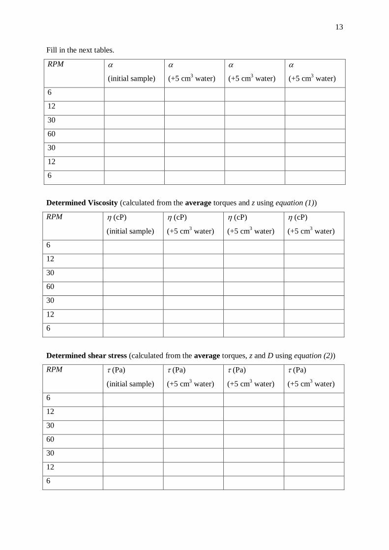
Fill in the next tables.
RPM
(initial sample)
(+5 cm3 water)
(+5 cm3 water)
(+5 cm3 water)
6
12
30
60
30
12
6
Determined Viscosity (calculated from the average torques and z using equation (1))
RPM h (cP)
(initial sample)
h(cP)
(+5 cm3 water)
h(cP)
(+5 cm3 water)
h(cP)
(+5 cm3 water)
6
12
30
60
30
12
6
Determined shear stress (calculated from the average torques, z and D using equation (2))
RPM (Pa)
(initial sample)
(Pa)
(+5 cm3 water)
(Pa)
(+5 cm3 water)
(Pa)
(+5 cm3 water)
6
12
30
60
30
12
6

14
Plot the flow (D) and viscosity (h) curves. Compare your 2 figures to Figure 1 and
determine the rheology class of cream. Explain how and why the , h∞ and hysteresis loop
change with dilution of the cream.
Discuss the results.
Rheology and viscosity curves at different dilution of creams.
(This is only illustration, your results may differ from it depending on the temperature and the
properties of the studied cream)
Review questions
Definition of viscosity. Rheological classification of materials, with their rheology and
viscosity curves. Hysteresis loop.
0
20
40
60
80
100
120
140
0.0 1.0 2.0 3.0 4.0 5.0 6.0 7.0 8.0
, Pa
D, s-1
0ml
5ml
10ml
15ml
added water
víz,ml
0.0
0.1
0.2
0.3
0.0 1.0 2.0 3.0 4.0 5.0 6.0 7.0 8.0
, Pah
, P
as
0ml
5ml
10ml
15ml
added water
víz,ml
15
2. Measurement of surface tension of solutions by Du Nouy tensiometer
Theory
The molecules at the surface of a liquid are subjected to an unbalanced force of molecular
attraction as the molecules of the liquid tend to pull those at the surface inward while the
vapor does not have as strong an attraction. This unbalance causes liquids to tend to maintain
the smallest surface possible. The magnitude of this force is called the surface tension.When
this lowest possible energetic state is achieved the surface tension acts to hold the surface
together where the force is parallel to the surface. The symbol for surface tension is
"gamma". Conventionally the tension between the liquid and the atmosphere is called surface
tension while the tension between one liquid and another is called interfacial tension.
The specific surface free energy or surface tension of surface is equal to the expenditure of
work required to increase the net area of surface isothermally and reversibly way by unit of
area, in J/m2 (Joule per square meter); if the increase in the surface area is accomplished by
moving a unit length of line segment in a direction perpendicular to itself, is equal to the
force, or “tension”, opposing the moving of the line segment. Accordingly, it is usually
expressed in units of N m-1
(Newton per meter). Surface may be a free surface (exposed to air
or vapor or vacuum) or an interface with another liquid or solid. In the event that the surface
is an interface, this quantity is called interface tension. The value of surface tension is
dependent on the nature of the liquid and also on the temperature (see Eötvös and Ramsay
empirical rule). The temperature during the measurement of surface tension must be kept
constant. It is found that the surface tensions of solutions are generally different from those of
the corresponding pure solvents. It has also been found that solutes whose addition results in a
decrease in surface tension tend to be enriched in the surface regions (positive surface
concentration). The migration of solute either toward or away from the surface is always such
as to make the surface tension of the solution (and thus the free energy of the system) lower
than it would be if the concentration of solute were uniform throughout (surface concentration
equal to zero). Equilibrium is reached when the tendency for free-energy decrease due to
lowering surface tension is balanced by the opposing tendency for free-energy increase due to
increasing nonuniformity of solute concentration near to the surface.
A surface-active molecule, also called a surface active agent or surfactant, possesses
approximately an equal ratio between the polar and nonpolar portions of the molecule. When
such a molecule is placed in an oil-water system, the polar group(s) are attracted to or oriented

16
toward the water, and the nonpolar group(s) are oriented toward the oil. This orientation of
amphiphilic molecules is described by Hardy-Harkins principle of continuity. The surfactant
is adsorbed or oriented in this manner, consequently lowering interfacial tension between the
oil and water phase. When a surfactant is placed in a water system, it is enriched at the surface
and lowers the surface tension between the water and air. When it is placed in a mixture of
solid and liquid, it is enriched on the surface of the solid and lowers the interfacial tension
between the solid and the liquid. Since the surfactant is adsorbed at the surface, it is logical
that the concentration of surfactant at the surface would be greater than the concentration in
the bulk solution. Mathematically such a relationship has been derived by Willard Gibbs. It
relates lowering of surface tension to excess concentration of surfactant at the surface.
The Gibbs equation can be written as follows:
1
ln
d
RT d c
(1)
where c is the concentration (in mol m-3
) in the solution, T (K) the absolute temperature, R the
gas constant (8.314 JK-1
mol-1
), (Nm-1
) the surface tension and c (mol m2) is the surface
excess concentration. It follows from Equation 1 that c is positive if d/dc is negative, that is
the surface tension decreases with increasing solute concentration. On the basis of
experimental surface tension vs. solute concentration function the d/dc can be determined
and the c =f (c) adsorption isotherm (Eq. 2) can be calculated.
bc
bc
1 (2a)
b
1cc (2b)
where c is the bulk concentration of the analyte, b is a constant and is the saturation
(maximum) surface excess concentration.
The area (m) occupied per molecule is determined as: A
mN
1
where NA is the
Avogadro’s number (6×10²³
mol-1
). The m for alcohols are about 0.22 nm2 and for carboxylic
acids about 0.25 nm2 extrapolated from the liquid condensed regions and m are about 0.20
nm2
extrapolated from the solid regions of two-dimensional isotherm of monolayer,
idependent of both the length of the hydrocarbon chain and the nature of the head.
Apparatus
Du Nouy tensiometer (this is a highly sensitive microbalance – a delicate instrument and you
should use care when working with it), beakers, volumetric flask, pipettes
17
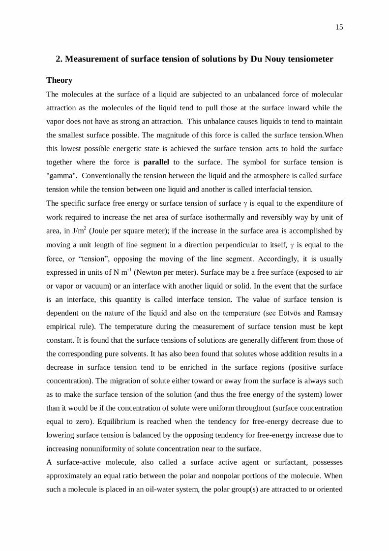
Du Nouy tensiometer
Chemicals
Deionized water, aqueous solution of alcohol or organic acids.
Experimental procedure
This tensiometer is capable of measuring the surface tension of liquids with the du Nouy ring.
The du Nouy tensiometer consists of a platinum-iridium ring supported by a stirrup attached
to a torsion balance. The force that is just requiring breaking the ring free of the liquid/liquid
or liquid/air interface is proportional to the surface tension. The surface tension is displayed
in mN/m, accurate to 0.1 mN/m.
Attach the ring to the balance. Fill the test vessel with deionized water, and suspend the ring
in the liquid and zero the instrument with the ring below the surface of the liquid. (For the
first measurements ask for help from the supervisors). If you are making a surface tension
measurement, begin to lower the platform that the wessel (petri dish) is on and add tension to
the ring to maintain the ring in position until the ring breaks free of the liquid. Read off
measurement when surface breaks. Then repeat the measurement as before. The ring can be
cleaned with distilled water. Care must be taken not to touch or bent the ring with the
fingers! The measured (apparent) surface tension for deionized water (water measured) slightly
differs from literature water surface tension (water) due to the different geometry of the rings.
You can obtain the corrected values by multiplying the measured surface tensions with a
correction factor=water/water measured. The correction factor is normally close to one.
Prepare 0.0, 0.10, 0.20, 0.50, 1.00, 1.50, 2.00 mol dm-3
aqueous solutions of alcohol in 50
cm3 volumetric flask, separately. The prepared solutions should be stored until the start of the
measurement in the provided Erlenmeyer flasks sealed with the glass stoppers. Measure the
surface tension of solutions with the tensiometer starting with the water and the more diluted
solutions (take 3-5 measurements and take the average). After the measurement of each

18
solution rinse the vessel with the next (more concentrated) solution. (Table 1.) Do not
discharge the solutions before you calculate the results.
Table 1.
c,
mol dm-3
c,1,
mN/m
c,2,
mN/m
c,3,
mN/m
c,average
N/m (!)
c, corrected
N/m (!)
0
0.10
0.20
0.50
1.00
1.50
2.00
Calculation of results
Calibration with water: Correction Factor. It is necessary to apply a correction factor that
takes into account the shape of the ring held up by the liquid (the ring is not perfectly flat and
circular). It is bent and tilted. The liquid film (surface) will not be perfectly flat and the
connection between the surface and the ring won’t be perfect,making the surface tension not
even over the surface. We calibrate by measuring γ for water. Take 5 measurements and take
the average to be γwater. The correction factor will be [72.0/ γwater], where 72.0 mN/m is the
literature value of surface tension of water and γ is the experimental value. Multiply every
future measurement by this correction factor.
Table 2
c
(mol dm-3
)
c
(mol m-3
) ln c y2 x2 y1 x1 d/dlnc
c
(mol m-2
) c/c
(m-1
)
0
0.10 4.61
0.20
0.50
1.00
1.50
2.00
Plot the correced surface tensions (c, corrected) against the natural logarithm of concentration
(ln c) according to Eq. (1).as shown in Figure 1. To determine for each concentration,
d/dlnc should be determined by graphical differentiation of the curve. For this purpose draw

19
a tangent to a selected concentration and read the coordinates of two points (x1, y1, x2, y2) on
the tangent. To calculate ddlnc, use the following formula: (y2-y1)/(x2-x1), than calculate
for each concentrations (it is in the order of 10-6
mol m-2
). Repeat this procedure for each of
the points.
Plot the Gibbs isotherm (Figure 2) and the linear representation of the isotherm, c/ = f(c)
(Figure 3) and determine the value of from the slope (1/slope = ). Calculate the area per
molecule A
mN
1
. Discuss the result and compare with literature results.
Figure 1. Graphical differentiation of the
curve of measured surface tension vs.
natural logarithm of concentration =
f(ln c).
Figure 2 Concentration dependance of
surface excess concenctration in case of
capillar active material
Figure 3 Linear representation of the isotherm, c/ = f(c)Review questions
What is the surface tension? What is the capillary activity and inactivity effect? How does the
surface tension change with the temperature?
0.04
0.05
0.06
0.07
3 4 5 6 7 8
(N
m-1
)
ln c1.00E-05
1.20E-05
1.40E-05
1.60E-05
0 500 1000 1500 2000c(mol m-3)
(m
ol
m-2
)
y = mx + b
R2 = 0.9983
0.0E+00
2.5E+05
5.0E+05
0 0.5 1 1.5 2 2.5 3
c, mol/l
/c
, l/
m2
m = 1/ max
Γ∞

20
21
3. Polymer’s relative molecular masses from viscosity measurements
Theory
Rheology is the science of flow and deformation of body and describes the interrelation
between force, deformation and time. Rheology is applicable to all materials, from gases to
solids. Viscosity is the measure of the internal friction in a fluid. This friction becomes
apparent when a layer of fluid is made to move in relation to another layer. The greater the
friction, the greater the amount of force required to cause this movement, which is called
“shear”. Shearing occurs whenever the fluid is physically moved or distributed, as in pouring,
spreading, spraying, mixing, etc. Highly viscous fluids, therefore, require more force to move
than less viscous materials.
Isaac Newton defined viscosity by considering the model: two parallel planes of fluid of equal
area “A” are separated by a distance “dx” and are moving in the same direction at different
velocities “v1” and “v2”. Newton assumed that the force required maintaining this difference
in speed was proportional to the difference in speed through the liquid, or velocity gradient.
To express this, Newton wrote: dy
dv
A
Fh where h is a constant for a given material and is
called its “viscosity”. The velocity gradient, dv/dy, is a measure of the speed at which the
intermediate layers move with respect to each other. It describes the shearing of the liquid
experiences and is thus called “shear rate”. This will be symbolized as “D” in subsequent
discussions. Its unit of measure is called the reciprocal second, s-1
. The term F/A indicates the
force per unit area required to produce the shearing action. It is referred to as “shear stress”
and will be symbolized by “”. Its unit of measurements is N/m2 (Newton per square meter).
Using these simplified terms, viscosity may be defined mathematically by this formula:
shear stress τη=viscosity= =
shear rate D The fundamental unit of viscosity measurement is the Pas,
Pascal-seconds. A material requiring a shear stress of one Newton per square meter to
produce a shear rate of one reciprocal second has a viscosity of one Pas. (You will encounter
viscosity measurements in “centipoise” (cP), but these are not units of the International
System, SI; one Pascal-second is equal to ten poises, one milli-Pascal-second is equal to one
centipoise.) Newton assumed that all materials have, at a given temperature, a viscosity that is
independent of the shear rate. In other words twice the force would move the fluid twice as
fast.

22
Viscosities of dilute colloid solutions. For most pure liquids and for many solutions and
dispersions h is a well defined quantity for a given temperature and pressure which is
independent of and d/dx, provided that the flow is streamlined (i.e. laminar). For many
other solutions and dispersions, especially if concentrated and/or if the particles are
asymmetric, deviations from Newtonian flow are observed. The main causes of non-
Newtonian flow are the formation of a structure throughout the system and orientation of
asymmetric particles caused by the velocity gradient. Capillary flow methods
The most frequently employed methods for measuring viscosities is based on flow through a
capillary tube. The pressure under which the liquid flows furnishes the shearing stress. The
relative viscosities of two liquids can be determined by using a simple Ostwald viscometer.
(Figure 1). 10 cm3 liquid is introduced into the viscometer. Liquid is then drawn up into the
right-hand limb until the liquid levels are above A. The liquid is then released and the time,
t (s) for the right-hand meniscus to pass between the marks A and B is measured. For a
solution the relative viscosity:
00t
trel
h
hh (1)
where t and t0 are the flowing time for solution and solvent, respectively, h0 and h are
viscosity of pure solvent and solution. The specific increase in viscosity or viscosity ration
increment: hspec= hrel-1. The reduced viscosity (or viscosity number):hspec/c. The intrinsic
viscosity (or limiting viscosity number):
c
spec
c
hh
0lim
=c
rel
c
hlnlim
0 (2)
From expressions it can be seen that the reduced viscosities have the unit of reciprocal
concentration. When considering particle shape and solvation, concentration is generally
expressed in terms of the fraction of the particles (ml/ml or g/g) and the corresponding
reduced and intrinsic viscosities are, therefore dimensionless.
Spherical particles. Einstein made a hydrodynamic calculation relating to the disturbance of
the flow lines when identical, non-interacting, rigid, spherical particles are dispersed in a
liquid medium, and arrived at the expression: hh 5.210 . The effect of such particles on
the viscosity of dispersion depends, therefore, only on the volume which they occupy and is
independent of their size. For interacting, non-rigid, solvated or non-spherical particles the
Einstein form is not applicable because the viscosity depends on these parameters. Viscosity
measurements cannot be used to distinguish between particles of different size but of the same

23
shape and degree of solvation. However, if the shape and/or solvation factor alters with
particle size, viscosity measurements can be used for the determination of particle size (for
molar mass). The intrinsic viscosity of a polymer solution is, in turn, proportional to the
average solvation factor of the polymer coils. For most linear high polymers in solution the
chains are somewhat more extended than random, and the relation between intrinsic viscosity
and relative molecular mass can be expressed by general equation proposed by mark and
Houwink:
h viscMK (3)
where K and are characteristic of the polymer-solvent system. Alpha depends on the
configuration (stiffness) of polymer chains. In view of experimental simplicity and accuracy,
viscosity measurements are extremely useful for routine molar mass determinations on a
particular polymer-solvent system. K and α for the system are determined by measuring the
intrinsic viscosities of polymer fractions for which the relative molecular masses have been
determined independently, e.g. by osmotic pressure, sedimentation or light scattering. For
polydispersed systems an average relative molar mass intermediate between number average
(α=0) and mass average (α=1) usually results: aa
viscdNM
dNMM
1
1
Apparatus
Ostwald viscometer, beaker, volumetric flask, pipette
Chemicals
2.5 g/100 mL aqueous stock solution of PVA.
Experimental procedure
By diluting the stock PVA solution (0.025 g cm-3
) with water, prepare a concentration series
of polyvinyl alcohol having the following concentrations: 0, 0.0025, 0.005, 0.01, 0.015, 0.02,
and 0,025 g cm-3
. Use 10-10 cm3 from each solution for the measurement, start with the
solvent and go on from the most diluted to the more concentrated solutions. Determine the
relative viscosities of solutions by using the Ostwald viscometer.
Tabular the data and plot hspec/c and ln hrel/c against concentration. Determine the intrinsic
viscosity with extrapolation of the curves as Figure 2 shows. Calculate the molar mass from
Equation 3, with K=0.018 and =0.73 for PVA.

24
0
50
100
150
200
250
0 0.02 0.04 0.06c, g/mL
hspec/c
ln hrel/c
Figure 1. Figure 2
Ostwald viscometer. Determination of the limiting viscosity number
by extrapolation c→0 of reduced viscosity concentration curves
Calculation of results
c (g cm-3
) t (s) t (s) t (s) taverage (s) hrel hspec hspec/c (ln hrel)/c
0
0.0025
0.0050
0.0100
0.0150
0.0200
0.0250
Review questions
Rheological classification of materials. The ideal chain mathematic model for linear polymer.

25
4. Adsorption from solution
Theory
Adsorption is the enrichment (positive adsorption, or briefly, adsorption) or depletion
(negative adsorption) of one or more components in an interfacial layer. The material in the
adsorbed state is called the adsorbate, while that present in one or other (or both) of the bulk
phases and capable of being adsorbed may be distinguished as the adsorptive. When
adsorption occurs (or may occur) at the interface between a fluid phase and a solid, the solid
is usually called the adsorbent. Sorption is also used as a general term to cover both
adsorption and absorption. Adsorption from liquid mixtures is said to have occurred only
when there is a difference between the relative composition of the liquid in the interfacial
layer and that in the adjoining bulk phase(s) and observable phenomena result from this
difference. For liquids, accumulation (positive adsorption) of one or several components is
generally accompanied by depletion of the other(s) in the interfacial layer; such depletion, i.e.
when the equilibrium concentration of a component in the interfacial layer is smaller than the
adjoining bulk liquid, is termed negative adsorption and should not be designated as
desorption. Equilibrium between a bulk fluid and an interfacial layer may be established with
respect to neutral species or to ionic species. If the adsorption of one or several ionic species
is accompanied by the simultaneous desorption (displacement) of an equivalent amount of
one or more other ionic species this process is called ion exchange.
It is often useful to consider the adsorbent/fluid interface as comprising two regions. The
region of the liquid phase forming part of the adsorbent/liquid interface may be called the
adsorption space while the portion of the adsorbent included in the interface is called the
surface layer of the adsorbent. With respect to porous solids, the surface associated with pores
communicating with the outside space may be called the internal surface. Because the
accessibility of pores may depend on the size of the fluid molecules, the extent of the internal
surface may depend on the size of the molecules comprising the fluid, and may be different
for the various components of a fluid mixture (molecular sieve effect). In monolayer
adsorption all the adsorbed molecules are in contact with the surface layer of the adsorbent. In
multilayer adsorption the adsorption space accommodates more than one layer of molecules
and not all adsorbed molecules are in contact with the surface layer of the adsorbent.
The surface coverage () for both monolayer and multilayer adsorption is defined as the ratio
of a the amount of adsorbed substance to am the monolayer capacity (the area occupied by a

26
molecule in a complete monolayer); maa / . Micropore filling is the process in which
molecules are adsorbed in the adsorption space within micropores. The micropore volume is
conventionally measured by the volume of the adsorbed material, which completely fills the
micropores, expressed in terms of bulk liquid at atmospheric pressure and at the temperature
of measurement. Capillary condensation is said to occur when, in porous solids, multilayer
adsorption from a vapour proceeds to the point at which pore spaces are filled with liquid
separated from the gas phase by menisci. The concept of capillary condensation loses its
sense when the dimensions of the pores are so small that the term meniscus ceases to have a
physical significance. Capillary condensation is often accompanied by hysteresis.
Adsorption from solution is important in many practical situations, such as those in which
modification of the solid surface is of primary concern (e.g. the use of hydrophilic or
lipophilic materials to realize stable dispersions in aqueous or organic medium, respectively)
and those which involve the removal of unwanted material from the solution (e.g. the
clarification of sugar solutions with activated charcoal). Adsorption processes are very
important in chromatography, too.
The theoretical treatment of adsorption from solution is general, complicated since this
adsorption always involves competition between solute(s) and solvent. The degree of
adsorption at a given temperature and concentration of solution depends on the nature of
adsorbent, adsorbate and solvent. Adsorption from solution behaviour can often be predicted
qualitatively in terms of the polar/ nonpolar nature of the solid and of the solution
components. A polar adsorbent will tend to adsorb polar adsorbates strongly and non-polar
adsorbates weakly, and vice versa. In addition, polar solutes will tend to be adsorbed strongly
from non-polar solvents (low solubility) and weakly from polar solvents (high solubility), and
vice versa.
Experimentally, the investigation of adsorption from solution is comparatively simple. A
known mass of adsorbent solid is shaken with a known volume of solution at a given
temperature until there is no further change in the concentration of supernatant solution. This
concentration can be determined by a variety of methods involving colorimetry,
spectrophotometry, refractometry, surface tension, also chemical and radio-chemical methods
where it is appropriate. The apparent amount of solute adsorbed per mass unit of adsorbent
can be determined from the change of solute concentration in the case of diluted solution. The
specific adsorbed amount can be calculated as follows:
ccm
Va 0 (1)

27
where a is the specific adsorbed amount (mg/g) at constant volume, V is the volume of
solution (dm3), m is the mass of adsorbent (g), c0 and c are the initial and equilibrium
concentrations (mg dm-3
) of dissolved substance, respectively. In many practical cases it is
found that the adsorption obeys an equation known as the Langmuir isotherm. This equation
was derived for adsorption of gases on solids and assumes that:
1. the adsorption is limited to monolayer
2. and occurs on a uniform surface; i.e. all “sites” for adsorption are equivalent,
3. adsorbed molecules are localized,
4. there is no interaction between molecules in a given layer; independent stacks of
molecules built up on the surface sites.
The Langmuir equation may be written as follows:
cb
caa
m
/1 (2)
where am is the monolayer capacity or the amount adsorbed at saturation, c is the equilibrium
concentration of solute and b is constant. The monolayer capacity can be estimated either
directly from the actual isotherm or indirectly by applying the linear form of the Langmuir
equation which is given by:
mm aba
c
a
c 1 (3)
A plot of c/a against c must be a linear line with a slope of 1/am The surface area of the solid
(usually expressed as square meters per gram) may be obtained from the derived value of am
provided that the area occupied by the adsorbed molecule on the surface is known with
reasonable certainty.
mAmsurface NaA (4)
where NA is Avogadro’s number and m is the cross-sectional are of an adsorbed molecule.
Recall that the surface area determined by this method is the total area accessible to the solute
molecules. If these are large (e.g. dyestuffs, long chain molecules) they may not penetrate the
pores and cracks, and the area obtained may be only a fraction of the true surface area of the
solid.
28
Apparatus
Spectrophotometer with 1 cm cells, volumetric flasks, beakers, volumetric pipettes, burette,
measuring cylinder, laboratory vibrator
Chemicals
Adsorbent (aluminum oxide), dye solutions (indigo-carmine).
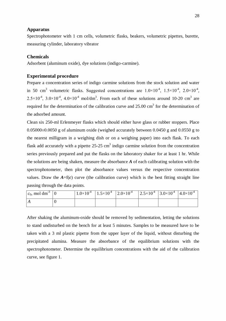
Experimental procedure
Prepare a concentration series of indigo carmine solutions from the stock solution and water
in 50 cm3 volumetric flasks. Suggested concentrations are 1.0×10
-4, 1.5×10
-4, 2.0×10
-4,
2.5×10⁻⁴
, 3.0×10⁻⁴
, 4.0×10⁻⁴
mol/dm3. From each of these solutions around 10-20 cm
3 are
required for the determination of the calibration curve and 25.00 cm3 for the determination of
the adsorbed amount.
Clean six 250-ml Erlenmeyer flasks which should either have glass or rubber stoppers. Place
0.05000±0.0050 g of aluminum oxide (weighed accurately between 0.0450 g and 0.0550 g to
the nearest milligram in a weighing dish or on a weighing paper) into each flask. To each
flask add accurately with a pipette 25-25 cm3 indigo carmine solution from the concentration
series previously prepared and put the flasks on the laboratory shaker for at least 1 hr. While
the solutions are being shaken, measure the absorbance A of each calibrating solution with the
spectrophotometer, then plot the absorbance values versus the respective concentration
values. Draw the A=f(c) curve (the calibration curve) which is the best fitting straight line
passing through the data points.
c0, mol dm-3
0 1.0×10⁻⁴
1.5×10⁻⁴
2.0×10⁻⁴
2.5×10⁻⁴
3.0×10⁻⁴
4.0×10⁻⁴
A 0
After shaking the aluminum-oxide should be removed by sedimentation, letting the solutions
to stand undisturbed on the bench for at least 5 minutes. Samples to be measured have to be
taken with a 3 ml plastic pipette from the upper layer of the liquid, without disturbing the
precipitated alumina. Measure the absorbance of the equilibrium solutions with the
spectrophotometer. Determine the equilibrium concentrations with the aid of the calibration
curve, see figure 1.

29
Figure 1. Determination of the equilibrium concentration of solutions after adsorption with
the aid of the calibration curve (absorption vs. concentration).
Calculation of results
Calculate the adsorbed amounts with the equation (1). Fill in the table below! Plot the
linearized form of Langmuir equation (3). Determine the slope of the line and calculate the am
monolayer capacity. Calculate the specific surface area of the adsorbent (equation 4); the area
occupied by an indigo-carmine molecule on the surface is 1.34 nm2 (recall that 1 nm =10
-9 m).
co (mol/L) 1.0×10⁻⁴
1.5×10⁻⁴
2.0×10⁻⁴
2.5×10⁻⁴
3.0×10⁻⁴
4.0×10⁻⁴
A after adsorption
c (mol dm-3
) after adsorption
m (g): mass of adsorbent
a (mol/g): specific adsorbed
amount
c/a (g dm-3
)
0
0.5
1
0.0E+0 2.0E-4 4.0E-4c0, mol / L
AA(ce)
ce
30
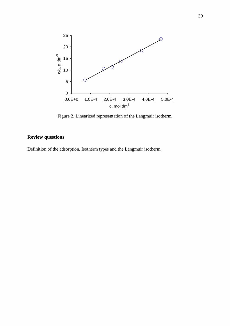
Figure 2. Linearized representation of the Langmuir isotherm.
Review questions
Definition of the adsorption. Isotherm types and the Langmuir isotherm.
0
5
10
15
20
25
0.0E+0 1.0E-4 2.0E-4 3.0E-4 4.0E-4 5.0E-4
c, mol dm3
c/a
, g
dm
-3

31
5. Solubilization
Theory
It is widely observed that soluble amphipathic substances, both ionic and nonionic, show
sharp changes in a variety of colligative physical chemical properties at a well-defined
concentration which is characteristic to the solute in question. These phenomena are attributed
to the association of solute molecules into clusters known as micelles. The concentration at
which micellization occurs is known as the critical micelle concentration, generally
abbreviated CMC. Figure 1 shows the superpositioned curves for a variety of properties (such
as surface tension, electrical, specific and molar conductance, freezing-point depression,
osmotic pressure, turbidity) versus concentration for sodium dodecyl sulfate solutions.
Another interesting property of micelles is their ability to solubilize materials which otherwise
are insoluble in aqueous solutions. Insoluble organic matter, for example, may dissolve in the
interior of the micelle even though it shows minimal solubility in water. Certain oil-soluble
dyes barely color water, but give vividly colored solutions above the cmc. This solubilization
of organic molecules in micelles is known to play an important part in the process of emulsion
polymerization.
Figure 1. Schematic illustration of a variety of properties ( conductivity, osmotic
pressure, turbidity, surface tension, and equivalent conductivity) of sodium dodecyl
sulfate versus concentration.
In discussing micellization, we have intentionally restricted attention to concentration near to
cmc where the micelles are fairly symmetric in shape and they are far enough from each other
~ 0.008 M
~ 0.008 M
Pro
pert
y

32
to be treated as independent entities. At higher concentration, neither of these concentrations
are met and more complex phase equilibria must be considered.
Figure 2. Pictorial represantation of conformation of surfactant molecules (monomers) in a
solution. Above the CMC concentration (a) micelles are formed. At higher surfactant
concentration, the amphiphiles form a variety of structures, here illustrated with (b) a liquid
crystalline lamellar single phase and (c) reversed micelles, an isotropic single phase.
The critical micelle concentration depends on the solvent (generally water), the structure of
surfactant molecules, the salt concentration and the temperature. For charged micelles, the
situation is complicated by the fact that the micelle binds a certain number of counterions
with the remainder required for electroneutrality distributed in an ion atmosphere surrounding
the micelle. The data show that as the salt concentration increases, the cmc decreases, the
degree of aggregation increases, and the effective percent ionization decreases. The cmc of a
nonionic surfactant generally decreases and the size of micelles increases with increasing
temperature because of the decrease of solvation (hydrogen bond) with the temperature. The
solubility of ionic surfactants shows a rapid increase from a certain temperature known as the
Krafft point.
The study of solubilized systems obviously starts with the determination of concentration of
solubilizate which can be incorporated into a given system with the maintenance of a single
isotropic solution. This saturation concentration of solubilizate for a given concentration of
surfactant is termed the maximum additive concentration, which shows the solubilization
ability of the surfactant for the given solubilizate. The maximum additive concentration
increases with increasing surfactant concentration. Above the maximum additive
concentration a second phase of the matter appears. The maximum additive concentration or
the solubilized amount depends on the hydrophilic-hydrophobic character of the organic
matter. The organic molecule, depending on its structure, takes place in the micelle according
to the equalization of polarities (Hardy-Harkins principle).

33
Apparatus
Volumetric flasks, beakers, volumetric pipettes, burette, magnetic stirrer or shaker.
Chemicals
Non-ionic surfactant (e.g. Tween 20 or 40), organic acids (e.g. salicylic acid, benzoic acid or
dodecanoic acid), 0.02 M NaOH solution, absolute alcohol.
Polyoxyethylene sorbitan monolaurate (Tween 20)
(HLB: 16.7)
Experimental procedure
Prepare about 5% stock solution from 2.5 g surfactant in a 50 cm3 volumetric flask. Dilute
from the stock solution 50-50 cm3 surfactant solutions with concentrations of 2%, 1%, 0.5%,
0.2%, 0.1% and 0% (carefully homogenize the solution to prevent foaming). Pour 50 cm3
from each solution into iodine value flasks and add approximately 0.5-0.5 g organic acid into
each of these flasks. It is very important to grind the acid to a fine powder in a mortar before
adding it to the flask. Place the flasks on the magnetic stirrer for 1 hour then separate the
insoluble organic acid from the solution by filtration. Prepare 6 fluted folded filter papers for
the filtration. Pipette 10-10 cm3 aliquots from the equilibrium solutions into Erlenmeyer
flasks then add 5-5 cm3
of propanol and 2-3 drops of phenolphthalein indicator to each flask.
Titrate the solutions with 0.02 M sodium hydroxide until the color of the solutions becomes
pale pink.
34
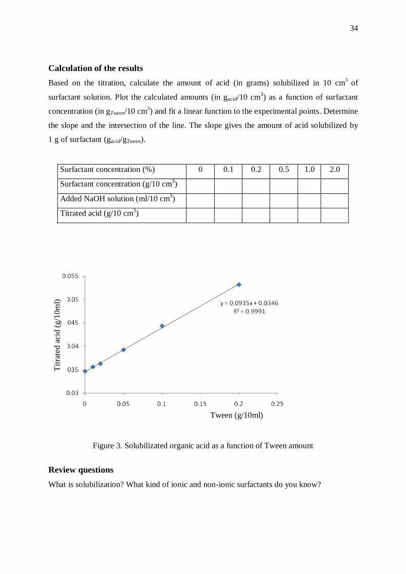
Calculation of the results
Based on the titration, calculate the amount of acid (in grams) solubilized in 10 cm3
of
surfactant solution. Plot the calculated amounts (in gacid/10 cm3) as a function of surfactant
concentration (in gTween/10 cm3) and fit a linear function to the experimental points. Determine
the slope and the intersection of the line. The slope gives the amount of acid solubilized by
1 g of surfactant (gacid/gTween).
Surfactant concentration (%) 0 0.1 0.2 0.5 1.0 2.0
Surfactant concentration (g/10 cm3)
Added NaOH solution (ml/10 cm3)
Titrated acid (g/10 cm3)
Figure 3. Solubilizated organic acid as a function of Tween amount
Review questions
What is solubilization? What kind of ionic and non-ionic surfactants do you know?
Tit
rate
d a
cid (
g/1
0m
l)
Tween (g/10ml)

35
6 Determination of size distribution of a sedimenting suspension
Theory
The size of a spherical homogeneous particle is unequivocally defined by its diameter. When
the particle is irregular additional parameters are needed to correctly define its size. With
some irregular particles so called derived diameters are determined by measuring a size-
dependent property of the particle and relating it to a linear dimension. The most widely used
of these are the equivalent spherical diameters. If an irregular shaped particle is allowed to
settle in a liquid, its terminal velocity may be compared with the terminal velocity of a sphere
of the same density settling under similar conditions. The size of the particle is then equated
to the diameter of the sphere. That is to say we use the diameter of some consubstantial sphere
that has the same sedimentation rate as the particle measured to represent the dimension of the
actual particle. In the laminar flow region, the particle moves with random orientation, the
free-falling diameter becomes the Stokes diameter.
Average diameters. The purpose of the average is to represent a group of individual values in
a simple and concise manner in order to obtain an understanding of the group. It is important,
therefore that the average should be representative of the group. All average diameters are a
measure of central tendency which is unaffected by the relatively few values in the tails of
distribution. The most commonly occurring values are the mode, mean and median. The
mode the value at which the frequency density curve shows a maximum. For the mean:
d
xdx , where is the frequency function. = d for a number distribution; = dW
=x3 d for a volume or weight distribution. The median is the value of 50 % frequency.

36
Figure 1. Cumulative percentage curves for normal distribution.
Figure 1. Relative percentage frequency curves for normal distribution.
The principle of the sedimentation is the determination of the rate at which particles settle out
of a homogeneous suspension. This may be determined by allowing the sediment to fall on to
a balance pan and weighing it. In a sedimentation cylinder h is the height of suspension above
the balance pan in meter; the weight per cent P(t) which has settled out at time t is made up of
two parts; W consists of all particles with a free-falling speed greater than that of rStk as given
by Stokes’ law, where rStk is the size of particle which has a velocity of fall h/t; the other
consist of particles smaller than rStk which have settled because they started off at some
intermediate position (h*<h) in the fluid column.
50
100
0 50 100 150 200
x
%
mean +
mean -
84
16
mean ± ~68 %
15
0
0.005
0.01
0.015
0.02
0.025
0.03
0 20 40 60 80 100 120 140 160 180 200
x
d
/dx
33.5 ; P 1.3
15 ; P 1.065
mean = mode = meadian = 100mean ± =68.26%
mean ± 2=95.5%

37
h
grthv 0
2
9
2/
hence
gt
hrStk
0
2
2
9
h
hence
t
consrStk ;
gh
cons02
9
h
(1)
Where r is radius of particles in meter; and 0 are the densities of the particle and medium;
h is the height of suspension in meter; t is the time of the settling in second; h=0.001 Pas is
the viscosity; g=9.81 m/s2. It can be shown that part of the smaller particles is t dP/dt, so
dtdPtWtP /)( (2)
Since P and t are known, it is possible to determine W using this equation by graphical
differentiation as Figure 2 shows.
Figure 2. Determination of weight percentage oversize, W(r) from a graph of weight of
powder sedimented, P(t) against time, t. Figure 2. Cumulative W(r) and differential dW/dr (r)
distribution functions
Apparatus
Sedimentation cylinder, sedimentation balance
Chemicals
4 g powder, deionized water
Experimental procedure
Measure the distance between the two signs on the sedimentation cylinder (the height of water
column h in meters), then fill the cylinder with distilled water up to mark. Place the cylinder
below the balance and hook up the balance pan to the balance. Start the Sediment program on
the computer then zero the balance with the zero button. Add about 4 g of powder into the
water, stir the suspension and let it about 10 minutes to wet. Stir the suspension thoroughly
moving the balance pan up and down, put the cylinder to its place as fast as you can, set the
.00
.25
.50
.75
1.00
0 5 10 15 20 25
r, micron
W (r)
dW /dr

38
hook of the pan and start the sedimentation. The computer program read the settled weight
(Pt, cg) against time (t). It is necessary to measure until the majority of the powder has settled
out onto the balance pan, this can be assumed to happen when the weight doesn’t change for
about 5-10 minutes. The last value is the maximum weight Pt= or 100%.
Save the data and open it in excel.
h
(m)
P∞
(cg)
medium
(kg m-3
)
solid
(kg m-3
)
h(Pa×s)
1000 2600 0.001
Calculation of the results
t (s) r (m) W (%) t (s) r (m) W (%)
Plot the weight of settled suspension as a function of time, P(t) in %. Determine the weight
percentage oversize, W(t) by graphical differentiation (see figure 1) from the y axial intercepts
of the tangents by 50 s scale units. Calculate the radius from the given times with Stokes’ law
and fill the table above. Plot W(r) = f(r) the cumulative percentage frequency curve (integral
size distribution function). Determine the most commonly occurring value of particle size
from the point inflexion of function of W(r) = f(r), read particle sizes at the 16%; 50% and
84%; see Figure 2. Determine the difference between the size r50% - r84 % and r16 % - r50% .
Dicuss the results

39
Review questions
What is the Stokes’ radius? What is the advantage and disadvantage of this method?
Characterize the normal distribution.

40
7. Characterization of substances of different rheological properties by
Brookfield DV-II+ rotational viscosimeter
The theoretical background of rheology can be found in the description of Exercise 1
(Rheological characterization of concentrated emulsions) and in the Appendix. Please read the
mentioned sections to prepare yourself for the short test.
Principles of the measurement:
The rheological properties of substances are studied in viscosimetry by rotating spindles. The
studied substance exerts rolling friction toward the rotation of the spindle (cylinder), by this
way reducing the rate of rotation. The rolling friction can be characterized by the strength of
the friction or by the shear stress (), that is a portion of strength of friction referred to the unit
of area of the spindle. The cylinder can be rotated at different angular velocity and the related
shear stress values can be determined. The spindle is connected to the rotatory shaft through a
spiral spring driven by a synchronous motor. The rotation of the rotatory shaft is transferred to
the spindle through the spiral spring. In the presence of viscous media the spring is streched
(wounded) due to the inertia of the spindle.
The viscometer measures the torque necessary to overcome the viscous resistance to the
induced movement. The degree to which the spring is wound or deflected is proportional to
the viscosity of the fluid. The spring deflection is measured with a rotary transducer. The
revolutions per minute (RPM) of the rotatory shaft can be adjusted between 0 and 100 RPM
through gears. The velocity gradient is proportional to the angular velocity of the motor.
Execution of the measurements
Switch on the rheometer with the switch at the back. Remove any spindle if mounted, then
press any key. After the automatic zero, choose the appropriate spindle and mount it to the
end of the shaft. For this procedure ask for the help of the instructors.
Mounting the spindle: fix the shaft with
one hand, screw on the spindle (it is left-hand thread!), check the fixing.

41
Write the number of the spindle in your report sheet. When installing the spindle first
immerse it to the sample, avoiding to hit it to the walls of the container. The beaker should be
positioned so that the spindle is in the middle, and the spindle should be immersed below the
surface of the sample by the mark on it. After this press any key on the instrument again.
When choosing the proper spindle for a measurement, the goal is that the viscosimeter torque,
α displayed in % should be between 10 and 100. When the torque is greater then 100, EEEE
overflow signal is displayed.
To start the measurements, chose the proper speed with the up and down arrows using table 1.
When the speed is chosen, push set speed button until the RPM is flashing on the screen to
apply the speed. After the measurement of the samples is started, always wait for the
stabilization of α before reading the signal, then set the next speed. Ask for the help of the
instructors to change the spindles for the next sample.
Necessary equations for the calculations:
Viscosity h (mPas)= 100×TK×SMC×SRC× /D (1)
Shear rate D (s-1
) = RPM×SRC (2)
Shear stress m2 = TK×SMC×SRC×3
Where is the torque given in %, RPM is the revolutions per minute, TK is spring strength (for spindles of RV type it has the value of 1), SMC gives the viscosity equal to 1 unit of scale, SRC (Spindle Rate Constant) is a
constant characteristic related to the geometry of the spindle (for cylindrical spindles it can be calculated or it is
given in charts, otherwise take it to be 1)
spindle data :
LV type* TK=0.09373 *in 600 ml beaker
Code 4 3 2 1
SMC 60 12 2.4 0.48 1 unit of scale in mPas
SF*N=100*SMC 6000 1200 240 48 The whole scale in mPas
RV type * TK=1
RV1 RV2 RV3 RV4 RV5 RV6 RV7
Code 1 2 3 4 5 6 7
SMC 1 4 10 20 40 100 400
SF*N=100*SMC 100 400 1000 2000 4000 10000 40000
TK=1 T-A T-B T-C T-D T-E T-F
Code 91 92 93 94 95 96
SMC 20 40 100 200 500 1000
SF*N=100*SMC 2000 4000 10000 20000 50000 100000
TK=1 SC4-28 ULA
Code 28 00
SMC 50 0.64
SF*N=100*SMC 5000 64 1 cP=1mPas
SRC 0.28 1.223 16.0 ml (with cap)

42
Samples to be measured:
1. Rheological study of 10% wallpaper paste (Na carboxymethylcellulose)
Before the start of the measurement, homogenize the sample by rotating the chosen spindle at
100 RPM for 5 minutues, after that wait for 10 minutes at 0 RPM to let the sample regain its
unstrained structure. Thereafter, determine the torque values of the wallpaper paste at
increasing and decreasing RPM values following the instructions given earlier. For data
recording and evaluation, use table 1.
2. Rheological study of honey sample
Repeat the previous measurement with the honey sample using the appropriate spindle. For
data recording and evaluation, use table 1.
3. Rheological study of 2,5% PVA (polyvinyl alcohol)–borax mixture
Repeat the previous measurement with the PVA–borax mixture using the appropriate spindle.
For the homogenization of the sample use 60 RPM instead of 100 RPM. For data recording
and evaluation, use table 1.
Table 1 Sample: Spindle: SMC:
RPM (1/min) α (%) D (1/s) τ (Pa) η (mPas)
0.3
0.5
0.6
1
1.5
2
2.5
3
4
5
6
10
12
20
30

43
50
60
100
60
50
30
20
12
10
6
5
4
3
2.5
2
1.5
1
0.6
0.5
0.3
After all of the measurements have been performed, plot the viscosity curves h=f() and flow
curves D =f() of the samples. The data points measured at increasing and decreasing RPM
values should be plotted in the same graph (Thus you have to submit 6 graphs altogether).
Determine the rheological class of the samples using figure 1 in Exercise 1. Decide if there is
any hysteresis or not in the curves and give an explanation for these observations (see
Exercise 1).
Interpret the results.

44
8. Steric and electrostatic stabilization mechanisms of colloidal dispersions
Theory
DVLO theory suggests that the stability of a colloidal system is determined by the sum of the
van der Waals attractive (VA) and electrical double layer repulsive (VR) forces that exist
between particles as they approach each other due to the Brownian motion. This theory
proposes that an energy barrier resulting from the repulsive force prevents two particles to
approach one another and to adhere. But if the
particles collide with sufficient energy to
overcome that barrier, aggregation may start.
DVLO theory assumes that the stability of a
particle in solution is dependent upon its total
potential energy function VT.
Lyophobic colloids can be stabilized kinetically by electrostatic or steric ways. In case of
electrostatic stabilization, the repulsion of surface charges of sol particles hinder the frequent
collision of particles, by this way the extent of sol aggregation is reduced. The surface charge
depends on the property and quantity of positive and negative ions present in the solution,
since the adsorbtion of different kind of ions to the surface of sol particles is variant. If the
composition of the solution is such that the surface charge of colloid is zero (point of zero
charge), the electrostatic repulsion ceases to exist and the coagulation of the sol is accelerated.
Any increase in surface charge in whichevere direction hinders the aggregation.
In case of steric stabilization the material adsorbed to the surface of the colloid particles
(usually some kind of macromolecule or surfactant) hinders the direct contact of sol particles
and by this way the aggregation, as well. If the macromolecule is adsorbed to the surface only
in small concentration (thus one macromolecule is in connection with more than one sol
particle), in contrast with the previously mentioned protecting effecet, the sol particles will be
sensitized to coagulation due to the so-called bridging flocculation mechanism.

45
0 ln ln PZC
kTa a
ze
Electrostatic (a) and steric stabilization (b) mechanisms of colloidal dispersions, and bridging
flocculation (c).
The charge which is carried by surface determines its electrostatic potential. For this reason
they are called the potential-determining ions. We can calculate the surface potential on the
crystals of silver halids by considering the equilibrium between the surface of charged crystal
and the ions in the surrounding solution:
For the ions involved:
)log(log60 ,0 pzcAgAg aa and
)log(log60 ,0 pzcClCl aa
where Ψ0 is the surface potential, a is the activity of the potential-determining ion (for dilute
solutions a ≈ c), aion,pzc is the ion activity at the point of zero charge.
log aAg,pzc= -4.5 ([Agpzc]≈2.9×10⁻⁵
M) and log aCl,pzc= -5.2 ([Clpzc] =6.3×10⁻⁶
M) and the
solubility product for AgCl is Ksp=1.8×10⁻¹⁰
mol2 dm
-6.
Chemicals
0.05% PVA solution, 0.01 M AgNO3 and 0.01 M KCl solution, deionized water.
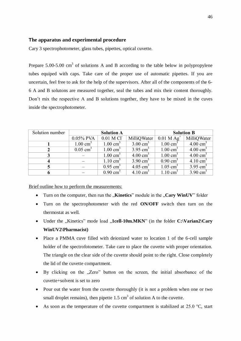
46
The apparatus and experimental procedure
Cary 3 spectrophotometer, glass tubes, pipettes, optical cuvette.
Prepare 5.00-5.00 cm3 of solutions A and B according to the table below in polypropylene
tubes equiped with caps. Take care of the proper use of automatic pipettes. If you are
uncertain, feel free to ask for the help of the supervisors. After all of the components of the 6-
6 A and B solutons are measured together, seal the tubes and mix their content thoroughly.
Don’t mix the respective A and B solutions together, they have to be mixed in the cuves
inside the spectrophotometer.
Solution number Solution A Solution B
0.05% PVA 0.01 M Cl-
MilliQWater 0.01 M Ag+
MilliQWater
1 1.00 cm3 1.00 cm
3 3.00 cm
3 1.00 cm
3 4.00 cm
3
2 0.05 cm3 1.00 cm
3 3.95 cm
3 1.00 cm
3 4.00 cm
3
3 – 1.00 cm3 4.00 cm
3 1.00 cm
3 4.00 cm
3
4 – 1.10 cm3 3.90 cm
3 0.90 cm
3 4.10 cm
3
5 – 0.95 cm3 4.05 cm
3 1.05 cm
3 3.95 cm
3
6 – 0.90 cm3 4.10 cm
3 1.10 cm
3 3.90 cm
3
Brief outline how to perform the measurements:
Turn on the computer, then run the „Kinetics” module in the „Cary WinUV” folder
Turn on the spectrophotometer with the red ON/OFF switch then turn on the
thermostat as well.
Under the „Kinetics” mode load „1cell-10m.MKN” (in the folder C:\Varian2\Cary
WinUV2\Pharmacist)
Place a PMMA cuve filled with deionized water to location 1 of the 6-cell sample
holder of the spectrofotometer. Take care to place the cuvette with proper orientation.
The triangle on the clear side of the cuvette should point to the right. Close completely
the lid of the cuvette compartment.
By clicking on the „Zero” button on the screen, the initial absorbance of the
cuvette+solvent is set to zero
Pour out the water from the cuvette thoroughly (it is not a problem when one or two
small droplet remains), then pipette 1.5 cm3 of solution A to the cuvette.
As soon as the temperature of the cuvette compartment is stabilized at 25.0 °C, start
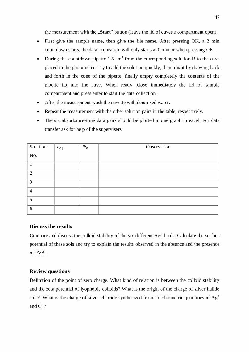
47
the measurement with the „Start” button (leave the lid of cuvette compartment open).
First give the sample name, then give the file name. After pressing OK, a 2 min
countdown starts, the data acquisition will only starts at 0 min or when pressing OK.
During the countdown pipette 1.5 cm3 from the corresponding solution B to the cuve
placed in the photometer. Try to add the solution quickly, then mix it by drawing back
and forth in the cone of the pipette, finally empty completely the contents of the
pipette tip into the cuve. When ready, close immediately the lid of sample
compartment and press enter to start the data collection.
After the measurement wash the cuvette with deionized water.
Repeat the measurement with the other solution pairs in the table, respectively.
The six absorbance-time data pairs should be plotted in one graph in excel. For data
transfer ask for help of the supervisers
Solution
No.
cAg Ψ0 Observation
1
2
3
4
5
6
Discuss the results
Compare and discuss the colloid stability of the six different AgCl sols. Calculate the surface
potential of these sols and try to explain the results observed in the absence and the presence
of PVA.
Review questions
Definition of the point of zero charge. What kind of relation is between the colloid stability
and the zeta potential of lyophobic colloids? What is the origin of the charge of silver halide
sols? What is the charge of silver chloride synthesized from stoichiometric quantities of Ag+
and Cl-?
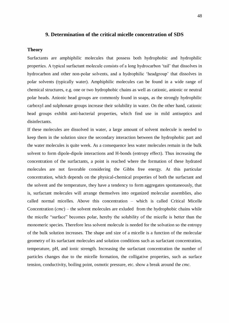
48
9. Determination of the critical micelle concentration of SDS
Theory
Surfactants are amphiphilic molecules that possess both hydrophobic and hydrophilic
properties. A typical surfactant molecule consists of a long hydrocarbon ‘tail’ that dissolves in
hydrocarbon and other non-polar solvents, and a hydrophilic ‘headgroup’ that dissolves in
polar solvents (typically water). Amphiphilic molecules can be found in a wide range of
chemical structures, e.g. one or two hydrophobic chains as well as cationic, anionic or neutral
polar heads. Anionic head groups are commonly found in soaps, as the strongly hydrophilic
carboxyl and sulphonate groups increase their solubility in water. On the other hand, cationic
head groups exhibit anti-bacterial properties, which find use in mild antiseptics and
disinfectants.
If these molecules are dissolved in water, a large amount of solvent molecule is needed to
keep them in the solution since the secondary interaction between the hydrophobic part and
the water molecules is quite week. As a consequence less water molecules remain in the bulk
solvent to form dipole-dipole interactions and H-bonds (entropy effect). Thus increasing the
concentration of the surfactants, a point is reached where the formation of these hydrated
molecules are not favorable considering the Gibbs free energy. At this particular
concentration, which depends on the physical-chemical properties of both the surfactant and
the solvent and the temperature, they have a tendency to form aggregates spontaneously, that
is, surfactant molecules will arrange themselves into organized molecular assemblies, also
called normal micelles. Above this concentration – which is called Critical Micelle
Concentration (cmc) – the solvent molecules are exluded from the hydrophobic chains while
the micelle “surface” becomes polar, hereby the solubility of the micelle is better than the
monomeric species. Therefore less solvent molecule is needed for the solvation so the entropy
of the bulk solution increases. The shape and size of a micelle is a function of the molecular
geometry of its surfactant molecules and solution conditions such as surfactant concentration,
temperature, pH, and ionic strength. Increasing the surfactant concentration the number of
particles changes due to the micelle formation, the colligative properties, such as surface
tension, conductivity, boiling point, osmotic pressure, etc. show a break around the cmc.
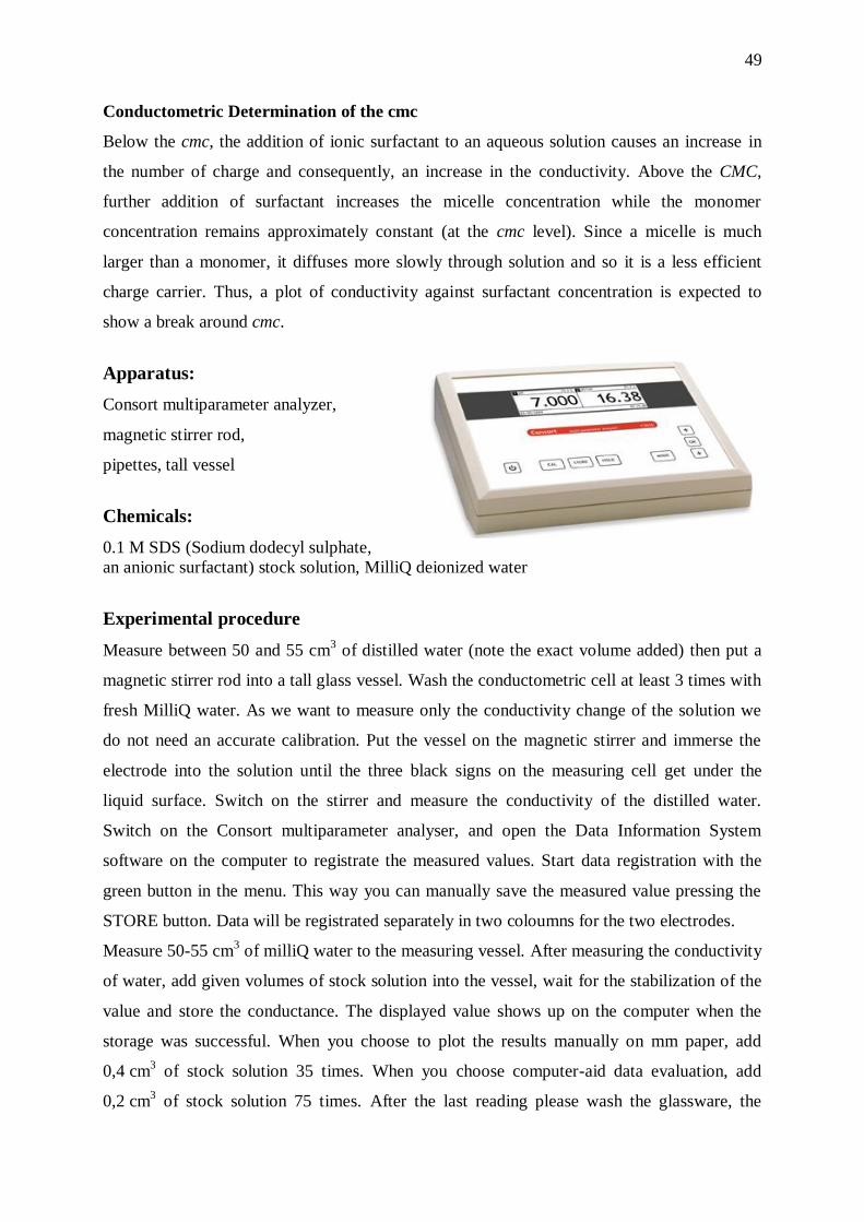
49
Conductometric Determination of the cmc
Below the cmc, the addition of ionic surfactant to an aqueous solution causes an increase in
the number of charge and consequently, an increase in the conductivity. Above the CMC,
further addition of surfactant increases the micelle concentration while the monomer
concentration remains approximately constant (at the cmc level). Since a micelle is much
larger than a monomer, it diffuses more slowly through solution and so it is a less efficient
charge carrier. Thus, a plot of conductivity against surfactant concentration is expected to
show a break around cmc.
Apparatus:
Consort multiparameter analyzer,
magnetic stirrer rod,
pipettes, tall vessel
Chemicals:
0.1 M SDS (Sodium dodecyl sulphate,
an anionic surfactant) stock solution, MilliQ deionized water
Experimental procedure
Measure between 50 and 55 cm3 of distilled water (note the exact volume added) then put a
magnetic stirrer rod into a tall glass vessel. Wash the conductometric cell at least 3 times with
fresh MilliQ water. As we want to measure only the conductivity change of the solution we
do not need an accurate calibration. Put the vessel on the magnetic stirrer and immerse the
electrode into the solution until the three black signs on the measuring cell get under the
liquid surface. Switch on the stirrer and measure the conductivity of the distilled water.
Switch on the Consort multiparameter analyser, and open the Data Information System
software on the computer to registrate the measured values. Start data registration with the
green button in the menu. This way you can manually save the measured value pressing the
STORE button. Data will be registrated separately in two coloumns for the two electrodes.
Measure 50-55 cm3 of milliQ water to the measuring vessel. After measuring the conductivity
of water, add given volumes of stock solution into the vessel, wait for the stabilization of the
value and store the conductance. The displayed value shows up on the computer when the
storage was successful. When you choose to plot the results manually on mm paper, add
0,4 cm3 of stock solution 35 times. When you choose computer-aid data evaluation, add
0,2 cm3 of stock solution 75 times. After the last reading please wash the glassware, the
50
sirring rod and the measuring cell accurately with distilled water and leave the electrode
immersed in water. Fill the conductance values in the Table.
Calculation:
Calculate the derived conductivity (’), the molar conducitivity () using the following
equations:
watermeasured '
c
' (Calculate Λ in SI units!)
Plot the c-and ³√c - (Lottermoser-diagram) curves, find the breakpoints on the curves and
calculate the CMC values from the two figures.
Determine the CMC value of SDS, and discuss it. (literature data: 0.008 mol dm-3
at 25oC)
Review questions
What kind of ionic and non-ionic surfactants do you know? Define the critical micelle
concentration! Describe the reasons of micelle formation!
0.0E+00
5.0E-02
1.0E-01
1.5E-01
2.0E-01
0 5 10 15 20 25c(mol m-3)
(S
m-1
)
8.0E-03
1.0E-02
1.2E-02
1.4E-02
0.05 0.10 0.15 0.20 0.25 0.30
(S
m2m
ol
-1)
3√c

n Vincrements
(cm3)
Vtotal added
(cm3)
Vtotal
(cm3)
c
(mol dm-3
)
c
(mol m-3
)
measured
(S cm-1
)
(S cm-1
)
(S m
-1)
³√c
(mol1/3
m-1
)
(S m2
mol-1)
0. 0 0 50 or 55 0 0
1.
2.
3.
4.
5.
6.
7.
8.
9.
10.
…
Appendix
1. Basic concepts of rheology
Isaac Newton defined viscosity by considering the following model: two parallel planes of fluid of
equal area “A” are separated by a distance “dy” and are moving in the same direction (x) at different
velocities “v1” and “v2”. Newton assumed that the force required maintaining this difference in speed
was proportional to the velocity gradient.
To express this, Newton wrote: dy
dv
A
Fh where h is a constant for a given material and is called its
“viscosity”.
Rheological classification of materials
Fluids are normally divided into three different groups according to their flow behaviour:
Newtonian fluids
The viscosity of a Newtonian fluid is dependent only on temperature but not on shear rate and time.
Examples: water, milk, sugar solution, mineral oil.
Non-Newtonian fluids, time independent
The viscosity of a Non-Newtonian time independent fluid is dependent not only on temperature but
also on shear rate.
Depending on how viscosity changes with shear rate the flow behaviour is characterized as:
shear thinning or pseudoplastic - the viscosity decreases with increased shear rate
shear thickening or dilatant - the viscosity increases with increased shear rate
plastic - exhibits a so-called yield value, i.e. a certain shear stress must be applied before flow occurs
Examples of shear thinning fluids: paint, shampoo, slurries, fruit juice concentrates, ketchup,
Examples of shear thickening fluids: wet sand, concentrated starch suspensions
Examples of plastic fluids: tomato paste, tooth paste, hand cream, some ketchups, grease
Non-Newtonian fluids, time dependent
The viscosity of the fluid is dependent on temperature, shear rate and time.
Depending on how viscosity changes with time the flow behaviour is characterized as:
thixotropic (time thinning, i.e. viscosity decreases with time) Examples: yoghurt, paint
rheopectic (time thickening, i.e. viscosity increases with time) Examples gypsum paste

53
Thixotropic fluids are quite common in chemicals as well as in food industry. Rheopectic fluids are
very rare.
Figure 1. Flow and viscosity curves of newtonian and non-newtonian time-independent fluids.
1. ideal (newtonian), 2. shear thinning or pseudoplastic, 3. shear thickening or dilatant, 4. ideal plastic
(Bingham type), 5. plastic (pseudo-plastic type), 6. plastic (dilatant type)
Newtonian fluids. The type of flow behaviour Newton assumed for all fluids is called, not
surprisingly, “Newtonian”. It is, however, only one of several types of flow behaviour you may
encounter. A Newtonian fluid is represented graphically in Figure 1, curve 1, which shows that the
relationship between shear stress and shear rate is a straight line. In the other graph, curve 2 shows that
the fluid’s viscosity remains constant as the shear rate is varied. What this means in practice is that at a
given temperature the viscosity of a Newtonian fluid will remain constant regardless of which
Viscometer model, spindle or speed you use to measure it. Newtonians are obviously the easiest fluids
to measure – just grab your viscometer and go it. They are not, unfortunately, as common as that much
more complex group of fluids, the non-Newtonians, which will be discussed in the next.
Non-Newtonian fluids. A non-Newtonian fluid is broadly defined as for which the relationship / D
is not constant. In other words, when the shear rate is varied, the shear stress doesn’t vary in the same
proportion (or even necessarily in the same direction). The viscosity of such fluids will therefore tend
to change as the shear rate is varied. Thus, the experimental parameters of a Viscometer model, spindle
and speed all have an effect on the measured viscosity called apparent viscosity of fluid, which is
accurate only when explicit experimental parameters are furnished and adhered to.
Non-Newtonian flow is probably a mechanical proposition. As non-symmetrical objects pass by each
other, as happens during flow, their size, shape, and cohesiveness will determine how much force is
required to move them. At another rate of shear, the alignment of the objects may be different and
more or less force may be required to maintain motion. By non-symmetrical objects, we refer to large
molecules, colloidal particles, and other suspended materials such as clays, fibre, and crystals.
(Pa)0
D(s
-1)
(Pa)0
D(s
-1)
(Pa)0
D(s
-1)
1
2
3
4
5
6
(Pa)0
h(P
as)
1
2
3
4
5
6

54
There are several types of Non-Newtonian flow behaviour, characterized by the way a fluid’s viscosity
changes in response to variations in shear rate. The most common types of Non-Newtonian fluids you
may encounter include:
Pseudoplastic. This type of fluid will display a decreasing viscosity with an increasing shear rate, as
shown in Figure 1, curve 2 . Probably the most common of non-Newtonian fluids, pseudoplastics
include paints, emulsions, and dispersions of many types. This type of flow behaviour is sometimes
called “shear-thinning”.
Dilatant. Increasing viscosity with an increasing shear rate characterizes the dilatant fluid. Although
rarer than pseudoplasticity, dilatancy is frequently observed in fluids containing high levels of
deflocculated solids, such as clay slurries, corn starch in water, and sand/water mixtures. Dilatancy is
also referred to as “shear-thickening” flow behavior (in Figure 1, curve 3). Plastic. This type of fluid
will behave as solid under static conditions. A certain amount of force must be applied to the fluid
before any flow is induced; this force is called “yield value”. Tomato ketchup is a good example of
this type of fluid; its value will often make it refuse to pour from the bottle until the bottle is shaken or
struck, allowing the ketchup to gush freely. Once the yield value is exceeded and flow begins, plastic
fluids may display Newtonian, pseudoplastic, or dilatant flow characteristics. See Figure 1, curve 4-6.
So far we have only discussed the effect of shear rate on non-Newtonian fluids.
Emulsions and creams
One of the major characteristics to study is the state of aggregation of the sample material. Many
pharmaceutical and cosmetic processes such as new ingredient selections, formulation preparations,
material packaging, and shelf storage are associated with a complex flow behavior of these materials.
The application and acceptance of pharmaceuticals and cosmetics are also dependent on the flow
properties of the final product. Therefore, rheological measurements, an important route to reveal the
flow and deformation behaviors of materials, cannot only improve efficiency in processing but can
also help formulators and end users find pharmaceutical and cosmetic products that are optimal for
their individual needs. In general, rheological measurements on pharmaceutical and cosmetic materials
are performed for the following reasons: 1) to understand the fundamental nature of a system; 2) for
quality control of raw materials, final products, and manufacturing processes such as mixing, pumping,
packaging, and filling; and 3) to study the effect of different parameters such as formulation, storage
time, and temperature on the quality and acceptance of a final product. Pharmaceutical and cosmetic
materials range in consistency from fluid to solid. Semisolid products are the most difficult materials
to characterize rheologically because they combine both liquid and solid properties within the same
material. The majority of pharmaceutical materials are ointments, creams, pastes, and gels—all

55
semisolids. To understand these complex flows, commercial medical creams, shampoos, and e.g.
children’s cough syrup are generally tested by rheometry.