chemical physics of colloid systems and interfaces · pdf file7 chemical physics of colloid...

7 Chemical Physics of Colloid Systemsand Interfaces

Peter A. Kralchevsky, Krassimir D. Danov, and Nikolai D. Denkov

CONTENTS

7.1 Introduction ................................................................................................................................................................... 1997.2 Surface Tension of Surfactant Solutions....................................................................................................................... 200

7.2.1 Static Surface Tension ....................................................................................................................................... 2007.2.1.1 Nonionic Surfactants ........................................................................................................................... 2007.2.1.2 Ionic Surfactants .................................................................................................................................. 206

7.2.2 Dynamic Surface Tension ................................................................................................................................. 2137.2.2.1 Adsorption under Diffusion Control ................................................................................................... 2137.2.2.2 Small Initial Perturbation..................................................................................................................... 2147.2.2.3 Large Initial Perturbation..................................................................................................................... 2157.2.2.4 Generalization for Ionic Surfactants.................................................................................................... 2177.2.2.5 Adsorption under Barrier Control ....................................................................................................... 2187.2.2.6 Dynamics of Adsorption from Micellar Surfactant Solutions ............................................................ 220

7.3 Capillary Hydrostatics and Thermodynamics ............................................................................................................... 2257.3.1 Shapes of Fluid Interfaces ................................................................................................................................. 225

7.3.1.1 Laplace and Young Equations ............................................................................................................ 2257.3.1.2 Solutions of Laplace Equations for Menisci of Different Geometry .................................................. 2277.3.1.3 Gibbs–Thomson Equation ................................................................................................................... 2307.3.1.4 Kinetics of Ostwald Ripening in Emulsions ....................................................................................... 231

7.3.2 Thin Liquid Films and PBs ............................................................................................................................... 2337.3.2.1 Membrane and Detailed Models of a Thin Liquid Film..................................................................... 2337.3.2.2 Thermodynamics of Thin Liquid Films .............................................................................................. 2347.3.2.3 Transition Zone between Thin Film and PB....................................................................................... 2367.3.2.4 Methods for Measuring Thin Film Contact Angles ............................................................................ 239

7.3.3 Lateral Capillary Forces between Particles Attached to Interfaces ................................................................... 2397.3.3.1 Particle–Particle Interactions ............................................................................................................... 2397.3.3.2 Particle–Wall Interactions.................................................................................................................... 2437.3.3.3 Electrically Charged Particles at Liquid Interfaces ............................................................................. 244

7.4 Surface Forces ............................................................................................................................................................... 2487.4.1 Derjaguin Approximation .................................................................................................................................. 2487.4.2 van der Waals Surface Forces ........................................................................................................................... 2497.4.3 Electrostatic Surface Forces............................................................................................................................... 251

7.4.3.1 Two Identically Charged Planes.......................................................................................................... 2517.4.3.2 Two Nonidentically Charged Planes................................................................................................... 2537.4.3.3 Two Charged Spheres ......................................................................................................................... 254

7.4.4 Derjaguin–Landau–Verwey–Overbeek (DLVO) Theory .................................................................................. 2557.4.5 Non-DLVO Surface Forces ............................................................................................................................... 255

7.4.5.1 Ion Correlation Forces......................................................................................................................... 2557.4.5.2 Steric Interaction.................................................................................................................................. 2567.4.5.3 Oscillatory Structural Forces ............................................................................................................... 2597.4.5.4 Repulsive Hydration and Attractive Hydrophobic Forces .................................................................. 2637.4.5.5 Fluctuation Wave Forces..................................................................................................................... 267

197

Birdi/Handbook of Surface and Colloid Chemistry 7327_C007 Final Proof page 197 14.10.2008 10:28am Compositor Name: DeShanthi

© 2009 by Taylor & Francis Group, LLC

7.5 Hydrodynamic Interactions in Dispersions ................................................................................................................... 2687.5.1 Basic Equations and Lubrication Approximation ............................................................................................. 2687.5.2 Interaction between Particles of Tangentially Immobile Surfaces .................................................................... 271

7.5.2.1 Taylor and Reynolds Equations, and Influence of the Particle Shape................................................ 2717.5.2.2 Interactions among Nondeformable Particles at Large Distances....................................................... 2727.5.2.3 Stages of Thinning of a Liquid Film................................................................................................... 2757.5.2.4 Dependence of Emulsion Stability on the Droplet Size ..................................................................... 278

7.5.3 Effect of Surface Mobility ................................................................................................................................. 2807.5.3.1 Diffusive and Convective Fluxes at an Interface—Marangoni Effect................................................ 2817.5.3.2 Fluid Particles and Films of Tangentially Mobile Surfaces................................................................ 2827.5.3.3 Bancroft Rule for Emulsions............................................................................................................... 2857.5.3.4 Demulsification.................................................................................................................................... 287

7.5.4 Interactions in Nonpreequilibrated Emulsions .................................................................................................. 2887.5.4.1 Surfactant Transfer from Continuous to Disperse Phase (Cyclic Dimpling)...................................... 2887.5.4.2 Surfactant Transfer from Disperse to Continuous Phase (Osmotic Swelling).................................... 2897.5.4.3 Equilibration of Two Droplets across a Thin Film ............................................................................. 290

7.5.5 Hydrodynamic Interaction of a Particle with an Interface ................................................................................ 2917.5.5.1 Particle of Immobile Surface Interacting with a Solid Wall ............................................................... 2917.5.5.2 Fluid Particles of Mobile Surfaces ...................................................................................................... 293

7.5.6 Bulk Rheology of Dispersions .......................................................................................................................... 2957.6 Kinetics of Coagulation................................................................................................................................................. 299

7.6.1 Irreversible Coagulation..................................................................................................................................... 2997.6.2 Reversible Coagulation...................................................................................................................................... 3027.6.3 Kinetics of Simultaneous Flocculation and Coalescence in Emulsions............................................................ 303

7.7 Mechanisms of Antifoaming ......................................................................................................................................... 3057.7.1 Location of Antifoam Action—Fast and Slow Antifoams................................................................................ 3067.7.2 Bridging–Stretching Mechanism ....................................................................................................................... 3077.7.3 Role of the Entry Barrier ................................................................................................................................... 308

7.7.3.1 Film Trapping Technique (FTT) ......................................................................................................... 3097.7.3.2 Critical Entry Pressure for Foam Film Rupture .................................................................................. 3097.7.3.3 Optimal Hydrophobicity of Solid Particles ......................................................................................... 3107.7.3.4 Role of the Prespread Oil Layer.......................................................................................................... 311

7.7.4 Mechanisms of Compound Exhaustion and Reactivation................................................................................. 3127.8 Electrokinetic Phenomena in Colloids .......................................................................................................................... 314

7.8.1 Potential Distribution at a Planar Interface and around a Sphere ..................................................................... 3157.8.2 Electroosmosis ................................................................................................................................................... 3177.8.3 Streaming Potential............................................................................................................................................ 3197.8.4 Electrophoresis................................................................................................................................................... 3197.8.5 Sedimentation Potential ..................................................................................................................................... 3227.8.6 Electrokinetic Phenomena and Onzager Reciprocal Relations ......................................................................... 3237.8.7 Electric Conductivity and Dielectric Response of Dispersions......................................................................... 324

7.8.7.1 Electric Conductivity ........................................................................................................................... 3247.8.7.2 Dispersions in Alternating Electrical Field ......................................................................................... 325

7.8.8 Anomalous Surface Conductance and Data Interpretation ............................................................................... 3287.8.9 Electrokinetic Properties of Air–Water and Oil–Water Interfaces .................................................................... 329

7.9 Optical Properties of Dispersions and Micellar Solutions ............................................................................................ 3307.9.1 Static Light Scattering ....................................................................................................................................... 330

7.9.1.1 Rayleigh Scattering.............................................................................................................................. 3307.9.1.2 Rayleigh–Debye–Gans (RDG) Theory ............................................................................................... 3327.9.1.3 Theory of Mie...................................................................................................................................... 3357.9.1.4 Interacting Particles ............................................................................................................................. 3357.9.1.5 Depolarization of Scattered Light ....................................................................................................... 3387.9.1.6 Polydisperse Samples .......................................................................................................................... 3397.9.1.7 Turbidimetry ........................................................................................................................................ 339

7.9.2 DLS.................................................................................................................................................................... 3407.9.2.1 DLS by Monodisperse, Noninteracting Spherical Particles ................................................................ 3407.9.2.2 DLS by Polydisperse, Noninteracting Spherical Particles .................................................................. 342


198 Handbook of Surface and Colloid Chemistry


7.9.2.3 DLS by Nonspherical Particles ........................................................................................................... 3447.9.2.4 Effect of the Particle Interactions ........................................................................................................ 3457.9.2.5 Concentrated Dispersions: Photon Cross-Correlation Techniques, Fiber Optics DLS,

and Diffusing Wave Spectroscopy (DWS) ......................................................................................... 3497.9.3 Application of Light Scattering Methods to Colloidal Systems ....................................................................... 350

7.9.3.1 Surfactant Solutions............................................................................................................................. 3507.9.3.2 Dispersions .......................................................................................................................................... 352

7.9.4 Recent Developments in Light Scattering Techniques ..................................................................................... 3537.9.4.1 Opaque Systems .................................................................................................................................. 3537.9.4.2 Small Angle Light Scattering .............................................................................................................. 3537.9.4.3 Multispeckle DLS................................................................................................................................ 354

Acknowledgment ..................................................................................................................................................................... 354References ................................................................................................................................................................................ 355

7.1 INTRODUCTION

A colloidal system represents a multiphase (heterogeneous) system, in which at least one of the phases exists in the form of verysmall particles: typically smaller than 1 mm but still much larger than the molecules. Such particles are related to phenomenalike Brownian motion, diffusion, and osmosis. The terms microheterogeneous system and disperse system (dispersion) aremore general because they include also bicontinuous systems (in which none of the phases is split into separate particles) andsystems containing larger, non-Brownian, particles. The term dispersion is often used as a synonym of colloidal system.

Classification of the colloids with respect to the state of aggregation of the disperse and the continuous phases is shown inTable 7.1. Some examples are following.

1. Examples for gas-in-liquid dispersions are the foams or the boiling liquids. Gas-in-solid dispersions are the variousporous media like filtration membranes, sorbents, catalysts and isolation materials.

2. Examples for liquid-in-gas dispersions are the mist, the clouds, and other aerosols. Liquid-in-liquid dispersions are theemulsions. At room temperature there are only four types of mutually immiscible liquids: water, hydrocarbon oils,fluorocarbon oils, and liquid metals (Hg and Ga). Many raw materials and products in food and petroleum industriesexist in the form of oil-in-water (O=W) or water-in-oil (W=O) emulsions. The soil and some biological tissues can beconsidered as liquid-in-solid dispersions.

3. Smoke, dust, and some other aerosols are examples for solid-in-gas dispersions. The solid-in-liquid dispersions aretermed as suspensions or sols. The pastes and some glues are highly concentrated suspensions. The gels representbicontinuous structures of solid and liquid. Solid-in-solid dispersions are some metal alloys, many kinds of rocks,some colored glasses, etc.

Below we will consider mostly liquid dispersions, i.e., dispersions with liquid continuous phase like foams, emulsions, andsuspensions. Sometimes these are called complex fluids.

In general, the area of the interface between the disperse and continuous phases is rather large. For instance, 1 cm3 ofdispersion with particles of radius 100 nm and volume fraction 30% contains interface of area about 10 m2. This is the reasonwhy the interfacial properties are of crucial importance for the properties and stability of colloids.

The stabilizing factors for dispersions are the repulsive surface forces, the particle thermal motion, the hydrodynamicresistance of the medium, and the high surface elasticity of fluid particles and films.

TABLE 7.1Types of Disperse Systems

Continuous Phase

Disperse Phase Gas Liquid Solid

Gas — Gas in liquid Gas in solidLiquid Liquid in gas L1 in L2 Liquid in solidSolid Solid in gas Solid in liquid S1 in S2


Chemical Physics of Colloid Systems and Interfaces 199


On the contrary, the factors destabilizing dispersions are the attractive surface forces, the factors suppressing the repulsivesurface forces, and the low surface elasticity, gravity and other external forces tending to separate the phases.

Sections 7.2 and 7.3 consider effects related to the surface tension of surfactant solution and capillarity. Section 7.4 presentsa review on the surface forces due to the intermolecular interactions. Section 7.5 describes the hydrodynamic interparticleforces originating from the effects of bulk and surface viscosity and related to surfactant diffusion. Section 7.6 is devoted to thekinetics of coagulation in dispersions. Section 7.7 discusses foams containing oil drops and solid particulates in relation to theantifoaming mechanisms and the exhaustion of antifoams. Finally, Sections 7.8 and 7.9 address the electrokinetic and opticalproperties of dispersions.

7.2 SURFACE TENSION OF SURFACTANT SOLUTIONS

7.2.1 STATIC SURFACE TENSION

As a rule the fluid dispersions (emulsions, foams) are stabilized by adsorption layers of amphiphile molecules. These can beionic [1,2] and nonionic [3] surfactants, lipids, proteins, etc. All of them have the property to lower the value of the surface (orinterfacial) tension, s, in accordance with the Gibbs adsorption equation [4–6]

ds ¼ �Xi

Gidmi (7:1)

whereGi is the surface concentration (adsorption) of the ith componentmi is its chemical potential

The summation in Equation 7.1 is carried out over all components. Usually an equimolecular dividing surface with respect tothe solvent is introduced for which the adsorption of the solvent is set zero by definition [4,5]. Then the summation is carriedout over all other components. Note that Gi is an excess surface concentration with respect to the bulk; Gi is positive forsurfactants, which decrease s in accordance with Equation 7.1. On the contrary, Gi is negative for aqueous solutions ofelectrolytes, whose ions are repelled from the surface by the electrostatic image forces [5]; consequently, the addition ofelectrolytes increases the surface tension of water [6]. For surfactant concentrations above the critical micellization concentra-tion (CMC) mi is equal to constant and, consequently, s is also equal to constant (see Equation 7.1).

7.2.1.1 Nonionic Surfactants

7.2.1.1.1 Types of Adsorption IsothermsConsider the boundary between an aqueous solution of a nonionic surfactant and a hydrophobic phase, air or oil. The dividingsurface is usually chosen to be the equimolecular surface with respect to water, that is Gw¼ 0. Then Equation 7.1 reduces tods¼�G1 dm1, where the subscript 1 denotes the surfactant. Because the bulk surfactant concentration is usually not too high,we can use the expression for the chemical potential of a solute in an ideal solution:

m1 ¼ m(0)1 þ kT ln c1,

wherek is the Boltzmann constantT is the absolute temperaturec1 is the concentration of nonionic surfactantm(0)1 is its standard chemical potential, which is independent of c1

Thus the Gibbs adsorption equation acquires the form

ds ¼ �kTG1dln c1 (7:2)

The surfactant adsorption isotherms, expressing the connection between G1 and c1, are usually obtained by means of somemolecular model of adsorption. Table 7.2 contains the six most popular surfactant adsorption isotherms, those of Henry,Freundlich [7], Langmuir [8], Volmer [9], Frumkin [10], and van der Waals [11]. For c1 ! 0 all isotherms (except that ofFreundlich) reduce to the Henry isotherm: G1=G1¼Kc1. The physical difference between the Langmuir and Volmer isothermsis that the Langmuir isotherm corresponds to a model of localized adsorption, while the Volmer corresponds to nonlocalized




adsorption. The Frumkin and van der Walls isotherms generalize, respectively, the Langmuir and Volmer isotherms for case, inwhich the interaction between neighboring adsorbed molecules is not negligible. (If the interaction parameter b is set as zero,the Frumkin and van der Walls isotherms reduce to the Langmuir and Volmer isotherms, correspondingly.) The comparisonbetween theory and experiment shows that for air–water interfaces b> 0, whereas for oil–water interfaces we can set b¼ 0[12,13]. The latter facts lead to the conclusion that for air–water interfaces b takes into account the van der Waals attractionbetween the hydrocarbon tails of the adsorbed surfactant molecules across air; such attraction is missing when the hydrophobicphase is oil. The adsorption parameter K in Table 7.2 characterizes the surface activity of the surfactant: the greater the K, thehigher the surface activity. K is related to the standard free energy of adsorption, Df ¼ m0

1 � m01s, which is the energy gain for

bringing a molecule from the bulk of the aqueous phase to a diluted adsorption layer [14,15]:

K ¼ d1G1

expm(0)1 � m(0)

1s

kT

!(7:3)

whered1 characterizes the thickness of the adsorption layer; d1 can be set (approximately) equal to the length of the amphiphilicmolecule

G1 represents the maximum possible value of the adsorption

In the case of localized adsorption (Langmuir and Frumkin isotherms) 1=G1 is the area per adsorption site. In the case ofnonlocalized adsorption (Volmer and van der Waals isotherms) 1=G1 is the excluded area per molecule.

As mentioned earlier, the Freundlich adsorption isotherm, unlike the others in Table 7.2, does not become linear at lowconcentrations, but remains convex to the concentration axis. Moreover, it does not show saturation or limiting value. Hence,for the Freundlich adsorption isotherm in Table 7.2 G1 is a parameter scaling the adsorption (rather than saturation adsorption).

TABLE 7.2Types of Adsorption and Surface-Tension Isotherms

Type of Isotherm Surfactant Adsorption Isotherms (for Nonionic Surfactants: a1s � c1)

Henry Ka1s ¼ G1

G1

Freundlich Ka1s ¼ G1

G1

� �1=m

Langmuir Ka1s ¼ G1

G1 � G1

Volmer Ka1s ¼ G1

G1 � G1exp

G1

G1 � G1

� �

Frumkin Ka1s ¼ G1

G1 � G1exp � 2bG1

kT

� �

van der Waals Ka1s ¼ G1

G1 � G1exp

G1

G1 � G1� 2bG1

kT

� �

Surface-Tension Isotherm s¼s0� kTJþsd (for Nonionic Surfactants: sd � 0)

Henry J¼G1

Freundlich J ¼ G1

m

Langmuir J ¼ �G1 ln (1� G1

G1)

Volmer J ¼ G1G1

G1 � G1

Frumkin J ¼ �G1 ln 1� G1

G1

� �� bG2

1

kT

Van der Waals J ¼ G1G1

G1 � G1� bG2

1

kT

Note: Surfactant adsorption isotherm and surface-tension isotherm, which are combined to fit experimental data,

obligatorily must be of the same type.




This isotherm can be derived assuming that the solid surface is heterogeneous [16,17]. Consequently, if the data fits theFreundlich equation, this is an indication, but not a proof, that the surface is heterogeneous [6].

The adsorption isotherms in Table 7.2 can be applied to both fluid and solid interfaces. The surface-tension isotherms inTable 7.2, which relate s and G1, are usually applied to fluid interfaces, although they could also be used for solid–liquidinterfaces if s is identified with the Gibbs [4] superficial tension. (The latter is defined as the force per unit length whichopposes every increase of the wet area without any deformation of the solid.)

The surface-tension isotherms in Table 7.2 are deduced from the respective adsorption isotherms in the following way. Theintegration of Equation 7.2 yields

s ¼ s0 � kTJ (7:4)

where s0 is the interfacial tension of the pure solvent and

J �ðc10

G1dc1c1

¼ðG1

0

G1dln c1dG1

dG1 (7:5)

The derivative dln c1=dG1 is calculated for each adsorption isotherm, and then the integration in Equation 7.5 is carried outanalytically. The obtained expressions for J are listed in Table 7.2. Each surface-tension isotherm, s(G1), has the meaningof a two-dimensional equation of state of the adsorption monolayer, which can be applied to both soluble and insolublesurfactants [6,18].

An important thermodynamic property of a surfactant adsorption monolayer is its Gibbs (surface) elasticity

EG � �G1@s

@G1

� �T

(7:6)

Expressions for EG, corresponding to various adsorption isotherms, are shown in Table 7.3. The Gibbs elasticity characterizesthe lateral fluidity of the surfactant adsorption monolayer. At high values of the Gibbs elasticity the adsorption monolayerbehaves as tangentially immobile. In such a case, if two emulsion droplets approach each other, the hydrodynamic flow pattern,and the hydrodynamic interaction as well, is almost the same as if the droplets were solid. For lower values of the surfactantadsorption the so-called Marangoni effect appears, which is equivalent to the appearance of gradients of surface tension due togradients of surfactant adsorption: rss: ¼�(EG=G1)rs G1, where rs denotes surface gradient operator. The Marangoni effectcan considerably affect the hydrodynamic interactions of fluid particles (drops and bubbles) (see Section 7.5).

7.2.1.1.2 Derivation from First PrinciplesEach surfactant adsorption isotherm (that of Langmuir, Volmer, Frumkin, etc.), and the related expressions for the surfacetension and surface chemical potential, can be derived from an expression for the surface free energy, Fs, which corresponds toa given physical model. This derivation helps us obtain (or identify) the self-consistent system of equations, referring to a given

TABLE 7.3Elasticity of Adsorption Monolayers at a Fluid Interface

Type of Isotherm (cf. Table 7.2) Gibbs Elasticity EG

Henry EG ¼ kTG1

Freundlich EG ¼ kTG1

m

Langmuir EG ¼ kTG1G1

G1 � G1

Volmer EG ¼ kTG1G21

(G1 � G1)2

Frumkin EG ¼ kTG1G1

G1 � G1� 2bG1

kT

� �

van der Waals EG ¼ kTG1G21

(G1 � G1)2 �

2bG1

kT

� �

Note: Above expressions are valid for both nonionic and ionic surfactants.




model, which is to be applied to interpret a set of experimental data. Combination of equations corresponding to differentmodels (say Langmuir adsorption isotherm with Frumkin surface-tension isotherm) is incorrect and must be avoided.

The general scheme for derivation of the adsorption isotherms is the following:

1. With the help of statistical mechanics an expression is obtained, say, for the canonical ensemble partition function, Q,from which the surface free energy Fs is determined [11]:

Fs(T ,A,N1) ¼ kT lnQ(T ,A,N1) (7:7)

whereA is the interfacial areaN1 is the number of adsorbed surfactant molecules (see Table 7.4)

2. Differentiating the expression for Fs, we derive expressions for the surface pressure, ps, and the surface chemicalpotential of the adsorbed surfactant molecules, m1s [11]:

ps � s0 � s ¼ � @Fs

@A

� �T ,N1

, m1s ¼@Fs

@N1

� �T ,A

(7:8)

Combining the obtained expressions for ps and m1s, we can deduce the respective form of the Butler equation [19] (seeEquation 7.16).

3. The surfactant adsorption isotherm (Table 7.2) can be derived by setting the obtained expression for the surfacechemical potential m1s equal to the bulk chemical potential of the surfactant molecules in the subsurface layer (i.e.,equilibrium between surface and subsurface is assumed) [11]:

m1s ¼ m(0)1 þ kT ln (a1sd1=G1) (7:9)

Where a1s is the activity of the surfactant molecule in the subsurface layer; a1s is scaled with the volume per molecule in a dense(saturated) adsorption layer, v1¼ d1=G1, where d1 is interpreted as the thickness of the adsorption layer, or the length of anadsorbed molecule. In terms of the subsurface activity, a1s, Equation 7.9 can be applied to ionic surfactants and to dynamic

TABLE 7.4Free Energy and Chemical Potential for Surfactant Adsorption Layers

Type of Isotherm Surface Free Energy Fs(T, A, N1) (M¼G1A)

Henry Fs ¼ N1m(0)1s þ kT[N1 ln (N1=M)� N1]

Freundlich Fs ¼ N1m(0)1s þ kT

m[N1 ln (N1=M)� N1]

Langmuir Fs ¼ N1m(0)1s þ kT[N1 lnN1 þ (M � N1) ln (M � N1)�M lnM]

Volmer Fs ¼ N1m(0)1s þ kT[N1 lnN1 � N1 � N1 ln (M � N1)]

Frumkin Fs ¼ N1m(0)1s þ kT[N1 lnN1 þ (M � N1) ln (M � N1)�M lnM]þ bG1N2

1

2M

van der Waals Fs ¼ N1m(0)1s þ kT[N1 lnN1 � N1 � N1 ln (M � N1)]þ bG1N2

1

2M

Surface Chemical Potential m1s (u � G1=G1)

Henry m1s ¼ m(0)1s þ kT ln u

Freundlich m1s ¼ m(0)1s þ kT

mln u

Langmuir m1s ¼ m(0)1s þ kT ln

u

1� u

Volmer m1s ¼ m(0)1s þ kTð u

1� uþ ln

u

1� uÞ

Frumkin m1s ¼ m(0)1s þ kT ln

u

1� u� 2bG1

van der Waals m1s ¼ m(0)1s þ kT

u

1� uþ ln

u

1� u

� �� 2bG1




processes. In the simplest case of nonionic surfactants and equilibrium processes we have a1s� c1, where c1 is the bulksurfactant concentration.

First, let us apply the above general scheme to derive the Frumkin isotherm, which corresponds to localized adsorption ofinteracting molecules. (Expressions corresponding to the Langmuir isotherm can be obtained by setting b¼ 0 in the respectiveexpressions for the Frumkin isotherm.) Let us consider the interface as a two-dimensional lattice havingM adsorption sites. Thecorresponding partition function is [11]

Q(T ,M,N1) ¼ M!

N1!(M � N1)![q(T)]N1 exp � ncwN2

1

2kTM

� �(7:10)

The first multiplier in the right-hand side of Equation 7.10 expresses the number of ways N1 indistinguishable molecules can bedistributed among M labeled sites; the partition function for a single adsorbed molecule is q¼ qxqyqz, where qx, qy, and qz areone-dimensional harmonic-oscillator partition functions. The exponent in Equation 7.10 accounts for the interaction betweenadsorbed molecules in the framework of the Bragg–Williams approximation [11]. w is the nearest-neighbor interaction energyof two molecules and nc is the number of nearest-neighbor sites to a given site (e.g., nc¼ 4 for a square lattice). Then, wesubstitute Equation 7.10 into Equation 7.7 and using the known Stirling approximation, ln M!¼M lnM�M, we get theexpression for the surface free energy corresponding to the Frumkin model:

Fs ¼ kT[N1 lnN1 þ (M � N1) ln (M � N1)�M lnM � N1 ln q(T)]þ ncwN21

2M(7:11)

Note that

M ¼ G1A, N1 ¼ G1 A (7:12)

where G�11 is the area per one adsorption site in the lattice. Differentiating Equation 7.11 in accordance with Equation 7.8, we

deduce expressions for the surface pressure and chemical potential [11]:

ps ¼ �G1kT ln (1� u)� bG21 (7:13)

m1s ¼ m(0)1s þ kT ln

u

1� u� 2bG1 (7:14)

where we have introduced the notation

u ¼ G1

G1, b ¼ � ncw

2G1, m(0)

1s ¼ �kT ln q(T) (7:15)

We can check that Equation 7.13 is equivalent to the Frumkin’s surface-tension isotherm in Table 7.2 for a nonionic surfactant.Furthermore, eliminating ln (1� u) between Equations 7.13 and 7.14, we obtain the Butler equation in the following form [19]

m1s ¼ m(0)1s þ G�1

1 ps þ kT ln (g1su) (Butler equation) (7:16)

where we have introduced the surface activity coefficient

g1s ¼ exp �bG1u(2� u)

kT

� �(for Frumkin isotherm) (7:17)

(In the special case of Langmuir isotherm we have b: ¼ 0, and then g1s¼ 1.) The Butler equation is used by many authors[12,20–22] as a starting point for the development of thermodynamic adsorption models. It should be kept in mind that thespecific form of the expressions for ps and g1s, which are to be substituted in Equation 7.16, is not arbitrary, but mustcorrespond to the same thermodynamic model (to the same expression for Fs—in our case Equation 7.11). Finally, substitutingEquation 7.16 into Equation 7.9, we derive the Frumkin adsorption isotherm in Table 7.2, where K is defined by Equation 7.3.

Now, let us apply the same general scheme, but this time to the derivation of the van der Waals isotherm, whichcorresponds to nonlocalized adsorption of interacting molecules. (Expressions corresponding to the Volmer isotherm can be




obtained by setting b¼ 0 in the respective expressions for the van der Waals isotherm.) Now the adsorbed N1 molecules areconsidered as a two-dimensional gas. The corresponding expression for the canonical ensemble partition function is

Q(T ,M,N1) ¼ 1N1!

qN1 exp � ncwN21

2kTM

� �(7:18)

where the exponent accounts for the interaction between adsorbed molecules, again in the framework of the Bragg–Williamsapproximation. The partition function for a single adsorbed molecule is q¼ qxy qz, where qz is one-dimensional (normal to theinterface) harmonic-oscillator partition function. On the other hand, the adsorbed molecules have free translational motion inthe xy-plane (the interface); therefore we have [11]

qxy ¼ 2pemkTh2p

A (7:19)

whereem is the molecular masshp is the Planck constantA ¼ A� N1G

�11 is the area accessible to the moving molecules; the parameter G�1

1 is the excluded area per molecule,which accounts for the molecular size

Having in mind that M � G1 A, we can bring Equation 7.18 into the form

Q(T ,M,N1) ¼ 1N1!

qN10 (M � N1)

N1 exp � ncwN21

2kTM

� �(7:20)

where

q0(T) � 2pemkTh2pG1

qz(T) (7:21)

Further, we substitute Equation 7.20 into Equation 7.7, using the Stirling approximation, we determine the surface free energycorresponding to the van der Waals model [11,18,23]:

Fs ¼ kT[N1 ln N1 � N1 � N1 ln q0(T)� N1 ln (M � N1)]þ ncwN21

2M(7:22)

Again, having in mind that M � G1 A, we differentiate Equation 7.22 in accordance with Equation 7.8 to deduce expressionsfor the surface pressure and chemical potential:

ps ¼ G1kTu

1� u� bG2

1 (7:23)

m1s ¼ m(0)1s þ kT

u

1� uþ ln

u

1� u

� �� 2bG1 (7:24)

where m(0)1s ¼ kT ln q0(T) and b is defined by Equation 7.15. We can check that Equation 7.23 is equivalent to the van der Waals

surface-tension isotherm in Table 7.2 for a nonionic surfactant. Furthermore, combining Equations 7.23 and 7.24, we obtain theButler equation (Equation 7.16), but this time with another expression for the surface activity coefficient

g1s ¼1

1� uexp �bG1u(2� u)

kT

� �(for van der Waals isotherm) (7:25)

(In the special case of Volmer isotherm we have b¼ 0, and then g1s¼ 1=(1� u).) Finally, substituting Equation 7.24 intoEquation 7.9, we derive the van der Waals adsorption isotherm in Table 7.2, with K defined by Equation 7.3.

In Table 7.4 we summarize the expressions for the surface free energy, Fs, and chemical potential m1s, for severalthermodynamic models of adsorption. We recall that the parameter G1 is defined in different ways for the different models.On the other hand, the parameter K is defined in the same way for all models, viz. by Equation 7.3. The expressions in Tables7.2 through 7.4 can be generalized for multicomponent adsorption layers [18,27].




At the end of this section, let us consider a general expression, which allows us to obtain the surface activity coefficient g1sdirectly from the surface pressure isotherm ps(u). From the Gibbs adsorption isotherm, dps¼G1dm1s, it follows that

@m1s

@G1

� �T

¼ 1G1

@ps

@G1

� �T

(7:26)

By substituting m1s from the Butler’s Equation 7.16 into Equation 7.26, and integrating we can derive the sought for expression:

ln g1s ¼ðu

0

(1� u)

G1kT

@ps

@u� 1

� �du

u(7:27)

We can check that substitution of ps from Equations 7.13 and 7.23 into Equation 7.27 yields, respectively, the Frumkin and vander Waals expressions for g1s, viz. Equations 7.17 and 7.25.

7.2.1.2 Ionic Surfactants

7.2.1.2.1 Gouy EquationThe thermodynamics of adsorption of ionic surfactants [13,24–28] is more complicated (in comparison with that of nonionics)because of the presence of long-range electrostatic interactions and, in particular, electric double layer (EDL) in the system (seeFigure 7.1). The electrochemical potential of the ionic species can be expressed in the form [29]

mi ¼ m(0)i þ kT ln ai þ Ziec (7:28)

wheree is the elementary electric chargec is the electric potentialZi is the valence of the ionic component iai is its activity

In the EDL (Figure 7.1) the electric potential and the activities of the ions are dependent on the distance z from the phaseboundary: c¼c(z), ai¼ ai(z). At equilibrium the electrochemical potential, mi, is uniform throughout the solution, includingthe EDL (otherwise diffusion fluxes would appear) [29]. In the bulk of solution (z ! 1) the electric potential tends to aconstant value, which is usually set equal to zero, that is c ! 0 and @c=@z ! 0 for z ! 1. If the expression for mi at z ! 1and that for mi at some finite z are set equal, from Equation 7.28 we obtain a Boltzmann-type distribution for the activity acrossthe EDL [29]:

ai(z) ¼ ai1 exp � Ziec(z)

kT

� �(7:29)

where ai1 denotes the value of the activity of ion i in the bulk of solution. If the activity in the bulk, ai1, is known, thenEquation 7.29 determines the activity ai(z) in each point of the EDL. A good agreement between theory and experiment can beachieved [12,13,27] using the following expression for ai1:

ai1 ¼ g�ci1 (7:30)

whereci1 is the bulk concentration of the respective iong� is the activity coefficient calculated from the known formula [30]

log g� ¼ �AjZþZ�jffiffiI

p

1þ BdiffiffiI

p þ bI (7:31)

which originates from the Debye–Hückel theory; I denotes the ionic strength of the solution:

I � 12

Xi

Z2i ci1 (7:32)




where the summation is carried out over all ionic species in the solution. When the solution contains a mixture of severalelectrolytes, then Equation 7.31 defines g� for each separate electrolyte, with Zþ and Z� being the valences of the cations andanions of this electrolyte, but with I being the total ionic strength of the solution, accounting for all dissolved electrolytes [30].The log in Equation 7.31 is decimal, di is the ionic diameter, A, B, and b are parameters, whose values can be found in Ref. [30].For example, if I is given in moles per liter (M), the parameters values are A¼ 0.5115 M�1=2, Bdi¼ 1.316 M�1=2, and b¼ 0.055M�1 for solutions of NaCl at 258C.

The theory of EDL provides a connection between surface charge and surface potential (known as the Gouy equation[31,32] of Graham equation [33,34]), which can be presented in the form [27,35]

XNi¼1

¼ ziGi2kc

XNi¼1

ai1[ exp (�ziFs)� 1]

( )1=2

(Gouy equation) (7:33)

where Gi (i¼ 1, . . . , N) are the adsorptions of the ionic species, zi¼ Zi=Z1, and the index i¼ 1 corresponds to the surfactant ions

k2c �2Z2

1e2

«0«kT, Fs � Z1ecs

kT(7:34)

« is the dielectric permittivity of the medium (water), cs¼c(z¼ 0) is the surface potential. Note that the Debye parameter isk2 ¼ k2cI.

For example, let us consider a solution of an ionic surfactant, which is a symmetric 1:1 electrolyte, in the presence of asymmetric, 1:1, inorganic electrolyte (salt). We assume that the counterions due to the surfactant and salt are identical. Forexample, this can be a solution of sodium dodecyl sulfate (SDS) in the presence of NaCl. We denote by c11, c21, and c31 thebulk concentrations of the surface-active ions, counterions, and coions, respectively (Figure 7.1). For the special system of SDS

Surfactantadsorption layer

Aqueous phase

Coions

Counterions

Counterions

Coions

Diffuse layerStern layerof adsorbedcounterions

0 z

C∝

Non

aqueo

us p

hase

Non

ioni

c co

ncen

trat

ion

FIGURE 7.1 Electric double layer in the vicinity of an adsorption layer of ionic surfactant. (a) Diffuse layer contains free ions involved inBrownian motion, while Stern layer consists of adsorbed (bound) counterions. (b) Near the charged surface there is an accumulation ofcounterions and a depletion of coions.




with NaCl c11, c21, and c31 are the bulk concentration of the DS�, Naþ, and Cl� ions, respectively. The requirement for thebulk solution to be electroneutral implies c21¼ c11þ c31. The multiplication of the last equation by g� yields

a21 ¼ a11 þ a31 (7:35)

The adsorption of the coions of the nonamphiphilic salt is expected to be equal to zero, G3¼ 0, because they are repelled by thesimilarly charged interface [27,36–38]. However, the adsorption of surfactant at the interface, G1, and the binding of counter-ions in the Stern layer, G2, are different from zero (Figure 7.1). For this system the Gouy equation (Equation 7.33) acquiresthe form

G1 � G2 ¼ 4kc

ffiffiffiffiffiffiffiffia21

psinh

Fs

2

� �(Z1: Z1 electrolyte) (7:36)

7.2.1.2.2 Contributions from the Adsorption and Diffuse LayersIn general, the total adsorption eGi of an ionic species include contributions from both the adsorption layer (surfactant adsorptionlayer and adsorbed counterions in the Stern layer), Gi, and the diffuse layer, Li [13,24,26,27]:

eGi ¼ Gi þ Li,

where

Li �ð1

0

[ai(z)� ai1] dz (7:37)

eGi represents a surface excess of component i with respect to the uniform bulk solution. Because the solution is electroneutral,we have

PNi¼1 zi

eGi ¼ 0. Note, however, thatPN

i¼1 ziGi 6¼ 0, see the Gouy equation (Equation 7.33). Expressions for Li can beobtained by using the theory of EDL. For example, because of the electroneutrality of the solution, the right-hand side ofEquation 7.36 is equal to L2�L1�L3, where

L2 ¼ 2a21k�1[ exp (Fs=2)� 1]; Lj ¼ 2aj1k�1[ exp (�Fs=2)� 1], j ¼ 1,3: (7:38)

(k2 ¼ k2cI; Z1: Z1 electrolyte). In analogy with Equation 7.37, the interfacial tension of the solution, s, can be expressed as asum of contributions from the adsorption and diffuse layers [24,27,32]:

s ¼ sa þ sd (7:39)

where

sa ¼ so � kTJ and sd ¼ �«0«

ð1

0

dc

dz

� �2

dz (7:40)

Expressions for J are given in Table 7.2 for various types of isotherms. Note that Equations 7.39 and 7.40 are valid under bothequilibrium and dynamic conditions. In the special case of SDSþNaCl solution (see above), at equilibrium, we can use thetheory of EDL to express dc=dz; then from Equation 7.40 we can derive [24,27,32]

sd ¼ � 8kTkc

ffiffiffiffiffiffiffiffia21

pcosh

Fs

2

� �� 1

� �(Z1: Z1 electrolyte, at equilibrium) (7:41)

Analytical expressions for sd for the cases of 2:1, 1:2, and 2:2 electrolytes can be found in Refs. [27,35].In the case of ionic surfactant Equation 7.1 can be presented in two alternative, but equivalent forms [27,35]

ds ¼ �kTXNi¼1

eGidln ai1 (T ¼ constant) (7:42)

dsa ¼ �kTXNi¼1

Gidln ais (T ¼ constant) (7:43)




where ais¼ ai(z¼ 0) is the subsurface value of activity ai. From Equations 7.29 and 7.34, we obtain

ais ¼ ai1 exp (�ziFs) (7:44)

The comparison between Equations 7.42 and 7.43 shows that the Gibbs adsorption equation can be expressed either in terms ofs, eGi, and ai1, or in terms of sa, Gi, and ais. Note that Equations 7.42 and 7.44 are valid under equilibrium conditions, whileEquation 7.43 can also be used for the description of dynamic surface tension (Section 7.2.2) in the case of surfactantadsorption under diffusion control, assuming local equilibrium between adsorptions Gi and subsurface concentrations of therespective species.

The expression sa¼s0� kTJ, with J given in Table 7.2, can be used for description of both static and dynamic surfacetension of ionic and nonionic surfactant solutions. The surfactant adsorption isotherms in this table can be used for both ionicand nonionic surfactants, with the only difference that in the case of ionic surfactant the adsorption constant K depends on thesubsurface concentration of the inorganic counterions [27] (see Equation 7.48).

7.2.1.2.3 Effect of Counterion BindingAs an example, let us consider again the special case of SDSþNaCl solution. In this case, the Gibbs adsorption Equation 7.1,takes the form

dsa ¼ �kT(G1dln a1s þ G2dln a2s) (7:45)

where, as before, the indices 1 and 2 refer to the DS� and Naþ ions, respectively. The differentials in the right-hand side ofEquation 7.45 are independent (we can vary independently the concentrations of surfactant and salt), and moreover, dsa is anexact (total) differential. Then, according to the Euler condition, the cross derivatives must be equal [27]:

@G1

@ ln a2s¼ @G2

@ ln a1s(7:46)

A surfactant adsorption isotherm, G1¼G1(a1s, a2s), and a counterion adsorption isotherm, G2¼G2 (a1s, a2s), are thermodynam-ically compatible only if they satisfy Equation 7.46. The counterion adsorption isotherm is usually taken in the form

G2

G1¼ K2a2s

1þ K2a2s(Stern isotherm) (7:47)

where K2 is a constant parameter. The latter equation, termed the Stern isotherm [39], describes Langmuirian adsorption(binding) of counterions in the Stern layer. It can be proven that a sufficient condition G2 form Equation 7.47 to satisfy theEuler’s condition (Equation 7.46), together with one of the surfactant adsorption isotherms for G1 in Table 7.2, is [27]

K ¼ K1(1þ K2a2s) (7:48)

where K1 is another constant parameter. In other words, if K is expressed by Equation 7.48, the Stern isotherm (Equation 7.47)is thermodynamically compatible with all the surfactant adsorption isotherms in Table 7.2. In analogy with Equation 7.3, theparameters K1 and K2 are related to the respective standard free energies of adsorption of surfactant ions and counterions Dm

(0)i :

Ki ¼ diG1

expDm(0)

i

kT

!(i ¼ 1, 2) (7:49)

where di stands for the thickness of the respective adsorption layer.

7.2.1.2.4 Dependence of Adsorption Parameter K on Salt ConcentrationThe physical meaning of Equation 7.48 can be revealed by chemical-reaction considerations. For simplicity, let us considerLangmuir-type adsorption, i.e., we treat the interface as a two-dimensional lattice. We will use the notation u0 for the fraction ofthe free sites in the lattice, u1 for the fraction of sites containing adsorbed surfactant ion S�, and u2 for the fraction of sitescontaining the complex of an adsorbed surfactant ion and a bound counterion. Obviously, we can write u0þ u1þ u2¼ 1. Theadsorptions of surfactant ions and counterions can be expressed in the form:

G1=G1 ¼ u1 þ u2; G2=G1 ¼ u2 (7:50)




Following Kalinin and Radke [119], we consider the reaction of adsorption of S� ions:

A0 þ S� ¼ A0S� (7:51)

where A0 symbolizes an empty adsorption site. In accordance with the rules of the chemical kinetics, we can express the rates ofadsorption and desorption in the form:

r1,ads ¼ K1,adsu0c1s, r1,des ¼ K1,desu1 (7:52)

wherec1s is the subsurface concentration of surfactantK1,ads and K1,des are the rate constants of adsorption and desorption

In view of Equation 7.50, we can write u0 ¼ (G1 � G1)=G1 and u1 ¼ (G1 � G2)=G1. Thus, with the help of Equation 7.52 weobtain the net adsorption flux of surfactant:

Q1 � r1,ads � r1,des ¼ K1,adsc1s(G1 � G1)=G1 � K1,des(G1 � G2)=G1 (7:53)

Next, let us consider the reaction of counterion binding:

A0S� þMþ ¼ A0SM (7:54)

The rates of the direct and reverse reactions are, respectively,

r2,ads ¼ K2,adsu1c2s, r2,des ¼ K2,desu2 (7:55)

whereK2,ads and K2,des are the respective rate constantsc2s is the subsurface concentration of counterions

Having in mind that u1¼ (G1�G2)=G1 and u2¼G2=G1, with the help of Equation 7.55 we deduce an expression for theadsorption flux of counterions:

Q2 � r2,ads � r2,des ¼ K2,ads c2s(G1 � G2)=G1 � K2,desG2=G1 (7:56)

If we can assume that the reaction of counterion binding is much faster than the surfactant adsorption, then we can set Q2 � 0,and Equation 7.56 reduces to the Stern isotherm (Equation 7.47) with K2 � K2,ads=K2,des. Next, a substitution of G2 fromEquation 7.47 into Equation 7.53 yields [35]

Q1 � r1,ads � r1,des ¼ K1,ads c1s(G1 � G1)=G1 � K1,des(1þ K2c2s)�1G1=G1 (7:57)

Equation 7.57 shows that the adsorption flux of surfactant is influenced by the subsurface concentration of counterions, c2s.At last, if there is equilibrium between surface and subsurface, we have to set Q1 � 0 in Equation 7.57, and thus obtain theLangmuir isotherm for an ionic surfactant:

Kc1s ¼ G1=(G1 � G1), with K � (K1,ads=K1,des)(1þ K2c2s) (7:58)

Note that K1 � K1,ads=K1,des. This result demonstrates that the linear dependence of K on c2s (Equation 7.48) can be deducedfrom the reactions of surfactant adsorption and counterion binding (Equations 7.51 and 7.54). (For I< 0.1 M we have g�� 1and then activities and concentrations of the ionic species coincide.)

7.2.1.2.5 Comparison of Theory and ExperimentAs illustration, we consider the interpretation of experimental isotherms by Tajima et al. [38,40,41] for the surface tension sversus SDS concentrations at 11 fixed concentrations of NaCl (see Figure 7.2). Processing the set of data for the interfacialtension s¼s(c11, c21) as a function of the bulk concentrations of surfactant (DS�) ions and Naþ counterions, c11 and c21,we can determine the surfactant adsorption, G1(c11, c21), the counterion adsorption, G2(c11, c21), the surface potential,cs(c11, c21), and the Gibbs elasticity EG(c11, c21) for every desirable surfactant and salt concentrations.

The theoretical dependence s¼s(c11, c21) is determined by the following full set of equations: Equation 7.44 for i¼ 1,2;the Gouy equation (Equation 7.36), Equation 7.39 (with sd expressed by Equation 7.41 and J from Table 7.2), the Stern




isotherm 7.47, and one surfactant adsorption isotherm from Table 7.2, say the van der Waals one. Thus we get a set of sixequations for determining six unknown variables: s, Fs, a1s, a2s, G1, and G2. (For I< 0.1 M the activities of the ions can bereplaced by the respective concentrations.) The principles of the numerical procedure are described in Ref. [27].

The theoretical model contains four parameters, b, G1, K1, and K2, whose values are to be obtained from the best fit of theexperimental data. Note that all 11 curves in Figure 7.2 are fitted simultaneously [42]. In other words, the parameters b, G1, K1,and K2 are the same for all curves. The value of G1, obtained from the best fit of the data in Figure 7.2, corresponds to1=G1¼ 29.8 Å2. The respective value of K1 is 99.2 m3 mol�1, which in view of Equation 7.49 gives a standard free energy ofsurfactant adsorption Dm(0)

1 ¼ 12:53 kT per DS� ion, that is 30.6 kJ mol�1. The determined value of K2 is 6.5� 10�4 m3=mol,which after substitution in Equation 7.49 yields a standard free energy of counterion binding Dm(0)

2 ¼ 1:64 kT per Naþ ion (i.e.,4.1 kJ mol�1). The value of the parameter b is positive, 2bG1=kT¼þ2.73, which indicates the attraction between thehydrocarbon tails of the adsorbed surfactant molecules. However, this attraction is too weak to cause two-dimensional phasetransition. The van der Waals isotherm predicts such transition for 2bG1=kT> 6.75.

Figure 7.3 shows calculated curves for the adsorptions of surfactant, G1 (the full lines), and counterions, G2 (the dottedlines), versus the SDS concentration, c11. These lines represent the variation of G1 and G2 along the experimental curves, whichcorrespond to the lowest and highest NaCl concentrations in Figure 7.2 (viz. c31¼ 0 and 115 mM). We see that both G1 and G2

SDS concentration (mM)

0.1 1 10

Sur

face

tens

ion,

s(m

N/m

)

20

30

40

50

60

70

80

0 mM0.5 mM0.8 mM1 mM2.5 mM4 mM5 mM8 mM10 mM20 mM115 mM

NaClconcentration

FIGURE 7.2 Plot of the surface tension s versus the concentration of SDS, c11, for 11 fixed NaCl concentrations. The symbols areexperimental data by Tajima et al. [38,40,41]. The lines represent the best fit [42] with the full set of equations specified in the text, involvingthe van der Waals isotherms of adsorption and surface tension (Table 7.2).

0.1 1 100.010.0

0.2

0.4

0.6

0.8

Dim

ensi

onle

ss a

dsor

ptio

n

115 mM NaCI

SDS concentration (mM)

DS– adsorption

Na+ adsorption

No salt

1.0

FIGURE 7.3 Plots of the dimensionless adsorptions of surfactant ions G1=G1 (DS�, solid lines), and counterions G2=G1 (Naþ, dotted lines),versus the surfactant (SDS) concentration, c11. The lines are calculated [42] for NaCl concentrations 0 and 115 mM using parameter valuesdetermined from the best fit of experimental data (Figure 7.2).




are markedly greater when NaCl is present in the solution. The highest values of G1 for the curves in Figure 7.3 are 4.2� 10�6

and 4.0� 10�6 mol m�2 for the solutions with and without NaCl, respectively. The latter two values compare well withthe saturation adsorptions measured by Tajima et al. [40,41] for the same system by means of the radiotracer method,viz. G1¼ 4.3� 10�6 mol m�2 and 3.2� 10�6 mol m�2 for the solutions with and without NaCl.

For the solution without NaCl the occupancy of the Stern layer, G2=G1 rises from 0.15 to 0.73 and then exhibits a tendencyto level off. The latter value is consonant with the data of other authors [43–45], who have obtained values of G2=G1 up to0.70�0.90 for various ionic surfactants; pronounced evidences for counterion binding have also been obtained in experimentswith solutions containing surfactant micelles [46–50]. As it could be expected, both G1 and G2 are higher for the solution withNaCl. These results imply that the counterion adsorption (binding) should be always taken into account.

The fit of the data in Figure 7.2 gives also the values of the surface electric potential, cs. For the solutions with 115 mMNaCl the model predicts surface potentials varying in the range jcsj ¼ 55�95 mV within the experimental interval of surfactantconcentrations, whereas for the solution without salt the calculated surface potential is higher: jcs j ¼ 150–180 mV (for SDS cs

has a negative sign). Thus it turns out that measurements of surface tension, interpreted by means of an appropriate theoreticalmodel, provide a method for determining the surface potential cs in a broad range of surfactant and salt concentrations. Thedescribed approach could be also applied to solve the inverse problem, viz. to process data for the surface potential. In this way,the adsorption of surfactant on solid particles can be determined from the measured zeta-potential [51].

It is remarkable that the minimal (excluded) area per adsorbed surfactant molecule, a � 1=G1, obtained from the best fitof surface-tension data by the van der Waals isotherm practically coincides with the value of a estimated by molecular-size considerations (i.e., from the maximal cross-sectional area of an amphiphilic molecule in a dense adsorption layer) (seeFigure 7.1 in Ref. [34]). This is illustrated in Table 7.5, which contains data for alkanols, alkanoic acids, SDS, sodium dodecylbenzene sulfonate (DDBS), cocamidopropyl betaine (CAPB), and Cn-trimethyl ammonium bromides (n¼ 12, 14, and 16).The second column of Table 7.5 gives the group whose cross-sectional area is used to calculate a. For molecules of circularcross section, we can calculate the cross-sectional area from the expression a¼pr2, where r is the respective radius.For example [52], the radius of the SO2�

4 ion is r¼ 3.09 Å, which yields a¼pr2¼ 30.0 Å2. In the fits of surface-tensiondata by the van der Waals isotherm, a was treated as an adjustable parameter, and the value a¼ 30 Å2 was obtained fromthe best fit. As seen in Table 7.5, excellent agreement between the values of a obtained from molecular size and from surface-tension fits is obtained also for many other amphiphilic molecules [52–59].

It should be noted the above result holds only for the van der Waals (or Volmer) isotherm. Instead, if the Frumkin(or Langmuir) isotherm is used, the value of a obtained from the surface-tension fits is with about 33% greater than a obtainedfrom molecular size [42]. A possible explanation of this difference could be the fact that the Frumkin (and Langmuir) isothermis statistically derived for localized adsorption and are more appropriate do describe adsorption at solid interfaces. In contrast,the van der Waals (and Volmer) isotherm is derived for nonlocalized adsorption, and they provide a more adequate theoreticaldescription of the surfactant adsorption at liquid–fluid interfaces. This conclusion refers also to the calculation of surface(Gibbs) elasticity by means of the two types of isotherms [42].

The fact that a determined from molecular size coincides with a obtained from surface-tension fits (Table 7.5) is veryuseful for applications. Thus, when fitting experimental data, we can use the value of a from molecular size, and thus todecrease the number of adjustable parameters. This fact is especially helpful when interpreting theoretical data for the surfacetension of surfactant mixtures, such as SDSþ dodecanol [52], SDSþCAPB [57], and fluorinatedþ nonionic surfactant [59].An additional way to decrease the number of adjustable parameters is to employ the Traube rule, which states that Dm(0)

1increases with 1.025 kT when a CH2 group is added to the paraffin chain (for details see Refs. [52,53,58].

TABLE 7.5Excluded Area per Molecule, a, Determined in Two Different Ways

Amphiphile Groupa from Molecular

Size (Å2)a from Surface-Tension

Fitsa (Å2) References

Alkanols Paraffin chain 21.0 20.9 [52]

Alkanoic acids COO� 22–24 22.6 [53,54]SDS SO2�

4 30.0 30 [42,55]DDBS Benzene ring 35.3 35.6 [56]CAPB CH3–N

þ–CH3 27.8 27.8 [57]

CnTAB (n¼ 12, 14, 16) N(CH3)þ4 37.8 36.5–39.5 [55,58]

a Fit by means of the van der Waals isotherm.




7.2.2 DYNAMIC SURFACE TENSION

If the surface of an equilibrium surfactant solution is disturbed (expanded, compressed, renewed, etc.), the system will try torestore the equilibrium by exchange of surfactant between the surface and the subsurface layer (adsorption–desorption). Thechange of the surfactant concentration in the subsurface layer triggers a diffusion flux in the solution. In other words, theprocess of equilibration (relaxation) of an expanded adsorption monolayer involves two consecutive stages:

1. Diffusion of surfactant molecules from the bulk solution to the subsurface layer2. Transfer of surfactant molecules from the subsurface to the adsorption layer; the rate of transfer is determined by the

height of the kinetic barrier to adsorption

(In the case of desorption the processes have the opposite direction.) Such interfacial expansions are typical for foam generationand emulsification. The rate of adsorption relaxation determines whether the formed bubbles=drops will coalesce uponcollision, and in final reckoning—how large will be the foam volume and the emulsion drop-size [60,61]. Below we focusour attention on the relaxation time of surface tension, ts, which characterizes the interfacial dynamics.

The overall rate of surfactant adsorption is controlled by the slowest stage. If it is stage (i), we deal with diffusioncontrol, while if stage (ii) is slower, the adsorption occurs under barrier (kinetic) control. Sections 7.2.2.1 through 7.2.2.4are dedicated to processes under diffusion control (which are the most frequently observed), whereas in Section 7.2.2.5 weconsider adsorption under barrier control. Finally, Section 7.2.2.6 is devoted to the dynamics of adsorption from micellarsurfactant solutions.

Various experimental methods for dynamic surface-tension measurements are available. Their operational timescales coverdifferent time intervals [62,63]. Methods with a shorter characteristic operational time are the oscillating jet method [64–66],the oscillating bubble method [67–70], the fast-formed drop technique [71,72], the surface wave techniques [73–76], and themaximum bubble pressure method (MBPM) [77–82]. Methods of longer characteristic operational time are the inclined platemethod [83], the drop-weight=volume techniques [84–88], the funnel [89] and overflowing cylinder [58,90] methods, and theaxisymmetric drop shape analysis [91,92] (see Refs. [62,63,93] for a more detailed review).

In this section, devoted to dynamic surface tension, we consider mostly nonionic surfactant solutions. In Section 7.2.2.4, weaddress the more complicated case of ionic surfactants. We will restrict our considerations to the simplest case of relaxation ofan initial uniform interfacial dilatation. The more complex case of simultaneous adsorption and dilatation is consideredelsewhere [62,78,82,90,93].

7.2.2.1 Adsorption under Diffusion Control

Here we consider a solution of a nonionic surfactant, whose concentration, c1¼ c1 (z,t), depends on the position and timebecause of the diffusion process. (As before, z denotes the distance to the interface, which is situated in the plane z¼ 0.)Correspondingly, the surface tension, surfactant adsorption, and the subsurface concentration of surfactant vary with time:s ¼ s(t), G1 ¼ G1(t), c1s ¼ c1s(t). The surfactant concentration obeys the equation of diffusion:

@c1@t

¼ D1@2c1@z2

(z > 0, t > 0) (7:59)

where D1 is the diffusion coefficient of the surfactant molecules. The exchange of surfactant between the solution and itsinterface is described by the boundary conditions

c1(0,t) ¼ c1s(t),dG1

dt¼ D1

@c1@z

, (z ¼ 0, t > 0) (7:60)

The latter equation states that the rate of increase of the adsorption G1 is equal to the diffusion influx of surfactant per unit areaof the interface. Integrating Equation 7.59, along with 7.60, we can derive the equation of Ward and Tordai [94]:

G1(t) ¼ G1(0)þffiffiffiffiffiffiD1

p

r2c11

ffiffit

p �ðt

0

c1s(t)ffiffiffiffiffiffiffiffiffiffit � t

p dt

24

35 (7:61)

Solving Equation 7.61 together with some of the adsorption isotherms G1¼G1(c1s) in Table 7.2, we can in principle determine thetwo unknown functions G1(t) and c1s(t). Because the relation G1(c1s) is nonlinear (except for the Henry isotherm), this problem,or its equivalent formulations, can be solved either numerically [95], or by employing appropriate approximations [78,96].




In many cases it is convenient to use asymptotic expressions for the functions G1(t), c1s(t) and s(t) for short times (t ! 0)and long times (t ! 1). A general asymptotic expression for the short times can be derived from Equation 7.61 substitutingc1s� c1s(0)¼ constant:

G1(t) ¼ G1(0)þ 2ffiffiffiffiffiffiffiffiffiffiffiffiD1=p

p[c11 � c1s(0)]

ffiffit

p(t ! 0) (7:62)

Analogous asymptotic expression can be obtained also for the long times, although the derivation is not so simple. Hansen [97]derived a useful asymptotics for the subsurface concentration:

c1s(t) ¼ c11 � G1e � G(0)ffiffiffiffiffiffiffiffiffiffiffipD1t

p (t ! 1) (7:63)

where G1e is the equilibrium value of the surfactant adsorption. The validity of Hansen’s Equation 7.63 was confirmed insubsequent studies by other authors [98,99].

Below we continue our review of the asymptotic expressions considering separately the cases of small and large initialperturbations.

7.2.2.2 Small Initial Perturbation

When the deviation from equilibrium is small, then the adsorption isotherm can be linearized:

G1(t)� G1,e � @G1

@c1

� �e

[c1s(t)� ce] (7:64)

Hereafter the subscript e means that the respective quantity refers to the equilibrium state. The set of linear Equations 7.59,7.60, and 7.64, has been solved by Sutherland [100]. The result, which describes the relaxation of a small initial interfacialdilatation, reads

s(t)� se

s(0)� se

¼ G1(t)� G1,e

G1(0)� G1,e¼ exp

t

ts

� �erfc

ffiffiffiffiffit

ts

r� �(7:65)

where

ts � 1D1

@G1

@c1

� �2

e

(7:66)

is the characteristic relaxation time of surface tension and adsorption, and

erfc(x) � 2ffiffiffiffip

pð1

x

exp (�x2)dx (7:67)

is the so-called complementary error function [101,102]. The asymptotics of the latter function for small and large values of theargument are [101,102]:

erfc(x) ¼ 1� 2ffiffiffiffip

p xþ O(x3) for x � 1; erfc(x) ¼ e�x2ffiffiffiffip

px

1þ O1x2

� �� for x � 1 (7:68)

Combining Equations 7.65 and 7.68, we obtain the short-time and long-time asymptotics of the surface-tension relaxation:

s(t)� se

s(0)� se

¼ G1(t)� G1,e

G1(0)� G1,e¼ 1� 2ffiffiffiffi

pp

ffiffiffiffiffit

ts

rþ O

t

ts

� �3=2" #

(t � ts) (7:69)

s(t)� se

s(0)� se

¼ G1(t)� G1,e

G1(0)� G1,e¼

ffiffiffiffiffitspt

rþ O

tst

� �3=2� �(t � ts) (7:70)




Equation 7.70 is often used as a test to verify whether the adsorption process is under diffusion control: data for s(t) are plottedversus 1=

ffiffit

pand it is checked if the plot complies with a straight line; moreover, the intercept of the line gives se. We recall that

Equations 7.69 and 7.70 are valid in the case of a small initial perturbation; alternative asymptotic expressions for the case oflarge initial perturbation are considered in the next Section 7.2.2.3.

With the help of the thermodynamic Equations 7.2 and 7.6, we derive

@G1

@c1¼ @G1

@s

@s

@c1¼ G2

1kT

c1EG

(7:71)

Thus Equation 7.66 can be expressed in an alternative form [35]:

ts ¼ 1D1

G21kT

c1EG

� �2

e

(7:72)

Substituting EG from Table 7.3 into Equation 7.72, we can obtain expressions for ts corresponding to various adsorptionisotherms. In the special case of Langmuir adsorption isotherm, we can present Equation 7.72 in the form [35]

ts ¼ 1D1

(KG1)2

(1þ Kc1)4 ¼

1D1

(KG1)2

(1þ EG=(G1kT))4(for Langmuir isotherm) (7:73)

Equation 7.73 visualizes the very strong dependence of the relaxation time ts on the surfactant concentration c1; in general, tscan vary with many orders of magnitude as a function of c1. Equation 7.73 shows also that high Gibbs elasticity corresponds toshort relaxation time, and vice versa.

As a quantitative example let us take typical parameter values: K1¼ 15 m3 mol�1, 1=G1¼ 40 Å2, D1¼ 5.5�10�6 cm2 s�1,and T¼ 298 K. Then with c1¼ 6.5� 10�6 M, from Table 7.3 (Langmuir isotherm) and Equation 7.73 we calculateEG� 1.0 mN m�1 and ts� 5 s. In the same way, for c1¼ 6.5� 10�4 M we calculate EG� 100 mN=m and ts� 5� 10�4 s.

To directly measure the Gibbs elasticity EG, or to precisely investigate the dynamics of surface tension, we need anexperimental method, whose characteristic time is smaller compared to ts. Equation 7.73 and the latter numerical exampleshow that when the surfactant concentration is higher, the experimental method should be faster.

7.2.2.3 Large Initial Perturbation

By definition, we have large initial perturbation when at the initial moment the interface is clean of surfactant:

G1(0) ¼ 0, c1s(0) ¼ 0 (7:74)

In such case, the Hansen Equation 7.63 reduces to

c1s(t) ¼ c11 � G1,effiffiffiffiffiffiffiffiffiffiffipD1t

p (t ! 1) (7:75)

By substituting c1s(t) for c1 in the Gibbs adsorption Equation 7.2, and integrating, we obtain the long-time asymptotics of thesurface tension of a nonionic surfactant solution after a large initial perturbation:

s(t)� se ¼ G21kT

c1

� �e

1pD1t

� �1=2

(large initial perturbation) (7:76)

with the help of Equation 7.72, we can bring Equation 7.76 into another form:

s(t)� se ¼ EG

tspt

� �1=2(large initial perturbation) (7:77)

where EG is given in Table 7.3. It is interesting to note that Equation 7.77 is applicable to both nonionic and ionic surfactantswith the only difference that for nonionics ts is given by Equation 7.66, whereas for ionic surfactants the expression for ts issomewhat longer [35,103].




Equations 7.70 and 7.77 show that in the case of adsorption under diffusion control the long-lime asymptotics can beexpressed in the form

s ¼ se þ S t�1=2 (7:78)

In view of Equations 7.70 and 7.77, the slope S of the dependence s versus t�1=2 is given by the expressions [103]

Ss ¼ [s(0)� se]tsp

� �1=2(small perturbation) (7:79)

Sl ¼ EG

tsp

� �1=2(large perturbation) (7:80)

As known, the surfactant adsorption G1 monotonically increases with the rise of the surfactant concentration, c1. In contrast, theslope Sl is a nonmonotonic function of c1: Sl exhibits a maximum at a certain concentration. To demonstrate that we will use theexpression

Sl ¼G2l,ekT

c1ffiffiffiffiffiffiffiffiffipD1

p (7:81)

which follows from Equations 7.76 and 7.78. In Equation 7.81, we substitute the expressions for c1 stemming from theLangmuir and Volmer adsorption isotherms (Table 7.2 with c1¼ a1s); the result reads

eSl ¼ u(1� u) (for Langmuir isotherm) (7:82)

eSl ¼ u(1� u) exp � u

1� u

� �(for Volmer isotherm) (7:83)

where u and eSl are the dimensionless adsorption and slope coefficient:

u ¼ G1,e

G1and eSl ¼ Sl

ffiffiffiffiffiffiffiffiffipD1

p

kT KG21

(7:84)

Figure 7.4 compares the dependencies eSl (u) given by Equations 7.82 and 7.83: we see that the former is symmetric and has amaximum at u¼ 0.5, whereas the latter is asymmetric with a maximum at u� 0.29. We recall that the Langmuir and Volmerisotherms correspond to localized and nonlocalized adsorption, respectively (see Section 7.2.1.1.2). Then Figure 7.4 shows thatthe symmetry=asymmetry of the plot eSl versus u provides a test for verifying whether the adsorption is localized ornonlocalized. (The practice shows that the fits of equilibrium surface-tension isotherms do not provide such a test: theoreticalisotherms corresponding to localized and nonlocalized adsorption are found to fit equally well surface-tension data!)

Dimensionless adsorption, Γ1e /Γ∞

0.0 0.2 0.4 0.6 0.8 1.0

0.00

0.05

0.10

0.15

0.20

0.25

Langmuir

Volmer

0.50.29

Dim

ensi

onle

ss s

lope

, Sl

~

FIGURE 7.4 Plot of the dimensionless slope, eSl, versus the dimensionless equilibrium surfactant adsorption, u¼G1e=G1, in accordancewith Equations 7.82 and 7.83, corresponding to the cases of localized and nonlocalized adsorption.




From another viewpoint, the nonmonotonic behavior of Sl(u) can be interpreted as follows. Equation 7.80 shows thatSl / EG

ffiffiffiffiffits

p; then the nonmonotonic behavior stems from the fact thatEG is an increasing function of c1, whereas ts is a decreasing

function of c1. This qualitative conclusion is valid also for the case of ionic surfactant, as demonstrated in the next section.

7.2.2.4 Generalization for Ionic Surfactants

In the case of ionic surfactants the dynamics of adsorption is more complicated because of the presence of a dynamic EDL.Indeed, the adsorption of surfactant at the interface creates surface charge, which is increasing in the course of the adsorptionprocess. The charged interface repels the new-coming surfactant molecules, but attracts the conversely charged counterions(Figure 7.1); some of them bind to the surfactant headgroups thus decreasing the surface charge density and favoring theadsorption of new surfactant molecules. The theoretical description of the overall adsorption process involves the (electro)diffusion equations for the surfactant ions, counterions and coions, and the Poisson equation from electrodynamics. Differentanalytical and numerical approaches to the solution of this problem have been proposed [13,58,102–111].

In Ref. [112], an approach to the dynamics of ionic surfactant adsorption was developed, which is simpler as both conceptand application, but agrees very well with the experiment. Analytical asymptotic expressions for the dynamic surface tension ofionic surfactant solutions are derived in the general case of nonstationary interfacial expansion. Because the diffusion layeris much wider than the EDL, the equations contain a small parameter. The resulting perturbation problem is singular and it issolved by means of the method of matched asymptotic expansions [113]. The derived general expression for the dynamicsurface tension is simplified for two important special cases, which are considered below.

The first special case refers to adsorption at an immobile interface that has been initially perturbed, and to the MBPM. Thegeneralization of Equations 7.78 and 7.81 for this case reads [112]:

s ¼ se þ Sl(tage)

1=2, Sl �

kTG2l,el

(pDeff )1=2g�

1c11

þ 1c21

� �(7:85a)

As usual, the subscript e denotes equilibrium values; tage is the age of the interface, which is defined as the period of timebetween the minimum pressure (bubble formation) and the maximum pressure (bubble detachment) in the case of MBPM; l isa dimensionless parameter; l¼ 1 for immobile interfaces; in the case of MBPM, l is an apparatus constant that can bedetermined by calibration experiments [55]; as before, c11 and c21 are the bulk concentration of surfactant ions andcounterions; g� is the activity coefficient; Deff is an effective diffusivity that depends on the diffusivities and bulk concentra-tions of surfactant ions, counterions, and inorganic coions: Deff¼Deff(D1,D2,D3,c11,c21,c31). The latter dependence isdescribed by explicit formulas derived in Ref. [112] (see Equations 6.19 through 6.26 therein).

In the case of the cationic surfactant dodecyl trimethyl ammonium bromide (C12TAB), the calculated dependence of Deff onthe surfactant and salt concentrations, c11 and c31, is illustrated in Figure 7.5. Because the range c11 � CMC is considered,

FIGURE 7.5 Dependence of the effective diffusivity, Deff, on the surfactant concentration, c11, for various salt concentrations, c31,denoted in the figure. The curves are calculated by using the values of D1, D2, and D3 given in Ref. [112] for the cationic surfactant C12TAB.The end points of some curves correspond to the CMC.




0

5.0

5.2

5.4

5.6

Diff

usio

n co

effic

ient

, Def

f �10

6 (c

m2 /

S)

5.8

6.0

6.2No NaBr

1 mM NaBr

5 mM NaBr

10 mM NaBrDependence of the

effective diffusivity ofC12 TAB on the surfactant

and salt concentrations

100 mM NaBr

2 4 6

Surfactant concentration (mM)

8 10 12

the calculated curves end at the CMC. At very low surfactant concentrations, c11 ! 0, in the presence of salt (c31> 0), theeffective diffusivity approaches its limiting value for diluted solutions, Deff ! D1. We see that Deff increases with the riseof c11, except the case without added salt (c31¼ 0), for which Deff is a constant: 1=Deff¼ (1=D1þ 1=D2)=2. The curves inFigure 7.5 show that Deff decreases with the rise of salt concentration, c31, and becomes�D1 for c31¼ 100 mM. Note that thesalt concentration affects the dynamic surface tension, s, also through G1,e and through the factor (1=c11þ 1=c21) in Equation7.85a (see Ref. [112] for details).

The accuracy of Equation 7.85a can be verified in the following way. Each of the dynamic surface-tension isotherms forC12TAB in Figure 7.6a are fitted by means of the equation s¼seþ Sl=[asþ (tage)

1=2], and the parameters se, as, and Sl aredetermined from the best fit. Next, for each value of Sl, we calculate the equilibrium surfactant adsorption, G1,e, using Equation7.85a and the theoretical value of Deff from Figure 7.5; see the points in Figure 7.6b. For the used MBPM setup [55], theapparatus constant is l¼ 6.07. The solid line in the latter figure represents the equilibrium surfactant adsorption independentlycalculated from the fit of equilibrium surface-tension data by means of the van der Waals isotherm [112]. The excellentagreement between the points with the line in Figure 7.6b (no adjustable parameters) confirms the accuracy of Equation 7.85a.

The case of adsorption at an interface that is subjected to stationary expansion needs a special theoretical description. Thiscase is experimentally realized with the strip method [93,114], and the overflowing cylinder method [58,90]. It could berealized also by a Langmuir trough. The interfacial expansion is characterized by the quantity _a¼ dA=(Adt), which representsthe relative rate of increase of the interfacial area, A. For stationary processes, _a¼ constant is a parameter known from theexperiment. In this case, the dynamic surface tension is given by the expression [112]:

s ¼ se þ kTG21,e

p _a

2Deff

� �1=2 1g�

1c11

þ 1c21

� �(7:85b)

where Deff is given by Equations 6.19 through 6.26 in Ref. [112]. Equation 7.85b does not contain the time, t, as it should be fora stationary process. For nonionic surfactants and for ionic surfactants at high salt concentrations the term 1=c21 in Equation7.85b disappears and Deff¼D1.

7.2.2.5 Adsorption under Barrier Control

In general, the adsorption is under barrier (kinetic, transfer) control when the surfactant transfer from the subsurface to thesurface is much slower than the diffusion because of some kinetic barrier. The latter can be due to steric hindrance, spatialreorientation, or conformational changes accompanying the adsorption of molecules, including destruction of the shells oforiented water molecules wrapping the surfactant hydrocarbon tail in water [115]. We will restrict our considerations to the caseof pure barrier control, without double layer effects. In such case the surfactant concentration is uniform throughoutthe solution, c1¼ constant, and the increase of the adsorption G1(t) is solely determined by the transitions of surfactantmolecules over the adsorption barrier, separating subsurface from surface:

dG1

dt¼ Q � rads(c1,G1)� rdes(G1) (7:86)

FIGURE 7.6 (a) Data for the dynamic surface tension, s, versus the surface age, tage, measured by MBPM [55] at concentrations of C12TABdenoted in the figure; solid lines are fits (see the text). (b) Dependence of the equilibrium surfactant adsorption, G1,e, on the C12TABconcentration. The points are calculated by means of Equation 7.85a for Sl determined from the fits in Figure 7.6a. The solid lines arecalculated independently from fits of surface-tension data, se versus c11, by means of the van der Waals adsorption model [112].




100 1,000

Surface age, tage (ms)

10,00010

40

(a)

45

50

55

60

Dyn

amic

sur

face

tens

ion,

s (

mN

/m)

65

70 C12TAB + 5 mM NaBr

1 mM

2 mM

3 mM

5 mM

7 mM

10 mM

12 mM

C12TAB

0

(b)

0

1

2

3

4

2 4 6

C12TAB concentration (mM)

C12TAB + 5 mM NaBr

Equ

ilibr

ium

ads

orpt

ion,

Γ1,

e (µ

mol

/m2 )

8 11 12

where rads and rdes are the rates of surfactant adsorption and desorption. The concept of barrier-limited adsorption originatesfrom the works of Bond and Puls [116], and Doss [117], and has been further developed by other authors [118–125]. Table 7.6summarizes some expressions for the total rate of adsorption under barrier control, Q. The quantities Kads and Kdes inTable 7.6 are the rate constants of adsorption and desorption, respectively. Their ratio is equal to the equilibrium constant ofadsorption

Kads=Kdes ¼ K (7:87)

The parameters G1 and K are the same as in Tables 7.2 through 7.4. Setting Q¼ 0 (assuming equilibrium surface–subsurface),from each expression in Table 7.6 we deduce the respective equilibrium adsorption isotherm in Table 7.2. In addition, for b¼ 0the expressions for Q related to the Frumkin and van der Waals model reduce, respectively, to the expressions for Q in theLangmuir and Volmer models. For G1 � G1 both the Frumkin and Langmuir expressions in Table 7.6 reduce to the Henryexpression.

Substituting Q from Table 7.6 into Equation 7.86, and integrating, we can derive explicit expressions for the relaxation ofsurfactant adsorption:

s(t)� se

s(0)� se

� G1(t)� G1,e

G1(0)� G1,e¼ exp � t

ts

� �(7:88)

Equation 7.88 holds for s(t) only in the case of small deviations from equilibrium, whereas there is not such a restrictionconcerning G1(t); the relaxation time in Equation 7.88 is given by the expressions

ts ¼ (Kdes=G1)�1 (Henry and Freundlich) (7:89)

ts ¼ Kdes

G1þ Kadsc1

G1

� ��1

(Langmuir) (7:90)

Equation 7.88 predicts that the perturbation of surface tension, Ds(t)¼s(t)�se, relaxes exponentially. This is an importantdifference with the cases of adsorption under diffusion and electrodiffusion control, for which Ds(t) / 1=

ffiffit

p, cf. Equations

7.70, 7.76, and 7.78. Thus a test whether or not the adsorption occurs under purely barrier control is to plot data for ln[Ds(t)]versus t and to check if the plot complies with a straight line.

In the case of ionic surfactants the adsorption of surfactant ions is accompanied by binding of counterions. In addition, theconcentrations of the ionic species vary across the EDL (even at equilibrium). These effects are taken into account in Equation7.57, which can be used as an expression for Q in the case of Langmuir barrier adsorption of an ionic surfactant.

In fact, a pure barrier regime of adsorption is not frequently observed. It is expected that the barrier becomes moreimportant for substances of low surface activity and high concentration in the solution. Such adsorption regime was observedwith propanol, pentanol, 1,6 hexanoic acid, etc. (see Ref. [93] for details).

It may happen that the characteristic times of diffusion and transfer across the barrier are comparable. In such case we dealwith mixed kinetic regime of adsorption [126]. Insofar as the stages of diffusion and transfer are consecutive, the boundaryconditions at the interface are:

dG1

dt¼ rads(c1,G1)� rdes(G1) ¼ D1

@c1@t

� �z¼0

(7:91)

TABLE 7.6Rate of Surfactant Adsorption for Different Kinetic Models

Type of Isotherm Rate of Reversible Adsorption Q¼ rads (c1, G1)�rdes (G1)

Henry Q ¼ Kadsc1 � KdesG1=G1

Freundlich Q ¼ KadsKm�1cm1 � KdesG1=G1

Langmuir Q ¼ Kadsc1 1� G1

G1

� �� KdesG1=G1

Frumkin Q ¼ Kadsc1 1� G1

G1

� �� Kdes

G1G1

exp � 2bG1

kT

� �

Volmer Q ¼ Kadsc1 � Kdes

G1

G1 � G1exp

G1

G1 � G1

� �

van der Waals Q ¼ Kadsc1 � Kdes

G1

G1 � G1exp

G1

G1 � G1� 2bG1

kT

� �




The formal transition in Equation 7.91 from mixed to diffusion control of adsorption is not trivial and demands application ofscaling and asymptotic expansions. The criterion for occurrence of adsorption under diffusion control (presence of equilibriumbetween subsurface and surface) is

aKdes

D1

@G1

@c1

� �e

� 1 (7:92)

where a is a characteristic thickness of the diffusion layer.An important difference between the regimes of diffusion and barrier control is in the form of the respective initial

conditions. In the case of large initial deformations these are

G1(0) ¼ 0, c1s(0) ¼ 0 (diffusion control) (7:93)

G1(0) ¼ 0, c1s(0) ¼ c11 (barrier control) (7:94)

Equation 7.93 reflects the fact that in diffusion regime the surface is always assumed to be equilibrated with the subsurface. Inparticular, if G1¼ 0, then we must have c1s¼ 0. In contrast, Equation 7.94 stems from the presence of barrier: for time intervalsshorter than the characteristic time of transfer, the removal of the surfactant from the interface (G1¼ 0) cannot affect thesubsurface layer (because of the barrier) and then c1s(0)¼ c11. This purely theoretical consideration implies that the effect ofbarrier could show up at the short times of adsorption, whereas at the long times the adsorption will occur under diffusioncontrol [126,127]. The existence of barrier-affected adsorption regime at the short adsorption times could be confirmed orrejected by means of the fastest methods for measurement of dynamic surface tension.

7.2.2.6 Dynamics of Adsorption from Micellar Surfactant Solutions

7.2.2.6.1 Dynamic Equilibrium between Micelles and MonomersAt the higher concentrations, spherical aggregates of surfactant molecules, called micelles, appear in the aqueous surfactantsolutions (Figure 7.7). The number of monomers in a micelle (the aggregation number) is typically between 50 and 100,depending on the size of the surfactant headgroup and the length of its hydrocarbon tail [34]. The micelles appear above acertain surfactant concentration termed the CMC. For concentrations above the CMC, the addition of surfactant to the solutionsleads to the formation of more micelles, whereas the concentration of the monomers remains constant and equal to the CMC. Inother words, the micelles, irrespective of their concentration, exist in dynamic equilibrium with a background solution ofmonomers with concentration equal to the CMC. (Note that at very high surfactant concentrations, the spherical micelles couldundergo a transition to bigger aggregates, such as rod like or lamellar micelles [34]).

FIGURE 7.7 In the neighborhood of an expanded (nonequilibrium) adsorption monolayer, the micelles (the aggregates) release monomersto restore the equilibrium concentrations of surfactant monomers at the surface and in the bulk. The concentration gradients give rise todiffusion of both monomers and micelles. As a rule, the adsorbing component are the surfactant monomers, whereas the micelles are repelledby the interface and do not adsorb.




Release ofmonomers

Release ofmonomers

DiffusionconvectionMicelles

0

zMonomers

Assembly

Diffusionconvection

Adsorption

Bulk

Subsurfacelayer

When surfactant molecules adsorb at an interface, the concentration of monomers in the subsurface layer decreases, whichleads to release of monomers from the neighboring micelles, or to their complete decomposition. The decrease in theconcentrations of monomers and micelles gives rise to corresponding diffusion fluxes from the bulk of solution toward thesubsurface layer (Figure 7.7). In general, the role of the micelles as sources and carriers of monomers leads to a markedacceleration of surfactant adsorption.

The first models of micellar kinetics in spatially uniform solutions have been developed by Kresheck et al. [128] andAniansson and Wall [129]. The existence of fast and slow processes of the micellar dynamics has been established. The fastprocess represents exchange of separate monomers between the micelles and the surrounding solution. If the micelle releasesmonomers, its aggregation number could decrease to a critical value, after which a complete decomposition of the micelle tomonomers takes place. This decomposition is known as the slow demicellization process [129].

The first theoretical model of surfactant adsorption from micellar solutions, proposed by Lucassen [130], uses thesimplifying assumptions that the micelles are monodisperse, and that the micellization happens as a single step, which isdescribed as a reversible reaction of order n (the micelle aggregation number). Later, more realistic models, which account forthe multistep character of the micellar process, were developed [131–133]. The assumption for a complete local dynamicequilibrium between monomers and micelles makes possible to use the equilibrium mass-action law for the micellizationreaction [130,134,135]. In such a case, the surfactant transfer corresponds to a conventional diffusion-limited adsorptioncharacterized by an effective diffusion coefficient, Deff, which depends on the micelle diffusivity, concentration and aggrega-tion number [134,135]. Deff is independent of the rate constants of the fast and slow demicellization processes: km and kS. Jooset al. [134,135] confirmed experimentally that in some cases the adsorption from micellar solutions could be actually describedas a diffusion-limited process characterized by an apparent diffusivity, Deff. In other experiments, Joos et al. [93,136]established that sometimes the dynamics of adsorption from micellar solutions exhibits a completely different kinetic pattern:the interfacial relaxation is exponential, rather than inverse square root, as it should be for diffusion-limited kinetics. Thetheoretical developments [93,126,136] revealed that the exponential relaxation is influenced by the kinetics of micellization,and from the data analysis we could determine the rate constant of the fast process, km. The observation of different kineticregimes for different surfactants and=or experimental methods makes the physical picture rather complicated.

A realistic model of the micellar kinetics was proposed [137], and applied to investigate the dynamics of adsorption atquiescent [138] and expanding [55,139] interfaces. The theoretical analysis reveals the existence of four different consecutiverelaxation regimes (stages) for a given micellar solution: two exponential regimes and two inverse-square-root regimes,following one after another in alternating order. The results of these studies are briefly described below, and the agreementbetween theory and experiment is illustrated.

7.2.2.6.2 Four Kinetic Regimes of Adsorption from Micellar SolutionsIn the theoretical model proposed in Refs. [137] and [138], the use of the quasi equilibrium approximation (local chemicalequilibrium between micelles and monomers) is avoided. The theoretical problem is reduced to a system of four nonlineardifferential equations. The model has been applied to the case of surfactant adsorption at a quiescent interface [138], i.e., to therelaxation of surface tension and adsorption after a small initial perturbation. The perturbations in the basic parameters of themicellar solution are defined in the following way:

j1 �haGp,0

c1,p; jc �ha

bGp,0Cm,p; jm � hac1,eq

s2eqGp,0mp (7:95)

wherec1,p, Cm,p, and mp are, respectively, the perturbations in the monomer concentration, c1, micelle concentration, Cm, and inthe micelle mean aggregation number, m

j1, jc, and jm are the respective dimensionless perturbationsGp,0 is the perturbation in the surfactant adsorption at the initial moment (t¼ 0)seq is the halfwidth of the equilibrium micelle size distribution modeled by a Gaussian bell-like curveb and ha are, respectively, the dimensionless bulk micelle concentration and the characteristic adsorption length, defined

as follows:

b � (Ctot � CMC)=CMC; ha ¼ (dG=dc1)eq (7:96)

where Ctot is the total surfactant concentration; G is the surfactant adsorption. The dimensionless fluxes of the fast and slowdemicellization processes, denoted by wm and ws, respectively, can be expressed as follows [138]:

wm ¼ j1 � jm (7:97)




ws ¼ (meq � wseq)j1 � meqjc þ seqwjm (7:98)

(Some small terms are neglected in Equations 7.97 and 7.98.) where meq is the equilibrium micelle aggregation number, andw¼ (meq� nr)=seq, where nr is an aggregation number at the boundary between the regions of the rare aggregates and theabundant micelles [138].

Figure 7.8 shows results obtained by solving numerically the general system of equations in Ref. [138] for a relatively highmicelle concentration, b¼ 100. The calculated curves j1,0(t), jc,0(t), and jm,0(t) represent the subsurface values (at z¼ 0,Figure 7.7) of the perturbations j1, jc, and jm, plotted versus the dimensionless time, t ¼ (D1=h2a)t, where D1 is the diffusioncoefficient of the surfactant monomers. Note that j1,0 expresses not only the perturbation in the subsurface monomerconcentration, but also the perturbations in the surface tension and adsorption [138]:

s(t)� se

s(0)� se

¼ G(t)� Ge

G(0)� Ge

¼ j1,0(t) (7:99)

s(t) and G(t) are the dynamic surface tension and adsorption; s(0) and G(0) are their initial values, and se and Ge are their finalequilibrium values. A typical value, km=kS¼ 107, of the ratio of the rate constants of the fast and slow demicellization processesis used to calculate the curves in Figure 7.8.

The most important feature of the relaxation curves in Figure 7.8, which represents a kinetic diagram, is that jm,0 mergeswith j1,0 at a given point, denoted by B, while jc,0 merges with j1,0 (and jm,0) at another point, denoted by D. The timemoments, corresponding to the points B and D, are denoted by tB and tD, respectively. As seen in Figure 7.8, for t> tB, wehave j1,0¼ jm,0. In view of Equation 7.97, this means that for t> tB the flux of the fast micelle relaxation process, wm is equalto zero. In other words, for t> tB the monomers and micelles are equilibrated with respect to the fast micellar process. For aregular relaxation process, the theoretical analysis [138] yields the expression tB¼ seqha(2km=D1)

1=2. In addition, for t> tD wehave jc,0¼ j1,0¼ jm,0, and then Equation 7.98 indicates that ws¼ 0, i.e., the monomers and micelles are equilibrated withrespect to the slow micellar process.

The computer modeling [138] shows that j1,0(t) exhibits two exponential (kinetic) regimes, AB and CD, and two inverse-square-root (diffusion) regimes, BC and DE, see Figure 7.8. In particular, the point C corresponds to the momenttC ¼ (D1=h2a)tc � (bD1s

2eq)=(kSh

2am

3eq), where tc is the characteristic time of the slow micellar process (see Ref. [137]). tC

serves also as a characteristic relaxation time of adsorption in the kinetic regime CD. The expressions for the other characteristictimes, tF, tBC, and tDE (Figure 7.8) are [138]:

tF ¼ (meqD1)=(bkmh2a) (regime AB) (7:100)

1tBC

¼ DBC

D1¼ (1þ ub)(1þ ubBm) (regime BC) (7:101)

1tDE

¼ DDE

D1¼ [1þ (uþ meq)b] [1þ (uþ meq)bBm] (regime DE) (7:102)

10–3

Dimensionless time, t

10–5 10–4 10–2 10–1 100 101

C

DE

A

1 – 2(t/p)1/2exp(–t/tF )

km/ks = 107

(tBC /t)1/2

(tDE/t)1/2

B

102 103 104 10510–6

10–5

10–4

10–3

Per

turb

atio

ns x

1,0,

xc,

0, a

nd x

m,0

10–2

10–1

100x1,0

xm,0

xc,0

b = 100

exp(–t /tC)

FIGURE 7.8 Time dependence of the perturbations in the subsurface monomer concentration, j1,0, micelle concentration, jc,0, and meanaggregation number, jm,0, for b¼ 100. The curves are obtained by numerical solution of the general system of equations in Ref. [138].




whereDBC and DDE are the effective diffusivities of the micellar solutions in the regimes BC and DE, respectivelyu ¼ s2eq=meq and Bm¼Dm=D1; Dm are the mean diffusivity of the micellesu� 1 and Bm� 0.2 are the typical parameter values

It should be noted that in addition to the regular kinetic diagrams (Figure 7.8), for low micelle concentrations (b close to 1)we could observe rudimentary kinetic diagrams, characterized by merging or disappearance of the stages BC andCD [138,139].

The diffusion regimes BC and DE can be observed not only for adsorption at a quiescent interface, but also in thecases of stationary [139] and nonstationary [55] expansion of an interface. The expressions for the effective diffusivities, DBC

and DDE, given by Equations 7.101 and 7.102, are valid in all these cases. In particular, the experimental data by Lucassen[130] correspond to the kinetic regime DE, while the experimental data by Joos et al. [135] correspond to the kineticregime BC.

As an illustration, in Figure 7.9 we show experimental data for the ionic surfactants SDS and dodecyl trimethyl ammoniumbromide (C12TAB)þ 100 mM added inorganic electrolyte. The data are obtained by means of the MBPM in Ref. [55]. Tocheck whether the kinetic regime is DE, we substitute typical parameter values in Equation 7.102: meq¼ 70, b¼ 20, andBm¼ 0.2, and as a result we obtain DDE=D1¼ 3.9� 105, which is much greater than the experimental values of Deff=D1 inFigure 7.9. Consequently, the kinetic regime cannot be DE. On the other hand, a similar estimate of DBC=D1 from Equation7.101 gives reasonable values. To demonstrate that, from the experimental values of Deff=D1 in Figure 7.9 we calculated u bymeans of Equation 7.101, substituting Bm¼ 0.2. For most of the concentrations we obtain values 0.4< u< 2, which seemreasonable. Values u> 2 are obtained at b< 2, which indicate that at the lowest micellar concentrations we are dealing with arudimentary kinetic regime [138,139], rather than with the diffusion regime BC.

7.2.2.6.3 Case of Stationary Interfacial ExpansionThis special case of interfacial dynamics is realized with the strip method [93,135] and the overflowing cylinder method[58,90]. Because the adsorption process is stationary, the time, t, is not a parameter of state of the system. For this reason, inthe kinetic diagrams (like Figure 7.10) we plot the perturbations versus the dimensionless rate of surface expansion,u ¼ (h2a=D1)(dA=dt)=A, where A is the interfacial area, and dA=dt¼ constant is the interfacial expansion rate. In Figure7.10, the total perturbations, j1,T, jc,T, and jm,T are plotted, which represent the local perturbations, j1(z), jc(z), and jm(z),integrated with respect to the normal coordinate z along the whole semiaxis z> 0 (Figure 7.7). As seen in Figure 7.10, weobserves the same kinetic regimes, as in Figure 7.8, although the diagrams in the two figures look like mirror images: theyoung surface age (the regime AB) corresponds to the left side of Figure 7.8, but to the right side of Figure 7.10. Analyticalexpressions for the adsorption and surface-tension relaxation could be found in Ref. [139]. As mentioned above, theexpressions for the effective diffusivities, DBC and DDE, given by Equations 7.101 and 7.102, are valid also in the case ofstationary interfacial expansion. In particular, it has been found [139] that the kinetic regime of adsorption from the solutionsof the nonionic surfactant polyoxyethylene-20 hexadecyl ether (Brij 58), measured by means of the strip method [135],corresponds to the regime BC.

FIGURE 7.9 Plot of the dimensionless effective diffusivity of the micellar solution, deff=d1, versus the dimensionless micelle concentration,b, obtained from dynamic-surface-tension values measured by the MBPM in reference.




00

20

40

60

Def

f/D1

80

100

C12TAB+100 mM NaBr

SDS+100 mM NaCI

5 10

b = (C tot – CMC)/CMC

15 20 25

We recall that in the regime BC the rate constants of the fast and slow micellar processes, km and kS, do not affect thesurfactant adsorption kinetics, and cannot be determined from the fit of the data. In principle, it is possible to observe the kineticregime AB (and to determine km) with faster methods or with slower surfactants.

In summary, four distinct kinetic regimes of adsorption from micellar solutions exist, called AB, BC, CD, and DE; seeFigures 7.8 and 7.10. In regime AB, the fast micellar process governs the adsorption kinetics. In regime BC, the adsorptionoccurs under diffusion control, because the fast micellar process is equilibrated, while the slow process is negligible.In regime CD, the slow micellar process governs the adsorption kinetics. In regime DE, the adsorption occurs under diffusioncontrol, because both the fast and slow micellar processes are equilibrated. Note that only the regimes BC and DE correspondto purely diffusion processes. For the regimes AB and CD, the rate constants of the fast and slow micellar processes, kmand kS, respectively, affect the surfactant adsorption kinetics, and could be in principle determined from the fit ofexperimental data. For the specific experimental examples considered here, the adsorption kinetics corresponds to thediffusion regime BC.

7.2.2.6.4 Kinetics of Oil Solubilization in Micellar SolutionsThe term solubilization was coined by McBain [140] to denote the increased solubility of a given compound, associated withthe presence of surfactant micelles or inverted micelles in the solution. The most popular solubilization process is the transfer ofoil molecules into the core of surfactant micelles. Thus, oil that has no solubility (or limited solubility) in the aqueous phasebecomes water-soluble in the form of solubilizate inside the micelles. This process has a central importance for washing of oilydeposits from solid surfaces and porous media, and for removal of oily contaminants dispersed in water. The great practicalimportance of solubilization is related to its application in the everyday life: in the personal care and household detergency, aswell as in various industrial processes [141].

The main actors in the solubilization process are the micelles of surfactant and=or copolymer. Their ability to uptake oil isof crucial importance [141,142]. The addition of copolymers, which form mixed micelles with the surfactants [143], is a way tocontrol and improve the micelle solubilization performance. Two main kinetic mechanisms of solubilization have beenestablished, whose effectuation depends on the specific system:

1. Solubilization as a bulk reaction: Molecular dissolution and diffusion of oil into the aqueous phase takes place, with asubsequent uptake of oil molecules by surfactant micelles [144–149]. This mechanism is operative for oils (likebenzene, hexane, etc.), which exhibit a sufficiently high solubility in pure water. Theoretical models have beendeveloped and verified against the experiment [145,147–149]. The bulk solubilization included the followingprocesses. First, oil molecules are dissolved from the surface of an oil drop into water. Kinetically, this process canbe characterized by a mass transfer coefficient. Next, by molecular diffusion, the oil molecules penetrate in the water

10–3

Dimensionless rate surface expansion, q

10–510–610–7 10–4 10–2 10–1 100 101

C

DE

A

km/ks = 107

B

102 103 104 10510–5

10–4

10–3

Per

turb

atio

ns x

1,T, x

m,T

, and

xc,

T10–2

10–1

100

xc,T

x1,T

xm,T

b = 100

FIGURE 7.10 Total perturbations in monomer concentration, j1,T, micelle concentration, jc,T, and mean aggregation number, jm,T, plottedversus the dimensionless rate of surface expansion, u, at micelle dimensionless concentration b¼ 100. The curves are obtained by numericalsolution of the linear system of equations derived in Ref. [139].




phase, where they react with the micelles. Thus, the concentration of free oil molecules diminishes with thedistance from the oil–water interface. In other words, the solubilization takes place in a restricted zone around thedroplet [147,148].

2. Solubilization as a surface reaction: This is the major solubilization mechanism for oils that are practicallyinsoluble in water [144,146,148,150–158]. The uptake of such oils cannot happen in the bulk of the aqueousphase. The solubilization can be realized only at the oil–water interface. The mechanism may include (i) micelleadsorption, (ii) uptake of oil, and (iii) desorption of the swollen micelles [156–158]. Correspondingly, the theoreticaldescription of the process involves the rate constants of the three consecutive steps. If the empty micelles arelong rod, like aggregates, upon solubilization they usually break to smaller spherical aggregates [156,159].For some systems (mostly solid solubilizates), the intermediate stages in the solubilization process may involvepenetration of surfactant solution into the oily phase and formation of a liquid crystalline phase at the interface[160–164].

In the case of solubilization as surface reaction, the detailed kinetic mechanism could be multiform. Some authors[144,151] expect that the surfactant arrives at the interface in a monomeric form. Then, at the phase boundary mixed (orswollen) micellar aggregates are formed, which eventually desorb. This version of the model seems appropriate for solidsolubilizates, because hemimicelles can be formed at their surfaces, even at surfactant concentrations below the bulk CMC[165]. Another concept, presented by Plucinski and Nitsch [153], includes a step of partial fusion of the micelles with the oil–water interface, followed by a step of separation. Such mechanism could take place in the case when microemulsion drops,rather than micelles, are responsible for the occurrence of solubilization.

Experiments with various surfactant systems [154,158,166] showed that the solubilization rates for solutions of ionicsurfactants are generally much lower than those for nonionic surfactants. This can be attributed to the electrostatic repulsionbetween the micelles and the similarly charged surfactant adsorption monolayer at the oil–water interface. On the other hand,copolymers have been found to form micelles, which solubilize well various hydrophobic compounds, even in the absence oflow-molecular-weight surfactants [167–175]. Moreover, appropriately chosen copolymers can act as very efficient promoters ofsolubilization [148,156–158].

7.3 CAPILLARY HYDROSTATICS AND THERMODYNAMICS

7.3.1 SHAPES OF FLUID INTERFACES

7.3.1.1 Laplace and Young Equations

A necessary condition for mechanical equilibrium of a fluid interface is the Laplace equation of capillarity [176–179]

2Hs ¼ DP (7:103)

whereH is the local mean curvature of the interfaceDP is the local jump of the pressure across the interface

If z¼ z(x,y) is the equation of the interface in Cartesian coordinates, then H can be expressed in the form [179]

2H ¼ rs rsz

(1þ jrszj2)1=2" #

(7:104)

where rs is the gradient operator in the plane xy. More general expressions for H can be found in the literature on differentialgeometry [179–181]. Equation 7.103, along with Equation 7.104, represents a second order partial differential equation whichdetermines the shape of the fluid interface. The interface is bounded by a three-phase contact line at which the boundaryconditions for the differential equation are formulated. The latter are the respective necessary conditions for mechanicalequilibrium at the contact lines. When one of the three phases is solid (Figure 7.11a), the boundary condition takes the form ofthe Young [182] equation:

s12 cos a ¼ s1s � s2s (7:105)




wherea is the three-phase contact angles12 is the tension of the interface between the fluid phases 1 and 2, whereas s1s and s2s are the tensions of the two fluid–

solid interfaces

Insofar as the values of the three ss are determined by the intermolecular forces, the contact angle a is a material characteristicsof a given three-phase system. However, when the solid is not smooth and chemically homogeneous, then the contact angleexhibits hysteresis, i.e., a has no defined equilibrium value [6,183]. Contact angle hysteresis can be observed even withmolecularly smooth and homogeneous interfaces under dynamic conditions [184].

When all the three neighboring phases are fluid, then the boundary condition takes the form of the Neumann [185] vectorialtriangle (see Figure 7.11b):

s12v12 þ s13v13 þ s23v23 ¼ 0 (7:106)

where vik is a unit vector, which is simultaneously normal to the contact line and tangential to the boundary between phases iand k. The Laplace, Young, and Neumann equations can be derived as conditions for minimum of the free energy of the system[35,179,186]; the effect of the line tension can be also taken into account in Equations 7.105 and 7.106 [186].

In the special case of spherical interface H¼ 1=R, with R being the sphere radius, and Equation 7.103 takes its most popularform, 2s=R¼DP. In the case of axisymmetric meniscus (z-axis of symmetry, Figure 7.11) the Laplace equation reduces toeither of the following two equivalent forms [178,187]:

1r

d

dr

rz0

(1þ z02)1=2

� �¼ DP

s, z ¼ z(r) (7:107)

� r00

(1þ r02)3=2þ 1

r(1þ r02)1=2¼ DP

s, r ¼ r(z) (7:108)

Two equivalent parametric forms of Laplace equation are often used for calculations [178,187]:

d sinw

drþ sinw

r¼ DP

s, tanw ¼ dz

dr(7:109)

(1)

z

(a)

(b)

r

(1)

(2)

(2)

(3)

(Solid)

a

s

s23

s12

yc

s13

FIGURE 7.11 Sketch of fluid particle (1) attached to an interface. (a) Fluid particle attached to solid interface; a is the contact angle; s is theinterfacial tension of the boundary between the two fluid phases. (b) Fluid particle attached to a fluid interface; s12, s13, and s23 are theinterfacial tensions between the respective phases; cc is the slope angle of the outer meniscus at the contact line.




or

dw

ds¼ DP

s� sinw

r,

dr

ds¼ cosw,

dz

ds¼ sinw (7:110)

wherew is the meniscus running slope angles is the arc length along the generatrix of the meniscus

Equation 7.110 is especially convenient for numerical integration, whereas Equation 7.109 may create numerical problems atthe points with tanw¼�1, like the particle equator in Figure 7.11a. A generalized form of Equation 7.109, with account forthe interfacial (membrane) bending elastic modulus, kc,

sd sinw

drþ sinw

r

� �¼ DPþ kc

rcosw

d

drr cosw

d

dr

1r

d

dr(r sinw)

� �� (7:111)

serves for description of the axisymmetric configurations of real and model cell membranes [35,188,189]. The Laplace equationcan be generalized to account also for the interfacial bending moment (spontaneous curvature), shear elasticity, etc., for reviewsee Refs. [35,188]. The latter effects are physically important for systems or phenomena like capillary waves [190], lipidmembranes [191,192], emulsions [193], and microemulsions [194].

7.3.1.2 Solutions of Laplace Equations for Menisci of Different Geometry

Very often the capillary menisci have rotational symmetry. In general, there are three types of axially symmetric meniscicorresponding to the three regions denoted in Figure 7.12: (1) Meniscus meeting the axis of revolution, (2) Meniscusdecaying at infinity, and (3) Meniscus confined between two cylinders, 0<R1< r<R2<1. These three cases are separatelyconsidered below.

7.3.1.2.1 Meniscus Meeting the Axis of RevolutionThis includes the cases of a bubble=droplet under a plate (Figure 7.11a), the two surfaces of a floating lens (Figure 7.11b), andany kind of sessile or pendant droplets=bubbles. Such a meniscus is a part of a sphere when the effect of gravity is negligible,that is when

Drgb2

s� 1 (7:112)

whereg is the gravity accelerationDr is the difference in the mass densities of the lower and the upper fluidb is a characteristic radius of the meniscus curvature

0

a

yc hc

III II

I

2R1

R2

h

FIGURE 7.12 Capillary menisci formed around two coaxial cylinders of radii R1 and R2. (I) Meniscus meeting the axis of revolution;(II) meniscus decaying at infinity; (III) meniscus confined between the two cylinders. h denotes the capillary raise of the liquid in the innercylinder; hc is the elevation of meniscus II at the contact line r¼R2.




For example, if Equation 7.112 is satisfied with b¼R1 (see Figure 7.12), the raise, h, of the liquid in the capillary is determinedby means of the equation [6]

h ¼ (2s cosa)=(DrgR1) (7:113)

When the gravity effect is not negligible, the capillary pressure, DP, becomes dependent on the z-coordinate:

DP ¼ 2sb

þ Drgz (7:114)

where b is the radius of curvature at the particle apex, where the two principal curvatures are equal (e.g., the bottom of thebubble in Figure 7.11a). Unfortunately, Equation 7.107, along with Equation 7.114, has no closed analytical solution. Themeniscus shape can be exactly determined by numerical integration of Equation 7.110. Alternatively, various approximateexpressions are available [187,195,196]. For example, if the meniscus slope is small, z

02 � 1, Equation 7.107 reduces to a lineardifferential equation of Bessel type, whose solution reads

z(r) ¼ 2[I0(qr)� 1]=(bq2), q � (Drg=s)1=2 (7:115)

where I0(x) is the modified Bessel function of the first kind and zeroth order [197,198]. Equation 7.115 describes the shape ofthe lower surface of the lens in Figure 7.11b; similar expression can be derived also for the upper lens surface.

7.3.1.2.2 Meniscus Decaying at InfinityExamples are the outer menisci in Figures 7.11b and 7.12. In this case the action of gravity cannot be neglected insofar as thegravity keeps the interface flat far from the contact line. The capillary pressure is

DP ¼ Drgz (7:116)

As mentioned above, Equation 7.107, along with Equation 7.116, has no closed analytical solution. On the other hand, theregion far from the contact line has always small slope, z

02 � 1. In this region Equation 7.107 can be linearized, and then inanalogy with Equation 7.115 we derive

z(r) ¼ AK0(qr ) (z02 � 1) (7:117)

whereA is a constant of integrationK0(x) is the modified Bessel function of the second kind and zeroth order [197,198]

The numerical integration of Equation 7.110 can be carried out by using the boundary condition [187] z0=z¼�qK1(qr)=K0(qr)for some appropriately fixed r � q�1 (see Equation 7.117). Alternatively, approximate analytical solutions of the problem areavailable [187,196,199]. In particular, Derjaguin [200] has derived an asymptotic formula for the elevation of the contact line atthe outer surface of a thin cylinder,

hc ¼ �R1 sincc ln [qR1ge(1þ coscc)=4], (qR1)2 � 1 (7:118)

whereR1 is the radius of the contact linecc is the meniscus slope angle at the contact line (Figure 7.12)q is defined by Equation 7.115ge¼ 1.781 072 418 . . . is the constant of Euler–Masceroni [198].

7.3.1.2.3 Meniscus Confined between Two Cylinders (0<R1< r<R2<1)This is the case with the Plateau borders (PBs) in real foams and emulsions, and with the model films in the Scheludko cell[201,202]; such is the configuration of the capillary bridges (Figure 7.13a) and of the fluid particles pressed between twosurfaces (Figure 7.13b). When the gravitational deformation of the meniscus cannot be neglected, the interfacial shape can bedetermined by numerical integration of Equation 7.110, or by iteration procedure [203]. When the meniscus deformationcaused by gravity is negligible, analytical solution can be found as described below.




To determine the shape of the menisci depicted in Figure 7.13a and b, we integrate Equation 7.109 from r0 to r to derive

dz

dr¼ k1(r2 � r20)þ r0

�[(r2 � r20)(r21 � r2)]1=2jk1j

, k1 � P1 � P2

2s, r1 � 1� k1r0

k1

(7:119)

The pressures in phases 1 and 2, P1 and P2, and r0 are shown in Figure 7.13. Equation 7.119 describes curves, which afterPlateau [177,178,204–206] are called nodoid and unduloid, (see Figure 7.14). The nodoid (unlike the unduloid) has points withhorizontal tangent, where dz=dr¼ 0. Then with the help of Equation 7.119, we can deduce that the meniscus generatrix is a partof nodoid if k1r0 2 (�1, 0)[(1, þ1), while the meniscus generatrix is a part of unduloid if k1r0 2 (0, 1).

In the special case, when k1r0¼ 1, the meniscus is spherical. In the other special case, k1r0¼ 0, the meniscus has the shapeof catenoid, i.e.,

z ¼ �r0 ln r=r0 þffiffiffiffiffiffiffiffiffiffiffiffiffiffiffiffiffiffiffiffiffiffi(r=r0)

2 � 1q�

, (k1 ¼ 0) (7:120)

The meniscus has a neck (Figure 7.13a) when k1r0 2 (�1, 1=2); in particular, the generatrix is nodoid for k1r0 2 (�1, 0),catenoid for k1r0¼ 0, and unduloid for k1r0 2 (0, 1=2). For the configuration depicted in Figure 7.13a, we have r1> r0 (inFigure 7.14 ra¼ r0, rb¼ r1) and Equation 7.119 can be integrated to yield (see tables of integrals):

z(r) ¼ � r0F(f1,q1)þ r1sgn k1 E(f1,q1)�1rr1

ffiffiffiffiffiffiffiffiffiffiffiffiffiffiffiffiffiffiffiffiffiffiffiffiffiffiffiffiffiffiffiffiffiffi(r2 � r20)(r

21 � r2)

q� �� (r0 < r < r1) (7:121)

0 0

P1 P1P2 P2

r0

r rr0rc rc

z z

(a) (b)

FIGURE 7.13 Concave (a) and convex (b) capillary bridges between two parallel plates. P1 and P2 denote the pressures inside and outsidethe capillary bridge, r0 is the radius of its section with the midplane; rc is the radius of the three-phase contact lines.

(Nodoid)

(a) (b)

(Unduloid)

0 0

r r

z z

rbra rbra

FIGURE 7.14 Typical shape of nodoid (a) and unduloid (b) Plateau curves. Note that the curves are confined between two cylinders of radiira and rb.




wheresgnx denotes the sign of x, q1 ¼ (1� r20=r

21)

1=2, sinf1 ¼ q�11 (1� r20=r

2)1=2

F(f, q) and E(f, q) are the standard symbols for elliptic integrals of the first and the second kind [197,198]

A convenient method for computation of F(f,q) and E(f,q) is the method of the arithmetic–geometric mean (see Ref. [197],Chapter 17.6).

The meniscus has a haunch (Figure 7.13b) when k1r0 2 (1=2,þ1); in particular, the generatrix is unduloid for k1r0 2 (1=2, 1),circumference for k1r0¼ 1, and nodoid for k1r0 2 (1, þ1). For the configuration depicted in Figure 7.13b, we have r0> r1 (inFigure 7.14 ra¼ r1, rb¼ r0) and Equation 7.119 can be integrated to yield (see tables of integrals):

z(r) ¼ r0 � 1k1

� �F(f2,q2)� r0E(f2,q2)

� �, (r1 � r � r0) (7:122)

where q2 ¼ (1� r21=r20)

1=2, sinf2 ¼ q�12 (1� r2=r20)

1=2. Additional information about the shapes, stability and nucleation ofcapillary bridges, and for the capillary-bridge forces between particles, can be found in Chapter 11 of Ref. [35].

7.3.1.3 Gibbs–Thomson Equation

The dependence of the capillary pressure on the interfacial curvature leads to a difference between the chemical potentials of thecomponents in small droplets (or bubbles) and in the large bulk phase. This effect is the driving force of phenomenalike nucleation [207,208] and Ostwald ripening (see Section 7.3.1.4). Let us consider the general case of a multicomponenttwo-phase system; we denote the two phases by a and b. Let phase a be a liquid droplet of radius R. The two phases aresupposed to coexist at equilibrium. Then we can derive [4,5,209,210]

(mbi )R � (mb

i )R¼1 ¼ (mai )R � (ma

i )R¼1 ¼ Vai

2sR

(7:123)

wherem is the chemical potentialVi is the partial volume, the superscripts denote phase and the subscripts denote component

Equation 7.123 is derived under the following assumptions. When b is a gaseous phase, it is assumed that the partial volume ofeach component in the gas is much larger than its partial volume in the liquid a; this is fulfilled far enough from the criticalpoint [210]. When phase b is liquid, it is assumed that Pb(R)¼Pb(R¼1), where P denotes pressure.

When phase b is an ideal gas, Equation 7.123 yields [4,5,209,210]

Pbi (R)

Pbi (1)

¼ exp2sVa

i

RkT

� �(7:124)

where Pbi (R) and Pb

i (1) denote respectively the equilibrium vapor pressure of component i in the droplet of radius R and in alarge liquid phase of the same composition. Equation 7.124 shows that the equilibrium vapor pressure of a droplet increaseswith the decrease of the droplet size. (For a bubble, instead of a droplet, R must be changed to �R in the right-hand side ofEquation 7.124 and the tendency becomes the opposite.) Equation 7.124 implies that in an aerosol of polydisperse droplets thelarger droplets will grow and the smaller droplets will diminish down to complete disappearance.

The small droplets are protected against disappearance when phase a contains a nonvolatile component. Then instead ofEquation 7.124 we have

Pbi (R)

Pbi (1)

¼ 1� X(R)

1� X(1)exp

2sVai

RkT

� �(7:125)

where X denotes the molar fraction of the nonvolatile component in phase a; for X(R)¼X(1) Equation 7.125 reducesto Equation 7.124. Setting the left-hand side of Equation 7.125 equal to 1, we can determine the value X(R) needed for aliquid droplet of radius R, surrounded by the gas phase b, to coexist at equilibrium with a large (R¼1) liquid phase a ofcomposition X(1).




When both phases a and b are liquid, Equation 7.123 yields

Xbi (R)

Xbi (1)

¼ exp2sVa

i

RkT

� �(7:126)

where Xbi (R) denotes the equilibrium molar fraction of component i in phase b coexisting with a droplet of radius R, and Xb

i (1)

denotes the value of Xbi (R) for R!1, i.e., for phase b coexisting with a large phase a of the same composition as the droplet.

In the case of O=W emulsion, Xbi can be the concentration of the oil dissolved in the water. In particular, Equation 7.126

predicts that the large emulsion droplets will grow and the small droplets will diminish. This phenomenon is called Ostwaldripening (see the next section). If the droplets (phase a) contain a component, which is insoluble in phase b, the small dropletswill be protected against complete disappearance; a counterpart of Equation 7.125 can be derived:

Xbi (R)

Xbi (1)

¼ 1� X(R)

1� X(1)exp

2sVai

RkT

� �(7:127)

where X denotes the equilibrium concentration in phase a of the component which is insoluble in phase b. Setting the left-handside of Equation 7.127 equal to 1, we can determine the value X(R) needed for an emulsion droplet of radius R, surrounded bythe continuous phase b, to coexist at equilibrium with a large (R¼1) liquid phase a of composition X(1).

7.3.1.4 Kinetics of Ostwald Ripening in Emulsions

The Ostwald ripening is observed when the substance of the emulsion droplets (we will call it component 1) exhibits at leastminimal solubility in the continuous phase, b. As discussed above, the chemical potential of this substance in the larger dropletsis lower than in the smaller droplets, see Equation 7.123. Then a diffusion transport of component 1 from the smaller toward thelarger droplets will take place. Consequently, the size distribution of the droplets in the emulsion will change with time. Thekinetic theory of Ostwald ripening was developed by Lifshitz and Slyozov [211], Wagner [212] and further extended andapplied by other authors [213–216]. The basic equations of this theory are the following.

The volume of an emulsion droplet grows (or diminishes) due to the molecules of component 1 supplied (or carried away)by the diffusion flux across the continuous medium. The balance of component 1 can be presented in the form [216]

4p3

d

dtR3(t) ¼ 4pDRV1[cm(t)� ceq(R)] (7:128)

wheret is the timeD is the diffusivity of component 1 in the continuous phaseV1 is the volume per molecule of component 1cm is the number–volume concentration of component 1 in the continuous medium far away from the droplets surfacesceq(R) is the respective equilibrium concentration of the same component for a droplet of radius R as predicted by the

Gibbs–Thomson equation

Note that Equation 7.128 is rigorous only for a diluted emulsion, in which the interdroplet concentration levels off at a constantvalue, c¼ cm, around the middle of the space between each two droplets. Some authors [214] add in the right-hand side ofEquation 7.128 also terms accounting for the convective mass transfer (in the case of moving droplets) and thermal contributionto the growth rate.

Because the theory is usually applied to droplets of diameter not smaller than micrometer (which are observable by opticalmicroscope), the Gibbs–Thomson equation, Equation 7.126, can be linearized to yield [216]

ceq(R) � c1(1þ b=R), b � 2sV1=(kT) (7:129)

with c1 being the value of ceq for flat interface. With s¼ 50 mN m�1, V1¼ 100 Å3, and T¼ 258C we estimate b¼ 2.5 nm. Thelatter value justifies the linearization of Gibbs–Thomson equation for droplets of micrometer size.

Let f(R,t) be the size distribution function of the emulsion droplets such that f(R,t) dR is the number of particles per unitvolume in the size range from R to (Rþ dR). The balance of the number of particles in the system reads

df dR ¼ (jdt)jR � (jdt)jRþdR, (j � f dR=dt) (7:130)




The term in the left-hand side of Equation 7.130 expresses the change of the number of droplets whose radius belongs to theinterval [R, Rþ dR] during a time period dt; the two terms in the right-hand side represent the number of the incoming andoutgoing droplets in the size interval [R, Rþ dR] during time period dt. Dividing both sides of Equation 7.130 by (dR=dt), weobtain the so-called continuity equation in the space of sizes [212–216]:

@f

@tþ @j

@R¼ 0 (7:131)

One more equation is needed to determine cm. In a closed system this can be the total mass balance of component 1:

d

dtcm(t)þ 4p

3

ð1

0

dR R3f (R,t)

24

35 ¼ 0 (7:132)

The first and the second terms in the brackets express the amount of component 1 contained in the continuous phase and in thedroplets, respectively. This expression is appropriate for diluted emulsions when cm is not negligible compared to the integral inthe brackets.

Alternatively, in opened systems and in concentrated emulsions we can use a mean field approximation based on Equation7.129 to obtain the following equation for cm:

cm(t) ¼ c1 1þ b

Rm(t)

� �, Rm(t) �

Ð1R0

dR Rf (R,t)Ð1R0

dRf (R,t)(7:133)

where R0 is a lower limit of the experimental distribution, typically R0� 1 mm as smaller droplets cannot be observed optically.The estimates show that the neglecting of the integrals over the interval 0<R<R0 in Equation 7.133 does not affectsignificantly the value of Rm. We see that Equation 7.133 treats each emulsion droplet as being surrounded by droplets ofaverage radius Rm, which provide a medium concentration cm in accordance with the Gibbs–Thomson equation, Equation7.129. From Equations 7.128 through 7.131, and 7.133 we can derive a simple expression for the flux j:

j(R,t) ¼ Q1

RRm

� 1R2

� �f (R,t), Q � Dbc1V1 (7:134)

In calculations, we use the set of Equations 7.128, 7.131, and 7.132 or 7.133 to determine the distribution f(R,t) at knowndistribution f(R,0) at the initial moment t¼ 0. In other words, the theory predicts the evolution of the system at given initialstate. From a computational viewpoint it is convenient to calculate f(R,t) in a finite interval R0 � R<Rmax (see Figure 7.15).The problem can be solved numerically by discretization: the interval R0 � R<Rmax is subdivided into small portions of lengthd, the integrals are transformed into sums and the problem is reduced to solving a linear set of equations for the unknownfunctions fk(t) � f(Rk, t), where Rk¼R0þ kd, k¼ 1, 2 , . . . .

R0Rmax R

f(R,t )

d

FIGURE 7.15 Sketch of the droplet size distribution function, f(R,t) versus the droplet radius R at a given moment t. d is the length of themesh used when solving the problem by discretization.




In practice, the emulsions are formed in the presence of surfactants. At concentrations above the CMC the swollen micellescan serve as carriers of oil between the emulsion droplets of different size. In other words, surfactant micelles can play the roleof mediators of the Ostwald ripening. Micelle-mediated Ostwald ripening has been observed in solutions of nonionicsurfactants [217–219]. In contrast, it was found that the micelles do not mediate the Ostwald ripening in undecane-in-wateremulsions at the presence of an ionic surfactant (SDS) [220]. It seems that the surface charge due to the adsorption of ionicsurfactant (and the resulting double layer repulsion) prevents the contact of micelles with the oil drops, which is a necessarycondition for micelle-mediated Ostwald ripening.

7.3.2 THIN LIQUID FILMS AND PBS

7.3.2.1 Membrane and Detailed Models of a Thin Liquid Film

Thin liquid films can be formed between two colliding emulsion droplets or between the bubbles in foam. Formation of thinfilms accompanies the particle–particle and particle–wall interactions in colloids. From a mathematical viewpoint a film is thinwhen its thickness is much smaller than its lateral dimension. From a physical viewpoint a liquid film formed between twomacroscopic phases is thin when the energy of interaction between the two phases across the film is not negligible. The specificforces causing the interactions in a thin liquid film are called surface forces. Repulsive surface forces stabilize thin films anddispersions, whereas attractive surface forces cause film rupture and coagulation. This section is devoted to the macroscopic(hydrostatic and thermodynamic) theory of thin films, while the molecular theory of surface forces is reviewed in Section 7.4.

In Figure 7.16 a sketch of plane-parallel liquid film of thickness h is presented. The liquid in the film contacts with the bulkliquid in the PB. The film is symmetrical, i.e., it is formed between two identical fluid particles (drops, bubbles) of internalpressure P0. The more complex case of nonsymmetrical and curved films is reviewed elsewhere [221–223].

Two different, but supplementary, approaches (models) are used in the macroscopic description of a thin liquid film. Thefirst of them, the membrane approach, treats the film as a membrane of zero thickness and one tension, g, acting tangentially tothe membrane (see the right-hand side of Figure 7.16). In the detailed approach, the film is modeled as a homogeneous liquidlayer of thickness h and surface tension sf. The pressure P0 in the fluid particles is larger than the pressure, Pl, of the liquid inthe PB. The difference

Pc ¼ P0 � Pl (7:135)

represents the capillary pressure of the liquid meniscus. By making the balance of the forces acting on a plate of unitwidth along the y-axis and height h placed normally to the film at �h=2< z< h=2 (Figure 7.16), we derive the Rusanov[224] equation:

g ¼ 2sf þ Pch (7:136)

Equation 7.136 expresses a condition for equivalence between the membrane and detailed models with respect to the lateralforce. To derive the normal force balance we consider a parcel of unit area from the film surface in the detailed approach.Because the pressure in the outer phase P0 is larger than the pressure inside the liquid, Pl, the mechanical equilibrium at the filmsurface is ensured by the action of an additional disjoining pressure, P(h) representing the surface force per unit area of thefilm surfaces [225]

P(h) ¼ P0 � Pl ¼ Pc (7:137)

Plateauborder

s l

s l

s l

s l

s l sin as f

z

z (x )P0

P0

P0

rc1

rc rPl Pl + Π

a

at g a0

a0

h/2

–h/2

FIGURE 7.16 The detailed and membrane models of a thin liquid film (on the left- and right-hand side, respectively).




(see Figure 7.16). Note that Equation 7.137 is satisfied only at equilibrium; at nonequilibrium conditions the viscous forcecan also contribute to the force balance per unit film area. In general, the disjoining pressure, P, depends on the filmthickness, h. A typical P(h)-isotherm is depicted in Figure 7.17 (for details see Section 7.4). We see that the equilibriumcondition, P¼Pc, can be satisfied at three points shown in Figure 7.17. Point 1 corresponds to a film, which is stabilized bythe double layer repulsion; sometimes such a film is called the primary film or common black film. Point 3 corresponds tounstable equilibrium and cannot be observed experimentally. Point 2 corresponds to a very thin film, which is stabilized bythe short-range repulsion; such a film is called the secondary film or Newton black film. Transitions from common to Newtonblack films are often observed with foam films [226–229]. Note that P> 0 means repulsion between the film surfaces,whereas P< 0 corresponds to attraction.

7.3.2.2 Thermodynamics of Thin Liquid Films

In the framework of the membrane approach the film can be treated as a single surface phase, whose Gibbs–Duhem equationreads [221,230]:

dg ¼ �sfdT �Xki¼1

Gidmi (7:138)

whereg is the film tensionT is the temperaturesf is the excess entropy per unit area of the filmGi and mi are the adsorption and the chemical potential of the ith component

The Gibbs–Duhem equations of the liquid phase (l) and the outer phase (o) read

dPx ¼ sxndT þXki¼1

nxi dmi, x ¼ l, o (7:139)

wheresxn and nxi are the entropy and the number of molecules per unit volumePx is the pressure (x¼ l, o)

Electrostatic barrier

Secondary minimum

Π

Π = Pc2 3 1

Primary minimum

h2 h1 h

FIGURE 7.17 Sketch of a disjoining pressure isotherm of the DLVO type,P versus h. The intersection points of the P(h)-isotherm with theline P¼Pc correspond to equilibrium films.




The combination of Equations 7.135 and 7.139 provides an expression for dPc. Let us multiply this expression by h and tosubtract the result from the Gibbs–Duhem equation of the film, Equation 7.138. The result reads

dg ¼ �esdT þ hdPc �Xki¼1

eGidmi (7:140)

where

es ¼ sf þ (son � sln)h,eGi ¼ Gi þ (noi � nli)h, i ¼ 1, . . . , k (7:141)

An alternative derivation of the same equations is possible [231,232]. Imagine two equidistant planes separated at a distance h.The volume confined between the two planes is thought to be filled with the bulk liquid phase (l). Taking surface excesses withrespect to the bulk phases we can derive Equations 7.140 and 7.141 with es and eGi being the excess surface entropy andadsorption ascribed to the surfaces of this liquid layer [231,232]. A comparison between Equations 7.140 and 7.138 shows thatthere is one additional differential in Equation 7.140. It corresponds to one supplementary degree of freedom connected withthe choice of the parameter h. To specify the model, we need an additional equation to determine h. For example, let thisequation be

eG1 ¼ 0 (7:142)

Equation 7.142 requires h to be the thickness of a liquid layer from phase (l), containing the same amount of component 1 as thereal film. This thickness is called the thermodynamic thickness of the film [232]. It can be on the order of the real film thicknessif component 1 is chosen in an appropriate way, say the solvent in the film phase.

From Equations 7.137, 7.140, and 7.142, we obtain [231]

dg ¼ �esdT þ hdP�Xki¼2

eGidmi (7:143)

A corollary of Equation 7.143 is the Frumkin [233] equation

@g

@P

� �T ,m2,...,mk

¼ h (7:144)

Equation 7.144 predicts a rather weak dependence of the film tension g on the disjoining pressure, P, for equilibrium thin films(small h). By means of Equations 7.136 and 7.137, Equation 7.143 can be transformed to read [232]

2dsf ¼ �esdT �Pdh�Xki¼2

eGidmi (7:145)

From Equation 7.145, we can derive the following useful relations [231]

2@sf

@h

� �T ,m2,...,mk

¼ �P (7:146)

sf (h) ¼ sl þ 12

ð1

h

P(h)dh (7:147)

with sl being the surface tension of the bulk liquid. Equation 7.147 allows calculation of the film surface tension when thedisjoining pressure isotherm is known.

Note that the above thermodynamic equations are, in fact, corollaries from the Gibbs–Duhem equation of the membraneapproach Equation 7.138. There is an equivalent and complementary approach, which treats the two film surfaces as separatesurface phases with their own fundamental equations [224,234,235]; thus for a flat symmetric film we postulate

dUf ¼ TdSf þ 2sfdAþXki¼1

midNfi �PAdh (7:148)




whereA is the areaUf, Sf, and Nf

i are the excess internal energy, entropy, and number of molecules ascribed to the film surfaces

Compared with the fundamental equation of a simple surface phase [5], Equation 7.148 contains an additional term, PAdh,which takes into account the dependence of the film surface energy on the film thickness. Equation 7.148 provides analternative thermodynamic definition of disjoining pressure:

P ¼ � 1A

@Uf

@h

� �(7:149)

7.3.2.3 Transition Zone between Thin Film and PB

7.3.2.3.1 Macroscopic DescriptionThe thin liquid films formed in foams or emulsions exist in a permanent contact with the bulk liquid in the PB, encircling thefilm. From a macroscopic viewpoint, the boundary between film and PB is treated as a three-phase contact line: the line, atwhich the two surfaces of the PB (the two concave menisci sketched in Figure 7.16) intersect at the plane of the film (see theright-hand side of Figure 7.16). The angle, a0, subtended between the two meniscus surfaces, represents the thin film contactangle. The force balance at each point of the contact line is given by Equation 7.106 with s12¼ g and s13¼s23¼sl. The effectof the line tension, k, can be also taken into account. For example, in the case of symmetrical flat film with circular contact line,like those depicted in Figure 7.16, we can write [235]

g þ k

rc¼ 2sl cosa0 (7:150)

where rc is the radius of the contact line.There are two film surfaces and two contact lines in the detailed approach (see the left-hand side of Figure 7.16). They can

be treated thermodynamically as linear phases and a one-dimensional counterpart of Equation 7.148 can be postulated [235]:

dUL ¼ TdSL þ 2ekdLþXi

midNLi þ tdh (7:151)

where UL, SL, and NLi are linear excesses, ek is the line tension in the detailed approach and

t ¼ 1L

@UL

@h

� �(7:152)

is a one-dimensional counterpart of the disjoining pressure (see Equation 7.149). The quantity t, called the transversal tension,takes into account the interaction between the two contact lines. The general force balance at each point of the contact line canbe presented in the form of the following vectorial sum [221]

sfi þ sl

i þ ski þ ti ¼ 0, i ¼ 1, 2 (7:153)

The vectors taking part in Equation 7.153 are depicted in Figure 7.18, where jski j ¼ eki=rci. For the case of a flat symmetric film(Figure 7.16) the tangential and normal projections of Equation 7.153, with respect to the plane of the film, read:

sf þ ekrc1

¼ sl cosa (7:154)

t ¼ sl sina (7:155)

Note that in general a 6¼ a0 (see Figure 7.16). Besides, both a0 and a can depend on the radius of the contact line due to linetension effects. In the case of straight contact line from Equations 7.147 and 7.154, we derive [232]

cosajrc1¼1 ¼ sf

sl¼ 1þ 1

2sl

ð1

h

P(h)dh (7:156)




Because cosa � 1, the surface tension of the film must be less than the bulk solution surface tension, sf<sl, and the integralterm in Equation 7.156 must be negative in order for a nonzero contact angle to be formed. Hence, the contact angle, a, and thetransversal tension, t (see Equation 7.155), are integral effects of the long-range attractive surface forces acting in the transitionzone between the film and PB, where h> h1 (see Figure 7.17).

In the case of a fluid particle attached to a surface (Figure 7.19) the integral of the pressure Pl¼P0�Drgz over the particlesurface equals the buoyancy force, Fb, which at equilibrium is counterbalanced by the disjoining-pressure and transversal-tension forces [221,236]:

2prc1t ¼ Fb þ pr2c1P (7:157)

Fb is negligible for bubbles of diameter smaller than ca. 300 mm. Then the forces due to t and P counterbalance each other.Hence, at equilibrium the role of the repulsive disjoining pressure is to keep the film thickness uniform, whereas the role of theattractive transversal tension is to keep the bubble (droplet) attached to the surface. In other words, the particle sticks to thesurface at its contact line where the long-range attraction prevails (see Figure 7.17), whereas the repulsion predominates insidethe film, whereP¼Pc> 0. Note that this conclusion is valid not only for particle–wall attachment, but also for particle–particleinteraction. For zero contact angle t is also zero (Equation 7.155) and the particle will rebound from the surface (the otherparticle), unless some additional external force keeps it attached.

7.3.2.3.2 Micromechanical DescriptionFrom a microscopic viewpoint, the transition between the film surface and the meniscus is smooth, as depicted in Figure 7.20.As the film thickness increases across the transition zone, the disjoining pressure decreases and tends to zero at the PB (seeFigures 7.17 and 7.20). Respectively, the surface tension varies from sf for the film to sl for the PB [237,238]. By using local

FIGURE 7.18 The force balance in each point of the two contact lines representing the boundary between a spherical film and the PB(see Equation 7.153).

Pl PlPl + Π

Pl

0

t t

z

rc

r

Pl

FIGURE 7.19 Sketch of the forces exerted on a fluid particle (bubble, drop, vesicle) attached to a solid surface: P is disjoining pressure, t istransversal tension, Pl is the pressure in the outer liquid phase.




Film

0

Fluid 2

Fluid 1

rc1

t2

s2

s1

t1

rc2

Plateauborder

l

l

s2f

s1f

s2k

s1k

force balance considerations, we can derive the equations governing the shape of the meniscus in the transition zone; in the caseof axial symmetry (depicted in Figure 7.20), these equations read [238]:

d

dr(s sinw)þ 1

rs(r) sinw(r) ¼ Pc �P(h(r)) (7:158)

� d

dz(s cosw)þ 1

rs(r) sinw(r) ¼ Pc, tanw(r) ¼ dz

dr(7:159)

where w(r) and h(r)¼ 2z(r) are the running meniscus slope angle and thickness of the gap. Equations 7.158 and 7.159 allowcalculation of the three unknown functions, z(r), w(r) and s(r), provided that the disjoining pressure, P(h), is known from themicroscopic theory. By eliminating Pc between Equations 7.158 and 7.159 we can derive [238]

ds

dz¼ �P(h(r)) cosw(r) (7:160)

This result shows that the hydrostatic equilibrium in the transition region is ensured by simultaneous variation of s and P.Equation 7.160 represents a generalization of Equation 7.146 for a film of uneven thickness and axial symmetry. Generalizationof Equations 7.158 through 7.160 for the case of more complicated geometry is also available [221,222].

For the PB we have z � h, P ! 0, s ! sl¼ constant, and both Equations 7.158 and 7.159 reduce to Equation 7.109 withDP¼Pc. The macroscopic contact angle, a, is defined as the angle at which the extrapolated meniscus, obeying Equation7.109, meets the extrapolated film surface (see the dashed line in Figure 7.20). The real surface, shown by solid line in Figure7.20, differs from this extrapolated (idealized) profile, because of the interactions between the two film surfaces, which is takeninto account in Equation 7.158, but not in Equation 7.109. To compensate for the difference between the real and idealizedsystem, the line and transversal tensions are ascribed to the contact line in the macroscopic approach. In particular, the linetension makes up for the differences in surface tension and running slope angle [238]:

ekrc

¼ðrB0

s sin2 w

r cosw

� �real

� s sin2 w

r cosw

� �idealized" #

dr (7:161)

whereas t compensates for the differences in surface forces (disjoining pressure):

t ¼ 1rc

ðrB0

[(P)id �P(r)]r dr (7:162)

s l

s f

z

z (r )

j(r )

P1

P1

P0

P0

r Brc

r

a

a

a

ah/2

–h/2

Plateauborder 0

FIGURE 7.20 Liquid film between two attached fluid particles (bubbles, drops, vesicles). The solid lines represent the actual interfaces,whereas the dashed lines show the extrapolated interfaces in the transition zone between the film and the PB.




where

(P)id ¼ Pc For 0 < r < rc

(P)id ¼ 0 For r > rc

The superscripts real and idealized in Equation 7.161 mean that the quantities in the respective parentheses must be calculatedfor the real and idealized meniscus profiles; the latter coincide for r> rB (Figure 7.20). Results for ek and t calculated by meansof Equations 7.161 and 7.162 can be found in Ref. [239].

In conclusion, it should be noted that the width of the transition region between a thin liquid film and PB is usually verysmall [237]—below 1 mm. That is why the optical measurements of the meniscus profile give information about the thicknessof the PB in the region r> rB (Figure 7.20). Then if the data are processed by means of the Laplace equation (Equation 7.109),we determine the contact angle, a, as discussed above. In spite of being a purely macroscopic quantity, a characterizes themagnitude of the surface forces inside the thin liquid film, as implied by Equation 7.156. This has been pointed out byDerjaguin [240] and Princen and Mason [241].

7.3.2.4 Methods for Measuring Thin Film Contact Angles

Prins [242] and Clint et al. [243] developed a method of contact angle measurement for macroscopic flat foam films formed in aglass frame in contact with a bulk liquid. They measured the jump in the force exerted on the film at the moment, when thecontact angle is formed. Similar experimental setup was used by Yamanaka [244] for measurement of the velocity of motion ofthe three-phase contact line.

An alternative method, which can be used in both equilibrium and dynamic measurements with vertical macroscopic films,was developed by Princen and Frankel [245,246]. They determined the contact angle from the data for diffraction of a laserbeam refracted by the PB.

In the case of microscopic films, especially appropriate are the interferometric methods: light beams reflected or refractedfrom the liquid meniscus interfere and create fringes, which in turn give information about the shape of the liquid surfaces. Thefringes are usually formed in the vicinity of the contact line, which provides a high precision of the extrapolation procedureused to determine the contact angle (see Figure 7.20). We can distinguish several interference techniques depending on how theinterference pattern is created. In the usual interferometry the fringes are due to interference of beams reflected from the upperand lower meniscus. This technique can be used for contact angle measurements with foam films [203,247–249], emulsionfilms [250,251], and adherent biological cells [189]. The method is applicable for not-too-large contact angles (a< 88�108); forlarger meniscus slopes the region of fringes shrinks and the measurements are not possible.

The basic principle of the differential interferometry consists of an artificial splitting of the original image into twoequivalent and overlapping images (see Françon [252] or Beyer [253]). Thus interferometric measurements are possible withmeniscus surfaces of larger slope. The differential interferometry in transmitted light was used by Zorin et al. [254,255] todetermine the contact angles of wetting and free liquid films. This method is applicable when the whole system underinvestigation is transparent to the light.

Differential interferometry in reflected light allows measurement of the shape of the upper reflecting surface. This methodwas used by Nikolov et al. [236,256–258] to determine the contact angle, film and line tension of foam films formed at the topof small bubbles floating at the surface of ionic and nonionic surfactant solutions. An alternative method is the holographicinterferometry applied by Picard et al. [259,260] to study the properties of bilayer lipid membranes in solution. Film contactangles can be also determined from the Newton rings of liquid lenses, which spontaneously form in films from micellarsurfactant solutions [203].

Contact angles can be also determined by measuring several geometrical parameters characterizing the profile of the liquidmeniscus and processing them by using the Laplace equation (Equation 7.109) [261,262]. The computer technique allowsprocessing of many experimental points from meniscus profile and automatic digital image analysis.

Contact angles of microscopic particles against another phase boundary can be determined interferometrically, by means of afilm trapping technique (FTT) [263,264]. It consists in capturing of micrometer-sized particles, emulsion drops and biologicalcells in thinning free foam films or wetting films. The interference pattern around the entrapped particles allows us to reconstructthe meniscus shape, to determine the contact angles, and to calculate the particle-to-interface adhesion energy [263,264].

7.3.3 LATERAL CAPILLARY FORCES BETWEEN PARTICLES ATTACHED TO INTERFACES

7.3.3.1 Particle–Particle Interactions

The origin of the lateral capillary forces between particles captive at a fluid interface is the deformation of the interface, whichis supposed to be flat in the absence of particles. The larger the interfacial deformation, the stronger the capillary interaction.




It is known that two similar particles floating on a liquid interface attract each other [265–267] (see Figure 7.21a). Thisattraction appears because the liquid meniscus deforms in such a way that the gravitational potential energy of the two particlesdecreases when they approach each other. Hence the origin of this force is the particle weight (including the Archimedes force).

A force of capillary attraction appears also when the particles (instead of being freely floating) are partially immersed in aliquid layer on a substrate [268–270] (see Figure 7.21b). The deformation of the liquid surface in this case is related to thewetting properties of the particle surface, i.e., to the position of the contact line and the magnitude of the contact angle, ratherthan to gravity.

To distinguish between the capillary forces in the case of floating particles and in the case of partially immersed particles ona substrate, the former are called lateral flotation forces and the latter, lateral immersion forces [267,270]. These two kinds offorce exhibit similar dependence on the interparticle separation but very different dependencies on the particle radius andthe surface tension of the liquid (see Refs. [35,271] for comprehensive reviews). The flotation and immersion forces can be bothattractive (Figure 7.21a and b) and repulsive (Figure 7.21c and d). This is determined by the signs of the meniscus slope anglesc1 and c2 at the two contact lines: the capillary force is attractive when sinc1 sinc2> 0 and repulsive when sinc1 sinc2< 0.In the case of flotation forces c> 0 for light particles (including bubbles) and c< 0 for heavy particles. In the case ofimmersion forces between particles protruding from an aqueous layer c> 0 for hydrophilic particles and c< 0 for hydrophobicparticles. When c¼ 0 there is no meniscus deformation and, hence, there is no capillary interaction between the particles. Thiscan happen when the weight of the particles is too small to create significant surface deformation (Figure 7.21e).

The immersion force appears not only between particles in wetting films (Figure 7.21b and d), but also in symmetric fluidfilms (Figure 7.21f). The theory provides the following asymptotic expression for calculating the lateral capillary force betweentwo particles of radii R1 and R2 separated by a center-to-center distance L [35,266–271]:

F ¼ 2psQ1Q2qK1(qL)[1þ O(q2R2k)] rk � L (7:163)

wheres is the liquid–fluid interfacial tensionr1 and r2 are the radii of the two contact linesQk¼ rk sin ck (k¼ 1, 2) is the capillary charge of the particle [267,270]

In addition

q2 ¼ Drg=s (in thick film)

q2 ¼ (Drq�P0)=s (in thin films)(7:164)

FIGURE 7.21 Flotation (a, c, e) and immersion (b, d, f) lateral capillary forces between two particles attached to fluid interface: (a) and (b)are two similar particles; (c) is a light and a heavy particle; (d) is a hydrophilic and a hydrophobic particle; (e) is small floating particles that donot deform the interface; (f) is small particles captured in a thin liquid film deforming the interfaces due to the wetting effects.




Flotation forces disappearfor R < 10 µm

Flotation forces(Effect driven by gravity)

Immersion forces(Effect driven by wetting)

Immersion forces existeven for R ≈ 10 nm

siny1siny2 < 0

siny1siny2 > 0

y1

y1y1

–y1

y2

−y2

−y2

−y2

(a)

(c)

(e)

(b)

(d)

(f)

whereDr is the difference between the mass densities of the two fluidsP0 is the derivative of the disjoining pressure with respect to the film thicknessK1(x) is the modified Bessel function of the first order

The asymptotic form of Equation 7.163 for qL � 1 (q�1¼ 2.7 mm for water),

F ¼ 2psQ1Q2=L rk � L � q�1 (7:165)

looks like a two-dimensional analog of Coulomb’s law, which explains the name capillary charge of Q1 and Q2. Note that theimmersion and flotation forces exhibit the same functional dependence on the interparticle distance, see Equations 7.163 and7.165. On the other hand, their different physical origin results in different magnitudes of the capillary charges of these twokinds of capillary force. In this aspect they resemble the electrostatic and gravitational forces, which obey the same power law,but differ in the physical meaning and magnitude of the force constants (charges, masses). In the special case when R1¼R2¼Rand rk � L � q�1, we can derive [270,271]

F / (R6=s)K1(qL) for flotation force

F / sR2K1(qL) for immersion force(7:166)

Hence, the flotation force decreases, while the immersion force increases, when the interfacial tension s increases. Besides, theflotation force decreases much more strongly with the decrease of R than the immersion force. Thus Fflotation is negligible forR< 10 mm, whereas Fimmersion can be significant even when R¼ 10 nm. This is demonstrated in Figure 7.22 where the twotypes of capillary interaction are compared for a wide range of particle sizes. The values of the parameters used are: particlemass density rp¼ 1.05 g cm�3, surface tension s¼ 72 mN m�1, contact angle a¼ 308, interparticle distance L¼ 2R, andthickness of the nondisturbed planar film l0¼R. The drastic difference in the magnitudes of the two types of capillary forces isdue to the different deformation of the water–air interface. The small floating particles are too light to create substantialdeformation of the liquid surface, and the lateral capillary forces are negligible (Figure 7.21e). In the case of immersion forcesthe particles are restricted in the vertical direction by the solid substrate. Therefore, as the film becomes thinner, the liquidsurface deformation increases, thus giving rise to a strong interparticle attraction.

As seen in Figure 7.22, the immersion force can be significant between particles whose radii are larger than fewnanometers. It has been found to promote the growth of two-dimensional crystals from colloid particles [272–275], virusesand globular proteins [276–282]. Such two-dimensional crystals have found various applications: for nanolithography [283],microcontact printing [284], as nanostructured materials in photoelectrochemical cells [285], for photocatalitic films [286],photo- and electroluminescent semiconductor materials [287], as samples for electron microscopy of proteins andviruses [288], as immunosensors [289], etc. (for reviews see Refs. [35,290]).

In the case of interactions between inclusions in lipid bilayers (Figure 7.23) the elasticity of the bilayer interior must also betaken into account. The calculated energy of capillary interaction between integral membrane proteins turns out to be of theorder of several kT [192]. Hence, this interaction can be a possible explanation of the observed aggregation of membraneproteins [192,291–293]. The lateral capillary forces have been calculated also for the case of particles captured in a spherical(rather than planar) thin liquid film or vesicle [294].

R (cm)

Immersion interaction

Flota

tion

inte

ract

ion

L = 2R

kT

–∆W

/kT

10–6

1012

1010

108

106

104

102

100

10–5 10–4 10–3 10–2 10–1

FIGURE 7.22 Plot of the capillary interaction energy in kT units, DW=kT, versus the radius, R, of two similar particles separated at a center-to-center distance L¼ 2R.




Lateral capillary forces between vertical cylinders or between spherical particles have been measured by means of sensitiveelectromechanical balance [295], piezotransduser balance [296] and torsion microbalance [297]. Good agreement betweentheory and experiment has been established [296,297].

As already mentioned, the weight of micrometer-sized and submicrometer floating particles is not sufficient to deform thefluid interface and to bring about capillary force between the particles (Figure 7.21e). However, the situation changes if thecontact line at the particle surface has undulated or irregular shape (Figure 7.24a). This may happen when the particle surface isrough, angular or heterogeneous. In such cases, the contact line sticks to an edge or to the boundary between two domains of theheterogeneous surface. The undulated contact line induces undulations in the surrounding fluid interface [290,298–301].Let z¼ z(x, y) be the equation describing the interfacial shape around such isolated particle. Using polar coordinates (r, w) in thexy-plane, we can express the interfacial shape as a Fourier expansion:

z(r,w) ¼X1m¼1

r�m(Am cosmwþ Bm sinmw) (7:167)

wherer is the distance from the particle centreAm and Bm are the coefficients

In analogy with electrostatics, Equation 7.167 can be interpreted as a multipole expansion: the terms with m¼ 1, 2, 3, . . . , playthe role of capillary dipoles, quadrupoles, hexapoles, etc. [290,299–301]. The term with m¼ 0 (capillary charge) is missingbecause there is no axisymmetric contribution to the deformation (negligible particle weight). Moreover, the dipolar term withm¼ 1 is also absent because it is annihilated by a spontaneous rotation of the floating particle around a horizontal axis [299].Therefore, the leading term becomes the quadrupolar one, with m¼ 2. The interaction between capillary quadrupoles has beeninvestigated theoretically [299–301]. This interaction is nonmonotonic: attractive at long distances, but repulsive at shortdistances. Expressions for the rheological properties (surface dilatational and shear elasticity and yield stress) of Langmuirmonolayers from angular particles have been derived [35,300,301]. Mesoscale capillary multipoles have been experimentallyrealized by Bowden et al. [302,303] by appropriate hydrophobization or hydrophilization of the sides of floating plates.Interactions between capillary quadrupoles have been observed between floating particles, which have the shape of curveddisks [304] and ellipsoids [305].

At last, let us consider another type of capillary interactions—between particles surrounded by finite menisci.Such interactions appear when mm-sized or submicrometer particles are captured in a liquid film of much smaller thickness(Figure 7.24b) [306–309]. If such particles are approaching each other, the interaction begins when the menisci around the twoparticles overlap, L< 2rp in Figure 7.24b. The capillary force in this case is nonmonotonic: initially the attractive force

(a) (b)

FIGURE 7.23 Inclusions (say, membrane proteins) in a lipid bilayer: the thickness of the inclusion can be greater (a) or smaller (b) than thethickness of the (nondisturbed) lipid bilayer. In both cases, the overlap of the deformations around the inclusions leads to an attractionbetween them [35,192].

Capillary multipoles(due to irregular contact line)

L L

hc

rp

(a) (b)

Finite menisci

FIGURE 7.24 Special types of immersion capillary forces: (a) The contact line attachment to an irregular edge on the particle surfaceproduces undulations in the surrounding fluid interface, which give rise to lateral capillary force between the particles. (b) When the size ofparticles, entrapped in a liquid film, is much greater than the nonperturbed film thickness, the meniscus surfaces meet at a finite distance, rp; inthis case, the capillary interaction begins at L � 2rp.




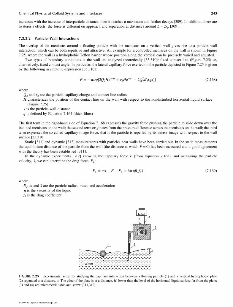
increases with the increase of interparticle distance, then it reaches a maximum and further decays [309]. In addition, there arehysteresis effects: the force is different on approach and separation at distances around L¼ 2rp [309].

7.3.3.2 Particle–Wall Interactions

The overlap of the meniscus around a floating particle with the meniscus on a vertical wall gives rise to a particle–wallinteraction, which can be both repulsive and attractive. An example for a controlled meniscus on the wall is shown in Figure7.25, where the wall is a hydrophobic Teflon barrier whose position along the vertical can be precisely varied and adjusted.

Two types of boundary conditions at the wall are analyzed theoretically [35,310]: fixed contact line (Figure 7.25) or,alternatively, fixed contact angle. In particular, the lateral capillary force exerted on the particle depicted in Figure 7.25 is givenby the following asymptotic expression [35,310]:

F ¼ �psq[2Q2He�qx þ r2He�qx � 2Q22K1(qx)] (7:168)

whereQ2 and r2 are the particle capillary charge and contact line radiusH characterizes the position of the contact line on the wall with respect to the nondisturbed horizontal liquid surface

(Figure 7.25)x is the particle–wall distanceq is defined by Equation 7.164 (thick films)

The first term in the right-hand side of Equation 7.168 expresses the gravity force pushing the particle to slide down over theinclined meniscus on the wall; the second term originates from the pressure difference across the meniscus on the wall; the thirdterm expresses the so-called capillary image force, that is the particle is repelled by its mirror image with respect to the wallsurface [35,310].

Static [311] and dynamic [312] measurements with particles near walls have been carried out. In the static measurementsthe equilibrium distance of the particle from the wall (the distance at which F¼ 0) has been measured and a good agreementwith the theory has been established [311].

In the dynamic experiments [312] knowing the capillary force F (from Equation 7.168), and measuring the particlevelocity, _x, we can determine the drag force, Fd:

Fd ¼ m€x� F, Fd � 6phR2fd _x (7:169)

whereR2, m and €x are the particle radius, mass, and accelerationh is the viscosity of the liquidfd is the drag coefficient

FIGURE 7.25 Experimental setup for studying the capillary interaction between a floating particle (1) and a vertical hydrophobic plate(2) separated at a distance, x. The edge of the plate is at a distance, H, lower than the level of the horizontal liquid surface far from the plate;(3) and (4) are micrometric table and screw [311,312].




4

3

2

H

1

x

Water

If the particle were in the bulk liquid, fd would be equal to 1 and Fd would be given by the Stokes formula. In general, fd differsfrom unity because the particle is attached to the interface. The experiment [312] gives fd varying between 0.68 and 0.54 forparticle contact angle varying from 498 to 828; the data are in good quantitative agreement with the hydrodynamic theory of thedrag coefficient [313]. In other words, the less the depth of particle immersion, the less the drag coefficient, as could beexpected. However, if the floating particle is heavy enough, it deforms the surrounding liquid surface; the deformation travelstogether with the particle, thus increasing fd several times [312]. The addition of surfactant strongly increases fd. The lattereffect can be used to measure the surface viscosity of adsorption monolayers from low molecular weight surfactants [314],which is not accessible to the standard methods for measurement of surface viscosity.

In the case of protein adsorption layers, the surface elasticity is so strong that the particle (Figure 7.25) is arrested in theadsorption film. Nevertheless, with heavier particles and at larger meniscus slopes, it is possible to break the protein adsorptionlayer. Based on such experiments, a method for determining surface elasticity and yield stress has been developed [315].

7.3.3.3 Electrically Charged Particles at Liquid Interfaces

7.3.3.3.1 Particle–Interface InteractionLet us consider a spherical dielectric particle (phase 1), which is immersed in a nonpolar medium (phase 2), near its boundary witha third dielectric medium (phase 3); see the inset in Figure 7.26. The interaction is due to electric charges at the particle surface.The theoretical problem has been solved exactly, in terms of Legendre polynomials, for arbitrary values of the dielectric constantsof the three phases, and expressions for calculating the interaction force, Fz, and energy, W, have been derived [316]:

Fz ¼ b23Q2

4«2(Rþ s)2fz, W ¼

ð1

s

Fzds ¼ b23Q2

4«2(Rþ s)w (7:170)

whereR is the particle radiuss is the distance between the particle surface and the fluid interface (inset in Figure 7.26)Q¼ 4pR2spn is the total charge at the boundary particle–nonpolar fluid, where spn is the respective surface-chargedensity

fz and w are the dimensionless force and energy coefficients, which, in general, depend on the parameters s=R, b12, andb23, where bij¼ («i� «j)=(«iþ «j); i, j¼ 1, 2, 3

«1, «2, and «3 are the dielectric constants of the respective phases

At long distances, s=R> 1, we have fz�w� 1, and then Equation 7.170 reduces to the expressions for the force and energy ofinteraction between a point charge Q with the interface between phases 2 and 3. This is the known image charge effect.Expressions that allow us to calculate fz and w for shorter distances (s=R< 1) are derived in Ref. [316].

105 Attraction750 nmR =1000 nm

500 nm

300 nm

200 nm

100 nm75 nm

50 nm

30 nm

104

103

Inte

ract

ion

ener

gy, –

W/(

kT)

102

101

100

10–2 10–1 100 101

Dimensionless distance, s/R102 103 104 105

z

R

sO

phase 1

phase 2phase 3

FIGURE 7.26 Plot of the interaction energy W (scaled with kT) versus the dimensionless distance, s=R, between a charged glass particle(phase 1) and a planar interface; phase 2 is tetradecane; phase 3 is water. The curves correspond to different particle radii, R, denoted inthe figure.




In Figure 7.26, numerical results for the particle–interface interaction energy, W, scaled by the thermal energy kT, areplotted versus the relative distance, s=R, for various values of the particle radius, R. The other parameter values correspond tothe following choice of the phases: phase 1 (the particle) is glass, phase 2 is tetradecane and phase 3 is water. The curves inFigure 7.26 describe a strong and long-range attraction between the particle and the interface. The interaction energy, W,becomes comparable, or smaller than the thermal energy kT for particle radius R< 30 nm. On the other hand, for R> 30 nm Wstrongly increases with the particle size (in Equation 7.170, Q2 � R4 at fixed surface charge density, spn), and reaches W� 105

kT for R¼ 1 mm at close contact. In addition, the range of the interaction also strongly increases, reaching s=R� 105 for R¼ 1mm. In general, this is a strong and long-range interaction [316]. For example, water drops could attract charged hydrophobicparticles dispersed in the oily phase, which would favor the formation of reverse particle-stabilized emulsions.

7.3.3.3.2 Forces of Electric Origin between Particles at a Liquid InterfaceFigure 7.27 shows two particles attached to the interface between water and a nonpolar fluid (oil, air). In general, the particlesexperience three forces of electric origin: FED, electrodipping force [317]; FER, direct electric repulsion between the twoparticles across the oil [318]; and FEC, electric-field-induced capillary attraction [319], which is termed electrocapillary force,ECF, for brevity. FED is normal to the oil–water interface and is directed toward the water phase. Physically, FED is a result ofthe electrostatic image-charge effect; see the previous section. FED is acting on each individual particle, while FER and FEC areinteraction forces between two (or more) particles. The presence of electric field leads to deformations in the fluid interfacearound the particles, which lead to the appearance of FEC. The three forces, FED, FER, and FEC, are separately considered below.

7.3.3.3.3 Electrodipping ForceAt equilibrium, the electrodipping force is counterbalanced by the interfacial tension force: FED¼ 2prcg sinc, where g is theinterfacial tension; rc is the radius of the contact line on the particle surface; and c is the meniscus slope angle at the contact line(Figure 7.27) [317,319]. Consequently, FED can be determined from the experimental values of rc, g, and c. This approach wasused to obtain the values of FED for silanized glass particles of radii 200–300 mm from photographs of these particles at an oil–water or air–water interface [317]. FED was found to be much greater than the gravitational force acting on these particles.

As an illustration, Figure 7.28 compares the profiles of the liquid menisci around a noncharged particle and a chargedparticle. The particles represent hydrophobized glass spheres of density rp¼ 2.5 g cm�3. The oil phase is purified soybean oil

FIGURE 7.27 Sketch of two electrically charged particles attached to an oil–water interface. FED is the electrodipping force, due to theimage-charge effect, that pushes the particles into water and deforms the fluid interface around the particles. FER is the direct electric repulsionbetween the two like-charged particles. FEC is the electrocapillary attraction, related to deformations in the fluid interface created by theelectric field.

FIGURE 7.28 Side-view photographs of hydrophobized spherical glass particles at the boundary water–soybean oil (no added surfactants).(a) Noncharged particle of radius R¼ 235 mm: the meniscus slope angle due to gravity is relatively small, c¼ 1.58. (b) Charged particle ofradius R¼ 274 mm: the experimental meniscus slope angle is c¼ 268 owing to the electrodipping force; if this electric force were missing, thegravitational slope angle would be only c¼ 1.98.




Oil (air)

Water

FER

R

FERFEC

0

FEC

FEDFEDL

2rc

rcg siny

g

ya q

y

(a)

Water

Soybeanoil

y =1.5�

(b)

Water

Soybeanoil

y = 26�

of density roil¼ 0.92 g cm�3. The oil–water interfacial tension is g¼ 30.5 mN m�1. Under these conditions, the calculatedsurface-tension force, 2prcg sinc, which counterbalances the gravitational force (particle weight minus the Archimedes force)corresponds to meniscus slope angle c¼ 1.58, and the deformation of the liquid interface caused by the particle is hardly visible(Figure 7.28a). In contrast, for the charged particle (Figure 7.28b), the meniscus slope angle is much greater, c¼ 268. This isdue to the fact that the interfacial-tension force, 2prcg sinc, has to counterbalance the electrodipping force, which pushes theparticle toward the water phase. Experimentally, it has been found that the angle c is insensitive to the concentration of NaCl inthe aqueous phase, which means that (in the investigated case) the electrodipping force is due to charges situated at the particle–oil interface [317,320]. With similar particles, the magnitude of FED at the air–water interface was found to be about six timessmaller than at the oil–water interface [317].

Theoretically, the electrodipping force, FED, can be calculated from the expression [320,321]:

FED ¼ (4p=«n)(spnR)2(1� cosa)f (u,«pn) (7:171)

where«n is the dielectric constant of the nonpolar fluid (oil, air)spn is the surface charge density at the boundary particle–nonpolar fluid«pn¼ «p=«n is the ratio of the respective two dielectric constantsa is a central angle, while u¼aþc is the contact angle (see Figure 7.27)

We could accurately calculate the dimensionless function f(u,«pn) by means of the relation f(u,«pn)¼ fR(u,«pn)=(1� cosu),where the function fR(u,«pn) is tabulated in Table 7.3 of Ref. [321] on the basis of the solution of the electrostatic boundaryproblem. The tabulated values can be used for a convenient computer calculation of fR(u,«pn) with the help of a four-pointinterpolation formula, Equation D.1 in Ref. [321]. From the experimental FED and Equation 7.171, we could determine thesurface charge density, spn, at the particle–oil and particle–air interface. Values of spn in the range from 20 to 70 mC m�2 havebeen obtained [317,320].

7.3.3.3.4 Direct Electric RepulsionInteractions of electrostatic origin were found to essentially influence the type of particle structures at oil–water [318,319,322–324] and air–water [325,326] interfaces. Two-dimensional hexagonal arrays of particles were observed, in which the distancebetween the closest neighbors was markedly greater than the particle diameter [318–327]. The existence of such structures wasexplained by the action of direct electrostatic repulsion between like charged particles. In many cases, the particle arrays areinsensitive to the concentration of electrolyte in the aqueous phase [318,322,323]. This fact, and the direct interparticle forcemeasurements by laser tweezers [322], lead to the conclusion that the electrostatic repulsion is due to charges at the particle–oil(or particle–air) interface, which give rise to electric repulsion across the nonpolar phase [318,322–325]. This repulsion isrelatively long-ranged because of the absence of a strong Debye screening of the electrostatic forces that is typical for theaqueous phase. Evidences about the presence of electric charges on the surface of solid particles dispersed in liquidhydrocarbons could be found also in earlier studies [328,329].

For a particle in isolation, the charges at the particle–nonpolar fluid interface create an electric field in the oil thatasymptotically resembles the electric field of a dipole (Figure 7.29). This field practically does not penetrate into the waterphase, because it is reflected by the oil–water boundary owing to the relatively large dielectric constant of water. For a single

FIGURE 7.29 Two particles attached to the boundary water–nonpolar fluid and separated at a center-to-center distance L. In the nonpolarfluid (oil, air), the electric field of each particle in isolation is asymptotically identical to the field of a dipole of moment pd. This field is createdby charges at the particle–nonpolar fluid interface.




Water

Nonpolar fluid (oil or air)

pd pdL

particle, the respective electrostatic problem is solved in Ref. [321]. The asymptotic behavior of the force of electrostaticrepulsion between two such particles–dipoles (Figure 7.29) is [321]:

FER ¼ 3p2d2«nL4

(R=L � 1) (7:172)

L is the center-to-center distance between the two particles; pd¼ 4pspnDR3sin3a is the effective particle dipole moment; as

before, R is the particle radius and spn is the electric charge density at the particle–nonpolar fluid interface; D¼D(a,«pn) is aknown dimensionless function, which can be calculated by means of Table 7.1 and Equation D.1 in Ref. [321]; «pn � «p=«n isthe ratio of the dielectric constants of the two phases. Equation 7.172 shows that FER asymptotically decays as 1=L4 like theforce between two point dipoles. However, at shorter distances, the finite size of the particle is expected to lead to a Coulombicrepulsion, FER �1=L2 [322–325].

7.3.3.3.5 Electrocapillary ForceIn their experiments with 1.5 mm colloidal spheres at the surfaces of water droplets in oil, Nikolaides et al. [319] observedindications about attraction between like-charged particles, and attributed the observed effect to the action of electric-field-induced capillary attraction. Their work provoked a considerable interest, because the latter force could play an important rolein the micrometer and submicrometer world [330], where the effect of the gravity-induced lateral capillary force (Section7.3.3.1) is negligible.

What concerns the theoretical description of FEC, a generally accepted theory is still missing. The problem about theinterplay of capillary and electric effects turned out to be rather complex. Controversial results have been reported based onthe application of different truncated asymptotic expansions or other perturbation procedures [331–334]. Different approacheshave lead to the conclusion that FEC is attractive, but it is still unclear whether FEC could prevail over FER under typicalexperimental conditions [335–337]. In the meantime, the number of experimental evidences about the action of attractive forcesbetween particles at fluid interfaces keeps increasing [324,325,338–341].

As mentioned earlier, the capillary forces between particles are due to the overlap of the deformations in the liquid interfacecreated by the particles. Hence, a necessary condition for the existence of electric-field-induced capillary force is the presenceof interfacial deformations created by the electric field. As demonstrated in Figure 7.28, this necessary condition can besatisfied. The deformation is due not only to the electrodipping forces that pushes the particle toward the water (and thatdetermines the value of the angle c), but also to the additional electric pressure (Maxwell stress) that is acting per unit area ofthe oil–water (or air–water) interface owing to the presence of electric field in the nonpolar fluid (see Figure 7.29)[317,319,320,342]. The direction of this electric force (per unit area) is from the water toward the nonpolar fluid.

The electric-field-induced deformation of a liquid interface around charged particles at the interface tetradecane-water hasbeen quantitatively examined in Ref. [320]. An example is given in Figure 7.30. Far from the particle, the interface is flat and

300

0

5

10

15

20

Ver

tical

dis

tanc

e, z

(m

m)

25Level of the horizontal interface far from the particle

Gravitational profile

Realprofile

R = 241 µm

q =114�

rc = 236 µm

NaCI

0.0 mM3.3 mM9.9 mM16.4 mM25.9 mM41.5 mM

400

Radial distance, r (mm)

500 700 1000

FIGURE 7.30 Profile of the oil (tetradecane)=water interface near the contact line of a charged glass particle, like that in Figure 7.28b: plotof experimental data from Ref. [320]; see Figure 7.27 for the notations. The dash-dot line shows the gravitational; profile calculated under theassumption that the particle is not charged. The difference between the real and the gravitational profiles represents the effect of electric fieldon the meniscus shape. The fact that the real (experimental) profile is insensitive to the concentration of NaCl in the water phase indicates thatthe electric charges are located at the particle–oil interface, so that the interfacial deformation is due to electric field in the oily phase.




horizontal. For particles of radii R¼ 200–300 mm, both gravitational and electric field induced deformations are present. Thegravitational deformation is predominant at longer distances, whereas the electric-field deformation is significant near theparticle. The latter deformation is insensitive to the variation of the concentration of NaCl in the aqueous phase (Figure 7.30),which indicates that this deformation is due to electric charges at the particle–oil interface. Good agreement betweenexperiment (the symbols) and theory (the solid line) has been obtained.

In Ref. [343], the motion of spherical glass particles of radii 240–310 mm attached to a tetradecane–water interface wasinvestigated. Couples of particles, which were moving toward each other under the action of lateral capillary force, are observedby optical microscopy. The analysis of the experimental results, including the comparison of the motion of charged andnoncharged particles, evidences for the existence of an additional attraction between two like-charged particles at the oil–waterinterface. This attraction exceeds the direct electrostatic repulsion between the two particles and leads to a noticeableacceleration of their motion [343].

7.4 SURFACE FORCES

7.4.1 DERJAGUIN APPROXIMATION

The excess surface free energy per unit area of a plane-parallel film of thickness h is [14,344]

f (h) ¼ð1

h

P(h) dh (7:173)

where, as before, P denotes disjoining pressure. Derjaguin [345] derived an approximate formula, which expresses the energyof interaction between two spherical particles of radii R1 and R2 through integral of f(h):

U(h0) ¼ 2pR1R2

R1 þ R2

ð1

h0

f (h) dh (7:174)

where h0 is the shortest distance between the surfaces of the two particles (see Figure 7.31). In the derivation of Equation 7.174it is assumed that the interaction between two parcels from the particle surfaces, separated at the distance h, is approximately thesame as that between two similar parcels in a plane-parallel film. This assumption is correct when the range of action of thesurface forces and the distance h0 are small compared to the curvature radii R1 and R2. It has been established, bothexperimentally [34] and theoretically [346], that Equation 7.174 provides a good approximation in the range of its validity.

Equation 7.174 can be generalized for smooth surfaces of arbitrary shape (not necessarily spheres). For that purpose, thesurfaces of the two particles are approximated with paraboloids in the vicinity of the point of closest approach (h¼ h0). Let theprinciple curvatures at this point be c1 and c01 for the first particle, and c2 and c02 for the second particle. Then the generalizationof Equation 7.174 reads [344]:

U(h0) ¼ 2pffiffiffiffiC

pð1

h0

f (h) dh (7:175)

R1R2

h0

h

FIGURE 7.31 Two spherical particles of radii R1 and R2; the shortest and the running surface-to-surface distances are denoted by h0 and h,respectively.




C � c1c01 þ c2c

02 þ (c1c2 þ c01c

02) sin

2 vþ (c1c02 þ c01c2) cos

2 v

where v is the angle subtended between the directions of the principle curvatures of the two approaching surfaces. For twospheres, we have c1 ¼ c01 ¼ 1=R1, c2 ¼ c02 ¼ 1=R2, and Equation 7.175 reduces to Equation 7.174.

For two cylinders of radii r1 and r2 crossed at angle v we have c1¼ c2¼ 0; c01 ¼ 1=r1, c02 ¼ 1=r2 and Equation 7.175 yields

U(h0) ¼ 2pffiffiffiffiffiffiffiffir1r2

psinv

ð1

h0

f (h) dh (7:176)

Equation 7.176 is often used in connection to the experiments with the surface force apparatus [34,347], in which theinteracting surfaces are two crossed cylindrical mica sheets. The divergence in Equation 7.176 for v¼ 0 reflects the fact thatthe axes of the two infinitely long cylinders are parallel for v¼ 0 and thus the area of the interaction zone becomes infinite.

The main features of the Derjaguin approximation are the following: (1) It is applicable to any type of force law (attractive,repulsive, oscillatory), if the range of the forces is much smaller than the particles radii and (2) It reduces the problem forinteractions between particles to the simpler problem for interactions in plane-parallel films.

7.4.2 VAN DER WAALS SURFACE FORCES

The van der Waals interaction between molecules i and j obeys the law:

uij(r) ¼ �aij

r6(7:177)

whereuij is the potential energy of interactionr is the distance between the two moleculesaij is a constant characterizing the interaction

In fact, the van der Waals forces represent an averaged dipole–dipole interaction, which is a superposition of three main terms:(1) orientation interaction: interaction between two permanent dipoles [348]; (2) induction interaction: interaction betweenone permanent dipole and one induced dipole [349]; (3) dispersion interaction: interaction between two induced dipoles [350].The theory yields [34]:

aij ¼ 1

(4p«0)2p2i p

2j

3kTþ ( p2i a0j þ p2j a0i)þ 3a0ia0jhpninj

2(ni þ nj)

" #(7:178)

wherepi and ai0 are the molecular dipole moment and electronic polarizabilityhp is the Planck constantni is the orbiting frequency of the electron in the Bohr atom

For van der Waals interactions between molecules in a gas phase, the orientation interaction can yield from 0% (nonpolarmolecules) up to 70% (molecules of large permanent dipole moment, like H2O) of the value of aij; the contribution of theinduction interaction in aij is usually low, about 5%–10%; the contribution of the dispersion interaction might be between 24%(water) and 100% (nonpolar hydrocarbons) (for numerical data, see Ref. [34]).

According to the microscopic theory by Hamaker [351], the van der Waals interaction between two macroscopic bodies canbe found by integration of Equation 7.177 over all couples of molecules, followed by subtraction of the interaction energy atinfinite separation between the bodies. The result depends on the geometry of the system. For a plane-parallel film fromcomponent 3 located between two semiinfinite phases composed from components 1 and 2, the van der Waals interactionenergy per unit area and the respective disjoining pressure, stemming from Equation 7.177, are [351]:

fvw ¼ � AH

12ph2, Pvw ¼ � @fvw

@h¼ � AH

6ph3(7:179)




where, as usual, h is the thickness of the film and AH is the compound Hamaker constant [14]:

AH ¼ A33 þ A12 � A13 � A23 (Aij ¼ p2rirjaij, i, j ¼ 1,2,3) (7:180)

Aij is the Hamaker constant of components i and j; ri and rj are the molecular number densities of phases i and j built up fromcomponents i and j, respectively. If Aii and Ajj are known, we can calculate Aij by using the Hamaker approximation

Aij ¼ (AiiAjj)1=2 (7:181)

In fact, Equation 7.181 is applicable to the dispersion contribution in the van der Waals interaction [34].When components 1 and 2 are identical, AH is positive (see Equation 7.180), therefore, the van der Waals interaction

between identical bodies, in any medium, is always attractive. Besides, two dense bodies (even if nonidentical) will attract eachother when placed in medium 3 of low density (gas, vacuum). When the phase in the middle (component 3) has intermediateHamaker constant between those of bodies 1 and 2, AH can be negative and the van der Waals disjoining pressure can berepulsive (positive). Such is the case of an aqueous film between mercury and gas [352].

Lifshitz et al. [353,354] developed an alternative approach to the calculation of the Hamaker constant AH in condensedphases, called the macroscopic theory. The latter is not limited by the assumption for pairwise additivity of the van der Waalsinteraction [34,344,355]. The Lifshitz theory treats each phase as a continuous medium characterized by a given uniformdielectric permittivity, which is dependent on the frequency, n, of the propagating electromagnetic waves. For the symmetricconfiguration of two identical phases i interacting across a medium j, the macroscopic theory provides the expression [34]

AH � Aiji ¼ A(n¼0)iji þ A(n>0)

iji ¼ 34kT

«i � «j«i þ «j

� �2

þ 3hpne(n2i � n2j )2

16ffiffiffi2

p(n2i þ n2j )

3=2(7:182)

where«i and «j are the dielectric constants of phases i and j; ni and nj are the respective refractive indices for visible lighthp is the Planck constantne is the main electronic absorption frequency which is�3.0�1015 Hz for water and the most organic liquids [34]

The first term in the right-hand side of Equation 7.182, A(n¼0)iji , is the so-called zero-frequency term, expressing the contribution

of the orientation and induction interactions. Indeed, these two contributions to the van der Waals force represent electrostaticeffects. Equation 7.182 shows that the zero-frequency term can never exceed 3=4kT� 3� 10�21 J. The last term in Equation7.182, A(n>0)

iji , accounts for the dispersion interaction. If the two phases, i and j, have comparable densities (as for emulsionsystems, say oil–water–oil), then A(n>0)

iji and A(n¼0)iji are comparable by magnitude. If one of the phases, i or j, has a low density

(gas, vacuum), we obtain A(n>0)iji � A(n¼0)

iji . In the latter case, the Hamaker microscopic approach may give comparable A(n>0)iji

and A(n¼0)iji in contradiction to the Lifshitz macroscopic theory, which is more accurate for condensed phases.

A geometrical configuration, which is important for disperse systems, is the case of two spheres of radii R1 and R2

interacting across a medium (component 3). Hamaker [351] has derived the following expression for the van der Waalsinteraction energy between two spheres:

U(h0) ¼ �AH

12y

x2 þ xyþ xþ y

x2 þ xyþ xþ yþ 2 ln

x2 þ xyþ x

x2 þ xyþ xþ y

� �(7:183)

where

x ¼ h0=2R1, y ¼ R2=R1 � 1 (7:184)

and h0 is the same as in Figure 7.31. For x � 1 Equation 7.183 reduces to

U(h0) � �AH

12y

(1þ y)x¼ � 2pR1R2

R1 þ R2

AH

12ph0(7:185)

Equation 7.185 can be also derived by combining Equation 7.179 with the Derjaguin approximation (Equation 7.174). It isworthwhile noting, that the logarithmic term in Equation 7.183 can be neglected only if x � 1. For example, even whenx¼ 5� 10�3, the contribution of the logarithmic term amounts to about 10% of the result (for y¼ 1); consequently, for largervalues of x this term must be retained.




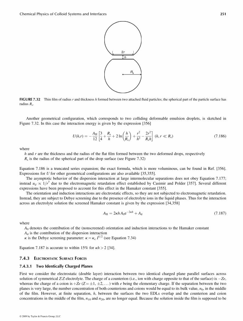
Another geometrical configuration, which corresponds to two colliding deformable emulsion droplets, is sketched inFigure 7.32. In this case the interaction energy is given by the expression [356]

U(h,r) ¼ �AH

1234þ Rs

hþ 2 ln

h

Rs

� �þ r2

h2� 2r2

Rsh

� �(h, r � Rs) (7:186)

whereh and r are the thickness and the radius of the flat film formed between the two deformed drops, respectivelyRs is the radius of the spherical part of the drop surface (see Figure 7.32)

Equation 7.186 is a truncated series expansion; the exact formula, which is more voluminous, can be found in Ref. [356].Expressions for U for other geometrical configurations are also available [35,355].

The asymptotic behavior of the dispersion interaction at large intermolecular separations does not obey Equation 7.177;instead uij / 1=r7 due to the electromagnetic retardation effect established by Casimir and Polder [357]. Several differentexpressions have been proposed to account for this effect in the Hamaker constant [355].

The orientation and induction interactions are electrostatic effects, so they are not subjected to electromagnetic retardation.Instead, they are subject to Debye screening due to the presence of electrolyte ions in the liquid phases. Thus for the interactionacross an electrolyte solution the screened Hamaker constant is given by the expression [34,358]

AH ¼ 2kh A0e�2kh þ Ad (7:187)

whereA0 denotes the contribution of the (nonscreened) orientation and induction interactions to the Hamaker constantAd is the contribution of the dispersion interactionk is the Debye screening parameter: k¼ kc I

1=2 (see Equation 7.34)

Equation 7.187 is accurate to within 15% for kh> 2 [34].

7.4.3 ELECTROSTATIC SURFACE FORCES

7.4.3.1 Two Identically Charged Planes

First we consider the electrostatic (double layer) interaction between two identical charged plane parallel surfaces acrosssolution of symmetrical Z:Z electrolyte. The charge of a counterion (i.e., ion with charge opposite to that of the surface) is �Ze,whereas the charge of a coion isþZe (Z¼�1, �2, . . . ) with e being the elementary charge. If the separation between the twoplanes is very large, the number concentration of both counterions and coions would be equal to its bulk value, n0, in the middleof the film. However, at finite separation, h, between the surfaces the two EDLs overlap and the counterion and coionconcentrations in the middle of the film, n10 and n20, are no longer equal. Because the solution inside the film is supposed to be

2r

Rs

h

FIGURE 7.32 Thin film of radius r and thickness h formed between two attached fluid particles; the spherical part of the particle surface hasradius Rs.




in electrochemical (Donnan) equilibrium with the bulk electrolyte solution of concentration n0, we can write [359] n10n20 ¼ n20,or alternatively

n10 ¼ n0=ffiffiffiffim

p, n20 ¼ n0

ffiffiffiffim

p, m � n20=n10 (7:188)

As pointed out by Langmuir [360], the electrostatic disjoining pressure, Pel, can be identified with the excess osmotic pressurein the middle of the film:

Pel ¼ kT(n10 þ n20 � 2n0) ¼ n0kT(m1=4 � m�1=4)2 (7:189)

Equation 7.189 demonstrates that for two identically charged surfaces Pel, is always positive, i.e., corresponds to repulsionbetween the surfaces. In general, we have 0<m �1, because the coions are repelled from the film due to the interaction withthe film surfaces. To find the exact dependence of Pel on the film thickness, h, we have to solve the Poisson–Boltzmannequation for the distribution of the electrostatic potential inside the film. The solution provides the following connectionbetween Pel and h for symmetric electrolytes [344,361]:

Pel ¼ 4n0kT cot2 u, kh ¼ 2F(w,u) sin u (7:190)

where F(w,u) is an elliptic integral of the first kind, and w is related with u as follows:

cosw ¼ cotu

sinhZFs

2

� � (fixed surface potential Fs) (7:191)

tanw ¼ (tan u)sinhZF12

� �(fixed surface charge ss) (7:192)

cosh(ZF1) ¼ 1þ 12

Zess

««0kTk

� �2

, Fs � ecs

kT(7:193)

whereFs is the dimensionless surface potentialF1 is the value of Fs for h ! 1

Equation 7.190 expresses the dependence Pel(h) in a parametric form: Pel(u), h(u). Fixed surface potential or charge meansthat Fs or ss does not depend on the film thickness h. The latter is important to be specified when integrating P(h) or f(h)(in accordance with Equations 7.173 or 7.176) to calculate the interaction energy.

In principle, it is possible neither the surface potential nor the surface charge to be constant [362]. In such case a conditionfor charge regulation is applied, which in fact represents the condition for dynamic equilibrium of the counterion exchangebetween the Stern and diffuse parts of the EDL (i.e., condition for constant electrochemical potentials of the ionic species). Asdiscussed in Section 7.2.1.2.3, the Stern layer itself can be considered as a Langmuir adsorption layer of counterions. We canrelate the maximum possible surface charge density (due to all surface ionizable groups) to G1 in Equation 7.47: smax¼ ZeG1.Likewise, the effective surface charge density, ss, which is smaller by magnitude than smax (because some ionizable groups areblocked by adsorbed counterions) can be expressed as ss¼ Ze(G1�G2). Then, with the help of Equation 7.44, the Sternisotherm (Equation 7.47) can be represented in the form

smax � ss

smax

¼ [1þ (K2I)�1 exp (ZFs)]

�1 (7:194)

The product ZFs is always positive. At high surface potential, ZFs !1, from Equation 7.194 we obtain ss ! smax, i.e., thereis no blocking of surface ionizable groups by adsorbed counterions.

When the film thickness is large enough (kh � 1) the difference between the regimes of constant potential, constant chargeand charge regulation becomes negligible, i.e., the usage of each of them leads to the same results for Pel(h) [14].

When the dimensionless electrostatic potential in the middle of the film

Fm ¼ e

kTcm ¼ � 1

2Zlnm (7:195)




is small enough (the film thickness, h, is large enough), we could use the superposition approximation, i.e., we could assumethat Fm� 2F1(h=2), where F1 is the dimensionless electric potential at a distance h=2 from the surface (of the film) when theother surface is removed at infinity. Because

ZF1(h=2) ¼ 4e�kh=4 tanh(ZFs=4) (7:196)

from Equations 7.189, 7.195, and 7.196 we obtain a useful asymptotic formula [363]

Pel � n0kTZ2F2

m � 64n0kT tanhZFs

4

� �2

e�kh (7:197)

It should be noted that if Fs is large enough, the hyperbolic tangent in Equation 7.197 is identically 1, and Pel (as well as fel)becomes independent of the surface potential (or charge). Equation 7.197 can be generalized for the case of 2:1 electrolyte(bivalent counterion) and 1:2 electrolyte (bivalent coion) [364]:

Pel ¼ 432n(2)kT tanhvi:j4

� �2e�kh (7:198)

where n(2) is the concentration of the bivalent ions, the subscript i:j takes the value 2:1 or 1:2, and

v2:1 ¼ ln [3=(1þ 2e�Fs )], v1:2 ¼ ln [(2eFs þ 1)=3] (7:199)

7.4.3.2 Two Nonidentically Charged Planes

Contrary to the case of two identically charged surfaces, which always repel each other (see Equation 7.189), the electrostaticinteraction between two plane-parallel surfaces of different potentials, cs1 and cs2, can be either repulsive or attractive[344,365]. Here, we will restrict our considerations to the case of low surface potentials, when the Poisson–Boltzmann equationcan be linearized. Despite that it is not too general quantitatively, this case exhibits qualitatively all features of the electrostaticinteraction between different surfaces.

If cs1¼ constant, and cs2¼ constant, then the disjoining pressure at constant surface potential reads [344]:

Pcel ¼

««0k2

2p2cs1cs2 coshkh� (c2

s1 þ c2s2)

sinh2kh(7:200)

When the two surface potentials have opposite signs, i.e., when cs1cs2 < 0, Pcel is negative for all h and corresponds to

electrostatic attraction (see Figure 7.33a). This result could have been anticipated, because two charges of opposite sign attracteach other. More interesting is the case, when cs1cs2> 0, but cs1 6¼ cs2. In the latter case, the two surfaces repel each other for

0

(a) (b)

0

2 2

1

+

+

Πel Πel

Πmax

Πmin

ys1ys2 < 0

ys1ys2 > 0 ss1ss2 > 0

ss1ss2 < 0

++

+++

+++

+++

+++

+ −−−−

−−−−

+++

1

h0h h

h0

hmax

hmin

y

y

s

s

FIGURE 7.33 Electrostatic disjoining pressure at (a) fixed surface potential, Pcel, and (b) fixed surface charge density, Ps

el, both of themplotted versus the film thickness h. cs1 and cs2 are the potentials of the two surfaces; ss1 and ss2 are the respective surface charge densities.




h> h0, whereas they attract each other for h< h0 (Figure 7.33a); h0 is determined by the equation kh0¼ ln (cs2=cs1); cs2>cs1.In addition, the electrostatic repulsion has a maximum value of

Pcel( max ) ¼ ««0k

2

2pc2s1 at hmax ¼ 1

karccosh

cs2

cs1

, cs2 > cs1 (7:201)

Similar electrostatic disjoining pressure isotherm has been used to interpret the experimental data for aqueous films on mercury[147]. It is worthwhile noting, thatPc

el (max) depends only on cs1, i.e., the maximum repulsion is determined by the potential ofthe surface of lower charge.

If ss1¼ constant, and ss2¼ constant, then instead of Equation 7.200 we have [344]

Psel(h) ¼

12««0

2ss1ss2 coshkhþ s2s1 þ s2

s2

sinh2kh(7:202)

When s1s2> 0 Equation 7.202 yields Psel > 0 for every h (see Figure 7.33b). However, when s1s2 < 0, Ps

el is repulsivefor small thickness, h< h0 and attractive for larger separations, h> h0; h0 is determined by the equation kh0 ¼ ln (�ss2=ss1);jss2j > jss1j. The electrostatic disjoining pressure in this case has a minimum value

Psel( min ) ¼ 1

««0ss1ss2, at hmin ¼ 1

karccosh �ss2

ss1

� �(7:203)

Finally, it should be noted, that all curves depicted in Figure 7.24 decay exponentially at h!1. An asymptotic expression forZ:Z electrolytes, which generalizes Equation 7.197, holds [344,363]:

Pel(h) ¼ 64n0kTg1g2e�kh, gk � tanh

Zecsk

4kT

� �, k ¼ 1, 2 (7:204)

Equation 7.204 is valid for both low and high surface potentials, only if exp(�kh) � 1.

7.4.3.3 Two Charged Spheres

When the EDLs are thin compared with the particle radii (k�1 � R1, R2) and the gap between the particles is small (h0 � R1,R2), we can use Equation 7.204 in conjunction with the Derjaguin approximation, Equations 7.173 and 7.174. The result for theenergy of electrostatic interaction between two spheres reads:

Uel(h0) ¼ 128pR1R2

k2(R1 þ R2)n0kTg1g2e

�kh (7:205)

Equation 7.205 is valid for any surface potentials cs1 and cs2 but only for exp(kh)� 1. Complementary expressions, which arevalid for every h� R1,R2, but for small surface potentials, can be derived by integrating Equations 7.200 and 7.202, instead ofEquation 7.204. In this way, for cs1¼ constant and cs2¼ constant, we can derive [366]:

Ucel(h0) ¼

p««0R1R2

R1 þ R2[(cs1 þ cs2)

2 ln (1þ e�kh0)þ (cs1 � cs2)2 ln (1� e�kh0)] (7:206)

or, alternatively, for ss1¼ constant and ss2¼ constant we obtain [367]

Usel(h0) ¼

�pR1R2

««0k2(R1 þ R2)[(ss1 þ ss2)

2 ln (1� e�kh0)þ (ss1 � ss2)2 ln (1þ e�kh0)] (7:207)

The range of validity of the different approximations involved in the derivations of Equations 7.205 through 7.207 is discussedin the book by Russel et al. [368]

As mentioned above, Equations 7.205 through 7.207 hold for h0 � R. In the opposite case, when h0 is comparable to orlarger than the particle radius R, we can use the equation [14]

Uel(h0) ¼ 4p««0c2sR

2

2Rþ h0e�kh0 (7:208)




stemming from the theory of Debye and Hückel [369] for two identical particles. Equation 7.208 was derived by using thesuperposition approximation (valid for weak overlap of the two EDLs) and the linearized Poisson–Boltzmann equation. Asimple approximate formula, representing in fact interpolation between Equations 7.208 and 7.206 (the latter for R1¼R2¼R),has been derived by McCartney and Levine [370]

Ucel(h0) ¼ 4p««0Rc

2s

Rþ h02Rþ h0

ln 1þ Re�kh0

Rþ h0

� �(7:209)

Equation 7.209 has the advantage to give a good approximation for every h0 provided that the Poisson–Boltzmann equationcan be linearized. Similar expressions for the energy of electrostatic interaction between two deformed droplets or bubbles(Figure 7.32) can be derived [356].

7.4.4 DERJAGUIN–LANDAU–VERWEY–OVERBEEK (DLVO) THEORY

The first quantitative theory of interactions in thin liquid films and dispersions is the DLVO theory called after the names of theauthors: Derjaguin and Landau [371] and Verwey and Overbeek [363]. In this theory, the total interaction is supposed to be asuperposition of van der Waals and double layer interactions. In other words, the total disjoining pressure and the totalinteraction energy are presented in the form:

P ¼ Pvw þPel, U ¼ Uvw þ Uel (7:210)

A typical curve, P versus h, exhibits a maximum representing a barrier against coagulation, and two minima, called primaryand secondary minimum (see Figure 7.17); the U versus h curve has a similar shape. The primary minimum appears if strongshort-range repulsive forces (e.g., steric forces) are present. With small particles, the depth of the secondary minimum is usuallysmall (Umin< kT). If the particles cannot overcome the barrier, coagulation (flocculation) does not take place, and the dispersionis stable due to the electrostatic repulsion, which gives rise to the barrier. With larger colloidal particles (R> 0.1 mm) thesecondary minimum could be deep enough to cause coagulation and even formation of ordered structures of particles [372].

By addition of electrolyte or by decreasing the surface potential of the particles, we can suppress the electrostatic repulsionand thus decrease the height of the barrier. According to DLVO theory, the critical condition determining the onset of rapidcoagulation is

U(hmax) ¼ 0,dU

dh

hmax

¼ 0 (7:211)

where h¼ hmax denotes the position of the barrier.By using Equation 7.185 for Uvw and Equation 7.205 for Uel we derive from Equations 7.210 and 7.211 the following

criterion for the threshold of rapid coagulation of identical particles (R1¼R2¼R; g1¼ g2¼ g):

k6

n20¼ 768p

AH

kTe�1 tanh2Zecs

4kT

� �� 2(7:212)

For a Z:Z electrolyte, substituting k2¼ (2Z2e2n0)=(«0«kT) into Equation 7.212, we obtain:

n0(critical) / 1Z6

tanh4Zecs

4kT

� �(7:213)

When cs is high enough, the hyperbolic tangent equals 1 and Equation 7.213 yields n0(critical) / Z�6 which is, in fact, theempirical rule established earlier by Schulze [373] and Hardy [374].

7.4.5 NON-DLVO SURFACE FORCES

After 1980, a number of surface forces have been found out which are not taken into account by conventional DLVO theory.They are considered separately below.

7.4.5.1 Ion Correlation Forces

As shown by Debye and Hückel [369], due to the strong electrostatic interaction between the ions in a solution, the positions ofthe ions are correlated in such a way that a counterion atmosphere appears around each ion, thus screening its Coulomb




potential. The energy of formation of the counterion atmospheres gives a contribution to the free energy of the system calledcorrelation energy [23]. The correlation energy affects also a contribution to the osmotic pressure of the electrolyte solution,which can be presented in the form [23]

Posm ¼ kTXki¼1

ni � kTk2

24p(7:214)

The first term in the right-hand side of the Equation 7.214 corresponds to an ideal solution, whereas the second term takes intoaccount the effect of electrostatic interactions between the ions (the same effect is accounted for thermodynamically by theactivity coefficient, see Equation 7.31).

The expression forPel in the DLVO theory (Equation 7.189) obviously corresponds to an ideal solution, the contribution ofthe ionic correlations being neglected. Hence, in a more general theory instead of Equation 7.210 we could write:

P ¼ Pvw þPel þPcor (7:215)

where Pcor is the contribution of the ionic correlations to the disjoining pressure. The theory of Pcor takes into account thefollowing effects: (1) the different ionic concentration (and hence the different Debye screening) in the film compared to that inthe bulk solution; (2) the energy of deformation of the counterion atmosphere due to the image forces; (3) the energy of thelong-range correlations between charge-density fluctuations in the two opposite EDLs. For calculating Pcor both numericalsolutions [375,376] and analytical expressions [377–379] have been obtained. For example, in the case when the electrolyte issymmetrical (Z:Z) and exp(�kh) � 1 we can use the asymptotic formula [377]

Pcor ¼ Pel

Z2e2k

16p««0kT( ln 2þ 2IC)þ O(e�kh) (7:216)

where Pel is the conventional DLVO electrostatic disjoining pressure,

IC ¼ 12(1þ J) ln 2þ 2� 2z3 þ z

2z(2z2 � 1)2� 12(1� J) ln (zþ z2)

�ffiffiffiffiffiffiffiffiffiffiffiffiz2 � 1

p

z[1þ J þ 4(2z2 � 1)�3] arctan

ffiffiffiffiffiffiffiffiffiffiffiz� 1zþ 1

r

J � 2z2 � 3

(2z2 � 1)3, z � 1þ ess

2««0kTk

� �2" #1=2

The results for the case of symmetric electrolytes are the following. Pcor is negative and corresponds to attraction, which can becomparable by magnitude with Pvw. In the case of 1:1 electrolyte Pcor is usually a small correction to Pel. In the case of 2:2electrolyte, however, the situation can be quite different: the attractive forces, PcorþPvw, prevails over Pel and the totaldisjoining pressure, P, becomes negative. The effect of Pcor is even larger in the presence of ions of higher valence. Short-range net attractive ion-correlation forces have been measured by Marra [380,381] and Kjellander et al. [382,383] betweenhighly charged anionic bilayer surfaces in CaCl2 solutions. These forces are believed to be responsible for the strong adhesionof some surfaces (clay and bilayer membranes) in the presence of divalent counterions [34,382,384]. On the other hand,Kohonen et al. [385] measured a monotonic repulsion between two mica surfaces in 4.8� 10�3 M solution of MgSO4.Additional work is necessary to verify the theoretical predictions and to clarify the physical significance of the ion-correlationsurface force.

Note that the theory predicts ion-correlation attraction not only across water films with overlapping EDLs, but also acrossoily films intervening between two water phases. In the latter case, Pcor is not zero because the ions belonging to the two outerdouble layers interact across the thin dielectric (oil) film. The theory for such a film [386] predicts that Pcor is negative(attractive) and strongly dependent on the dielectric permittivity of the oil film;Pcor can be comparable by magnitude withPvw;Pel¼ 0 in this case.

7.4.5.2 Steric Interaction

7.4.5.2.1 Physical BackgroundThe steric interaction between two surfaces appears when chain molecules, attached at some point(s) to a surface, dangle outinto the solution (see Figure 7.34). When two such surfaces approach each other, the following effects take place [34,387–389]:




(1) The entropy decreases due to the confining of the dangling chains which results in a repulsive osmotic force known as stericor overlap repulsion. (2) In a poor solvent, the segments of the chain molecules attract each other; hence the overlap of the twoapproaching layers of polymer molecules will be accompanied with some intersegment attraction; the latter can prevail forsmall overlap, however at the distance of larger overlap it becomes negligible compared with the osmotic repulsion. (3) Anothereffect, known as the bridging attraction, occurs when two opposite ends of chain molecule can attach (adsorb) to the oppositeapproaching surfaces, thus forming a bridge between them (see Figure 7.34e).

Steric interaction can be observed in foam or emulsion films stabilized with nonionic surfactants or with various polymers,including proteins. The usual nonionic surfactants molecules are anchored (grafted) to the liquid interface by their hydrophobicmoieties. When the surface concentration of adsorbed molecules is high enough, the hydrophilic chains are called to form abrush (Figure 7.34b). The coils of macromolecules, like proteins, can also adsorb at a liquid surface (Figure 7.34c). Sometimesthe configurations of the adsorbed polymers are very different from the statistical coil: loops, trains, and tails can bedistinguished (Figure 7.34d).

The osmotic pressure of either dilute or concentrated polymer solutions can be expressed in the form [390]:

Posm

nkT¼ 1

Nþ 12nvþ 1

3n2wþ (7:217)

whereN is the number of segments in the polymer chainn is the number segment densityv and w account for the pair and triplet interactions, respectively, between segments

In fact, v and w are counterparts of the second and third virial coefficients in the theory of imperfect gases [11]; v and w can becalculated if information about the polymer chain and the solvent is available [368]:

w1=2 ¼ vm=NA, v ¼ w1=2(1� 2x) (7:218)

wherev (m3=kg) is the specific volume per segmentm (kg=mol) is the molecular weight per segmentNA is the Avogadro numberx is the Flory parameter

The latter depends on both the temperature and the energy of solvent–segment interaction. Then, v can be zero (see Equation7.218) for some special temperature, called the theta temperature. The solvent at the theta temperature is known as the thetasolvent or ideal solvent. The theta temperature in polymer solutions is a counterpart of the Boil temperature in imperfect gases:this is the temperature at which the intermolecular (intersegment) attraction and repulsion are exactly counterbalanced. In a

Loop

Brush

(a)

L

(d) (e)

(b) (c)

Tail

Train

FIGURE 7.34 Polymeric chains adsorbed at an interface: (a) terminally anchored polymer chain of mean end-to-end distance L; (b) a brushof anchored chains; (c) adsorbed (but not anchored) polymer coils; (d) configuration with a loop, trains and tails; (e) bridging of two surfacesby adsorbed polymer chains.




good solvent, however, the repulsion due mainly to the excluded volume effect dominates the attraction and v> 0. In contrast,in a poor solvent the intersegment attraction prevails, so v< 0.

7.4.5.2.2 Thickness of the Polymer Adsorption LayerThe steric interaction between two approaching surfaces appears when the film thickness becomes of the order of, or smallerthan 2L where L is the mean-square end-to-end distance of the hydrophilic portion of the chain. If the chain was entirelyextended, then L would be equal to Nl with l being the length of a segment; however, due to the Brownian motion L<Nl. Foran anchored chain, like that depicted in Figure 7.34a, in a theta solvent, L can be estimated as [368]:

L � L0 � lffiffiffiffiN

p(7:219)

In a good solvent L> L0, whereas in a poor solvent L< L0. In addition, L depends on the surface concentration, G, of theadsorbed chains, i.e., L is different for an isolated molecule and for a brush (see Figures 7.34a and b). The mean field approach[368,391] applied to polymer solutions provides the following equation for calculating L

eL3 � 1þ 19eG2

� �eL�1 ¼ 1

6ev (7:220)

where eL, eG, and ev are the dimensionless values of L, G, and v defined as follows:

eL ¼ L=(lffiffiffiffiN

p), eG ¼ GN

ffiffiffiffiw

p=l, ev ¼ vGN3=2=l (7:221)

For an isolated adsorbed molecule (eG ¼ 0) in an ideal solvent (ev ¼ 0) Equation 7.220 predicts eL ¼ 1, i.e., L¼ L0.

7.4.5.2.3 Overlap of Adsorption LayersWe now consider the case of terminally anchored chains, like those depicted in Figures 7.34a and b. Dolan and Edwards [392]calculated the steric interaction free energy per unit area, f, as a function on the film thickness, h, in a theta solvent:

f (h) ¼ GkTp2

3L20h2

� ln8p3

L20h2

� �� for h < L0

ffiffiffi3

p(7:222)

f (h) ¼ 4GkT exp � 3h2

2L20

� �for h > L0

ffiffiffi3

p(7:223)

where L0 is the end-to-end distance as defined by Equation 7.219. The boundary between the power-law regime ( f / 1=h2) andthe exponential decay regime is at h ¼ L0

ffiffiffi3

p � 1:7L0, the latter being slightly less than 2L0, which is the intuitively expectedonset of the steric overlap. The first term in the right-hand side of Equation 7.222 comes from the osmotic repulsion between thebrushes, which opposes the approach of the two surfaces; the second term is negative and accounts effectively for the decreaseof the elastic energy of the initially extended chains when the thickness of each of the two brushes, pressed against each other,decreases.

In the case of good solvent the disjoining pressure P¼�df=dh can be calculated by means of Alexander-de Gennes theoryas [393,394]:

P(h) ¼ kTG3=2 2Lgh

� �9=4

� h

2Lg

� �3=4" #

for h < 2Lg, Lg ¼ N(Gl5)1=3 (7:224)

where Lg is the thickness of a brush in a good solvent [395]. The positive and the negative terms in the right-hand side ofEquation 7.224 correspond to osmotic repulsion and elastic attraction. The validity of Alexander-de Gennes theory wasexperimentally confirmed by Taunton et al. [396] who measured the forces between two brush layers grafted on the surfaces oftwo crossed mica cylinders.

In the case of adsorbed molecules, like these in Figure 7.34c, which are not anchored to the surface, the measured surfaceforces depend significantly on the rate of approaching of the two surfaces [397,398]. The latter effect can be attributed to thecomparatively low rate of exchange of polymer between the adsorption layer and the bulk solution. This leads to a hysteresis ofthe surface force: different interaction on approach and separation of the two surfaces [34]. In addition, we can observe tworegimes of steric repulsion: (1) weaker repulsion at larger separations due to the overlap of the tails (Figure 7.34d) and (2)stronger repulsion at smaller separations indicating overlap of the loops [399].




7.4.5.3 Oscillatory Structural Forces

7.4.5.3.1 Origin of the Structural ForcesOscillatory structural forces appear in two cases: (1) in thin films of pure solvent between two smooth solid surfaces; (2) in thinliquid films containing colloidal particles (including macromolecules and surfactant micelles). In the first case, the oscillatoryforces are called the solvation forces [34,400]; they are important for the short-range interactions between solid particles anddispersions. In the second case, the structural forces affect the stability of foam and emulsion films as well as the flocculationprocesses in various colloids. At higher particle concentrations, the structural forces stabilize the liquid films and colloids[401–405]. At lower particle concentrations, the structural forces degenerate into the so-called depletion attraction, which isfound to destabilize various dispersions [406,407].

In all cases, the oscillatory structural forces appear when monodisperse spherical (in some cases ellipsoidal or cylindrical)particles are confined between the two surfaces of a thin film. Even one hard wall can induce ordering among the neighboringmolecules. The oscillatory structural force is a result of overlap of the structured zones at two approaching surfaces [408–411].A simple connection between density distribution and structural force is given by the contact value theorem [34,411,412]:

Pos(h) ¼ kT[ns(h)� ns(1)] (7:225)

wherePos is the disjoining pressure component due to the oscillatory structural forcesns(h) is the particle number density in the subsurface layer as a function of the distance between the walls, h

Figure 7.35 illustrates the variation of ns with h and the resulting disjoining pressure, Pos. We see that in the limit of very smallseparations, as the last layer of particles is eventually squeezed out, ns ! 0 and

Pos(h) ! �kTns(1) for h ! 0 (7:226)

In other words, at small separations Pos is negative (attractive). Equation 7.226 holds for both solvation forces and colloidstructural forces. In the latter case, Equation 7.226 represents the osmotic pressure of the colloid particles and the resultingattractive force is known as the depletion force (Section 7.4.5.3.3).

It is worthwhile noting that the wall can induce structuring in the neighboring fluid only if the magnitude of the surfaceroughness is negligible compared with the particle diameter, d. Indeed, when surface irregularities are present, the oscillationsare smeared out and oscillatory structural force does not appear. If the film surfaces are fluid, the role of the surface roughness isplayed by the interfacial fluctuation capillary waves, whose amplitude (usually between 1 and 5 Å) is comparable to the

0

0

Πos

1 2 3 4 5(b)

(a)

a

a

h = 0 h = d h = 2d

h/d

h = 3d

b

b

c

c

d

d

e

e

f

f

g

g

Repulsive

Attractive

FIGURE 7.35 (a) Sketch of the consecutive stages of the thinning of a liquid film containing spherical particles; (b) Plot of the relatedoscillatory structural component of disjoining pressure, Pos, versus the film thickness h [34].




diameter of the solvent molecules. That is why oscillatory solvation forces (due to structuring of solvent molecules) areobserved only with liquid films, which are confined between smooth solid surfaces [34]. In order for structural forces tobe observed in foam or emulsion films, the diameter of the colloidal particles must be much larger than the amplitude of thesurface corrugations. The period of the oscillations is always about the particle diameter [34,405].

The theories developed for calculating the oscillatory force are based on modeling by means of the integral equations ofstatistical mechanics [413–417] or numerical simulations [418–421]. As a rule, these approaches are related to complicatedtheoretical expressions or numerical procedures, in contrast with the DLVO theory, one of its main advantages being itssimplicity [34]. To overcome this difficulty, some relatively simple semiempirical expressions have been proposed [422,423]on the basis of fits of theoretical results for hard-sphere fluids.

A semiempirical formula for the oscillatory structural component of disjoining pressure reads [422]:

Pos(h) ¼ P0 cos2phd1

� �exp

d3

d21d2� h

d2

� �for h > d

¼ �P0 for 0 < h < d (7:227)

whered is the diameter of the hard spheresd1 and d2 are the period and the decay length of the oscillations which are related to the particle volume fraction, f, asfollows [422]

d1d¼

ffiffiffi23

rþ 0:237Dfþ 0:633(Df)2;

d2d¼ 0:4866

Df� 0:420 (7:228)

whereDf ¼ fmax � f with fmax ¼ p=(3

ffiffiffi2

p) is the value of f at close packing

P0 is the particle osmotic pressure determined by means of Carnahan–Starling formula [424]:

P0 ¼ nkT1þ fþ f2 � f3

(1� f)3, n ¼ 6f

pd3(7:229)

where n is the particle number density. For h< d, when the particles are expelled from the slit into the neighboring bulksuspension, Equation 7.227 describes the depletion attraction. On the other hand, for h> d the structural disjoining pressureoscillates around P0 as defined by Equation 7.229 in agreement with the finding of Kjellander and Sarman [415]. The finitediscontinuity of Pos at h¼ d is not surprising as, at this point, the interaction is switched over from oscillatory to depletionregime. It should be noted that in an oscillatory regime, the concentration dependence of Pos is dominated by the decay lengthd2 in the exponent (see Equations 7.227 and 7.228). Roughly speaking, for a given distance h, the oscillatory disjoiningpressure Pos increases five times when f is increased with 10% [422]. The comparison with available numerical data showedthat Equation 7.227 is accurate everywhere except in the region of the first (the highest) oscillatory maximum.

A semiempirical expression for Pos(H), which is accurate in the whole region 0 � H<1, including the region of the firstmaximum, was proposed by Trokhymchuk et al. [423]:

Pos ¼ P0 cos (vhþ w2)e�kh þP1e

(d�h)d for h � d

Pos ¼ �P0 for 0 < h < d(7:230)

where, P0, P1, v, w2, k, and d are universal functions of particle volume fraction, f, tabulated in Ref. [423]. Equation 7.230compares very well with existing computer simulation data [423].

The interactions between the micelles in a nonionic surfactant solution can be adequately described as interactions in ahard-sphere fluid. Experiments with foam films formed from aqueous solutions of two nonionic surfactants, Brij 35 and Tween20, which contain spherical micelles of diameters in the range 7–9 nm, have been carried out [425]. From the measured contactangles, the micelle aggregation number and volume fraction have been determined. In addition, from the measured disjoining-pressure isotherms the micelle diameter has been found. In other words, the liquid-film measurements could give informationabout the micelles, which is analogous to that obtainable by dynamic and static light scattering (DLS and SLS). As anillustration, Figure 7.36 shows the comparison of theory and experiment for the nonionic surfactant Tween 20. Theexperimental Pos(h) dependence is obtained by using the porous-plate cell by Mysels and Jones [426]. The points on thehorizontal axis correspond to the thickness of the metastable states of the film measured by the Scheludko capillary cell




[201,202]. The solid line is calculated by means of Equation 7.230 for particle (micelle) diameter determined by light scatteringand micelle volume fraction determined from the contact angle of the thin liquid film [425]. Note that the short-range repulsionat h� 10 nm (Figure 7.36) corresponds to the steric repulsion between the hydrophilic headgroups of the surfactant molecules.

The predictions of different quantitative criteria for stability–instability transitions were investigated [425], having in mindthat the oscillatory forces exhibit both maxima, which play the role of barriers to coagulation, and minima that could produceflocculation or coalescence in colloidal dispersions (emulsions, foams, suspensions). The interplay of the oscillatory force withthe van der Waals surface force was taken into account. Two different kinetic criteria were considered, which give similar andphysically reasonable results about the stability–instability transitions. Diagrams were constructed, which show the values of themicelle volume fraction, for which the oscillatory barriers can prevent the particles from coming into close contact, or for which astrong flocculation in the depletion minimum or a weak flocculation in the first oscillatory minimum could be observed [425].

It should be noted that Equations 7.227 and 7.230 refer to hard spheres of diameter d. In practice, however, the interparticlepotential can be soft because of the action of long-range repulsive forces. If such is the case, we can obtain an estimation of thestructural force by introducing an effective hard-core diameter [404]

d(T) ¼ 34p

b2(T)

� �1=3(7:231)

where b2 is the second virial coefficient in the virial expansion of the particle osmotic pressure: Posm=(nkT)¼ 1þb2n=2þ. . .When the particles are ionic surfactant micelles (or other electrically charged particles), the diameter of the effective hard spherecan be approximated as d� dHþ 2k�1, where dH is the micelle hydrodynamic diameter (usually measured by dynamic lightscattering [DLS]); the Debye screening length k�1, involves contributions from both the background electrolyte and thecounterions dissociated from the micelles [402,403,427,428]:

k2 ¼ e2

«0«kT[2(CMCþ Ia)þ (Cs � CMC)ad] (7:232)

CMC, Cs is the total concentration of ionic surfactant; Ia is the ionic strength due to added inorganic electrolyte (if any), and ad

is the degree of ionization of the micelle surface ionizable groups (nonneutralized by bound counterions).

7.4.5.3.2 Oscillatory Solvation ForcesWhen the role of hard spheres, like those depicted in Figure 7.35, is played by the molecules of solvent, the resulting volumeexclusion force is called the oscillatory solvation force, or sometimes when the solvent is water, oscillatory hydration

FIGURE 7.36 Plot of disjoining pressure, P, versus film thickness, h: Comparison of experimental data for a foam film [425] (porous-platecell) with the theoretical curve (solid line) calculated by means of Equation 7.230. The film is formed from 200 mM aqueous solution of thenonionic surfactant Tween 20. The volume fraction of the micelles (f¼ 0.334) is determined from the film contact angle; the micelle diameter(d¼ 7.2 nm) is determined by DLS. The points on the horizontal axis denote the respective values of h for the stratification steps measured bya Scheludko capillary cell.




10–500

0

500

1000

1500200 mM Tween 20

f =0.334

d =7.2 nm

20 30Film thickness, h (nm)

Dis

join

ing,

pre

ssur

e, Π

(Pa)

40 50 60

force [34]. The latter should be distinguished from the monotonic hydration force, which has different physical origin and isconsidered separately in Section 7.4.5.4.

Measurement of the oscillatory solvation force became possible after the precise surface force apparatus had beenconstructed [34]. This apparatus allowed to measure the surface forces in thin liquid films confined between mica (or modifiedmica) surfaces and in this way to check the validity of the DLVO theory down to thickness of about 5 Å and even smaller. Theexperimental results with nonaqueous liquids of both spherical (CCl4) or cylindrical (linear alkanes) molecules showed that atlarger separations the DLVO theory is satisfied, whereas at separations on the order of several molecular diameters anoscillatory force is superimposed over the DLVO force law. In aqueous solutions, oscillatory forces were observed at higherelectrolyte concentrations with periodicity of 0.22–0.26 nm, about the diameter of the water molecule [34]. As mentionedabove, the oscillatory solvation forces can exist only between smooth solid surfaces.

7.4.5.3.3 Depletion ForceBondy [429] observed coagulation of rubber latex in presence of polymer molecules in the disperse medium. Asakura andOosawa [406] published a theory, which attributed the observed interparticle attraction to the overlap of the depletion layers atthe surfaces of two approaching colloidal particles (see Figure 7.37). The centers of the smaller particles, of diameter, d, cannotapproach the surface of a bigger particle (of diameter D) at a distance shorter than d=2, which is the thickness of the depletionlayer. When the two depletion layers overlap (Figure 7.37), some volume between the large particles becomes inaccessible forthe smaller particles. This gives rise to an osmotic pressure, which tends to suck out the solvent between the bigger particles,thus forcing them against each other. The total depletion force experienced by one of the bigger particles is [406]

Fdep ¼ �kTnS(h0) (7:233)

where the effective depletion area is

S(h0) ¼ p

4(2Dþ d þ h0)(d � h0) for 0 � h0 � d

S(h0) ¼ 0 for d � h0(7:234)

whereh0 is the shortest distance between the surfaces of the larger particlesn is the number density of the smaller particles

By integrating Equation 7.233, we can derive an expression for the depletion interaction energy between the two largerparticles, Udep(h0). For D � d, this expression reads:

Udep(h0)=kT � � 32fD

d3(d � h0)

2 0 � h0 � d (7:235)

where f¼pnd3=6 is the volume fraction of the small particles. The maximum value of Udep at h0¼ 0 is Udep (0)= kT��3fD=(2d). For example, if D=d¼ 50 and f¼ 0.1, then Udep(0)¼ 7.5 kT. This depletion attraction turns out to be large enough tocause flocculation in dispersions. De Hek and Vrij [407] studied systematically the flocculation of sterically stabilized silica

D/2 D/2

d/2

d

h0

FIGURE 7.37 Overlap of the depletion zones around two particles of diameter D separated at a surface-to-surface distance h0; the smallerparticles have diameter d.




suspensions in cyclohexane by polystyrene molecules. Patel and Russel [430] investigated the phase separation and rheology ofaqueous polystyrene latex suspensions in the presence of polymer (Dextran T-500). The stability of dispersions is oftendetermined by the competition between electrostatic repulsion and depletion attraction [431]. An interplay of steric repulsionand depletion attraction was studied theoretically by van Lent et al. [432] for the case of polymer solution between two surfacescoated with anchored polymer layers. Joanny et al. [433] and Russel et al. [368] reexamined the theory of depletion interactionby taking into account the internal degrees of freedom of the polymer molecules; their analysis confirmed the earlier results ofAsakura and Oosawa [406].

In the case of plane-parallel films the depletion component of disjoining pressure is

Pdep(h) ¼ �nkT h < d

Pdep(h) ¼ 0 h > d(7:236)

which is similar to Equation 7.226. This is not surprising because in both case we are dealing with the excluded volume effect.Evans and Needham [434] succeeded to measure the depletion energy of two interacting bilayer surfaces in a concentratedDextran solution; their results confirm the validity of Equation 7.236.

The depletion interaction is present always when a film is formed from micellar surfactant solution; the micelles play therole of the smaller particles. At higher micellar concentrations, the volume exclusion interaction becomes more complicated: itfollows the oscillatory curve depicted in Figure 7.35. In this case only, the first minimum (that at h ! 0) corresponds to theconventional depletion force.

7.4.5.3.4 Colloid Structural ForcesIn the beginning of the twentieth century, Johnott [435] and Perrin [436] observed that foam films decrease their thickness byseveral stepwise transitions. The phenomenon was called stratification. Bruil and Lyklema [437] and Friberg et al. [438] studiedsystematically the effect of ionic surfactants and electrolytes on the occurrence of the stepwise transitions. Keuskamp andLyklema [439] anticipated that some oscillatory interaction between the film surfaces must be responsible for the observedphenomenon. Kruglyakov et al. [440,441] reported the existence of stratification with emulsion films.

It should be noted that the explanation of the stepwise transitions in the film thickness as a layer-by-layer thinning of anordered structure of spherical micelles within the film (see Figure 7.35) was first given by Nikolov et al. [401–405]. (Before thatit was believed that the stepwise transitions are due to the formation of a lamella-liquid-crystal structures of surfactantmolecules in the films.) One of the direct proofs was given by Denkov et al. [442,443] who succeeded in freezing foamfilms at various stages of stratification. The electron microscope pictures of such vitrified stratifying films containing latexparticles (144 nm in diameter) and bacteriorhodopsin vesicles (44 nm in diameter) showed ordered particle arrays of hexagonalpacking [443]. The mechanism of stratification was studied theoretically in Ref. [444], where the appearance and expansion ofblack spots in the stratifying films were described as being a process of condensation of vacancies in a colloid crystal of orderedmicelles within the film.

The stable branches of the oscillatory curves have been detected by means of a thin-film-pressure balance [425,445,446].Oscillatory forces due to surfactant micelles and microemulsion droplets have been measured also by means of a surface-forceapparatus [428,447]; by atomic force microscopy [448]; by light-scattering method [449], in asymmetric films [450], inemulsion films [451], and in films containing solid colloidal spheres [401,402,452–455]. Such forces are observed also in morecomplex systems like protein solutions, surfactant–polymer mixtures, and ABA amphiphilic block copolymers [456–464].

7.4.5.4 Repulsive Hydration and Attractive Hydrophobic Forces

These two surface forces are observed in thin aqueous films. Their appearance is somehow connected with the uniqueproperties of the water as solvent: small molecular size, large dipole moment, high dielectric constant, and formation of anextensive hydrogen-bonding network [34,465].

7.4.5.4.1 Repulsive Hydration ForcesIn their experiments with films from aqueous electrolyte solutions confined between two mica surfaces, Israelachvili et al.[466,467] and Pashley [468,469] examined the validity of the DLVO theory at small film thickness. At electrolyte concentra-tions below 10�4 mol L�1 (KNO3 or KCl), they observed the typical DLVO maximum (see Figure 7.17); however, atelectrolyte concentrations higher than 10�3 M they did not observe the expected DLVO maximum and primary minimum.Instead a strong short-range repulsion was detected. Empirically, this force, called the hydration repulsion, appears to follow anexponential law [34]

fhydr(h) ¼ f0e�h=l0 (7:237)




where the decay length l0� 0.6–1.1 nm for 1:1 electrolytes and f0 depends on the hydration of the surfaces but is usually about3–30 mJ m�2.

The physical importance of the hydration force is that it stabilizes some dispersions preventing coagulation in the primaryminimum. It is believed that the hydration force is connected with the binding of strongly hydrated ions at the interface. This isprobably the explanation of the experimental results of Healy et al. [470] who found that even high electrolyte concentrationscannot cause coagulation of amphoteric latex particles due to binding of strongly hydrated Liþ ions at the particle surfaces. Ifthe Liþ ions are replaced by weakly hydrated Csþ ions, the hydration repulsion becomes negligible, compared with the van derWaals attraction, and the particles coagulate as predicted by the DLVO theory. Hence, the hydration repulsion can be regulatedby ion exchange.

For the time being, there is no generally accepted theory of the repulsive hydration forces. The first quantitative theory byMar�celja and Radi�c [471] attributes the hydration repulsion to the water structuring in the vicinity of a surface, which leads tothe appearance of a decaying polarization profile. This model was further developed by other authors [472,473]. A differentapproach was proposed by Jönsson and Wennerström [474], who developed an explicit electrostatic model based on the imagecharge concept. Leikin and Kornyshev [475] combined the main features of the solvent polarization [471] and image charge[474] models in a nonlocal electrostatic theory of the repulsion between electroneutral lipid bilayers. On the other hand,Israelachvili and Wennerström [476] demonstrated that the short-range repulsion between lipid membranes may also be amanifestation of undulation, peristaltic and protrusion forces, which are due to thermally excited fluctuations at the interfaces(see Section 7.4.5.5).

In the case of charged surfaces, Henderson and Losada-Cassou [413,477] pointed out that the physical origin of thehydration repulsion can be attributed to the presence of a layer of lower dielectric constant, «, in the vicinity of the interface. Itwas demonstrated that the DLVO theory complemented with such a layer correctly predicts the dependence of hydrationrepulsion on the electrolyte concentration. A further extension of this approach was given by Basu and Sharma [478], whoincorporated the effect of the variation of « in the theory of electrostatic disjoining pressure. Their model provides quantitativeagreement with the experimental data at low electrolyte concentration and pH, and qualitative agreement at higher electrolyteconcentration and pH.

A further development of the theory [479] demonstrates that if the theory of Basu and Sharma [478] is further extended bytaking into account the finite size of the ions, then quantitative agreement between theory and experiment can be achieved forall electrolyte concentrations and pH. In summary, the hydration repulsion can be attributed to the interplay of the followingtwo effects, which are neglected in the conventional DLVO theory.

The effect of the dielectric saturation is due to the presumed preferential alignment of the solvent dipoles near a chargedsurface. From the viewpoint of the macroscopic continuum theory, this effect is represented by a reduced dielectric permittivity,«, in the vicinity of the interface [478,479]. We can use the Booth [480] formula to relate « with the intensity of the electricfield, E¼ jdc=dxj:

«(E) ¼ n2r þ («b � n2r )3bE

cothbE � 1bE

� �, b � 5m(n2r þ 2)

2kT(7:238)

wherenr¼ 1.33 is the refractive index of water«b is the bulk dielectric constant (for E¼ 0)m¼ 1.85� 10�18 CGSE units is the dipole moment of water

Equation 7.238 is used by Basu and Sharma [478] to calculate the hydration repulsion. However, it turns out that the finite sizeof the ions also gives a considerable contribution to the hydration repulsion.

The volume excluded by the ions becomes important in relatively thin films, insofar as the counterion concentration ismarkedly higher in the vicinity of a charged surface. This effect was taken into account [479] by means of the Bikermanequation [481,482]:

ni(x) ¼ 1� vP

k nk(x)

1� vP

k nk0ni0 expUi (7:239)

Here, x is the distance to the charged surface; ni and Ui are, respectively, the number density and the potential energy (in kTunits) of the ith ion in the double electric layer; ni0 is the value of ni in the bulk solution; the summation is carried out over allionic species; v is the average excluded volume per counterion and can be theoretically estimated [479] as being equal to eighttimes the volume of the hydrated counterion.




The electrostatic boundary problem accounting for the effects of dielectric saturation and ionic excluded volume can beformulated as follows [479]. The electric potential in the film, c(x), satisfies the Poisson equation

«0d

dx«dc

dx

� �¼ �r(x) (7:240)

where « is given by Equation 7.238 and the surface charge density, r(x), is determined from Equation 7.239:

r(x) ¼P

i Zieni* expUi

1þ vP

i ni* expUi, ni* � ni0

1þ vP

k nk0(7:241)

The potential energy Ui accounts for both the mean-field electrostatic energy and the energy of hydration [478]

Ui ¼ � ZiecþWi

kT, Wi � Z2

i e2

di

1«(E)

� 1«b

� �(7:242)

where di is the diameter of the ith ion. The boundary condition of the charged surface reads:

dc

dx

x¼0

¼ � ss

«0«s, «s � «jx¼0 (7:243)

where ss is determined by the Stern isotherm, Equation 7.194. The boundary problem (Equations 7.240 through 7.243) can besolved numerically. Then, the total electrostatic disjoining pressure can be calculated by means of the expression [479]

Ptotel � �

ðcm

0

rmdc ¼ kT

vln

1þ vP

k nk* exp (�Ziecm=kT)

1þ vP

k nk*

� �(7:244)

where the subscript m denotes values of the respective variables at the midplane of the film. Finally, the non-DLVO hydrationforce can be determined as an excess over the conventional DLVO electrostatic disjoining pressure:

Phr � Ptotel �PDLVO

el (7:245)

where PDLVOel is defined by Equation 7.189, which can be deduced from Equation 7.244 for v ! 0 and « � «b. Note that both

the effect of v 6¼ 0 and « 6¼ «b lead to a larger value of cm, which contributes to a positive (repulsive) Phr.The theory [479] based on Equations 7.238 through 7.245 is in excellent numerical agreement with the experimental data of

Pashley [469,470], Claesson et al. [483], and Horn et al. [484]. An illustration is given in Figure 7.38, where v is equal to eighttimes the volume of the hydrated Naþ ion. In all cases, acceptable values of the adjustable parameters, smax and Fa ¼ �Dm(0)

2in the Stern isotherm are obtained (see Equations 7.49 and 7.194). It is interesting to note that in all investigated cases the effectof v 6¼ 0 gives about four times larger contribution in Phr compared to the effect of « 6¼ «b.

7.4.5.4.2 Hydrophobic AttractionThe water does not spread spontaneously on hydrocarbons and the aqueous films on hydrophobic surfaces are rather unstable[485]. The cause for these effects is an attractive hydrophobic force, which is found to appear in aqueous films in contact withhydrophobic surfaces. The experiments showed, that the nature of the hydrophobic surface force is different from the van derWaals and double layer interactions [486–490]. The measurements indicate that the hydrophobic interaction decays exponen-tially with the increase of the film thickness, h. The hydrophobic free energy per unit area of the film can be described by meansof the equation [34]

fhydrophobic ¼ �2ge�h=l0 (7:246)

where typically g¼ 10–50 mJ=m2, and l0¼ 1–2 nm in the range 0< h< 10 nm. Larger decay length, l0¼ 12–16 nm, wasreported by Christenson et al. [490] for the range 20< h< 90 nm. This long-range attraction could entirely dominate the




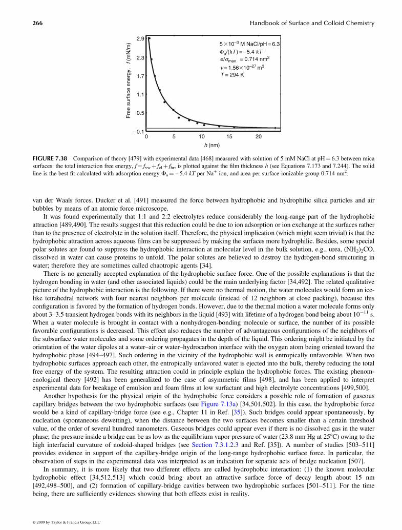
van der Waals forces. Ducker et al. [491] measured the force between hydrophobic and hydrophilic silica particles and airbubbles by means of an atomic force microscope.

It was found experimentally that 1:1 and 2:2 electrolytes reduce considerably the long-range part of the hydrophobicattraction [489,490]. The results suggest that this reduction could be due to ion adsorption or ion exchange at the surfaces ratherthan to the presence of electrolyte in the solution itself. Therefore, the physical implication (which might seem trivial) is that thehydrophobic attraction across aqueous films can be suppressed by making the surfaces more hydrophilic. Besides, some specialpolar solutes are found to suppress the hydrophobic interaction at molecular level in the bulk solution, e.g., urea, (NH2)2CO,dissolved in water can cause proteins to unfold. The polar solutes are believed to destroy the hydrogen-bond structuring inwater; therefore they are sometimes called chaotropic agents [34].

There is no generally accepted explanation of the hydrophobic surface force. One of the possible explanations is that thehydrogen bonding in water (and other associated liquids) could be the main underlying factor [34,492]. The related qualitativepicture of the hydrophobic interaction is the following. If there were no thermal motion, the water molecules would form an ice-like tetrahedral network with four nearest neighbors per molecule (instead of 12 neighbors at close packing), because thisconfiguration is favored by the formation of hydrogen bonds. However, due to the thermal motion a water molecule forms onlyabout 3–3.5 transient hydrogen bonds with its neighbors in the liquid [493] with lifetime of a hydrogen bond being about 10�11 s.When a water molecule is brought in contact with a nonhydrogen-bonding molecule or surface, the number of its possiblefavorable configurations is decreased. This effect also reduces the number of advantageous configurations of the neighbors ofthe subsurface water molecules and some ordering propagates in the depth of the liquid. This ordering might be initiated by theorientation of the water dipoles at a water–air or water–hydrocarbon interface with the oxygen atom being oriented toward thehydrophobic phase [494–497]. Such ordering in the vicinity of the hydrophobic wall is entropically unfavorable. When twohydrophobic surfaces approach each other, the entropically unfavored water is ejected into the bulk, thereby reducing the totalfree energy of the system. The resulting attraction could in principle explain the hydrophobic forces. The existing phenom-enological theory [492] has been generalized to the case of asymmetric films [498], and has been applied to interpretexperimental data for breakage of emulsion and foam films at low surfactant and high electrolyte concentrations [499,500].

Another hypothesis for the physical origin of the hydrophobic force considers a possible role of formation of gaseouscapillary bridges between the two hydrophobic surfaces (see Figure 7.13a) [34,501,502]. In this case, the hydrophobic forcewould be a kind of capillary-bridge force (see e.g., Chapter 11 in Ref. [35]). Such bridges could appear spontaneously, bynucleation (spontaneous dewetting), when the distance between the two surfaces becomes smaller than a certain thresholdvalue, of the order of several hundred nanometers. Gaseous bridges could appear even if there is no dissolved gas in the waterphase; the pressure inside a bridge can be as low as the equilibrium vapor pressure of water (23.8 mm Hg at 258C) owing to thehigh interfacial curvature of nodoid-shaped bridges (see Section 7.3.1.2.3 and Ref. [35]). A number of studies [503–511]provides evidence in support of the capillary-bridge origin of the long-range hydrophobic surface force. In particular, theobservation of steps in the experimental data was interpreted as an indication for separate acts of bridge nucleation [507].

In summary, it is more likely that two different effects are called hydrophobic interaction: (1) the known molecularhydrophobic effect [34,512,513] which could bring about an attractive surface force of decay length about 15 nm[492,498–500], and (2) formation of capillary-bridge cavities between two hydrophobic surfaces [501–511]. For the timebeing, there are sufficiently evidences showing that both effects exist in reality.

0–0.1

0.5

1.1

1.7

2.3

2.95 �10–3 M NaCl/pH = 6.3Φa/(kT ) = –5.4 kTe/smax = 0.714 nm2

n = 1.56�10–27 m3

T = 294 K

5 10

h (nm)

f (

mN

/m)

15 20

FIGURE 7.38 Comparison of theory [479] with experimental data [468] measured with solution of 5 mM NaCl at pH¼ 6.3 between micasurfaces: the total interaction free energy, f¼ fvwþ felþ fhr, is plotted against the film thickness h (see Equations 7.173 and 7.244). The solidline is the best fit calculated with adsorption energy Fa¼�5.4 kT per Naþ ion, and area per surface ionizable group 0.714 nm2.




Fre

e su

rfac

e en

ergy

,

7.4.5.5 Fluctuation Wave Forces

All fluid interfaces, including liquid membranes and surfactant lamellas, are involved in a thermal fluctuation wave motion. Theconfigurational confinement of such thermally exited modes within the narrow space between two approaching interfaces givesrise to short-range repulsive surface forces, which are considered below.

7.4.5.5.1 Undulation ForcesThe undulation force arises from the configurational confinement related to the bending mode of deformation of two fluidbilayers. This mode consists in undulation of the bilayer at constant bilayer area and thickness (Figure 7.39a). Helfrich et al.[514,515] established that two such bilayers, apart at a mean distance h, experience a repulsive disjoining pressure given by theexpression:

Pund(h) ¼ 3p2(kT)2

64kth3(7:247)

where kt is the bending elastic modulus of the bilayer as a whole. The experiment [516] and the theory [35,192] show that kt isof the order of 10�19 J for lipid bilayers. The undulation force has been measured, and the dependence Pund / h�3 confirmedexperimentally [517–519].

7.4.5.5.2 Peristaltic ForceThe peristaltic force [476] originates from the configurational confinement related to the peristaltic (squeezing) mode ofdeformation of a fluid bilayer (Figure 7.39b). This mode of deformation consists in fluctuation of the bilayer thickness at fixedposition of the bilayer midsurface. The peristaltic deformation is accompanied with extension of the bilayer surfaces.Israelachvili and Wennerstöm [476] demonstrated that the peristaltic disjoining pressure is related to the stretching modulus,ks, of the bilayer:

Pper(h) � 2(kT)2

p2ksh5(7:248)

The experiment [520] gives values of ks varying between 135 and 500 mN m�1, depending on temperature and composition ofthe lipid membrane.

h

(c)

h

(b)

h

(a)

FIGURE 7.39 Surface forces due to configurational confinement of thermally exited modes into a narrow region of space betweentwo approaching interfaces: (a) bending mode of membrane fluctuations giving rise to the undulation force; (b) squeezing mode ofmembrane fluctuations producing the peristaltic force; (c) fluctuating protrusion of adsorbed amphiphilic molecules engendering theprotrusion surface force.




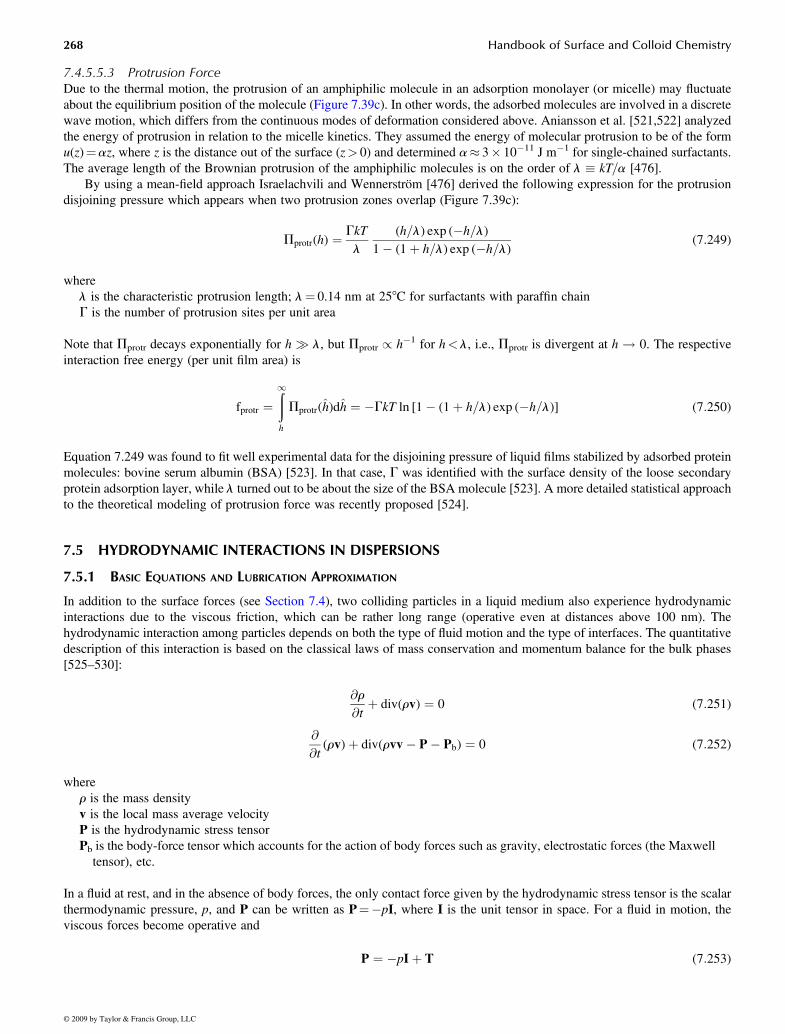
7.4.5.5.3 Protrusion ForceDue to the thermal motion, the protrusion of an amphiphilic molecule in an adsorption monolayer (or micelle) may fluctuateabout the equilibrium position of the molecule (Figure 7.39c). In other words, the adsorbed molecules are involved in a discretewave motion, which differs from the continuous modes of deformation considered above. Aniansson et al. [521,522] analyzedthe energy of protrusion in relation to the micelle kinetics. They assumed the energy of molecular protrusion to be of the formu(z)¼az, where z is the distance out of the surface (z> 0) and determined a� 3� 10�11 J m�1 for single-chained surfactants.The average length of the Brownian protrusion of the amphiphilic molecules is on the order of l � kT=a [476].

By using a mean-field approach Israelachvili and Wennerström [476] derived the following expression for the protrusiondisjoining pressure which appears when two protrusion zones overlap (Figure 7.39c):

Pprotr(h) ¼ GkT

l

(h=l) exp (�h=l)

1� (1þ h=l) exp (�h=l)(7:249)

wherel is the characteristic protrusion length; l¼ 0.14 nm at 258C for surfactants with paraffin chainG is the number of protrusion sites per unit area

Note that Pprotr decays exponentially for h � l, but Pprotr / h�1 for h< l, i.e., Pprotr is divergent at h ! 0. The respectiveinteraction free energy (per unit film area) is

fprotr ¼ð1

h

Pprotr(h)dh ¼ �GkT ln [1� (1þ h=l) exp (�h=l)] (7:250)

Equation 7.249 was found to fit well experimental data for the disjoining pressure of liquid films stabilized by adsorbed proteinmolecules: bovine serum albumin (BSA) [523]. In that case, G was identified with the surface density of the loose secondaryprotein adsorption layer, while l turned out to be about the size of the BSA molecule [523]. A more detailed statistical approachto the theoretical modeling of protrusion force was recently proposed [524].

7.5 HYDRODYNAMIC INTERACTIONS IN DISPERSIONS

7.5.1 BASIC EQUATIONS AND LUBRICATION APPROXIMATION

In addition to the surface forces (see Section 7.4), two colliding particles in a liquid medium also experience hydrodynamicinteractions due to the viscous friction, which can be rather long range (operative even at distances above 100 nm). Thehydrodynamic interaction among particles depends on both the type of fluid motion and the type of interfaces. The quantitativedescription of this interaction is based on the classical laws of mass conservation and momentum balance for the bulk phases[525–530]:

@r

@tþ div(rv) ¼ 0 (7:251)

@

@t(rv)þ div(rvv� P� Pb) ¼ 0 (7:252)

wherer is the mass densityv is the local mass average velocityP is the hydrodynamic stress tensorPb is the body-force tensor which accounts for the action of body forces such as gravity, electrostatic forces (the Maxwelltensor), etc.

In a fluid at rest, and in the absence of body forces, the only contact force given by the hydrodynamic stress tensor is the scalarthermodynamic pressure, p, and P can be written as P¼�pI, where I is the unit tensor in space. For a fluid in motion, theviscous forces become operative and

P ¼ �pIþ T (7:253)




where T is the viscous stress tensor. From the definition of the stress tensor (Equation 7.253), it follows that the resultanthydrodynamic force, F, exerted by the surrounding fluid on the particle surface, S, and the torque, M, applied to it are given bythe expressions [525,527]

F ¼ðS

P n dS, M ¼ðS

r0 � P n dS (7:254)

wherer0 is the position vector of a point of S with respect to an arbitrarily chosen coordinate originn is the vector of the running unit normal to the surface S

In the presence of body forces, the total force, Ftot, and torque, Mtot, acting on the particle surface are

Ftot ¼ FþðS

Pb n dS, Mtot ¼ MþðS

r0 � Pb n dS (7:255)

The dependence of the viscous stress on the velocity gradient in the fluid is a constitutive law, which is usually called the bulkrheological equation. The general linear relation between the viscous stress tensor, T, and the rate of strain tensor,

D ¼ 12[rvþ (rv)T] (7:256)

(the superscript T denotes conjugation) reads

T ¼ z(div v)Iþ 2h D� 13(div v)I

� �(7:257)

The latter equation is usually referred as the Newtonian model or Newton’s law of viscosity. In Equation 7.257, z is thedilatational bulk viscosity and h is the shear bulk viscosity. The usual liquids comply well with the Newtonian model. On theother hand, some concentrated macromolecular solutions, colloidal dispersions, gels, etc., may exhibit non-Newtonianbehavior; their properties are considered in detail in some recent review articles and books [530–533]. From Equations7.252 and 7.257, one obtains the Navier–Stokes equation [534,535]:

rdv

dt¼ �rpþ z þ 1

3h

� �r(r v)þ hr2vþ f , (f � DPb) (7:258)

for homogeneous Newtonian fluids, for which the dilatational and shear viscosities, z and h, do not depend on the spatialcoordinates. In Equation 7.258, the material derivative d=dt can be presented as a sum of a local time derivative and aconvective term:

d

dt¼ @

@tþ (v r) (7:259)

If the density, r, is constant, the equation of mass conservation (Equation 7.251) and the Navier–Stokes Equation 7.258reduce to

div v ¼ 0, rdv

dt¼ �rpþ hr2vþ f (7:260)

For low shear stresses in the dispersions, the characteristic velocity, Vz, of the relative particle motion is small enough in orderfor the Reynolds number, Re¼ rVzL=h, to be a small parameter, where L is a characteristic length scale. In this case, the inertiaterms in Equations 7.258 and 7.260 can be neglected. Then, the system of equations becomes linear and the different types ofhydrodynamic motion become additive [368,536,537]; e.g., the motion in the liquid flow can be presented as a superposition ofelementary translation and rotational motions.

The basic equations can be further simplified in the framework of the lubrication approximation, which can be applied tothe case when the Reynolds number is small and when the distances between the particle surfaces are much smaller than their




radii of curvature (Figure 7.40) [538,539]. There are two ways to take into account the molecular interactions between the twoparticles across the liquid film intervening between them: (1) the body force approach; (2) the disjoining pressure approach. Theformer approach treats the molecular forces as components of the body force, f (Equation 7.258); consequently, they givecontributions to the normal and tangential stress boundary conditions [540,541]. In the case (2), the molecular interactionsare incorporated only in the normal stress boundary conditions at the particle surfaces. When the body force can be expressedas a gradient of potential, f¼rU (that is Pb¼UI), the two approaches are equivalent [542].

If two particles are interacting across an electrolyte solution, the equations of continuity and the momentum balance,Equation 7.260, in lubrication approximation read [543]

rII vII þ @vz@z

¼ 0, h@2vII@z2

¼ rIIpþ kTXNi¼1

zicirIIF,@p

@zþ kT

XNi¼1

zici@F

@z¼ 0 (7:261)

where vII and rII are the projection of the velocity and the gradient operator on the plane xy; the z-axis is (approximately)perpendicular to the film surfaces S1 and S2 (see Figure 7.40); ci¼ ci (r, z, t) is the ion concentration (i¼ 1, 2, . . . , N); F is thedimensionless electric potential (see Sections 7.2.1.2 and 7.2.2). It turns out that in lubrication approximation, the dependenceof the ionic concentrations on the z coordinate comes through the electric potential F (r, z, t): we obtain a counterpart ofthe Boltzmann equation ci ¼ ci,n (r, z, t) exp (�ziF), where ci,n refers to an imaginary situation of switched off electric charges(F � 0). The kinematic boundary condition for the film surfaces has the form:

@hj@t

þ uj rIIhj ¼ (vz)j at Sj(j ¼ 1,2) (7:262)

where ui is the velocity projection in the plane xy at the corresponding film surface, Si, which is close to the interfacialvelocity; (vz)i is the z component of the velocity at the surface Si. The general solution of Equations 7.261 and 7.262 could bewritten as:

p ¼ pn þ kTXNi¼1

(ci � ci,n) (7:263)

vII ¼ (z� h1)(z� h2)

2hrIIpn þ h2 � z

hu1 þ z� h1

hu2

þ kTh2

4h

XNi¼1

m2,i(z)� h2 � z

hm2,i(h1)� z� h1

hm2,i(h2)

� �rIIci,n (7:264)

Here h¼ h2� h1 is the local film thickness; the meaning of pn (x, y, t) is analogous to that of ci,n (x, y, t); the functions, mk,i (z),account for the distribution of the ith ionic species in the EDL:

m0,i � exp (�ziF)� 1, mk,i(z) � 2h

ðz

0

mk�1,i (z)dz (k ¼ 1, 2, 3, i ¼ 1, 2, . . . ,N) (7:265)

Droplet phase

F ilm phase0

z

r

S2: z = h2(t,r)

S1: z = h1(t,r)

FIGURE 7.40 Sketch of a plane-parallel film formed between two identical fluid particles.




The equation determining the local thickness, h, of a film with fluid surfaces (or, alternatively, determining the pressuredistribution at the surfaces of the gap between two solid particles of known shape) is

@h

@tþrII h

2(u1 þ u2)

� �¼ 1

12hrII (h3rIIp) þ kT

8hrII h3

XNi¼1

[m2,i(h1)þ m2,i(h2)� m3,i(h2)þ m3,i(h1)]rIIci,n

" #(7:266)

The problem for the interactions upon central collisions of two axisymmetric particles (bubbles, droplets, or solid spheres) atsmall surface-to-surface distances was first solved by Reynolds [538] and Taylor [544,545] for solid surfaces and by Ivanovet al. [546,547] for films of uneven thickness. Equation 7.266 is referred to as the general equation for films with deformablesurfaces [546,547] (see also the more recent reviews [223,548,549]). The asymptotic analysis [550–552] of the dependence ofthe drag and torque coefficient of a sphere, which is translating and rotating in the neighborhood of a solid plate, is also basedon Equation 7.266 applied to the special case of stationary conditions.

Using Equation 7.255, one can obtain expressions for the components of the total force exerted on the particle surface, S, inthe lubrication approximation:

Ftot,z ¼ðS

pn þ kTXNi¼1

(cis � ci,n)þPnel � p1

" #dS (7:267)

Ftot,II ¼ �ðS

h@vII@z

þ 2kTk2c

@F

@zrIIF

� �dS (7:268)

where p1 is the pressure at infinity in the meniscus region (Figure 7.40) and Pnel � P�Pel accounts for the contribution ofnonelectrostatic (nondouble layer) forces to the disjoining pressure (see Section 7.4). The normal and the lateral forceresultants, Fz and FII, are the hydrodynamic resistance and shear force, respectively.

7.5.2 INTERACTION BETWEEN PARTICLES OF TANGENTIALLY IMMOBILE SURFACES

The surfaces of fluid particles can be treated as tangentially immobile when they are covered by dense surfactant adsorptionmonolayers that can resist tangential stresses [223,548,549,553,554]. In such a case, the bubbles or droplets behave as flexibleballs with immobile surfaces. When the fluid particles are rather small (say, microemulsion droplets), they can behave like hardspheres; therefore, some relations considered below, which were originally derived for solid particles, can be also applied tofluid particles.

7.5.2.1 Taylor and Reynolds Equations, and Influence of the Particle Shape

In the case of two axisymmetric particles moving along the z-axis toward each other with velocity Vz¼�dh=dt Equation 7.266can be integrated, and from Equation 7.267 the resistance force can be calculated. The latter turns out to be proportional to thevelocity and bulk viscosity and depends on the shape in a complex way. For particles with tangentially immobile surfaces andwithout surface electric charge (u1¼ u2¼ 0, F¼ 0) Charles and Mason [555] have derived

Fz ¼ 6phVz

ð1

0

r3

h3dr (7:269)

where r is the radial coordinate in a cylindrical coordinate system. In the case of two particles of different radii, R1 and R2, filmradius R, and uniform film thickness h (see Figure 7.41), from Equation 7.269 the following expression can be derived[556,557]:

Fz ¼ 32phVz

R2*h

1þ R2

hR*þ R4

h2R2*

!, R* � 2R1R2

(R1 þ R2)(7:270)

This geometrical configuration has proved to be very close to the real one in the presence of electrostatic disjoining pressure[239]. The Charles–Mason formula (Equation 7.269) and Equation 7.267 have been used to calculate the velocity of film




thinning for a large number of cases, summarized by Hartland [558] in tables for more than 50 cases (two- and three-dimensional small drops, fully deformed large drops subjected to large forces, two-dimensional hexagonal drops, etc.).

Setting R¼ 0 in Equation 7.270, we can derive a generalized version of the Taylor formula [544,545] for the velocity ofapproach of two nondeformable spheres under the action of an external (nonviscous) force, Fz [557]:

VTa ¼ 2hFz

3phR2*

(7:271)

When a solid sphere of radius Rc approaches a flat solid surface, we may use the Taylor formula with R*¼ 2Rc when the gapbetween the two surfaces is small compared to Rc. In fact Equation 7.271 does not appear in any G.I. Taylor’s publications butin the article by Hardy and Bircumshaw [544] it was published (see Ref. [545]).

In the case when two plane-parallel ellipsoidal discs of tangentially immobile surfaces are moving against each other underthe action of an external force, Ftot,z, from Equations 7.266 and 7.267, we can derive the Reynolds equation [538] for thevelocity of film thinning:

VRe ¼ Fzh3(a2 þ b2)

3pha3b3(7:272)

where a and b are the principal radii of curvature. If there is a contribution of the disjoining pressure, P, the Reynolds equationfor a flat axisymmetrical film (a¼ b¼R) between two fluid particles of capillary pressure Pc can be written in the form [202]:

VRe ¼ 2Fzh3

3phR4¼ 2(Pc �P)h3

3hR2(7:273)

From Equations 7.270 and 7.273 the ratio between the Reynolds velocity and the velocity of film thinning for a given force isobtained. In Figure 7.42, this ratio is plotted as a function of the film thickness, h, divided by inversion thickness, hi ¼ R2=R*[548]. We see that the influence of the viscous friction in the zone encircling the film (this influence is not accounted for inEquation 7.273) decreases the velocity of thinning about three times for the larger distances, whereas for the small distances thisinfluence vanishes. From Equations 7.270 and 7.271, the ratio between the Taylor velocity (corresponding to nondeformablespheres) and the approaching velocity of two deformable particles can be calculated. The dependence of this ratio on thedistance between the particles for different film radii is illustrated in Figure 7.43. We see that an increase of the film radius, R,and a decrease of the distance, h, lead to a decrease in the velocity. The existence of a film between the particles can decreasethe velocity of particle approach, Vz, by several orders of magnitude.

7.5.2.2 Interactions among Nondeformable Particles at Large Distances

The hydrodynamic interaction between members of a group of small particles suspended in a viscous fluid has fundamentalimportance for the development of adequate models for calculating the particle collective diffusion coefficient and the effectiveviscosity of suspension [368,536,554,559,560]. The Stokesian resistance is determined for a number of specific particle shapes

h

R

R1

R2

FIGURE 7.41 Sketch of a film between two nonidentical fluid particles of radii R1 and R2. The film thickness and radius are denoted byh and R.




under the condition that the particles are located so far apart that the hydrodynamic interactions can be ignored [536]. A generaltheory applicable to a single particle of arbitrary shape has been developed by Brenner [561,562]. This method gives thefirst-order correction (with respect to the particle volume fraction) of the viscosity and diffusivity. Matrix relations betweenresistance and velocity for the pure translational and rotational motions of the members of a general multiparticle systeminvolved in a linear shear flow are given by Brenner and O’Neill [563]. In principle, from these relations we can furtherobtain the higher order terms in the series expansion of the viscosity and diffusivity with respect to the powers of the particlevolume fraction.

At present, the only multiparticle system for which exact values of the resistance tensors can be determined is that of twospheres. It turns out that all types of hydrodynamic flows related to the motion of two spherical particles (of radii R1 and R2) canbe expressed as superpositions of the elementary processes depicted in Figure 7.44 [368,527,536,537,564–573].

The first particle moves toward the second immobile particle and rotates around the line of centers (see Figure 7.44a). Thisis an axisymmetric rotation problem (a two-dimensional hydrodynamic problem) which was solved by Jeffery [565]and Stimson and Jeffery [566] for two identical spheres moving with equal velocities along their line of centers. Cooley andO’Neill [567,568] calculated the forces for two nonidentical spheres moving with the same speed in the same direction,

0.0

1.0

1.2

1.4

1.6

1.8

2.0

2.2

2.4

2.6

2.8

3.0

0.1 0.2 0.3 0.4 0.5

h/hi

VR

e/V

z

0.6 0.7 0.8 0.9 1.0

FIGURE 7.42 Plot of VRe=Vz versus h=hi for two fluid particles (Equation 7.270) which are deformed because of the viscous friction in thetransition zone between the film and the bulk phase (see Figure 7.41).

100

10–4 10–3 10–2

101

102

103

104

R/R∗ = 0.012

2

2

2

1.5 2 3 4 5 6 1.5 2 3 4 5 6

R/R∗ = 0.02R/R∗ = 0.05R/R∗ = 0.1

h/R∗

VT

a/V

z

FIGURE 7.43 Plot of VTa=Vz versus h=R* for various values of the dimensionless film radius, R=R*. VTa corresponds to two nondeformed(spherical) particles (Equation 7.271), whereas Vz is the velocity of approach of two deformed particles (Equation 7.270).




or alternatively, moving toward each other. A combination of these results permits evaluation of the total forces and torquesacting on the particles.

The first particle then moves along an axis perpendicular to the center line and rotates around this axis, whereas the secondparticle is immobile; see Figure 7.44b (this is a typical three-dimensional hydrodynamic problem). The contribution of thisasymmetric motion of the spheres to the resistance tensors was determined by Davis [569] and O’Neill and Majumdar [570].

The first particle moves with linear velocity, U1, under the action of an applied external force, F, whereas the secondparticle is subjected to the hydrodynamic disturbances (created by the motion of the first particle) and moves with a linearvelocity, U2 (see Figure 7.44c). As a rule, this is a three-dimensional hydrodynamic problem. For this case, Batchelor [574] andBatchelor and Wen [575] have derived the following expressions for the instantaneous translational velocities of the twoparticles in an otherwise quiescent and unbounded fluid:

U1 ¼ F

6phR1 A11(r)

rr

r2þ B11(r) I� rr

r2

� �h i(7:274)

U2 ¼ F

6ph(R1 þ R2) A12(r)

rr

r2þ B12(r) I� rr

r2

� �h i(7:275)

where r is the vector connecting the particle centers and r¼ jrj. Expressions for the mobility functions Aij and Bij (i, j¼ 1, 2) atlarge values of the dimensionless distance s¼ 2r=(R1þ R2) and comparable particle radii l¼R2=R1¼O(1) have been derivedby Jeffrey and Onishi [576] and Davis and Hill [573]. The derived far-field expansions are

1� B11 ¼ 68l5

(1þ l)6s6þ 32l3(10� 9l2 þ 9l4)

(1þ l)8s8þ 192l5(35� 18l2 þ 6l4)

(1þ l)10s10þ O(s�12)

B11 � A11 ¼ 60l3

(1þ l)4s4� 60l3(8� l2)

(1þ l)6s6þ 32l3(20� 123l2 þ 9l4)

(1þ l)8s8þ 64l2(175þ 1500l� 426l2 þ 18l4)

(1þ l)10s10þ O(s�12)

A11 � 2A12

1þ l¼ 1� 3

(1þ l)sþ 4(1þ l2)

(1þ l)3s3� 60l3

(1þ l)4s4þ 32l3(15� 4l2)

(1þ l)6s6� 2400l3

(1þ l)7s7

� 192l3(5� 22l2 þ 3l4)

(1þ l)8s8þ 1920l3(1þ l2)

(1þ l)9s9� 256l5(70� 375l� 120l2 þ 9l3)

(1þ l)10s10

� 1536l3(10� 151l2 þ 10l4)

(1þ l)11s11þ O(s�12) (7:276)

B11 � 2B12

1þ l¼ 1� 3

2(1þ l)s� 2(1þ l2)

(1þ l)3s3� 68l5

(1þ l)6s6� 32l3(10� 9l2 þ 9l4)

(1þ l)8s8

� 192l5(35� 18l2 þ 6l4)

(1þ l)10s10� 16l3(560� 553l2 þ 560l4)

(1þ l)11s11þ O(s�12)

F

v

v

(a) (b) (c)

w

w

r

U1

U2

O1

O2 O1

O1

O2O2

R2 R2

R1

R2

R1

R1

FIGURE 7.44 Types of hydrodynamic interactions between two spherical particles: (a) motion along and rotation around the line of centers;(b) motion along and rotation around an axis perpendicular to the line of centers; (c) the first particle moves under the action of an appliedexternal force, F, whereas the second particle is subjected to the hydrodynamic disturbance created by the motion of the first particle.




In the case of a small heavy sphere falling through a suspension of large particles (fixed in space), we have l� 1; the respectiveexpansions, corresponding to Equation 7.276, were obtained by Fuentes et al. [577]. In the opposite case, when l � 1, thesuspension of small background spheres will reduce the mean velocity of a large heavy particle (as compared with its Stokesvelocity [578]) because the suspension behaves as an effective fluid of larger viscosity as predicted by the Einstein viscosityformula [574,577].

7.5.2.3 Stages of Thinning of a Liquid Film

Experimental and theoretical investigations [221,229,548,549,554,579,580] show that during the approach of two fluidcolloidal particles, a flat liquid film can appear between their closest regions (see Figure 7.32). The hydrodynamic interactionsas well as the buoyancy, the Brownian, electrostatic, van der Waals, and steric forces and other interactions can be involved infilm formation [193,239,556,581,582]. The formation and the evolution of a foam or emulsion film usually follows the stagesshown in Figure 7.45.

Under the action of an outer driving force, the fluid particles approach each other. The hydrodynamic interaction isstronger at the front zones and leads to a weak deformation of the interfaces in this front region. In this case, the usualhydrodynamic capillary number, Ca¼hVz=s, which is a small parameter for nondeformable surfaces, should be modified toread Ca¼hVzR*=sh, where the distance, h, between the interfaces is taken into account. The shape of the gap between twodrops for different characteristic times was calculated numerically by many authors [582–602]. Experimental investigation ofthese effects for symmetric and asymmetric drainage of foam films were carried out by Joye et al. [591,592]. In some specialcases, the deformation of the fluid particle can be very fast: for example, the bursting of a small air bubble at an air–waterinterface is accompanied by a complex motion resulting in the production of a high-speed liquid jet (see Boulton-Stone andBlake [602]).

When a certain small separation, hi, the inversion thickness, is reached, the sign of the curvature in the contact of the fluidparticles (drops, bubbles) changes. A concave lens-shaped formation called a dimple is formed (see Frankel and Mysels [603]).This stage is also observed for asymmetric films [592]. A number of theoretical studies have described the development of adimple at the initial stage of film thinning [582–602]. The inversion thickness can be calculated from a simple equation inwhich the van der Waals interaction is explicitly taken into account (see Section 7.4.2) [223,547,582]

hi ¼ Fz(s1 þ s2)

4ps1s21� AHR*

12Fzhi

� �(7:277)

where s1 and s2 are the interfacial tensions of the phase boundaries S1 and S2; in this case Fz is the external force (ofnonviscous and non-van der Waals origin) experienced by the approaching particles; AH is the Hamaker constant. In the case,

Z

0

(a) (b) (c)

(f)(e)(d)

S2

S1

h(r )

z (r )

2Rd

2Rsp

2R

qh2

2RNBF

2R

hr

FIGURE 7.45 Main stages of formation and evolution of a thin liquid film between two bubbles or drops: (a) mutual approach of slightlydeformed surfaces; (b) at a given separation, the curvature at the center inverts its sign and a dimple arises; (c) the dimple disappears, andeventually an almost plane-parallel film forms; (d) due to thermal fluctuations or other disturbances the film either ruptures or transforms into athinner Newton black film (e), which expands until reaching the final equilibrium state (f).




when the van der Waals force is negligible, Equation 7.277 reduces to hi¼Fz(s1þs2)=(4ps1s2) [223,547]. Danov et al. [556]have shown that in the case of Brownian flocculation of identical small droplets, hi obeys the following transcendental equation:

hi ¼ kT

2pszi

ðzi0

ziz

� �2g(z)

g(zi)exp

U(z)� U(zi)

kT

� �dz

zi

8<:

9=;

�1

(7:278)

wherekT is the thermal energy; g(z)¼Fz=Vz is the hydrodynamic resistance given by Equation 7.270U is the potential energy due to the surface forces (see Equation 7.175)z is the distance between the droplet mass centers

These authors pointed out that with an increase of droplet size the role of the Brownian force in the film formation decreases,but for micrometer-sized liquid droplets the Brownian force is still by several orders of magnitude greater than the buoyancyforce due to gravity. If the driving force is large enough, so that it is able to overcome the energy barrier created by theelectrostatic repulsion and=or the increase of the surface area during the droplet deformation, then film with a dimple will beformed. On the contrary, at low electrolyte concentration (i.e., strong electrostatic repulsion) such a dimple might not appear.Parallel experiments [604] on the formation and thinning of emulsion films of macroscopic and microscopic areas, prepared inthe Scheludko cell [202] and in a miniaturized cell, show that the patterns and the time scales of the film evolution in these twocases are significantly different. There is no dimple formation in the case of thin liquid films of small diameters [604].

In the case of predominant van der Waals attraction, instead of a dimple, a reverse bell-shape deformation, called a pimple,appears and the film quickly ruptures [582,589,598,601]. The thickness, hp, at which the pimple appears can be calculated fromthe relationship [582]:

hp ¼AHR*12Fz

� �1=2

(7:279)

The pimple formation thickness depends significantly on the radius, R*. If a drop of tangentially immobile surfaces and radiusRd is driven by the buoyancy force, then we have:

Fz ¼ 43pR3

dDrg (7:280)

whereDr is the density differenceg is the gravity acceleration

For the collision of this drop with another immobile one, we have h2p ¼ AH=(16pDrgR2d). We see that hp is inversely proportional

to the drop radius. For typical values of the Hamaker constant AH¼ 4� 10�20 J, density difference Dr¼ 0.12 g cm�3, andRd¼ 10 mm, the thickness of pimple formation is hp¼ 82.3 nm. Note that this thickness is quite large. The pimple formation canbe interpreted as the onset of instability without fluctuations (stability analysis of the film intervening between the drops hasbeen carried out elsewhere [60]).

As already mentioned, if the van der Waals force (or other attractive force) is not predominant, first a dimple forms in thethinning liquid films. Usually the dimple exists for a short period of time; initially it grows, but as a result of the swift outflow ofliquid it decreases and eventually disappears. The resulting plane-parallel film thins at almost constant radius R. When theelectrostatic repulsion is strong, a thicker primary film forms (see point 1 in Figure 7.17). From the viewpoint of conventionalDLVO theory, this film must be metastable. Indeed, the experiments with microscopic foam films, stabilized with sodium octylsulfate or SDS in the presence of different amount of electrolyte [605], show that a black spot may suddenly form and atransition to secondary (Newton black) film may occur (see point 2 in Figure 7.17). The rate of thinning depends not only on thecapillary pressure (the driving force) but also very strongly on the surfactant concentration (for details, see Section 7.5.3.2).

The appearance of a secondary film (or film rupture, if the secondary film is not stable) is preceded by corrugation of thefilm surfaces due to thermally excited fluctuations or outer disturbances. When the derivative of the disjoining pressure, @P=@h,is positive, the amplitude of the fluctuations (z in Figure 7.45d) spontaneously grows. As already mentioned, the instabilityleads to rupture of the film or to formation of black spots. The theory of film stability was developed by de Vries [606], Vrij[607], Felderhof [540], Sche and Fijnaut [541], Ivanov et al. [608], Gumerman and Homsy [609], Malhotra and Wasan [610],




Maldarelli and Jain [542], and Valkovska et al. [611]. On the basis of the lubrication approximation for tangentially immobilesurfaces, Ivanov et al. [608] and Valkovska et al. [611] derived a general expression for the critical film thickness, hcr, by usinglong-waves stability analysis:

hcr ¼ htrsh2trkT

� �1=4

exp � k2crR2

32h3cr

ðhtrhcr

h3P0

Pc �Pdh

0B@

1CA (7:281)

where kcr is the wave number of the critical wave defined as

k2cr ¼

1s

ðhtrhcr

h3P0

Pc �Pdh

ðhtrhcr

h6

Pc �Pdh

(7:282)

In Equation 7.282, htr is the so-called transitional thickness [607,608,611] at which the increase of free energy due to theincreased film area and the decrease of free energy due to the van der Waals interaction in the thinner part (Figure 7.45d)compensate each other. At htr the most rapidly growing fluctuation (the critical wave) becomes unstable. The transitionalthickness obeys the following equation [608,611]:

24h3cr[Pc �P(htr)]

R2k2crh4tr

þ sk2crh3tr

2h3cr¼ P0(htr) (7:283)

Figures 7.46 and 7.47 show the critical thicknesses of rupture, hcr, for foam and emulsion films, respectively, plotted versus thefilm radius [612]. In both cases the film phase is the aqueous phase, which contains 4.3� 10�4 M SDSþ added NaCl. Theemulsion film is formed between two toluene drops. Curve 1 is the prediction of a simpler theory, which identifies the criticalthickness with the transitional one [610]. Curve 2 is the theoretical prediction of Equations 7.281 through 7.283 (no adjustableparameters); in Equation 7.182 for the Hamaker constant the electromagnetic retardation effect has also been taken into account[368]. In addition, Figure 7.48 shows the experimental dependence of the critical thickness versus the concentration ofsurfactant (dodecanol) for aniline films. Figures 7.46 through 7.48 demonstrate that when the film area increases and=or theelectrolyte concentration decreases the critical film thickness becomes larger. Figure 7.49 show the critical thickness of foamfilm rupture for three concentrations of SDS in the presence of 0.3 M NaCl [500]. The dashed and dash-dotted lines, for 1 and10 mM SDS, respectively, are computed assuming only the van der Waals attraction (no adjustable parameter). The deviation of

FIGURE 7.46 Dependence of the critical thickness, hcr, on the radius, R, of foam films. The experimental points are data from Ref. [612];the films are formed from a solution of 4.3� 10�4 M SDSþ 0.25 M NaCl. Curve 1 is the prediction of the simplified theory [610], whereasCurve 2 is calculated using Equations 7.281 through 7.283; no adjustable parameters.




100 200 300

Film radius (µm)

(2)

(1)

400 500 600020

30

40

50

Film

thic

knes

s (n

m)

60

70

the predicted values of hcr from the measured is because of the hydrophobic interaction (Section 7.4.5.4.2). The solid linesrepresent fits with the decay length of the hydrophobic interactions l0¼ 15.8 nm using Equations 7.281 through 7.283.

The surface corrugations do not necessarily lead to film rupture. Instead, black spots (secondary films of very low thickness;h2 in Figure 7.17) can be formed. The typical thickness of plane-parallel films at stage c (Figure 7.45c) is about 200 nm, whilethe characteristic thickness h2 of the Newton black film (Figures 7.45e and f) is about 5–10 nm. The black spots either coalesceor grow in diameter, forming an equilibrium secondary (Newton black) film with a thickness h2 and radius Rsp. These spotsgrow until they cover the whole film area.

After the entire film area is occupied by the Newton black film, the film radius increases until it reaches its equilibriumvalue, R¼RNBF (Figure 7.45f). Finally, the equilibrium contact angle is established. For more details about this last stage offilm thinning, see part IV.C of Ref. [223].

7.5.2.4 Dependence of Emulsion Stability on the Droplet Size

Experimental data [614,615] show that the emulsion stability correlates well with the lifetime of separate thin emulsion films orof drops coalescing with their homophase. To simplify the treatment we will consider here the lifetime of a single drop pressedagainst its homophase under the action of gravity. To define the lifetime (or drainage time) t, we assume that in the initial andfinal moments the film has some known thicknesses hin and hf:

FIGURE 7.47 Critical thickness, hcr, versus radius, R, of emulsion films, toluene=water=toluene. The experimental points are data fromRef. [612]; the films are formed from a solution of 4.3� 10�4 M SDSþ 0.1 M NaCl. Curve 1 is the prediction of the simplified theory [610],whereas Curve 2 is calculated using Equations 7.281 through 7.283; no adjustable parameters.

FIGURE 7.48 Dependence of the critical thickness, hcr, of aniline films on the concentration of dodecanol, c0. (Modified from Ivanov, I.B.,Pure Appl. Chem., 52, 1241, 1980. With permission.)




020

25

30

35

40

45

Film

thic

knes

s (n

m)

50

55

100 200 300

Film radius (µm)

400 500

(1)

(2)

10–110–2

Surfactant concentration, c0 (M)

Crit

ical

thic

knes

s, h

cr (

Å)

300

400

500

10–3

t ¼ðhinhf

dh

Vz

¼ 3phR2*

2Fz

lnhinhf

� �þ R2

hfR*1� hf

hin

� �þ R4

2h2fR2*

1� h2fh2in

� �" #(7:284)

The final thickness, hf, may coincide with the critical thickness of film rupture. Equation 7.284 is derived for tangentiallyimmobile interfaces from Equation 7.270 at a fixed driving force (no disjoining pressure).

In the case of gravity-driven coalescence of a droplet with its homophase, the driving force is given by Equation 7.280 andthe mean drop radius is R*¼ 2Rd. Then from Equations 7.280 and 7.284 we can deduce the droplet lifetime in the so-calledTaylor regime, corresponding to nondeformed droplets (R¼ 0):

tTa ¼ 6phR2d

Fz

lnhinhf

� �¼ 9h

2gRdDrln

hinhf

� �(7:285)

We see that tTa depends logarithmically on the ratio of the initial and final thickness. Moreover, in the Taylor regime thelifetime, t, decreases with the increase of the driving force, Fz, and the drop radius, Rd. The latter fact is confirmed by theexperimental data of Dickinson et al. [616].

In the case of deformed drops (R 6¼ 0), the drainage time, t, is determined by Equation 7.284, and in such a case the fluidparticles approach each other in the Reynolds regime [548,613]. The dependence of t on Rd in Equation 7.284 is very complex,because the driving force, Fz, and the film radius, R, depend on Rd. The film radius can be estimated from the balance of thedriving and capillary force [548,613]:

R2 ¼ FzRd

2ps(7:286)

In this regime, the lifetime, t, increases with an increase of the driving force, Fz. This is exactly the opposite trend compared toresults for the Taylor regime (see Equation 7.285). The result can be rationalized in view of Reynolds equation (Equation7.273). In the numerator of this equation, Fz / R3

d, whereas in the denominator R4 / R8d (see Equation 7.286); as a result, the

drainage rate becomes proportional to R�5d , i.e., Vz decreases as the droplet radius increases.

The numerical results from Equations 7.284 through 7.286 for the lifetime or drainage time, t, versus the droplet radius, Rd,are plotted in Figure 7.50 for parameter values typical for emulsion systems: Dr¼ 0.2 g cm�3, h¼ 1 cP, hf¼ 5 nm, andhin¼Rd=10. The various curves in Figure 7.50 correspond to different values of the surface tension, s, shown in the figure. Theleft branches of the curves correspond to the Taylor regime (nondeformed droplets), whereas the right branches correspond tothe Reynolds regime (formation of film between the droplets). The presence of a deep minimum on the t versus Rd curve wasfirst pointed out by Ivanov [617,618]. The theoretical dependencies in Figure 7.50 agree well with experimental data [619–621]for the lifetime of oil droplets pressed by the buoyancy force against a large oil–water interface in a system containing proteinBSA (Figure 7.51).

FIGURE 7.49 Critical thickness, hcr, versus the film radius at a 0.3 M fixed concentration of NaCl for three SDS concentrations: 0.5, 1, and10 mM. The dashed and dash-dotted lines, for 1 and 10 mM SDS, respectively, are computed using an absence of the hydrophobic attraction.The solid lines are fits of the experimental points with l0¼ 15.8 nm.




100 120

Film radius (µm)

Added 0.3 M NaCI

14060

25

30

35

Crit

ical

thic

knes

s (n

m)

401.0 µM SDS (without Πhb)

10.0 µM SDS (without Πhb)

0.5 µM SDS1.0 µM SDS

10.0 µM SDS

80

7.5.3 EFFECT OF SURFACE MOBILITY

The hydrodynamic interactions between fluid particles (drops, bubbles) suspended in a liquid medium depend on the interfacialmobility. In the presence of surfactants, the bulk fluid motion near an interface disturbs the homogeneity of the surfactantadsorption monolayer. The ensuing surface-tension gradients act to restore the homogeneous equilibrium state of themonolayer. The resulting transfer of adsorbed surfactant molecules from the regions of lower surface tension toward theregions of higher surface tension constitutes the Marangoni effect. The analogous effect, for which the surface-tension gradientis caused by a temperature gradient, is known as the Marangoni effect of thermocapillarity. In addition, the interfaces possessspecific surface rheological properties (surface elasticity and dilatational and shear surface viscosities), which give rise to theso-called Boussinesq effect (see below) [622].

00

1

2

3

4

5

6

s = 1 dyn/cm s = 3 dyn/cm s = 10 dyn/cm

s = 30 dyn/cm

7

20 40

Life

time,

t

(s)

60 80 100 120

Droplet radius, Rd (µm)

140

Taylor

160 180 200

FIGURE 7.50 Calculated lifetime, t, of drops approaching a fluid interface in Taylor regime (the solid line) and in Reynolds regime(the other lines) as a function of the droplet radius, Rd.

Droplet radius (µm)

Taylorregime

Reynoldsregime

Dro

plet

life

time

(s)

6000

0

20

40

60

80

100

120

140

160

100 200 300 400 500 700 800 900 1000 1100

FIGURE 7.51 Stability of oil drops pressed by buoyancy against a large oil=water interface. Measured lifetime, (the points), is plottedversus droplet radius in a system consisting of soybean oil and aqueous solution of 410�4 wt% BSAþ 0.15 M NaCl (pH¼ 6.4). The solidline is drawn in accordance to Equation 7.284.




7.5.3.1 Diffusive and Convective Fluxes at an Interface—Marangoni Effect

To take into account the influence of surfactant adsorption, Equations 7.251 and 7.252 are to be complemented with transportequations for each of the species (k¼ 1,2, . . . , N) in the bulk phases [525,528,553,554]

@ck@t

þ div(ckvþ jk) ¼ rk (k ¼ 1, 2, . . . ,N) (7:287)

where ck and jk are bulk concentration and flux, respectively, of the kth species—note that jk includes the molecular diffusiveflux, the flux driven by external forces (e.g., electrodiffusion [543,553,554]) and the thermodiffusion flux [553]; and rk is therate of production due to chemical reactions, including surfactant micellization or micelle decay. The surface mass-balanceequation for the adsorption, Gk, has the form [543,553,554]:

@Gk

@tþrs (Gkvs þ jsk) ¼ rsk þ n < jk> (7:288)

wheren is the unit normal to the interface directed from phase 1 to 2<> denotes the difference between the values of a given physical quantity at the two sides of the interfacers is the surface gradient operator [623]vs is the local material surface velocityjsk is the two-dimensional flux of the kth component along the interfacersk accounts for the rate of production of the kth component due to interfacial chemical reactions and could include

conformational changes of adsorbed proteins

Equation 7.288 provides a boundary condition for the normally resolved flux, jk. From another viewpoint, Equation 7.288represents a two-dimensional analog of Equation 7.287. The interfacial flux, jsk, can also contain contributions from theinterfacial molecular diffusion, electrodiffusion, and thermodiffusion. A simple derivation of the time-dependent convective-diffusion equation for surfactant transport along a deforming interface is given by Brenner and Leal [624–627], Davis et al.[560], and Stone [628]. If the molecules are charged, the bulk and surfaces electrodiffusion fluxes can be expressed in the form[543,629,630]:

jk ¼ �Dk(rck þ zkckrF), jsk ¼ �Dsk(rsGk þ zkGkrsF) (7:289)

for the bulk and interfacial phase. Here, Dk and Dsk are the bulk and surface collective diffusion coefficients, respectively, which

are connected with the diffusion coefficients of individual molecules, Dk,0 and Dsk,0, through the relationship [630]

Dk ¼ Dk,0

kT

Kb(fk)

(1� fk)

@mk

@ lnfk, Ds

k ¼Ds

k,0

kTKs(Gk)

@msk

@ lnGk(7:290)

where mk and msk are the bulk and surface chemical potentials, respectively. The dimensionless bulk friction coefficient, Kb,

accounts for the change in the hydrodynamic friction between the fluid and the particles (created by the hydrodynamicinteractions between the particles). The dimensionless surface mobility coefficient, Ks, accounts for the variation of the frictionof a molecule in the adsorption layer. Feng [631] has determined the surface diffusion coefficient, the dilatational elasticity, andthe viscosity of a surfactant adsorption layer by theoretical analysis of experimental data. Stebe and Maldarelli [632,633]studied theoretically the surface diffusion driven by large adsorption gradients. The determination of bulk and surface diffusioncoefficients from experimental data for the drainage of nitrobenzene films stabilized by different concentrations of dodecanolwas reported [629].

Note that the adsorption isotherms, relating the surface concentration, Gk, with the subsurface value of the bulk concen-tration, ck (see Section 7.2.2.1), or the respective kinetic Equation 7.86 for adsorption under barrier control (see Section7.2.2.5), should also be employed in the computations based on Equations 7.287 through 7.290 for a complete set of equationsto be obtained.

Another boundary condition is the equation of the interfacial momentum balance [529,548,554]:

rs s ¼ n <Pþ Pb> (7:291)




where s is the interfacial stress tensor, which is a two-dimensional counterpart of the bulk stress tensor, P. Moreover, a two-dimensional analog of Equations 7.253, 7.256, and 7.257, called the Boussinesq–Scriven constitutive law, can be postulated fora fluid interface [223,554,622,634–638]:

s ¼ saIs þ (hdl � hsh)(rs vs)Is þ hsh (rs vs)Is þ Is(rs vs)T� �

(7:292)

wherehdl and hsh are the interfacial dilatational and shear viscosities, respectivelyIs is the unit surface idemfactor [623]sa is the scalar adsorption part of the surface tension (see Section 7.2.1.2.2)

In view of the term saIs in Equation 7.292, the Marangoni effects are hidden in the left-hand side of the boundary condition(Equation 7.291) through the surface gradient of sa:

rssa ¼ �XNk¼1

Ek

GkrsGk � ET

TrsT , Ek ¼ � @sa

@ lnGk

� �T,Gj 6¼k

, ET ¼ � @sa

@ ln T

� �Gk

(7:293)

whereEk is the Gibbs elasticity for the kth surfactant species (see Equation 7.6)ET represents the thermal analog of the Gibbs elasticity

The thermocapillary migration of liquid drops or bubbles and the influence of ET on their motion are investigated in a number ofworks [639–641].

In fact, Equation 7.292 describes an interface as a two-dimensional Newtonian fluid. On the other hand, a number of non-Newtonian interfacial rheological models have been described in the literature [642–645]. Tambe and Sharma [646] modeledthe hydrodynamics of thin liquid films bounded by viscoelastic interfaces, which obey a generalized Maxwell model for theinterfacial stress tensor. These authors [647,648] also presented a constitutive equation to describe the rheological properties offluid interfaces containing colloidal particles. A new constitutive equation for the total stress was proposed by Horozov et al.[649], Danov et al. [650], and Ivanov et al. [651] who applied a local approach to the interfacial dilatation of adsorption layers.

When the temperature is not constant, the bulk heat transfer equation complements the system and involves Equations7.251, 7.252, and 7.287. The heat transfer equation is a special case of the energy balance equation. It should be noted that morethan 20 various forms of the overall differential energy balance for multicomponent systems are available in the literature[525,528]. The corresponding boundary condition can be obtained as an interfacial energy balance [554,638]. Based on thederivation of the bulk [652] and interfacial [650,653] entropy inequalities (using the Onsager theory), various constitutiveequations for the thermodynamic mass, heat, and stress fluxes have been obtained.

7.5.3.2 Fluid Particles and Films of Tangentially Mobile Surfaces

When the surface of an emulsion droplet is mobile, it can transmit the motion of the outer fluid to the fluid within the droplet.This leads to a special pattern of the fluid flow and affects the dissipation of energy in the system. The problem concerning theapproach of two nondeformed (spherical) drops or bubbles of pure phases has been investigated by many authors[548,576,577,583,584,654–659]. A number of solutions, generalizing the Taylor equation (Equation 7.271), have beenobtained. For example, the velocity of central approach, Vz, of two spherical drops in pure liquid is related to the hydrodynamicresistance force, Fz, by means of a Padé-type expression derived by Davis et al. [583]

Vz ¼ 2hFz

3phR2*

1þ 1:711j þ 0:461j2

1þ 0:402j, j ¼ h

hd

ffiffiffiffiffiffiR*2h

r(7:294)

whereh is the closest surface-to-surface distance between the two dropshd is the viscosity of the disperse phase (the liquid in the droplets)

In the limiting case of solid particles, we have hd ! 1, and Equation 7.294 reduces to the Taylor equation (Equation 7.271).Note that in the case of close approach of two drops (j� 1), the velocity Vz is proportional to

ffiffiffih

p. This implies that the two

drops can come into contact (h¼ 0) in a finite period of time (t<1) under the action of a given force, Fz, because the integral




in Equation 7.284 is convergent for hf¼ 0. This is in contrast to the case of immobile interfaces (j � 1), when Vz / h andt ! 1 for hf ! 0.

In the other limiting case, that of two nondeformed gas bubbles (hd ! 0) in pure liquid, Equation 7.294 cannot be used;instead, Vz can be calculated from the expression due to Beshkov et al. [659]

Vz ¼ Fz

2phRd ln (Rd=h)(7:295)

Note that in this case Vz / (ln h)�1, and the integral in Equation 7.284 is convergent for hf ! 0. In other words, the theorypredicts that the lifetime, t, of a doublet of two colliding spherical bubbles in pure liquid is finite. Of course, the real lifetime ofa doublet of bubbles or drops is affected by the surface forces for h< 100 nm, which should be accounted for in Fz and whichmay lead to the formation of thin film in the zone of contact [193,356].

Let us proceed with the case of deformed fluid particles (Figure 7.32). A number of theoretical studies [660–663] have beendevoted to the thinning of plane-parallel liquid films of pure liquid phases (no surfactant additives). Ivanov and Traykov [662]derived the following exact expressions for the velocity of thinning of an emulsion film:

Vz ¼ 32DP2

rdhdR4

� �1=3

h5=3,Vz

VRe¼ 1

«e, «e � rdhdh

4Fz

108ph3R4

� �1=3

(7:296)

whererd is the density of the disperse phaseVRe is the Reynolds velocity defined by Equation 7.273«e is the so-called emulsion parameter

Substituting typical parameter values in Equations 7.294 and 7.296, we can check that at a given constant force the velocity ofthinning of an emulsion film is smaller than the velocity of approach of two nondeformed droplets and much larger than VRe. Itis interesting to note that the velocity of thinning as predicted by Equation 7.296 does not depend on the viscosity of thecontinuous phase, h, and its dependence on the drop viscosity, hd, is rather weak. There are experimental observationsconfirming this prediction (see Ref. [32], p. 381).

The presence of surfactant adsorption monolayers decreases the mobility of the droplet (bubble) surfaces. This is due to theMarangoni effect (see Equation 7.293). From a general viewpoint, we may expect that the interfacial mobility will decreasewith the increase of surfactant concentration until eventually the interfaces become immobile at high surfactant concentrations(see Section 7.5.2); therefore, a pronounced effect of surfactant concentration on the velocity of film drainage should beexpected. This effect really exists (see Equation 7.297), but in the case of emulsions it is present only when the surfactant ispredominantly soluble in the continuous phase.

Traykov and Ivanov [663] established (both theoretically and experimentally) the interesting effect that when the surfactantis dissolved in the disperse phase (that is, in the emulsion droplets), the droplets approach each other just as in the case of pureliquid phases, i.e., Equation 7.296 holds. Qualitatively, this effect can be attributed to the fact that the convection-drivensurface-tension gradients are rapidly damped by the influx of surfactant from the drop interior; in this way, the Marangoni effectis suppressed. Indeed, during the film drainage the surfactant is carried away toward the film border, and a nonequilibriumdistribution depicted in Figure 7.52a appears. Because, however, the mass transport is proportional to the perturbation, thelarger the deviation from equilibrium, the stronger the flux tending to eliminate the perturbation (the surfactant flux is denotedby thick arrows in Figure 7.52b). In this way, any surface concentration gradient (and the related Marangoni effect) disappears.The emulsion films in this case behave as if surfactant is absent.

(a) (b)

FIGURE 7.52 Damping of convection-driven surface-tension gradients by influx of surfactant from the drop interior. (a) Since the masstransport is proportional to the perturbation, the larger the perturbation, the stronger the flux tending to eliminate it. (b) Uniform surfactantdistribution is finally reached.




In the opposite case, when the surfactant is soluble in the continuous phase, the Marangoni effect becomes operative andthe rate of film thinning becomes dependent on the surface (Gibbs) elasticity (see Equation 7.293). Moreover, the convection-driven local depletion of the surfactant monolayers in the central area of the film surfaces gives rise to fluxes of bulk and surfacediffusion of surfactant molecules. The exact solution of the problem [543,546,579,629,630,663] gives the following expressionfor the rate of thinning of symmetrical planar films (of both foam and emulsion type):

Vz

VRe¼ 1þ 1

«e þ «f,

1«f

¼ 6hDs

hEG

þ 3hDG(@s=@c)

(7:297)

whereD and Ds are the bulk and interfacial collective diffusion coefficients (see Equation 7.290)EG is the Gibbs elasticity«f is the so-called foam parameter [613]

In the special case of foam film, one substitutes «e¼ 0 in Equation 7.297. Note that the diffusive surfactant transport, whichtends to restore the uniform adsorption monolayers, damps the surface-tension gradients (which oppose the film drainage) andthus accelerates the film thinning. However, at large surfactant concentrations, the surface elasticity, EG, prevails, «f increases,and, consequently, the thinning rate decreases down to the Reynolds velocity, Vz ! VRe (see Equation 7.297). Similarexpressions for the rate of film thinning, which are appropriate for various ranges of values of the interfacial parameters,can be found in the literature [223,547,548,594,664,665]. A table describing the typical ranges of variation of theinterfacial properties (G, EG, D, Ds, @s=@c, etc.) for emulsion and foam systems can be found in Ref. [223], Table 7.2therein. For h< 100 nm, the influence of the disjoining pressure should be taken into account (see Equation 7.273). In somestudies [223,557,646,666–669], the effect of the interfacial viscosity on the rate of thinning and the lifetime of plane-parallelfilms is investigated; this effect is found to decrease when the film thickness, h, becomes smaller and the film radius, R,becomes larger.

Note that Equation 7.297 does not hold in the limiting case of foam films («e¼ 0) at low surfactant concentration, «f ! 0.The following expression is available for this special case [613]:

Vz=VRe ¼ (1þ 1=«f )=[1þ 4h2=(3R2«f )] (7:298)

The merit of Equation 7.298 is that it gives as limiting cases both Vz=VRe for foam films without surfactant, «f ! 0, andEquation 7.297 with «e¼ 0 (note that in the framework of the lubrication approximation, used to derive Equation 7.297, theterms / h2=R2 are being neglected). Equation 7.298 has also some shortcomings, which are discussed in Ref. [613].

Another case, which is not described by Equations 7.297 and 7.298, is the approach of two nondeformed (spherical)bubbles in the presence of surfactant. The velocity of approach in this case can be described by means of the expression[547,557,618,630]:

Vz

VTa

¼ hszh

h(1þ b)

hsþ 1

� �Ln

hsh(1þ b)

þ 1

� �� 1

� �1

(7:299)

where the parameters b and hs account for the influence of bulk and surface diffusivity of surfactants, respectively. FromEquation 7.290 these parameters are calculated to be [630]

b � 3hcD0Kb(f)

kTG2(1� f), hs � 6hDs

0Ks(G)

kTG(7:300)

Generalization of Equation 7.299 to the more complicated case of two nondeformed (spherical) emulsion droplets with accountfor the influence of surface viscosity has been published in Ref. [557].

Returning to the parameter values, we note that usually «e � «f and «e � 1. Then, comparing the expressions for Vz=VRe asgiven by Equations 7.296 and 7.297, we conclude that the rate of thinning is much greater when the surfactant is dissolved inthe droplets (the disperse phase) in comparison with the case when the surfactant is dissolved in the continuous phase. Thisprediction of the theory was verified experimentally by measuring the number of films that rupture during a given period of time[670], as well as the rate of thinning. When the surfactant was dissolved in the drop phase, the average lifetime was the same forall surfactant concentrations (Figure 7.53a), in agreement with Equation 7.296. For the emulsion film with the same, but




inverted, liquid phases (the former continuous phase becomes disperse phase, and vice versa), i.e., the surfactant is in the filmphase, the average lifetime is about 70 times longer—compare curves in Figure 7.53a with curve B in Figure 7.53b.The theoretical conclusions have been also checked and proved in experimental measurements with nitroethane dropletsdispersed in an aqueous solution of the cationic surfactant hexadecyl trimethyl ammonium chloride (HTAC) [615].

7.5.3.3 Bancroft Rule for Emulsions

There have been numerous attempts to formulate simple rules connecting the emulsion stability with the surfactant properties.Historically, the first one was the Bancroft rule [671], which states that ‘‘to have a stable emulsion the surfactant must besoluble in the continuous phase.’’ A more sophisticated criterion was proposed by Griffin [672] who introduced the conceptof hydrophilic–lipophilic balance (HLB). As far as emulsification is concerned, surfactants with an HLB number in therange of 3–6 must form water in oil (W=O) emulsions, whereas those with HLB numbers from 8 to 18 are expected toform O=W emulsions. Different formulae for calculating the HLB numbers are available; for example, the Davies expression[673] reads

HLB ¼ 7þ (hydrophilic group number) � 0:475nc (7:301)

where nc is the number of –CH2– groups in the lipophilic part of the molecule. Schinoda and Friberg [674] proved that the HLBnumber is not only a property of the surfactant molecules, but also depends strongly on the temperature (for nonionicsurfactants), on the type and concentration of added electrolytes, on the type of oil phase, etc. They proposed using thephase inversion temperature (PIT) instead of HLB for characterization of the emulsion stability.

Davis [675] summarized the concepts of HLB, PIT, and Windsor’s ternary phase diagrams for the case of microemulsionsand reported topological ordered models connected with the Helfrich membrane bending energy. Because the curvature ofsurfactant lamellas plays a major role in determining the patterns of phase behavior in microemulsions, it is important to revealhow the optimal microemulsion state is affected by the surface forces determining the curvature energy [222,676,677]. It ishoped that lattice models [678,679] and membrane curvature models [680,681] will lead to predictive formulae for themicroemulsion design.

Ivanov et al. [613,617,618,682] have proposed a semiquantitative theoretical approach that provides a straightforwardexplanation of the Bancroft rule for emulsions. This approach is based on the ideas of Davies and Rideal [32] that both types ofemulsions are formed during the homogenization process, but only the one with lower coalescence rate survives. If the initialdrop concentration for both emulsions is the same, the coalescence rates for the two emulsions—(Rate)1 for emulsion 1 and(Rate)2 for emulsion 2 (Figure 7.54)—will be proportional to the respective coalescence rate constants, kc,1 and kc,2 (see Section7.6), and inversely proportional to the film lifetimes, t1 and t2:

(Rate)1(Rate)2

� kc,1kc,2

� t2t1

� V1

V2(7:302)

0 5 10

2 mM0.1 mM0 mM

t (s)(a)

15 200.0

0.5

1.0

1.5∆N

I(N

∆t)

(s–1

)

2.0

00.00

0.05

0.10

0.15

∆N/(

N∆t

) (s

–1)

0.20

0.25AB

10 20t (s)(b)

30 40 50

FIGURE 7.53 Histograms for the lifetimes of emulsion films: DN=N is the relative number of films that have ruptured during a time intervalDt. (a) Surfactant in the drops: benzene films between water drops containing surfactant sodium octylsulfonate of concentration: 0 M, 0.1 mM,and 2 mM; (b) Surfactant in the film: (a) benzene film with 0.1 M of lauryl alcohol dissolved in the film, (b) water film with 2 mM of sodiumoctylsulfonate inside [670].




where V1 and V2 denote the respective velocities of film thinning. After some estimates based on Equations 7.273, 7.284, 7.296,and 7.297, we can express the ratio in Equation 7.302 in the form:

(Rate)1(Rate)2

� (486rdD3s )

1=3 h3cr,1h2cr,2

!1=3hd

R2

� �1=3 Pc �P1

EG(Pc �P2)2=3

(7:303)

where hcr,1 and hcr,2 denote the critical thickness of film rupture for the two emulsions in Figure 7.54. Many conclusions can bedrawn, regarding the type of emulsion to be formed:

1. If the disjoining pressures, P1 and P2, are zero, the ratio in Equation 7.303 will be very small. Hence, emulsion 1(surfactant soluble in the continuous phase) will coalesce much more slowly and it will survive. This underlines thecrucial importance of the surfactant location (which is connected with its solubility), thus providing a theoreticalfoundation for Bancroft’s rule. The emulsion behavior in this case will be controlled almost entirely by thehydrodynamic factors (kinetic stability).

2. Disjoining pressure, P, plays an important role. It can substantially change and even reverse the behavior of thesystem if it is comparable by magnitude with the capillary pressure, Pc. For example, if (Pc�P2)! 0 at a finite valueof Pc�P1 (which may happen, for example, for an O=W emulsion with oil soluble surfactant), the ratio in Equation7.303 may become much larger than unity, which means that emulsion 2 will become thermodynamically stable. Insome cases the stabilizing disjoining pressure is large enough for emulsions with a very high volume fraction of thedisperse phase (above 95% in some cases) to be formed [683].

3. Gibbs elasticity, EG, favors the formation of emulsion 1, because it slows down the film thinning. On the other hand,increased surface diffusivity, Ds, decreases this effect, because it helps the interfacial tension gradients to relax, thusfacilitating the formation of emulsion 2.

4. Film radius, R, increases and capillary pressure, Pc, decreases with the drop radius, Rd. Therefore, larger drops willtend to form emulsion 1, although the effect is not very pronounced.

5. Difference in critical thicknesses of the two emulsions only slightly affects the rate ratio in Equation 7.303, althoughthe value of hcr itself is important.

6. Viscosity of the continuous phase, h, has no effect on the rate ratio, which depends only slightly on the viscosity of thedrop phase, hd. This is in agreement with the experimental observations [32].

7. Interfacial tension, s, affects the rate ratio directly only through the capillary pressure, Pc¼ 2s=Rd. The electrolyteprimarily affects the electrostatic disjoining pressure, P, which decreases as the salt content increases, thus destabil-izing the O=W emulsion. It can also influence the stability by changing the surfactant adsorption (including the case ofnonionic surfactants).

8. Temperature strongly affects the solubility and surface activity of nonionic surfactants [3]. It is well known that athigher temperature nonionic surfactants become more oil soluble, which favors the W=O emulsion. Thus, solubilitymay change the type of emulsion formed at the PIT. The surface activity has numerous implications, the mostimportant is the change of the Gibbs elasticity, EG, and the interfacial tension, s.

Emulsion 1 Emulsion 2

Phase II

Phase I

Phase I

Phase II

FIGURE 7.54 The two possible types of emulsions obtained just after the homogenization; the surfactant is soluble into phase I.




9. Surface-active additives (cosurfactants, demulsifiers, etc.), such as fatty alcohols in the case of ionic surfactants, mayaffect the emulsifier partitioning between the phases and its adsorption, thereby changing the Gibbs elasticity and theinterfacial tension. The surface-active additive may also change the surface charge (mainly by increasing the spacingamong the emulsifier ionic headgroups), thus decreasing the repulsive electrostatic disjoining pressure and favoringthe W=O emulsion. Polymeric surfactants and adsorbed proteins increase the steric repulsion between the filmsurfaces. They may favor either O=W or W=O emulsions, depending on their conformation at the interface andtheir surface activity.

10. Interfacial bending moment, B0, can also affect the type of the emulsion, although this is not directly visible fromEquation 7.303. (Note that B0¼�4kcH0, where H0 is the so-called spontaneous curvature and kc is the interfacialcurvature elastic modulus [188]. Typically, B0 is of the order of 5�10�11 N.) Usually, for O=W emulsions, B0 opposesthe flattening of the droplet surfaces in the zone of collision (Figure 7.32), but for W=O emulsions it favors flattening[193]. This effect might be quantified by the expression for the curvature contribution in the energy of droplet–dropletinteraction [193]:

Wc ¼ �2pR2B0=Rd, (R=Rd)2 � 1 (7:304)

It turns out thatWc> 0 for the droplet collisions in an O=Wemulsion, whileWc< 0 for aW=O emulsion [193]. Consequently, theinterfacial bending moment stabilizes the O=W emulsions but destabilizes the W=O ones. There is supporting experimentalevidence [684] for microemulsions, i.e., for droplets of rather small size. Moreover, the effect of the bending moment can beimportant even for micrometer-sized droplets [193]. This is because the bent area increases faster (R2 / Rd

2) than the bendingenergy per unit area decreases (Wc=R

2 / 1=Rd) when the droplet radius, Rd, increases (see Equation 7.304).For micron-sized emulsion droplets the capillary pressure can be so high that a film may not appear between the drops. In

such case, instead of Equation 7.303, we can use analogous expression for nondeformed (spherical) drops [685].

7.5.3.4 Demulsification

It has been known for a long time [32] that one way to destroy an emulsion is to add a surfactant, which is soluble in the dropphase—this method is termed chemical demulsification. To understand the underlying process, let us consider two collidingemulsion droplets with film formed in the zone of collision (see Figures 7.32 and 7.55). As discussed above, when the liquid isflowing out of the film, the viscous drag exerted on the film surfaces (from the side of the film interior) carries away theadsorbed emulsifier toward the film periphery. Thus, a nonuniform surface distribution of the emulsifier (shown in Figure 7.55aby empty circles) is established. If demulsifier (the closed circles in Figure 7.55b) is present in the drop phase, it will occupy theinterfacial area freed by the emulsifier. The result will be saturation of the adsorption layer, as shown in Figure 7.55b. If thedemulsifier is sufficiently surface active, its molecules will be able to decrease substantially, and even to eliminate completely,the interfacial tension gradients, thus changing the emulsion to type 2 (see Figure 7.54 and Section 7.5.3.2). This leads to a

(a)

(b)

FIGURE 7.55 (a) Nonuniform surface distribution of an emulsifier due to drag from the draining film. (b) Suppression of the surface-tensiongradients by a demulsifier added in the drop phase.




strong increase in the rate of film thinning, rapid drop coalescence, and emulsion destruction [617,618]. The above mechanismsuggests that the demulsifier has to possess the following properties:

1. Soluble in the drop phase or in both phases, but in the latter case its solubility in the drop phase must be much higher.2. Diffusivity and concentration must be large enough to provide a sufficiently large demulsifier flux toward the surfaces

and thus eliminate the gradients of the interfacial tension.3. Surface activity must be comparable and even higher than that of the emulsifier; otherwise, even though it may adsorb,

it will not be able to suppress the interfacial tension gradients.

In regard to defoaming, various mechanisms are possible, which are discussed in Section 7.7.

7.5.4 INTERACTIONS IN NONPREEQUILIBRATED EMULSIONS

The common nonionic surfactants are often soluble in both water and oil phases. In the practice of emulsion preparation, thesurfactant (the emulsifier) is initially dissolved in one of the liquid phases and then the emulsion is prepared by homogenization.In such a case, the initial distribution of the surfactant between the two phases of the emulsion is not in equilibrium; therefore,surfactant diffusion fluxes appear across the surfaces of the emulsion droplets. The process of surfactant redistribution usuallylasts from several hours to days, until finally equilibrium distribution is established. The diffusion fluxes across the interfaces,directed either from the continuous phase toward the droplets or the reverse, are found to stabilize both thin films andemulsions. In particular, even films, which are thermodynamically unstable, may exist several days because of the diffusionsurfactant transfer; however, they rupture immediately after the diffusive equilibrium has been established. Experimentally, thiseffect manifests itself in phenomena called cyclic dimpling [686] and osmotic swelling [687]. These two phenomena, as well asthe equilibration of two phases across a film [688,689], are described and interpreted below.

7.5.4.1 Surfactant Transfer from Continuous to Disperse Phase (Cyclic Dimpling)

The phenomenon of cyclic dimpling was first observed [618,686] with xylene films intervening between two water droplets inthe presence of the nonionic emulsifier Tween 20 or Tween 80 (initially dissolved in water but also soluble in oil). The samephenomenon also has been observed with other emulsion systems.

After the formation of such an emulsion film, it thins down to an equilibrium thickness (approximately 100 nm),determined by the electrostatic repulsion between the interfaces. As soon as the film reaches this thickness, a dimplespontaneously forms in the film center and starts growing (Figure 7.56a). When the dimple becomes bigger and approachesthe film periphery, a channel forms connecting the dimple with the aqueous phase outside the film (Figure 7.56b). Then, thewater contained in the dimple flows out leaving an almost plane-parallel film behind. Just afterward, a new dimple starts togrow and the process repeats again. The period of this cyclic dimpling remains approximately constant for many cycles andcould be from a couple of minutes up to more than 10 min. It was established that this process is driven by the depletion of the

(a)(b)

inside the film bythe moving surfaces

Surfactant diffusiontoward oil phase

Surfactant diffusiontoward oil phase

Movement ofthe surfaces due to

the Marangoni effect

Surfactant concentrationinside the film is depleted

Decreased surfactantadsorption because of

dissolving in the oil

FIGURE 7.56 Spontaneous cyclic dimpling caused by surfactant diffusion from the aqueous film toward the two adjacent oil phases.(a) Schematic presentation of the process. (b) Photograph of a large dimple just before flowing out; the interference fringes in reflected lightallow determination of the dimple shape.




Liquid being drawn

surfactant concentration on the film surfaces due to the dissolving of surfactant in the adjacent drop phases. The depletiontriggers a surface convection flux along the two film surfaces and a bulk diffusion flux in the film interior. Both fluxes aredirected toward the center of the film. The surface convection causes a tangential movement of the film surfaces; the latter dragalong a convective influx of solution in the film, which feeds the dimple. Thus, the cyclic dimpling appears to be a processleading to stabilization of the emulsion films and emulsions due to the influx of additional liquid in the region between thedroplets, which prevents them from a closer approach, and eventually, from coalescence.

Combining the general equation of films with deformable interfaces (Equation 7.266), the mass balance (Equations 7.287and 7.288), and the boundary condition for the interfacial stresses (Equation 7.292), we can derive [690]:

@h

@tþ 13hr

@

@rrh3

@

@r

s

r

@

@rr@h

@r

� �þP(h)

� �� ¼ 1

2r@

@r

jhr2

G

� �(7:305)

wherej is the diffusion flux in the drop phaser is the radial coordinateh(r, t) is the film thicknesss is the surface tensionG is the adsorptionP is the disjoining pressure

The comparison between the numerical calculations based on Equation 7.305 and the experimental data for the cyclic dimplingwith the anionic surfactant sodium nonylphenol polyoxyethylene-25 sulfate shows a very good agreement (Figure 7.57). Theexperimental points are obtained from the interference fringes (see Figure 7.56). The shape in the initial moment, t¼ 0, servesas an initial condition for determining h(r, t) by solving Equation 7.305. The curves for t¼ 3, 9, 17, and 29 s representtheoretical predictions. The scaling parameters along the h and r axes in Figure 7.57 are h0¼ 350 nm and R¼ 320 mm, with thelatter the film radius; the only adjustable parameter is the diffusion flux, j.

7.5.4.2 Surfactant Transfer from Disperse to Continuous Phase (Osmotic Swelling)

Velev et al. [615] reported that emulsion films, formed from preequilibrated phases containing the nonionic surfactant Tweenand 0.1 M NaCl, spontaneously thin to Newton black films (thickness� 10 nm) and then rupture. However, when the nonionicsurfactant Tween 20 or Tween 60 is initially dissolved in the xylene drops and the film is formed from the nonpreequilibratedphases, no black film formation and rupture are observed [618,687]. Instead, the films have a thickness above 100 nm, and weobserve formation of channels of larger thickness connecting the film periphery with the film center (Figure 7.58). We mayobserve that the liquid is circulating along the channels for a period from several hours to several days. The phenomenoncontinues until the redistribution of the surfactant between the phases is accomplished. This phenomenon occurs only when thebackground surfactant concentration in the continuous (the aqueous) phase is not lower than the CMC. These observations canbe interpreted in the following way.

0.00

1

2

3

4

5

6

7

8

9

0.2 0.4 0.6r/R

h/h

0

0.8

Initial3 s9 s17 s29 s

1.0

FIGURE 7.57 Comparison between the theory of cyclic dimpling (the lines) and the experimental data (the points) for the dimple shape,h(r), determined from the interference fringes (see Figure 7.56b); emulsifier is anionic surfactant sodium nonylphenol polyoxyethylene-25sulfate and the oil phase is styrene.




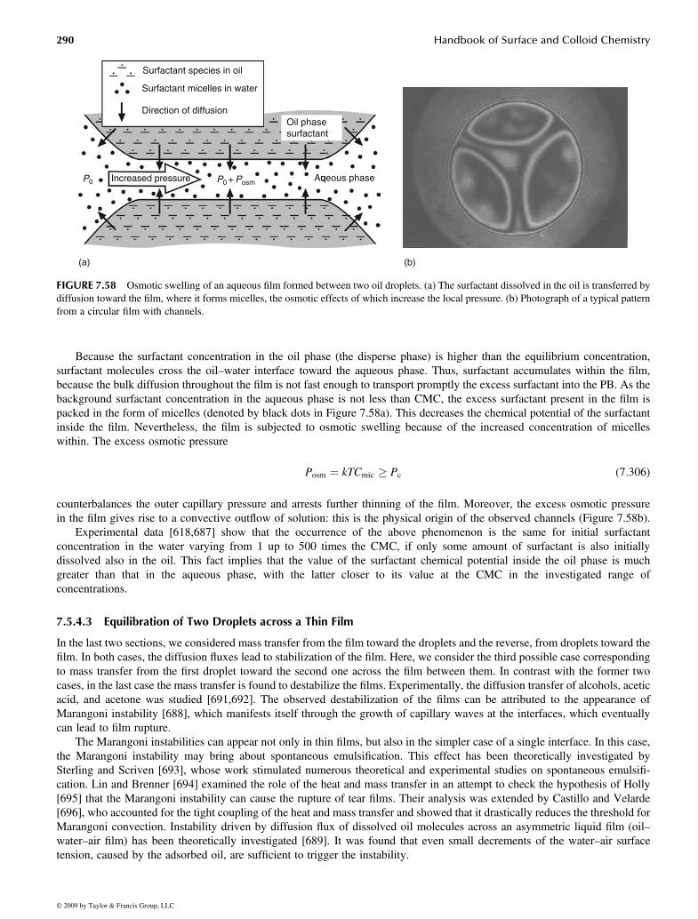
Because the surfactant concentration in the oil phase (the disperse phase) is higher than the equilibrium concentration,surfactant molecules cross the oil–water interface toward the aqueous phase. Thus, surfactant accumulates within the film,because the bulk diffusion throughout the film is not fast enough to transport promptly the excess surfactant into the PB. As thebackground surfactant concentration in the aqueous phase is not less than CMC, the excess surfactant present in the film ispacked in the form of micelles (denoted by black dots in Figure 7.58a). This decreases the chemical potential of the surfactantinside the film. Nevertheless, the film is subjected to osmotic swelling because of the increased concentration of micelleswithin. The excess osmotic pressure

Posm ¼ kTCmic � Pc (7:306)

counterbalances the outer capillary pressure and arrests further thinning of the film. Moreover, the excess osmotic pressurein the film gives rise to a convective outflow of solution: this is the physical origin of the observed channels (Figure 7.58b).

Experimental data [618,687] show that the occurrence of the above phenomenon is the same for initial surfactantconcentration in the water varying from 1 up to 500 times the CMC, if only some amount of surfactant is also initiallydissolved also in the oil. This fact implies that the value of the surfactant chemical potential inside the oil phase is muchgreater than that in the aqueous phase, with the latter closer to its value at the CMC in the investigated range ofconcentrations.

7.5.4.3 Equilibration of Two Droplets across a Thin Film

In the last two sections, we considered mass transfer from the film toward the droplets and the reverse, from droplets toward thefilm. In both cases, the diffusion fluxes lead to stabilization of the film. Here, we consider the third possible case correspondingto mass transfer from the first droplet toward the second one across the film between them. In contrast with the former twocases, in the last case the mass transfer is found to destabilize the films. Experimentally, the diffusion transfer of alcohols, aceticacid, and acetone was studied [691,692]. The observed destabilization of the films can be attributed to the appearance ofMarangoni instability [688], which manifests itself through the growth of capillary waves at the interfaces, which eventuallycan lead to film rupture.

The Marangoni instabilities can appear not only in thin films, but also in the simpler case of a single interface. In this case,the Marangoni instability may bring about spontaneous emulsification. This effect has been theoretically investigated bySterling and Scriven [693], whose work stimulated numerous theoretical and experimental studies on spontaneous emulsifi-cation. Lin and Brenner [694] examined the role of the heat and mass transfer in an attempt to check the hypothesis of Holly[695] that the Marangoni instability can cause the rupture of tear films. Their analysis was extended by Castillo and Velarde[696], who accounted for the tight coupling of the heat and mass transfer and showed that it drastically reduces the threshold forMarangoni convection. Instability driven by diffusion flux of dissolved oil molecules across an asymmetric liquid film (oil–water–air film) has been theoretically investigated [689]. It was found that even small decrements of the water–air surfacetension, caused by the adsorbed oil, are sufficient to trigger the instability.

Oil phasesurfactant

Aqueous phaseIncreased pressure

(a) (b)

P0 P0 + Posm

Surfactant species in oil

Surfactant micelles in water

Direction of diffusion

FIGURE 7.58 Osmotic swelling of an aqueous film formed between two oil droplets. (a) The surfactant dissolved in the oil is transferred bydiffusion toward the film, where it forms micelles, the osmotic effects of which increase the local pressure. (b) Photograph of a typical patternfrom a circular film with channels.




7.5.5 HYDRODYNAMIC INTERACTION OF A PARTICLE WITH AN INTERFACE

There are various cases of particle–interface interactions, which require separate theoretical treatment. The simpler case is thehydrodynamic interaction of a solid particle with a solid interface. Other cases are the interactions of fluid particles (oftangentially mobile or immobile interfaces) with a solid surface; in these cases, the hydrodynamic interaction is accompaniedby deformation of the particle. On the other hand, the colloidal particles (both solid and fluid) may hydrodynamically interactwith a fluid interface, which thereby undergoes a deformation. In the case of fluid interfaces, the effects of surfactant adsorption,surface diffusivity, and viscosity affect the hydrodynamic interactions. A special class of problems concerns particles attachedto an interface, which are moving throughout the interface. Another class of problems is related to the case when colloidalparticles are confined in a restricted space within a narrow cylindrical channel or between two parallel interfaces (solid andfluid); in the fluid case, the particles interact simultaneously with both film surfaces.

The theoretical contributions are limited to the case of low Reynolds number [536,537,613,697–699] (mostly for creepingflows, see Section 7.5.1), avoiding the difficulties arising from the nonlinearity of the equations governing the fluid motion athigher velocities. Indeed, for low Reynolds numbers, the term vrv in the Navier–Stokes equation (see Equations 7.258through 7.260) is negligible, and we may apply the method of superposition to solve the resulting linear set of equations. Thismeans that we may first solve the simpler problems about the particle elementary motions: (1) particle translation (withoutrotation) in an otherwise immobile liquid, (2) particle rotation (without translation) in an otherwise immobile liquid, and (3)streamlining of an immobile particle by a Couette or Poiseuille flow. Once the problems about the elementary motions havebeen solved, we may obtain the linear and angular velocity of the real particle motion combining the elementary flows. Theprinciple of combination is based on the fact that for low Reynolds numbers the particle acceleration is negligible, and the netforce and torque exerted on the particle must be zero. In other words, the hydrodynamic drag forces and torques originatingfrom the particle translation and rotation are counterbalanced by those originating from the streamlining:

Ftranslation þ Frotation þ Fstreamlining ¼ 0, Mtranslation þMrotation þMstreamlining ¼ 0 (7:307)

That is the reason why we will now consider expressions for F and M for various types of elementary motions.

7.5.5.1 Particle of Immobile Surface Interacting with a Solid Wall

The force and torque exerted on a solid particle were obtained in the form of a power series with respect to Rd=l, where Rd is theparticle radius and l is the distance from the center of the particle to the wall. Lorentz [700] derived an asymptotic expression forthe motion of a sphere along the normal to a planar wall with an accuracy of up to Rd=l. Faxen [701] developed the method ofreflection for a sphere moving between two parallel planes in a viscous fluid. Using this method, Wakiya [702] considered thecases of motion in flow of Couette and Poiseuille; however, the method employed by him, cannot be applied to small distancesto the wall [559]. The next important step was taken by Dean and O’Neil [703] and O’Neil [704], who found an exact solutionfor the force and the torque acting on a spherical particle moving tangentially to a planar wall at an arbitrary distance from thewall. The limiting case of small distances between the particle and the wall was examined by several authors [550–552,705].Instead of an exact solution of the problem, the authors derived asymptotic formulae for the force and torque. Keh and Tseng[706] presented a combined analytical–numerical study for the slow motion of an arbitrary axisymmetric body along its axis ofrevolution, with the latter normal to a planar surface. The inertial migration of a small solid sphere in a Poiseuille flow wascalculated by Schonberg and Hinch [707] for the case when the Reynolds number for the channel is of the order of unity.

Below, we present expressions for the forces and torques for some of the elementary motions. In all cases we assume thatthe Reynolds number is small, the coordinate plane xy is parallel to the planar wall and h is the shortest surface-to-surfacedistance from the particle to the wall.

First, we consider the case of a pure translational motion: a solid spherical particle of radius Rd that translates alongthe y-axis with a linear velocity U and angular velocity v � 0 in an otherwise quiescent fluid. In spite of the fact that the particledoes not rotate, it experiences a torque, M, directed along the x-axis, due to friction with the viscous fluid. The respectiveasymptotic expressions [550–552] for the components of the drag force, F, and torque, M, read

Fx ¼ 0, Fy ¼ �6phURdfy, Mx ¼ �8phUR2dmx, My ¼ 0 (7:308)

fy ¼ 815

þ 16375

h

Rd

� �ln

2Rd

h

� �þ 0:58461þ O

h

Rd

� �(7:309)

mx ¼ 110

þ 43250

h

Rd

� �ln

2Rd

h

� �� 0:26227þ O

h

Rd

� �(7:310)

where fy and mx are dimensionless drag force and torque coefficients, respectively.




Second, we consider the case of pure rotation: a solid spherical particle of radius Rd is situated at a surface-to-surfacedistance, h, from a planar wall and rotates with angular velocity, v, around the x-axis in an otherwise quiescent fluid. Thecorresponding force and torque resultants are [550–552]

Fx ¼ 0, Fy ¼ �6phvR2d fy, Mx ¼ �8phvR3

dmx, My ¼ 0 (7:311)

fy ¼ 215

lnRd

h

� �� 0:2526 þ O

h

Rd

� �, mx ¼ 2

5ln

Rd

h

� �þ 0:3817þ O

h

Rd

� �(7:312)

From Equations 7.308 through 7.312, it follows that the force and the torque depend weakly (logarithmically) on the distance,h, as compared to the Taylor or Reynolds laws (Equations 7.271 and 7.272).

As discussed in Sections 7.5.2.1 and 7.5.3.2, a fluid particle in the presence of high surfactant concentration can be treatedas a deformable particle of tangentially immobile surfaces. Such a particle deforms when pressed against a solid wall (see theinset in Figure 7.59). To describe the drag due to the film intervening between the deformed particle and the wall, we may usethe expression derived by Reynolds [538] for the drag force exerted on a planar solid ellipsoidal disc, which is parallel to a solidwall and is moving along the y-axis at a distance h from the wall:

Fx ¼ 0, Fy ¼ �phUh

ab(7:313)

Here, a and b are the semiaxes of the ellipse; for a circular disc (or film), we have a¼ b¼R. By combining Equations 7.308 and7.309 with Equation 7.313, we can derive an expression for the net drag force experienced by the deformed particle (the inset inFigure 7.59) when it moves along the y-axis with a linear velocity U:

Fy ¼ �6phURdfy, fy ¼ R2

6hRd

þ 815

þ 16375

h

Rd

� �ln

2Rd

h

� �þ 0:58461þ O

h

Rd

� �(7:314)

whereh and R denote film thickness and radiusRd is the curvature radius of the spherical part of the particle surface

The dependence of the dimensionless drag coefficient, fy, on the distance h for different values of the ratio R=Rd is illustrated inFigure 7.59. The increase of R=Rd and the decrease of h=Rd may lead to an increase of the drag force, fy, by an order ofmagnitude. The reason why the film between a deformed particle and a wall can be responsible for the major part of the energydissipation. Moreover, the formation of doublets and flocks of droplets separated by liquid films seems to be of majorimportance for the rheological behavior of emulsions.

10–6

102

765

765

4

3

2

2 3 4 6 8 2 3 4 6 8

Dim

ensi

onle

ss d

rag

coef

ficie

nt, f

y

101

R/Rd = 0.03

R/Rd = 0.01

h/Rd

R

U

yz

h

R/Rd = 0.00

10–5 10–5

FIGURE 7.59 Deformed fluid particle (the inset) moving tangentially to an immobile solid surface: plot of the dimensionless dragcoefficient, fy, versus the dimensionless film thickness, h=Rd, for three values of the dimensionless film radius, R=Rd (see Equation 7.314).




7.5.5.2 Fluid Particles of Mobile Surfaces

Let us start with the case of pure phases, when surfactant is missing and the fluid–liquid interfaces are mobile. Under theseconditions, the interaction of an emulsion droplet with a planar solid wall was investigated by Ryskin and Leal [708], andnumerical solutions were obtained. A new formulation of the same problem was proposed by Liron and Barta [709]. The caseof a small droplet moving in the restricted space between two parallel solid surfaces was solved by Shapira and Haber[710,711]. These authors used the Lorentz reflection method to obtain analytical solutions for the drag force and the shape of asmall droplet moving in Couette flow or with constant translational velocity.

The more complicated case, corresponding to a viscous fluid particle approaching the boundary between two pure fluidphases (all interfaces deformable), was investigated by Yang and Leal [712,713] who succeeded in obtaining analytical results.

Next, we proceed with the case when surfactant is present and the Marangoni effect becomes operative. Classicalexperiments carried out by Lebedev [714] and Silvey [715] show that the measured velocity of sedimentation, U, of smallfluid droplets in a viscous liquid (pure liquid phases assumed) does not obey the Hadamar [716] and Rybczynski [717]equation:

F ¼ 2phURd

3hd þ 2hhd þ h

(7:315)

where F is the drag force. The limiting case hd ! 0 corresponds to bubbles, whereas in the other limit, hd ! 1, Equation7.315 describes solid particles. Note that Equation 7.315 is derived for the motion of a spherical fluid particle (drop or bubble)of viscosity hd in a liquid of viscosity h in the absence of any surfactant. The explanation of the contradiction between theoryand experiment [714,715] turned out to be very simple: even liquids that are pure from the viewpoint of the spectral analysismay contain some surface-active impurities, whose bulk concentration might be vanishingly low, but which can provide adense adsorption layer at the restricted area of the fluid particle surface. Then, the effects of Gibbs elasticity and interfacialviscosity substantially affect the drag coefficient of the fluid particle. The role of the latter two effects was investigated byLevich [553], Edwards et al. [554], and He et al. [718] for the motion of an emulsion droplet covered with a monolayer ofnonsoluble surfactant (adsorption and=or desorption not present). These authors used the Boussinesq–Scriven constitutive lawof a viscous fluid interface (Equation 7.292), and established that only the dilatational interfacial viscosity, hdl, but not the shearinterfacial viscosity, hsh, influences the drag force. If the surfactant is soluble in both phases and the process of adsorption isdiffusion controlled (see Section 7.2.2.1) the generalization of Equation 7.315 is

F ¼ 2phURd 3� 1þ hd

hþ 2hdl

hRd

þ RdEG

3hDs

2

2þ 2RdD

haDs

þ RdDd

hd,aDs

0BB@

1CCA

�12664

3775 (7:316)

whereDd is the surfactant diffusion coefficient in the drop phasec and cd are the concentrations of surfactant in the continuous and drop phases, respectivelyha¼ @G=@c and hd,a¼ @G=@cd are the slopes of adsorption isotherms with respect to the surfactant concentration

In the limiting case without surfactant Equation 7.316 is reduced to the Hadamar [716] and Rybczynski [717] equation(Equation 7.315).

Danov et al. [313,719–722] investigated theoretically the hydrodynamic interaction of a fluid particle with a fluid interfacein the presence of surfactant. The numerical results of these authors reveal that there is a strong influence of both shear anddilatational interfacial viscosities on the motion of the fluid particle when the particle–interface distance, h, is approximatelyequal to or smaller than the particle radius, Rd. For example, in the presence of an external force acting parallel to the interface(along the y-axis), the stationary motion of the spherical particle close to the viscous interface is a superposition of a translationalong the y-axis with velocity Vy and a rotation (around the x-axis) with an angular velocity, vx (see the inset in Figure 7.50a).The numerical results of Danov et al. [721,722] for Vy and vx normalized by the Stokes velocity, VStokes¼F=(6phRd), areplotted in Figures 7.60a and b versus h=Rd for four different types of interfaces: (1) solid particle and solid wall (see Equations7.308 through 7.310); (2) fluid particle and fluid interface for K¼E¼ 100; (3) the same system as (2) but for K¼E¼ 10;(4) the same system as (2) but for K¼E¼ 1, where

K � hdl=(hRd), E � hsh=(hRd) (7:317)




(For the definition of the interfacial viscosities, hdl and hsh, see Equation 7.292). As seen in Figure 7.60a, the velocity of thesphere, Vy, is less than VStokes for the solid (1) and the highly viscous (2) interfaces, and Vy noticeably decreases when thedistance h decreases. However, in case (4), corresponding to low surface viscosities, the effect is quite different: Vy=VStokes isgreater than unity (the sphere moves faster near the interface than in the bulk), and its dependence on h is rather weak. Theresult about the angular velocity, vx, is also intriguing (Figure 7.60b). The stationary rotation of a sphere close to a solid (1) orhighly viscous (2) interface is in positive direction, i.e., vx> 0. For the intermediate interfacial viscosity (3), the spherepractically does not rotate, whereas, for the interfaces of low viscosity (4), the drop rotates in the opposite direction, i.e., vx< 0.The inversion of the sign of vx is due to the fact that the friction of the particle with the bulk fluid below it (see the inset inFigure 7.60a) becomes stronger than the friction with the interface above the particle.

Finally, we consider the case of a solid particle attached to a liquid–fluid interface. This configuration is depicted in Figure7.21e; note that the position of the particle along the normal to the interface is determined by the value of the three-phasecontact angle. Stoos and Leal [723] investigated the case when such an attached particle is subjected to a flow directed normallyto the interface. These authors determined the critical capillary number, beyond which the captured particle is removed from theinterface by the flow.

Danov et al. [313] examined the case of an attached particle moving along a liquid–gas interface under the action of anapplied force directed tangentially to the interface. The effect of the contact angle (the depth of immersion), as well as the effectof adsorbed surfactant on the drag force, was investigated. These authors also calculated the surface diffusion coefficient of aBrownian particle attached to the liquid surface. Let Dp and Dp0 be the particle surface diffusion coefficient in the presence andin the absence of surfactant, respectively. In Figure 7.61a, we plot the results for Dp=Dp0 versus the solid–liquid–gas contactangle, u, for three different values of the parameters K and E characterizing the surface viscosities (see Equation 7.317):

FIGURE 7.60 Spherical particle moving tangentially to a viscous interface: plots of the stationary dimensionless linear (Vy=VStokes) (a) andangular (vxRd=VStokes) (b) velocities versus the dimensionless thickness, h=Rd. The curves correspond to various surface viscosities: (1)K¼E¼1 (solid surfaces); (2) K¼E¼ 100; (3) K¼E¼ 10, and (4) K¼E¼ 1 (see Equation 7.317).




0.001–0.10

–0.08

–0.06

(4)

(4)

(3)

(3)

(2)

(2)

(1)

(1)

–0.04

–0.02

wxR

d/V

Sto

kes

Vy/V

Sto

kes

0.00

0.02

0.04

0.2

0.001

(a)

(b)

0.251 0.501

h/Rd

h/Rd

zy

h

Vy

Rd

w x

0.751 1.001

0.3

0.4

0.5

0.6

0.7

0.8

0.9

1.0

1.1

1.2

0.251 0.501 0.751 1.001

(1) K¼E¼ 1; (2) K¼E¼ 5, and (3) K¼E¼ 10. The relatively small slope of the curves in Figure 7.61a indicates that Dp=Dp0

depends less significantly on the contact angle, u, than on the surface viscosity characterized by K and E. Note, however, thatDp0 itself depends markedly on u: the absolute value of Dp0 is smaller for the smaller values of u (for deeper immersion of theparticle in the liquid phase). Figure 7.61b presents the calculated dependence of Dp=Dp0 on the surface viscosity characterizedby K and E (K¼E is used in the calculations) for various fixed values of the contact angle, u. Apparently, the particle mobilitydecreases faster for the smaller values of K and then tends to zero insofar as the fluid surface solidifies for the higher values ofthe surface viscosities. The experimental data from measurements of the drag coefficient of spherical particles attached to fluidinterfaces [312] showed very good agreement with the predictions of the theory [313].

The role of surface viscosity and elasticity on the motion of a solid particle trapped in a thin film, at an interface, or at amembrane of a spherical vesicle has been recently investigated in Refs. [724,725]. The theoretical results [724,725] have beenapplied to process the experimental data for the drag coefficient of polystyrene latex particles moving throughout the membraneof a giant lipid vesicle [726–732]. Thus, the interfacial viscosity of membranes has been determined.

7.5.6 BULK RHEOLOGY OF DISPERSIONS

The description of the general rheological behavior of colloidal dispersions requires information regarding the drag forces andtorques experienced by the individual particles [368,733,734]. In dilute systems, the hydrodynamic interactions between theparticles can be neglected and their motion can be treated independently. In contrast, when the particle concentration is higher,the effect of hydrodynamic interactions between a spherical particle and an interface on the drag force and torque acquiresconsiderable importance. The viscosity and the collective diffusion coefficient of colloidal dispersions can be strongly affectedalso by long-range surface forces, like the electrostatic double layer force (see Section 7.9.2.4).

Long ago Einstein [735] obtained a formula for the diffusion coefficient for solid spheres in the dilute limit:

D ¼ kT=(6phmRp) (7:318)

20(a)

(b)

30 40 50Contact angle, q (deg)

60 70 80 90

0.9

Dp/D

p0D

p/D

p0

0.8

0.7

0.6

0.5

0.4

0.3

0.2

0.9

1.0

q = 30�q = 50�q = 70�q = 90�

0.8

0.7

0.6

0.5

0.4

0.3

0.2

0 1 2 3 4 5

E = K

K = E =10

K = E =5

K = E =1

6 7 8 9 10

FIGURE 7.61 Effect of adsorbed surfactant on the surface diffusivity, Dp, of a Brownian particle attached to a fluid interface: (a) plot ofDp=Dp0 versus particle contact angle, u, for various surface viscosities, (see Equation 7.317); (b) plot of Dp=Dp0 versus the dimensionlesssurface viscosity, K¼E, for various u.




whereRp is the particle radiushm is the viscosity of the liquid medium

This relation was later generalized by Kubo [736] for cases when the hydrodynamic resistance becomes important. The furtherdevelopment in this field is reviewed by Davis [697].

The particle–particle interactions lead to a dependence of the viscosity, h, of a colloidal dispersion on the particle volumefraction, f. Einstein [737] showed that for a suspension of spherical particles in the dilute limit:

h ¼ hm[1þ 2:5fþ O(f2)] (7:319)

Later Taylor [738] generalized Equation 7.319 for emulsion systems taking into account the viscous dissipation of energy dueto the flow inside the droplets. Oldroyd [739] took into account the effect of surface viscosity and generalized the theory ofTaylor [738] to diluted monodisperse emulsions whose droplets have viscous interfaces. Taylor [740], Fröhlich and Sack [741],and Oldroyd [742] applied asymptotic analysis to derive the next term in Equation 7.319 with respect to the capillary number.Thus, the effect of droplet interfacial tension was included. This generalization may be important at high shear rates. Anotherimportant generalization is the derivation of appropriate expressions for the viscosity of suspensions containing particles withdifferent shapes [536,537]. A third direction of generalization of Equation 7.319 is to calculate the next term in the series withrespect to the volume fraction, f. Batchelor [743] took into account the long-range hydrodynamic interaction between theparticles to derive:

h ¼ hm[1þ 2:5fþ 6:2f2 þ O(f3)] (7:320)

From a mathematical viewpoint, Equation 7.320 is an exact result; however, from a physical viewpoint, Equation 7.320 is notentirely adequate to the real dispersions, as not only the long-range hydrodynamic interactions are operative in colloids. Anumber of empirical expressions have been proposed in which the coefficient multiplying f2 varies between 5 and 15 [744].The development of new powerful numerical methods during the last 10 years helped for a better understanding of the rheologyof emulsions [745–753]. The simple shear and Brownian flow of dispersions of elastic capsules, rough spheres, and liquiddroplets were studied in Refs. [746,750,752,753]. The effect of insoluble surfactants and the drop deformation on thehydrodynamic interactions and on the rheology of dilute emulsions are the subject of investigation in Refs. [747,749,751].Loewenberg and Hinch [745,748] discussed the basic ideas of the numerical simulations of concentrated emulsion flows. Theseworks are aimed at giving a theoretical interpretation of various experimental results for dilute and concentrated dispersions.When the Peclet number is not small, the convective term in the diffusion equation (Equations 7.287 and 7.288) cannot beneglected and the respective problem has no analytical solution. Thus, a complex numerical investigation has to be applied[754,755].

The formulae of Einstein [735,737], Taylor [738], and Oldroyd [739] have been generalized for dilute emulsions of mobilesurfaces with account for the Gibbs elasticity and the bulk and surface diffusion and viscosity [756]:

h

hm

¼ 1þ 1þ 32<«m>

� �fþ O(f2), <«m>�

XR3d«m

.XR3d (7:321)

where<«m> is the average value of the interfacial mobility parameter, «m, for all droplets in the control volume. The mobilityparameter of individual drops, «m, and the effective surfactant diffusion coefficient, Deff, are [756]

«m �hd

hm

þ 25

RdEG

2hmDeff

þ 3hdl þ 2hsh

Rdhm

� ��

1þ hd

hm

þ 25

RdEG

2hmDeff

þ 3hdl þ 2hsh

Rdhm

� �� (7:322)

Deff � Ds þ RdD

2haþ RdDd

3hd,a(7:323)

(see Equation 7.316). If the droplet size distribution in the emulsion, and the interfacial rheological parameters are known, thenthe average value<«m> can be estimated. For monodisperse emulsions the average value,<«m>, and the interfacial mobilityparameter, «m, are equal. In the special case of completely mobile interfaces, that is, RdEG=(hmDeff) ! 0 and (3hdlþ 2hsh)=(Rdhm) ! 0, the mobility parameter, «m, does not depend on the droplet size, and from Equations 7.322 and 7.323 the Taylor




[738] formula is obtained. It is important to note that the Taylor formula takes into account only the bulk properties of thephases (characterized by hd=hm); in such a case «m is independent of Rd and the Taylor equation is applicable also topolydisperse emulsions. If only the Marangoni effect is neglected (EG ! 0), then Equations 7.322 and 7.323 become equivalentto the Oldroyd [739] formula, which is originally derived only for monodisperse emulsions.

For higher values of the particle volume fraction, the rheological behavior of the colloidal dispersions becomes rathercomplex. We will consider qualitatively the observed phenomena, and next we will review available semiempirical expressions.

For a simple shear (Couette) flow, the relation between the applied stress, t, and the resulting shear rate, _g, can be expressedin the form:

t ¼ h _g (7:324)

(For example, when a liquid is sheared between two plates parallel to the xy plane, we have _g ¼ @vx=@z.) A typical plot of _gversus t is shown in Figure 7.62a. For low and high shear rates, we observe Newtonian behavior (h¼ constant), whereas in theintermediate region a transition from the lower shear rate viscosity, h0, to the higher shear rate viscosity, h1, takes place. Thisis also visualized in Figure 7.62b, where the viscosity of the colloidal dispersion, h, is plotted versus the shear rate, _g; note thatin the intermediate zone h has a minimum [530].

Also note that both h0 and h1 depend on the particle volume fraction, f. De Kruif et al. [744] proposed the semiempiricalexpansions:

h0

hm

¼ 1þ 2:5fþ (4� 2)f2 þ (42� 10)f3 þ (7:325)

h1hm

¼ 1þ 2:5fþ (4� 2)f2 þ (25� 7)f3 þ (7:326)

as well as two empirical expressions which can be used in the whole range of values of f:

h0

hm

¼ 1� f

0:63

� ��2

,h1hm

¼ 1� f

0:71

� ��2

(7:327)

0

cot a1 = h0

cot a2 = h∞

(a)

t

a1

a2

0(b)

h∞

h0

h

0

0.1

0.2

0.3

kT

(c) 0.1 0.2 0.3 0.4 0.5 0.6 0.7 f

tc Rp3

g⋅

g⋅

FIGURE 7.62 Qualitative presentation of basic relations in rheology of suspensions: (a) rate of strain, _g, versus applied stress, t, (seeEquation 7.324); (b) average viscosity of a suspension, h, versus rate of strain, _g; (c) dimensionless parameter tc (Equation 7.328) versusparticle volume fraction f.




In regard to the dependence of h on the shear stress, t, Russel et al. [368] reported that for the intermediate values of t,corresponding to non-Newtonian behavior (Figures 7.62a and b), the experimental data correlate reasonably well with theexpression:

h� h1h� h0

¼ 11þ (t=tc)

n (7:328)

with 1 � n � 2, where tc is the value of t for which h¼ (h0þh1)=2. In its own turn, tc depends on the particle volumefraction f (see Figure 7.62c). We see that tc increases with the volume fraction, f, in dilute dispersions then passes through amaximum and finally decreases down to zero; note that tc ! 0 corresponds to h0 ! 1. The peak at f� 0.5 is the onlyindication that the hard-sphere disorder–order transition either occurs or is rheologically significant in these systems [368].

The restoring force for a dispersion to return to a random, isotropic situation at rest is either Brownian (thermal fluctuations)or osmotic [757]. The former is the most important for submicrometer particles and the latter for larger particles. Changing theflow conditions changes the structure, and this leads to thixotropic effects, which are especially strong in flocculated systems.

Krieger and Dougherty [758] applied the theory of corresponding states to obtain the following expression for the viscosityof hard-sphere dispersions:

h

hm

¼ 1� f

fmax

� ��[h]fmax

(7:329)

where[h] is the dimensionless intrinsic viscosity, which has a theoretical value of 2.5 for monodisperse rigid spheresfmax is the maximum packing volume fraction for which the viscosity h diverges

The value of fmax depends on the type of packing of the particles [530] (Table 7.7). The maximum packing fraction, fmax, isvery sensitive to particle-size distribution and particle shape [759]. Broader particle-size distributions have greater values offmax. On the other hand, nonspherical particles lead to poorer space-filling and hence lower fmax. Table 7.8 presents the valuesof [h] and fmax obtained by fitting the results of a number of experiments on dispersions of asymmetric particles usingEquation 7.329. The trend of [h] to increase and fmax to decrease with increasing asymmetry is clearly seen, but the product,[h]fmax, is almost constant; [h]fmax is about 2 for spheres and about 1.4 for fibers. This fact can be utilized to estimate theviscosity of a wide variety of dispersions.

A number of rheological experiments with foams and emulsions are summarized in the reviews by Prud’home and Khan[760] and Tadros [761]. These experiments demonstrate the influence of films between the droplets (or bubbles) on the shearviscosity of the dispersion as a whole. Unfortunately, there is no consistent theoretical explanation of this effect accounting forthe different hydrodynamic resistance of the films between the deformed fluid particles as compared to the nondeformedspherical particles (see Sections 7.5.2 and 7.5.3). In the case of emulsions and foams, the deformed droplets or bubbles have apolyhedral shape, and maximum packing fraction can be fmax� 0.9 and even higher. For this case, a special geometricalrheological theory has been developed [554,762,763].

Wessel and Ball [764] and Kanai et al. [765] studied in detail the effects of shear rate on the fractal structure of flocculatedemulsion drops. They showed that the size of the flocs usually decreases with the increase of the shear stress; often the flocs aresplit to single particles at high shear rates. As a result, the viscosity decreases rapidly with the increase of the shear rate.

Interesting effects are observed when a dispersion contains both larger and smaller particles; the latter are usually polymercoils, spherical or cylindrical surfactant micelles, or microemulsion droplets. The presence of the smaller particles may induceclustering of the larger particles due to the depletion attraction (see Section 7.4.5.3.3); such effects are described in the works on

TABLE 7.7Maximum Packing Volume Fraction, fmax, for VariousArrangements of Monodisperse Spheres

Arrangement fmax

Simple cubic 0.52Minimum thermodynamically stable configuration 0.548Hexagonally packed sheets just touching 0.605

Random close packing 0.637Body-centered cubic packing 0.68Face-centered cubic=hexagonal close packed 0.74




surfactant-flocculated and polymer-flocculated emulsions [766–769]. Other effects can be observed in dispersions representingmixtures of liquid and solid particles. Yuhua et al. [770] have established that if the size of the solid particles is larger than threetimes the size of the emulsion drops, the emulsion can be treated as a continuous medium (of its own average viscosity), inwhich the solid particles are dispersed; such treatment is not possible when the solid particles are smaller.

7.6 KINETICS OF COAGULATION

There are three scenarios for the occurrence of a two-particle collision in a dispersion depending on the type of particle–particleinteractions. (1) If the repulsive forces are predominant, the two colliding particles will rebound and the colloidal dispersionwill be stable. (2) When at a given separation the attractive and repulsive forces counterbalance each other (the film formedupon particle collision is stable), aggregates or flocs of attached particles can appear. (3) When the particles are fluid and theattractive interaction across the film is predominant, the film is unstable and ruptures; this leads to coalescence of the drops inemulsions or of the bubbles in foams.

To a great extent, the occurrence of coagulation is determined by the energy, U, of particle–particle interaction. U is relatedto the disjoining pressure, P, by means of Equations 7.173 and 7.174. Qualitatively, the curves P versus h (see Figure 7.17)and U versus h are similar. The coagulation is called fast or slow depending on whether the electrostatic barrier (see Figure7.17) is less than kT or much higher than kT. In addition, the coagulation is termed reversible or irreversible depending onwhether the depth of the primary minimum (see Figure 7.17) is comparable with kT or much greater than kT.

Three types of driving forces can lead to coagulation. (1) The body forces, such as gravity and centrifugal force, causesedimentation of the heavier particles in suspensions or creaming of the lighter droplets in emulsions. (2) For the particles thatare smaller than about 1 mm, the Brownian stochastic force dominates the body forces, and the Brownian collision of twoparticles becomes a prerequisite for their attachment and coagulation. (3) The temperature gradient in fluid dispersions causesthermocapillary migration of the particles driven by the Marangoni effect. The particles moving with different velocities cancollide and form aggregates.

7.6.1 IRREVERSIBLE COAGULATION

The kinetic theory of fast irreversible coagulation was developed by Smoluchowski [774,775]. Later the theory was extended tothe case of slow and reversible coagulation. In any case of coagulation (flocculation), the general set of kinetic equations reads:

dnkdt

¼ 12

Xk�1

i¼1

ai,k�if nink�i � nk

X1i¼1

ak,if ni þ qk (k ¼ 1, 2, . . . ) (7:330)

wheret is the timen1 is the number of single particles per unit volumenk is the number of aggregates of k particles (k¼ 2, 3, . . . ) per unit volumeai,jf (i,j¼ 1, 2, 3, . . . ) are the rate constants of flocculation (coagulation; see Figure 7.63)qk is the flux of aggregates of size k which are products of other processes, different from the flocculation itself (say, the

reverse process of aggregate disassembly or the droplet coalescence in emulsions; see Equations 7.342 and 7.346)

TABLE 7.8Values of [h] and fmax for a Number of Dispersions Obtained by FittingExperimental Data by Means of Equation 7.329

System [h] fmax [h]fmax Reference

Spheres (submicron) 2.7 0.71 1.92 [744]Spheres (40 mm) 3.28 0.61 2.00 [771]Ground gypsum 3.25 0.69 2.24 [772]Titanium dioxide 5.0 0.55 2.75 [772]

Glass rods (30� 700 mm) 9.25 0.268 2.48 [773]Quartz grains (53–76 mm) 5.8 0.371 2.15 [773]Glass fibers:

Axial ratio-7 3.8 0.374 1.42 [771]Axial ratio-14 5.03 0.26 1.31 [771]Axial ratio-21 6.0 0.233 1.40 [771]




In the special case of irreversible coagulation without coalescence, we have qk � 0. The first term in the right-hand side ofEquation 7.330 is the rate of formation of k aggregates by the merging of two smaller aggregates, whereas the second termexpresses the rate of loss of k aggregates due to their incorporation into larger aggregates. The total concentration of aggregates(as kinetically independent units), n, and the total concentration of the constituent particles (including those in aggregatedform), ntot, can be expressed as

n ¼X1k¼1

nk, ntot ¼X1k¼1

knk (7:331)

The rate constants can be expressed in the form:

ai,jf ¼ 4pD(0)i,j (Ri þ Rj)Ei,j (7:332)

whereD(0)

i,j is the relative diffusion coefficients for two flocks of radii Ri and Rj and aggregation number i and j, respectivelyEi,j is the so-called collision efficiency [587,776]

Below we give expressions for D(0)i,j and Ei,j appropriate for various physical situations.

The Einstein approach (see Equation 7.318), combined with the Rybczynski–Hadamar equation (Equation 7.315) leadsto the following expression for the relative diffusivity of two isolated Brownian droplets:

D(0)i,j ¼ kT

2phhd þ h

3hd þ 2h1Ri

þ 1Rj

� �(perikinetic coagulation) (7:333)

The limiting case hd ! 0 corresponds to two bubbles, whereas in the other limit (hd ! 1) Equation 7.333 describes two solidparticles or two fluid particles of tangentially immobile surfaces.

When the particle relative motion is driven by a body force or by the thermocapillary migration (rather than by self-diffusion), Equation 7.333 is no longer valid. Instead, in Equation 7.332, we have to formally substitute the followingexpression for D(0)

i,j (see Rogers and Davis [777]):

D(0)i,j ¼ 1

4(Ri þ Rj)jvi � vjj (orthokinetic coagulation) (7:334)

Here vj denotes the velocity of a flock of aggregation number j. Physically, Equation 7.334 accounts for the fact that someparticle (usually a larger one) moves faster than the remaining particles and can capture them upon collision. This type ofcoagulation is called orthokinetic to distinguish it from the self-diffusion-driven perikinetic coagulation described by Equation7.333. In the case of gravity-driven flocculation, we can identify vj with the velocity U in Equation 7.315, where F is to be setequal to the gravitational force exerted on the particle; for a solid particle or a fluid particle of tangentially immobile surface,this yields vj ¼ 2gDrR2

j =(9h) with g the acceleration due to gravity and Dr the density difference between the two phases.In the case of orthokinetic coagulation of liquid drops driven by the thermocapillary migration, the particle velocity vj is

given by the expression (see Young et al. [778]):

+

+

+a f

1,1

a f1,2

a f2,3

FIGURE 7.63 Elementary acts of flocculation according to the Smoluchowski scheme; ai:jf (i,j¼ 1, 2, 3, . . . ) are rate constants offlocculation.




vj ¼ 2RjETl

(3hd þ 2h)(ld þ 2l)r( ln T ) (thermocapillary velocity) (7:335)

where the thermal conductivity of the continuous and disperse phases are denoted by l and ld, respectively. The interfacialthermal elasticity, ET, is defined by Equation 7.293.

The collision efficiency, Ei,j, in Equation 7.332 accounts for the interactions (of both hydrodynamic and intermolecularorigin) between two colliding particles. The inverse of Ei,j is often called the stability ratio or the Fuchs factor [779] and can beexpressed in the following general form [14,587]:

Wi,j ¼ 1Ei,j

¼ 2ð1

0

b(s)

(sþ 2)2exp

Ui,j(s)

kT

� �ds, s � 2h

Ri þ Rj(7:336a)

b � 2phR*3hd þ 2hhd þ h

� ��1 Fz

Vz

whereh is the closest surface-to-surface distance between the two particlesR* is defined by Equation 7.270Ui,j(s) is the energy of (nonhydrodynamic) interactions between the particles (see Section 7.4)b(s) accounts for the hydrodynamic interactionsFz=Vz is the particle friction coefficient

Thus, b ! 1 for s ! 1, insofar as for large separations the particles obey the Rybczynski–Hadamar equation (Equation7.315). In the opposite limit, s � 1, i.e., close approach of the two particles, Fz=Vz can be calculated from Equation 7.271,7.294, 7.295, or 7.299, depending on the specific case. In particular, for s� 1, we have b / 1=s for two solid particles (or fluidparticles of tangentially immobile surfaces), b / s�1=2 for two liquid droplets, and b / ln s for two gas bubbles. We see that fortwo solid particles (b / 1=s), the integral in Equation 7.336a may be divergent. To overcome this problem, one usually acceptsthat for the smallest separations Ui,j is dominated by the van der Waals interaction, as given by Equation 7.185, i.e., Ui,j !�1,and, consequently, the integrand in Equation 7.336a tends to zero for s ! 0.

Note that the value of Wi,j is determined mainly by the values of the integrand in the vicinity of the electrostatic maximum(barrier) of Ui,j (see Figure 7.17), insofar as Ui,j enters Equation 7.336a as an exponent. By using the method of the saddle point,Derjaguin [14] estimated the integral in Equation 7.336a:

Wi,j � 1Ei,j

� 8pkT

�U00i,j(sm)

" #1=2b(sm)

(sm þ 2)2exp

Ui,j(sm)

kT

� �(7:336b)

where sm denotes the value of s corresponding to the maximum. We see that the larger the barrier, Ui,j(sm), the smaller thecollision efficiency, Ei,j, and the slower the coagulation.

Note also that for imaginary particles, which experience neither long-range surface forces (Ui,j¼ 0) nor hydrodynamicinteractions (b¼ 1), Equation 7.336a yields a collision efficiency Ei,j¼ 1 and Equation 7.332 reduces to the Smoluchowski[774,775] expression for the rate constant of the fast irreversible coagulation. In this particular case, Equation 7.330 representsan infinite set of nonlinear differential equations. If all flocculation rate constants are the same and equal to af, the problem has aunique exact solution [774,775]:

n ¼ n01þ afn0t=2

, nk ¼ n0(afn0t=2)k�1

(1þ afn0t=2)kþ1 (k ¼ 1, 2, . . . ) (7:337)

It is supposed that the total average concentration of the constituent particles (in both singlet and aggregated form), ntot, doesnot change and is equal to the initial number of particles, n0. Unlike ntot, the concentration of the aggregates, n, decreases withtime, while their size increases. Differentiating Equation 7.337 we obtain

dn

dt¼ � af

2n2,

dV

dt¼ af

2f0, V � f0

n(7:338)




whereV is the average volume per aggregatef0 is the initial volume fraction of the constituent particles

Combining Equations 7.332 and 7.338, we obtain the following result for perikinetic (Brownian) coagulation:

V

V0¼ 1þ t

tBr, tBr ¼ R2

0

3f0D0E0(7:339)

whereV0 ¼ 4pR3

0=3 is the volume of a constituent particletBr is the characteristic time of the coagulation process in this caseE0 is an average collision efficiencyD0 is an average diffusion coefficient

In contrast, V is not a linear function of time for orthokinetic coagulation. When the flocculation is driven by a body force, i.e.,in case of sedimentation or centrifugation, we obtain [776]:

V

V0¼ 1� t

3tbf

� ��3

, tbf ¼ 2R0

3f0vbfE0(7:340)

wheretbf is the characteristic time in this casevbf is an average velocity of aggregate motion

As discussed above, when the body force is gravitational, we have vbf ¼ 2gDrR20=(9h).

When the orthokinetic coagulation is driven by the thermocapillary migration, the counterpart of Equation 7.340reads [776]

V

V0¼ exp

t

ttm

� �, ttm ¼ 2R0

3f0vtmE0(7:341)

wherevtm is an average velocity of thermocapillary migrationttm is the respective characteristic time

Note that D0 / R�10 , vbf / R2

0 and vtm / R0 (see Equations 7.318 and 7.335). Then, from Equations 7.339 through 7.341, itfollows that the three different characteristic times exhibit different dependencies on particle radius: tBr / R3

0, tbf / R�10 , while

ttm is independent of R0. Thus, the Brownian coagulation is faster for the smaller particles, the body force-induced coagulationis more rapid for the larger particles, whereas the thermocapillary-driven coagulation is not so sensitive to the particlesize [780].

The Smoluchowski scheme based on Equations 7.337 and 7.338 has found numerous applications [278]. An example forbiochemical application is the study [781,782] of the kinetics of flocculation of latex particles caused by human gammaglobulin in the presence of specific key–lock interactions. The infinite set of Smoluchowski equations (Equation 7.330) wassolved by Bak and Heilmann [783] in the particular case when the aggregates cannot grow larger than a given size; an explicitanalytical solution was obtained by these authors.

7.6.2 REVERSIBLE COAGULATION

In the case of reversible coagulation, the flocs can disaggregate because the primary minimum (Figure 7.17) is not deep enough[14]. For example, an aggregate composed of iþ j particles can be split on two aggregates containing i and j particles. Wedenote the rate constant of this reverse process by ai,jr (Figure 7.64a). It is assumed that both the straight process of flocculation(Figure 7.63) and the reverse process (Figure 7.64a) take place. The kinetics of aggregation in this more general case isdescribed by the Smoluchowski set of equations, Equation 7.330, where we have to substitute:

q1 ¼X1i¼1

a1,ir niþ1, qk ¼X1i¼1

ak,ir niþk � 12nkXk�1

i¼1

ai,k�ir (k ¼ 2, 3, . . . ) (7:342)




In Equation 7.342, qk equals the rate of formation of k aggregates in the process of disassembly of larger aggregates minus therate of decay of the k aggregates. As before, the total number of constituent particles, ntot, does not change. However, the totalnumber of the aggregates, n, can either increase or decrease depending on whether the straight or the reverse process prevails.Summing up all Equations in 7.330 and using Equation 7.342, we derive the following equation for n:

dn

dt¼ 1

2

X1i¼1

X1j¼1

(ai,jr niþj � ai,jf ninj) (7:343)

Martinov and Muller [784] reported a general expression for the rate constants of the reverse process:

ai,jr ¼ D(0)i,j Ei,j

Zi,j

1

(Ri þ Rj)2 (7:344)

where Zi,j is the so-called irreversible factor, which can be presented in the form

Zi,j ¼ 18

ðU<0

i,j

(sþ 2)2 exp �Ui,j(s)

kT

� �ds (7:345)

The integration in Equation 7.345 is carried out over the region around the primary minimum, where Ui,j takes negative values(see Figure 7.17). In other words, Zi,j is determined by the values of Ui,j in the region of the primary minimum, whereas Ei,j

is determined by the values of Ui,j in the region of the electrostatic maximum (see Equations 7.336b and 7.345). Whenthe minimum is deeper, Zi,j is larger, and the rate constant in Equation 7.344 is smaller. In addition, as seen fromEquations 7.336b and 7.344, the increase of the height of the barrier also decreases the rate of the reverse process. Thephysical interpretation of this fact is that to detach from an aggregate a particle has first to go out from the well and then jumpover the barrier (Figure 7.17).

To illustrate the effect of the reverse process on the rate of flocculation, we solved numerically the set of Equations 7.330,7.342, and 7.343. To simplify the problem, we used the following assumptions: (1) the von Smoluchowski assumption that allrate constants of the straight process are equal to af; (2) aggregates containing more than M particles cannot decay; (3) all rateconstants of the reverse process are equal to ar; and (4) at the initial moment, only single constituent particles of concentrationn0 are available. In Figure 7.65, we plot the calculated curves of n0=n versus the dimensionless time, t¼ afn0t=2, for a fixedvalue, M¼ 4, and various values of the ratio of the rate constants of the straight and the reverse process, b¼ 2ar=(n0af). Notethat n is defined by Equation 7.331. We see that in an initial time interval all curves in Figure 7.65 touch the von Smoluchowskidistribution (corresponding to b¼ 0), but after this period we observe a reduction in the rate of flocculation, which is larger forthe curves with larger values of b (larger rate constants of the reverse process). These S-shaped curves are typical for the case ofreversible coagulation, which is also confirmed by the experiment [14,785].

7.6.3 KINETICS OF SIMULTANEOUS FLOCCULATION AND COALESCENCE IN EMULSIONS

When coalescence is present, in addition to the flocculation, the total number of constituent drops, ntot (see Equation 7.331),does change, in contrast to the case of pure flocculation considered above [32]. Hartland and Gakis [786], and Hartland and

(b) k particles i particles

ack,i

i particles j particles

ari,j

(a) i + j particles

FIGURE 7.64 Elementary acts of aggregate splitting (a) and droplet coalescence within an aggregate (b); ai,jr and ak,ic (i, j, k¼ 1, 2, 3, . . . )are the rate constants of the respective processes.




Vohra [787] were the first to develop a model of coalescence that relates the lifetime of single films to the rate of phaseseparation in emulsions of fairly large drops (approximately 1 mm) in the absence of surfactant. Their analysis was furtherextended by Lobo et al. [788] to quantify the process of coalescence within an already creamed or settled emulsion (or foam)containing drops of size less than 100 mm; these authors also took into account the effect of surfactants, which are commonlyused as emulsifiers. Danov et al. [789] generalized the Smoluchowski scheme to account for the fact that the droplets within theflocs can coalesce to give larger droplets, as illustrated in Figure 7.64b. In this case, in the right-hand side of Equation 7.330 wehave to substitute [789]

q1 ¼X1i¼2

ai,1c ni, qk ¼X1i¼kþ1

ai,kc ni � nkXk�1

i¼1

ak,ic (k ¼ 2, 3, . . . ) (7:346)

where ak,ic is the rate constant of transformation (by coalescence) of an aggregate containing k droplets into an aggregatecontaining i droplets (see Figure 7.64b). The newly formed aggregate is further involved in the flocculation scheme, which thusaccounts for the fact that the flocculation and coalescence processes are interdependent. In this scheme, the total coalescencerate, aic,tot, and the total number of droplets, ntot, obey the following equations [789]:

dntotdt

¼ �X1i¼2

aic,totni, aic,tot ¼Xi�1

k¼1

(i� k)ai,kc (i ¼ 2, 3, . . . ) (7:347)

To determine the rate constants of coalescence, ak,ic , Danov et al. [556] examined the effects of droplet interactions andBrownian motion on the coalescence rate in dilute emulsions of micrometer- and submicrometer-sized droplets. The processesof film formation, thinning, and rupture were included as consecutive stages in the scheme of coalescence. Expressions for theinteraction energy due to the various DLVO and non-DLVO surface forces between two deformed droplets were obtained [356](see also Section 7.4).

Average models for the total number of droplets are also available [790,791]. The average model of van den Tempel [790]assumes linear structure of the aggregates. The coalescence rate is supposed to be proportional to the number of contacts withinan aggregate. To simplify the problem, van den Tempel has used several assumptions, one of them is that the concentration ofthe single droplets, n1, obeys the Smoluchowski distribution (Equation 7.337) for k¼ 1. The average model of Borwankar et al.[791] is similar to that of van den Tempel but is physically more adequate. The assumptions used by the latter authors [791]make their solution more applicable to cases in which the flocculation (rather than the coalescence) is slow and is the ratedetermining stage. This is confirmed by the curves shown in Figure 7.66 which are calculated for the same rate of coalescence,but for three different rates of flocculation. For relatively high rates of flocculation (Figure 7.66a), the predictions of the threetheories differ. For the intermediate rates of flocculation (Figure 7.66b), the prediction of the model by Borwankar et al. [791]

01

2

3n 0/n

4

5

2 4 6 8 10

Dimensionless time, t

12 14 16

b = 0.0b = 1.0b = 2.0b = 3.0b = 5.0

18 20

FIGURE 7.65 Reversible coagulation: theoretical plot of the inverse dimensionless aggregate concentration, n0=n, versus the dimensionlesstime, t¼ afn0t=2, in the case of M¼ 4 and various values of the dimensionless ratio, b¼ 2ar=(n0af), of the rate constants of the reverse andstraight process, ar and af.




is close to that of the more detailed model by Danov et al. [789]. For very low values of the flocculation rate constant,af, for which the coalescence is not the rate-determining stage, all three theories [789–791] give numerically close results(Figure 7.66c). (For more details about the coupling of coalescence and flocculation in dilute O=W emulsions see Ref. [792].)

7.7 MECHANISMS OF ANTIFOAMING

In Sections 7.4 through 7.6 we considered the main interparticle forces which govern the stability of colloidal systems and someof the mechanisms, which result in destabilization of suspensions and emulsions (coagulation, demulsification). In varioustechnologies (such as pulp and paper production, drug manufacturing, textile dying, crude oil processing, and many others)very voluminous and stable foams can appear, which impede the normal technological process and are, therefore, ratherundesired. In these cases, various oils and oil–solid mixtures are introduced as additives to the foaming media for an efficientfoam control [793]. Such oils and oil–silica mixtures are commonly termed as antifoams or defoamers [793–797]. Antifoamsare used in consumer products as well (e.g., in washing powders and anti-dyspepsia drugs). Sometimes, oils are introducedin surfactant solutions for other reasons and the observed foam destabilization effect is undesired—a typical example is theuse of silicone oils as hair conditioners in shampoos [798–799]. The mechanisms responsible for the foam destruction effect ofoil-based antifoams are still not entirely understood and are the subject of intensive studies.

A typical antifoam consists of an oil (polydimethylsiloxane or hydrocarbon), dispersed hydrophobic solid particles (e.g.,hydrophobized silica), or a mixture of both [794]. The oil–solid mixtures are often called antifoam compounds. The weightconcentration of the solid particles in compounds is around several percent (typically between two and eight). A strongsynergistic effect between the oil and the solid particles is observed in the compounds—in most cases, the latter are much moreefficient than either of their individual components, if taken separately [794,795]. The compounds are used at a concentration

(b) Time (s)Time (s)

(c)

nto

t/n0

123

02

2.5

3

4

5

6

789

100

5,000 10,000

Time (s)

15,000 20,000 25,000

0 5,000 10,000 15,000 20,000 25,0000

(a)

5,000

nto

t/n0

nto

t/n0

10,000

123

123

15,000 20,000 25,0002

2

2

2

10–3

10–2

10–1

100

10–3

10–4

10–5

10–2

10–1

100

FIGURE 7.66 Relative change in the total number of drops, ntot, versus time, t; initial number of primary drops n0¼ 1012 cm�3; coalescencerate constant k2,1c ¼ 10�3 s�1. Curve 1: numerical solution of Equation 7.347. Curve 2: output of the model of Borwankar et al. [791].Curve 3: output of the model of van den Tempel [790]. The values of the flocculation rate constant are (a) af¼ 10�11 cm3 s�1; (b) af¼ 10�13

cm3 s�1; (c) af¼ 10�16 cm3 s�1.




below 0.1 wt%, whereas the oils are used at higher concentrations (up to several percent) due to their lower antifoam efficiency.The antifoams are usually preemulsified in the form of oil drops or mixed oil–solid globules of micrometer size.

A detailed discussion on many aspects of the mechanisms of antifoaming can be found in review articles by Garrett [794],Wasan and Christiano [796], as well as in the books by Exerowa and Kruglyakov [795], and Kralchevsky and Nagayama [797].In the present section, we compare the mechanisms of foam destruction by oils and oil–silica compounds. The discussion isbased on results obtained during the last ten years, which are summarized in the recent review by Denkov [800].

7.7.1 LOCATION OF ANTIFOAM ACTION—FAST AND SLOW ANTIFOAMS

An important question about the mechanism of foam destruction is which is the structural element (foam film or Plateauborders, PB) actually destroyed by the antifoam globules. This question has a practical importance, because the diameter of theglobules in the commercial antifoams should fit the typical size of the structural element to be destroyed—the film thickness orthe cross section of the PB, respectively [798]. Most of the researchers consider that the antifoam globules rupture the foamfilms [794,795], whereas Koczo et al. [801] suggest that the antifoam globules first escape from the foam films into theneighboring PB and get trapped there; only afterward, the globules are assumed to destroy the PB and the neighboring foamfilms.

Direct microscopic observations by a high-speed video camera showed that the foam destruction by typical antifoamcompounds (comprising silicone oil and silica) occurred through rupture of the foam lamellae [802,803]. Experiments withsmall (millimeter-sized) and large (centimeter-sized) foam films showed that the compounds induced the formation of a hole inthe foam films at the early stages of the film thinning process (Figure 7.67). This is possible, because the foam films stabilizedby low molecular mass surfactants thin rapidly, within several seconds, down to a thickness of one to several micrometerswhich is comparable to the diameter of the antifoam globules [802]. As a result, the foam films rupture within several secondsafter their formation. Accordingly, the foam produced from such solutions disappear completely for less than 10 s in a standardshake test [802].

For this reason, the antifoams that are able to break the foam films are termed ‘‘the fast antifoams’’ [800]. Experiments withseveral ionic and nonionic surfactants have confirmed that the observed foam film destruction is rather typical for mixed oil–silica antifoams [800,802–805].

On the other hand, similar experimental methods showed [798,799,806,807] that the foam destruction occurred in adifferent manner when pure oils (without silica particles) were used as antifoams. The oil drops were seen to leave the foamfilms (without rupture) during the film thinning process. The antifoam drops were accumulated in the PBs and remained trappedthere for a certain period of time [798,799], as presumed by Koczo et al. [801]. The slow process of water drainage from thefoam led to a gradual narrowing of the PBs and the oil drops became strongly compressed with time. When the compressingcapillary pressure exceeded some critical value, the oil drops entered the walls of the PB, inducing its destruction and therupture of the neighboring foam films (Figure 7.68) [798]. Much longer time was needed for foam destruction in this case,typically, more than several minutes. That is why, these antifoams were termed the ‘‘slow antifoams’’ [800]. Furthermore, aresidual foam of well-defined height, which remained stable for many hours, was observed in such systems.

Glassframe

Foamfilm

FIGURE 7.67 Image of a large foam film in the moment of its rupture by preemulsified globules of an antifoam compound (4.2 wt% ofhydrophobic silica dispersed in silicone oil). The film is formed on a rectangular glass frame which is rapidly withdrawn from 10 mM solutionof the anionic surfactant dioctyl sulfosuccinate (hereafter denoted for brevity as AOT). One sees a hole (the black circle in the upper part of thefilm) which, in reality, rapidly expands with time. The film ruptures 0.5 s after its formation at a thickness about several micrometers. Theimage is taken by a high-speed video camera as explained in Ref. [802].




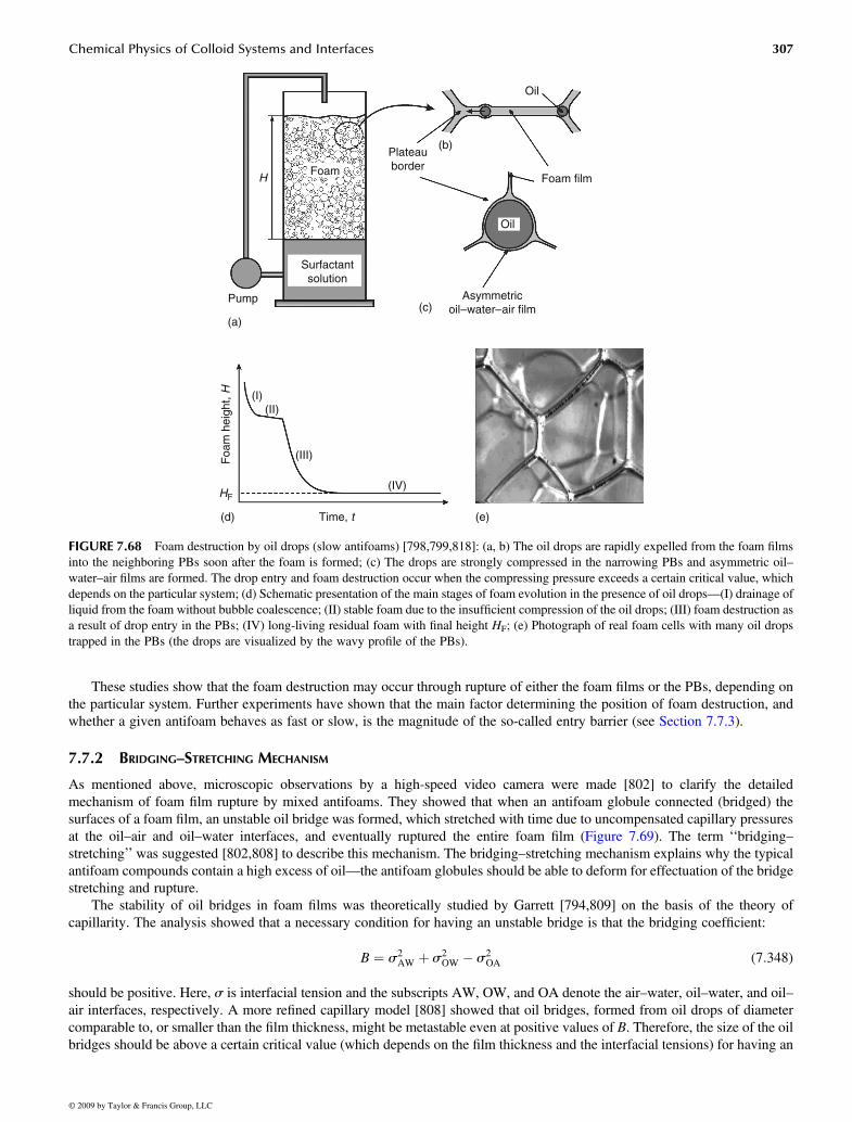
These studies show that the foam destruction may occur through rupture of either the foam films or the PBs, depending onthe particular system. Further experiments have shown that the main factor determining the position of foam destruction, andwhether a given antifoam behaves as fast or slow, is the magnitude of the so-called entry barrier (see Section 7.7.3).

7.7.2 BRIDGING–STRETCHING MECHANISM

As mentioned above, microscopic observations by a high-speed video camera were made [802] to clarify the detailedmechanism of foam film rupture by mixed antifoams. They showed that when an antifoam globule connected (bridged) thesurfaces of a foam film, an unstable oil bridge was formed, which stretched with time due to uncompensated capillary pressuresat the oil–air and oil–water interfaces, and eventually ruptured the entire foam film (Figure 7.69). The term ‘‘bridging–stretching’’ was suggested [802,808] to describe this mechanism. The bridging–stretching mechanism explains why the typicalantifoam compounds contain a high excess of oil—the antifoam globules should be able to deform for effectuation of the bridgestretching and rupture.

The stability of oil bridges in foam films was theoretically studied by Garrett [794,809] on the basis of the theory ofcapillarity. The analysis showed that a necessary condition for having an unstable bridge is that the bridging coefficient:

B ¼ s2AW þ s2

OW � s2OA (7:348)

should be positive. Here, s is interfacial tension and the subscripts AW, OW, and OA denote the air–water, oil–water, and oil–air interfaces, respectively. A more refined capillary model [808] showed that oil bridges, formed from oil drops of diametercomparable to, or smaller than the film thickness, might be metastable even at positive values of B. Therefore, the size of the oilbridges should be above a certain critical value (which depends on the film thickness and the interfacial tensions) for having an

FIGURE 7.68 Foam destruction by oil drops (slow antifoams) [798,799,818]: (a, b) The oil drops are rapidly expelled from the foam filmsinto the neighboring PBs soon after the foam is formed; (c) The drops are strongly compressed in the narrowing PBs and asymmetric oil–water–air films are formed. The drop entry and foam destruction occur when the compressing pressure exceeds a certain critical value, whichdepends on the particular system; (d) Schematic presentation of the main stages of foam evolution in the presence of oil drops—(I) drainage ofliquid from the foam without bubble coalescence; (II) stable foam due to the insufficient compression of the oil drops; (III) foam destruction asa result of drop entry in the PBs; (IV) long-living residual foam with final height HF; (e) Photograph of real foam cells with many oil dropstrapped in the PBs (the drops are visualized by the wavy profile of the PBs).




Pump

FoamH

Plateauborder

Foam film

Oil

Oil

(b)

(c)

(e)(d)

(a)

Time, t

(I)(II)

Foa

m h

eigh

t, H

(III)

(IV)

Surfactantsolution

Asymmetricoil–water–air film

HF

unstable oil bridge. This theoretical result was invoked to explain the reduced stability of the foam films in the presence of aspread oil layer (for details see Ref. [808]).

7.7.3 ROLE OF THE ENTRY BARRIER

Any mechanism of foam destruction by preemulsified antifoam globules requires an entry of these globules at the surface of thefoam film or the PB (e.g., Figures 7.68 and 7.69). The entry event depends on two major factors: (1) The equilibrium position ofan oil drop (lens) on the air–water interface, which is determined by the values of the interfacial tensions sAW, sOW, and sOA

(see Figure 7.11). (2) The repulsive forces (e.g., of electrostatic origin), which stabilize the asymmetric oil–water–air film,formed when an antifoam globule approaches the foam film surface; the barrier created by these forces should be overcome forthe globule entry to occur [794,796,800,801,810–814].

A theoretical analysis shows [794] that if the so-called entry coefficient:

E ¼ sAW þ sOW þ sOA (7:349)

is negative (as it is the case with some oils and surfactant solutions), the oil drops do not have a stable equilibrium position atthe surface and spontaneously submerge into the surfactant solution. Such oils are inactive as antifoams because no oil bridgescan be formed (factor 1 is decisive). One of the main reasons to use silicone oils in various antifoam formulations is that theseoils usually have positive values of B and E coefficients in the solutions of most conventional (hydrocarbon-based) surfactants[794,815]. Besides, it was theoretically shown that a positive value of B necessarily corresponds to a positive value of E (thereverse is not always true) [797,816].

The experiments show, however, that many oils with positive B and E coefficients might have low antifoam efficiency[798,799,806,807]. In these cases, the stability of the asymmetric oil–water–air films is very high, and the formation of unstableoil bridges becomes impossible for kinetic reasons (factor 2 is decisive). The repulsive interaction that should be overcome foreffectuation of the antifoam globules entry on the solution surface is usually termed ‘‘the entry barrier.’’ A recently developedmethod FTT [807,817,818] allowed one to quantify precisely the entry barrier with actual micrometer-sized antifoam globules,

FIGURE 7.69 Schematic presentation of the bridging–stretching mechanism of foam film rupture by antifoam globules [802,808]: After anoil bridge is formed (a–c), it stretches due to uncompensated capillary pressures at the oil–water and oil–air interfaces (c–e). Finally, thebridge ruptures in its thinnest central region (the vertical wavy line in e). The globule entry is possible only if the entry coefficient, E> 0, andthe entry barrier is low (see Section 7.7.3).




Foamfilm

Globule entry

Bridging

Stretching(d)

(b)

(a)

(c)

(e) Film rupture

E > 0Small barrier

and a number of important results have been obtained. The principle of the FTT and some of the main conclusions, drawn fromthe results obtained by this technique, are briefly discussed below.

7.7.3.1 Film Trapping Technique (FTT)

The principle and the experimental setup of the FTT are illustrated in Figure 7.70 [807,817,818]. Briefly, a vertical glasscapillary is positioned at a small distance above the flat bottom of a glass vessel. The lower end of the capillary is immersed inthe working surfactant solution which contains dispersed antifoam globules. The capillary is connected to a pressure controlsystem which allows one to vary and to measure the air pressure in the capillary, PA. When PA increases, the air–watermeniscus in the capillary is pushed against the glass substrate and a wetting film (glass–water–air) is formed which traps someof the antifoam globules. The setup allows one to determine the capillary pressure of the air–water meniscus around the trappeddrops, PC¼PA�PW, where PW is the pressure in the aqueous film (for details, see Refs. [817,818]). The experiments showthat the trapped antifoam globules enter (pierce) the surface of the wetting film at a given, critical capillary pressure, PCR

C .Therefore, the equipment allows one to measure PCR

C as a function of various parameters, such as the types of oil and surfactant,concentration of solid particles in the compound, size of the antifoam globules, etc. A larger value of PCR

C corresponds to ahigher entry barrier (more difficult drop entry) and vice versa. For compounds having very low entry barriers, a special versionof the FTT was developed [817] (gentle FTT) (see Figure 7.70c). Experiments in the presence and absence of a prespread oillayer can be performed, which allows one to evaluate the effect of oil spreading on the entry barrier.

7.7.3.2 Critical Entry Pressure for Foam Film Rupture

Experiments with a large set of systems (various oils, compounds, and surfactants) showed [800,818] that there is a well-defined threshold value, PTR� 15 Pa, which separates the fast (foam film breaking) from the slow (PB breaking) antifoams.Some of the results from these experiments are summarized in Figure 7.71, where the relationship between the foam lifetimeand the entry barrier, PCR

C , is shown. One sees from this figure that all experimental points fall into two distinct regions:(1) Systems in which the foam is destroyed for less than 10 s, i.e., these correspond to fast antifoams; for them PCR

C < 15Pa;(2) Systems for which the defoaming time is longer than 5 min (slow antifoams); for them PCR

C > 20Pa. Therefore, themagnitude of the entry barrier is of crucial importance for the time scale of foam destruction by oil-based antifoams. Anotherrelation of PCR

C with the antifoam activity (more precisely, with the height of the residual foam, HF, in the presence of oil drops;see Figure 7.68d) was discussed in Refs. [798,818].

One should note that at high surfactant concentrations, only oil–solid compounds have been observed to behave as fastantifoams, whereas both oils and compounds could behave as slow antifoams depending on the magnitude of the entry barrier(at low surfactant concentrations, the pure oils could also act as fast antifoams). In all experiments it was found that thehydrophobic solid particles reduce the entry barrier by one to two orders of magnitude, but sometimes PCR

C remains higher than

FIGURE 7.70 Scheme of the experimental setup and the basic principle of the FTT [817]. (a) Vertical capillary, partially immersed insurfactant solution containing antifoam globules, is held close to the bottom of the experimental vessel. (b) The air pressure inside thecapillary, PA, is increased and the convex air–water meniscus in the capillary is pressed against the glass substrate. Some of the antifoamglobules remain trapped in the formed glass–water–air film and are compressed by the meniscus. At a given critical capillary pressure,PCRC ¼ PA � PW, the asymmetric film formed between the antifoam globule and the solution surface ruptures and an event of globule entry is

observed by an optical microscope. (c) Another modification called gentle FTT is used for measuring entry barriers lower than 20 Pa—aninitially flat meniscus is formed, which allows the trapping of antifoam globules at a virtually zero capillary pressure.




Pressure control andmeasuring systems Capillary

PA

PWAir

(a)

(b)

(c)

Water

Antifoamglobule

Microscope

the threshold value, PTR, and the compound is unable to break the foam films. In the latter cases, the compound globules areexpelled into the neighboring PBs during the process of foam film drainage. These results confirm the idea of Garrett [794] thatthe main role of the solid particles in the antifoam compounds is to reduce the entry barrier of the globules.

7.7.3.3 Optimal Hydrophobicity of Solid Particles

Some authors accept [815,819] that the use of more hydrophobic solid particles results in more active antifoam compounds. In arecent study [805], this idea was experimentally tested by applying the following procedure for a gradual increase of silicahydrophobicity: initially hydrophilic silica particles were mixed with silicone oil at a room temperature, and this mixture wasstored under mild stirring for a long period of time. Under these conditions, the adsorption of silicone oil on the silica surface isa slow process which takes weeks before the final, most hydrophobic state of the particles is reached. The antifoam efficiency ofthe compound was tested every day, and the results obtained with various systems unambiguously showed the presence of awell pronounced, optimal silica hydrophobicity corresponding to highest antifoam efficiency.

The antifoam efficiency in these experiments was evaluated [805] by an automatic shake test. Briefly, 100 mL ofthe foaming solution was placed in a standard 250 mL glass bottle and 0.01% of the compound was introduced intothis sample. The bottle was then mechanically agitated in a series of consecutive shake cycles. After each cycle of agitationfor 10 s, the solution remained quiescent for another 60 s and the defoaming time was measured (defined as the time forappearance of a clean water–air interface without bubbles). Afterward, a new shaking cycle was performed and this procedurewas repeated until the defoaming time exceeded 60 s in three consecutive cycles—this was considered as the momentof compound exhaustion (see Section 7.7.4 and Figure 7.74 for further explanations). Larger number of cycles before thecompound exhaustion corresponds to better antifoam durability (efficiency) and vice versa.

The observed maximum (see the illustrative result presented in Figure 7.72a) was explained [805] as a result of tworequirements which stem from the main role of the silica particles, namely, to assist the globule entry by rupturingthe asymmetric oil–water–air films (see Figure 7.73). The first requirement, formulated by Garrett [794], is that the particlesshould be sufficiently hydrophobic to be dewetted by the oil–water and air–water interfaces (otherwise, the solidparticles would stabilize, rather than destabilize the asymmetric film). The other requirement [805] is that the particles shouldprotrude sufficiently deep into the aqueous phase in order to bridge the surfaces of the asymmetric oil–water–air film, and it isbetter satisfied by more hydrophilic particles. Therefore, an optimal hydrophobicity is expected, at which both requirements arebalanced, the entry barrier is low, and the antifoam is most active. Indeed, a straightforward correlation between the antifoamefficiency and the magnitude of the entry barrier, PCR

C , was observed in the studied systems (Figure 7.72b). For sphericalparticles, the optimal hydrophobicity was expressed as a most favorable three-phase contact angle solid–water–oil [805]:

cos uO � hAS=RP � 1 (7:350)

wherehAS is the thickness of the asymmetric oil–water–air filmRP is the particle radius (see Figure 7.73)

This angle corresponds to the condition hAS¼ dPR, where dPR¼RP(1þ cos uO) is the equilibrium protrusion depth of the solidparticle into the aqueous phase.

FIGURE 7.71 Correlation between the entry barrier, PCRC , and the foam lifetime measured for various surfactant–antifoam systems: The

experimental data (solid circles) fall into two distinct regions: systems in which the foam is destroyed in less than 5 s (fast antifoams) andPCRC < 15 Pa; and systems for which the defoaming time is longer than 8 min (slow antifoams) and PCR

C > 20 Pa. The composition of thevarious systems is given in Ref. [818].




10 100

Entry barrier PCCR (Pa)

100011

10

100

1000

Fast antifoams

Slow antifoams

PTR ~ 15 Pa

Foa

m li

fetim

e (s

)

7.7.3.4 Role of the Prespread Oil Layer

It has been known for many years [794,820,821] that some correlation exists between the spreading behavior of the oils andtheir antifoam activity. The value of the spreading coefficient:

S ¼ sAW � sOW � sOA (7:351)

which characterizes the mode of spreading of the oil on the surface of the solution, and the rate of oil spreading have been oftenconsidered as important factors for the antifoam activity. However, as shown by Garrett et al. [822] the oil spreading is not anecessary condition for having an active antifoam, and many studies [798,799,806] have confirmed that the correlation is notalways present.

The effect of the spread oil on the entry barriers of various oils and oil–silica compounds was studied by the FTT[800,804,807]. The experimental results showed that the presence of a prespread oil layer on the surface of the solution reducesby several times the entry barrier for mixed oil–silica compounds (see Table 7.9). Furthermore, it was found [804] that theentry barrier in many systems is below the threshold value PTR� 15 Pa (which separates the fast from slow antifoams, seeFigure 7.71), only in the presence of a prespread layer of oil. In other words, these antifoams behave as fast ones only becausethe oil spreads rapidly on the solution surface during foaming, reducing in this way the entry barrier below PTR. The resultsfor the entry barrier of oil drops (without silica) also showed a moderate reduction of the entry barrier by a prespread oil in mostsystems [804,807]. However, at least in one of the studied systems (hexadecane drops in solutions of the anionic surfactantsodium dodecyl-benzenesulfonate; see Table 7.9) a significant increase of the entry barrier upon oil spreading was

0

(a)

(b)

0

20

40

60

Ant

ifoam

effi

cien

cy(d

urab

ility

), n

umbe

r of

cyc

les

80

100

0

0 5 10

Critical pressure to entry (Pa)

Crit

ical

pre

ssur

e to

ent

ry (

Pa)

15 20

5

10

15

20

25

0

20

40

60

80

100

100 200 300 400 500

AOT

Time for silica hydrophobization (h)

Ant

ifoam

effi

cien

cy(d

urab

ility

), n

umbe

r of

cyc

les

600 700 800

AOT

APG

Triton

900

FIGURE 7.72 (a) Critical pressure for globule entry, PCRC (full circles), and efficiency (empty circles) of a silicone oil–silica compound in 10

mM AOT solution, as functions of the time of silica hydrophobization. (b) The dependence of the compound efficiency on PCRC for solutions

of three different surfactants: 10 mM anionic AOT, 0.6 mM nonionic APG; and 1 mM nonionic Triton X-100. (Adapted from Marinova,K.M., Denkov, N.D., Branlard, P., Giraud, Y., and Deruelle, M., Langmuir, 2001 [805]. With permission.)




observed [807]. The entry barrier of the oils in surfactant solutions above their critical micellization concentration (CMC) ishigher than PTR both in the presence and absence of spread oil, which explains why the pure oils behave as slow antifoams attypical surfactant concentrations.

We can conclude from the results shown in Table 7.9, that there is a well-pronounced synergistic effect between the solidparticles present in compounds and the spread oil. Most of the studied fast antifoams have sufficiently low entry barriersexclusively as a result of the combined action of the solid particles and the spread oil layer [804].

As mentioned in Section 7.7.2, the spread layer of oil has another important role as well. The spread oil is able to feedthe oil bridges, formed in foam films, by a mechanism explained in Ref. [808], as a result, larger and less stable oil bridgesare formed.

7.7.4 MECHANISMS OF COMPOUND EXHAUSTION AND REACTIVATION

The process of antifoam exhaustion (deactivation) is illustrated in Figure 7.74—the time for foam destruction in a standardshake test is shown as a function of the number of the shaking cycle (see Section 7.7.3.3 for the used shake test) [823]. Shorterdefoaming time means more active antifoam and vice versa. As seen from Figure 7.74, the initial high activity of the antifoamdeteriorates with the foaming cycles and the defoaming time becomes longer than 60 s after 45 cycles—the antifoam has beenexhausted. This process is very undesired from practical viewpoint, and more durable antifoams (able to sustain a larger numberof foam destruction cycles) are searched by the manufacturers.

Aqueous film

Asymmetric film

Asymmetric film

Antifoamglobule

Air

Air

hAS

hAS dPR

Air

Air

Oil

Oil

Solid

(b)

(c)

(a)

qO

qA

qO

Solid

FIGURE 7.73 Schematic explanation of the optimal hydrophobicity of the solid particles in oil–solid antifoam compounds: (a) When anantifoam globule approaches the foam film surface, an asymmetric oil–water–air film of thickness hAS forms. (b) The zone of contact in anenlarged scale. If the protrusion depth, dPR, of the solid particle is larger than hAS, the particle should be sufficiently hydrophobic(uAþ uO> 1808) in order to pierce the air=water interface and induce a film rupture; however, if the particle is insufficiently hydrophobic(uAþ uO< 1808), it would stabilize the film [794]. (c) On the other side, if the solid particles is over-hydrophobized, then dPR< hAS and theparticle is again unable to pierce the asymmetric film [805].




Interestingly, the addition of a new portion of oil (without silica particles) leads to a complete restoration of the antifoamactivity (Figure 7.74). Note that the oil itself has a very weak antifoam activity in the absence of silica. Therefore, the antifoamreactivation certainly involves the solid particles that have been introduced with the first portion of mixed antifoam. Thesubsequent foaming cycles lead to a second exhaustion series, and such consecutive periods of exhaustion=reactivation can berepeated several times.

TABLE 7.9Entry Barriers, PCR

C , of Different Antifoams in Surfactant Solutionsin the Presence and Absence of a Prespread Layer of Oil, fromwhich the Antifoam is Prepared

Antifoam Surfactant Spread Layer PCRC , Pa

Dodecane 2.6 mM SDDBS No 96� 5Yes 48� 5

Hexadecane 2.6 mM SDDBS No 80� 5

Yes 400� 10Silicone oil 10 mM AOT No 28� 1

Yes 19� 2Compound 1 10 mM AOT No 8� 1

Yes 3� 2Compound 2 10 mM AOT No 20� 5

Yes 4� 1

Compound 1 1 mM Triton X-100 No 30� 1Yes 5� 2

Compound 2 1 mM Triton X-100 No 22� 1

Yes 7� 1

Sources: Data from Denkov, N.D., Tcholakova, S., Marinova, K., and Hadjiiski, A., Role of oilspreading for the efficiency of mixed oil-solid antifoams, Langmuir, 2001. submitted;Hadjiiski, A., Tcholakova, S., Denkov, N.D., Durbut, P., Broze, G., and Mehreteab, A.,

Langmuir, 17, 7011, 2001.Notes: SDDBS and AOT denote the anionic surfactants sodium dodecyl-benzenesulfonate and sodium

dioctyl-sulfosuccinate, respectively. Triton X-100 is the nonionic surfactant nonylphenol deca

(ethyleneglycolether). Compound 1 is a mixture of silicone oil and hydrophobized silica;Compound 2 is an emulsion of Compound 1, which contains also solid particles of Span 60.

FIGURE 7.74 Consecutive cycles of exhaustion and reactivation of mixed oil–silica compound in 10 mM solution of the anionic surfactantsodium dioctyl-sulfosuccinate (AOT). An initially active antifoam (defoaming time� 5 s) gradually looses its activity with the number offoam formation=destruction cycles in a standard shake test [823]. The introduction of silicone oil results in a perfect restoration of the antifoamactivity. Five exhaustion curves (indicated by roman numbers; the symbols indicate the experimentally measured defoaming time) and thecorresponding four reactivation events (the vertical dashed lines) are shown. (Adapted from Ref. [823].)




100

I II III IV V

Number of foam formation/destruction cycles

Tim

e fo

r fo

am d

estr

uctio

n (s

)

150 20000

10

20

30

40

50

60

Added5 µL oil

Added5 µL oil

Added5 µL oil

Added5 µL oil

50

Systematic experiments [823] with solutions of the anionic surfactant sodium dioctyl-sulfosuccinate (AOT) showed that theexhaustion of mixed silica–silicone oil antifoams is due to two closely interrelated processes: (1) partial segregation of the oiland silica into two distinct, inactive populations of antifoam globules, silica-free and silica-enriched; (2) disappearance of thespread oil layer from the solution surface (Figure 7.75). The oil drops deprived of silica, which appear in process 1, are unableto enter the air–water interface and to destroy the foam lamellae, because the entry barrier is too high for them. On the otherhand, the antifoam globules enriched in silica trap some oil, which is not available for spreading on the solution surface. As aresult, the spread oil layer gradually disappears from the solution surface (process 2) due to oil emulsification in the moment offoam film rupture. Ultimately, both types of globules, silica-enriched and silica-free, become unable to destroy the foam films,and the antifoam transforms into an exhausted state. Accordingly, the reactivation process is due to: (1) restoration of the spreadoil layer, and (2) rearrangement of the solid particles from the exhausted antifoam with the fresh oil into new antifoam globuleshaving optimal silica concentration. No correlation between the size of the antifoam globules and their activity was establishedin these experiments, which showed that the reduction of the globule size (which is often considered as the main factor in theantifoam exhaustion) was a second-order effect in the studied systems. Similar conclusions were drawn from experiments withnonionic surfactants as well [803].

In conclusion, a progress has been achieved during the last years in revealing the mechanisms of foam destruction by oil-based antifoams. This progress has been greatly facilitated by the various methods for direct microscopic observations of thefoams and foam films (including some of the foam destruction events), and by the implementation of the FTT for a directmeasurement of the entry barriers of the antifoam globules.

7.8 ELECTROKINETIC PHENOMENA IN COLLOIDS

The term ‘‘electrokinetic phenomena’’ refers to several processes which appear when a charged surface (or colloidal particle) isset in a relative motion with respect to the adjacent liquid phase. Classically, four types of electrokinetic phenomena aredistinguished: electroosmosis, streaming potential, electrophoresis, and sedimentation potential (Figure 7.76). These will bediscussed in Sections 7.8.2 through 7.8.6. Nowadays, the electrical conductivity (at constant electrical field) and the dielectricresponse (at alternating electrical field) of the disperse systems are often considered together with the electrokinetic phenomena,because the theoretical approaches and the governing equations are similar (Section 7.8.7). Experimental methods based on allthese phenomena are widely used for characterization of the electrical surface potential in dispersions. A comprehensivepresentation of the topic until the end of 1980s can be found in review articles [824–834] and monographs [835–837].

FIGURE 7.75 Schematic presentation of the processes of antifoam exhaustion and reactivation of emulsified oil–silica antifoam compound.




Globules: Optimal silica/oilratio

Globules: Silica-rich and silica-free (both inactive)

Active Antifoam

Foaming

Additionof PDMS

Reactivation

Exhausted Antifoam

Introduction of PDMS

Reactivated AntifoamGlobules: Optimal silica/oil

ratio

Globules: redistribution

Spread oil layer: Yes

Spread oil layer: No

spread oil layer: Yes

Spread oil layer: Yes

The recent development of the area is reviewed in the collective monograph [838]. The major experimental techniques aredescribed in Chapter 4 of Ref. [836] and Chapters 8 through 14 in Ref. [838]. Recently, a substantial interest has been raised bythe apparent discrepancy between the results obtained by different electrokinetic methods for one and the same system. Thisproblem is discussed in Section 7.8.8. Finally, the electrokinetic properties of air–water and oil–water interfaces are brieflydescribed in Section 7.8.9.

7.8.1 POTENTIAL DISTRIBUTION AT A PLANAR INTERFACE AND AROUND A SPHERE

When a dielectric phase (solid or fluid) is placed in contact with polar liquid, such as water, the interface gets charged due toeither specific adsorption of ions initially dissolved in the polar liquid, or dissociation of surface ionizable groups [14,34,837].The final result of these two processes is the formation of an electrical double layer (see Figure 7.77), which may contain threetypes of ions:

1. Ions attached to the surface by chemical bond are those parts of the ionized groups which remain bound after thedissociation process.

2. Ions bound by very strong Coulomb attraction (after partial loss of molecules from the ion solvating shell) or by someother noncovalent specific, short-range attraction build up the so-called Stern layer.

3. Ions that are involved in more or less free Brownian motion present the diffuse part of the electrical double layer.

The ions from groups (1) and (2), considered together, determine the effective surface charge density, ss, which must bebalanced by an excess of counterions in the diffuse layer (equal in magnitude and opposite in sign). The distribution ofelectrical potential in the diffuse layer is usually rather accurately described by the Poisson–Boltzmann (PB) equation:

r2c ¼ � e

««0

Xj

Zjnb,j exp � eZjc

kT

� �(7:352)

wherec is the local (average) value of the electrical potentiale is the elementary charge« is the relative dielectric permittivity of the liquid«0 is the electrical permittivity in vacuoZj and nb,j are the number of charges and the bulk number concentration, respectively, of ion j

Drivingforce

Movingphase

Solid phase isImmobile

Solid particles (orliquid droplets)

are moving

(a) Electroosmosis

Electric field createsmechanical flux

– +

Mechanical fluxcreates electric field

2r2rP1 P2

∆j

∆j

(b) Streaming potential

(d) Sedimentation potential(c) Electrophoresis

FIGURE 7.76 The four basic electrokinetic phenomena: (a) Electroosmotic liquid flow through a capillary (of charged walls) appears whenan electric potential difference is applied; (b) Streaming electric potential appears when a pressure drop drives the liquid to flow through thecapillary; (c) Electrophoretic motion of charged particles is observed in an external electric field; (d) Sedimentation potential is establishedwhen charged particles are moving under the action of gravity.




The model of the electrical double layer based on Equation 7.352 is called in the literature Gouy–Chapmen or Gouy–Sternmodel. For symmetrical (Z:Z) electrolyte, the PB equation can be written in the form:

r2c ¼ 2eZn0««0

sinheZc

kT

� �(7:353)

where n0 is the bulk electrolyte number concentration. For a flat interface (see Figure 7.77), Equation 7.353 has an exactanalytical solution [34,368,837]:

c(x) ¼ 2kTeZ

ln1þ gs exp (�kx)

1� gs exp (�kx)

� �(7:354)

where

gs � tan hzecs

4kT

� �, k2 � 2e2Z2n0

««0kT

and cs is the electrical potential at the surface of closest approach of the ions from the diffuse layer to the interface. This surfaceis called the outer Helmholtz plane and cs is called the surface potential. The surface charge and potential are interrelated by theexpression:

ss ¼ �««0dc

dx

� �x¼0

¼ (8««0kTn0)1=2 sinh

eZcs

2kT

� �(7:355)

which is a direct corollary [14,34] from Equation 7.353 and the condition for overall electroneutrality of the interface.If the surface potential is small, one can expand in series the logarithm in the right-hand-side of Equation 7.354 and derive

the Debye–Hückel equation:

Shear plane

Ions in thediffuse layerIons in the

stern layer

Ionizedsurface group

0xs x

y

ysz

OHP

–

–

––

––

++

+

++

FIGURE 7.77 Schematic presentation of the structure of the electrical double layer (EDL). The surface charge is created by ionized surfacegroups and=or by ions tightly adsorbed in the Stern layer. The plane of closest approach of the ions from the diffuse part of the electricaldouble layer is called the outer Helmholtz plane (OHP). The electric potential in the OHP plane is referred to as the surface potential, cs, inthe text. The shear plane, x¼ xs, separates the hydrodynamically immobile liquid that moves together with the surface, x< xs, from the mobileliquid, x> xs, which has nonzero relative velocity with respect to the surface. Note that the ions in the immobile part of the EDL can movewith respect to the surface under an applied electric field, which gives rise to the anomalous surface conductivity (Section 7.8.8).




c(x) ¼ cs exp (�kx),Zecs

kT< 1 (7:356)

On the other hand, the potential always decays exponentially far from the interface (kx � 1) at an arbitrary magnitude of cs

(see Equation 7.354):

c(x) ¼ 4kTeZ

gs exp (�kx), kx � 1 (7:356a)

The potential distribution around a spherical particle can be found from the PB equation (Equation 7.352), which in thiscase reads:

1r2

d

drr2dc

dr

� �¼ � e

««0

Xj

Zjnb,j exp � eZjc(r)

kT

� �(7:357)

The respective boundary conditions are

c(r ¼ R) ¼ cs, c(r ! 1) ¼ 0

Equation 7.357 has an analytical solution only in the case of small surface potential:

c(r) ¼ cs

R exp [�k(r � R)]

r,

Zecs

kT< 1 (7:358)

In this case, the surface charge density is a linear function of cs:

ss ¼ ««0(1þ kR)

Rcs,

Zecs

kT< 1 (7:359)

For a large surface potential, cs, the potential distribution can be found by numerical integration of the PB equation. Far fromthe sphere surface, the potential always obeys the law:

c(r) ¼ cs*R exp [�k(r � R)]

r, k(r � R) � 1 (7:360)

where cs*(kR,cs) is an effective potential, which can be found by numerical solution of the PB equation. By using the method

of matched asymptotic expansions, Chew and Sen [839] obtained for a thin electrical double layer (kR> 1):

cs* ¼ 4kT

Zegs þ

g3s

2kR

� �(7:361)

A useful relationship between cs and ss for a sphere was proposed by Loeb et al. [840]:

ss ¼ ««0kkT

Ze2sin h

Zecs

2kT

� �þ 4

kRtan h

Zecs

4kT

� �� (7:362)

and was theoretically justified by other authors [838,841–844]. Equation 7.362 coincides with the exact numerical resultswithin an accuracy of a few percent for kR> 0.5 and arbitrary surface potential [836,840]. A general approach for derivation ofapproximate (but accurate) expressions relating cs and ss, including for systems containing nonsymmetric electrolytes, hasbeen proposed by Ohshima [844,845].

7.8.2 ELECTROOSMOSIS

When an electrical field of intensity E is applied in parallel to a charged flat interface, the excess of counterions in the diffuselayer gives rise to a body force exerted on the liquid. The liquid starts moving with local velocity varying from zero in the planeof shear (x¼ xs) to some maximal value, VEO, at a large distance from the wall (see Figure 7.77). The magnitude of thiselectroosmotic velocity was calculated by Smoluchowski [846] under the assumptions that: (1) the ion distribution in the




diffuse layer obeys the PB equation, (2) at each point the electrical force is balanced by the viscous friction, and (3) the liquidviscosity in the diffuse layer is equal to that of the bulk liquid, h. The final result reads [846]:

VEO ¼ � ««0z

hE (7:363)

where z is the electrical potential in the shear plane, i.e., z � c(x¼ xs). The quantity

mEO ¼ VEO

E¼ � ««0z

h(7:364)

is called electroosmotic mobility. The Smoluchowski consideration is also applicable to capillaries of a radius much larger thanthe Debye screening length, k�1. Therefore, by measuring the liquid flow through a capillary, like that shown in Figure 7.76,one can determine the z potential of the capillary surface. It is usually acceptable [836] to measure the liquid flux (volumedisplaced per unit time), JEO, along with the electric current transported by the liquid, IEO:

JEO ¼ pr2VEO and IEO ¼ pr2xbE (7:365)

wherer is the capillary radiusxb is the bulk conductivity of the liquid

The ratio

JEO IEO ¼ VEO xbE ¼ � ««0z

hxb(7:366)

does not depend on the capillary radius and can be used to determine z. Quite often, however, the high concentration of ions inthe double electric layer leads to a much higher conductivity in the surface region, compared to that in the bulk electrolytesolution. To account for this effect Bikerman [847] introduced the term ‘‘specific surface conductivity,’’ xs, which presents anexcess quantity over the bulk conductivity. Then, Equation 7.365 is modified to read:

IEO ¼ (pr2xb þ 2prxs)E (7:367)

and Equation 7.366 acquires the form:

jJEO=IEOj ¼ ««0z

h(xb þ 2xs=r)(7:368)

Alternatively, instead of measuring the electroosmotic liquid flux at zero pressure difference across the capillary, one candetermine [836] z by measuring the counterpressure, DPEO, necessary to completely stop the net liquid transport through thecapillary:

DPEO ¼ 8««0zpr4(xb þ 2xs=r)

IEO (7:369)

Bikerman [847] obtained the following expression for xs in the case of a symmetrical (Z:Z) electrolyte, under the assumptionthat the surface conductivity is due only to the ions located in the movable part of the diffuse layer:

xs ¼2Z2e2n0kTk

Dþ exp � Zez

2kT

� ��1

� �1þ 3mþ

Z2

� �þ D� exp

Zez

2kT

� ��1

� �1þ 3m�

Z2

� �� (7:370)

where D� are ion diffusion coefficients, while m� are dimensionless ion mobilities, defined as

m� ¼ 23

kT

e

� �2««0h

Z2

D� ¼ 2««0NAkT

3hZ2

L0 ¼ 12:84� 10�4 Z2

L0

� �at 25 C in water (7:371)




L8 (m2 ohm�1 mol�1) is the limiting molar conductivity of ions at infinite dilution. The typical values of xs are around10�9 ohm�1. For comparison, the bulk conductivity, xb, is given by

xb ¼e2

kT

XDjZ

2j nb,j (7:372)

and can vary within a wide range (note that xs and xb have different dimensions).Equation 7.368 shows that for determination of z and xs, one needs measurements with several capillaries made of the same

material, but having different radii. The effect of the surface conductivity can be neglected when the criterion

2xs

xbr� 1

krexp

Zecs

2kT

� �� 1 (7:373)

is satisfied [836,837,848]. In other words, the surface conductivity is negligible at low surface potential and high ionic strength.Besides, Equation 7.366 can be applied [836,848,849] also to electroosmotic flow in porous plugs or membranes if: (1) thetypical pore size is much larger than k�1 (2) the effects of the surface conductivity, xs, are negligible, and (3) the flow islaminar.

This consideration can be extended to include capillaries of radii comparable to k�1 and the cases when the potentialdistribution cannot be approximated using the results for a planar wall [827,836].

The so-called plane interface technique [850–852] is a modification of the electroosmotic method, in which submicrometerparticles are used as probes to visualize the osmotic velocity profile close to an interface. The method allowed precisedetermination of the z potential at mica, quartz, sapphire, and fused-silica surfaces as a function of pH [851,852]. The attempt[850,852,853] to apply the plane interface technique to the air–water interface, however, gave ambiguous results, probably dueto the interfacial fluidity.

7.8.3 STREAMING POTENTIAL

If a pressure drop, DP¼P1�P2, is imposed at the ends of a capillary, like that shown in Figure 7.76, the liquid starts movingthrough the capillary [836,843]. The charges in the mobile part of the double layer at the capillary wall are thus forced to movetoward the end of the capillary. As a result, a streaming current, IST, appears which leads to the accumulation of excess charge atthe capillary end. This excess charge gives rise to an electric potential difference between the ends of the capillary, calledstreaming potential, EST. On its own, the streaming potential causes a current flow, IC, in a direction opposite to IST. Finally, asteady state is established when jICj ¼ jISTj and the net electric current across the capillary becomes zero. One can directlymeasure EST by probe electrodes, and the following relationship is used to determine the z potential of the capillary walls [836]:

EST

DP¼ ««0z

h(xb þ 2xs=r)(7:374)

Alternatively, instead of measuring EST, one can measure the streaming current, IST, by using the appropriate electricalcircuit [836]:

IST ¼ � ««0h

pr2

LDPz (7:375)

where, L denotes the length of the capillary. An important advantage of the streaming current measurement is that the surfaceconductivity does not matter for the calculation (see Equation 7.375), and experimental determination of xs is not necessary.Similar experiments were performed by Scales et al. [854] to determine the z potential of mica surface.

Equations 7.374 and 7.375 are valid only if the capillary radius is much larger than the thickness of the diffuse layer.A number of modifications were suggested in the literature to extend the theoretical consideration to narrower capillaries andporous plugs (see, for example, the review article by Dukhin and Derjaguin [827] and the book of Hunter [836]). Measurementsof the streaming potential, streaming current, and electrical conductance of plugs made of latex particles were performed andanalyzed by van den Hoven and Bijsterbosch [855].

7.8.4 ELECTROPHORESIS

The movement of a charged colloidal particle in an external electrical field is called electrophoretic motion and the respectivephenomenon is electrophoresis. The electrophoretic velocity in the two limiting cases, of a thin and thick electrical double layeraround a spherical particle, can be calculated by Smoluchowski [856] and Hückel [857] formulas:




VEL ¼ ««0z

hE, kR � 1 (Smoluchowski) (7:376)

VEL ¼ 23««0z

hE, kR � 1 (Huckel) (7:377)

It is important to note that Equation 7.376 is valid for particles of arbitrary shape and size, if the following requirement isfulfilled: The dimensions of the particle and the local radii of curvature of the particle surface are much larger than the Debyescreening length.

The problem for spherical particles at arbitrary kR was solved by Henry [858] who obtained

mEL ¼ VEL

E¼ 2

3««0z

hf1(kR) ¼ Q

6phR(1þ kR)f1(kR) (Henry) (7:378)

wheremEL is the particle electrophoretic mobilityQ is the particle chargef1(kR) is a correction factor given by

f1(kR) ¼ 32� 92(kR)�1 þ 75

2(kR)�2 � 330(kR)�3, kR > 1

f1(kR) ¼ 1þ 116

(kR)2 � 548

(kR)3 � 196

[(kR)4 � (kR)5]

þ 18(kR)4 � 1

96(kR)6

� �exp (kR)E1(kR), kR < 1 (7:379)

and E1(x) �Ð11 e�sxds

s is an integral exponent of the first order. The limiting values, f1(kR ! 1)¼ 3=2 and f1(kR ! 0)¼ 1,reduce Henry’s equation to the equations of Smoluchowski and Hückel, respectively. The effect of the surface conductivity, xs,can be phenomenologically included in this approach, as shown by Henry [859]. Also, if the material of the particle has finiteelectrical conductivity, xp, its electrophoretic mobility is given by [858]:

mEL ¼ 23««0z

hf2(kR,xp=xb) (7:380)

where

f2(kR,xp=xb) ¼ 1þ 2(xb � xp)

(2xb þ xp)[f1(kR)� 1] (7:381)

It was shown [827,828,835], however, that the approach of Henry is strictly valid only for small values of the z potential,Zez=kT< 1, because it neglects the relaxation and the retardation effects, connected with distortion of the counterionatmosphere around the moving particle. Solutions of the problem for not-too-high z potentials were suggested by Overbeek[860] and Booth [861]. The mobility of a spherical, nonconducting particle of arbitrary z potential and arbitrary kR wasrigorously calculated by Wiersema et al. [862] and by O’Brien and White [863]. In Figure 7.78, the results of O’Brien andWhite [863] for the particle mobility as a function of the z potential at different values of kR are represented. One interestingconclusion from these calculations is that the mobility has a maximum for kR> 3, i.e., a given value of mEL may result fromtwo different values of z. The maximum in these curves appears at z �150 mV. The numerical algorithm of O’Brien and White[863] is sufficiently rapid to allow application to individual sets of experimental data.

Explicit approximate expressions were suggested by several authors. For a thin electrical double layer, Dukhin andDerjaguin [827] derived a formula, which was additionally simplified (without loss of accuracy) by O’Brien and Hunter [864]:

mEL ¼ ««0h

z � 4««0kT

e

ez2 � ln 2

Z 1� exp �Zez� �h i

2þ kReM exp � Zez2

� �8>><>>:

9>>=>>;, kR � 1 (7:382)




whereez � ezkT is the dimensionless z potential, eM ¼ (1þ 3m=Z2)

m is the dimensionless mobility of the ions (see Equation 7.371)

Equation 7.382 was derived assuming equal valency and mobility of the counter- and coions. The comparison with the exactnumerical calculations showed that Equation 7.382 is rather accurate for kR> 30 and arbitrary z potential. Another explicitformula of high accuracy (less than 1% for arbitrary z potential) and wider range of application (kR> 10) was suggested byOhshima et al. [865]

For low values of the z potential, Ohshima [866] suggested an approximate expression for the Henry’s function (Equations7.378 and 7.379), which has a relative error of less than 1% for arbitrary values of kR:

mEL ¼ 23««0z

h1þ 1

2{1þ 2:5=[kR(1þ 2e�kR)]}3

� �(7:383)

Recently, Ohshima [867] derived an extension of Equation 7.383, which is accurate for ez < 3 at arbitrary values of kR.The electrophoretic mobility of particles having a cylindrical or ellipsoidal shape was studied theoretically by Stigter [868],

van der Drift et al. [869], and Ohshima [870]. The polyelectrolytes [871–873] and the spherical particles covered by a layer ofpolymer [874,875] (or polyelectrolyte) are two other types of systems that have been matters of great interest. In a recent seriesof papers Ohshima and Kondo [876–878] derived a general analytic formula for the case of a hard particle, covered by a layerof polyelectrolyte. In the corresponding limiting cases, the general expression reduces to the known expressions for a hardspherical particle, a plate-like particle covered by a polyelectrolyte layer, or a charged porous sphere [876,877].

Churaev and Nikologorskaja [879] performed measurements of the electrophoretic mobility and the diffusion coefficientof silica particles before and after adsorption of polyethylenoxides. They found that the experimental data can be explainedonly by assuming that the adsorbed polymer layer not only shifts the shear plane apart from the particle surface (thus increasingthe hydrodynamic radius of the particles) but also substantially reduces the particle surface potential. According to the authors[879] the decrease in the surface charge could be due to the lower dielectric permittivity in the adsorption layer compared tothat of water. It is rather possible that a similar effect played a role in the experiments of Furusawa et al. [880] who showed thatthe adsorption of hydroxylpropylcellulose on latex particles may completely shield their charge (the particle z potentialbecomes zero). Since the adsorption layer was shown to be very stable in a wide range of pH and electrolyte concentrations,such particles can be used as a reference sample for electrophoretic measurements. These particles exactly follow theelectroosmotic liquid flow in the cell and, hence, represent a convenient probe sample for the plane interface techniquementioned in Section 7.8.2.

60.01

0.1

250kR = ∞kR = 0 150

100

70605040

30

20

1510

864

3

0.2

0.30.40.50.751.02.0

2.75

5

4

3

2

1

0

7

6

5

4

3

2

1

05 5 10

(a) (b)

7

z~

z~

m EL

~ m EL

~FIGURE 7.78 The dimensionless electrophoretic mobility of spherical particles, ~mEL ¼ 3 hemEL=(2««0kT), versus the dimensionless zeta-potential, ~j ¼ ez=(kT), for various values of kR: (a) kR varies between 0 and 2.75; (b) kR varies between three and infinity [863].




The effect of the interparticle interactions on the electrophoretic mobility in concentrated dispersions was theoreticallystudied by Levine and Neale [881]. They used a cell model with two alternative boundary conditions at the cell boundary todescribe the hydrodynamic flow: the free surface model of Happel [882] and the zero vorticity model of Kuwabara [883]. Theresults [881] suggested that the zero vorticity model is more appropriate, because it represents in a more correct way the limit tolow particle concentration. Experiments at very low electrolyte concentrations, when the electrostatic interactions between theparticles are very strong, were performed by Deggelmann et al. [884]. They observed a strong increase in the electrophoreticmobility at lower ionic strength (when the electrostatic interaction is stronger and the particles form a liquid-like structure)which was in apparent contradiction with the predictions of the Levine and Neale’s theory [881]. One possible explanation ofthis surprising result could be that the decrease of the ionic strength leads to a simultaneous increase in the surface potential[34], and this effect prevails over the increased interparticle interactions. Further development of the electrokinetic theory forconcentrated dispersions was presented by Kozak and Davis [885], and Ohshima [877,886].

Another interesting experimental study of concentrated suspensions of human erythrocytes was performed by Zukoski andSaville [887]. Although volume fractions as high as 75% were employed, the electrophoretic mobility changed by the factor(1�f) in the whole concentration range, which was simply explained by the backflow of liquid necessary to conserve thesuspension volume. The electrostatic and hydrodynamic particle–particle interactions apparently canceled each other in theseexperiments. One should note that the electrolyte concentration was relatively high and, contrary to the experiments ofDeggelmann et al. [884] the electrical double layers were thin in comparison with the particle size.

A recent progress was achieved in the theoretical description of the electrophoretic mobility of spherical particles inoscillating electrical field [888], the so-called dynamic mobility (see also Section 7.8.7.2). General equations at an arbitraryfrequency, z potential, and kR, as well as analytical formulas for low z potentials, were derived by Mangelsdorf and White[888]. Theory and experiment [889] demonstrated rather strong frequency dependence of the electrophoretic response of theparticles in the hertz and kilohertz regions. A general theoretical expressions, along with explicit approximate formulas, for thedynamic electrophoretic mobility of spheres and cylinders were derived by Ohshima [877,890,891]. The electrophoreticmeasurements in oscillating fields are stimulated also by the fact that the undesirable effect of the electroosmotic flow in theexperimental cell, created by the charge at the cell walls, is strongly suppressed in this type of equipment [889,892].

Another important recent development is the construction of equipment capable of measuring the mobility of nanometer-sized particles, such as micelles and protein molecules. The different mobility of proteins in polymer gels is widely usedfor their separation and identification [893], but this method is not suitable for the physicochemical study of proteins, becausethe interactions of the protein molecules with the polymer gel matrix could be rather specific. For a long time theelectrophoretic mobility of proteins in a free solution was studied by the moving boundary method of Tiselius [894], sinceelectrophoretic equipment based on DLS (Section 7.9.2.1) is limited to particles of a size between approximately 50 nm and10 mm. The method of Tiselius is not so easy and, in principle, it is not very suitable for micellar solutions, because aboundary between solutions of different concentrations must be formed. Imae et al. [895,897–900] described an improvedversion of electrophoretic light scattering equipment applicable to particles of a diameter as small as several nanometers.The feasibility of this equipment was demonstrated [896] by measuring the electrophoretic mobility of micelles of sodiumdodecylsulfate (SDS) and of mixed micelles of SDS with nonionic surfactants. The electrokinetic properties of micelles arediscussed in the recent review by Imae [900]. This experimental advance is accompanied by progress in the theoreticalanalysis of the electrophoretic mobility of nonspherical and nonuniformly charged particles (such as proteins) with somespatial charge distribution on the particle surface [901–904]. One quite interesting conclusion from the work of Yoon [904]was that Henry’s formula, Equations 7.378 through 7.379, is correct for spherical particles of arbitrary charge distribution(with Q being the net particle charge in this case), provided that the electrical potential is low and can be described by thelinearized PB equation.

More details about the method of electrophoretic mobility measurement by means of DLS are given in Section 7.9.2.1.

7.8.5 SEDIMENTATION POTENTIAL

When a charged particle is sedimenting under the action of gravity (Figure 7.76d) the ions in the electrical double layer are notobliged to follow the particle motion. Instead, a continuous flow of ions enters the lower half of the particle diffuse layer andleaves its upper half. The net effect is a spatial separation of the negative and positive charges which creates the sedimentationpotential of intensity, ESED. At a steady state, the electrical current caused by the particle motion must be counterbalanced by anequal-in-magnitude (but opposite-in-direction) current created by ESED. The intensity, ESED, can be directly measured by meansof electrode probes placed at two different levels in the suspension of settling particles. Smoluchowski [905] derived thefollowing equation connecting ESED and the z potential of spherical non conducting particles:

ESED ¼ ««0h

Fgrp

xb

at kR � 1 (7:384)




whereFg¼ gVp(dp� d0) is the gravity force (with subtracted Archimedes’ force) acting on a particlerp is the particle number concentration; g is gravity accelerationVp is the particle volumedp is the particle mass densityd0 is the mass density of the disperse medium

Generalization of the theoretical consideration to arbitrary values of kR was given by Booth [906]. The theory was later refinedby Ohshima et al. [907] who performed exact numerical calculations and proposed explicit formulas for the cases of not-too-high surface potential and for thin electrical double layers. The effect of particle concentration was considered by Levine et al.[908] who used a cell model to account for the hydrodynamic interaction between the particles. The theory of Levine et al.[908] is restricted to thin double layers (kR> 10) and low surface potentials.

7.8.6 ELECTROKINETIC PHENOMENA AND ONZAGER RECIPROCAL RELATIONS

All electrokinetic phenomena include the coupled action of an electrical force (with the respective electrical current) and ahydrodynamic force (with the respective hydrodynamic flux). Therefore, one can apply the general approach of the linearthermodynamics of irreversible processes to write [909,910]:

J1 ¼ a11F1 þ a12F2

J2 ¼ a21F1 þ a22F2(7:385)

whereFj (j¼ 1,2) are the forcesJj are the coupled fluxesaij are the phenomenological coefficients

According to the Onsager reciprocal relations, a12 must be equal to a21, i.e., the following relationships must be satisfied (seeEquation 7.385):

J1F2

� �F1¼0

¼ J2F1

� �F2¼0

(7:386)

Other relations, which directly follow from the assumption a12¼a21 are

J1F2

� �J2¼0

¼ J2F1

� �J1¼0

;J1J2

� �F1¼0

¼ � F2

F1

� �J2¼0

;J1J2

� �F2¼0

¼ � F2

F1

� �J1¼0

(7:387)

In the cases of the immobile solid phase (electroosmosis and streaming potential; see Figures 7.76a and b), one can identify[909,910]:

J1 � Jw; F1 � DP

J2 � I; F2 � E(7:388)

whereJw is the water fluxI is the current

Then, the counterpart of Equation 7.386 reads

JwE

� �DP¼0

¼ I

DP

� �E¼0

(7:389)

Equation 7.389 connects the phenomenological coefficients appearing in electroosmosis (the left-hand side) with those instreaming potential experiments (the right-hand side). One must note that Equation 7.389 is valid even if the surfaceconductivity is important or when the double layers are not thin with respect to the capillary diameter. Furthermore, this




type of relationship is valid even for electrokinetic experiments with porous plugs and membranes having pores of nonuniformsize and shape. The respective counterparts of the other relations (Equation 7.387) are

I

DP

� �Jw¼0

¼ JwE

� �I¼0

;I

Jw

� �E¼0

¼ � DP

E

� �Jw¼0

;I

Jw

� �DP¼0

¼ � DP

E

� �I¼0

(7:390)

In the case of mobile charged particles (electrophoresis and sedimentation potential; Figures 7.76c and d), one should identifyJ1 as the flux of particles, Jp, and F1 as the gravity force, Fg. Then, the Onsager relations read

JpE

� �Fg¼0

¼ I

Fg

� �E¼0

;I

Fg

� �Jp¼0

¼ JpE

� �I¼0

(7:391a)

I

Jp

� �E¼0

¼ � Fg

E

� �Jp¼0

;I

Jp

� �Fg¼0

¼ � Fg

E

� �I¼0

(7:391b)

Again, Equations 7.390 and 7.391 are valid even for concentrated dispersions when strong electrostatic and hydrodynamicinteractions between the particles may take place.

One can verify that all explicit expressions given in Sections 7.8.2 through 7.8.5 satisfy the Onsager relations.

7.8.7 ELECTRIC CONDUCTIVITY AND DIELECTRIC RESPONSE OF DISPERSIONS

7.8.7.1 Electric Conductivity

Here we will consider briefly the conductivity, x, of dispersions subjected to a constant electric field of intensity, E. Thebehavior of dispersions in alternating fields is considered in Section 7.8.7.2.

Charged particles influence the net conductivity in several ways: (1) the presence of particles having dielectric constant andconductivity different from those of the medium affects the local electrical field and the conditions for ion transport (e.g.,nonconducting particles act as obstacles to the electromigrating ions and polarize the incident electric field); (2) the increasedionic concentration in the diffuse ion cloud, surrounding the particles, leads to higher local conductivity; and (3) the migratingcharged particles may also contribute to the total electric current.

Effect (1) was analyzed by Maxwell [911], who derived the following expression for the conductivity of diluted suspensionof uncharged particles:

x ¼ xb

1� 2Vf

1þVf

� �, V ¼ xb � xp

2xb þ xp

(7:392)

wherexp is the conductivity of the particlesxb is the conductivity of the mediumf is the particle volume fraction

As shown by Maxwell, this result includes an important contribution from the polarization of the field by the particles. Fricke[912] modified the Maxwell approach to consider particles of oblate or prolate spheroidal shape and obtained the formula:

x ¼ xb

1� XVf

1þVf

� �, V ¼ xb � xp

Xxb þ xp

(7:393)

where the X factor depends on the particle conductivity and shape. Since the theory of Fricke [912] assumes random orientationof the particles, it is strictly valid only for diluted suspensions of noninteracting particles and a not-too-high intensity of theelectrical field. These expressions were used by Zukoski and Saville [887] to interpret the conductivity data from humanerythrocyte suspensions at high ionic strength and relatively low surface potential where the effect of the surface conductivity isnegligible (see Equation 7.373).

The contribution of the particle surface conductivity (effect (2)) for a thin electrical double layer can be accounted forphenomenologically in a similar way, and the final result for nonconducting particles reads [827,913]:

x ¼ xb 1� 32f 1� 3xs

xbRþ xs

� �� , kR � 1 (7:394)




Numerical procedures for calculating the conductivity of dispersions without restriction to double layer thickness weredeveloped by O’Brien [914,915]. A formula for thin electrical double layers, explicitly accounting for the ion mobility, isgiven by Ohshima et al. [916].

As discussed by Dukhin and Derjaguin [827], the electrophoretic migration of the particles (effect (3)) is negligible if themeasurements are performed under conditions such that the particles cannot release their charges on the electrodes.

7.8.7.2 Dispersions in Alternating Electrical Field

As mentioned in Section 7.8.4, the electrical field, in general, polarizes the electrical double layer (EDL) around a chargedparticle. This means that the spherical symmetry of the ion cloud brakes down, and the additional force appearing between thecharged particle and the distorted ion atmosphere must be taken into account for proper description of the particle dynamics. Ifthe external field is suddenly switched off, some finite period of time is needed for restoration of the spherically symmetricalconfiguration. This time can be estimated [368,835,917] from the ion diffusivity and from the characteristic path length, l, theions should travel:

tREL � l2

DSI

� (Rþ k�1)2

DSI

¼ (1þ kR)2

k2DSI

(7:395)

where DSI� 10�9 m2 s�1 is the ion diffusion coefficient. If the particles are subjected to an oscillatory field of frequency,v, much higher than t�1

REL, the ion clouds will have no time to respond, and the system will behave as though containingparticles with nonpolarizable double layers. On the other hand, at a low frequency, v � t�1

REL, the ion clouds will polarize,exactly following the temporal changes of the applied field. At intermediate frequencies, v � t�1

REL, the EDL will follow thefield variations with some delay, and the dielectric constant of the colloidal dispersion, «, will show a strong dependence on v.The numerical estimate (see Equation 7.395) shows that tREL is typically of the order of 10

�3 s and the characteristic frequency,vREL, falls in the kilohertz range. For thin electrical double layers, there is an additional relaxation time, tk, connected with theion transport across the double layer [835,917,918] (i.e., in a radial direction with respect to the particle surface). Since thediffusion path in this case is l � k�1, the relaxation time is [918]

tk � k�2

DSI

(7:396)

Therefore, tk is inversely proportional to the electrolyte concentration, and the corresponding characteristic frequency, vk, istypically in the megahertz range.

The polarizability of the individual molecules is also frequency dependent, but the characteristic values are of the order of1011 s�1 and 1015 s�1 for the rotational and electronic polarization, respectively [34]. Therefore, in the typical frequencydomain for investigation of dispersions (1 s�1 � v � 108 s�1) the polarizability, «p, of the material building up the particles isfrequency independent. On the other hand, the disperse medium (which is usually an electrolyte solution) has a dielectricpermittivity, «b, for which the frequency dependence can be described by the Debye–Falkenhagen theory [919]. Besides, thecharacteristic relaxation time of the bulk electrolyte solutions is also given by Equation 7.396 [919].

The typical experiment for determination of the dielectric response of a suspension consists [368,835,917] of measuring themagnitude and phase-lag of the current, Ic(t), passing through the suspension under an applied, oscillating electrical field,E(t)¼ E0 cos (vt). The current, in turn, contains two components: one connected with the free charges and another connectedwith the polarization. It is widely accepted [368,835] to use the complex presentation of the applied field

E(t) ¼ Re{E0 exp (ivt)} (7:397)

where Re{f} means that the real part of the complex function, f, is considered. Very often the Re{x} sign is not explicitly stated,but is understood. This formalism, using complex functions, is rather convenient because the magnitude and the phase-lag ofthe current both can be described by one quantity—the complex conductivity, x*:

Ic(t) ¼ Re{x*E0 exp (ivt)} (7:398)

The physical meaning of the real and of the imaginary parts of x* is the following [835]. Re{x*} is proportionalto the dissipated energy in the system—the heat produced per one period of the field oscillation is equal to 1=2E2

0Re{x*}.On the other hand, the phase-lag of the current (with respect to the applied field) is characterized by the phase angle,w ¼ arctan [Im{x*}=Re{x*}].




The complex conductivity, x*, of a dispersion is usually defined as [368]:

x*(v,f) ¼ x(v,f)� iv«0«0(v,f) (7:399)

wherex is the real part of x*«0 is the loss-free part of the dielectric response

Alternatively, one can define [368]:

x*(v,f) ¼ x(0,f)þ v«0«00(v,f)� iv«0«

0(v,f) (7:400)

where the frequency dependence of the real part of x* was totally assigned to the imaginary part of the dielectric constant. Bothconventions are used in the literature [368], and one should note that in the first case the dielectric constant of the suspension isa real number («¼ «0, «00 ¼ 0), while in the second case « is considered a complex number («¼ «0 þ i«00). Also, since the effectof the particles is of primary interest, one considers the changes of these quantities with respect to the properties of the dispersemedium [368]:

Dx(v,f) � x(v,f)� x(v,0)x(v,0)f

; D«0(v,f) � «0(v,f)� «0(v,0)f

D«00 � x(v,f)� x(0,f)v«0f

(7:401)

In Figure 7.79 the typical frequency dependencies of Dx, D«0, and D«00 in the kilohertz range are schematically represented(a number of real experimental plots are given in the books by Dukhin and Shilov [835] and Russel et al. [368]). As shown inthe figure, the value of «00 goes through a maximum, which corresponds to a maximal dissipation of energy in the suspension.The values of x and «0 are, respectively, monotonously decreasing and increasing with the frequency. In general, theexperiments show that the magnitude of D«0 increases with the values of kR and the z potential. The magnitude of Dx alsoincreases with the z potential but decreases with kR. The magnitude of D«00 increases with the z potential. In dilute dispersions,none of the three quantities depend on the particle concentration in the framework of the experimental accuracy, as would beexpected. The theory of the dielectric response in this low-frequency range was mostly developed by Dukhin and his colleagues[835], and analytical formulas are available for thin electrical double layers [835] or low surface potential [830].

During the last decade the dielectric response of dispersions in the megahertz range was extensively studied. O’Brien [918]presented the complex conductivity of a dilute dispersion in the form (see Equation 7.392):

x* ¼ (xb þ iv«0«b)(1� 2Vf)

(1þVf)(7:402)

102w (s–1)

∆e�∆e �

∆c

106

FIGURE 7.79 Schematic presentation of the electric conductivity, Dx, the real part, D«0, and the imaginary part, D«00, of thedielectric permittivity increments of dispersion as functions of the frequency of the electric field, v. For definitions of Dx, D«0, and D«00,see Equation 7.401.




where the complex function V(xb, xs, «b, «p, v) is given by the expression:

V � xb � 2xs=Rþ iv«0(«b � «p)

2(xb þ xs=R)þ iv«0(2«b þ «p)(7:403)

Here, «p is the relative dielectric permittivity of the particle substance. As shown by O’Brien [918], at high frequency(v � Dk2 � xb=«0«b), Equation 7.403 reduces to the result for uncharged particles, V¼ («b� «p)=(2«bþ «p). At lowfrequency (v� xb=«0«b), Equation 7.403 coincides with the high-frequency limit of the formula derived by Hinch et al. [920]:

V ¼ 12� 32b=[2þ b(1þ d)] (7:404)

where

b ¼ 2kR

1þ 3m

Z2

� �exp

eZz

2kT

� �(7:405)

d ¼ 1þ ivR2=DSI

�1=2h i�1þ ivR2=DSI

�1=2þ 12ivR2=DSI

� �(7:406)

The high-frequency limit of Equation 7.404 is V¼ (1�b)=(2þb) which, as stated above, is identical to the low-frequencylimit of Equation 7.403 because xs=xbR¼b=2 [918]. One can conclude that the combination of Equations 7.402 through 7.404covers the whole range of frequencies that are of interest [918].

This approach was further extended by O’Brien [918] to include the cases of concentrated dispersion of randomly packedspheres and porous plugs. A comparison with experimental data on Pyrex plugs revealed very good agreement in the frequencyrange from 103 to 107 s�1. Midmore et al. [921] measured the dielectric response of concentrated latex suspensions (f wasvaried between 0.1 and 0.5) in the range between 1 and 10 MHz and also found that the data can be well reproduced by the celltype of theoretical model. However, the estimated z potential from the conductivity measurements was considerably larger thanthe value determined by electrophoretic measurement (this issue will be discussed in the following section). Equipment andprocedures for performing calibration and measurement of the dielectric response of dispersions are described in Refs. [921–923]. A large set of numerical results for various values of the particle z potential and the ionic strength of the disperse mediumwere presented by Grosse et al. [924].

We will now briefly describe the technique of colloid vibration potential (CVP) for determination of the particle z potential.In this type of experiment, an ultrasonic wave is introduced into the suspension, thus leading to oscillatory motion of theparticles. Due to the difference in the mass densities of the particles and the surrounding fluid, the ion cloud does not follow theparticle motion (similar to the case of particle sedimentation), and spatial separation of the positive and negative chargesappears. The corresponding electrical potential is called the CVP and can be measured by two probe electrodes separated bydistance l=2 in the direction of the ultrasound propagation (l is the sound wavelength). The theory for diluted suspensions wasdeveloped by Enderby [925] and Booth [926] and further extended to concentrated systems by Marlow et al. [927]. Theconnection between the CVP, ECVP, and the particle z potential is [927,928]

ECVP ¼ 2P0f

xb

(dp � db)

db

«b«0h

zf2(kR,f) (7:407)

whereP0 is the amplitude of the sound pressuredp and db are the mass densities of the particles and medium, respectively

The function f2(kR,f) accounts for the particle–particle interactions; for diluted systems, f2(kR,f ! 0)¼ 1, and for thin EDLf2(kR� 1,f)¼ (1�f).

The experiments performed by several research groups [927–929] showed good agreement of theoretical predictions withthe experimental data. This is rather encouraging and a little surprising result, keeping in mind that the experiments with simpleelectrolytes (where a similar effect called ‘‘ionic vibration potential’’ is existing [930]) produced data which are often not wellexplained [929] by the corresponding theory [930]. The CVP technique can be applied to concentrated dispersions.

O’Brien [931] showed that the CVP is related through the Onzager relations to the so-called electrokinetic sonic amplitude(ESA). The latter appears when an alternating electric field is applied to a suspension of charged particles. The ensuingoscillatory motion of the particles creates a macroscopic acoustic wave, whose amplitude and phase lag can be experimentally




measured and used for characterization of the dispersed particles. The method allows one to determine the size and z potentialof the particles in a concentrated dispersion without need of dilution [932–938]. In general, the problem consists of two stages:first, the dynamic electrophoretic mobility is determined from the CVP or ESA data, and second, the particle z potential iscalculated from the dynamic mobility by using various theoretical models. The effect of surface conductivity on the analysis ofthe ESA and CVP data was recently considered by Dukhin et al. [937] and Löbbus et al. [938]. The CVP and ESA are oftentermed electroacoustic phenomena in the literature.

7.8.8 ANOMALOUS SURFACE CONDUCTANCE AND DATA INTERPRETATION

Theoretical interpretation of the measured electrokinetic quantities is always based on a number of explicit and implicitassumptions. Since the meaning of the obtained data depends on the adequacy of the theory used for their interpretation, theunderlying assumptions are often questioned and discussed in the literature [825,827,836,939]. In this section, we brieflydiscuss the current evaluation of the importance of some effects that are not taken into account in the conventional theory.

All the consideration up to now implies that the dielectric permittivity and the viscosity in the electrical double layer(at least for x � xs; see Figure 7.77) are equal to those of the bulk disperse medium. A more refined approach [913,939] showsthat for thin double layers the formulas, stemming from the Smoluchowski theory, may remain unaltered if the real z potential(z¼c(xs)) is replaced by the quantity [913]:

zobs ¼hb

«b

ð1

0

«(x)

h(x)

dc

dxdx ¼ hb

«b

ðz

0

«(c)

h(c)dc (7:408)

where«(x) and h(x) account for the local variations of the dielectric constant and viscosity in the double layer«b and hb are the respective values in the bulk medium

Hunter [939] analyzed a number of theoretical and experimental results and concluded that this effect is small under mostconditions. Recently, Chan and Horn [940] and Israelachvili [941] performed dynamic experiments using the surface forceapparatus and showed that the water viscosity is practically constant down to distances one to two molecular diameters from asmooth mica surface. Their experiments also demonstrated that the shear plane at a smooth surface is shifted no more than 1–2molecular layers apart from the surface. Therefore, one may expect that for smooth surfaces the z potential should be very closeto the surface potential, cs, at least for not-too-high electrolyte concentrations and surface potentials.

The case of a rough solid surface is much more complicated [827,913], because the surface roughness affects not only theposition of the shear plane, but also the surface charge density distribution and the surface conductivity. Therefore, a generalapproach to rough surfaces is missing and one should choose between several simple models (see below) to mimic as close aspossible the real surface.

Another very important issue in this respect is the way to account for the surface conductivity. The formula of Bickerman[847] (Equation 7.370), the correction factor to the electrophoretic mobility of Henry [858] (Equation 7.379), and the formulaof O’Brien and Hunter [864] (Equation 7.382) quoted above are derived under the assumption that only the ions in the movablepart (x � xs; Figure 7.77) of the EDL contribute to the surface conductivity, xs. Moreover, the ions in the EDL are taken to havethe same mobility as that in the bulk electrolyte solution. A variety of experimental data [827,835,913,942–947] suggests,however, that the ions behind the shear plane (x< xs) and even those adsorbed in the Stern layer may contribute to xs. The term‘‘anomalous surface conductance’’ was coined for this phenomenon. Such an effect can be taken into account theoretically, butnew parameters (such as the ion mobility in the Stern layer) must be included in the consideration. Hence, the interpretation ofdata by these more complex models usually requires the application of two or more electrokinetic techniques which providecomplementary information [923,948]. Dukhin and van de Ven [948] specify three major (and relatively simple) types ofmodels as being most suitable for data interpretation. These models differ in the way they consider the surface conductivity andthe connection between cs and z:

. Model 1 (z¼cs and xs ¼ xEDLs ): This is the simplest possible model accounting for the surface conductivity, because

it assumes that an immobile part of the diffuse layer is absent. As a result, xs¼ 0, z¼cs, and xs is due only to ions inthe diffuse layer.

. Model 2 (z 6¼ cs,xs ¼ xEDLs ): In this model two parts of the diffuse layer (hydrodynamically mobile and immobile,

respectively) are distinguished. The surface conductivity is taken to include contributions from the ions in the wholediffuse layer, including the hydrodynamically immobile part. The mobility of the ions in the diffuse layer is consideredto be the same as that in the bulk, while the mobility of the ions in the Stern layer is set equal to zero. The Gouy–Chapmen theory (Equation 7.354) is used to connect the values of z and cs. Therefore, the value of xs is an important




parameter in this model. According to Dukhin and van de Ven [948], this model is most suitable for particles with arough surface or for a surface covered with a layer of nonionic surfactants or polymers [942,943,945].

. Model 3 (z ¼ cs, xs ¼ xEDLs þ xStern

s ): As in model 1, it is assumed that the whole diffuse part of the EDL ishydrodynamically mobile. In addition, the ions in the Stern layer are allowed to move in external electrical fieldand to contribute to xs. This model seems to be appropriate for the description of electrophoresis of biological cells(if glycocalix on the cell surface is not present) and particles covered by ionic surfactants [944].

Theoretical descriptions of the electrokinetic phenomena in the framework of these three models were developed in theliterature and reviewed by Dukhin and van de Ven [948]. The effect of particle polydispersity on the data interpretation by thedifferent models was analyzed in the same study [948].

The interest in anomalous surface conductance has been high during the last several years [915,937,938,942–953] due tothe finding that most of the studied latex samples have showed electrokinetic properties that cannot be described byconventional theory. In particular, the electric potential determined by electrophoresis was substantially lower than thatmeasured in dielectric studies [915,921,943–946]. Also, the electrophoretic z potential, calculated from the conventionaltheory, showed a maximum as a function of the electrolyte concentration, while one should expect a gradual decrease[923,949]. Several hypotheses [945,946] were discussed in the literature to explain this discrepancy, most of them beingconnected with the anomalous surface conductance of the latex particles. According to the hairy model [946,947], the particlesurface is covered by a layer of flexible polymer chains, which are extended into the solution at a distance, which depends onthe electrolyte concentration. Since the position of the shear plane, xs, is to be close to the outer boundary of this polymer layer,the thickness of the immobile hydrodynamic layer (and the corresponding anomalous surface conductance created by the ionsin the immobile layer) appears to be strongly dependent on the ionic strength. This hypothesis found some experimentalconfirmation in experiments [947] with latex particles, preheated for a certain period of time at a temperature above the glasstransition temperature of the polymer. As shown by Rosen and Saville [947], the electrokinetic properties of the preheatedlatexes become much closer to those expected from the classical theory. On the other hand, Shubin et al. [923] made systematicmeasurements to distinguish which type of ions are responsible for the anomalous conductance of the latex particles, those inthe diffuse part or those in the Stern layer. The authors [923] concluded that their data can be interpreted only by assuming iontransport in the Stern layer. Recent theoretical analysis of Saville [953] showed that the presence of a thin permeable (hairy)polymer layer on the surface of colloid particles indeed has an important effect on their electrophoretic mobility, while thesuspension conductivity might be very slightly affected.

Experiments [950–952] made in different laboratories suggest that the importance of the discussed effect depends stronglyon the type of used particles. Gittings and Saville [951] and Russell et al. [950] found out latex samples (commercial andlaboratory-made ones) for which the electrokinetic properties can be well described by the classical theory, without need toinvoke the anomalous surface conductance. These observations were complemented by the results of Bastos-Gonzalez et al.[952] who performed heat treatment of polystyrene latexes with different surface groups. The experiments by several methodsshowed [952] that the surface of the sulfate and aldehyde latexes changed upon heating, while the sulfonate and carboxyllatexes did not show a detectable change of their properties. Better understanding of the electrokinetic properties of latexparticles is of significant importance, because the latexes are widely used [368,837] as model systems for quantitativeinvestigation of a variety of colloidal phenomena, and their reliable characterization is needed for these tasks.

7.8.9 ELECTROKINETIC PROPERTIES OF AIR–WATER AND OIL–WATER INTERFACES

The experimental methods based on electrokinetic phenomena (and especially electrophoresis) have found very widespreadapplication for routine characterization of electrical surface properties of solid particles, liquid droplets, porous media, syntheticmembranes, etc. A systematic presentation of the main results obtained on different types of systems is given in Chapters 6through 8 of Ref. [836], and in Chapters 8 through 33 of Ref. [838]. A glance at the books [368,835–838] and review articles[824–834] in the field, however, shows that the properties of air–water and oil–water interfaces are either not considered at allor only briefly mentioned. This fact is surprising, as a number of studies [954–963] (the first of them being performed more than70 years ago) have convincingly demonstrated a substantial negative z potential at bare (without any surfactant) air–water andoil–water interfaces. This spontaneous charging cannot be explained in a trivial way—it requires the specific preferentialadsorption of some kind of ion, because from a purely electrostatic viewpoint the approach of an ion to the interface of waterand a nonpolar fluid is unfavorable because of the image forces [34]. Measurements of the electrophoretic mobility of airbubbles and oil droplets demonstrated a strong pH dependence of their z potential: it is almost zero at a pH of around 3 and goesdown to �120 mV at a pH �11. Therefore, two main hypotheses, connected with the dissociation–association equilibrium ofwater (H2O¼HþþOH�) were suggested in the literature to explain the phenomenon: (1) specific adsorption of HO� ions inthe boundary layer of water molecules, and (2) negative adsorption, i.e., depletion of Hþ ions in the boundary layer.

Marinova et al. [962] performed a series of systematic measurements of the electrophoretic mobility of O=W emulsiondroplets to check these (and some other) possible hypotheses. Analyzis of the obtained results leads to the conclusion that the




charges originate from hydroxyl ions, which specifically adsorb at the oil–water interface. The pH dependence of the surfacecharge was interpreted by using Stern’s adsorption isotherm, yielding the value of �25 kT for the specific adsorption energyper HO� ion. Although some speculations about the underlying mechanism were presented [961,962] the molecular picturebehind this value is rather obscured. One may expect that the computer methods for studying the molecular structuring anddynamics at interfaces (including hydrogen-bond effects) will be very helpful in revealing the physical origin of the surfacecharge. Dunstan and Saville [961] suggested the idea that the specific adsorption of ions, responsible for the charging ofhydrophobic surfaces, may be connected with the anomalous electrokinetic behavior of latex particles, as discussed in theprevious Section 7.8.8.

The air–water and oil–water interfaces, covered with adsorption layers of nonionic surfactants, are also negativelycharged at neutral pH, which has an important impact on the stability of foams and emulsions [579,955,962,964–966].Again, a strong pH dependence of the z potential is established: the higher the pH, the larger in magnitude the z potential.The effect of the adsorbing nonionic surfactants on the magnitudes of the surface potential of air–water interfaces wasanalyzed in detail in Ref. [966]. The electrokinetic properties of fluid interfaces in the presence of cationic or anionicsurfactants are more understandable (at least qualitatively): the interfaces are positively or negatively charged, respectively. Inthe presence of an adsorbed protein layer, the interfacial electric potential is usually close to that of the protein molecules atthe pH of the disperse medium. In this way, the surface charge may change from negative to positive around the isoelectricpoint of the protein.

7.9 OPTICAL PROPERTIES OF DISPERSIONS AND MICELLAR SOLUTIONS

The light scattering methods for studying colloidal systems can be classified in two wide groups: SLS and DLS. The latter isoften called quasi-elastic light scattering (QELS) or photon correlation spectroscopy (PCS). In SLS methods, the averaged-over-time intensity of the scattered light is measured as a function of the particle concentration and scattering angle. In DLSmethods, the time fluctuations of the scattered light are measured. The light scattering methods possess a number of advantages,which make them particularly suitable for investigation of colloid systems. In general, these methods are noninvasive;applicable to very small and unstable (when dried) particles, such as surfactant micelles and lipid vesicles; suitable forcharacterization of particle size and shape, as well as of interparticle interactions; and relatively fast, and not requiring veryexpensive equipment. The theoretical basis of light scattering methods is outlined in Sections 7.9.1 and 7.9.2. The mainapplications of the methods to surfactant solutions and colloidal dispersions are summarized in Section 7.9.3.

7.9.1 STATIC LIGHT SCATTERING

A comprehensive presentation of the SLS theory can be found in the monographs by Van de Hulst [967] and Kerker [968]. Thebasic concepts are discussed in the textbooks by Hiemenz and Rajagopalan [969], and Lyklema [970]; a collection of theclassical papers on this topic is reprinted in Ref. [971].

7.9.1.1 Rayleigh Scattering

The scattering of light from colloidal particles of dimensions much smaller than the light wavelength (e.g., surfactant micelles)can be analyzed in the framework of the Rayleigh theory [972], which was originally developed for light scattering from gases.A beam of monochromatic, polarized light can be described by the amplitude of its electrical vector (see Figure 7.80).

E ¼ E0 cos 2p nt � x

l

� �(7:409)

wherex is the coordinate in direction of the incident beamt is the timen and l are the frequency and the wavelength of the light, respectively

The light induces a variable dipole in the particle:

p ¼ aE ¼ aE0 cos 2p nt � x

l

� �(7:410)

where a is the excess particle polarizability (i.e., the difference between the polarizability of the particle and the polarizabilityof the same volume of the medium). The induced dipole creates an electromagnetic field of the same frequency (scattered light)with an intensity (energy flux per unit area perpendicular to the scattered beam) averaged over time of [969]:




hIsit ¼16p4

l40r2

a

4p«0

� �2

hI0it sin2 d, hI0it ¼c«02

E20 � 1:328� 10�3E2

0 W=m2 (7:411)

whereBrackets h i denote time averagingd is the angle between the direction of the induced dipole and the direction of the scattered beamhI0it is the intensity of the incident beaml0 is the light wavelength in vacuor is the distance between the scattering dipole and the detectorc is the speed of light«0 is the dielectric permittivity of the vacuo

For vertically polarized light, d¼p=2, while for horizontally polarized light d¼ (p=2� u); u is the scattering angle(see Figure 7.80). Nonpolarized light can be formally considered as the superposition of one vertically polarized and onehorizontally polarized beam of equal intensity. In the Rayleigh theory [972], the scatterers are considered to be independentfrom each other, and the total intensity of the scattered light from a suspension of number concentration r is proportional to thenumber of particles observed by the detector, N (N¼ rVS; VS is the scattering volume). To characterize the light scattering witha quantity independent of the geometry of the equipment, one usually considers the reduced intensity of the scattered lightcalled Rayleigh ratio:

R(u) � hIsithI0it

r2

VS

¼ 16p4

l40

a

4p«0

� �2

rP(u) (7:412)

where the factor P(u) depends on the polarization of the incident beam. In the case of small particles (of dimensions muchsmaller than l):

Pv(u) ¼ 1, Ph(u) ¼ cos2 u, Pu(u) ¼ 12(1þ cos2 u) (7:413)

where the subscripts v, h, and u denote vertically polarized, horizontally polarized, or nonpolarized incident beam, respectively.In the more general case, P(u) also depends on the size and shape of the scattering particles (see below); hence, it is sometimescalled scattering form factor of the particles. By using the continuum theory of dielectric polarization, one can express theexcess polarizability of a spherical particle of radius R and refractive index np which is immersed in a medium of refractiveindex, nm, by means of the Lorenz–Lorentz equation [34]:

(b)

E(x,t )

E0P

r

A

(a)

–

I0d

r

V

H

h

n

I0

A

q

FIGURE 7.80 Geometry of the light scattering experiment. (a) Plane polarized monochromatic beam of intensity I0 induces the variabledipole, p, which emits an electromagnetic wave (scattered light); the detector is at point A. (b) The incident beam can be vertically polarized,horizontally polarized or nonpolarized with respect to the scattering plane. Angle d is formed between the directions of the dipole and thescattered beam, while the angle u is between the directions of the incident and scattered beams. The axes (v,h) and (V,H) denote the verticaland horizontal directions for the incident and scattered beam, respectively.




a

4p«0¼ n2m

n2p � n2mn2p þ 2n2m

!R3 (7:414)

Since in many cases np and R are not known and the particles may have a nonspherical shape, another way for deducing theexcess particle polarizability is used: a is expressed through the change of the refractive index of the suspension, n, with theparticle concentration [973]:

a ¼ «0(n2 � n2m)

r� 2«0nm

dn

dr

� �¼ 2«0nm

M

NA

dn

dc

� �(7:415)

whereM is the mass of a particlec is the particle mass concentration (c¼ rM=NA and NA is the Avogadro number)(dn=dc) is a quantity that presents the refractive index gradient of the suspension and is measured by refractometer of high

sensitivity

Combining Equations 7.412 and 7.415, one can derive the following expression for the Rayleigh ratio of a suspensionof independent scatterers:

Rj(u) � cKMPj(u), K � 4p2n20l40NA

dn

dc

� �2

and j ¼ v, h, u (7:416)

which (in principle) allows one to determine the particle mass, M, from the intensity of the scattered light. Equation 7.416 hasseveral important limitations: (1) the particle dimensions must be much smaller compared to the light wavelength, (2) theparticle concentration must be very low to avoid the interparticle interactions and the interference of light beams scattered bydifferent particles, and (3) the particles do not absorb light (the suspension is colorless).

7.9.1.2 Rayleigh–Debye–Gans (RDG) Theory

The radiation of a particle, comparable in size to the light wavelength, leads to induction of dipoles in different parts of theparticle that are not in phase (Figure 7.81). The net scattered light, received by the detector, is a result of the interference ofthe beams scattered from the different points of the particle. In this case, the function P(u) depends on the particle size andshape. If the particles have an anisodiametrical shape, P(u) could depend on their orientation as well. Typical examples are rod-like particles that are preferentially oriented along a given direction by electric [974–976] or hydrodynamic field. Inmost systems, however, the particles are randomly oriented, and averaging over all possible orientations is performed tocalculate P(u).

A rather general approach for determination of the function P(u) was proposed by Rayleigh [977] and further developed byDebye [978] and Gans [979]. The main assumption in the RDG theory is that the incident beam that excites the electricaldipoles in the particle is not influenced (in neither magnitude nor phase) by the presence of the particle. This requirement is

Detector

x+

+

–

–

E(x,t )

FIGURE 7.81 The RDG [977–979] theory is based on the assumptions that: (1) the incident beam propagates without being affected by theparticles, and (2) the scattered light, received by the detector, is a superposition of the beams emitted from the induced dipoles in the differentparts of the particle.




better satisfied by smaller particles having a refractive index close to that of the disperse medium. The respective quantitativecriterion reads:

4pll

jnp � nmj � 1 (7:417)

where l is a length of the order of the size of the particle (l coincides with the radius for spheres). For such soft scatterers, thephase difference of the waves created by the induced dipoles in different parts of the particle (considered to be independent inthe RDG theory) can be calculated by geometrical consideration.

Since the scattered waves propagating in a forward direction, u¼ 08, are all in phase (positive interference), the intensity ofthe scattered light is maximal in this direction and P(0)¼ 1. Comparison with Equation 7.416 shows that R(0)¼ cKM; hence,one can define:

Pj(u) � Rj(u)=R(0), j ¼ v, h, u (7:418)

The general expression for the scattering form factor of randomly oriented particles and vertically polarized light reads [978]:

Pv(u) ¼ 1N2

XNi¼1

XNj¼1

sin (q rij)

q rij(7:419)

whereq ¼ 4pn

l0sin (u=2) is the magnitude of the scattering vector

rij is the distance between the ith and jth scattering subunit

The double sum is taken over all subunits of total number N. The particle scattering factor was calculated for typical particleshapes (see Table 7.10 on p. 334, as well as Table 8.5 in Ref. [968]).

Once Pv(u) is known, one can calculate Ph(u) and Pu(u) through the relationships (see Equation 7.413):

Ph(u) ¼ Pv(u) cos2 u, Pu(u) ¼ 1

2Pv(u)(1þ cos2 u) (7:420)

The expansion in series of sin(qrij) in the right-hand side of Equation 7.419 leads to a fairly simple and general result [980]:

limu!0

Pv(u) � 1� q2

3!N2

� �XNi¼1

XNj¼1

r2ij ¼ 1� q2hR2gi

3(7:421)

where hR2gi1=2 is the radius of gyration for a particle that is arbitrary in shape and size. This result shows that the initial part of

the function P(u), corresponding to small scattering angles, enables one to determine the radius of gyration, no matter what theparticle shape is. For that purpose, the experimentally measured intensity of the scattered light is represented in the form(see Equation 7.416):

Kc

Rv(u)¼ [MPv(u)]

�1 ¼ 1M

1þ 163

p2

l2hR2

gi sin2 (u=2)þ O(q4)

� �(7:422)

and Kc=Rv(u) is plotted versus sin2(u=2). For a nonpolarized or horizontally polarized primary beam, Rv(u) in the left-hand side

of Equation 7.422 is to be replaced by 2Ru(u)=(1þ cos2u) or Rh(u)=cos2u, respectively.

The radii of gyration for a sphere of radius Rs, for a thin rod-like particle of length L, for a Gaussian coil containing Nsegments of length l, and for a thin disk of radius Rd are given by [967,969,981]:

hR2gi ¼

35R2s (sphere) (7:423a)

hR2gi ¼

112

L2 (rod like particle) (7:423b)

hR2gi ¼

16Nl2 (Gaussian coil) (7:423c)

hR2gi ¼

12R2d (thin disk) (7:423d)




The radius of gyration for a wormlike chain of length L, persistent length lp, and diameter d was found to be [981]

hR2gi ¼ L2

13elp �el2p þ 2el4p el�1

p � 1þ exp �el�1p

� �h i� þ d2

8(wormlike chain) (7:424)

whereelp ¼ lp=L. For a random coil (elp � 1, lp ¼ l=2, L ¼ Nl, and d � L), Equation 7.424 reduces to Equation 7.423c. In theother limiting case ofelp � 1, Equation 7.424 reduces to the result for a cylinder of length L and diameter d:

hR2gi ¼

112

L2 þ 18d2 (cylinder) (7:425)

This consideration can be further generalized to account for the interaction between the particles (see Section 7.9.1.4).

TABLE 7.10Scattering Function, Pv(Q), Single Particle Translational Diffusion Coefficient, D0, and Single ParticleRotational Diffusion Coefficient, Q, for Particles of Different Shapes

Shape of particle Pv(q), D0, Q References

Homogeneous sphere of radius RPv(q) ¼ 3

eR3( sin eR� eR cos eR)

� �

D0 ¼ kT

6phR; Q ¼ kT

8phR3

[977]

Ellipsoid with semi-axes (R, R, pR) Pv(q) ¼ðp=20

3eR3

( sin eR� eR cos eR)� �2 eR

ffiffiffiffiffiffiffiffiffiffiffiffiffiffiffiffiffiffiffiffiffiffiffiffiffiffiffiffiffiffiffiffiffifficos2 uþ p2 sin2 u

q� �cos u d u

D0 ¼ kT

6phR34pbþ 1

8paII þ 1

4aI

p

� �

Q ¼ 3kT16ppR3h

(p2aII þ aI)

(p2 þ 1)

aII ¼ 2(p2b� 1)p2 � 1

; aI ¼ p2(1� b)

p2 � 1

b ¼ cos h�1p

p(p2 � 1)1=2For p > 1(prolate ellipsoid)

b ¼ cos�1 p

p(1� p2)1=2For p < 1(oblate ellipsoid)

[980]

[982]

[983] see also [984]

Thin rod-like particle of length L and diameter d Pv(q) ¼ 2qL

ðqL

0

sin u

udu� 2 sin (qL=2)

qL

� �2

D0 ¼ kT

3phLln (L=d);

Q ¼ 3kTphL3

[ ln (2L=d)� 0:5]

[985] see also [986,987]

[983] see also [984,988,989]

Thin disc of radius R Pv(q) ¼ 2eR2

1� J1(2eR)eR" #

D0 ¼ kT

12hR; Q ¼ 3kT

32hR3

[990,991]

[983]

Gaussian coil of contour length L andpersistent length, lp. If the coil is considered tocontain N segments of length l,

then L¼Nl and l¼ 2lp

Pv(q) ¼ 2z2[ exp (� z)þ z� 1]; z ¼ q2hR2

gi

hR2gi ¼

13Llp ¼ 1

6Nl2

D ¼ kT

3phL[1:303(L=lp)

1=2], Q ¼ kT

1:013hL3(L=lp)

3=2

[992]

[993]

Note: eR � qR

where

q ¼ 4pnl�10 sin (u=2) is the magnitude of the scattering vector

h is the shear viscosity of the medium and kT is thermal energyJ1(x) is the Bessel function of the first kind




7.9.1.3 Theory of Mie

If the condition in Equation 7.417 is violated, the RDG theory is not valid. A solution of the scattering problem for particlesarbitrary in size has been found only for several particular shapes. Mie [994] succeeded in finding a complete general solutionof the Maxwell equations for a sphere in a periodic electromagnetic field. The refractive indexes of the sphere, np, and of themedium, nm, are considered to be complex numbers (i.e., the theory is applicable to light-absorbing substances, includingmetals):

n2j (v) ¼ «j(v)� i4pxj(v)

vor nj(v) ¼ enj(v)� ikj(v); j ¼ p or m (7:426)

Here, «j(v) and xj(v) are the dielectric permittivity and the electrical conductivity, respectively, for a given circular frequency,v, of the field, while enj and kj are the real and the imaginary parts, respectively, of the refractive index.

As shown by Mie [994] and Debye [995], the electromagnetic field of the light scattered by a sphere can be presented as aninfinite series over associated Legendre polynomials, P1

n( cos u), multiplied by spherical Bessel functions, h(2)n (2pr=l). Thecoefficients in this series must be determined from the boundary conditions and afterward can be used to calculate the angulardependence of the amplitude and polarization of the scattered field. Different boundary conditions were imposed in the case ofconducting or dielectric materials of the sphere and of the medium.

The numerical calculation of the complete problem presents a formidable task, and a number of practical recommendationsfor appropriate simplifications are given in the specialized literature [967–969]. Typically, the final result of such calculations ispresented in terms of the efficiency factors for absorption and scattering, Qabs and Qsca. The magnitudes of Qabs and Qsca dependon l, ñ, k, u, and the particle size. For nonabsorbing particles (kp¼ 0), Qabs¼ 0; for nonscattering particles (enp ¼ enm),Qsca ¼ 0.The efficiency factors can be directly related to the absorbance and turbidity of the suspension (see Section 7.9.1.7). A similarapproach was used to investigate the scattering from coated spheres; long circular, elliptic, and parabolic cylinders; flat disks;spheroids; and others [967,968,996].

The theory of Mie [994] is used also in the laser diffraction method for particle size analysis [997]. In this method, the lightscattered by the particles is collected over a range of angles (usually between 18 and 208) in the forward direction. Thecorresponding experimental setup is usually referred to as Fourier optics. The method is applied to relatively large particles(typically between 0.3 and 600 mm) when the scattered light in a forward direction (projected on a screen) presents acombination of concentric fringes. The angular intensity distribution of the scattered light is analyzed to deduce the particlesize distribution. For particles of diameter above several micrometers, the diffraction pattern is usually interpreted by simplerapproximate theories, like that of the Fraunhofer diffraction [997].

7.9.1.4 Interacting Particles

7.9.1.4.1 Fluctuation Theory of SLSAll discussion up to here has been based on the assumption that the scatterers are independent; however, in most of cases thisassumption is not justified. A general approach for calculating R(u) for a suspension of small interacting particles was proposedby Einstein [998]. He related the fluctuations in the polarizability of suspension with the fluctuations of the particleconcentration. The final result reads:

Rj(u) ¼4p2n2m

dn

dc

� �2

l40NA

cPj(u)@(P=NAkT)

@c

� ��1

j ¼ v, u, h (7:427)

where P(c) is the osmotic pressure of the suspension. For a low particle concentration, the osmotic pressure is expanded inseries with respect to the particle concentration:

P

NAkT¼ A1cþ A2c

2 þ A3c3 þ j ¼ v, u, h (7:428)

where Ai are virial coefficients (A1¼ 1=M). Then, the relationship between c and R(u) can be rewritten in the form [999]:

Kc

Rj(u)Pj(u) ¼ 1

Mþ 2A2cþ j ¼ v, u, h (7:429)

where Pj(u) is given by Equation 7.413, depending on the polarization of the incident light. As seen from this expression,the particle mass can be determined by measuring R(u) at several concentrations and extrapolating the result toward c¼ 0.




The intercept of the obtained straight line (at small concentrations) is equal to 1=M, while the slope provides the second osmoticvirial coefficient, A2, which is a measure of the interparticle interactions.

The system of large interacting particles requires a modification of the Einstein approach, because one should accountfor correlations in the position of the scattering subunits within a given particle, along with correlations in the positions ofdifferent particles. If the condition in Equation 7.417 is satisfied, one can decompose these correlations into two different termsto obtain [1000]

Rj(u) ¼ K1rPj(u)S(r,q); K1 ¼4p2n2m

dn

dr

� �2

l40NA

j ¼ v, u, h (7:430)

where the particle form factor Pj(u) is the same as for noninteracting particles, while the structure factor S(r,q), accounts forthe interactions. By definition, the static structure factor is

S(r,q) ¼ 1þ r

ð1

0

4pr2 g(r)� 1½ � sin qrqr

dr (7:431)

where g(r) is the pair radial distribution function.For small particles, g(r) is substantially different from unity only at interparticle distances r � q�1. Then, the structure

factor is equal to the inverse osmotic compressibility of the suspension [1000]:

S(r,q) � 1þ r

ð1

0

4pr2 g(r)� 1½ �dr � @(P=kT)

@r

� ��1

T

(7:432)

and Equation 7.430 reduces to the Einstein expression, Equation 7.427, with r (instead of c) being used as a measure of theparticle concentration—note that Equation 7.427 does not depend on the particular choice of the concentration definition.

7.9.1.4.2 Zimm-Plot (Method of Double Extrapolation)The substitution of Equation 7.421 in Equation 7.429 suggests a graphical procedure for interpretation of light scattering datafrom suspensions of large interacting particles of arbitrary shape. Keeping the leading terms we obtain:

Kc

Rv(u)¼ 1

M1þ 16

3pn

l0

� �2sin2 (u=2)hR2

gi" #

þ 2A2cþ (7:433)

Based on this formula, Zimm [1001] suggested plotting Kc=Rv(u) against [sin2(u=2)þ bc], where b is an arbitrary constant

usually chosen to satisfy the condition bcmax�1. This method requires measurements at different concentrations and scatteringangles. The data are presented as a grid of points (Figure 7.82) which allows extrapolation (1) to zero angle for each usedconcentration, and (2) to zero concentration for each scattering angle. Finally, the extrapolated points for zero concentration(at different angles) are extrapolated to zero angle, and the points for zero angle (at different concentrations) are extrapolated tozero concentration. In the ideal case, the two extrapolated curves must cut the ordinate Kc=Rv(u) at the same point, which is theinverse mass of the particle. Respectively, the initial slope of the curve c¼ 0 provides the square radius of gyration, hR2

gi, whilethe initial slope of the curve u¼ 0 gives the second osmotic virial coefficient, A2.

For nonpolarized or horizontally polarized incident beams, Rv(u) in Equation 7.433 is to be replaced by 2Ru(u)=(1þ cos2u)or Rh(u)=cos

2u, respectively.

7.9.1.4.3 Interpretation of the Second Osmotic Virial CoefficientGenerally speaking, positive values of A2 mean net repulsion between the particles, while negative values of A2 correspond toattraction. For more detailed analysis of the values of the second osmotic virial coefficient, the use of other definitions of theparticle concentration is more convenient. The common virial expansion [11]:

P

kT¼ r þ 1

2b2r

2 þ (7:434)




defines another second virial coefficient, b2, which has the dimensions of volume and is widely used in statistical thermo-dynamics. The coefficients, A2 and b2, are interconnected through the relationship:

b2 ¼ 2M2

NA

A2 (7:435)

For the central interaction between the particles, one can rigorously show that [11,1000]:

b2 ¼ð1

0

1� g(r)½ �4pr2dr ¼ð1

0

1� exp �W(r)

kT

� �� 4pr2dr (7:436)

wherer is the distance between the centers of mass of the particlesW(r) is the pair interaction energy

More general expressions for b2 in the case of anisodiametrical particles are also available [11,1000]. The usage of b2 isconvenient when the experimental results about the particle interactions must be compared to theoretical calculations. For hardspheres, b2 is equal to 8Vp, where Vp is the particle volume. This fact was used by some authors to define the so-called effectivevolume of the particle through the measured second virial coefficient [404,422]:

VEFF ¼ 18b2 ¼

14A2M2

NA

; A2,b2 > 0 (7:437)

Note that VEFF could be substantially different from the actual particle volume, Vp, if long-range interactions between theparticles are present. The counterpart of Equation 7.433 in terms of r and b2 reads:

K1r

Rv(u)¼ 1þ 16

3pn

l0

� �2

sin2 (u=2)hR2gi

" #þ b2r þ ; K1 ¼ 4p2n2m

l40

dn

dr

� �2

(7:438)

sin2 (q/2) + bc

q1

q = 0

q2

q3

q4

aq

ac

c =0

K c

R ν(q)

1M

c1

c2

c3c4

c5

c6

FIGURE 7.82 Schematic presentation of the Zimm plot [1001] (method of double extrapolation). The data from measurements at severalconcentrations (c1–c6) and scattering angles (u1–u4) are presented by empty circles. Then, extrapolation to c¼ 0 for each angle and to u¼ 0for each concentration is numerically performed (see the black dots). Both lines, c¼ 0 and u¼ 0, should meet the ordinate at the point M�1,where M is the particle mass. The slope angle of the line c¼ 0 is equal to ac ¼ tan�1 [(4pn=l0)2hR2

gi=3M], while the slope angle of the lineu¼ 0 is equal to au ¼ tan�1 (2A2).




In the case of microemulsions and suspensions of spherical particles, it is usually more convenient to use the volume fraction,f, of the dispersed particles as a measure of their concentration [1002–1007]. By using the fact that f¼ rVp, one can obtain thevirial expansion:

P

kT¼ B1fþ B2f

2 þ ; B1 ¼ 1Vp

and B2 ¼ b2

2V2p

(7:439)

The light scattering data can be interpreted by using the equation:

K2f

Rv(u)¼ 1

Vp

1þ 163

pn

l0

� �2

sin2 (u=2)hR2gi

" #þ 2B2Vpf; K2 ¼ 4p2n2m

l40

dn

df

� �2

(7:440)

Therefore, the double extrapolation procedure in these variables provides the real volume of the particles, Vp. The quantity2B2Vp is dimensionless and often denoted in the literature as lV (see Section 7.9.2.4). For hard spheres, lV¼ 8.

7.9.1.5 Depolarization of Scattered Light

The polarization of the incident beam is denoted by subscripts v, h, or u for vertically polarized, horizontally polarized, ornonpolarized light, respectively. Generally, the Rayleigh constant can be considered as consisting of two components, RV andRH, corresponding to the vertical and horizontal directions of the electrical field of the scattered light (Figure 7.80). Therefore,one can define six quantities: RV

v ,RVh ,R

Vu ,R

Hv ,R

Hh , and RH

u , the values of which provide information about the size, shape, andanisotropy of the scattering particles [1008–1010]. Depending on the polarization of the incident light, it is accepted to definethree depolarization coefficients:

Dv ¼ RHv

RVv

, Dh ¼ RHh

RVh

Du ¼ RHu

RVu

¼ RHv þ RH

h

RVv þ RV

h

¼ 1þ Dh

1þ D�1v

(7:441)

Usually, Dv, Dh, and Du refer to a scattering angle u¼ 908 and small concentrations, c ! 0 (the scattering from the solvent issubtracted). The values of Dv, Dh, and Du can be used to determine the type of the suspended particles (see Table 7.11). Notethat the inherent particle anisotropy is reflected in the value of Dv, while Du contains a contribution from the particle sizeas well.

One can define the so-called optical anisotropy of the particles

d2 ¼ (a1 � a2)2 þ (a2 � a3)

2 þ (a3 � a1)2

(a1 þ a2 þ a3)2 (7:442)

where a1, a2, and a3 are the polarizabilities of the particle along its three main axes. As shown by Cabannes [1008] for particlesarbitrary in size:

d2 ¼ 10Du

6� 7Du

(7:443)

TABLE 7.11Depolarization Coefficients of Different Types of Particles

Particles Dv Dh Du

Small, isotropic 0 Not defined 0

Small, anisotropic (0� 1) 1 (0� 1)Large, isotropic 0 1 (0� 1)Large, anisotropic (0� 1) 1 (0� 1)

Sources: Cabannes, P., La Diffusion Moleculaire de la Lumiere, Presses Universitaires deFrance, Paris, 1929.; Utiyama, H., in Light Scattering from Polymer Solutions,Huglin, M.B., Ed., Academic Press, New York, 1972, Chapter 4.




In the particular case of small particles and u¼ 908, one has:

Pv(90 ) ¼ 3þ 3Dv

3� 4Dv

; Rv(90 ) ¼ cKM

3þ 3Dv

3� 4Dv

(7:444a)

Pu(90 ) ¼ 6þ 6Du

6� 7Du

; Ru(90 ) ¼ 1

2cKM

6þ 6Du

6� 7Du

(7:444b)

Comparison of Equations 7.413, 7.416, and 7.444b shows that in the case of small anisotropic molecules, one has an additional

multiplier 6þ6Du

6�7Du

� �called the Cabannes’ factor. Therefore, the correct determination of the particle mass in such systems

requires measurements of both, R (908) and D (908).

7.9.1.6 Polydisperse Samples

The light scattering methods provide statistically averaged quantities when applied to polydisperse samples (e.g., micellar orpolymer solutions). The case of independent scatterers can be rigorously treated [982,1001] by using the mass distributionfunction of the particles, f(M). By definition, dm¼ f(M)dM is the mass of particles in the range betweenM and (Mþ dM), scaledby the total particle mass. As shown by Zimm [1001], the scattering law in such a system can be presented similar to the case ofmonodisperse particles (see Equation 7.416):

Kc

Rj(u)

� ��1

¼ð1

0

f (M)MPj(u,M)dM ¼ hMimhPj(u)im j ¼ u, v, h (7:445)

where c is the total particle concentration, while the averaged molecular mass, hMim, and form factor, hP(u)im, are defined as

hMim ¼ð1

0

Mf (M)dM, hPj(u)im ¼ 1hMim

ð1

0

f (M)MPj(u,M)dM (7:446)

For small scattering angles, Pv(u,M) ! 1� 13 q

2hR2g(M)i, where hR2

g(M)i is the squared radius of gyration of particles havingmass M. Substituting this expression in Equation 7.445, one obtains [1001]:

Kc

RV(u)

� ��1

u!0

¼ hMim 1� 13q2ð1

0

f (M)hR2g(M)iMdM

0@

1A (7:447)

This expression can be used as a starting point for analysis of the scattered light intensity by polydisperse samples. If the shapeof the particles is known (that is, hR2

g(M)i is a known function; see Equation 7.423), one can determine two parameterscharacterizing the distribution f(M) (e.g., its mean value and standard deviation) from the experimentally measured interceptand slope of the line, [cK=Rv(u)]

�1 versus q2. For small particles, P(u ! 0,M)� 1 and:

Kc

R(u)

� �� 1=hMim (7:448)

Therefore, in this case, one can determine the mass averaged particle mass (Equation 7.446).

7.9.1.7 Turbidimetry

Instead of measuring the intensity of the scattered light at a given angle, u, one can measure the extinction of the incident beampropagating through the suspension [973,999]. The method is called turbidimetry and was widely used in the past, because thenecessary equipment was essentially the same as that for measuring the absorption of light by colored solutions. Usually,nonpolarized light is used in these experiments; hence, the following consideration corresponds to nonpolarized incidentbeams.

The turbidity, t(m�1), of a suspension is defined through a counterpart of Beer–Lambert’s equation [968,969]:

I(x) ¼ I0 exp (�tx) (7:449)




On the other hand, turbidity can be calculated by integrating scattered light in all directions and dividing by the intensity of theincident beam:

t ¼ðp

u¼0

ð2p

w¼0

hIs(u)ithI0it

r2 sin u du dw ¼ 2pðp

0

Ru(u) sin udu (7:450)

For suspension of noninteracting scatterers, it is convenient to introduce the so-called dissipation factor, Q:

Q ¼ 38

ðp

0

Pv(u)(1þ cos2 u) sin u du (7:451)

Also, for noninteracting particles we have (see Equations 7.413 and 7.418):

Ru(u) � Ru(0)Pu(u) ¼ Ru(0)Pv(u)1þ cos2 u

2

� �(7:452)

Therefore, t can be expressed as (see Equations 7.416 and 7.418)

t ¼ 8p3

Q Ru(0) ¼ 16p3

QRu(90 )Pv(90 )

¼ 8p3

QcKM (7:453)

Note that for small particles Pv(u)¼ 1, Q¼ 1, and t¼ (8p=3) cKM. This simpler case can be generalized to suspensions ofinteracting particles and the final result reads [999]:

t ¼ (8=3)pKc(1=M)þ 2A2c

(7:454)

Therefore, for small particles, Kc=t is a linear function of c in the low concentration range, and the intercept and slope of thestraight line allow us to calculate M and A2, respectively.

The above consideration was for particles not absorbing light. If the particles do absorb light, one must use the Mie theory(Section 7.9.1.3). Equation 7.449 is modified to read [967–969]:

I(x) ¼ I0 exp [� (j þ t)x] (7:455)

and the absorbance, j, and the turbidity, t, of a suspension containing spherical particles of radius R are determined from

j ¼ pR2rQabs and t ¼ pR2rQsca (7:456)

where Qabs and Qsca must be numerically calculated as mentioned in Section 7.9.1.3.

7.9.2 DLS

We represent here only the basic methods and equations used for DLS data analysis. Detailed description of the subject can befound in the available monographs [1011,1017].

7.9.2.1 DLS by Monodisperse, Noninteracting Spherical Particles

In the DLS methods, the time fluctuations of the intensity of the scattered light, Is(t), are analyzed. These fluctuations are causedby the translational and rotational Brownian motion of the particles, which leads to perpetual variation of the particleconfiguration with the resulting change in the interference pattern of the scattered light. The time course of the detector signal(which is proportional to Is(t)) can be analyzed by two different devices.




7.9.2.1.1 Spectrum AnalyzerThis equipment is used when the intensity of the scattered light is high and an analog output from the photomultiplier tube (thedetector) is available. The power spectrum, P(q,v), of the output signal is extracted. For instance, in the case of translationaldiffusion of monodisperse spherical particles:

P(2)(q,v) ¼ 2q2D=p

v2 þ (2q2D)2þ d(v) (7:457)

whereD is the translational diffusion coefficient of the particlesd(x) is the Dirac-delta function

According to Equation 7.457, the power spectrum is Lorentzian, centered at v¼ 0 with a half-width equal to 2q2D. From thevalue of D, one can calculate the hydrodynamic radius of the particle, Rh, by means of the Stokes–Einstein formula:

Rh ¼ kT

6phD(7:458)

where h is the shear viscosity of the disperse medium.

7.9.2.1.2 CorrelatorThis type of instrument is aimed at calculating the autocorrelation function of the intensity of the scattered light, defined as

g(2)(q,t) � 1

hIsi2tlimT!1

12T

ðT

�T

Is(t)Is(t þ t)dt ¼ hIs(t)Is(t þ t)it=hIsi2t (7:459)

An important advantage of the correlators is that they are capable of working even with very low intensities of the scatteredlight, when each photon is separately counted by the detector. From a theoretical viewpoint, P(2)(q,v) and g(2)(q,t) provideessentially the same information, because for a stationary random process (as in the case with diffusion) these two quantities areFourier transforms of each other (Wiener–Khintchine theorem) [1000]:

g(2)(q,t) ¼ðþ1

�1P(2)(v) cos (vt)dv (7:460a)

P(2)(q,v) ¼ 12p

ðþ1

�1g(2)(t) cos (vt)dt (7:460b)

Therefore, g(2)(q,t) can be calculated if P(2)(q,v) is experimentally determined and vice versa. In the particular case oftranslational diffusion of monodisperse spherical particles (see Equation 7.457):

g(2)(q,t) ¼ðþ1

�1d(v)þ 2q2D=p

v2 þ (2q2D)2

� �cos (vt)dv ¼ 1þ exp (�2q2Dt) (7:461)

In reality, the experiment provides the function:

G(2)(q,t) ¼ 1þ F exp (�2q2Dt) (7:462)

where the factor F accounts for the spatial coherence of the scattering volume and depends on the aperture of the detector. If thedetector radius is �lr=b (r is the distance between the scattering volume and the detector, b is the radius of the scatteringvolume, and l2r2=pb2 is the coherence area) [1018], F is close to unity. For a larger radius of the detector, F would be orders ofmagnitude smaller, and the signal=noise ratio will be also small.




Equations 7.457 and 7.461 are applicable in the so-called homodyne method (or self-beating method), where only scatteredlight is received by the detector [1011–1016]. In some cases, it is also desirable to capture by the detector a part of the incidentbeam which has not undergone the scattering process. This method is called heterodyne (or method of the local oscillator) andsometimes provides information that is not accessible by the homodyne method [1012]. It can be shown that if the intensity ofthe scattered beam is much lower than that of the detected nonscattered (incident) beam, the detector measures the autocorrela-tion function of the electrical field of the scattered light defined as

g(1)(q,t) � hEs*(t)Es(t þ t)i=hIsit (7:463)

whereEs(t) is the intensity of the electrical field of the light(*) indicates complex conjugation

The counterparts of Equations 7.457 and 7.461 in the heterodyne method read:

P(1)(q,v) ¼ q2D=p

v2 þ (q2D)2(7:464a)

g(1)(q,t) ¼ exp (�q2Dt) (7:464b)

In this case, the Wiener–Khintchine theorem, Equation 7.460, is also valid if g(2)(q,t) is replaced by g(1)(q,t) and P(2)(q,v) byP(1)(q,v). In addition, for the diffusion process, g(1)(q,t) and g(2)(q,t) are interrelated by the Siegert equation:

g(2)(q,t) ¼ 1þ jg(1)(q,t)j2 (7:465)

If charged particles are placed in an external, constant electrical field (e.g., in electrophoretic equipment), they acquire a driftvelocity, VEL, which is superimposed upon the diffusion. The respective power spectrum in the heterodyne method is [1019]

P(1)(q,v) ¼ 12

q2D=p

(vþ q VEL)2 þ (q2D)2

þ q2D=p

(v� q VEL)2 þ (q2D)2

� �(7:466a)

where q is the scattering vector equal to the difference between the scattered and incident wavevectors jqj ¼ (4pn=l0)ðsin (u=2)Þ. Therefore, the power spectrum is a sum of two Lorentzians which are shifted in frequency, but their half-widthremains determined by the translational diffusion coefficient. The autocorrelation function in this case is

g(1)(q,t) ¼ exp (�q2Dt) cos (q VEL)t½ � (7:466b)

Equations 7.466a and b show that, in principle, from one experiment one can simultaneously determine D and VEL. In practice,a series of experiments at different intensities of the external field, E, is performed, and the linear function VEL versus E isplotted. The slope of the resulting line gives the electrophoretic mobility, m � VEL=E. In a similar way the velocity ofaerodynamic fluxes can be studied by using tracer particles (laser Doppler anemometry) [1020].

The scattering geometry used in most of the commercial equipment for measuring the electrophoretic mobility of particles[1021] is shown schematically in Figure 7.83. The incident laser beam is split into two parts of equal intensity, which areafterward crossed in the scattering volume. At the crossing point a pattern of consecutive dark and bright interference planes isformed, due to the mutual coherence of the beams. Therefore, when the particle (driven by the external electrical field) crossesthe bright planes, it scatters light which is received by the detector as a sequence of pulses. The time interval between the twopulses of light, scattered by one and the same particle, depends on the distance between the interference planes (determined bythe geometry of the crossing beams) and on the particle velocity. The corresponding autocorrelation function of the intensity ofthe scattered light is a damped cosine function, the period of which allows one to calculate the particle drift velocity andelectrophoretic mobility. A modification [1021] of the equipment allows one to measure relatively low mobilities with highprecision, which is particularly important for nonaqueous dispersions.

7.9.2.2 DLS by Polydisperse, Noninteracting Spherical Particles

For polydisperse samples of noninteracting particles, the autocorrelation function (or the power spectrum) presents a super-position of the respective functions of the individual species, weighted by the intensities of light scattered by them. Several




procedures have been employed to analyze the signal from polydisperse samples. The most straightforward procedure [1022] isthe method of cumulants, in which the log of the measured correlation function is expanded in series:

ln g(1)(q,t)� � ¼X1

n¼1

Kn(q)(�t)n

n!(7:467)

The first cumulant, K1(q) ¼ limt!0

(d ln g(1)(q,t)=dt), defines an effective diffusion coefficient:

DEFF ¼ K1(q)

q2(7:468)

For noninteracting particles, DEFF presents the so-called z-average diffusion coefficient, hDiz:

DEFF ¼ hDiz �

Ð10f (M)MP(q,M)D(M) dM

Ð10f (M)MP(q,M) dM

(7:469)

The second cumulant, K2(q) ¼ limt!0 d2 ln g(1)(q,t)=dt2, provides information about the polydispersity of the sample:

K2(q)

q4¼ hD2iz � hDi2z (7:470)

The higher order cumulants, K3 and K4, are measures of the distribution asymmetry and flatness, respectively. It is usuallydifficult to determine reliably K3 and K4.

The mean hydrodynamic radius, calculated from DEFF, is given by

hRhi ¼ kT

6phhDiz¼

Ð10f (M)MP(q,M) dM

Ð10f (M)MP(q,M)R�1

h (M) dM(7:471)

The main advantage of the cumulant method is that it does not require any assumption about the particular shape of the sizedistribution. While the main disadvantage is that a variety of rather different distributions may have similar values of K1 and K2.

Detector

+—

d

t

I0 /2

VEL

Is (t )

I0 /2

td

q

FIGURE 7.83 Method of crossed beams for measurement of particle drift velocity, VEL. The incident laser beam of intensity I0 is split intotwo coherent beams by using an optical prism (not shown in the figure). Then, the two beams meet each other in the scattering volume andform an interference pattern. The distance between the bright planes of this pattern is d¼ l0=[2nsin(u=2)]. The particles, moving under theaction of applied electrical potential, give rise to pulses of scattered light when passing through the bright planes. The time interval, td,between two consecutive pulses, created by a given particle, is td¼ d=VEL. Since d is known and td is measured from the autocorrelationfunction of the scattered light, one can calculate the drift velocity, VEL.




Therefore, one cannot obtain reliable information about the size distribution only from DLS data. The cumulant method is themost suitable when the size distribution is known to be monomodal and relatively narrow.

For polymodal or wide distributions the histogram method [1023–1031] (or the exponential sampling method) is morerepresentative. In this method, the particle size distribution is presented by a finite number of discrete sizes, each of them beingan adjustable fraction of the total concentration. Then, the correlation function is calculated and compared with the measuredone. The relative amplitude of each size class is varied to give the best agreement between the calculated and the experimentalfunctions. Although conceptually simple, the histogram method is not straightforward, because a given correlation function canbe described by an infinite variety of particle distributions (ill-posed mathematical problem). To overcome this difficulty, onemust invoke independent criteria to restrict the population of possible solutions and to choose the most reasonable one. Severalprocedures were proposed and realized as computer programs, the most widely used of them being CONTIN [1014,1024],nonnegative least squares (NNLS) [1025], singular value analysis [1027], maximum entropy [1030], regularization technique[1031], and several others [1026,1028,1029]. For more thorough and reliable results, multi angle measurements and combinedanalysis of the data from SLS and DLS on the basis of Mie theory are recommended.

7.9.2.3 DLS by Nonspherical Particles

In diluted suspensions, translation and rotation of the particles can be considered as statistically independent. Then, thecorrelation function of the scattered light can be presented as being composed of two parts: phase autocorrelation function,CF(q,t), accounting for the translational diffusion, and amplitude autocorrelation function, CB(t), determined by the particlerotation [1032]:

g(1)(q,t) ¼ CB(t)CF(q,t) (7:472)

where, by definition

CB(t) � hB*(0)B(t)it=hB(0)2it (7:473)

B(t) is the scattering amplitude of a particle, which depends on the particle polarizability at given orientation. B(t) changes withtime due to reorientation of the particle. If the scatterers are spherical, B(t) is constant and CB(t)¼ 1. Note that CB(t) does notdepend on the scattering angle and can be calculated if the polarizability tensor and the rotational diffusion tensor of theparticles are known. The calculation of CF(q,t) requires averaging of the translational diffusion tensor of the particle over allpossible orientations in order to obtain the averaged translational diffusion coefficient.

The polarizability of cylindrically symmetrical particles (rod-shaped or ellipsoidal particles) can be characterized byisotropic (a) and anisotropic (b) parts of the polarizability tensors [1012]:

a � 13(aII þ 2aI), b � (aII � aI) (7:474)

where aII and aI are the polarizabilities in directions parallel and perpendicular, respectively, to the symmetry axis. Theautocorrelation function for small, monodisperse, cylindrically symmetrical particles has the form [1012]:

g(1)Vv (q,t) ¼ a2 exp (�q2Dt)þ 445

b2 exp [�(q2Dþ 6Q)t] (7:475)

where Q is the rotational diffusion coefficient; the subscript v and the superscript V denote vertically polarized incident andscattered beams, respectively. Since g(1)Vv consists of two exponents (the second one being difficult for precise determination,because it is weaker in magnitude and decays more rapidly compared to the first one), it is preferable to perform measurementsalso in depolarized light [1012,1032]:

g(1)Hv (q,t) ¼ b2

15exp �(q2Dþ 6Q)t� �

(7:476)

which presents one exponent depending on both, D and Q.For long rod-like particles, the autocorrelation function is a sum of exponentials [1013]

g(1)Vv (t) ¼X1

l¼0,leven

Bl exp � q2Dþ l(lþ 1)Q� �

t� �

(7:477)




The amplitude coefficients Bl are defined through spherical Bessel functions and can be calculated if the particle length isspecified. The extraction of the value of Q from the experimentally obtained correlation function obeying Equation 7.477 is aformidable task, which makes it very difficult to deduce reliably results for large particles from only DLS. In such systems, theelectro-optical methods [974–976] are more accurate for measurement of Q.

If a homodyne method is used, the measured autocorrelation function g(2)(q,t) can be interpreted by using theSiegert relation (Equation 7.465). The translational and rotational diffusion coefficients for several specific shapes of theparticles are given in Table 7.10. The respective power spectrum functions can be calculated by using the Fourier transform,Equation 7.460b.

7.9.2.4 Effect of the Particle Interactions

The diffusion coefficient of the particles in suspension depends on concentration of particles due to the interparticle interactions[1033–1040]. Furthermore, one should distinguish the self-diffusion (or tracer diffusion) coefficient, DS, from the collectivediffusion (or mutual diffusion) coefficient, DC. The self-diffusion coefficient accounts for the motion of a given particle and canbe formally defined as an autocorrelation function of the particle velocity [1000,1033]:

DS ¼ 13

ð1

0

hV(0):V(t)idt (7:478)

where the brackets denote the averaging over the stochastic particle motion. The mean-square displacement, hDr2(t)i, of a givenparticle is given by [1033]:

hDr2(t)i ¼ 6DSt; for t � tBr � M=6phRh (7:479)

where tBr is the characteristic time of the Brownian motion of a particle of massM and hydrodynamic radius, Rh. The collectivediffusion coefficient is a collective property of the suspension and characterizes the evolution of small concentration gradientsin the linear approximation (Fick’s low) [1033]:

@r

@t¼ �DCDr (7:480)

Hence, DC is the quantity determined in conventional, gradient diffusion measurements. For noninteracting particles (verydiluted suspension) DS¼DC.

As discussed above, DLS experiment provides the autocorrelation function g(1)(q,t) or some other quantity which containsequivalent information (g(2)(q,t) or P(q,v)). Similar to the case of noninteracting particles, one can define an effective diffusioncoefficient:

DEFF(q,r) � K1=q2 (7:481)

where K1(q,r) is the first cumulant of the autocorrelation function. It was shown [1033,1037] that the low-q limit of DEFF

coincides with DC:

DC(r) ¼ limq!0

[DEFF(q,r)]; qRh < 1 (7:482)

while the high-q limit of DEFF(q,r) provides the so-called short-time self-diffusion coefficient [1033]:

DSS(r) ¼ DEFF(q,r); for qRh � 1 (7:483)

More general expressions for DEFF(q,r) at intermediate values of q are also available [1014,1017,1037–1042], in terms of thestatic structure factor, S(q,r), and the so-called dynamic structure factor, F(q,r,t) [1033]:

DEFF(q,r) ¼ � 1S(q,r)

limt!0

@F(q,r,t)=q2

@t

� �q,r

� H(q,r)S(q,r)

(7:484)




By definition, the dynamic structure factor accounts for the correlations between the positions of the particles at differentmoments of time [1033]:

F(q,r,t) � 1N

XNk¼1

XNj¼1

hexp {iq [rk(0)� rj(t)]}i (7:485)

whereq is the scattering vectorrk(t) is the position of particle k in the moment t

Both functions, F(q,r,t) and H(q,r), include contributions from hydrodynamic interactions between the particles. Note that F(q,r,t¼ 0) � S(q,r), while for noninteracting Brownian particles [1012,1033]:

F(q,t) ¼ hexp [� iq Dr(t)]i ¼ exp (�q2D0t) (7:486)

where D0 is the diffusion coefficient at negligible interparticle interactions.An important consequence of Equations 7.482, 7.484, 7.485, and 7.432 can be derived at the low-q limit [1033]:

DC(r) ¼ (@P=@r)

f (r)(7:487)

where(@P=@r) is the osmotic compressibilityf(r)¼ H�1(q¼ 0,r) is the friction (drag) coefficient of the particles in the suspension

Equation 7.487 represents the generalized Stokes–Einstein relation. Equations 7.482 and 7.483 show that one can determine (atleast in principle) DC(r) and DS

S(r) by measuring the first cumulant, K1(q,r), at different scattering angles. On the other hand,DS and DC can be calculated in numerical experiments performed by Monte Carlo or Brownian dynamics methods[1043,1044].

As shown by Batchelor [1034] and Felderhof [1036], to the first order in the volume fraction, f, the diffusion coefficients,DC and DS

S, can be presented as:

DC ¼ D0[1þ lCF] (7:488)

DSS ¼ D0[1þ lAF] (7:489)

where D0 is the diffusion coefficient at infinite dilution, while lC and lA are coefficients which depend on the interparticleinteractions (including the hydrodynamic ones). Felderhof [1036] succeeded in presenting lC as a sum of several terms, each ofthem being an explicit integral over the pair distribution function, g(r) [1041,1045]:

lC ¼ lV þ lO þ lA þ lS þ lD (7:490)

lV ¼ 3ð1

0

dx[1� g(x)]x2 (7:491a)

lO ¼ �3ð1

0

dx[1� g(x)]x (7:491b)

lA ¼ 32

ð1

0

dx �2:5x�4 þ 2:25x�6 þ 5:3334x�8 � 61:42x�10 � 94:24x�12 þ 134:58x�14�

�248:46x�16 � 1587:4x�18 þ 727:2x�20 þ O(x�22)�g(x)x2 (7:491c)




lS ¼ð1

0

dx 18:75x�7 � 7:5x�9 � 89:39x�11 þ 215:5x�13 þ 843:8x�15�

þ435:9x�17 þ 4164x�19 þ O(x�21)]g(x�x2 (7:491d)

lD ¼ 1 (7:491e)

where x¼ r=R, and R is the particle radius. Comparison of Equation 7.491a with Equation 7.436 shows that lV presents anotherdefinition of the second osmotic virial coefficient:

lV ¼ b2

Vp

¼ 2B2Vp ¼ 2M2

NAVp

A2, (7:492)

lO stems from the far-field (Oseen) hydrodynamic interaction, while lA, lS, and lD account for the near-field hydrodynamics[1036].

Note that Equations 7.491a, 7.491b, and 7.491e are exact, while in Equations 7.491c and 7.491d the terms up to x�20 in aseries expansion are taken into account. For hard spheres, one can calculate [1046] lHSV ¼ 8, lHSO ¼ �6, lHSA ¼ �1:831, lHSS ¼0:285, and lHSC ¼ 1:454. DLS experiments [1047] with suspension of sterically stabilized silica particles in organic solvents(used as a model of hard sphere dispersion) gave lHSC ¼ 1:4� 0:2, which is in a good agreement with the theoretical value.A numerical algorithm for calculation of the next terms in the expansions in Equations 7.491c and 7.491d was developed[1045], but usually the first several terms (up to x�7) are enough to calculate precisely lA and lC. lk (k¼V, O, A, S, C) werecalculated for simple functions modeling the pair interaction energy (sticky potential, square-well potential, etc.), and some ofthe results are shown in Table 7.12.

The important case of charged particles, interacting through electrostatic and van der Waals forces was analyzed by severalauthors [1042,1049–1053]. It was shown [1041,1049] that the contribution of the near-field terms (lA, lS, and lD) is negligiblefor electrostatically repelling particles when the collective diffusivity is concerned. For weakly charged particles (low surfacepotential and small size), explicit formulae for the coefficients were obtained [1049] (see Table 7.12). For strongly chargedparticles and in the cases when the van der Waals attraction is operative, one needs numerical procedures to calculate lk[1041,1049]. This approach allows one to determine the particle charge (or electrical potential) from the measured values of lV(by SLS) or lC (by DLS) if the particle size and the ionic strength are known [1049,1050].

At low ionic strength (kR � 1), other effects connected with the finite diffusivity of the small ions in the electrical doublelayer surrounding the particle are present [1049,1054,1055]. The noninstantaneous diffusion of the small ions (with respect tothe Brownian motion of the colloid particle) could lead to detectable reduction of the single particle diffusion coefficient, D0,from the value predicted by the Stokes–Einstein relation, Equation 7.458. For spherical particles, the relative decrease in thevalue of D0 is largest at kR� 1 and could be around 10%–15%. As shown in the normal mode theory [1039], the finitediffusivity of the small ions also affects the concentration dependence of the collective diffusion coefficient of the particles.Belloni et al. [1051] obtained an explicit expression for the contribution of the small ions in lC:

DlSI ¼ Z2LBR

1

(1þ kR)23

(kR)2D0

DSI

(7:493)

whereZ is the number of charges per particleLB¼ e2=(4p«0«kT) is the Bjerrum lengthDSI is the diffusion coefficient of the small ions

The ratio of DlSI and the electrostatic part in l (see Table 7.12):

DlSI

lELC¼ 1

(1þ kR)

D0

DSI

� 1(1þ kR)

RSI

R(7:494)

Shows [1049] that the relative contribution of the small ions is above 10% only when the particles are small (R� 4 nm) and at anot very high ionic strength (kR � 1). This could be the case with protein molecules and charged spherical micelles. Otherwise,the effect of the finite diffusivity of the small ions is negligible in comparison with the effect of the direct particle–particleelectrostatic interaction.




TABLE 7.12Expressions for the Correction Factors, lV, lO, lC, and lA, for Different Types of Interaction between Spherical Particles

Type of Interaction lV lO lC lA Ref.

Hard spheres

W(r) ¼ 0; r � 2Rþ1; r < 2R

�

Nonslip boundary condition þ8.00 �6.00 þ1.454 �1.8315 [1046]

Perfect slip boundary condition þ8.00 �4.00 þ3.511 �0.562

Sticky hard spheres þ8� (2=t) �6þ (1=t) 1.454� (1.125=t) 1.8315�(0.295=t) [1048]

g(r) ¼1; r > 2R1þ R

6t ; r ¼ 2R0; r < 2R

8<:

t-stickiness parameter

Weakly charged particles 8þ Z2LBR

(1þ 2kR)

(1þ kR)23

(kR)2�6� Z2LB

R

1

(1þ kR)23kR

1:45þ Z2LBR

1(1þ kR)

3

(kR)2; � 1:83þ Z2LB

R

exp (2kR)

(1þ kR)2

� [156E3(2kR)� 27

18E5(2kR)]

[1049]

W(r) ¼(Ze)2

4p«0«exp [k(2R� r)]

r(1þ kR)2; r � 2R

þ1; r < 2R

8>>><>>>:

Notes: Z is the number of charges per particle; LB¼ e2=(4p«0«kT) is the Bjerrum length; En(x) �Ð10

e�xt

tn dt (n¼ 1, 2, 3, . . . ) is the integral exponent function.

Birdi/H

andbookof

Surface

andColloid

Chem

istry7327_C

007Final

Proof

page348

14.10.200810:37am

Com

positorNam

e:DeShanthi

348Han

dbookofSu

rfacean

dCollo

idChem

istry


7.9.2.5 Concentrated Dispersions: Photon Cross-Correlation Techniques, Fiber Optics DLS,and Diffusing Wave Spectroscopy (DWS)

A major drawback of the conventional DLS experiment is that the dispersion must be transparent for the light beam. Formicrometer-sized particles, this requires concentrations below 10�5 vol%. Often the concentration of the samples is higher andtheir dilution for investigation is not desirable. The autocorrelation function of multiply scattered light is difficult to interpretand to extract subsequent information about the particle size. Several powerful techniques have been proposed aimed atovercoming this problem and extending the application of DLS to more concentrated suspensions.

One obvious way to reduce the contribution of the multiple light scattering is to use a very thin sample cell of an opticalpath length below 100 mm [1056,1057]. Alternatively, Phillies [1058,1059] suggested using a more complex optical systemcomprising two laser beams and two detectors focussed in the same sample volume and having exactly the same scatteringvector (in direction and magnitude). The signals from the two detectors are cross-correlated by using a photon correlator.It has been shown [1058,1061] that the signals from the two detectors are correlated only for the light that is scattered once(single scattering), whereas the contributions from double and higher-order multiple scattering are uncorrelated. Therefore,when the signals from the two detectors (single and multiple scattering) are cross-correlated, only the signal corresponding tosingle scattering from the particles gives a contribution into the time dependence of the cross-correlation function. As a result,one obtains a time correlation function from turbid samples, which is similar to those obtained from transparent samples andcan be interpreted in the same way. Several other cross-correlation schemes were suggested by Schätzel [1061] and some ofthem have found realization in practice [1061–1065]. In the two-color dynamic light scattering (TCDLS) [1061–1064], twolaser beams of different colors are used and the angles between the incident beams and the detectors (all in the same plane) arechosen in such a way as to define equal scattering vectors. In the three-dimensional light scattering (3DDLS) [1061,1065] twoincident beams of the same wavelength enter the sample from slightly above and slightly below the average scattering plane.The two detectors are also placed above and below the average scattering plane, respectively, so that the third dimension is usedto achieve equal scattering vectors in the 3DDLS method. Both techniques have proven to suppress efficiently the multiplescattering in concentrated latex dispersions (see, e.g., the recent review by Pusey [1062]). Furthermore, it was shown [1065]that the same cross-correlation techniques can be used to eliminate the multiple scattering in SLS experiments. Thesetechniques can be applied to turbid samples, for which the contribution of the single light scattering is a detectable fraction(>1%) of the total intensity of the scattered light.

Two different techniques have been developed for studying even more concentrated (opaque) colloidal dispersions. Thefiberoptic DLS or fiberoptical quasielastic light scattering (FOQELS) was proposed by Tanaka and Benedek [1066] and hasundergone substantial development during the last years [1067–1071]. In this method, an optical fiber is applied to guide theincident beam toward the suspension and to collect the scattered light. Since the same fiber is used for particle illumination andfor collecting the scattered light, the optical path is the shortest possible, and the contribution of the multiple scattering isenormously reduced. The main problem with the first versions of FOQELS equipment was that the detected signal presented asuperposition of homodyne and heterodyne components, the second being created by the light reflected from the front face ofthe optical fiber [1072]. The relative contribution of the homodyne component increased with the particle concentration and thislead to ambiguity in data interpretation. Several improvements were proposed [1073–1075] to avoid the detection of thisbackward reflected light. A schematic of the version developed by Wiese and Horn [1074] is shown in Figure 7.84. The laserbeam 1 enters the fiber optic Y-coupler and illuminates the particles through fiber 2, which is submerged in the dispersion. Thebackscattered light reenters optical fiber 2 and through fiber 3 reaches the detector. The front face of the optical fiber is inclinedat an angle of 108 with respect to the optical axis, in order to reduce the intensity of the back-reflected beam, which otherwisewould act as a local oscillator. With this equipment, very concentrated dispersions (up to 40%) can be studied [1074]. Anothertype of miniaturized fiber probe, comprising two optical fibers (one for illumination, and the other one for receiving thescattered light), was proposed for in situ process control by Dhadwal et al. [1075] The use of single-mode fibers (whosecore diameter is of the order of the light wavelength) is another innovation which facilitates the data interpretation inFOQELS experiments [1074,1075]. In the last years, the fiber optic DLS transformed into a useful tool for studyingconcentrated particle dispersions.

The diffusing wave spectroscopy (DWS) [1076–1079] is another useful technique for studying the dynamics of opaquedispersions. The key feature of the DWS experiment is the measurement of the autocorrelation function g(2)(t) of a light that hasundergone multiple scattering. Both configurations, forward scattering and backward scattering, were studied (see Figure 7.85).To derive a theoretical expression for g(2)(t), the transport of light in the concentrated dispersion is considered [1078,1079] as adiffusion process (this explains the term ‘‘diffusion wave spectroscopy’’). The path of each photon in the dispersion is modeledby random, multiple scattering from a sequence of particles. The attenuation of the temporal light correlation due to theBrownian motion of the particles is calculated for each light path. The contributions of all paths are then summed up (by usingappropriate averaging procedure) to calculate the autocorrelation function. Therefore, it is essential to have many scatteringevents for each photon before its detection by the photomultiplier. In this multiple scattering regime, the characteristic time isdetermined by the cumulative effect of many particles and is much shorter, compared to the single scattering regime [1079].




Thus, the time scale in this experiment is much faster, and the particle motion is studied over length scales much smaller than l.The experimental equipment for DWS is practically the same as that for conventional DLS. The main difficulties with themethod arise when the autocorrelation function must be interpreted to extract information about the particle dynamics. Themethod was applied [1079–1090] to several complex colloidal systems (liquid-like concentrated dispersions, colloidal crystals,foams, emulsions, particles in porous media and under shear) and many nontrivial results have been obtained.

7.9.3 APPLICATION OF LIGHT SCATTERING METHODS TO COLLOIDAL SYSTEMS

The aim of this section is to illustrate the most typical applications of LS methods to dispersions and micellar surfactantsolutions.

7.9.3.1 Surfactant Solutions

7.9.3.1.1 Critical Micellization Concentration, Aggregation Number, Second Virial CoefficientThe application of LS methods for investigating micellar solutions started with the studies of Debye [1091]. He showed thatfrom measurements of the turbidity as a function of the surfactant concentration one can determine the critical micellizationconcentration (CMC), the micellar mass (and the corresponding aggregation number, na), and the second osmotic virialcoefficient, A2. For larger micelles, additional information about the micellar size and shape was obtained [1092]. Laternumerous studies have provided valuable information about CMC, na and A2 for a variety of nonionic and ionic surfactants[1093–1098]. Currently SLS is a routine method for determination of these quantities. Nevertheless, the information obtainedby SLS from micellar solutions must be handled with some care [1099–1101], because one of the main assumptions of the SLS

FIGURE 7.84 Schematics of experimental setup for fiber-optic DLS. Laser beam 1 illuminates the particles through the Y-coupler and fiber 2,which is submerged in the dispersion. The backscattered light reenters fiber 2, and through fiber 3 it reaches the detector. The front face offiber 2 is cut at 108 with respect to the optical axis (the inset) to reduce the intensity of the back-reflected beam, which otherwise would act as alocal oscillator reaching the detector. (Modified from Wiese, H. and Horn, D., J. Chem. Phys., 94, 6429, 1991. With permission.)

FIGURE 7.85 Diffusion wave spectroscopy (DWS). The light reaches the detector after multiple acts of scattering from dispersed particles.The optical path of the light in the dispersion is modeled as a result of random diffusion motion. Forward (a) or backward (b) scattered lightcan be analyzed.




Correlator Computer

3

21Y-coupler Optical fibre

Optode

Particles

Leaky ray

10�

Guided rayScattered light:LaserCore

Laser

HeNe 633 nm

Localoscillator

Cladding

Acceptancecone

PM

Investigatedsample

Dispersion(a)

DetectorLaser

(b)Dispersion

Detector

Laser

theory (i.e., that the properties of the micelles, na and A2, remain constant with the micellar concentration) was shown to be notentirely fulfilled for these systems. This is particularly important for more concentrated surfactant solutions, where transitions inmicellar size and shape may take place.

7.9.3.1.2 Diffusion Coefficient, Size, Shape, and Polydispersity of MicellesDLS has the advantage that valuable information about the micellar diffusion coefficient [1102], D, and hydrodynamic radius,Rh, could be obtained at fixed surfactant concentration. Moreover, the effect of intermicellar interactions is less pronounced forthe values of D and Rh, than the values measured by SLS. The combination of SLS and DLS allows one to determine the size,shape and polydispersity of micelles. Such systematic studies [1050,1102,1103] were performed for SDS micelles at large ionicstrength (0.15–0.6 M NaCl) and variable temperature (108C–858C) to reveal the transition from small spherical to large rod-shaped micelles. A comparison of hRgi (determined by SLS) with Rh (determined by DLS) was used to verify the rod-like shapeof micelles. More refined analyzes [1104–1106] included the effects of the micellar polydispersity and flexibility of the rod-likemicelles. The persistent length of the SDS rods was determined [1102] to be �70 nm; of cetylpyridinum bromide rods[1107,1108], �25–40 nm; of hexadecyltrimethylammonium salicylate [1109], �100–150 nm; of sodium dodecyl dioxyethy-lenesulfate [1110], �165–190 nm. Such studies provide data which are used as a test of the thermodynamic theories of thegrowth of rod-like micelles [1111].

7.9.3.1.3 Intermicellar InteractionsThe concentration dependencies of R(u) and DEFF were used [1050,1112–1114] to investigate the interactions between SDSmicelles at different electrolyte concentrations. Corti an Degiorgio [1050] interpreted the measured values of A2 and lC byusing a model accounting for the electrostatic repulsion and van der Waals attraction between the micelles. In this way, theHamaker constant and the micellar charge were determined. The assumption that the micelles do not change in size and shapein the studied range of electrolyte concentrations was questioned later by Mazer [1102]. Indeed, Corti and Degiorgio [1050] andDorshow et al. [1112] needed a rather large value of the Hamaker constant to describe the attraction between the micelles.Several other studies [1052,1113,1114] were directed to determine the micellar charge and its variation with the electrolyteconcentration; however; some of them were based on approximated formulae for the electrostatic interaction energy betweenthe micelles, assuming low electrical surface potential. The typical surface potential of SDS micelles is [1115] �60 to 70 mV,and more complex and rigorous approaches [1041,1116] must be used to describe correctly the electrostatic interaction. Theaccumulated LS data suggests that very often the observed concentration dependencies present a result of the combined actionof intermicellar interactions and changes of the micellar size and shape. Mazer [1102] concludes that for SDS micelles theintermicellar interactions prevail only at low and moderate electrolyte concentrations (�0.2 M NaCl).

A combination of SLS and DLS methods was used [1117] to investigate the behavior of nonionic micellar solutions in thevicinity of their cloud point. It had been known for many years that at a high temperature the micellar solutions ofpolyoxyethylene-alkyl ether surfactants (CnEOm) separate into two isotropic phases. The solutions become opalescentwith the approach of the cloud point, and several different explanations of this phenomenon were proposed. Corti andDegiorgio [1117] measured the temperature dependence of DEFF and hISit and found that they can be described as a resultof critical phase separation, connected with intermicellar attraction and long-range fluctuations in the local micellar concen-tration. Far from the cloud point, the micelles of nonionic surfactants with a large number of ethoxy-groups (m � 30) maybehave as hard spheres [422].

7.9.3.1.4 MicroemulsionsMicroemulsions are another type of system which has been intensively studied by LS methods [1002–1007,1118–1121]. Vrijand coworkers [1002,1118] used SLS to determine the volume of water-in-oil microemulsion droplets and the second osmoticvirial coefficient. Two interesting conclusions from their studies were drawn [1118]: (1) the van der Waals forces between thewater cores of the droplets (if considered to be nondeformable spheres) are too weak to explain the observed strong attraction,and (2) the minimal distance between the centers of mass of two droplets upon collision is smaller than the droplet diameter.Similar observations were made by other authors and were explained by using several different models. Calje et al. [1118] andLemaire et al. [1119] assumed that the aforementioned effects were due to mutual overlap of the surfactant monolayerscovering the droplets. Denkov et al. [1006] argued that the droplets may deform upon collision and showed that theattraction between deformable droplets is stronger compared to that between hard spheres of the same Hamaker constant.Auvrey [1122] and Fletcher et al. [1123,1124] attributed the observed effects to the coalescence (fusion) of some fraction ofthe droplets. The droplet fusion also could be connected to the observed [1125,1126] sharp increase of the electricconductivity of water-in-oil microemulsions at a given threshold value of the droplet volume fraction (percolationmodel) and to the observed [1127] exchange of water-soluble fluorescent probes between droplets. The presence of dropletaggregates was demonstrated [1128,1129] by electro-optic birefringence, and their lifetime was estimated in some cases.Although a number of other experimental methods were invoked to analyze the structure and dynamics of microemulsions,the nature of the interdroplet interactions is by no means well understood [1007]. A critical behavior of microemulsions wasobserved [1130] at certain conditions.




LS methods (often in combination with other experimental methods) are widely used for the investigation of complexsurfactant systems such as mixed micelles [1131,1132], block copolymer micelles [1133,1134], iridescent lamellar phases[1135,1136], complexes between micelles and polymers [1137–1140], aggregates of biosurfactants [1141–1143] (micelles andvesicles), and many others.

The scattering of light from interfaces [1144,1145] and thin liquid films [1146,1147] provides other possibilities forstudying surfactant systems. LS from interfaces covered with surfactant monolayers allowed investigation of the interfacialtension and of the rheological properties of the monolayers. Such measurements were successfully applied [1144] formeasurement of ultralow interfacial tension, as well as the bending constant of surfactant monolayers in microemulsionsystems. SLS and DLS from liquid films were used [1146,1147] for measurement of the interaction forces between the filmsurfaces as a function of the film thickness.

7.9.3.2 Dispersions

7.9.3.2.1 Size, Shape, and Polydispersity of ParticlesThe classical application of SLS to dispersions is for determination of the particle size, shape and polydispersity [967,968].Earlier studies were restricted to diluted samples of noninteracting particles with size comparable to the light wavelength.Substantial progress has been achieved during the last decades in the application of LS methods to more difficult samples. Theinvention of DLS allowed the precise determination of particle size in the nanometer range. On the other side, the application ofthe laser diffraction method [997,1148] extended the upper limit of measurable particle size up to several hundred micrometers.A variety of theoretical procedures has been proposed [1023–1031] to solve the inverse scattering problem and to determinemore reliably the particle size distribution from LS data. Several theoretical approaches were developed to handle data fromSLS [1149–1151] and DLS [1076–1081,1152] experiments on concentrated samples, where the multiple scattering issubstantial. Alternatively, the cross-correlation techniques [1058–1065] and fiber optic probes were applied [1068–1075] toavoid the multiple scattering in concentrated suspensions. A new types of theories, based on extensive computer calculations,emerged in 1970s for description of the light scattering from large arbitrary shaped particles—the extended boundary conditionmethod [1153,1154] (EBCM) and the coupled dipole method (CDM) [1155,1156]. All these new directions are rapidlydeveloping and they substantially enlarge the area of application of LS methods.

7.9.3.2.2 Static and Dynamic Structure FactorsStatic and dynamics LS experiments have played a very important role for a deeper understanding of the structure and dynamicsof suspensions containing strongly interacting particles [1033,1157–1171]. A number of theoretical approaches, based onmodern statistical theories, were proposed for calculation of the static and dynamic structure factors of monodisperse[1033,1042,1037–1039] and polydisperse suspensions [1172–1174]. The hydrodynamic and electrostatic interactions betweencharged particles have been subjects of particular interest. The experimentally attainable quantities, such as pair distributionfunction and effective diffusion coefficients, were used as test probes for the rapidly developing theories. The importance ofdifferent factors (particle and electrolyte concentrations, particle charge, etc.) for the phase transitions in suspensions have beensystematically investigated. The liquid-like and colloidal crystal states were found to have distinct features, which can bequantitatively studied by LS experiments. An excellent review of this topic is given by Pusey and Tough [1033].

The kinetics of crystallization of colloidal suspensions at high particle concentration and=or low ionic strength is anotherphenomenon which has been the subject of intensive experimental studies [1165–1171,1175,1176]. The time scale of thecrystallization process in suspensions is much slower (compared to that in atomic liquids), which makes it available for directmeasurement by LS methods. The induction time, the crystallization rate, and the structure and size distribution of the growingcrystallites have been studied as functions of different factors. The structure of the colloid crystals is conventionally studied byBragg-diffraction [159,1165] or Kossel lines analysis [1167–1169].

Substantial interest has been raised the problem of the structure and dynamics of suspensions in shear hydrodynamic fields[1177–1185]. The experiments showed that both shear-induced melting and shear-induced ordering can be observed at differentparticle volume fractions and shear rates. The nonequilibrium microstructure of the suspension under shear can be investigatedin these experiments and compared with the predictions from analytical theories and computer simulations.

7.9.3.2.3 Kinetics of Coagulation and Structure of the Formed AggregatesDuring the last decade, a substantial progress has been achieved in our understanding of coagulation phenomenon (see alsoSection 7.6). Light scattering, electron microscopy, and other experimental methods [1186,1187], in combination withextensive numerical experiments and theoretical work [1188–1190], revealed that the aggregates formed upon the coagulationof colloidal particles have a fractal-type structure [1191], i.e., they exhibit size-scale invariance. The fractal dimension of theaggregates (which is a measure of their compactness) depends on the specific regime of aggregation. Two limiting regimes ofcolloid aggregation can be distinguished: diffusion-limited aggregation (DLA), which corresponds to barrierless (rapid)coagulation, and reaction-limited aggregation (RLA), in which the repulsive barrier in the pair interaction energy is aroundseveral kT (slow coagulation). In DLA, the coagulation rate is limited solely by the time between the collisions of the particles




due to the diffusion. In RLA, a large number of collisions is required before two particles can stick together, which leads tomuch slower aggregation rate. Computer simulations and analytical theories [1192] predict that for DLA the clusters formedhave a fractal dimension df� 1.8 and the average mass of the aggregates must be a linear function of time [1193], hMi / t (see,e.g., Equation 7.339). In contrast, for RLA [1194,1195] df� 2.1 and hMi / exp(kat) [1196], where the aggregation constant kadepends on the sticking probability and the time between collisions. The size distribution of the formed aggregates is alsodifferent in the two regimes [1197]. All these theoretical predictions were verified [1198–1200] by SLS and DLS methods oncolloid particles of different material (silica, polystyrene, gold, hematite). The results about the size distribution of theaggregates were scaled [1198] on a single master curve, whose shape was found to be independent of the regime of aggregationand the material of the particles. The fractal approach and the light scattering techniques have found also a wide application foranalysis of the protein aggregation and the early stages of protein crystallization [1201–1205].

7.9.4 RECENT DEVELOPMENTS IN LIGHT SCATTERING TECHNIQUES

The aim of this section is to make a short overview of several, relatively new light scattering techniques, which have beenrapidly developing during the last years. The recent progress in this area is driven mostly by (1) introduction of array detectors,which collect simultaneously information at large number of scattering angles, (2) significant development of the instrumen-tation for small scattering angles, and (3) application of new light sources, such as the light emitting diodes (LED) andsuperluminscent diodes (SLD) [1206]. The new methods widened the range of systems amenable to light scattering studies,with noticeable progress in the analysis of systems with high opacity, large characteristic structural scales (large particles andcolloidal aggregates, polymer blends, biological cells), or exhibiting sudden dynamic events, such as the structural rearrange-ments in emulsions, foams, and granular media.

7.9.4.1 Opaque Systems

The opaque colloidal systems are widely spread and the LS techniques for studying such systems have been continuouslyevolving during the last decades.

The DWS, described in Section 7.9.2.5, has been steadily gaining popularity among the researchers, due to its relativelysimple hardware and its unique ability to provide accurate information for highly turbid systems. Another important advantageof this technique is the possibility to study very small displacements of the scatterers (of the order of nanometers or even less),which makes the DWS particularly suitable for viscoelastic solids, such as glasses and gels.

The cross-correlation techniques are also developing, due to the possibility they provide for efficient filtering out of themultiply scattered light and analyzing only the remaining signal from the single-scattering events. The methods described inSection 7.9.2.5 were complemented with the ‘‘single-beam two-detector’’ technique [1232,1233], which is simpler forrealization. This technique uses the fact that the single scattering events and the multiple scattering generate correlated areas(speckles) of different size—the single scattering generates larger speckles, whereas the multiple scattering generates smallerspeckles. This circumstance allows one to position the two detectors, used in this method, at carefully chosen distance from thesample, for which the cross-correlation supresses significantly the multiple scattering.

The DWS is most suitable for very opaque systems, for which the signal comes predominantly from photons that aremultiply scattered within the sample. In contrast, the cross-correlation techniques are useful when the signal from the singlescattering events is significant (at least several percent from the total signal) and can be extracted by cross-correlation filtering.There are intermediate in opacity systems, for which neither of these extreme cases is realized, and other techniques should beapplied. One class of such techniques is based on the use of low-coherence light source, such as the LEDs and superluminiscentdiodes (SLDs). The interest to such light sources (giving intensive light with relatively wide wavelength peak) stems in the factthat interference fringes would appear only, if the path length difference between the scattered beams is smaller than thecoherence length of the light, lC� l2=Dl (where Dl is the width of the spectrum of emitted light). Diodes with coherencelength of 20–30 mm are commercially available and are particularly suitable for Low Coherence Interferometry (LCI), whichhas several variations [1239]. From these variations, one can use for structural studies the optical coherence tomography(OCT), which allows depth-resolved scattering experiments, with penetration into opaque samples up to 2 cm [1240]. The OCTis particularly appropriate for studying biological tissues and is used in medicine. For dynamic studies, the optical path lengthSpectroscopy (OPS) was developed [1239], which allows one to determine the probability distribution of photon path lengthswithin the sample, with a resolution� lC. This method fills the gap of intermediate particle concentrations between the DWSand the classical single-scattering DLS.

7.9.4.2 Small Angle Light Scattering

The small angle light scattering (SALS) techniques have undergone rapid development during the last years, mostly due to theincorporation of charge-coupled devices (CCD) in the optical scheme of the detectors [1208–1212]. By using appropriate lens




behind the sample, one can focus the scattered light and the transmitted collimated beam in the focal plane of the lens (the so-called Fourier optics), which allows precise suppression of the collimated beam by placing circular obstacle (beam stop) in thefocal plane. The resulting image is a 2D projection of the scattered intensity onto the focal plane, which can be collected byCCD detector. With this method, accurate SLS and DLS experiments can be performed, with scattering vectors in the rangebetween 2�102 and 2�104 cm�1.

An interesting new technique of this type, called near-field scattering (NFS), was recently developed by Giglio et al. [1213–1215,1222]. In this method, the scattered light is directly collected by CCD sensor, located at very small distance after thesample. The obtained image has a typical speckle appearance, with the speckle size corresponding to the size of the scatterers.The distribution of the light intensity hISi as a function of the scattering vector q is determined by Fourier analysis of thisspeckle image. The technique can be realized in homodyne or heterodyne mode. In the homodyne mode, the transmitted beamis removed by a beam stop, whereas in the heterodyne method, the interference between the transmitted beam and the scatteredlight is used to study the range of very small scattering angles. The heterodyne method has several important advantages and ispreferred in practice [1216].

Typically, scattering angles of 0.018 to 108 can be covered with the SALS techniques, which correspond to probingrelatively large lengthscales 2pq�1� 1–300 mm. Because of this specific advantage, SALS has found a wide application forparticle sizing in pollution monitoring (for both aerosols and hydrosols), as well as in the studies of colloidal aggregates andgels, polymer blends, critical systems, emulsions, vesicles, and biological cells.

7.9.4.3 Multispeckle DLS

Several new methods were developed recently for studying solid-like systems, exhibiting dynamic relaxation (i.e., graduallyevolving with time, such as aging gels), or systems undergoing sudden structural changes, such as slowly sheared emulsions,foams, and granular media [1248,1251,1253,1256,1258–1260]. A major problem for studying such systems is that themeasured time-averaged quantities (such as the scattered intensity or the autocorrelation functions) differ from the ensemble-averaged ones, and the classical description assuming stationary or quasi-stationary processes is not always applicable.

One approach for analysis of such systems is based on using CCD detector, located at appropriate distance from the sample,so that the size of the projected speckle spots is matched with the size of the detector pixels [1209]. In this way, the CCD sensorbecomes equivalent to a very large array of parallel light-intensity autocorrelators. The main limitation of such CCD-baseddetectors is the relatively long characteristic times that can be studied (>1 ms), which is rather restrictive as compared to thecurrent fast autocorrelators (>10 ns). The sensitivity of the CCD sensors is also lower with respect to the intensity of thescattered light (as compared to the photon counters), so that stronger illumination is needed. These two drawbacks are usuallynot problematic in the SALS measurements, but create problems at large scattering angles.

In the speckle visibility spectroscopy (SVS), the contrast of a single CCD image of the speckle is investigated, as a functionof the exposure time used to collect this image [1253]. All fluctuations in the sample with characteristic time shorter than theexposure time, blur the image and decrease the speckle contrast. Therefore, by varying the exposure time, the researcher couldobtain information about the characteristic times of the system dynamics. Exposure times as short as 50 ms are achievable withrelatively simple instrumentation, which makes the method convenient for various applications.

Echo-techniques (echo-DLS or echo-DWS) are based on different approach [1256,1258,1259]. In these techniques, usuallya cylindrical sample is rotated rapidly. The shape of the correlation functions, determined after each revolution of the sample,brings information about the ensemble-averaged correlation function of the sample (and its change with time). A majoradvantage of the method is that the data can be recorded by using conventional LS instruments with simple modification.Another version of the echo-methods is based on using a two-cell geometry, with the advantage of recording the ensemble-averaged correlation function without rotating the sample, thus covering a very wide range of correlation times (down to 10 ns)with single experimental setup and almost in real time [1260].

For analysis of systems, whose evolution involves sudden intermittent changes (e.g., sheared foams, emulsions, pastes, andgranular materials), the time resolved correlation (TRC) method was developed [1263–1265]. In this method, the correlationcoefficient c(t,t) is determined by multiplying two speckle images, recorded by area detector in the moments t and (tþ t). Thiscoefficient brings quantitative information about the ensemble-averaged correlation in the system, as function of t and t. Forstationary processes, c(t,t) does not depend on t, however, for intermittent processes c(t,t) fluctuates. For example, therearrangement of bubbles in foams leads to sudden jumps in the correlation coefficient c(t,t), thus bringing informationabout the bubble dynamics. In an alternative method, the intermittent events are studied by determining the time-averaged four-order correlation function, g(4)(t) [1261,1262].

ACKNOWLEDGMENT

The authors are indebted to Miss M. Paraskova for typing the text and drawing the figures.




REFERENCES

1. Jungermann, E., Cationic Surfactants, Marcel Dekker, New York, 1970.2. Lucassen-Reynders, E.H., Anionic Surfactants—Physical Chemistry of Surfactant Action, Marcel Dekker, New York, 1981.3. Schick, M.J., Nonionic Surfactants: Physical Chemistry, Marcel Dekker, New York, 1986.4. Gibbs, J.W., The Scientific Papers of J.W. Gibbs, Vol. 1, Dover, New York, 1961.5. Ono, S. and Kondo, S., Molecular theory of surface tension in liquids, in Handbuch der Physik, Vol. 10, Flügge, S., Ed., Springer,

Berlin, 1960.6. Adamson, A.W. and Gast, A.P., Physical Chemistry of Surfaces, 6th edn., Wiley, New York, 1997.7. Freundlich, H., Colloid and Capillary Chemistry, Methuen, London, 1926.8. Langmuir, I., J. Amer. Chem. Soc., 40, 1361, 1918.9. Volmer, M., Z. Physikal. Chem., 115, 253, 1925.10. Frumkin, A., Z. Physikal. Chem., 116, 466, 1925.11. Hill, T.L., An Introduction to Statistical Thermodynamics, Addison-Wesley, Reading, MA, 1962.12. Lucassen-Reynders, E.H., J. Phys. Chem., 70, 1777, 1966.13. Borwankar, R.P. and Wasan, D.T., Chem. Eng. Sci., 43, 1323, 1988.14. Derjaguin, B.V., Theory of Stability of Colloids and Thin Liquid Films, Plenum Press, Consultants Bureau, New York, 1989.15. Shchukin, E.D., Pertsov, A.V., and Amelina, E.A., Colloid Chemistry, Moscow University Press, Moscow, 1982 (Russian); Elsevier,

2001 (English).16. Zeldowitch, J., Acta Physicochim. (USSR), 1, 961, 1934.17. Halsey, G. and Taylor, H.S., J. Chem. Phys., 15, 624, 1947.18. Gurkov, T.G., Kralchevsky, P.A., and Nagayama, K., Colloid Polym. Sci., 274, 227, 1996.19. Butler, J.A.V., Proc. Roy. Soc. Ser. A, 135, 348, 1932.20. Fainerman, V.B. and Miller, R., Langmuir, 12, 6011, 1996.21. Vaughn, M.W. and Slattery, J.C., J. Colloid Interface Sci., 195, 1, 1997.22. Makievski, A.V., Fainerman, V.B., Bree, M., Wüstneck, R., Krägel, J., and Miller, R., J. Phys. Chem. B, 102, 417, 1998.23. Landau, L.D. and Lifshitz, E.M., Statistical Physics, Part 1, Pergamon, Oxford, 1980.24. Hachisu, S., J. Colloid Interface Sci., 33, 445, 1970.25. Kalinin, V.V. and Radke, C.J., Colloids Surf. A, 114, 337, 1996.26. Warszyñski, P., Barzyk, W., Lunkenheimer, K., and Fruhner, H., J. Chys Chem., B, 102, 10948, 1998.27. Kralchevsky, P.A., Danov, K.D., Broze, G., and Mehreteab, A., Langmuir, 15, 2351, 1999.28. Prosser, A.J. and Frances, E.I., Colloids Surf. A, 178, 1, 2001.29. Kirkwood, J.G. and Oppenheim, I., Chemical Thermodynamics, McGraw-Hill, New York, 1961.30. Robinson, R.A. and Stokes, R.H., Electrolyte Solutions, Butterworths, London, 1959.31. Gouy, G., J. Phys. Radium, 9, 457, 1910.32. Davies, J. and Rideal, E., Interfacial Phenomena, Academic Press, New York, 1963.33. Grahame, D.C., Chem. Rev., 41, 441, 1947.34. Israelachvili, J.N., Intermolecular and Surface Forces, Academic Press, London, 1992.35. Kralchevsky, P.A. and Nagayama, K., Particles at Fluid Interfaces and Membranes, Elsevier, Amsterdam, The Netherlands, 2001.36. Matijevi�c, E. and Pethica, B.A., Trans. Faraday Soc., 54, 1382, 1958.37. van Voorst Vader, F., Trans. Faraday Soc., 56, 1067, 1960.38. Tajima, K., Bul. Chem. Soc. Jpn, 44, 1767, 1971.39. Stern, O., Ztschr. Elektrochem., 30, 508, 1924.40. Tajima, K., Muramatsu, M., and Sasaki, T., Bul. Chem. Soc. Jpn, 43, 1991, 1970.41. Tajima, K., Bul. Chem. Soc. Jpn, 43, 3063, 1970.42. Kolev, V.L., Danov, K.D., Kralchevsky, P.A., Broze, G., and Mehreteab, A., Langmuir, 18, 9106, 2002.43. Cross, A.W. and Jayson, G.G., J. Colloid Interface Sci., 162, 45, 1994.44. Johnson, S.B., Drummond, C.J., Scales, P.J., and Nishimura, S., Langmuir, 11, 2367, 1995.45. Alargova, R.G., Danov, K.D., Petkov, J.T., Kralchevsky, P.A., Broze, G., and Mehreteab, A., Langmuir, 13, 5544, 1997.46. Rathman, J.F. and Scamehorn, J.F., J. Phys. Chem., 88, 5807, 1984.47. Berr, S.S., Coleman, M.J., Marriot, J., and Johnson Jr., J.S., J. Phys. Chem., 90, 6492, 1986.48. Rosen, M.J., Surfactants and Interfacial Phenomena, Wiley, New York, 1989.49. Clint, J., Surfactant Aggregation, Chapman & Hall, London, 1992.50. Alargova, R.G., Danov, K.D., Kralchevsky, P.A., Broze, G., and Mehreteab, A., Langmuir, 14, 4036, 1998.51. Dimov, N.K., Kolev, V.L., Kralchevsky, P.A., Lyutov, L.G., Brose, G., and Mehreteab, A., J. Colloid Interface Sci., 256, 23, 2002.52. Kralchevsky, P.A., Danov, K.D., Kolev, V.L., Broze, G., and Mehreteab, A., Langmuir, 19, 5004, 2003.53. Danov, K.D., Kralchevsky, P.A., Ananthapadmanabhan, K.P., and Lips, A., J. Colloid Interface Sci., 300, 809, 2006.54. Lunkenheimer, K., Barzyk, W., Hirte, R., and Rudert, R., Langmuir, 19, 6140, 2003.55. Christov, N.C., Danov, K.D., Kralchevsky, P.A., Ananthapadmanabhan, K.P., and Lips, A., Langmuir, 22, 7528, 2006.56. Danov, K.D., Kralchevska, S.D., Kralchevsky, P.A., Broze, G., and Mehreteab, A., Langmuir, 19, 5019, 2003.57. Danov, K.D., Kralchevska, S.D., Kralchevsky, P.A., Ananthapadmanabhan, K.P., and Lips, A., Langmuir, 20, 5445, 2004.58. Valkovska, D.S., Shearman, G.C., Bain, C.D., Darton, R.C., and Eastoe, J., Langmuir, 20, 4436, 2004.




59. Day, J.P.R., Campbell, R.A., Russell, O.P., and Bain, C.D., J. Phys. Chem. C, 111, 8757, 2007.60. Valkovska, D.S., Danov, K.D., and Ivanov, I.B., Colloids Surf. A, 175, 179, 2000.61. Danov, K.D., Kralchevsky, P.A., and Ivanov, I.B., in Encyclopedic Handbook of Emulsion Technology, Sjöblom, J., Ed., Marcel

Dekker, New York, 2001, Chapter 26.62. Dukhin, S.S., Kretzschmar, G., and Miller, R., Dynamics of Adsorption at Liquid Interfaces, Elsevier, Amsterdam,

The Netherlands, 1995.63. Eastoe, J. and Dalton, J.S., Adv. Colloid Interface Sci., 85, 103, 2000.64. Lord, R., Proc. Roy. Soc. (Lond.), 29, 71, 1879.65. Bohr, N., Phil. Trans. Roy. Soc. (Lond.), A, 209, 281, 1909.66. Defay, R. and Pétré, G., Dynamic surface tension, in Surface and Colloid Science, Vol. 3, Matijevi�c, E., Ed., Wiley, New York,

1971. p. 27.67. Miller, R. and Kretzschmar, G., Adv. Colloid Interface Sci., 37, 97, 1991.68. Wantke, K.-D., Lunkenheimer, K., and Hempt, C., J. Colloid Interface Sci., 159, 28, 1993.69. Chang, C.-H. and Franses, E.I., J. Colloid Interface Sci., 164, 107, 1994.70. Johnson, D.O. and Stebe, K.J., J. Colloid Interface Sci., 182, 525, 1996.71. Horozov, T. and Arnaudov, L., J. Colloid Interface Sci., 219, 99, 1999.72. Horozov, T. and Arnaudov, L., J. Colloid Interface Sci., 222, 146, 2000.73. van den Tempel, M. and Lucassen-Reynders, E.H., Adv. Colloid Interface Sci., 18, 281, 1983.74. Langevin, D., Colloids Surf., 43, 121, 1990.75. Lemaire, C. and Langevin, D., Colloids Surf., 65, 101, 1992.76. Grigorev, D.O., Krotov, V.V., and Noskov, B.A., Colloid J., 56, 562, 1994.77. Mysels, K.J., Colloids Surf., 43, 241, 1990.78. Kralchevsky, P.A., Radkov, Y.S., and Denkov, N.D., J. Colloid Interface Sci., 161, 361, 1993.79. Fainerman, V.B., Miller, R., and Joos, P., Colloid Polym. Sci., 272, 731, 1994.80. Fainerman, V.B. and Miller, R., J. Colloid Interface Sci., 176, 118, 1995.81. Horozov, T.S., Dushkin, C.D., Danov, K.D., Arnaudov, L.N., Velev, O.D., Mehreteab, A., and Broze, G., Colloids Surf. A,

113, 117, 1996.82. Mishchuk, N.A., Dukhin, S.S., Fainerman, V.B., Kovalchuk, V.I., and Miller, R., Colloids Surf. A, 192, 157, 2001.83. van den Bogaert, R. and Joos, P., J. Phys. Chem., 83, 17, 1979.84. Möbius, D. and Miller, R., Eds., Drops and Bubbles in Interfacial Research, Elsevier, Amsterdam, The Netherlands, 1998.85. Jho, C. and Burke, R., J. Colloid Interface Sci., 95, 61, 1983.86. Joos, P. and van Hunsel, J., Colloid Polym. Sci., 267, 1026, 1989.87. Fainerman, V.B. and Miller, R., Colloids Surf. A, 97, 255, 1995.88. Miller, R., Bree, M., and Fainerman, V.B., Colloids Surf. A, 142, 237, 1998.89. Senkel, O., Miller, R., and Fainerman, V.B., Colloids Surf. A, 143, 517, 1998.90. Bain, C.D., Manning-Benson, S., and Darton, R.C., J. Colloid Interface Sci., 229, 247, 2000.91. Rotenberg, Y., Boruvka, L., and Neumann, A.W., J. Colloid Interface Sci., 37, 169, 1983.92. Makievski, A.V., Loglio, G., Krägel, J., Miller, R., Fainerman, V.B., and Neumann, A.W., J. Phys. Chem., 103, 9557, 1999.93. Joos, P., Dynamic Surface Phenomena, VSP BV, AH Zeist, The Netherlands, 1999.94. Ward, A.F.H. and Tordai, L., J. Chem. Phys., 14, 453, 1946.95. Miller, R., Colloid Polym. Sci., 259, 375, 1981.96. McCoy, B.J., Colloid Polym. Sci., 261, 535, 1983.97. Hansen, R.S., J. Chem. Phys., 64, 637, 1960.98. Filippov, L.K., J. Colloid Interface Sci., 164, 471, 1994.99. Daniel, R. and Berg, J.C., J. Colloid Interface Sci., 237, 294, 2001.100. Sutherland, K.L., Austr. J. Sci. Res., A5, 683, 1952.101. Abramowitz, M. and Stegun, I.A., Handbook of Mathematical Functions, Dover, New York, 1965.102. Korn, G.A. and Korn, T.M., Mathematical Handbook, McGraw-Hill, New York, 1968.103. Danov, K.D., Kolev, V.L., Kralchevsky, P.A., Broze, G., and Mehreteab, A., Langmuir, 16, 2942, 2000.104. Dukhin, S.S., Miller, R., and Kretzschmar, G., Colloid Polym. Sci., 261, 335, 1983.105. Dukhin, S.S. and Miller, R., Colloid Polym. Sci., 272, 548, 1994.106. MacLeod, C. and Radke, C.J., Langmuir, 10, 3555, 1994.107. Vlahovska, P.M., Danov, K.D., Mehreteab, A., and Broze, G., J. Colloid Interface Sci., 192, 194, 1997.108. Danov, K.D., Vlahovska, P.M., Kralchevsky, P.A., Broze, G., and Mehreteab, A., Colloids Surf. A, 156, 389, 1999.109. Diamant, H. and Andelman, D., J. Phys. Chem., 100, 13732, 1996.110. Diamant, H., Ariel, G., and Andelman, D., Colloids Surf. A, 259, 183–185, 2001.111. Dattwani, S.S., and Stebe, K.J., J. Colloid Interface Sci., 219, 282, 1999.112. Danov, K.D., Kralchevsky, P.A., Ananthapadmanabhan, K.P., and Lips, A., J. Colloid Interface Sci., 303, 56, 2006.113. Nayfeh, A.H., Perturbation Methods, Wiley, New York, 1973.114. Rillaerts, E., Joos, P., J. Colloid Interface Sci., 88, 1, 1982.115. Durbut, P., Surface activity, in Handbook of Detergents, Part A, Broze, G., Ed., Marcel Dekker, New York, 1999, Chapter 3.116. Bond, W.N. and Puls, H.O., Phil. Mag., 24, 864, 1937.




117. Doss, K.S.G., Koll. Z., 84, 138, 1938.118. Blair, C.M., J. Chem. Phys., 16, 113, 1948.119. Ward, A.F.H. and Tordai, L., Surface Chemistry, Butterworths Scientific Publications, London, 1949.120. Dervichian, D.G., Koll. Z., 146, 96, 1956.121. Hansen, R.S. and Wallace, T., J. Phys. Chem., 63, 1085, 1959.122. Baret, J.F., J. Phys. Chem., 72, 2755, 1968.123. Baret, J.F., J. Chem. Phys., 65, 895, 1968.124. Baret, J.F., J. Colloid Interface Sci., 30, 1, 1969.125. Borwankar, R.P. and Wasan, D.T., Chem. Eng. Sci., 38, 1637, 1983.126. Danov, K.D., Valkovska, D.S., and Kralchevsky, P.A., J. Colloid Interface Sci., 251, 18, 2002.127. Dong, C., Hsu, C.-T., Chin, C.-Y., and Lin, S.-Y., Langmuir, 16, 4573, 2000.128. Kresheck, G.C., Hamory, E., Davenport, G., and Scheraga, H.A., J. Am. Chem. Soc., 88, 246, 1966.129. Aniansson, E.A.G. and Wall, S.N., J. Phys. Chem., 78, 1024, 1974.130. Lucassen, J., Faraday Discuss. Chem. Soc., 59, 76, 1975.131. Noskov, B.A., Kolloidn. Zh., 52, 509, 1990.132. Johner, A. and Joanny, J.F., Macromolecules, 23, 5299, 1990.133. Dushkin, C.D., Ivanov, I.B., and Kralchevsky, P.A., Colloids Surf., 60, 235, 1991.134. Joos, P. and van Hunsel, J., Colloids Surf., 33, 99, 1988.135. Li, B., Joos, P., and van Uffelen, M., J. Colloid Interface Sci., 171, 270, 1995.136. Geeraerts, G. and Joos, P., Colloids Surf. A, 90, 149, 1994.137. Danov, K.D., Kralchevsky, P.A., Denkov, N.D., Ananthapadmanabhan, K.P., and Lips, A., Adv. Colloid Interface Sci., 119, 1, 2006.138. Danov, K.D., Kralchevsky, P.A., Denkov, N.D., Ananthapadmanabhan, K.P., and Lips, A., Adv. Colloid Interface Sci., 119, 17, 2006.139. Danov, K.D., Kralchevsky, P.A., Ananthapadmanabhan, K.P., and Lips, A., Colloids Surf. A, 143, 282–283, 2006.140. McBain, J.W., Colloidal Science, D.C. Heat, Lexington, MA, 1950.141. Christian, S.D. and Scamehorn, J.F., Solubilization in Surfactant Aggregates, Marcel Dekker, New York, 1995.142. Miller, C.A., in Handbook of Surface and Colloid Chemistry, 1st edn., Birdi, K.S., Ed., CRC Press, Boca Raton, FL, 1997, p. 157.143. Vasilescu, M., Caragheorgheopol, A., and Caldararu, H., Adv. Colloid Interface Sci., 169, 89–90, 2001.144. Carroll, B.J., J. Colloid Interface Sci., 79, 126, 1981.145. Kabalnov, A. and Weers, J., Langmuir, 12, 3442, 1996.146. Weiss, J., Coupland, J.N., Brathwaite, D., and McClements, D.J., Colloids Surf. A, 121, 53, 1997.147. Todorov, P.D., Kralchevsky, P.A., Denkov, N.D., Broze, G., and Mehreteab, A., J. Colloid Interface Sci., 245, 371, 2002.148. Kralchevsky, P.A. and Denkov, N.D., in Molecular Interfacial Phenomena of Polymers and Biopolymers, Chen, P., Ed., Woodhead,

Cambridge, UK, 2005, Chapter 15, p. 538.149. Sailaja, D., Suhasini, K.L., Kumar, S., and Gandhi, K.S., Langmuir, 19, 4014, 2003.150. Chan, A.F., Evans, D.F., and Cussler, E.L., AIChE J., 22, 1006, 1976.151. Huang, C., Evans, D.F., and Cussler, E.L., J. Colloid Interface Sci., 82, 499, 1981.152. Shaeiwitz, J.A., Chan, A.F.-C., Cussler, E.L. and Evans, D.F., J. Colloid Interface Sci., 84, 47, 1981.153. Plucinski, P. and Nitsch, W., J. Phys. Chem., 97, 8983, 1993.154. Chen, B.-H., Miller, C.A., and Garrett, P.R., Colloids Surf. A, 128, 129, 1997.155. Chen, B.-H., Miller, C.A., and Garrett, P.R., Langmuir, 14, 31, 1998.156. Christov, N.C., Denkov, N.D., Kralchevsky, P.A., Broze, G., and Mehreteab, A., Langmuir, 18, 7880, 2002.157. Kralchevsky, P.A., Denkov, N.D., Todorov, P.D., Marinov, G.S., Broze, G., and Mehreteab, A., Langmuir, 18, 7887, 2002.158. Todorov, P.D., Marinov, G.S., Kralchevsky, P.A., Denkov, N.D., Durbut, P., Broze, G., and Mehreteab, A., Langmuir, 18,

7896, 2002.159. Granek, R., Langmuir, 12, 5022, 1996.160. Lawrence, A.S.C., Discuss. Faraday Soc., 25, 51, 1958.161. Lawrence, A.S.C., Bingham, A., Capper, C.B., and Hume, K., J. Phys. Chem., 68, 3470, 1964.162. Stowe, L.R. and Shaeiwitz, J.A., J. Colloid Interface Sci., 90, 495, 1982.163. Raterman, K.T. and Shaeiwitz, J.A., J. Colloid Interface Sci., 98, 394, 1984.164. Lim, J.-C. and Miller, C.A., Langmuir, 7, 2021, 1991.165. Somasundaran, P. and Krishnakumar, S., Colloids Surf. A, 491, 123–124, 1997.166. Ward, A.J., in Solubilization in Surfactant Aggregates, Christian, S.D. and Scamehorn, J.F., Eds., Marcel Dekker, New York, 1995,

Chapter 7.167. Nagarajan, R. and Ganesh, K., J. Colloid Interface Sci., 184, 489, 1996.168. Lebens, P.J.M. and Keurentjes, J.T.F., Ind. Eng. Chem. Res., 35, 3415, 1996.169. Xing, L. and Mattice, W.L., Macromolecules, 30, 1711, 1997.170. K�riž, J., Masa�r, B., and Dosko�cilová, D., Macromolecules, 30, 4391, 1997.171. Marinov, G., Michels, B., and Zana, R., Langmuir, 14, 2639, 1998.172. Kositza, M.J., Bohne, C., Alexandridis, P.T., Hatton, T.A., and Holzwarth, J.F., Langmuir, 15, 322, 1999.173. Walderhaug, H., J. Phys. Chem. B, 103, 3352, 1999.174. Paterson, I.F., Chowdhry, B.Z., and Leharne, S.A., Langmuir, 15, 6178, 1999.175. Bromberg, L. and Temchenko, M., Langmuir, 15, 8627, 1999.




176. Laplace, P.S., Traité de mécanique céleste, Suppléments au Livre X, 1805, 1806.177. Bakker, G., Kapillatytät und oberflächenspannung, in Handbuch der Experimentalphysik, Band 6, Akademische Verlagsgesellschaft,

Leipzig, 1928.178. Princen, H.M., The equilibrium shape of interfaces, drops, and bubbles, in Surface and Colloid Science, Vol. 2, Matijevic, E., Ed.,

Wiley, New York, 1969, p. 1.179. Finn, R., Equilibrium Capillary Surfaces, Springer-Verlag, New York, 1986.180. Weatherburn, C.E., Differential Geometry in Three Dimensions, Cambridge University Press, Cambridge, 1930.181. McConnell, A.J., Application of Tensor Analysis, Dover, New York, 1957.182. Young, T., Philos. Trans. Roy. Soc. Lond., 95, 55, 1805.183. Jonson, R.E. and Dettre, R.H., Wettability and contact angles, in Surface and Colloid Science, Vol. 2, Matijevic, E., Ed., Wiley,

New York, 1969, p. 85.184. Starov, V.M., Adv. Colloid Interface Sci., 39, 147, 1992.185. Neumann, F., Vorlesungen über die Theorie der Capillarität, B.G. Teubner, Leipzig, 1894.186. Ivanov, I.B., Kralchevsky, P.A., and Nikolov, A.D., J. Colloid Interface Sci., 112, 97, 1986.187. Hartland, S. and Hartley, R.W., Axisymmetric Fluid–Liquid Interfaces, Elsevier, Amsterdam, The Netherlands, 1976.188. Kralchevsky, P.A., Eriksson, J.C., and Ljunggren, S., Adv. Colloid Interface Sci., 48, 19, 1994.189. Tachev, K.D., Angarska, J.K., Danov, K.D., and Kralchevsky, P.A., Colloids Surf. B, 19, 61, 2000.190. Meunier, J. and Lee, L.T., Langmuir, 7, 1855, 1991.191. Dan, N., Pincus, P., and Safran, S.A., Langmuir, 9, 2768, 1993.192. Kralchevsky, P.A., Paunov, V.N., Denkov, N.D., and Nagayama, K., J. Chem. Soc. Faraday Trans., 91, 3415, 1995.193. Petsev, D.N., Denkov, N.D., and Kralchevsky, P.A., J. Colloid Interface Sci., 176, 201, 1995.194. De Gennes, P.G. and Taupin, C., J. Phys. Chem., 86, 2294, 1982.195. Concus, P., J. Fluid Mech., 34, 481, 1968.196. Kralchevsky, P.A., Ivanov, I.B., and Nikolov, A.D., J. Colloid Interface Sci., 112, 108, 1986.197. Abramowitz, M. and Stegun, I.A., Handbook of Mathematical Functions, Dover, New York, 1965.198. Jahnke, E., Emde, F., and Lösch, F., Tables of Higher Functions, McGraw-Hill, New York, 1960.199. Lo, L.L., J. Fluid Mech., 132, 65, 1983.200. Derjaguin, B.V., Dokl. Akad. Nauk USSR, 51, 517, 1946.201. Scheludko, A., Colloid Polymer Sci., 155, 39, 1957.202. Sheludko, A., Adv. Colloid Interface Sci., 1, 391, 1967.203. Dimitrov, A.S., Kralchevsky, P.A., Nikolov, A.D., and Wasan, D.T., Colloids Surf., 47, 299, 1990.204. J. Plateau, Experimental and theoretical researches on the figures of equilibrium of a liquid mass withdrawn from the action of gravity,

in The Annual Report of the Smithsonian Institution, Washington, DC, 1863, pp. 207–285.205. J. Plateau, The figures of equilibrium of a liquid mass, in The Annual Report of the Smithsonian Institution, Washington, DC, 1864.

pp. 338–369.206. J. Plateau, Statique Expérimentale et Théoretique des Liquides Soumis aux Seules Forces Moléculaires, Gauthier-Villars, Paris, 1873.207. Zettlemoyer, A.C., Nucleation, Marcel Dekker, New York, 1969.208. Abraham, E.F., Homogeneous Nucleation Theory, Academic Press, New York, 1974.209. Thomson, W. (Lord Kelvin), Proc. Roy. Soc., 9, 225, 1858; Phil. Mag., 17, 61, 1859.210. Lupis, C.H.P., Chemical Thermodynamics of Materials, North Holland, New York, 1983.211. Lifshitz, I.M. and Slyozov, V.V., Zh. Exp. Theor. Fiz., 35, 479, 1958 (in Russian).212. Wagner, C., Z. Electrochem., 35, 581, 1961.213. Kalhweit, M., Faraday Discuss. Chem. Soc., 61, 48, 1976.214. Parbhakar, K., Lewandowski, J., and Dao, L.H., J. Colloid Interface Sci., 174, 142, 1995.215. Kabalnov, A.S., Pertzov, A.V., and Shchukin, E.D., Colloids Surf., 24, 19, 1987.216. Kabalnov, A.S. and Shchukin, E.D., Adv. Colloid Interface Sci., 38, 69, 1992.217. McClements, D.J., Dungan, S.R., German, J.B., and Kinsela, J.E., Food Hydrocolloids, 6, 415, 1992.218. Weiss, J., Coupland, J.N., and McClements, D.J., J. Phys. Chem., 100, 1066, 1996.219. Weiss, J., Canceliere, C., and McClements, D.J., Langmuir, 16, 6833, 2000.220. Kabalnov, A.S., Langmuir, 10, 680, 1994.221. Ivanov, I.B. and Kralchevsky, P.A., Mechanics and thermodynamics of curved thin liquid films, in Thin Liquid Films, Ivanov, I.B.,

Ed., Marcel Dekker, New York, 1988, p. 49.222. Kralchevsky, P.A. and Ivanov, I.B., J. Colloid Interface Sci., 137, 234, 1990.223. Kralchevsky, P.A., Danov, K.D., and Ivanov, I.B., Thin liquid film physics, in Foams: Theory, Measurements and Applications,

Prud’homme, R.K., Ed., Marcel Dekker, New York, 1995, p. 1.224. Rusanov, A.I., Phase Equilibria and Surface Phenomena, Khimia, Leningrad, 1967 (Russian); Phasengleichgewichte und Grenz-

flächenerscheinungen, Akademie Verlag, Berlin, 1978 (German).225. Derjaguin, B.V. and Kussakov, M.M., Acta Physicochem. USSR, 10, 153, 1939.226. Exerowa, D. and Scheludko, A., Bull. Inst. Chim. Phys. Bulg. Acad. Sci., 4, 175, 1964.227. Mysels, K.J., J. Phys. Chem., 68, 3441, 1964.228. Exerowa, D., Commun. Dept. Chem. Bulg. Acad. Sci., 11, 739, 1978.




229. Kruglyakov, P.M., Equilibrium properties of free films and stability of foams and emulsions, in Thin Liquid Films, Ivanov, I.B., Ed.,Marcel Dekker, New York, 1988, p. 767.

230. Martynov, G.A. and Derjaguin, B.V., Kolloidn. Zh., 24, 480, 1962.231. Toshev, B.V. and Ivanov, I.B., Colloid Polym. Sci., 253, 558, 1975.232. Ivanov, I.B. and Toshev, B.V., Colloid Polym. Sci., 253, 593, 1975.233. Frumkin, A., Zh. Phys. Khim. USSR, 12, 337, 1938.234. de Feijter, J.A., Thermodynamics of thin liquid films, in Thin Liquid Films, Ivanov, I.B., Ed., Marcel Dekker, New York, 1988, p. 1.235. Kralchevsky, P.A. and Ivanov, I.B., Chem. Phys. Lett., 121, 111, 1985.236. Nikolov, A.D., Kralchevsky, P.A., Ivanov, I.B., and Dimitrov, A.S., AIChE Symposium Ser., 252, 82, 82, 1986.237. de Feijter, J.A. and Vrij, A., J. Electroanal. Chem., 47, 9, 1972.238. Kralchevsky, P.A. and Ivanov, I.B., Chem. Phys. Lett., 121, 116, 1985.239. Denkov, N.D., Petsev, D.N., and Danov, K.D., J. Colloid Interface Sci., 176, 189, 1995.240. Derjaguin, B.V., Acta Physicochim. USSR, 12, 181, 1940.241. Princen, H.M. and Mason, S.G., J. Colloid Sci., 20, 156, 1965.242. Prins, A., J. Colloid Interface Sci., 29, 177, 1969.243. Clint, J.H., Clunie, J.S., Goodman, J.F., and Tate, J.R., Nature (Lond.), 223, 291, 1969.244. Yamanaka, T., Bull. Chem. Soc. Jap., 48, 1755, 1975.245. Princen, H.M., J. Phys. Chem., 72, 3342, 1968.246. Princen, H.M. and Frankel, S., J. Colloid Interface Sci., 35, 186, 1971.247. Scheludko, A., Radoev, B., and Kolarov, T., Trans. Faraday Soc., 64, 2213, 1968.248. Haydon, D.A. and Taylor, J.L., Nature (Lond.), 217, 739, 1968.249. Kolarov, T. and Zorin, Z.M., Kolloidn. Zh., 42, 899, 1980.250. Kruglyakov, P.M. and Rovin, Y.G., Physical Chemistry of Black Hydrocarbon Films, Nauka, Moskow, 1978 (in Russian).251. Marinova, K.G., Gurkov, T.D., Dimitrova, T.D., Alargova, R.G., and Smith, D., Langmuir, 14, 2011, 1998.252. Françon, M., Progress in Microscopy, Pergamon Press, London, 1961.253. Beyer, H., Theorie und Praxis der Interferenzmicroscopie, Academische Verlagessellschaft, Leipzig, 1974.254. Zorin, Z.M., Kolloidn. Zh., 39, 1158, 1977.255. Zorin, Z., Platikanov, D., Rangelova, N., and Scheludko, A., in Surface Forces and Liquid Interfaces, Derjaguin, B.V., Ed., Nauka,

Moscow, 1983, p. 200 (in Russian).256. Nikolov, A.D., Kralchevsky, P.A., and Ivanov, I.B., J. Colloid Interface Sci., 112, 122, 1986.257. Lobo, L.A., Nikolov, A.D., Dimitrov, A.S., Kralchevsky, P.A., and Wasan, D.T., Langmuir, 6, 995, 1990.258. Dimitrov, A.S., Nikolov, A.D., Kralchevsky, P.A., and Ivanov, I.B., J. Colloid Interface Sci., 151, 462, 1992.259. Picard, G., Schneider, J.E., and Fendler, J.H., J. Phys. Chem., 94, 510, 1990.260. Picard, G., Denicourt, N., and Fendler, J.H., J. Phys. Chem., 95, 3705, 1991.261. Skinner, F.K., Rotenberg, Y., and Neumann, A.W., J. Colloid Interface Sci., 130, 25, 1989.262. Dimitrov, A.S., Kralchevsky, P.A., Nikolov, A.D., Noshi, H., and Matsumoto, M., J. Colloid Interface Sci., 145, 279, 1991.263. Hadjiiski, A., Dimova, R., Denkov, N.D., Ivanov, I.B., and Borwankar, R., Langmuir, 12, 6665, 1996.264. Ivanov, I.B., Hadjiiski, A., Denkov, N.D., Gurkov, T.D., Kralchevsky, P.A., and Koyasu, S., Biophys. J., 75, 545, 1998.265. Nicolson, M.M., Proc. Camb. Phil. Soc., 45, 288, 1949.266. Chan, D.Y.C., Henry, J.D., and White, L.R., J. Colloid Interface Sci., 79, 410, 1981.267. Paunov, V.N., Kralchevsky, P.A., Denkov, N.D., Ivanov, I.B., and Nagayama, K., J. Colloid Interface Sci., 157, 100, 1993.268. Kralchevsky, P.A., Paunov, V.N., Ivanov, I.B., and Nagayama, K., J. Colloid Interface Sci., 151, 79, 1992.269. Kralchevsky, P.A., Paunov, V.N., Denkov, N.D., Ivanov, I.B., and Nagayama, K., J. Colloid Interface Sci., 155, 420, 1993.270. Kralchevsky, P.A. and Nagayama, K., Langmuir, 10, 23, 1994.271. Kralchevsky, P.A. and Nagayama, K., Adv. Colloid Interface Sci., 85, 145, 2000.272. Denkov, N.D., Velev, O.D., Kralchevsky, P.A., Ivanov, I.B., Nagayama, K., and Yoshimura, H., Langmuir, 8, 3183, 1992.273. Dimitrov, A.S., Dushkin, C.D., Yoshimura, H., and Nagayama, K., Langmuir, 10, 432, 1994.274. Sasaki, M. and Hane, K., J. Appl. Phys., 80, 5427, 1996.275. Du, H., Chen, P., Liu, F., Meng, F.-D., Li, T.-J., and Tang, X.-Y., Materials Chem. Phys., 51, 277, 1977.276. Price, W.C., Williams, R.C., and Wyckoff, R.W.G., Science, 102, 277, 1945.277. Cosslett, V.E. and Markham, R., Nature, 161, 250, 1948.278. Horne, R.W. and Pasquali-Ronchetti, I., J. Ultrastruct. Res., 47, 361, 1974.279. Harris, J.R., Micron Microscopica Acta, 22, 341, 1991.280. Yoshimura, H., Matsumoto, M., Endo, S., and Nagayama, K., Ultramicroscopy, 32, 265, 1990.281. Yamaki, M., Higo, J., and Nagayama, K., Langmuir, 11, 2975, 1995.282. Nagayama, K., Colloids Surf. A, 109, 363, 1996.283. Burmeister, F., Schäfle, C., Keilhofer, B., Bechinger, C., Boneberg, J., and Leiderer, P., Adv. Mater., 10, 495, 1998.284. Xia, Y., Tien, J., Qin, D., and Whitesides, G.M., Langmuir, 12, 4033, 1996.285. Lindström, H., Rensmo, H., Sodergren, S., Solbrand, A., and Lindquist, S.E., J. Phys. Chem., 100, 3084, 1996.286. Matsushita, S., Miwa, T., and Fujishima, A., Langmuir, 13, 2582, 1997.287. Murray, C.B., Kagan, C.R., and Bawendi, M.G., Science, 270, 1335, 1995.




288. Jap, B.K., Zulauf, M., Scheybani, T., Hefti, A., Baumeister, W., Aebi, U., and Engel, A., Ultramicroscopy, 46, 45, 1992.289. De Rossi, D., Ahluwalia, A., and Mulè, M., IEEE Eng. Med. Biol., 13, 103, 1994.290. Kralchevsky, P.A. and Denkov, N.D., Cur. Opin. Colloid Interface Sci., 6, 383, 2001.291. Gil, T., Ipsen, J.H., Mouritsen, O.G., Sabra, M.C., Sperotto, M.M., and Zuckermann, M.J., Biochim. Biophys. Acta, 1376, 245, 1998.292. Mansfield, S.L., Gotch, A.J., and Harms, G.S., J. Phys. Chem., B, 103, 2262, 1999.293. Fisher, L.R. and Malloy, A.R., Annu. Rep. Prog. Chem., Sect. C, 95, 373, 1999.294. Kralchevsky, P.A., Paunov, V.N., and Nagayama, K., J. Fluid Mech., 299, 105, 1995.295. Camoin, C., Roussel, J.F., Faure, R., and Blanc, R., Europhys. Lett., 3, 449, 1987.296. Velev, O.D., Denkov, N.D., Paunov, V.N., Kralchevsky, P.A., and Nagayama, K., Langmuir, 9, 3702, 1993.297. Dushkin, C.D., Kralchevsky, P.A., Yoshimura, H., and Nagayama, K., Phys. Rev. Lett., 75, 3454, 1995.298. Lucassen, J., Colloids Surf., 65, 131, 1992.299. Stamou, D., Duschl, C., and Johannsmann, D., Phys. Rev., E, 62, 5263, 2000.300. Kralchevsky, P.A., Denkov, N.D., and Danov, K.D., Langmuir, 17, 2001, 7694.301. Danov, K.D., Kralchevsky, P.A., Naydenov, B.N., and Brenn, G., J. Colloid Interface Sci., 287, 121, 2005.302. Bowden, N., Terfort, A., Carbeck, J., and Whitesides, G.M., Science, 276, 233, 1997.303. Bowden, N., Choi, I.S., Grzybowski, B.A., and Whitesides, G.M., J. Am. Chem. Soc., 121, 5373, 1999.304. Brown, A.B.D., Smith, C.G., and Rennie, A.R., Phys. Rev. E, 62, 951, 2000.305. Loudet, J.C., Alsayed, A.M., Zhang, J., and Yodh, A.G., Phys. Rev. Lett., 94, 018301, 2005.306. Velikov, K.P., Durst, F., and Velev, O.D., Langmuir, 14, 1148, 1998.307. Sur, J. and Pak, H.K., J. Korean Phys. Soc., 38, 582, 2001.308. Danov, K.D., Pouligny, B., Angelova, M.I., and Kralchevsky, P.A., in Studies in Surface Science and Catalysis, Vol. 132,

Iwasawa, Y., Oyama, N., and Kunieda, H., Eds., Elsevier, Amsterdam, The Netherlands, 2001. p. 519.309. Danov, K.D., Pouligny, B., and Kralchevsky, P.A., Langmuir, 17, 2001, 6599.310. Kralchevsky, P.A., Paunov, V.N., Denkov, N.D., and Nagayama, K., J. Colloid Interface Sci., 167, 47, 1994.311. Velev, O.D., Denkov, N.D., Paunov, V.N., Kralchevsky, P.A., and Nagayama, K., J. Colloid Interface Sci., 167, 66, 1994.312. Petkov, J.T., Denkov, N.D., Danov, K.D., Velev, O.D., Aust, R., and Durst, F., J. Colloid Interface Sci., 172, 147, 1995.313. Danov, K.D., Aust, R., Durst, F., and Lange, U., J. Colloid Interface Sci., 175, 36, 1995.314. Petkov, J.T., Danov, K.D., Denkov, N.D., Aust, R., and Durst, F., Langmuir, 12, 2650, 1996.315. Petkov, J.T., Gurkov, T.D., and Campbell, B.E., Langmuir, 17, 4556, 2001.316. Danov, K.D., Kralchevsky, P.A., Ananthapadmanabhan, K.P., and Lips, A., Langmuir, 22, 106, 2006.317. Danov, K.D., Kralchevsky, P.A., and Boneva, M.P., Langmuir, 20, 6139, 2004.318. Aveyard, R., Clint, J.H., Nees, D., and Paunov, V.N., Langmuir, 16, 1969, 2000.319. Nikolaides, M.G., Bausch, A.R., Hsu, M.F., Dinsmore, A.D., Brenner, M.P., Gay, C., and Weitz, D.A., Nature, 420, 299, 2002.320. Danov, K.D., Kralchevsky, P.A., and Boneva, M.P., Langmuir, 22, 2653, 2006.321. Danov, K.D. and Kralchevsky, P.A., J. Colloid Interface Sci., 298, 213, 2006.322. Aveyard, R., Binks, B.P., Clint, J.H., Fletcher, P.D.I., Horozov, T.S., Neumann, B., Paunov, V.N., Annesley, J., Botchway, S.W.,

Nees, D., Parker, A.W., Ward, A.D., and Burgess, A., Phys. Rev. Lett., 88, 246102, 2002.323. Horozov, T.S., Aveyard, R., Clint, J.H., and Binks, B.P., Langmuir, 19, 2822, 2003.324. Horozov, T.S., Aveyard, R., Binks, B.P., and Clint, J.H., Langmuir, 21, 7407, 2005.325. Horozov, T.S. and Binks, B.P., Colloids Surf. A, 267, 64, 2005.326. Ray, M.A. and Li, J., Advanced Materials, 19, 2020, 2007.327. Stancik, E.J., Kouhkan, M., and Fuller, G.G., Langmuir, 20, 90, 2004.328. Labib, M.E. and Williams, R., J. Colloid Interface Sci., 115, 330, 1987.329. Philipse, A.P. and Vrij, A., J. Colloid Interface Sci., 128, 121, 1989.330. Langevin, D., Chem. Phys. Chem., 4, 1057, 2003.331. Foret, L. and Würger, A., Phys. Rev. Lett., 92, 058302, 2004.332. Oettel, M., Domínguez, A., and Dietrich, S., Phys. Rev. E, 71, 051401, 2005.333. Oettel, M., Domínguez, A., and Dietrich, S., Langmuir, 22, 846, 2006.334. Danov, K.D. and Kralchevsky, P.A., Langmuir, 22, 848, 2006.335. Oettel, M., Domínguez, A., and Dietrich, S., J. Phys. Condensed Matter, 17, L337, 2005.336. Würger, A. and Foret, L., J. Phys. Chem. B, 109, 16435, 2005.337. Würger, A., Europhys. Lett., 75, 978, 2006.338. Gómez-Guzmán, O. and Ruiz-Garcia, J., J. Colloid Interface Sci., 291, 1, 2005.339. Chen, W., Tan, S., Ng, T.-K., Ford, W.T., and Tong, P., Phys. Rev. Lett., 95, 218301, 2005.340. Chen, W., Tan, S., Huang, Z., Ng, T.-K., Ford, W.T., and Tong, P., Phys. Rev. E, 74, 021406, 2006.341. Ngai, T., Auweter, H., and Behrens, S.H., Macromolecules, 39, 8171, 2006.342. Megens, M. and Aizenberg, J., Nature, 424, 1014, 2003.343. Boneva, M.P., Christov, N.C., Danov, K.D., and Kralchevsky, P.A., Phys. Chem. Chem. Phys., 9, 6371, 2007.344. Derjaguin, B.V., Churaev, N.V., and Muller, V.M., Surface Forces, Plenum Press, Consultants Bureau, New York, 1987.345. Derjaguin, B.V., Kolloid Zeits., 69, 155, 1934.346. Attard, P. and Parker, J.L., J. Phys. Chem., 96, 5086, 1992.347. Tabor, D. and Winterton, R.H.S., Nature, 219, 1120, 1968.




348. Keesom, W.H., Proc. Amst., 15, 850, 1913.349. Debye, P., Physik, 2, 178, 1920.350. London, F., Z. Physics, 63, 245, 1930.351. Hamaker, H.C., Physics, 4, 1058, 1937.352. Usui, S., Sasaki, H., and Hasegawa, F., Colloids Surf., 18, 53, 1986.353. Lifshitz, E.M., Soviet Phys. JETP (Engl. Transl.), 2, 73, 1956.354. Dzyaloshinskii, I.E., Lifshitz, E.M., and Pitaevskii, L.P., Adv. Phys., 10, 165, 1961.355. Nir, S. and Vassilieff, C.S., Van der Waals interactions in thin films, in Thin Liquid Films, Ivanov, I.B., Ed., Marcel Dekker,

New York, 1988, p. 207.356. Danov, K.D., Petsev, D.N., Denkov, N.D., and Borwankar, R., J. Chem. Phys., 99, 7179, 1993.357. Casimir, H.R. and Polder, D., Phys. Rev., 73, 360, 1948.358. Mahanty, J. and Ninham, B.W., Dispersion Forces, Academic Press, New York, 1976.359. Moelwyn-Hughes, E.A., Physical Chemistry, Pergamon Press, London, 1961, Chapter 21.360. Langmuir, I., J. Chem. Phys., 6, 873, 1938.361. Tenchov, B.G. and Brankov, J.G., J. Colloid Interface Sci., 109, 172, 1986.362. Vassilieff, C.S., Tenchov, B.G., Grigorov, L.S., and Richmond, P., J. Colloid Interface Sci., 93, 8, 1983.363. Verwey, E.J.W. and Overbeek, J.T.G., The Theory of Stability of Liophobic Colloids, Elsevier, Amsterdam, The Netherlands, 1948.364. Muller, V.M., Kolloidn. Zh., 38, 704, 1976.365. McCormack, D., Carnie, S.L., and Chan, D.Y.C., J. Colloid Interface Sci., 169, 177, 1995.366. Hogg, R., Healy, T.W., and Fuerstenau, D.W., Trans. Faraday Soc., 62, 1638, 1966.367. Usui, S., J. Colloid Interface Sci., 44, 107, 1973.368. Russel, W.B., Saville, D.A., and Schowalter, W.R., Colloidal Dispersions, University Press, Cambridge, 1989.369. Debye, P. and Hückel, E., Z. Phys., 24, 185, 1923.370. McCartney, L.N. and Levine, S., J. Colloid Interface Sci., 30, 345, 1969.371. Derjaguin, B.V. and Landau, L.D., Acta Physicochim. USSR, 14, 633, 1941.372. Efremov, I.F., Periodic colloidal structures, in Colloid and Surface Science, Vol. 8, Matijevic, E., Ed., Wiley, New York, 1976, p. 85.373. Schulze, H., J. Prakt. Chem., 25, 431, 1882.374. Hardy, W.B., Proc. Roy. Soc. (Lond.), 66, 110, 1900.375. Guldbrand, L., Jönsson, B., Wennerström, H., and Linse, P., J. Chem. Phys., 80, 2221, 1984.376. Kjellander, R. and Mar�celja, S., J. Phys. Chem., 90, 1230, 1986.377. Attard, P., Mitchell, D.J., and Ninham, B.W., J. Chem. Phys., 89, 4358, 1988.378. Attard, P., Mitchell, D.J., and Ninham, B.W., J. Chem. Phys., 88, 4987, 1988.379. Kralchevsky, P.A. and Paunov, V.N., Colloids Surf., 64, 245, 1992.380. Marra, J., J. Phys. Chem., 90, 2145, 1986.381. Marra, J., Biophys. J., 50, 815, 1986.382. Kjellander, R., Mar�celja, S., Pashley, R.M., and Quirk, J.P., J. Phys. Chem., 92, 6489, 1988.383. Kjellander, R., Mar�celja, S., Pashley, R.M., and Quirk, J.P., J. Chem. Phys., 92, 4399, 1990.384. Khan, A., Jönsson, B., and Wennerström, H., J. Phys. Chem., 89, 5180, 1985.385. Kohonen, M.M., Karaman, M.E., and Pashley, R.M., Langmuir, 16, 5749, 2000.386. Paunov, V.N. and Kralchevsky, P.A., Colloids Surf., 64, 265, 1992.387. Tadros, T.F., Steric interactions in thin liquid films, in Thin Liquid Films, Ivanov, I.B., Ed., Marcel Dekker, New York, 1988, p. 331.388. Patel, S.S. and Tirel, M., Ann. Rev. Phys. Chem., 40, 597, 1989.389. Ploehn, H.J. and Russel, W.B., Adv. Chem. Eng., 15, 137, 1990.390. de Gennes, P.G., Scaling Concepts in Polymer Physics, Cornell University Press, Ithaca, NY, 1979, Chapter 3.391. Dolan, A.K. and Edwards, S.F., Proc. Roy. Soc. (Lond.) A, 337, 509, 1974.392. Dolan, A.K. and Edwards, S.F., Proc. Roy. Soc. (Lond.) A, 343, 427, 1975.393. de Gennes, P.G., C.R. Acad. Sci. (Paris), 300, 839, 1985.394. de Gennes, P.G., Adv. Colloid Intrface Sci., 27, 189, 1987.395. Alexander, S.J., Physique, 38, 983, 1977.396. Taunton, H.J., Toprakcioglu, C., Fetters, L.J., and Klein, J., Macromolecules, 23, 571, 1990.397. Klein, J. and Luckham, P., Nature, 300, 429, 1982. Macromolecules, 17, 1041, 1984.398. Luckham, P.F. and Klein, J., J. Chem. Soc. Faraday Trans., 86, 1363, 1990.399. Sonntag, H., Ehmka, B., Miller, R., and Knapschinski, L., Adv. Colloid Interface Sci., 16, 381, 1982.400. Horn, R.G. and Israelachvili, J.N., Chem. Phys. Lett., 71, 192, 1980.401. Nikolov, A.D., Wasan, D.T., Kralchevsky, P.A., and Ivanov, I.B., Ordered structures in thinning micellar foam and latex films, in

Ordering and Organisation in Ionic Solutions, Ise, N. and Sogami, I., Eds., World Scientific, Singapore, 1988.402. Nikolov, A.D. and Wasan, D.T., J. Colloid Interface Sci., 133, 1, 1989.403. Nikolov, A.D., Kralchevsky, P.A., Ivanov, I.B., and Wasan, D.T., J. Colloid Interface Sci., 133, 13, 1989.404. Nikolov, A.D., Wasan, D.T., Denkov, N.D., Kralchevsky, P.A., and Ivanov, I.B., Prog. Colloid Polym. Sci., 82, 87, 1990.405. Wasan, D.T., Nikolov, A.D., Kralchevsky, P.A., and Ivanov, I.B., Colloids Surf., 67, 139, 1992.406. Asakura, S. and Oosawa, F., J. Chem. Phys., 22, 1255, 1954. J. Polym. Sci., 33, 183, 1958.407. de Hek, H. and Vrij, A., J. Colloid Interface Sci., 84, 409, 1981.




408. Snook, I.K. and van Megen, W., J. Chem. Phys., 72, 2907, 1980.409. Kjellander, R. and Mar�celja, S., Chem. Phys. Lett., 120, 393, 1985.410. Tarazona, P. and Vicente, L., Mol. Phys., 56, 557, 1985.411. Evans, R. and Parry, A.O., J. Phys. Condens. Matter, 2, SA15, 1990.412. Henderson, J.R., Mol. Phys., 59, 89, 1986.413. Henderson, D. and Lozada-Cassou, M., J. Colloid Interface Sci., 114, 180, 1986.414. Henderson, D., J. Colloid Interface Sci., 121, 486, 1988.415. Kjellander, R. and Sarman, S., Chem. Phys. Lett., 149, 102, 1988.416. Attard, P. and Parker, J.L., J. Phys. Chem., 96, 5086, 1992.417. Pollard, M.L. and Radke, C.J., J. Chem. Phys., 101, 6979, 1994.418. Chu, X.L., Nikolov, A.D., and Wasan, D.T., Langmuir, 10, 4403, 1994.419. Chu, X.L., Nikolov, A.D., and Wasan, D.T., J. Chem. Phys., 103, 6653, 1995.420. Trokhymchuk, A., Henderson, D., Nikolov, A., and Wasan, D.T., J. Phys. Chem. B, 107, 3927, 2003.421. Blawzdziewicz, J. and Wajnryb, E., Europhysics Letters, 71, 269, 2005.422. Kralchevsky, P.A. and Denkov, N.D., Chem. Phys. Lett., 240, 385, 1995. Prog. Colloid Polymer Sci., 98, 18, 1995.423. Trokhymchuk, A., Henderson, D., Nikolov, A., and Wasan, D.T., Langmuir, 17, 4940, 2001.424. Carnahan, N.F. and Starling, K.E., J. Chem. Phys., 51, 635, 1969.425. Basheva, E.S., Kralchevsky, P.A., Danov, K.D., Ananthapadmanabhan, K.P., and Lips, A., Phys. Chem. Chem. Phys., 9, 5183, 2007.426. Mysels, K.J. and Jones, M.N., Discuss. Faraday Soc., 42, 42, 1966.427. Beresford-Smith, B. and Chan, D.Y.C., Chem. Phys. Lett., 92, 474, 1982.428. Richetti, P. and Kékicheff, P., Phys. Rev. Lett., 68, 1951, 1992.429. Bondy, C., Trans. Faraday Soc., 35, 1093, 1939.430. Patel, P.D. and Russel, W.B., J. Colloid Interface Sci., 131, 192, 1989.431. Aronson, M.P., Langmuir, 5, 494, 1989.432. van Lent, B., Israels, R., Scheutjens, J.M.H.M., and Fleer, G.J., J. Colloid Interface Sci., 137, 380, 1990.433. Joanny, J.F., Leibler, L., and de Gennes, P.G., J. Polym. Sci., 17, 1073, 1979.434. Evans, E. and Needham, D., Macromolecules, 21, 1822, 1988.435. Johnnott, E.S., Phil. Mag., 70, 1339, 1906.436. Perrin, R.E., Ann. Phys., 10, 160, 1918.437. Bruil, H.G. and Lyklema, J., Nature, 233, 19, 1971.438. Friberg, S., Linden, S.E., and Saito, H., Nature, 251, 494, 1974.439. Keuskamp, J.W. and Lyklema, J., ACS Symp. Ser., 8, 191, 1975.440. Kruglyakov, P.M., Kolloidn. Zh., 36, 160, 1974.441. Kruglyakov, P.M. and Rovin, Y.G., Physical Chemistry of Black Hydrocarbon Films, Nauka, Moscow, 1978 (in Russian).442. Denkov, N.D., Yoshimura, H., Nagayama, K., and Kouyama, T., Phys. Rev. Lett., 76, 2354, 1996.443. Denkov, N.D., Yoshimura, H., and Nagayama, K., Ultramicroscopy, 65, 147, 1996.444. Kralchevsky, P.A., Nikolov, A.D., Wasan, D.T., and Ivanov, I.B., Langmuir, 6, 1180, 1990.445. Bergeron, V. and Radke, C.J., Langmuir, 8, 3020, 1992.446. Bergeron, V., Jimenez-Laguna, A.I., and Radke, C.J., Langmuir, 8, 3027, 1992.447. Parker, J.L., Richetti, P., and Kékicheff, P., Phys. Rev. Lett., 68, 1955, 1992.448. McNamee, C.E., Tsujii, Y., Ohshima, H., and Matsumoto, M., Langmuir, 20, 1953, 2004.449. Krichevsky, O. and Stavans, J., Phys. Rev. Lett., 74, 2752, 1995.450. Bergeron, V. and Radke, C.J., Colloid Polym. Sci., 273, 165, 1995.451. Marinova, K.G., Gurkov, T.D., Dimitrova, T.D., Alargova, R.G., and Smith, D., Langmuir, 14, 2011, 1998.452. Basheva, E.S., Nikolov, A.D., Kralchevsky, P.A., Ivanov, I.B., and Wasan, D.T., in Surfactants in Solution, Vol. 12, Mittal, K.L., and

Shah, D.O., Eds., Plenum Press, New York, 1991. p. 467.453. Basheva, E.S., Danov, K.D., and Kralchevsky, P.A., Langmuir, 13, 4342, 1997.454. Dushkin, C.D., Nagayama, K., Miwa, T., and Kralchevsky, P.A., Langmuir, 9, 3695, 1993.455. Sethumadhavan, G.N., Nikolov, A.D., and Wasan, D.T., J. Colloid Interface Sci., 240, 105, 2001.456. Koczo, K., Nikolov, A.D., Wasan, D.T., Borwankar, R.P., and Gonsalves, A., J. Colloid Interface Sci., 178, 694, 1996.457. Asnacios, A., Espert, A., Colin, A., and Langevin, D., Phys. Rev. Lett., 78, 4974, 1997.458. Bergeron, V. and Claesson, P.M., Adv. Colloid Interface Sci., 96, 1, 2002.459. Kolaric, B., Förster, S., and von Klitzing, R., Progr. Colloid Polym. Sci., 117, 195, 2001.460. von Klitzing, R. and Kolaric, B., Tenside Surfactants Detergents, 39, 247, 2002.461. Stubenrauch, C. and von Klitzing, R., J. Phys. Condens. Matter, 15, R1197, 2003.462. Beltran, C.M., Guillot, S., and Langevin, D., Macromolecules, 36, 8506, 2003.463. Beltran, C.M. and Langevin, D., Phys. Rev. Lett., 94, 217803, 2005.464. Heinig, P., Beltran, C.M., and Langevin, D., Phys. Rev. E, 73, 051607, 2006.465. Stanley, H.E. and Teixeira, J., J. Chem. Phys., 73, 3404, 1980.466. Israelachvili, J.N. and Adams, G.E., J. Chem. Soc. Faraday Trans. 1, 74, 975, 1978.467. Israelachvili, J.N. and Pashley, R.M., Nature, 300, 341, 1982.468. Pashley, R.M., J. Colloid Interface Sci., 80, 153, 1981.




469. Pashley, R.M., J. Colloid Interface Sci., 83, 531, 1981.470. Healy, T.W., Homola, A., James, R.O., and Hunter, R.J., Faraday Discuss. Chem Soc., 65, 156, 1978.471. Mar�celja, S. and Radi�c, N., Chem. Phys Lett., 42, 129, 1976.472. Schibi, D. and Ruckenstein, E., Chem. Phys Lett., 95, 435, 1983.473. Attard, P. and Batchelor, M.T., Chem. Phys. Lett., 149, 206, 1988.474. Jönsson, B. and Wennerström, H., J. Chem. Soc. Faraday Trans. 2, 79, 19, 1983.475. Leikin, S. and Kornyshev, A.A., J. Chem. Phys., 92, 6890, 1990.476. Israelachvili, J.N. and Wennerström, H., J. Phys. Chem., 96, 520, 1992.477. Henderson, D. and Lozada-Cassou, M., J. Colloid Interface Sci., 162, 508, 1994.478. Basu, S. and Sharma, M.M., J. Colloid Interface Sci., 165, 355, 1994.479. Paunov, V.N., Dimova, R.I., Kralchevsky, P.A., Broze, G., and Mehreteab, A., J. Colloid Interface Sci., 182, 239, 1996.480. Booth, F., J. Chem. Phys., 19, 391, 1951.481. Bikerman, J.J., Philos. Mag., 33, 384, 1942.482. Rowlinson, J.S., Development of theories of inhomogeneous fluids, in Fundamentals of Inhomogeneous Fluids, Henderson, D., Ed.,

Marcel Dekker, New York, 1992.483. Claesson, P., Carmona-Ribeiro, A.M., and Kurihara, K., J. Phys. Chem., 93, 917, 1989.484. Horn, R.G., Smith, D.T., and Haller, W., Chem. Phys. Lett., 162, 404, 1989.485. Tchaliovska, S., Herder, P., Pugh, R., Stenius, P., and Eriksson, J.C., Langmuir, 6, 1535, 1990.486. Pashley, R.M., McGuiggan, P.M., Ninham, B.W., and Evans, D.F., Science, 229, 1088, 1985.487. Rabinovich, Y.I. and Derjaguin, B.V., Colloids Surf., 30, 243, 1988.488. Parker, J.L., Cho, D.L., and Claesson, P.M., J. Phys. Chem., 93, 6121, 1989.489. Christenson, H.K., Claesson, P.M., Berg, J., and Herder, P.C., J. Phys. Chem., 93, 1472, 1989.490. Christenson, H.K., Fang, J., Ninham, B.W., and Parker, J.L., J. Phys. Chem., 94, 8004, 1990.491. Ducker, W.A., Xu, Z., and Israelachvili, J.N., Langmuir, 10, 3279, 1994.492. Eriksson, J.C., Ljunggren, S., and Claesson, P.M., J. Chem. Soc. Faraday Trans. 2, 85, 163, 1989.493. Joesten, M.D. and Schaad, L.J., Hydrogen Bonding, Marcel Dekker, New York, 1974.494. Stillinger, F.H. and Ben-Naim, A., J. Chem. Phys., 47, 4431, 1967.495. Conway, B.E., Adv. Colloid Interface Sci., 8, 91, 1977.496. Kuzmin, V.L. and Rusanov, A.I., Kolloidn. Z., 39, 455, 1977.497. Dubrovich, N.A., Kolloidn. Z., 57, 275, 1995.498. Eriksson, J.C., Henriksson, U., and Kumpulainen, A., Colloids Surf. A, 79, 282–283, 2006.499. Paunov, V.N., Sandler, S.I., and Kaler, E.W., Langmuir, 17, 4126, 2001.500. Angarska, J.K., Dimitrova, B.S., Danov, K.D., Kralchevsky, P.A., Ananthapadmanabhan, K.P., and Lips, A., Langmuir, 20,

1799, 2004.501. Christenson, H.K. and Claesson, P.M., Science, 239, 390, 1988.502. Parker, J.L., Claesson, P.M., and Attard, P., J. Phys. Chem., 98, 8468, 1994.503. Carambassis, A., Jonker, L.C., Attard, P., and Rutland, M.W., Phys. Rev. Lett., 80, 5357, 1998.504. Mahnke, J., Stearnes, J., Hayes, R.A., Fornasiero, D., and Ralston, J., Phys. Chem. Chem. Phys., 1, 2793, 1999.505. Considine, R.F., Hayes, R.A., and Horn, R.G., Langmuir, 15, 1657, 1999.506. Considine, R.F. and Drummond, C., Langmuir, 16, 631, 2000.507. Attard, P., Langmuir, 16, 4455, 2000.508. Yakubov, G.E., Butt, H.-J., and Vinogradova, O., J. Phys. Chem. B, 104, 3407, 2000.509. Ederth, T., J. Phys Chem. B, 104, 9704, 2000.510. Ishida, N., Sakamoto, M., Miyahara, M., and Higashitani, K., Langmuir, 16, 5681, 2000.511. Ishida, N., Inoue, T., Miyahara, M., and Higashitani, K., Langmuir, 16, 6377, 2000.512. Tanford, C., The Hydrophobic Effect, Wiley, New York, 1980.513. Leckband, D.E., Israelachvili, J.N., Schmitt, F.-J., and Knoll, W., Science, 255, 1419, 1992.514. Helfrich, W., Z. Naturforsch., 33a, 305, 1978.515. Servuss, R.M. and Helfrich, W., J. Phys. (France), 50, 809, 1989.516. Fernandez-Puente, L., Bivas, I., Mitov, M.D., and Méléard, P., Europhys. Lett., 28, 181, 1994.517. Safinya, C.R., Roux, D., Smith, G.S., Sinha, S.K., Dimon, P., Clark, N.A., and Bellocq, A.M., Phys. Rev. Lett., 57, 2718, 1986.518. McIntosh, T.J., Magid, A.D., and Simon, S.A., Biochemistry, 28, 7904, 1989.519. Abillon, O. and Perez, E., J. Phys. (France), 51, 2543, 1990.520. Evans, E.A. and Skalak, R., Mechanics and Thermodynamics of Biomembranes, CRC Press, Boca Raton, FL, 1980.521. Aniansson, G.A.E., Wall, S.N., Almgren, M., Hoffman, H., Kielmann, I., Ulbricht, W., Zana, R., Lang, J., and Tondre, C., J. Phys.

Chem., 80, 905, 1976.522. Aniansson, G.A.E., J. Phys. Chem., 82, 2805, 1978.523. Dimitrova, T.D., Leal-Calderon, F., Gurkov, T.D., and Campbell, B., Langmuir, 17, 8069, 2001.524. Danov, K.D., Ivanov, I.B., Ananthapadmanabhan, K.P., and Lips, A., Adv. Colloid Interface Sci., 185, 128–130, 2006.525. Bird, R.B., Stewart, W.E., and Lightfoot, E.N., Transport Phenomena, Wiley, New York, 1960.526. Germain, P., Mécanique des Milieux Continus, Masson et Cie, Paris, 1962.527. Batchelor, G.K., An Introduction of Fluid Mechanics, Cambridge University Press, London, 1967.




528. Slattery, J.C., Momentum, Energy, and Mass Transfer in Continua, R.E. Krieger, Huntington, New York, 1978.529. Landau, L.D. and Lifshitz, E.M., Fluid Mechanics, Pergamon Press, Oxford, 1984.530. Barnes, H.A., Hutton, J.F., and Walters, K., An Introduction to Rheology, Elsevier, Amsterdam, The Netherlands, 1989.531. Walters, K., Overview of macroscopic viscoelastic flow, in Viscoelasticity and Rheology, Lodge, A.S., Renardy, M., and Nohel, J.A.,

Eds., Academic Press, London, 1985. p. 47.532. Boger, D.V., Ann. Rev. Fluid Mech., 19, 157, 1987.533. Barnes, H.A., J. Rheol., 33, 329, 1989.534. Navier, M., Mém. de l’Acad. d. Sci., 6, 389, 1827.535. Stokes, G.G., Trans. Cambr. Phil. Soc., 8, 287, 1845.536. Happel, J. and Brenner, H., Low Reynolds Number Hydrodynamics with Special Applications to Particulate Media, Prentice-Hall,

Englewood Cliffs, New York, 1965.537. Kim, S. and Karrila, S.J., Microhydrodynamics: Principles and Selected Applications, Butterworth-Heinemann, Boston, 1991.538. Reynolds, O., Phil. Trans. Roy. Soc. (Lond.), A177, 157, 1886.539. Lamb, H., Hydrodynamics, Cambridge University Press, London, 1963.540. Felderhof, B.U., J. Chem. Phys., 49, 44, 1968.541. Sche, S. and Fijnaut, H.M., Surface Sci., 76, 186, 1976.542. Maldarelli, C. and Jain, R.K., The hydrodynamic stability of thin films, in Thin Liquid Films, Ivanov, I.B., Ed., Marcel Dekker,

New York, 1988, p. 497.543. Valkovska, D.S. and Danov, K.D., J. Colloid Interface Sci., 241, 400, 2001.544. Hardy, W. and Bircumshaw, I., Proc. Roy. Soc. (Lond.), A108, 1, 1925.545. Horn, R.G., Vinogradova, O.I., Mackay, M.E., and Phan-Thien, N., J. Chem. Phys., 112, 6424, 2000.546. Dimitrov, D.S. and Ivanov, I.B., J. Colloid Interface Sci., 64, 97, 1978.547. Ivanov, I.B., Dimitrov, D.S., Somasundaran, P., and Jain, R.K., Chem. Eng. Sci., 40, 137, 1985.548. Ivanov, I.B. and Dimitrov, D.S., Thin film drainage, in Thin Liquid Films, Ivanov, I.B., Ed., Marcel Dekker, New York, 1988, p. 379.549. Danov, K.D., Kralchevsky, P.A., and Ivanov, I.B., in Handbook of Detergents, Part A: Properties, Broze, G., Ed., Marcel Dekker,

New York, 1999, p. 303.550. O’Neill, M.E. and Stewartson, K., J. Fluid Mech., 27, 705, 1967.551. Goldman, A.J., Cox, R.G., and Brenner, H., Chem. Eng. Sci., 22, 637, 1967.552. Goldman, A.J., Cox, R.G., and Brenner, H., Chem. Eng. Sci., 22, 653, 1967.553. Levich, V.G., Physicochemical Hydrodynamics, Prentice-Hall, Englewood Cliffs, NJ, 1962.554. Edwards, D.A., Brenner, H., and Wasan, D.T., Interfacial Transport Processes and Rheology, Butterworth-Heinemann, Boston, 1991.555. Charles, G.E. and Mason, S.G., J. Colloid Sci., 15, 236, 1960.556. Danov, K.D., Denkov, N.D., Petsev, D.N., Ivanov, I.B., and Borwankar, R., Langmuir, 9, 1731, 1993.557. Danov, K.D., Valkovska, D.S., and Ivanov, I.B., J. Colloid Interface Sci., 211, 291, 1999.558. Hartland, S., Coalescence in dense-packed dispersions, in Thin Liquid Films, Ivanov, I.B., Ed., Marcel Dekker, New York,

1988. p. 663.559. Hetsroni, G., Ed., Handbook of Multiphase System, Hemisphere, New York, 1982, pp. 1–96.560. Davis, A.M.J., Kezirian, M.T., and Brenner, H., J. Colloid Interface Sci., 165, 129, 1994.561. Brenner, H., Chem. Eng. Sci., 18, 1, 1963.562. Brenner, H., Chem. Eng. Sci., 19, 599, 1964. Chem. Eng. Sci., 19, 631, 1964.563. Brenner, H. and O’Neill, M.E., Chem. Eng. Sci., 27, 1421, 1972.564. Van de Ven, T.G.M., Colloidal Hydrodynamics, Academic Press, London, 1988.565. Jeffery, G.B., Proc. Lond. Math. Soc., 14, 327, 1915.566. Stimson, M. and Jeffery, G.B., Proc. R. Soc. (Lond.), A111, 110, 1926.567. Cooley, M.D.A. and O’Neill, M.E., Mathematika, 16, 37, 1969.568. Cooley, M.D.A. and O’Neill, M.E., Proc. Cambridge Philos. Soc., 66, 407, 1969.569. Davis, M.H., Chem. Eng. Sci., 24, 1769, 1969.570. O’Neill, M.E. and Majumdar, S.R., Z. Angew. Math. Phys., 21, 164, 1970. Z. Angew. Math. Phys., 21, 180, 1970.571. Davis, M.H., Two Unequal Spheres in a Slow Linear Shear Flow, Rept. NCAR-TN=STR-64, National Center for Atmospheric

Research, Bolder, CO, 1971.572. Batchelor, G.K., J. Fluid Mech., 74, 1, 1976.573. Davis, R.H. and Hill, N.A., J. Fluid Mech., 236, 513, 1992.574. Batchelor, G.K., J. Fluid Mech., 119, 379, 1982.575. Batchelor, G.K. and Wen, C.-S., J. Fluid Mech., 124, 495, 1982.576. Jeffrey, D.J. and Onishi, Y., J. Fluid Mech., 139, 261, 1984.577. Fuentes, Y.O., Kim, S., and Jeffrey, D.J., Phys. Fluids, 31, 2445, 1988. Phys. Fluids, A1, 61, 1989.578. Stokes, G.G., Trans. Cambridge Phil. Soc., 1, 104, 1851.579. Exerowa, D. and Kruglyakov, P.M., Foam and Foam Films: Theory, Experiment, Application, Elsevier, New York, 1998.580. Ivanov, I.B., Radoev, B.P., Traykov, T.T., Dimitrov, D.S., Manev, E.D., and Vassilieff, C.S., Proceedings of the International

Conference on Colloid Surface Science, Wolfram, E., Ed., Akademia Kiado, Budapest, 1975. p. 583.581. Denkov, N.D., Petsev, D.N., and Danov, K.D., Phys. Rev. Let., 71, 3226, 1993.582. Valkovska, D.S., Danov, K.D., and Ivanov, I.B., Colloid Surf. A, 156, 547, 1999.




583. Davis, R.H., Schonberg, J.A., and Rallison, J.M., Phys. Fluids, A1, 77, 1989.584. Chi, B.K. and Leal, L.G., J. Fluid Mech., 201, 123, 1989.585. Ascoli, E.P., Dandy, D.S., and Leal, L.G., J. Fluid Mech., 213, 287, 1990.586. Yiantsios, S.G. and Davis, R.H., J. Fluid Mech., 217, 547, 1990.587. Zhang, X. and Davis, R.H., J. Fluid Mech., 230, 479, 1991.588. Chesters, A.K., Trans. Inst. Chem. Engrs. A, 69, 259, 1991.589. Yiantsios, S.G. and Davis, R.H., J. Colloid Interface Sci., 144, 412, 1991.590. Yiantsios, S.G. and Higgins, B.G., J. Colloid Interface Sci., 147, 341, 1991.591. Joye, J.-L., Hirasaki, G.J., and Miller, C.A., Langmuir, 8, 3083, 1992.592. Joye, J.-L., Hirasaki, G.J., and Miller, C.A., Langmuir, 10, 3174, 1994.593. Abid, S. and Chestrers, A.K., Int. J. Multiphase Flow, 20, 613, 1994.594. Li, D., J. Colloid Interface Sci., 163, 108, 1994.595. Saboni, A., Gourdon, C., and Chesters, A.K., J. Colloid Interface Sci., 175, 27, 1995.596. Rother, M.A., Zinchenko, A.Z., and Davis, R.H., J. Fluid Mech., 346, 117, 1997.597. Singh, G., Miller, C.A., and Hirasaki, G.J., J. Colloid Interface Sci., 187, 334, 1997.598. Cristini, V., Blawzdziewicz, J., and Loewenberg, M., J. Fluid Mech., 366, 259, 1998.599. Bazhlekov, I.B., Chesters, A.K., and van de Vosse, F.N., Int. J. Multiphase Flow, 26, 445, 2000.600. Bazhlekov, I.B., van de Vosse, F.N., and Chesters, A.K., J. Non-Newtonian Fluid Mech., 93, 181, 2000.601. Chesters, A.K. and Bazhlekov, I.B., J. Colloid Interface Sci., 230, 229–243, 2000.602. Boulton-Stone, J.M. and Blake, J.R., J. Fluid Mech., 254, 437, 1993.603. Frankel, S. and Mysels, K., J. Phys. Chem., 66, 190, 1962.604. Velev, O.D., Constantinides, G.N., Avraam, D.G., Payatakes, A.C., and Borwankar, R.P., J. Colloid Interface Sci., 175, 68, 1995.605. Exerowa, D., Nikolov, A., and Zacharieva, M., J. Colloid Interface Sci., 81, 419, 1981.606. de Vries, A.J., Rec. Trav. Chim. Pays-Bas., 77, 441, 1958.607. Vrij, A., Discuss. Faraday Soc., 42, 23, 1966.608. Ivanov, I.B., Radoev, B.P., Manev, E.D., and Sheludko, A.D., Trans. Faraday Soc., 66, 1262, 1970.609. Gumerman, R.J. and Homsy, G.M., Chem. Engng. Commun., 2, 27, 1975.610. Malhotra, A.K. and Wasan, D.T., Chem. Engng. Commun., 48, 35, 1986.611. Valkovska, D.S., Danov, K.D., and Ivanov, I.B., Adv. Colloid Interface Sci., 96, 101, 2002.612. Manev, E.D., Sazdanova, S.V., and Wasan, D.T., J. Colloid Interface Sci., 97, 591, 1984.613. Ivanov, I.B., Pure Appl. Chem., 52, 1241, 1980.614. Aveyard, R., Binks, B.P., Fletcher, P.D.I., and Ye, X., Prog. Colloid Polymer Sci., 89, 114, 1992.615. Velev, O.D., Gurkov, T.D., Chakarova, Sv.K., Dimitrova, B.I., and Ivanov, I.B., Colloids Surf. A, 83, 43, 1994.616. Dickinson, E., Murray, B.S., and Stainsby, G., J. Chem. Soc. Faraday Trans., 84, 871, 1988.617. Ivanov, I.B., Lectures at INTEVEP, Petroleos de Venezuela, Caracas, June 1995.618. Ivanov, I.B. and Kralchevsky, P.A., Colloid Surf. A, 128, 155, 1997.619. Basheva, E.S., Gurkov, T.D., Ivanov, I.B., Bantchev, G.B., Campbell, B., and Borwankar, R.P., Langmuir, 15, 6764, 1999.620. Gurkov, T.D. and Basheva, E.S., in Encyclopedia of Surface and Colloid Science, Hubbard, A.T., Ed., Marcel Dekker,

New York, 2002.621. Danov, K.D. in Fluid Dynamic of Surfactant and Polymer Solutions, Starov, V. and Ivanov I., Eds., Springer-Verlag, New Your, 2004.622. Boussinesq, M.J., Ann. Chim. Phys., 29, 349, 1913. Ann. Chim. Phys., 29, 357, 1913.623. Aris, R., Vectors, Tensors, and the Basic Equations of Fluid Mechanics, Prentice Hall, Englewood Cliffs, NJ, 1962.624. Brenner, H. and Leal, L.G., J. Colloid Interface Sci., 62, 238, 1977.625. Brenner, H. and Leal, L.G., J. Colloid Interface Sci., 65, 191, 1978.626. Brenner, H. and Leal, L.G., AIChE J., 24, 246, 1978.627. Brenner, H. and Leal, L.G., J. Colloid Interface Sci., 88, 136, 1982.628. Stone, H.A., Phys. Fluids, A2, 111, 1990.629. Valkovska, D.S. and Danov, K.D., J. Colloid Interface Sci., 223, 314, 2000.630. Stoyanov, S.D. and Denkov, N.D., Langmuir, 17, 1150, 2001.631. Feng, S.-S., J. Colloid Interface Sci., 160, 449, 1993.632. Stebe, K.J. and Maldarelli, Ch., Phys. Fluids, A3, 3, 1991.633. Stebe, K.J. and Maldarelli, Ch., J. Colloid Interface Sci., 163, 177, 1994.634. Scriven, L.E., Chem. Eng. Sci., 12, 98, 1960.635. Scriven, L.E. and Sternling, C.V., J. Fluid Mech., 19, 321, 1964.636. Slattery, J.C., Chem. Eng. Sci., 19, 379, 1964. Chem. Eng. Sci., 19, 453, 1964.637. Slattery, J.C., I&EC Fundam., 6, 108, 1967.638. Slattery, J.C., Interfacial Transport Phenomena, Springer-Verlag, New York, 1990.639. Barton, K.D. and Subramanian, R.S., J. Colloid Interface Sci., 133, 214, 1989.640. Feuillebois, F., J. Colloid Interface Sci., 131, 267, 1989.641. Merritt, R.M. and Subramanian, R.S., J. Colloid Interface Sci., 131, 514, 1989.642. Mannheimer, R.J. and Schechter, R.S., J. Colloid Interface Sci., 12, 98, 1969.643. Pintar, A.J., Israel, A.B., and Wasan, D.T., J. Colloid Interface Sci., 37, 52, 1971.




644. Gardner, J.W. and Schechter, R.S., Colloid Interface Sci., 4, 98, 1976.645. Li, D. and Slattery, J.C., J. Colloid Interface Sci., 125, 190, 1988.646. Tambe, D.E. and Sharma, M.M., J. Colloid Interface Sci., 147, 137, 1991.647. Tambe, D.E. and Sharma, M.M., J. Colloid Interface Sci., 157, 244, 1993.648. Tambe, D.E. and Sharma, M.M., J. Colloid Interface Sci., 162, 1, 1994.649. Horozov, T., Danov, K., Kralchevsky, P., Ivanov, I., and Borwankar, R., A local approach in interfacial rheology: Theory and

experiment, in First World Congress on Emulsion, Paris, 137, 3–20, 1993.650. Danov, K.D., Ivanov, I.B., and Kralchevsky, P.A., Interfacial rheology and emulsion stability, in Second World Congress on

Emulsion, Paris, 152, 2–2, 1997.651. Ivanov, I.B., Danov, K.D., Ananthapadmanabhan, K.P., and Lips, A., Adv. Colloid Interface Sci., 61, 114–115, 2005.652. de Groot, S.R. and Mazur, P., Non-equilibrium Thermodynamics, Interscience, New York, 1962.653. Moeckel, G.P., Arch. Rat. Mech. Anal., 57, 255, 1975.654. Rushton, E. and Davies, G.A., Appl. Sci. Res., 28, 37, 1973.655. Haber, S., Hetsroni, G., and Solan, A., Int. J. Multiphase Flow, 1, 57, 1973.656. Reed, L.D. and Morrison, F.A., Int. J. Multiphase Flow, 1, 573, 1974.657. Hetsroni, G. and Haber, S., Int. J. Multiphase Flow, 4, 1, 1978.658. Morrison, F.A. and Reed, L.D., Int. J. Multiphase Flow, 4, 433, 1978.659. Beshkov, V.N., Radoev, B.P., and Ivanov, I.B., Int. J. Multiphase Flow, 4, 563, 1978.660. Murdoch, P.G. and Leng, D.E., Chem. Eng. Sci., 26, 1881, 1971.661. Reed, X.B., Riolo, E., and Hartland, S., Int. J. Multiphase Flow, 1, 411, 1974. Int. J. Multiphase Flow, 1, 437, 1974.662. Ivanov, I.B. and Traykov, T.T., Int. J. Multiphase Flow, 2, 397, 1976.663. Traykov, T.T. and Ivanov, I.B., Int. J. Multiphase Flow, 3, 471, 1977.664. Lu, C.-Y.D. and Cates, M.E., Langmuir, 11, 4225, 1995.665. Jeelany, S.A.K. and Hartland, S., J. Colloid Interface Sci., 164, 296, 1994.666. Zapryanov, Z., Malhotra, A.K., Aderangi, N., and Wasan, D.T., Int. J. Multiphase Flow, 9, 105, 1983.667. Malhotra, A.K. and Wasan, D.T., Chem. Eng. Commun., 55, 95, 1987.668. Malhotra, A.K. and Wasan, D.T., Interfacial rheological properties of adsorbed surfactant films with applications to emulsion and foam

stability, in Thin Liquid Films, Ivanov, I.B., Ed., Marcel Dekker, New York, 1988, p. 829.669. Singh, G., Hirasaki, G.J., and Miller, C.A., J. Colloid Interface Sci., 184, 92, 1996.670. Traykov, T.T., Manev, E.D., and Ivanov, I.B., Int. J. Multiphase Flow, 3, 485, 1977.671. Bancroft, W.D., J. Phys. Chem., 17, 514, 1913.672. Griffin, J., Soc. Cosmet. Chem., 5, 4, 1954.673. Davies, J.T., in Proceedings of the 2nd International Congress on Surface Activity, Vol. 1, Butterworths, London, 1957. p. 426.674. Shinoda, K. and Friberg, S., Emulsion and Solubilization, Wiley, New York, 1986.675. Davis, H.T., Factors determining emulsion type: HLB and beyond, in Proc. First World Congress on Emulsion 19–22 Oct. 1993,

Paris, 1993, p. 69.676. Israelachvili, J., The history, applications and science of emulsion, in Proc. First World Congress on Emulsion 19–22 Oct. 1993, Paris,

1993, p. 53.677. Kralchevsky, P.A., J. Colloid Interface Sci., 137, 217, 1990.678. Gompper, G. and Schick, M., Phys. Rev., B41, 9148, 1990.679. Lerczak, J., Schick, M., and Gompper, G., Phys. Rev., 46, 985, 1992.680. Andelman, D., Cates, M.E., Roux, D., and Safran, S., J. Chem. Phys., 87, 7229, 1987.681. Chandra, P. and Safran, S., Europhys. Lett., 17, 691, 1992.682. Danov, K.D., Velev, O.D., Ivanov, I.B., and Borwankar, R.P., Bancroft rule and hydrodynamic stability of thin films and emulsions, in

First World Congress on Emulsion 19–22 Oct. 1993, Paris, 1993, p. 125.683. Kunieda, H., Evans, D.F., Solans, C., and Yoshida, Colloids Surf., 47, 35, 1990.684. Koper, G.J.M., Sager, W.F.C., Smeets, J., and Bedeaux, D., J. Phys. Chem., 99, 13291, 1995.685. Ivanov, I.B., Danov, K.D., and Kralchevsky, P.A., Colloids Surf. A, 152, 161, 1999.686. Velev, O.D., Gurkov, T.D., and Borwankar, R.P., J. Colloid Interface Sci., 159, 497, 1993.687. Velev, O.D., Gurkov, T.D., Ivanov, I.B., and Borwankar, R.P., Phys. Rev. Lett., 75, 264, 1995.688. Danov, K., Ivanov, I., Zapryanov, Z., Nakache, E., and Raharimalala, S., Marginal stability of emulsion thin film, in Proceedings of the

Conference of Synergetics, Order and Chaos, Velarde, M., Ed., World Scientific, Singapore, 1988, p. 178.689. Valkovska, D.S., Kralchevsky, P.A., Danov, K.D., Broze, G., and Mehreteab, A., Langmuir, 16, 8892, 2000.690. Danov, K.D., Gurkov, T.D., Dimitrova, T.D., and Smith, D., J. Colloid Interface Sci., 188, 313, 1997.691. Ivanov, I.B., Chakarova, S.K., and Dimitrova, B.I., Colloids Surf., 22, 311, 1987.692. Dimitrova, B.I., Ivanov, I.B., and Nakache, E., J. Dispersion Sci. Technol., 9, 321, 1988.693. Sternling, C.V. and Scriven, L.E., AIChE J., 5, 514, 1959.694. Lin, S.P. and Brenner, H.J., J. Colloid Interface Sci., 85, 59, 1982.695. Holly, F.J., in Wetting, Spreading and Adhesion, Padday, J.F., Ed., Academic Press, New York, 1978, p. 439.696. Castillo, J.L. and Velarde, M.G., J. Colloid Interface Sci., 108, 264, 1985.697. Davis, R.H., Adv. Colloid Interface Sci., 43, 17, 1993.698. Uijttewaal, W.S.J., Nijhof, E.-J., and Heethaar, R.M., Phys. Fluids, A5, 819, 1993.




699. Zapryanov, Z. and Tabakova, S., Dynamics of Bubbles, Drops and Rigid Particles, Kluwer Academic, London, 1999.700. Lorentz, H.A., Abhandl. Theoret. Phys., 1, 23, 1906.701. Faxen, H., Arkiv. Mat. Astron. Fys., 17, 27, 1923.702. Wakiya, S., J. Phys. Soc. Jpn, 12, 1130, 1957.703. Dean, W.R. and O’Neill, M.E., Mathematika, 10, 13, 1963.704. O’Neill, M.E., Mathematika, 11, 67, 1964.705. Cooley, M.D.A. and O’Neill, M.E., J. Inst. Math. Appl., 4, 163, 1968.706. Keh, H.J. and Tseng, C.H., Int. J. Multiphase Flow, 1, 185, 1994.707. Schonberg, J. and Hinch, E.J., J. Fluid Mech., 203, 517, 1989.708. Ryskin, G. and Leal, L.G., J. Fluid Mech., 148, 1, 1984. J. Fluid Mech., 148, 19, 1984. J. Fluid Mech., 148, 37, 1984.709. Liron, N. and Barta, E., J. Fluid Mech., 238, 579, 1992.710. Shapira, M. and Haber, S., Int. J. Multiphase Flow, 14, 483, 1988.711. Shapira, M. and Haber, S., Int. J. Multiphase Flow, 16, 305, 1990.712. Yang, S.-M. and Leal, L.G., J. Fluid Mech., 149, 275, 1984.713. Yang, S.-M. and Leal, L.G., Int. J. Multiphase Flow, 16, 597, 1990.714. Lebedev, A.A., Zhur. Russ. Fiz. Khim., 48, 1916.715. Silvey, A., Phys. Rev., 7, 106, 1916.716. Hadamar, J.S., Comp. Rend. Acad. Sci. (Paris), 152, 1735, 1911.717. Rybczynski, W., Bull. Intern. Acad. Sci. (Cracovie), A, 1911.718. He, Z., Dagan, Z., and Maldarelli, Ch., J. Fluid Mech., 222, 1, 1991.719. Danov, K.D., Aust, R., Durst, F., and Lange, U., Chem. Eng. Sci., 50, 263, 1995.720. Danov, K.D., Aust, R., Durst, F., and Lange, U., Chem. Eng. Sci., 50, 2943, 1995.721. Danov, K.D., Aust, R., Durst, F., and Lange, U., Int. J. Multiphase Flow, 21, 1169, 1995.722. Danov, K.D., Gurkov, T.D., Raszillier, H., and Durst, F., Chem. Eng. Sci., 53, 3413, 1998.723. Stoos, J.A. and Leal, L.G., J. Fluid Mech., 217, 263, 1990.724. Danov, K.D., Dimova, R.I., and Pouligny, B., Phys. Fluids, 12, 2711, 2000.725. Dimova, R.I., Danov, K.D., Pouligny, B., and Ivanov, I.B., J. Colloid Interface Sci., 226, 35, 2000.726. Angelova, M.I. and Pouligny, B., Pure Appl. Optics, 2, 261, 1993.727. Pouligny, B., Martinot-Lagarde, G., and Angelova, M.I., Progr. Colloid Polym. Sci., 98, 280, 1995.728. Dietrich, C., Angelova, M., and Pouligny, B., J. Phys. II France, 7, 1651, 1997.729. Velikov, K., Dietrich, C., Hadjiski, A., Danov, K., and Pouligny, B., Europhys. Lett., 40(4), 405, 1997.730. Velikov, K., Danov, K., Angelova, M., Dietrich, C., and Pouligny, B., Colloids Surf. A, 149, 245, 1999.731. Dimova, R., Dietrich, C., Hadjiisky, A., Danov, K., and Pouligny, B., Eur. Phys. J. B, 12, 589, 1999.732. Danov, K.D., Pouligny, B., Angelova, M.I., and Kralchevsky, P.A., in Studies in Surface Science and Catalysis, Vol. 132, Elsevier,

Amsterdam, The Netherlands, 2001.733. Hunter, R.J., Foundation of Colloid Science, Vol. 1, Clarendon Press, Oxford, 1987.734. Hunter, R.J., Foundation of Colloid Science, Vol. 2, Clarendon Press, Oxford, 1989.735. Einstein, A., Ann. Phys., 19, 289, 1906.736. Kubo, R., Rep. Prog. Phys., 29, 255, 1966.737. Einstein, A., Ann. Phys., 34, 591, 1911.738. Taylor, G.I., Proc. Roy. Soc. A, 138, 41, 1932.739. Oldroyd, J.G., Proc. Roy. Soc. A, 232, 567, 1955.740. Taylor, G.I., Proc. Roy. Soc. A, 146, 501, 1934.741. Fröhlich, H. and Sack, R., Proc. Roy. Soc. A, 185, 415, 1946.742. Oldroyd, J.G., Proc. Roy. Soc. A, 218, 122, 1953.743. Batchelor, G.K., J. Fluid Mech., 83, 97, 1977.744. De Kruif, C.G., Van Iersel, E.M.F., Vrij, A., and Russel, W.B., J. Chem. Phys., 83, 4717, 1985.745. Loewenberg, M. and Hinch, E.J., J. Fluid Mech., 321, 395, 1996.746. Da Cunha, F.R. and Hinch, E.J., J. Fluid Mech., 309, 211, 1996.747. Li, X. and Pozrikidis, C., J. Fluid Mech., 341, 165, 1997.748. Loewenberg, M., J. Fluids Eng., 120, 824, 1998.749. Blawzdziewicz, J., Vajnryb, E., and Loewenberg, M., J. Fluid Mech., 395, 29, 1999.750. Ramirez, J.A., Zinchenko, A., Loewenberg, M., and Davis, R.H., Chem. Eng. Sci., 54, 149, 1999.751. Blawzdziewicz, J., Vlahovska, P., and Loewenberg, M., Physica A, 276, 50, 2000.752. Breyannis, G. and Pozrikidis, C., Theor. Comp. Fluid Dynam., 13, 327, 2000.753. Li, X. and Pozrikidis, C., Int. J. Multiphase Flow, 26, 1247, 2000.754. Rednikov, A.Y., Ryazantsev, Y.S., and Velarde, M.G., Phys. Fluids, 6, 451, 1994.755. Velarde, M.G., Phil. Trans. Roy. Soc., Math. Phys. Eng. Sci., 356, 829, 1998.756. Danov, K.D., J. Colloid Interface Sci., 235, 144, 2001.757. Barnes, H.A., Rheology of emulsions—a review, in Proc. First World Congress on Emulsion 19–22 Oct. 1993, Paris, 1993. p. 267.758. Krieger, L.M. and Dougherty, T.J., Trans. Soc. Rheol., 3, 137, 1959.759. Wakeman, R., Powder Tech., 11, 297, 1975.




760. Prud’home, R.K. and Khan, S.A., Experimental results on foam rheology, in Foams: Theory, Measurements, and Applications,Prud’home, R.K. and Khan, S.A., Eds., Marcel Dekker, New York, 1996. p. 217.

761. Tadros, T.F., Fundamental principles of emulsion rheology and their applications, in Proc. First World Congress on Emulsion 19–22Oct. 1993, Paris, 1993. p. 237.

762. Pal, R., Bhattacharya, S.N., and Rhodes, E., Can. J. Chem. Eng., 64, 3, 1986.763. Edwards, D.A. and Wasan, D.T., Foam rheology: the theory and role of interfacial rheological properties, in Foams: Theory,

Measurements, and Applications, Prud’home, R.K. and Khan, S.A., Eds., Marcel Dekker, New York, 1996. p. 189.764. Wessel, R. and Ball, R.C., Phys. Rev., A46, 3009, 1992.765. Kanai, H., Navarrete, R.C., Macosko, C.W., and Scriven, L.E., Rheol. Acta, 31, 333, 1992.766. Pal, R., Chem. Eng. Comm., 98, 211, 1990.767. Pal, R., Colloids Surf. A, 71, 173, 1993.768. Prins, A., Liqiud flow in foams as affected by rheological surface properties: A contribution to a better understanding of the foaming

behaviour of liquids, in Hydrodynamics of Dispersed Media, Hulin, J.P., Cazabat, A.M., Guyon, E., and Carmona, F., Eds.,Elsevier=North-Holland, Amsterdam, The Netherlands, 1990. p. 5.

769. Babak, V.G., Colloids Surf. A, 85, 279, 1994.770. Yuhua, Y., Pal, R., and Masliyah, J., Chem Eng. Sci., 46, 985, 1991.771. Giesekus, H., Disperse systems: dependence of rheological properties on the type of flow with implications for food rheology, in

Physical Properties of Foods, Jowitt, R. et al., Eds., Applied Science Publishers, 1983, Chapter 13.772. Turian, R. and Yuan, T.-F., AIChE J., 23, 232, 1977.773. Clarke, B., Trans. Inst. Chem. Eng., 45, 251, 1967.774. von Smoluchowsky, M., Phys. Z., 17, 557, 1916.775. von Smoluchowsky, M., Z. Phys. Chem., 92, 129, 1917.776. Wang, H. and Davis, R.H., J. Colloid Interface Sci., 159, 108, 1993.777. Rogers, J.R. and Davis, R.H., Metal. Trans., A21, 59, 1990.778. Young, N.O., Goldstein, J.S., and Block, M.J., J. Fluid Mech., 6, 350, 1959.779. Fuchs, N.A., Z. Phys., 89, 736, 1934.780. Friedlander, S.K., Smoke, Dust and Haze: Fundamentals of Aerosol Behaviour, Wiley-Interscience, New York, 1977.781. Singer, J.M., Vekemans, F.C.A., Lichtenbelt, J.W.Th., Hesselink, F.Th., and Wiersema, P.H., J. Colloid Interface Sci., 45, 608, 1973.782. Leckband, D.E., Schmitt, F.-J., Israelachvili, J.N., and Knoll, W., Biochemistry, 33, 4611, 1994.783. Bak, T.A. and Heilmann, O., J. Phys. A: Math. Gen., 24, 4889, 1991.784. Martinov, G.A. and Muller, V.M., in Research in Surface Forces, Vol. 4, Plenum Press, Consultants Bureau, New York, 1975. p. 3.785. Elminyawi, I.M., Gangopadhyay, S., and Sorensen, C.M., J. Colloid Interface Sci., 144, 315, 1991.786. Hartland, S. and Gakis, N., Proc. Roy. Soc. (Lond.), A369, 137, 1979.787. Hartland, S. and Vohra, D.K., J. Colloid Interface Sci., 77, 295, 1980.788. Lobo, L., Ivanov, I.B., and Wasan, D.T., AIChE J., 39, 322, 1993.789. Danov, K.D., Ivanov, I.B., Gurkov, T.D., and Borwankar, R.P., J. Colloid Interface Sci., 167, 8, 1994.790. van den Tempel, M., Recueil, 72, 433, 1953.791. Borwankar, R.P., Lobo, L.A., and Wasan, D.T., Colloid Surf., 69, 135, 1992.792. Dukhin, S., Sæther, Ø., and Sjöblom, J., Coupling of coalescence and flocculation in dilute O=W emulsions, in Encycloped Handbook

of Emulsion Technology, Sjöblom, J., Ed., Marcel Dekker, New York, 2001, p. 71.793. Garrett, P.R., Ed., Defoaming: Theory and Industrial Applications, Marcel Dekker, New York, 1993.794. Garrett, P.R., The Mode of Action of Antifoams, in Defoaming: Theory and Industrial Applications, Marcel Dekker: New York, 1993,

Chapter 1.795. Exerowa, D. and Kruglyakov, P.M., Foams and Foam Films, Elsevier, Amsterdam, The Netherlands, 1998, Chapter 9.796. Wasan, D.T. and Christiano, S.P., in Handbook of Surface and Colloid Chemistry, Birdi, K.S., Ed., CRC Press, Boca Raton, FL, 1997.

p. 179.797. Kralchevsky, P.A. and Nagayama, K., Particles at Fluid Interfaces and Membranes, Studies in Interface Science, Vol. 10;

Elsevier, Amsterdam, The Netherlands, 2001, Chapter 14.798. Basheva, E.S., Ganchev, D., Denkov, N.D., Kasuga, K., Satoh, N., and Tsujii, K., Langmuir, 16, 1000, 2000.799. Basheva, E.S., Stoyanov, S., Denkov, N.D., Kasuga, K., Satoh, N., and Tsujii, K., Langmuir, 17, 969, 2001.800. Denkov, N.D., Langmuir, 20, 9463, 2004.801. Koczo, K., Koczone, J.K., and Wasan, D.T., J. Colloid Interface Sci., 166, 225, 1994.802. Denkov, N.D. and Marinova, K., Antifoaming action of oils, Proceedings of the 3rd EuroConference on Foams, Emulsions and

Applications, Zitha, P., Banhart, J., and Verbist, G., Eds., MIT, Bremen, 2000. p. 199.803. Marinova, K. and Denkov, N.D., Langmuir, 17, 2426, 2001.804. Denkov, N.D., Tcholakova, S., Marinova, K., and Hadjiiski, A., Role of oil spreading for the efficiency of mixed oil-solid antifoams,

Langmuir, 18, 5810, 2002.805. Marinova, K.M., Denkov, N.D., Branlard, P., Giraud, Y., and Deruelle, M., Optimal hydrophobicity of silica in mixed oil-silica

antifoams, Langmuir, 18, 3399, 2002.806. Arnaudov, L., Denkov, N.D., Surcheva, I., Durbut, P., Broze, G., and Mehreteab, A., Langmuir, 17, 6999, 2001.807. Hadjiiski, A., Tcholakova, S., Denkov, N.D., Durbut, P., Broze, G., and Mehreteab, A., Langmuir, 17, 7011, 2001.808. Denkov, N.D., Langmuir, 15, 8530, 1999.




809. Garrett, P.R., J. Colloid Interface Sci., 76, 587, 1980.810. Kulkarni, R.D., Goddard, E.D., and Kanner, B., J. Colloid Interface Sci., 59, 468, 1977.811. Kruglyakov, P.M., in Thin Liquid Films: Fundamentals and Applications, Ivanov, I.B., Ed., Surfactant Science Series, Vol. 29, Marcel

Dekker: New York, 1988, Chapter 11.812. Bergeron, V., Fagan, M.E., and Radke, C., Langmuir, 9, 1704, 1993.813. Bergeron, V., Cooper, P., Fischer, C., Giermanska-Kahn, J., Langevin, D., and Pouchelon, A., Colloids Surf. A: Physicochem. Eng.

Aspects, 122, 103, 1997.814. Koczo, K., Lloyd, L., and Wasan, D.T., J. Colloid Interface Sci., 150, 492, 1992.815. Kulkarni, R.D., Goddard, E.D., and Chandar, P., in Foams: Theory, Measurements, and Applications, Prud’homme, R.K. and

Khan, S.A., Eds., Surfactant Science Series, Vol. 57; Marcel Dekker, New York, 1996, Chapter 14.816. Aveyard, R., Binks, B.P., Fletcher, P.D.I., Peck, T-G., and Garrett, P., J. Chem. Soc. Faraday Trans., 89, 4313, 1993.817. Hadjiiski, A., Tcholakova, S., Ivanov, I.B., Gurkov, T.D., and Leonard, E., Langmuir, 18, 127, 2002.818. Hadjiiski, A., Denkov, N.D., Tcholakova, S., and Ivanov, I.B., Role of entry barriers in the foam destruction by oil drops, Proceedings

of the 13th Symposium on Surfactants in Solution, Mittal, K.L., Moudgil, B., and Shah, D., Eds., Marcel Dekker, New York, 2002.819. Lichtman, I.A., Sinka, J.V., and Evans, D.W., Assoc. Mex. Tec. Ind. Celul. Pap. (Bol.), 15, 2632, 1975.820. Ross, S., J. Phys. Colloid Chem., 54, 429, 1950.821. Jha, B.K., Christiano, S.P., and Shah, D.O., Langmuir, 16, 9947, 2000.822. Garrett, P.R., Davis, J., and Rendall, H.M., Colloids Surf. A: Physicochem. Eng. Aspects, 85, 159, 1994.823. Denkov, N.D., Marinova, K., Christova, C., Hadjiiski, A., and Cooper, P., Langmuir, 16, 2515, 2000.824. Overbeek, J.Th.G., Adv. Colloid Sci., 3, 97, 1950.825. Overbeek, J.Th.G., in Colloid Science, Vol. 1, Kruyt, H.R., Ed., Elsevier, Amsterdam, The Netherlands, 1952, p. 197.826. Overbeek, J.Th.G. and Wiersema, P.H., in Electrophoresis, Bier, M., Ed., Vol. 2, Academic Press, New York, 1967, Chapter 1.827. Dukhin, S.S. and Derjaguin, B.V., in Surface and Colloid Science, Vol. 7, Matijevic, E., Ed., Wiley, New York, 1974, Chapter 3.828. Derjaguin, B.V., Dukhin, S.S., and Shilov, V.N., Adv. Colloid Interface Sci., 13, 141 and 153, 1980.829. Uzgiris, E., Adv. Colloid Interface Sci., 14, 75, 1981.830. Saville, D.A., Adv. Colloid Interface Sci., 16, 267, 1982.831. O’Brien, R.W., Adv. Colloid Interface Sci., 16, 281, 1982.832. Mandel, M. and Odjik, T., Ann. Rev. Phys. Chem., 35, 75, 1984.833. Dukhin, S.S., Adv. Colloid Interface Sci., 44, 1, 1993.834. Dukhin, A.S. and Goetz, P.J., Adv. Colloid Interface Sci., 92, 73, 2001.835. Dukhin, S.S. and Shilov, V.N., Dielectric Phenomena and the Double Layer in Disperse Systems and Polyelectrolytes, Wiley,

New York, 1974.836. Hunter, R.J., Zeta Potential in Colloid Science, Academic Press, New York, 1981.837. Hunter, R.J., Foundations of Colloid Science, Vol. 2, Clarendon Press, Oxford, 1989, Chapters 6 and 13.838. Ohshima, H. and Furusawa, K., Eds., Electrical Phenomena at Interfaces: Fundamentals, Measurements, and Applications, 2nd Ed.,

Marcel Dekker, New York, 1998.839. Chew, W.C. and Sen, P.N., J. Chem. Phys., 77, 2042, 1982.840. Loeb, A.L., Wiersema, P.H., and Overbeek, J.Th.G., The Electric Double Layer Around a Spherical Colloidal Particle, MIT Press,

Cambridge (Mass.), 1961.841. Dukhin, S.S., Semenikhin, N.M., and Shapinskaia, L.M., Dokl. Akad. Nauk SSSR, 193, 385, 1970.842. Stokes, A.N., J. Chem. Phys., 65, 261, 1976.843. Ohshima, H., Healy, T.W., and White, L.R., J. Colloid Interface Sci., 90, 17, 1982.844. Ohshima, H., Electrical double layer, in Electrical Phenomena at Interfaces: Fundamentals, Measurements, and Applications,

2nd Ed., Ohshima, H. and Furusawa, K., Eds., Marcel Dekker, New York, 1998, Chapter 1.845. Ohshima, H., J. Colloid Interface Sci., 171, 525, 1995.846. von Smoluchowski, M., in Handbuch der Electrizität und des Magnetismus, Vol. 2, Barth, Leipzig, 1921. p. 366.847. Bikerman, J.J., Trans. Faraday Soc., 36, 154, 1940.848. O’Brien, R.W., J. Colloid Interface Sci., 110, 477, 1986.849. Bowen, W.R. and Jacobs, P.M., J. Colloid Interface Sci., 111, 223, 1986.850. Sasaki, H., Muramatsu, A., Arakatsu, H., and Usui, S., J. Colloid Interface Sci., 142, 266, 1991.851. Nishimura, S., Tateyama, H., Tsunematsu, K., and Jinnai, K., J. Colloid Interface Sci., 152, 359, 1992.852. Furusawa, K., Sasaki, H., and Nashima, T., Electro-osmosis and streaming potential measurements, in Electrical Phenomena at

Interfaces: Fundamentals, Measurements, and Applications, 2nd Ed., Ohshima, H. and Furusawa, K., Eds., Marcel Dekker,New York, 1998, Chapter 9.

853. Usui, S., Imamura, Y., and Sasaki, H., J. Colloid Interface Sci., 118, 335, 1987.854. Scales, P.J., Healy, T.W., and Evans, D.F., J. Colloid Interface Sci., 124, 391, 1988. Scales, P.J., Grieser, F., and Healy, T.W.,

Langmuir, 6, 582, 1989.855. Van den Hoven, T.J.J. and Bijsterbosch, B.H., Colloids Surf., 22, 187, 1987.856. von Smoluchowksi, M., Z. Phys. Chem., 92, 129, 1918.857. Hückel, E., Phys. Z., 25, 204, 1924.858. Henry, D.C., Proc. R. Soc. London, A133, 106, 1931.859. Henry, D.C., Trans. Faraday Soc., 44, 1021, 1948.




860. Overbeek, J.Th.G., Kolloid Beih., 54, 287 and 364, 1943.861. Booth, F., Proc R. Soc. London, A203, 514, 1950.862. Wiersema, P.H., Loeb, A.L., and Overbeek, J.Th.G., J. Colloid Interface Sci., 22, 78, 1966.863. O’Brien, R.W. and White, L.R., J. Chem. Soc. Faraday Trans. 2, 74, 1607, 1978.864. O’Brien, R.W. and Hunter, R.J., Canad. J. Chem., 59, 1878, 1981.865. Ohshima, H., Healy, T.W., White, L.R., and O’Brien, R.W., J. Chem. Soc. Faraday Trans. 2, 79, 1613, 1983; 80, 1299 and

1643, 1984.866. Ohshima, H., J. Colloid Interface Sci., 168, 269, 1994.867. Ohshima, H., J. Colloid Interface Sci., 239, 587, 2001.868. Stigter, D., J. Phys. Chem., 82, 1417 and 1424, 1978.869. Van der Drift, W.P.J.T., de Keizer, A., and Overbeek, J.Th.G., J. Colloid Interface Sci., 71, 67 and 79, 1979.870. Ohshima, H., J. Colloid Interface Sci., 180, 299, 1996.871. Hermans, J.J., J. Polym. Sci., 18, 527, 1955.872. Overbeek, J.T.G. and Stigter, D., Rec. Trav. Chim., 75, 543, 1956.873. Imai, N. and Iwasa, K., Israel J. Chem., 11, 223, 1973.874. Koopal, L.K. and Lyklema, J., Disc. Faraday Soc., 59, 230, 1975. J. Electroanal. Chem., 100, 895, 1979.875. Brooks, D.E. and Seaman, G.V.F., J. Colloid Interface Sci., 43, 670, 1973. J. Colloid Interface Sci., 43, 687, 1973. J. Colloid Interface

Sci., 43, 700, 1973. J. Colloid Interface Sci., 43, 714, 1973.876. Ohshima, H. and Kondo, T., J. Colloid Interface Sci., 116, 305, 1987. J. Colloid Interface Sci., 135, 443, 1990. 163, 474, 1994.877. Ohshima, H., Interfacial electrokinetic phenomena, in Electrical Phenomena at Interfaces: Fundamentals, Measurements, and

Applications, 2nd Ed., Ohshima, H. and Furusawa, K., Eds., Marcel Dekker, New York, 1998, Chapter 2.878. Ohshima, H., J. Colloid Interface Sci., 233, 142, 2001.879. Churaev, N.V. and Nikologorskaja, Colloids Surf., 59, 71, 1991.880. Furusawa, K., Chen, Q., and Tobori, N., J. Colloid Interface Sci., 137, 456, 1990.881. Levine, S. and Neale, G.H., J. Colloid Interface Sci., 47, 520, 1974. J. Colloid Interface Sci., 49, 332, 1974.882. Happel, J., Amer. Inst. Chem. Eng. J., 4, 197, 1958.883. Kuwabara, S., J. Phys. Soc. Jpn, 14, 527, 1959.884. Deggelmann, M., Palberg, T., Hagenbüchle, M., Maier, E.E., Krause, R., Graf, C., and Weber, R., J. Colloid Interface Sci., 143,

318, 1991.885. Kozak, M.W. and Davis, E.J., J. Colloid Interface Sci., 127, 497, 1989. J. Colloid Interface Sci., 129, 166, 1989.886. Ohshima, H., J. Colloid Interface Sci., 188, 481, 1997.887. Zukoski, C.F. and Saville, D.A., J. Colloid Interface Sci., 115, 422, 1987.888. Mangelsdorf, C.S. and White, L.R., J. Chem. Soc. Faraday Trans., 88, 3567, 1992. J. Colloid Interface Sci., 160, 275, 1993.889. Gaigalas, A.K., Woo, S., and Hubbard, J.B., J. Colloid Interface Sci., 136, 213, 1990.890. Ohshima, H., J. Colloid Interface Sci., 179, 431, 1996.891. Ohshima, H., J. Colloid Interface Sci., 185, 131, 1997.892. Schätzel, K., Weise, W., Sobotta, A., and Drewel, M., J. Colloid Interface Sci., 143, 287, 1991.893. Abramson, H.A., Moyer, L.S., and Gorin, M.H., Electrophoresis of Proteins, Reinhold, New York, 1942.894. Tiselius, A., Trans. Faraday Soc., 33, 524, 1937.895. Imai, T., Otani, W., and Oka, K., J. Phys. Chem., 94, 853, 1990.896. Kameyama, K. and Takagi, T., J. Colloid Interface Sci., 140, 517, 1990.897. Imai, T., J. Phys. Chem., 94, 5953, 1990.898. Imai, T. and Kohsaka, T., J. Phys. Chem., 96, 10030, 1992.899. Imai, T. and Hayashi, N., Langmuir, 9, 3385, 1993.900. Imae, T., Electrostatic and electrokinetic properties of micelles, in Electrical Phenomena at Interfaces: Fundamentals, Measurements,

and Applications, 2nd edn., Ohshima, H. and Furusawa, K., Eds., Marcel Dekker, New York, 1998, Chapter 28.901. Anderson, J.L., J. Colloid Interface Sci., 105, 45, 1985.902. Fair, M.C. and Anderson, J.L., J. Colloid Interface Sci., 127, 388, 1989.903. Yoon, B.J. and Kim, S., J. Colloid Interface Sci., 128, 275, 1989.904. Yoon, B.J., J. Colloid Interface Sci., 142, 575, 1991.905. von Smoluchowski, M., Bull. Akad. Sci. Cracovie, Sci. Math. Natur., 1, 182, 1903.906. Booth, F., J. Chem. Phys., 22, 1956, 1954.907. Ohshima, H., Healy, T.W., White, L.R., and O’Brien, R.W., J. Chem. Soc. Faraday Trans. 2, 80, 1299, 1984.908. Levine, S., Neale, G., and Epstein, N., J. Colloid Interface Sci., 57, 424, 1976.909. Mazur, P. and Overbeek, J.Th.G., Rec. Trav. Chim., 70, 83, 1951.910. De Groot, S.R., Mazur, P., and Overbeek, J.Th.G., J. Chem. Phys., 20, 1825, 1952.911. Maxwell, J.C., Electricity and Magnetism, Oxford University Press (Clarendon), London, 1873.912. Fricke, H., Phys. Rev., 24, 575, 1924. 26, 682, 1925.913. Dukhin, S.S., Electroconductivity and Electrokinetic Properties of Disperse Systems, Naukova Dumka, Kiev, 1975, Chapter 2

(in Russian).914. O’Brien, R.W., J. Colloid Interface Sci., 81, 234, 1981.915. O’Brien, R.W. and Perrins, W.T., J. Colloid Interface Sci., 99, 20, 1984. J. Colloid Interface Sci., 110, 447, 1986.




916. Ohshima, H., Healy, T.W., and White, L.R., J. Chem. Soc. Faraday Trans. 2, 79, 1613, 1983.917. De Lacey, E.H.B. and White, L.R., J. Chem. Soc. Faraday Trans. 2, 77, 2007, 1981.918. O’Brien, R.W., J. Colloid Interface Sci., 113, 81, 1986.919. Debye, P. and Falkenhagen, H., Phys. Ztschr., 29, 121 and 401, 1928.920. Hinch, E.J., J. Chem. Soc. Faraday Trans 2, 80, 535, 1984.921. Midmore, B.R., Hunter, R.J., and O’Brien, R.W., J. Colloid Interface Sci., 120, 210, 1987. J. Colloid Interface Sci., 123, 486, 1988.922. Myers, D.F. and Saville, D.A., J. Colloid Interface Sci., 131, 448, 1989.923. Shubin, V.E., Hunter, R.J., and O’Brien, R.W., J. Colloid Interface Sci., 159, 174, 1993.924. Grosse, C., Arroyo, F.J., Shilov, V.N., and Delgado, A.V., J. Colloid Interface Sci., 242, 75, 2001.925. Enderby, J.A., Proc. Phys. Soc., A207, 321, 1951.926. Booth, F. and Enderby, J.A., Proc. Phys. Soc., A208, 351, 1952.927. Marlow, B.J., Fairhurst, D., and Pendse, H.P., Langmuir, 4, 611, 1988.928. Hozumi, Y. and Furusawa, K., Colloid Polym. Sci., 268, 469, 1990.929. Durand Vidal, S., Simonin, J.P., Turq, P., and Bernard, Q., Progress Colloid Polym. Sci., 98, 184, 1995.930. Debye, P., J. Chem. Phys., 1, 13, 1933.931. O’Brien, R.W., J. Fluid Mech., 190, 71, 1988.932. Rider, P.F. and O’Brien, R.W., J. Fluid Mech., 257, 607, 1993.933. Takeda, S., Tobori, N., Sugawara, H., and Furusawa, K., Dynamic electrophoresis, in Electrical Phenomena at Interfaces:

Fundamentals, Measurements, and Applications, 2nd edn., Ohshima, H. and Furusawa, K., Eds., Marcel Dekker, New York,1998, Chapter 13.

934. Gibb, S.E. and Hunter, R.J., J. Colloid Interface Sci., 224, 99, 2000.935. Kong, L., Beattie, J.K., and Hunter, R.J., J. Colloid Interface Sci., 238, 70, 2001.936. Rasmusson, M., J. Colloid Interface Sci., 240, 432, 2001.937. Dukhin, A.S., Shilov, V.N., Ohshima, H., and Goetz, P.J., Langmuir, 16, 2615, 2000.938. Löbbus, M., Sohhfeld, J., van Leeuwen, H.P., Vogelsberger, W., and Lyklema, J, J. Colloid Interface Sci., 229, 174, 2000.939. Hunter, R.J., J. Colloid Interface Sci., 22, 231, 1966.940. Chan, D.Y.C. and Horn, R.G., J. Chem. Phys., 83, 5311, 1985.941. Israelachvili, J.N., J. Colloid Interface Sci., 110, 263, 1986.942. Dukhin, S.S. and Semenikhin, M.M., Kolloidn. Zh., 32, 360, 1978.943. Fridrikhsberg, D.A., Sidorova, M.P., Shubin, V.E., and Ermakova, L.E., Kolloidn. Zh., 48, 967, 1986.944. Zukoski, C.F. and Saville, D.A., J. Colloid Interface Sci., 114, 32, 1986.945. Midmore, B.R. and Hunter, R.J., J. Colloid Interface Sci., 122, 521, 1988. Midmore, B.R., Diggins, D., Hunter, R.J., J. Colloid

Interface Sci., 129, 153, 1989.946. Van der Put, A.G. and Bijsterbosch, B.H., J. Colloid Interface Sci., 75, 512, 1980. 92, 499, 1983.947. Rosen, L.A. and Saville, D.A., J. Colloid Interface Sci., 144, 82, 1990. J. Colloid Interface Sci., 149, 2, 1992.948. Dukhin, A.S. and van de Ven, T.G.M., J. Colloid Interface Sci., 165, 9, 1994.949. Meijer, A.E.J., van Megen, W.J., and Lyklema, J., J. Colloid Interface Sci., 66, 99, 1978.950. Russel, A.S., Scales, P.J., Mangelsdorf, C.S., and White, L.R., Langmuir, 11, 1553, 1995.951. Gittings, M.R. and Saville, D.A., Langmuir, 11, 798, 1995.952. Bastos-Gonzalez, D., Hidalgo-Alvarez, R., and de las Nieves, F.J., J. Colloid Interface Sci., 177, 372, 1996.953. Saville, D.A., J. Colloid Interface Sci., 222, 137, 2000.954. Alty, T., Proc. Royal Soc., A106, 315, 1924.955. Usui, S., Sasaki, H., and Matsukawa, H., J. Colloid Interface Sci., 65, 36, 1978. J. Colloid Interface Sci., 81, 80, 1981.956. McShea, J.A. and Callaghan, I.C., Colloid Polymer Sci., 261, 757, 1983.957. Yoon, R.-H. and Yordan, J.L., J. Colloid Interface Sci., 113, 430, 1986.958. Graciaa, A., Morel, G., Saulnier, R., Lachaise, J., and Schechter, R.S., J. Colloid Interface Sci., 172, 131, 1995.959. Dickinson, W., Trans. Faraday Soc., 37, 140, 1941.960. Taylor, A.J. and Wood, F.W., Trans. Faraday Soc., 53, 523, 1957.961. Dunstan, D.E. and Saville, D.A., J. Chem. Soc. Faraday Trans., 88, 2031, 1992. J. Chem. Soc. Faraday Trans., 89, 527, 1993.

J. Colloid Interface Sci., 166, 472, 1994.962. Marinova, K.G., Alargova, R.G., Denkov, N.D., Velev, O.D., Petsev, D.N., Ivanov, I.B., and Borwankar, R., Langmuir, 12, 2045,

1996.963. Graciaa, A., Morel, G., Saulner, P., Lachaise, J., and Schechter, R.S., J. Colloid Interface Sci., 172, 131, 1995.964. Exerowa, D., Zachariewa, M., Cohen, R., and Platikanov, D., Colloid & Polymer Sci., 257, 1089, 1979.965. Waltermo, A., Manev, E., Pugh, R., and Claesson, P., J. Dispersion Sci. Technology, 15, 273, 1994.966. Karraker, K.A. and Radke, C.J., Adv. Colloid Interface Sci., 96, 231, 2002.967. Van de Hulst, H.C., Light Scattering by Small Particles, Wiley, New York, 1957. 2nd edn., Dover, New York, 1981.968. Kerker, M., The Scattering of Light and other Electromagnetic Radiation, Academic Press, New York, 1969.969. Hiemenz, P.C. and Rajagopalan, R., Principles of Colloid and Surface Chemistry, 3rd edn., Marcel Dekker, New York, 1997,

Chapter 5.970. Lyklema, J., Fundamentals of Interface and Colloid Science, Vol. 1, Academic Press, New York, 1991, Chapter 7.971. McIntyre, D. and Gornick, F., Eds., Light Scattering from Dilute Polymer Solutions, Gordon and Breach, New York, 1964.




972. Rayleigh, L., Phil. Mag., 41, 107, 1871. Phil. Mag., 41, 274, 1871. Phil. Mag., 41, 447, 1871.973. Debye, P., J. Appl. Phys., 15, 338, 1944.974. O’Konski, C.T., Ed., Molecular Electrooptics, Marcel Dekker, New York, 1976.975. Jennings, B.R., Ed., Electro-optics and Dielectrics of Macromolecules and Colloids, Plenum Press, New York, 1979.976. Stoilov, S.P., Colloid Electroptics: Theory, Techniques and Applications, Academic Press, New York, 1991.977. Rayleigh, L., Proc. Royal Soc., A84, 25, 1910. Proc. Royal Soc., A90, 219, 1914. Proc. Royal Soc., A94, 296, 1918.978. Debye, P., Ann. Phys., 46, 809, 1915.979. Gans, R., Ann. Phys., 65, 97, 1921. Ann. Phys., 67, 353, 1923. Ann. Phys., 76, 29, 1925.980. Guinier, A., Ann. Phys. (France), 12, 161, 1939.981. Yamakawa, H., Modern Theory of Polymer Solutions, Harper & Row, New York, 1971.982. Shull, C.C. and Roess, L.C., J. Appl. Phys., 18, 295, 1947.983. Brenner, H., Int. J. Multiphase Flow, 1, 195, 1974.984. Zero, K. and Pecora, R., in Dynamic Light Scattering, Pecora, R., Ed., Plenum Press, New York, 1985, Chapter 3.985. Neugebauer, T., Ann. Phys., 42, 509, 1942.986. Saito, N. and Ikeda, Y., J. Phys. Soc. Jpn, 6, 305, 1951.987. Fournet, G. and Guinier, A., J. Phys. Radium, 11, 516, 1950.988. Riseman, J. and Kirkwood, J.G., J. Chem. Phys., 18, 512, 1950.989. Broersma, S., J. Chem. Phys., 32, 1626, 1960. J. Chem. Phys., 32, 1632, 1960.990. Kratky, O. and Porod, G., J. Colloid Sci., 4, 35, 1949.991. Becher, P., J. Phys. Chem., 63, 1213, 1959.992. Debye, P., Technical Report No 637 to Rubber Reserve Company, Washington, DC, April 9, 1945.993. Hearst, J.E., J. Chem. Phys., 38, 1062, 1963.994. Mie, G., Ann. Phys., 25, 377, 1908.995. Debye, P., Ann. Phys., 30, 755, 1909.996. Asano, S. and Yamamoto, G., Appl. Opt., 14, 29, 1975. Appl. Opt., 18, 712, 1979.997. Glatter, O., Sieberer, J., and Schnablegger, H., Part. Part. Syst. Charact., 8, 274, 1991.998. Einstein, A., Ann. Phys., 33, 1275, 1910.999. Debye, P., J. Phys. Colloid Chem., 51, 18, 1947.1000. McQuarrie, D.A., Statistical Mechanics, Harper & Row, New York, 1976.1001. Zimm, B.H., J. Chem. Phys., 16, 1093, 1948; J. Chem. Phys., 16, 1099, 1948.1002. Agterof, W.G.M., van Zomeren, J.A.J., and Vrij, A., Chem. Phys. Lett., 43, 363, 1976.1003. Cazabat, A.M. and Langevin, D., J. Chem. Phys., 74, 3148, 1981.1004. Brunetti, S., Roux, D., Bellocq, A.M., Fourche, G., and Bothorel, P., J. Phys. Chem., 87, 1028, 1983.1005. Baker, R.C., Florence, A.T., Ottewill, R.H., and Tadros, T.F., J. Colloid Interface Sci., 100, 332, 1984.1006. Denkov, N.D., Kralchevsky, P.A., Ivanov, I.B., and Vassilieff, C.S., J. Colloid Interface Sci., 143, 157, 1991.1007. Koper, G.J.M., Sager, W.F.C., Smeets, J., and Bedeaux, D., J. Phys. Chem., 99, 13 291, 1995.1008. Cabannes, P., La Diffusion Moleculaire de la Lumiere, Presses Universitaires de France, Paris, 1929.1009. Utiyama, H., in Light Scattering from Polymer Solutions, Huglin, M.B., Ed., Academic Press, New York, 1972, Chapter 4.1010. Eskin, B.E., Light Scattering from Polymer Solutions, Nauka, Leningrad, 1986, Chapter 1 (in Russian).1011. Chu, B., Laser Light Scattering: Basic Principles and Practice, Academic Press, New York, 1974 (2nd ed., 1991).1012. Berne, B.J. and Pecora, R., Dynamic Light Scattering with Applications to Chemistry, Biology and Physics, Wiley, New York, 1976.1013. Pecora, R., Ed., Dynamic Light Scattering: Applications of Photon Correlation Spectroscopy, Plenum Press, New York, 1985.1014. Schmitz, K.S., An Introduction to Dynamic Light Scattering by Molecules, Academic Press, New York, 1990.1015. Brown, W., Ed., Dynamic Light Scattering: The Method and Some Applications, Clarendon Press, Oxford, 1993.1016. Brown, W., Ed., Light Scattering: Principles and Development, Clarendon Press, Oxford, 1996.1017. Dhont, J.K.G., An Introduction to Dynamics of Colloids, Elsevier, Amsterdam, The Netherlands, 1996.1018. Jakeman, E., Oliver, C.J., and Pike, E.R., J. Phys. A, 3, L 45, 1970.1019. Ware, B.R., Adv. Colloid Interface Sci., 4, 1, 1974.1020. Durst, F., Melling, A., and Whitelaw, J.H., Principles and Practice of Laser Doppler Anemometry, 2nd edn., Academic Press,

New York, 1981.1021. Miller, J.F., Schatzel, K., and Vincent, B., J. Colloid Interface Sci., 143, 532, 1991.1022. Koppel, D.E., J. Chem. Phys., 57, 4814, 1972.1023. Gulari, E., Gulari, E., Tsunashima, Y., and Chu, B., J. Chem. Phys., 70, 3965, 1979.1024. Provencher, S.W., Comput. Phys. Commun., 27, 213, 1982.1025. Morrison, I.D., Grabowski, E.F., and Herb, C.A., Langmuir, 4, 496, 1985.1026. Bertero, M., Boccacci, P., De Mol, C., and Pike, E.R., Optical Particle Sizing, Theory and Practice, Gousbet, G. and Greban, G., Eds.,

Plenum Press, New York, 1988.1027. Finsy, R., de Groen, P., Deriemaeker, L., and Van Laethem, M., J. Chem. Phys., 91, 7374, 1989.1028. Nicolai, T., Brown, W., Johnsen, R.M., and Stepanek, P., Macromolecules, 23, 1165, 1990.1029. Nicolai, T., Brown, W., Hvidt, S., and Heller, K., Macromolecules, 23, 5088, 1990.1030. Bryan, R.K., Eur. Biophys. J., 18, 165, 1990; Landowski, J. and Bryan, R.K., Macromolecules, 24, 6364, 1991.1031. Schnablegger, H. and Glatter, O., Appl. Opt., 30, 4889, 1991.




1032. Pecora, R., J. Chem. Phys., 49, 1036, 1968.1033. Pusey, P.N. and Tough, R.J.A., in Dynamic Light Scattering, Pecora, R., Ed., Plenum Press, New York, 1985, Chapter 4.1034. Batchelor, G.K., J. Fluid Mech., 52, 245, 1972; J. Fluid Mech., 74, 1, 1976.1035. Felderhof, B.U., Physica, 89A, 373, 1977.1036. Felderhof, B.U., J. Phys. A: Math. Gen., 11, 929, 1978.1037. Ackerson, B.J., J. Chem. Phys., 64, 242, 1976; J. Chem. Phys., 69, 684, 1978.1038. Hess, W. and Klein, R., Adv. Physics, 32, 173, 1983.1039. Schurr, J.M., Chem. Phys., 111, 55, 1987.1040. Russel, W.B. and Glendinning, A.B., J. Chem. Phys., 74, 948, 1981.1041. Denkov, N.D. and Petsev, D.N., Physica A, 183, 462, 1992.1042. Nägele, G., Phys. Reports, 272, 215, 1996.1043. Hirtzel, C.S. and Rajagopalan, R., in Micellar Solutions and Microemulsions: Structure, Dynamics and Statistical Thermodynamics,

Springer-Verlag, New York, 1990, Chapter 7.1044. Gaylor, K.J., Snook, I.K., van Megen, W.J., and Watts, R.O., in Light Scattering in Liquids and Macromolecular Solutions,

Degiorgio, V., Corti, M., and Giglio, M., Eds., Plenum Press, New York, 1980.1045. Jones, R.B. and Schimtz, R., Physica A, 149, 373, 1988.1046. Cichocki, B. and Felderhof, B.U., J. Chem. Phys., 89, 1049 and 3705, 1988.1047. Kops-Werkhoven, M.M. and Fijnaut, H.M., J. Chem. Phys., 74, 1618, 1981.1048. Cichocki, B. and Felderhof, B.U., J. Chem. Phys., 93, 4427, 1990; J. Chem. Phys., 94, 563, 1991.1049. Petsev, D.N. and Denkov, N.D., J. Colloid Interface Sci., 149, 329, 1992; Petsev, D.N., Denkov, N.D., and Nagayama, K., Chem.

Phys., 175, 265, 1993.1050. Corti, M. and Degiorgio, V., J. Phys. Chem., 85, 711, 1981.1051. Belloni, L., Drifford, M., and Turq, P., J. Phys. Lett., 46, L207, 1985. J. Phys. Lett., 46, L1183, 1985.1052. Drifford, M., Belloni, L., Dalbiez, J.P., and Chattopadhyay, A.K., J. Colloid Interface Sci., 105, 587, 1985.1053. Nagele, G., Mandl, B., and Klein, R., Prog. Colloid Polym. Sci., 98, 117, 1995.1054. Ohshima, H., Healy, T.W., White, L.R., and O’Brien, R.W., J. Chem. Soc. Faraday Trans. 2, 80, 1299, 1984.1055. Schumacher, G.A. and van de Ven, T.G.M., Faraday Discussions Chem. Soc., 83, 75, 1987; J. Chem. Soc., Faraday Trans., 87,

971, 1991.1056. Bauer, D.R., J. Phys. Chem., 84, 1592, 1980.1057. Cummins, P.G. and Staples, E.J., J. Phys. E, 14, 1171, 1981.1058. Phillies, G.D.J., J. Chem. Phys., 74, 260, 1981.1059. Phillies, G.D.J., Phys. Rev. A, 24, 1939, 1981.1060. Dhont, J.K.G. and de Kruif, C.G., J. Chem. Phys., 79, 1658, 1983.1061. Schätzel, K., J. Modern Opt., 38, 1849, 1991.1062. Pusey, P.N., Curr. Opinion Colloid Interface Sci., 4, 177, 1999.1063. Drewel, M., Ahrens, J., and Schatzel, K., in Proceedings of the 2nd International Congress on Particle Sizing, Arizona University

Press, Tempe, Arizona, 1990.1064. Segré, P.N., van Megen, W., Pusey, P.N., Schätzel, K., and Peters, W., J. Modern Opt., 42, 1929, 1995.1065. Aberle, L.B., Hulstede, P., Wiegand, S., Schroer, W., and Staude, W., Appl. Optics, 37, 6511, 1998.1066. Tanaka, T. and Benedek, G.B., Appl. Opt., 14, 189, 1975.1067. Sorensen, C.M., Mockler, R.C., and O’Sullivan, W.J., Phys. Rev. A, 14, 1520, 1976; Phys. Rev. A, 17, 2030, 1978.1068. Dhadwal, H.S. and Ross, D.A., J. Colloid Interface Sci., 76, 478, 1980.1069. Auweter, H. and Horn, D., J. Colloid Interface Sci., 105, 399, 1985; J. Phys. D, 22, 1257, 1989.1070. Thomas, J.C. and Tjin, S.C., J. Colloid Interface Sci., 129, 15, 1989.1071. MacFayden, A.J. and Jennings, B.R., Opt. Laser Technol., 22, 715, 1990.1072. Thomas, J.C., Langmuir, 5, 1350, 1989.1073. Meeren, P.V., Bogaert, H., Stastny, M., Vanderdeelen, J., and Baert, L., J. Colloid Interface Sci., 160, 117, 1993.1074. Wiese, H. and Horn, D., J. Chem. Phys., 94, 6429, 1991.1075. Dhadwal, H.S., Ansari, R.R., and Meyer, W.V., Rev. Sci. Instrum., 62, 2963, 1991.1076. Maret, G. and Wolf, P.E., Z. Phys. B, 65, 409, 1987.1077. Rosenbluch, M., Hoshen, M., Freund, I., and Kaveh, M., Phys. Rev. Lett., 58, 2754, 1987; Phys. Rev. Lett., 60, 1130, 1988.1078. Pine, D.J., Weitz, D.A., Chaikin, P.M., and Herbolzheimer, E., Phys. Rev. Lett., 60, 1134, 1988.1079. Pine, D.J., Weitz, D.A., Maret, G., Wolf, P.E., Herbolzheimer, E., and Chaikin, P.M., in Scattering and Localization of Classical

Waves in Random Media, Sheng, P., Ed., World Scientific, Singapore, 1989.1080. Golubentsev, A.A., Sov. Phys. JETP, 59, 26, 1984.1081. Stephen, M.J., Phys. Rev. B, 37, 1, 1988.1082. Durian, D.J., Weitz, D.A., and Pine, D.J., Science, 252, 686, 1991.1083. Sanyal, S., Sood, A.K., Ramkumar, S., Ramaswamy, S., and Kumar, N., Phys. Rev. Lett., 72, 2963, 1994.1084. Liu, A.J., Ramaswamy, S., Mason, T.G., Gang, H., and Weitz, D.A., Phys. Rev. Lett., 76, 3017, 1996.1085. Mason, T.G., Hu, G., and Weitz, D.A., J. Opt. Soc. Am. A, 14, 139, 1997.1086. Durian, D.J., Phys. Rev. E, 55, 1739, 1997.1087. Durian, D.J., Curr. Opinion Colloid Interface Sci., 2, 615, 1997.




1088. Hebraud, P., Lequeux, F., Munch, J.P., and Pine, D.J., Phys. Rev. Lett., 78, 4657, 1997.1089. Maret, G., Curr. Opinion Colloid Interface Sci., 2, 251, 1997.1090. Gisler, T. and Weitz, D.A., Curr. Opinion Colloid Interface Sci., 3, 586, 1998.1091. Debye, P., Ann. N.Y. Acad. Sci., 51, 575, 1949.1092. Debye, P. and Anacker, E.W., J. Phys. Colloid Chem., 55, 644, 1959.1093. Mysels, K.J. and Princen, L.H., J. Phys. Chem., 63, 1696, 1959.1094. Huisman, H.F., Proc. Kon. Ned. Akad. Wet., B67, 367, 1964; Proc. Kon. Ned. Akad. Wet., B67, 376, 1964; Proc. Kon. Ned. Akad.

Wet., B67, 388, 1964; Proc. Kon. Ned. Akad. Wet., B67, 407, 1964.1095. Vrij, A. and Overbeek, J.T.G., J. Colloid Sci., 17, 570, 1962.1096. Becher, P., in Nonionic Surfactants, Schick, M.J., Ed., Marcel Dekker, New York, 1967, Chapter 15.1097. Hall, D.J. and Tiddy, G.J.T., in Anionic Surfactants: Physical Chemistry of Surfactant Action, Lucassen-Reynders, E.H., Ed., Marcel

Dekker, New York, 1981, Chapter 2.1098. Eicke, H.-F., Topics Current Chem., 87, 85, 1980.1099. Mukerjee, P., J. Phys. Chem., 76, 565, 1972.1100. Israelachvili, J.N., Mitchell, D.J., and Ninham, B.W., J. Chem. Soc. Faraday Trans. 2, 72, 1525, 1976.1101. Ruckenstain, E. and Nagarajan, R., J. Colloid Interface Sci., 57, 388, 1976; J. Colloid Interface Sci., 91, 500, 1983.1102. Mazer, N.A., in Dynamic Light Scattering, Pecora, R., Ed., Plenum Press, 1985, Chapter 8.1103. Mazer, N.A., Benedek, G.B., and Carey, M.C., J. Phys. Chem., 80, 1075, 1976.1104. Briggs, J., Nicoli, D.F., and Ciccolello, R., Chem. Phys. Lett., 73, 149, 1980.1105. Mishic, J.R. and Fisch, M.R., J. Chem. Phys., 92, 3222, 1990.1106. Schillen, K., Brown, W., and Johnsen, R.M., Macromolecules, 27, 4825, 1994.1107. Porte, G., Appell, J., and Poggi, Y., J. Phys. Chem., 84, 3105, 1980.1108. Appell, J. and Porte, G., J. Colloid Interface Sci., 81, 85, 1981.1109. Imae, T., J. Phys. Chem., 94, 5953, 1990.1110. Alargova, R., Petkov, J., Petsev, D., Ivanov, I.B., Broze, G., and Mehreteab, A., Langmuir, 11, 1530, 1995.1111. Alargova, R.G., Danov, K.D., Kralchevsky, P.A., Broze, G., and Mehreteab, A., Langmuir, 14, 4036, 1998.1112. Dorshow, R., Briggs, J., Bunton, C.A., and Nicoli, D.F., J. Phys. Chem., 86, 2388, 1982. J. Phys. Chem., 87, 1409, 1983.1113. Missel, P.J., Mazer, N.A., Benedek, G.B., Young, C.Y., and Carey, M.C., J. Phys. Chem., 84, 1044, 1980.1114. Rohde, A. and Sackman, E., J. Colloid Interface Sci., 78, 330, 1980.1115. Hartland, G.V., Grieser, F., and White, L.R., J. Chem. Soc. Faraday Trans. 1, 83, 591, 1987; Dunstan, D.E. and White, L.R.,

J. Colloid Interface Sci., 134, 147, 1990.1116. Ortega, F., Bacaloglu, R., McKenzie, D.C., Bunton, C.A., and Nicoli, D.F., J. Phys. Chem., 94, 501, 1990.1117. Corti, M. and Degiorgio, V., Phys. Rev. Lett., 45, 1045, 1980; J. Phys. Chem., 85, 1442, 1981.1118. Calje, A., Agterof, W., and Vrij, A., in Micellization, Solubilization and Microemulsions, Mittal, K., Ed., Plenum Press,

New York, 1977.1119. Lemaire, B., Bothorel, P., and Roux, D., J. Phys. Chem., 87, 1023, 1983.1120. Cazabat, A.M., Langevin, D., and Pouchelon, A., J. Colloid Interface Sci., 73, 1, 1980.1121. Hou, M.J., Kim, M., and Shah, D.O., J. Colloid Interface Sci., 123, 398, 1988.1122. Auvrey, L., J. Phys. Chem. (Paris), 46, 163, 1985.1123. Fletcher, P.D.I., Howe, A.M., and Robinson, B.H., J. Chem. Soc. Faraday Trans. 1, 83, 985, 1987.1124. Fletcher, P.D.I. and Holzwarth, J.F., J. Phys. Chem., 95, 2550, 1991.1125. Lagues, M., Ober, R., and Taupin, C., J. Phys. Lett., 39, 487, 1978.1126. Lagourette, B., Peyrelasse, J., Boned, C., and Clausse, M., Nature, 281, 60, 1979.1127. Eicke, H.-F., Shepherd, J.C.W., and Steineman, A., J. Colloid Interface Sci., 56, 168, 1976.1128. Guering, P. and Cazabat, A.M., J. Phys. Lett., 44, 601, 1983.1129. Guering, P., Cazabat, A.M., and Paillette, M., Europhys. Lett., 2, 953, 1986.1130. Dorshow, R.B. and Nicoli, D.F., in Measurement of Suspended Particles by QELS, Dahneke, B.E., Ed., Wiley, New York, 1983.

p. 529.1131. Guering, P., Nilsson, P.-G., and Lindman, B., J. Colloid Interface Sci., 105, 41, 1985.1132. Kato, T., Takeuchi, H., and Seimiya, T., J. Colloid Interface Sci., 140, 253, 1990.1133. Tuzar, Z. and Kratohvil, P., in Surface and Colloid Science, Vol. 15, Matijevi, E., Ed., Plenum Press, New York, 1993, Chapter 1.1134. Cogan, K.A. and Gast, A.P., Macromolecules, 23, 745, 1990; Chu, B., Langmuir, 11, 414, 1995.1135. Satoh, N. and Tsujii, K., J. Phys. Chem., 91, 6629, 1987.1136. Thunig, C., Hoffmann, H., and Platz, G., Prog. Colloid Polymer Sci., 79, 297, 1989; Prog. Colloid Polym. Sci., 83, 167, 1990.1137. McDonald, J.A. and Rennie, A.R., Progress Colloid Polym. Sci., 98, 75, 1995.1138. Goddard, E.D. and Ananthapadmanabhan, K.P., Eds., The Interactions of Surfactants with Polymers and Proteins, CRC Press,

Boca Raton, FL, 1993.1139. Bahadur, P., Dubin, P., and Rao, Y.K., Langmuir, 11, 1951, 1995; Li, Y., Dubin, P.L., Havel, H.A., Edwards, S.L., and Dautzenberg,

H., Macromolecules, 28, 3098, 1995.1140. Hayakawa, K. and Kwak, J.C.T., in Cationic Surfactants: Physical Chemistry, Rubingh, D.N. and Holland, P.M., Eds., Marcel

Dekker, New York, 1991, Chapter 5.




1141. Corti, M. and Canti, L., Adv. Colloid Interface Sci., 32, 151, 1990.1142. Bloomfield, V.A., in Dynamic Light Scattering, Pecora, R., Ed., Plenum Press, New York, 1985, Chapter 10.1143. Egelhaaf, S.U., Pedersen, J.S., and Schurtenberger, P., Progress Colloid Polymer Sci., 98, 224, 1995.1144. Langevin, D., Ed., Light Scattering by Liquid Surfaces and Complementary Techniques, Marcel Dekker, New York, 1992.1145. Earnshaw, J.C. and McCoo, E., Langmuir, 11, 1087, 1995.1146. Vrij, A., Joosten, J.G.H., and Fijnaut, H.M., Adv. Chem. Phys., 48, 329, 1981.1147. Joosten, J.G.H., in Thin Liquid Films, Ivanov, I.B., Ed., Marcel Dekker, New York, 1988, Chapter 9.1148. Hirleman, E.D., Part. Part. Syst. Charact., 4, 128, 1987.1149. van de Hulst, H.C., Multiple Light Scattering, Academic Press, New York, 1980.1150. Penders, M.G.H.M. and Vrij, A., J. Chem. Phys., 93, 3704, 1990.1151. Apfel, U., Hörner, K.D., and Ballauff, M., Langmuir, 11, 3401, 1995.1152. Bryant, G. and Thomas, J.C., Langmuir, 11, 2480, 1995.1153. Barber, P.W., Yeh, C., and Wang, D.-S., Appl. Opt., 14, 2864, 1975; Appl. Opt., 17, 797, 1978; Appl. Opt., 18, 1190, 1979.1154. Quirantes, A. and Delgado, A.V., Progress Colloid Polym. Sci., 98, 145, 1995.1155. Purcell, E.M. and Pennypacker, C.R., Astrophys. J., 186, 705, 1973.1156. Buitenhuis, J., Dhont, J.K.G., and Lekkerkerker, H.N.W., J. Colloid Interface Sci., 162, 19, 1994.1157. Schaefer, D.W., J. Chem. Phys., 66, 3980, 1977.1158. Finsy, R., Moreels, E., Bottger, A., and Lekkerkerker, H., J. Chem. Phys., 82, 3812, 1985.1159. Clark, N.A., Hurd, A.J., and Ackerson, B.J., Nature, 281, 57, 1979.1160. Pieranski, P., Contemp. Phys., 24, 25, 1983.1161. Pusey, P.N., Phil. Trans. R. Soc. London, A293, 429, 1979.1162. van Megen, W., Pusey, P.N., and Bartlett, P., Phase Transitions, 21, 207, 1990.1163. Piazza, R. and Degiorgio, V., Physica A, 182, 576, 1982.1164. Degiorgio, V., Piazza, R., Corti, M., and Stavans, J., J. Chem. Soc. Faraday Trans, 87, 431, 1991.1165. Dhont, J.K.G., Smits, K., and Lekkerkerker, H.N.M., J. Colloid Interface Sci., 152, 386, 1992.1166. Hiltner, P.A. and Krieger, I.M., J. Phys. Chem., 73, 2386, 1969.1167. Yoshiyama, T., Sogami, I., and Ise, N., Phys. Rev. Lett., 53, 2153, 1984.1168. Sogami, I. and Yoshiyama, T., Phase Transitions, 21, 171, 1990.1169. Monovoukas, Y. and Gast, A.P., Phase Transitions, 21, 183, 1990.1170. Bartsch, E., Curr. Opinion Colloid Interface Sci., 3, 577, 1998.1171. Van Megen, W., Mortenson, T.C., Müller, J., and Williams, S.R., Phys. Rev. E, 58, 6073, 1998.1172. D’Aguanno, B. and Klein, R., J. Chem. Soc. Faraday Trans., 87, 379, 1991.1173. Krause, R., Arauz-Lara, J.L., Nagele, G., Ruiz-Estrada, H., Medina-Noyola, M., Weber, R., and Klein, R., Physica A, 178, 241, 1991.1174. Wagner, N.J., Krause, R., Rennie, A.R., D’Aguanno, B., and Goodwin, J., J. Chem. Phys., 95, 494, 1991.1175. Pusey, P.N. and van Megen, W., Nature, 320, 340, 1986.1176. Härtl, W., Klemp, R., and Versmold, H., Phase Transitions, 21, 229, 1990.1177. Harland, J.L. and van Megen, W., Phys. Rev. E, 55, 3054, 1997.1178. Russel, W.B., Chaikin, P.M., Zhu, J., Meyer, W.V., and Rogers, R., Langmuir, 13, 3871, 1997.1179. Palberg, T., Curr. Opinion Colloid Interface Sci., 2, 607, 1997.1180. Hoffman, R.L., J. Colloid Interface Sci., 46, 491, 1974.1181. Bossis, G., Brady, J.F., and Mathis, C., J. Colloid Interface Sci., 126, 1 and 16, 1988.1182. Wagner, N.J. and Russel, W.B., Phys. Fluids, A2, 491, 1990.1183. Ackerson, B.J. and Clark, N.A., Physica A, 118, 221, 1983; Phys. Rev. A, 30, 906, 1984.1184. Ackerson, B.J. and Pusey, P.N., Phys. Rev. Lett., 61, 1033, 1988.1185. Ackerson, B.J., Physica A, 174, 15, 1991.1186. Weitz, D.A. and Oliveria, M., Phys. Rev. Lett., 52, 1433, 1984.1187. Weitz, D.A., Huang, J.S., Lin, M.Y., and Sung, J., Phys. Rev. Lett., 53, 1651, 1984; Phys. Rev. Lett., 54, 1416, 1985; Phys. Rev. Lett.,

57, 2037, 1986.1188. Meakin, P., in Phase Transitions, Vol. 12, Domb, C. and Lebowitz, J.L., Eds., Academic Press, New York, 1988.1189. Weitz, D.A., Lin, M.Y., and Huang, J.S., in Physics of Complex and Supermolecular Fluids, Safran, S.A., and Clark, N.A., Eds.,

Wiley-Interscience, New York, 1987.1190. Kolb, M., Phys. Rev. Lett., 53, 1654, 1984.1191. Mandelbrot, B.B., The Fractal Geometry of Nature, Freeman, New York, 1983.1192. Meakin, P., Phys. Rev. Lett., 51, 1119, 1983.1193. Van Dongen, G.J. and Ernst, M.H., Phys. Rev. Lett., 54, 1396, 1985.1194. Brown, W.D. and Ball, R.C., J. Phys. A, 18, L517, 1985.1195. Schaeffer, D.W., Martin, J.E., Wiltzius, P., and Cannell, D.S., Phys. Rev. Lett., 52, 2371, 1984.1196. Ball, R.C., Weitz, D.A., Witten, T.A., and Leyvraz, F., Phys. Rev. Lett., 58, 274, 1987.1197. Meakin, P., Vicsek, T., and Family, F., Phys. Rev. B, 31, 564, 1985.1198. Lin, M.Y., Lindsay, H.M., Weitz, D.A., Ball, R.C., Klein, R., and Meakin, P., in Fractals in the Natural Sciences, Fleischmann, M.,

Tildesley, D.J., and Ball, R.C., Eds., Princeton University Press, Princeton, 1989.




1199. Amal, R., Raper, J.A., and Waite, T.D., J. Colloid Interface Sci., 140, 158, 1990.1200. Odriozola, G., Tirado-Miranda, M., Schmidt, A., Martinez Lopez, F., Callejas-Fernandez, J., Martinez-Garcia, R., and

Hidalgo-Alvarez, R., J. Colloid Interface Sci., 240, 90, 2001.1201. Georgialis, Y. and Saenger, W., Adv. Colloid Interface Sci., 46, 165, 1993.1202. Georgialis, Y., Zouni, A., Eberstein, W., and Saenger, W., J. Crystal Growth, 126, 245, 1993.1203. Eberstein, W., Georgialis, Y., and Saenger, W., J. Crystal Growth, 143, 71, 1994.1204. Muschol, M. and Rosenberger, F., J. Chem Phys., 103, 10424, 1995.1205. Nikolai, T., Urban, C., and Schurtenberger, S., J. Colloid Interface Sci., 240, 419, 2001.1206. Scheffold, F. and Cerbino, R., Curr. Opin. Colloid Interface Sci., 12, 5057, 2007.1207. Tromp, R.H., Rennie, A.R., and Jones, R.A.L., Macromolecules, 284129, 38, 1995.1208. Ferri, F., Rev. Sci. Instrum., 68, 2265, 1997.1209. Cipelletti, L. and Weitz, D.A., Rev. Sci. Instrum., 70, 3214, 1999.1210. Vogel, H.J., Baur, G., and Burchard, W., Colloid Polym. Sci., 279, 166, 2001.1211. Thill, A., Desert, S., and Delsanti, M., Eur. Phys. J. Appl. Phys., 17, 201, 2002.1212. Bhat, S., Tuinier, R., and Scurtenberger, P., J. Phys. Condens Matter, 18, 1339, 2006.1213. Giglio, M., Carpineti, M., and Vailati, A., Phys. Rev. Lett., 85, 1416, 2000.1214. Brogioli, D., Vailati, A., and Giglio, M., Appl. Phys., 81, 4109–2002.1215. Brogioli, D., Vailati, A., and Giglio, M., Europhys. Lett., 63, 220, 2003.1216. Ferri, F., Magatti, D., Pescini, D., Potenza, M.A.C., and Giglio, M., Phys. Rev. E, 70, 041405, 2004.1217. Trainoff, S.P. and Cannell, D.S., Phys. Fluids, 14, 1340, 2002.1218. Cerbino, R., Mazzoni, S., Vailati, A., and Giglio, M., Phys. Rev. Lett., 94, 064501, 2005.1219. Vailati, A., Cerbino, R., Mazzoni, S., Giglio, M., Nikolaenko, G., Takacs, C.J., et al., Appl. Opt., 45, 2155, 2006.1220. Croccolo, F., Brogioli, D., Vailati, A., Giglio, M., and Cannell, D.S., Appl. Opt., 45, 2166, 2006.1221. Lehner, D., Kellner, G., Schnablegger, H., and Glatter, O., J. Colloid Interface Sci., 201, 34, 1998.1222. Thomas, J. and Tjin, S., J. Colloid Interface Sci., 129, 15, 1989.1223. Lilge, D. and Horn, D., Colloid Polym. Sci., 269, 704, 1991.1224. Horn, F.M., Richtering, W., Bergenholtz, J., Willenbacher, N., and Wagner, N.J., J. Colloid Interface Sci., 225, 166, 2000.1225. Schatztel, K., J. Mod. Opt., 38, 1849, 1991.1226. Pusey, P.N., Curr. Opin. Colloid Interface Sci., 4, 177, 1999.1227. Drewel, M., Ahrens, J., and Podschus, U., J. Opt. Soc. Am. A, 7, 206, 1990.1228. Overbeck, E., Sinn, C., and Palberg, T., Prog. Colloid Polym. Sci., 104, 117, 1997.1229. Aberle, L.B., Wiegand, S., Scherr, W., and Staude, W., Prog. Polym. Sci., 104, 121, 1997.1230. Urban, C. and Schurtenberger, P., J. Colloid Interface Sci., 207, 150, 1998.1231. Meyer, W.V., Cnahhell, D.S., Smart, A.E., Taylor, T.W., and Tin, P., Appl. Opt., 30, 7551, 1997.1232. Schroder, J.M., Becker, A., and Wiegand, S., J. Chem. Phys., 118, 11307, 2003.1233. Zakharov, P., Bhat, S., Schurtenberger, P., and Scheffold, F., Appl. Opt., 45, 1756, 2006.1234. Kaplan, P.D., Dinsmore, A.D., Yodh, A.G., and Pine, D.J., Phys. Rev. E, 50, 4827, 1994.1235. Bavarian, C., Caton, F., Dillet, J., and Mougel, J., Phys. Rev. E, 71, 066603, 2005.1236. Richter, S.M. and Sevick-Muraca, E.M., Colloids Surf. A, Physicochem. Eng. Asp., 172, 163, 2000.1237. Maret, G. and Wolf, P.E., Z. Phys. B, 54, 409, 1987.1238. Pine, D.J., Weitz, D.A., Chaikin, P.M., and Herbolzheinner, E., Phys. Rev. Lett., 60, 1134, 1988.1239. Popescu, G. and Dogariu, A., Eur. Phys. J. Appl. Phys., 32, 73, 2005.1240. Fercher, A.F., Drexter, W., Hiltzenberger, C.K., and Lasser, T., Rep. Prog. Phys., 66, 239, 2003.1241. Bizheva, K.K., Siegel, A.M., and Boas, D.A., Phys. Rev. E, 58, 7664, 1998.1242. Popescu, G. and Dogariu, A., Opt. Lett., 24, 442, 1999.1243. Pusey, P.N. and van Megen, W., Physica A, 157, 705, 1989.1244. Joosten, J.G.H., Geladé, E.T.F., and Pusey, P.N., Phys. Rev. A, 42, 2161, 1990.1245. van Megen, W., Underwood, S.M., and Pusey, P.N., Phys. Rev. Lett., 67, 1586, 1991.1246. Xue, J.Z., Pine, D.J., Milner, S.T., Wu, X.I., and Chaikin, P.M., Phys. Rev. A, 46, 6550, 1992.1247. Scheffold, F., Skipetrov, S.E., Romer, S., and Schurtenberger, P., Phys. Rev. E, 63, 061404, 2001,1248. Kirsch, S., Frenz, V., Schartl, W., Bartsch, E., and Sillescu, H., J. Chem. Phys., 104, 1758, 1996.1249. Cipelletti, L., Manley, S., Ball, R.C., and Weitz, D.A., Phys. Rev. Lett., 84, 2275, 2000.1250. Viasnoff, V., Lequeux, F., and Pine, D.J., Rev. Sci. Instrum., 73, 2336, 2002.1251. Knaebel, A., Bellour, M., Munch, J.P., Viasnoff, V., Lequeux, F., and Harden, J.L., Europhys. Lett., 52, 73, 2000.1252. Cardinaux, F. and Cipelletti, F., Europhys. Lett., 57, 738, 2002.1253. Bandyopadhyay, R., Gittings, A.S., Suh, S.S., Dixon, P.K., and Durian, D.J., Rev. Sci. Instrum., 76, 093110, 2005.1254. Fercher, A.F. and Briers, J.D., Opt. Commun., 37(5), 326, 1981.1255. Briers, J.D., Physiol. Meas., 22, R35, 2001.1256. Pham, K.N., Egelhaaf, S.U., Moussaid, A., and Pusey, P.N., Rev. Sci. Instrum., 75, 2419, 2004.1257. Muller, J. and Palberg, T., Prog. Colloid Polym. Sci., 100, 121, 1996.1258. Hebraud, P., Lequeux, F., Munch, J.P., and Pine, D.J., Phys. Rev. Lett., 78, 4657, 1997.




1259. Hoehler, R., Cohen-Addad, S., and Hoballah, H., Phys. Rev. Lett., 79, 1154, 1997.1260. Zakharov, P., Cardinaux, F., and Scheffold, F., Phys. Rev. E, 73, 011413, 2006.1261. Lemieux, P.A. and Durian, D.J., J. Opt. Soc. Am. A, 16, 1651, 1999.1262. Lemieux, P.A. and Durian, D.J., Phys. Rev. Lett., 85, 4273, 2000.1263. Cipelletti, L., Bissig, H., Trappe, V., Ballesta, P., Mazoyer, S., J. Phys. Condens. Matter, 15, 257, 2003.1264. Duri, A., Bissig, H., Trappe, V., and Cipelletti, L., Phys. Rev. E, 72, 051401, 2005.1265. Mayer, P., Bissig, H., Berthier, L., Cipelletti, L., Garraham, J.P., Sollich, P., et al., Phys. Rev. Lett., 93, 115701, 2004.




chemical physics of colloid systems and interfaces · pdf file7 chemical physics of colloid...

Documents