manual afgrow
DESCRIPTION
Manual uso programaTRANSCRIPT

AFRL-VA-WP-TR-1999-3016
AFGROW USERS GUIDE AND TECHNICAL MANUAL
JAMES A. HARTER
AIR VEHICLES DIRECTORATE Am FORCE RESEARCH LABORATORY 2790 D STREET, STE 504 WRIGHT-PATTERSON, AFB, OH 45433-7542
FEBRUARY 1999
FINAL REPORT FOR 04/02/1987 - 02/05/1999
APPROVED FOR PUBLIC RELEASE; DISTRIBUTION UNLIMITED
AIR VEHICLES DIRECTORATE AIR FORCE RESEARCH LABORATORY AIR FORCE MATERIEL COMMAND WRIGHT-PATTERSON AIR FORCE BASE OH 45433-7542
DTIC QUALITY INSPECTED 4
19991115 090
NOTICE
USING GOVERNMENT DRAWINGS, SPECIFICATIONS, OR OTHER DATA INCLUDED IN THIS DOCUMENT FOR ANY PURPOSE OTHER THAN GOVERNMENT PROCUREMENT DOES NOT IN ANY WAY OBLIGATE THE US GOVERNMENT. THE FACT THAT THE GOVERNMENT FORMULATED OR SUPPLIED THE DRAWINGS, SPECMCATIONS, OR OTHER DATA DOES NOT LICENSE THE HOLDER OR ANY OTHER PERSON OR CORPORATION; OR CONVEY ANY RIGHTS OR PERMISSION TO MANUFACTURE, USE, OR SELL ANY PATENTED INVENTION THAT MAY RELATE TO THEM.
THIS REPORT IS RELEASABLE TO THE NATIONAL TECHNICAL INFORMATION SERVICE (NTIS). AT NTIS, IT WILL BE AVAILABLE TO THE GENERAL PUBLIC, INCLUDING FOREIGN NATIONS.
THIS TECHNICAL REPORT HAS BEEN REVIEWED AND IS APPROVED FOR PUBLICATION.
c/fy^ IS A. HARTER J^HN T. ACH
AEROSPACE ENGINEER BRANCH CHIEF STRUCTURAL INTEGRITY BRANCH STRUCTURAL INTEGRITY BRANCH
ERICA ROBERTSON, MAJ, USAF DEPUTY CHIEF STRUCTURES DIVISION
Do not return copies of this report unless contractual obligations or notice on a specific document requires its return.

REPORT DOCUMENTATION PAGE Form Approved OMBNo. 0704-0188
Public reporting bunten for this collection of information is tstimattd to average 1 hour per response, including the time for reviewing instructions, searching existing data sources, gathering and maintaining the data needed, and completing and reviewing the coSeetion of information. Send comments regarding this burden estimate or any other aspect of this collection of information, including suggestions for reducing this burden, to Washington Headquarters Services, Directorate for information Operations and Reports, 1215 Jefferson Davis Highway, Suite 1204, Arlington, VA 22202-4301 and to the Office of Management end Budget, Paperwork Reduction Project 10704-01881, Washington, DC 20S03.
1. AGENCY USE ONLY (Leave Monk/ 2. REPORT DATE
FEBRUARY 1999 3. REPORT TYPE AND DATES COVERED
FINAL REPORT FOR 04/02/1987 - 02/05/1999 4. TITLE AND SUBTITLE
AFGROW USERS GUIDE AND TECHNICAL MANUAL
6. AUTHOR(S)
JAMES A. HARTER
5. FUNDING NUMBERS
PE 62201 PR 2401 TA 00 WU 00
7. PERFORMING ORGANIZATION NAME(S) AND ADDRESS(ES)
AIR VEHICLES DIRECTORATE AIR FORCE RESEARCH LABORATORY 2790 D STREET, STE 504 WRIGHT-PATTERSON AFB, OH 45433-7542
8. PERFORMING ORGANIZATION REPORT NUMBER
9. SPONSORING/MONITORING AGENCY NAMEIS) AND ADDRESS(ES)
AIR VEHICLES DIRECTORATE AIR FORCE RESEARCH LABORATORY AIR FORCE MATERIEL COMMAND WRIGHT-PATTERSON AFB, OH 45433-7542 POC: JAMES A. HARTER. AFRL/VASE. 937-255-6104 EXT. 246
10. SPONSORING/MONITORING AGENCY REPORT NUMBER
AFRL-VA-WP-TR-1999-3016
11. SUPPLEMENTARY NOTES
12a. DISTRIBUTION AVAILABILITY STATEMENT
APPROVED FOR PUBLIC RELEASE; DISTRIBUTION UNLIMITED 12b. DISTRIBUTION CODE
13. ABSTRACT (Maximum 200 words)
The AFGROW Users Guide and Technical Manual is provided to help users understand how to use AFGROW for Microsoft Windows 9X/NT4. This report also contains technical details that explain the internal workings of AFGROW. Required file formats and a sample problem are also included in this report.
14. SUBJECT TERMS
Fracture Mechanics, Life Prediction Software, Crack Growth Rate Modeling, Crack Growth Retardation, AFGROW
15. NUMBER OF PAGES 196
16. PRICE CODE
17. SECURITY CLASSIFICATION OF REPORT
UNCLASSIFIED
18. SECURITY CLASSIFICATION OF THIS PAGE
UNCLASSIFIED
19. SECURITY CLASSIFICATION OF ABSTRACT
UNCLASSIFIED
20. LIMITATION OF ABSTRACT
SAR Standard Form 298 (Rev. 2-89) (EG) Prescribed by ANSI Std. 239.18 Designed using Perform Pro, WHS0OR. Oct 84
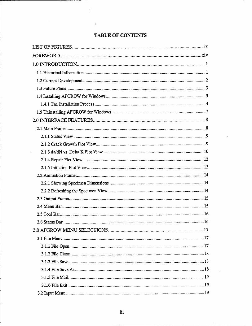
TABLE OF CONTENTS
LISTOFFIGURES ix
FOREWORD xiv
1.0 INTRODUCTION 1
1.1 Historical Information 1
1.2 Current Development 2
1.3 Future Plans 3
1.4 Installing AFGROW for Windows 3
1.4.1 The Installation Process 4
1.5 Uninstalling AFGROW for Windows 7
2.0 INTERFACE FEATURES 8
2.1 Main Frame 8
2.1.1 Status View 9
2.1.2 Crack Growth Plot View 9
2.1.3 da/dN vs. Delta K Plot View 10
2.1.4 Repair Plot View 12
2.1.5 Initiation Plot View 13
2.2 Animation Frame 14
2.2.1 Showing Specimen Dimensions 14
2.2.2 Refreshing the Specimen View 14
2.3 Output Frame 15
2.4 Menu Bar 15
2.5 Tool Bar 16
2.6 Status Bar 16
3.0 AFGROW MENU SELECTIONS 17
3.1 File Menu 17
3.1.1 Hie Open 17
3.1.2 File Close 18
3.1.3 Hie Save 18
3.1.4 File Save As 18
3.1.5 Hie Mail 19
3.1.6 Hie Exit 19
3.2 Input Menu 19
in
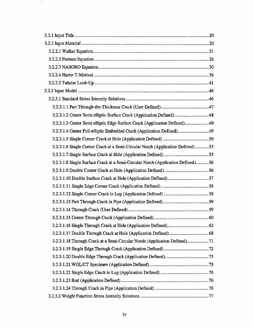
3.2.1 Input Title 20
3.2.2 Input Material 20
3.2.2.1 Walker Equation 21
3.2.2.2 Forman Equation 26
3.2.2.3 NASGRO Equation 30
3.2.2.4 Harter T-Method 36
3.2.2.5 Tabular Look-Up 41
3.2.3 Input Model 46
3.2.3.1 Standard Stress Intensity Solutions 46
3.2.3.1.1 Part Through-the-Thickness Crack (User Defined) 47
3.2.3.1.2 Center Semi-elliptic Surface Crack (Application Defined) 48
3.2.3.1.3 Center Semi-elliptic Edge Surface Crack (Application Defined) 49
3.2.3.1.4 Center Full-elliptic Embedded Crack (Application Defined) 49
3.2.3.1.5 Single Comer Crack at Hole (Application Defined) 50
3.2.3.1.6 Single Corner Crack at a Semi-Circular Notch (Application Defined) 53
3.2.3.1.7 Single Surface Crack at Hole (Application Defined) 53
3.2.3.1.8 Single Surface Crack at a Semi-Circular Notch (Application Defined) 56
3.2.3.1.9 Double Corner Crack at Hole (Application Defined) 56
3.2.3.1.10 Double Surface Crack at Hole (Application Defined) 57
3.2.3.1.11 Single Edge Corner Crack (Application Defined) 58
3.2.3.1.12 Single Corner Crack in Lug (Application Defined) 58
3.2.3.1.13 Part Through Crack in Pipe (Application Defined) 59
3.2.3.1.14 Through Crack (User Defined) 59
3.2.3.1.15 Center Through Crack (Application Defined) 60
3.2.3.1.16 Single Through Crack at Hole (Application Defined) 62
3.2.3.1.17 Double Through Crack at Hole (Application Defined) 68
3.2.3.1.18 Through Crack at a Semi-Circular Notch (Application Defined) 71
3.2.3.1.19 Single Edge Through Crack (Application Defined) 72
3.2.3.1.20 Double Edge Through Crack (Application Defined) 75
3.2.3.1.21 WOL/CT Specimen (Application Defined) 75
3.2.3.1.22 Single Edge Crack in Lug (Application Defined) 76
3.2.3.1.23 Rod (Application Defined) 76
3.2.3.1.24 Through Crack in Pipe (Application Defined) 76
3.2.3.2 Weight Function Stress Intensity Solutions 77
IV
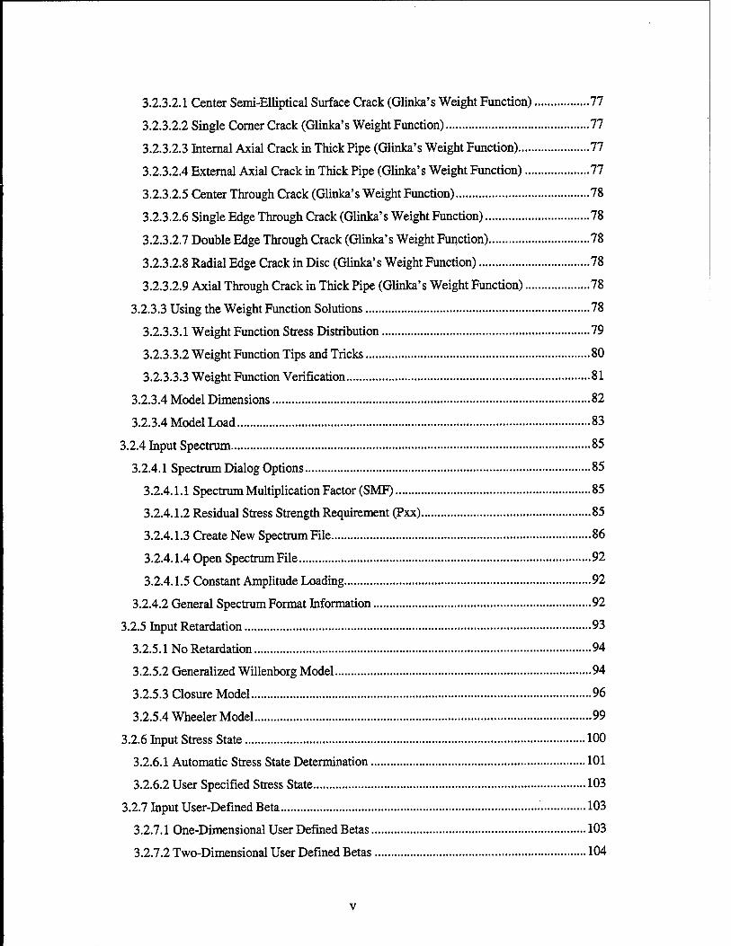
3.2.3.2.1 Center Semi-Elliptical Surface Crack (Glinka's Weight Function) 77
3.2.3.2.2 Single Corner Crack (Glinka's Weight Function) 77
3.2.3.2.3 Internal Axial Crack in Thick Pipe (Glinka's Weight Function) 77
3.2.3.2.4 External Axial Crack in Thick Pipe (Glinka's Weight Function) 77
3.2.3.2.5 Center Through Crack (Glinka's Weight Function) 78
3.2.3.2.6 Single Edge Through Crack (Glinka's Weight Function) 78
3.2.3.2.7 Double Edge Through Crack (Glinka's Weight Function) 78
3.2.3.2.8 Radial Edge Crack in Disc (Glinka's Weight Function) 78
3.2.3.2.9 Axial Through Crack in Thick Pipe (Glinka's Weight Function) 78
3.2.3.3 Using the Weight Function Solutions 78
3.2.3.3.1 Weight Function Stress Distribution 79
3.2.3.3.2 Weight Function Tips and Tricks 80
3.2.3.3.3 Weight Function Verification 81
3.2.3.4 Model Dimensions 82
3.2.3.4 Model Load 83
3.2.4 Input Spectrum 85
3.2.4.1 Spectrum Dialog Options 85
3.2.4.1.1 Spectrum Multiplication Factor (SMF) 85
3.2.4.1.2 Residual Stress Strength Requirement (Pxx) 85
3.2.4.1.3 Create New Spectrum File 86
3.2.4.1.4 Open Spectrum File 92
3.2.4.1.5 Constant Amplitude Loading 92
3.2.4.2 General Spectrum Format Information 92
3.2.5 Input Retardation 93
3.2.5.1 No Retardation 94
3.2.5.2 Generalized Willenborg Model 94
3.2.5.3 Closure Model 96
3.2.5.4 Wheeler Model 99
3.2.6 Input Stress State 100
3.2.6.1 Automatic Stress State Determination 101
3.2.6.2 User Specified Stress State 103
3.2.7 Input User-Defined Beta 103
3.2.7.1 One-Dimensional User Defined Betas 103
3.2.7.2 Two-Dimensional User Defined Betas 104

3.2.7.2.1 Four-Point User-Defined Beta Values 105
3.2.7.2.2 Linearly Interpolated User-Defined Beta Values 106
3.2.8 Input Environment 109
3.2.8.1 Modeling Environmental Crack Growth Rate Transition Behavior Ill
3.2.9 Input Beta Correction 112
3.2.9.1 Determine Beta Correction Factors Using Normalized Stresses 112
3.2.9.2 Enter Beta Correction Factors Manually 114
3.2.10 Input Residual Stresses 115
3.2.10.1 Determine Residual Stress Intensity Values Using Residual Stresses 116
3.2.10.1.1 Gaussian Integration Method 116
3.2.10.1.2 Weight Function Method 117
3.2.10.2 Enter Residual Stress Intensity Factors Manually 117
3.3 View Menu 117
3.3.1 View Standard Toolbar 118
3.3.2 View Predict Toolbar 118
3.3.3 View Status Bar 118
3.3.4 View Status 119
3.3.5 View Crack Plot 119
3.3.6 View da/dN Plot 119
3.3.7 View Repair Plot 119
3.3.8 View Initiation Plots 119
3.3.9 View Spectrum Plot 120
3.3.10 View Dimensions 120
3.3.11 View Refresh 121
3.4 Predict Menu 121
3.4.1 Predict Preferences 121
3.4.1.1 Growth Increment 122
3.4.1.2 Output Intervals 123
3.4.1.3 Output Options 124
3.4.1.4 Propagation Limits 126
3.4.1.5 Transition Options 127
3.4.2 Predict Run 128
3.4.3 Predict Stop 128
3.5 Tools Menu 128
vi

3.5.1 View Plots in Excel .128
3.5.2 Aging Aircraft Structures Database (AASD) 128
3.5.3 Run Spectrum Translator 129
3.5.4 Run Cycle Counter 130
3.6 Repair Menu 133
3.6.1 Repair Design 133
3.6.1.1 Ply Design and Lay-up 134
3.6.1.1.1 Material Properties 134
3.6.1.1.2 Ply Lay-up 135
3.6.1.1.3 Patch Type 135
3.6.1.1.4 Patch Stiffness Indicator 136
3.6.1.2 Patch Dimensions and Adhesive Properties 136
3.6.1.2.1 Sample C-Scan Image of a Repair 136
3.6.1.2.2 Adhesive Properties 137
3.6.1.2.3 Patch Dimensions 137
3.6.1.2.4 Critical SIF 137
3.6.1.3 Designed Patch Properties 138
3.6.2 Read Design Data 140
3.6.3 Repair/No Repair 140
3.6.4 Delete Repair 140
3.7 Initiation Menu 140
3.7.1 Strain-Life Initiation Methodology 141
3.7.1.1 Neuber's Rule 142
3.7.1.2 Smith-Watson-Topper Equivalent Strain 142
3.7.1.3 Fatigue Notch Factor 143
3.7.2 Initiation Parameters 143
3.7.2.1 Model/Material Data 144
3.7.2.2 Cyclic Stress-Strain / Strain-Life Equation 144
3.7.3 User-Defined Cyclic Stress-Strain / Strain-Life Data 146
3.7.3.1 Cyclic Stress-Strain Data 146
3.7.3.2 Strain-Life Data 147
3.7.4 Initiation/No Initiation 148
3.8 Window Menu 148
3.8.1 Window Cascade 149
vn

3.8.2 Window Tile 150
3.9 Help Menu 151
3.9.1 Help Topics 151
3.9.2 About AFGROW 152
4.0 ENGLISH AND METRIC UNITS 153
5.0 COMPONENT OBJECT MODEL SERVER 154
6.0 TUTORIAL 156
6.1 Problem Definition 156
6.2 Entering Data in AFGROW 157
6.2.1 Input Title 157
6.2.2 Input Material 158
6.2.3 Input Model 159
6.2.4 Input Spectrum 160
6.2.5 Input Retardation 162
6.2.6 Stress State 163
6.2.7 Residual Stresses 163
6.2.8 Predict Preferences 164
6.3 AFGROW Output 165
Vlll
LIST OF FIGURES
Figure 1: AFGROW Self-Extracting Setup Dialog 4
Figure 2: AFGROW Splash Screen 4
Figure 3: AFGROW Installation Directory 5
Figure 4: AFGROW Program Folder Name 5
Figure 5: Final Installation Dialog 6
Figure 6: Notification of Successful Program Registration 6
Figure 7: Add/Remove Programs Dialog 7
Figure 8: AFGROW Windows Graphical User Interface 8
Figure 9: Mainframe Functions 8
Figure 10: Status View 9
Figure 11: Crack Growth Plot View 10
Figure 12: Rebar Tool 10
Figure 13: da/dN vs. Delta K Plot View 11
Figure 14: Repair Plot View 12
Figure 15: Initiation Plot View 13
Figure 16: Animation Frame 14
Figure 17: Output Frame 15
Figure 18: Menu Bar 15
Figure 19: Tool Bar 16
Figure 20: Status Bar 16
Figure 21: File Menu »17
Figure 22: File Open Dialog 17
Figure 23: File Save As Dialog 18
Figure 24: Input Menu 19
Figure 25: Input Title Dialog 20
Figure 26: Input Material Dialog 20
Figure 27: Walker Equation Dialog 21
Figure 28: Walker Equation. 21
Figure 29: Closure Factor vs. Stress Ratio 22
IX
Figure 30: Using the Walker Equation with Multiple Segments 23
Figure 31: Discontinuous Crack Growth Rate Curves 24
Figure 32: Forman Equation Dialog 26
Figure 33: Forman Equation 26
Figure 34: Forman Equation Material Property Dialog 27
Figure 35: NASGRO Equation Dialog 30
Figure 36: NASGRO Equation Constants 32
Figure 37: Opening the NASGRO Material Database 33
Figure 38: Material Database Browser 33
Figure 39: Database Material Selection 34
Figure 40: Harter T-Method Dialog 36
Figure 41: Harter T-Method Crack Growth Rate Shifting as a Function of R 37
Figure 42: Tabular Look-Up Dialog 41
Figure 43: Tabular Look-Up Default Material Data 42
Figure 44: Tabular Look-Up Copy Choices 42
Figure 45: Tabular Look-Up Paste Choices 43
Figure 46: Excel Spreadsheet Example for Crack Growth Rate Data 43
Figure 47: Input Model Dialog 46
Figure 48: Angle Used in Newman and Raju Solutions 47
Figure 49: Sample Beta Solutions for an Offset Hole, B > W/2 52
Figure 50: Straight Through-the-Thickness Cracks 62
Figure 51: Oblique Through-the-Thickness Cracks 62
Figure 52: Oblique Through-the-Thickness Crack Geometry 65
Figure 53: In-Plane Bending Constraint Option for the Edge Cracked Plate 72
Figure 54: Weight Function Stress Distribution Dialog 79
Figure 55: Comparison Between Weight Function and Standard Solutions 80
Figure 56: Center Crack Under Uniform Tensile Loading 81
Figure 57: Edge Crack Under an Out-of-Plane Bending Load 82
Figure 58: Model Dimensions Dialog 82
Figure 59: Model Load Dialog 83
Figure 60: Input Spectrum Dialog 85
Figure 61: Spectram Information Dialog 86
Figure 62: Spectrum Type Dialog 87
Figure 63: Sub-Spectra Dialog 88
Figure 64: Stress Level Dialog 89
Figure 65: Stress Levels 90
Figure 66: Spectrum Wizard Finish Dialog 91
Figure 67: Constant Amplitude Spectrum Dialog 92
Figure 68: Retardation Model Dialog 93
Figure 69: Willenborg Retardation Parameter Dialog 95
Figure 70: Closure Retardation Model Dialog 96
Figure 71: AFGROW Closure Model 97
Figure 72: Wheeler Model Dialog 99
Figure 73: Stress State Dialog 100
Figure 74: Stress State Information 102
Figure 75: Through Crack User-Defined Beta Table Dialog 104
Figure 76: 2-D User Input Beta Dialog 105
Figure 77: Four-Point Beta Interpolation Dialog 106
Figure 78: Linear Interpolation Dialog 107
Figure 79: Environment Dialog 109
Figure 80: Environmental Depiction in the Animation Frame 109
Figure 81: Environmental File Open Dialog 110
Figure 82: AFGROW Environmental Rate Transition Model Ill
Figure 83: Beta Correction Factor Dialog 112
Figure 84: Slope Between Input Data Points 113
Figure 85: Point Load Stress Intensity Solution 113
Figure 86: Residual Stress Dialog 115
Figure 87: View Menu 117
Figure 88: Standard Toolbar 118
Figure 89: Predict Toolbar 118
Figure 90: Spectrum Plot 120
Figure 91: Specimen Dimensions 120
XI
Figure 92: Predict Menu 121
Figure 93: Preference Categories 121
Figure 94: Saving and Restoring Preferences 121
Figure 95: Growth Increment Dialog 122
Figure 96: Output Interval Dialog 123
Figure 97: Output Options Dialog 124
Figure 98: Sample Output Data 125
Figure 99: Propagation Limits Dialog 126
Figure 100: Transition Options Dialog 127
Figure 102: Dialog Box to View Plots in Excel 128
Figure 103: Aging Aircraft Structures Database 129
Figure 104: Spectrum Translator 130
Figure 105: Cycle Definition 130
Figure 106: Sample Uncounted Stress Sequence 131
Figure 107: Cycle Counting Software Interface 131
Figure 108: Ply Design and Lay-up Dialog 134
Figure 109: Patch Dimensions and Adhesive Properties Dialog 136
Figure 110: Patch Dimensions and Adhesive Properties Dialog 138
Figure 111: Repair Beta Correction vs. Crack length 139
Figure 112: Specimen Cross Section View with a Bonded Repair 139
Figure 113: Opening a Repair Design File 140
Figure 113: Neuber's Rule 142
Figure 114: Initiation Parameters Dialog 143
Figure 115: Cyclic Stress-Strain / Strain-Life Equation Dialog 144
Figure 116: Using Default Initiation Parameters for Common Materials 145
Figure 117: Options for User Defined Initiation Data 146
Figure 118: Options for Stress-Strain and Strain-Life Input Data 146
Figure 119: User-Defined Cyclic Stress-Strain Data 146
Figure 121: Stable Hysteresis Curves 147
Figure 121: User-Defined Strain-Life Data 147
Figure 122: Window Menu 148
Xll

Figure 123: Cascade Window View 149
Figure 124: Tile Window View 150
Figure 125: AFGROW Help Topics 151
Figure 126: Help About AFGROW 152
Figure 127: Switching Between English and Metric Units 153
Figure 128: Microsoft Excel Macro Using AFGROW 154
Figure 129: Sample Problem Geometry 156
xiu

FOREWORD
This report summarizes over 15 years of work to develop a user-friendly structural life prediction program.
The author would like to thank the U.S. Navy and Air Force for funding this effort over the last 12 years and all of the people who have provided moral support and encouragement over the years. Thanks also to Srinivas Krishnan, Alexander Litvinov, and Deviprasad Taluk for the top-notch software and finite element modeling support, which made AFGROW the best life prediction program available.
Special thanks to my wife, Cheri, for her understanding and patience during the long nights and weekends I devoted to AFGROW.
xiv

1.0 INTRODUCTION
1.1 Historical Information
AFGROW's history traces back to a crack growth life prediction program (ASDGRO), which was written in BASIC for IBM-PCs by Mr. Ed Davidson at ASD/ENSF in the early-mid 1980's. In 1985, ASDGRO was used as the basis for crack growth analysis for the Sikorsky H-53 Helicopter under contract to Warner-Robins ALC. The program was modified to utilize very large load spectra, approximate stress intensity solutions for cracks in arbitrary stress fields, and use a tabular crack growth rate relationship based on the Walker equation on a point-by-point basis (Harter T-Method). The point loaded crack solution from the Tada, Paris, and Irwin Stress Intensity Factor Handbook was originally used to determine K (for arbitrary stress fields) by integration over the crack length using the unflawed stress distribution independently for each crack dimension. After discussions with Dr. Jack Lincoln (ASD/ENSF), a new method was developed by Mr. Frank Grimsley (AFWAL/FIBEC) to determine stress intensity, which used a 2-D Gaussian integration scheme with Richardson Extrapolation which was optimized by Dr. George Sendeckyj (AFWAL/FIBEC). The resulting program was named MODGRO since it was a modified version of ASDGRO.
In 1987, James Harter came to work for the Air Force Wright Aeronautical Laboratories (AFWAL/FIBEC) and rewrote MODGRO, Version l.X (still in BASIC for PC DOS). Over the next 2 years, a tabular crack growth rate database was added. Decreasing- increasing crack growth rate tests were performed to obtain data below 1.0E-08 inches/cycle for 7075-T651 Aluminum and 4340 Steel. During that period, MODGRO, Version l.X [1] included part-through flaw solutions from Newman and Raju, and standard closed-form solutions for symmetrical through-cracks (center, single edge, and double edge cracks). These solutions could also be modified for arbitrary stress fields using a Gaussian integration method with a stress distribution defined by the ratio of the unflawed stress field of interest divided by the unflawed stress field for the baseline geometry. The error in this method, of course, increases with crack length, but error in life is minor since the majority of life is consumed while the crack lengths are relatively short.
In 1989, MODGRO, Version 2.0 was rewritten in Turbo Pascal for PC-DOS as a move to a more structured computer language. At that time, Dr. George Sendeckyj provided MUCH assistance in debugging and optimizing the arithmetic operations. George was also learning the C language and was practicing by translating the BASIC code to Structured BASIC and then C at the same time I was coding it in Turbo Pascal. Runtime comparisons were made in the spirit of friendly competition. Actually, George's C version of MODGRO, Version 1.0 was faster. George was the first to have written a version of MODGRO in the C language. Additions to version 2.0 of the code included a plasticity based closure model, which was based on work by Erdogan, Irwin, Elber, M. Creager, and Sunder [2, 3, and 4]. The model is a variable amplitude closure model and more detail is contained in this report. There is also credit due to Mitch Kaplan [5] because of his good suggestion to only recalculate the beta (or alpha) values at user

defined crack growth increments. It was decided to simply use the user-input value for the Vroman integration percentage, which is normally used when analyzing blocked spectra. A real-time crack length plotting capability was also added to the program. The code was totally changed in the process, but the name MODGRO remained.
From 1990-1993 the code changed very little (still released in Turbo Pascal). Small changes/repairs were made based on errors that were discovered. The code was used to help manage the flight test program for the X-29. During high angle-of-attack maneuvers, the vertical tail experienced severe buffeting. MODGRO, Version 2.0 was used by NASA/Dryden to estimate the vertical tail life from actual flight test data collected for each flight. The use of the code allowed the Program Managers to assess the effect of various flight maneuvers on the vertical tail, and in some cases, flights were re-arranged to maximize the amount of flight data and minimize tail damage accumulation.
In 1993, the Navy was interested in using MODGRO to assist in a program to assess the effect of certain (classified) environments on the damage tolerance of aircraft. The Navy wanted to build a user-friendly code to be used in the program and initiated an agreement with WL/FIBEC to develop a state-of-the-art user interface with the added capability to perform life analysis under adverse environments. This effort required additional manpower for software development and baseline crack growth testing. On-site contract support was used to meet this requirement. Work began at that time to convert the MODGRO, Version 3.0 to the C language for UMX to provide performance and portability to several UMX Workstations [6]. The workstation platform was chosen to provide additional computational power for MODGRO.
In 1994, a research contract with Analytical Services and Materials was established to provide support for the Navy effort and assist in future research and development requirements of WL/FIBEC. This was when the current UNIX interface was bom. In July 1994, a presentation of the results for the Navy project was given to the Navy sponsor and WL/FEBE management. After the presentation, the WL/FEBE Branch Chief (Mr. Jerome Pearson) requested that the code be renamed AFGROW, Version 3.0. Work on the Windows 95 version of AFGROW was started in October of 1996.
1.2 Current Development
Since work on the Windows95 version of AFGROW commenced in 1996, it has become the main version for new capabilities and enhancements. A composite bonded repair crack growth analysis capability was added during 1996-97. The bonded repair capability was based entirely on work by Dr. Mohan Ratwani [7]. In addition, a strain-life based crack initiation analysis capability was added. The strain-life initiation analysis capability was taken from APES, Inc. [8]. During reorganizations at Wright-Patterson AFB, it was decided that AFGROW would not receive further research and development funds. As a result, the on-site software development support provided by Analytical Services and Materials was reduced significantly. Since the Windows95 version of AFGROW had become most widely used, it was decided to discontinue the UNIX support. Recent advances in windows hardware capability has made it possible for AFGROW to equal
and even surpass the performance capabilities of many UNIX systems. The Air Force organization responsible for AFGROW development was changed from WL/FEBEC to AFRL/VASE during the most recent reorganization in 1998.
In late 1997 and early 1998, the U.S. Navy provided AFGROW funding to support a fleet tracking database development effort (FLEETLIFE) for the AV-8 Harrier. It was decided to add the Microsoft Component Object Model (COM) server technology [9] to AFGROW. This capability allows AFGROW to be used by any Windows software. Since the FLEETLIFE code was being written for the Windows platform, this provided an efficient means for the fleet tracking database to use AFGROW for structural life analyses.
The AFGROW user base continued to grow dramatically in 1998. Air Force Air Logistic Center (ALC) use and strong support for the code was greatly responsible for additional funding, provided in late 1998, for multiple crack and time dependent analysis capabilities. The Air Force Aging Aircraft Office (ASC/SMS) provided these funds. As a result of this funding and requests for UNIX support, the UNIX version of AFGROW will be upgraded to match the capabilities of the Windows version.
An experimental Power Macintosh version of AFGROW was released in late 1998 for evaluation purposes.
1.3 Future Plans
AFGROW will undergo a major overhaul in 1999 to facilitate the new multiple crack and time dependence capabilities. The multiple crack capability will allow AFGROW to analyze cases with more than one crack growing from a row of fastener holes. Stress intensity factor solutions are available for many of these cases [10, 11], but few life analysis codes have included this capability to date. The time dependent crack growth capability will provide a means of including crack growth as a function of time in addition to the standard cyclic dependence that is the default in most crack growth programs.
One of the biggest challenges to the multiple crack analysis capability is the design of the user interface. AFGROW will include a drag and drop design interface for the multiple crack capability.
As always, the developers of AFGROW will continue to listen to users comments and suggestions to improve the code.
1.4 Installing AFGROW for Windows *e>
AFGROW, for Windows 95/98/NT4, is available for download in two forms. The first is a single self-extracting executable file that may be executed on a users PC. This file is approximately 3.5 to 4 MB in size. In case users find the single file too large to download (problem with an internet connection, etc.), AFGROW is also available in three floppy

disk images. Each file is less than 1.44MB and is "zipped" using a shareware version of the program, Winzip (available at www.winzip.com). The files should be "unzipped" to three floppy disks. The first disk contains the setup program and users will be prompted to insert disk 2 and 3 as required during the installation process.
1.4.1 The Installation Process
AFGROW uses the Install Shield© program to generate the installation program required to copy and register the required program files to an individual PC. If the single file method is used, the dialog shown in Figure 1 appears:
|WinZip Self-Extiactoi [A_V3-9~1.EXE] Qj
AFGROW ! Selup Vr|
WinZip® Self-Extraclor © Nico Mak Computing, Ina httpiMw*
Cancel
'••:■•. About
w. vwizip.com
Figure 1: AFGROW Self-Extracting Setup Dialog
The installation procedure is started when the user selects the setup button in the above dialog box (Figure 1).
Once the installation has been started (using the single or multiple file methods), the following dialog (Figure 2) is displayed:
Welcome
-"""■" ■•.-. . > -*• ■ - —■
*s £5~„
^W^^'M^MSmMw^ßS^M
xgack |rjigxt> j Caricej |
Figure 2: AFGROW Splash Screen
A blue background also appears with logos for AFRIWASE and Analytical Services and Materials (AS&M). This splash screen is also used each time AFGROW is opened. The installation process proceeds as the user selects next (or back) on each dialog.
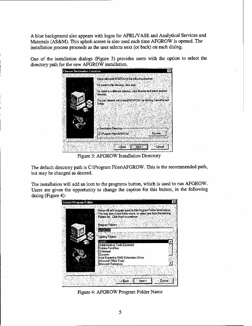
One of the installation dialogs (Figure 3) provides users with the option to select the directory path for the new AFGROW installation.
Choose Destination Location
Setup will install AFGROW in the following directory.
To install to this directory, click Next.
?;tp install to aaK&enJditectory.-clicfeBr^
S'ou can choose not to install AFGF30V/> by cricking Cancel to edit Setup
■ Destination Directory ;
C:\Ptogiam FJesUFGROW ::Browse.i.:
"|Back ■■■■j|t.. /Next*/ .Cancel
Figure 3: AFGROW Installation Directory
The default directory path is C:\Program Files\AFGROW. This is the recommended path, but may be changed as desired.
The installation will add an icon to the programs button, which is used to run AFGROW. Users are given the opportunity to change the caption for this button, in the following dialog (Figure 4):
Select Piogiam Foldet
'Setup Wffl add program!^ rai may type a new folder name; or^^sefect one from the e«isting- Foldetsfct Click Next to continue.
Program Folders:
Existing Folders
Administrative Tools (Common) Delrina FormFlow Diskeeper Dynamix Intel Streaming SIMD Extensions Driver Microsoft Office Tools Microsoft Reference _3
<Back ) Next> | Cancel j
Figure 4: AFGROW Program Folder Name
It is expected that the name AFGROW will be used, but users have the option to customize the name. For example, users can include version number in the name if desired. However, do NOT attempt to install multiple versions of AFGROW since that will cause problems with the Component Object Model (COM) capabilities (see section 5.0).
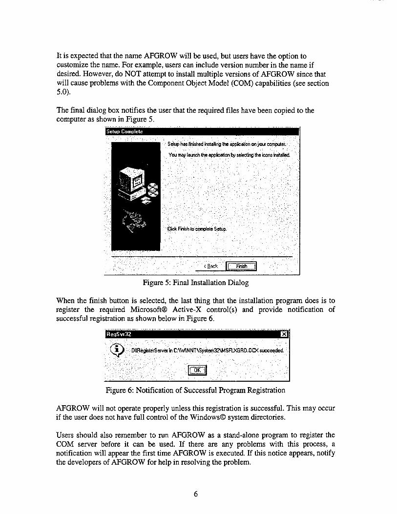
The final dialog box notifies the user that the required files have been copied to the computer as shown in Figure 5.
1 Setup Complete [
;.■;::•
V .
Söup has finished installing the application on your computer.'
You may launch the application by selecting the icons installed
Qick Finish to complete Setup. ■'■■■'.:
<Back |F Finish sj
Figure 5: Final Installation Dialog
When the finish button is selected, the last thing that the installation program does is to register the required Microsoft® Active-X control(s) and provide notification of successful registration as shown below in Figure 6.
|RegSvr32
;<S> : DBRegisterServei in C:\WINNT\System32\MSFLXGRD.0CX succeeded
LSKJ
Figure 6: Notification of Successful Program Registration
AFGROW will not operate properly unless this registration is successful. This may occur if the user does not have full control of the Windows© system directories.
Users should also remember to run AFGROW as a stand-alone program to register the COM server before it can be used. If there are any problems with this process, a notification will appear the first time AFGROW is executed. If this notice appears, notify the developers of AFGROW for help in resolving the problem.
1.5 Uninstalling AFGROW for Windows
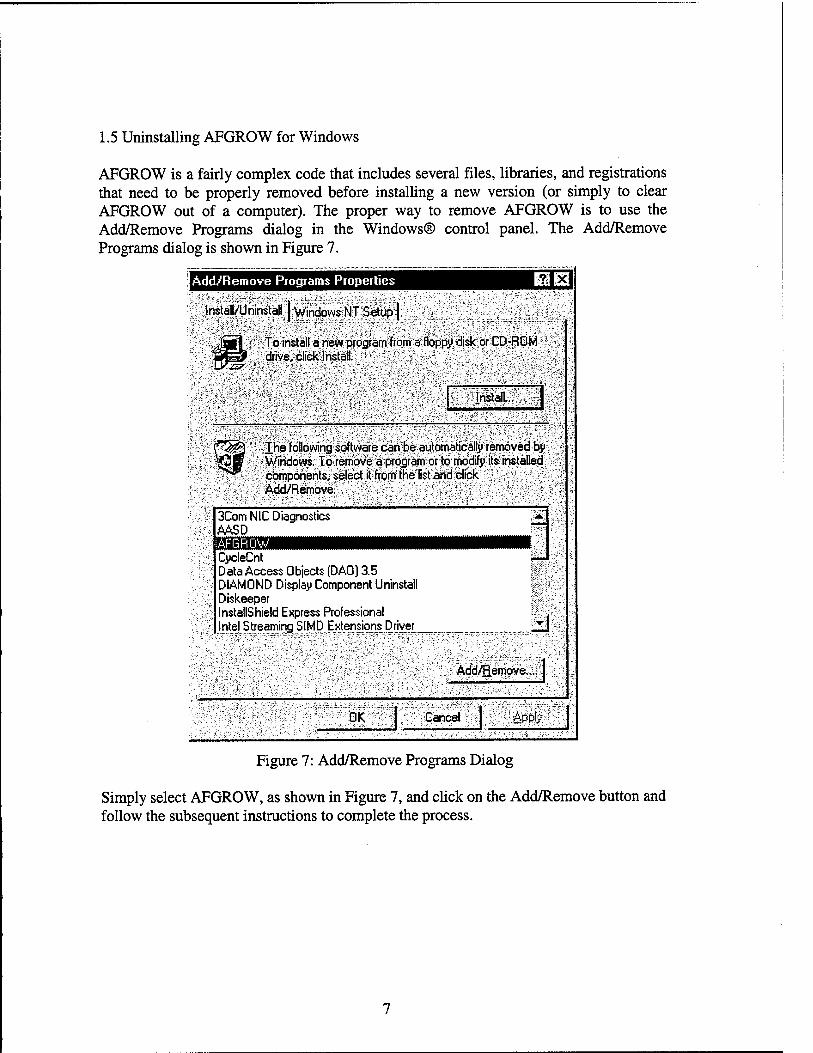
AFGROW is a fairly complex code that includes several files, libraries, and registrations that need to be properly removed before installing a new version (or simply to clear AFGROW out of a computer). The proper way to remove AFGROW is to use the Add/Remove Programs dialog in the Windows® control panel. The Add/Remove Programs dialog is shown in Figure 7.
Add/Remove Programs Properlies
InstallAJninstall Windows NT Setup
RfllSl
To install a new program from a floppy disk or CD-ROM drive, click Install.
Install...
Ihe following software can be automatical!!» removed by Windows. To remove a program or to modify its installed components, select it from the list and click Add/Remove.
3Com NIC Diagnostics AASD IAFGROW CycleCnt Data Access Objects (DAO) 3.5 DIAMOND Display Component Uninstall Diskeeper InstallShield Express Professional Intel Streaming SIMP Extensions Driver
Ädd/Remove... j
OK" Cancel Apply'
Figure 7: Add/Remove Programs Dialog
Simply select AFGROW, as shown in Figure 7, and click on the Add/Remove button and follow the subsequent instructions to complete the process.
2.0 INTERFACE FEATURES
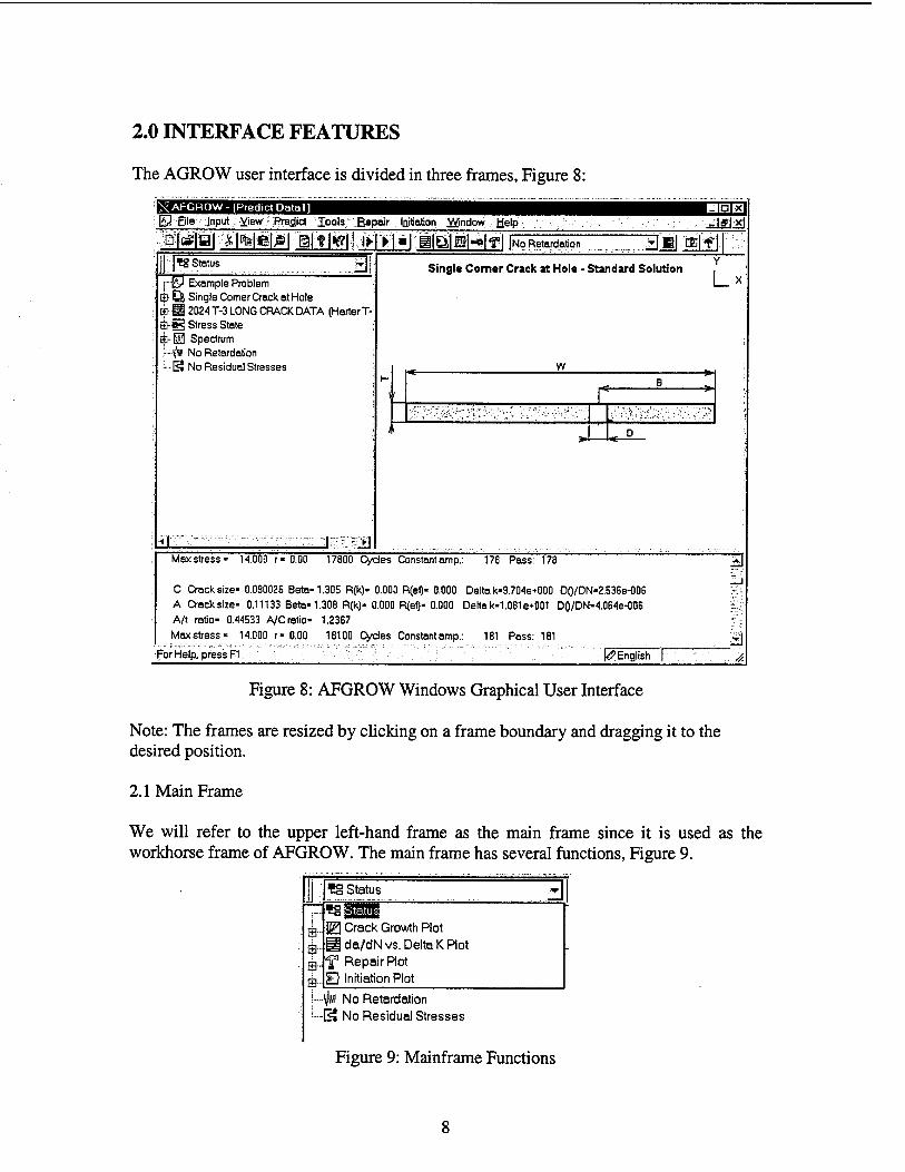
The AGROW user interface is divided in three frames, Figure 8:
X AFGROW- [Predict Datal] CA 5le Input Vjew Predict Iools -Repair ■ Initiation .Mtfndow Melp jff]*] D|cg|y| ^NfelPl al?l*?l jf ► JEJ MÖ B'i'f |NO Retardation "BMMil
*8 Status ~3\ fei Example Problem
<$ Q Single Comer Crack at Hole il 2024 T-3 LONG CRACK DATA (Harter T- i-g Stress State ia-0 Spectrum I # No Retardation '< S No Residual Stresses
Single Corner Crack at Hole - Standard Solution
J«:=T±J
L_x
_ w
V B
-'•■'• '■ ,'\~'" '"i"'' ' ■ ",' '■■' '~ :■ '■*'■■ V- ^'^.Vfr:];'^.;''"': ^'J^''u!':':'""'. .'-1"'.
i > —S-
Maxstress- 14.000 r-0.00 17800 Cydes Constant amp.: 178 Pass: 178
C Crack size- 0.090026 Beta-1.305 R(k)- 0.000 R(ef)- 0.000 Delta k-9.704e+000 D0/DN-2.53Be-O06
A Crack size- 0.11133 Beta-1.308 R(k)- 0.000 R(ef)- 0.000 Delta k-1.081 e+001 DO/DN-4.064e-006 A/t ratio- 0.44533 A/C ratio- 1.23B7
Max stress- 14.000 r-0.00 18100 Cycles Constant amp.: 181 Pass: 181
For Help, press F1 ^English
"3
Figure 8: AFGROW Windows Graphical User Interface
Note: The frames are resized by clicking on a frame boundary and dragging it to the desired position.
2.1 Main Frame
We will refer to the upper left-hand frame as the main frame since it is used as the workhorse frame of AFGROW. The main frame has several functions, Figure 9.
j0 Crack Growth Plot da/dN vs. Delta K Plot
f3 Repair Rot SO Initiation Plot
j # No Retardation ! S No Residual Stresses
Figure 9: Mainframe Functions
The desired view may be selected using the pull-down list as shown in Figure 9 above and selecting the view of interest.
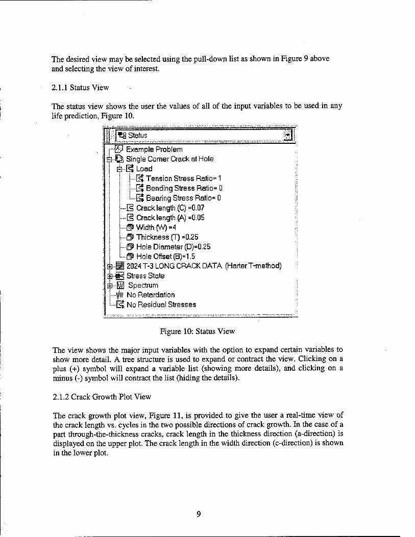
2.1.1 Status View
The status view shows the user the values of all of the input variables to be used in any life prediction, Figure 10.
18 Status
i m
Example Problem Single Comer Crack at Hole HjLoad
■-EJ Tension Stress Ratio= 1 ■•■•EK Bending Stress Ratio= 0 ■~E^ Bearing Stress Ratio= 0
E Crack length (C) =0.07 g Crack length (A) =0.05 m Width (W) =4 & Thickness (T) =0.25 fiP Hole Diameter (D)=0.25 & Hole Offset (B)=1.5 2024 T-3 LONG CRACK DATA (Harter T-method) Stress State Spectrum No Retardation No Residual Stresses
Figure 10: Status View
The view shows the major input variables with the option to expand certain variables to show more detail. A tree structure is used to expand or contract the view. Clicking on a plus (+) symbol will expand a variable list (showing more details), and clicking on a minus (-) symbol will contract the list (hiding the details).
2.1.2 Crack Growth Plot View
The crack growth plot view, Figure 11, is provided to give the user a real-time view of the crack length vs. cycles in the two possible directions of crack growth. In the case of a part through-the-thickness cracks, crack length in the thickness direction (a-direction) is displayed on the upper plot. The crack length in the width direction (c-direction) is shown in the lower plot.

110 Crack Growth Plot urn Wb &
0.226 A
0.169
0.113
0.0565
0
0.72? C
0.546
0.364
0.182
0
Crack Length vs. Cycles
2otes 40250
20feS 40250
Line numb« one
Figure 11: Crack Growth Plot View
There are several features incorporated in this view. First, we use the Microsoft rebar tool, Figure 12, to save window space and provide several useful tools.
C| D| 0 Figure 12: Rebar Tool
The rebar tool slides to the. right and left by clicking on the handle (2 vertical bars), holding the left mouse button down, and dragging the tool to the left or right.
The first tool (left most button) is the overlay tool. Clicking on this button causes the crack length plots for each prediction (up to the last eight runs) to appear on the same plot for comparison purposes.
The second tool (middle button) is the property tool. It allows the user to select various plot properties such as the plot legend, black and white plots, and reverse plotting. Reverse plotting reverses the x-axis and shows the number of cycles remaining until failure.
The third tool (right most button) is the erase tool. This tool simply erases all plots from the plot view.
2.1.3 da/dN vs. Delta K Plot View
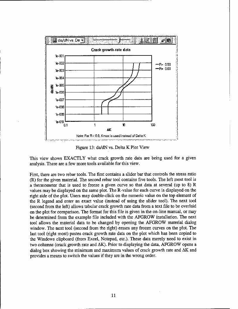
As may be suspected, this view shows the crack growth rate versus AK data for the given material and crack growth rate method being used (Forman, Walker, Tabular, etc.). Data for negative R values may be handled differently for each crack growth rate model. This information is displayed at the bottom of the plot, Figure 13.
10
I da/dN vs. Deff IK Crack growth-rate data
Ml
Note: For R < 0.0, Kmax is used instead of Delta K
Figure 13: da/dN vs. Delta K Plot View
This view shows EXACTLY what crack growth rate data are being used for a given analysis. There are a few more tools available for this view.
First, there are two rebar tools. The first contains a slider bar that controls the stress ratio (R) for the given material. The second rebar tool contains five tools. The left most tool is a thermometer that is used to freeze a given curve so that data at several (up to 8) R values may be displayed on the same plot. The R-value for each curve is displayed on the right side of the plot. Users may double-click on the numeric value on the top element of the R legend and enter an exact value (instead of using the slider tool). The next tool (second from the left) allows tabular crack growth rate data from a text file to be overlaid on the plot for comparison. The format for this file is given in the on-line manual, or may be determined from the example file included with the AFGROW installation. The next tool allows the material data to be changed by opening the AFGROW material dialog window. The next tool (second from the right) erases any frozen curves on the plot. The last tool (right most) pastes crack growth rate data on the plot which has been copied to the Windows clipboard (from Excel, Notepad, etc.). These data merely need to exist in two columns (crack growth rate and AK). Prior to displaying the data, AFGROW opens a dialog box showing the minimum and maximum values of crack growth rate and AK and provides a means to switch the values if they are in the wrong order.
11
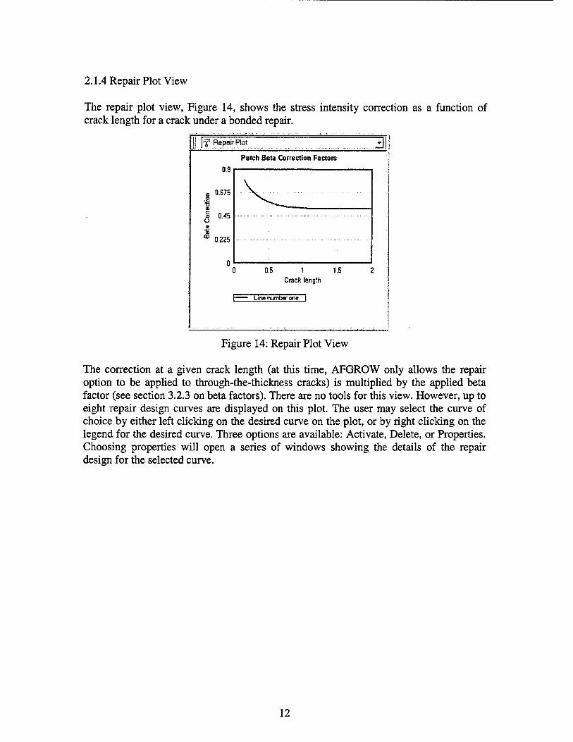
2.1.4 Repair Plot View
The repair plot view, Figure 14, shows the stress intensity correction as a function of crack length for a crack under a bonded repair.
•f" Repair Rot ^r
Patch Beta Correction Factors
c 0.675 o
■■c
o 0.45
\^ :
CO
& 0.225
0 0.5 1 1.5
Crack length
Line number one
Figure 14: Repair Plot View
The correction at a given crack length (at this time, AFGROW only allows the repair option to be applied to through-the-thickness cracks) is multiplied by the applied beta factor (see section 3.2.3 on beta factors). There are no tools for this view. However, up to eight repair design curves are displayed on this plot. The user may select the curve of choice by either left clicking on the desired curve on the plot, or by right clicking on the legend for the desired curve. Three options are available: Activate, Delete, or Properties. Choosing properties will open a series of windows showing the details of the repair design for the selected curve.
12

2.1.5 Initiation Plot View
AFGROW uses a strain-life based crack initiation analysis method to predict crack initiation life. The initiation plot view, Figure 8, displays the cyclic stress strain or the strain-life data to be used for a given analysis.
]SE} Initiation Plot u i mMMMm Cyclic stress-strain curve
0.005 0.01 0.015 Strain
Stress-Strain Eq.
0.02
Figure 15: Initiation Plot View
The cyclic stress-strain plot includes a line representing the current Young's modulus to allow the user to verify that the appropriate modulus value is being used for the input cyclic data. If it is not correct, this must be changed in the appropriate material data dialog box.
There are five tools available for the initiation plot view. The first (left most) activates the cyclic stress-strain plot. The cyclic stress-strain curve is the locus of the endpoints of stable hysteresis loops for the given material. The next tool (second from the left) activates the strain-life plot for the given material. The strain-life data is usually obtained for small round bar specimens, but is only applicable for the given lives to a specified initial crack size. The next tool allows tabular cyclic stress-strain or strain-life data from a text file to be overlaid on the plot for comparison. The format for these files is given in the on-line manual, or may be determined from the example files included with the AFGROW installation. The next tool (second from the right) erases any overlaid data from the plot. The last tool (right most) pastes cyclic stress-strain or strain-life data on the plot, which has been copied to the Windows clipboard (from Excel, Notepad, etc.). These data merely need to exist in two columns (stress and strain or strain and life). Prior to displaying the data, AFGROW opens a dialog box showing the minimum and maximum values for each value and provides a means to switch the values if they are in the wrong order.
13
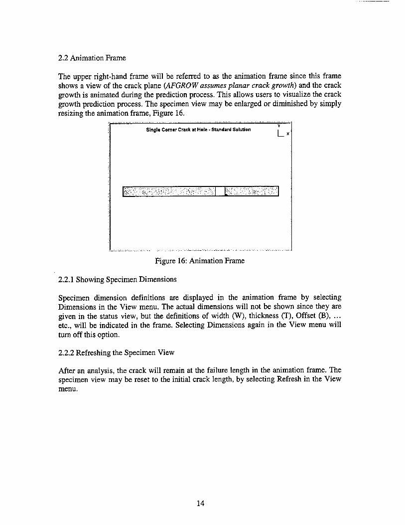
2.2 Animation Frame
The upper right-hand frame will be referred to as the animation frame since this frame shows a view of the crack plane (AFGROW assumes planar crack growth) and the crack growth is animated during the prediction process. This allows users to visualize the crack growth prediction process. The specimen view may be enlarged or diminished by simply resizing the animation frame, Figure 16.
Single Corner Crack at Hole - Standard Solution X
.?-;•' :,\ '!,- '* '■ *> - '' - >: !
Figure 16: Animation Frame
2.2.1 Showing Specimen Dimensions
Specimen dimension definitions are displayed in the animation frame by selecting Dimensions in the View menu. The actual dimensions will not be shown since they are given in the status view, but the definitions of width (W), thickness (T), Offset (B), ... etc., will be indicated in the frame. Selecting Dimensions again in the View menu will turn off this option.
2.2.2 Refreshing the Specimen View
After an analysis, the crack will remain at the failure length in the animation frame. The specimen view may be reset to the initial crack length, by selecting Refresh in the View menu.
14
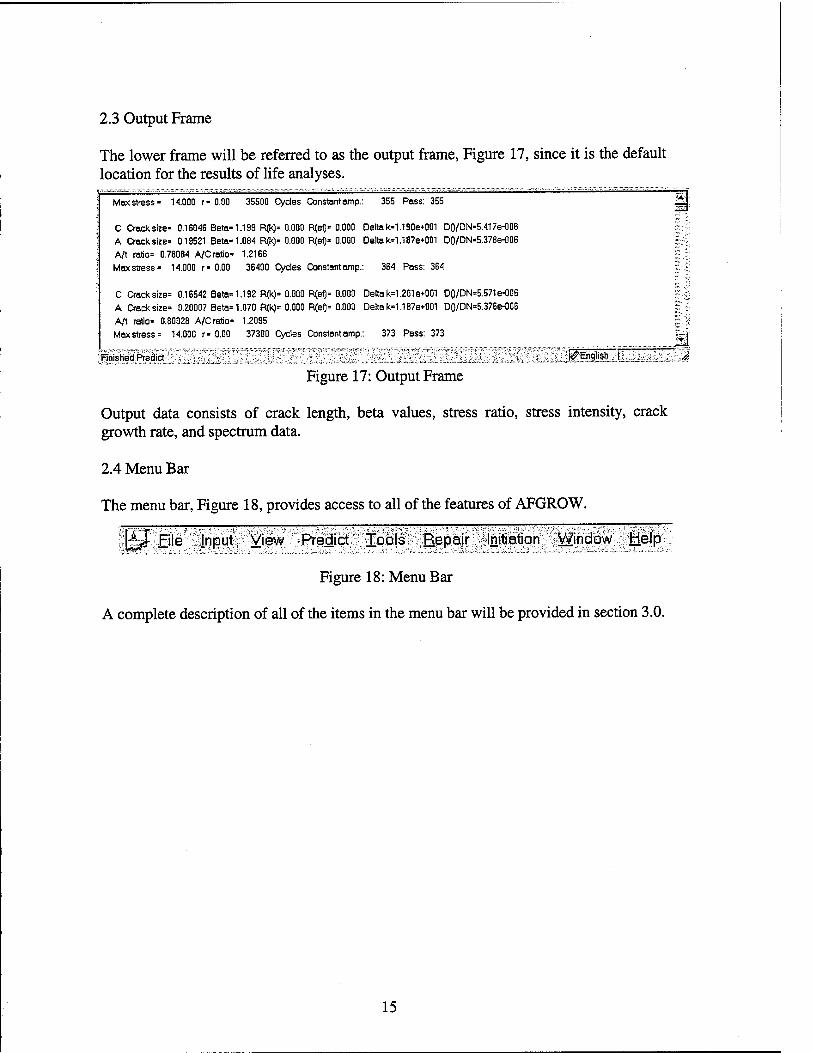
2.3 Output Frame
The lower frame will be referred to as the output frame, Figure 17, since it is the default location for the results of life analyses.
Mox stress- 14.000 r- 0.00 35500 Cycles Constant amp.: 355 Pass: 355 .23;
C Crack size- 0.16046 Beta-1.199 R(k)-0.000 R(ef)-0.000 Delta k-1.190e*001 D0/DN-5.417e-006 |:|
A Crack size- 0.19521 Beta-1.084 R(k)- 0.000 R(ef)- 0.000 Delta k-1.187e+001 D0/DN=5.378e-006 f~k
A/t ratio- 0.78084 A/C ratio- 1.2166 £■.;; Max stress- 14.000 r-0.00 36400 Cycles Constant amp.: 364 Pass: 364 5 |
C &ack size- 0.16542 Beta-1.192 R(k)= 0.000 R(ef)= 0.000 Delta k=1.201 e*001 DO/DN=5.571e-006 |;|
A Crack size- 0.20007 Beta-1.070 R(k)= 0.000 R(ef)= 0.000 Delta k=1.187e*001 D0/DN=5.376e-006 |j
A/t ratio- 0.80028 A/C ratio- 1.2095 || Max stress- 14.000 r-0.00 37300 Cycles Constant amp.: 373 Pass: 373 iWr
Finished Predict " ~ * ' ..'.,.... . .' . . h?.En9|?h_ J ._ _ -<*
Figure 17: Output Frame
Output data consists of crack length, beta values, stress ratio, stress intensity, crack growth rate, and spectrum data.
2.4 Menu Bar
The menu bar, Figure 18, provides access to all of the features of AFGROW.
\^fl File Input View Predict Tools Ftepair Initiation Window Help
Figure 18: Menu Bar
A complete description of all of the items in the menu bar will be provided in section 3.0.
15
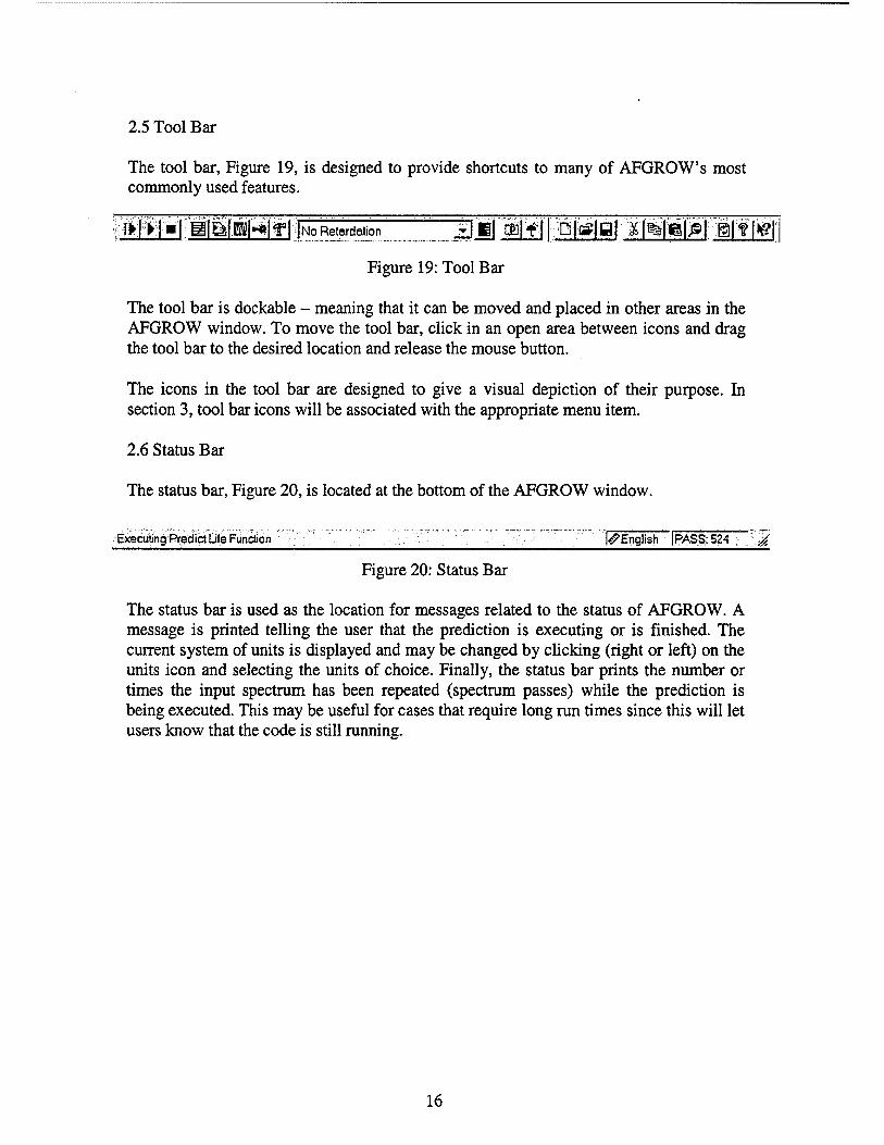
2.5 Tool Bar
The tool bar, Figure 19, is designed to provide shortcuts to many of AFGROW's most commonly used features.
I* *>: ••■ BlliNlf IjNo Retardation JL] El Wf! ^Mö] ffiftfelffl jffjiff
Figure 19: Tool Bar
The tool bar is dockable - meaning that it can be moved and placed in other areas in the AFGROW window. To move the tool bar, click in an open area between icons and drag the tool bar to the desired location and release the mouse button.
The icons in the tool bar are designed to give a visual depiction of their purpose. In section 3, tool bar icons will be associated with the appropriate menu item.
2.6 Status Bar
The status bar, Figure 20, is located at the bottom of the AFGROW window.
Executing Predict Life Function ^English |PASS:524 ;• '^
Figure 20: Status Bar
The status bar is used as the location for messages related to the status of AFGROW. A message is printed telling the user that the prediction is executing or is finished. The current system of units is displayed and may be changed by clicking (right or left) on the units icon and selecting the units of choice. Finally, the status bar prints the number or times the input spectrum has been repeated (spectrum passes) while the prediction is being executed. This may be useful for cases that require long run times since this will let users know that the code is still running.
16

3.0 AFGROW MENU SELECTIONS
All of the analytical features in AFGROW are accessible through the main menu (see section 2.4). The following sections will provide the details of all the available menu selections.
3.1 File Menu
The AFGROW file menu, Figure 21, contains several options as shown below.
Open... Ctri+O Close gave Ctrl+S Save As...
-.. Matt
1 dcase.da3 £dfstaf.sp3 3spectrum.sp3 £f15Ms.sp3
«Bat!
Figure 21: File Menu
As is the case with most Windows software, AFGROW stores the last few opened files that may be recalled by clicking on any one of the numbered items in the file menu. The standard selections in the file menu are described below.
3.1.1 File Open
This action allows you to choose a previously saved input file to be opened in AFGROW (see Figure 22). The following dialog will appear:
B H|7JJX|
Looklii: |t3Afgrow zimm&ifem ID afgrow_data 2] nasgro_data £3 dcase.da3 IP lookup.da3
1
Filename: 1 Open .
Files of J/pe: | Input Files (*.da3) ±1^: Cancel
Figure 22: File Open Dialog
17

Simply choose the desired file, or use the dialog tools to go to another location on the computer to find the desired file. Users can double-click on the desired file, single-click on the desired file and click the Open button, or type in the file name in the File name box.
3.1.2 File Close
This action closes the active window. There are two possible windows in AFGROW. The first is the three-frame view that has been discussed in previous sections and the second is the spectrum plot view. The spectrum plot view will be discussed in a later section. If there is only one active window, closing it will leave a gray background until another file is opened or a new file is selected.
3.1.3 File Save
This action allows you to save your current input file. This option can only be used AFTER you have either opened a file or have saved the current input data with the save as option.
If the saved input data file includes a reference to a spectrum file, the spectrum file must be available in the same location to open the same spectrum file when the input file is re- opened. An error will occur if the spectrum files have been deleted or relocated since the last save.
3.1.4 File Save As
This action allows users to save their current input file as shown in Figure 23 below.
Save in: JSiAlgrow m mm Hi afgrow_data 2D nasgro_data ■p dcase.da3 plookup.da3
Filename:^ Save
■■ Save as type:'': ] Input Files C*.da3) "3 Cancel
Figure 23: File Save As Dialog
18
Simply choose an existing file (it will be overwritten) or use the dialog tools to go to another location on your computer to save the input information. You can double-click on the desired file you want to overwrite, single-click on the desired file and click the Save button, or you can type in the file name you would like to save to in the File name box and single-click the Save button.
If the saved input data file includes a reference to a spectrum file, the spectrum file must be available in the same location to open the same spectrum file when the input file is re- opened. An error will occur if the spectrum files have been deleted or relocated since the last save.
3.1.5 File Mail
This action will activate your default e-mail client and open a new message addressed to James Harter. This is provided for your convenience for any comments or inquiries that you may have about AFGROW.
3.1.6 File Exit
This action will terminate AFGROW and completely close all open AFGROW related files.
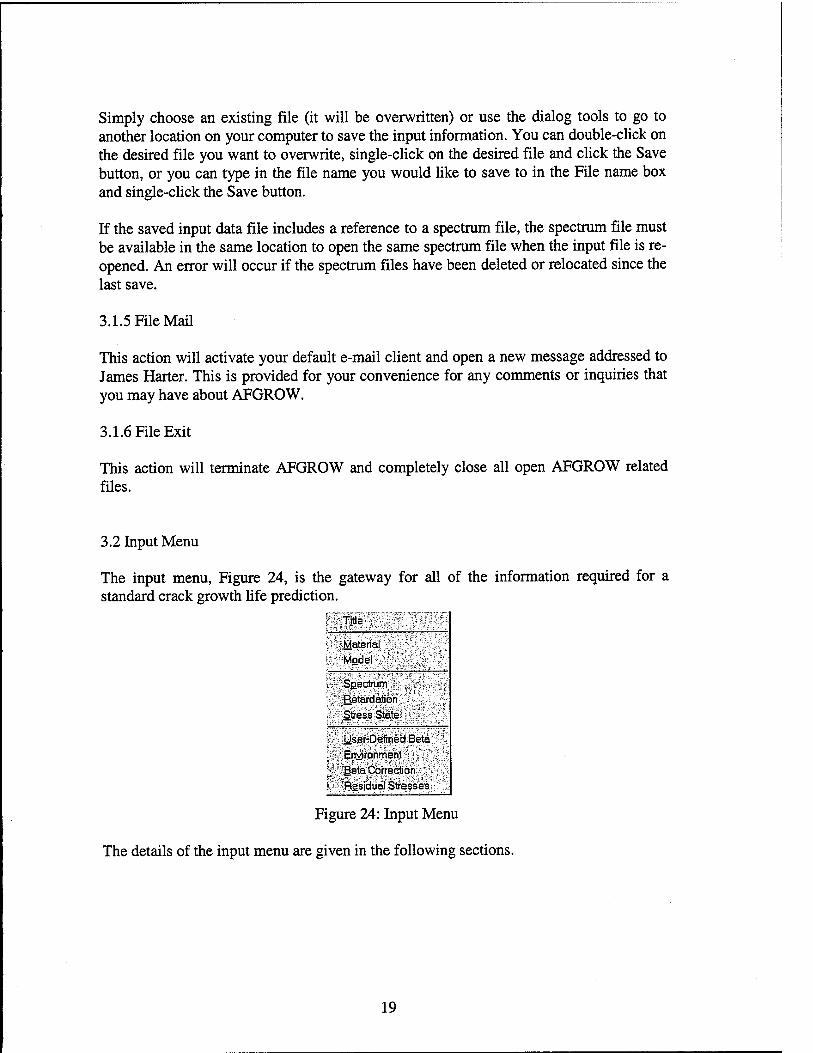
3.2 Input Menu
The input menu, Figure 24, is the gateway for all of the information required for a standard crack growth life prediction.
' rTitie" ""."" :
ffiateriaT JMddel /
Sßectaim
Retardation
Stress State
User-Defined Beta
Environment
Beta Correction
Residual Stresses
Figure 24: Input Menu
The details of the input menu are given in the following sections.
19
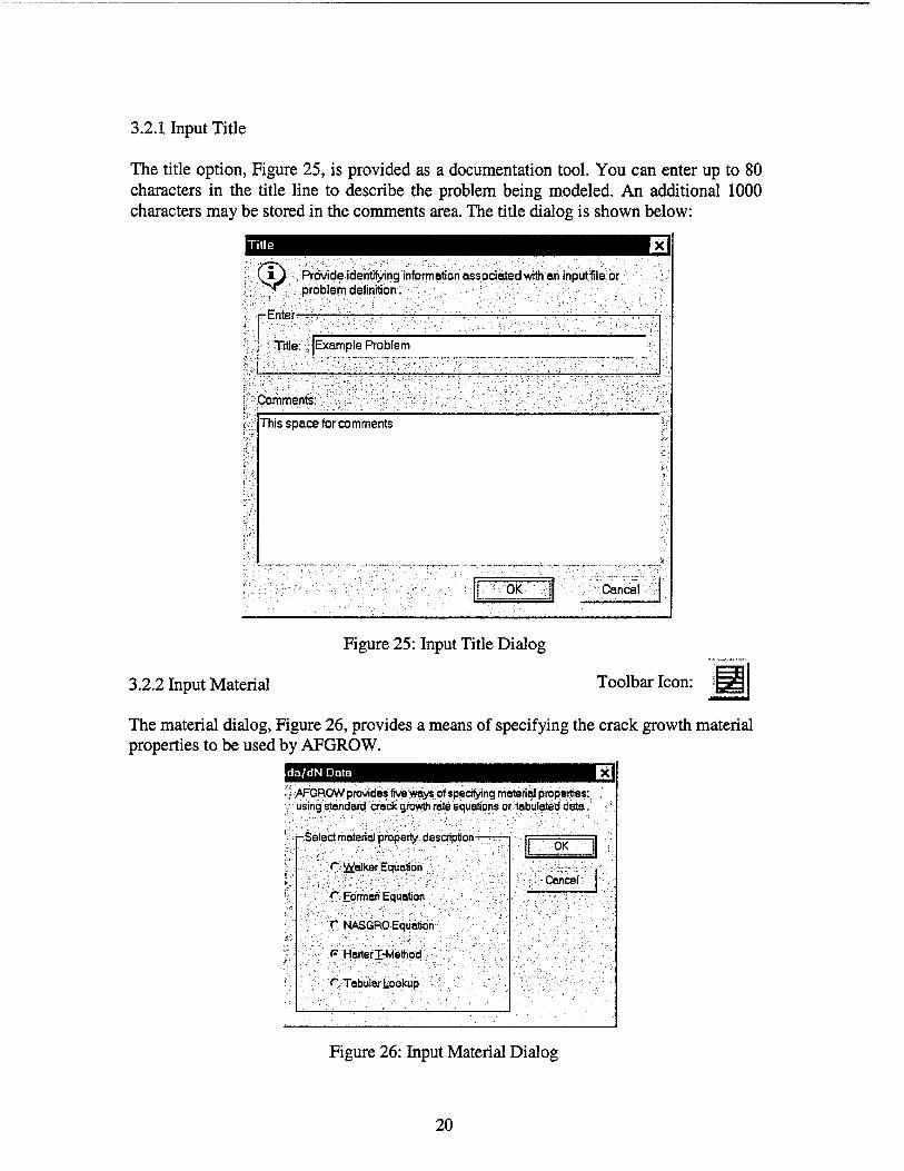
3.2.1 Input Title
The title option, Figure 25, is provided as a documentation tool. You can enter up to 80 characters in the title line to describe the problem being modeled. An additional 1000 characters may be stored in the comments area. The title dialog is shown below:
OO ■'v-FtbvideJderi^ngjnfbirnotionassodated-with'BnJnputfile.or ;*^ problem definition.
■Enter "'.■ ... ■■.,,, ■ :,' .. —■:-..: . —. ,.. ......... , ..
sTrtle: ijExample Problem
: Comments:
This space for comments
OK Cancel
Figure 25: Input Title Dialog
3.2.2 Input Material Toolbar Icon:
The material dialog, Figure 26, provides a means of specifying the crack growth material properties to be used by AFGROW.
da/dN Data
AFGROW provides five ways of speaking material properties: using standardcrack" growth rate equations or tabulated data.
-r.Select material property description ———
CW.alker Equation. ~
:P'.; CE°i™an Equation ■. ~';£.
f NASGRO Equation
P Harterl-Method
C. Tabular Lookup
OK
• Cancel >
Figure 26: Input Material Dialog
20

The following sections contain detailed descriptions of each of the methods used to determine crack growth material properties.
3.2.2.1 Walker Equation Walker Equation Data
^'YsiATheWalkerequatonextendBdlheeaiV Pans- equationbydlovflngiheshift:ihv N^ da/dN vs. Delta K as afundion of stress ratio (R). The equation may be used in
sevens! segments to attemptto model the sigmoidalshape of the data."
p.Ulse up to 5 sets of values of 'C.
! ' i Number of Sets- | 2
\ Set C -
n'. and 'm'
n m
- | 1 |2 6e-009 > |3 2 JO 5 _* > , I 1 2 " lle-008 Iff |3 ?;:JH 0-51
| 3 Jle-008 _
[T _ jle-008
|3 |0 5
|3 jo 5 .' | 5 ,'Jle-D08 -- |3 |0 5
• ;
"Material name: lUser defined data
f Coefficient of Thermal Expansion:-:]1.25e-005
Yield Strength. YLD: "56
fiPläne Stressfj*ÄrCT^ghr£s&KC: '(100
;;Plane"St>ÄnFra^iSTöügrmesbMC:fl35
.0eitaK*reshoid.value:@R-O : 2
Young's Modulus: J105Q0 %
Poisson's Rafio. Jo.33 j
Lower limit on R shift (p..-1). j-0 3
Upper limit on R shift (<1): P J
KOK'' .Cancel :.;Soye'; Read Apply!
Figure 27: Walker Equation Dialog
The Walker equation [12] was essentially an enhancement of the Paris Equation that included a means to account for the effect of Stress Ratio (Minimum Stress/Maximum Stress) on crack growth rate (see Figure 28).
s ■a s s. o
R: »-0 ,R = 0
n
/ / j / log(AK)
1
Figure 28: Walker Equation
21
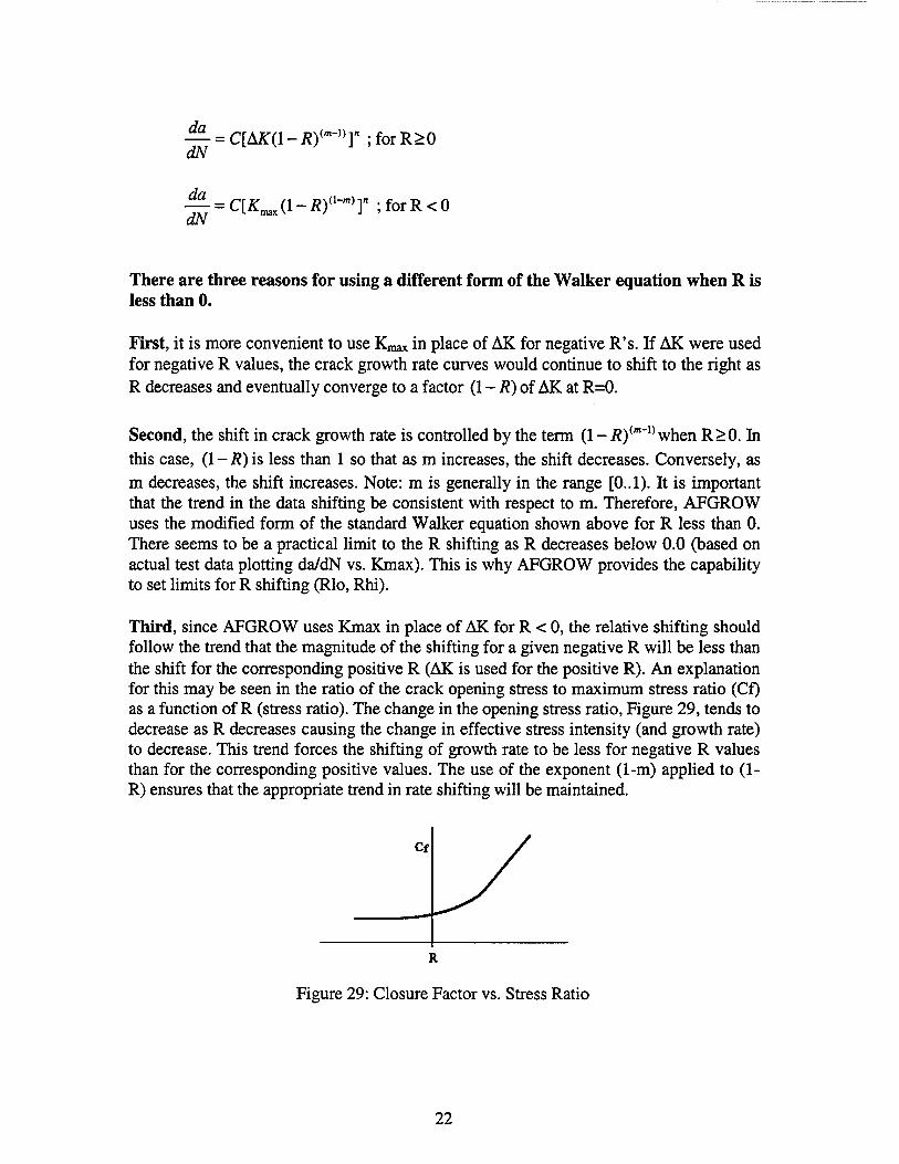
— = C[AK(1-Rym-1)T ;forR>0 dN
^ = C[Kmx(l-Rf-m)Y ;forR<0 dN
There are three reasons for using a different form of the Walker equation when R is less than 0.
First, it is more convenient to use K^ in place of AK for negative R's. If AK were used for negative R values, the crack growth rate curves would continue to shift to the right as R decreases and eventually converge to a factor (1 - R) of AK at R=0.
Second, the shift in crack growth rate is controlled by the term (1 - J"?)(m_1) when R>0. In this case, (1 - R) is less than 1 so that as m increases, the shift decreases. Conversely, as m decreases, the shift increases. Note: m is generally in the range [0..1). It is important that the trend in the data shifting be consistent with respect to m. Therefore, AFGROW uses the modified form of the standard Walker equation shown above for R less than 0. There seems to be a practical limit to the R shifting as R decreases below 0.0 (based on actual test data plotting da/dN vs. Kmax). This is why AFGROW provides the capability to set limits for R shifting (Rio, Rhi).
Third, since AFGROW uses Kmax in place of AK for R < 0, the relative shifting should follow the trend that the magnitude of the shifting for a given negative R will be less than the shift for the corresponding positive R (AK is used for the positive R). An explanation for this may be seen in the ratio of the crack opening stress to maximum stress ratio (Cf) as a function of R (stress ratio). The change in the opening stress ratio, Figure 29, tends to decrease as R decreases causing the change in effective stress intensity (and growth rate) to decrease. This trend forces the shifting of growth rate to be less for negative R values than for the corresponding positive values. The use of the exponent (1-m) applied to (1- R) ensures that the appropriate trend in rate shifting will be maintained.
R
Figure 29: Closure Factor vs. Stress Ratio
22
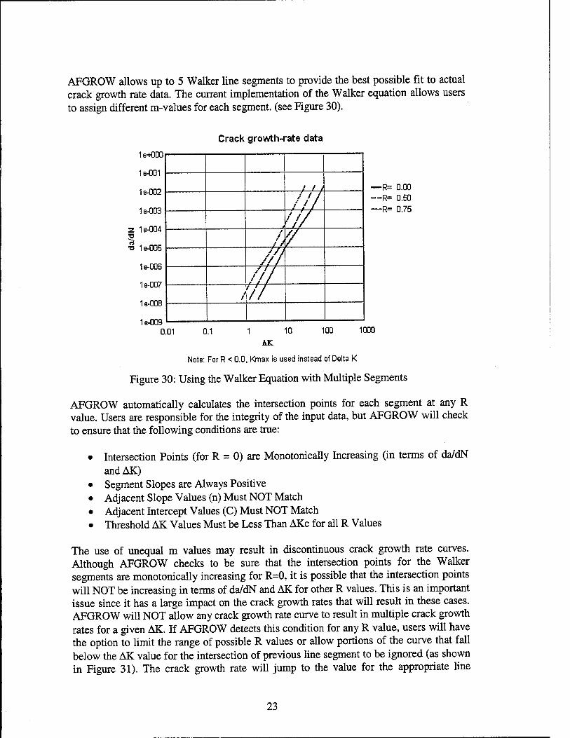
AFGROW allows up to 5 Walker line segments to provide the best possible fit to actual crack growth rate data. The current implementation of the Walker equation allows users to assign different m-values for each segment, (see Figure 30).
Crack growth-rate data
1e+O00
1 e-001
16-002
1e-003
1e-004
■3 1e-005
1e-006
1e-007
1e-008
1e-009
/ * i <l l /
1
'(/ 1 1 //
///
/ / '//
—R= 0.00 —R= 0.50 —R= 0.75
0.01 0.1 10 100 1000
AK
Note: ForR <0.0, Kmax is used instead of Delta K
Figure 30: Using the Walker Equation with Multiple Segments
AFGROW automatically calculates the intersection points for each segment at any R value. Users are responsible for the integrity of the input data, but AFGROW will check to ensure that the following conditions are true:
• Intersection Points (for R = 0) are Monotonically Increasing (in terms of da/dN andAK)
• Segment Slopes are Always Positive • Adj acent Slope Values (n) Must NOT Match • Adj acent Intercept Values (C) Must NOT Match • Threshold AK Values Must be Less Than AKc for all R Values
The use of unequal m values may result in discontinuous crack growth rate curves. Although AFGROW checks to be sure that the intersection points for the Walker segments are monotonically increasing for R=0, it is possible that the intersection points will NOT be increasing in terms of da/dN and AK for other R values. This is an important issue since it has a large impact on the crack growth rates that will result in these cases. AFGROW will NOT allow any crack growth rate curve to result in multiple crack growth rates for a given AK. If AFGROW detects this condition for any R value, users will have the option to limit the range of possible R values or allow portions of the curve that fall below the AK value for the intersection of previous line segment to be ignored (as shown in Figure 31). The crack growth rate will jump to the value for the appropriate line
23
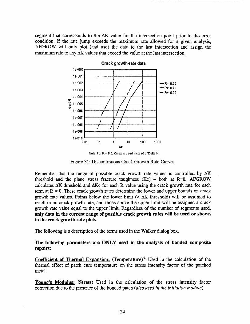
segment that corresponds to the AK value for the intersection point prior to the error condition. If the rate jump exceeds the maximum rate allowed for a given analysis, AFGROW will only plot (and use) the data to the last intersection and assign the maximum rate to any AK values that exceed the value at the last intersection.
Crack growth-rate data 1e+000
1e-001
1e-002
1e-003
1 e-004 z H 1e-005 ■o
1e-006
1e-007
1e-008
1e-009
1e-010
/ / / /
1 r / /
1 ' / > /
1 /
/ 1 / 1 1
/ 1 /
/ / / /
i * /
—R= 0.00 —R= 0.70 —R= 0.90
0.01 0.1 10 100 1000
AT
Note: For R < 0.0, Kmax is used instead of Delta K
Figure 31: Discontinuous Crack Growth Rate Curves
Remember that the range of possible crack growth rate values is controlled by AK threshold and the plane stress fracture toughness (Kc) - both at R=0. AFGROW calculates AK threshold and AKc for each R value using the crack growth rate for each term at R = 0. These crack growth rates determine the lower and upper bounds on crack growth rate values. Points below the lower limit (< AK threshold) will be assumed to result in no crack growth rate, and those above the upper limit will be assigned a crack growth rate value equal to the upper limit. Regardless of the number of segments used, only data in the current range of possible crack growth rates will be used or shown in the crack growth rate plots.
The following is a description of the terms used in the Walker dialog box.
The following parameters are ONLY used in the analysis of bonded composite repairs:
Coefficient of Thermal Expansion: (Temperature)"1 Used in the calculation of the thermal effect of patch cure temperature on the stress intensity factor of the patched metal.
Young's Modulus: (Stress) Used in the calculation of the stress intensity factor correction due to the presence of the bonded patch (also used in the initiation module).
24

Poisson's Ratio: (Non-Dimensional) Used in the calculation of the stress intensity factor correction due to the presence of the bonded patch.
The following parameters are used in the standard crack growth analysis:
C: (Stress('n), Length04"2*) Value of da/dN when R=0 and Delta K=l (da/dN intercept).
n: (Non-Dimensional) Paris Exponent (da/dN slope).
Walker Exponent, m: (Non-Dimensional) Normal Range (0-1) Controls shift in crack growth rate data, curve shift decreases as m increases.
Plane Stress Fracture Toughness (KC): (Stress, Length0-5) Value of Fracture Toughness to be used under pure plane stress conditions.
Plane Strain Fracture Toughness (KIC): (Stress, Length0,5) Value of Fracture Toughness to be used under pure plane strain conditions.
Delta K Threshold Value @ R=0. THOLD: (Stress, Length0,5) Threshold stress intensity value at R=0 - no crack growth will be calculated when Delta K is below threshold for a given R value.
Yield Strength. YLD: (Stress) Yield stress (0.2% strain) for the metal being analyzed.
Lower limit on R shift, Rio: (Non-Dimensional) R value below which no further R shifting is calculated.
Upper limit on R shift. Rhi: (Non-Dimensional) R value above which no further R shifting is calculated.
Buttons:
APPLY: Apply the current parameters.
READ: Read a file containing Walker parameters.
SAVE: Save the current parameters to a file.
CANCEL: Cancel the dialog box.
OK: Accept the current parameters and close the dialog box.
25
3.2.2.2 Forman Equation Material- Forman Equation
Malarial Properties Forman Constants I
pEnter—rr——, ;—;—:— ——,■: ■, ■■ ..■■
DeraKthresholdvalueSR-O.THOLD: |2
. Upper limit on R shift. RHI (Max 1.0): [Ö75 , RCUT: |C -
. Lower limit on R shift RLÖ(0_. -4.0): |-1
rSelect-
fiEJIIB- ,if K <-R<- 1
^Formen Curve to
Number of Sets:
.■:'-:S«it'''ff,:C-:;-
RLO<- H<- R CUT——-,
Kcut
>KC .y;,.;; n 4,
]r |2.6e-009 J3-2 4 .IN'. k ■ :,,K ^■y- , \i: . I1
P Formen Curve for RCUT< R <- RHI
i ;■/:': Numberof Sets: 10 ;'-S«'T:'.^C'V.'; V/-n '
-Iff IT IT
i
OK Cancel läpp*/ Save. :Read
Figure 32: Forman Equation Dialog
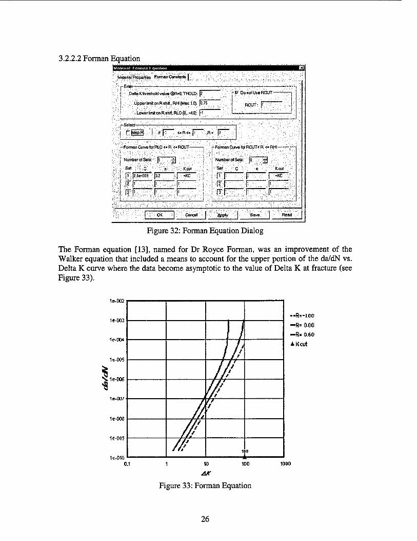
The Forman equation [13], named for Dr Royce Forman, was an improvement of the Walker equation that included a means to account for the upper portion of the da/dN vs. Delta K curve where the data become asymptotic to the value of Delta K at fracture (see Figure 33).
1B-DCC
1e-CC3
1e-CO*
1s.005
Sle-0C6
1e-CU/
le-C08
1C-O05
1e-O10
) /i I ft iff I ft If* / f* f ft
f ft if* fff 'ft
///
ft /
Iff ff* f f* ff* f ft 1
1 i 10
V «
--R—I.00
-R= 0.00
—R= 0.60
4 Kcut
0.1 10
AK
100 1000
Figure 33: Forman Equation
26

The form of the Forman equation used in AFGROW is shown here.
da
~dN
CAK"
{{1-R)KC-AK)
A weakness of the Forman equation lies in a lack of flexibility in modeling data shifting as a function of stress ratio (R). There is no parameter to adjust the R shift directly. The amount of shifting is controlled by the plane stress fracture toughness of a given material.
The material properties, used with the Forman equation, are accessible in a separate tab of the Forman dialog box as shown in Figure 34 (simply click on the material properties tab):
Material- Forman Equation
:.1ylatBn#RropBtties;.|Formm Constants]'i
® Delta K behavior :'/TheEquation results iftlihear behavior in log^ogspeceinthetowand mind-range; and;:; Sailowstheupperendofthedatatocurveupvrardmodelingftenear-lailurebeh'aviorof ".
melals
center,,. ;:,,Y. '.-..;.-;;;
Matenal Name
y^iiW&'&ff-'is i-jUser defined data
Coefficient of Thermal Expansion:
Young's Modulus:
W^^:,SfSS;S*;SSftÄ'8'R&
Yield- Strength. YLD~: '
.Plane Strain Fracture Toughne"ss.KIC:::.
i: Plane Stress Fracture Toughness.:KC:-
1.2SB-0G5 : ■■-.";■
10500 jV-;',
0.33 -:; •;
66
|35 £:>y.
ioo ;;'-;..
OK- Cancel j^Sply ;i I ': fvgave ] .Read
Figure 34: Forman Equation Material Property Dialog
AFGROW allows up to 3 Forman segments (or sets - see Figure 32) to provide the best possible fit to actual crack growth rate data. Users are permitted to define up to 2 fits (3 segments each) as a function of stress ratio (R). If a second fit is desired for R greater than a given value (Rcut), simply uncheck the [Do not Use RCUT] box and enter the desired Rcut value in the appropriate field. AFGROW also allows users to map the Forman fit for a given R to a range of R-values. This option may be useful if users would like to limit the R shift to a certain value. It should be noted that although the Forman equation uses the Paris equation in its numerator, it IS NOT equivalent to the Paris equation because of the terms in the denominator. It is important to note here that when using the Forman equation, AFGROW allows the use of Delta K to include negative K when R < 0.0. This is the ONLY exception to the normal standard in AFGROW. This exception results in a shift in crack growth rate data to the right of the R= 0.0 data when R < 0.0.
27

The current Forman dialog provides a GREAT deal of flexibility in handling crack growth rate data with a closed-form equation.
The following parameters are ONLY used in the analysis of bonded composite repairs:
Coefficient of Thermal Expansion: (Temperature)-1 Used in the calculation of the thermal effect of patch cure temperature on the stress intensity factor of the patched metal.
Young's Modulus: (Stress) Used in the calculation of the stress intensity factor correction due to the presence of the bonded patch {also used in the initiation module).
Poisson's Ratio: (Non-Dimensional) Used in the calculation of the stress intensity factor correction due to the presence of the bonded patch.
The following parameters are used in the standard crack growth analysis:
C: (Stress(1"n), Length((3'n)y2)) Value of da/dN * (Kc-1) when R=0 and Delta K=l.
n: (Non-Dimensional) Paris Exponent (in this case, limit in da/dN slope as AK approaches 0.0).
Rcut: (Non-Dimensional) Value of Stress Ratio (R) defining the highest R allowed for the first Forman curve fit (leftmost curve fit in Forman Constants dialog box).
Kcut: (Stress, Length0-5) Value of Delta K (at R=0) defining the highest Delta K allowed for the given segment (upper segment boundary) - Note, the Kcut for the last defined segment is assumed to be equal to the plane stress fracture toughness of the metal being analyzed.
Plane Strain Fracture Toughness (KIC): (Stress, Length05) Value of Fracture Toughness to be used under pure plane strain conditions.
Plane Stress Fracture Toughness (KC): (Stress, Length0-5) Value of Fracture Toughness to be used under pure plane stress conditions.
Yield Strength, YLD: (Stress) Yield stress (0.2% strain) for the metal being analyzed.
The following parameters may be used in the retardation models in AFGROW:
Delta K Threshold Value @ R=0. THOLD: (Stress, Length03) Threshold stress intensity value at R=0 - this parameter is required by the Willenborg retardation model. It is NOT currently used in crack growth rate calculations. At this time, there is no lower bound on da/dN in the Forman equation in AFGROW. The only limit occurs when the
28

total crack growth after one spectrum pass is < 1.0E-13 (in whatever length units are being used).
Lower limit on R shift, Rio; (Non-Dimensional) R value below which no further R shifting is calculated.
Upper limit on R shift, Rhi: (Non-Dimensional) R-value above which no further R shifting is calculated.
Buttons:
OK: Accept the current parameters and close the dialog box.
CANCEL: Cancel the dialog box.
APPLY: Apply the current parameters.
SAVE: Save the current parameters to a file.
READ: Read a file containing Forman parameters.
29
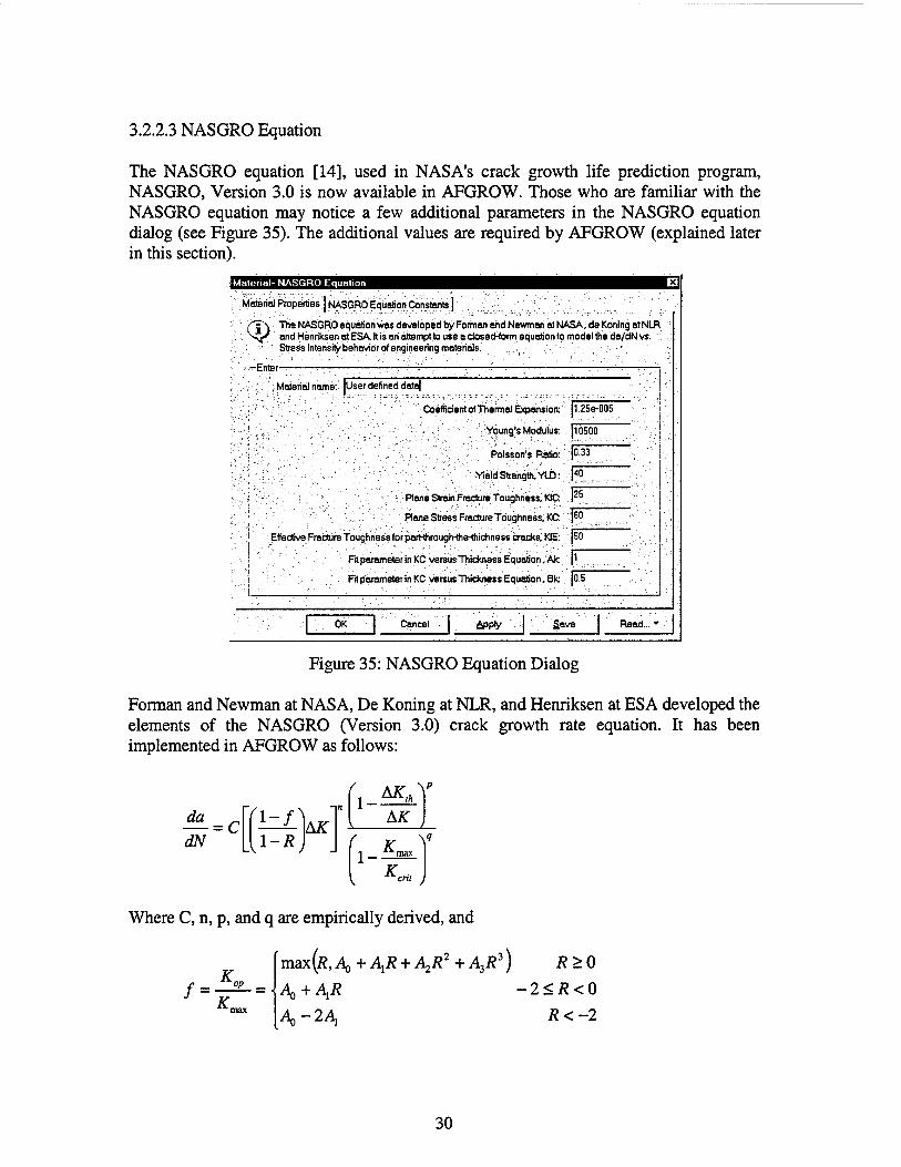
3.2.2.3 NASGRO Equation
The NASGRO equation [14], used in NASA's crack growth life prediction program, NASGRO, Version 3.0 is now available in AFGROW. Those who are familiar with the NASGRO equation may notice a few additional parameters in the NASGRO equation dialog (see Figure 35). The additional values are required by AFGROW (explained later in this section).
Material- NASGRO Equation
Material Properties | NASGRO Equation Constants |
®. The NASGRO equation was developed by Formen and Newman at NASA, de Koning at NLR and Henriksen at ESA. It is an attempt to use a dosed-form equation to model the da/dN vs. , Stess Intensity behavior of engineering matenals.
^Enter^—-—-. r-r ; —. : ■—■ : : -—— : ■ — j
:':' ■;. Material name: lUser defined data|
Coeffident of Thermal Expansion:
:1 xv'::'':'\ ' ■;".; '.r;.Vpung"* Modulus:
■■■'..';;.■/.'-. ., Poisson's Ratio:
■\r.:-.;./.:^;':.:•.'.' Yield Strength, YLD:
■ -. Plane Strain Fracture Toughness. KIC
Plane Stress Fracture Toughness. KG
Effective Fracture Toughness for parHhrough-the-thichness cracks. KlE:
Fit parameter in KC versus Thickness Equation. Ale
Fit parameter in KC versus Thickness Equation; Bk
-.-.-■
1.25e-005 y ■■-■:j
|10500
JO.33 \ \
\A0
P„ |60
|50 -; ,.,"-.|
h v I 1°5 ,;.,:.-i
OK Cancel Apply Save Read... »;■
Figure 35: NASGRO Equation Dialog
Forman and Newman at NASA, De Koning at NLR, and Henriksen at ESA developed the elements of the NASGRO (Version 3.0) crack growth rate equation. It has been implemented in AFGROW as follows:
da
IN = c
1-R AK
( AK Y
( K I _ max V
K,
Where C, n, p, and q are empirically derived, and
'max(/?,A0+A1i? + A!/?2+A3Ä3) R>0
■A0 + A1R -2<R<0
A3-2A, R<-2
f-K°p -
30

The coefficients are:
4o = (0.825-0.34a + 0.05a2] cod ^-S^la, JJ
A = (0.415-0.07^)5^/<70
^=l-4,-A1-A3
A3 = 2Ao + A1 -1
Here, a is the plane stress/strain constraint factor, and Smax/Go is the ratio of the maximum applied stress to the flow stress. These values are provided by the NASGRO material database for each material.
AK,U = AK, a
\ a + a o
M ( I 1-/
\(l+C,AK)
(I-A,XI-ä)J
Where:
• AKo - threshold stress intensity range at R = 0 • a - crack length (a or c in AFGROW) • a0 - intrinsic crack length (0.0015 inches or 0.0000381 meters) • Cth - threshold coefficient
The values for AKo and Cth are provided by the NASGRO material database for each material.
The NASGRO equation accounts for thickness effects by the use of the critical stress intensity factor, Kcrit.
KIC
Where:
• Kic - plane strain fracture toughness (Mode I) • Ak - Fit Parameter • Bk - Fit Parameter • t - thickness • t0 - reference thickness (plane strain condition)
31
The plane strain condition is:
t0=2.5{KIC/(jJ
The values for Kic, Ak, and Bk are provided by the NASGRO material database for each material.
For part-through cracks, the NASGRO equation uses a variable, Kfc (in the database), in place of Kent- The value, Kie, is a material constant since the developers of the NASGRO equation felt that the Kent value of a part-through crack is not highly dependent on thickness. The value, Kent, is calculated internally and is ONLY used by AFGROW to determine da/dN. It is NOT used as a failure criterion. The variable, Kc, printed in the dialog box is NOT the Kent shown above (see note1 below).
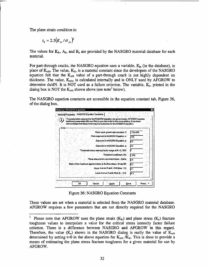
The NASGRO equation constants are accessible in the equation constant tab, Figure 36, of the dialog box.
Material- NASGRO Equation
Material Properties NASGRO Equation Constants I
"§ The parameters required forthe NASGRO equation are given below. AFGROW requires oddtonalparometBrs(RhiandRlo)toprovidelimitsforthecuiveshitting.lthasbeen demonstratedthettheselirrtemaybenecessaiytortheNASGROequBlion. :
- Enter —^—:———■——— r-—■ ■—.
Peris crack growth rate constant C
Paris exponent in NASGRO Equation, n.
Exponent in NASGRO Equation, p:
Exponent in NASGRO Equation, q:
Threshold stress intensiy factor range at R"0.DKD:
Threshold coefficient Cth:
Plane stress/strain constraint factor. Alpha:
Ratio of the maximum applied stress to the flow stress. Smax/SO:
Upper limrt on R shift. RHI (Max 1.0):
Lower limit on R shift RLO (0...-2.0):
|l.32e-009
|2.95
■V*
P* I7
|1.506
;'-M...... -;■• ■■ |0.3
|0.7
.i°-3......
OK - Cancel "< Apply : 'Save Read...''
Figure 36: NASGRO Equation Constants
These values are set when a material is selected from the NASGRO material database. AFGROW requires a few parameters that are not directly required for the NASGRO
1 Please note that AFGROW uses the plane strain (Kj.c) and plane stress (Kc) fracture toughness values to interpolate a value for the critical stress intensity factor failure criterion. There is a difference between NASGRO and AFGROW in this regard. Therefore, the value (Kc) shown in the NASGRO dialog is really the value of Kent determined by setting t=0 in the above equation for Kent /Kfc. This is done to provide a means of estimating the plane stress fracture toughness for a given material for use by AFGROW.
32
equation. AFGROW uses the variables Rio and Rhi to set stress ratio limits. It was discovered that the parameters for many of the materials in the NASGRO database would cause the crack growth rate curves to behave erratically above or below certain stress ratios. The crack growth rate curves can become vertical (Ka = Kent)- To avoid this, AFGROW will check for this problem and automatically set Rhi and Rio when a material is selected. If parameters are edited manually, care should be taken to verify that this problem will not occur (use the da/dN vs. Delta K plot view in the main frame - see section 2.1.3).
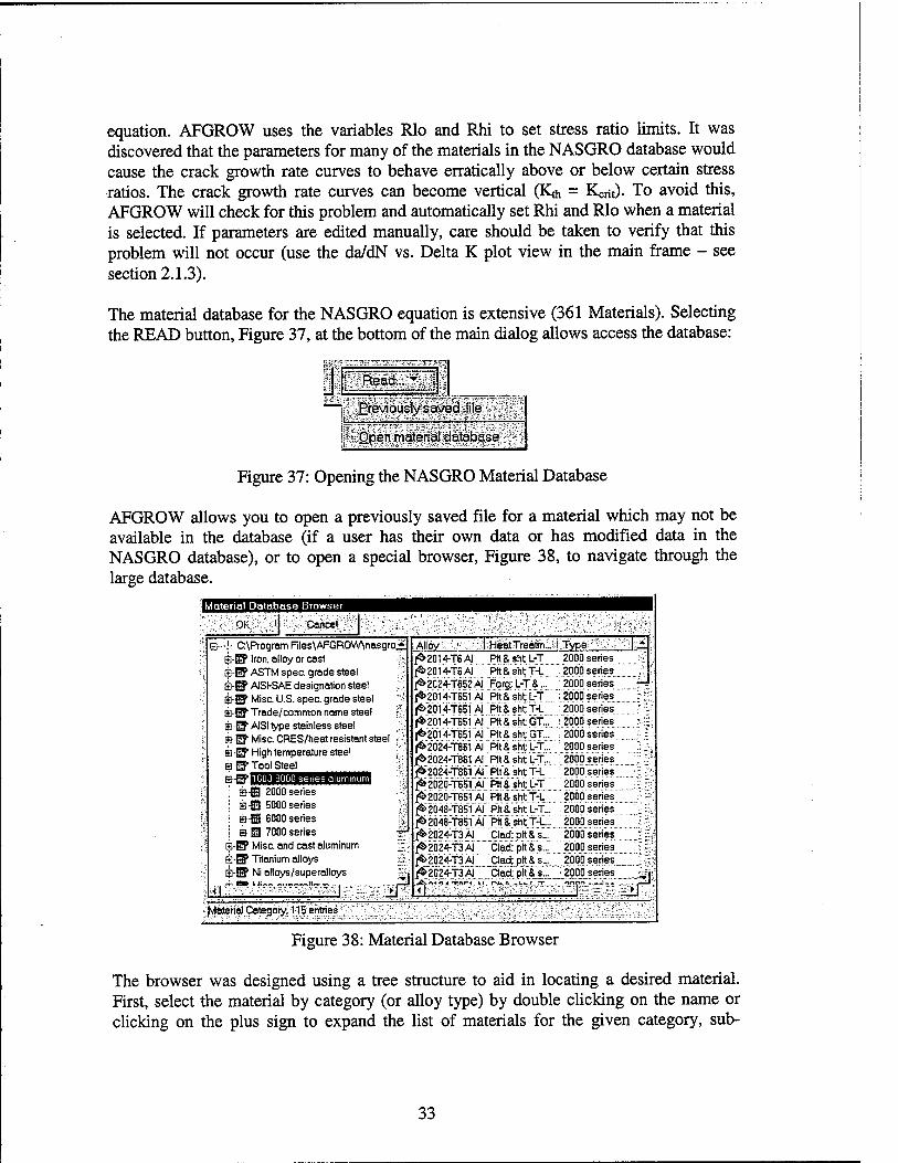
The material database for the NASGRO equation is extensive (361 Materials). Selecting the READ button, Figure 37, at the bottom of the main dialog allows access the database:
JE ffiö^ÄK 4— Previously saved -file
Open material database
Figure 37: Opening the NASGRO Material Database
AFGROW allows you to open a previously saved file for a material which may not be available in the database (if a user has their own data or has modified data in the NASGRO database), or to open a special browser, Figure 38, to navigate through the large database.
Material Database Browser
yafv: Cancel
E-l- C:\Program Files\AFGROW\nasgroii $1P Iron, alloy or cast B-B1 ASTM spec, grade steel BW AISI-SAE designation steel B-W Misc. U.S. spec, grade steel £?. mS Trade/common name steel ;S B W AISI type stainless steel ffl-llP Misc. CRES/heat resistant steel A ffi-ip High temperature steel B W Tool Steel
s-fHSEBOIBi I ; g}-fl 20Ö0 series ' I B-l 5000 series V i H~B 6000 series if? I &-H 7000 series £■ B-W Misc. and cast aluminum E i-B Titanium alloys '£ EJ3-B' Ni alloys/superalloys
ill ■J>.
Alloy t;<?'i^:;]iHeatirreätrri:- fS>2014-T6AI Plt&shtL-T 1*2014-T6 Al Pit 8. shf f-L J*2Ö24-T852ÄI Forg; L-f &... j<6> 2014-tBSI ÄI Pit & sht L-f jfS'201 4-f 651 Al' Pit & sht f-L j^2Öi4-t65iÄi Pit&shtGf .. 1*2014-T651 ÄI Pit 8. sht GT... j&20'24-f861 Ai Pit 8. sht L-f... ^2024-7861 Ai Pit8^shtL-f... ^2024-f86i Ai Pit 8, sht f-L f*2020-T651 Al Pit8, sht L-T /&202Ö-T651 AiPit &"sht' f-L ^2048-f85iÄi Pit 8. sht L-f... 1* 2048-f851 Ai Pit. & sht f-L... j&202+f3ÄI äad;plt&s... J&2024-T 3Ä1 Clad; pit & s... f*2024-T3AI _Clad:j)lt8,s...
.>6S.^'lÖ.<.*T'rit"H * I. TNI», ft...-i.». ..I.....-T.....
|;Type : 2000 series 2000 series 2000 series
; 2000 series : JOpOseries ; 2000 series
2000 series ^2000 series [2tjb0series
2000 series 2Ö0Öseries
' 2000 series : 2000i series [2Ö0Öseries
2000 series 2000 series 2000 series
:TÖÖÖ series IU series _ ™i!
Material Category. 115^ entries'
Figure 38: Material Database Browser
The browser was designed using a tree structure to aid in locating a desired material. First, select the material by category (or alloy type) by double clicking on the name or clicking on the plus sign to expand the list of materials for the given category, sub-
33
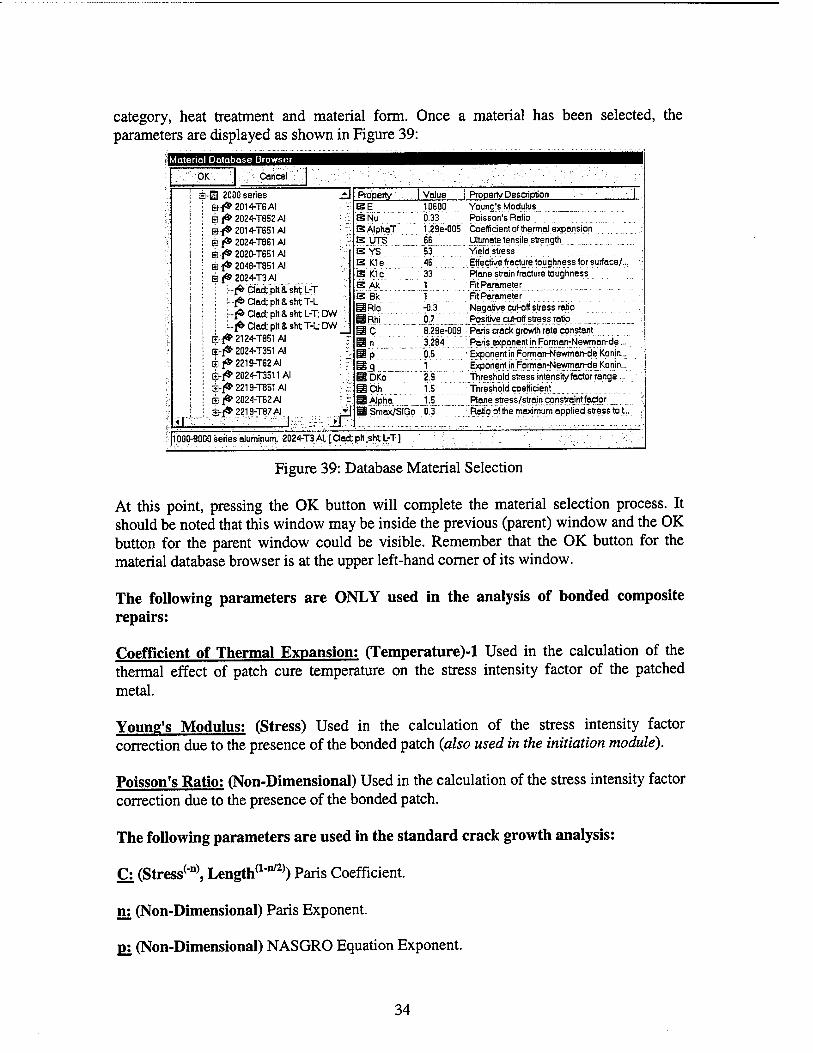
category, heat treatment and material form. Once a material has been selected, the parameters are displayed as shown in Figure 39:
Material Database Browser
Cancel OK'
; it-
I $• I E
: & ! m- '■ B
2000 series f»2014-T6AI /»2024-T852AI (»2014-T651AI [* 2024-T861 Al J* 2020-T651 Al •1* 2048-T851 Al fS>2024-T3AI
i f* ä'ad; ptt& shtVT i f8> Clad; plt& sht T-l !-■{* Clad: pit &shtL-T;DW :-lfeaad:pltashtT-UDW
f«>2124-T851AI ■■(* 2024-T351 Al 1»2219-T62AI |* 2024-T3511 Al J*2219-T851AI f«>2024-T62AI f* 2219-T87 Al
Property [ Value | Property Description BE 10600 ENu 0.33 SAIphaT 1.29e-005 IS UTS 66 SYS 53 E Kle 46 E Kle 33 E Ak 1 B Bk 1 gRIo -0.3 ÜRhi 07 ic 8.29e-009 Ü n 3.284 §p 0.5
SDKo 1
ÜCth 1.5 S Alpha ü "Smax/SIGo
1.5 ' 0.3
Young's Modulus Poisson's Ratio Coefficient of thermal expansion Ultimate tensile strength Yield stress Effective fracture toughness for surface/... Plane strain fracture toughness Fit Parameter _ FrtParameter Negative cut-off stress ratio
Paris crack growth rate constant Paris exponent in FormarrNevyman-de...
* Exponent in Forman-Newman-de Konin... ExponentjnFonria^ewman-de Konin... threshold stress intensiv factor range... Threshold coefficient Plane stress/strajn cpnsfrajnt factor Ratio of the maximum applied stress to t..
100MOO0 series aluminum. 2021-T3AI.faad.plt shtL-T]
Figure 39: Database Material Selection
At this point, pressing the OK button will complete the material selection process. It should be noted that this window may be inside the previous (parent) window and the OK button for the parent window could be visible. Remember that the OK button for the material database browser is at the upper left-hand corner of its window.
The following parameters are ONLY used in the analysis of bonded composite repairs:
Coefficient of Thermal Expansion: (Temperature)-1 Used in the calculation of the thermal effect of patch cure temperature on the stress intensity factor of the patched metal.
Young's Modulus: (Stress) Used in the calculation of the stress intensity factor correction due to the presence of the bonded patch (also used in the initiation module).
Poisson's Ratio: (Non-Dimensional) Used in the calculation of the stress intensity factor correction due to the presence of the bonded patch.
The following parameters are used in the standard crack growth analysis:
C: (Stress('n), Length*1^) Paris Coefficient.
n: (Non-Dimensional) Paris Exponent.
P2 (Non-Dimensional) NASGRO Equation Exponent.
34
Q: (Non-Dimensional) NASGRO Equation Exponent.
C^: (Non-Dimensional) Threshold Coefficient.
Alpha: (Non-Dimensional) Plane stress/strain constraint factor.
Smax/gn: (Non-Dimensional) Maximum applied stress to flow stress ratio.
Yield Strength. YLD: (Stress) Yield stress (0.2% strain) for the metal being analyzed.
Plane Strain Fracture Toughness (KIC): (Stress, Length05) Value of Fracture Toughness to be used under pure plane strain conditions.
Plane Stress Fracture Toughness (KC): (Stress, Length05) Value of Fracture Toughness to be used under pure plane stress conditions.
Kisl (Stress, Length0,5) Effective fracture toughness for part through-the-thickness cracks - ONLY used in place of Kcrit in the NASGRO equation for crack growth rate calculations for part through-the-thickness cracks (not a failure criterion).
Ak: (Non-Dimensional) Fit parameter in Kcrit/KIc vs. thickness equation.
Bk: (Non-Dimensional) Fit parameter in Kcrit/KIc vs. thickness equation.
The following parameters may be used in the retardation models in AFGROW:
AKO: (Stress, Length0-5) Threshold stress intensity factor range at R=0.
Rio; (Non-Dimensional) Lower limit on R shift.
Rhi; (Non-Dimensional) Upper limit on R shift.
Buttons:
OK: Accept the current parameters and close the dialog box.
CANCEL: Cancel the dialog box.
APPLY: Apply the current parameters.
SAVE: Save the current parameters to a file.
READ: Read the NASGRO material database OR a file containing NASGRO equation parameters.
35
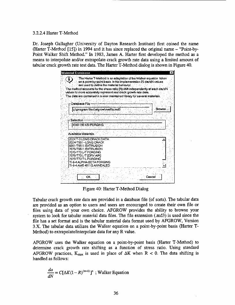
3.2.2.4 Harter T-Method
Dr. Joseph Gallagher (University of Dayton Research Institute) first coined the name (Harter T-Method [15]) in 1994 and it has since replaced the original name - "Point-by- Point Walker Shift Method." In 1983, James A. Harter first developed the method as a means to interpolate and/or extrapolate crack growth rate data using a limited amount of tabular crack growth rate test data. The Harter T-Method dialog is shown in Figure 40.
Material Database
(j[\ TheHarter T-Method is an adaptation of the Walker equation taken ^T- on a point-by-point basis. Inthis implementation 25 da/dN values
are used to define the material behavior. The method accounts-forthe stress ratio (R) shift independently at each da/dN values to'more accurately represent real crack growth rate data The dataare contained in ausermaintainedlibraryforseveral materials.
-Database File-
|c:\program files\afgröw\rhatfile.md3 . Browse.
r^'Selectiori- M340-180KSI FORGING
Available Materials:
2024 T-3 LONG CRACK DATA .A.
2024-T851 - LONG CRACK 6061-T6511 EXTRUSION 7075-T6511 EXTRUSION 7075-T73 L-T FORGING 7075-T73L-T[DRYAIR] 7075-T73T-L FORGING __ Ti-6-4 ALPHA-BETA FORGING Ti-6-4 AMS 4911G ANNEALED ^
OK Cancel
Figure 40: Harter T-Method Dialog
Tabular crack growth rate data are provided in a database file (of sorts). The tabular data are provided as an option to users and users are encouraged to create their own file or files using data of your own choice. AFGROW provides the ability to browse your system to look for tabular material data files. The file extension (.md3) is used since the file has a set format and is the tabular material data format used by AFGROW, Version 3.X. The tabular data utilizes the Walker equation on a point-by-point basis (Harter T- Method) to extrapolate/interpolate data for any R value.
AFGROW uses the Walker equation on a point-by-point basis (Harter T-Method) to determine crack growth rate shifting as a function of stress ratio. Using standard AFGROW practices, Kmax is used in place of AK when R < 0. The data shifting is handled as follows:
— = C[AK(l - /?)(m-1>]" ; Walker Equation dN
36

At a given da/dN, the relationship reduces to:
AK = AKRJ1 ~ Rf~m) ; for R> 0.0
^max=A^Ä=o(l-^)(m"1);forR<0.0
Note that K^ is used in place of AK when R < 0. Although not algebraically correct, it is important that the proper trend in R shift be maintained. This trend is that as m increases, the R shift decreases. This method is simply a way to interpolate/extrapolate data in log- log scale by using the exponential form. This method has given very good results over the years.
It is usually very difficult to obtain crack growth rate data over a sufficient range of crack growth rate and R values to allow the use of simple interpolation methods to accurately model material behavior. A matrix large enough to allow that would consist of actual test data for at least 7 decades of crack growth rate, several R values (positive and negative), and cover the entire range of rate and R values required for the spectrum being analyzed. The Harter T-Method, Figure 41, allows the use of as much data as is available (of course, more data is better) and experience is very useful when data are limited.
Here's how it works:
Jog(da?dN)
fc>g(AK)
Figure 41: Harter T-Method Crack Growth Rate Shifting as a Function of R
Using the Walker equation (see above) at a single crack growth rate for two positive R values, the following relationship is seen:
AK^l-Rj^^AK^l-Rj"-1'
Solving for m yields:
m = l+ log10 AK,
/log 10 (l-*2)" ;forRiandR2>0
37

For the reasons stated above, the method to handle negative stress ratios simply involves using Kmax in place of AK and switching the exponent for the negative R as follows:
Solving for m yields:
m=l + log (K ^ ■"■maxi
10 AK, /log10((l -Rx)(\-R2)) ; Where Ri< 0.0 and R2>0.0
For two negative R values, the relationship becomes:
^maxl(1-Äl) m =KmaX2\}-~R2)
Solving for m yields:
ra = l- log (K, ^
10 maxl /log 10 l(l-Ä,)Jj
; Where Ri< 0.0 and R2< 0.0
It is important to know the significance of the value of m. The value, m, is non- dimensional and has no real physical significance. The value of m is merely a mathematical means of controlling the shift of the crack growth rate data as a function of stress ratio (R).
The n (slope) value in the Walker Equation gets cancelled when the equations for 2 R values are set equal at a given da/dN. All m does is provide a means of determining the R shift on a point by point basis. All that is required is to take AK (or Kmax if R<0) for two R values at the same crack growth rate, apply the appropriate equation, and an appropriate m may be calculated for the given crack growth rate. This method may be repeated at several rate values to describe the tabular data for any R value. AFGROW uses da/dN and Delta K (for R=0) and m at 25 crack growth rate values (da/dN) to recreate the da/dN, Delta K (or Kmax) curve for any R desired using the method described above. However, the recreated data are determined for the same rate values in the input table. AFGROW calculates the curve (really just the AKs or Kmax) for each rate until the K value exceeds the current K value of interest. Then it just does a logrithmic interpolation between the last two points in the curve (points on each side of the current stress intensity) to give the current rate. This can save a great deal of CPU time.
There are a few RULES that should be adhered to:
• Kmax is used in place of Delta K when R < 0.0 - All curves shift left of R=0.0 • Normally, the R shift for negative R values will stop for R < [-0.2 to -0.5] (Rio)
38
• It is NOT advisable to use data for R < Rio to determine m values • Normal range for m is [0-1] • Rio may be determined using m values determined for R values > -0.2 by finding
which negative R returns the curve for R < -0.5 • Shift for positive R is > negative R values for the same absolute R value • For adjacent points, m should not change abruptly
The format that is required for the material data file [filename.md3] is as follows (space delimited):
[Title] (up to 35 characters - should include units being used)
[da/dN] [Delta K @ R=0.0] [m] (25 lines of these data - EXACTLY 25 lines)
[Bio] [Bhi] [KIC] [Yield]
[Modulus] [Poisson's ratio] [Coefficient of Thermal Expansion]
The above is repeated for each material in the file. The LAST line requires the word, END to denote the end of material data. See additional notes2 on the use of this method in AFGROW
The following parameters are ONLY used in the analysis of bonded composite repairs:
Coefficient of Thermal Expansion: (Temperature)-l Used in the calculation of the thermal effect of patch cure temperature on the stress intensity factor of the patched metal.
Young's Modulus: (Stress) Used in the calculation of the stress intensity factor correction due to the presence of the bonded patch (also used in the initiation module).
Poisson's Ratio: (Non-Dimensional) Used in the calculation of the stress intensity factor correction due to the presence of the bonded patch.
2 When using the Harter T-Method in AFGROW, the threshold value of Delta K is taken to be the Delta K value (for R=0) corresponding to the lowest rate value of the table. AFGROW handles the shifting for the current R value internally. The maximum Delta K value for R=0.0 in the tabular data is assumed to be the plane tress fracture toughness (Kc) which is used to determine fracture under pure Plane Stress conditions. AFGROW expects 25 values of crack growth rate, Delta K (at R=0.0), and m. Please be sure to use 25 points, no more or less! For now, the units for this method MUST be English (Ksi, inches, degrees F). The conversion to metric units will be done by AFGROW internally if required.
39

The following parameters are used in the standard crack growth analysis:
Walker Exponent, m: (Non-Dimensional) Normal Range (0-1) Controls shift in crack growth rate data - curve shift decreases as m increases.
Plane Strain Fracture Toughness (KIC): (Stress, Length0'5) Value of Fracture Toughness to be used under pure plane strain conditions.
Delta K Threshold Value @ R=0, THOLD: (Stress, Length0"5) Threshold stress intensity value at R=0 - no crack growth will be calculated when Delta K is below threshold for a given R value.
Yield Strength, YLD: (Stress) Yield stress (0.2% strain) for the metal being analyzed.
Rio: (Non-Dimensional) R value below which no further R shifting is calculated.
Rhi: (Non-Dimensional) R value above which no further R shifting is calculated.
Buttons:
BROWSE: Browse system to find *.md3 files.
CANCEL: Cancel the dialog box.
OK: Except the current choice and close the dialog box.
40
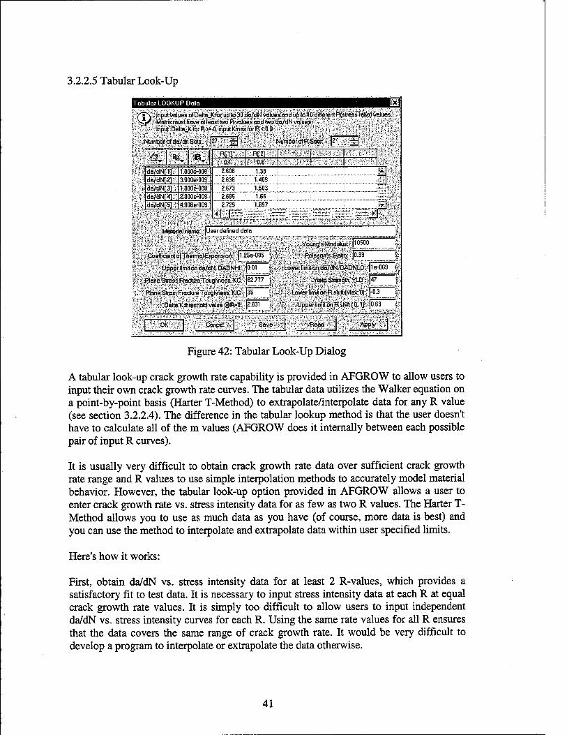
3.2.2.5 Tabular Look-Up
Tabular LOOKUP Data
iffi •Input valuesüifÖeltetiKforiup'to 30:da/dN vataesand upto;lfcdifferentß(streW^o)~;valuesÄ Matnxmustha/e et leasttwo Rvalues and two da/dN values « " •' Input Delta_K for R >• 0. input «max tor R < 0.0
Number of da/dn Sets »..£. Number of R Sets- |2 4 * •tfi. ■*T X R[1] R[2]
0.1 > '0.6 • da/dN[1] mmsm 2.606 1.38 ?M
1 dayaMt^fft 3;000&OÖ9; 2.636 1.409 £:;*
dä/dtsl[3] ;: lOOÖftOOSt 2.673 1.503 ; • do/dN[4] JEÖOOeWi 2.685 1.66 3? 1 ;da/dN[5]S M0ft008" 2.729 1.897
:i5£* ™ ~- ~J3 ► Z
,';r^™-~ -"w^- ™:,-*™t-
Matenal name: User defined data
Coefficient of Thermal Expansion: |1.25e-005
Young's Modulus: p0500
Poisson's Ratio- |0.33
UppeMimrt on da/dN. DADNHI- |0.01 Lowr limit on da/dN. DADNLO: le-009
■Plane-StressFractureToughn8ss.Ke:!!J62.777
;;Plan»StroinftaeturaToughness;.KIC:i;|35
' ' DettaKthreshold value @R-0: |2 831
YieldStrength.YLD;|^
Lower limit on R shift (Max: 0):' j-0.3
Upper limit ön R shift (0.1): 0.63
*OK:i; Cancel:5 ■iäave-i s^Readv I^PR'y*'
Figure 42: Tabular Look-Up Dialog
A tabular look-up crack growth rate capability is provided in APGROW to allow users to input their own crack growth rate curves. The tabular data utilizes the Walker equation on a point-by-point basis (Harter T-Method) to extrapolate/interpolate data for any R value (see section 3.2.2.4). The difference in the tabular lookup method is that the user doesn't have to calculate all of the m values (AFGROW does it internally between each possible pair of input R curves).
It is usually very difficult to obtain crack growth rate data over sufficient crack growth rate range and R values to use simple interpolation methods to accurately model material behavior. However, the tabular look-up option provided in AFGROW allows a user to enter crack growth rate vs. stress intensity data for as few as two R values. The Harter T- Method allows you to use as much data as you have (of course, more data is best) and you can use the method to interpolate and extrapolate data within user specified limits.
Here's how it works:
First, obtain da/dN vs. stress intensity data for at least 2 R-values, which provides a satisfactory fit to test data. It is necessary to input stress intensity data at each R at equal crack growth rate values. It is simply too difficult to allow users to input independent da/dN vs. stress intensity curves for each R. Using the same rate values for all R ensures that the data covers the same range of crack growth rate. It would be very difficult to develop a program to interpolate or extrapolate the data otherwise.
41

Set the values for the number of da/dN sets and R sets at the top of the dialog (see Figure 42) and enter the crack growth rate data in the matrix.
Enter the appropriate material property data for all fields in the lower half of the dialog box. AFGROW provides optional default material property values if the user wishes help with these parameters. The default values are merely typical properties for the materials listed. There is also a choice to add zeros to all of these data fields. This help is available by clicking on the default icon as shown in Figure 43 below:
\M fm\ da/cT da/c tfa/r;
Aluminum
Itanium
Steel j
^/cr:Allzero' ' :-
Figure 43: Tabular Look-Up Default Material Data
AFGROW includes the option to copy the crack growth data to the Windows clipboard to allow it to be pasted into another Windows application (i.e., Excel 7 or Excel 8). The entire table (excluding the parameters below the table), a single column, or a single row may be copied (see Figure 44). When copying a column or row, you must first click on the row or column to be copied.
,2].
Column 2 Row 2
3] 41
. Table f
Figure 44: Tabular Look-Up Copy Choices
Data that have been placed in the Windows clipboard from another Windows application (i.e. Excel 7 or Excel 8) may be pasted into AFGROW (see Figure 45). If the application is not in Excel format, be sure that the data are tab delimited in each row. When pasting a column or row, you must first click on the row or column where the data is to be pasted.
mi R[1] , ■^n}iv...t.
OOe-0,
OOe-0
Column "
00e-° Table
42

Figure 45: Tabular Look-Up Paste Choices
If Excel is used to create the crack growth rate data table, the required format is shown in Figure 46:
dadN/R 0.1 0.6 1.00E-09 2.606 1.38 3.00E-09 2.636 1.409 1.00E-08 2.673 1.503 2.00E-08 2.685 1.66 4.00E-08 2.729 1.897 6.00E-08 2.792 2.089 1.00E-07 2.954 2.355
Figure 46: Excel Spreadsheet Example for Crack Growth Rate Data
Error and Warning Checking:
Use the APPLY button to perform required error and warning checks on the data. Some tips are available for help dealing with the error messages.
When errors are detected in the user-input data, AFGROW will usually tell the user where the error is. If the error is in the crack growth rate data matrix, the coordinates of the location of the error are given. Errors that are found for extrapolated data may be difficult to debug. The easiest way to find the problem in these cases is to reduce the limits on R or crack growth rate (see Figure 42) to make them closer to the limits of the entered data until the error message(s) stop. The next step is to use the crack growth rate plotting capability in AFGROW to examine the data. It may be obvious where the error is after viewing the plots and scrolling between the upper and lower limits on R (Rio and Rhi).
The following error checks are performed:
• Positive R curves may NOT cross each other in the domain of the crack growth rate and R limits input by the user
• Negative R curves may NOT cross each other in the domain of the rate and R limits input by the user
• AK (or Kmax) values for a given R MUST increase with increasing rate • AK values for increasing positive R must decrease for increasing R • Kmax values for decreasing negative R must decrease for decreasing R • Kmax values for negative R values must be less than AK for R = 0.0 • Threshold AK value at R=0 must be in the range of AK for R=0 within the crack
growth rate limits input by the user • Kic must be less than Kc • RLO must be less than or equal to 0.0 • RHI must be greater than 0.0 AND less than 1.0
43

The following warning checks are performed:
• Data for negative R (Kmax) should be greater than the data (AK) at the same positive R
• Kmax values for negative R should be greater than data at R=0 when converted to AK (AK = Kmax*(l-R) - AFGROW will do this conversion internally)
Once the tabular data have been entered and applied (error checked), it may be saved in a file by clicking on the save button in the tabular look-up dialog. The format that is required for the tabular lookup data file [filename.lkp] is as follows (space delimited):
[No. of da/dN values] (2 min., 30 max.) [No. ofR values] (2 min., 10 max.)
m [R2].... [R^]
[da/dNj] [DK @ Rß [DK @ R2]... [DK @ R^]
[da/dN2] [DK @ R}] [DK @ R2]... [DK @ R^]
[da/dNnw] [DK @ Rj] [DK @ R2]... [DK @ R^]
[Rio] [K,c] [DADNLO] [Yield]
[Rhi] [Kc] [DADNHT] [THOLD]
[Poisson's ratio] [Coefficient of Thermal Expansion] [Modulus]
Remember that Kmax is required in place of AK for R < 0.0.
The following parameters are ONLY used in the analysis of bonded composite repairs:
Coefficient of Thermal Expansion: (Temperature)-l Used in the calculation of the thermal effect of patch cure temperature on the stress intensity factor of the patched metal.
Young's Modulus: (Stress) Used in the calculation of the stress intensity factor correction due to the presence of the bonded patch (also used in the initiation module).
Poisson's Ratio: (Non-Dimensional) Used in the calculation of the stress intensity factor correction due to the presence of the bonded patch.
44
The following parameters are used in the standard crack growth analysis:
DADNLO: (Length) Lower limit for da/dN extrapolation (uses log-log linear extrapolation based on the first two user input points for the appropriate R).
DADNHI: (Length) Upper limit for da/dN extrapolation (uses log-log linear extrapolation based on the last two user input points for the appropriate R).
Plane Stress Fracture Toughness (KC): (Stress, Length0-5) Value of Fracture Toughness to be used under pure plane stress conditions.
Plane Strain Fracture Toughness (KIC): (Stress, Length05) Value of Fracture Toughness to be used under pure plane strain conditions.
Delta K Threshold Value @ R=0: (Stress, Length0-5) Threshold stress intensity value at R=0 - no crack growth will be calculated when Delta K is below threshold for a given R value.
Yield Strength. (YLD): (Stress) Yield stress (0.2% strain) for the metal being analyzed.
Lower Limit on R Shift: (Non-Dimensional) R value below which no further R shifting is calculated.
Upper Limit on R Shift: (Non-Dimensional) R value above which no further R shifting is calculated.
Buttons:
OK: Accept the current (first does the error checking) choice and close the dialog box.
CANCEL: Cancel the dialog box.
SAVE: Save the current data to a user specified file.
READ: Read a previously saved file (*.lkp default extension).
APPLY: Apply the current input values to check for any errors.
45
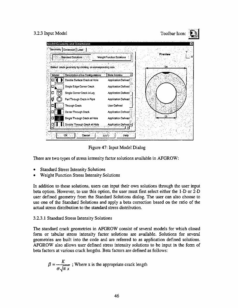
3.2.3 Input Model
Model Geometry and Dimensions
Geometry I Dimension | Load
-Standard Solutions.,: 'Weight Function Solutions
^Select crack geometry by clicking on corresponding icon
Model I Description of the Configurations | Beta Solution ''..•■, --.£]
°H> Double Surface Crack at Hole
Single Edge Comer Crack
Application Defined":
ot&: Application Defined/;:
CI HgH Single Corner Crack in Lug Application Defined
4© Part Through Crack in Pipe Application Defined;'
User Defined :% *tm Through Crack
°B0 Center Through Crock Application Defined.;:
QHH Single Through Crack at Hole Application Defined"-
Df-|Ij Double Through Crack at Hole Application Defined*!
-OK Cancel Apply Help
Toolbar Icon:
Preview .L*
Figure 47: Input Model Dialog
There are two types of stress intensity factor solutions available in AFGROW:
• Standard Stress Intensity Solutions • Weight Function Stress Intensity Solutions
In addition to these solutions, users can input their own solutions through the user input beta option. However, to use this option, the user must first select either the 1-D or 2-D user defined geometry from the Standard Solutions dialog. The user can also choose to use one of the Standard Solutions and apply a beta correction based on the ratio of the actual stress distribution to the standard stress distribution.
3.2.3.1 Standard Stress Intensity Solutions
The standard crack geometries in AFGROW consist of several models for which closed form or tabular stress intensity factor solutions are available. Solutions for several geometries are built into the code and are referred to as application defined solutions. AFGROW also allows user defined stress intensity solutions to be input in the form of beta factors at various crack lengths. Beta factors are defined as follows:
ß = K
CTJTTX ; Where x is the appropriate crack length
46

The crack length dimension in the thickness direction is the a-dimension and the crack length in the width direction is the c-dimension. Many of the standard stress intensity solutions in AFGROW use the popular Newman and Raju curve fit solutions to finite element results [16]. An angle, 0, is used in these equations to determine the stress intensity value for the crack growth dimensions (a, and c). This angle is defined as shown in Figure 48:
-*- Width
C - Dimension
Figure 48: Angle Used in Newman and Raju Solutions
The angle is measured from a line in the c-direction beginning at the crack origin. The closed-form Newman and Raju solutions do not necessarily match the finite element results at the free edges. Care was taken in AFGROW to use the angle for each crack dimension that tends to match the published finite element results near the free edges. The angles used in the Newman and Raju solutions for each crack dimension are documented in the following sections for models that use these solutions.
Application and user defined solutions are identified under the beta solution column in the geometry tab of the model dialog (see Figure 47). There are only two user-defined models among the standard solutions since AFGROW currently models only 1-D or 2-D cracks. The currently available standard solutions are described in the following sections.
3.2.3.1.1 Part Through-the-Thickness Crack (User Defined) I This model is used when a user has an existing stress intensity factor solution (in the form of a beta table) for any 2-D crack, which may be described with two length dimensions (2-D) to input in AFGROW.
The geometric beta values are NOT calculated by AFGROW, but are merely interpolated from a two-dimensional user-defined table of beta values. Users must supply beta values at various crack lengths so that the appropriate value at a given crack length may be interpolated. This model is shown as a corner cracked plate in the animation frame. The representation of the model is merely meant to indicate the two dimensional nature of the crack. It was not possible to create representations of all possible geometries that may be modeled using user defined beta factors
For the [a] crack length dimension: K = <7^7iäß(a)
For the [c] crack length dimension: K = o^ncß{c)
Al
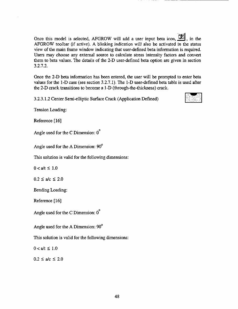
Once this model is selected, AFGROW will add a user input beta icon, ^1, in the AFGROW toolbar (if active). A blinking indication will also be activated in the status view of the main frame window indicating that user-defined beta information is required. Users may choose any external source to calculate stress intensity factors and convert them to beta values. The details of the 2-D user-defined beta option are given in section 3.2.7.2.
Once the 2-D beta information has been entered, the user will be prompted to enter beta values for the 1-D case (see section 3.2.7.1). The 1-D user-defined beta table is used after the 2-D crack transitions to become a 1-D (through-the-thickness) crack.
3.2.3.1.2 Center Semi-elliptic Surface Crack (Application Defined)
Tension Loading:
Reference [16]
0 Angle used for the C Dimension: 0
Angle used for the A Dimension: 90°
This solution is valid for the following dimensions:
0<a/t < 1.0
0.2 < a/c < 2.0
Bending Loading:
Reference [16]
o Angle used for the C Dimension: 0
Angle used for the A Dimension: 90°
This solution is valid for the following dimensions:
0<a/t < 1.0
0.2 < a/c < 2.0
48
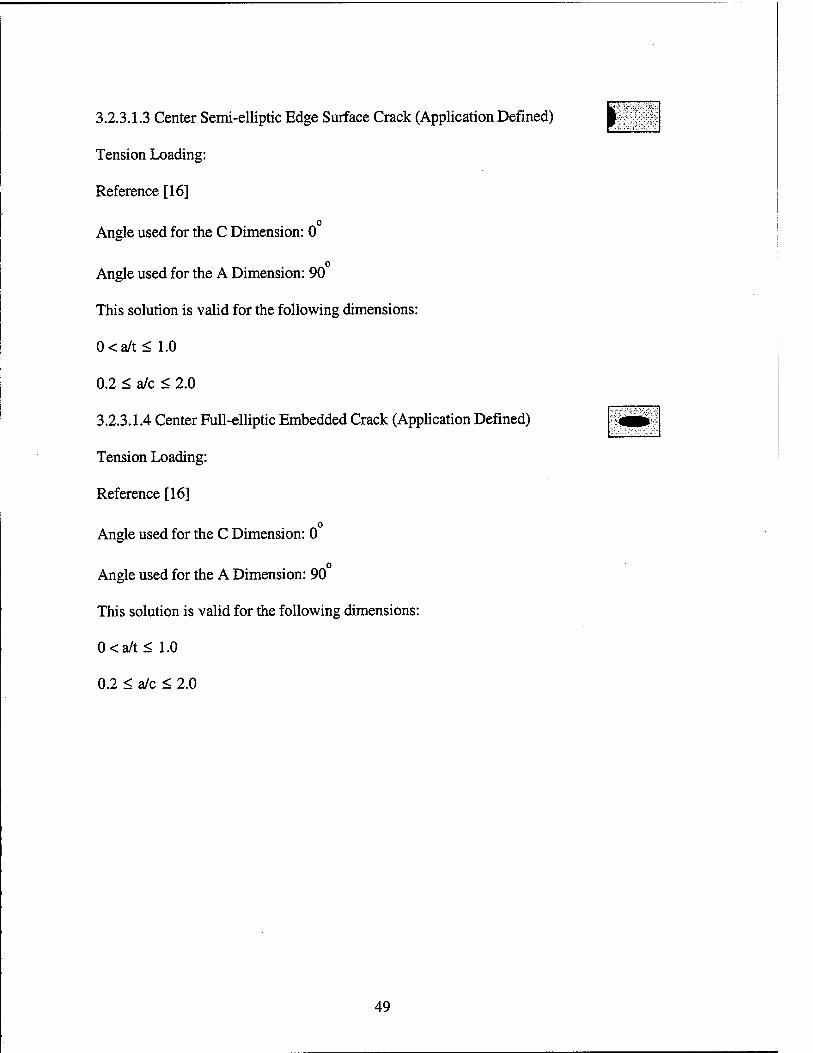
3.2.3.1.3 Center Semi-elliptic Edge Surface Crack (Application Defined) I
Tension Loading:
Reference [16]
o Angle used for the C Dimension: 0
0 Angle used for the A Dimension: 90
This solution is valid for the following dimensions:
0<a/t < 1.0
0.2 < a/c < 2.0
3.2.3.1.4 Center Full-elliptic Embedded Crack (Application Defined)
Tension Loading:
Reference [16]
o Angle used for the C Dimension: 0
o Angle used for the A Dimension: 90
This solution is valid for the following dimensions:
0<a/t < 1.0
0.2 < a/c < 2.0
49
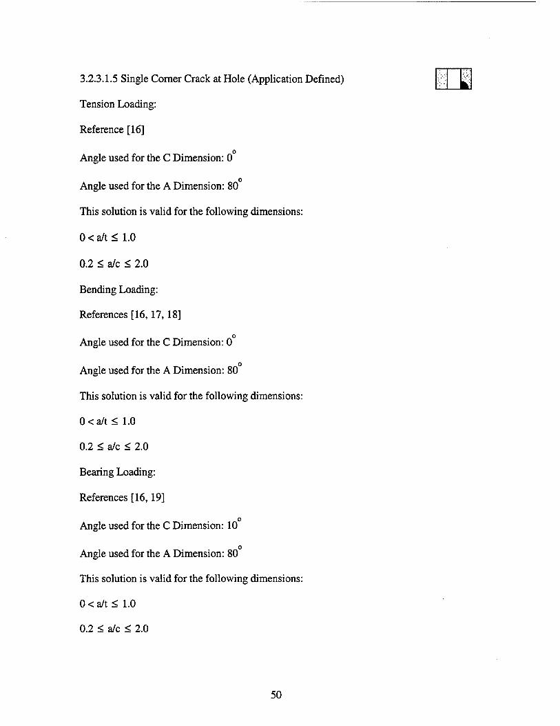
3.2.3.1.5 Single Corner Crack at Hole (Application Defined)
Tension Loading:
Reference [16]
o Angle used for the C Dimension: 0
o Angle used for the A Dimension: 80
This solution is valid for the following dimensions:
0<a/t< 1.0
0.2 < a/c < 2.0
Bending Loading:
References [16,17,18]
o Angle used for the C Dimension: 0
0 Angle used for the A Dimension: 80
This solution is valid for the following dimensions:
0<a/t < 1.0
0.2 < a/c < 2.0
Bearing Loading:
References [16,19]
o Angle used for the C Dimension: 10
0 Angle used for the A Dimension: 80
This solution is valid for the following dimensions:
0<a/t < 1.0
0.2 < a/c < 2.0
50
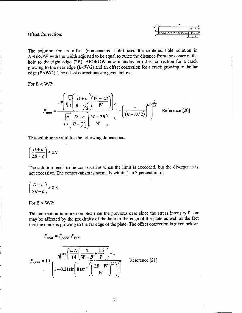
Offset Correction:
M _ »
: i"
. 0
The solution for an offset (non-centered hole) uses the centered hole solution in AFGROW with the width adjusted to be equal to twice the distance from the center of the hole to the right edge (2B). AFGROW now includes an offset correction for a crack growing to the near edge (B<W/2) and an offset correction for a crack growing to the far edge (B>W/2). The offset corrections are given below:
ForB<W/2:
sin D + c YW-2B^
F =■ B-9, W (
a ( \ D + c B-c,
2)
(W-2B^
) W
1-
D 12 Mi
(B-D/2) Reference [20]
This solution is valid for the following dimensions:
f D + c') 2B-c
<0.7
The solution tends to be conservative when the limit is exceeded, but the divergence is not excessive. The conservatism is normally within 1 to 3 percent until:
( D + c\ >0.8
2B-c
ForB>W/2:
This correction is more complex than the previous case since the stress intensity factor may be affected by the proximity of the hole to the edge of the plate as well as the fact that the crack is growing to the far edge of the plate. The offset correction is given below:
^offset ~ ^AHFB ^B/W
^AHFB — 1 +
1 + 0.21 sin 8 tan -i ((2B-WT]]
w
Reference [21]
51
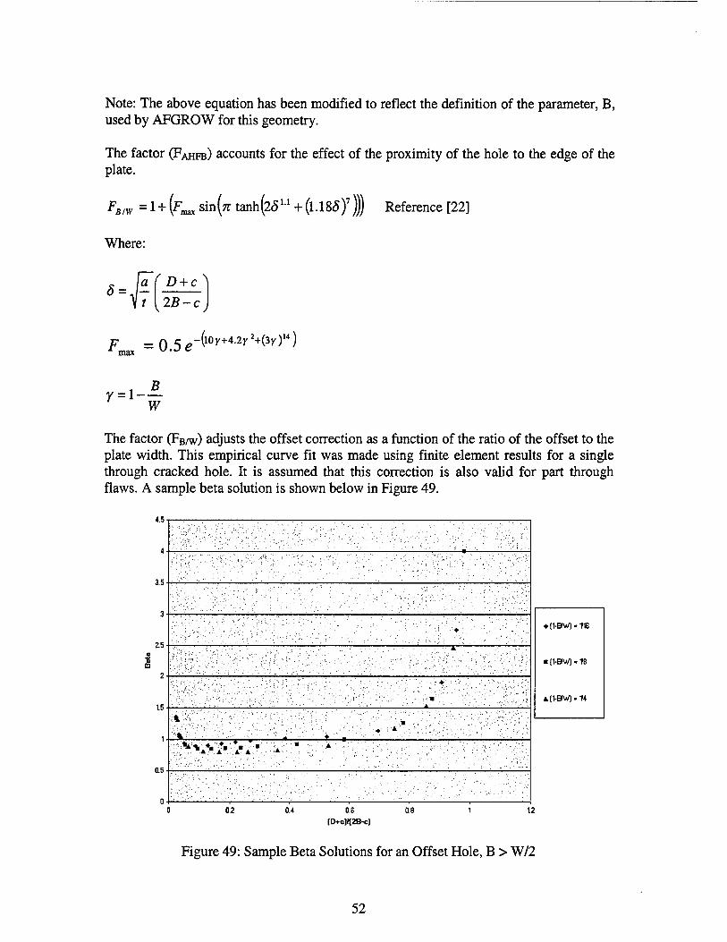
Note: The above equation has been modified to reflect the definition of the parameter, B, used by AFGROW for this geometry.
The factor (FAHFB) accounts for the effect of the proximity of the hole to the edge of the plate.
FB/W = 1 + (FM sin(^ tanh(25u + (l.lSS)7))) Reference [22]
Where:
S = . ( D + c\ 2B-c
F -n^-^r2^)14) 1 max v.J e
r = i- B_ W
The factor (FBAV) adjusts the offset correction as a function of the ratio of the offset to the plate width. This empirical curve fit was made using finite element results for a single through cracked hole. It is assumed that this correction is also valid for part through flaws. A sample beta solution is shown below in Figure 49.
4.5
3.5
Z5
15
0.5
, '.''::'.-:; ■ ■'■"•' "'.;''■':■ .-..■>■.■ '.'"'":.: :'■■':■' '''!■"■■■■■''''■.■."'':; ; ■''..''"■ "/.'^'V :'■■•■' .'■ '■■■■[ ..:-':f '.■'■: . :?''■-
■ (VBW) - K
A[VBW)-1f4
'.[:■' v--'/A/'- .y^:-. ■■'.;■■'' '■/:)■'KI- .'■', '.'.■'" .■ ■':■'■' '■''' •" ■.":•..,: ■■'•'.''' "•'♦ ■ ■'■'■ ■'■'■• '?.■■■' •'.■'■■■
"'.,:-.. ','-'', ' " A '
' ,■ -■' ' ' '. "■"'*■ ,■■>.■'..'■■ ' ' ♦'
";fö\',;;:. ..;;V":;'::::'''. ,-';':■/■. \..•:■:.:'.. :■'.]"> ■'. •■■■''.' '■' :L".:.: ■': :i '■':?[.■:>'''■" ■' 'l'^'■.'■'■'.'..'•".- :".'■ "■.:'.'""' ■*'■' :'.'V.''"i '..-''S.iO'/i:'
♦' ■ .;♦'
,'■"■':.".■'■■ '■■'■'■■ ■■:. v :'/v-v:;." :
>*»:■;■ ■■'■*■■"
.*■■
0.2 04 0.E |D*cW2B-c]
08 12
Figure 49: Sample Beta Solutions for an Offset Hole, B > W/2
52

3.2.3.1.6 Single Corner Crack at a Semi-Circular Notch (Application Defined)
Tension Loading:
Reference [23]
o Angle used for the C Dimension: 2.5
o Angle used for the A Dimension: 87
This solution is valid for the following dimensions:
0 < a/t < 1.0
0.2 < a/c < 2
1 < r/t < 2.0
(r+c)/w < 0.5
r/w=l/16 -+■ Kt = 3.17
Where, r is the notch radius
3.2.3.1.7 Single Surface Crack at Hole (Application Defined)
Tension Loading:
Reference [16]
o Angle used for the C Dimension: 0
0 Angle used for the A Dimension: 80
This solution is valid for the following dimensions:
0 < a/t < 1.0
0.2 < a/c < 2.0
I
53
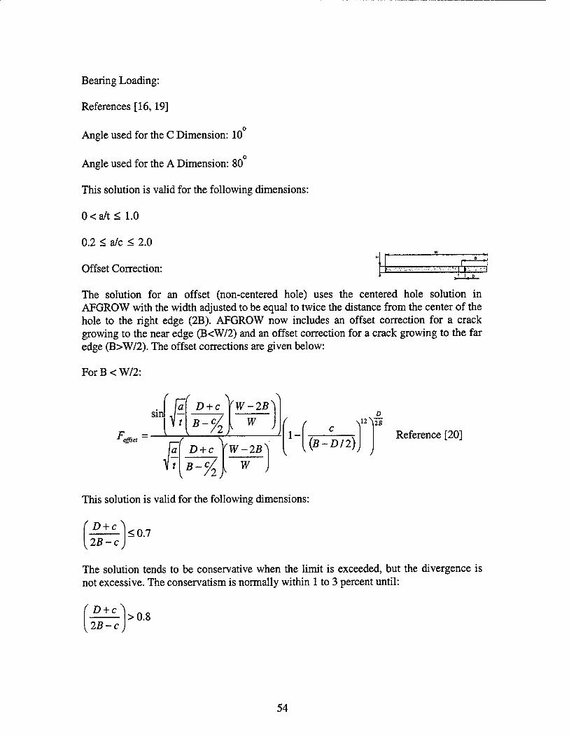
Bearing Loading:
References [16,19]
o Angle used for the C Dimension: 10
o Angle used for the A Dimension: 80
This solution is valid for the following dimensions:
0<a/t < 1.0
0.2 < a/c < 2.0
Offset Correction: w* The solution for an offset (non-centered hole) uses the centered hole solution in AFGROW with the width adjusted to be equal to twice the distance from the center of the hole to the right edge (2B). AFGROW now includes an offset correction for a crack growing to the near edge (B<W/2) and an offset correction for a crack growing to the far edge (B>W/2). The offset corrections are given below:
ForB<W/2:
sin (r-r V o D + c (W-2B^
F = B-9, W
D + c \w-2B^
( ( 1-
ß-c/, K '2) w
D
((B-D/2)) J Reference [20]
This solution is valid for the following dimensions:
( D + c^ 2B-c
<0.7
The solution tends to be conservative when the limit is exceeded, but the divergence is not excessive. The conservatism is normally within 1 to 3 percent until:
D + c 2B-c
\ >0.8
54

For B> W/2:
This correction is more complex than the previous case since the stress intensity factor may be affected by the proximity of the hole to the edge of the plate as well as the fact that the crack is growing to the far edge of the plate. The offset correction is given below:
^offset ~ ^AHFB ^B/W
sec 7lD f
F =1 + rAHFB x T
14 - + : 1.5 Y\
W-B B -1
l + 0.21sin 8 tan -i
^
'(2B-WT^ w
Reference [21]
Note: The above equation has been modified to reflect the definition of the parameter, B, used by AFGROW for this geometry.
The factor (FAHFB) accounts for the effect of the proximity of the hole to the edge of the plate.
FB/W = 1+ (F^ sin(?r tanh(2<5u + (l.l8<5)7))) Reference [22]
Where:
~ \a( D + c} S = J- 2B-c
Fm=0Se -(l0y+4.2y2+(3y)M)
w
The factor (FB/w) adjusts the offset correction as a function of the ratio of the offset to the plate width. This empirical curve fit was made using finite element results for a single through cracked hole. It is assumed that this correction is also valid for part through flaws. A sample beta solution is shown in Figure 49.
55
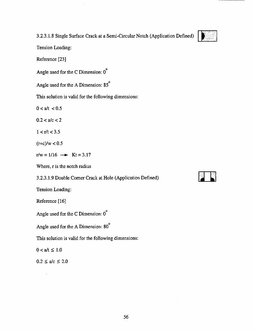
3.2.3.1.8 Single Surface Crack at a Semi-Circular Notch (Application Defined) ■;
Tension Loading:
Reference [23]
o Angle used for the C Dimension: 0
0 Angle used for the A Dimension: 85
This solution is valid for the following dimensions:
0<a/t <0.5
0.2 < a/c < 2
1 < r/t < 3.5
(r+c)/w < 0.5
r/w=l/16 -+■ Kt = 3.17
Where, r is the notch radius
3.2.3.1.9 Double Corner Crack at Hole (Application Defined) j|J
Tension Loading:
Reference [16]
o Angle used for the C Dimension: 0
o Angle used for the A Dimension: 80
This solution is valid for the following dimensions:
0<a/t < 1.0
0.2 < a/c < 2.0
56
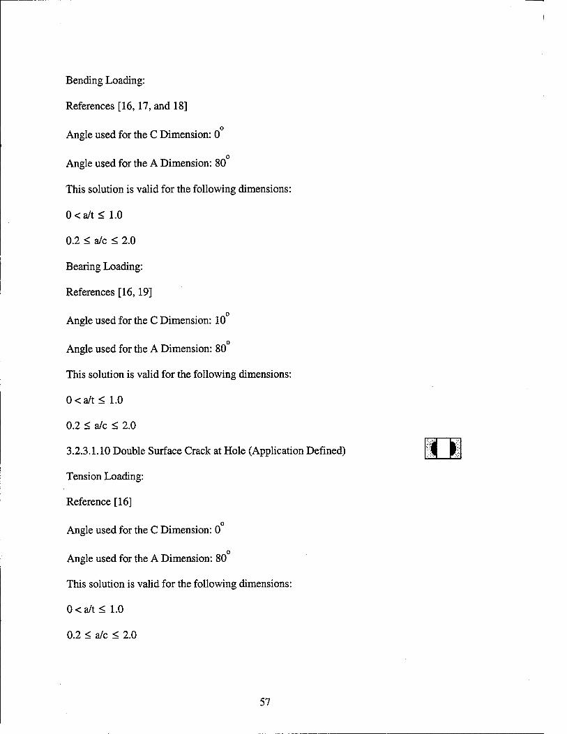
Bending Loading:
References [16,17, and 18]
o Angle used for the C Dimension: 0
o Angle used for the A Dimension: 80
This solution is valid for the following dimensions:
0 < a/t < 1.0
0.2 < a/c < 2.0
Bearing Loading:
References [16,19]
0 Angle used for the C Dimension: 10
0 Angle used for the A Dimension: 80
This solution is valid for the following dimensions:
0 < a/t < 1.0
0.2 < a/c < 2.0
3.2.3.1.10 Double Surface Crack at Hole (Application Defined) |j ||
Tension Loading:
Reference [16]
o Angle used for the C Dimension: 0
o Angle used for the A Dimension: 80
This solution is valid for the following dimensions:
0<a/t< 1.0
0.2 < a/c < 2.0
57
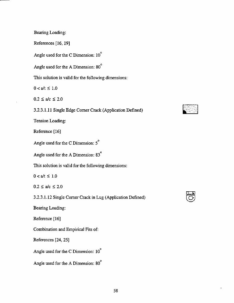
Bearing Loading:
References [16,19]
Angle used for the C Dimension: 10
0 Angle used for the A Dimension: 80
This solution is valid for the following dimensions:
0<a/t < 1.0
0.2 < a/c < 2.0
3.2.3.1.11 Single Edge Comer Crack (Application Defined)
Tension Loading:
Reference [16]
Angle used for the C Dimension: 5
Angle used for the A Dimension: 83
This solution is valid for the following dimensions:
0<a/t < 1.0
0.2 < a/c < 2.0 □ZE
3.2.3.1.12 Single Corner Crack in Lug (Application Defined) fo^j
Bearing Loading:
Reference [16]
Combination and Empirical Fits of:
References [24, 25]
Angle used for the C Dimension: 10
o Angle used for the A Dimension: 80
58

This solution is valid for the following dimensions:
0<a/t< 1.0
0.2 < a/c < 2.0
3.2.3.1.13 Part Through Crack in Pipe (Application Defined)
Tension Loading:
Reference [26]
0 Angle used for the C Dimension: 0
o Angle used for the A Dimension: 90
This solution is valid for the following dimensions:
0<a/t < 1.0
0.2 < a/c < 2.0
Bending Loading:
Reference [26]
o Angle used for the C Dimension: 0
0 Angle used for the A Dimension: 90
This solution is valid for the following dimensions:
0<a/t< 1.0
0.2 < a/c < 2.0
3.2.3.1.14 Through Crack (User Defined)
This model is used when a user has an existing stress intensity factor solution (in the form of a beta table) for any 1-D crack, which may be described with one length dimension (1- D) to input in AFGROW.
The geometric beta values are NOT calculated by AFGROW, but are merely interpolated from a one-dimensional user defined table of beta values. Users must supply beta values at various crack lengths so that the appropriate value at a given crack length may be interpolated. This model is shown as an edge cracked plate in the animation frame. The
59

representation of the model is merely meant to indicate the one-dimensional nature of the crack. It was not possible to create representations of all possible geometries that may be modeled using user defined beta factors
For the [c] crack length dimension: K = G^jncß(c)
Once this model is selected, AFGROW will add a user input beta icon, j±i|, in the AFGROW toolbar (if active). A blinking indication will also be activated in the status view of the main frame window indicating that user-defined beta information is required. Users may choose any external source to calculate stress intensity factors and convert them to beta values. Details of the through crack (1-D) user-defined beta option are given in section 3.2.7.1.
3.2.3.1.15 Center Through Crack (Application Defined)
Tension Loading:
/2CV _/2cV
■>.
Beta = 1.0-0.025 W
+ 0.06 w Jsecfr C/W)
Reference [27]
This solution is valid for the following dimensions:
0 < C/W < 0.5
This solution is within 0.1% for all crack lengths
Bending Loading:
2 Beta = — Beta (Tension)
3
It is important to be very clear that there is no way to provide a true solution for the out- of-plane bending case since the actual stress intensity value will vary through the thickness. The two thirds value is simply being used to provide a solution for the straight through crack that provides reasonable continuity with the bending solution for the c- dimension of the part-through (surface) crack. This solution is required to allow users to model bending for the surface crack case since the surface crack may transition to become a through crack. The most accurate way to model this case is to use an oblique through crack solution, which accounts for the changes in the stress intensity solution through the thickness. Unfortunately, no oblique internal crack solutions were found that are valid for the full range of crack shapes required. A partial oblique internal through crack solution was found [28] that could be used to provide a transition from a surface to a straight through crack. This option is available in the surface crack dialog (see section
60

3.2.3.1.2), but is NOT available for the through crack case. The oblique through crack solution does not cover the full range of possible oblique shapes. If this option is selected for the surface crack case, transition to a straight through crack will occur as soon as the crack shape exceeds the limits of the existing oblique solution.
Offset Correction:
The stress intensity solution for the offset internal through crack must be calculated at each crack tip. The offset case is non-symmetric, and the stress intensity values of each crack tip will be different. The offset parameter, B, is defined as the distance between the nearest plate edge and the center of the through crack. AFGROW measures this distance from the left edge of the plate and B must be less than one half of the plate width. Any offset case may be modeled in this manner. An offset crack on the right side of the plate will be on the left side if the plate is rotated 180 degrees.
The solution for the crack tip closest to the edge of the plate is:
Reference [29]
Beta = I sec l2J sin
( 4C ^ 2A e"
{ w j AC
IX eq
w
Where: A = -* B eg
Ceq = current half crack length Beq = current distance from the near plate edge to the crack center
The solution for the crack tip furthest from the plate edge is:
Reference [30]
Beta = 1 +
sec V 3nC„ V
2TCÄ + -, 2-T ■1
1 + 0.21 sin 8 tan -i
f „ JVC 71A-
x 0.9 Y
(W-Beq)
nC nl+ «L
(W-Beq) ))A
61
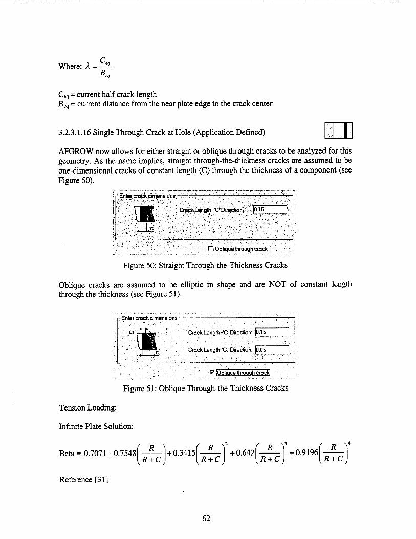
Where: X = — _£L B eg
Ceq = current half crack length Beq = current distance from the near plate edge to the crack center
3.2.3.1.16 Single Through Crack at Hole (Application Defined)
AFGROW now allows for either straight or oblique through cracks to be analyzed for this geometry. As the name implies, straight through-the-thickness cracks are assumed to be one-dimensional cracks of constant length (C) through the thickness of a component (see Figure 50).
^Entercrackdimensions, , j ; ■; ■.'■-.:■-•:
SjO.15 >i;i
IE V Obliqüeftröugh aäd< ,',:: ;
Figure 50: Straight Through-the-Thickness Cracks
Oblique cracks are assumed to be elliptic in shape and are NOT of constant length through the thickness (see Figure 51).
■'Enter crackdimensions-
Crack Length -'C Direction: |0.15
Crock Length-'Cf Direction: 0.05
'•'•.'.'•■'.• F Oblique through crack!
Figure 51: Oblique Through-the-Thickness Cracks
Tension Loading:
Infinite Plate Solution:
Beta= 0.7071 + 0.7548
Reference [31]
( R \ ( R \ + 0.3415 R + C R + C
+ 0.642 R } R + C
+ 0.9196 R V
R + C
62

Finite Width Correction:
Fw= , sec 7CR
W sec
(n (R + C/2) W-C
The finite width correction was taken from reference 16, Equation 46 with a/t set to 1.0.
This solution is valid for the following dimensions:
0 < C/R < infinite
R + C/2 W-C
<0.5
Bending Loading:
Infinite Plate Solution:
Reference [32]
Note: Equation 9 (single crack solution) was used from this reference - The actual beta value was obtained by dividing by yfn since the reference left that value out of the calculation of stress intensity.
(C/R + 2' C/R + l
A.5
FCF,
The factor, Fc, was added to correct equation 9 (which is a shear stress solution) to match the bending data provided in the above reference for a Poisson's ratio of 1/3. The error for any C/R was determined to be less than 1 percent for any C/R (for most values the error was MUCH less than 1 percent) according to the above reference. The difference between the data at Poisson's ratios of 1/3 and 1/4 is very small - other solutions use a correction for Poisson's ratio that is in great disagreement with this reference.
Fc = 0.9 + 0.083 (l - Kr0*46«™')+ 0.017 (l - 10-30(C/Ä))
63

Finite Width Correction:
Fw= Jsec (n_R
W
^ f sec
v
TcjR + C/2) W-C
The finite width correction was taken from reference 17, Equation 46 with a/t set to 1.0.
This solution is valid for the following dimensions:
0 < C/R < infinite
R + C/2 W-C
<0.5
Bearing Loading:
Beta = F4 * Fw
Infinite Plate Solution:
The infinite plate solution is interpolated from the tabular solution [19] shown below.
C/R 0.0 0.25 0.5 1.0 2.0 3.0 4.0 5.0 7.5 F4 0.95 0.6 0.429 0.286 0.177 0.13 0.107 0.095 0.095
Finite Width Correction:
Fw = . sec '7i(R + C)'\
W
Reference [33]
This solution is valid for the following dimensions:
0 < C/R < 7.5
(R + C)/W < 0.5
Oblique Through-the-Thickness Cracks
Dr. Scott Fawaz developed the finite element based oblique crack solutions for tension, bending, and bearing loading conditions [34, 35]. See Figure 51 for a description of the input requirements for the oblique crack.
64
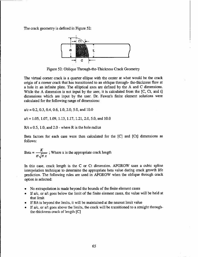
The crack geometry is defined in Figure 52:
i
Figure 52: Oblique Through-the-Thickness Crack Geometry
The virtual corner crack is a quarter ellipse with the center at what would be the crack origin of a corner crack that has transitioned to an oblique through- the-thickness flaw at a hole in an infinite plate. The elliptical axes are defined by the A and C dimensions. While the A dimension is not input by the user, it is calculated from the [C, Ct, and t] dimensions which are input by the user. Dr. Fawaz's finite element solutions were calculated for the following range of dimensions:
a/c = 0.2,0.3,0.4,0.6,1.0,2.0, 5.0, and 10.0
a/t = 1.05,1.07,1.09,1.13,1.17,1.21, 2.0, 5.0, and 10.0
R/t = 0.5,1.0, and 2.0 - where R is the hole radius
Beta factors for each case were then calculated for the [C] and [Ct] dimensions as follows:
Beta = —7= ; Where x is the appropriate crack length
In this case, crack length is the C or Ct dimension. AFGROW uses a cubic spline interpolation technique to determine the appropriate beta value during crack growth life prediction. The following rules are used in AFGROW when the oblique through crack option is selected:
• No extrapolation is made beyond the bounds of the finite element cases • If a/c, or a/t goes below the limit of the finite element cases, the value will be held at
that limit • If R/t is beyond the limits, it will be maintained at the nearest limit value • If a/c, or a/t goes above the limits, the crack will be transitioned to a straight through-
the-thickness crack of length [C]
65
Finite Width Correction:
Fw= , sec W
sec (n(R + C/2)}
W-C
The finite width correction was taken from Reference 17, Equation 46 with a/t set to 1.0.
This solution is valid for the following dimensions:
R + C/2 W-C
<0.5
The Fawaz solutions were calculated for the double cracked hole case and were corrected for the single crack case by the Shah correction as follows:
Beta (single crack) = Beta (double crack) *
Offset Correction:
lSR+n C *SR + 27t C
w —ii.-i. ■ ■ i I.»
I ■ ..... f=tr _ 0
The solution for an offset (non-centered hole) uses the centered hole solution in AFGROW with the width adjusted to be equal to twice the distance from the center of the hole to the right edge (2B). AFGROW now includes an offset correction for a crack growing to the near edge (B<W/2) and an offset correction for a crack growing to the far edge (B>W/2). The offset corrections are given below:
ForB<W/2:
sin (( ^
D + c
F =■ roffset
B-9, 1
'W-2By
W
\
D + c \w-2B} B-c/A W j
D
1- [ {(B-D/2)) J
This solution is valid for the following dimensions:
f D + c^ 2B-c
<0.7
Reference [20]
66
The solution tends to be conservative when the limit is exceeded, but the divergence is not excessive. The conservatism is normally within 1 to 3 percent until:
( D + c\ >0.8
2B-c
ForB>W/2:
This correction is more complex than the previous case since the stress intensity factor may be affected by the proximity of the hole to the edge of the plate as well as the fact that the crack is growing to the far edge of the plate. The offset correction is given below:
^offset = ^AHFB ^ BIW
(nD( 2 1.5?! sec
F =1 + 1 AHFB A ^
14 W-B B -1
/
l + 0.21sin 8 tan -i
V
flB-Wt9]) W
)JA
Reference [21]
Note: The above equation has been modified to reflect the definition of the parameter, B, used by AFGROW for this geometry.
The factor (FAHFB) accounts for the effect of the proximity of the hole to the edge of the plate.
FB/W = 1 + JF« sin(7T tanh(2<5u + (1.185)7))) Reference [22]
Where:
S = D + c 2B-c
F =0.5e"(10r+4-2/2+(3r)U)
w
The factor (FB/w) adjusts the offset correction as a function of the ratio of the offset to the plate width. This empirical curve fit was made using finite element results for a single through cracked hole. A sample beta solution is shown in Figure 49.
67

3.2.3.1.17 Double Through Crack at Hole (Application Defined) D AFGROW now allows for either straight or oblique through cracks to be analyzed for this geometry. As the name implies, straight through-the-thickness cracks are assumed to be one-dimensional cracks of constant length (C) through the thickness of a component (see Figure 50, section 3.2.3.1.16). Oblique cracks are assumed to be elliptic in shape and are NOT of constant length through the thickness (see Figure 51, section 3.2.3.1.16).
Tension Loading:
Infinite Plate Solution:
Beta = 0.5 ( 3.0-■
C ^ (
R + C 1.0 + 1.243
(
v 1.0-
c ^ 3\
R + C * -p
Reference [36]
Finite Width Correction:
Fw= , sec (nR\ (n(R + C)\
W sec
W
The finite width correction was taken from reference 16, Equation 46 with a/t set to 1.0.
This solution is valid for the following dimensions:
0 < C/R < infinite
R + C W
< 0.5
Bending Loading:
The double cracked hole solutions are corrected from the single-cracked solutions using the Shah Correction (with a/t set = 1.0)
Beta (double crack) = Beta (single crack) *
Infinite Plate Solution:
jSR + 2nC ' ZR + nC
Reference [32]
Note: Equation 9 (single crack solution) was used from this reference - The actual beta value was obtained by dividing by 4n since the reference left that value out of the calculation of stress intensity.
68
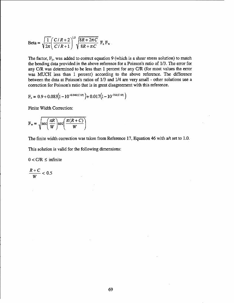
\2n\ C/R + l V SR + nC FCF„
The factor, Fc, was added to correct equation 9 (which is a shear stress solution) to match the bending data provided in the above reference for a Poisson's ratio of 1/3. The error for any C/R was determined to be less than 1 percent for any C/R (for most values the error was MUCH less than 1 percent) according to the above reference. The difference between the data at Poisson's ratios of 1/3 and 1/4 are very small - other solutions use a correction for Poisson's ratio that is in great disagreement with this reference.
Fc = 0.9 + 0.083(l - lo^-046^^)+ 0.017(l - 10-30(C/R))
Finite Width Correction:
Fw= Jsec (nR)
W sec n(R + C)
W
The finite width correction was taken from Reference 17, Equation 46 with a/t set to 1.0.
This solution is valid for the following dimensions:
0 < C/R < infinite
R + C W
< 0.5
69

Bearing Loading:
Beta = F3 * Fw
Infinite Plate Solution:
The infinite plate solution is interpolated from the tabular solution based on the following reference.
Reference [19]
C/R 0.0 0.25 0.5 0.75 1.0 2.0 3.0 4.0 5.0 7.5 10.0 F3 0.84 0.575 0.455 0.380 0.325 0.22 0.173 0.143 0.125 0.1 0.1
Finite Width Correction:
Fw= Jsec (n(R + C)']
W
Reference [33]
This solution is valid for the following dimensions:
0 < C/R < 10
(R + Q/W < 0.5
Oblique Through-the-Thickness Cracks:
Dr. Scott Fawaz developed the finite element based oblique crack solutions for tension, bending, and bearing loading conditions [34,35].
The virtual corner crack is a quarter ellipse with the center at what would be the crack origin of a corner crack that has transitioned to an oblique through-the-thickness flaw at a hole in an infinite plate (see Figure 52, section 3.2.3.1.16). The elliptical axes are defined by the A and C dimensions. While the A dimension is not input by the user, it is calculated from the [C, Ct, and t] dimensions which are input by the user. Dr. Fawaz's finite element solutions were calculated for the following range of dimensions:
a/c = 0.2,0.3,0.4,0.6,1.0,2.0, 5.0, and 10.0
a/t = 1.05,1.07,1.09,1.13,1.17,1.21,2.0,5.0, and 10.0
R/t = 0.5,1.0, and 2.0 - where R is the hole radius
70

Beta factors for each case were then calculated for the [C] and [Ct] dimensions as follows:
Beta = —j= ; Where x is the appropriate crack length G^TtX
In this case, crack length is the C or Ct dimension. AFGRÖW uses a cubic spline interpolation technique to determine the appropriate beta value during crack growth life prediction. The following rules are used in AFGROW when the oblique through crack option is selected:
• No extrapolation is made beyond the bounds of the finite element cases • If a/c, or a/t goes below the limit of the finite element cases, the value will be held at
that limit • If R/t is beyond the limits, it will be maintained at the nearest limit value • If a/c, or a/t goes above the limits, the crack will be transitioned to a straight through-
the-thickness crack of length [C]
Finite Width Correction:
f, Fw= Jsec
nR\ (n(R + C)}
KW J sec
W
The finite width correction was taken from reference 16, Equation 46 with a/t set to 1.0.
This solution is valid for the following dimensions:
R + C _ . < 0.5
W
3.2.3.1.18 Through Crack at a Semi-Circular Notch (Application Defined)
Tension Loading:
Reference [23]
This solution is valid for the following dimensions:
(r+c)/w < 0.8
r/w=l/16 —► Kt = 3.17
Where, r is the notch radius
71
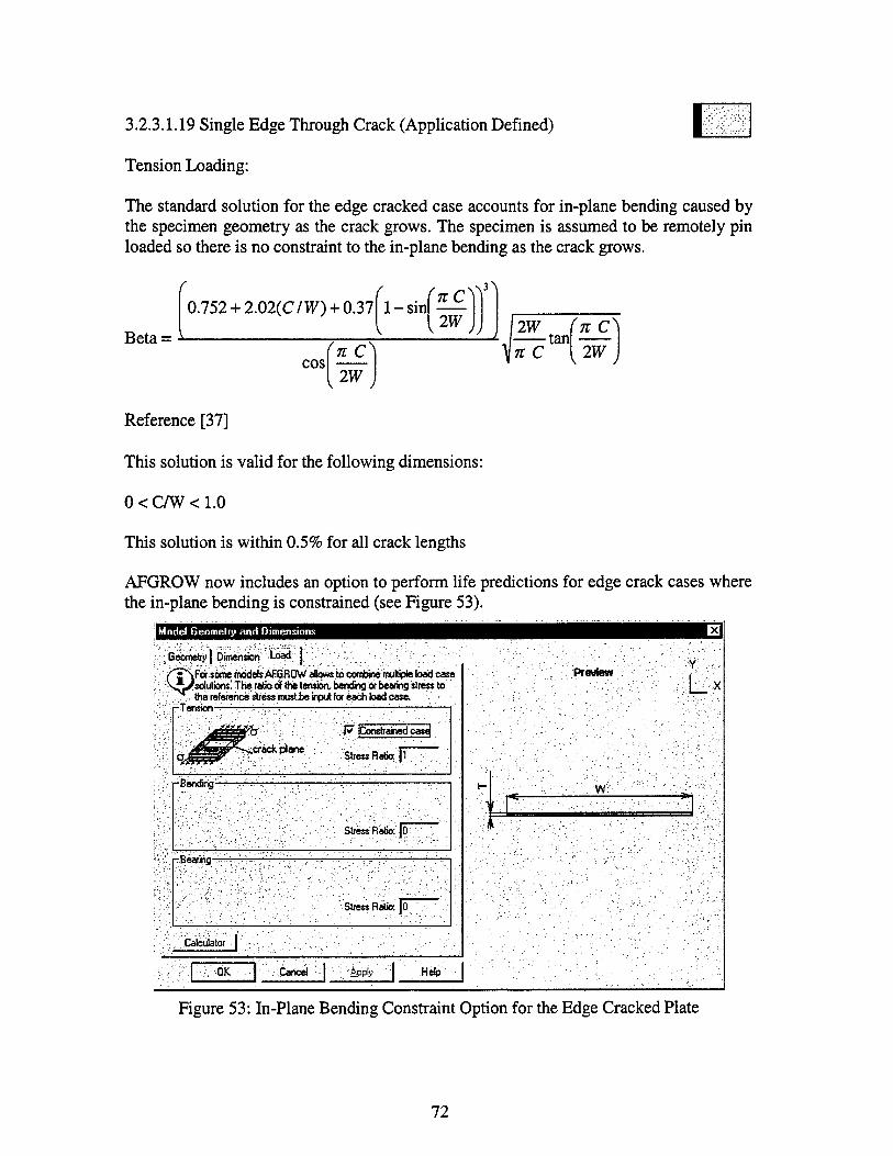
[ 3.2.3.1.19 Single Edge Through Crack (Application Defined)
Tension Loading:
The standard solution for the edge cracked case accounts for in-plane bending caused by the specimen geometry as the crack grows. The specimen is assumed to be remotely pin loaded so there is no constraint to the in-plane bending as the crack grows.
(
Beta:
/ 0.752 + 2.02(C/W) + 0.37 1-sin
fnC\)3] 2W ))
cos 2W
2W (n C^ ■tan
\n C 2W
Reference [37]
This solution is valid for the following dimensions:
0 < C/W < 1.0
This solution is within 0.5% for all crack lengths
AFGROW now includes an option to perform life predictions for edge crack cases where the in-plane bending is constrained (see Figure 53).
Model Geometry and Dimensions
Geometry] Dimension Load
m Fa sörra models ÄHGROWaBom to 'sorutions! The ratio of the tension, bending or bearing stress to theTeference stress müslbe input for each load case,
r Tension -—--■.,.■■—— : !
•p\ jConstrained casej
Stress Ratio: |1
OK | Cancel Apply Help
Preview
w:
Figure 53: In-Plane Bending Constraint Option for the Edge Cracked Plate
72
To constrain (eliminate) the in-plane bending contribution from the single edge cracked plate, select the option for the constrained case in the load tab for the edge crack model as shown in Figure 53. The constrained solution was determined from numerous finite element models using FRANC2D/L [38].
The easiest way to eliminate in-plane bending from the edge crack case is to apply a uniform displacement to the finite element model. This method can be used to determine the stress intensity factor for a specific case. To be applicable to all edge crack cases, this solution should be in the form of a beta factor table.
Beta = —-. ; Where c is the crack length a^jn c
If the stress intensity factor is known for a given edge crack case, the beta factor may be determined if the remote applied stress, a, is known. The remote stress for the uniform displacement model can be extracted from the finite element model for relatively short cracks. When longer crack lengths are modeled it becomes more difficult to determine the equivalent remote stress since the longer cracks cause large changes in the internal stress distribution. Applying a uniformly distributed unit stress to the plate and constraining the displacement (normal to the applied stress) of the mid-plane nodes in the upper and lower portions of the plate model solved this problem. It was important to constrain only the mid-plane nodes to maintain a uniform stress field through the plate width. The nodes in the area of the crack plane were NOT constrained. The beta values obtained using this approach were accurate within 0.1 percent of the uniform displacement method for the shorter crack lengths (where they could be compared). In addition, the stress distributions were in very good agreement for the long crack cases.
The beta solution for an edge crack in a semi-infinite plate is known to be equal to 1.122. This is true for both the constrained and unconstrained cases. The solution for the finite width cases is:
Beta = 1.122 * Fw; Where, Fw is the finite width correction
73
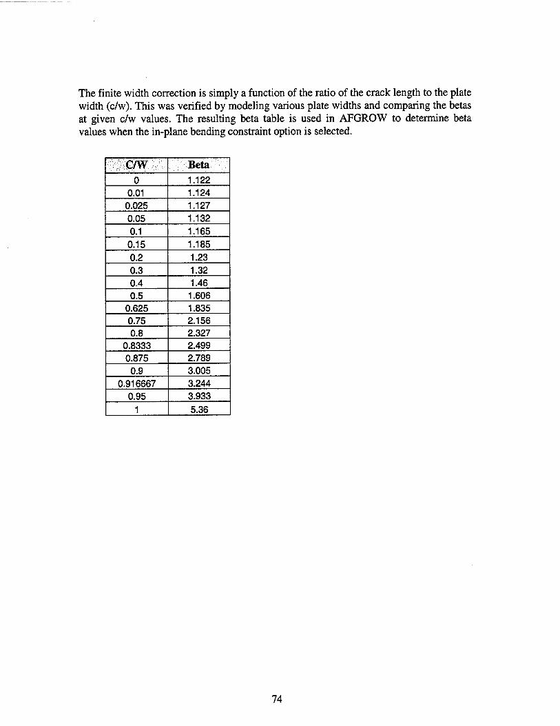
The finite width correction is simply a function of the ratio of the crack length to the plate width (c/w). This was verified by modeling various plate widths and comparing the betas at given c/w values. The resulting beta table is used in AFGROW to determine beta values when the in-plane bending constraint option is selected.
C/W Beta 0 1.122
0.01 1.124 0.025 1.127 0.05 1.132 0.1 1.165
0.15 1.185 0.2 1.23 0.3 1.32 0.4 1.46 0.5 1.606
0.625 1.835 0.75 2.156 0.8 2.327
0.8333 2.499 0.875 2.789
0.9 3.005 0.916667 3.244
0.95 3.933 1 5.36
74

3.2.3.1.20 Double Edge Through Crack (Application Defined)
Tension Loading:
□ Beta = 1.0 + 0.122COS4 (nCX\ lw_ -tan
(nC\ W y YY J
Reference [39]
This solution is valid for the following dimensions:
0 < C/W < 0.5
This solution is within 0.5% for all crack lengths
3.2.3.1.21 WOL/CT Specimen (Application Defined) I Note: The loading for this geometry is applied as pin loads through bolt holes in the specimen. Therefore, the input tension (stress) value is not really a stress value, but is LOAD. When using this geometry, the user must input the applied LOAD instead of stress. The diagram in the loads tab indicates a remote stress input, but this is because all other geometries use remote stress as the input for the tension case. This geometry is an exception to that rule.
Tension Loading:
Reference [39]
This solution is valid for the following dimensions:
0.2 < C/W <= 0.975
This solution is within 0.5% for all crack lengths in the range above.
75

3.2.3.1.22 Single Edge Crack in Lug (Application Defined) UL=JJ
Bearing Loading:
Combination and Empirical Fits of:
References [24, 25]
3.2.3.1.23 Rod (Application Defined)
Tension Loading:
Reference [41]
Bending Loading:
Reference [41]
3.2.3.1.24 Through Crack in Pipe (Application Defined)
Tension Loading:
Reference [42]
Bending Loading:
Reference [42]
76

3.2.3.2 Weight Function Stress Intensity Solutions
The weight function solutions [7] in AFGROW were provided under sub-contract to AS&M by Prof. G. Glinka, University of Waterloo, CA. Professor Glinka's solutions were translated to the C/C++ language and adapted for use in AFGROW.
3.2.3.2.1 Center Semi-Elliptical Surface Crack (Glinka's Weight Function)
This solution is valid for the following dimensions:
0 < a/t < 0.8
0 < a/c < 2.0
3.2.3.2.2 Single Corner Crack (Glinka's Weight Function)
This solution is valid for the following dimensions:
0 < a/t < 0.8
0.2 < a/c < 1.0
3.2.3.2.3 Internal Axial Crack in Thick Pipe (Glinka's Weight Function)
This solution is valid for the following dimensions:
1.1 < Ro/Rj < 2.0 ; Where R0: Outside Pipe Radius, Rj: Inside Pipe Radius
0 < a/t < 0.8
0.2 < a/c < 1.0
3.2.3.2.4 External Axial Crack in Thick Pipe (Glinka's Weight Function)
This solution is valid for the following dimensions:
1.1 < RQ/R < 2.0 ; Where R0: Outside Pipe Radius, Ri: Inside Pipe Radius
0 < a/t < 1.0
0.2 < a/c < 1.0
I
@
77
□
o
3.2.3.2.5 Center Through Crack (Glinka's Weight Function)
This solution is valid for the following dimensions:
0 < c/w < 0.45
3.2.3.2.6 Single Edge Through Crack (Glinka's Weight Function) |
This solution is valid for the following dimensions:
0 < c/w < 0.9
3.2.3.2.7 Double Edge Through Crack (Glinka's Weight Function)
This solution is valid for the following dimensions:
0 < c/w < 0.45
3.2.3.2.8 Radial Edge Crack in Disc (Glinka's Weight Function)
This solution is valid for the following dimensions:
0 < c/Dia. < 0.9
3.2.3.2.9 Axial Through Crack in Thick Pipe (Glinka's Weight Function)
This solution is valid for the following dimensions:
l.l<=Ro/Ri<=2.0
0 < c/w < 0.45
3.2.3.3 Using the Weight Function Solutions
The 2-D solutions currently allow the input stress field to vary in the one direction only (currently the distribution in the thickness (y) direction). The details of the stress field input are given in the stress distribution dialog. When the part through the thickness cracks transition to become through-the-thickness cracks, the model is automatically changed to the appropriate 1-D case and the applicable stress distribution is used to continue the life prediction. The stress distribution in the width (x) direction is always used for 1-D cases. Certain Tips and Tricks are available to provide additional guidance in the use of the weight function solutions.
78

3.2.3.3.1 Weight Function Stress Distribution
The decision whether to normalize the input stress distribution is really a personal preference as long as you have a clear understanding of the relationship between the input spectrum, stress multiplication factor, and the stress distribution you plan to use. The main thing to remember is that all three values are multiplied together by AFGROW to determine the stress values at each point where you input stress (or load).
For example, to simulate a double-cracked open hole with a remote gross stress (P/(W*t)) of 14 ksi, R = 0, initial crack size = 0.07 in, (from hole), the following was done:
• A normalized spectrum was used - Max Stress =1.0 • Stress Multiplication Factor = 14 • Finite element results (FRANC2D) provided un-flawed Kt vs. crack length in the
crack plane. • Center cracked weight function model was chosen based on geometric similarity • Open hole (0.5 in. dia.) modeled by a stress free zone • Initial half crack length = 0.25 (radius) + 0.07 = 0.32 in.
The stress distribution dialog is shown in Figure 54: Model Geometry and Dimensions
Geometoy| Dimension} Load Stress Distribution ]
W^\ AFGROWaseS''uncrack8dl:norrnali2ed'StressdistributionS()0in . JVsir-:.-. prospective'Cxrackplane and S(y) in »W1o calculate stress -
inteneitytactors by WeightFundions. . ?-;•<-S(4isusedfor1hroughcrack.calculaSonandSMfor.partthrough. ■-;-
ttis recdmendedtonormafeSfc)" sand Sfy) lableby. slressvalue In -r- the crackongrn S(u.B)
llK survide acbye Stable
J] by |0
'A . ' . : " •' . '
. Save | Read |
.*/'Cut*; | ;jPasfe:|
" Undo [
■*iumberof:Sefc 1« .. ±1 :;Set <• JX . Ki- l:aS(x)-5 ß S0.-4S ll
0.249 ! 0 ; 0 sir--;'. ^■■;
2 0.25 : 3.036 :~: <';'3-K\? 0.3 2.3064
~AH- "i- 0.35 . 1.5766 -•') i.5,;.: > 0.5 : 1.251 -*l "- ".. r
<-0K';: I . Eancel • iiäPPly ■■: ijHelp;';
^Pr«vi«wi :L'x
Figure 54: Weight Function Stress Distribution Dialog
AFGROW provides a tool to allow the stress values to be divided by a given number. This is especially helpful in cases where the user wants to normalize the stress values.
Since there is no weight function solution for a double cracked hole, the center-cracked case was used with a stress free area where the hole would have been located. A total of ten points were used to characterize the unflawed stress distribution in the crack plane.
79

The input distribution is shown in the stress distribution dialog. AFGROW accepts a maximum of 25 points to define the stress distribution. The points do not have to be equally spaced, but should be spaced such that linear interpolation between points adequately matches the desired distribution.
In order to judge the effectiveness of this approximate solution, a comparison of life prediction analyses was made between this solution and the standard double cracked hole solution (see Figure 55).
Double Through Cracked Hole Ma» Gross Stress = 14 Ksi, R = 0. W = 4.0 in., Dia. = 0.5 in.
2024-T3 Aluminum Tabular Data
5000 10000 15000 20000 25000
Cycles
- AFGROW - Standard Solution — —AFGROW - Glinka's Weight Funetion(Ccnter Crack)
Figure 55: Comparison Between Weight Function and Standard Solutions
The weight function solution resulted in an excellent agreement in life to a certain crack length. This comparison is very sensitive to small changes in stress intensity. Hence, this approximation is excellent to a crack length of approximately 0.5 inches.
3.2.3.3.2 Weight Function Tips and Tricks
Choose the Appropriate Weight Function Model. Try to choose the model that is geometrically CLOSEST to the problem being approximated.
The current 2-D weight function solutions in AFGROW only permit the input stress distribution to vary in a single direction. Prof. Glinka's solutions for part-through cases can be adjusted to switch dimensions. At this time, only the single corner and surface crack models are available. Future releases are planned which will include additional models.
80

If a through crack at an edge notched specimen is being modeled, use the edge crack model, determine the unflawed stress distribution, and model the notch depth as a stress free area as was done in the example given above
Additional tips or tricks will be provided as more experience is gained working with the solutions.
3.2.3.3.3 Weight Function Verification
Comparisons between weight function and available closed-form stress intensity solutions have been made to aid in the verification of the weight function solutions. Selected weight function stress intensity models, provided by Prof. Glinka, have been compared to existing closed form solutions to demonstrate the accuracy of the weight function solutions. A copy of the stress distribution dialog is provided for each case. The results are shown below in Figure 56 and Figure 57:
0.5
Center Cracked Plate Uniform Remote Stress
1 1.5
Crack Length
-AFGROW - Standard Solution, W=4.0 in. — AFGROW - Glinka'; Weight Function, W=4.0 in.
Figure 56: Center Crack Under Uniform Tensile Loading
81
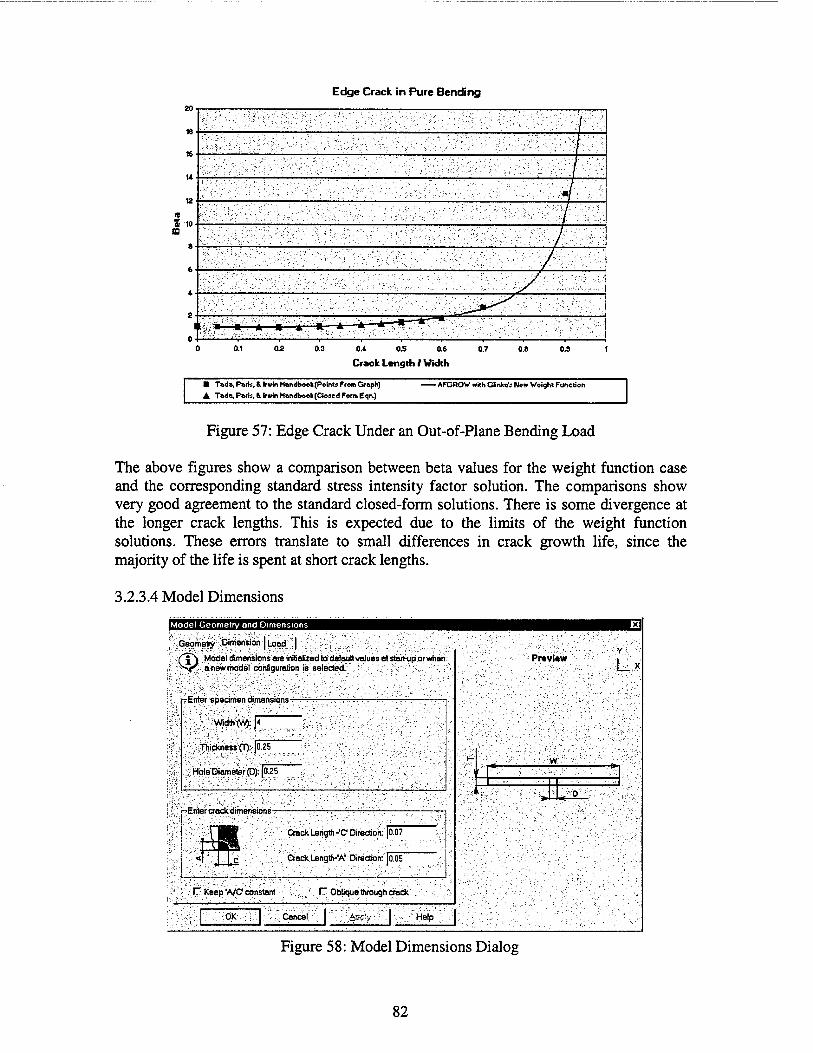
Edge Crack in Pure Bending
5 10 03
0.1 0.4 0.5 0.6
Crack Length / Width
0.7 0.8 0.8
■ Tads, Paris, 8. Irwin Handbook(Points From Graph) AFGP.OW with Glinka's New Weight Function A Tad«. Paris, 8. Irwin Handbook(Clo»d Form Eqn.)
Figure 57: Edge Crack Under an Out-of-Plane Bending Load
The above figures show a comparison between beta values for the weight function case and the corresponding standard stress intensity factor solution. The comparisons show very good agreement to the standard closed-form solutions. There is some divergence at the longer crack lengths. This is expected due to the limits of the weight function solutions. These errors translate to small differences in crack growth life, since the majority of the life is spent at short crack lengths.
3.2.3.4 Model Dimensions
Model Geometry and Dimensions
■ :Gaom8try -Pimension 1 Load I .' ' '/
/"jN Model dimensions are initialized to default values at start-up orwhen ,:^>r anewmode! configuration is selected.
Enter specimen dimensions-
/; <Wid1h(W):j4~
T>ickness'fr): p-25
Hole Diameter (D): (0.25
r-Enter crock dimensions-
Crack Length ->C direction." JO.07
'. GrackLength-'A' Direction:''|Ö!ÖT"
I- Keep 'A/C constant f~ Oblique ihrough crack
; Preview ■;.YJ.
V* r" ~.v. ■ .') '■ ':'r,:*yy :':'jv' •■•■;■■■ ■:'■,
1, '■■'- >. «:°...
-OK- . Cancel'' Applv, Help
Figure 58: Model Dimensions Dialog
82
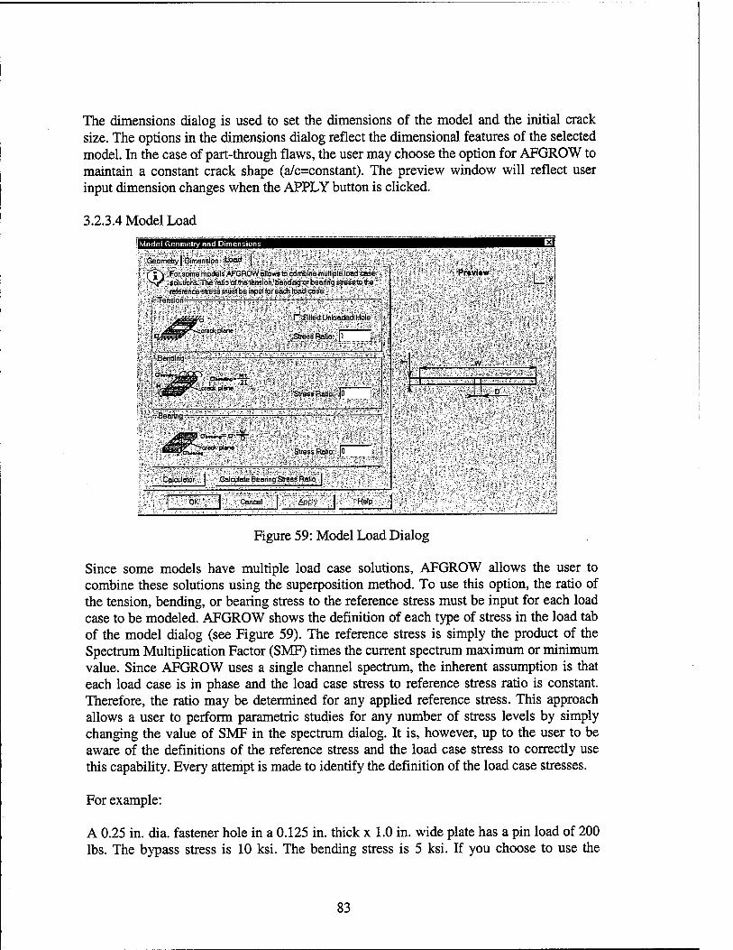
The dimensions dialog is used to set the dimensions of the model and the initial crack size. The options in the dimensions dialog reflect the dimensional features of the selected model. In the case of part-through flaws, the user may choose the option for AFGROW to maintain a constant crack shape (a/c=constant). The preview window will reflect user input dimension changes when the APPLY button is clicked.
3.2.3.4 Model Load Model Geometry and Dimensions
Geometry | Dimension toad | . ' ^, , ^
**'(f"\ ^«.«om8'mod^*raR0W^owstocoRi6toeT«ulliple.taad««»; i*r 5*4/1 /solutränscirhe'rafibätjfthBlensionvbendingar bearing stresslothe'
reference stress must be input for each toad case. -Tension-
r,f?illedUnloadedHble:S
ftStress'BaSd:!.!
~.Bending-
^.crack'ptanct Stress Ratio: (o
SBearirigs
~crack plane Wi
•Stress RaSo: JO
' Calculator' j 'Galculate'Beanng* Stress Ratio";)'
Pr«viaw Lx
V't-
t'm; /Cancel. iiÄ':: 'Help-
Figure 59: Model Load Dialog
Since some models have multiple load case solutions, AFGROW allows the user to combine these solutions using the superposition method. To use this option, the ratio of the tension, bending, or bearing stress to the reference stress must be input for each load case to be modeled. AFGROW shows the definition of each type of stress in the load tab of the model dialog (see Figure 59). The reference stress is simply the product of the Spectrum Multiplication Factor (SMF) times the current spectrum maximum or minimum value. Since AFGROW uses a single channel spectrum, the inherent assumption is that each load case is in phase and the load case stress to reference stress ratio is constant. Therefore, the ratio may be determined for any applied reference stress. This approach allows a user to perform parametric studies for any number of stress levels by simply changing the value of SMF in the spectrum dialog. It is, however, up to the user to be aware of the definitions of the reference stress and the load case stress to correctly use this capability. Every attempt is made to identify the definition of the load case stresses.
For example:
A 0.25 in. dia. fastener hole in a 0.125 in. thick x 1.0 in. wide plate has a pin load of 200 lbs. The bypass stress is 10 ksi. The bending stress is 5 ksi. If you choose to use the
83

remotely applied gross stress (bypass stress + bending stress + pin load/(width * thickness)) as the reference stress, then the total gross remote stress is:
10 ksi + 5 ksi + 200/(0.125 * 1.0) * 0.001 = 16.6 ksi
Therefore,
The tensile stress ratio is: 10/16.6 = 0.6024
The bending stress ratio is: 5/16.6 = 0.3012
The bearing stress ratio is: (200/(0.25 * 0.125) * 0.001)/16.6 = 0.3855
These ratios have nothing to do with a "percent load transfer." There is no limitation that these ratios add to 1.0. Depending on the situation, the ratios can easily be much greater than 1.0. The reason the ratios do not add to 1.0 in this case is because the stress intensity solution for the bearing load case is based on bearing stress instead of gross stress. It is necessary to "fool" AFGROW to use a common reference stress. It is generally a good practice to use gross stress as the reference since the majority of models use gross stress and it will usually minimize any necessary conversions.
A calculator option is available to aid the user in making the appropriate calculations.
Note: For models with tension and bearing load solutions, AFGROW includes an option to calculate the bearing stress ratio automatically based on the tension stress ratio using the following relationship:
Bearing Stress Ratio = (1 - Tension Stress Ratio) * W/Dia.
This assumes that the input stress spectrum and spectrum multiplication factor are referenced to the remote tensile gross stress. In addition, this option will not function in cases where a non-zero bending stress ratio is applied. If a bending stress component is included, the user must calculate each stress ratio as shown in the example at the top of this page.
84
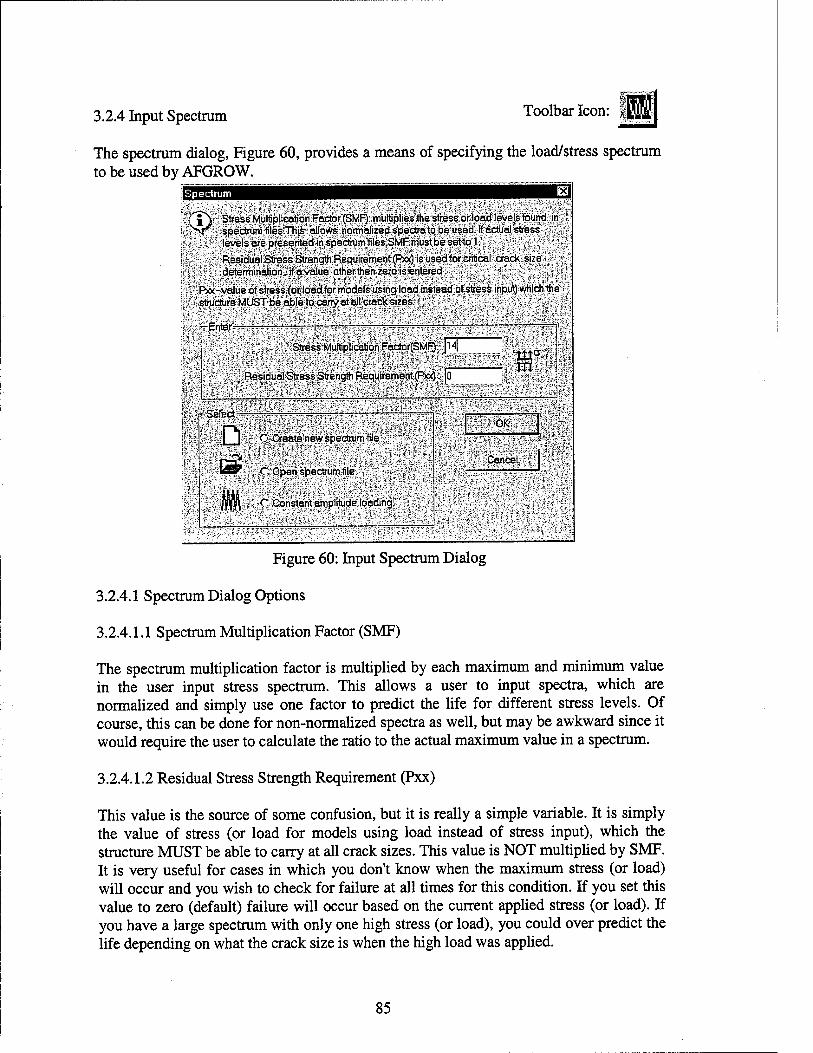
3.2.4 Input Spectrum Toolbar Icon:
The spectrum dialog, Figure 60, provides a means of specifying the load/stress spectrum to be used by AFGROW.
Spectrum
{J\ Stress Multiplication Factor (SMF): multiplies the-stress orload levels found in 3^jr spectrum files.This allows normalized spectra to be used. If actual stress ■ . levelsarepreserrtedinspectrurnfiles.SMFmustbesettol.
" Residual Stress Strength Requirement.^») is used for critical crack size determination, if a value otherthen zero is entered.
Pxx-value of stress (or load for models using load instead of stress input) which the ' structure MUST be able to carry at all crack sizes.
•Enter ■■ ■■ ■■ ■ ——: — ,
Stress Multiplication FactorfSMF): |l4|
Residual Stress Strength Requirement (Pxx): 0
-Select —
D r Create new spectrum file'
GS C Operi spectrum file
M ft r Constant amplitude loading
W§Si
Cancel
Figure 60: Input Spectrum Dialog
3.2.4.1 Spectrum Dialog Options
3.2.4.1.1 Spectrum Multiplication Factor (SMF)
The spectrum multiplication factor is multiplied by each maximum and minimum value in the user input stress spectrum. This allows a user to input spectra, which are normalized and simply use one factor to predict the life for different stress levels. Of course, this can be done for non-normalized spectra as well, but may be awkward since it would require the user to calculate the ratio to the actual maximum value in a spectrum.
3.2.4.1.2 Residual Stress Strength Requirement (Pxx)
This value is the source of some confusion, but it is really a simple variable. It is simply the value of stress (or load for models using load instead of stress input), which the structure MUST be able to carry at all crack sizes. This value is NOT multiplied by SMF. It is very useful for cases in which you don't know when the maximum stress (or load) will occur and you wish to check for failure at all times for this condition. If you set this value to zero (default) failure will occur based on the current applied stress (or load). If you have a large spectrum with only one high stress (or load), you could over predict the life depending on what the crack size is when the high load was applied.
85
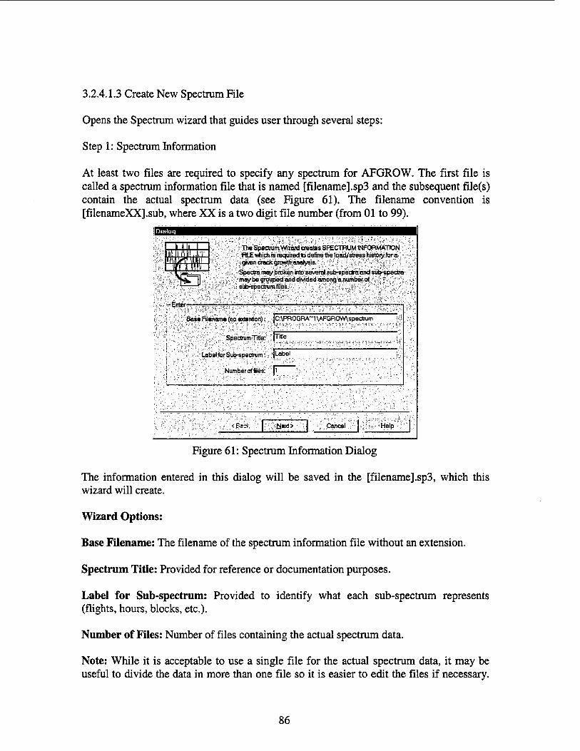
3.2.4.1.3 Create New Spectrum File
Opens the Spectrum wizard that guides user through several steps:
Step 1: Spectrum Information
At least two files are required to specify any spectrum for AFGROW. The first file is called a spectrum information file that is named [filename].sp3 and the subsequent file(s) contain the actual spectrum data (see Figure 61). The filename convention is [filenameXX].sub, where XX is a two digit file number (from 01 to 99).
rafWBi
T>e*SpecwnxW^createsSreCTOUMl^QBW«rT10N: RLEwhichis requiredto definethetoad/sti . given crack growth analysts
Spectra may Isiib-spedra •maybe groUpadand^ividedemdngaTOmbefpf.«^ If,"'";, stib^spi
-Enter'TT—.•^,?.„-^.^..:.;..—.:.'.';..
., ? Base Filename (no extention):
:-' 'i ' SpectrumTrtle'
■ Label for Sub-spectrum:
Number of files:
|G\PROGRA~1 \AFGROW\spectrum
"(Title
>\lobe\ ;^
I1.
<Back, ^üexo. Cancel ;.Help
Figure 61: Spectrum Information Dialog
The information entered in this dialog will be saved in the [filename].sp3, which this wizard will create.
Wizard Options:
Base Filename: The filename of the spectrum information file without an extension.
Spectrum Title: Provided for reference or documentation purposes.
Label for Sub-spectrum: Provided to identify what each sub-spectrum represents (flights, hours, blocks, etc.).
Number of Files: Number of files containing the actual spectrum data.
Note: While it is acceptable to use a single file for the actual spectrum data, it may be useful to divide the data in more than one file so it is easier to edit the files if necessary.
86

AFGROW can work with a spectrum file of any size, but no sub-spectrum may exceed 4MB. The number of sub-spectra is unlimited.
Help: Displays the help topic for this step. Users may also press Fl for help.
Cancel: Cancels your previous actions and closes the Wizard.
Back: Disabled in this step.
Next: Move forward to the next step.
Step 2: Type of Spectrum Type of spectrum
A cycle by cycle spectrum is one in which each maxmin - ' .. load/stress is applied tor one (1) cycle This may be thought of
as a real time spectrum The blocked spectrum is one where each mox-min pair is applied*» some finite number of cycles
Many tames, spectra are presented m this format to save . computer time and space.
-In many cases, the use of the blocked format produces very little difference in terms of the Äanalysis; In general; the more times a spectrum is: repeated, the less the differences using
blocked or cyde-by-cyde spectra
«SeleäType:ö?jSj^Är<*|
ff jBlocked Cydesj
, <~ CyctebyCyde
-<£ack : )$&&£ iCance!? IBelp,f
Figure 62: Spectrum Type Dialog
AFGROW uses the term Blocked spectrum, to indicate that each Max, Min Stress level may consist of multiple cycles.
The term Cycle by Cycle means that each Max, Min Stress level may only have one cycle.
Note: Although AFGROW expects a Cycle by Cycle spectrum to have one cycle per level, the format of the data must be in the form Max Min 1, where 1 is the number of cycles. In this way, the file format is consistent. AFGROW will not except a Cycle x Cycle spectrum unless the number of cycles for each stress level is one.
87

Wizard Options:
Help: Displays the help topic for this step. Users may also press Fl for help.
Cancel: Cancels your previous actions and closes the Wizard.
Back: Move back to the previous step.
Next: Move forward to the next step.
Step 3: Number of Sub-Spectra Number of Sub-spectra
?There ere Nmittin manual mode. placeaorilhB numberpf. sub-spedrathet can makeup aspeetrum.The limits are10 sub-spectra per file
Enter Number of Sub-spectra in file #1 -
^'*lumbef]of.SuWpe^'r;y;>'|l
'Import from file)
»:=F ■;Biawse.v!
<Eack täext>: Cancel' Help
Figure 63: Sub-Spectra Dialog
Wizard Options:
Number of Sub-spectra: used only for manual spectrum data entry.
Import from File: The wizard can import a complete spectrum file containing an unlimited number of sub-spectra. This file may be a standard AFGROW spectrum file *.sub or a user created ASCII file in the following format:
[number of sub-spectra]
[number of stress levels in a given sub-spectrum]
[max stress] [min stress] [cycles]
[number of stress levels in a given sub-spectrum]
88
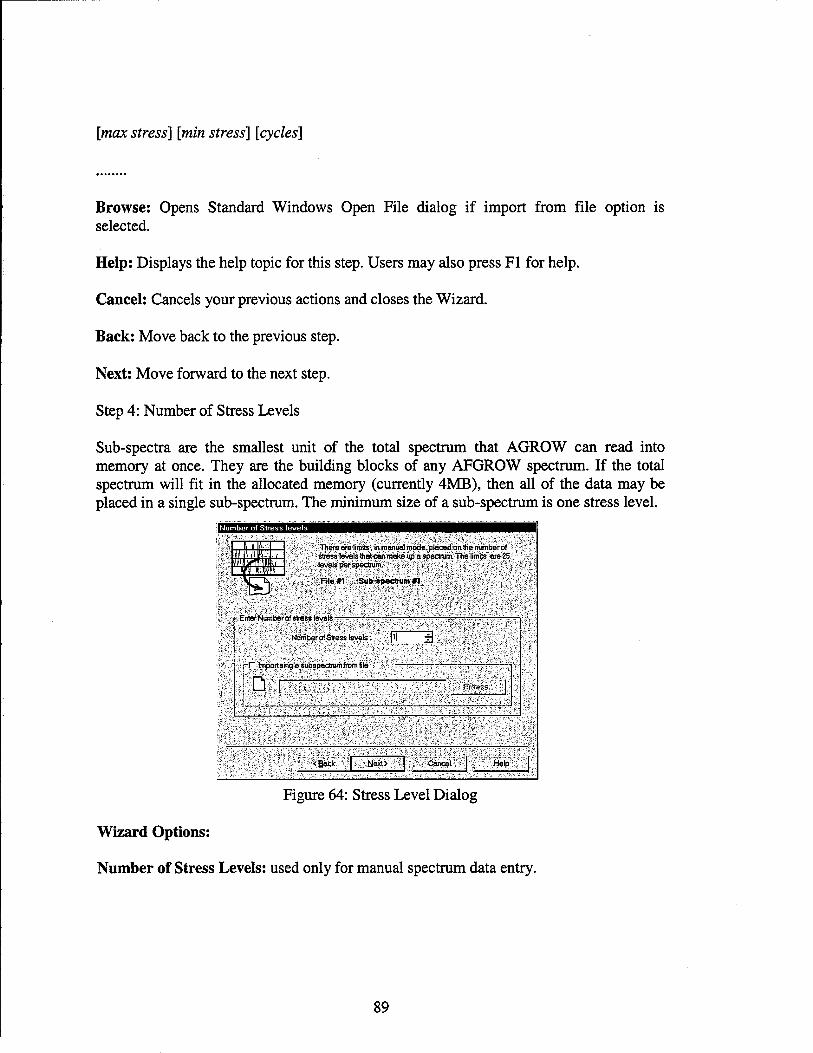
[max stress] [min stress] [cycles]
Browse: Opens Standard Windows Open File dialog if import from file option is selected.
Help: Displays the help topic for this step. Users may also press Fl for help.
Cancel: Cancels your previous actions and closes the Wizard.
Back: Move back to the previous step.
Next: Move forward to the next step.
Step 4: Number of Stress Levels
Sub-spectra are the smallest unit of the total spectrum that AGROW can read into memory at once. They are the building blocks of any AFGROW spectrum. If the total spectrum will fit in the allocated memory (currently 4MB), then all of the data may be placed in a single sub-spectrum. The minimum size of a sub-spectrum is one stress level.
Number of Stress evels
*'' ?1ihöire: ere lirp^Vtncniohäo! ,^ode^laradonl^e-humber'of -^ ^stress levels that con moke up a spedram;<The limits are 25 levels per spectrum. r - ' '
File#1 ^Sub-spectrum #1
- Enter Number of stress levels -— ——
/ Number of Stress levels: , jl
-: * .'f ■ I~ import single subspBctrumftorti i\e :f "< £; *
SSÄSfäKS'»'? ±1
■ Srovrae 1 ! Ü | ■ .
'i'".'-?5!';":ä--?'S:-'r;'
■■«Back tjext> I Cancel Help"
Figure 64: Stress Level Dialog
Wizard Options:
Number of Stress Levels: used only for manual spectrum data entry.
89

Import single sub-spectrum from file: The wizard can import a file containing the stress levels for a given sub-spectrum. This file must be an ASCII file in the following format:
[number of stress levels in a given sub-spectrum]
[max stress] [min stress] [cycles]
[max stress] [min stress] [cycles]
[max stress] [min stress] [cycles]
Browse: Opens Standard Windows Open File dialog if import from file option is selected.
Help: Displays the help topic for this step. Users may also press Fl for help.
Cancel: Cancels your previous actions and closes the Wizard.
Back: Move back to the previous step.
Next: Move forward to the next step.
Step 5: Stress Levels
This page is only used for manual spectrum data entry. Maximum of 25 stress levels may be entered manually. If larger spectra are required, use the read sub-spectrum from file option.
File#1 Sub-spectrum #1 ä'-.:V;'r
'-' • Input Spectrum Stress /Load levels inform Büon in the ifollowmgferrhat' ; \-" c;
r Enter Stress Levels.^
^rT :S* Min Cycles
1 1.000000 0.000000 1 2 0.700000 -0.300000 10 3 0.800000 0.100000 50
«flock :| .•ijea> | ■■: Cancel | Help
Figure 65: Stress Levels
90
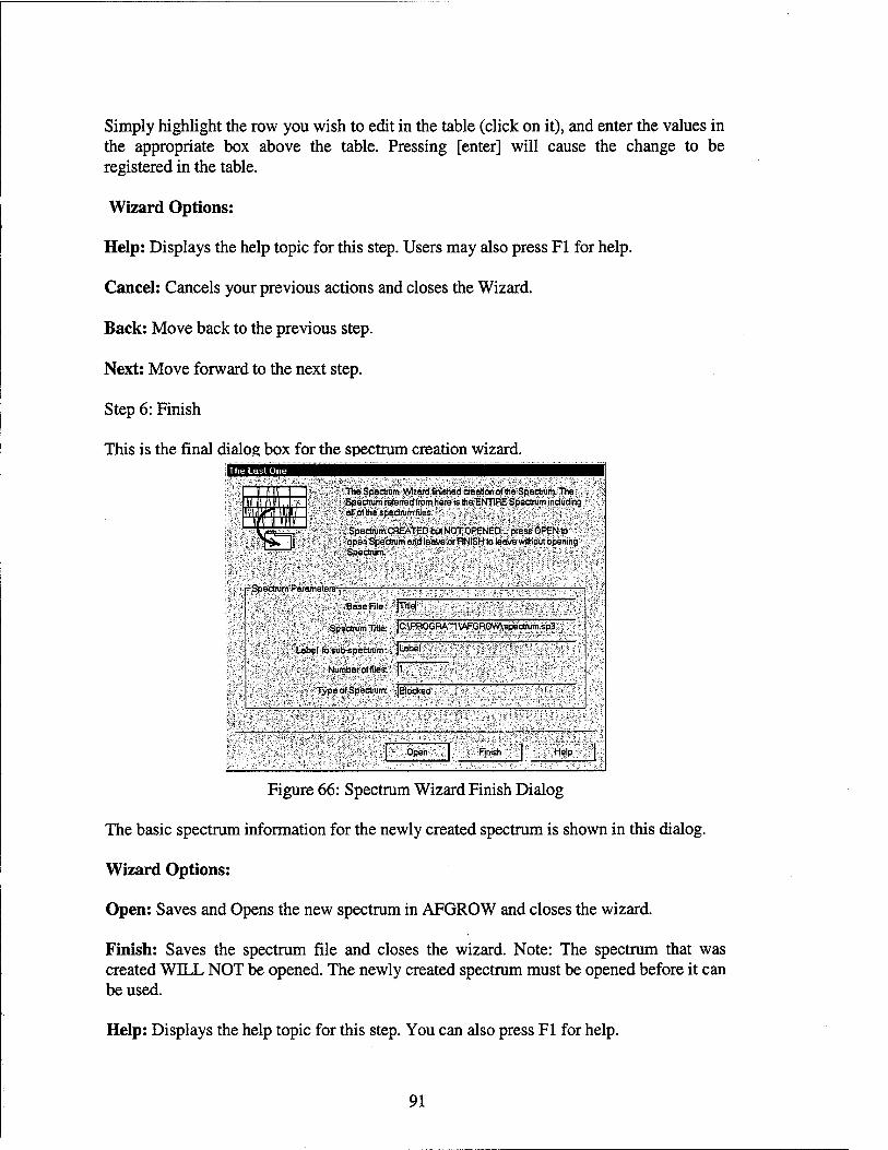
Simply highlight the row you wish to edit in the table (click on it), and enter the values in the appropriate box above the table. Pressing [enter] will cause the change to be registered in the table.
Wizard Options:
Help: Displays the help topic for this step. Users may also press Fl for help.
Cancel: Cancels your previous actions and closes the Wizard.
Back: Move back to the previous step.
Next: Move forward to the next step.
Step 6: Finish
This is the final dialog box for the spectrum creation wizard. The Last One
"iTheSpectrum-'WizardSnishedoeolion^fthe Spectrum.The , Spsdrumrefetied from here is the ENTIRE Spectrum including
^ all ofthe spectrum files.
Spectrum CREATED but NOT OPENED.. press OPEN to ;äDpenSpeöramand:le»»orB^^ .Spectrum. ~ • .'"-
tSfleer™m;Pärametersf
- Base File: jTrtlel
> Spectrum Title: |O.\PR0GRA~1\AFGR0W\spectrum sp3
Label fo sub-spectrum: |Label ~ < „•',,'
,' Number offfles: l> , •TypeofSpeetrum: (Blocked:
Bppeh Finish Help
Figure 66: Spectrum Wizard Finish Dialog
The basic spectrum information for the newly created spectrum is shown in this dialog.
Wizard Options:
Open: Saves and Opens the new spectrum in AFGROW and closes the wizard.
Finish: Saves the spectrum file and closes the wizard. Note: The spectrum that was created WELL NOT be opened. The newly created spectrum must be opened before it can be used.
Help: Displays the help topic for this step. You can also press Fl for help.
91
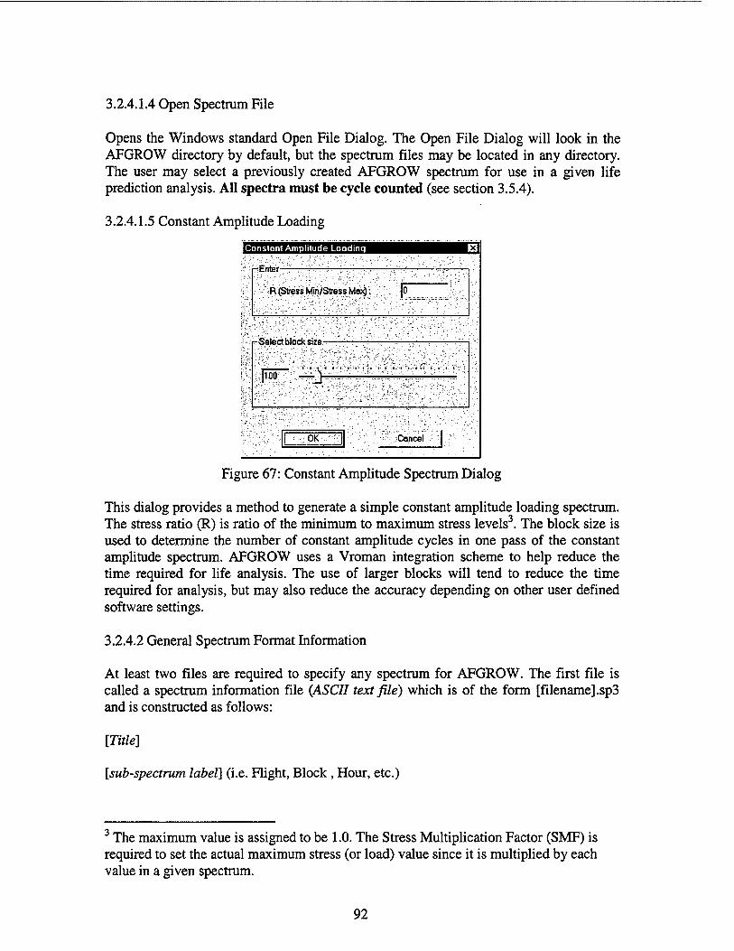
3.2.4.1.4 Open Spectrum File
Opens the Windows standard Open File Dialog. The Open File Dialog will look in the AFGROW directory by default, but the spectrum files may be located in any directory. The user may select a previously created AFGROW spectrum for use in a given life prediction analysis. All spectra must be cycle counted (see section 3.5.4).
3.2.4.1.5 Constant Amplitude Loading
Constant Amplitude Loading
pEnte'r-
R (Stress Min/Stress Ma^:
-Select block size -
100 -£
OK ,: Cancel
Figure 67: Constant Amplitude Spectrum Dialog
This dialog provides a method to generate a simple constant amplitude loading spectrum. The stress ratio (R) is ratio of the minimum to maximum stress levels3. The block size is used to determine the number of constant amplitude cycles in one pass of the constant amplitude spectrum. AFGROW uses a Vroman integration scheme to help reduce the time required for life analysis. The use of larger blocks will tend to reduce the time required for analysis, but may also reduce the accuracy depending on other user defined software settings.
3.2.4.2 General Spectrum Format Information
At least two files are required to specify any spectrum for AFGROW. The first file is called a spectrum information file (ASCII text file) which is of the form [filename].sp3 and is constructed as follows:
[Title]
[sub-spectrum label] (i.e. Flight, Block , Hour, etc.)
3 The maximum value is assigned to be 1.0. The Stress Multiplication Factor (SMF) is required to set the actual maximum stress (or load) value since it is multiplied by each value in a given spectrum.
92
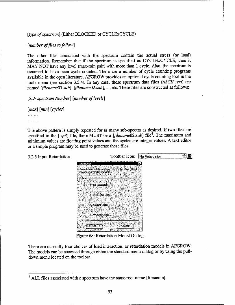
[type of spectrum] (Either BLOCKED or CYCLExCYCLE)
[number of files to follow]
The other files associated with the spectrum contain the actual stress (or load) information. Remember that if the spectrum is specified as CYCLExCYCLE, then it MAY NOT have any level (max-min pair) with more than 1 cycle. Also, the spectrum is assumed to have been cycle counted. There are a number of cycle counting programs available in the open literature. AFGROW provides an optional cycle counting tool in the tools menu (see section 3.5.4). In any case, these spectrum data files (ASCII text) are named [filenameOLsub], [filename02.sub],..., etc. These files are constructed as follows:
[Sub-spectrum Number] [number of levels]
[max] [min] [cycles]
The above pattern is simply repeated for as many sub-spectra as desired. If two files are specified in the [.sp3] file, there MUST be a [filename02.sub] file4. The maximum and minimum values are floating point values and the cycles are integer values. A text editor or a simple program may be used to generate these files.
3.2.5 Input Retardation Toolbar Icon: |j^Reteidatigii
IftetardoSon modelsusedio eccourrtforthe effected load ; sequence of crack growth rate.' " <■ _x'„ \ .- I
pSeledS
P Ha Retardation
C MlenborgModel.
•ifÜos ura Model: ;jv
:r MeelerModel...-:
L .g-J iiGäsncelK
Figure 68: Retardation Model Dialog
There are currently four choices of load interaction, or retardation models in AFGROW. The models can be accessed through either the standard menu dialog or by using the pull- down menu located on the toolbar.
ATI, files associated with a spectrum have the same root name [filename].
93

Note: Each model has a user adjustable parameter that is used to tune the model to fit actual test data. Ideally, a parameter should be a material constant, which is independent of other variables such as spectrum sequence or load level. Some models seem to work better than others in this regard, but there is a need to reproduce results for various types of retardation models. These models are provided to be used at the users discretion and responsibility.
The details of the No Retardation, Generalized Willenborg, Closure, and Wheeler models are given in the following sections.
3.2.5.1 No Retardation
This is the default option in AFGROW. When this option is selected, no spectrum load interaction effects will be assumed.
3.2.5.2 Generalized Willenborg Model
The Generalized Willenborg model [43] is one of the most common load interaction models used in crack growth life prediction programs. The model is based on early fracture mechanics work performed at Wright-Patterson AFB, OH and was named after a student who worked on the model. The model uses an "effective" stress intensity factor based on the size of the yield zone in front of the crack tip. The formulation of the Willenborg retardation model used in AFGROW is given below:
Kmax(eff) = Kmax - Kred
Kmin(eff) = Kmin - Kred
R(eff) = Kmin(eff)/Kmax(eff)
Kred=0 Kmax(ol) 1_(* xW'-Kmzx V Ry(oD
<t> = (1 - AKphreshoid/KmaxyCSOR -1)
Ry(ol) = (Kmax(ol)\
Yield '{ 1 )
^ PSXn}
Where:
x: Crack Length
x(ol): Crack Length at Overload
94

AKihreshow • Threshold value of DK at R = 0
Yield: Material yield strength
PSX : Stress State in a Given Crack Growth Direction (2.0 (Plane Stress) - 6.0 (Plane Strain))
The subscript (ol) refers to an overload condition. It is changed each time that an applied maximum stress (or load) exceeds a previous maximum, or when the current yield zone size (Ry) grows beyond the yield zone created by an overload (Ry(ol)). The value, 0, is simply a parameter used in the Generalized Willenborg model. The AK-rhreshow is the lowest value of AK that will cause a crack to grow for R = 0. The value is based on user input for the crack growth rate model being used in a given prediction.
Retardation Parameter:
Willenborq Retardation Parameters
/T\ The Willenborg model uses on 'effective1 stress äj^JjJ intensity factor based on the size of yield zone in
front of the cracktipto-accountfortheeffectof load sequence on crack growth rate.
sEnterS
Shutoff Overload Ratio (SOLR): 12.5
SOK-? Cancel
Figure 69: Willenborg Retardation Parameter Dialog
SOR : Shut-off Ratio - Ratio of overload maximum stress to the subsequent maximum stress required to arrest crack growth
The exact value of the SOR is varied to adjust the life prediction to match test results. Ideally, the SOR should be a material parameter, which is insensitive to spectrum or stress level. However, this does not always work out. The following is a list of common SOR values for some materials:
Aluminum: SOR = 3.0
Titanium: SOR = 2.7
Steel: SOR = 2.0
Many crack growth programs use the Chang acceleration model [44] with the Willenborg retardation model to account for the effect of compressive stress (or load) cycles. The Chang model requires the use of negative stress intensity values. AFGROW does not consider negative stress intensity factors to be valid (in general). In place of the Chang
95

acceleration model, AFGROW uses the following method to account for the effect of compressive stresses (or loads):
( Ry(ol) =
(, 1-0.9 ABS compression
overload
Yl
/;
Ry(ol)
Using the absolute value of the ratio of the compressive stress (or load) to the overload stress (or load) reduces the size of the current overload yield zone. This method will NOT increase the effective stress intensity; it will merely reduce the retarding effect of a previous overload. Therefore, the Willenborg model used in AFGROW can NEVER result in a life prediction that is less than the life prediction with no retardation.
3.2.5.3 Closure Model Closure Retardation Parameters
m The Closure mode) uses an -single parameter (CfO) to determine the opening level as the crack gro*4hto accounttar
"the effeaofload sequence on crack grovrih rale. CfO is the ratio of the stress opening level to the maximum stress at R-0.
Enter Opening Load Ratio @ R-0,0 -
;; fOLR @ R-oiO: JÖ1
.OK
Cancel
1 ij~-Afgrow uses an thrtioJ Crack Opening Load Ratio to begin -analysis using the Closure model.
rSelectr
ff Determine initial OLRfrom first level in spectrum
C. Manually input initial OLR
Figure 70: Closure Retardation Model Dialog
The closure model in AFGROW is a fairly simple single-parameter plasticity model. The model is based on early fracture mechanics work by Erdogan and Elber and more recent models proposed by Dr. Matthew Creager and Dr Sunder [2-4]. The model, developed by Mr. James Harter, basically expanded a constant closure model originally developed by Dr. Creager while he and Mr. Harter were involved in performing damage tolerance analyses for the B-2 Bomber in 1982-83.
It is important to understand that this model is called a closure model because it is based on the idea that the crack is "closed" when no load is applied and a certain load must be applied to "open" the crack tip. Some researchers believe that yielded material in the wake of a growing crack acts as a wedge behind the crack tip [45]. This yielded material is forced to be in compression by the elastic material surrounding it. Other researchers believe that this plastic wake is merely a surface phenomenon caused by the difference between the plane stress state at the surface and an internal plane strain state. They believe that the apparent contact behind the crack tip is merely the result of natural stress
96
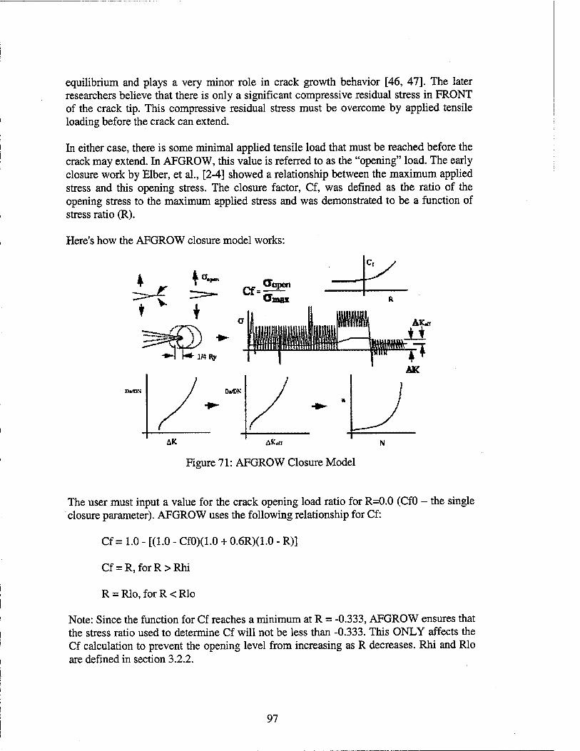
equilibrium and plays a very minor role in crack growth behavior [46, 47]. The later researchers believe that there is only a significant compressive residual stress in FRONT of the crack tip. This compressive residual stress must be overcome by applied tensile loading before the crack can extend.
In either case, there is some minimal applied tensile load that must be reached before the crack may extend. In AFGROW, this value is referred to as the "opening" load. The early closure work by Eiber, et al., [2-4] showed a relationship between the maximum applied stress and this opening stress. The closure factor, Cf, was defined as the ratio of the opening stress to the maximum applied stress and was demonstrated to be a function of stress ratio (R).
Here's how the AFGROW closure model works:
H|Mtt
lttfy
Da/DK
AK AK*» N
Figure 71: AFGROW Closure Model
The user must input a value for the crack opening load ratio for R=0.0 (CfO - the single closure parameter). AFGROW uses the following relationship for Cf:
Cf = 1.0 - [(1.0 - Cf0)(1.0 + 0.6R)(1.0 - R)]
Cf = R,forR>Rhi
R = Rlo,forR<Rlo
Note: Since the function for Cf reaches a minimum at R = -0.333, AFGROW ensures that the stress ratio used to determine Cf will not be less than -0.333. This ONLY affects the Cf calculation to prevent the opening level from increasing as R decreases. Rhi and Rio are defined in section 3.2.2.
97

The initial crack opening level can either be determined from the first cycle of the input spectrum OR may be input by the user in case any previous load history is known.
According to work by Dr. Sunder, the Cf value expected for a given stress ratio will not be reached until the crack grows 1/4 of the way through the yield zone created by the maximum stress. The opening level is varied linearly from the current value within the 1/4 yield zone distance. AFGROW keeps track of the current overload cycle by defining an overload condition whenever (crack length + yield zone) > previous overload - as is the case in the Willenborg model.
Compressive loads/stresses are treated a bit differently in that the opening level may be INSTANTANEOUSLY shifted to the level determined by the equation above for an R value equal to the ratio of the compressive minimum load/stress to the current maximum overload load/stress. The INSTANT change in opening level is made IF the maximum value for a given cycle IS an overload (yield zone extends beyond previous overload case) AND the opening level is LOWER than the current opening level OR the maximum value for a given cycle IS NOT an overload AND the opening level (based on the R value determined from the compressive value and the current overload) is LOWER than the current opening level. The idea is that while a crack must grow into the plastic wake of tensile overloads to fully develop a given opening level, a compressive cycle can instantly cause the residual stress field to be changed. If any given compressive load/stress is not low enough to cause the opening level to fall below the current value, then there is no reason to change the opening stress.
When an overload cycle contains a compressive minimum, the overload yield zone size is reduced by 10 percent of the absolute value of the stress ratio for that cycle. This reduction is made to help account for the effect of the compressive minimum. This reduces the effect of the overload since it will take fewer subsequent cycles to grow through a smaller overload yield zone. The quantity, 10 percent, was determined based on actual test data for common aircraft alloys tested in-house at Wright-Patterson AFB and some very helpful data provided by Mr. Kevin Walker [48].
Finally, an effective AK is determined from the difference between the maximum K and the K value for the opening load/stress level. Since the input crack growth rate data is NOT based on the effective AK, a conversion back to apparent AK is made in the crack growth rate module. This conversion, however, is based on the Cf value for the current load cycle.
Sparen, = ^ej? ^^ ^R> 0.0
AKapparent=^^yJorR<0.05
This relationship is used here because AFGROW uses K^, not AK, when R < 0.0
98
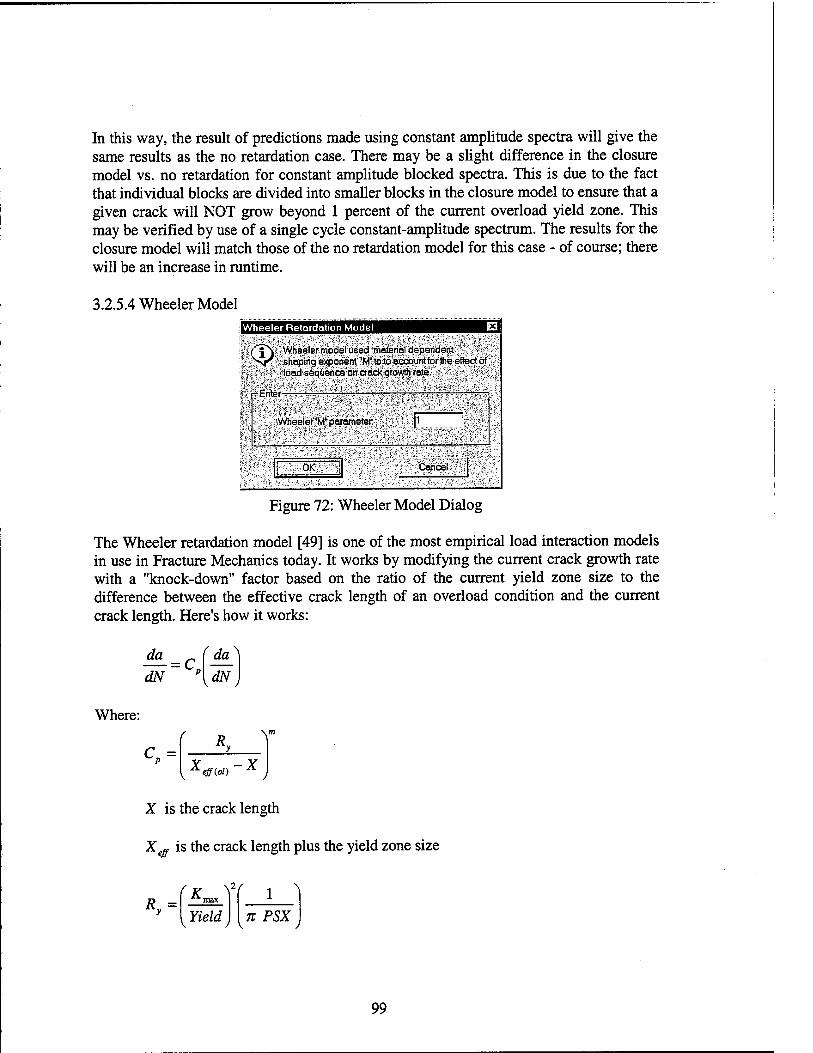
In this way, the result of predictions made using constant amplitude spectra will give the same results as the no retardation case. There may be a slight difference in the closure model vs. no retardation for constant amplitude blocked spectra. This is due to the fact that individual blocks are divided into smaller blocks in the closure model to ensure that a given crack will NOT grow beyond 1 percent of the current overload yield zone. This may be verified by use of a single cycle constant-amplitude spectrum. The results for the closure model will match those of the no retardation model for this case - of course; there will be an increase in runtime.
3.2.5.4 Wheeler Model Wheeler Retardation Model
("j^N Wheeler model used material dependent i'fssjT shaping exponent 'M' to to accountfor the effect of
load sequence on crack growth rate.
rSEnteW
.j^/^eler^fcejaraeter,.
mm Cancel
Figure 72: Wheeler Model Dialog
The Wheeler retardation model [49] is one of the most empirical load interaction models in use in Fracture Mechanics today. It works by modifying the current crack growth rate with a "knock-down" factor based on the ratio of the current yield zone size to the difference between the effective crack length of an overload condition and the current crack length. Here's how it works:
da _c
dN " [dN)
Where:
CP = R„
Xeff(.ol) X
X is the crack length
X ~ is the crack length plus the yield zone size
Ry =
(K V max
Yield /
I 1 ^ n PSX \ )
99

Note: AFGROW uses the Irwin yield zone equation (and the current stress state) to determine the yield zone size. The subscript (ol) refers to an overload condition. It is changed each time that an applied maximum stress (or load) exceeds a previous maximum, or when the current yield zone size (Ry) grows beyond the yield zone created by an overload (Ry(ol)). PSX is the stress state for the given crack length (2 - Plane Stress, 6 - Plane Strain).
Retardation Parameter:
m: Wheeler exponent
The value of the Wheeler exponent, m, is determined from test data for a given material, spectrum, stress level, etc. As mentioned above, this model is extremely empirical and the m value, which gives good correlation to test data, has been known to be dependent on MANY test parameters. Users should use this model with caution.
3.2.6 Input Stress State Toolbar Icon:
8 Stress State EJl
<$> The Stress State Date provide & means of approximating the actual value of
'_;'yield zone sizeand fracture toughness in each crack grovyth direction.
; <? Determine Stress State automatically
f Enter Stress State manually
{-■v^-QK--;:^
Cancel
Figure 73: Stress State Dialog
There are currently two choices in AFGROW for Stress State: Automatic Stress State Determination and User Specified. AFGROW uses a stress state index of real numbers that range from 2 to 6. The range was chosen because of the relationship between stress state and the Irwin yield zone size.
Plane Stress: Yield Zone Size -(Kn V 1
[ Yield j In
Plane Strain: Yield Zone Size = ( Yield j
V 1 6n
AFGROW uses the stress state index to determine the yield zone size, which is required for the load interation models, AND to determine the appropriate value of fracture toughness. The yield zone size is determined as follows:
100

c Yield Zone Size = max
Yield {j.ndex)n
The actual value of fracture toughness that defines the stress intensity failure limit for a given geometry is often called the apparent fracture toughness since it is determined by the given geometry and applied failure stress. The highest possible value of fracture toughness is the plane stress fracture toughness and the lowest possible value is the plane strain fracture toughness. The plane stress and strain fracture toughness values are material properties. The apparent fracture toughness value is determined by a linear interpolation between the plane strain (KIC) and plane stress (Kc) fracture toughness values input by the user.
Apparent Fracture Toughness = Klc + -^ (Kc - KJC)
The stress state index is a function of the specimen thickness and maximum applied stress intensity. Specimens that are relatively thin are generally operate under plane stress conditions (index = 2.0) and thick specimens are generally plane strain (index = 6.0).
3.2.6.1 Automatic Stress State Determination
The default choice for stress state determination in AFGROW is to automatically determine the stress state index based on KmaX and specimen thickness for each applied load/stress cycle. The relationship between K^, thickness (t), and stress state index [50] is:
Index =6.7037- 1.4972 flT ^2
max
Yield t
If Index > 6.0, Index = 6.0 (Plane Strain)
If Index < 2.0, Index = 2.0 (Plane Stress)
The above relationship has been verified with fracture test data for several metal alloys. The complete details will be published at a later date. The test results are shown in Figure 74.
101

Stress State Information
a 5
«5
« 707S-T651 Aluminum
A THAI-4VAMS 431*3 Annealed
■ 4340-135 KsISleel
—AFGROV Model
(Kcrit/Yield)7t
Figure 74: Stress State Information
According to David Broek [51], the plane strain condition is:
Plane Strain (index = 6.0): .( Kc
(Yield <0A7t
The ASTM standard for a plane strain condition [52] is:
t>2.5 ( K . *
Yield
The ASTM standard is slightly more conservative, but it meets Dr Broek's plane strain condition.
There is no definitive reference for the plane stress condition. The test data shown in Figure 74 for three common aircraft alloys (aluminum, titanium, and steel) led Mr. Harter [50] to believe that the following plane stress condition may be applied for these alloys:
Plane Stress (index=2.0): ( K . }
Yield >nt
A linear equation was used to determine intermediate stress state indices for conditions between the plane stress and strain limits. Plane stress and strain fracture toughness values were known for the alloys used in the test program. Each center cracked (MT) specimen was pre-cracked to various crack lengths and loaded monotonically to failure. The failure stress and crack length was used to determine the critical stress intensity
102

factor. The stress state index was determined by linear interpolation based on the plane stress and strain fracture toughness values for each material.
3.2.6.2 User Specified Stress State
Users have an option to input stress state index values. If this option is selected, AFGROW will use a constant value for stress state index in a given crack growth dimension. The index range is a real number from 2 to 6, where 2 is used for Plane Stress and 6 for Plane Strain. The user-specified value(s) will remain constant during the life prediction calculations and will be used to determine the apparent fracture toughness.
3.2.7 Input User-Defined Beta Toolbar Icon:
Users can input their own solutions through the user-defined beta option. However, to use this option, the user must first select either the 1-D or 2-D user defined geometry from the Standard Solutions dialog (see section 3.2.3). Beta factors are defined as follows:
ß = —== ; Where x is the appropriate crack length oJitx
The crack length dimension in the thickness direction is the a-dimension and the crack length in the width direction is the c-dimension. Application and user defined solutions are identified in the beta solution column in the geometry tab of the model dialog (see Figure 47, Section 3.2.3). There are only two user-defined models among the standard solutions since AFGROW only handles 1-D or 2-D cracks. These geometries are simply generic models, which depict either a 2-D crack (2 crack dimensions) or a 1-D crack (1 crack dimension). Since the user inputs the beta values, the actual geometry is taken into account by the beta values themselves. The image in the animation frame is merely showing a generic view since it is difficult to show all possible user-defined geometries.
3.2.7.1 One-Dimensional User Defined Betas
The one-dimensional user-defined beta option is used when a user has an existing stress intensity factor solution (in the form of a beta table) for any crack that may be described with one length dimension (1-D) to input in AFGROW.
The geometric beta values are NOT calculated by AFGROW, but are merely interpolated from a one-dimensional user defined table of beta values. Users must supply beta values at various crack lengths so that the appropriate value at a given crack length may be interpolated. This model is shown as an edge cracked plate in the animation frame. The representation of the model is merely meant to indicate the one-dimensional nature of the crack. It was not possible to create representations of all possible geometries that may be modeled using user defined beta factors.
103

For the [c] crack length dimension: K = aJncß(c)
When the user-defined beta option is selected for a through crack case, the dialog box shown in Figure 75 appears:
User-Input Beta Table(Throuqh-Cruck)
m Enter creek length and Betafectore.BWcuirentmoc|elgeoRielry»8l000(user* .defined perMhrough cradej. this table is wed afterthe transition to a through-crack.
Beta factors tor any crack length are obtained by ÜneorinterpolatotrornthistobleiFof crack lengths outside the range of ihe table, the nearestvelue jn the table will be used.
-Enter up to 25 sets —. '■rv': : "■':.■'■■■ '
, Number of "C Sets: s il Set .'■ C | Beta . -1 r- 0.1
0.2 0.3 0.5 2 1 ''vS
2 . :3 ': .«.■.:■
-5 ■.'■■:
pFileT-——
Span j
. si : ; Save |
Help
Figure 75: Through Crack User-Defined Beta Table Dialog
The initial crack length should be the same as the initial part through crack length in the C direction, which will become the through crack. This is because it may be difficult to know what that dimension will be by the time the crack transitions and it is important that the input data cover the entire range of possibilities. AFGROW will NOT extrapolate user-defined betas and will simply use the nearest data in the event the data are out of range.
If the user-defined through crack input data are saved, AFGROW will give it a .bet extension which will be visible the next time this dialog is opened (clicking on the read button will open it again). Just remember which directory the data are in if you decide to save to some directory other than the default.
3.2.7.2 Two-Dimensional User Defined Betas E This option is used when a user has an existing stress intensity factor solution (in the form of a beta table) for any crack which may be described with two length dimensions (2-D) to input in AFGROW.
The geometric beta values are NOT calculated by AFGROW, but are merely interpolated from a two-dimensional user defined table of beta values. Users must supply beta values at various crack lengths so that the appropriate value at a given crack length may be interpolated. This model is shown as a corner cracked plate in the animation frame. The representation of the model is merely meant to indicate the two dimensional nature of the crack. It was not possible to create representations of all possible geometries that may be modeled using user defined beta factors.
104

For the [a] crack length dimension: K = a^jnaß(a)
For the [c] crack length dimension: K = a^Jncßic)
When the beta icon (or User-Defined Beta menu option) is selected, the dialog shown in Figure 76 will appear:
i ;\^;,Forpart*roaghfl8ws/OM ■: " specif useHnputbetetedors , ,
'"' BBft ";~^6 ^our P°,rrt 'n1erPolaiion requires es input betafadorvaluesloMreterence -"■'HlfiSa luring - -
propagation. ', -
apj*. y ^I'l^ie JineorjintetpolatibrT method reqü^Wmotnces'#a^^ ,.. ..... "¥;beta*actQrsin,iheWand'Cdtre^ :>
covesalltradcshapesposstbledunngpropagotton^ , ' Tlia accuracy of this meftpdv^
■ ;ttr>Bar icterpcrfaSondote-meyortyb«rea^ \ : must be antaredmanual^ v ^
^ff^oWpoW interpofatjorj' \
;; C bnearmterpolation -:-"<hi
<Qeak ) flaxt> '|;; VHelp-
Figure 76: 2-D User Input Beta Dialog
Since beta values for a 2-D crack are dependent on crack shape (a/c), a matrix of beta values are required to determine the appropriate stress intensity factors for each dimension (assuming the dimensions are independent). The two dimensions of crack growth are allowed to grow based on the stress intensity for each dimension. It is not possible to anticipate the changes in crack shape that are possible as the 2-D crack grows under any arbitrary loading.
There are currently two choices in AFGROW to input User Defined Betas for Part- Through Cracks: Four Point and Linear. Actually both use linear interpolation. The Four Point method attempts to provide a simpler method of interpolation, which is based on Schijve's weighted interpolation [53] (without weights, which are model specific). The Linear method is a straightforward double table look-up that must be read from a file.
3.2.7.2.1 Four-Point User-Defined Beta Values
AFGROW will produce the following dialog with crack length suggestions (which may be changed as desired - within the guidelines noted) if the four-point method is selected (see Figure 77).
105
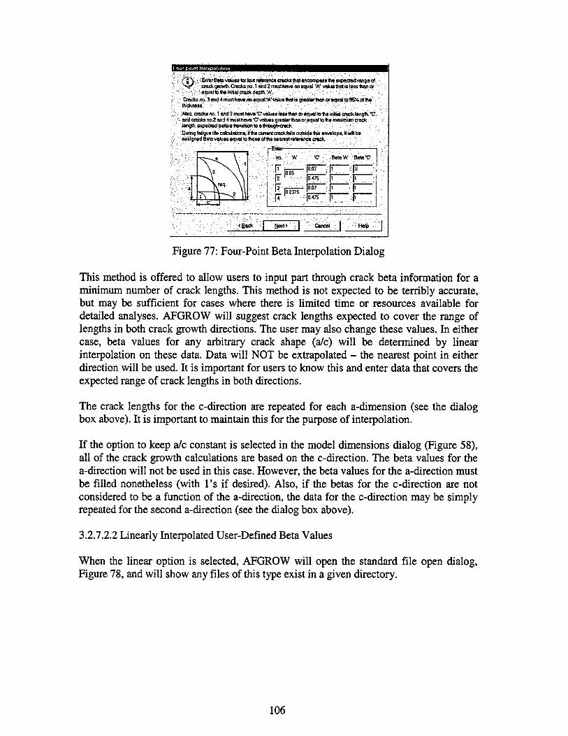
IJ.IIII.I.IUILÜJI.I.II.
m ■Enter Bete values for tour reference crack» ttiatoncomposs the expected range of, •crodtg^o^; Cracks no. 1 and2masthoveanequol W valuethatis less than or:
;':equdtoftekiitidcrockdflpth.W. . ;• /'"" ; CmcksnQ.3önd^mu$thüveanequal'A'vaJu8tiaiagfeataflhonorequa]to95Ho<the
'■.-thickness""'. *■■■■ , ' >;■..' '.'■'■■,.''■' " '.■':'■ '.'■" Also, cracks no.1* end 3 must have 'O values less then or eqüeJ to fteinWelc>ack length, t?.
> end cra^rra.2 and 4 must he\*'C\ralues greater . length, expected before fransKian to a through-crack. i
.During fatigue life r^culotiorK/rf : - assigned Beta values equal to ftose of the nearest reference crack.
1> 1 --•N2 1! . c .
^no. • 'A'
, jr p........ ;:■[?':-■:■
L. |0 2375
-■"■'■'G': , - Beta 'A' 'Beta-C
|0.07 >:H ■ \0A7S 1' }
, JQ.07
••JMTT" 1'
"I' |i
■1
;.<fiack tjexl> | Cancal Help
Figure 77: Four-Point Beta Interpolation Dialog
This method is offered to allow users to input part through crack beta information for a minimum number of crack lengths. This method is not expected to be terribly accurate, but may be sufficient for cases where there is limited time or resources available for detailed analyses. AFGROW will suggest crack lengths expected to cover the range of lengths in both crack growth directions. The user may also change these values. In either case, beta values for any arbitrary crack shape (a/c) will be determined by linear interpolation on these data. Data will NOT be extrapolated - the nearest point in either direction will be used. It is important for users to know this and enter data that covers the expected range of crack lengths in both directions.
The crack lengths for the c-direction are repeated for each a-dimension (see the dialog box above). It is important to maintain this for the purpose of interpolation.
If the option to keep a/c constant is selected in the model dimensions dialog (Figure 58), all of the crack growth calculations are based on the c-direction. The beta values for the a-direction will not be used in this case. However, the beta values for the a-direction must be filled nonetheless (with l's if desired). Also, if the betas for the c-direction are not considered to be a function of the a-direction, the data for the c-direction may be simply repeated for the second a-direction (see the dialog box above).
3.2.7.2.2 Linearly Interpolated User-Defined Beta Values
When the linear option is selected, AFGROW will open the standard file open dialog, Figure 78, and will show any files of this type exist in a given directory.
106
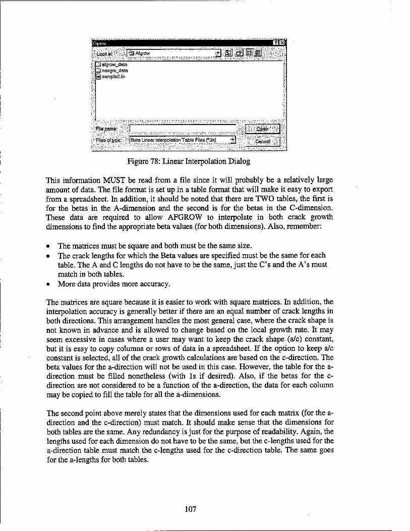
:ilStä>pfeinS €3 Afgrow "3 M äilWi 3) afgrow_data S3 nasgro_data |5] sample2.lin
,Rle nattier. stSpen;*
?Hlesof^pe: • :; (Beta Linear Interpolation Table Files C"\lin) 1 ^Cancel
Figure 78: Linear Interpolation Dialog
This information MUST be read from a file since it will probably be a relatively large amount of data. The file format is set up in a table format that will make it easy to export from a spreadsheet. In addition, it should be noted that there are TWO tables, the first is for the betas in the A-dimension and the second is for the betas in the C-dimension. These data are required to allow AFGROW to interpolate in both crack growth dimensions to find the appropriate beta values (for both dimensions). Also, remember:
• The matrices must be square and both must be the same size. • The crack lengths for which the Beta values are specified must be the same for each
table. The A and C lengths do not have to be the same, just the C's and the A's must match in both tables.
• More data provides more accuracy.
The matrices are square because it is easier to work with square matrices. In addition, the interpolation accuracy is generally better if there are an equal number of crack lengths in both directions. This arrangement handles the most general case, where the crack shape is not known in advance and is allowed to change based on the local growth rate. It may seem excessive in cases where a user may want to keep the crack shape (a/c) constant, but it is easy to copy columns or rows of data in a spreadsheet. If the option to keep a/c constant is selected, all of the crack growth calculations are based on the c-direction. The beta values for the a-direction will not be used in this case. However, the table for the a- direction must be filled nonetheless (with Is if desired). Also, if the betas for the c- direction are not considered to be a function of the a-direction, the data for each column may be copied to fill the table for all the a-dimensions.
The second point above merely states that the dimensions used for each matrix (for the a- direction and the c-direction) must match. It should make sense that the dimensions for both tables are the same. Any redundancy is just for the purpose of readability. Again, the lengths used for each dimension do not have to be the same, but the c-lengths used for the a-direction table must match the c-lengths used for the c-direction table. The same goes for the a-lengths for both tables.
107
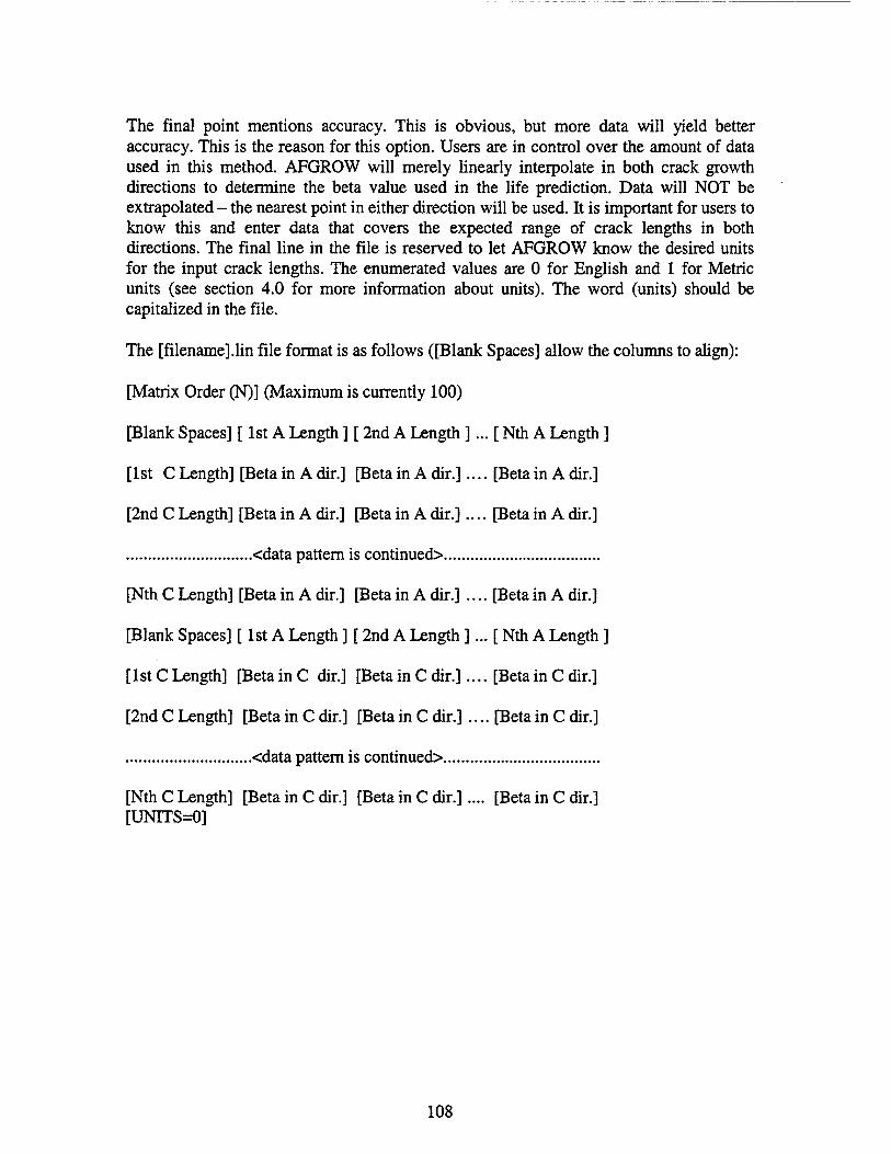
The final point mentions accuracy. This is obvious, but more data will yield better accuracy. This is the reason for this option. Users are in control over the amount of data used in this method. AFGROW will merely linearly interpolate in both crack growth directions to determine the beta value used in the life prediction. Data will NOT be extrapolated - the nearest point in either direction will be used. It is important for users to know this and enter data that covers the expected range of crack lengths in both directions. The final line in the file is reserved to let AFGROW know the desired units for the input crack lengths. The enumerated values are 0 for English and 1 for Metric units (see section 4.0 for more information about units). The word (units) should be capitalized in the file.
The [filename].lin file format is as follows ([Blank Spaces] allow the columns to align):
[Matrix Order (N)] (Maximum is currently 100)
[Blank Spaces] [ 1st A Length ] [ 2nd A Length ]... [ Nth A Length ]
[1st C Length] [Beta in A dir.] [Beta in A dir.].... [Beta in A dir.]
[2nd C Length] [Beta in A dir.] [Beta in A dir.].... [Beta in A dir.]
<data pattern is continued>
[Nth C Length] [Beta in A dir.] [Beta in A dir.] .... [Beta in A dir.]
[Blank Spaces] [ 1st A Length ] [ 2nd A Length ]... [ Nth A Length ]
[1st C Length] [Betain C dir.] [Betain C dir.].... [Betain C dir.]
[2nd C Length] [Beta in C dir.] [Beta in C dir.] .... [Beta in C dir.]
<data pattern is continued^»
[Nth C Length] [Beta in C dir.] [Beta in C dir.].... [Beta in C dir.] [UNTTS=0]
108

3.2.8 Input Environment Toolbar Icon:
Currently, AFGROW allows cyclic environmental effects to be determined based on crack growth rate data obtained for the environment of interest. In the case of some environmental effects (i.e. corrosion (material loss)), the effect may be merely limited to local increased stress levels. However, some environmental effects can have a direct effect on the crack growth rate behavior of a given material. In the later case, the cyclic environmental effect model may be used to more accurately predict crack growth life. AFGROW allows as many as six separate applications of the same or different environments as indicated in Figure 79.
[Environment E3
i|§| Direction 'C j Direction W J s^"
ill v ' ~0K"
Hie | Start I End Cancel • C:\Program Files\AFGR... ! 0.15 ] 0.25 |
• C:\Program Files\AFGR... i 0.5 ! 0.75 i; Add
Remove
Edit
Figure 79: Environment Dialog
For the example above, the depiction of the applied environments is indicated on the model as shown in Figure 80.
Figure 80: Environmental Depiction in the Animation Frame
Each application of a given environment is shown (color-coded) on the specimen in the animation frame. For now, the environmental capability is only available when the "Harter T-Method" (section 3.2.2.4) for crack growth rate data representation is used. The reason for this is because separate crack growth rate data files must be created for the environmental data. The tabular data format was considered to be the most accurate means of representing actual crack growth rate data. The initial capability was designed prior to the development of the tabular look-up crack growth rate model (section 3.2.2.5). The material title used for each material in the material data file in the "Harter T-Method" is compared to the title lines in the environment data file to ensure that data for the same material are being used.
109
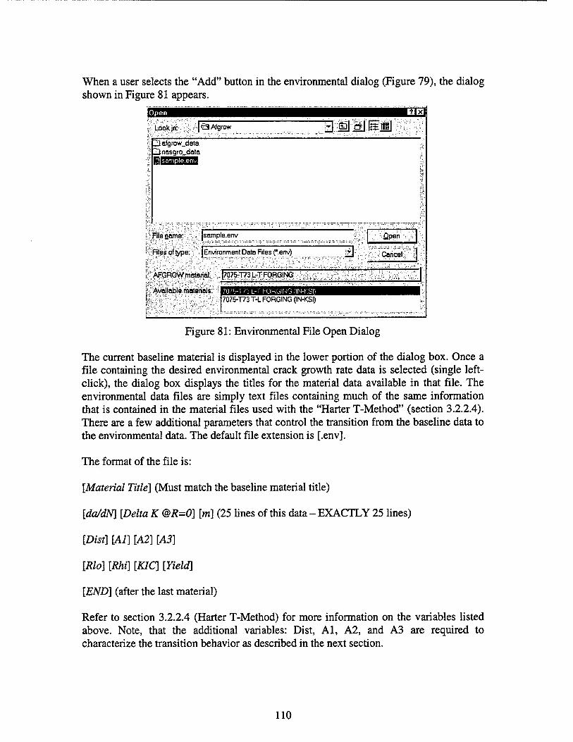
When a user selects the "Add" button in the environmental dialog (Figure 79), the dialog shown in Figure 81 appears.
7 Look in: a Afgrow
j3ofgrow_data 23nasgro_data PH5BJHHE
Filename: '.. jsample.env
, Rlescrfjype; "'. [Environment Data Files f.env)
\ßpeh
~E Cancel;
AFGROW material. -|70?5-T73bT FORGING,
Available materials:
Figure 81: Environmental File Open Dialog
The current baseline material is displayed in the lower portion of the dialog box. Once a file containing the desired environmental crack growth rate data is selected (single left- click), the dialog box displays the titles for the material data available in that file. The environmental data files are simply text files containing much of the same information that is contained in the material files used with the "Harter T-Method" (section 3.2.2.4). There are a few additional parameters that control the transition from the baseline data to the environmental data. The default file extension is [.env].
The format of the file is:
[Material Title] (Must match the baseline material title)
[da/dN] [Delta K @R=0] [m] (25 lines of this data - EXACTLY 25 lines)
[Dist] [Al] [A2] [A3]
[Rio] [Rhi] [KIC] [Yield]
[END] (after the last material)
Refer to section 3.2.2.4 (Harter T-Method) for more information on the variables listed above. Note, that the additional variables: Dist, Al, A2, and A3 are required to characterize the transition behavior as described in the next section.
110
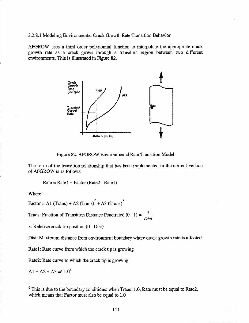
3.2.8.1 Modeling Environmental Crack Growth Rate Transition Behavior
AFGROW uses a third order polynomial function to interpolate the appropriate crack growth rate as a crack grows through a transition region between two different environments. This is illustrated in Figure 82.
Crack Growtfi Rate fän/Cyde)
Tratudert Growth Rate
AiR
»
Delta K (in. Jcsi; *
Figure 82: AFGROW Environmental Rate Transition Model
The form of the transition relationship that has been implemented in the current version of AFGROW is as follows:
Rate = Ratel + Factor (Rate2 - Ratel)
Where:
Factor = Al (Trans) + A2 (Trans) + A3 (Trans)
JC Trans: Fraction of Transition Distance Penetrated (0 -1) = —
Dist
x: Relative crack tip position (0 - Dist)
Dist: Maximum distance from environment boundary where crack growth rate is affected
Ratel: Rate curve from which the crack tip is growing
Rate2: Rate curve to which the crack tip is growing
Al+A2 + A3=! 1.06
6 This is due to the boundary conditions: when Trans=1.0, Rate must be equal to Rate2, which means that Factor must also be equal to 1.0
111

3.2.9 Input Beta Correction
AFGROW includes an ability to estimate stress intensity factors for cases, which may not be an EXACT match for one of the stress intensity solutions in the AFGROW library (section 3.2.3). For example, a case is being modeled with a high stress gradient. It is unlikely that an exact solution would be available, and the creation of a boundary or finite element model would be time consuming. AFGROW offers a method to approximate the solution using a beta correction technique (see Figure 83).
Beta Correction Factors
//"j\ ^AFGROW allows the stress intensfyfactorsolutioris tobe modified Nvf', by using multiplication (Beta Correction)factors. -
othe;stressatthe;
crack origin. TTdistanra^from thecerterpolrt of ft JSeterttypegfjDaW ■ ;<,-:.&,.—'\ l...^:'_:n '•'.; ;.'—..'',.; :.~.;~
■;£• Normalized Stress '"■ ■ OBeta Correction Factors
^ Enter stress and V. Use up to 25 sets——
Number of Sets:, :>%m- Set":--'-;- >"rV':'--';'r Sfr.0) V: SM- •ftr ■■';,'. :}:'Q'-:^ 1
: r 0.001 0.01 0.1 0.5
0.9 1| oss " 1 0.B 1
0.79 1
■■•■•':2':;:■-''
::~"3 ",;■■:■
.'■-.A ■■;?:.
V-.S'N'V 1 0.785 1 ::■;■ :::J'T;V>'*
JOK-
Cancel
r File-
Save
Open
Figure 83: Beta Correction Factor Dialog
Users have the option of entering normalized stress values in the crack plane and allow AFGROW to calculate beta correction factors or enter pre-determined beta correction values.
3.2.9.1 Determine Beta Correction Factors Using Normalized Stresses
AFGROW employs a Gaussian integration method, which uses a point load stress intensity solution from the Tada, Paris, and Irwin Stress Intensity Handbook [54] to integrate a given 2-D unflawed stress field (in the crack plane) to estimate stress intensity values at user defined crack length increments.
Users should choose the standard model with a stress field that is as close as possible to the stress field of interest. Then determine the ratio of the unflawed stress field of interest to the unflawed stress field for the chosen geometry at various crack length intervals. A maximum of 25 points may be input to describe the stress distribution. The intervals should be selected such that linear interpolation would provide a reasonable curve fit
112
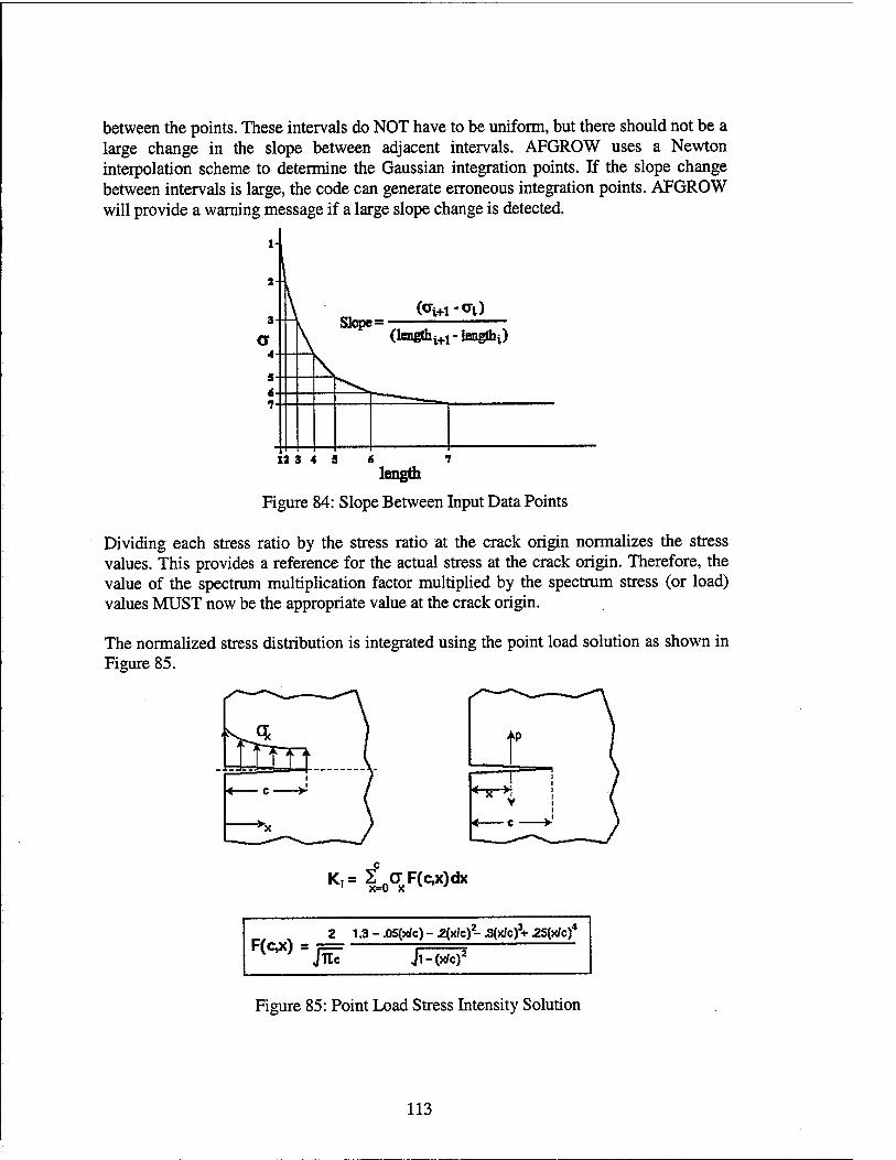
between the points. These intervals do NOT have to be uniform, but there should not be a large change in the slope between adjacent intervals. AFGROW uses a Newton interpolation scheme to determine the Gaussian integration points. If the slope change between intervals is large, the code can generate erroneous integration points. AFGROW will provide a warning message if a large slope change is detected.
1-
S--
3- - \ „ (<*Vfl -CO
\
MVgK (kngthi+1-lengrhi)
6- •}-■
12 3 4 S 6 7 length
Figure 84: Slope Between Input Data Points
Dividing each stress ratio by the stress ratio at the crack origin normalizes the stress values. This provides a reference for the actual stress at the crack origin. Therefore, the value of the spectrum multiplication factor multiplied by the spectrum stress (or load) values MUST now be the appropriate value at the crack origin.
The normalized stress distribution is integrated using the point load solution as shown in Figure 85.
K,= 2=0CTF(cx)dx
Figure 85: Point Load Stress Intensity Solution
113

The beta correction factor is calculated by dividing the stress intensity determined by integrating the input stress field by the stress intensity value for a unit stress distribution at each crack length increment. Obviously, this method is not exact since it can't account for stress field changes as the crack grows, but it is fairly good - especially at shorter crack lengths where most of the life is spent.
AFGROW multiplies the resulting beta correction factor by the beta factor for the user- selected model at a given crack length. These corrected beta values are printed in the output list in AFGROW in the beta column.
For the [a] crack length dimension: Ka = a^jna ßa
For the [c] crack length dimension: K* = c^Jjrcßc
Where, in this case: ß = ßmodei * ßconection
In two-dimensional cases, users must refer to the x and y dimensions in the animation frame and the dimensions shown in the beta correction dialog (see Figure 83). The length dimension, r, shown in the dialog box is the radial distance from the crack origin. The input stress ratio values are shown for (r,0) - along the y = 0 axis and (0,r) - along the x = Oaxis.
There are a few important points to remember:
• The stress field is normalized to the stress at the crack origin • The value of the maximum spectrum stress MUST correspond to the stress at the
crack origin • Choose crack length intervals such that linear interpolation on stress ratio is adequate
between points • When entering stress ratio data for 1-D, values of 1.0 should be input for the other
dimensions • If there is a stress gradient in only 1-D, enter values of 1.0 for all points in the other
dimensions • Accuracy increases with the number of points
3.2.9.2 Enter Beta Correction Factors Manually
Users have the option to enter beta correction factors directly instead of allowing AFGROW to calculate them. There may be cases where a user simply wants to apply beta correction factors that have been obtained from some external source. To enter beta correction factors manually, simply select "Beta Correction Factors" in the "Select Type of Data" section of the beta correction dialog box (see Figure 83).
The beta correction at the crack origin is set equal to 1.0 by default only because the values are required to be normalized at the crack origin when stress values are input. The
114

beta correction value at the crack origin can only be used as an interpolation limit since all cracks must have a finite length. The first user supplied beta value should be entered for a crack length less than the initial crack size for interpolation purposes. In two- dimensional cases, users must refer to the x and y dimensions in the animation frame and the dimensions shown in the beta correction dialog (see Figure 83). The length dimension, r, shown in the dialog box is the radial distance from the crack origin. The input stress ratio values are shown for (r, 0) along the y = 0 axis (for the width direction) and (0, r) along the x = 0 axis (for the thickness direction). AFGROW will NOT extrapolate beta correction values for crack lengths extending past the input table limits.
3.2.10 Input Residual Stresses
AFGROW can account for the existence of residual stresses by calculating additive residual stress intensities at user defined crack length increments. The dialog shown in Figure 86 will appear when the residual stress option is selected.
Residua Stresses
V: sicracfcgrowth by reading inatoble-otresidualstressesiosÄlunctionof.» ;?trarj<1encjlh,thartAFGROW uses these ^
'Residual Stress IntensityFactors' (SIF)
S(x,y) - value of a stress in Z axis direction: .r--distance from the center point of the crack along*: or Y- axis;
iSeted^eotüatef C Stress ><~-Residual K;
r Enter stressend Y. Use up to 25 sets-
Numberof Sets: ]6 ^'jrj . -
.SetV'j :;:r5iK'3 [;S(M))'s' kwrn^ i ~®-pig" 0 -2.4 -2.4
£Z-''A" 0.02 0.04
-1.2 o
: "2.4 : '■^■-■■Sii ; -2.4 ^i'-"'-'-\ 0.25 0.55 -2.4 ■<£y.
';-£-:.»'S: 0.5 : 0.5 0 Ä ■KSiMK 1 0.45 0 tl
;Geherete SlgtaJoleiising '-j
& Gauss Integration
f Weight Function'
SOKS I^lpencei'
Figure 86: Residual Stress Dialog
Normally, AFGROW does not consider negative values of stress intensity (K) since K is not defined for compression. However, in this application, negative stress intensities can be used since the residual Ks are merely added to the stress intensities caused by the applied loads.
When you use this option, AFGROW will print out the residual K value each time it prints out the standard crack growth information. It is important that you input stress information for the entire range of crack growth since AFGROW WILL NOT extrapolate and will just use the last or nearest applicable value.
115
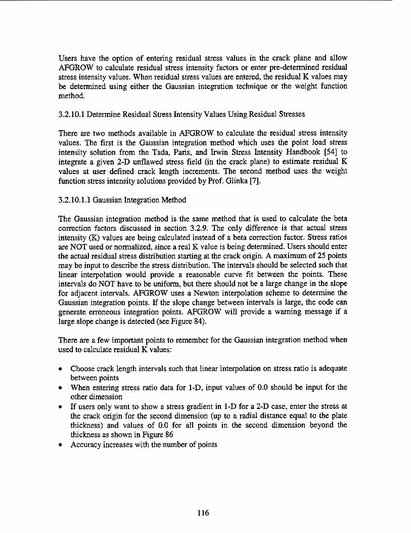
Users have the option of entering residual stress values in the crack plane and allow AFGROW to calculate residual stress intensity factors or enter pre-determined residual stress intensity values. When residual stress values are entered, the residual K values may be determined using either the Gaussian integration technique or the weight function method.
3.2.10.1 Determine Residual Stress Intensity Values Using Residual Stresses
There are two methods available in AFGROW to calculate the residual stress intensity values. The first is the Gaussian integration method which uses the point load stress intensity solution from the Tada, Paris, and Irwin Stress Intensity Handbook [54] to integrate a given 2-D unflawed stress field (in the crack plane) to estimate residual K values at user defined crack length increments. The second method uses the weight function stress intensity solutions provided by Prof. Glinka [7].
3.2.10.1.1 Gaussian Integration Method
The Gaussian integration method is the same method that is used to calculate the beta correction factors discussed in section 3.2.9. The only difference is that actual stress intensity (K) values are being calculated instead of a beta correction factor. Stress ratios are NOT used or normalized, since a real K value is being determined. Users should enter the actual residual stress distribution starting at the crack origin. A maximum of 25 points may be input to describe the stress distribution. The intervals should be selected such that linear interpolation would provide a reasonable curve fit between the points. These intervals do NOT have to be uniform, but there should not be a large change in the slope for adjacent intervals. AFGROW uses a Newton interpolation scheme to determine the Gaussian integration points. If the slope change between intervals is large, the code can generate erroneous integration points. AFGROW will provide a warning message if a large slope change is detected (see Figure 84).
There are a few important points to remember for the Gaussian integration method when used to calculate residual K values:
• Choose crack length intervals such that linear interpolation on stress ratio is adequate between points
• When entering stress ratio data for 1-D, input values of 0.0 should be input for the other dimension
• If users only want to show a stress gradient in 1-D for a 2-D case, enter the stress at the crack origin for the second dimension (up to a radial distance equal to the plate thickness) and values of 0.0 for all points in the second dimension beyond the thickness as shown in Figure 86
• Accuracy increases with the number of points
116
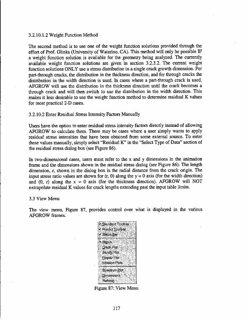
3.2.10.1.2 Weight Function Method
The second method is to use one of the weight function solutions provided through the effort of Prof. Glinka (University of Waterloo, CA). This method will only be possible IF a weight function solution is available for the geometry being analyzed. The currently available weight function solutions are given in section 3.2.3.2. The current weight function solutions ONLY use a stress distribution in a single crack growth dimension. For part-through cracks, the distribution in the thickness direction, and for through cracks the distribution in the width direction is used. In cases where a part-through crack is used, AFGROW will use the distribution in the thickness direction until the crack becomes a through crack and will then switch to use the distribution in the width direction. This makes it less desirable to use the weight function method to determine residual K values for most practical 2-D cases.
3.2.10.2 Enter Residual Stress Intensity Factors Manually
Users have the option to enter residual stress intensity factors directly instead of allowing AFGROW to calculate them. There may be cases where a user simply wants to apply residual stress intensities that have been obtained from some external source. To enter these values manually, simply select "Residual K" in the "Select Type of Data" section of the residual stress dialog box (see Figure 86).
In two-dimensional cases, users must refer to the x and y dimensions in the animation frame and the dimensions shown in the residual stress dialog (see Figure 86). The length dimension, r, shown in the dialog box is the radial distance from the crack origin. The input stress ratio values are shown for (r, 0) along the y = 0 axis (for the width direction) and (0, r) along the x = 0 axis (for the thickness direction). AFGROW will NOT extrapolate residual K values for crack lengths extending past the input table limits.
3.3 View Menu
The view menu, Figure 87, provides control over what is displayed in the various AFGROW frames.
* Standard Toolbar •* Predict Toolbar v Status Bar
• Status \ Crack Plot : da/dNHot
ßepair Plot' Initiation Plots
Spectrum Plot
Dimensions Refresh
Figure 87: View Menu
117

The view menu is divided into three sections. The upper section controls the display of the toolbar and status bar. The middle section controls the display of the main frame. The bottom section controls additional special features displayed in the animation frame.
3.3.1 View Standard Toolbar
The standard toolbar, Figure 88, allows a user to perform many common Microsoft Windows® operations:
Figure 88: Standard Toolbar
When selected, the standard toolbar appears in the AFGROW window, and a checkmark appears by this item in the view menu. This toolbar is dockable and can be relocated at the top, sides, or bottom of the AFGROW window. It may also be placed as a floating toolbar anywhere on the desktop. The toolbar is moved by placing the mouse pointer in a blank area between two icons, holding down the left mouse button, and dragging the toolbar to the desired location.
The function of each icon is displayed through the standard Windows help when you move the mouse over the icon.
3.3.2 View Predict Toolbar
The predict toolbar, Figure 89, allows a user to use shortcuts to perform many common operations required to perform crack growth life predictions:
!► ► ■ Hm 'BBM-hP. No Retardation £] E IB\*
Figure 89: Predict Toolbar
When selected, the predict toolbar appears in the AFGROW window, and a checkmark appears by this item in the view menu. This toolbar is dockable and can be relocated at the top, sides, or bottom of the AFGROW window. It may also be placed as a floating toolbar anywhere on the desktop. The toolbar is moved by placing the mouse pointer in a blank area between two icons, holding down the left mouse button, and dragging the toolbar to the desired location.
The function of each icon is displayed through the standard Windows help when you move the mouse over the icon.
3.3.3 View Status Bar
The status toolbar is found in the margin at the bottom of the output frame (see Figure 20).
118

The purpose of the status toolbar is to provide additional information related to a given analysis. The status bar is a tool that Microsoft provides and should not be confused with the "status view" which is used by AFGROW to display the current input data in the upper left window. For more details, refer to section 2.6.
3.3.4 View Status
The status window is one of the optional "windows" which may be displayed in the upper left-hand window (main frame) in the AFGROW main window (see Figure 9).
The window may be displayed by clicking on the view, status menu buttons on the main AFGROW menu OR by simply using the pull-down menu in the upper left-hand AFGROW window. For more details, refer to section 2.1.1.
3.3.5 View Crack Plot
The crack length plotting capability allows a user to graphically examine the crack growth life predictions being performed by AFGROW in real time (see Figure 11). When selected, a new menu item (Plots) will appear in the menu bar. This menu item provides access to the same features given in the rebar tool in the main frame. For more details, refer to section 2.1.2.
3.3.6 View da/dN Plot
The da/dN plotting capability allows a user to graphically examine the crack growth rate properties to be used by AFGROW (see Figure 13). When selected, a new menu item (da/dN Plots) will appear in the menu bar. This menu item provides access to the same features given in the rebar tool in the main frame. For more details, refer to section 2.1.3.
3.3.7 View Repair Plot
The repair plotting capability allows a user to graphically examine the beta correction plots for up to eight repair designs (see Figure 14). For more details, refer to section 2.1.4.
3.3.8 View Initiation Plots
The initiation plotting capability allows a user to graphically examine the cyclic stress- strain and strain-life plots for the current input data (see Figure 15). When selected, a new menu item (Initiation Plots) will appear in the menu bar. This menu item provides access to the same features given in the rebar tool in the main frame. For more details, refer to section 2.1.5.
119

3.3.9 View Spectram Plot
The da/dN plotting capability allows a user to graphically examine the spectrum being used by AFGROW (see Figure 90).
X AFGROW- [CAProqrom Files\AFGROW\d1staf sp31 |;E'Bl8 Input ,View Predig: ^ndow Help -Jfiixj [ 3jglBj_ ^Nfel^l Iff l^l]|^l^«l MBiliil^l^l FTiiSde^ 3ti'Mir ■IBM III UMJIUIBUI
npfpn in »in mnfi|^|i>iiwmifi|ip
•0.2667
'ForHelp. press Fl
1798 3596 5394 7193 8991 10769 12588 14386 16184 17983
(^English T
Figure 90: Spectrum Plot
When this option is selected, a new spectrum window will be created. While in this view, several tools in the toolbar are now grayed out since they serve no purpose in the spectrum view window. The color of the data plotted is changed for each sub-spectrum.
Users can zoom-in the spectrum view by using the mouse and dragging out the area to view on the spectrum plot. The entire spectrum is always displayed in the upper area of this view. Users can also adjust the view in the upper area of the window by using the mouse and dragging the highlighted box.
3.3.10 View Dimensions
The Dimensions option in the View menu simply shows the definition of the basic geometric dimensions for the current model being analyzed. For example, the corner cracked hole dimensions are shown in Figure 91.
V w
1 >■ *-e_
Figure 91: Specimen Dimensions
120
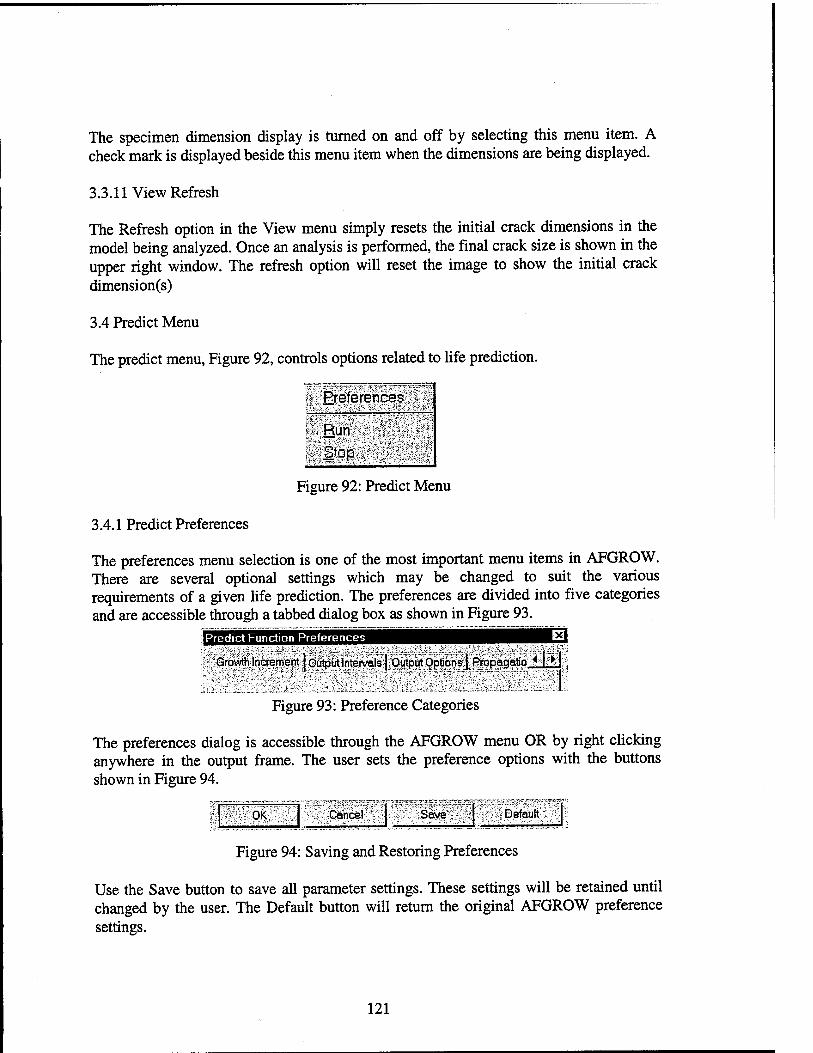
The specimen dimension display is turned on and off by selecting this menu item. A check mark is displayed beside this menu item when the dimensions are being displayed.
3.3.11 View Refresh
The Refresh option in the View menu simply resets the initial crack dimensions in the model being analyzed. Once an analysis is performed, the final crack size is shown in the upper right window. The refresh option will reset the image to show the initial crack dimension(s)
3.4 Predict Menu
The predict menu, Figure 92, controls options related to life prediction.
Preferences
ßun Stop
Figure 92: Predict Menu
3.4.1 Predict Preferences
The preferences menu selection is one of the most important menu items in AFGROW. There are several optional settings which may be changed to suit the various requirements of a given life prediction. The preferences are divided into five categories and are accessible through a tabbed dialog box as shown in Figure 93.
Predict Function Preferences
mm Growth Increment Output Intervals | Output Options | Propagatio
Figure 93: Preference Categories
The preferences dialog is accessible through the AFGROW menu OR by right clicking anywhere in the output frame. The user sets the preference options with the buttons shown in Figure 94.
80K2 Cancel 'iSimi Default
Figure 94: Saving and Restoring Preferences
Use the Save button to save all parameter settings. These settings will be retained until changed by the user. The Default button will return the original AFGROW preference settings.
121
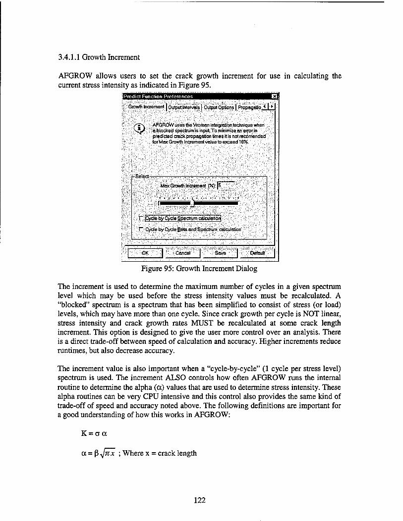
3.4.1.1 Growth Increment
AFGROW allows users to set the crack growth increment for use in calculating the current stress intensity as indicated in Figure 95.
Predict Function Preferences
Growth increment | QutpKerVals | Output Options | Probiaaotio < I >
M ; AFGROW uses the Vromon integrotibn technique when ' d blocked spectrurrüs inputTo minimize an error in ■.'■ predicted crack propagation times it is not recomended for Max Growth Increment value to exceed 10%.
feSelectW-
Mex Growth-Increment (%):;-|5;
; l~ jCycle rjyC^ )'."%
I" Cycle by Cycle Betel and Spectrum, calculation
OK: • Cancel SaveT : Default
Figure 95: Growth Increment Dialog
The increment is used to determine the maximum number of cycles in a given spectrum level which may be used before the stress intensity values must be recalculated. A "blocked" spectrum is a spectrum that has been simplified to consist of stress (or load) levels, which may have more than one cycle. Since crack growth per cycle is NOT linear, stress intensity and crack growth rates MUST be recalculated at some crack length increment. This option is designed to give the user more control over an analysis. There is a direct trade-off between speed of calculation and accuracy. Higher increments reduce runtimes, but also decrease accuracy.
The increment value is also important when a "cycle-by-cycle" (1 cycle per stress level) spectrum is used. The increment ALSO controls how often AFGROW runs the internal routine to determine the alpha (a) values that are used to determine stress intensity. These alpha routines can be very CPU intensive and this control also provides the same kind of trade-off of speed and accuracy noted above. The following definitions are important for a good understanding of how this works in AFGROW:
K=fJOC
a = ß TJTZX ; Where x = crack length
122
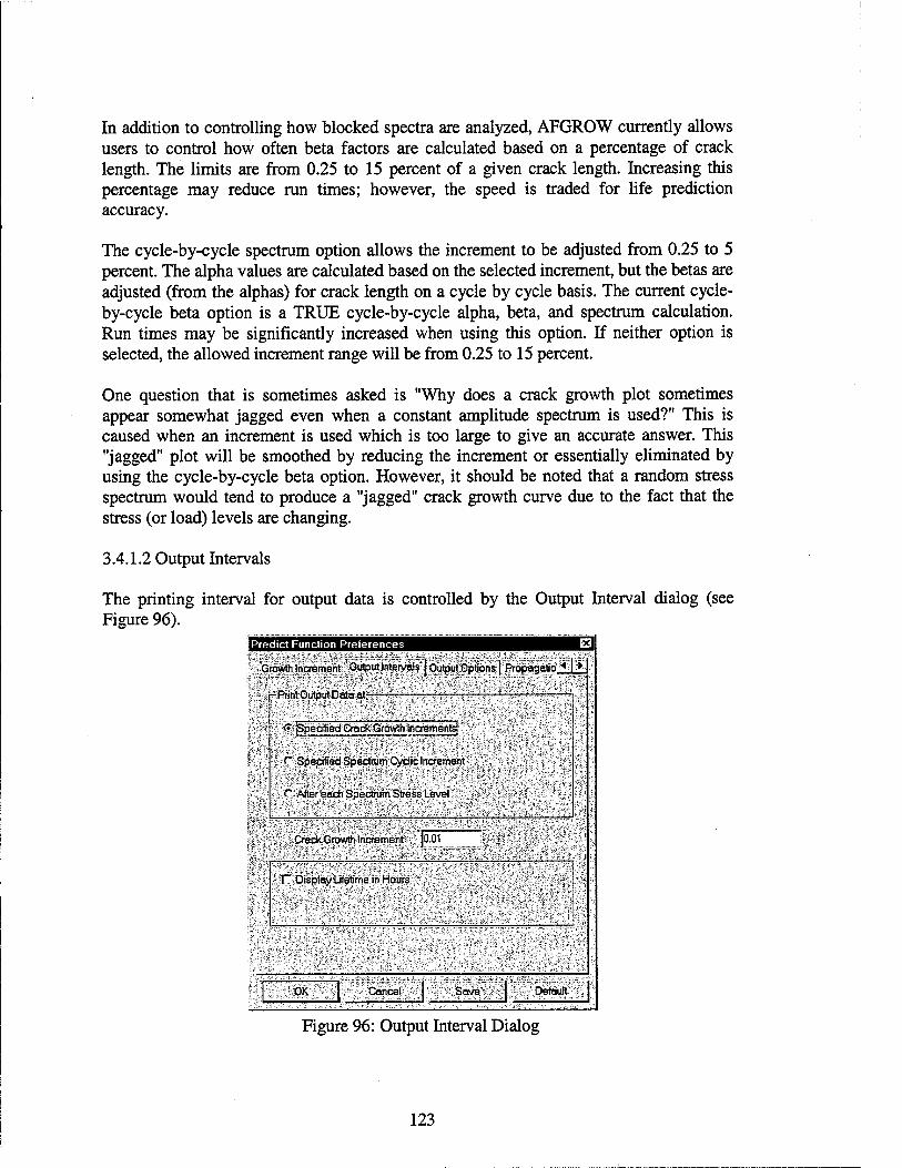
In addition to controlling how blocked spectra are analyzed, AFGROW currently allows users to control how often beta factors are calculated based on a percentage of crack length. The limits are from 0.25 to 15 percent of a given crack length. Increasing this percentage may reduce run times; however, the speed is traded for life prediction accuracy.
The cycle-by-cycle spectrum option allows the increment to be adjusted from 0.25 to 5 percent. The alpha values are calculated based on the selected increment, but the betas are adjusted (from the alphas) for crack length on a cycle by cycle basis. The current cycle- by-cycle beta option is a TRUE cycle-by-cycle alpha, beta, and spectrum calculation. Run times may be significantly increased when using this option. If neither option is selected, the allowed increment range will be from 0.25 to 15 percent.
One question that is sometimes asked is "Why does a crack growth plot sometimes appear somewhat jagged even when a constant amplitude spectrum is used?" This is caused when an increment is used which is too large to give an accurate answer. This "jagged" plot will be smoothed by reducing the increment or essentially eliminated by using the cycle-by-cycle beta option. However, it should be noted that a random stress spectrum would tend to produce a "jagged" crack growth curve due to the fact that the stress (or load) levels are changing.
3.4.1.2 Output Intervals
The printing interval for output data is controlled by the Output Interval dialog (see Figure 96).
Predict Function Preferences
Growth Increment Output Intervals | Output Options | Propagatio.« I ►
Print Output Data at-
^■{Specified CrackGrovyth Iricrernentsj "j
C Specified SpectrumCyclic Increment;
C After each Spectrum Stress Levef
iiCraatGrow^.|naB!fÄ;;>i 10.01
T"-DisplayLifetime in Hours'
S0Ks ■iCahceß SaveJ Default
Figure 96: Output Interval Dialog
123
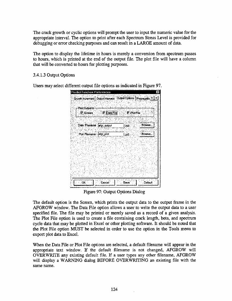
The crack growth or cyclic options will prompt the user to input the numeric value for the appropriate interval. The option to print after each Spectrum Stress Level is provided for debugging or error checking purposes and can result in a LARGE amount of data.
The option to display the lifetime in hours is merely a conversion from spectrum passes to hours, which is printed at the end of the output file. The plot file will have a column that will be converted to hours for plotting purposes.
3.4.1.3 Output Options
Users may select different output file options as indicated in Figure 97. (Predict Function Preferences E3
* Growth increment 1 Öutputlnteiväls ^Output Options j Prboaaafio ^1 ►
|p;F'FtfntÜijipuUt
-lie . . ■■]'.^Screen '•■■■ "" F/JDatalFilei .V'VVFsftotl
:ßx'-}'t.y: «/;j;SV-;"'fr^'^-^tvS :S
■ Browse... 1 :V:,'- Data fTilehar
Plot Fileriori
ne |afgr_output |[out ■■.-./ x
Browse_ ie . |afgr_plot jfepl2 <' c
.Default ' ■'
iOK Cancel ^Sovef-aX;
Figure 97: Output Options Dialog
The default option is the Screen, which prints the output data to the output frame in the AFGROW window. The Data File option allows a user to write the output data to a user specified file. The file may be printed or merely saved as a record of a given analysis. The Plot File option is used to create a file containing crack length, beta, and spectrum cycle data that may be plotted in Excel or other plotting software. It should be noted that the Plot File option MUST be selected in order to use the option in the Tools menu to export plot data to Excel.
When the Data File or Plot File options are selected, a default filename will appear in the appropriate text window. If the default filename is not changed, AFGROW will OVERWRITE any existing default file. If a user types any other filename, AFGROW will display a WARNING dialog BEFORE OVERWRITING an existing file with the same name.
124
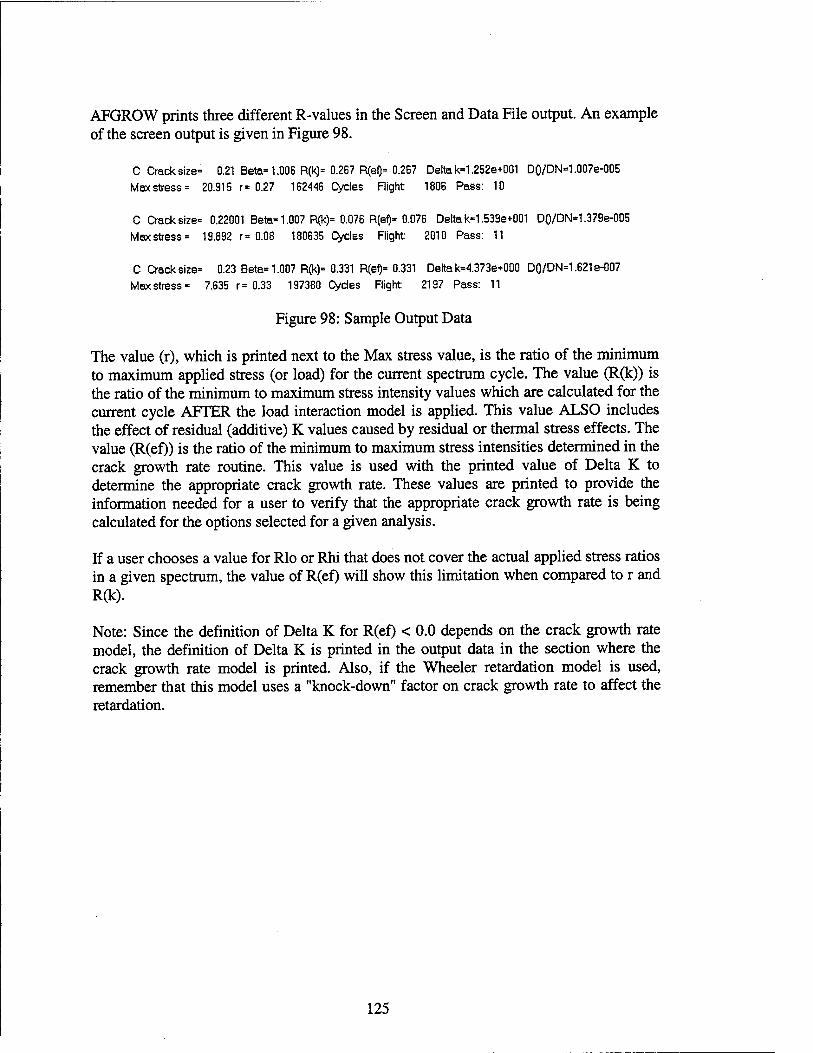
AFGROW prints three different R-values in the Screen and Data File output. An example of the screen output is given in Figure 98.
C Crack size= 0.21 Beta-1.006 R(k)= 0.267 R(ef)= 0.267 Delta k=1.252e+001 DQ/DN=1.007e-005
Max stress = 20.915 r= 0.27 162446 Cycles Flight: 1806 Pass: 10
C Crack size= 0.22001 Beta= 1.007 R(k)= 0.076 R(ef)= 0.076 Delta k=1.539e+001 D()/DN=1.379e-005
Max stress» 19.892 r= 0.08 180635 Cycles Flight: 2010 Pass: 11
C Crack size- 0.23 Bete-1.007 R(k)= 0.331 R(ei)= 0.331 Delta k«4.373e+000 DQ/DN=1.621e-007
Max stress- 7.635 r= 0.33 197380 Cycles Flight 2197 Pass: 11
Figure 98: Sample Output Data
The value (r), which is printed next to the Max stress value, is the ratio of the minimum to maximum applied stress (or load) for the current spectrum cycle. The value (R(k)) is the ratio of the minimum to maximum stress intensity values which are calculated for the current cycle AFTER the load interaction model is applied. This value ALSO includes the effect of residual (additive) K values caused by residual or thermal stress effects. The value (R(ef)) is the ratio of the minimum to maximum stress intensities determined in the crack growth rate routine. This value is used with the printed value of Delta K to determine the appropriate crack growth rate. These values are printed to provide the information needed for a user to verify that the appropriate crack growth rate is being calculated for the options selected for a given analysis.
If a user chooses a value for Rio or Rhi that does not cover the actual applied stress ratios in a given spectrum, the value of R(ef) will show this limitation when compared to r and R(k).
Note: Since the definition of Delta K for R(ef) < 0.0 depends on the crack growth rate model, the definition of Delta K is printed in the output data in the section where the crack growth rate model is printed. Also, if the Wheeler retardation model is used, remember that this model uses a "knock-down" factor on crack growth rate to affect the retardation.
125

3.4.1.4 Propagation Limits
AFGROW allows the user to set crack growth propagation limits on life analysis as indicated in Figure 99.
Predict Function Preferences
Output Intervals | Output Options Propagation Limits [Transitior < I >.
Stop Crock Propagation at-'.1- ~v. .■ f... "■>-'.-. " : T?: -
-i~j Crack Length; 9 ,
r Cycle Count
■ P-'--.' 'Kmax' Failure Criteria
r 'User-Defined 'Kmax"
17; ;'!NetSectJon Yield' FoilureCriteria'
I be repeated-
'!,' i SpectrumReps (Max.993999)r> > 1999999
-QIC' Caricel ''Save Default
Figure 99: Propagation Limits Dialog
When selected, AFGROW will terminate at the first instance of any selected limit. When a limit is selected which requires additional input, AFGROW will open the appropriate input box for data entry.
Note: In the case of the net section yield criteria, the net section stress is based on the remote tensile load and the net area in the crack plane (minus the yield zone).
Bearing load is assumed to be uniformly distributed through the net section and is determined as:
Bearing Load = Bearing Stress * Hole Diameter * Thickness
For cases that include out-of-plane bending, it would be far too conservative to use the bending stress value (taken at the plate surface). In this case, the tensile stress due to the bending at 1/6 of the thickness is substituted. This is the centroid of the tension stress due to the out-of-plane bending. The only exceptions to this are the rod and pipe geometries since the calculations are very complex since the change in moment of inertia would have to be recalculated as the crack grows. At this time, out-of-plane bending is ignored for these geometries in terms of net section stress.
126

AFGROW does not include any contributions of crack asymmetry to in-plane bending contributions to the net section stress. Although it is possible for in-plane bending to play a role in the true net section yielding, there are usually geometric constraints that will prevent or mitigate this effect.
3.4.1.5 Transition Options
AFGROW allows the user to set the part through to through-the-thickness crack transition criteria as indicated in Figure 100.
Predict Function Preferences
Output Options | Propagation Limits Transition Options
r-Transition to a Through Crack at -
i;R-S5%otthicknesspenetratiorjy
~ K.max in A direction greater or equal then effective ' fracture toughness (Kiel * , * .
OK Cancel SSave^ Default
Figure 100: Transition Options Dialog
These criteria control when a part-through crack becomes a through-the-thickness crack. The default transition criterion is 95 percent thickness penetration. When the a-dimension reaches 95% of the thickness (or 2a for surface or fully embedded cracks), the crack is assumed to become a through-the-thickness crack.
The alternative criterion is the Kk method. This has been used in NASGRO based on observations that transition may occur if the maximum stress intensity value in the a- direction exceeds a prescribed value. This value is called Kfc (equivalent fracture toughness for a part-thru crack). Values of Kie are included in the NASGRO material database. Typically, Kie may be estimated as:
KIe=1.4(KIc)
Kfc is (of course) the plane strain fracture toughness for a given material. Therefore, if the NASGRO material database is NOT used, Kfe will be estimated as shown above.
127
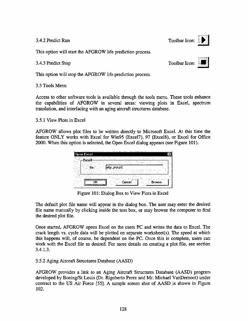
Toolbar Icon: |fj£
Toolbar Icon: I
3.4.2 Predict Run
This option will start the AFGROW life prediction process.
3.4.3 Predict Stop
This option will stop the AFGROW life prediction process.
3.5 Tools Menu
Access to other software tools is available through the tools menu. These tools enhance the capabilities of AFGROW in several areas: viewing plots in Excel, spectrum translation, and interfacing with an aging aircraft structures database.
3.5.1 View Plots in Excel
AFGROW allows plot files to be written directly to Microsoft Excel. At this time the feature ONLY works with Excel for Win95 (Excel7), 97 (Excel8), or Excel for Office 2000. When this option is selected, the Open Excel dialog appears (see Figure 101).
Open Excel
-Excel8-
file: afgr_plotpl2
OK Cancel Browse..
Figure 101: Dialog Box to View Plots in Excel
The default plot file name will appear in the dialog box. The user may enter the desired file name manually by clicking inside the text box, or may browse the computer to find the desired plot file.
Once started, AFGROW opens Excel on the users PC and writes the data to Excel. The crack length vs. cycle data will be plotted on separate worksheet(s). The speed at which this happens will, of course, be dependent on the PC. Once this is complete, users can work with the Excel file as desired. For more details on creating a plot file, see section 3.4.1.3.
3.5.2 Aging Aircraft Structures Database (AASD)
AFGROW provides a link to an Aging Aircraft Structures Database (AASD) program developed by Boeing/St Louis (Dr. Rigoberto Perez and Mr. Michael VanDernoot) under contract to the US Air Force [55]. A sample screen shot of AASD is shown in Figure 102.
128

EJ2E3M Alrcaratt Typ« JOB» Part Alrer»Ct
l"!lnf»1 7A*tuc«
3?
»«(•ntWR-AUOLJ
IS
OJM
0.1»
4
-4>m«* DimsmiMii);V «UBS
;"***?;
'■sUm'i
Figure 102: Aging Aircraft Structures Database
The AASD allows users to examine actual maintenance details and copy the crack data into the Windows clipboard for use in AFGROW. The AASD menu in AFGROW offers the following commands:
• Run - Run AASD • Paste-Paste data from AASD to AFGROW
Once the data are pasted into AFGROW, life predictions may be performed to estimate the life of a given component or to verify an analysis (if sufficient verification data are available in AASD).
This database provides detailed crack length, material and spectrum information for several current Air Force aircraft. The distribution of AASD may initially be limited. Requests to obtain a copy of AASD may be made through the Air Force (use the Mail command from the File menu). If AASD is not installed, this menu selection will be grayed out.
3.5.3 Run Spectrum Translator
AFGROW includes a spectrum translation program, Figure 103, which will convert many existing stress (or load) spectra to the format needed in AFGROW. This program is written and maintained by the developers of AFGROW (AFRI7VASE).
129

Gaiherihginformation- .-./•*,« •:.'",& -.-f Trtler11>07-199609:30:T4lnputRIe:UF_DTA.[WTFaA-i2t' SubSpedra:1Z40 MaxEydes: 63280 Max Stress: 3359 Miri.StressHBOY:; ''\/.:Y''"YMft'-Y'v'- ■•"■ YY:;Y
sBdt
jReed
Translate
^.
Figure 103: Spectram Translator
Currently, the following spectrum formats may be translated:
• Supercracks • Cracks 3 • NORCRAK • Cracks95
Once the spectrum has been read and analyzed, press the Translate button to finish the translation. The file names (filename.sp3 and filenameOl.sub) of the translated spectrum will be the same as the original file.
Other spectrum formats may be translated upon user request.
3.5.4 Run Cycle Counter
A cycle is defined as shown below in Figure 104. A cycle begins at a certain stress (or load) level, moves to a different level, and returns to the starting level.
Figure 104: Cycle Definition
Many people have submitted questions related to how AFGROW uses the input spectrum data. Each line in an AFGROW spectrum consists of one or more cycles. A cycle is described by any two of the following parameters: minimum value, maximum value, or stress ratio (R). It makes no difference which two parameters are used, or what order they are listed.
Real structures are loaded and unloaded periodically so that the peak-valley sequence of applied stresses is unlikely to form true cycles. The actual peak or valley points are often
130

referred to as reversals since the loading direction (increasing or decreasing) is reversed at each point (see Figure 105).
Reversal Spectrum
Figure 105: Sample Uncounted Stress Sequence
In any case, the important fact is that AFGROW assumes that the input spectrum is given in the form of cycles, not simply an uncounted sequence.
AFGROW provides a cycle counting program [XX] than can be used to convert uncounted sequences to cycles (see Figure 106). This tool is provided for the convenience of our users, but there are other cycle counting methods in the open literature that may be used as desired.
2<. Cycle Counting Program - Delta K Information Services. Inc.
file üiew Help . . .
;'^versal Information^
' Input Filename:
Reversals Stored in:
I Count Reversals: j- Reversals:■■y;0
*Sp*cfrum'Oütpüt;pie:?;F?
Sub-Spectra: 0
Spectrum Cycles: 0
Max Value Position : |ln Order "»]
P Normalize Spectrum
Count Spectrum jjjCancelJ Rainflow Counting Example
Figure 106: Cycle Counting Software Interface
131

This program has many features, which are described in detail in its own on-line help. The program will convert stress values to reversals and reversals to cycles. If reversals are available, they can be used as is to create the counted spectrum.
An important point to note is the placement of the maximum value in the spectrum. The cycle counting program will place counted cycles in the order determined by the order of the peak points. Some fracture mechanics experts prefer to place the overall maximum value at the end of the spectrum to minimize the effect on crack growth retardation (more conservative result). Others may prefer to place the maximum peak in the order that the peak occurs in the original sequence. There is an option to place the maximum value at the beginning, end, or in the original order of the peak values.
The resulting spectrum may be normalized so that the maximum value is 1.0. This is very common and allows users to scale the spectrum values based on the overall maximum value - without using a calculator.
Finally, it is important to know whether or not a spectrum has already been cycle counted. Generally, spectra created for crack growth life prediction will be counted. It is not easy to tell, so it is important to find out. If a counted spectrum is counted twice, it will be altered (unless it is a constant amplitude sequence). The initiation module in AFGROW assumes the spectrum is also counted (see section 3.7). It would have been very difficult to manage both counted and uncounted spectra in AFGROW. In short, if you are using a spectrum in AFGROW, it had better be cycle counted.
132

3.6 Repair Menu
AFGROW includes an option to account for the effect of a bonded repair patch on crack growth life. This analysis is based on a Green's function method and was developed by Dr. Mohan Ratwani [7]. Currently, this method is only valid for the following conditions:
• Through the thickness cracks • Thin structure (< 0.125 in.) • Non-stiffened panels • Crack remains under the patch
The stress intensity solution is determined by integrating the 2-D adhesive shear stresses in an area surrounding a centered through crack in an infinite plate. This area is simulated using a telescopic grid with a fine mesh covering the crack and a course mesh extending a distance of one half of the total crack length on either side. The height of the mesh extends to one and a half of the total crack length above and below the crack. Due to symmetry conditions, a quarter of the panel is analyzed with a total of 144 nodes. A unit stress is applied to the cracked panel and stress intensity values are determined for approximately 20 crack lengths (crack intervals are calculated using an algorithm in the model). The initial crack length is the same as the initial crack length specified by the user and the final crack size (c) does not exceed 2 inches. A beta correction table is generated by dividing the stress intensity for the patched case by the stress intensity for the same case without a patch. The correction for cracks exceeding 2 inches is assumed to be constant7. The assumption is that a centered through crack solution is used to determine the beta correction due to the bonded repair at various crack lengths and is applied to the actual geometry selected by the user. The 2-inch limit on the beta correction values is based on analysis and test verification data. These data indicate that the ratio of the patched to non-patched stress intensity values tend to be nearly constant above a half crack length (c) of 2 inches for the center cracked case using typical patch materials and adhesives.
AFGROW will store up to eight repair designs and their beta correction tables. The most current design is active by default, but the user may change the active design through the repair plot option in the view window or menu selection.
The repair menu options are described in the following sections.
3.6.1 Repair Design
When the repair design is selected, AFGROW will not allow certain values to be changed for the given crack model. The reason for this is that material properties and model dimensions are required for the repair analysis. If any of these values were changed, the
7 The stress intensity value will NOT be constant, only the beta correction value which is multiplied by the stress intensity value for the non-patched case
133

repair analysis would have to be redone. A dialog will appear informing users of this situation.
A wizard is used to guide users through the repair design process as described in the following sections.
3.6.1.1 Ply Design and Lay-up Ply Desiqn and Layup
-Material Properties -
Name: |GRAPHITE/EPOXi' .V]
|d".vi, 1 Value ■'■■■■;.:] Description 1 • EL "ET
■ 25000 Youngs... : 1500 Youngs... #
GLT PNU
: 700 ..Shear M... ! : 0.3 Poisson... &:■
Ai_a ALFT
, ^BHU07 Coef.of... ';■ : 28-005 Coef.of... ?
Change MaterialDatabaseBle | :
"Number of .Plies: -"" :ll 3,': ~»; - ' -H
' PlyTbickness:5^0.0052
::OeltatS::%|0~
"Pry Layup:
Oriental ■ Pty#-f !
A 45 1 A -45 A 0
2 3
A 0 A 90
4 5 '
A 0 A 0 ■"
E ' 7
A 0 i 8 A 90 ;
Zl 7 A 0 " Z"-45'"'
9 10
~" 11 12
A 45 13
p Patch Type
Number of Plies is half the total numbers of plies for symmetric !
Kpotches:;w:c!'^.N-J^'V
.»CrSymmetric ;*:(■,,
njDoüble^ided;; -
*I~'No Bending. \
»Patch Sfiffness Ihdicotbrpi of Plate Stiffriess).'
■'i: l
Out of bounds'.:
70% ■■•'I-.'"'
Allowed IdeaJ Allowed
450% ''■V :■* :■!'■
VOut of bounds
;Auto.Desigrt <Bac* .Next» ' Cancel -Help;
Figure 107: Ply Design and Lay-up Dialog
This dialog contains the information for the repair patch including whether to consider out of plane bending and an option to consider thermal residual stresses in the stress intensity solution. The repair design is performed automatically using an internal algorithm based on the maximum applied stress and the modulus of the cracked plate. The automatically generated ply lay-up includes cross plies to provide delamination resistance. In addition, Dr Ratwani's method tends to produce errors if the patch moduli in the x and y directions differ greatly. For these reasons, cross ply lay-ups are preferred. The load direction is assumed to be normal to the crack plane. Users can make any desired changes to the design by making changes to the material properties, ply lay-up, or type of patch.
3.6.1.1.1 Material Properties
The material properties are given for the appropriate material in the default database file. The user MAY NOT change these values since they are interrelated. The use of invalid
134

composite material properties will cause the analysis to crash. Users may create their own material database files8, but must be sure to input valid property values.
The user has control over the number of plies, ply thickness, and Delta T. The Delta T parameter (degrees F) is included to provide a means to account for the residual thermal stressed caused by the differences between the thermal expansion of the cracked plate and composite patch. Some believe that Delta T should be the difference between the patch curing temperature and the operating temperature. Others think that there may be some relaxation in the adhesive after curing which results in a lower effective Delta T. In any case, the user is free to use judgment in setting this value.
3.6.1.1.2 Ply Lay-up
The ply lay-up is initially determined by AFGROW based on a criterion to include cross plies for some biaxial strength, symmetry, and a target value of patch stiffness of 110 percent of the cracked plate stiffness. The user may change the lay-up9 by using the mouse to either drag a ply to a new location or selecting a ply (single click) and touching the control key (or a second, single mouse click after a few second pause). AFGROW also includes an option to auto design the ply orientation (left click in the Orient... button) and an auto design option for both the orientation and number of plies (left click in the Ply # button). Cross ply lay-ups are desirable to help prevent the patch from delaminating during normal use. Also, it should be noted that Dr. Ratwani's method has been known to have problems if the patch Ex and Ey values differ by large amounts (i.e.: uniaxial lay-up).
3.6.1.1.3 Patch Type
The three options for patch types are:
Symmetric: The ply lay-up shown is doubled and the lay-up is therefore symmetric with respect to the center of the patch.
Double Sided: The patch is applied on both sides of the cracked plate (eliminates out of plane bending for symmetric patches).
No Bending: Do not account for out of plane bending in the calculations. The plate may be constrained to prevent bending or the user may wish to compare the results with and without out of plane bending.
8 The data in the material database file must be in English units. AFGROW will make the appropriate conversion based on the current units being used. 9 The maximum number of allowable plies in the current version is 32 (16 if the symmetric option is active).
135

3.6.1.1.4 Patch Stiffness Indicator
The patch stiffness indicator allows the user instant feedback on the patch design. The target is 110 percent of the plate stiffness to provide strength to help keep the crack closed, but not so stiff to attract too excessive load to the patch. Remember that this is calculated based on thickness and is independent on the patch width. Where possible, it is recommended that the patch width be twice the width of the crack over the projected life of the repair.
3.6.1.2 Patch Dimensions and Adhesive Properties
This dialog, Figure 108, contains the information for the repair patch dimensions and adhesive properties. This includes modeling the local disbond in the adhesive, which tends to occur around a cyclically loaded crack. There is also an option to control whether the patch is considered when using the critical stress-intensity factor failure criterion.
IPatch Dimensions and Adhesive Properties
k'.'^k ,.^">>\^..'!:"■■; ->'"' ; K .;. ':■ " -'• v
Name: J
Shear Moc
Thickness
Disbond ([
";'•, =W-73| ■f'..
i ;;'■'' ■*■.''
;;.J^m^' ■ ■
1 -'
lulus (G*0: |60
Dh 1 111 H i—m gSjW B» a. ■ ■ ... T . Mw ■■«■ -_i
. :7V jo.oos
IS wq-. |o
.'-" ■ ■'
dth(Wp): \A ^DlBSHMÜ c |r v
ngth(Lp): \A
.-' ' '
-^-.■^L::;J-J„- •
»L f-H 1 III' S"A
■fez -^-^-"JH f Patched Structure .
. Wp " . .- r Unpatched Structure
■':-'•.- '■' ":'.-
s.;,;...-, • '■■" . ■- '■ "" i-:'-.'' ''':' ■=■'■' -■'■•'•,■ '.'■"' '.' ' . '• ' ;
;iV -' ~. :•■■ '.-.'■ >''- -.' :':-';v '■'■' ' ■:',':- '^ : ::' .'' ~..-. ■' ' •
Help |#:i/:;: K^ Vv;.'V;;"> "«SÖidc; ; Uext> ■' -Cancel - j |
Figure 108: Patch Dimensions and Adhesive Properties Dialog
3.6.1.2.1 Sample C-Scan Image of a Repair
The sample C-Scan image (see Figure 108) is provided to show the patch dimensions and explain the concept of the adhesive disbond, which normally occurs around the crack tip under cyclic loading. The method, proposed by Dr Ratwani, assumes the disbond follows the crack tip and is elliptical in shape.
136
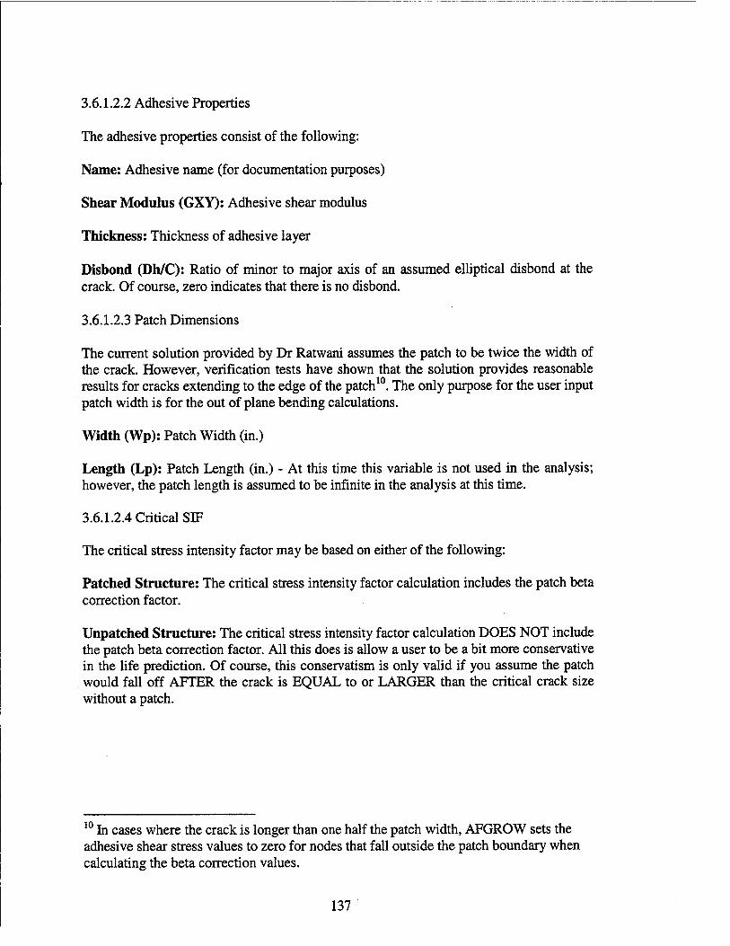
3.6.1.2.2 Adhesive Properties
The adhesive properties consist of the following:
Name: Adhesive name (for documentation purposes)
Shear Modulus (GXY): Adhesive shear modulus
Thickness: Thickness of adhesive layer
Disbond (Dh/C): Ratio of minor to major axis of an assumed elliptical disbond at the crack. Of course, zero indicates that there is no disbond.
3.6.1.2.3 Patch Dimensions
The current solution provided by Dr Ratwani assumes the patch to be twice the width of the crack. However, verification tests have shown that the solution provides reasonable results for cracks extending to the edge of the patch10. The only purpose for the user input patch width is for the out of plane bending calculations.
Width (Wp): Patch Width (in.)
Length (Lp): Patch Length (in.) - At this time this variable is not used in the analysis; however, the patch length is assumed to be infinite in the analysis at this time.
3.6.1.2.4 Critical SIF
The critical stress intensity factor may be based on either of the following:
Patched Structure: The critical stress intensity factor calculation includes the patch beta correction factor.
Unpatched Structure: The critical stress intensity factor calculation DOES NOT include the patch beta correction factor. All this does is allow a user to be a bit more conservative in the life prediction. Of course, this conservatism is only valid if you assume the patch would fall off AFTER the crack is EQUAL to or LARGER than the critical crack size without a patch.
10 In cases where the crack is longer than one half the patch width, AFGROW sets the adhesive shear stress values to zero for nodes that fall outside the patch boundary when calculating the beta correction values.
137

3.6.1.3 Designed Patch Properties
This dialog, Figure 109, shows the ply lay-up and resulting laminate structural properties. Designed Patch Properties
:Pty Orientations- -Patch Properties- -TT——r-—^———-— ■ ;.:.■
< Name: ' |GRAPHITE/EPO
Youngs Modulus mXDir. (EX):
Youngs Modulus in Y Dir. (EY):
Shear Modulus (GXY): *
.', Thickness (THICK):
XY Poisson Ratio (NUXV):
, YX Poisson Ratio (IMUYX):
_ Coef. of Thermal Exp. in Yc >
>CoetofT>iermalExp. inX:
WdthVp):
," LengtH.(Lp): ' /:•''■';>,■;■-■..
XY -
|15400.3886718 • ■
|6708.3B ;
J2464.54 • ■....:
. {0.0676
|0:316096 •
|0:137691 :
|l.3414e^07 .'',:
. J2 87297B-006 :
'K . . ■:;.
H •
Save <Bock' tje»t> j Cancel Help
Figure 109: Patch Dimensions and Adhesive Properties Dialog
Ply Orientations: This window simply shows the ply orientation of the complete patch.
Patch Properties: The patch properties are given for the total patch laminate.
Save Button: The complete repair design may be saved to a file for later use.
At this point, clicking on the NEXT button will start the repair analysis. This can take a few minutes (depending on the computer) and a progress bar will appear to give an indication of the expected run time.
Once the analysis is complete, the repair beta correction vs. crack length plot is displayed, as shown in Figure 110.
138
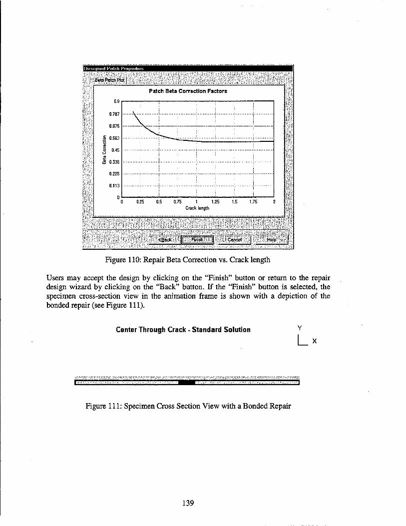
Designed Patch Properties
SBewPatefrPIc*
Patch Beta Correction Factors
0.9
075 1 1.25 Crack length
<fiack |i JRnish jj Cancel j üfcleiftö
Figure 110: Repair Beta Correction vs. Crack length
Users may accept the design by clicking on the "Finish" button or return to the repair design wizard by clicking on the "Back" button. If the "Finish" button is selected, the specimen cross-section view in the animation frame is shown with a depiction of the bonded repair (see Figure 111).
Center Through Crack - Standard Solution Y
Figure 111: Specimen Cross Section View with a Bonded Repair
139
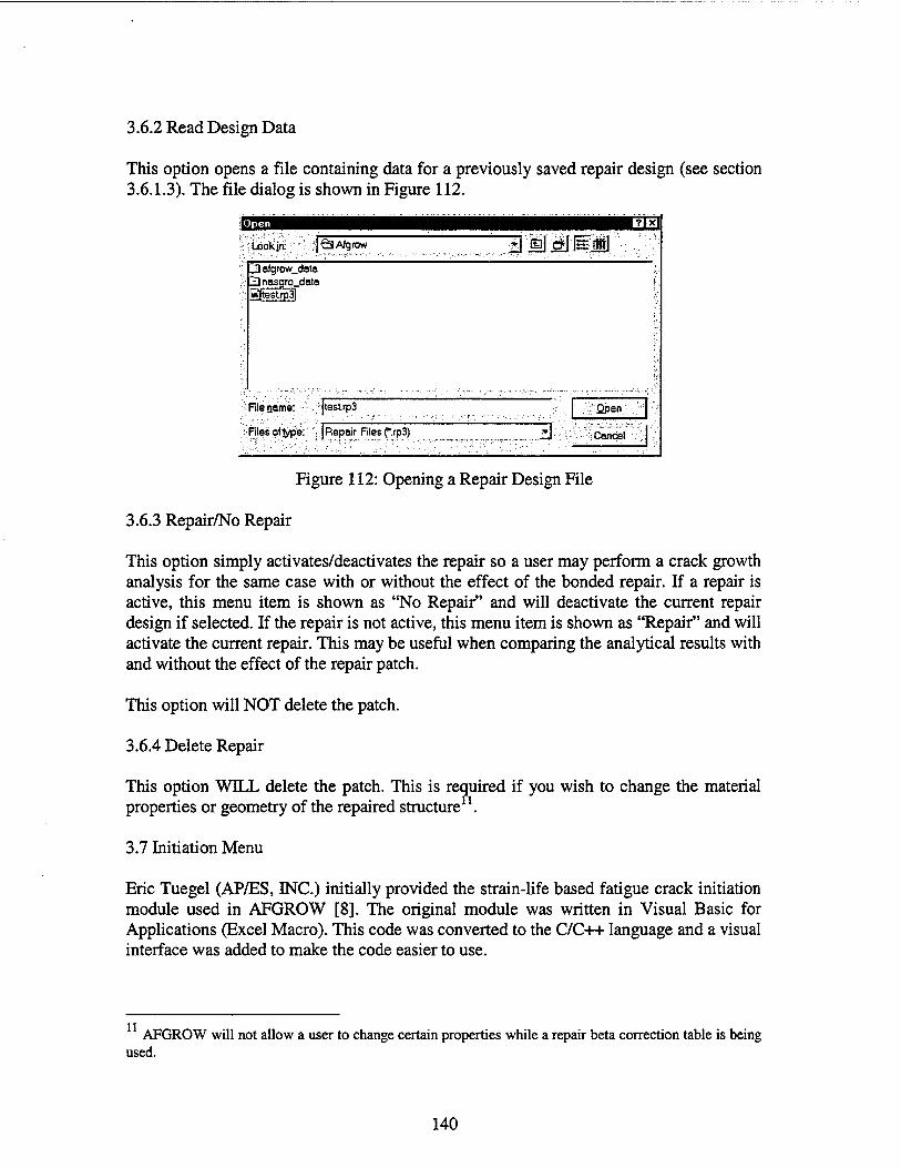
3.6.2 Read Design Data
This option opens a file containing data for a previously saved repair design (see section 3.6.1.3). The file dialog is shown in Figure 112.
BBffll fWxl
-Lookin: I^Afgrow H j£ji dji i^isi _3 afgrow_data Zünasgro data @teitip3l
Hie name: |testrp3 'Qpsn
: Files pflype: ■': |Repair_Filesf.rp3) ~ _ F] Cancel
Figure 112: Opening a Repair Design File
3.6.3 Repair/No Repair
This option simply activates/deactivates the repair so a user may perform a crack growth analysis for the same case with or without the effect of the bonded repair. If a repair is active, this menu item is shown as "No Repair" and will deactivate the current repair design if selected. If the repair is not active, this menu item is shown as "Repair" and will activate the current repair. This may be useful when comparing the analytical results with and without the effect of the repair patch.
This option will NOT delete the patch.
3.6.4 Delete Repair
This option WILL delete the patch. This is required if you wish to change the material properties or geometry of the repaired structure .
3.7 Initiation Menu
Eric Tuegel (AP/ES, INC.) initially provided the strain-life based fatigue crack initiation module used in AFGROW [8]. The original module was written in Visual Basic for Applications (Excel Macro). This code was converted to the C/C++ language and a visual interface was added to make the code easier to use.
AFGROW will not allow a user to change certain properties while a repair beta correction table is being used.
140
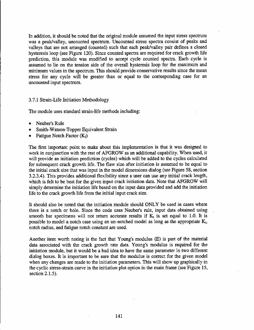
In addition, it should be noted that the original module assumed the input stress spectrum was a peak/valley, uncounted spectrum. Uncounted stress spectra consist of peaks and valleys that are not arranged (counted) such that each peak/valley pair defines a closed hysteresis loop (see Figure 120). Since counted spectra are required for crack growth life prediction, this module was modified to accept cycle counted spectra. Each cycle is assumed to lie on the tension side of the overall hysteresis loop for the maximum and minimum values in the spectrum. This should provide conservative results since the mean stress for any cycle will be greater than or equal to the corresponding case for an uncounted input spectrum.
3.7.1 Strain-Life Initiation Methodology
The module uses standard strain-life methods including:
• Neuber's Rule • Smith-Watson-Topper Equivalent Strain • Fatigue Notch Factor (Kf)
The first important point to make about this implementation is that it was designed to work in conjunction with the rest of AFGROW as an additional capability. When used, it will provide an initiation prediction (cycles) which will be added to the cycles calculated for subsequent crack growth life. The flaw size after initiation is assumed to be equal to the initial crack size that was input in the model dimensions dialog (see Figure 58, section 3.2.3.4). This provides additional flexibility since a user can use any initial crack length, which is felt to be best for the given input crack initiation data. Note that AFGROW will simply determine the initiation life based on the input data provided and add the initiation life to the crack growth life from the initial input crack size.
It should also be noted that the initiation module should ONLY be used in cases where there is a notch or hole. Since the code uses Neuber's rule, input data obtained using smooth bar specimens will not return accurate results if Kt is set equal to 1.0. It is possible to model a notch case using an un-notched model as long as the appropriate Kt, notch radius, and fatigue notch constant are used.
Another item worth noting is the fact that Young's modulus (E) is part of the material data associated with the crack growth rate data. Young's modulus is required for the initiation module, but it would be a bad idea to have the same parameter in two different dialog boxes. It is important to be sure that the modulus is correct for the given model when any changes are made to the initiation parameters. This will show up graphically in the cyclic stress-strain curve in the initiation plot option in the main frame (see Figure 15, section 2.1.5).
141

3.7.1.1 Neuber's Rule
Neuber's equation [55] may be expressed in the following form:
(Kf*s)2 _A<rAe (4E) 2
Where S is the applied stress and a and E are the resulting local stress and strain values corrected for the notch effect.
Since the local corrected stress and strain values are two unknown values; the input material cyclic stress strain curve is used in conjunction with Neuber's equation to determine these values as indicated in Figure 113.
Neuber's Equation
Figure 113: Neuber's Rule
3.7.1.2 Smith-Watson-Topper Equivalent Strain
Normally, strain-life data are available for the case of fully reversed loading (R = -1.0). In order to account for the effect of load cycles that are not fully reversed, an equivalent applied strain must be determined for each cycle in the applied spectrum. The Smith, Watson, and Topper equivalent strain equation [57] is probably the most common method used to convert the strain amplitude for a given load cycle to the equivalent fully reversed strain amplitude. The equation may be expressed in the following form:
Ae 2 eq
Where, S is the applied stress, s is the applied strain, and E is Young's Modulus for the material
142
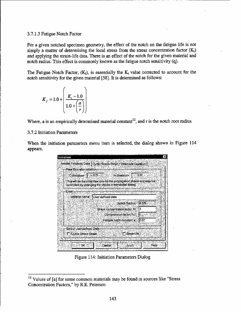
3.7.1.3 Fatigue Notch Factor
For a given notched specimen geometry, the effect of the notch on the fatigue life is not simply a matter of determining the local stress from the stress concentration factor (Kt) and applying the strain-life data. There is an effect of the notch for the given material and notch radius. This effect is commonly known as the fatigue notch sensitivity (q).
The Fatigue Notch Factor, (Kf), is essentially the Kt value corrected to account for the notch sensitivity for the given material [58]. It is determined as follows:
£,=1.0 + £,-1.0
1.0 + \rj
Where, a is an empirically determined material constant12, and r is the notch root radius
3.7.2 Initiation Parameters
When the initiation parameters menu item is selected, the dialog shown in Figure 114 appears.
Initiation
Model / Material Data J Cyclic Stress-Strain /Strain Life Equation j
r Flaw Size after initiation :—: ; '—• =
C direction- 0.01 Indirection? yOJQi;
This will be the initial flaw size for the propagation phase and may be controlled by changing the values in the Model dialog.
pEnter- .—_
Material name- jUser defined data •liff'
. ". Notch Radius:
Stress concentration factor. Kt
Compression factor. Kc':
Fatigue notch constant a:.
0.125
3
|1 . -.
|0.02
r Select User defined Data-
r~ Cyclic Stress-Strain r Strain Lrfe
:OK'; Cancel - 6PPV 'Help5'
Figure 114: Initiation Parameters Dialog
12 Values of [a] for some common materials may be found in sources like "Stress Concentration Factors," by R.E. Peterson
143

The parameter dialog is divided into two categories:
• Model/Material Data • Cyclic Stress-Strain / Strain-Life Equation
AFGROW also includes an option to enter tabular stress-strain or strain-life data. These data are described in more detail in the following sections.
3.7.2.1 Model/Material Data
The model/material data dialog is shown in Figure 114.
Notch Radius (r); Physical radius of local notch (or hole) which is causing a local stress concentration.
Stress Concentration Factor (Kt): Stress concentration factor CTiocai/CTref.
Compression Factor (Kc); Determines the amount of the applied compressive stress (fraction of applied tension) to be used in the initiation analysis - not currently active.
Fatigue Notch Constant (a): Material constant used to determine the Fatigue Notch Factor, Kf.
3.7.2.2 Cyclic Stress-Strain / Strain-Life Equation
Initiation
Model / Material Data Cyclic Stress-Strain / Strain Life Equation
cmer .<.-.-. .-...-■
Cyclic Stress-Strain Equation: x=ff+(§£-]*'
Strain UfeEquation: ^=|ü|Ej (2N,)b+EPSF(2N,f
•■ ■ ■..■■■■■■'
^| ■-.-': Cyclic strength coefficient K': ; 74
Cyclic strain hardening exponent n': ■ 0.032
Fatigue strength coefficient S|GF:
Fatigue strength exponent b:
Fatigue ductility coefficient EPSF:
116
-0.098
0.26
: Fatigue ductility exponent c: j-0.73
OK Cancel APPV Help
Figure 115: Cyclic Stress-Strain / Strain-Life Equation Dialog
144
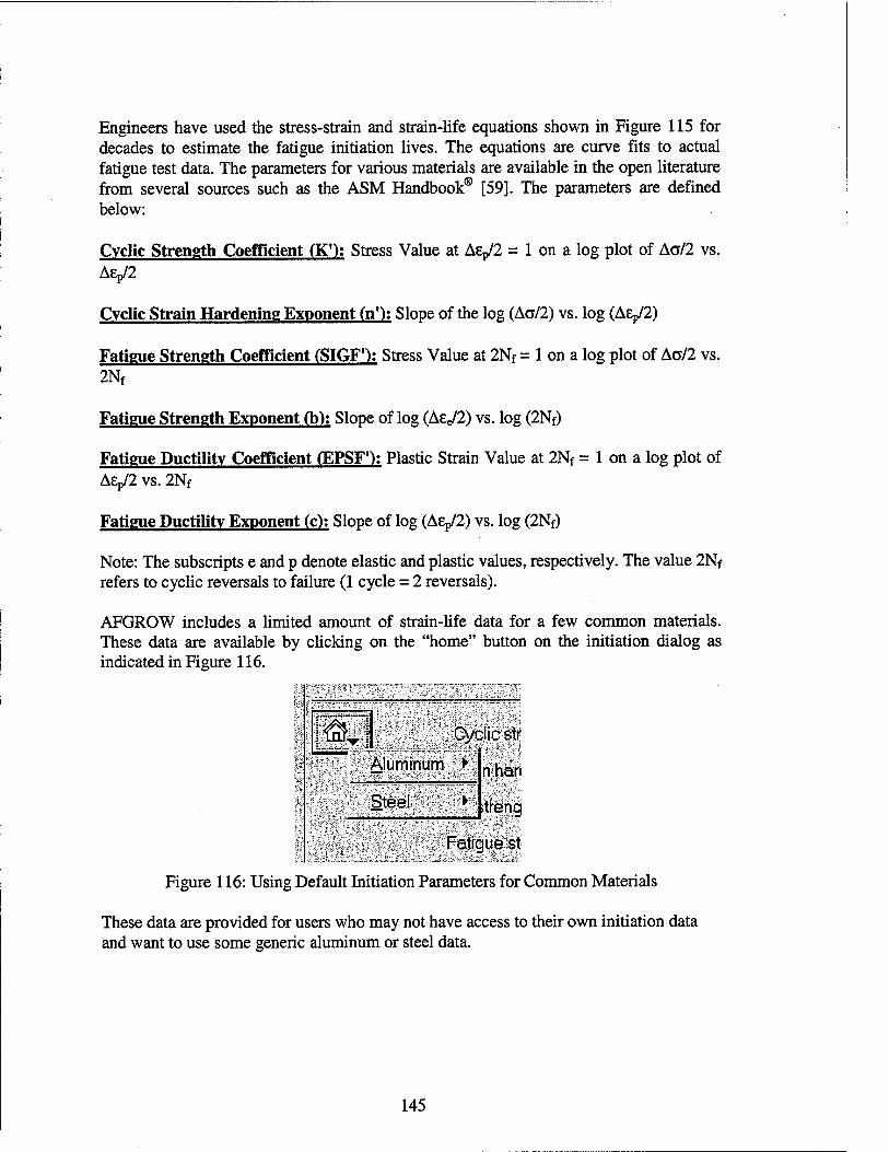
Engineers have used the stress-strain and strain-life equations shown in Figure 115 for decades to estimate the fatigue initiation lives. The equations are curve fits to actual fatigue test data. The parameters for various materials are available in the open literature from several sources such as the ASM Handbook® [59]. The parameters are defined below:
Cyclic Strength Coefficient (K'): Stress Value at A8p/2 = 1 on a log plot of Aa/2 vs. ÄEp/2
Cyclic Strain Hardening Exponent (n'); Slope of the log (Aa/2) vs. log (AEp/2)
Fatigue Strength Coefficient (SIGF')i Stress Value at 2Nf = 1 on a log plot of Aa/2 vs. 2Nf
Fatigue Strength Exponent (b): Slope of log (AE</2) VS. log (2Nf)
Fatigue Ductility Coefficient (EPSF1): Plastic Strain Value at 2Nf = 1 on a log plot of A8p/2 vs. 2Nf
Fatigue Ductility Exponent (c); Slope of log (A8p/2) vs. log (2Nf)
Note: The subscripts e and p denote elastic and plastic values, respectively. The value 2Nf refers to cyclic reversals to failure (1 cycle = 2 reversals).
AFGROW includes a limited amount of strain-life data for a few common materials. These data are available by clicking on the "home" button on the initiation dialog as indicated in Figure 116.
Cyclic str
Aluminum ►
Steel
nhan
streng
Fatigue st
Figure 116: Using Default Initiation Parameters for Common Materials
These data are provided for users who may not have access to their own initiation data and want to use some generic aluminum or steel data.
145

3.7.3 User-Defined Cyclic Stress-Strain / Strain-Life Data
A user may choose to enter the Cyclic Stress-Strain data and/or the Strain-Life data in tabular form. The choice is controlled by the following check box controls in the initiation parameter dialog shown in Figure 117.
-Select User defined Data' ~-v,.r-
^Cyclic Stress-Strain |7 jStrain Lifej
Figure 117: Options for User Defined Initiation Data
A new tab will appear for each box that is selected as shown in Figure 118.
Model / Material Data. CyclicStress-StrainTJata Strain Life Data]
Figure 118: Options for Stress-Strain and Strain-Life Input Data
The data must be entered in tabular format by selecting the appropriate tab. These data may be pasted from Excel or entered in the grid control by hand.
3.7.3.1 Cyclic Stress-Strain Data
JMpdeiy MätejalDäta] Sb^OfeEquifai: "C^Sbe^SliamData j
"' The cycScsbess-strain curve is determine by connecting the positive! : stress tjpsof the stable hysterisis curve for a given material The initial
slope of the curve should be equal toYoung's modulus.
Enter up to 25 values-
Read
Number of Sets: ,.|2Ö~3
Save
Copy
Eäste
Set;,."~-^:: Strain '.'-:• Stress ▲
O"'-;;;;.^.'-,; o",:-: ■:-■■:"■;-:■. O-'-J..;-;---'-' 1\.;™ '■■■■■/ W£A& £48
1296 7'::■ ■■ ,::■-■ 0.0O123 3 '?';&:■:•. '■■■, 0.00185 19.44 A ?>■:::■.:.■:: ■ 0.0025 25.92 5'-■•;■-M?, : 0.0031 32.4 6'■■-■■■.■-,■■:■■:■ r;..:.■ 0.0037 38.88 7''.■■;■"■■::'.-.■;■' 0.0043 45.36 zl
OK ; Cancel; L&ppb'; -Help:
Figure 119: User-Defined Cyclic Stress-Strain Data
Cyclic stress-strain data are obtained from fully reversed cyclic load tests. These tests are conducted at several load levels where stress vs. strain data are obtained and monitored until the hysteresis curve (map of stress vs. strain for each cycle) becomes stabilized. The cyclic stress-strain curve is the locus of the tips of the stable hysteresis curves in the positive stress and strain quadrant of the plot (see Figure 120).
146
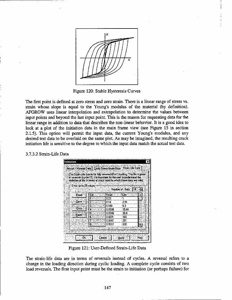
I I I I I i
Figure 120: Stable Hysteresis Curves
The first point is defined at zero stress and zero strain. There is a linear range of stress vs. strain whose slope is equal to the Young's modulus of the material (by definition). AFGROW uses linear interpolation and extrapolation to determine the values between input points and beyond the last input point. This is the reason for requesting data for the linear range in addition to data that describes the non-linear behavior. It is a good idea to look at a plot of the initiation data in the main frame view (see Figure 15 in section 2.1.5). This option will permit the input data, the current Young's modulus, and any desired test data to be overlaid on the same plot. As may be imagined, the resulting crack initiation life is sensitive to the degree to which the input data match the actual test data.
3.7.3.2 Strain-Life Data
Model / Material Data ] Cyclic Stress-Strain Data Strain Life Data ]
.-'The Strain-Life data is for fuUy reversed J.R=-.1) loading. The Efe is given ■. in reversals (cycles'?). It is important for the user to understand the - /«definition of fife fin terms of crack size) for which these data are valid, i
fEnter tip to25 values-;
':fieadi;
sSave,'
!©DRS
Miastet
Number of Sets: |18 & Set Strain | Life ',±'
1 ~ 0.23 ; 1 '■2" ,- ',■ '■■ 0.14 ;251 i,-f- 3' • -..V 0.086 S 3 4 0.0539 i 15.84 5;Iir#Jif 0.0348 139.8 fs~. 8 . "- - 0.0231 ! 100 '0~ 7 0.0161 |251 8' ''■'■■','-.■ 0.0117 1630 IzJ ;^£^^™:~^
?ÖK? Cancel jSppiy" ,HelK
Figure 121: User-Defined Strain-Life Data
The strain-life data are in terms of reversals instead of cycles. A reversal refers to a change in the loading direction during cyclic loading. A complete cycle consists of two load reversals. The first input point must be the strain to initiation (or perhaps failure) for
147

one reversal (monotonic loading). AFGROW uses logarithmic interpolation and extrapolation to determine the values between input points and beyond the last input point. The reason for this is to avoid any case where a negative strain value could result from an interpolation or extrapolation. It was also determined that logarithmic interpolation results in most accurate results. The resulting crack initiation life tends to be VERY sensitive to the degree in which the input data matches the actual test data. It is v. good idea to look at a plot of the initiation data in the main frame view (see Figure 15 in section 2.1.5). This option will overlay the input data and any desired test data. As noted in the dialog, IT IS VERY IMPORTANT for the user to know the definition of life13 for the input data. This definition should be used in the initial crack length, which is input by the user for subsequent crack growth analysis. AFGROW will determine an initiation life from the input data and proceed with a crack growth analysis from the initial crack length(s) entered for the given problem.
3.7.4 Initiation/No Initiation
This option simply activates/deactivates the initiation analysis so a user may perform a life analysis for the same case with or without including the initiation life. If the initiation option is active, this menu item is shown as "No Initiation" and will deactivate the initiation analysis if selected. If the initiation option is not active, this menu item is shown as "Initiation" and will activate the initiation analysis. This may be useful when comparing results with and without including the time to crack initiation.
3.8 Window Menu
The three frames, discussed in detail in sections 2.1, 2.2, and 2.3, make up the views for the life prediction analysis. To allow the largest view of the spectrum when the view, spectrum plot option is selected (see Figure 90, section 3.3.9), the entire AFGROW window is used to display the spectrum. The window menu is used to control the display of the spectrum and the three AFGROW frames.
Window belp
Cascade Tile
*1 Predict Datal 2Spectrum1
Figure 122: Window Menu
13 Crack length assumed as the definition of crack initiation
148
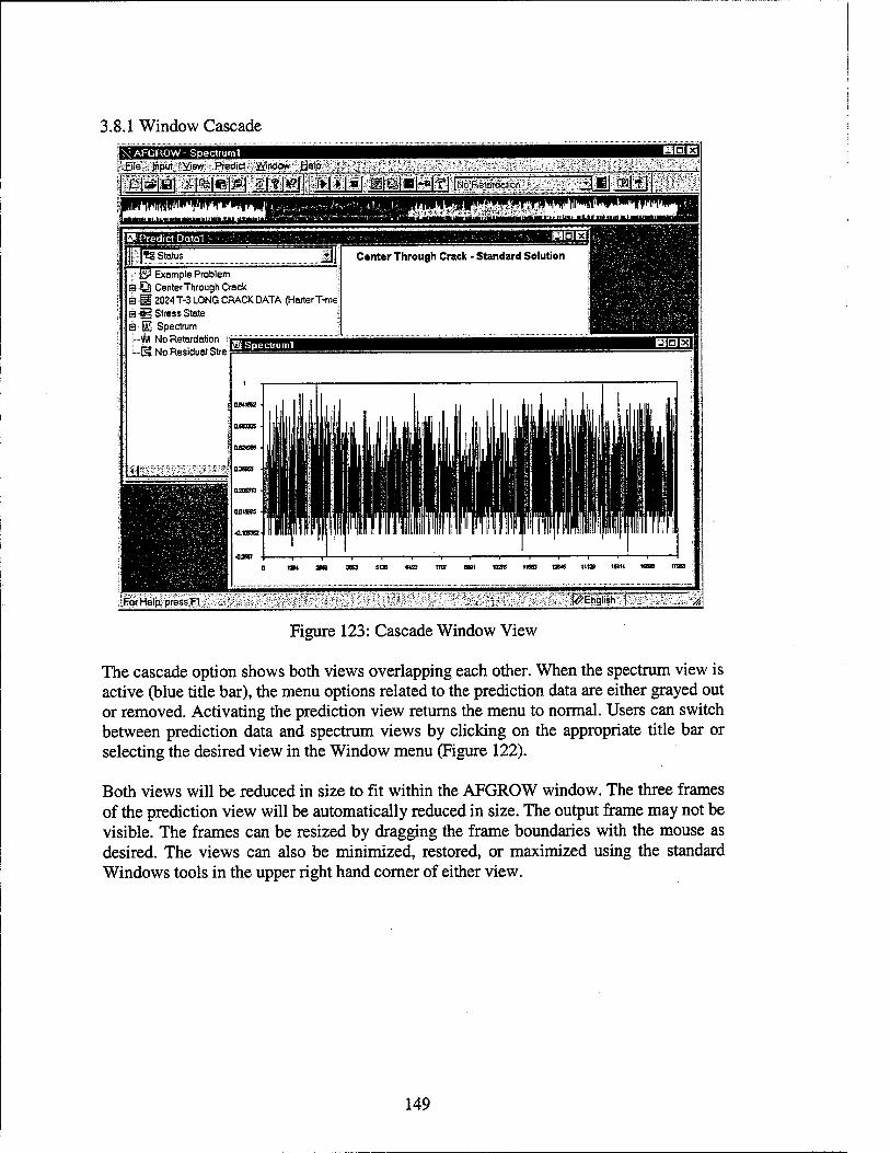
3.8.1 Window Cascade ><AFGROW-Spectruml Ißle input Yiew Predict Window jjelp-
DlsSlal SfolBlPl B|f|>g|; l»l»l"l aBlMH^llNTteariatoft; 11 ■! mit!
Mi miiiiMimmmiii m iitmm
FBtiPff»l,ll'"l"rrii|il^wi^'"Mli|li|nPiiji|
: .,-.-,., ■-.;...„ i.~ .... mi im, IM|1I HDiiffl 11 imniiiiMimBi
W Predict Data!
Ijlg Status
;- IP Example Problem j: B-^ CenterThrough Crack j $-3 2024 T-3 LONG CRACK DATA (HarterT-mq g-Sg Stress State S B Spectrum
i # No Retardation i-K No Residual Stre!
Center Through Crack - Standard Solution
SiS Spectruml
|rSrHelpifpress;R, ^English;
Figure 123: Cascade Window View
The cascade option shows both views overlapping each other. When the spectrum view is active (blue title bar), the menu options related to the prediction data are either grayed out or removed. Activating the prediction view returns the menu to normal. Users can switch between prediction data and spectrum views by clicking on the appropriate title bar or selecting the desired view in the Window menu (Figure 122).
Both views will be reduced in size to fit within the AFGROW window. The three frames of the prediction view will be automatically reduced in size. The output frame may not be visible. The frames can be resized by dragging the frame boundaries with the mouse as desired. The views can also be minimized, restored, or maximized using the standard Windows tools in the upper right hand corner of either view.
149
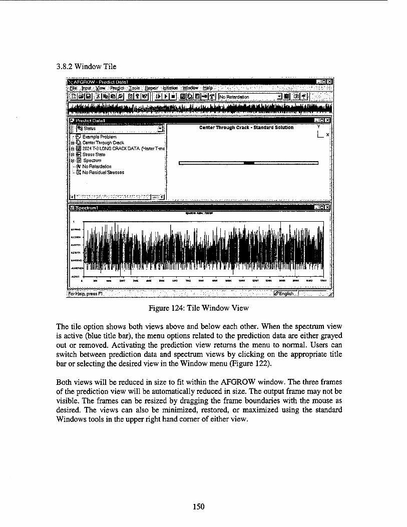
3.8.2 Window Tile
~N; AFGROW - Predict Datal ffile Input yisw Predict vlools Bepair Initiation Window flelp
ipfsfBl^l @| f #| l^^täi.älBlENIyilNo^tenJriSrr läwmm
W Predict Datal
j;:'J*8 Status ~j|
:-EP Example Problem B--ö Center Through Crack Ä ü 2024 T-3 LONG CRACK DATA (Harter T-md a g Stress State S-l Spectrum
i•-# No Retardation ~S No Residual Stresses
USEU
Center Through Crack - Standard Solution Y ;.
Lxl;
[JSSpectruml ^tcnmumf.nmm
• M*
For Help, press Fl (^English ,r
Figure 124: Tile Window View
The tile option shows both views above and below each other. When the spectrum view is active (blue title bar), the menu options related to the prediction data are either grayed out or removed. Activating the prediction view returns the menu to normal. Users can switch between prediction data and spectrum views by clicking on the appropriate title bar or selecting the desired view in the Window menu (Figure 122).
Both views will be reduced in size to fit within the AFGROW window. The three frames of the prediction view will be automatically reduced in size. The output frame may not be visible. The frames can be resized by dragging the frame boundaries with the mouse as desired. The views can also be minimized, restored, or maximized using the standard Windows tools in the upper right hand corner of either view.
150
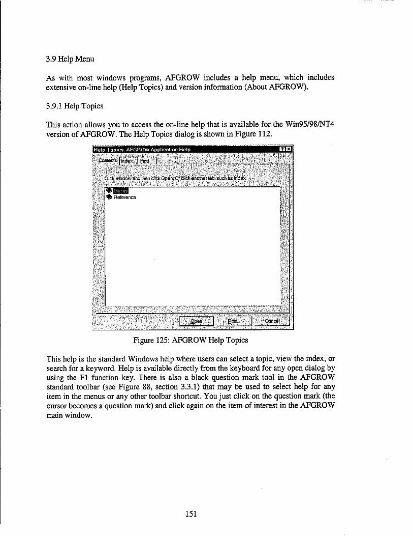
3.9 Help Menu
As with most windows programs, AFGROW includes a help menu, which includes extensive on-line help (Help Topics) and version information (About AFGROW).
3.9.1 Help Topics
This action allows you to access the on-line help that is available for the Win95/98/NT4 version of AFGROW. The Help Topics dialog is shown in Figure 112.
Help Topics: AFGROW Application Help
Contents [index | Find |
Dick a book, and then click Open. Or dick another tab. such as Index.
> Reference
Open ::Eriht!f Cancel
Figure 125: AFGROW Help Topics
This help is the standard Windows help where users can select a topic, view the index, or search for a keyword. Help is available directly from the keyboard for any open dialog by using the Fl function key. There is also a black question mark tool in the AFGROW standard toolbar (see Figure 88, section 3.3.1) that may be used to select help for any item in the menus or any other toolbar shortcut. You just click on the question mark (the cursor becomes a question mark) and click again on the item of interest in the AFGROW main window.
151
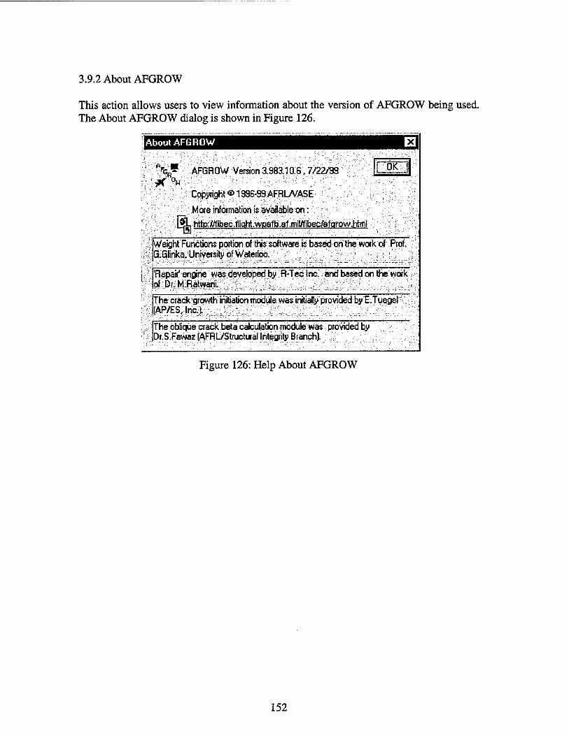
3.9.2 About AFGROW
This action allows users to view information about the version of AFGROW being used. The About AFGROW dialog is shown in Figure 126.
About AFGROW
AfGf* AFGROW Version 3,983.10.6.7/22/35 "ÖK" :X°w
^Copyright ©1996-99 AFRüVASE ;
More information is available on:
l^L http://fibec.fyqht.wpafb.af.mil/fibec/afqrowhtml
Weight Functions portion of this software is based on the work of Prof. G:Glinka. University of Waterloo. ?,
'Repair' engine was developed by R-Tec Inc.': and based on the work of Dr. M.Ratwani.
The crack growth initiation module was initially provided byE.Tuegel- (AP/ESJnc).. .
The oblique crack beta calculation module was provided by Dr.S.Fawaz(AFRL/Structural Integrity Branch}.
Figure 126: Help About AFGROW
152
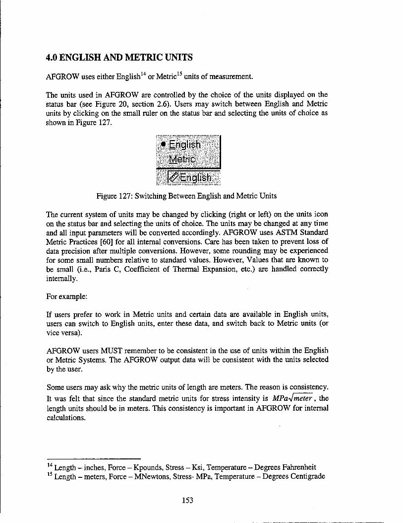
4.0 ENGLISH AND METRIC UNITS
AFGROW uses either English14 or Metric15 units of measurement.
The units used in AFGROW are controlled by the choice of the units displayed on the status bar (see Figure 20, section 2.6). Users may switch between English and Metric units by clicking on the small ruler on the status bar and selecting the units of choice as shown in Figure 127.
• English . .Metric
^English
Figure 127: Switching Between English and Metric Units
The current system of units may be changed by clicking (right or left) on the units icon on the status bar and selecting the units of choice. The units may be changed at any time and all input parameters will be converted accordingly. AFGROW uses ASTM Standard Metric Practices [60] for all internal conversions. Care has been taken to prevent loss of data precision after multiple conversions. However, some rounding may be experienced for some small numbers relative to standard values. However, Values that are known to be small (i.e., Paris C, Coefficient of Thermal Expansion, etc.) are handled correctly internally.
For example:
If users prefer to work in Metric units and certain data are available in English units, users can switch to English units, enter these data, and switch back to Metric units (or vice versa).
AFGROW users MUST remember to be consistent in the use of units within the English or Metric Systems. The AFGROW output data will be consistent with the units selected by the user.
Some users may ask why the metric units of length are meters. The reason is consistency. It was felt that since the standard metric units for stress intensity is MPa^Jmeter, the length units should be in meters. This consistency is important in AFGROW for internal calculations.
14 Length - inches, Force - Kpounds, Stress - Ksi, Temperature - Degrees Fahrenheit 15 Length - meters, Force - MNewtons, Stress- MPa, Temperature - Degrees Centigrade
153

5.0 COMPONENT OBJECT MODEL SERVER
AFGROW for Windows95/98/NT4® operates in two different modes; first, as a normal interactive Windows program, and second, as a Component Object Model (COM) Server [9]. The COM server technology is an outgrowth of the Object Linking and Embedding technology used by Microsoft for many years. A COM Server may be called from other Windows software and the results from the server can be sent back to the calling program. In the case of AFGROW, users can write Windows programs or macros to generate input data, and call AFGROW to perform structural life analyses. AFGROW can perform the life analyses and return the results directly to the calling software. The most commonly used application of this capability is seen in the following example, Figure 128, using Microsoft Excel ®.
[ \-Microsoft Excel-afqrowlxts «tic] lÖßle'Edit Slew;:lrwrt Fcrtriat:iPols BaQ:;amdow tM> :■ MlM tp:«;0f#'ß-^U-*-e.<fi>7-».?t*^^^ :|R. n|fi!*.tf| . y. fJÄrä" ' ' 'S..IIO'T.|-B /-!<s;|B*<*-fl|'s x-\~-X&\9t&\-z>--Ä>;~:&~
-liLs.^\mjs. ■-* *'-a.a ^■n-'ä-Äa|*r H ■■■■>-!
■:-:.A■.'■■■|-v-:B •■■■I •■■•••.■C--: 1 Ü -1 ' E ':-.'\ ■■ •■ :i-:.'.-.'V-iF" '■"■>- -|- G '•■■■^Ir '.:■■:■■V-i-'.-'-iH '■■<■'? V.1
2 ?<
3 4
-5:
; c:\Program Files\afgrow\dcase.sp3
SMF Model Initial A 20 1030 0.05
nitialC Output File Cycles f! 0.05 c:\Program Files\afgroW\test1.out 193461 Completed Normally
i.,8 ■.
;■:«-
.10 :'11- 12 13 14 15 16 17
22.5 1030 0.05 25 1030 0.05 30 1030 0.05 35 1030 0.05
Beta Correction Table Distance C-Direction A-DirecSon
0.001 0.99 0.99 0.2 0.95 0.98
0.05 c:\Program Files\afgrow\test2.out 124830 Completed Normally 0.05 c:\Program Files\afgroW\test3.out 81160 Completed Normally 0.05 c:\Program Files\afgrow\test4.out 36445 Completed Normally 0.05 c:\Program Files\afgroW\test5.out 15664 Completed Normally
^■Usert-onnt-' .;. ■■■.■ Ei
- - - z. Run AFGROW .
Start on Row 1 j i
Iti 19
0.4 0.9 0.95 0.6 0.875 0.95 D .
Currency Working on Row J :20 % 22
'23 524 :■ i2S':
"26: 'm i28"
2 0,87 0.95
;.,:■!'■• ..■'■ :.: 'Slop .■■■■■"-•[:'■?);'
v;
AI < I ► MI\Sh«*1 / SheeG / Shaet3 /.■... l«l am - Ready A
Figure 128: Microsoft Excel Macro Using AFGROW
The above example is a fairly simple application of the COM capabilities in AFGROW, but is intended to show how the technology may be used to perform multiple life analyses. Other uses of this capability can extend as far as a user's imagination can carry it in terms of application to structural life prediction. This capability has already been
154

used to estimate the crack growth life of specimens subjected to a corrosive environment [61].
An extensive manual on the use of AFGROW as a COM server has been released on the AFGROW Web Site [62] and will soon be available in print [63]. An excerpt from the manual is given below:
General Instructions
Before using the server version from another windows program, AFGROW MUST run at least once as a stand-alone program. When the server version is executed for the first time, Windows will recognize that it is a COM server and will look for a Type Library Binary (TLB) file (afgrow.tlb) and register AFGROW as a COM object on the local machine. Once this is complete, the AFGROW server will be available for use by other COM compatible software.
The TLB file contains detailed information that other programs use to determine which variables and sub-routines are available in AFGROW. Whenever the AFGROW server is updated and a new version is downloaded, all references to the previous server version MUST be updated.
Again, remember that the new server version will still function as the stand-alone interactive code as it has in the past. The new capability is merely an addition to AFGROW, which we hope users will find useful.
155

6.0 TUTORIAL
This section will take users through a sample problem to show how to use many of the features described in previous sections of this manual.
6.1 Problem Definition
tttttt °
4.0
ler ^
Dia. = 0.25
1.5
UHH
0.25 _±_
A
Figure 129: Sample Problem Geometry
Specimen Geometry: Dimensions: Hole Offset: Initial Crack Size: Material: Stress Spectrum:
Retardation Model: Stress State: Beta Correction: Environment:
Corner Crack at an Offset Hole in a Plate W = 4.0 in., T = 0.25 in., Dia. = 0.25 in. B = 1.5 in. c = 0.05 in., a = 0.05 in. 7050-T74 Plate (from matfile.da3) 16 Ksi to 0 Ksi 1 Cycle 12 Ksi to 8 Ksi 1000 Cycles Generalized Willenborg Model, SOR = 2.8 Automatic None N/A
156
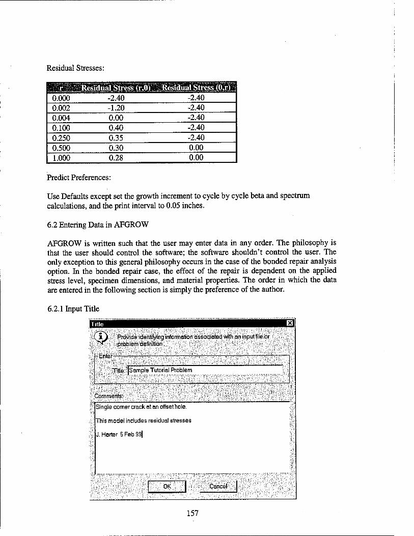
Residual Stresses:
Residual Stress (r 'ffli ISel^ÖSSesiCÖiif|!
0.000 -2.40 -2.40 0.002 -1.20 -2.40 0.004 0.00 -2.40 0.100 0.40 -2.40 0.250 0.35 -2.40 0.500 0.30 0.00 1.000 0.28 0.00
Predict Preferences:
Use Defaults except set the growth increment to cycle by cycle beta and spectrum calculations, and the print interval to 0.05 inches.
6.2 Entering Data in AFGROW
AFGROW is written such that the user may enter data in any order. The philosophy is that the user should control the software; the software shouldn't control the user. The only exception to this general philosophy occurs in the case of the bonded repair analysis option. In the bonded repair case, the effect of the repair is dependent on the applied stress level, specimen dimensions, and material properties. The order in which the data are entered in the following section is simply the preference of the author.
6.2.1 Input Title
tOG1 Provide identifying information associated with an inputfile or ^T nrahlem definition Ipäblemäefirfäon
rEntef-
TrlleSjSample Tutorial Problem
Comments:
Single corner crack at an offset hole.
This model includes residual stresses
J. Harter 5 Feb 99|
OK "Cancel
157

6.2.2 Input Material ida/dN Data
^AFGROW provides five ways of specifying material properties: fusing standard aa«^growth rate equations or tabulated data.
- Select material properly description—^-:—
, C talker Equation " :
•C Eorman Equation
■i\:-C'-NASGROEquation :;:■;:>:;
';/:■, ^<?--Harter3H^^.''V^-V-;:v'^^/^
C Tabular Lookup .'
OK;
■ Cancel
[Material Database Eil
," /XV The Harter T-Method is an adaptation of the Walker equation taken z. ^r on a poinHay-pointbasis.Jn this implementation 25 da/dN values :
The method accounts forthe stress ratio (R) shift independently at each da/dN ' .„lvalues to more accurately represent real crack growth rate data r The data are^contained in a user maintained libraryfor several materials. ':.
Browse... |c:\prögramfiles\ofgrow\i,nötfiIe.md3
|7050-T74 PLATE' - ■ ' < -_,.'■■
Available Materials:';:,;:^; ;../"■' -v. >> \:
2024 T-3 LONG CRACK DATA * 202+T851 - LONG CRACK 5- 6061-T6511 EXTRUSION
;
7075-T6511 EXTRUSION 7075-T73L-T FORGING 7075-T73L-T[DRYAIR] 707&-T73T-L FORGING Ti-6-4 ALPHA-BETA FORGING , ,s
\:V^;:.ÖK^;-V'":j "' ■■[[''■'/^■■f:-'- '.;"-;:y v' :■;:,' ' Cane -HI-'
158
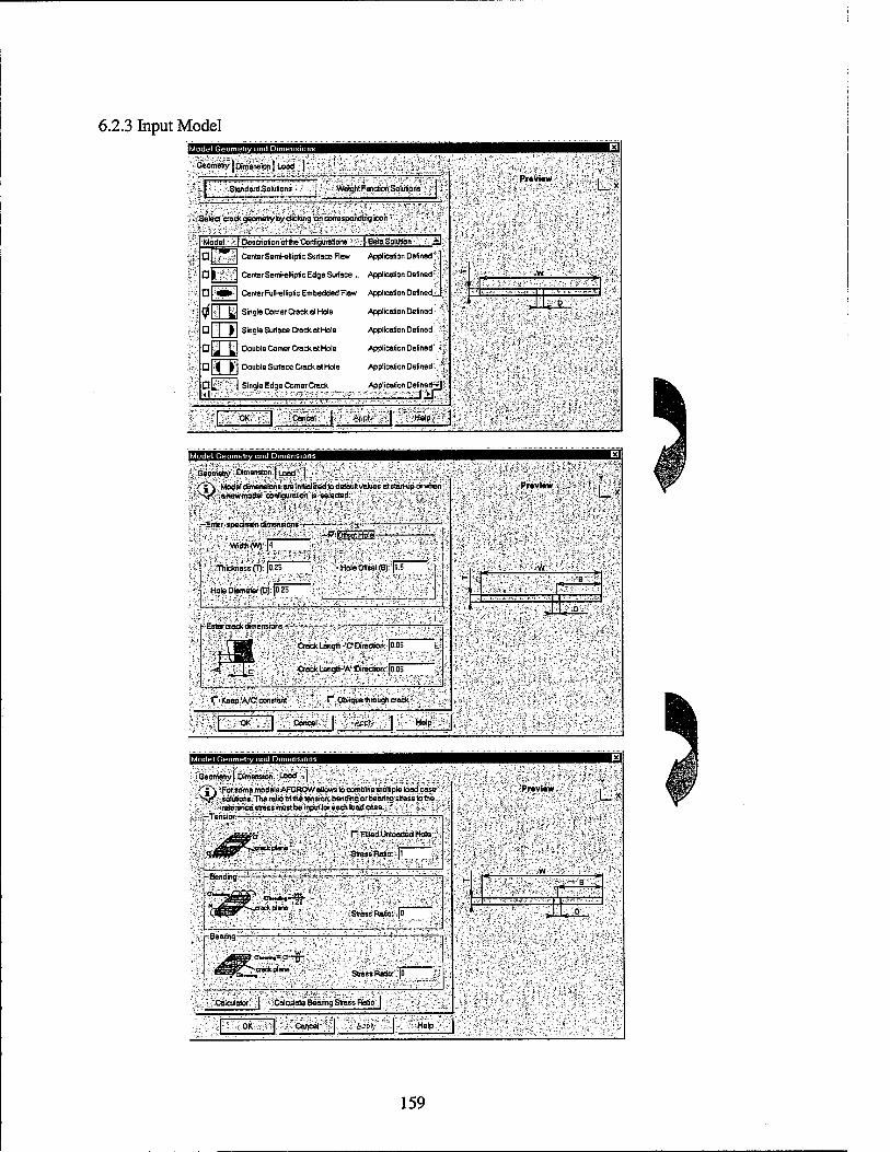
6.2.3 Input Model IM.I.III.II.I..II..UII.I.I.II..II.UI.I.H
^'GMm^lÖi^ehsion J ü)ed 1^ ;:
v.Standard-Solutions :- ■Weight FurrcSonSolirtionS';:
^Seleefc^cradkgeon^try bydiBong on correspondingicoh *
Model ■ UDe8Ciripfon6>thetor^^ h^
U \-i§!^M Center Semi-elliptic Surface Fiow Application Defined*
Op!i|Pj Center Semi-elliptic Edge Surface... Application Defined;
□ piäöh] Center Full-elliptic Embedded Raw Application Defined^
9 M JU Single Comer Crack et Hole Application Defined; '•:
Dill JH Single Surface Crack at Hole
QtJÜ Lrl Double Comer Crack at Hole
□[.l |j Double Surface Crack at Hole
D t^^'j Single Edge Comer Crack
Application Defined' ~';:
Application Defined- .^
Application Defined:-.:'!
Application Defined^': I JUT
',r-ftMy^ ;W$g
E
Pr«vi«w lit
'ß;::!0bä$& w
']J ' -r:^'~V ~J.'-!*<Y^
ti ̂SSS,f'Ä-=:!»S ^mMSM
Geometry Dimension | toed |
f^j[\ Madefdurww riiaiww-model oonfiguratiooNs selected -2
^ErtercrOÄOwerötonsT-
'■'dB» - '
.?CrackLength-'C*Direction: (0.05 - ", CrockLength-^iüiredion*JÖ^05
,l"i1Ceep:Vs/C^constoÄ,x: '^ j.^/jdblib^e.thro.ügh crock?;
± ;«iitep$ fls»ßi
(fPnvmtii ; i_*
Ö.
e * w ,i.-*B"-:.:« Iq . '
1 K«* f>;i-ft.:>'i» iH2sa
I.I.I.I.IJI^J.I..ÜI.II.I,I.I.II„I!1,UI.I,U
;■ ;Geometry|.D«nensfcm;: Load.;;j: ..-
^> ^ ^oteomemp^^^
^^Qlutions/Theratioofthe^ reference stress mustbe tnputfor each load case.
ITmsibn-' "' "" ' """ '*'" '
:::OK^^^l^v::>Ctor^-*: ^feppiy- O-tetp '•
{preivlew
Ü
- Lx
'^' .^: s-:;esw-; --■;
'* ^^^■; t.-jj-^B':
'■• .'',.-'
■■:.:■ .;,-..-;.,-,.J>i>'.T.«'"^'-^' w": ---■■- '•^~''-
*;V > *££&
159
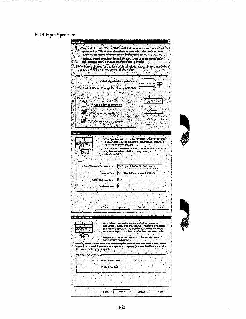
6.2.4 Input Spectram
R* sStmssMuttiplication Factor (SMF): multiplies the sfress or load levels found in spectrum SlesThis allows normalized spectra to betisecLIf actual stress'
" i •levelsarepresen^insjMctrumfiles.S^mustbesetto?, ,:; - A .
? ■', Residual Stress Strength Requirement (SPCM>$ is used for critical crack ; 'size determinationiifavatue d*er then zero is enteied.-•'., ,•; V -
SPOvK- value of stress(or load for mddelrusing load instead of stress inpuf) which ^thestmctureMUSTbeabletocariyatallchscksizes. -~'.\ -,,...' -1, ^-
iEntar-
Stress MüftiplicBfipn FactorfSMF): |1
%& ■ Residual Stress Strength Requirement (SPCM>9 trjO
:-t-
teSelectr
III T p-^r'JCreate new spectrum fjlej'j
W: P^penjipectrumfle* vS>;r;
< IffVl , r Comta^amplitudeloading^
tOK'
SCahcel"
■■:\ .The Spisctrum Wizard cre^s'SPECTRUM INFORMATION ; FILE which is required to define the load/stress htstoiytor a
. given crock growth analysts. . ; Spectra may broken into several sub-spec*» andsub-spectra may be grouped and divided among a number of ~ sub-spectrum ties. " ■■.'".
r Enter—TT.—:- -..' .. -... ...,—^... ':■■'■ ■'.":. -''■..■'■'■'■ '■•.'■■ - ■■.,-' ■ ■' 1
]",- Base Filename (no exlention): 1: '■:.' .•:.'.■ "■■..;'■ ■■■
|CAProgram Files\AFGROW\sample
1. , Spectrum Title: lAFGROWTutorial Sample Spectrum
1 . .*': Label forSub-spectrum: |Block
1, ' . . . , Number ol files:
\ : ■':.■ ' '■'■■■■■■■
M:.J,M^ -yM^^^'
N.ext> Cancel Help
Type ot spectrum
Acydebycyde spectrum is one Inwhich each max-min" tood/stressisappliedfororwpjcyde.Thismoybethoughtof
. . V fts a realtime spectrum.The blocked spectrum is one where'. each max-min pair is applied far some finite number of cycles.
; , .Mahytimes.8peära8iepresentedinthisfomiattosave :~. /■; ■:;.,.:;■;;- ;v,:-.; ';...'■ "computer time and space. :
: ''l\^'':.\-.:
lnmanycases.theuseottheblockedtorm8tproduc8sverylp«e difference in terms of the ':'analysis. In general the more times a spectrum is repeated, the less the difference in using blocked or cyde-by-cyde spectra. . ;
-SelectType of Spectrum-
g [Blocked Cydesj
C CydebyCyde
«Back N.ext> Cancel Help
160

Number of Sub-spectra
ssub-spectrathat can make up« spectrum. Tlie limits are 10 sub-spectra per file.
SÄf-|I§täK -. ' A f rN
Number of Sub-«pee*a: |1 £ \
T*llmporl from file! i „
• • Browse
^ , ;^; *:•■?§"''■?*''$■•&
<fiack | Mexl> | ' Cancel | Help |
Number of Stress levels
Ttefe-araJtmits ,& maratat mode/placed oa*e nurnoet of stressJävBtsihatiÄnmafetiiiatspeäram.'ITielimits ore2S'* levels pei.spectnjni. ■'
file»! Sab-spectrum *1
-t n»rr^mracoiJsii3ess;iBveisssv?w^wS=s^? ̂ iri'-W»Vv;t^TK*.f*-T''.'^.",«" ^'W*?J^X'7X^VZ----:"^V't'~-y '
Number of Stress levels- ,
'?'.-" 1:.... ä.
"'*'*. * D;l ^•~ ^iHSl^lliv^l •»'errjÄ^e* ' j. -
* J - g '
r. 'S V=ffi*:&?&: &;' 'it' ;'? %~" 1 ^ * ^ili^V /* S: 7S «£:?' vi&'&VsK ~?*?*.^-':/-''^-??T:*Z'CW''.
Vj^-^-jp'^^ . „ *"*■"• . '
SfiW*'; WßÜS'l fCahee|;; ■Help
FrnffHBHi File #1 Sub-spectrum #1
Onp'rtSpecWWStress/llbäa ße^lsÄormäSqninthe' .following format • ■
;EritarStress.bevels-
: fW'iW :1000
Set ■ '¥.-■ Max Mm Cycles
l 16.000000 0.000000 1 1 2 12.000000 8.000000 1000
<;gack. Cjext> | Cancel. fleip:
161
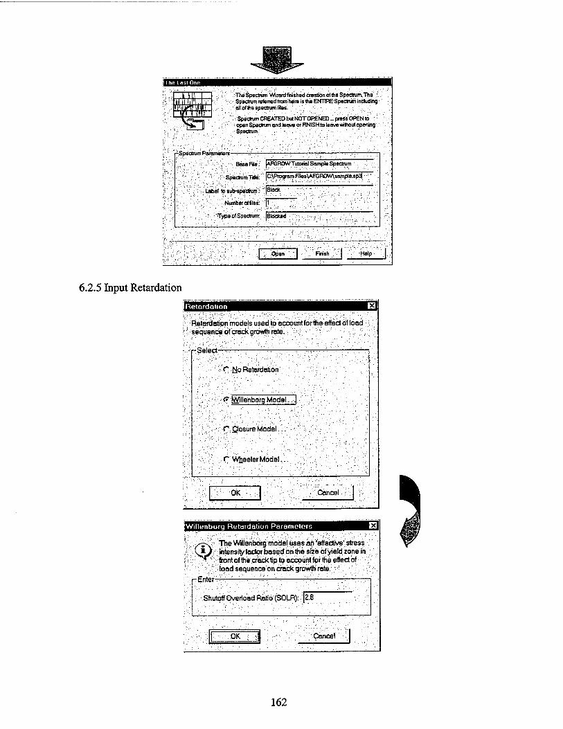
':■ The Spectrum Wizard finished creation of the Spectrum. The ;. Spectrum referred from here is the ENTIRE Spectrum including nilo(the spectrum Hies. '".*; :.
Spectrum CREATED but NOTOPENED ^ press OPEN to open Spectrum and leave or FINISH to leave without opening
: Spectrum. '.''v-'
-Spectrum Parameter» .
'.,:',;, -;.:' '■:■'".:■•:';- Base File:
Spectrum Trte:
label fo su'b-spedrum:
Number of files:
TypeofSpedrum:
- ■' ' ■:: ... ■-..■.'
pVFGROWTutoriol Sample Spectrum '
|a\ProgramFilesW:GROW\sample.sp3j
|8lock -
\\ - (Blocked
.Open Finish ; Help
6.2.5 Input Retardation
Retardation
Retardation models used to accountforthe effect of load jsequence of crack growth rate. " *
:Select-
C Mo Rstardarjon
(?fefVillenborg Model..}
C Closure Model...
,r Wheeler Model,!
OK Cancel
Willenborq Retardation Parameters
>srO'' The Willenborg model uses ah 'effective' stress SjO" intensKy factor basedon the size of yield zone in ^^ ■• front of the crack tip to account forthe effect of
load sequence on crack growth rate. '
rEnter— -^—- ^— : —
Shutoff Overload Ratio (SOLR): 2.8
OK -■-■'■■] : ■.:■■ "Cancel
162

6.2.6 Stress State
Stress State
M |The Stress State Data provide a means of approximating the actual value of yield zone size and fracture toughness in each crack growth direction.
nSelect-
•*<? Determine Stress State automatically
C EnterStress State manually
ßOJtGl
Cancel
6.2.7 Residual Stresses Residual Stresses
® SäFGROW offers the optiorr to model the effect of residual stresses on crack growth by reading in a table of residual stresses as a function'of
. crack length.than AFGROW uses these values to generates a table of 'ResidualStress IntensityFectors'^SIF).-
S(xy)-value of astress in Z axis directioa' " r-distancefromthecenterpointofthecrackalong XorYaxis;
: Select type of Datar
P Stress jr.: Residual K*
•Enter"Stress;arirj V-Üse up to ;25jsets-
Numberof Sets: - |7 jr|
:Set;fi® r : vSEöJ':: 'S(0;r) :, H 1 0 0.02
-2.4 ■ -1.2
-2.4 \!Z^M: -2.4 SC-
•3 0.04 0 -2.4 4 0.1 ! 0.4 -2.4
.,'"5 ..4~- 0.25 : 0.35 -2.4 6 0.5 i 0.3 0 d
W&f. iGanceli
-Generate SIF table using-
P Gauss Integration
C'Weiqht Function
163

6.2.8 Predict Preferences
Predict Function Preferences
growth increment [fiu^lnteivais| ÖutoüVObJjoftsj Proi < 1 '>■.
/"•V AFGRCW uses the Vroman Integration technique \jy' when a blocked spectrum is input To minimize an •^T' error in predicted crack propagation times it is not
recomended for Max Growth Increment value to
m Cycle by cycle calculation can significantly increase a calculation time.
■Select-
JP" Cycle by''^de^pedn^.caj.culaöon^.'' - ■■-.■'
15/ [Cycle by Cycle Beta and Spectrum calculation I
OK Cancel Save Default
Predict Function Preferences
Growth Increment Putput Intervals j Output Options] Proi* I'>'
Print Output Data at—'.:",■ -—.'.■....•- - .,' ;...■...; :,.' .
.,<? Specified Dack Growth Increment
"■C". Specified Spectrum Cyclic Increment
C After each Spectrum Stress Level
Dack Growth |0.05_
V^Display Lifetime in Hours
OK j Cancel Save Default
164
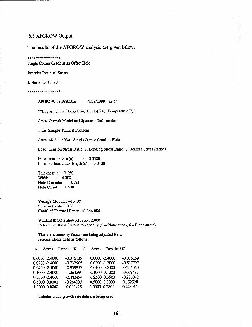
6.3 AFGROW Output
The results of the AFGROW analysis are given below.
Single Corner Crack at an Offset Hole
Includes Residual Stress
J. Harter 23 Jul 99
AFGROW v3.983.10.6: 7/23/1999 15:44
**English Units [ Length(in), Stress(Ksi), Temperature(F) ]
Crack Growth Model and Spectrum Information
Title: Sample Tutorial Problem
Crack Model: 1030 - Single Corner Crack at Hole
Load: Tension Stress Ratio: 1, Bending Stress Ratio: 0, Bearing Stress Ratio: 0
Initial crack depth (a) : 0.0500 Initial surface crack length (c): 0.0500
Thickness : 0.250 Width : 4.000 Hole Diameter: 0.250 Hole Offset: 1.500
Young's Modulus =10400 Poisson's Ratio =0.33 Coeff. of Thermal Expan. =1.34e-005
WILLENBORG shut-off ratio : 2.800 Determine Stress State automatically (2 = Plane stress, 6 = Plane strain)
The stress intensity factors are being adjusted for a residual stress field as follows:
Stress Residual K C Stress Residual K
0.0000 -2.4000 -0.076139 0.0000 -2.4000 -0.076169 0.0200 -2.4000 -0.732505 0.0200-1.2000 -0.517797 0.0400 -2.4000 -0.939953 0.0400 0.0000 -0.254020 0.1000-2.4000 -1.364590 0.1000 0.4000 -0.059487 0.2500 -2.4000 -2.482494 0.2500 0.3500 -0.226042 0.5000 0.0000 -0.264293 0.5000 0.3000 0.132328 1.0000 0.0000 0.002428 1.0000 0.2800 0.428985
Tabular crack growth rate data are being used
165
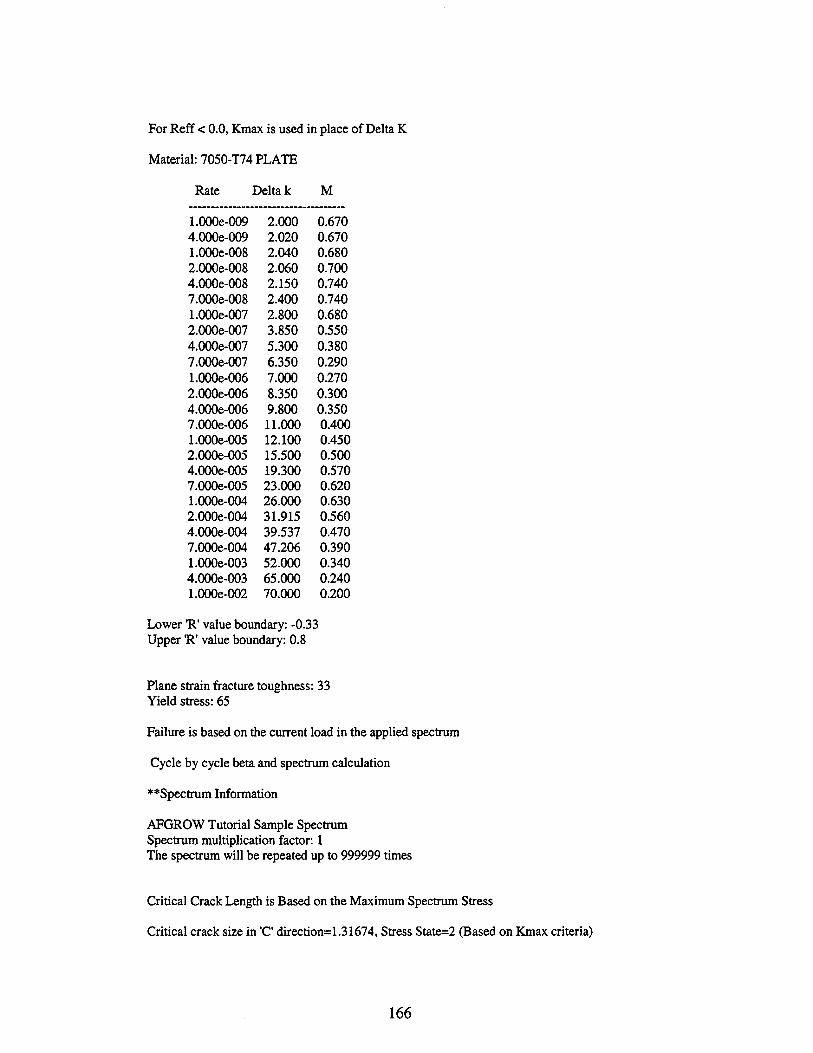
For Reff < 0.0, Kmax is used in place of Delta K
Material: 7050-T74 PLATE
Rate Delta k M
1.000e-009 2.000 0.670 4.000e-009 2.020 0.670 1.000e-008 2.040 0.680 2.000e-008 2.060 0.700 4.000e-008 2.150 0.740 7.000e-008 2.400 0.740 1.000e-007 2.800 0.680 2.000e-007 3.850 0.550 4.000e-007 5.300 0.380 7.000e-007 6.350 0.290 1.000e-006 7.000 0.270 2.000e-006 8.350 0.300 4.000e-006 9.800 0.350 7.000e-006 11.000 0.400 1.000e-005 12.100 0.450 2.000e-005 15.500 0.500 4.000e-005 19.300 0.570 7.000e-005 23.000 0.620 1.000e-004 26.000 0.630 2.000e-004 31.915 0.560 4.000e-004 39.537 0.470 7.000e-004 47.206 0.390 1.000e-003 52.000 0.340 4.000e-003 65.000 0.240 1.000e-002 70.000 0.200
Lower "R' value boundary: -0.33 Upper "R' value boundary: 0.8
Plane strain fracture toughness: 33 Yield stress: 65
Failure is based on the current load in the applied spectrum
Cycle by cycle beta and spectrum calculation
**Spectrum Information
AFGROW Tutorial Sample Spectrum Spectrum multiplication factor: 1 The spectrum will be repeated up to 999999 times
Critical Crack Length is Based on the Maximum Spectrum Stress
Critical crack size in 'C direction= 1.31674, Stress State=2 (Based on Kmax criteria)
166
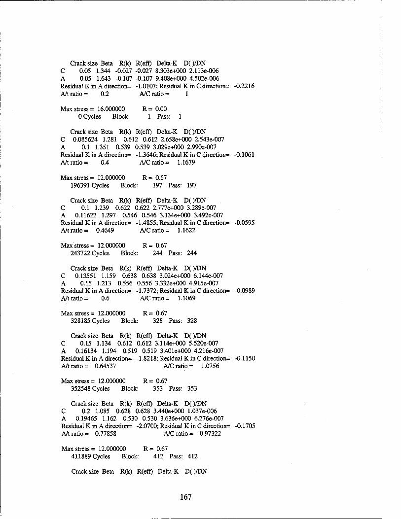
Crack size Beta R(k) R(eff) Delta-K D( )/DN C 0.05 1.344 -0.027 -0.027 8.303e+000 2.113e-006 A 0.05 1.643 -0.107 -0.107 9.408e+000 4.502e-006 Residual K in A directions -1.0107; Residual K in Cdirection= -0.2216 A/t ratio = 0.2 A/C ratio = 1
Max stress = 16.000000 R = 0.00 0 Cycles Block: 1 Pass: 1
Crack size Beta R(k) R(eff) Delta-K D( )/DN C 0.085624 1.281 0.612 0.612 2.658e+000 2.543e-007 A 0.1 1.351 0.539 0.539 3.029e+000 2.990e-007 Residual K in A direction= -1.3646; Residual K in C directions -0.1061 A/t ratio = 0.4 A/C ratio = 1.1679
Max stress = 12.000000 R= 0.67 196391 Cycles Block: 197 Pass: 197
Crack size Beta R(k) R(eff) Delta-K D( )/DN C 0.1 1.239 0.622 0.622 2.777e+000 3.289e-007 A 0.11622 1.297 0.546 0.546 3.134e+000 3.492e-007 Residual K in A directions -1.4855; Residual Kin Cdirection= -0.0595 A/t ratio = 0.4649 A/C ratio = 1.1622
Max stress = 12.000000 R= 0.67 243722 Cycles Block: 244 Pass: 244
Crack size Beta R(k) R(eff) Delta-K D( )/DN C 0.13551 1.159 0.638 0.638 3.024e+000 6.144e-007 A 0.15 1.213 0.556 0.556 3.332e+000 4.915e-007 Residual K in A directions -1.7372; Residual K in C directions -0.0989 A/t ratio= 0.6 A/C ratios 1.1069
Max stress = 12.000000 R= 0.67 328185 Cycles Block: 328 Pass: 328
Crack size Beta R(k) R(eff) Delta-K D( )/DN C 0.15 1.134 0.612 0.612 3.114e+000 5.520e-007 A 0.16134 1.194 0.519 0.519 3.401e+O0O 4.216e-007 Residual K in A directions -1.8218; Residual K in C directions -0.1150 A/t ratios 0.64537 A/C ratios 1.0756
Max stress = 12.000000 R = 0.67 352548 Cycles Block: 353 Pass: 353
Crack size Beta R(k) R(eff) Delta-K D( )/DN C 0.2 1.085 0.628 0.628 3.440e+000 1.037e-006 A 0.19465 1.162 0.530 0.530 3.636e+000 6.276e-007 Residual K in A directions -2.0700; Residual K in C directions -0.1705 A/t ratios 0.77858 A/C ratio = 0.97322
Max stress = 12.000000 R= 0.67 411889 Cycles Block: 412 Pass: 412
Crack size Beta R(k) R(eff) Delta-K D( )/DN
167
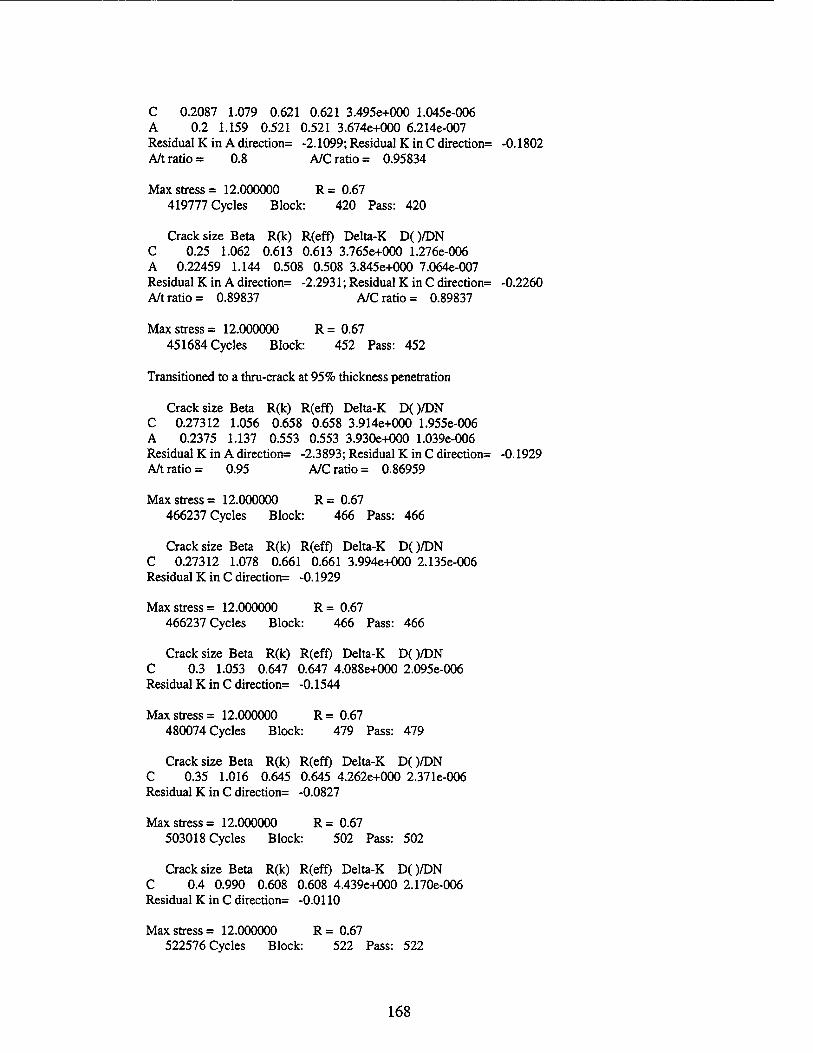
C 0.2087 1.079 0.621 0.621 3.495e+000 1.045e-006 A 0.2 1.159 0.521 0.521 3.674e+000 6.214e-007 Residual K in A direction -2.1099; Residual K in Cdirection= -0.1802 A/t ratio = 0.8 A/C ratio = 0.95834
Max stress = 12.000000 R = 0.67 419777 Cycles Block: 420 Pass: 420
Crack size Beta R(k) R(eff) Delta-K DQ/DN C 0.25 1.062 0.613 0.613 3.765e+000 1.276e-006 A 0.22459 1.144 0.508 0.508 3.845e+000 7.064e-007 Residual K in A direction= -2.2931; Residual K in C direction= -0.2260 A/t ratio = 0.89837 A/C ratio = 0.89837
Max stress = 12.000000 R = 0.67 451684 Cycles Block: 452 Pass: 452
Transitioned to a thru-crack at 95% thickness penetration
Crack size Beta R(k) R(eff) Delta-K DQ/DN C 0.27312 1.056 0.658 0.658 3.914e+000 1.955e-006 A 0.2375 1.137 0.553 0.553 3.930e+000 1.039e-006 Residual K in A direction= -2.3893; Residual K in C direction= -0.1929 A/t ratio = 0.95 A/C ratio = 0.86959
Max stress = 12.000000 R = 0.67 466237 Cycles Block: 466 Pass: 466
Crack size Beta R(k) R(eff) Delta-K DQ/DN C 0.27312 1.078 0.661 0.661 3.994e+000 2.135e-006 Residual K in C direction= -0.1929
Max stress = 12.000000 R= 0.67 466237 Cycles Block: 466 Pass: 466
Crack size Beta R(k) R(eff) Delta-K DQ/DN C 0.3 1.053 0.647 0.647 4.088e+000 2.095e-006 Residual K in C direction= -0.1544
Max stress = 12.000000 R= 0.67 480074 Cycles Block: 479 Pass: 479
Crack size Beta R(k) R(eff) Delta-K D( )/DN C 0.35 1.016 0.645 0.645 4.262e+000 2.371e-006 Residual K in C direction= -0.0827
Max stress = 12.000000 R= 0.67 503018 Cycles Block: 502 Pass: 502
Crack size Beta R(k) R(eff) Delta-K DQ/DN C 0.4 0.990 0.608 0.608 4.439e+000 2.170e-006 Residual K in C direction= -0.0110
Max stress = 12.000000 R= 0.67 522576 Cycles Block: 522 Pass: 522
168
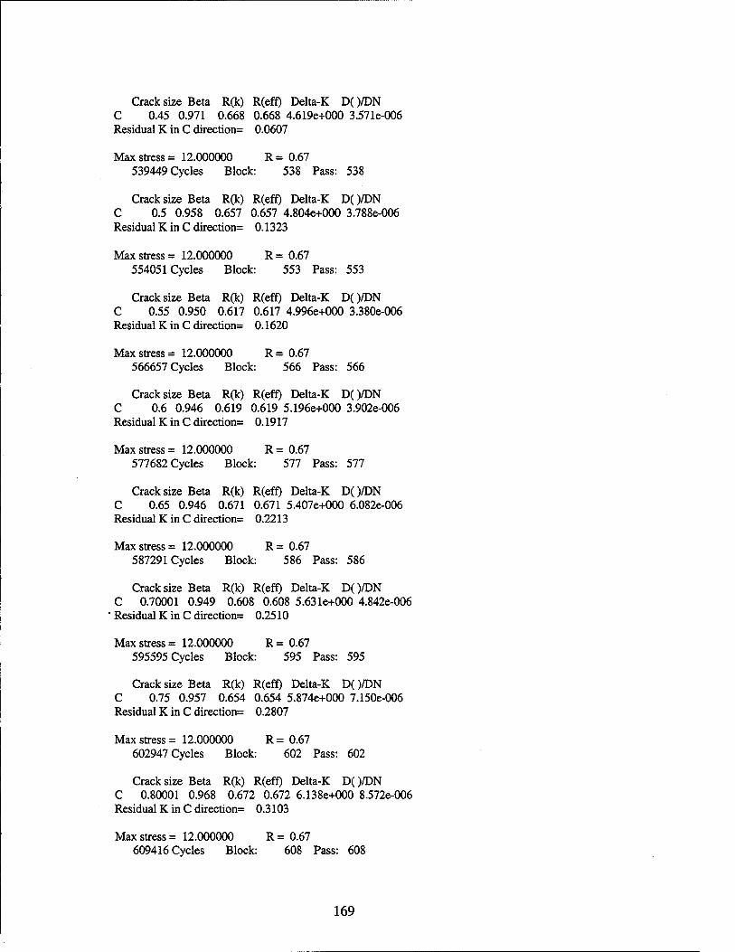
Crack size Beta R(k) R(eff) Delta-K D( )/DN C 0.45 0.971 0.668 0.668 4.619e+000 3.571e-006 Residual K in C direction= 0.0607
Max stress = 12.000000 R = 0.67 539449 Cycles Block: 538 Pass: 538
Crack size Beta R(k) R(eff) Delta-K D( )/DN C 0.5 0.958 0.657 0.657 4.804e+000 3.788e-006 Residual K in C direction= 0.1323
Max stress = 12.000000 R = 0.67 554051 Cycles Block: 553 Pass: 553
Crack size Beta R(k) R(eff) Delta-K D()/DN C 0.55 0.950 0.617 0.617 4.996e+000 3.380e-006 Residual K in C direction= 0.1620
Max stress = 12.000000 R= 0.67 566657 Cycles Block: 566 Pass: 566
Crack size Beta R(k) R(efr) Delta-K D( )/DN C 0.6 0.946 0.619 0.619 5.196e+000 3.902e-006 Residual K in C direction= 0.1917
Max stress = 12.000000 R= 0.67 577682 Cycles Block: 577 Pass: 577
Crack size Beta R(k) R(eff) Delta-K DQ/DN C 0.65 0.946 0.671 0.671 5.407e+000 6.082e-006 Residual K in C direction= 0.2213
Max stress = 12.000000 R= 0.67 587291 Cycles Block: 586 Pass: 586
Crack size Beta R(k) R(eff) Delta-K D()/DN C 0.70001 0.949 0.608 0.608 5.631e+000 4.842e-006 Residual K in C direction= 0.2510
Max stress = 12.000000 R = 0.67 595595 Cycles Block: 595 Pass: 595
Crack size Beta R(k) R(eff) Delta-K D( )/DN C 0.75 0.957 0.654 0.654 5.874e+000 7.150e-006 Residual K in C direction= 0.2807
Max stress = 12.000000 R = 0.67 602947 Cycles Block: 602 Pass: 602
Crack size Beta R(k) R(eff) Delta-K D( )/DN C 0.80001 0.968 0.672 0.672 6.138e+000 8.572e-006 Residual K in C direction= 0.3103
Max stress = 12.000000 R = 0.67 609416 Cycles Block: 608 Pass: 608
169

Crack size Beta R(k) R(eff) Delta-K D( )/DN C 0.85001 0.984 0.672 0.672 6.431e+000 9.579e-006 Residual K in C direction 0.3400
Max stress = 12.000000 R = 0.67 615213 Cycles Block: 614 Pass: 614
Crack size Beta R(k) R(eff) Delta-K D( )/DN C 0.90001 1.005 0.673 0.673 6.761e+000 1.076e-005 Residual K in C direction= 0.3697
Max stress = 12.000000 R= 0.67 620358 Cycles Block: 619 Pass: 619
Crack size Beta R(k) R(eff) Delta-K D( )/DN C 0.95001 1.033 0.651 0.651 7.138e+000 1.124e-005 Residual K in C direction= 0.3993
Max stress = 12.000000 R= 0.67 624925 Cycles Block: 624 Pass: 624
Crack size Beta R(k) R(eft) Delta-K DQ/DN C 1 1.069 0.648 0.648 7.579e+000 1.280e-005 Residual K in C direction= 0.4290
Max stress = 12.000000 R= 0.67 628913 Cycles Block: 628 Pass: 628
Crack size Beta R(k) R(eff) Delta-K D( )/DN C 1.05 1.116 0.672 0.672 8.109e+000 1.629e-005 Residual K in C direction= 0.4290
Max stress = 12.000000 R = 0.67 632353 Cycles Block: 631 Pass: 631
Crack size Beta R(k) R(eff) Delta-K D( )/DN C 1.1 1.178 0.672 0.672 8.763e+000 1.942e-005 Residual K in C direction= 0.4290
Max stress = 12.000000 R = 0.67 635282 Cycles Block: 634 Pass: 634
Crack size Beta R(k) R(eff) Delta-K D( )/DN C 1.15 1.263 0.609 0.609 9.606e+000 1.960e-005 Residual K in C direction= 0.4290
Max stress = 12.000000 R = 0.67 637671 Cycles Block: 637 Pass: 637
Crack size Beta R(k) R(eff) Delta-K D( )/DN C 1.2 1.385 0.671 0.671 1.076e+001 3.121e-005 Residual K in C direction= 0.4290
Max stress = 12.000000 R= 0.67 639587 Cycles Block: 638 Pass: 638
170

Crack size Beta R(k) R(eff) Delta-K D( )/DN C 1.25 1.576 0.655 0.655 1.249e+001 4.231e-005 Residual K in C direction 0.4290
Max stress = 12.000000 R= 0.67 641009 Cycles Block: 640 Pass: 640
Crack size Beta R(k) R(eff) Delta-K D()/DN C 1.3001 1.931 0.645 0.645 1.561e+001 7.107e-005 Residual K in C direction= 0.4290
Max stress = 12.000000 R= 0.67 641907 Cycles Block: 641 Pass: 641
*********Fracture based on' Kmax' Criteria (current maximum stress)
Crack size Beta R(k) R(eff) Delta-K DQ/DN C 1.3456 2.830 0.669 0.669 2.327e+001 5.675e-004 Residual K in C direction= 0.4290
Max stress = 12.000000 R= 0.67 642253 Cycles Block: 641 Pass: 641
Stress State in 'C direction (PSC): 2
Fracture has occurred - run time : 0 hour(s) 0 minute(s) 37 second(s)
171

REFERENCES
1. Harter, James A., "MODGRO Users manual, Version 1.2, Technical Memorandum," AFWAL-TM-88-157-FIBE, AFWAL Flight Dynamics Laboratory, Wright-Patterson AFB, OH, 1988
2. Elber, Wolf, "The Significance of Fatigue Crack Closure," Damage Tolerance in Aircraft Structures, ASTM STP 486, American Society for Testing and Materials, 1971, pp. 230-242
3. Creager, Matthew, Personal Conversations with James A. Harter, Northrop Corporation, Pico Rivera, CA, 1982-1983
4. Sunder, R, Personal Conversations with James A. Harter, U.S. Air Force Materials Directorate, Wright-Patterson, AFB, OH, 1988-1989
5. Kaplan, M, Personal Conversations with James A. Harter, Willis and Kaplan, 1988- 1989
6. Krishnan, S., Boyd, K.L., and Harter, J.A., "Structural Integrity Analysis and Verification of Aircraft Structures - AFGROW User's Manual: Version 3.1.1," WL- TR-97-3053, Wright Laboratory Flight Dynamics Directorate, Wright-Patterson AFB, OH, 1997
7. Boyd, K., Krishnan, S., Litvinov, A., Eisner, J., Harter, J., Ratwani, M., and Glinka, G., "Development of Structural Integrity Analysis Technologies for Aging Aircraft Structures: Bonded Composite Patch Repair & Weight Function Methods," WL-TR- 97-3105, Wright Laboratory Flight Dynamics Directorate, Wright-Patterson AFB, OH, 1997
8. Tuegel, E., Strain-Life Crack Initiation Life Software, Provided by Analytical Processes and Engineered Solutions (AP/ES), Inc., 1996
9. Brockschmidt, Kraig, "Inside OLE," 2nd Edition, Microsoft Press, 1995
10. Heath, B.J., and Grandt, A.F., "Stress Intensity Factors for Coalescing and Single Corner Flaws Along a Hole Bore in a Plate," Engineering. Fracture Mechanics, Vol 19, pp. 665-673,1984
11. Kamei, A., and Yokobori, T., "Some Results on Stress Intensity Factors of the Cracks and/or Slip Bands System," Reports of The Research Institute for Strength and Fracture of Materials, Special Issue, Tohoku University, Sendai, Japan, December 1974
172
12. Walker, K., 'The Effect of Stress Ratio During Crack Propagation and Fatigue for 2024-T3 and 7075-T6 Aluminum," ASTM STP 462, American Society for Testing and Materials, 1970
13. Forman, R.G., Hearney, V.E., and Engle, R.M., "Numerical Analysis of Crack Propagation in Cyclic-Loaded Structures," Journal of Basic Engineering, Trans of ASME, Vol. 89,1967
14. Forman, R.G., and Mettu, S.R., "Behavior of Surface and Corner Cracks Subjected to Tensile and Bending Loads in Ti-6A1-4V Alloy," Fracture Mechanics 22nd
Symposium, Vol. 1, ASTM STP 1131, H.A. Ernst, A. Saxena and D.L. McDowell, eds., American Society for Testing and Materials, Philadelphia, 1992
15. Harter, James A., "MODGRO Users manual, Version 1.2, Technical Memorandum," AFWAL-TM-88-157-FJJBE, AFWAL Flight Dynamics Laboratory, Wright-Patterson AFB, OH, Revised in July 1994
16. Newman, J.C., and Raju, IS., "Stress Intensity Factor Equations for Cracks in Three- Dimensional Bodies Subjected to Tension and Bending Loads," Chapter 9, Computational Methods in the Mechanics of Fracture, Elsvier Science Publishers B.V., 1986
17. Zhao, W., J. C. Newman, Jr., M. A. Sutton, X. R. Wu, and K. N. Shivakumar, "Analysis of Corner Cracks at Hole by a 3-D Weight Function Method with Stresses from Finite Element Method," NASA Technical Memorandum 110144, July 1995
18. Zhao, W. and Newman, Jr., J. C, Electronic Communication, Unpublished NASA Langley Research Center Results, 24 February 1998
19. Hall, L.H. et al., "Fracture and Fatigue of Surface Flaws and Flaws Originating at Fastener Holes," Volume 1, AFFDL-TR-74-47,1973
20. Harter, James A., "An Alternative Closed-Form Stress Intensity Solution for Single Part-Through and Through-rhe-Thickness Cracks at Offset Holes," AFRL-VA-WP-TR-1999-3001,1999
21. Ball, D.L., "The Development of Mode I, Linear-Elastic Stress Intensity Factor Solutions for Typical Structural Details," MR(FF)-1006, Lockheed Martin Tactical Aircraft Systems, 31 Dec 1996
22. Harter, James A., Empirical Fit to Finite Element Results Generated at WPAFB, OH by Mr. Deviprasad Taluk (Eagle Aeronautics, Inc.), July 1999
23. Newman, J.C., Jr., "Fracture Mechanics Parameters for Small Fatigue Cracks, " Small-Crack Test Methods, ASTM STP 1149, J. Larsen and J.E. Allison, Eds., American Society for Testing and Materials, Philadelphia, 1992, pp. 6-33
173
24. Shivakumar, V., and Hsu, Y.C., "Stress Intensity Factors for Cracks Emanating from the Loaded Fastener Hole," Presented at the International Conference on Fracture Mechanics and Technology, Hong Kong, March 1977
25. Zatz, I.J., Eidenoff, H.L., and Armen, H. Jr., "An Application of the Energy Release Rate Concept to Crack Growth in Attachment Lugs," AJAA Paper No. 81-0491
26. Raju, I.S., and Newman, J.C., "Stress Intensity Factors Circumferential Surface Cracks in Pipes and Rods," Presented at the Seventeenth National Symposium on Fracture Mechanics, Albany, NY, 1984
27. Tada, H., Paris, P.C., and Irwin, G.R., "The Stress Analysis of Cracks Handbook," Second Edition, p. 2.2, Paris Productions, Inc., St Louis, MO, 1985
28. Yuuki, R. and Ejima, K., Stress Intensity Evaluation for Surface Cracks by Means of Boundary Element Method and Influence Function Method and the Surface Crack Extension Analysis, Trans. Japan Soc. Mech. Engrs., Vol. 56, No. 524 (1990), pp. 791-797
29. Isida, M., "Method of Laurent Series Expansion for Internal Crack Problems," Ch. 2 in Mechanics of Fracturel, Methods of Analysis and Solutions of Crack Problems, G.C. Sih, ed., Noordhoff International, 1973
30. Kathiresan, K., Hsu, T.M. and Brussat, T.R., "Advanced Life Analysis Methods - Crack Growth Analysis Methods for Attachment Lugs," AFWAL-TR-84-3080 Vol. 2, Air Force Flight Dynamics Laboratory, Wright-Patterson AFB OH, September 1984
31. Empirical fit to Reference [22], and unpublished Boundary integral analysis at NASA/Langley Research Center, Hampton, VA
32. Roberts, R., and Rich, T., Stress Intensity Factors for Plate Bending, Trans. ASME, Journal of Applied Mechanics, Vol. 34, No. 3, September 1967, pp. 777-779
33. Isida, M., "Effects of Width and Length on Stress Intensity Factors of Internally Cracked Plates Under Various Boundary Conditions," International Journal of Fracture Mechanics, Vol 7, No. 3,1971
34. Fawaz, S.A., "Application of the Virtual Crack Closure Technique to Calculate Stress Intensity Factors for Through Cracks with an Elliptical Crack Front," Engineering Fracture Mechanics, 59 (1998), pp. 327-342
35. Fawaz, S.A., "Stress Intensity Factor Solutions for Part-Elliptical Through Cracks," accepted for publication in Engineering Fracture Mechanics, 1998
174

36. Tada, H., Paris, P.C., and Irwin, G.R., "The Stress Analysis of Cracks Handbook," Second Edition, p. 19.1, Paris Productions, Inc., St Louis, MO, 1985
37. Tada, H., Paris, P.C., and Irwin, G.R., "The Stress Analysis of Cracks Handbook," Second Edition, p. 2.11, Paris Productions, Inc., St Louis, MO, 1985
38. http://www.mne.ksu.edu/~franc2d/
39. Tada, H, Paris, P.C., and Irwin, G.R., "The Stress Analysis of Cracks Handbook," Second Edition, p. 2.7, Paris Productions, Inc., St Louis, MO, 1985
40. Saxena, A. and Hudak, S.J., Jr., "Review and Extension of Compliance Information for Common Crack Growth Specimens," International Journal of Fracture, Vol. 14, No. 5, Sijthoff & Noordhoff International Publishers, The Netherlands, 1978
41.Forman, R.G., and Shivakumar, V., "Growth Behaviour of Surface Cracks in the Circumferencial Plane of Solid and Hollow Cylinders," Presented at the Seventeeth National Symposium on Fracture Mechanics, Albany, NY, 1984
42.Forman, R.G., Hickman, J.C., and Shivakumar, V., "Stress Intensity Factors for Circumferencial Through Cracks in Hollow Cylinders Subjected to Combined Tension and Bending Loads," Engineering Fracture Mechanics
43. Gallagher, J.P., "A Generalized Development of Yield-Zone Models," AFFDL-TM- 74-28, Air Force Flight Dynamics Laboratory, Wright-Patterson Air Force Base, Ohio, 1974
44. Chang, J.B., and Cheng, J.S., "Cost-Effective Fatigue Crack Growth Analysis for Flight Spectrum Loading," NA-78-629, Rockwell International, North American Aircraft Division, Los Angeles, 1978
45. Newman, J.C., "A Crack Closure Model for Predicting Fatigue Crack Growth Under Aircraft Spectrum Loading," NASA TM-81941,1981
46. Sadananda, K., and Vasudevan, A.K., "Short Crack Growth and Internal Stresses," Int. Journal of Fatigue, Vol. 19, pp. 99-109,1997
47. Lang, M. and Marci, G, "Reflecting on the Mechanical Driving Force for Fatigue Crack Propagation," Fatigue and Fracture Mechanics, Vol. 29, Eds. T.L. Panontin and S.D. Sheppard, ASTM-STP 1332,1997 (In Press)
48. Walker, Kevin, Personal Conversations and Correspondence with James A. Harter, Australian Defense Department, Defense Science and Technology Organization (DSTO), 1997-98
175

49. Wheeler, O.E., "Spectrum Loading and Crack Growth," Transaction of the ASME, Journal of Basic Engineering, pp. 181-186, March 1972
50. Harter, James A., "Experimental Determination of Stress State for Common Aircraft Alloys," to be published as an Air Force technical report, 1999
51. Broek, D., "Elementary Fracture Mechanics," Third Edition, Nijhoff, 1983
52. Standard Test Method for Plane-Strain Fracture Toughness of Metallic Materials, E 399 - 90, Annual Book of ASTM Standards, American Society for Testing and Materials, ASTM Committee E-8,1993
53. Perez, R., Tritsch, D.E., and Grandt, A.F., Jr., "Interpolative Estimates of Stress Intensity Factors for Fatigue Crack Growth Predictions," Engineering Fracture Mechanics, Vol. 24, No. 4, pp. 629-633,1986
54. Tada, H., Paris, P.C., and Irwin, G.R., "The Stress Analysis of Cracks Handbook," Second Edition, p. 3.6, Paris Productions, Inc., St Louis, MO, 1985
55. Perez, R. "Aging Aircraft Structures Database," AFRL-VA-WP-TR-1998-3022, March, 1998
56. Neuber, H., "Theory of Stress Concentration for Shear-Strained Prismatical Bodies with Arbitrary Nonlinear Stress-Strain Law," Trans. ASME, Journal of Applied Mechanics, pp. 544-550, Dec 1960
57. Smith, K.N., Watson, P., and Topper, T.H., "A Stress-Strain Function for the Fatigue of Metals," Journal of Materials, Vol. 5, No. 4, pp. 767-778,1970
58. Peterson, R.E., "Stress Concentration Factors," John Wiley and Sons, 1974
59. Mitchell, M.R., "Fundamentals of Modern Fatigue Analysis for Design," ASM Handbook®, Vol. 19, Fatigue and Fracture, pp. 227-249,1996
60. ASTM Metric Practice Guide, Ad Hoc Committee on Metric Practice, American Society for Testing and Materials (ASTM), National Bureau of Standards Handbook 102, Issued March 10,1967
61. Brooks, C, Honeycutt, K. and Prost-Domasky, S., Personal Conversations with James A. Harter, AP/ES, Inc., St Louis, MO, 1998-1999
62. http://fibec.flight.wpafb.af.mil/fibec/afgrow.html
63. Litvinov, A.V. and Harter, J.A., "AFGROW COM Server Manual," To be published as an Air Force TR
176