manolis,gd, beskos, de 1986

8/11/2019 Manolis,GD, Beskos, De 1986

http://slidepdf.com/reader/full/manolisgd-beskos-de-1986 1/7

Comprrrrrs & Srrwrrrrrs Vol. 22. No. 6. pp.917-923. 19%Pnnred 10 Great Britain.

IN.&7949186 53.W + .u)t 1986 PergamonPress Ltd.

BE M ND PL TE ST BILITY BY BOUND RY

ELEMENTS

GEORGE D. MANOLIS.~ DIMITRIOS E. BESKOSSand M. F. PISEROSSDepartment of Civil Engineering. 212 Engineering West R-8. State University of New York,

Buf falo. NY 14260, U.S.A.

Rtcei~d I I Febrrtnty 1985)

Abstract-The direct boundary element method is used for the linear elastic stabilit y analysis of Ber-noull i-Euler beams and Kirchh off thin plates. The formul ation is based on the reciprocal work theoremof Betti and utili zes either fund amental soluti ons which incorpor ate the effect of axial and in-planeforces on bending, or fundamental solut ions which correspond lo pure flexure. In the former case.only a boundary discretization of the structure is required, whil e in the latter case discretization ofthe boundary as well as of the interior is necessary. However, the fundamental soluti ons in the lattercase are less complic ated than the ones in the former case. Numerical examples are subsequentlypresented lo illust rate the methodolo gy. The basic concl usion is that the simpler fundamental solut ionsare adequate and. by virtue of being more general, greatly expand the versatility of the boundarkelement method.

INTRODUCTION

Linear elastic stability analysis of beams and plateshas been studied analytically[ 11 and numerically12,31for simple and complicated geometries, and load-

ing and boundary conditions, respectively. Amongthe numerical methods that have been used for thedetermination of the elastic critical load of beamsand plates, one can mention the finite differencemethod (FDM) and the finite element method(FEM). A comprehensive exposition with appli-cations can be found in Chali and Neville[3] for theformer method and in Gallagher[Zl for the lattermethod.

During the last I5 years, the boundary elementmethod (BEM) has been successfully used to for-mulate, in integral equation form, and to numeri-cally solve a wide variety of problems in engineer-ing science, as the recent treatise of Banerjee andButtefield[4] clearly demonstrates. The primaryadvantage of this technique is that normally only aboundary discretization of the domain of interest isneeded instead of the boundary and interior dis-cretization required by other ‘domain type’ meth-ods, such as the FDM and the FEM, provided thatthe correct fundamental solutions are employed inthe formulation of the problem. Furthermore, theBEM can easily accommodate complex geometries

and boundary conditions and handle infinite orsemi-infinite domains without any difficulty.

Plate flexure using integral equation methods

t Assistant Professor, Department of Civil Engineer-ing, State University of New York, Buffalo, NY 14260,U.S.A.

Professor, Department of Civil Engineering, Uni-versity of Patras. Patras, Greece.

9 Graduate Student. Department of Civil Engineering,State University of New York, Buffalo, NY 14260, U.S.A.

was first studied by Jaswon and lMaiti[5], who em-ployed an indirect formulation. Indirect formula-tions[6, 71 do not involve the natural variables ofthe problem, such as boundary displacements, butrely on source distribution densities which define

harmonic potentials. The displacements are relatedto the derivatives of these harmonic potentials. Di-rect formulations, which are based on the reciprocalwork identity and involve the natural boundary var-iables (displacement, slope, moment, and shear)were first used by Forbes and Robinson[S] and laterby others[9, 101. Brunet[l I], by employing an in-tegral equation-finite difference scheme, was ableto numerically study the stability of thin-wall ta-pered beams. Sekiya and Katayama[l21 and Tai eta/.[131 employed an integral equation formulation

to numerically determine the elastic critical load ofbeams and plates for which the fundamental solu-tion was obtained either by the FDM or experi-mentally. Niwa, Kobayashi and Kitahara[l41, intheir comprehensive study of determining the nat-ural frequencies of plates by both the direct andindirect BEM, also very briefly indicated how a sta-bility analysis can be done, and they determinedthe critical load of a circular clamped plate as a by-product of their eigenfrequency analysis. Very re-cently, Gospodinov and Ljutskanov[lS], using anindirect BEM, were able to determine the criticalload of a square plate. In Refs. [I41 and [IS] theplate problem is very briefly and superficially de-scribed and, because use is made of the fundamen-tal solutions of the stability problem, the applica-bility of their methodology is restricted only tothose cases for which a fundamental solution isknown or can be easily obtained analytically. How-ever, obtaining fundamental solutions for plate sta-bility problems analytically under various loadingand boundary conditions is a very difficult, and

917



918 G. D ~ ANOLISL d

sometimes impossible task. Besides, plate stability where 5 is the location of Q. and 6r.r. {) is the deltafundamental solutions are complicated functions. function. The solution for U(r). where r = s t .

and their use can increase the computational cost. isThis paper represents an effort towards a general

treatment of stability analysis of beams and plates U(T) = (l/ZPk)( -sin k j I’ /by the direct BE&I. The formulation is based on thereciprocal work theorem cf Betti and utilizes either + tan X-L cos X- P / t & ; f j - L)). (6)fundamental solutions of the stability problem ofinterest (exact solutions), in which case only a

where li’ = P/El. This solution is applicable to a

boundary discretization is required. or fundamentalbeam of ‘infinite’ extent. and the boundary con-

solutions of the corresponding static problem withditions are that the transverse displacement decays

zero axial or in-plane forces (approximate solu-to zero past a length L from the origin: i.e.

tions), in which case both boundary and interiordiscretirations are necessary. This last character-istic of the method considerably increases its rangeof applicability. Numerical examples from beamsand plates illustrate the technique and demonstrateits advantages.

U(+L) = U-f,) = 0. (7)

Let NC, 5) = U’(S. e) = (d~(~)/d~)(d~/~~).where drldr = sgn(r), which is equal to + 1 if r >

0 and - 1 if r < 0. Similarly, M(x, i) and S(x, 5) arecomputed in view of eqns (3) and (4). respectively.We define 11, 8, m and s to be state 1 and U. 0. ;Mand S to be state 2. The expressions for state 2 arecollected in Appendix A.EAM STABILITY

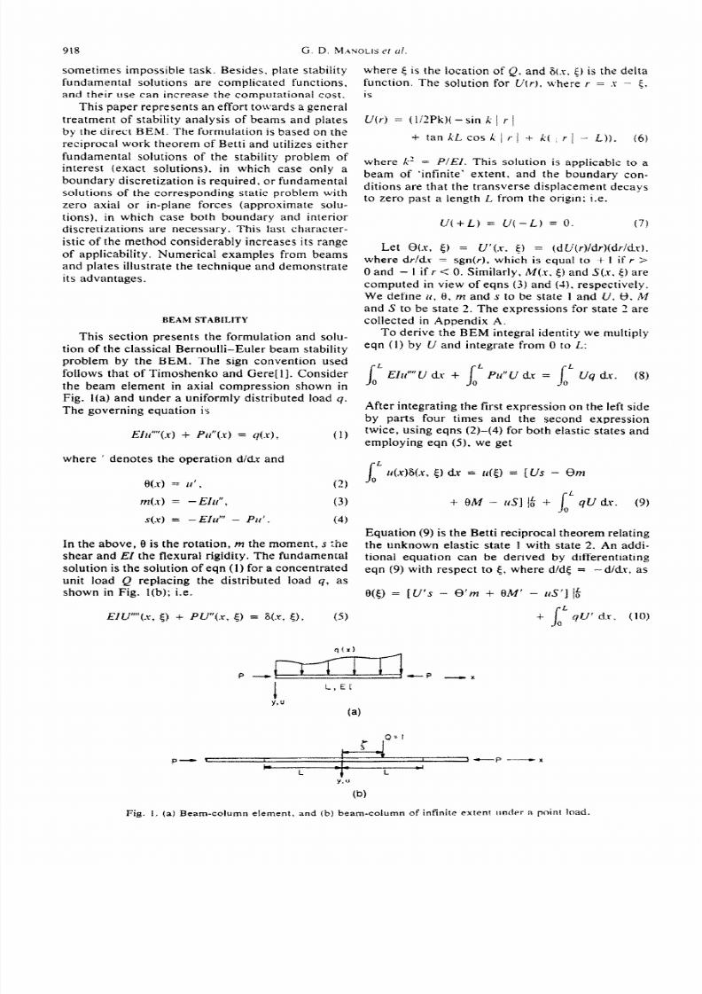
This section presents the formulation and solu-tion of the classical Bernoulli-Euler beam stabilityproblem by the BEM. The sign convention usedfollows that of Timoshenko and Gere[ 11. Considerthe beam element in axial compression shown inFig. I(a) and under a uniformly distributed load 4.

The governing equation is

EZlr”“(X) + Plr”(X) = q(x), (1)

To derive the BEM integrai identity we multiplyeqn (I) by U and integrate from 0 to L:

After integrating the first expression on the left sideby parts four times and the second expressiontwice, using eqns (Z)-(4) for both elastic states andemploying eqn (51, we get

where ’ denotes the operation didx and

0(x ) = l f ’ , (2) IaL tW%x, 5) dr = u([) = {Us - 8m

m ( x ) = -EM’ , (3) f BM - US] 10” I,” qU dy. (9)

S(X) = - Elu” - Pd. (4)Equation (9) is the Betti reciprocal theorem relating

In the above, 9 is the rotation, m the moment, s :he the unknown elastic state I with state 2. An addi-shear and El the flexural rigidity. The fundamentai tional equation can be derived by differentiatingsolution is the solution of eqn (1) for a concentrated eqn (9) with respect to {, where d/de = -d/dr, asunit load Q replacing the distributed load 4, asshown in Fig. l(b); i.e. e(k) = [U’s - W m + B M - f f . S’ j I i

L

EIu ” ‘ ( .r, 5 ) f Pu” (x , 5 ) = 6 (x , Q , f 3 f q U ’ dr, (10)

P-W

I L,ETY*U

(4

P P x

YbJ

(W

Fig. I. (a) seam-column element. and (b) beam-column of infinite extent under a point load.



Beam and plate stability 919

where U’, 0’. M’ and S’ are also given in AppendixA. All that remains is to evaluate eqns (9) and (10)at 5 = L - E and at 5 = 0 + e as z -, 0. This yieldsa 4 x 4 system of equations

where column vector fi = [u(L), l{(O)] , the sub-matrix

[

L/(L.L) 1 UO. L)i l l- - - -- - - -U L.) U O,)+ 12)and similarly for the remaining expressions.

The method for solution is similar to the one em-ployed in the FEM[3], where a generalized dis-placement vector is related to a generalized loadvector through the usual flexural stiffness matrixplus a geometric stiffness matrix,in which the axialload P appears as a parameter. Equation (11) istherefore written for all beams composing the struc-ture, and a global matrix equation is thus obtainedby superposition. For the computation of bucklingloads, the term containing the distributed load 9 isneglected. Upon application of the boundary con-ditions, a composite matrix is obtained whose de-terminant must vanish. This leads to a transcen-dental equation whose first root is the critical load,and subsequent roots yield the remaining bucklingloads. For small-sized problems, an iterative ap-proach using the false position method to minimizethe number of iterations is adequate[ 161.

In the above formulation, one may use the fun-damental solution n of the flexural problem as anapproximation; i.e. solve

E1VYx, 5) = 6(X, 5)

in lieu of eqn (5). For this case

(13)

D(r) = (L3/12Ef)(2 + ( ( r ) lL)3 - 3( ) r ( /L)‘),

(14)

which has the same boundary conditions as before:

i.e. U(L) = U(-L) = 0. The corresponding ro-tation, moment, and shear associated with g(r). aswell as the first derivatives of these quantities thatdefine elastic state 2, are also collected in AppendixA. As far as the BEM formulation using u(r) isconcerned, the difference comes in deriving eqn (9)where we have the term

I

L

= u Q + Pu’i7” dr ( IS)0

instead of just rr(Q as before. This implies that the

right sides of eqns (9) and (10) need to be augmentedby the terms

P

respectively. It is precisely these terms that giverise to the interior discretization. We now need toconsider beam elements that are ‘small’ enough toallow for a linear variation of the transverse dis-placement between the end nodes. Thus, the aboveintegrals of I/“(r) = (L/2EI) ( 1 r/L ( - 1) and V’(r)= (1/2El)sgn(r) over the length can easily be eval-

uated analytically. Other than that, the numericalprocedure used in conjunction with the exact fun-damental solutions of the buckling problem remainsunchanged and can be used here as well.

PLATE STABILITY

This section develops the BEM as applied to thin(Kirchhoff) plate theory. Once more, the sign con-vention of Ref. [I] is adopted. The governing equa-tion for plate buckling in Cartesian coordinates is

DV4w - N, +N,? $

where rrp(x, y) is the transverse deflection, D theplate’s flexural rigidity, Nij(X, y) the in-planeforces, 9(.r, y) the distributed load, and r is the deloperator. The moments per unit length and theshears are defined as

Mij = -D[(I - U)Mf,ij+ UW+kk 6;j] 18)

and

Qi = Mij.jq (19)

respectively, where v is Poisson’s ratio, and Sij isthe Kronecker delta. Also, repeated symbols in theindicial notation used above imply summation, andthe index following a comma denotes spatial dif-ferentiation. The in-plane forces are assumed to re-main unchangea during bending and obey the fol-lowing equations of equilibrium:

%+aN,,. aN.r,. aN,.,-~-+~---_~o.

ay a.r ay(20)

For simplicity we assume that N,, = N,., = N. N.,= 0. and, for generality, we introduce an orthog-onal system (n, t). n being the normal and t thetangent to the plate’s perimeter S. Equation ( 17)can



91-o G. D. MWOL S et d

be condensed to read

DC K~ NC’,,’ = 4. (21)

Betti’s reciprocal theorem for two elastic stateshas the form

qw*64 c J VW* - MB’) dssA

=A

where

e2,

bf= +u ,aiM,,V=Qn+ a

,= 2 + (2

M*e) ds

(22)

- u) 2 , (23)

T = D(1 - u)a’ I&’ a21

- - -an2at, anaf,

In eqn (23), 8 is the rotation, V is known as theKirchhoff shear, and T denotes the jump in thetwisting couple at corner 1. Furthermore, the nor-mals and tangents on one side of the corner aredenoted by subscript 2 and on the other side by

subscript 3. We will assume that the perimeter ofthe plate is smooth so that there is no summationover L, the total number of corners, in eqn (22). Ifthe starred state (*) is identified as the solution of(21) for a unit point force S(s. 7) replacing 9, theneqn (22) becomes

cd& 7$ = I (- wv* + tM4* - Me*s

+ VW*) ds

(24)

If point (5, n) is on the perimeter 5, c = 0.5. andif (5, q) is inside the area A, c = 1.0. A secondintegral equation is generated by taking rv’([, Y)).’ = a/an, where nl is the normal at the load point

(5. n). Thus.

T 8~“) ds -0

q\~.” dA..i

(2’)

Equations (2-l) and (25) are the counterparts of eqns(9) and (10) in plate buckling. The difference is thatthe boundary S must now be discretized into a num-ber of line elements, while in beam buckling thebeam segment between two nodes plays the role of

a line element. Note that the area integrals in botheqns (24) and (25) are not considered if only thecritical load is sought. Finally, if r* is the solutionof the flexure problem, i.e. DG * = S, then theright sides of eqns (24) and (25) must be augmentedby the terms

IINY%*dA and

IIh’Y%*‘dA. (‘61

A A

respectively. Again, it is these area integrals thargive rise to an interior discretization using area ele-ments.

The fundamental solution for pure flexure is ob-tained from solving for the transverse displacementof a circular plate with a concentrated load at thecenter. This is an axisymmetric problem and from[I] we have

i?*(r) = (1/167iD) (r2 In r2 - G), (271

where r2 = (.r - 5)’ -+ (T - 9)‘. Note that thedisplacement-is finite at r = 0 and decays to zeropast r = v’e, where e is the base of the naturallogarithm. Similarly, the exact solution II.* is ob-tained from the same problem with the addition ofan in-plane compressive radial force N at the pe-rimeter of the plate. Consulting [l-t]. we have

r\‘*(r) = (DihrN) (In r + K, \‘a). (28,

where K. is the modified Bessel function of orderzero. Expressions for i7*. -* , zx. v* and i?‘. G*‘.-@I , y*’ are collected in Appendix B. Similarexpressions can be derived for I(.-. 0”. and so on.by noting the recurrence relations for Bessel func-tions and their derivatives: i.e.

dK&-)- = -K,(r).d’Ko(r)

dt- = Kz(r),

dr’

d’K&)- = -K’(r).

d’Ko(r)dr’

- = K4(r).dr’



Beam and plate stabili:y 921

and 29)KM = ZIrKl r) f Kdr),

K3W = 4MKzW + K, r).

K.,(r) = (6/r)K,(r) + Kz(r).

Note that the subscript denotes the order of theBessel function, and that it is possible to expressall the derivatives of K”(r) in terms of K&I andK,(r) only. The expressions for the elastic state )I**are also collected in Appendix B.

NUMERIC L TRE TMENT

A few comments about the numerical imple-mentation of the BEM are collected here. As far as

beam buckling is concerned, the only remark is thatno numerical integrations are required. For theplate buckling case, two types of line elements areused for the discretization of the plate’s perimeter:(a) constant elements, where all boundary quan-tities (displacement, rotation, moment, and shear)are assumed to remain constant over the elementand are collocated at a node in the center; and (b)linear elements, defined by two nodes placed at theendpoints of the element and over which the bound-ary quantities vary in a linear fashion. For the caseof a closed boundary, both types of elements resultin the same number of nodes, and the only differ-ence is in the coefficient matrices [A], [B], and [Clthat result from a standard nodal collocation: i.e.

c {f} = [Al {;} +[Bl{+}

+ {D(N)} + {E(q)). (30)

In the above equation, the column matrices [w, 0J T

and [M, V] T contain the nodal values of the ob-vious boundary quantities, and coefficient matrices[A 1, [B], and [C] result from integrating the appro-priate fundamental solutions [see eqn (24) and (ZS)]over the perimeter S. Also, if the approximate fun-damental solutions are to be employed, column ma-trix {D} must be included [see eqn (2611, and if theplate supports any concentrated or distributedloads, column matrix {E} must be included.

For the case of linear elements in conjunctionwith the approximate (flexural) fundamental solu-tions, we used the expressions obtained by exactlyintegrating the kernels over an element[l7]. In thecase of constant elements we used standard four-point Gaussian quadrature. When singular casesarise, i.e. when a receiving node coincides with thenode defining the element over which integration isbeing performed, the integrals remain finite. Thus,no special precautions are needed other than;to sub-divide the constant element into two parts, one tothe left and one to the right of the singular node. Astandard four-point quadrature is then applied to

each subelement. and the results are added. Sincethe answers obtained from some plate flexure prob-lems using discretizations based on only constantand only linear elements were nearly identical, con-stant elements coupled with Gaussian quadraturewere subsequently employed for the integration ofthe exact fundamental solutions over the boundary.

In order to compute {D} and/or {E}. area ele-ments must be introduced. We used three-node tri-angles and collocated at the center of each triangle.Both quadratic and quintic quadrature schemeswere employed. A singular area element ariseswhen one side of a triangle coincides with the sin-gular line element. No problems are encountered inthis case as long as the quadrature scheme used forthe triangle does not include gauss points that co-incide with the singular node. lLlore details can befound in Ref. [18].

NUMERIC L EX MPLES

As far as beam-column stability is concerned.the following cases were considered: (a) simply sup-ported beam-the critical load is P,, = n’ EIIL’).For a beam with EIIL’ = I, P,, = T’ = 9.8696 lb.Using the exact fundamental solution we get P,, =9.8707 lb after eight iterations, an answer that is0.01% in error. The same error level is obtained by

using the approximate fundamental solution if thebeam is subdivided into six segments; (b) cantileverbeam-for the same material and geometric prop-erties as above, P,, = ~“14 = 2.4674 lb. After I7iterations the formulation with the exact funda-mental solution gave P,, = 2.4829 lb, which is 0.6%in error. Using four elements in conjunction withthe approximate fundamental solution gave an errorof 0.01%; (c) propped cantilever-here P,, = 20. I9lb, and the exact fundamental solution formulationgave P,, = 20.188 lb after seven iterations. which

is 0.05% in error. The other formulation requiredfive elements in order to obtain the same error level.For such small problems, computer execution timerequirements are minor. Similar studies concerningthe FEM can be found in Ref. [2].

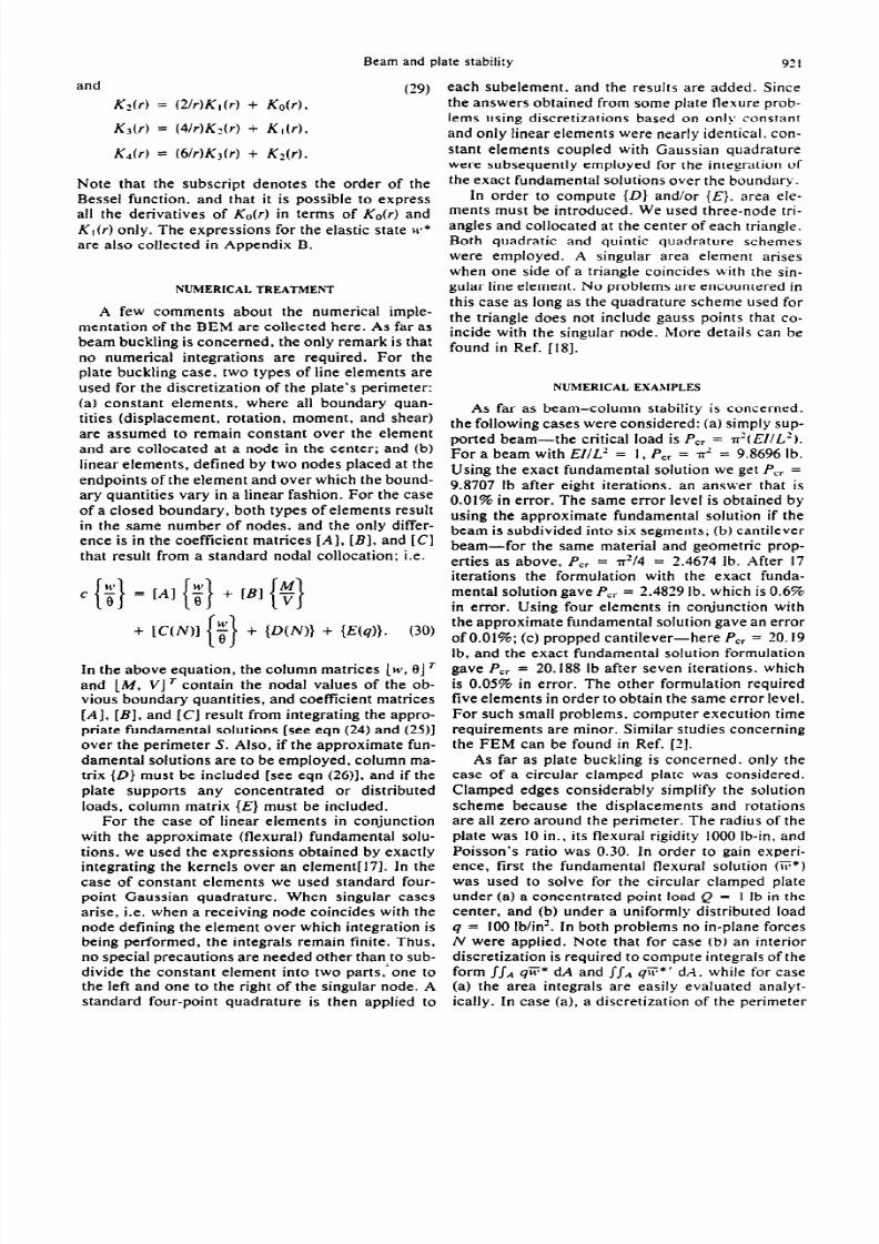
As far as plate buckling is concerned. only thecase of a circular clamped plate was considered.Clamped edges considerably simplify the solutionscheme because the displacements and rotationsare all zero around the perimeter. The radius of theplate was 10 in., its flexural rigidity 1000 lb-in. andPoisson’s ratio was 0.30. In order to gain experi-ence, first the fundamental flexural solution (51;*)was used to solve for the circular clamped plateunder (a) a concentrated point load Q = I lb in thecenter, and (b) under a uniformly distributed load9 = 100 lb/in’. in both problems no in-plane forcesN were applied. Note that for case (b) an interiordiscretization is required to compute integrals of theform JJA 9S;;* dA and JJA 91i;*’ dA. while for case(a) the area integrals are easily evaluated analyt-ically. In case (a), a discretization of the perimeter



G. D. MANOLI S et ul

ty

a(4

(W

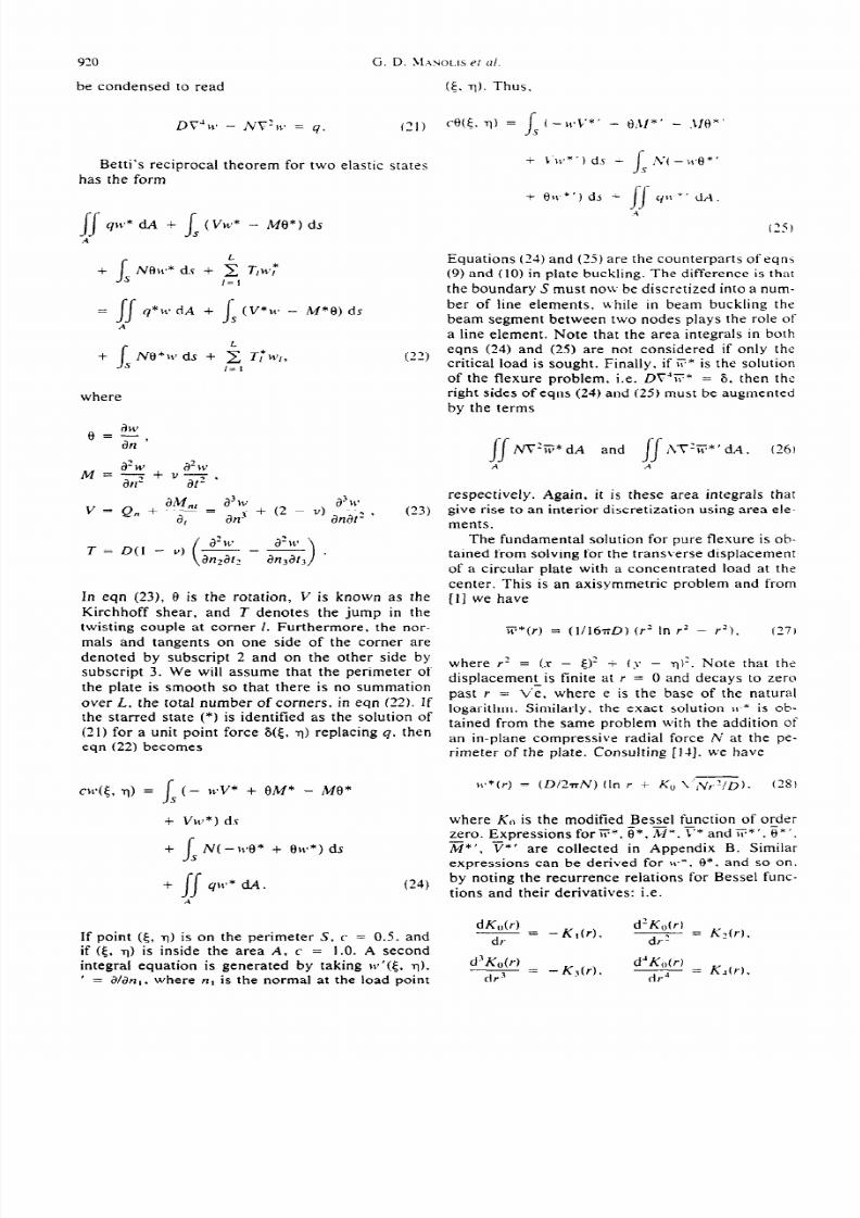
Fig. 2. (a), (b) Typical boundary and interior discretizationpatterns for circular clamped plate.

into 24 constant elements gave a moment at the

boundary of M = -0.8128 lb, and a discretizationinto 24 linear elements gave M = - 0.7924 lb. Theanalytic solution[ l] is M = - P/4n = - .07958 lb.Thus, the first answer is 2.1% in error, and the sec-ond one is 0.4% in error. In the second case, twointerior discretization patterns employing 3-nodetriangles were used: the coarse one (six elementsper quadrant) is shown in Fig. 2(a), and the fine one(12 elements per quadrant) is shown in Fig. 2(b).Compared to the analytic solution for the normaledge moment of M = -qa’/8 = - I250 lb, the 24

constant-element discretizations with the coarseand fine interior meshes gave answers 4.2% and2.9% in error, respectively, while the 24 linear-ele-ment discretizations with the coarse and fine inte-rior meshes gave answers 3.4% and 1.8% in error,respectively. Obviousiy, the plate discretizationpatterns which gave the best results in the flexuralproblems were used for the buckling problem. Theexact critical load is N,, = 14.68 D/u’ = 146.8 lb/in[l]. Compared to that. the approximate funda-mentaf solution formulation was 3.2% in error, andthe exact one was 2.1% in error. In both cases morethan I5 iterations were required for convergence.It should be added that the quadratic scheme wasused for integrating over triangles, and constant lineelements were employed in the buckling problem.Also, computer time and memory requirements forthese problems are very modest.

CONCLUSlONS

The buckling of slender beams and thin platesby the boundary element method was presented. It

is not surprising that both beam formulations yieldvery accurate results. This is so because no nu-merical quadrature is required. and all relevantquantities are analytically evaluated. In the plateformulations. however. quadrature is required, andthe integrands exhibit mild (integrable) singulari-ties. Nonetheless, the critical loads are computedwith acceptable accuracy. The results obtained b ,using approximate fundamental solutions are notvery different from those obtained by using the cor-rect fundamental solutions, provided the interior isadequately discretized.

The plate formulation can easily be expanded totackle probtems involving thick plates or plates es-hibiting anisotropy, provided the appropriate fun-damental solutions are available.

AcknowlecIggment-The authors thank the UniversityComputing Services for making their CDC Cyber 730available to them.

REFERENCES

1 S. P. Timoshenko and J. IM. Cere. Theory ofEhricStability. McGraw-Hill, New York i 1961).

2. R. H. Gallagher, Fini re Nement Anal ysis: Fanda-mentals. Prentice-Hall, Englewood Cliffs (1975).

3, A. Ghali and A. M. Neville. ~r~z~cr~~~u~ n&is: AUnified CIassicat and ,Varri.r Approach. Chapmanand Hall, London (1978).

4 P. K. Banejee and R. Butterfield. Boandar? ElemenrM ethod s i n Engineeri t l g Sci ence. McGraw-Hill, Lon-don (1981).

5. M. A. Jaswon and M. Slaiti. An integral equation for-mulation of plate bending problems. J. Engtrg Mnfh.2, 83-93 (1982).

6. M. Maiti and S. K. Chakrabarty. Integral solutions forsimply-supported polygonal plates. Int. J. Engng Sci.12, 793-806 (1974)..

7. N. J. Altiero and D. L. Sikarskie. A boundary integralmethod applied to plates of arbitrary plan form. COWplir. Stntcr. 9, 163-168 t 19781.

8. D. J. Forbes and A. R. Robinson. Numerical analysisof elastic plates and shallow shells by an integral equa-tion method. Structural Research Series Report 345.University of Illinois, Urbana (1969).

9. G. Bezine. Boundary integral formulation for plateflexure with arbitrary boundary conditions. lMecll.Res. Comm an. 5, 197-206 (1978).

IO. M. Stern, A general boundary integral formulation forthe numerical solution of plate bending problems. inr.J. So/id s Smrcr. 15, 769-782 (1979).

II. M. Brunet, An integral equation method for bucklineanalysis of thin walled non-uniform tapered members.in Recent Ad vances i n Boundary Elemenr Sl eri mds.(Edited by C. A. Brebbia). pp. 317-315. PentechPress, London (1979).T. Sekiya and T. Katayama, ;\nalysis of buckling

using the influence function. Proc. 29th Japan h’n-ii onui Congress of Appi ied ,\ fechanics. pp. 25-31(1979).H. Tai, T. Katayama and T. Sekiya. Buckling analysisby influence function. .Lfec/r. Res. Commlrn. 9, l39-144 1982).Y. Niwa, S. Kobayashi and M. Kitahara. Determi-nation of eigenvalues by boundary element methods.in Devefopmcnts in Bol~nd~l~ Element Merhods--2.(Edited b; P. K. Banerjee and R. P. Shawl, pp. lf3-176. ADolied Science Publishers. London (1987).G. Go&odinov and D. Ljutskanov. The boundary ele-ment method applied to plates. Appt. Marh. RlodeIli ng6, 237-7-4-1 (1982).

12.

13.

II.

15.



Beam and plate stability 923

16. C. E. Froberg. Inrroducrion to Numerical Analysis,2nd ed. Addison-Wesley. Reading, Mass. (1973).

17. H. Tottenham, The boundary element method forplates and shells, in Developmcnrs in Borrnda~ Ele-ment Merho -/, (Edited by P. K. Banerjee and R.P. Shaw), pp. 173-205. Applied Science Publishers,

London (1979).18. M. F. Pineros, Beam and Plare Stability by Bounda?Element Method. Master Project. State University ofNew York, Buffalo (1983).

19. M. Abramowitz and 1. Stegun. Handbook o Mathe

matical FuncGons. Dover. New York (1972).

APPENDIX A. BEAM FUNDAMENTAL SOLUTIOSS

The approximate fundamental solutions that constitutestate 2 for the case of beam buckling are listed below.

E(r) = (L’IIZEI)(Z + ( r/L 1’ - 3 ( r/L 1’1,

G(r) = (L’/4EI) 1 /L 1 I r/L 1 - 2) sgn(r),

X?(r) = (L/2) (I - I r/L I ),

S(r) = - 4 sgn(r),

Cl’(r) = --G(r),

8’(r) = - (6L112EI) ( I r/L ) - I),

M’(r) = # sgn(r),

S’(r) = 0,

where ’ here is d/d{ = - d/dr.The exact fundamental solutions for the same problem

are

U(r) = (1/2Pk)(-sink]rI + tankLcoskIr1

+ k( ) r ( - L)).

8(r) = (1/2P)(-cosklrl - tankLsinkIr1

+ 1) sgn(r).

M(r) = (-1/2k)(-sinkIr/ + tankLcosk/rI).

S(r) = - 1 sgn(r),

U’(r) = - B(r),

8’(r) = (k/2P) (-sin k ) r 1 + tan kL cos k I r 1 ).

M’(r) = 1 (cos k I r ( + tan kL sin k ( r [ ) sgn(r).

S’(r) = 0.

APPENDIX B. PLATE FUNDAMENTAL SOLUTIONS

For plate buckling. the approximate fundamental so-lutions are

H’* = (1116nD)I r’logr’ - rZ (.

8* = (l/16nD)2rlogrZcos/3,

M* = (l/ )J (I + v)(I + log?) + (I - v)cos2@ I.

V* = (1/8nr)l (5 - u)cosf3 + (I - U)COS~~ 1,

H’*’ = - (1/8aD)rlogr’cosa.0*’ = - (1/8aD)J (I + logr’)cos(a - /3)

+cos(a+p)I.

M*’ = - (IWrrr)J 2(I + v)cosa

+ (1 - v)(cos( 3 - a) - cos(2p + aI) 1,V*’ = + (l/8&)( (5 - v)cos(a + p)

+ 2(I - v)cos(3p + a) - (I - v)cos(3p - h) I.

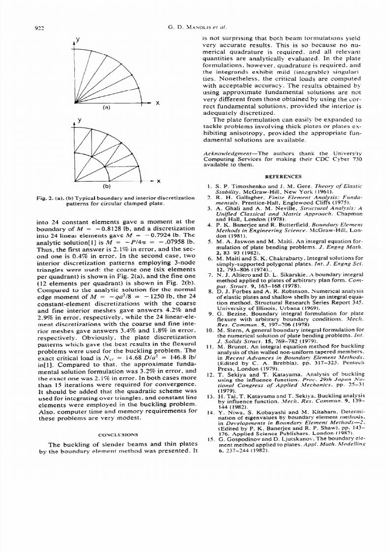
The above equations are taken from Ref. [l7]. Asshown in Fig. 3, p is the angle between the normal atreceiver (x. _v) and the line connecting (x. _v) with the source

Fig. 3. Plate geometry details.

(5, $. while a is the angle between the normal at (4, 11)and that line.

The exact fundamental solutions for plate buckling canbe synthesized from the following expressions:

w = a [In r + Ko],

where ?T2 = NID a = lIZaT’ and Ko = Ko( 3r) KI =K,(Tr) are evaluaied from expiessions given in Re;. [191.Furthermore,

aw aw ar

sn=

--

ar an ’a2w a2w ar 2+__0 aw a’r

an2=ar2 an ar an2 ’

a a3w ar 3

0

~ 3 a2w a’r ar a $’ a’r

an)=ar) an---+ --ar2 an2 an ar an’ ’

where, for instance,

ar ar ax ar ay-_=--+---‘cospan ax an ay an

a2r1sin2 p

S r

and p was identified above. The expressions involving thetangential derivatives dwldr, etc.. are derived from theones involving the normal derivatives (awlan. etc.) by sim-ply replacing n by 1. The only difference is that

ar- = sin p.

a?r

alicosZ p.s=r

Using all the above expressions in eqn (23) yields 8, Mand V. The remaining expressions are obtained as IV =aw4an,. 8’ = -aelan,. M’ = -aMIan, and V’ = -avldnl. where n, is the normal at the source (6, ?).

manolis,gd, beskos, de 1986

Documents