managerial economicsmanagerial economics d.j. reyniers mn3028, 2790028 2011 undergraduate study in...
TRANSCRIPT

Managerial economicsD.J. ReyniersMN3028, 2790028
2011
Undergraduate study in Economics, Management, Finance and the Social Sciences
This is an extract from a subject guide for an undergraduate course offered as part of the University of London International Programmes in Economics, Management, Finance and the Social Sciences. Materials for these programmes are developed by academics at the London School of Economics and Political Science (LSE).
For more information, see: www.londoninternational.ac.uk

This guide was prepared for the University of London International Programmes by:
Prof D.J. Reyniers, Director, Interdisciplinary Institute of Management, and Professor ofManagement, London School of Economics and Political Science, University of London.
This is one of a series of subject guides published by the University. We regret that due to pressure of work the author is unable to enter into any correspondence relating to, or arising from, the guide. If you have any comments on this subject guide, favourable or unfavourable, please use the form at the back of this guide.
University of London International Programmes
Publications Office
Stewart House
32 Russell Square
London WC1B 5DN
United Kingdom
Website: www.londoninternational.ac.uk
Published by: University of London
© University of London 2006
Reprinted with minor revisions 2012
The University of London asserts copyright over all material in this subject guide except where otherwise indicated. All rights reserved. No part of this work may be reproduced in any form, or by any means, without permission in writing from the publisher.
We make every effort to contact copyright holders. If you think we have inadvertently used your copyright material, please let us know.

Contents
i
Contents
Introduction ............................................................................................................ 1
Aims and objectives ....................................................................................................... 1Subject guide breakdown .............................................................................................. 1Learning outcomes ........................................................................................................ 2Reading ........................................................................................................................ 2Mathematics for managerial economics ......................................................................... 3Online study resources ................................................................................................... 3Examination advice........................................................................................................ 4Some advice and ideas on how to study ......................................................................... 5Glossary of abbreviations ............................................................................................... 5
Chapter 1: Decision analysis ................................................................................... 7
Aims ............................................................................................................................. 7Learning outcomes ........................................................................................................ 7Essential reading ........................................................................................................... 7Introduction .................................................................................................................. 7Decision trees ................................................................................................................ 8Attitude towards risk ................................................................................................... 10Some applications ....................................................................................................... 12The expected value of perfect information .................................................................... 14A reminder of your learning outcomes .......................................................................... 17Sample exercises ......................................................................................................... 17
Chapter 2: Game theory ....................................................................................... 19
Aims ........................................................................................................................... 19Learning outcomes ...................................................................................................... 19Essential readings ........................................................................................................ 19Further reading ............................................................................................................ 19Introduction ................................................................................................................ 20Extensive form games .................................................................................................. 21Normal form games ..................................................................................................... 23Nash equilibrium ......................................................................................................... 25Prisoners’ dilemma ...................................................................................................... 29Perfect equilibrium ....................................................................................................... 30Perfect Bayesian equilibrium ........................................................................................ 32A reminder of your learning outcomes .......................................................................... 34Sample exercises ......................................................................................................... 34
Chapter 3: Bargaining ........................................................................................... 37
Aims ........................................................................................................................... 37Learning outcomes ...................................................................................................... 37Essential reading ......................................................................................................... 37Further reading ............................................................................................................ 37Introduction ................................................................................................................ 37The alternating offers bargaining game ........................................................................ 38Incomplete information bargaining .............................................................................. 39A reminder of your learning outcomes .......................................................................... 40Sample exercise ........................................................................................................... 40
28 Managerial economics
ii
Chapter 4: Asymmetric information ..................................................................... 41
Aims ........................................................................................................................... 41Learning outcomes ...................................................................................................... 41Essential reading ......................................................................................................... 41Further reading ........................................................................................................... 41Introduction ................................................................................................................ 42Adverse selection ........................................................................................................ 42Moral hazard ............................................................................................................... 45Signalling and screening .............................................................................................. 47Principal-agent problems ............................................................................................. 50Effort cannot be observed ............................................................................................ 52A reminder of your learning outcomes .......................................................................... 54Sample exercises ......................................................................................................... 54
Chapter 5: Auction and bidding ............................................................................ 57
Aims ........................................................................................................................... 57Learning outcomes ...................................................................................................... 57Essential reading ......................................................................................................... 57Further reading ............................................................................................................ 57Introduction ................................................................................................................ 58Private and common value auctions ............................................................................. 59Private value auctions and their ‘optimal’ bidding strategies ........................................ 60Auction revenue .......................................................................................................... 65Common value auctions .............................................................................................. 65Complications and concluding remarks ........................................................................ 67Conclusion .................................................................................................................. 71A reminder of your learning outcomes .......................................................................... 71Sample exercises ......................................................................................................... 71
Chapter 6: Topics in consumer theory .................................................................. 73
Aims ........................................................................................................................... 73Learning outcomes ...................................................................................................... 73Essential reading ......................................................................................................... 73Further reading ............................................................................................................ 73Introduction ................................................................................................................ 74Reviewing consumer choice ......................................................................................... 74Consumer welfare effects of a price change ................................................................. 78Elasticity ...................................................................................................................... 79State-contingent commodities model ........................................................................... 81Intertemporal choice .................................................................................................... 83Labour supply .............................................................................................................. 86Risk and return ............................................................................................................ 90A reminder of your learning outcomes .......................................................................... 93Sample exercises ......................................................................................................... 94
Chapter 7: Production, factor demands and costs ............................................... 97
Aims ........................................................................................................................... 97Learning outcomes ...................................................................................................... 97Essential reading ......................................................................................................... 97Further reading ............................................................................................................ 97Introduction ................................................................................................................ 97Production functions and isoquants ............................................................................. 98Firm demand for inputs.............................................................................................. 101
Contents
iii
Case: monopsony and minimum wages ...................................................................... 105Industry demand for inputs ........................................................................................ 106From production function to cost function .................................................................. 109Division of output among plants ................................................................................ 110Estimation of cost functions ....................................................................................... 112A reminder of your learning outcomes ........................................................................ 113Sample exercises ....................................................................................................... 113
Chapter 8: Topics in labour economics ............................................................... 115
Aims ......................................................................................................................... 115Learning outcomes .................................................................................................... 115Further reading .......................................................................................................... 115Introduction .............................................................................................................. 116Efficiency wages ........................................................................................................ 116Case: Politicians, sleaze and efficiency wages ............................................................. 119Firm demand for labour ............................................................................................. 121Internal labour markets .............................................................................................. 123Why do wages rise over a career path? ...................................................................... 123Managerial and executive pay .................................................................................... 127A reminder of your learning outcomes ........................................................................ 128Sample exercises ....................................................................................................... 129
Chapter 9: Market structure ............................................................................... 131
Aims ......................................................................................................................... 131Learning outcomes .................................................................................................... 131Essential reading ....................................................................................................... 131References cited ........................................................................................................ 131Introduction .............................................................................................................. 132Determinants of market structure ............................................................................... 132Strategy of incumbents .............................................................................................. 133Measures of market structure ..................................................................................... 135Perfect competition .................................................................................................... 136Case: Competition in the insurance industry ............................................................... 137Monopoly .................................................................................................................. 139Monopolistic competition .......................................................................................... 141A reminder of your learning outcomes ........................................................................ 144Sample exercises ....................................................................................................... 144
Chapter 10: Monopolistic pricing practices ....................................................... 147
Aims ......................................................................................................................... 147Learning outcomes .................................................................................................... 147Essential reading ....................................................................................................... 148Further reading .......................................................................................................... 148Introduction .............................................................................................................. 149Price discrimination ................................................................................................... 149Second degree price discrimination ............................................................................ 152Third degree price discrimination................................................................................ 154Case: The European car market .................................................................................. 157Case: Yield management ............................................................................................ 161Commodity bundling ................................................................................................. 163Multiproduct firms ..................................................................................................... 167Transfer pricing .......................................................................................................... 171Case: Transfer pricing and taxation ............................................................................. 176
28 Managerial economics
iv
A reminder of your learning outcomes ........................................................................ 177Sample exercises ....................................................................................................... 178
Chapter 11: Oligopoly ........................................................................................ 181
Aims ......................................................................................................................... 181Learning outcomes .................................................................................................... 181Essential reading ....................................................................................................... 181Further reading .......................................................................................................... 181Introduction .............................................................................................................. 182Strategic asymmetry .................................................................................................. 185Stackelberg ............................................................................................................... 185Symmetric models ..................................................................................................... 188Bertrand .................................................................................................................... 190Collusion ................................................................................................................... 192Case: OPEC ............................................................................................................... 194Case: Diamonds ........................................................................................................ 195Dynamic interaction ................................................................................................... 195Case: Aluminium ....................................................................................................... 197Conclusion and extensions ......................................................................................... 198A reminder of your learning outcomes ........................................................................ 199Sample exercises ....................................................................................................... 199
Appendix 1: Sample examination paper ............................................................ 201
Appendix 2 References for older versions of textbooks .................................... 207
Chapter and page references for older books ............................................................. 207
Appendix 3: Maths checkpoints ......................................................................... 211
1. Functions – a few general remarks ......................................................................... 2112. Differentiation ....................................................................................................... 2123. Logarithmic functions / properties of In and exp. ..................................................... 2144. Integration ............................................................................................................ 2145. Systems of equations / manipulating equations ...................................................... 2156. Uniform distribution ............................................................................................... 2167. Probabilities ......................................................................................................... 2168. The discount factor ‘δ’ ............................................................................................ 2189. The company’s profit function ................................................................................. 219General suggestions for studying and revising ............................................................ 220Overview and definitions of some important functions ................................................ 22010. A few hints on solving questions .......................................................................... 221
Introduction
1
Introduction
Aims and objectivesThis course is intended as an intermediate economics paper for BSc (Management) and BSc (Economics) students. As such, it is less theoretical than a microeconomic principles course and more attention is given to topics which are relevant to managerial decision-making. For instance, business practices such as transfer pricing, tied sales, resale price maintenance and exclusive dealing are analysed. Topics are presented using equations and numerical examples, that is, an analytical approach is used. The theories which are presented are not practical recipes; they are meant to give you insight and train your mind to think like an economist.
Specification of the course are to:
• enable you to approach managerial decision problems using economic reasoning
• present business practice topics using an analytical approach, using equations and numerical insight.
Why should economics and management students study economics? The environment in which modem managers operate is an increasingly complex one. It cannot be navigated without a thorough understanding of how business decisions are and should be taken. Intuition and factual knowledge are not sufficient. Managers need to be able to analyse, to put their observations into perspective and to organise their thoughts in a rigorous, logical way. The main objective of this paper is to enable you to approach managerial decision problems using economic reasoning. At the end of studying this subject, you should have acquired a sufficient level of model-building skills to analyse microeconomic situations of relevance to managers. The emphasis is therefore on ‘learning by doing’ rather than reading and essay writing. You are strongly advised to practise problem-solving to complement and clarify your thinking.
Subject guide breakdownThe coverage in this subject guide is close to what I teach my second year BSc (Management) students at the London School of Economics:
• basic microeconomics (i.e. consumer theory, labor supply, neoclassical theory of the firm, factor demands, competitive structure, government intervention, etc)
• some newer material regarding efficiency wages, incentive structures, human resource management, etc
• individual (one person) decision-making under uncertainty and the value of information; the theory of games. The latter considers strategic decision-making with more than one player and has applications to bargaining, bidding and auctions, oligopoly and collusion
• the effects of asymmetric information (one decision-maker has more information than the other)
• Akerlof’s ‘lemon’ model which explains the disappearance of markets due to asymmetric information
• situations of moral hazard (postcontractual opportunism) and adverse selection (precontractual opportunism).
28 Managerial economics
2
Learning outcomesAt the end of the course, and having completed the Essential reading and exercises, you should be able to:
• prepare for Marketing and Strategy courses by being able to analyse and discuss consumer behaviour and markets in general
• analyse business practices with respect to pricing and competition
• define and apply key concepts in decision analysis and game theory.
Reading
Essential readingThis guide is intended for intermediate level courses on economics for management. It is more self-contained than other subject guides might be. Having said this, I do want to encourage you to read widely from the recommended reading list. Seeing things explained in more than one way should help your understanding. In addition to studying the material, it is essential that you practise problem-solving. Each chapter contains some sample questions and working through these and problems in the recommended texts is excellent preparation for success in your studies. You should also attempt past examination questions from recent years; these are available online. Throughout this guide, I will recommend appropriate chapters in the following books.
Tirole, J. The theory of Industrial Organisation. (Cambridge, Mass: The MIT Press, 1988) [ISBN 9780262200714] this is excellent for the second part of the guide dealing with pricing practices and strategic interactions.
Varian, H.R. Intermediate Microeconomics. (New York: W.W. Norton and Co., 2006) seventh edition [ISBN 9780393928624] this can be useful mainly for the review part of the course and those who prefer a less mathematical treatment
Note on older editions: most of the relevant material from Varian (2006) can also be found in the sixth edition of this book. Relevant chapters for older edition are listed in Appendix 2.
Detailed reading references in this subject guide refer to the editions of the set textbooks listed above. New editions of one or more of these textbooks may have been published by the time you study this course. You can use a more recent edition of any of the books; use the detailed chapter and section headings and the index to identify relevant readings. Also check the virtual learning environment (VLE) regularly for updated guidance on readings.
Further readingWe list a number of journals throughout the subject guide which you may find it interesting to read.
Please note that as long as you read the Essential reading you are then free to read around the subject area in any text, paper or online resource. You will need to support your learning by reading as widely as possible and by thinking about how these principles apply in the real world. To help you read extensively, you have free access to the VLE and University of London Online Library (see below).
Introduction
3
Mathematics for managerial economicsThe mathematical appendix gives an indication of the level of mathematics required for the course. Review it! If you are having difficult with the mathematics in this course, you might find the following book useful.
Ivan, P.N.G. Managerial Economics. (London: Blackwell Publishers, 2001/02) second edition [ISBN 9780631225164 (hbk 2001), 97801405160476(pbk 2007)].
It does not assume a prior knowledge of economics and offers a less mathematical introduction to managerial economics. However, it is recommended as preliminary reading only and should not be used as a substitute for the subject guide. The level of mathematics it uses is much lower than that required for this course and it does not cover the topics in detail. The different models are treated in a very basic way. It can, however, be a useful back-up reference if you don’t have the basic knowledge required to understand a topic. In particular, if you use this book, it is recommended that you work through the mathematical appendices which are provided at the end of each chapter. It is not necessary to study the entire book.
Online study resourcesIn addition to the subject guide and the Essential reading, it is crucial that you take advantage of the study resources that are available online for this course, including the VLE and the Online Library.
You can access the VLE, the Online Library and your University of London email account via the Student Portal at:
http://my.londoninternational.ac.uk
You should receive your login details in your study pack. If you have not, or you have forgotten your login details, please email [email protected] quoting your student number.
The VLEThe VLE, which complements this subject guide, has been designed to enhance your learning experience, providing additional support and a sense of community. It forms an important part of your study experience with the University of London and you should access it regularly.
The VLE provides a range of resources for EMFSS courses:
• Self-testing activities: Doing these allows you to test your own understanding of subject material.
• Electronic study materials: The printed materials that you receive from the University of London are available to download, including updated reading lists and references.
• Past examination papers and Examiners’ commentaries: These provide advice on how each examination question might best be answered.
• A student discussion forum: This is an open space for you to discuss interests and experiences, seek support from your peers, work collaboratively to solve problems and discuss subject material.
• Videos: There are recorded academic introductions to the subject, interviews and debates and, for some courses, audio-visual tutorials and conclusions.
28 Managerial economics
4
• Recorded lectures: For some courses, where appropriate, the sessions from previous years’ Study Weekends have been recorded and made available.
• Study skills: Expert advice on preparing for examinations and developing your digital literacy skills.
• Feedback forms.
Some of these resources are available for certain courses only, but we are expanding our provision all the time and you should check the VLE regularly for updates.
Making use of the Online LibraryThe Online Library contains a huge array of journal articles and other resources to help you read widely and extensively.
To access the majority of resources via the Online Library you will either need to use your University of London Student Portal login details, or you will be required to register and use an Athens login: http://tinyurl.com/ollathens
The easiest way to locate relevant content and journal articles in the Online Library is to use the Summon search engine.
If you are having trouble finding an article listed in a reading list, try removing any punctuation from the title, such as single quotation marks, question marks and colons.
For further advice, please see the online help pages: www.external.shl.lon.ac.uk/summon/about.php
Examination adviceImportant: the information and advice given here are based on the examination structure used at the time this guide was written. Please note that subject guides may be used for several years. Because of this we strongly advise you to always check both the current Regulations for relevant information about the examination, and the VLE where you should be advised of any forthcoming changes. You should also carefully check the rubric/instructions on the paper you actually sit and follow those instructions.
I want to emphasise again that there is no substitute for practising problem solving throughout the year. It is impossible to acquire a reasonable level of problem solving skills while revising for the exam. The examination lasts for three hours and you may use a calculator. Detailed instructions are given on the examination paper. Read them carefully! The questions within each part carry equal weight and the amount of time you should spend on a question is proportional to the marks it carries. Part A consists of compulsory, relatively short problems of the type that accompanies each of the chapters in the guide. Part B is a mixture of some essay type questions and longer analytical questions. In part B a wider choice is usually available. Appendix 1 contains the exam I set in 1995 for my second year undergraduates at LSE and indicates the level and type of questions you should expect.
Remember, it is important to check the VLE for:
• up-to-date information on examination and assessment arrangements for this course
• where available, past examination papers and Examiners’ commentaries for the course which give advice on how each question might best be answered.

Introduction
5
Some advice and ideas on how to study(This information was originally written by Tell Fallrath as an Appendix to the guide in 2000.)
• Check your understanding of each model in three ways:
i. can you explain its main arguments in a few simple words?
ii. can you solve a basic model analytically?
iii. can you draw the corresponding graphs?
• Do you understand the models and solutions intuitively?
• What is the overall context of a particular model that you study? How does it relate to what you already know?
• Try to summarise each topic yourself, perhaps by using mind-maps. Remind yourself of the examples that you have studied and how they relate to the theory of each chapter.
• Don’t memorise, but understand! There is hardly anything that you will need to memorise for this course. Instead make sure you feel comfortable with the exercises.
• Instead of reading the chapter over and over again, practise problem solving!
• Often students complain that there are not enough practise questions. You can create an infinite number of questions yourself by changing given examples slightly, i.e. change a Marginal Cost function from MC = 10 to MC = 20. Check how the results change and that you understand why they change in this particular way. For graphical questions, change an assumption and see how the graph changes.
• Don’t blame any deficits in mathematics on the economics course! Address any difficulties you may have with the mathematics throughout the year as soon as they arise.
• Be curious and get help if you don’t understand something. If you are studying at an institution, for example, ask for help from your fellow students, teachers or past-year students.
• Relate the models to your day-to-day experience, which is much more rewarding and fun. Examples give powerful illustrations of how economic theory works. After all, economics is not an abstract science, but models the world around you.
Glossary of abbreviationsFollowing is a list of abbreviations which are used throughout this subject guide:
CE certainty equivalent
CEO Chief Executive Officer
CR concentration ratios
CRS computer reservation system
CV compensating variation
DGFT Director-General of Fair Trading
DM downstream monopolist
EU expected utility, European Union
EV equivalent variation, expected value
28 Managerial economics
6
EVPI expected value of perfect information
MFCG fast-moving consumer goods
HHI Herfindahl-Hirschman-Index
LRAC long-run average cost
MC marginal cost
ME marginal expectation
MES minimal effect scale
MFC most favoured customer
MMC Monopolies and Mergers Commission
MP marginal product
MR marginal revenue
MRP marginal revenue product
MRS marginal rate substitution
PC personal computer
RD residual demand
RMS revenue management system
RPM resale price maintenance
SMC sum of marginal cost
TT profit
U utility
UM upstream monopolist
Chapter 1: Decision analysis
7
Chapter 1: Decision analysis
AimsThe aim of this chaper is to consider:
• the concept of EVPI and how it can be used
• why we may want to use expected utility rather than expected value maximisation
• the concept of certainty equivalent and how it relates to expected value for a risk loving, risk neutral and risk hating decision-maker
• the application of decision analysis in insurance and finance.
Learning outcomesBy the end of this chapter, and having completed the Essential readings and exercises, you should be able to:
• structure simple decision problems in decision tree format and derive optimal decision
• calculate risk aversion coefficients
• calculate EVPI for risk neutral and non risk neutral decision-makers.
Essential readingVarian, H.R. Intermediate Microeconomics. [ISBN 0393928024] Chapter 12.
IntroductionIt seems appropriate to start a course on economics for management with decision analysis. Managers make decisions daily regarding selection of suppliers, budgets for research and development, whether to buy a certain component or produce it in-house and so on. Economics is in some sense the science of decision-making. It analyses consumers’ decisions on which goods to consume, in which quantities and when, firms’ decisions on the allocation of production over several plants, how much to produce and how to select the best technology to produce a given product. The bulk of economic analysis however considers these decision problems in an environment of certainty. That is, all necessary information is available to the agents making decisions. Although this is a justifiable simplification, in reality of course most decisions are made in a climate of (sometimes extreme) uncertainty. For example, a firm may know how many employees to hire to produce a given quantity of output but the decision of whether or how many employees to lay off during a recession involves some estimate of the length of the recession. Oil companies take enormous gambles when they decide to develop a new field. The cost of drilling for oil, especially in deep water, can be over US$1 billion and the pay-offs in terms of future oil price are very uncertain. Investment decisions would definitely be very much easier if uncertainty could be eliminated. Imagine what would happen if you could forecast interest rates and exchange rates with 100 per cent accuracy.
Clearly we need to understand how decisions are made when at least some of the important factors influencing the decision are not known for sure. The field of decision analysis offers a framework for studying how these
28 Managerial economics
8
types of decisions are made or should be made. It also provides insight into the cost of uncertainty or, in other words, how much a decision-maker is or should be prepared to pay to reduce or eliminate the uncertainty. To illustrate the concept of value of information, consider the problem of a company bidding for a road maintenance contract. The costs of the project are unknown and the company does not know how low to bid to get the job. An important question to be answered in preparing the bid is whether to gather more information about the nature of the project and/or the competitors’ bids. These efforts only pay-off if, as a result, better decisions are taken.
Decision analysis is mainly used for situations in which there is one decision-maker whereas game theory deals with problems in which there are several decision-makers, each pursuing their own objectives. In decision analysis any form of uncertainty can be modelled including that arising from unknown features of competitors’ behaviour (as in the bidding example). However, when decision analysis models are used to solve problems with several decision-makers, the competitors are not modelled as rational agents (i.e. it is not recognised that they are also trying to achieve certain objectives, taking the actions of other players into account). Instead, decision theory takes the view that, as long as probabilities can be attached to other decision-makers’ actions, optimal decisions can be calculated. An obvious objection to this approach is that it is not clear how these probabilities become known to the decision-maker. Game theory avoids this problem as it takes a symmetric, simultaneous view. The reason decision analysis is used in these situations despite these shortcomings is that it is much simpler than game theory. For this reason and because some of the techniques of decision analysis (such as representing sequential decision problems on graphs or decision trees, and solving them backwards) can be used in game theory, we study decision analysis first.
Decision treesA decision tree is a convenient representation of a decision problem. It contains all the ingredients of the problem:
• the decisions
• the sources of uncertainty
• the pay-offs which are the results, in terms of the decision-maker’s objective, for each possible combination of probabilistic outcomes and decisions.
Drawing a decision tree forces the decision-maker to think through the structure of the problem s/he faces and often makes the process of determining optimal decisions easier. A decision tree consists of two kinds of nodes: decision or action nodes which are drawn as squares and probability or chance nodes drawn as circles. The arcs leading from a decision node represent the choices available to the decision-maker at this point whereas the arcs leading from a probability node correspond to the set of possible outcomes when some uncertainty is resolved. When the structure of the decision problem is captured in a decision tree, the pay-offs are written at the end of the final branches and (conditional) probabilities are written next to each arc leading from a probability node. The algorithm for finding the optimal decisions is not difficult. Starting at the end of the tree, work backwards and label nodes as follows. At a probability node calculate the expected value of the labels of its successor nodes, using the probabilities given on the arcs leading from the node.
Chapter 1: Decision analysis
9
This expected value becomes the label for the probability node. At a decision node x (assuming a maximisation problem), select the maximum value of the labels of successor nodes. This maximum becomes the label for the decision node. The decision which generates this maximum value is the optimal decision at this node. Repeat this procedure until you reach the starting node. The label you get at the starting node is the expected pay-off obtained when the optimal decisions are taken. The construction and solution of a decision tree is most easily explained through examples.
Example 1.1
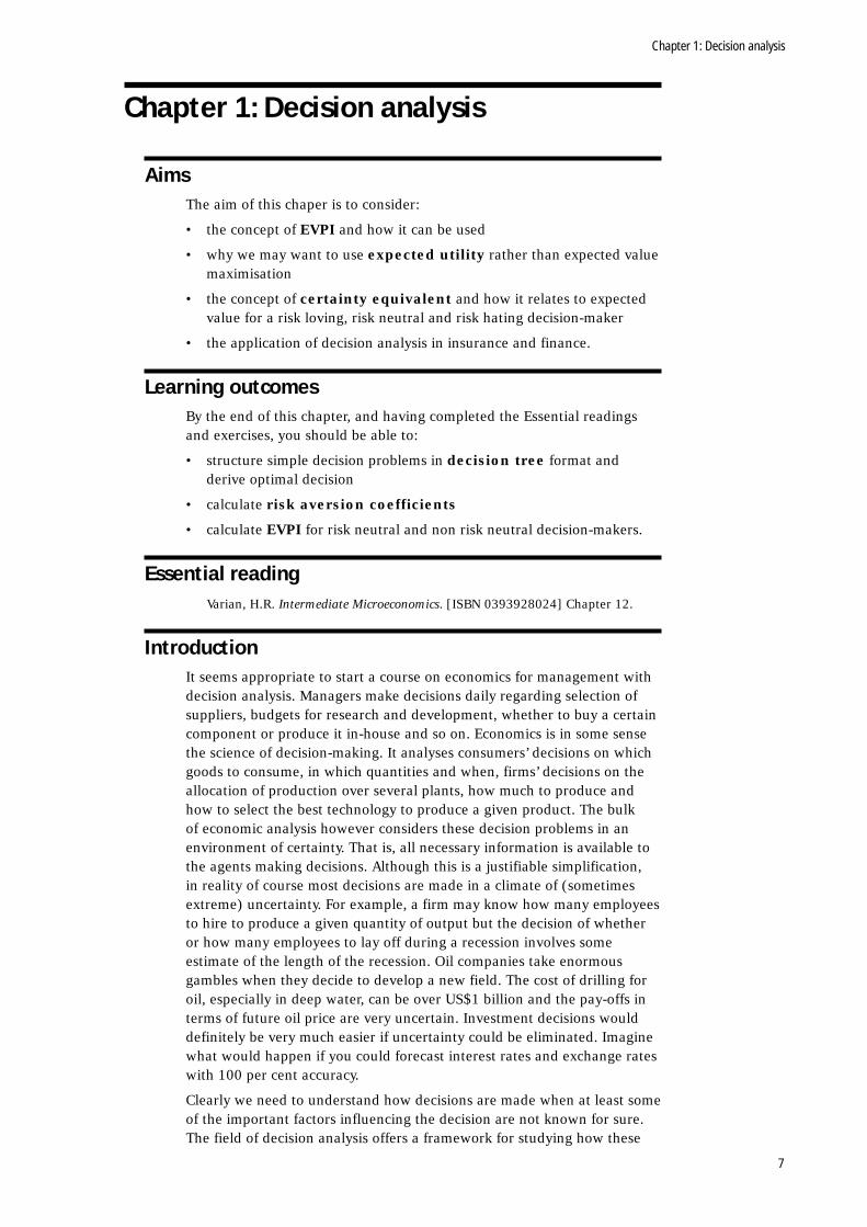
Cussoft Ltd., a firm which supplies customised software, must decide between two mutually exclusive contracts, one for the government and the other for a private firm. It is hard to estimate the costs Cussoft will incur under either contract but, from experience, it estimates that, if it contracts with a private firm, its profit will be £2 million, £0.7 million, or –£0.5 million with probabilities 0.25, 0.41 and 0.34 respectively. If it contracts with the government, its profit will be £4 million or –£2.5 million with respective probabilities 0.45 and 0.55. Which contract offers the greater expected profit?
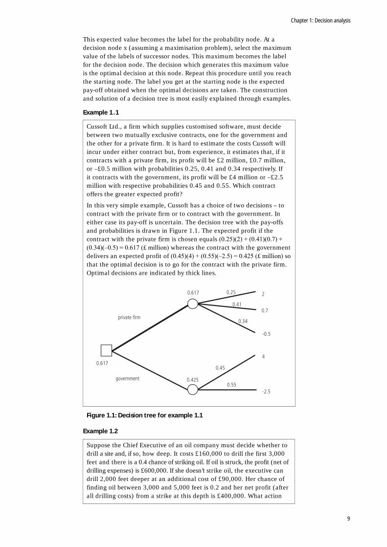
In this very simple example, Cussoft has a choice of two decisions – to contract with the private firm or to contract with the government. In either case its pay-off is uncertain. The decision tree with the pay-offs and probabilities is drawn in Figure 1.1. The expected profit if the contract with the private firm is chosen equals (0.25)(2) + (0.41)(0.7) + (0.34)(–0.5) = 0.617 (£ million) whereas the contract with the government delivers an expected profit of (0.45)(4) + (0.55)(–2.5) = 0.425 (£ million) so that the optimal decision is to go for the contract with the private firm. Optimal decisions are indicated by thick lines.
Figure 1.1: Decision tree for example 1.1
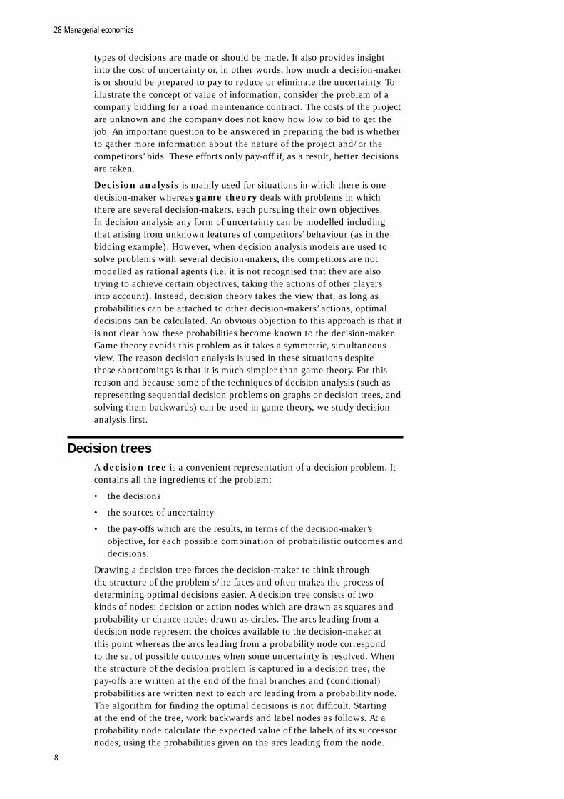
Example 1.2
Suppose the Chief Executive of an oil company must decide whether to drill a site and, if so, how deep. It costs £160,000 to drill the first 3,000 feet and there is a 0.4 chance of striking oil. If oil is struck, the profit (net of drilling expenses) is £600,000. If she doesn’t strike oil, the executive can drill 2,000 feet deeper at an additional cost of £90,000. Her chance of finding oil between 3,000 and 5,000 feet is 0.2 and her net profit (after all drilling costs) from a strike at this depth is £400,000. What action
private firm
government
0.617
0.4250.55
-2.5
-0.5
0.7
4
20.617
0.45
0.25
0.41
0.34
28 Managerial economics
10
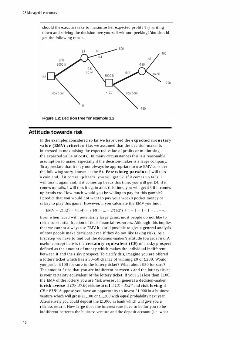
should the executive take to maximise her expected profit? Try writing down and solving the decision tree yourself without peeking! You should get the following result.
Figure 1.2: Decision tree for example 1.2
Attitude towards riskIn the examples considered so far we have used the expected monetary value (EMV) criterion (i.e. we assumed that the decision-maker is interested in maximising the expected value of profits or minimising the expected value of costs). In many circumstances this is a reasonable assumption to make, especially if the decision-maker is a large company. To appreciate that it may not always be appropriate to use EMV consider the following story, known as the St. Petersburg paradox. I will toss a coin and, if it comes up heads, you will get £2. If it comes up tails, I will toss it again and, if it comes up heads this time, you will get £4; if it comes up tails, I will toss it again and, this time, you will get £8 if it comes up heads etc. How much would you be willing to pay for this gamble? I predict that you would not want to pay your week’s pocket money or salary to play this game. However, if you calculate the EMV you find:
EMV = 2(1/2) + 4(1/4) + 8(l/8) + ... + 2n(1/2n) +... = 1 + l + 1 + .. . = ∞!
Even when faced with potentially large gains, most people do not like to risk a substantial fraction of their financial resources. Although this implies that we cannot always use EMV, it is still possible to give a general analysis of how people make decisions even if they do not like taking risks. As a first step we have to find out the decision-maker’s attitude towards risk. A useful concept here is the certainty equivalent (CE) of a risky prospect defined as the amount of money which makes the individual indifferent between it and the risky prospect. To clarify this, imagine you are offered a lottery ticket which has a 50–50 chance of winning £0 or £200. Would you prefer £100 for sure to the lottery ticket? What about £50 for sure? The amount £x so that you are indifferent between x and the lottery ticket is your certainty equivalent of the lottery ticket. If your x is less than £100, the EMV of the lottery, you are ‘risk averse’. In general a decision-maker is risk averse if CE < EMV, risk neutral if CE = EMV and risk loving if CE > EMV. Suppose you have an opportunity to invest £1,000 in a business venture which will gross £1,100 or £1,200 with equal probability next year. Alternatively you could deposit the £1,000 in bank which will give you a riskless return. How large does the interest rate have to be for you to be indifferent between the business venture and the deposit account (i.e. what
drill3000 ft
don’t drill
168
168
0
0.6no oil
oil
0.4
600
5000 ft
-120
-160
don’t drill
drill
-120
400
-250
no oil
oil
Chapter 1: Decision analysis
11
is your certainty equivalent? Are you a risk lover?)? Note that it is possible to be a risk lover for some lotteries and a risk hater for others.
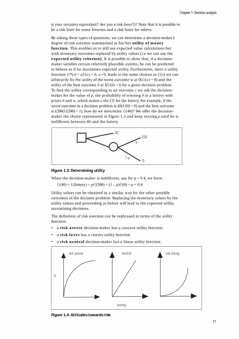
By asking these types of questions, we can determine a decision-maker’s degree of risk aversion summarised in his/her utility of money function. This enables us to still use expected value calculations but with monetary outcomes replaced by utility values (i.e we can use the expected utility criterion). It is possible to show that, if a decision-maker satisfies certain relatively plausible axioms, he can be predicted to behave as if he maximises expected utility. Furthermore, since a utility function U*(x) = aU(x) + b, a > 0, leads to the same choices as U(x) we can arbitrarily fix the utility of the worst outcome w at 0(U(w) = 0) and the utility of the best outcome b at l(U(b) = l) for a given decision problem. To find the utility corresponding to an outcome x we ask the decision-maker for the value of p, the probability of winning b in a lottery with prizes b and w, which makes x the CE for the lottery. For example, if the worst outcome in a decision problem is £0(U(0) = 0) and the best outcome is £200(U(200) = 1), how do we determine U(40)? We offer the decision-maker the choice represented in Figure 1.3 and keep varying p until he is indifferent between 40 and the lottery.
Figure 1.3: Determining utility
When the decision-maker is indifferent, say for p = 0.4, we have:
U(40) = U(lottery) = pU(200) + (1 – p)U(0) = p = 0.4.
Utility values can be obtained in a similar way for the other possible outcomes of the decision problem. Replacing the monetary values by the utility values and proceeding as before will lead to the expected utility maximising decisions.
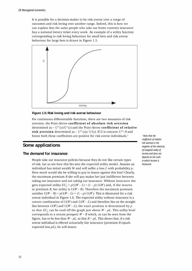
The definition of risk aversion can be rephrased in terms of the utility function:
• a risk averse decision-maker has a concave utility function
• a risk lover has a convex utility function
• a risk neutral decision-maker has a linear utility function.
Figure 1.4: Attitudes towards risk
40200
p
01-p
risk averse neutral risk loving
money
U
28 Managerial economics
12
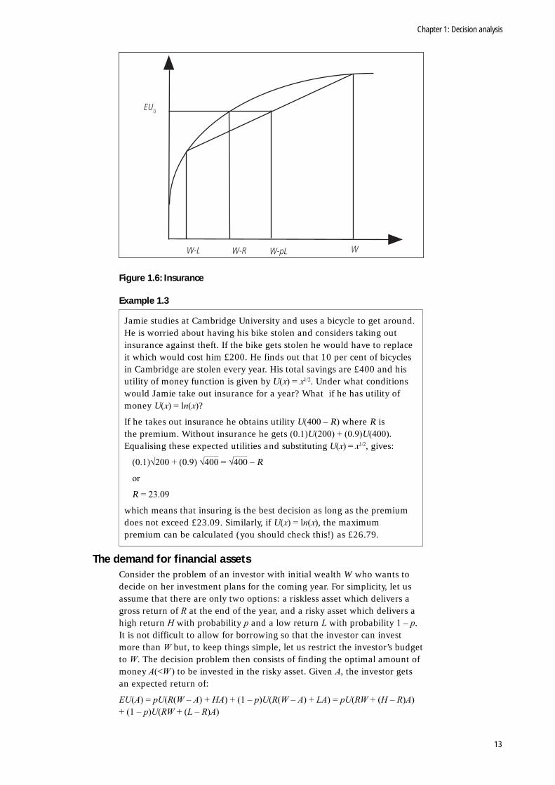
It is possible for a decision-maker to be risk averse over a range of outcomes and risk loving over another range. Indeed, this is how we can explain that the same people who take out home contents insurance buy a national lottery ticket every week. An example of a utility function corresponding to risk loving behaviour for small bets and risk averse behaviour for large bets is drawn in Figure 1.5.
Figure 1.5: Risk loving and risk averse behaviour
For continuous differentiable functions, there are two measures of risk aversion, the Pratt-Arrow coefficient of absolute risk aversion determined as – U'' (x)/U' (x) and the Pratt-Arrow coefficient of relative risk aversion determined as – U′′ (x)x/ U'(x). If U is concave U′′< 0 and hence both these coefficients are positive for risk averse individuals.1
Some applications
The demand for insurance
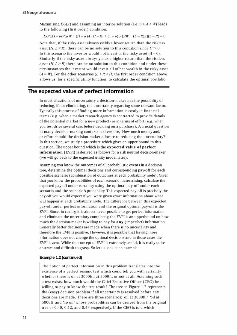
People take out insurance policies because they do not like certain types of risk. Let us see how this fits into the expected utility model. Assume an individual has initial wealth W and will suffer a loss L with probability p. How much would she be willing to pay to insure against this loss? Clearly, the maximum premium R she will pay makes her just indifferent between taking out insurance and not taking out insurance. Without insurance she gets expected utility EU0 = pU(W – L) + (1 – p) U(W ) and, if she insures at premium R, her utility is U(W – R). Therefore the maximum premium satisfies U(W – R) = pU(W – L) + (1 – p) U(W ). This is illustrated for a risk averse individual in Figure 1.6. The expected utility without insurance is a convex combination of U(W ) and U(W – L) and therefore lies on the straight line between U(W ) and U(W – L); the exact position is determined by p so that EU0 can be read off the graph just above W – pL. This utility level corresponds to a certain prospect W – R which, as can be seen from the figure, has to be less than W – pL, so that R > pL. This shows that, if a risk averse individual is offered actuarially fair insurance (premium R equals expected loss pL), he will insure.
money
U
1 Note that the coeffi cient of relative risk aversion is the negative of the elasticity of marginal utility of income and does not depend on the units in which income is measured.
Chapter 1: Decision analysis
13
EU0
W-L W-R W-pL W
Figure 1.6: Insurance
Example 1.3
Jamie studies at Cambridge University and uses a bicycle to get around. He is worried about having his bike stolen and considers taking out insurance against theft. If the bike gets stolen he would have to replace it which would cost him £200. He finds out that 10 per cent of bicycles in Cambridge are stolen every year. His total savings are £400 and his utility of money function is given by U(x) = x1/2. Under what conditions would Jamie take out insurance for a year? What if he has utility of money U(x) = ln(x)?
If he takes out insurance he obtains utility U(400 – R) where R is the premium. Without insurance he gets (0.1)U(200) + (0.9)U(400). Equalising these expected utilities and substituting U(x) = x1/2, gives:
(0.1)√200 + (0.9) √400 = √400 – R
or
R = 23.09
which means that insuring is the best decision as long as the premium does not exceed £23.09. Similarly, if U(x) = ln(x), the maximum premium can be calculated (you should check this!) as £26.79.
The demand for financial assetsConsider the problem of an investor with initial wealth W who wants to decide on her investment plans for the coming year. For simplicity, let us assume that there are only two options: a riskless asset which delivers a gross return of R at the end of the year, and a risky asset which delivers a high return H with probability p and a low return L with probability 1 – p. It is not difficult to allow for borrowing so that the investor can invest more than W but, to keep things simple, let us restrict the investor’s budget to W. The decision problem then consists of finding the optimal amount of money A(<W ) to be invested in the risky asset. Given A, the investor gets an expected return of:
EU(A) = pU(R(W – A) + HA) + (1 – p)U(R(W – A) + LA) = pU(RW + (H – R)A) + (1 – p)U(RW + (L – R)A)
28 Managerial economics
14
Maximising EU(A) and assuming an interior solution (i.e. 0 < A < W) leads to the following (first order) condition:
EU'(A) = pU'(RW + (H – R)A)(H – R) + (1 – p)U'(RW + (L – R)A)(L – R) = 0
Note that, if the risky asset always yields a lower return than the riskless asset (H, L < R), there can be no solution to this condition since U' > 0. In this scenario the investor would not invest in the risky asset (A = 0). Similarly, if the risky asset always yields a higher return than the riskless asset (H, L > R) there can be no solution to this condition and under these circumstances the investor would invest all of her wealth in the risky asset (A = W). For the other scenarios (L < R < H) the first order condition above allows us, for a specific utility function, to calculate the optimal portfolio.
The expected value of perfect information
In most situations of uncertainty a decision-maker has the possibility of reducing, if not eliminating, the uncertainty regarding some relevant factor. Typically this process of finding more information is costly in financial terms (e.g. when a market research agency is contracted to provide details of the potential market for a new product) or in terms of effort (e.g. when you test drive several cars before deciding on a purchase). A crucial question in many decision-making contexts is therefore, ‘How much money and/ or effort should the decision-maker allocate to reducing the uncertainty?’ In this section, we study a procedure which gives an upper bound to this question. The upper bound which is the expected value of perfect information (EVPI) is derived as follows for a risk neutral decision-maker (we will go back to the expected utility model later).
Assuming you know the outcomes of all probabilistic events in a decision tree, determine the optimal decisions and corresponding pay-off for each possible scenario (combination of outcomes at each probability node). Given that you know the probabilities of each scenario materialising, calculate the expected pay-off under certainty using the optimal pay-off under each scenario and the scenario’s probability. This expected pay-off is precisely the pay-off you would expect if you were given exact information about what will happen at each probability node. The difference between this expected pay-off under perfect information and the original optimal pay-off is the EVPI. Since, in reality, it is almost never possible to get perfect information and eliminate the uncertainty completely, the EVPI is an upperbound on how much the decision-maker is willing to pay for any (imperfect) information. Generally better decisions are made when there is no uncertainty and therefore the EVPI is positive. However, it is possible that having more information does not change the optimal decisions and in those cases the EVPI is zero. While the concept of EVPI is extremely useful, it is really quite abstract and difficult to grasp. So let us look at an example.
Example 1.2 (continued)
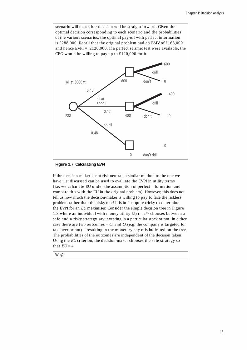
The notion of perfect information in this problem translates into the existence of a perfect seismic test which could tell you with certainty whether there is oil at 3000ft., at 5000ft. or not at all. Assuming such a test exists, how much would the Chief Executive Officer (CEO) be willing to pay to know the test result? The tree in Figure 1.7 represents the (easy) decision problem if all uncertainty is resolved before any decisions are made. There are three scenarios: ‘oil at 3000ft.’, ‘oil at 5000ft’ and ‘no oil’ whose probabilities can be derived from the original tree as 0.40, 0.12, and 0.48 respectively. If the CEO is told which
Chapter 1: Decision analysis
15
scenario will occur, her decision will be straightforward. Given the optimal decision corresponding to each scenario and the probabilities of the various scenarios, the optimal pay-off with perfect information is £288,000. Recall that the original problem had an EMV of £168,000 and hence EVPI = £120,000. If a perfect seismic test were available, the CEO would be willing to pay up to £120,000 for it.
Figure 1.7: Calculating EVPI
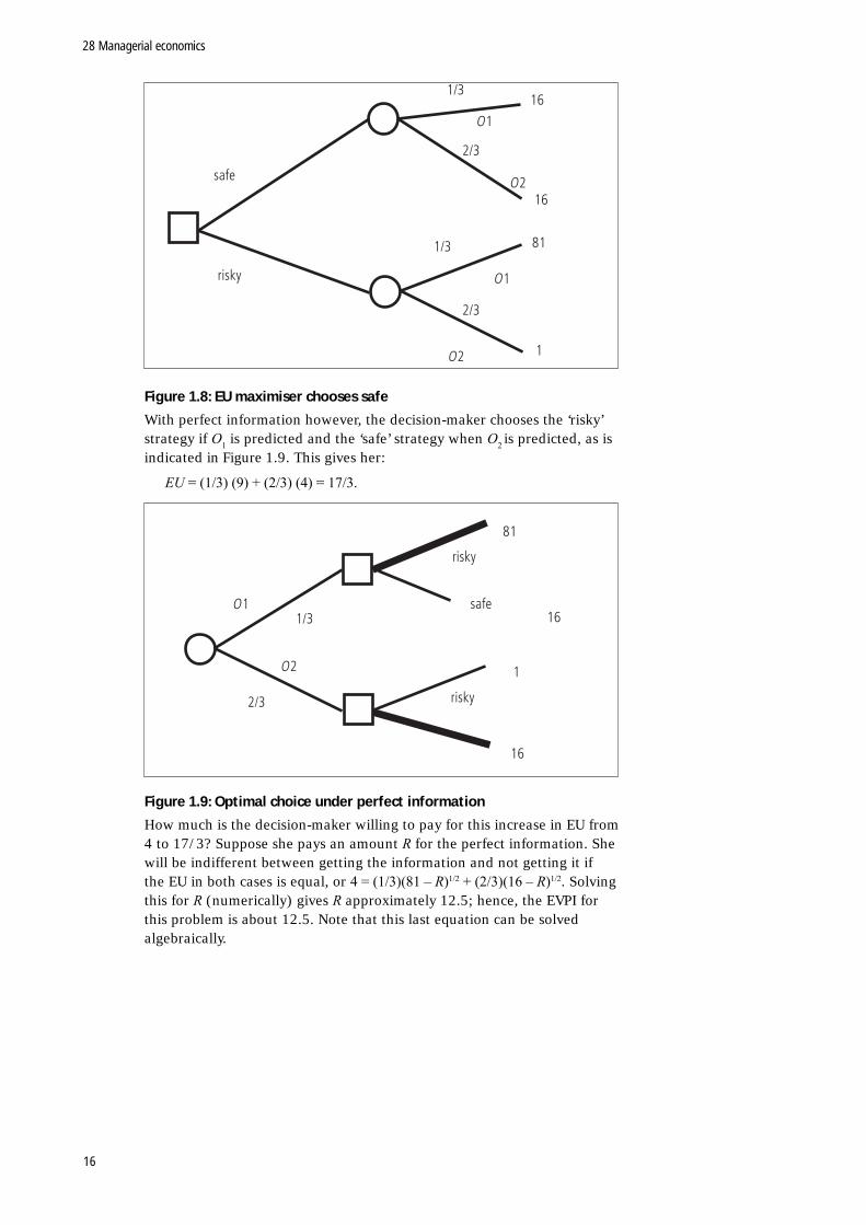
If the decision-maker is not risk neutral, a similar method to the one we have just discussed can be used to evaluate the EVPI in utility terms (i.e. we calculate EU under the assumption of perfect information and compare this with the EU in the original problem). However, this does not tell us how much the decision-maker is willing to pay to face the riskless problem rather than the risky one! It is in fact quite tricky to determine the EVPI for an EU maximiser. Consider the simple decision tree in Figure 1.8 where an individual with money utility U(x) = x 1/2 chooses between a safe and a risky strategy, say investing in a particular stock or not. In either case there are two outcomes – O1 and O2 (e.g. the company is targeted for takeover or not) – resulting in the monetary pay-offs indicated on the tree. The probabilities of the outcomes are independent of the decision taken. Using the EU criterion, the decision-maker chooses the safe strategy so that EU = 4.
Why?
oil at 3000 ft
don’t drill
oil at5000 ft
no oil
drill
don’t
0.40
0.48
288
600
600
400
400
0.12
drill
don’t
0
0
0
0
28 Managerial economics
16
Figure 1.8: EU maximiser chooses safe
With perfect information however, the decision-maker chooses the ‘risky’ strategy if O1 is predicted and the ‘safe’ strategy when O2 is predicted, as is indicated in Figure 1.9. This gives her:
EU = (1/3) (9) + (2/3) (4) = 17/3.
Figure 1.9: Optimal choice under perfect information
How much is the decision-maker willing to pay for this increase in EU from 4 to 17/3? Suppose she pays an amount R for the perfect information. She will be indifferent between getting the information and not getting it if the EU in both cases is equal, or 4 = (1/3)(81 – R)1/2 + (2/3)(16 – R)1/2. Solving this for R (numerically) gives R approximately 12.5; hence, the EVPI for this problem is about 12.5. Note that this last equation can be solved algebraically.
safe
risky
1/3
2/3
1/3
2/3
O1
O2
O2
O1
16
16
81
1
risky
risky
safeO1
O2
2/3
1/3
81
16
16
1
Chapter 1: Decision analysis
17
A reminder of your learning outcomesHaving completed this chapter, and the Essential readings and exercises, you should be able to:
• structure simple decision problems in decision tree format and derive optimal decision
• calculate risk aversion coefficients
• calculate EVPI for risk neutral and non risk neutral decision-makers.
Sample exercises1. London Underground (LU) is facing a courtcase by legal firm Snook&Co,
representing the family of Mr Addams who was killed in the Kings Cross fire. LU has estimated the damages it will have to pay if the case goes to court as follows: £1,000,000, £600,000 or £0 with probabilities 0.2, 0.5 and 0.3 respectively. Its legal expenses are estimated at £100,000 in addition to these awards. The alternative to allowing the case to go to court is for LU to enter into out-of-court settlement negotiations. It is uncertain about the amount of money Snook&Co. are prepared to settle for. They may only wish to settle for a high amount (£900,000) or they may be willing to settle for a reasonable amount (£400,000). Each scenario is equally likely. If they are willing to settle for £400,000 they will of course accept an offer of £900,000. On the other hand, if they will only settle for £900,000 they will reject an offer of £400,000. LU, if it decides to enter into negotiations, will offer £400,000 or £900,000 to Snook & Co. who will either accept (and waive any future right to sue) or reject and take the case to court. The legal cost of pursuing a settlement whether or not one is reached is £50,000. Determine the strategy which minimises LU’s expected total cost.
2. Rickie is considering setting up a business in the field of entertainment at children’s parties. He estimates that he would earn a gross revenue of £9,000 or £4,000 with a 50–50 chance. His initial wealth is zero. What is the largest value of the cost which would make him start this business:
a. if his utility of money function is U(x) = ax + b where a > 0
b. if U(x) = x1/2; for x > 0 and U(x) = –(–x)1/2 for x < 0
c. if U(x) = x2, for x > 0 and U(x) = –x2 for x < 0.
3. Find the coefficient of absolute risk aversion for U(x) = a – b.exp(–cx) and the coefficient of relative risk aversion for U(x) = a + b.ln(x).
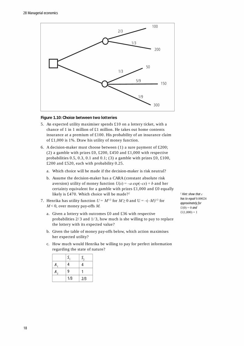
4. Find a volunteer (preferably someone who doesn’t know expected utility theory) and estimate their utility of money function to predict their choice between the two lotteries below. Pay-offs are given in monetary value (£). Check your prediction.
28 Managerial economics
18
Figure 1.10: Choice between two lotteries
5. An expected utility maximiser spends £10 on a lottery ticket, with a chance of 1 in 1 million of £1 million. He takes out home contents insurance at a premium of £100. His probability of an insurance claim of £1,000 is 1%. Draw his utility of money function.
6. A decision-maker must choose between (1) a sure payment of £200; (2) a gamble with prizes £0, £200, £450 and £1,000 with respective probabilities 0.5, 0.3, 0.1 and 0.1; (3) a gamble with prizes £0, £100, £200 and £520, each with probability 0.25.
a. Which choice will be made if the decision-maker is risk neutral?
b. Assume the decision-maker has a CARA (constant absolute risk aversion) utility of money function U(x) = –a exp(–cx) + b and her certainty equivalent for a gamble with prizes £1,000 and £0 equally likely is £470. Which choice will be made?2
7. Henrika has utility function U = M 1/2 for M ≥ 0 and U = –(–M )1/2 for M < 0, over money pay-offs M.
a. Given a lottery with outcomes £0 and £36 with respective probabilities 2/3 and 1/3, how much is she willing to pay to replace the lottery with its expected value?
b. Given the table of money pay-offs below, which action maximises her expected utility?
c. How much would Henrika be willing to pay for perfect information regarding the state of nature?
S1 S2
A14 4
A29 1
1/3 2/3
2/3
1/3
1/3
1/9
5/9
100
200
50
150
300
2 Hint: show that c has to equal 0.00024 approximately for U(0) = 0 and U(1,000) = 1
Chapter 2: Game theory
19
Chapter 2: Game theory
AimsThe aim of this chaper is to consider:
• the concept of information set and why it is not needed in decision analysis
• why it is useful to have both extensive form and normal form representations of a game
• the importance of the prisoners’ dilemma as a paradigm for many social interactions
• the concept of dominated strategies and the rationale for eliminating them in analysis of a game
• the concept of Nash equilibrium (this is absolutely essential!)
• the concept of non-credible threats and its application in entry deterrence.
Learning outcomesBy the end of this chapter, and having completed the Essential readings and exercises, you should be able to:
• represent a simple multi-person decision problem using a game tree
• translate from an extensive form representation to the normal form representation
• find Nash equilibria in pure and mixed strategies
• explain why in a finitely repeated prisoners’ dilemma game cheating is a Nash equilibrium
• explain the chainstore paradox.
Essential readingsTirole, J. The Theory of Industrial Organization. Chapter 11.Varian, H.R. Intermediate Microeconomics. Chapters 28 and 29.
Further readingAxelrod, R. The evolution of cooperation. (New York, Basic Books 1984)
[ISBN 0465021212].Kreps, D. and R. Wilson ‘Reputation and imperfect information’, Journal of
economic theory (1982) 27, pp.253–79.Milgrom, P. and J. Roberts ‘Predation, reputation and entry deterrence’, Journal
of economic theory (1982) 27, pp.280–312.‘Mumbo-jumbo, Super-jumbo’, The Economist, 12 June 1993, p.83Nash, J. ‘Noncooperative games’, Annals of Mathematics 54 1951, pp.289–95.‘Now for the really big one’, The Economist, 9 January 1993, p.83.‘Plane wars’, The Economist, 11 June 1994, pp.61–62.Selton, R. ‘ The chain store paradox’, Theory and Decision (9) 1978, pp.127–59.‘The flying monopolists’, The Economist, 19 June 1993, p.18.
28 Managerial economics
20
IntroductionGame theory extends the theory of individual decision-making to situations of strategic interdependence: that is, situations where players (decision-makers) take other players’ behaviour into account when making their decisions. The pay-offs resulting from any decision (and possibly random events) are generally dependent on others’ actions.
A distinction is made between cooperative game theory and noncooperative game theory. In cooperative games, coalitions or groups of players are analysed. Players can communicate and make binding agreements. The theory of noncooperative games assumes that no such agreements are possible. Each player in choosing his or her actions, subject to the rules of the game, is motivated by self-interest. Because of the larger scope for application of noncooperative games to managerial economics, we will limit our discussion to noncooperative games.
To model an economic situation as a game involves translating the essential characteristics of the situation into rules of a game. The following must be determined:
• the number of players
• their possible actions at every point in time
• the pay-offs for all possible combinations of moves by the players
• the information structure (what do players know when they have to make their decisions?).
All this information can be presented in a game tree which is the game theory equivalent of the decision tree. This way of describing the game is called the extensive form representation.
It is often convenient to think of players’ behaviour in a game in terms of strategies. A strategy tells you what the player will do each time s/he has to make a decision. So, if you know the player’s strategy, you can predict his behaviour in all possible scenarios with respect to the other players’ behaviour. When you list or describe the strategies available to each player and attach pay-offs to all possible combinations of strategies by the players, the resulting ‘summary’ of the game is called a normal form or strategic form representation.
In games of complete information all players know the rules of the game. In incomplete information games at least one player only has probabilistic information about some elements of the game (e.g. the other players’ precise characteristics). An example of the latter category is a game involving an insurer – who only has probabilistic information about the carelessness of an individual who insures his car against theft – and the insured individual who knows how careless he is. A firm is also likely to know more about its own costs than about its competitors’ costs. In games of perfect information all players know the earlier moves made by themselves and by the other players. In games of perfect recall players remember their own moves and do not forget any information which they obtained in the course of game play. They do not necessarily learn about other players’ moves.
Game theory, as decision theory, assumes rational decision-makers. This means that players are assumed to make decisions or choose strategies which will give them the highest possible expected pay-off (or utility). Each player also knows that other players are rational and that they know that he knows they are rational and so on. In a strategic situation the question arises whether it could not be in an individual player’s interest to convince the other players that he is irrational. (This is a complicated issue which we will consider in
Chapter 2: Game theory
21
the later sections of this chapter. All I want to say for now is that ultimately the creation of an impression of irrationality may be a rational decision.)
Before we start our study of game theory, a ‘health warning’ may be appropriate. It is not realistic to expect that you will be able to use game theory as a technique for solving real problems. Most realistic situations are too complex to analyse from a game theoretical perspective. Furthermore, game theory does not offer any optimal solutions or solution procedures for most practical problems. However, through a study of game theory, insights can be obtained which would be difficult to obtain in another way and game theoretic modelling helps decision-makers think through all aspects of the strategic problems they are facing. As is true of mathematical models in general it allows you to check intuitive answers for logical consistency.
Extensive form gamesAs mentioned above, the extensive form representation of a game is similar to a decision tree. The order of play and the possible decisions at each decision point for each player are indicated as well as the information structure, the outcomes or pay-offs and probabilities. As in decision analysis the pay-offs are not always financial. They may reflect the player’s utility of reaching a given outcome. A major difference with decision analysis is that in analysing games and in constructing the game tree, the notion of information set is important. When there is only one decision-maker, the decision-maker has perfect knowledge of her own earlier choices. In a game, the players often have to make choices not knowing which decisions have been taken or are taken at the same time by the other players. To indicate that a player does not know her position in the tree exactly, the possible locations are grouped or linked in an information set, Since a player should not be able to deduce from the nature or number of alternative choices available to her where she is in the information set, her set of possible actions has to be identical at every node in the information set. For the same reason, if two nodes are in the same information set, the same player has to make a decision at these nodes. In games of perfect information the players know all the moves made at any stage of the game and therefore all information sets consist of single nodes.
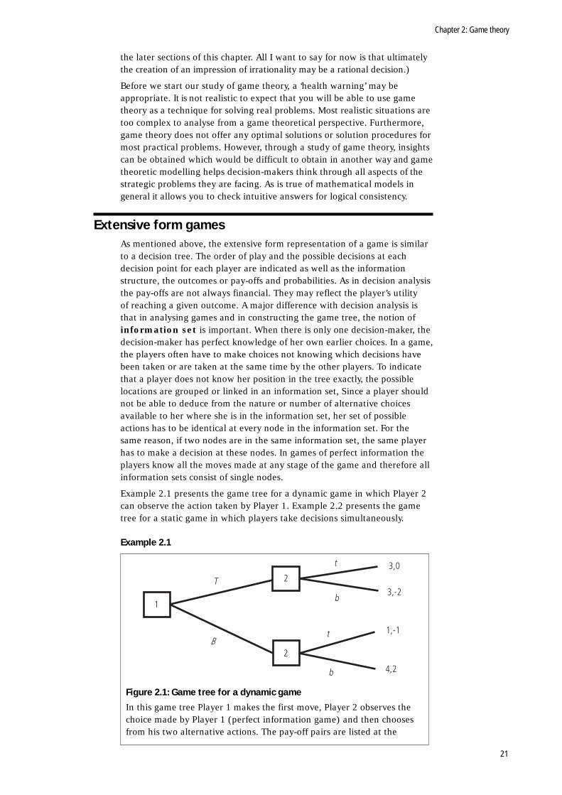
Example 2.1 presents the game tree for a dynamic game in which Player 2 can observe the action taken by Player 1. Example 2.2 presents the game tree for a static game in which players take decisions simultaneously.
Example 2.1
Figure 2.1: Game tree for a dynamic game
In this game tree Player 1 makes the first move, Player 2 observes the choice made by Player 1 (perfect information game) and then chooses from his two alternative actions. The pay-off pairs are listed at the
1
2
2
T
B
b
b
t
t 3,0
3,-2
1,-1
4,2
28 Managerial economics
22
endpoints of the tree. For example, when Player 1 chooses B and Player 2 chooses t, they receive pay-offs of 1 and –1 respectively. Games of perfect information are easy to analyse. As in decision analysis, we can just start at the end of the tree and work backwards (Kuhn’s algorithm). When Player 2 is about to move and he is at the top node, he chooses t since this gives him a pay-off of 0 rather than –2 corresponding to b. When he is at the bottom node, he gets a pay-off of 2 by choosing b. Player 1 knows the game tree and can anticipate these choices of Player 2. He therefore anticipates a pay-off of 3 if he chooses T and 4 if he chooses B. We can conclude that Player 1 will take action B and Player 2 will take action b.
Let us use this example to explain what is meant by a strategy. Player 1 has two strategies: T and B. (Remember that a strategy should state what the player will do in each eventuality.) For Player 2 therefore, each strategy consists of a pair of actions, one to take if he ends up at the top node and one to take if he ends up at the bottom node. Player 2 has four possible strategies, namely:
• (t if T, t if B)
• (t if T, b if B)
• (b if T, t if B)
• (b if T, b if B)
• or {(t, t), (t, b), (b, t),(b, b)} for short.
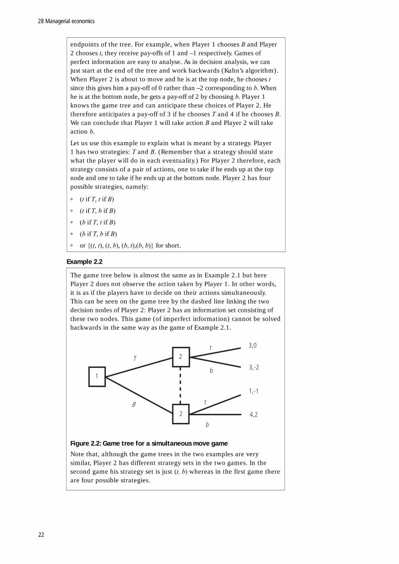
Example 2.2
The game tree below is almost the same as in Example 2.1 but here Player 2 does not observe the action taken by Player 1. In other words, it is as if the players have to decide on their actions simultaneously. This can be seen on the game tree by the dashed line linking the two decision nodes of Player 2: Player 2 has an information set consisting of these two nodes. This game (of imperfect information) cannot be solved backwards in the same way as the game of Example 2.1.
Figure 2.2: Game tree for a simultaneous move game
Note that, although the game trees in the two examples are very similar, Player 2 has different strategy sets in the two games. In the second game his strategy set is just (t, b) whereas in the first game there are four possible strategies.
1
2
2
T
B
b
b
t
t 3,0
3,-2
1,-1
4,2
Chapter 2: Game theory
23
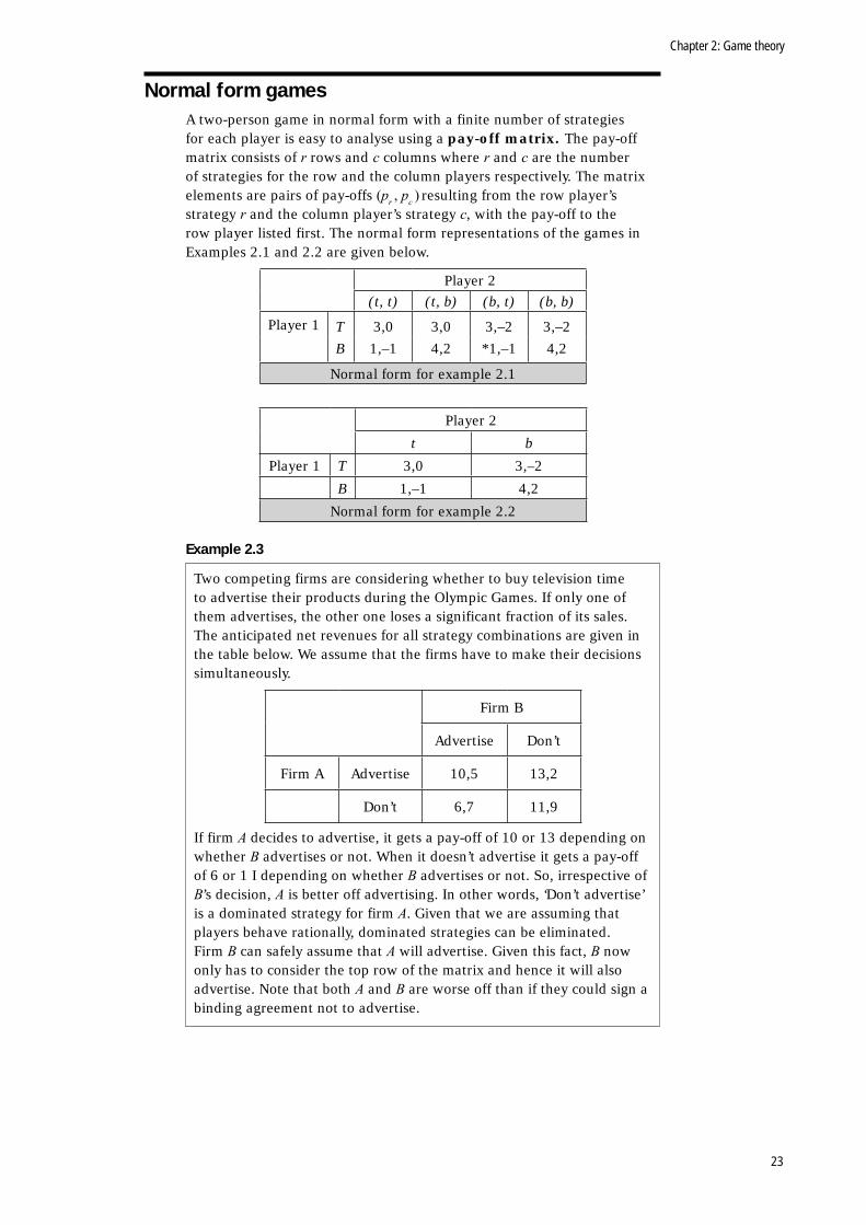
Normal form gamesA two-person game in normal form with a finite number of strategies for each player is easy to analyse using a pay-off matrix. The pay-off matrix consists of r rows and c columns where r and c are the number of strategies for the row and the column players respectively. The matrix elements are pairs of pay-offs (pr , pc ) resulting from the row player’s strategy r and the column player’s strategy c, with the pay-off to the row player listed first. The normal form representations of the games in Examples 2.1 and 2.2 are given below.
Player 2(t, t) (t, b) (b, t) (b, b)
Player 1 TB
3,0
1,–1
3,0
4,2
3,–2
*1,–1
3,–2
4,2
Normal form for example 2.1
Player 2
t b
Player 1 T 3,0 3,–2
B 1,–1 4,2
Normal form for example 2.2
Example 2.3
Two competing firms are considering whether to buy television time to advertise their products during the Olympic Games. If only one of them advertises, the other one loses a significant fraction of its sales. The anticipated net revenues for all strategy combinations are given in the table below. We assume that the firms have to make their decisions simultaneously.
Firm B
Advertise Don’t
Firm A Advertise 10,5 13,2
Don’t 6,7 11,9
If firm A decides to advertise, it gets a pay-off of 10 or 13 depending on whether B advertises or not. When it doesn’t advertise it gets a pay-off of 6 or 1 I depending on whether B advertises or not. So, irrespective of B’s decision, A is better off advertising. In other words, ‘Don’t advertise’ is a dominated strategy for firm A. Given that we are assuming that players behave rationally, dominated strategies can be eliminated. Firm B can safely assume that A will advertise. Given this fact, B now only has to consider the top row of the matrix and hence it will also advertise. Note that both A and B are worse off than if they could sign a binding agreement not to advertise.
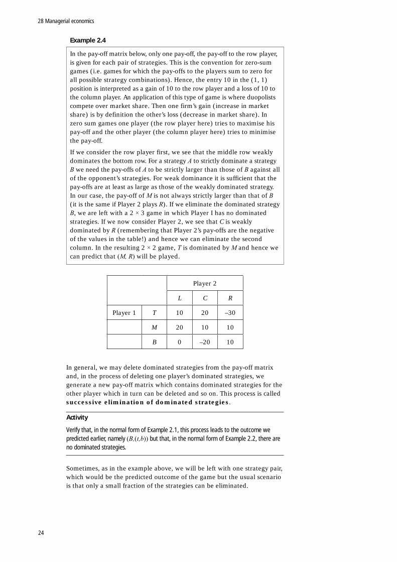
28 Managerial economics
24
Example 2.4
In the pay-off matrix below, only one pay-off, the pay-off to the row player, is given for each pair of strategies. This is the convention for zero-sum games (i.e. games for which the pay-offs to the players sum to zero for all possible strategy combinations). Hence, the entry 10 in the (1, 1) position is interpreted as a gain of 10 to the row player and a loss of 10 to the column player. An application of this type of game is where duopolists compete over market share. Then one firm’s gain (increase in market share) is by definition the other’s loss (decrease in market share). In zero sum games one player (the row player here) tries to maximise his pay-off and the other player (the column player here) tries to minimise the pay-off.
If we consider the row player first, we see that the middle row weakly dominates the bottom row. For a strategy A to strictly dominate a strategy B we need the pay-offs of A to be strictly larger than those of B against all of the opponent’s strategies. For weak dominance it is sufficient that the pay-offs are at least as large as those of the weakly dominated strategy. In our case, the pay-off of M is not always strictly larger than that of B (it is the same if Player 2 plays R). If we eliminate the dominated strategy B, we are left with a 2 × 3 game in which Player I has no dominated strategies. If we now consider Player 2, we see that C is weakly dominated by R (remembering that Player 2’s pay-offs are the negative of the values in the table!) and hence we can eliminate the second column. In the resulting 2 × 2 game, T is dominated by M and hence we can predict that (M, R) will be played.
Player 2
L C R
Player 1 T 10 20 –30
M 20 10 10
B 0 –20 10
In general, we may delete dominated strategies from the pay-off matrix and, in the process of deleting one player’s dominated strategies, we generate a new pay-off matrix which contains dominated strategies for the other player which in turn can be deleted and so on. This process is called successive elimination of dominated strategies.
Activity
Verify that, in the normal form of Example 2.1, this process leads to the outcome we predicted earlier, namely (B,(t,b)) but that, in the normal form of Example 2.2, there are no dominated strategies.
Sometimes, as in the example above, we will be left with one strategy pair, which would be the predicted outcome of the game but the usual scenario is that only a small fraction of the strategies can be eliminated.
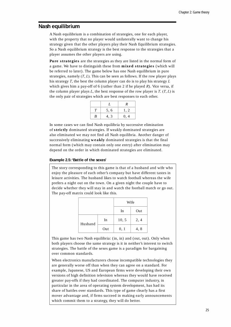
Chapter 2: Game theory
25
Nash equilibriumA Nash equilibrium is a combination of strategies, one for each player, with the property that no player would unilaterally want to change his strategy given that the other players play their Nash Equilibrium strategies. So a Nash equilibrium strategy is the best response to the strategies that a player assumes the other players are using.
Pure strategies are the strategies as they are listed in the normal form of a game. We have to distinguish these from mixed strategies (which will be referred to later). The game below has one Nash equilibrium in pure strategies, namely (T, L). This can be seen as follows. If the row player plays his strategy T, the best the column player can do is to play his strategy L which gives him a pay-off of 6 (rather than 2 if he played R). Vice versa, if the column player plays L, the best response of the row player is T. (T, L) is the only pair of strategies which are best responses to each other.
L R
T 5, 6 1, 2
B 4, 3 0, 4
In some cases we can find Nash equilibria by successive elimination of strictly dominated strategies. If weakly dominated strategies are also eliminated we may not find all Nash equilibria. Another danger of successively eliminating weakly dominated strategies is that the final normal form (which may contain only one entry) after elimination may depend on the order in which dominated strategies are eliminated.
Example 2.5: ‘Battle of the sexes’
The story corresponding to this game is that of a husband and wife who enjoy the pleasure of each other’s company but have different tastes in leisure activities. The husband likes to watch football whereas the wife prefers a night out on the town. On a given night the couple have to decide whether they will stay in and watch the football match or go out. The pay-off matrix could look like this.
Wife
In Out
HusbandIn 10, 5 2, 4
Out 0, 1 4, 8
This game has two Nash equilibria: (in, in) and (out, out). Only when both players choose the same strategy is it in neither’s interest to switch strategies. The battle of the sexes game is a paradigm for bargaining over common standards.
When electronics manufacturers choose incompatible technologies they are generally worse off than when they can agree on a standard. For example, Japanese, US and European firms were developing their own versions of high definition television whereas they would have received greater pay-offs if they had coordinated. The computer industry, in particular in the area of operating system development, has had its share of battles over standards. This type of game clearly has a first mover advantage and, if firms succeed in making early announcements which commit them to a strategy, they will do better.
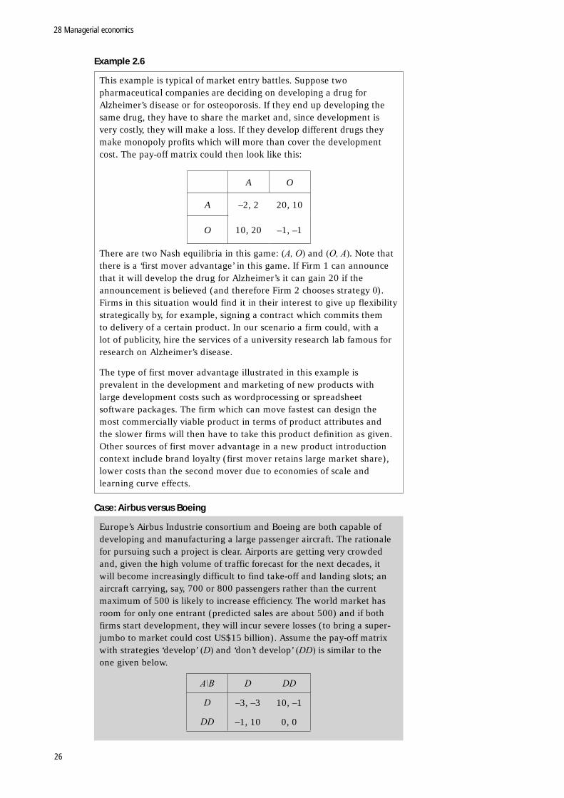
28 Managerial economics
26
Example 2.6
This example is typical of market entry battles. Suppose two pharmaceutical companies are deciding on developing a drug for Alzheimer’s disease or for osteoporosis. If they end up developing the same drug, they have to share the market and, since development is very costly, they will make a loss. If they develop different drugs they make monopoly profits which will more than cover the development cost. The pay-off matrix could then look like this:
A O
A –2, 2 20, 10
O 10, 20 –1, –1
There are two Nash equilibria in this game: (A, O) and (O, A). Note that there is a ‘first mover advantage’ in this game. If Firm 1 can announce that it will develop the drug for Alzheimer’s it can gain 20 if the announcement is believed (and therefore Firm 2 chooses strategy 0). Firms in this situation would find it in their interest to give up flexibility strategically by, for example, signing a contract which commits them to delivery of a certain product. In our scenario a firm could, with a lot of publicity, hire the services of a university research lab famous for research on Alzheimer’s disease.
The type of first mover advantage illustrated in this example is prevalent in the development and marketing of new products with large development costs such as wordprocessing or spreadsheet software packages. The firm which can move fastest can design the most commercially viable product in terms of product attributes and the slower firms will then have to take this product definition as given. Other sources of first mover advantage in a new product introduction context include brand loyalty (first mover retains large market share), lower costs than the second mover due to economies of scale and learning curve effects.
Case: Airbus versus Boeing
Europe’s Airbus Industrie consortium and Boeing are both capable of developing and manufacturing a large passenger aircraft. The rationale for pursuing such a project is clear. Airports are getting very crowded and, given the high volume of traffic forecast for the next decades, it will become increasingly difficult to find take-off and landing slots; an aircraft carrying, say, 700 or 800 passengers rather than the current maximum of 500 is likely to increase efficiency. The world market has room for only one entrant (predicted sales are about 500) and if both firms start development, they will incur severe losses (to bring a super-jumbo to market could cost US$15 billion). Assume the pay-off matrix with strategies ‘develop’ (D) and ‘don’t develop’ (DD) is similar to the one given below.
A\B D DD
D –3, –3 10, –1
DD –1, 10 0, 0
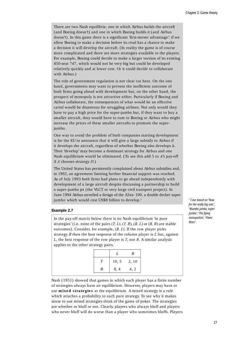
Chapter 2: Game theory
27
There are two Nash equilibria: one in which Airbus builds the aircraft (and Boeing doesn’t) and one in which Boeing builds it (and Airbus doesn’t). In this game there is a significant ‘first-mover advantage’: if we allow Boeing to make a decision before its rival has a chance to make a decision it will develop the aircraft. (In reality the game is of course more complicated and there are more strategies available to the players. For example, Boeing could decide to make a larger version of its existing 450-seat 747, which would not be very big but could be developed relatively quickly and at lower cost. Or it could decide to collaborate with Airbus.)
The role of government regulation is not clear cut here. On the one hand, governments may want to prevent the inefficient outcome of both firms going ahead with development but, on the other hand, the prospect of monopoly is not attractive either. Particularly if Boeing and Airbus collaborate, the consequences of what would be an effective cartel would be disastrous for struggling airlines. Not only would they have to pay a high price for the super-jumbo but, if they want to buy a smaller aircraft, they would have to rum to Boeing or Airbus who might increase the prices of these smaller aircrafts to promote the super-jumbo.
One way to avoid the problem of both companies starting development is for the EU to announce that it will give a large subsidy to Airbus if it develops the aircraft, regardless of whether Boeing also develops it. Then ‘develop’ may become a dominant strategy for Airbus and one Nash equilibrium would be eliminated. (To see this add 5 to A’s pay-off if A chooses strategy D.)
The United States has persistently complained about Airbus subsidies and, in 1992, an agreement limiting further financial support was reached. As of July 1993 both firms had plans to go ahead independently with development of a large aircraft despite discussing a partnership to build a super-jumbo jet (the VLCT or very large civil transport project). In June 1994 Airbus unveiled a design of the A3xx- 100, a double decker super jumbo which would cost US$8 billion to develop.1
Example 2.7
In the pay-off matrix below there is no Nash equilibrium ‘in pure strategies’ (i.e. none of the pairs (T, L), (T, R), (B, L) or (B, R) are stable outcomes). Consider, for example, (B, L). If the row player picks strategy B then the best response of the column player is L but, against L, the best response of the row player is T, not B. A similar analysis applies to the other strategy pairs.
L R
T 10, 5 2, 10
B 8, 4 4, 2
Nash (1951) showed that games in which each player has a finite number of strategies always have an equilibrium. However, players may have to use mixed strategies at the equilibrium. A mixed strategy is a rule which attaches a probability to each pure strategy. To see why it makes sense to use mixed strategies think of the game of poker. The strategies are whether to bluff or not. Clearly, players who always bluff and players who never bluff will do worse than a player who sometimes bluffs. Players
1 Case based on ‘Now for the really big one’; ‘Mumbo jumbo, super jumbo’; ‘The fl ying monopolists’; ‘Plane Wars’
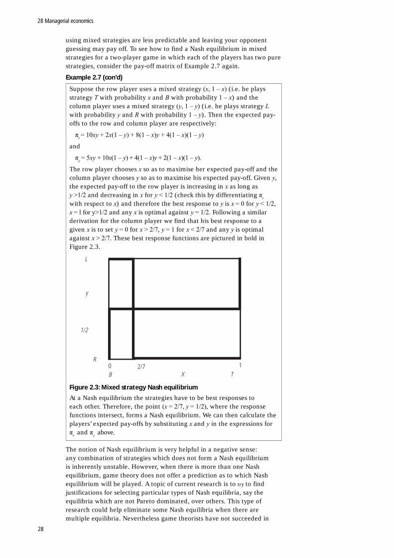
28 Managerial economics
28
using mixed strategies are less predictable and leaving your opponent guessing may pay off. To see how to find a Nash equilibrium in mixed strategies for a two-player game in which each of the players has two pure strategies, consider the pay-off matrix of Example 2.7 again.
Example 2.7 (con’d)
Suppose the row player uses a mixed strategy (x, 1 – x) (i.e. he plays strategy T with probability x and B with probability 1 – x) and the column player uses a mixed strategy (y, 1 – y) (i.e. he plays strategy L with probability y and R with probability 1 – y). Then the expected pay-offs to the row and column player are respectively:
πr = 10xy + 2x(1 – y) + 8(1 – x)y + 4(1 – x)(1 – y)
and
πc = 5xy + 10x(1 – y) + 4(1 – x)y + 2(1 – x)(1 – y).
The row player chooses x so as to maximise her expected pay-off and the column player chooses y so as to maximise his expected pay-off. Given y, the expected pay-off to the row player is increasing in x as long as y >1/2 and decreasing in x for y < 1/2 (check this by differentiating πr with respect to x) and therefore the best response to y is x = 0 for y < 1/2, x = l for y>1/2 and any x is optimal against y = 1/2. Following a similar derivation for the column player we find that his best response to a given x is to set y = 0 for x > 2/7, y = 1 for x < 2/7 and any y is optimal against x > 2/7. These best response functions are pictured in bold in Figure 2.3.
Figure 2.3: Mixed strategy Nash equilibrium
At a Nash equilibrium the strategies have to be best responses to each other. Therefore, the point (x = 2/7, y = 1/2), where the response functions intersect, forms a Nash equilibrium. We can then calculate the players’ expected pay-offs by substituting x and y in the expressions for πr and πc above.
The notion of Nash equilibrium is very helpful in a negative sense: any combination of strategies which does not form a Nash equilibrium is inherently unstable. However, when there is more than one Nash equilibrium, game theory does not offer a prediction as to which Nash equilibrium will be played. A topic of current research is to try to find justifications for selecting particular types of Nash equilibria, say the equilibria which are not Pareto dominated, over others. This type of research could help eliminate some Nash equilibria when there are multiple equilibria. Nevertheless game theorists have not succeeded in
L
y
1/2
R0 2/7 1B X T
Chapter 2: Game theory
29
agreeing on an algorithm which will select the equilibrium that is or should be played in reality.
Prisoners’ dilemmaA class of two-person noncooperative games which has received much attention not only in economics but in social science in general, is the class of prisoners’ dilemma games. The story the game is meant to model concerns two prisoners who are questioned separately, without the possibility of communicating, about their involvement in a crime. They are offered the following deal. If one prisoner confesses and the other does not, the confessor goes free and the other prisoner serves 10 years; if both confess, they each spend seven years in prison; if neither confesses, they each serve a two-year term. This is summarised in the pay-off matrix below.
Confess Don’t
Confess 7,7 0,10
Don’t 10,0 2,2
This game is very easy to analyse: for both players the strategy ‘confess’ dominates. (Remember that you want to minimise the pay-off here!) There is one Nash equilibrium in which both prisoners serve seven-year sentences. What is interesting about this game is that, if the prisoners could set up a binding agreement, they would agree not to confess and serve two years. (This type of model is used to explain difficulties encountered in arms control for example.)
The typical application of the prisoners’ dilemma to managerial economics translates the prisoners’ plight into the situation of duopolists deciding on their pricing policy. If both set a high price they achieve high profits; if both set a low price they achieve low profits; if one firm sets a low price and its rival sets a high price the discounter captures the whole market and makes very high profits whereas the expensive seller makes a loss. At the Nash equilibrium both firms set low prices.
Of course in reality firms do not interact only once but they interact in the market over many years and the question arises whether collusive behaviour could be rationalised in a repeated prisoners’ dilemma game. When the game is played over several periods rather than as a one-shot game, players might be able to cooperate (set a high price) as long as their rival is willing to cooperate and punish when the rival cheats (deviates from cooperation). This possibility of punishment should give players more of an incentive to cooperate in the ion- term. Axelrod (1984) ran a contest in which he asked game theorists to submit a strategy or the repeated version of the prisoners’ dilemma. He then paired the given strategies (some of which were very complicated and required significant computer programming) and ran a tournament. The ‘tit-for-tat’ strategy, which consistently outperformed most of the others, is very simple. This strategy prescribes cooperation as long as the other player cooperates but deviation as soon as and as long as the other player deviates from cooperation. It never initiates cheating and it is forgiving in that it only punishes for one period. If two players use the tit-for-tat strategy they will always cooperate.
Let’s think about what game theory can contribute to understanding players’ behaviour in the repeated prisoners’ dilemma. If the game is repeated a finite number of times then collusive behaviour cannot be rationalised. To see this, remember that the only reason to cooperate is to
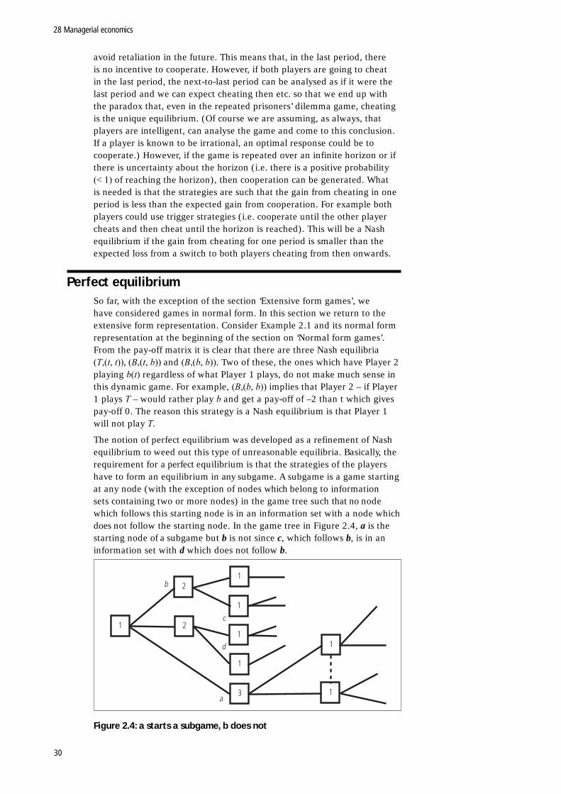
28 Managerial economics
30
avoid retaliation in the future. This means that, in the last period, there is no incentive to cooperate. However, if both players are going to cheat in the last period, the next-to-last period can be analysed as if it were the last period and we can expect cheating then etc. so that we end up with the paradox that, even in the repeated prisoners’ dilemma game, cheating is the unique equilibrium. (Of course we are assuming, as always, that players are intelligent, can analyse the game and come to this conclusion. If a player is known to be irrational, an optimal response could be to cooperate.) However, if the game is repeated over an infinite horizon or if there is uncertainty about the horizon (i.e. there is a positive probability (< 1) of reaching the horizon), then cooperation can be generated. What is needed is that the strategies are such that the gain from cheating in one period is less than the expected gain from cooperation. For example both players could use trigger strategies (i.e. cooperate until the other player cheats and then cheat until the horizon is reached). This will be a Nash equilibrium if the gain from cheating for one period is smaller than the expected loss from a switch to both players cheating from then onwards.
Perfect equilibriumSo far, with the exception of the section ‘Extensive form games’, we have considered games in normal form. In this section we return to the extensive form representation. Consider Example 2.1 and its normal form representation at the beginning of the section on ‘Normal form games’. From the pay-off matrix it is clear that there are three Nash equilibria (T,(t, t)), (B,(t, b)) and (B,(b, b)). Two of these, the ones which have Player 2 playing b(t) regardless of what Player 1 plays, do not make much sense in this dynamic game. For example, (B,(b, b)) implies that Player 2 – if Player 1 plays T – would rather play b and get a pay-off of –2 than t which gives pay-off 0. The reason this strategy is a Nash equilibrium is that Player 1 will not play T.
The notion of perfect equilibrium was developed as a refinement of Nash equilibrium to weed out this type of unreasonable equilibria. Basically, the requirement for a perfect equilibrium is that the strategies of the players have to form an equilibrium in any subgame. A subgame is a game starting at any node (with the exception of nodes which belong to information sets containing two or more nodes) in the game tree such that no node which follows this starting node is in an information set with a node which does not follow the starting node. In the game tree in Figure 2.4, a is the starting node of a subgame but b is not since c, which follows b, is in an information set with d which does not follow b.
Figure 2.4: a starts a subgame, b does not
1
2
2
1
1
1
1
3
1
1
b
c
d
a
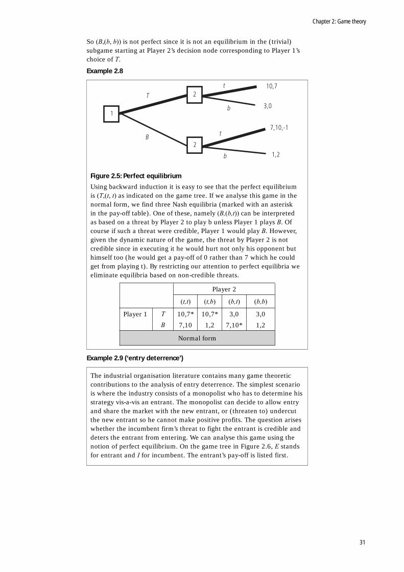
Chapter 2: Game theory
31
So (B,(b, b)) is not perfect since it is not an equilibrium in the (trivial) subgame starting at Player 2’s decision node corresponding to Player 1’s choice of T.
Example 2.8
Figure 2.5: Perfect equilibrium
Using backward induction it is easy to see that the perfect equilibrium is (T,(t, t) as indicated on the game tree. If we analyse this game in the normal form, we find three Nash equilibria (marked with an asterisk in the pay-off table). One of these, namely (B,(b,t)) can be interpreted as based on a threat by Player 2 to play b unless Player 1 plays B. Of course if such a threat were credible, Player 1 would play B. However, given the dynamic nature of the game, the threat by Player 2 is not credible since in executing it he would hurt not only his opponent but himself too (he would get a pay-off of 0 rather than 7 which he could get from playing t). By restricting our attention to perfect equilibria we eliminate equilibria based on non-credible threats.
Player 2
(t,t) (t,b) (b,t) (b,b)
Player 1 T 10,7* 10,7* 3,0 3,0
B 7,10 1,2 7,10* 1,2
Normal form
Example 2.9 (‘entry deterrence’)
The industrial organisation literature contains many game theoretic contributions to the analysis of entry deterrence. The simplest scenario is where the industry consists of a monopolist who has to determine his strategy vis-a-vis an entrant. The monopolist can decide to allow entry and share the market with the new entrant, or (threaten to) undercut the new entrant so he cannot make positive profits. The question arises whether the incumbent firm’s threat to fight the entrant is credible and deters the entrant from entering. We can analyse this game using the notion of perfect equilibrium. On the game tree in Figure 2.6, E stands for entrant and I for incumbent. The entrant’s pay-off is listed first.
1
2
2
10,7
3,0
7,10,-1
1,2
T
B
t
b
t
b
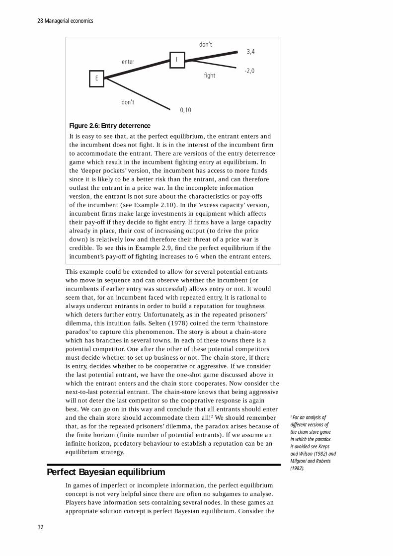
28 Managerial economics
32
Figure 2.6: Entry deterrence
It is easy to see that, at the perfect equilibrium, the entrant enters and the incumbent does not fight. It is in the interest of the incumbent firm to accommodate the entrant. There are versions of the entry deterrence game which result in the incumbent fighting entry at equilibrium. In the ‘deeper pockets’ version, the incumbent has access to more funds since it is likely to be a better risk than the entrant, and can therefore outlast the entrant in a price war. In the incomplete information version, the entrant is not sure about the characteristics or pay-offs of the incumbent (see Example 2.10). In the ‘excess capacity’ version, incumbent firms make large investments in equipment which affects their pay-off if they decide to fight entry. If firms have a large capacity already in place, their cost of increasing output (to drive the price down) is relatively low and therefore their threat of a price war is credible. To see this in Example 2.9, find the perfect equilibrium if the incumbent’s pay-off of fighting increases to 6 when the entrant enters.
This example could be extended to allow for several potential entrants who move in sequence and can observe whether the incumbent (or incumbents if earlier entry was successful) allows entry or not. It would seem that, for an incumbent faced with repeated entry, it is rational to always undercut entrants in order to build a reputation for toughness which deters further entry. Unfortunately, as in the repeated prisoners’ dilemma, this intuition fails. Selten (1978) coined the term ‘chainstore paradox’ to capture this phenomenon. The story is about a chain-store which has branches in several towns. In each of these towns there is a potential competitor. One after the other of these potential competitors must decide whether to set up business or not. The chain-store, if there is entry, decides whether to be cooperative or aggressive. If we consider the last potential entrant, we have the one-shot game discussed above in which the entrant enters and the chain store cooperates. Now consider the next-to-last potential entrant. The chain-store knows that being aggressive will not deter the last competitor so the cooperative response is again best. We can go on in this way and conclude that all entrants should enter and the chain store should accommodate them all!2 We should remember that, as for the repeated prisoners’ dilemma, the paradox arises because of the finite horizon (finite number of potential entrants). If we assume an infinite horizon, predatory behaviour to establish a reputation can be an equilibrium strategy.
Perfect Bayesian equilibriumIn games of imperfect or incomplete information, the perfect equilibrium concept is not very helpful since there are often no subgames to analyse. Players have information sets containing several nodes. In these games an appropriate solution concept is perfect Bayesian equilibrium. Consider the
E
I3,4
-2,0enter
don’t
don’t
fight
0,10
2 For an analysis of different versions of the chain store game in which the paradox is avoided see Kreps and Wilson (1982) and Milgroni and Roberts (1982).
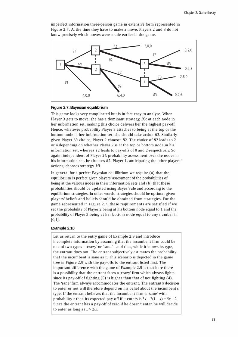
Chapter 2: Game theory
33
imperfect information three-person game in extensive form represented in Figure 2.7. At the time they have to make a move, Players 2 and 3 do not know precisely which moves were made earlier in the game.
Figure 2.7: Bayesian equilibrium
This game looks very complicated but is in fact easy to analyse. When Player 3 gets to move, she has a dominant strategy, B3: at each node in her information set, making this choice delivers her the highest pay-off. Hence, whatever probability Player 3 attaches to being at the top or the bottom node in her information set, she should take action B3. Similarly, given Player 3’s choice, Player 2 chooses B2. The choice of B2 leads to 2 or 4 depending on whether Player 2 is at the top or bottom node in his information set, whereas T2 leads to pay-offs of 0 and 2 respectively. So again, independent of Player 2’s probability assessment over the nodes in his information set, he chooses B2. Player 1, anticipating the other players’ actions, chooses strategy M1.
In general for a perfect Bayesian equilibrium we require (a) that the equilibrium is perfect given players’ assessment of the probabilities of being at the various nodes in their information sets and (b) that these probabilities should be updated using Bayes’ rule and according to the equilibrium strategies. In other words, strategies should be optimal given players’ beliefs and beliefs should be obtained from strategies. For the game represented in Figure 2.7, these requirements are satisfied if we set the probability of Player 2 being at his bottom node equal to 1 and the probability of Player 3 being at her bottom node equal to any number in [0,1].
Example 2.10
Let us return to the entry game of Example 2.9 and introduce incomplete information by assuming that the incumbent firm could be one of two types – ‘crazy’ or ‘sane’ – and that, while it knows its type, the entrant does not. The entrant subjectively estimates the probability that the incumbent is sane as x. This scenario is depicted in the game tree in Figure 2.8 with the pay-offs to the entrant listed first. The important difference with the game of Example 2.9 is that here there is a possibility that the entrant faces a ‘crazy’ firm which always fights since its pay-off of fighting (5) is higher than that of not fighting (4). The ‘sane’ firm always accommodates the entrant. The entrant’s decision to enter or not will therefore depend on his belief about the incumbent’s type. If the entrant believes that the incumbent firm is ‘sane’ with probability x then its expected pay-off if it enters is 3x – 2(1 – x) = 5x – 2. Since the entrant has a pay-off of zero if he doesn’t enter, he will decide to enter as long as x > 2/5.
1
2
2
4,0,0 6,4,0
2,0,00,2,0
0,2,2
2,8,0
0,2,6
3
3
T1
B1
M1
T2
B2
T2
B2
T3
T3
B3
B3
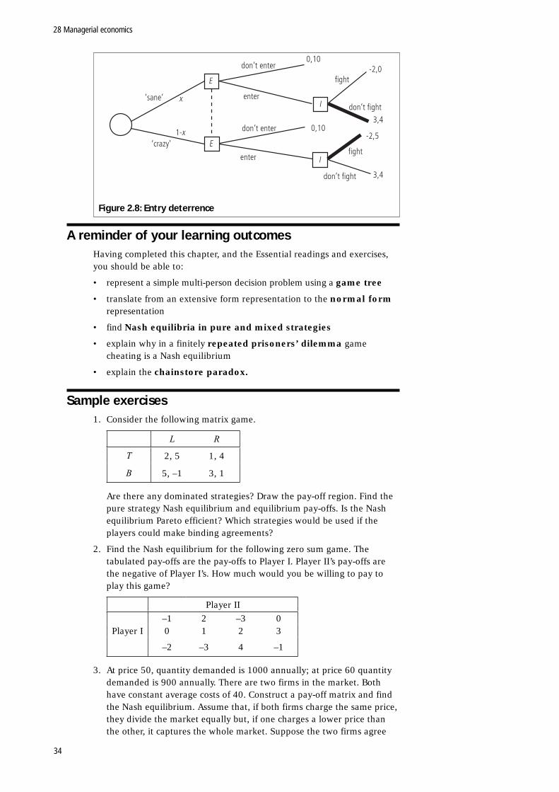
28 Managerial economics
34
Figure 2.8: Entry deterrence
A reminder of your learning outcomesHaving completed this chapter, and the Essential readings and exercises, you should be able to:
• represent a simple multi-person decision problem using a game tree
• translate from an extensive form representation to the normal form representation
• find Nash equilibria in pure and mixed strategies
• explain why in a finitely repeated prisoners’ dilemma game cheating is a Nash equilibrium
• explain the chainstore paradox.
Sample exercises1. Consider the following matrix game.
L R
T 2, 5 1, 4
B 5, –1 3, 1
Are there any dominated strategies? Draw the pay-off region. Find the pure strategy Nash equilibrium and equilibrium pay-offs. Is the Nash equilibrium Pareto efficient? Which strategies would be used if the players could make binding agreements?
2. Find the Nash equilibrium for the following zero sum game. The tabulated pay-offs are the pay-offs to Player I. Player II’s pay-offs are the negative of Player I’s. How much would you be willing to pay to play this game?
Player II–1 2 –3 0
Player I 0 1 2 3
–2 –3 4 –1
3. At price 50, quantity demanded is 1000 annually; at price 60 quantity demanded is 900 annually. There are two firms in the market. Both have constant average costs of 40. Construct a pay-off matrix and find the Nash equilibrium. Assume that, if both firms charge the same price, they divide the market equally but, if one charges a lower price than the other, it captures the whole market. Suppose the two firms agree
E
E
I
I
‘sane’
‘crazy’
don’t enter
don’t enter
enter
enter
fight
fight
don’t fight
don’t fightx
x1-
0,10-2,0
-2,50,10
3,4
3,4
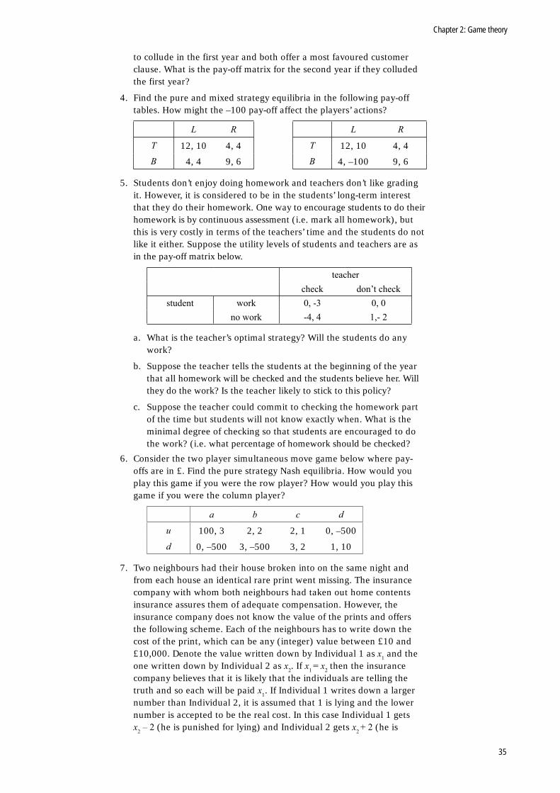
Chapter 2: Game theory
35
to collude in the first year and both offer a most favoured customer clause. What is the pay-off matrix for the second year if they colluded the first year?
4. Find the pure and mixed strategy equilibria in the following pay-off tables. How might the –100 pay-off affect the players’ actions?
L R L R
T 12, 10 4, 4 T 12, 10 4, 4
B 4, 4 9, 6 B 4, –100 9, 6
5. Students don’t enjoy doing homework and teachers don’t like grading it. However, it is considered to be in the students’ long-term interest that they do their homework. One way to encourage students to do their homework is by continuous assessment (i.e. mark all homework), but this is very costly in terms of the teachers’ time and the students do not like it either. Suppose the utility levels of students and teachers are as in the pay-off matrix below.
teachercheck don’t check
student work 0, -3 0, 0no work -4, 4 1,- 2
a. What is the teacher’s optimal strategy? Will the students do any work?
b. Suppose the teacher tells the students at the beginning of the year that all homework will be checked and the students believe her. Will they do the work? Is the teacher likely to stick to this policy?
c. Suppose the teacher could commit to checking the homework part of the time but students will not know exactly when. What is the minimal degree of checking so that students are encouraged to do the work? (i.e. what percentage of homework should be checked?
6. Consider the two player simultaneous move game below where pay-offs are in £. Find the pure strategy Nash equilibria. How would you play this game if you were the row player? How would you play this game if you were the column player?
a b c d
u 100, 3 2, 2 2, 1 0, –500
d 0, –500 3, –500 3, 2 1, 10
7. Two neighbours had their house broken into on the same night and from each house an identical rare print went missing. The insurance company with whom both neighbours had taken out home contents insurance assures them of adequate compensation. However, the insurance company does not know the value of the prints and offers the following scheme. Each of the neighbours has to write down the cost of the print, which can be any (integer) value between £10 and £10,000. Denote the value written down by Individual 1 as x1 and the one written down by Individual 2 as x2. If x1 = x2 then the insurance company believes that it is likely that the individuals are telling the truth and so each will be paid x1. If Individual 1 writes down a larger number than Individual 2, it is assumed that 1 is lying and the lower number is accepted to be the real cost. In this case Individual 1 gets x2 – 2 (he is punished for lying) and Individual 2 gets x2 + 2 (he is
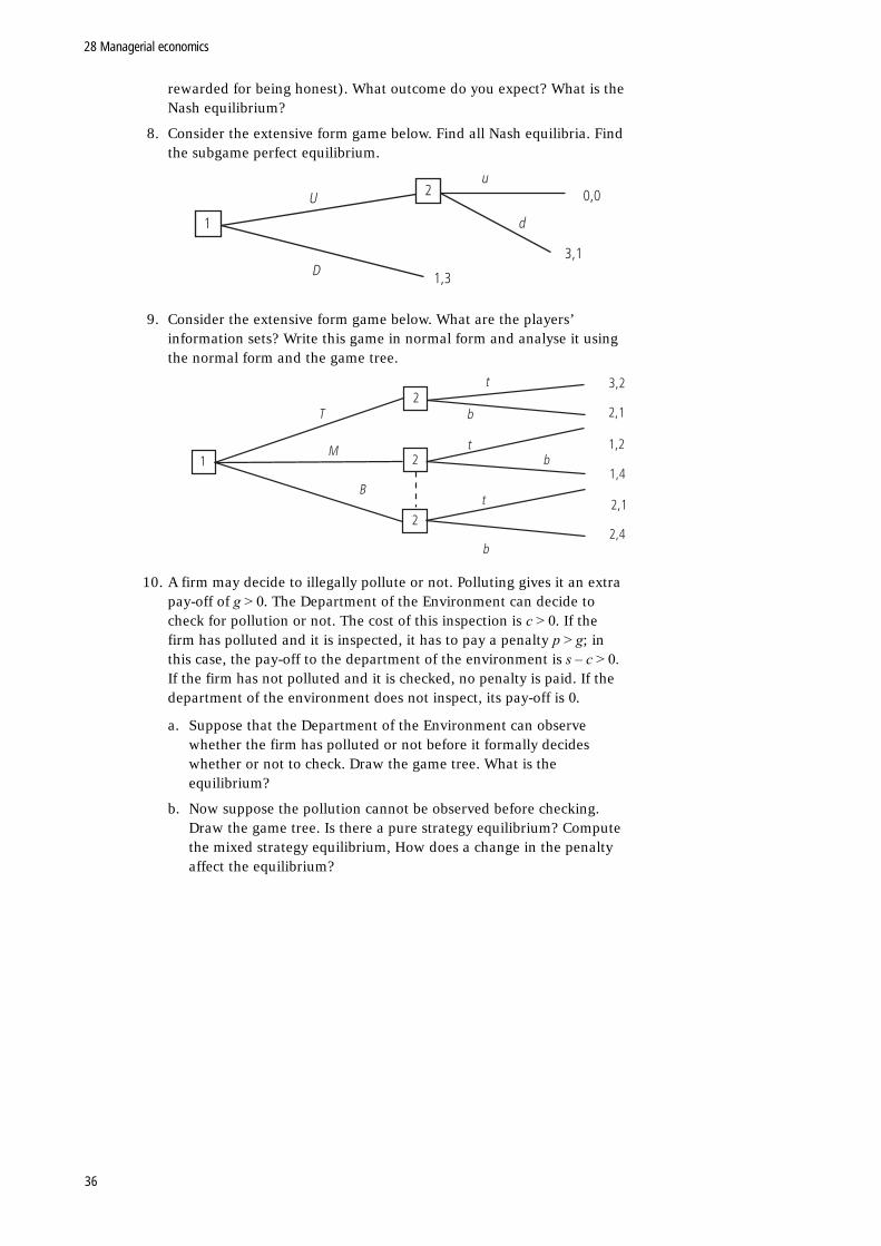
28 Managerial economics
36
rewarded for being honest). What outcome do you expect? What is the Nash equilibrium?
8. Consider the extensive form game below. Find all Nash equilibria. Find the subgame perfect equilibrium.
1
2
3,1
1,3
0,0U
D
d
u
9. Consider the extensive form game below. What are the players’ information sets? Write this game in normal form and analyse it using the normal form and the game tree.
1
2
2
2
T
M
B
t
t
t
b
b
b
3,2
2,1
1,2
1,4
2,1
2,4
10. A firm may decide to illegally pollute or not. Polluting gives it an extra pay-off of g > 0. The Department of the Environment can decide to check for pollution or not. The cost of this inspection is c > 0. If the firm has polluted and it is inspected, it has to pay a penalty p > g; in this case, the pay-off to the department of the environment is s – c > 0. If the firm has not polluted and it is checked, no penalty is paid. If the department of the environment does not inspect, its pay-off is 0.
a. Suppose that the Department of the Environment can observe whether the firm has polluted or not before it formally decides whether or not to check. Draw the game tree. What is the equilibrium?
b. Now suppose the pollution cannot be observed before checking. Draw the game tree. Is there a pure strategy equilibrium? Compute the mixed strategy equilibrium, How does a change in the penalty affect the equilibrium?
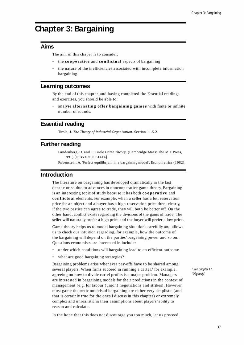
Chapter 3: Bargaining
37
Chapter 3: Bargaining
AimsThe aim of this chaper is to consider:
• the cooperative and conflictual aspects of bargaining
• the nature of the inefficiencies associated with incomplete information bargaining.
Learning outcomesBy the end of this chapter, and having completed the Essential readings and exercises, you should be able to:
• analyse alternating offer bargaining games with finite or infinite number of rounds.
Essential readingTirole, J. The Theory of Industrial Organisation. Section 11.5.2.
Further readingFundenberg, D. and J. Tirole Game Theory. (Cambridge Mass: The MIT Press,
1991) [ISBN 0262061414].Rubenstein, A. ‘Perfect equilibrium in a bargaining model’, Econometrica (1982).
IntroductionThe literature on bargaining has developed dramatically in the last decade or so due to advances in noncooperative game theory. Bargaining is an interesting topic of study because it has both cooperative and conflictual elements. For example, when a seller has a lot, reservation price for an object and a buyer has a high reservation price then, clearly, if the two parties can agree to trade, they will both be better off. On the other hand, conflict exists regarding the divisions of the gains of trade. The seller will naturally prefer a high price and the buyer will prefer a low price.
Game theory helps us to model bargaining situations carefully and allows us to check our intuition regarding, for example, how the outcome of the bargaining will depend on the parties’ bargaining power and so on. Questions economists are interested in include:
• under which conditions will bargaining lead to an efficient outcome
• what are good bargaining strategies?
Bargaining problems arise whenever pay-offs have to be shared among several players. When firms succeed in running a cartel,1 for example, agreeing on how to divide cartel profits is a major problem. Managers are interested in bargaining models for their predictions in the context of management (e.g. for labour (union) negotiations and strikes). However, most game theoretic models of bargaining are either very simplistic (and that is certainly true for the ones I discuss in this chapter) or extremely complex and unrealistic in their assumptions about players’ ability to reason and calculate.
In the hope that this does not discourage you too much, let us proceed.
1 See Chapter 11, ‘Oligopoly’
28 Managerial economincs
38
The alternating offers bargaining gameThe alternating offers bargaining model was formulated and solved fairly recently by Rubinstein (1982). In this model two players have to decide on how to divide an amount of money between them. They alternate in making suggestions about this division. However, as time goes by, the amount of money available shrinks. It turns out that, at the perfect equilibrium of this game, the players agree immediately. To see how this conclusion is arrived at, suppose two players, Bert and Ernie, have a total of £100 to divide between them. Say Bert makes an offer first. He might decide, for example, to keep £70 to himself and offer £30 to Ernie. Ernie will then agree or make a counteroffer. If he agrees, he will get the £30; if he refuses the offer and makes a counteroffer, the £100 ‘cake’ will shrink to £100δ. The discount factor δ (0 < δ < 1) represents the cost of a delay in reaching an agreement (it represents the cost of a strike, for example, where potential output and profit is lost while parties disagree). If the game ends here (i.e. by Bert accepting or rejecting Ernie’s counteroffer) and we assume that if no agreement has been reached both players get zero, it is not hard to see what will happen. (You may want to draw a game tree at this point.) Assuming Bert and Ernie are like the usual self-interested non-altruistic players then, if Ernie decides to make a counteroffer, he will offer Bert one penny which Bert will accept. Ernie in this case ends up with about £100δ. If Bert wants to avoid this predicament he will have to offer Ernie this pay-off from the start so that he keeps £100 (1 – δ) for himself. So if there is only one round of offers, at the perfect equilibrium, Bert will offer £100δ to Ernie and Ernie will accept.
Now consider the same game but Bert will get to make a second offer (i.e. the sequence of moves is Bert, Ernie, Bert). By the time Bert makes his second move, the cake will have shrunk to £100δ2. Now Bert will have the ‘last mover advantage’ and will offer a penny to Ernie. Ernie will anticipate this and offer Bert £100δ2 when he has the opportunity so that he keeps £100δ – £100δ2 = £100δ (1 – δ) for himself. However, Bert can improve on this by offering Ernie £100δ (1 – δ) in the first move and by keeping £100 (1 – δ + δ2) for himself. You should be convinced by now that the subgame perfect equilibrium strategy for each player tells him to make an offer which leaves his opponent very close to indifferent between accepting the offer and continuing the game. As a consequence, the first offer is always accepted.
What happens if we don’t give the players a deadline? Suppose they can keep making offers and counteroffers for an infinite number of periods but, as before, the cake shrinks in each period. Of course this eliminates the ‘last mover advantage’ and we can look for a symmetric equilibrium (players using the same strategy). Also, the equilibrium strategy must be stationary (i.e. it should give the same prescription in each period because, in the infinite version, when an offer has been rejected, the game is exactly as it was before the offer was made except for the shrinking). So, let us assume that Bert offers Ernie £100x and thus keeps £100(1 – x) to himself. Ernie will consider accepting £100x or making an offer of £100x to Bert and keeping £100 (1 – x). Since he should be indifferent between these two options we find δ(1 – x) = x or x = δ/(l + δ). At the equilibrium Bert gets £100/(1 + δ) and Ernie gets £100δ/(1 + δ). In the infinite version of this game it is an advantage to be able to make the first move. Again, as in the finite version, the first offer is always accepted.
Chapter 3: Bargaining
39
As the time between offers and counteroffers shrinks, the discount factor approaches 1 and the asymmetry, caused by who moves first, disappears. It is not very difficult to extend this analysis to allow for different discount factors of the two bargaining parties. The conclusion of this modified bargaining game is that the more patient bargaining partner will get a larger slice of the cake.
Experimental workAlthough the alternating offers bargaining game has a simple ‘solution’ and a stark prediction about the duration of the bargaining (one offer only), the game theoretic findings are not always replicated in experiments. About 10 years ago, when I was a student at LSE, I (and many others) participated in a series of bargaining experiments. Subjects were paired to an unknown bargaining partner and could only communicate via a formal computer program with their partner who was sitting in a different room. Experiments of this type generally show that ‘real’ players have a tendency to propose and accept what they consider a fair offer while rejecting what they consider a mean offer even if this rejection means they will be in a worse position. If you were offered one penny in the last round of the game in this section, would you accept?
Incomplete information bargainingThe alternating offers bargaining game does not look very appealing as a paradigm for real life bargaining situations in which disagreement is common and costly negotiations take place for several weeks or months. It turns out that to generate delayed agreement you have to assume that the players do not know all the information there is to know about their opponent (i.e. players have private information). In particular, players may have private information about their reservation price when bargaining over the sale of an item. Models of incomplete information bargaining can be extremely complex and I will not discuss them in general or even give an overview.2 Instead, I will show you in a simple example that inefficiencies can occur. This means that, if it were possible to get both players to reveal their valuations truthfully, they could both be made better off. It is precisely because players are hiding their valuations that there are costly delays before an agreement is reached.
Two players, a seller and a buyer, are trying to come to an agreement about the price at which a good will be sold. The seller has a valuation (or reservation price) of 1 or 3, equally likely. The buyer has valuation 2 or 4, equally likely. I will refer to a player as being of type i if he has valuation i. The seller moves first and offers to sell for a price of 2 or 4. The buyer always accepts an offer of 2 but may reject a price of 4. If the buyer rejects, the seller can offer a price of 2 or 4 and the buyer has another chance to accept or reject. If there is delay any pay-offs in the second period are discounted using a discount factor ds for the seller and db for the buyer. Table 1 contains the possible strategies for each type of player and the pay-offs corresponding to each possible strategy pair. The first pay-off listed is the buyer’s. Note that a seller of type 3 will never set the price equal to 2 and that a buyer of type 2 is never willing to buy at price 4. This restricts the number of strategies we have to consider.
2 For an advanced treatment of this material see, for example, Fudenbergand Tirole (1991) Chapter 10

28 Managerial economincs
40
Seller type 1 Seller type 3
ask 2 ask 4, then 2 ask 4, then 4 always ask 4buyer type 2always rejects 4
(0, 1) (0, ds) (0, 0) (0, 0)
buyer type 4reject 4 once
(2, 1) (2db, ds) (0, 3ds) (0, ds)
do not reject (2, 1) (0, 3) (0, 3) (0, 1)
For a buyer of type 4, rejecting a price of 4 in the first period weakly dominates accepting price 4 immediately. If we eliminate the last row in the table then, for a seller of type 1, asking a price of 2 dominates asking 4 first and then asking 2 so that we can eliminate the second column in the table. Given that the seller of type 1 thinks that the buyer he faces is equally likely to be of type 2 as of type 4, asking 2 gives him an expected pay-off of 1 whereas asking 4 twice gives him an expected pay-off of 0(1/2) + (3ds)(1/2). Thus the seller of type 1 asks 2 if 1 > (3ds/2) or ds < 2/3. It follows that, if ds > 2/3, there is no trade, at the equilibrium, between a seller of type 1 and a buyer of type 2 which is clearly inefficient. If ds < 2/3 there is an inefficient delay in the agreement between a seller of type 1 and a buyer of type 4 at the equilibrium. There is also an inefficient delay of the agreement between a seller of type 3 and a buyer of type 4.
A reminder of your learning outcomesBy the end of this chapter, and having completed the Essential reading and activities, you should be able to:
• analyse alternating offer bargaining games with finite or infinite number of rounds.
Sample exerciseConsider the alternating offers bargaining game over £100, with Bert making the first offer and Ernie making a counter offer if he wants to. Suppose Bert has an outside option of £50, that is, at any point during the game, Bert can stop bargaining and get £50 (discounted if he gets it after the first period). If Bert takes his outside option, Ernie gets zero. How does this effect the equilibrium strategies and pay-offs?