management of produced water in oil and gas …

MANAGEMENT OF PRODUCED WATER IN OIL AND GAS OPERATIONS

A Thesis

by

CHIRAG PATEL

Submitted to the Office of Graduate Studies of Texas A&M University

in partial fulfillment of the requirements for the degree of

MASTER OF SCIENCE

December 2004

Major Subject: Petroleum Engineering

CORE Metadata, citation and similar papers at core.ac.uk

Provided by Texas A&M University

https://core.ac.uk/display/147123617?utm_source=pdf&utm_medium=banner&utm_campaign=pdf-decoration-v1

MANAGEMENT OF PRODUCED WATER IN OIL AND GAS OPERATIONS

A Thesis

by

CHIRAG PATEL

Submitted to Texas A&M University

in partial fulfillment of the requirements for the degree of

MASTER OF SCIENCE

Approved as to style and content by:

_______________________________ Maria A. Barrufet

(Chair of Committee)

_______________________________ Peter P. Valko

(Member)

_______________________________ Dragomir B. Bukur

(Member)

_______________________________ Stephen A. Holditch

(Head of Department)

December 2004

Major Subject: Petroleum Engineering

iii

ABSTRACT

Management of Produced Water in Oil and Gas Operations. (December 2004)

Chirag Patel, B.E., Nirma Institute of Technology, India

Chair of Advisory Committee: Dr. Maria A. Barrufet

Produced water handling has been an issue of concern for oil and gas

producers as it is one of the major factors that cause abandonment of the producing well.

The development of effective produced water management strategies poses a big

challenge to the oil and gas industry today. The conversion of produced water into

irrigation or fresh water provides a cost effective tool to handle excessive amounts of the

produced water. In this research we proposed on-site produced water treatment units

configured to achieve maximum processing throughput. We studied various advanced

separation techniques to remove oil and dissolved solids from the produced water. We

selected adsorption as the oil removing technique and Reverse Osmosis (RO) as the

dissolved solids removing technique as being the best for our purpose. We performed

experiments to evaluate operating parameters for both adsorption and RO units to

accomplish maximum removal of oil and dissolved solids from the produced water. We

compared the best models fitting the experimental data for both the processes, then

analyzed and simulated the performance of integrated produced water treatment which

involves adsorption columns and RO units.

The experimental results show that the adsorption columns remove more than

90% of the oil and RO units remove more than 95% of total dissolved solids from the

produced water. The simulation results show that the proper integration and configuration

of adsorption and RO units can provide up to 80% efficiency for a processing throughput

of 6-8 gallons per minute of produced water. From an oil and gas producer’s viewpoint

output from the produced water treatment system is a revenue generating source. The

system is flexible and can be modified for the applications such as rangeland restoration,

reservoir recharge and agricultural use.

iv

ACKNOWLEDGEMENTS

I would like to take this opportunity to thank all those who helped and assisted me

in completing this thesis. I extend my deepest gratitude to Dr. Maria A. Barrufet, advisor

and chair of my committee, and to Dr. Peter P. Valko, committee member, for guiding

and encouraging me towards accomplishment of my graduate studies.

I would like to thank Dr. Dragomir B. Bukur for serving on my committee and for

providing his valuable suggestions.

I also thank Adrian for his guidance, suggestions and help in performing

experiments. I also thank Mr. David Burnett for his valuable contribution to this project.

I would like to thank Dr. Robert P. Mahoney and Mr. Jonathan Fabri from

Polymer Ventures Inc., for providing technical support.

v

TABLE OF CONTENTS

Page

ABSTRACT……………………………………………………………………………..iii

ACKNOWLEDGEMENTS……………………………………………………...…….....iv

TABLE OF CONTENTS.…………………………………………………………….......v

LIST OF FIGURES.....................................................................................................…..vii

LIST OF TABLES…………………………………………………………………….......x

CHAPTER

I INTRODUCTION– EFFECTIVE MANAGEMENT OF PRODUCED

WATER ............................................................................................................... 1

1.1 Introduction.............................................................................................. 1 1.2 Conversion of produced water-A new approach ..................................... 2

1.2.1 A background of produced water treatment.................................... 2 1.2.2 Distributed water processing and recycling.................................... 2

II OIL REMOVAL FROM THE PRODUCED WATER ....................................... 5

2.1 Measurement of total oil content (TOC) in water.................................... 5 2.1.1 Oil in water analysis by TOC-700 analyzer.................................... 6 2.1.2 Oil in water analysis by TD-500 analyzer .................................... 11

2.2 Selection of adsorption for oil removal from produced water............... 13 2.3 Adsorption terminologies ...................................................................... 17 2.4 Evaluation of new organoclay adsorbent for oil removal...................... 19

2.4.1 Packed bed adsorption experiments.............................................. 20 2.5 Data acquisition and presentaion ........................................................... 25

III DISSOLVED SOLID REMOVAL FROM THE PRODUCED WATER......... 27

3.1 Selection of reverse osmosis (RO)......................................................... 28 3.2 RO terminologies................................................................................... 27 3.3 Experimental setup ................................................................................ 29 3.4 Data acquisition and presentaion ........................................................... 31

vi

CHAPTER Page

IV RESULTS AND DISCUSSION........................................................................ 32

4.1 Packed bed adsorption ........................................................................... 32 4.1.1 Effect of contact time.................................................................... 32 4.1.2 Effect of size of organoclay particle ............................................. 34 4.1.3 Effect of feed concentrations ........................................................ 37 4.1.4 Effect of type of oils ..................................................................... 40 4.1.5 Change in organoclay structure .................................................... 42

4.2 RO results and discussion...................................................................... 42 4.2.1 Effects of various parameters on permeate recovery fraction ...... 42 4.2.2 Effects of various parameters on salt removal.............................. 44

V MODELING AND SIMULATION................................................................... 47

5.1 Literature review.................................................................................... 47 5.2 A new approach for modeling of adsorption ......................................... 52 5.3 Modeling of RO..................................................................................... 57 5.4 Case studies - Treatment of produced water......................................... 59

5.4.1 Case study 1-CBM produced water treatment .............................. 62 5.4.2 Case study 2-West Texas produced water treatment .................... 64

VI CONCLUSIONS AND RECOMMENDATIONS ............................................ 67

6.1 Conclusions............................................................................................ 67 6.2 Recommendations.................................................................................. 67

NOMENCLATURE……………………………………………………………………..69

REFERENCES........……………………………………………………………………..71

VITA……………………………………………………………………………………..75

vii

LIST OF FIGURES

FIGURE Page

1.1 A schematic of produced water treatment cycle, a possible DWPR

configuration ............................................................................................................3

2.1 Calibration curve for TOC-700 analyzer that analyzes oil present in water..........10

2.2 Calibration curve for TD-500 analyzer that analyzes oil present in water ............12

2.3 A schematic of FTS PHASE3 coalescer.................................................................13

2.4 Effects of feed concentration and residence time on oil content of outlet

from coalescer........................................................................................................15

2.5 Effects of feed concentrations and residence time on oil removal efficiency

of coalescer ............................................................................................................16

2.6 A schematic of experimental setup for adsorption operation ................................21

2.7 SEM image of un-crushed organoclay particle......................................................22

2.8 Diatoms provide porous structure to organoclay ...................................................22

2.9 Reduction of size of organoclay particle in laboratory..........................................23

2.10 A conceptual diagram showing effect of particle size reduction

on MTZ ..................................................................................................................24

3.1 Schematic of spiral wound RO membrane in operations.......................................28

3.2 Laboratory unit to perform pilot scale RO operations ...........................................30

4.1 Comparison of breakthrough curve for experiments with different EBCT ...........34

4.2 Concentration front is sharper with reduced particle size......................................36

4.3 Comparison of breakthrough behavior for experiments with different size

of organoclay particles...........................................................................................36

viii

FIGURE Page

4.4 Comparison of breakthrough behavior for experiments with different feed

concentrations .........................................................................................................38

4.5 Results for an experiment with produced water as feed ........................................39

4.6 Breakthrough behavior for experiments with different types of oil in feed ..........41

4.7 1000X magnification of organoclay particle after adsorption

(left hand side) and before adsorption (right hand side) .......................................42

4.8 Effects of TDS content and flow rate of feed on permeate flux at various

transmembrane pressure.........................................................................................43

4.9 Effects of TDS content and flow rate of feed on permeate recovery

fraction at various transmembrane pressure ..........................................................44

4.10 Effects of TDS content and flow rate of feed on salt rejection at

various transmembrane pressure............................................................................45

4.11 Effects of TDS content and flow rate of feed on permeate

concentration at various transmembrane pressures................................................46

5.1 A schematic diagram of packed bed adsorption column .......................................47

5.2 Fitting an empirical model to the breakthrough data for experiment G ................52

5.3 Fitting hyperbolic function to the experimental data of percentage of oil

adsorbed with time.................................................................................................53

5.4 A straight line fit to the experimental data of oil adsorption

vs. oil inflow ..........................................................................................................54

5.5 Linear fitting of an empirical model to estimate adsorption coefficient................55

ix

FIGURE Page

5.6 New empirical model fits the data for experiment G.............................................56

5.7 Model accurately fits the experimental permeate recovery data ...........................58

5.8 Model accurately predicts experimental salt rejection data...................................59

5.9 A schematic of sequence of operations for conversion of produced water

into a fresh water source ........................................................................................60

5.10 Adsorption canister and RO unit specifications for CBM produced water

treatment case.........................................................................................................62

5.11 Simulation run showing TDS and TOC content in permeate stream or

final outlet of produced water treatment system for CBM produced

water treatment.......................................................................................................63

5.12 Adsorption canister and RO unit specifications for West Texas

produced water treatment case...............................................................................65

5.13 Simulation run showing TDS and TOC content in permeate stream

or final outlet of produced water treatment system for West Texas

produced water treatment......................................................................................66

x

LIST OF TABLES

TABLE Page

2.1 Properties of proposed new adsorbent organoclay PS18385 for oil removal

from produced water ..............................................................................................20

2.2 A list of parameters to be acquired in each adsorption experiment .......................26

4.1 Experiments with same feed concentration, particle size but different

EBCT .....................................................................................................................33

4.2 Experiments with different feed concentration and particle sizes .........................35

4.3 Experiments with different feed concentrations and approximately same

EBCT ...................................................................................................................37

4.4 Experimental results with produced water as feed. The column had not

received the breakthrough (sharp increase in concentration is not

observed)...............................................................................................................39

4.5 Experimental parameters for experiments with different types of

oil present in feed...................................................................................................40

5.1 List of dynamic parameters in produced water treatment simulator......................61

1

CHAPTER I

INTRODUCTION – EFFECTIVE MANAGEMENT OF PRODUCED WATER

1.1 Introduction

The composition of produced water is strongly field-dependent and includes a

variety of inorganic and organic compounds. Produced water contains small amounts of

emulsified oil, organic compounds including dissolved hydrocarbons, organic acids,

phenols and traces of chemicals added during production, inorganic compounds,

suspended solids, dissolved solids and natural low-radioactive elements.

The most popular option to handle produced water is to re-inject it back into the

formation. Produced water re-injection (PWRI) requires minimal or modified treatment

before injection to obtain better results, but the injectivity decreases with time. As the

reservoir matures injected produced water swipes through to the producing zone and

water production increases with time which causes abandonment of the well.

Transportation of produced water from production to injection sites increases re-injection

costs. Furthermore, the produced water rate can be as high as 10 bbl per bbl of

hydrocarbons and it may not always be feasible to re-inject all produced water volumes.

Several options are being employed to handle this remaining excessive amount of

produced water. Disposal of produced water is costly (as high as $4/bbl) depending upon

its makeup and transportation volumes, which must be handled and also have to face

stringent environmental regulations. There is a need for an effective produced water

management strategy that handles large amounts of produced water and meets

environmental regulations1.

Approximately four million barrels of produced water is produced along with oil

and gas per year in the state of Texas. In West Texas Coal Bed Methane (CBM)

producing regions the fresh water is a scarcity and produced water is in excessive

amount. If properly treated, produced water can be a source of fresh water and can prove

beneficial to the society particularly in arid areas. Many efforts are being made to convert

CBM produced water into usable water by EPA, DOE and other institutions.

_____________

This thesis follows the style of SPE Reservoir Evaluation & Engineering.

2

1.2 Conversion of produced water – A new approach

1.2.1 A background of produced water treatment

Evans et al.2 have discussed several produced water handling options and

associated dangers. Disposal, re-injection and treatment of produced water are the

available options. Produced water disposal requires meeting stringent environmental

regulations and requires proper treatment before the disposal. Mackay et al.3 described

risk involved in re-injection. Produced water re-injection requires skillful planning and

treatment to meet the quality of re-injection water to avoid formation damage. Jun Wan et

al.4 showed treatment of produced water before re-injection gives better performance.

Alonzo et al.5 assessed the produced water treatments as well as disposal practice and

addressed the research needs in this area. Hughes et al.6, Tao et al.7 and Tsang et al.8

discussed conversion of produced water into irrigation or drinking quality water. The

review of various produced water treatment technologies and its applications for Coal

Bed Methane (CBM) operators are discussed in literature9.

The general approach for produced water treatment is de-oiling and de-

mineralizing before disposal or utilization. The use of centrifuge10, air-floaters,

emulsifiers, hydroclones11, membrane separators12 and adsorbers13 to remove oil and

grease from the produced water is discussed in literature. Several methods such as micro-

filtration (MF), ultra-filtration (UF), ion exchange, and reverse osmosis (RO) 14, 15 are

available for de-mineralization purpose. Roberts15 showed considerable reduction in de-

mineralization cost with RO operation. Siddiqui16 suggested use of RO units to achieve

maximum salt rejection and efficiency based on experimental results. The literature

discussed above, do not provide sufficient information on modeling of separation

technique for produced water treatment application. In this thesis, we model the best

available technology and provide a static and a dynamic model of this technology. The

static model refers to equipment sizing, while the dynamic model takes into account the

process conditions. Our model can be used for a pilot scale operation and can be scaled

up to a larger throughput.

1.2.2 Distributed water processing and recycling

There is a need to design and develop a general and effective produced water

treatment system. We discussed the issue and approached to initiate development of

3

produced water treatment unit that would be feasible for field application. A Distributed

Water Processing and Recycling (DWPR) system is being developed at Texas A&M

University to treat produced water with a rate of 6 GPM or with a flux of 0.086 GPM/ft2

at a pilot scale. It involves combinations of primary and polishing de-oiling and de-

mineralizing units. Figure 1.1 shows a schematic of a possible DWPR system. Flux is

defined as the ratio of the flow rate to the surface area of RO membrane.

Produced WaterStorage

ROAdsorption / Oil Removal

Organoclay

Hydroclone / RotaryOil-Water Separation

Coalescer / GravityOil-Water-Solid Separation

PW

Oil

Water

Adsorben In

Microfiltration

Fig. 1.1 – A schematic of produced water treatment cycle, a possible DWPR configuration.

The objectives accomplished in this research are;

1. Testing of new adsorbent organoclay-PS12385 for oil removal from produced

water. The organocaly-PS12385 is structurally modified clay that does not swell

upon adsorption of oil.

2. Testing of RO membrane-SWC 1 4040 for dissolved solids removal.

3. Development of models to fit experimental data for oil adsorption column and for

salt removal.

4

4. Estimation of operating parameters for oil adsorption columns and RO units.

5. Simulation of transient performance of integrated adsorption-RO system.

5

CHAPTER II

OIL REMOVAL FROM THE PRODUCED WATER

2.1 Measurement of total oil content (TOC) in water

TOC analysis of oil containing samples and samples processed by oil removal

units determines the performance of the oil removal unit in terms of oil removal capacity

and efficiency. The definition of TOC is field specific. Environmental Protection Agency

(EPA) defines crude oil content in water as the amount of hydrocarbons that can be

extracted by solvents such as n-Hexane, Xylene or Freon in acidic media. Alternately,

TOC can be defined as the amount of hydrocarbons in sample that releases carbon

dioxide upon oxidation in acidic media. The values of the TOC obtained from both

solvent extraction and oxidation may not be the same since the solvent extraction process

only extracts aromatic hydrocarbons while oxidation process converts total organic

carbon (aromatic, aliphatic etc) into carbon dioxide.

Calibration of the TOC analyzer is crucial in any oil analysis technique. A

calibration factor is obtained by calibrating the analyzer response signal for samples with

known oil concentrations. The calibration factors can be different for different types of

oil present in the sample. For example, the calibration factor obtained for samples

containing kerosene is different from the calibration factor obtained for samples

containing diesel. However according to EPA, if the analyzer is calibrated with samples

containing crude oil, it is sufficient for analyzing TOC of the sample.

TOC-700 (manufactured by O.I. Analytical) analyzer works on the principle of

oxidation of total organic carbon. TD-500 (manufactured by Turned Design Inc.) works

on the principle of solvent extraction of hydrocarbons. For non-uniformly mixed or

emulsified samples TOC-700 may not provide accurate results as the amount of the

sample injected into the analyzer may not be representative of the original sample. TD-

500 eliminated this problem by extracting oil phase of the sample and analyzing only

extracted oil phase. The main advantage of TD-500 is that it enables the user to use large

amounts of sample (more than 50 ml compared to 1 µl-2 ml in case of TOC-700) for

analysis which reduces the chances of inaccuracy because the larger the amount of

sample the higher the chances of good representation of the original sample.

6

In this work TOC-700 was used to analyze kerosene-water emulsions. To match

TOC analysis with the EPA standard a TD-500 was used to analyze crude oil-water

emulsion and produced water.

2.1.1 Oil in water analysis by TOC-700 analyzer

The analyzer is capable of measuring Total Inorganic Carbon (TIC), TOC,

Dissolved Organic Carbon (DOC), Suspended Organic Carbon (SOC), Purgeable

Organic Carbon (POC), Purgeable Organic Halide (POX) and Non-Purgeable Organic

Carbon (NPOC). Only TOC analysis will be discussed in detail since the analyzer was

only utilized to measure TOC of the sample.

TOC is determined by the measurement of carbon dioxide released by chemical

oxidation of the organic carbon in the sample. First an appropriate amount of sample is

injected into the reaction chamber by manual injection or auto-sampling loop. The

sample is acidified to purge the TIC. Sodium persulfate, a strong oxidizer is added next.

The oxidant quickly reacts with organic carbon in the sample at 100oC to form carbon

dioxide. When the oxidation reaction is completed, the carbon dioxide is purged form the

solution, concentrated by trapping and then desorbed and detected by a non dispersive

infrared (NDIR) detector. NDIR converts the amount of carbon dioxide into equivalent

mili-volt (mV) signal. The calibration factor converts the mV signal into ppm of oil.

It is essential to calibrate the analyzer before using it. The calibration factor

relates the detected amount of carbon dioxide and hence mV response of the NDIR to the

mass of organic carbon originally present in the sample.

Calibration of TOC-700

The calibration process is described in the following sections,

1. Preparation of reagent blanks.

2. Preparation of samples of various kerosene concentrations.

3. Sample injection into the analyzer.

4. Sample oxidation in reaction chamber.

5. Purging and trapping of released carbon dioxide.

7

6. Detection of carbon dioxide by NDIR and display result in ppm of TOC.

1. Preparation of reagent blanks.

Reagent water: Water used for preparing the reagent blanks should contain less than 200

ppb of TOC. We used distilled or deionized water.

Sodium persulfate (100 g/L): It is prepared by dissolving 100 g sodium persulfate into

reagent water (1 liter total volume). The solution is stirred and then heated in a bottle

with loose lid until the solution just comes to boil. As soon as the solution appears to start

boiling the lid is tighten and the bottle is immersed in cold water. This procedure purifies

the persulfate solution by reducing TOC content of reagent water that was added during

preparation of the solution.

Phosphoric Acid (5% vol/vol): Acid for TIC removal is prepared by dissolving

phosphoric acid (85% purity) into reagent water. A volume of 5 ml phosphoric acid (85%

purity) is mixed with 95% reagent water to make 5% vol/vol solution.

2. Preparation of samples of various kerosene concentrations.

The NDIR linearity range of detection is 0-1000 mili-volt (mV). The

concentration of kerosene in samples should not cause the mV response of NDIR to go

beyond 1000 mV. Different concentrations of kerosene were tried and by observation the

data were selected for the concentrations that provided less than 1000 mV response. The

calibration curve is obtained by plotting these data. We tried samples with kerosene

concentration ranging from 20 – 800 ppm for calibration purpose. For measuring a

sample having concentration more than 800 ppm, we diluted the samples.

3. Sample injection into the analyzer.

One method for charging the sample to the analyzer is via a syringe (sampling

volume of 5 - 100µL). Another is loop sampling, in which the sample loop introduction

system allows repeatable analysis over a wide range of concentrations while avoiding the

inherent dead volumes of syringe-based systems. On-line total organic carbon analyzer

systems have an analyzer that is mounted in a process line and the sample is introduced

via a automatic valve. Via auto samplers are another way to introduce the sample. The

liquid-sample transfer auto-sampler removes specific sample volumes from a standard

8

vial and transfers the sample to the common analysis vessel. A sample carousel is loaded

with up to fifty vials and placed in the auto-sampler for unattended analysis. In addition

to measuring total organic carbon, total organic carbon analyzers may sometimes be used

to detect total carbon, total inorganic carbon, and purgeable and nonpurgeable organic

carbon.

Kerosene-water forms a very unstable emulsion therefore continuous stirring is

necessary to avoid the two components to get separated. Because of stirring air is added

to the sample and that causes the error in estimation of TOC. For smaller sample injection

volume (0.025 ml to 0.5 ml) the air present in it causes error. By using larger sample (1

ml) injection volume the possibility of error due to air is minimized greatly. Auto

sampling loop was used for analysis of each sample that allows injection of 1 ml of

sample automatically.

4. Chemical oxidation of sample in reaction chamber.

The oxidation of the sample by sodium persulfate is carried out in an oxidization

chamber at user defined temperature (we set the reaction temperature at 180 oC to ensure

complete oxidation). The default reaction time is 5 mins. In some cases the default time

was not long enough to oxidize the sample completely and that caused error in TOC

quantification. This caused non-repeatability of the results. The reaction time can be

extended further by user. We tried upto 8 min of reaction time.

The volumes of acid and persulfate solution are also determined by the user. The

determination of volume of acid and oxidizer requires observation and experience with

the equipment. We used excess amount of acid and oxidizer to ensure the completion of

the reaction. The volume of reagents and the time of reaction should be large enough to

oxidize the sample completely. If the chemical formula of the sample is known the

volumes can be determined by stoichiometric calculations. If the chemical formula is

unknown trial and error method is employed. Different volumes of reagents and reaction

times are tried until the complete oxidation of the sample is obtained in quantification.

9

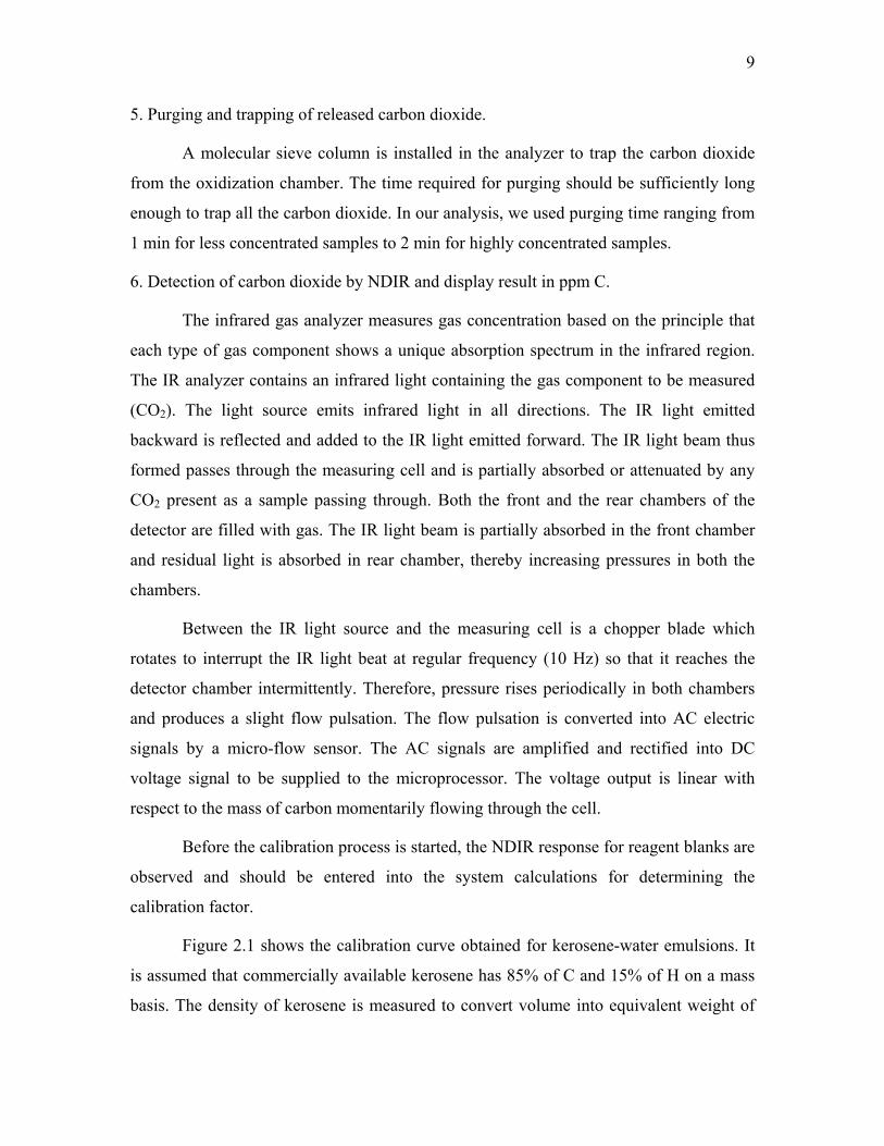
5. Purging and trapping of released carbon dioxide.

A molecular sieve column is installed in the analyzer to trap the carbon dioxide

from the oxidization chamber. The time required for purging should be sufficiently long

enough to trap all the carbon dioxide. In our analysis, we used purging time ranging from

1 min for less concentrated samples to 2 min for highly concentrated samples.

6. Detection of carbon dioxide by NDIR and display result in ppm C.

The infrared gas analyzer measures gas concentration based on the principle that

each type of gas component shows a unique absorption spectrum in the infrared region.

The IR analyzer contains an infrared light containing the gas component to be measured

(CO2). The light source emits infrared light in all directions. The IR light emitted

backward is reflected and added to the IR light emitted forward. The IR light beam thus

formed passes through the measuring cell and is partially absorbed or attenuated by any

CO2 present as a sample passing through. Both the front and the rear chambers of the

detector are filled with gas. The IR light beam is partially absorbed in the front chamber

and residual light is absorbed in rear chamber, thereby increasing pressures in both the

chambers.

Between the IR light source and the measuring cell is a chopper blade which

rotates to interrupt the IR light beat at regular frequency (10 Hz) so that it reaches the

detector chamber intermittently. Therefore, pressure rises periodically in both chambers

and produces a slight flow pulsation. The flow pulsation is converted into AC electric

signals by a micro-flow sensor. The AC signals are amplified and rectified into DC

voltage signal to be supplied to the microprocessor. The voltage output is linear with

respect to the mass of carbon momentarily flowing through the cell.

Before the calibration process is started, the NDIR response for reagent blanks are

observed and should be entered into the system calculations for determining the

calibration factor.

Figure 2.1 shows the calibration curve obtained for kerosene-water emulsions. It

is assumed that commercially available kerosene has 85% of C and 15% of H on a mass

basis. The density of kerosene is measured to convert volume into equivalent weight of

10

kerosene. For example, 1 ml of kerosene is equivalent to 0.81 gm. The C content in the

sample is 0.85 times the 0.81 gm. Finally, C content is calculated as mg of C per liter

volume of sample.

y = 0.80016850xR2 = 0.97989449

0

200

400

600

0 200 400 600 800Analyzer response, mV

Sam

ple

conc

entra

tion,

ppm

Fig. 2.1 – Calibration curve for TOC-700 analyzer that analyzes oil present in water. The ppm concentration is plotted against the net mV response from NDIR. Net

mV response is the value obtained by subtracting mV response of reagent blanks and

distilled water from the mV response of the sample, e.g. kerosene-water emulsions. The

curve is reasonably linear and covers wide range of concentration. Kerosene-water

emulsions having concentration higher than the maximum limit of the calibration curve

should be further diluted as without dilution the mV response would not be linear.

11

2.1.2 Oil in water analysis by TD-500 analyzer

TD-500 oil in water analyzer measures the oil content in the oily water containing

crude oil or gas condensates using UV fluorescence. It works on produced water, de-

salter tail water, and crude storage tank water and in any application where crude oil may

be in contact with the water.

TD-500 oil in water meter uses an easy to use solvent extraction procedure with

high accuracy and repeatability. The standard procedure of solvent extraction is specified

by EPA-1664A method better known as FastHex method of analysis. The analysis

method is compatible with all popular solvents including n-Hexane, Vertrel, AK-225,

Freon, Xylene and others. The sample analysis time is less than 4 minutes.

Calibration and sample analysis

1. Sample Preparation

A 90 ml volume of the sample to be analyzed is collected in a graduated cylinder.

The pH of the sample is adjusted below value of 2 by adding hydrochloric acid or sulfuric

acid. Solvent is added as 1 part in 9 parts of the sample on volume basis. The cylinder is

rigorously shacked for couple of minutes. Solvent extracts soluble oil present in the

sample and the two layers are formed. The extract layer contains solvent and oil extracted

from the sample. The extract is carefully separated and collected into a separate cylinder

or flask. The extract is analyzed by TD-500.

2. Sample Analysis

Before analyzing a sample the TD-500 meter is calibrated using standard samples.

The standard samples of known oil content are prepared. We measured the density of oil

to obtain equivalent weight per unit volume of oil. As a starting point, we prepared a

mixture of 1 ml of oil in 9 ml of n-Hexane. This mother solution is diluted with various

volumes of n-Hexane to create samples with different oil concentrations. TD-500 meter is

set on calibration mode. The TOC value of standard is entered into the analyzer. In this

case we obtained amount of aromatic oil content in sample unlike the case of TOC-700

where we obtained amount of total organic carbon content in sample.

12

The appropriate volume (0.075 ml to 1 ml) of extract is collected in clean minicell

cuvettes or 8 mm round cuvettes. The cuvette filled with the extract is placed in a cuvette

adapter. The adapter fits into the sample compartment of the analyzer. The analyzer

responds within 5 seconds. The value of calibration factor is calculated by the analyzer

according to the TOC content of standard and response of the analyzer.

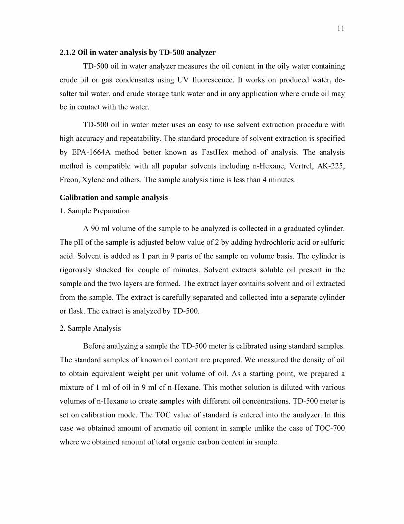
Figure 2.2 shows the calibration curve for TD-500 prepared using crude oil (380

API)-water emulsions.

y = 1.34320045xR2 = 0.98127555

0

200

400

600

800

1000

0 200 400 600 800TD-500 response, mV

Sam

ple

conc

entra

tion,

ppm

Fig. 2.2 – Calibration curve for TD-500 analyzer that analyzes oil present in water.

After calibration each sample is prepared by following the standard procedure and

analyzed. Calibration should be performed frequently if needed.

13

The extraction method works for samples containing aromatic hydrocarbons. In

case of aliphatic hydrocarbons the analyzer is not capable of detecting the UV signal

emitted from the extract. This analyzer measured Total Oil Content on the basis of only

aromatic hydrocarbons present in the sample.

2.2 Selection of adsorption for oil removal from produced water

A list of several oil removal techniques was discussed in the introduction section.

Adsorption is a cheaper and feasible technique. Membrane technologies are not efficient

because of power requirement and higher possibilities of membrane fouling while

handling the oily water. Most of the other techniques such as gravity separation loose oil

removal efficiency at lower concentrations, which is discussed in this work. Produced

water typically contains oil ranging 30-200 ppm. Doyale et al.12 performed several

experiments to observe adsorption of oil and proved the efficiency of adsorption at lower

concentrations. However, their work does not discuss about estimation of operating

parameters, modeling or application of adsorption for produced water treatment at field

scale.

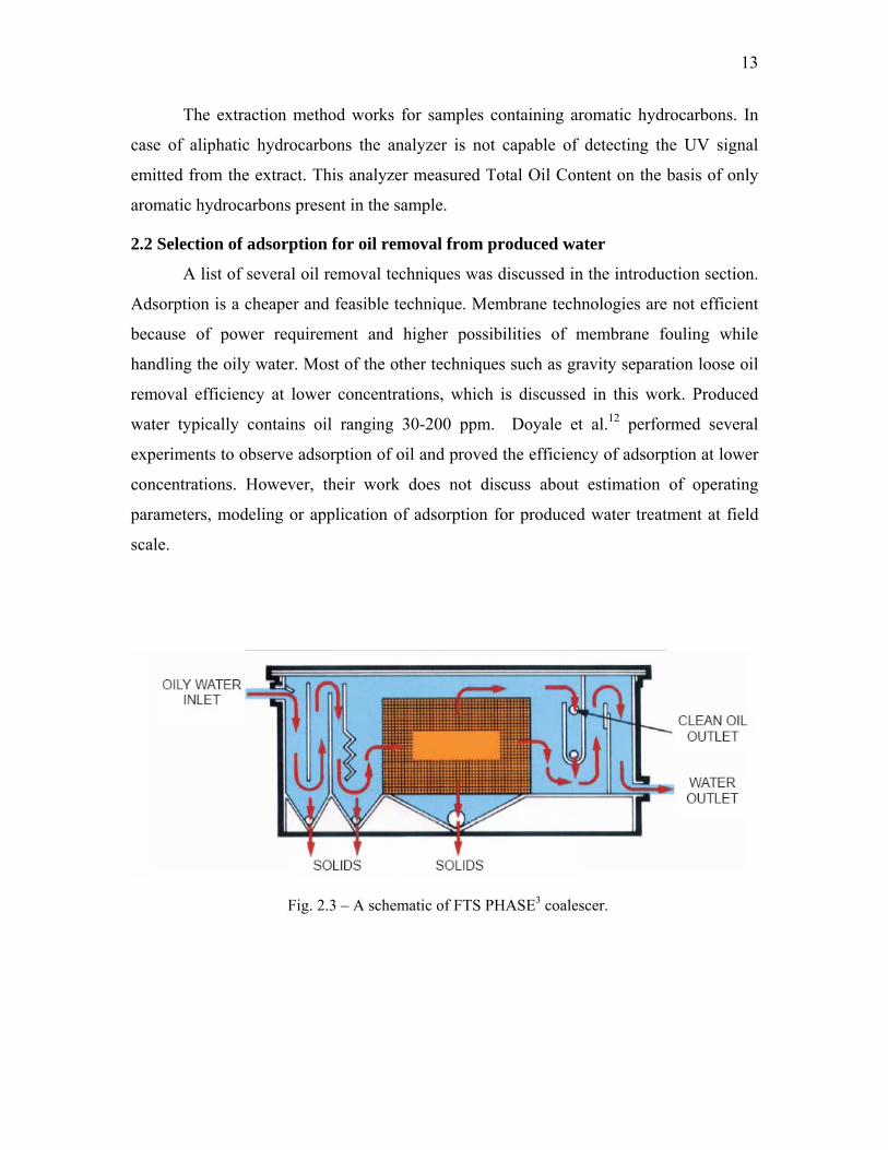
Fig. 2.3 – A schematic of FTS PHASE3 coalescer.

14

Several experiments were performed in this work to evaluate gravity separation

with FTS PHASE3 (Figure 2.3) oil-water separator.

The methods and the equipments to perform this operation have been improvised often.

For oil-water separation the use of the gravity separation method provide primary step

and require the back up treatment like filtration or adsorption.

Coalescer works on the principle of forming larger oil droplets which travel at

higher velocity and so the separation becomes rapid. A coalescing pack attracts oil

droplets which form larger droplets that rise quickly and thus produce faster phase

separation.

Oil-water separator should provide optimum efficiency in gravity separation

between two immiscible liquid fractions depending on initial oil content. The horizontal

orientation of the PHASE3 modules provides a uniform and non-clogging flow through

the coalescing tubes. The coalescing pack features a structured polypropylene coalescing

medium made of screen tubes unitized in removable baskets. The rectangular openings in

its tubular construction allow for settling solids to pass through the coalescing medium.

The design versatility of the PHASE3 also eliminates the staging that is necessary with

other incline and horizontal coalescing plates.

The FTS PHASE3 oil-water separator is of a gravity accelerator design with

coalescing slotted tube arrangements for processing both high oil and high solids content.

The inlet baffles reduce the oil-water mixture feed to laminar flow. The liquid then enters

the coalescing tubes under laminar conditions. According to Stoke’s law, rise and fall

velocity of dispersed phase droplet is exponentially increased with the droplet size. The

oleophilic surfaces of the coalescing tubes attract small oil droplets which in turn,

combine to form larger droplets for easier flotation. The oil rises to a collection point

while the water continues through the medium to the water outlets. Some of the attracting

features of this equipment are,

1. No pretreatment required.

2. High efficiency separation due to high surface area coalescing medium.

3. No moving parts

15

4. Easy cleaning; minimal maintenance.

5. All steel vessel construction.

6. Large solids settling area helps removing solids effectively if present in feed.

y = 141.39x2 - 88.525x + 426.49R2 = 0.9954

y = 30.53x2 + 156.75x + 195.8R2 = 0.9993

0

200

400

600

800

1000

1200

1400

1600

1800

0 1 2 3 4Feed flow, L/min

Out

let C

once

ntra

tion,

ppm

950 ppm 1900 ppm 3800 ppm 7600 ppmPoly. (7600 ppm) Poly. (3800 ppm)

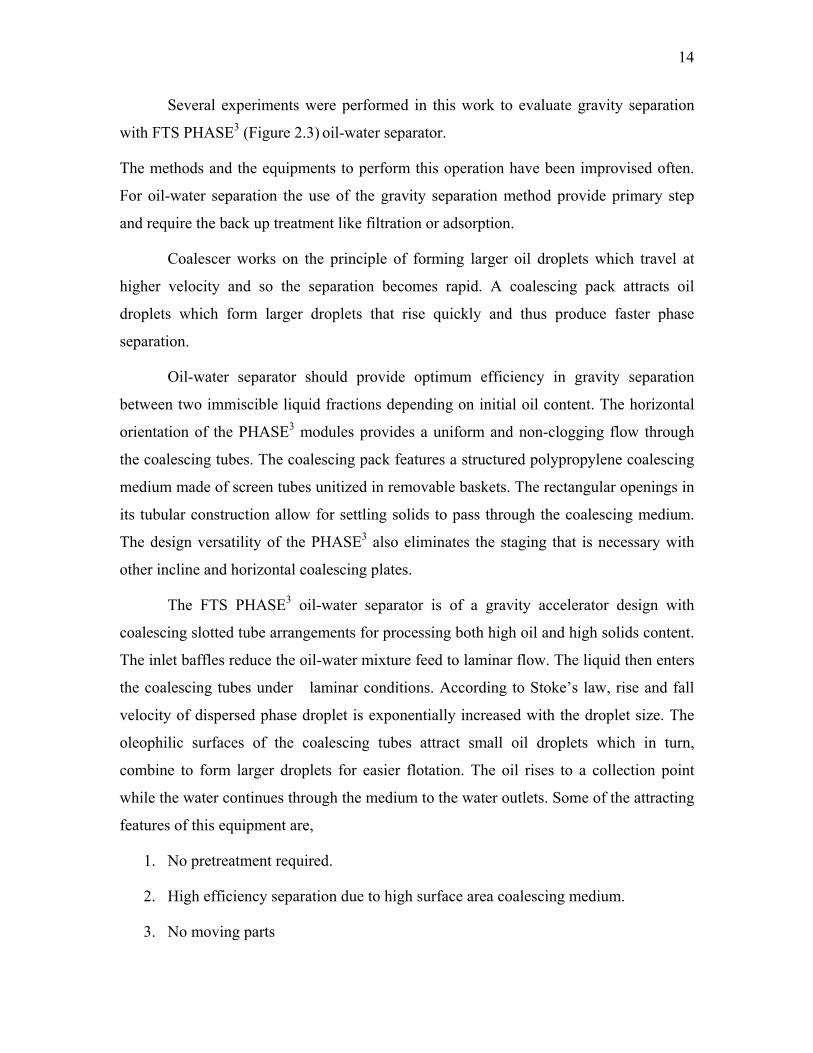
Fig. 2.4 – Effects of feed concentration and residence time on oil content of outlet from coalescer.

Coalescence efficiency is defined as the ratio of the outlet concentration to that of

the feed. Figure 2.4 shows that as the feed flow rate increases the coalescence time

decreases and so the outlet concentration increases. Figure 2.5 shows the coalescence

16

efficiency decreases as the inlet concentration and residence or coalescence time

decreases (increasing flow rate).

The use of a coalescer in produced water treatment is restricted because the

concentration of the produced water ranges from 30-200 ppm. The efficiency would be

much lower at this range and the outlet concentration might not be decreased down to 20-

30 ppm limit as required by EPA.

70

80

90

100

0 1 2 3 4Feed flow, L/min

Coa

lesc

ence

effi

cien

cy, %

950 ppm 1900 ppm 3800 ppm 7600 ppm

Fig. 2.5 – Effects of feed concentrations and residence time on oil removal efficiency of coalescer.

However, it might be effective and economical for suspended solids separation

from the produced water which is necessary to perform before oil removal by adsorption.

17

To evaluate removal of oil by adsorption several experiments were performed.

The analysis of results was accomplished by measuring TOC with TOC-700 and TD-500

analyzer. The next section discusses basic adsorption terminologies.

2.3 Adsorption terminologies

Loading Capacity or Adsorption Capacity (n):

It is the maximum amount of solute present in the liquid phase that can be

adsorbed by adsorbent. It can be defined as gm of oil or solute adsorbed per gm of

adsorbent.

Residence Time or Empty Bed Contact Time (EBCT):

Since the liquid flows through the pore space within adsorbent media residence

time is the time for which liquid phase containing adsorbate (solute to be adsorbed)

remains within the pore space in the packed bed.

The EBCT is defined as the time for which the liquid phase remains in the bed

which is not packed.

Q

LAEBCT cs==θ …………………………………………………………….(2.1)

……………………………………………………………..(2.2) ε= )()( EBCTRT

where, ε = porosity of the packed bed

RT = residence time, [t]

θ = empty bed contact time, [t]

Acs = cross sectional area of packed bed, [L]2

Q = volumetric flow rate through the packed bed, [L]3[t]-1

Bulk Density (ρb):

The bed or bulk density is the mass of adsorbent in a specific volume. It is a

measure of the amount of adsorbent that can be packed in a column of given volume.

18

Particle Density (ρp):

Particle density is the mass of adsorbent per volume occupied by the particle. This

is accurately and easily measured for true cylindrical pellets and beads, but is more

difficult for distorted shapes and granular materials, though proprietary methods exist for

obtaining accurate values even for those.

Solid Density (ρs):

Solid density is the mass of the adsorbent per volume occupied by the particle, but

with the pores deducted.

Isotherm:

Adsorption equilibrium data are commonly gathered at a fixed temperature and

plotted or tabulated as loading capacity or adsorption capacity of adsorbent versus the

fluid-phase concentration (or partial pressure for gases and vapors).

The simplest equilibrium isotherm expresses loading as proportional to the fluid-phase

concentration, and this results in Henry’s law.

………………………………………………………………………(2.3) Ac*q =

where, = equilibrium solute concentration in adsorbent, gm of oil/gm of adsorbent *q

c = solute concentration in liquid phase that is contacted to adsorbent, ppm

A = Henry’s law coefficient

In contrast, the Langmuir isotherm accounts for surface-coverage. That is, when

the fluid concentration is very high, a monolayer forms on the adsorbent surface. For

some systems, the apparent level of saturation may represent multiple adsorbed layers.

The parameter, A, is referred to as the Henry’s law coefficient, since it is the slope of the

isotherm at zero coverage.

Bc1

Ac*q+

= …………………………………………………………………..(2.4)

The Freundlich isotherm is the result of fitting isotherm data to a linear equation

on log-log coordinates. It is probably the most commonly used isotherm equation, despite

19

being “thermodynamically inconsistent,” in that it does not have a finite Henry’s law

coefficient.

BAc*q = …………………………………………………………………….(2.5)

Several other forms of isotherms have been discussed in detail in available

literature.

Adsorption Rate:

The rate of adsorption onto an adsorbent surface can be expressed as,

………………………………………………………………….(2.6) knads kcR =

where, Rads = adsorption rate

k = adsorption rate constant, [T]-1

nk = kinetic order coefficient

2.4 Evaluation of new organoclay adsorbent for oil removal

Produced water can be used as a source of fresh water after the oil content in

produced water is removed below 30 ppm according to EPA standards. Adsorption of oil

contents with organoclay bed is an economical method and the objective of this project is

to evaluate the performance of organoclay bed.

PS 12385 is a modified organoclay mineral manufactured by Polymer Venture

Inc. PS 12385 does not swell or blind when adsorbing contaminants, so it need not be

blended with anthracite filter. Table 2.1 indicates physical properties of PS12385.

The adsorption depends on various parameters such as organoclay weight,

porosity of bed, residence time in the bed, feed concentration and bed preparation

techniques.

20

TABLE 2.1 – Properties of proposed new adsorbent organoclay PS18385 for oil removal from produced water. Appearance Gray to Tan Granules

Specific Gravity 2.0 – 2.2

Bulk Density 42 – 46 lbm/ft3

Granule Size 8/30 mesh (US sieve, Average opening 1.6 mm)

Residence Time 2 – 4 min

Void Volume 35 – 45%

One of the analysis methods is the breakthrough curve. Breakthrough curve is the

plot of outlet concentrations from packed bed vs. time. Obtaining breakthrough curve for

each experiment and comparing these curves to do parametric analysis is one of the

objectives of the project.

2.4.1 Packed bed adsorption experiments

To analyze the performance of organoclay bed several experiments are

performed. Since it is necessary to achieve breakthrough of packed bed to analyze

adsorption capacity and kinetics, highly concentrated influent are required. Experiments

were performed with highly concentrated kerosene-water emulsions and crude oil-water

emulsions. Several combinations of feed concentration, residence time and particle size

distribution were used to evaluate the effects of these parameters on adsorption.

Methodology and procedure

The bed is packed to ensure minimum channeling and soaked with the feed water

to wet the organoclay particles. The flowchart of experiment is given below in Figure 2.6.

To maintain lower flow rate feed is recycled to feed tank in some experiments.

21

By Pass Outlet

Column Feed

Stirrer

Fig. 2.6 - A schematic of experimental setup for adsorption operation.

To analyze kinetics of adsorption, effect of bed dynamics and loading capacity of

adsorbent, it is necessary to achieve breakthrough curve for each experiment. The packed

bed dimension, weight of organoclay, feed concentration, breakthrough time and

residence time must be estimated before starting the experiment.

The EBCT suggested by the manufacturer is 3 to 6 min. The dimensions of the

column are fixed on the basis of the amount of organoclay to be used. For same diameter

column different amount of organoclay would give different Length of Column to

Diameter of column ratio. The flow rate through the column is determined after

measuring the porosity of the packed bed. The flow rate is adjusted to obtain EBCT value

as low as 3 min. To maintain such low flow rate through the column for as long as

experiment run with the available pump is accomplished by providing a by pass and

controlling the flow by valves. The adsorbent is the material that is used in adsorption

column as the filtering media. It must adsorb wide range of hydrocarbons and trace

amount of heavy metals from produced water.

The pore network on the surface of the particles is clearly seen in Scanning

Electron Microscopic (SEM) image (figure 2.7). Figure 2.8 clearly indicate the presence

of diatoms in abundance. Diatoms are skeletons of dead micro organisms which are very

porous in nature.

22

Fig. 2.7 – SEM image of un-crushed organoclay particle.

Pore Network

Fig. 2.8 – Diatoms provide porous structure to organoclay.

To minimize channeling and wall effects in a packed column the ratio of diameter

of the column to the diameter of adsorbent should be within 30-6020. To achieve the ratio

23

within this range in laboratory the organoclay particles were crushed and sieved (figure

2.9) before packing.

An advantage of size reduction of organoclay is the increase in fluid-to-particle

mass transfer coefficient. Also size reduction increases the surface area of the particles

and hence the fluid-solid contact area (adsorption area). It can be observed that for a

given flow rate, reduction in particle size would increase mass transfer coefficient. Also

increase in velocity would increase in mass transfer coefficient but it is obvious that as

the velocity of fluid through the column increases the contact time or the residence time

decreases which results into less time for adsorption and so lower loading capacity.

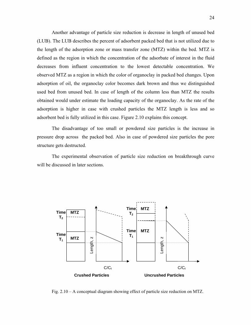
The conceptual difference in breakthrough curve under same operating conditions

i.e. residence time, inlet concentration, porosity for different particle sizes is the

difference in sharpness of the curve. In case of reduced or crushed particles the

breakthrough curve is steeper because of faster adsorption kinetics, while for uncrushed

particles the breakthrough curve is distended.

0.7112 mm opening

1.19 mm opening

Fig. 2.9 – Reduction of size of organoclay particle in laboratory.

24

Another advantage of particle size reduction is decrease in length of unused bed

(LUB). The LUB describes the percent of adsorbent packed bed that is not utilized due to

the length of the adsorption zone or mass transfer zone (MTZ) within the bed. MTZ is

defined as the region in which the concentration of the adsorbate of interest in the fluid

decreases from influent concentration to the lowest detectable concentration. We

observed MTZ as a region in which the color of organoclay in packed bed changes. Upon

adsorption of oil, the organoclay color becomes dark brown and thus we distinguished

used bed from unused bed. In case of length of the column less than MTZ the results

obtained would under estimate the loading capacity of the organoclay. As the rate of the

adsorption is higher in case with crushed particles the MTZ length is less and so

adsorbent bed is fully utilized in this case. Figure 2.10 explains this concept.

The disadvantage of too small or powdered size particles is the increase in

pressure drop across the packed bed. Also in case of powdered size particles the pore

structure gets destructed.

The experimental observation of particle size reduction on breakthrough curve

will be discussed in later sections.

Fig. 2.10 – A conceptual diagram showing effect of particle size reduction on MTZ.

Leng

th, z

Leng

th, z

C/CfC/Cf

MTZ

MTZ Time

T1

TimeT1

Time MTZ Time MTZ T2

T2

Crushed Particles Uncrushed Particles

25

2.5 Data acquisition and presentation

The packed bed porosity was measured before starting an experiment. The packed

bed is filled with water to hold maximum amount of water. The weight of water filled

packed bed, organoclay and empty columns were measured accurately.

The weight of water that organoclay bed holds is,

…………………………………………………...(2.7) cWocWpackedWW −−=

where, WOC = weight of organoclay packed within the column, gm

WC = weight of unpacked column, gm

Volume of water is,

…………………………………………………………..(2.8) WwaterwaterV ρ=

We also have the volume of column (Voc) that is packed with organoclay, which is

obtained by multiplying the cross sectional area of unpacked column (diameter of column

is known) with the height of the packed column.

The porosity of the bed is,

ocV

waterV=ε …………………………………………………………………...(2.9)

For each experiment breakthrough was achieved. The breakthrough curve is the

plot of packed bed outlet concentration vs. time. For each experiment outlet samples were

collected and analyzed to measure TOC by TOC-700 or TD-500 analyzer. Average

residence time and pore volume processed before the breakthrough was calculated.

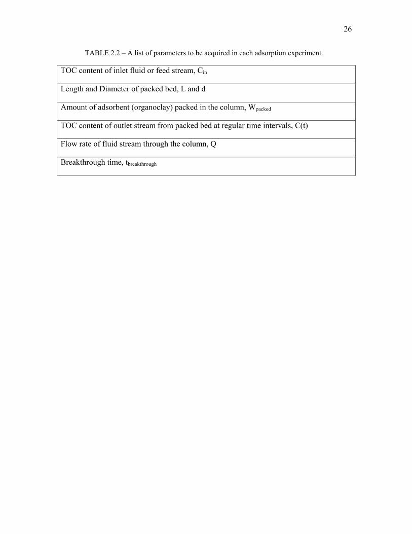
Adsorption capacity was determined by performing material balance calculations. Table

2.2 shows the list of data acquired when performing adsorption experiments.

26

TABLE 2.2 – A list of parameters to be acquired in each adsorption experiment.

TOC content of inlet fluid or feed stream, Cin

Length and Diameter of packed bed, L and d

Amount of adsorbent (organoclay) packed in the column, Wpacked

TOC content of outlet stream from packed bed at regular time intervals, C(t)

Flow rate of fluid stream through the column, Q

Breakthrough time, tbreakthrough

27

CHAPTER III

DISSOLVED SOLID REMOVAL FROM PRODUCED WATER

3.1 Selection of reverse osmosis (RO)

Reverse osmosis is capable of rejecting bacteria, salts, sugars, proteins, particles,

dyes, and other constituents that have a molecular weight of greater than 150-250

Daltons. The separation of ions with reverse osmosis is aided by charged particles. This

means that dissolved ions that carry a charge, such as salts, are more likely to be rejected

by the membrane than those that are not charged, such as organics. The larger the charge

and the larger the particle, the more likely it will be rejected. One of the factors for

selecting RO over other membrane filtration processes such as Micro-filtration (MF),

Ultra-filtration (UF) etc. is that mono-valent salt can not pass through RO membrane. RO

can remove salt particles which can not be removed by MF or UF membranes.

The idea of RO is to use the membrane to act like an extremely fine filter to create

drinkable water from salty (or otherwise contaminated) water. Osmosis is the movement

of a solvent through a semi permeable membrane into a solution of higher solute

concentration that tends to equalize the concentrations of solute on the two sides of the

membrane. In RO, the salty water passes through on one side of the membrane and

pressure is applied to stop, and then reverse, the osmotic process.

Reverse osmosis uses a membrane that is semi-permeable, allowing the fluid that

is being purified to pass through it, while rejecting the contaminants that remain. Most

reverse osmosis technology uses a process known as cross-flow to allow the membrane to

continually clean itself. As some of the fluid passes through the membrane the rest

continues downstream, sweeping the rejected species away from the membrane. The

process of reverse osmosis requires a driving force to push the fluid through the

membrane, and the most common force is pressure from a pump. The higher the pressure,

the larger the driving forces. As the concentration of the fluid being rejected increases,

the driving force required to continue concentrating the fluid increases. This pressure

must exceed the osmotic pressure of the feed solution.

28

Siddiqui14 performed several RO experiments to evaluate its application for

removing dissolved solids from the produced water and proved RO as the best and the

most efficient technique for this particular application. Though Siddiqui14’s work

discusses economical analysis of RO, it does not discuss modeling and up-scaling of RO

for field scale application.

In this thesis, RO experiments were performed to duplicate Siddiqui14’s results

and based on experimental data an empirical model is developed. The modeling and

simulation of RO is discussed in later sections.

3.2 RO terminologies

Figure 3.1 shows a schematic of spiral wound RO membrane. The feed is passed

through the membrane via feed spacer with cross-flow configuration. Only pure water

present in the feed can pass through the semi permeable membrane leaving concentrated

or salty water behind which eventually is collected as concentrate. Permeate is collected

at the end of the perforated product line passes through the membrane. The transport of

pure water from feed side to permeate side depends on the trans-membrane pressure

across the RO unit, the feed flow rate and area of the membrane. To reduce the

dimensionality of the RO designing problem we can define flux as the ratio of flow to the

area.

Feed

Permeate

Concentrate

Fig. 3.1 – Schematic of spiral wound RO membrane in operations.

29

Trans-membrane pressure:

It is defined as the average pressure applied across the membrane minus the

pressure on the permeate side.

pPoPiPP −

+=

2∆ …………………………………………………………...(3.1)

where,

Pi = pressure at the feed inlet side, psi

Po = pressure at the concentrate outlet side, psi

Pp = pressure at the permeate outlet side, psi

Permeate recovery:

Permeate recovery = permeate flow rate/feed flow rate ……………………...(3.2)

Salt rejection:

Salt rejection represents the percentage of salt that can be removed form the feed.

Salt rejection = 1-Cperm/Ctds…………...............………………………………(3.3)

where,

Cperm = salt concentration in permeate, ppm

Ctds = average salt concentration in feed, ppm

Higher salt rejection and higher permeate recovery represents better purification

of water using RO membrane. Optimum trans-membrane pressure should be determined

to perform economic RO operations.

3.3 Experimental setup

A standard commercial 4X40 membrane (4 inch Diameter and 40 inch Length)

was used for the experiments with produced water having TDS ranging from 10000-

40000 ppm. The surface area provided by spiral membrane is 70 ft2. Temperature has an

effect on the trans-membrane pressure to be applied across the RO membrane. As the

temperature increases the osmotic pressure increases, which requires higher trans-

membrane pressure to get desired salt removal keeping all the other parameters

30

unchanged. Also as the temperature increases the viscosity decreases, which somewhat

lowers the demand of trans-membrane pressure. So there is an offsetting effect of

increase in temperature. In our experiments we kept the temperature constant at 350C

The performance of the RO unit with a particular type of membrane, determined

in terms of permeate recovery fraction, permeate flux, permeate concentration and salt

rejection depend on the concentration (salinity) of the feed, feed flow rate through the RO

unit and the applied trans-membrane pressure. Figure 3.2 shows a RO unit that was

utilized to perform the experiments.

The feed was prepared using NaCl-water solution. The osmotic pressure of NaCl

is higher than that is of various salts those may present in the produced water. The trans-

membrane pressure required to remove NaCl salt from water would be higher that that is

required in the case of other salts. For example if a trans-membrane pressure of 800 psi

removes 90% NaCl salt from water then it would remove more than 90% of other salts

such as barium, calcium salts etc. The result of the experiments performed with NaCl-

water solution conservatively determines range of operating parameters.

Fig. 3.2 – Laboratory unit to perform pilot scale RO operations.

31

3.4 Data acquisition and presentation

First the experiments were performed with pure water as feed to determine

properties of membrane. If the clean water flux through the RO membrane is competitive,

the membrane should be further investigated with salty water. Flux is defined as the ratio

of flow rate to the membrane surface area. The content of TDS in each sample was

measured by conductivity meter. The RO membrane was tested with feed having salt

concentration upto10000-40000 ppm.

The following parameters were measured at regular time interval,

• Trans-membrane pressure

• Feed flow rate

• Permeate flow rate

• Concentrate flow rate

• Feed concentration

• Permeate concentration

• Salt content in concentrate side

These measurements provided a definite tool for modeling transient RO filtration

performance.

32

CHAPTER IV

RESULTS AND DISCUSSION

4.1 Packed bed adsorption

The study of packed bed adsorption is accomplished by analyzing breakthrough

behavior of packed bed. The breakthrough curve is a plot of outlet concentration vs.

operation time. It can also be plotted as the ratio of outlet concentration to the inlet

concentration vs. operation time. The adsorption is a two stage process.

Stage I: Diffusion of solute from bulk fluid phase to the surface of adsorbent particle. It

is controlled by molecular diffusion. In most cases resistance to molecular diffusion is

negligible.

Stage II: Adsorption or uptake of solute within the pore structure of adsorbent. It is

controlled by surface diffusion or pore diffusion or combination of both.

The sharpness of the breakthrough curve near the breakthrough region represents

adsorption kinetics. A sharper breakthrough curve indicates negligible resistance to the

uptake or adsorption of solute in the adsorbent.

The adsorption rate is affected by size of adsorbent particle and feed

concentration in isothermal operation. The adsorption capacity is affected by surface area

of adsorbent, porosity of adsorbent particle and packed bed, solubility and type of solute

in feed and EBCT.

To accomplish comprehensive analysis of oil adsorption by organoclay, the effect

of the above parameters on adsorption capacity and breakthrough curve was observed.

Loading capacity or adsorption capacity of packed bed can be calculated by performing

material balance over the experiment run time until the breakthrough is achieved.

4.1.1 Effect of contact time

As the contact time between oil in feed and the organoclay particles increases,

more amount of oil gets adsorbed within the pore structure of organoclay. Table 4.1

indicates that for experiments with approximately same concentration of kerosene in

water, adsorption capacity for the experiment with longer EBCT was approximately 15%

33

more. The EBCT used in experiment A was approximately 3.5 times higher than EBCT

used in experiment B.

It is interesting to observe the breakthrough curve for both experiments as it gives

a hint about adsorption kinetics. Figure 4.1 shows that at early times the outlet

concentrations for experiment B are higher than that of experiment A. For lower EBCT

the organoclay particles require more time to get wetted. This type of concentration

behavior indicates lower adsorption rate at early times when particles are in process of

getting wetted with the oil present in feed. Once, the particles are wetted they respond

more quickly and adsorption rate gets higher at large times. We soaked the column for

more than 24 hrs before operation. As it can be seen from the figure that the breakthrough

sharpness pattern is very much similar, this indicates minor effect of velocity of fluid

(inverse of EBCT) on the adsorption kinetics at higher concentrations. This phenomena is

important particularly in modeling point of view as the conclusion can be drawn based

upon this behavior that at early times pore diffusion controls the adsorption and at large

times film diffusion or combination of diffusions controls the adsorption.

TABLE 4.1 – Experiments with same feed concentration, particle size but different EBCT.

Experiment A B

Weight of organoclay packed, gm 25.00 20.00

Length of organoclay bed, cm 9.20 7.60

Volume of organoclay bed, cm3 39.04 32.25

Porosity of packed bed 0.38 0.38

Feed Concentration, ppm ≈ 7000 ≈ 7000

Average particle diameter, mm 0.95 0.95

Breakthrough time, min 275 212

EBCT, min 7.58 2.92

Average flow rate, ml/min 5.16 11.04

Adsorption capacity, gm oil / gm of organoclay 0.85 0.73

34

100

1000

10000

0 100 200 300 400Time, min

C(t)

, ppm

Exp.A, EBCT=7.58 minExp.B, EBCT=2.92 min

Fig. 4.1 – Comparison of breakthrough curve for experiments with different EBCT.

In either case, more than 90% of removal of oil is observed even with lesser

EBCT and higher feed concentration.

4.1.2 Effect of size of organoclay particle

Smaller particle sizes provide larger contact area available for adsorption and

consequently higher adsorption rate. Also it would be interesting to observe effect of

particle size reduction on adsorption capacity. The particle size should be small but if the

particles are in powdered form the porous structure of the particle would no longer be

suitable for adsorption, also the pressure drop would increase and clogging may occur.

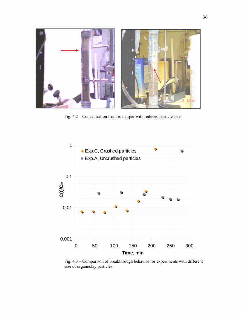
Table 4.2 shows parameters and results from two experiments with different

particle size. The results have a combined effect of different particle size and different

concentrations. The EBCT is approximately the same in both cases. The adsorption

kinetics is much higher with smaller particle size. In this case a sharper concentration

front was observed by noticing color change in a transparent column packed with

organoclay. Figure 4.2 shows the concentration front pattern for both experiments and

35

Figure 4.3 shows the breakthrough curves. The decrement in adsorption capacity can be

reasoned as a combined effect of increment in feed concentration and up to some extent

higher particle size.

TABLE 4.2 – Experiments with different feed concentration and particle sizes. Experiment C A





Feed concentration, ppm ≈13600 ≈ 7000



EBCT, min 8.16 7.48



36

Fig. 4.2 – Concentration front is sharper with reduced particle size.

0.001

0.01

0.1

1

0 50 100 150 200 250 300Time, min

C(t)

/Cin

Exp.C, Crushed particlesExp.A, Uncrushed particles

Fig. 4.3 – Comparison of breakthrough behavior for experiments with different size of organoclay particles.

37

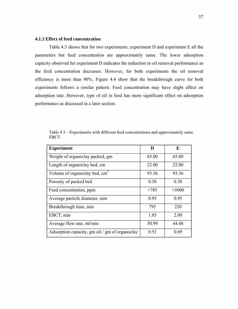
4.1.3 Effect of feed concentration

Table 4.3 shows that for two experiments, experiment D and experiment E all the

parameters but feed concentration are approximately same. The lower adsorption

capacity observed for experiment D indicates the reduction in oil removal performance as

the feed concentration decreases. However, for both experiments the oil removal

efficiency is more than 90%. Figure 4.4 show that the breakthrough curve for both

experiments follows a similar pattern. Feed concentration may have slight effect on

adsorption rate. However, type of oil in feed has more significant effect on adsorption

performance as discussed in a later section.

Table 4.3 – Experiments with different feed concentrations and approximately same EBCT. Experiment D E





Feed concentration, ppm ≈785 ≈5000



EBCT, min 1.85 2.09



38

0.01

0.1

1

10 100 1000

Time, min

C(t)

/Cin

Exp.D, 785 ppm

Exp.E, 5000 ppm

Fig. 4.4 – Comparison of breakthrough behavior for experiments with different feed concentrations.

Table 4.4 shows results obtained for an experiment with produced water as feed.

The inlet is oil field produced water having TOC of approximately 59 ppm. The EBCT of

6 min is used to accomplish oil removal. The results indicate approximately 80% oil

removal by packed bed adsorption operation.

39

Table 4.4 – Experimental results with produced water as feed. The column had not received the breakthrough (sharp increase in concentration is not observed).

Time

Min

Outlet Concentration

ppm

20 12.90

45 11.64

60 13.20

120 13.00

160 12.26

250 13.12

0

10

20

30

40

50

60

70

0 50 100 150 200 250 300Time, min

Out

let T

OC

, ppm

Outlet concentrationFeed concnetration

Fig. 4.5 – Results for an experiment with produced water as feed.

40

Figure 4.5 represents data for the experiment that has not yet achieved the

breakthrough. Obviously, as EBCT increases the percentage of adsorption would also

increase as discussed earlier. The underperformance of the packed bed can be justified by

the fact that the produced water contains trace amount of suspended solids, salts,

microorganisms and other impurities. Alternately, using packed bed adsorption columns

in series facilitates lesser EBCT or higher throughput operation. The outlet from first

packed bed adsorption column can be used as feed for the second column. The number of

columns to be configured is series depends on feed concentration and desired outlet

concentrations.

4.1.4 Effect of type of oils

Table 4.5 shows the comparison of experimental parameters and results for

experiments with kerosene-water emulsions and crude oil-water emulsions. Experiment F

is for a crude oil-water emulsion while experiment G is for a kerosene-water emulsion is

used as feed.

TABLE 4.5 – Experimental parameters for experiments with different types of oil present in feed. Experiment F G





Feed concentration, ppm 1650 8495



EBCT, min 6.20 3



Type of oil content in feed crude oil kerosene

41

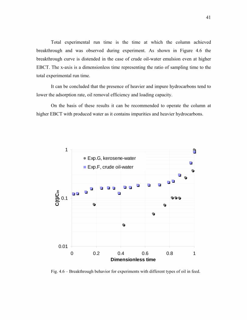
Total experimental run time is the time at which the column achieved

breakthrough and was observed during experiment. As shown in Figure 4.6 the

breakthrough curve is distended in the case of crude oil-water emulsion even at higher

EBCT. The x-axis is a dimensionless time representing the ratio of sampling time to the

total experimental run time.

It can be concluded that the presence of heavier and impure hydrocarbons tend to

lower the adsorption rate, oil removal efficiency and loading capacity.

On the basis of these results it can be recommended to operate the column at

higher EBCT with produced water as it contains impurities and heavier hydrocarbons.

0.01

0.1

1

0 0.2 0.4 0.6 0.8 1Dimensionless time

C(t)

/Cin

Exp.G, kerosene-water

Exp.F, crude oil-water

Fig. 4.6 – Breakthrough behavior for experiments with different types of oil in feed.

42

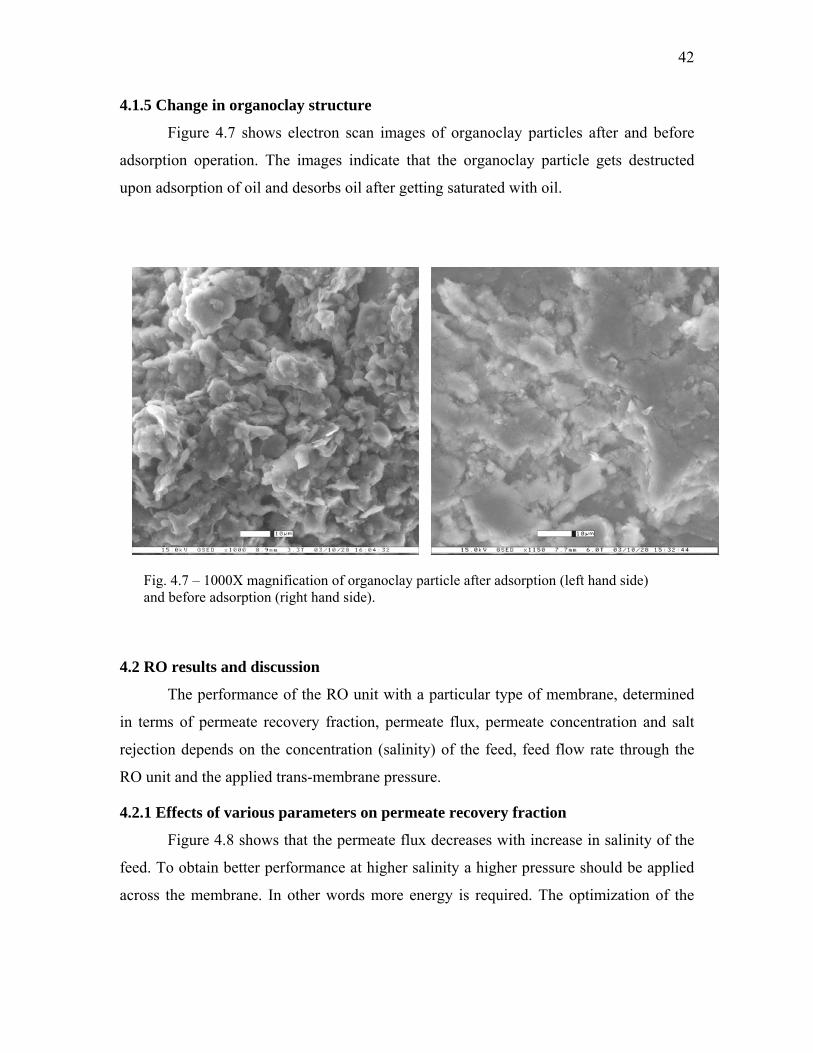
4.1.5 Change in organoclay structure

Figure 4.7 shows electron scan images of organoclay particles after and before

adsorption operation. The images indicate that the organoclay particle gets destructed

upon adsorption of oil and desorbs oil after getting saturated with oil.

Fig. 4.7 – 1000X magnification of organoclay particle after adsorption (left hand side) and before adsorption (right hand side).

4.2 RO results and discussion

The performance of the RO unit with a particular type of membrane, determined

in terms of permeate recovery fraction, permeate flux, permeate concentration and salt

rejection depends on the concentration (salinity) of the feed, feed flow rate through the

RO unit and the applied trans-membrane pressure.

4.2.1 Effects of various parameters on permeate recovery fraction

Figure 4.8 shows that the permeate flux decreases with increase in salinity of the

feed. To obtain better performance at higher salinity a higher pressure should be applied

across the membrane. In other words more energy is required. The optimization of the

43

RO parameters for a particular type of feed is the maximum permeate recovery at the

minimum energy requirement.

0

5

10

15

20

25

30

0 200 400 600 800 1000Transmembrane pressure, psi

Perm

eate

Flu

x, G

allo

n/ft2 /D

ay

6 gpm-10000 ppm 8 gpm-10000 ppm 10 gpm-10000 ppm6 gpm-20000 ppm 8 gpm-20000 ppm 10 gpm-20000 ppm

Fig. 4.8 – Effects of TDS content and flow rate of feed on permeate flux at various transmembrane pressure.

Figure 4.9 shows that the permeate recovery is higher for lower salinity feed for

all the feed flow rates compared to higher salinity feed. Also for a particular salinity feed

the permeate recovery increases as the feed flow rate decreases. At higher feed flow rate

to get better performance more pressure should be applied across the membrane.

44

0.00

0.05

0.10

0.15

0.20

0.25

0 200 400 600 800 1000

Transmembrane pressure, psi

Perm

eate

reco

very

frac

tion


Fig. 4.9 – Effects of TDS content and flow rate of feed on permeate recovery fraction at various transmembrane pressure.

4.2.2 Effects of various parameters on salt removal

Figure 4.10 and Figure 4.11 shows the permeate concentration and the salt

rejection respectively for different salinity feed at different flow rates and trans-

membrane pressures.

For a particular salinity feed at a particular feed flow rate the salt rejection

increases as the trans-membrane pressure increases up to a certain limit after which the

salt rejection remains the same even if the trans membrane pressure increases. The

experimental permeate concentration and salt rejection data can be expressed by a second

order polynomial equation. Such models would be limited for only one set of feed

salinity or trans-membrane pressure. The development of a general empirical model that

incorporates all sets of feed salinity, trans-membrane pressure and flux is discussed in

next chapter.

45

94.595

95.596

96.597

97.598

98.599

99.5


Salt

Rej

ectio

n, %

8 gpm-10000 ppm 10 gpm-10000 ppm 8 gpm-20000 ppm10 gpm-20000 ppm 8 gpm-30000ppm 10 gpm-30000ppm

Fig. 4.10 – Effects of TDS content and flow rate of feed on salt rejection at various transmembrane pressure.

The permeate concentration can be obtained as low as 30 ppm with RO units for

produced water up to 40000 ppm TDS. The configuration of two or more RO units in

series can be helpful in further lowering permeate (outlet) concentration.

46

050

100150200250300350400450


Perm

eate

Con

cent

ratio

n, p

pm


Fig. 4.11 – Effects of TDS content and flow rate of feed on permeate concentration at various transmembrane pressures.

47

CHAPTER V

MODELING AND SIMULATION

5.1 Literature review

,

Adsorbent Particle

Liquid Film

CbCavg

.qavg.

Cs

Fig. 5.1 – A schematic diagram of packed bed adsorption column.

The packed bed adsorption process can be described as a stage wise process

(figure 5.1). The solute (oil particles in our case) present in the bulk liquid phase first

migrates through to the surface of the adsorbent particle. Adsorbent particle can be

visualized as having a stagnant liquid film surrounding it. Transfer of solute through this

film can only occur by molecular diffusion. If it is a slow process then in most of the

packed bed adsorption it is the process that controls adsorption rate. If it is faster then the

concentration at the surface of the adsorbent particle, Cs, is same as the concentration in

bulk phase, Cb. The resistance offered by liquid film is termed as external mass transfer

resistance.

48

In next stage, the solute on the surface of the adsorbent particle migrate through

the porous structure of the adsorbent particle and attach itself in a vacant site. The

resistance offered by this step is termed as internal mass transfer resistance. The mass

transfer of solute from the surface in to the adsorbent can be described by two

mechanism, pore diffusion and surface diffusion. Surface diffusion is the diffusion of

solute along the surface of the adsorbent particle and pore diffusion is the diffusion of

solute within the pore structure of solid itself.

The rate at which the solute particle from bulk fluid phase is transported through

and adsorbed on to the porous structure of adsorbent particle is referred as solute uptake

rate or adsorption rate. Several uptake rate models and associated assumptions have been

discussed in the literature17 - 25.

The differential mass balance equations of solute in a packed bed can be written

in the following form. To make the model simpler the axial dispersion is neglected,

which is an excellent assumption in case of liquid flow through the packed bed.

( ) 0aRtcvc

z=+

∂∂

+∂∂ …………………………………………………………(5.1)

where, v = interstitial velocity of fluid within packed bed, cm/min or inch/min

z = length of packed bed, [L]1

t = time of operation, [t]1

c = concentration of solute in fluid phase changing with z and t, ppm

Ra = overall adsorption rate, [t]-1

The adsorption rate equation comprises of one or more diffusion mechanism

(molecular diffusion, surface diffusion and pore diffusion) with associated boundary

conditions, incorporating equilibrium constraints to which the mass transfer rate or

adsorption rate expression must reduce at sufficiently long times.

Analytical expressions for overall adsorption rate are available in literature. These

expressions involve different types of diffusion control mechanism and isotherms.

49

For example, Crank’s19, 20 solution considers adsorbent surface diffusion control

mechanism and a linear isotherm. Thomas 19, 20 developed a general model for Langmuir

isotherm that can be applied to any order of driving force considering film diffusion or

molecular diffusion mechanism. Glueckauf20 developed LDF (Linear Driving Force)

model for pore diffusion and surface diffusion that can be applied to any isotherm. Yao

and Tien22 developed approximate uptake rate expression that can be solved using

numerical techniques.

The mass balance differential equation and the linear isotherm and LDF rate law

were solved by Beaton and Furnas23. The expression is valid for the case of a uniform

feed concentration to an initially solute-free adsorbent.

),(JCC

in

τξ= …………………………………………………………………(5.2)

where, ξ = a dimensionless distance

τ = a dimensionless time

( v/kZ )εξ = …………………………………………………………………..(5.3)

[ ] ([ v/Zt)(K/k −−= )]ετ 1 …………………………………………………..(5.4)

where, k = uptake rate kinetics, [t]-1

K = linear isotherm constant, gm oil adsorbed/gm adsorbent/ppm

Z = length of packed bed, [L]

v = interstitial velocity of fluid in packed bed, [L][t]-1

∫ ∂−−−=ξ

ξτξτξτξ0

0 21 )(I)exp(),(J ……………………………………...(5.5)

where, I0 = hyperbolic zero-order Bessel function of first kind

Thomas19, 20 provided an expression for LDF rate law and Langmuir isotherm

system using the J function.

50

Rice20 proved that the J function provides exact solution for systems that can be

characterized by a combination of molecular diffusion and solid-phase diffusion (surface

diffusion or pore diffusion).

To solve a breakthrough behavior using analytical solution, through knowledge of

driving force law, type of isotherm and controlling mechanism is required. In our case the

experimental results do not provide sufficient information which is required to obtain

analytical solution.

If the all of the mass transfer resistances are too small, breakthrough font

approaches as a step change or a shock wave through the packed bed.

The experiments performed with kerosene-water emulsion as feed exhibited same

breakthrough behavior. The resistances offered by adsorbent particles to the kerosene

molecules were negligible. The step behavior of breakthrough curve can be modeled

easily by solving for solute material balance.

An alternate approach is to develop an empirical model for uptake rate that can be

applied to any isotherm form. The concept assumes that the transition of concentration

form the initial to that of feed is due to mass transfer resistance only. The empirical

model doesn’t take into account the isotherm expression and constants, this facts makes

its application limited to estimate rate constant and not the percentage of adsorption. The

Wheeler – Robell19, 20 equation is an empirically corrected local equilibrium model. Like

other simple models it neglects axial dispersion. Unlike most other equation-based

models, however, it applies to any isotherm form. Finally, assuming first order adsorption

the empirical equation can be written as,

( )

⎥⎦

⎤⎢⎣

⎡⎟⎟⎠

⎞⎜⎜⎝

⎛−=

== LAt

nQC

Qkexp

ctL,zcC cs

b

inw

ind ρ ……………………….(5.6)

In above equation if we choose outlet concentration equals to the inlet

concentration and solve the equation for time the resultant time is referred as

stoichiometric time.

51

nQCLAt

bin

css ρ= ……………………………………………………………...(5.7)

where, ρb = bulk density of packed bed, gm of adsorbent/volume of packed bed

Q = volumetric flow rate through the column, [L]3[t]-1

Acs = cross-sectional area of empty bed, [L]2

kw = adsorption rate coefficient, [t]-1

n = adsorption capacity or loading capacity, gm oil/gm of adsorbent

L = length of the packed column, [L]

The values of adjustable parameters kw and n depend on operating parameters

such as feed concentration, particle size, column length to diameter ratio and amount of

adsorbent being used.

To determine these parameters, the breakthrough data for each experiment is

fitted to above equation using non-linear regression code in Mathematica. It utilizes

Levenberg-Marquardt algorithm. Figure 5.2 shows an example of fitting of empirical

model to the experimental data obtained for the experiment with crude oil in water

(experiment G). The adjusting parameters were obtained for each experiment. The

empirical model fits well with the experimental results near breakthrough region. It

matches the sharp breakthrough curve pattern at large times. However, the model fits

poorly with experimental data at the beginning of the experiment and early times data

because of the exponential nature of the model. The model is fair enough to estimate and

analyze uptake or adsorption kinetics. The fitting model parameters were,

kw = 0.66 min-1

n = 0.54 gm oil adsorbed/ gm of organoclay

52

0.00.1

0.20.3

0.40.50.6

0.70.8

0.91.0

0 500 1000 1500

Time, min

C(t)

/Cin

Experimental data Empirical model

Fig. 5.2 – Fitting an empirical model to the breakthrough data for experiment G.

The use of analytical models and empirical models are limited because of lack of

isotherm data and knowledge of uptake rate mechanism. In the next section, a hybrid

approach to match breakthrough behavior is discussed.

5.2 A new approach for modeling of adsorption

The idea is to fit the data from the experiment in which the feed is crude oil and

water mixture. Fitting the ration of amount of oil adsorbed per unit of amount of oil

charged at various times. The ratio of instantaneous amount of oil adsorbed to the

instantaneous amount of oil inflow to the packed column exhibits a hyperbolic behavior

with respect to time axis. The time axis is taken as the ratio of time to the stoichiometric

time to make the time axis dimensionless. The expression for this approach would be,

)b/(tricstoichiome

ads

in

ads

))t/t(bD(m

WW

11+= …………………………………………..(5.8)

where, Wads = instantaneous amount of oil adsorbed in packed bed, gm

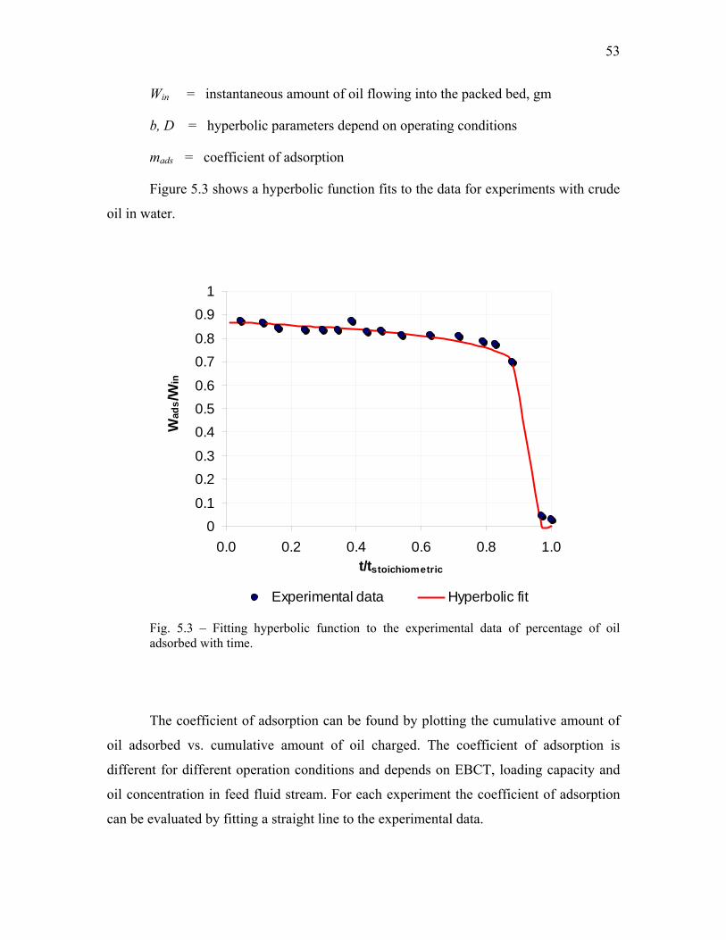
53

Win = instantaneous amount of oil flowing into the packed bed, gm

b, D = hyperbolic parameters depend on operating conditions

mads = coefficient of adsorption

Figure 5.3 shows a hyperbolic function fits to the data for experiments with crude

oil in water.

00.1

0.20.3

0.40.50.6

0.70.8

0.91

0.0 0.2 0.4 0.6 0.8 1.0t/tstoichiometric

Wad

s/Win

Experimental data Hyperbolic fit

Fig. 5.3 – Fitting hyperbolic function to the experimental data of percentage of oil adsorbed with time.

The coefficient of adsorption can be found by plotting the cumulative amount of

oil adsorbed vs. cumulative amount of oil charged. The coefficient of adsorption is

different for different operation conditions and depends on EBCT, loading capacity and

oil concentration in feed fluid stream. For each experiment the coefficient of adsorption

can be evaluated by fitting a straight line to the experimental data.

54

Oil adsorbed = 0.9729 Oil inflowR2 = 0.9998

0.0

0.5

1.0

1.5

2.0

2.5

3.0

0 1 2 3

Oil inflow, gm

Oil

adso

rbed

, gm

Experiment A

Fig. 5.4 – A straight line fit to the experimental data of oil adsorption vs. oil inflow.

For example, figure 5.4 shows a straight line fit for experiment A which was

performed with kerosene in water. The slope also indicates the percentage of oil adsorbed

by the adsorbent.

The adsorption coefficient is evaluated for each experiment. It is modeled by

equation 5.9.

1c))Clog(

))n(EBCTlog((Kmin

adsads += ……………………………………………(5.9)

where, n = loading capacity, gm oil/gm adsorbent

mads = adsorption coefficient, gm oil adsorbed/gm oil inflow

Cin = oil concentration in inlet fluid stream, ppm

Kads = slope of straight line

c1 = intercept of straight line, gm oil/gm adsorbent

55

y = -0.5888411x + 0.9311474R2 = 0.9364034

0.8

0.82

0.84

0.86

0.88

0.9

0.92

0.94

0.96

-0.05 0 0.05 0.1 0.15 0.2log(EBCT.n)/log(Cin)

mad

s

Fig. 5.5 – Linear fitting of an empirical model to estimate adsorption coefficient.

Figure 5.5 shows a straight line fit for above expression fitting six points.

The next step is to insert above expression in the oil material balance equation.

The expression for calculating the amount of oil that is charged to the packed bed in gram

is,

……………………………………………………………..(5.10) tQCW inin610−=

The amount of oil that can be adsorbed by the packed bed can be written by

inserting hyperbolic function of time as discussed earlier.

)))t/t(bD(

m(WW )b/(

tricstoichiome

adsinads 11+

= ……………………...…………….(5.11)

Finally, the oil that can be not adsorbed by the packed bed and comes out from

the packed bed can be written as,

…………………………………………………………….(5.12) adsinout WWW −=

56

and

Qt

WC out

out

610= …………………………………………………………….(5.13)

where, Wout = oil out from the adsorption column, gm

Q = flow through the packed bed, ml/min or GPM

t = time of operation, min or hr

0

200

400

600

800

1000

1200

1400

1600

1800

0 5 10 15 20 25 30Time, hrs

Out

let c

once

ntra

tion,

ppm

Empirical model Experimental data

Fig. 5.6 – New empirical model fits the data for experiment G.

Figure 5.6 shows a match of empirical model with experimental data for

experiment G that is experiment with crude oil-water emulsion. The limitation of this

approach is that it can only be utilized for adsorption operation with organoclay PS12385.

57

The experiments with kerosene-water emulsion can be modeled with simple material

balance. The other limitations of the proposed model are,

• Valid for EBCT range of 2-8 min

• Valid for up flow configuration

• Valid for feed stream containing crude oil

• Knowledge of loading or adsorption capacity is necessary which should be

determined experimentally for specific oil removal application

The proposed model will be used for performing field case simulations in later

section as crude oil-water emulsion would be a better representative of produced water

from field.

5.3 Modeling of RO

The performance of a RO unit is analyzed by estimating permeate recovery and

salt rejection. The permeate recovery and salt rejection depends on flow rate, cross

sectional area of membrane, dissolved solid concentration in feed stream and trans

membrane pressure applied across the membrane. The parameter estimation problem can

be reduced by one dimension upon introduction of flux, which is defined as the ratio of

flow to the cross sectional area of the membrane.

We developed empirical models by fitting over 500 data points. The model was

selected by performing linear regression analysis for possible models. The best models to

estimate permeate recovery and salt rejection were selected.

642

51

a

f

tdsa

tds3

a

fp F

Ca

PC

aFPaC ⎟

⎟⎠

⎞⎜⎜⎝

⎛+⎟

⎠⎞

⎜⎝⎛+⎟

⎟⎠

⎞⎜⎜⎝

⎛= …………………………(5.14)

642

51

b

f

tdsb

tds3

b

fj F

CbP

CbFPbR ⎟

⎟⎠

⎞⎜⎜⎝

⎛+⎟

⎠⎞

⎜⎝⎛+⎟

⎟⎠

⎞⎜⎜⎝

⎛= ……………………….…….(5.15)

where, P = trans membrane pressure applied across the membrane, psi

Ff = feed flux across the membrane, GPM/ft2

58

Ctds = total dissolved salt concentration in feed stream, ppm

a1, a2, a3, a4, a5, a6, b1, b2, b3, b4, b5 and b6 = empirical constants

Cp = permeate recovery, %

Rj = salt rejection, %

a1 = 3.8444079558131 b1 = 99.9901156315897

a2 = 0.609914508930381 b2 = -4.4974772258236E-03

a3 = -0.02714266280317 b3 = 9.3570231973E-06

a4 = 1.04252671349594 b4 = -1.2587309578386E-03

a5 = -0.313312970859444 b5 = 1.65746565923919

a6 = 1.09629223446852 b6 = 2.0710162623145

Figure 5.7 verifies the accuracy of model for fitting the experimental permeate

recovery data. Figure 5.8 shows predicted values of salt rejection using above model.

y = 0.9952xR2 = 0.9803

0

5

10

15

20

25

30

35

0 10 20 30 4Experimental permeate recovery, %

Pred

icte

d pe

rmea

te re

cove

ry, %

0

Fig. 5.7 – Model accurately fits the experimental permeate recovery data.

59

y = xR2 = 0.9368

94

95

96

97

98

99

100

94 95 96 97 98 99 100

Experimental salt rejection, %

Pred

icte

d sa

lt re

ject

ion,

%

Fig. 5.8 – Model accurately predicts experimental salt rejection data.

The limitations of this model are,

• Valid for TDS concentration upto 40000 ppm

• Valid for trans membrane pressure of 200-1200 psi

• Valid for SWC-1-4040 membrane only

• Valid for flux ranges from 0.085 – 0.2 GPM/ft2 which represents a flow range of

6 – 14 GPM for membrane surface area of 70 ft2 and its multipliers

5.4 Case studies – Treatment of produced water

The empirical models discussed in the previous section can simulate the transient

performance of packed bed adsorption and RO unit for removal of TOC and TDS from

produced water. Patel et al.26 suggested the use of integrated adsorption and RO system

for produced water treatment and the range of operating parameters. The excessive

amount of produced water can be used as a source of usable water by treating it to

60

remove hazardous oil (< 20 ppm) and salt contents (< 500 ppm). In this section the

simulation results for the treatment of produced water from Powder River Basin area and

West Texas Region are discussed. The processed water can be used as a source of fresh

water for West Texas area after passing through the treatment system proposed in this

work.

The produced water is first passed through a series of packed bed adsorption units

to accomplish removal of oil from the produced water. The outlet of adsorption unit is

then charged to RO units for TDS removal. The series configuration facilitates operation

with lower EBCT and hence higher throughput. The schematic configuration of the

treatment system is shown in Figure 5.9.

Permeate

Can

iste

r 1

Can

iste

r 2

RO

Holding Tank

Feed, GPM Concentrate Recycle TOC, ppm

TDS, ppm

Fig. 5.9 – A schematic of sequence of operations for conversion of produced water into a fresh water source.

In some cases the throughput from the organoclay canisters unit get lower than 6

GPM. RO units should be operated on minimum of 6 GPM feed rate to avoid fouling of

RO membrane and to achieve higher processing throughput. The solution to the problem

of unequal throughput rate can be solved by placing a holding tank before RO unit. The

outlet form the adsorption unit is charged into the holding tank till it accumulated enough

61

volume that can facilitate operation of RO unit at 6 GPM rate. The concentrate from the

RO unit is recycled back to the holding tank and so in the feed stream to RO. The recycle

ensures maximum removal of salt, the concentrate which is recycled into the holding tank

increases the TDS amount in the holding tank and so in the feed stream to RO with time.

Since permeate recovery and salt rejection depends on the TDS of feed stream, permeate

throughput and TDS content would change with time.

We developed a simulator in Excel VBA to estimate transient results for this

system. The adsorption is a continuous operation and RO is a batch operation.

Table 5.1 shows the list of parameters changing with time and the parameters

doesn’t change with time, which also are input parameters to the simulator.

TABLE 5.1 – List of dynamic parameters in produced water treatment simulator.

Input Parameters Parameters changing with time

TOC and TDS in feed Outlet TOC from both the canisters

Organocaly bed dimensions Volume of the fluid inside the holding tank

EBCT TDS content in holding tank, RO feed stream,

permeate and concentrate

RO membrane cross sectional area Volume of permeate, concentrate and recycle

Tran membrane pressure Efficiency of the system

The simulator stops the run upon meeting one of the following constraints,

1. Permeate outlet concentration exceeds 500 ppm limit

2. Holding tank volume goes beyond its capacity or becomes less that it can no

longer be able to feed RO unit

3. Average holding tank TDS content exceeds 40000 ppm

4. Recycling is no longer feasible

62

5.4.1 Case study 1 – CBM produced water treatment

A large quantity of formation water must be produced in order to desorb or drive

out the methane gas trapped inside the Coal bed methane (CBM) reservoirs. Most of the

CBM operations produce a good quality water with less than 15000 ppm of salt or total

dissolved solid. Powder River Basin produce approximately 380 million barrels of water

in the year of 2000. The average TDS content of produced water is 2000 ppm and

average oil content is assumed to be 80 ppm. The TDS content of water for the drinking

usage should be less than 500 ppm.

Fig. 5.10 – Adsorption canister and RO unit specifications for CBM produced water

treatment case.

63

Figure 5.10 shows the configuration and specifications of treatment system and

the summary of input parameters for the simulation of CBM produced water treatment.

Figure 5.11 shows the performance of the adsorption canister unit. The inlet TOC content

is 80 ppm. The selected dimensions of the canister unit provides an EBCT of 5 min for

1.3 GPM of throughput through the canister. Since, inlet to holding tank is the outlet from

the last adsorption canister, it is continuously being filled. As soon as the holding tank is

filled with 100 gallons of water, the RO batch would start. The RO batch runs until RO

simulation stops. At the end of the simulation the concentrated volume to be discarded is

43.75 gallons in this case. A next RO batch starts again when the holding tank is filled

with 100 gallons of water.

Fig. 5.11 – Simulation run showing TDS and TOC content in permeate stream or final outlet of produced water treatment system for CBM produced water treatment.

64

The system outlet has average TDS content of less than 20 ppm and TOC content

of less than 5 ppm. The treated water meets the drinking water standards. However a

minimum amount of minerals should be present in drinking water.

The tank became empty after 3 hrs and simulation stopped. Approximately 300

gallons of permeate was collected with an average TDS content of less than 20 ppm. The

overall process efficiency was 80%. The process efficiency is defined as,

HTV)tq(

dtqE

boc

t

p

b

+=

∫0 ……..............................................……………………(5.16)

where, E = process efficiency or percentage of recovery, %

tb = operation time for RO unit per batch, hrs

qoc = continuous throughput of adsorption canister unit, GPM

HTV = initial volume of water in holding tank, gallons

In this case we obtained 80% process efficiency which means we could recover

80% of treated water and the remaining 20% volume is concentrated brine which can be

discarded into the sea.

5.4.2 Case study 2 – West Texas produced water treatment

Consider a case of produced water from West Texas region. The produced water

has average TDS content of 25000 ppm and TOC content of 100 ppm. Figure 5.12 shows

the system configurations and specifications for the treatment of the produced water.

Produced water flows through a series of three adsorption canister followed by a series of

two RO units having different surface area.

65

Fig. 5.12 – Adsorption canister and RO unit specifications for West Texas produced water

treatment case.

The total volume to be discarded is 33.77 gallons. The system has two RO units in

parallel configuration. The first RO unit has surface area of 70 ft2 . The permeate from the

first unit flows through the second RO unit. To maintain higher flux through second RO

unit lower surface area is selected. Second RO unit has surface are of 35 ft2. The process

efficiency achieved with the system is 80%. Figure 5.13 shows the result of the produced

water treatment.

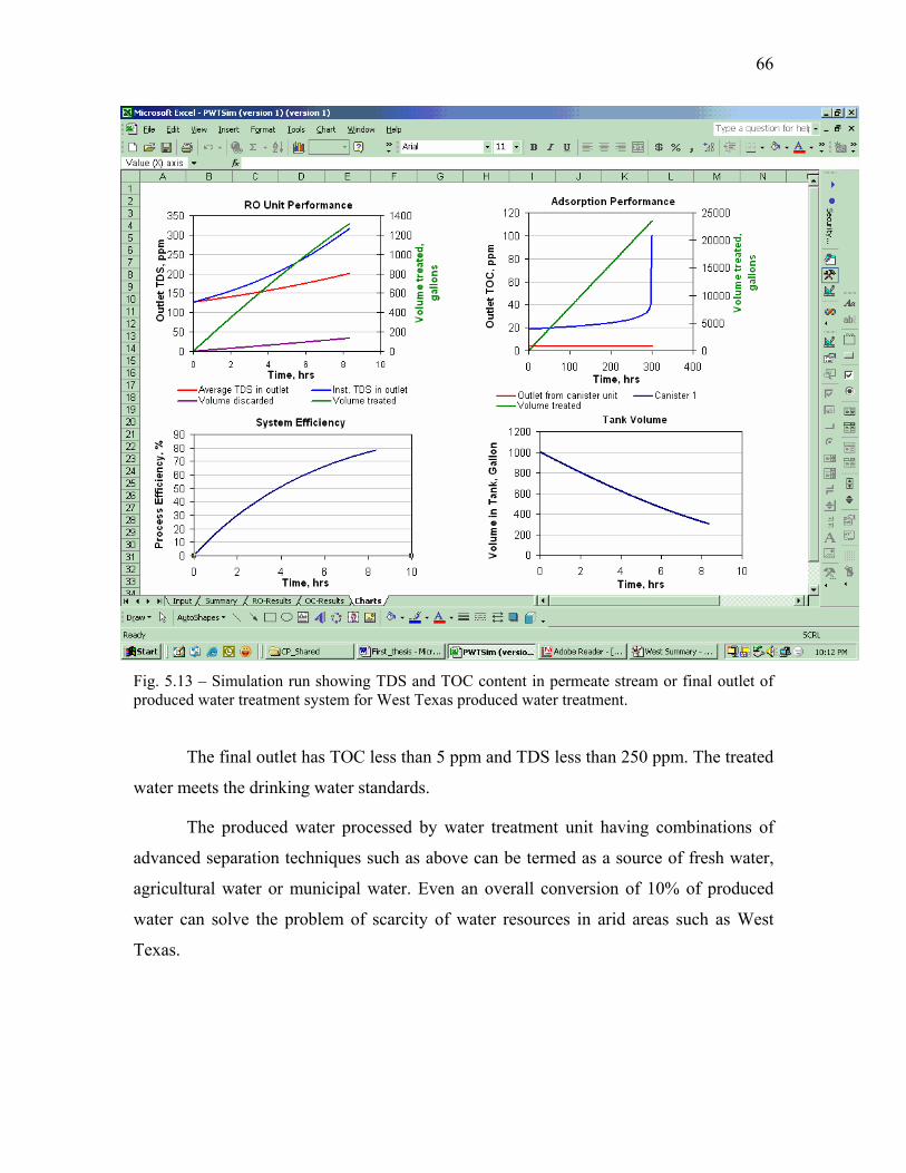
66

Fig. 5.13 – Simulation run showing TDS and TOC content in permeate stream or final outlet of produced water treatment system for West Texas produced water treatment. The final outlet has TOC less than 5 ppm and TDS less than 250 ppm. The treated

water meets the drinking water standards.

The produced water processed by water treatment unit having combinations of

advanced separation techniques such as above can be termed as a source of fresh water,

agricultural water or municipal water. Even an overall conversion of 10% of produced

water can solve the problem of scarcity of water resources in arid areas such as West

Texas.

67

CHAPTER VI

CONCLUSIONS AND RECOMMENDATIONS

6.1 Conclusions

A new approach to manage excessive amounts of produced water is discussed

which can convert produced water as a source of fresh water. We modeled and simulated

the performances of advance separation techniques which can be used to remove oil,

dissolved solids and other hazardous materials from produced water. Two case studies

are discussed, one with lower feed TDS and other with higher feed TDS content to

demonstrate the feasibility of the option of produced water treatment to manage resources

effectively. Following conclusions can be drawn from this study,

1. The conversion of produced water into a source of fresh water is feasible for field

scale application.

2. Organoclay PS12385 can remove more than 90% TOC content of produced water,

provided the series/parallel operation.

3. RO is the best technology available to remove TDS from produced water. It can

remove more than 95% TDS content of produced water.

4. A combination of continuous adsorption and batch RO units is an effective system

for the treatment of produced water and it provides maximum treatment

efficiency.

5. Produced water treatment simulator developed in this study based on empirical

models can simulate produced water treatment process for produced water having

TOC content ranging from 20 – 8000 ppm and TDS content ranging from 500 –

40000 ppm.

6.2 Recommendations

The following recommendations can be made on the basis of the results and

conclusions.

68

1. Detailed experimentation of organoclay adsorption with produced water as feed is

required to study adsorption kinetics and overall performance of fixed bed

adsorption.

2. More RO membranes should be tested to evaluate application of RO operation for

removal of TDS from produced water.

3. Separation techniques other than adsorption and RO should be evaluated to

determine the cheapest and the most efficient of them for produced water

treatment.

4. The research work is required to determine options for handling concentrated

streams from the treatment unit discussed above that can have higher TDS

content, e.g. concentrate to be discarded at the end of each RO batch.

69

NOMENCLATURE

Roman

A = adsorption isotherm parameter

Acs = cross sectional area of packed bed, cm2 or inch2 or ft2

b = hyperbolic parameters depend on operating conditions

B = adsorption isotherm parameter

c = solute concentration in liquid phase that is contacted to adsorbent, ppm

c1 = intercept of straight line, gm oil/gm adsorbent

Cin = TOC content of inlet fluid stream to the adsorption column, ppm

Cp = permeate recovery, %

Cperm = salt concentration in permeate, ppm

Ctds = average salt concentration in feed, ppm

C(t) = TOC content of adsorption column outlet at any time during operation, ppm

D = hyperbolic parameters depend on operating conditions

E = process efficiency or percentage of recovery, %

HTV = initial volume of water in holding tank, gallons

k = adsorption rate constant, min-1 or hr-1

Kads = slope of straight line

L = total length of adsorption column packed with organoclay, cm or inch or ft

mads = co-efficient of adsorption, gm of oil adsorbed/gm of oil inflow

mb = loading capacity, gm oil/gm adsorbent

nk = kinetic order

Pi = pressure at the feed inlet side, psi

Po = pressure at the concentrate outlet side, psi

Pp = pressure at the permeate outlet side, psi

70

Q = volumetric flow rate through the packed bed, GPM or ml/min

*q = equilibrium solute concentration in adsorbent, gm of oil/gm of adsorbent

qoc = throughput of adsorption canister unit, GPM

Rads = adsorption rate, [unit of k] [ppm] kn

Rj = salt rejection, %RT = residence time, min or hr

tb = operation time for RO unit per batch, hrs

ts = stoichiometric time, min or hr

Wpacked = weight of column packed with organoclay, gm or lbs

Woc = weight of packed organoclay, gm or lbs

Wc = weight of unpacked column, gm or lbs

Wads = amount of oil cumulatively adsorbed in packed bed, gm or lbs

Win = amount of oil cumulatively get into the packed bed, gm or lbs

Wout = oil out from the adsorption column, gm or lbs

Greek

ε = porosity of the packed bed

θ = empty bed contact time, min or hr

ρb = bulk density of packed bed, gm of adsorbent/volume of packed bed

71

REFERENCES

1. Dan, D.C.: “ Produced Water Regulations in United States: Then, Now and in the

Future,” paper SPE 77839 presented at the 2002 SPE Annual Technical

Conference, San Antonio, TX, September 29-October 02.

2. Evans, P. and Robinson, K.: “Produced Water Management-Reservoir and

Facilities Engineering Aspects,” paper SPE 53254 presented at the 1999 SPE

Middle East Oil Show, Bahrain, 20-23 February.

3. Mackay, E.J., Collins, I.R., Jordan, M.M., and FEASEY, N.: “PWRI: Scale

Formation Risk Assessment and Management,” paper SPE 80385 presented at the

2003 SPE International Symposium on Oilfield Scale, Aberdeen, UK, 29-30

January.

4. Jun Wan, X., Liu, B., Bai Y., and Liang, S.: “Reinjection of Finely Disposed

Produced-water Reduces Formation Damage in Low Permeability Zones,” paper

SPE 82234 presented at the 2003 SPE European Formation Damage Conference,

The Hague, 13-14 May.

5. Alonzo, Wm. L., Miller, J. A., Miller, D.L., and Hayes, T.D.: “Regional

Assessment of Produced Water Treatment and Disposal Practices and Research

Needs,” paper SPE 029729 presented at the 1995 SPE/EPA Exploration &

Production Environmental Conference, Houston, 27-29 March.

6. Hughes, S.W., Sehsauvafu, S.A., and Slater, J.M.: “Produced Water Treatment

Technologies: A Case Study,” paper SPE 27131 presented at the 1994 Second

International Conference of Health, Safety & Environment in Oil & Gas

Exploration & Production, Jakarta, Indonesia, 25 – 27 January.

72

7. Tao, F.T., Hobbs, R.D., Sides, J.L., Wieser, J.D., Dyke, C.A., Tuohey, D., and

Pilger, P.F.: “Conversion of Oilfield Produced Water Into an Irrigation/Drinking

Quality Water,” paper SPE 26003 presented at the 1993 SPE/EPA Exploration &

Production Environmental Conference, San Antonio, 7-10 March.

8. Tsang, P.B. and Martin, C.J.: “Economic Evaluation of Treating Produced Water

for Potable Use,” paper SPE 86948, SPE International Thermal Operations and

Heavy Oil Symposium and Western Regional Meeting, Bakersfield, 16-18 March,

2004.

9. Hayes T. and Arthur D.: “Overview of Emerging Produced Water Treatment

Technologies,” presented at the 11th International Petroleum Environmental

Conference, Albuquerque, New Mexico (October 2004).

10. Rye, S.E. and Marcussen, E., A: “New Method for Removal of Oil in Produced

Water,” paper SPE 26775 presented at the 1993 Offshore European Conference,

Aberdeen, 7-10 September.

11. Meldrum, N.: “Hydroclones: A solution to Produced-Water Treatment,” paper

SPE 16642 available from SPE, Richardson, Texas (1988).

12. Fernandez, L.G., Soria, C.O., Garcia Tourn, A., and Izquirdo, M.S.: “The Study

of Oil/Water Separation in Emulsion by Membrane Technology,” paper SPE

69554 presented at the 2001 SPE Latin American and Caribbean Petroleum

Engineering, Buenos Aires, 25-28 March.

13. Doyale, D.H. and Brown, A.B.: “Produced Water Treatment and Hydrocarbon

Removal with Organoclay,” paper SPE 63100 presented at the 2000 SPE Annual

Technical Conference, Dallas, Texas, 1-4 October.

73

14. Roberts, J.A.: “Reverse Osmosis System Reduces Demineralised Water Costs,”

paper SPE 27862 presented at the 1994 SPE Western Regional Meeting, Long

Beach, California, 23-25 March.

15. Kasper, D.R.: “Optimization of Reverse Osmosis Treatment of In Situ

Wastewaters,” paper SPE 9492 presented at the SPE 55th Annual Fall Technical

Conference and Exhibition, Dallas, Texas, September 21 – 24 (1980).

16. Siddiqui, M.A.: “Sustainable Development through Beneficial Use of Produced

Water for the Oil and Gas Industry”, M.S. thesis, Texas A&M University-

College Station, TX (December, 2002).

17. Mohamadinejad, H., Knox, J.C., and Smith, J.E.: “Experimental and Numerical

Investigation of Two-Dimensional CO2 Adsorption/Desorption in Packed

Sorption Beds under Non-ideal Flows,” Separation Science and Technology

(2003), 38, Issue 16, 3875-3904.

18. Knaebel, K.S.: “Adsorbent Selection,” Adsorption Research Inc., http

//www.adsorption.com/publications/AdsorbentSel1B.pdf (June 2004).

19. KNAEBELl, K.S.: “A “How To” guide for Adsorber Design,” Adsorption

Research Inc., http://www.adsorption.com/publications/AdsorberDes2.pdf (June

2004).

20. Cooney D. O.: Adsorption Design for Wastewater Treatment, Lewis Publishers,

Boca Raton, Florida (1999) 65–178.

21. Gadre, S.A. and Ritter, J.A.: “New Analytical Solution for Nonlinear Adsorption

and Diffusion in Single Particle,” Chemical Engineering Science (2002), 1197–

1204.

74

22. Yao, C. and Tien, C.: “Approximate Solution of Intraparticle Diffusion Equations

and their Application to Continuous-flow Stirred Tank and Fixed-bed Adsorption

Calculations,” Chemical Engineering Science (1993), 48, 187.

23. Beaton, R.H. and Furnas, C.C.: “Concnetration of Dilute Solutions of Elecrolytes

by Base-Exchange Materials,” Ind. Eng. Chem. (1941), 33, 1500.

24. Hamed, A.M.: “Theoretical and Experimental Study on the Transient Adsorption

Charecteristics of a Vertical Packed Porous Bed,” Renewable Energy (2002), 27,

525 – 541.

25. Cremarsco, M.A., Guirardello, R. and Linda Waing, N.H.: “Adsorption of

Aromatic Amino Acids in a Fixed Bed Column,” Brazilian Journal of Chemical

Engineering (July-Sept 2003), 20, no. 3.

26. Patel, C.V., Barrufet, M.A., and Petriciolet, A.B.: “Effective Resource

Management of Produced Water in Oil and Gas Operations,” presented at the 5th

Canadian International Petroleum Conference (June 2004) ,Calgary, Canada.

75

VITA

Name:

Chirag Patel

Address:

285 Dorset Ct., Piscataway, NJ 08854, US

Education:

Bachelor of Engineering, Chemical Engineering, Nirma Institute of Technology,

Ahmedabad, India, July 01

management of produced water in oil and gas …

Documents