management forecast quality and capital investment decisions

Electronic copy available at: http://ssrn.com/abstract=2298803 Electronic copy available at: http://ssrn.com/abstract=2298803

Management Forecast Quality and Capital Investment Decisions

Theodore H. Goodman Purdue University

[email protected]

Monica Neamtiu The University of Arizona

[email protected]

Nemit Shroff Massachusetts Institute of Technology

[email protected]

Hal D. White University of Michigan [email protected]

June, 2013

Forthcoming at The Accounting Review

ABSTRACT: Corporate investment decisions require managers to forecast expected future cash flows from potential investments. Although these forecasts are a critical component of successful investing, they are not directly observable by external stakeholders. In this study, we investigate whether the quality of managers’ externally reported earnings forecasts can be used to infer the quality of their corporate investment decisions. Relying on the intuition that managers draw on similar skills when generating external earnings forecasts and internal payoff forecasts for their investment decisions, we predict that managers with higher quality external earnings forecasts make better investment decisions. Consistent with our prediction, we find that forecasting quality is positively associated with the quality of both acquisition and capital expenditure decisions. Our evidence suggests that externally observed forecasting quality can be used to infer the quality of capital budgeting decisions within firms. Keywords: management earnings forecasts; voluntary disclosure; capital expenditure;

investment; capital budgeting; managerial ability; forecasting ability. JEL Classification: D83; G31; M41

Data availability: Data are available from public sources identified in the paper.

We appreciate helpful comments from John Harry Evans (senior editor), Amy Hutton (editor), two anonymous referees, Beth Blankespoor, Lian Fen Lee, Roby Lehavy, Greg Miller, Karl Muller, Shyam Sunder, Bill Waller, Joe Weber, and workshop participants at Purdue University, Southern Methodist University, and University of Arizona. Hal White gratefully acknowledges financial support from Ernst and Young.

C O R E M e t a d a t a , c i t a t i o n a n d s i m i l a r p a p e r s a t c o r e . a c . u k

P r o v i d e d b y D S p a c e @ M I T

https://core.ac.uk/display/78053398?utm_source=pdf&utm_medium=banner&utm_campaign=pdf-decoration-v1


1

I. INTRODUCTION

Capital budgeting is one of the most fundamental and important responsibilities of firm

management. A key determinant of successful investment is management’s ability to forecast

project payoffs, because forecasting plays a central role in investment valuation methods (e.g.,

net present value [NPV] calculations, forward-looking price/earnings multiple or other

discounted cash flow analyses). Although these forecasts are a critical component of firm health,

most forecasts are internal and thus not directly observable by external stakeholders. However,

we expect that management’s forecasting ability used to generate internal project payoff

forecasts may transfer to other managerial tasks that involve forecasting, such as providing

external management earnings forecasts. For this specific type of managerial forecast, the

properties are readily observable. Thus, these voluntarily disclosed earnings forecasts may be

valuable to external stakeholders not only because they provide management’s expectations of

next period earnings, but also because they reveal information about managers’ knowledge of the

firm’s economic environment and their ability to forecast future business prospects, a major

component in the investment decision process (Trueman 1986).

This paper investigates whether the quality of voluntarily disclosed management

forecasts can be used to predict the quality of managerial investment decisions. Although prior

research views earnings guidance and capital budgeting as distinct tasks, we argue that both tasks

depend on a common trait—forecasting ability.1 For example, when conducting a corporate

acquisition, managers often begin by making earnings forecasts to assess the intrinsic value of

the potential target (Eccles, Lanes, and Wilson 1999; Cullinan, Le Roux, and Weddigen 2004).

Similarly, managers must predict future project payoffs when selecting among potential capital

expenditure projects (Graham and Harvey 2001). These forecasts require managers to understand

1 In this study, forecasting ability is comprised of management’s ability to: (1) collect high quality information regarding both internal operations (e.g., cost reports, margins, personnel) and the external environment (e.g., competition, industry trends, product demand); and (2) process and synthesize this information, which is a function of experience and innate talent, to develop accurate forecasts. We provide more detail in Section II.


2

the economic environment as well as their competitive position within the environment. This

same understanding is needed when providing earnings guidance as well, because earnings are

essentially the aggregate payoff from past investments. Thus, the quality of managers’ earnings

forecasts is potentially an observable signal of their broader forecasting ability.

Although forecasting future project payoffs is an important part of investment decision-

making, a priori, it is unclear whether we can empirically find a relation between external

management forecasts and managerial investment decisions. First, the quality of a manager’s

external forecasts may not be a good measure of internal forecasting ability, since providing

guidance could encourage managers to engage in earnings management, possibly through

suboptimal investment decisions, so their forecasts appear more accurate (Kasznik 1999;

Roychowdhury 2006). Second, the quality of external forecasts may measure only short-term

earnings forecasting ability. Thus, it may not be associated with the long-term forecasting skills

required for successful capital budgeting.

To test our hypothesis, we examine the relation between management forecasting quality

and the quality of subsequent investments using both investments in other companies (corporate

acquisitions) and investments in fixed assets (capital expenditures).2 We begin by examining the

relation between management forecasting quality and the quality of subsequent acquisition

decisions. We proxy for the quality of acquisition decisions using (i) the stock price reaction to

acquisition announcements (Jensen and Ruback 1983; Masulis, Wang, and Xie 2007; Francis and

Martin 2010), (ii) post-acquisition changes in operating performance (Healy, Palepu, and Ruback

1992), (iii) the probability and magnitude of post-acquisition goodwill write-downs (Gu and Lev

2 We examine both types of investments because they offer unique advantages that complement each other. We examine acquisitions because they are large, high profile corporate events, with publicly available information, such as the exact investment date and specific investment characteristics that we can use in our analyses to provide more robust evidence. In contrast, much less information is publicly available about capital expenditure projects. However, as compared to acquisitions, capital expenditures are less complex investment transactions that do not involve external parties such as investment bankers. As such, forecasting ability and investment valuation may be more directly attributable to managers in a capital expenditure setting. We discuss the role of forecasting ability in both types of investment in Section II.

3

2011), and (iv) the probability of a post-acquisition divestiture (Francis and Martin 2010).

Acquisition announcement returns serve as an ex ante measure of the quality of the acquisition

decision and the remaining three measures serve as ex post measures of acquisition performance.

We use the pre-acquisition three-year average accuracy of managers’ external earnings forecasts

as our measure of forecasting quality.

We find that forecasting accuracy is positively associated with acquisition announcement

returns and post-acquisition operating performance, and negatively associated with the

probability and magnitude of post-acquisition goodwill impairments and the probability of post-

acquisition divestitures. These results suggest that firms providing high quality management

forecasts make better acquisition decisions. Our inferences are robust to controlling for a number

of alternative explanations related to (i) uncertainty in the overall economic environment driving

both forecasting accuracy and investment quality, (ii) agency problems that lead to opaque

disclosures and inefficient investment, (iii) higher financial statement quality and disclosure

quality reducing financing constraints, and thus increasing investment efficiency, and (iv) self-

selection associated with managers voluntarily providing earnings forecasts.

Next, we examine whether the relation between management forecasting accuracy and

acquisition quality is weaker in settings where managerial forecasting ability may not fully

extend to the valuation of other firms. Specifically, we argue that managers’ forecasting ability

extends more easily to firms operating in the same industry and firms with similar earnings

generating processes. Since investment appraisal involves management’s ability to acquire and

process information about industry- and economy-wide prospects, managers can use, or transfer,

this knowledge to more effectively aid the valuation of (i) firms in the acquirer’s industry, and

(ii) firms that have similar earnings generating processes. Consistent with this argument, we find

that management forecast quality is more strongly associated with acquisition announcement

4

returns when the target operates in the same industry and when the target has a similar earnings

generating process, as measured by comovement is prior stock returns.

To provide further support for our prediction and corroborate the evidence documented

using acquisitions, we examine the association between forecasting accuracy and investment

efficiency using capital expenditures as a measure of investment. Investment inefficiency is

defined as investment that differs from the amount that would be predicted given the firm’s

investment opportunities (Brennan 2003). Following a long list of prior studies, we measure

investment efficiency as the magnitude of the deviation of actual investment from the expected level

of investment given the firm’s investment opportunities.3 Consistent with our prediction, we find that

firms providing more accurate forecasts invest more efficiently in capital expenditures.

Our findings contribute to prior research along several dimensions. First, our study

extends the capital investment and the management forecast literatures by considering the critical

role played by managerial forecasting ability in both short-term earnings forecasting and long-

term capital investment decisions. Typically, the management forecast and investment literatures

operate as distinct strands of research. Most of the prior capital investment literature focuses on

the value created or destroyed by corporate capital investment and on whether firms’ level of

capital investment falls in line with their investment opportunity set (Hubbard 1998; Stein 2003),

whereas much of the prior management forecast research examines the determinants of

management forecasting behavior and its consequences for capital markets (Hirst, Koonce, and

Venkataraman 2008). These two research streams offer little discussion on whether the abilities

related to capital budgeting or generating earnings forecasts extend to other managerial tasks. By

highlighting the relation between managerial tasks that draw on common forecasting ability, our

3 See e.g., Fazzari et al. (1988), Wurgler (2000), Biddle and Hilary (2006), Richardson (2006), Whited (2006), Acharya, Almeida, and Campello (2007), McNichols and Stubben (2008), and Biddle, Hilary, and Verdi (2009).

5

research identifies an observable proxy for the quality of internal project payoff forecasting. Our

findings also suggest that, when studying the determinants and consequences of managers’

earnings guidance, researchers should regard the quality of earnings forecasts as a broader

measure of forecasting ability and not simply as a means for providing information about

managers’ expectations of next period earnings.

Second, our findings may be relevant to market participants and regulators, as they

inform the recent debate regarding the cessation of management earnings forecasts. Corporate

professionals (Business Roundtable Institute for Corporate Ethics and CFA Institute Centre for

Financial Market Integrity 2006) and some academics (Fuller and Jensen 2002) argue that

managers should end the practice of providing quarterly earnings guidance because it induces

myopic behavior by managers. However, proponents contend that guidance can better align

external stakeholder expectations with those of management, thereby reducing information

asymmetry. We provide empirical evidence suggesting that the quality of these forecasts can be

used as a valuable measure of broader managerial forecasting ability related to investment. Thus,

our findings point to an additional benefit of voluntarily disclosed forecasts that should be

considered in the guidance cessation debate.4

Third, our research provides greater insight into the nature of managerial ability.

Trueman (1986) analytically shows that managers may be motivated to release earnings forecasts

because it gives investors a more favorable assessment of the manager's ability to anticipate

changes in the economic environment and to adjust investment decisions accordingly. However,

there is little empirical evidence in the prior literature about whether managerial ability can be

inferred from their earnings forecasts. We add to this literature by providing evidence consistent

4 Note that our findings do not imply that issuing guidance is optimal, or even encouraged, for all firms. Our findings only suggest that external stakeholders of firms that provide guidance may be able to draw inferences about management’s investing ability relative to that of managers of other firms that also provide earnings guidance.

6

with the notion that the quality of external management forecasts can serve as a measure of a

broader forecasting ability related to investment decision inputs.5

Finally, our paper contributes to the nascent literature that explores the relation between

external disclosures and internal decision-making. For example, Hemmer and Labro (2008)

provide analytical evidence that the properties of the financial reporting system affect the quality

of the managerial accounting system, and thus the quality of corporate investment decisions.

Similarly, Durnev and Mangen (2009), McNichols and Stubben (2008), Biddle et al. (2009),

Bens, Goodman, and Neamtiu (2012), Badertscher, Shroff, and White (2013), Shroff, Verdi, and

Yu (2013) and Shroff (2013) provide arguments and evidence linking external reporting to

internal investment decisions. However, none of these studies examine the relation between

managers’ voluntary disclosure quality and the quality of their internal investment decisions.

Section II next discusses the motivation for the study. Section III describes the research

design, descriptives, and results. Section IV discusses robustness tests, and Section V concludes.

II. MOTIVATION

In this section, we discuss the central role forecasting plays in the assessment of potential

corporate investment projects. We also discuss why the quality of external managerial earnings

forecasts may serve as a useful signal of managers’ internal forecasting ability.

Forecasting and Corporate Acquisitions

Corporate acquisitions typically require a large expenditure by the acquiring firm and a

rigorous and thorough due diligence process. This process requires a deep understanding of: (i)

the target value as a stand-alone business when operated by its current management; (ii) the

5 Note that there are many drivers of managerial ability related to leadership, communication, delegation, business acumen, etc. We focus on one particular aspect of managerial ability, i.e., forecasting ability, because it is directly related to both investment decisions and earnings forecasts.

7

value of potential synergies; and (iii) the maximum bid price the acquirer should pay. We expect

each of these steps to be dependent on the manager’s earnings forecasting ability.6

First, earnings forecasting ability plays a central role in valuing the target company.

Practitioner resources (Eccles, Lanes, and Wilson 1999; Cullinan, Le Roux, and Weddigen 2004)

and M&A textbooks (Copeland, Koller, and Murrin 2000) suggest that managers begin the

acquisition valuation process by calculating the target’s stand-alone value. Copeland et al. (2000)

indicate that the independent valuation of the target on a stand-alone basis should be the essential

underpinning of any deal. Common valuation approaches include using a forward-looking

price/earnings (P/E) multiple or a discounted cash flow (DCF) analysis, both of which rely

heavily on earnings forecasts as inputs for the valuation (Chaplinsky, Schill, and Doherty 2006).7

Second, once acquirers determine the stand-alone value of a target, they must determine

the value of any synergies. Here again, managers must rely on their forecasting ability to

estimate the synergies involved in an acquisition, which requires knowledge of the acquiring and

target firms’ cost structures and revenue drivers. For example, a common type of synergy is cost

savings from eliminating facilities and expenses that are no longer necessary when the two

businesses are consolidated. Revenue enhancement synergies are also possible if the acquirer and

the target achieve higher sales growth together than the firms could do operating on their own.

Successfully forecasting these synergies requires a clear understanding of the firms’ economic

environments and cost and revenue structures. Such an understanding is also central to

successfully forecasting earnings.

6 For ease of exposition, we discuss the role of forecasting in three distinct steps. However, separating these steps, conceptually or empirically, is very difficult because they are unlikely to be independent. 7 Successful capital budgeting decisions are those that generate cash receipts in excess of disbursements. Thus, it is reasonable to expect that managers forecast future cash flows to evaluate potential projects. However, over finite intervals, cash flows are not necessarily as informative as earnings because cash flows have timing and matching problems that cause them to be a ‘noisy’ measure of project performance. The purpose of earnings is to smooth transitory fluctuations in cash flows to better measure firm/project performance over finite intervals (Dechow 1994). Over the life of a project/firm, aggregate cash flows by definition equal aggregate earnings. For the purpose of our paper, we use both cash flows and earnings interchangeably to mean project payoffs.

8

Lastly, acquirers need to determine their maximum bid price. This price is a direct

function of the target’s stand-alone value and the value of the potential synergies, making it

dependent on forecasting ability as well. The extent to which the final offer price is close to the

acquirer’s maximum bid price depends on how the allocation of gains from the business

combination is negotiated between the acquirer and target (Grossman and Hart 1980).8 This

negotiation process also depends on forecasting ability, making negotiating ability and

forecasting ability complements, as effective negotiations are not possible unless the acquirer has

clear insight into the value of the target.

We note, however, that the acquisition process typically involves parties other than the

acquirer and target. In particular, investment bankers frequently aid the acquirer in valuing the

target firm and provide assistance in negotiating the deal price and other terms. Servaes and

Zenner (1996) find that acquirers retain investment bank advisors when the deals are more

complex and when the acquirer lacks prior acquisition experience. Although investment banks

often play an advisory role in important phases of the acquisition, the ultimate responsibility for

the acquisition valuation process and the final investment decision rests with the acquirer’s

management. This view is supported by prior research (Lehn and Zhao 2006), which shows that

the acquirer’s manager experiences elevated turnover probabilities following poor acquisitions.

Forecasting and Capital Expenditures

Capital expenditures, which typically require fewer resources than business acquisitions,

are another common type of investment in real assets. We again expect forecasting ability to play

a central role in capital expenditure decisions because the ability to better forecast each potential

project’s future payoffs provides management with a more precise estimate of the project’s net

present value. In fact, the same forecasting factors, such as a series of projected future payoffs, a

8 Exactly how much of the total estimated transaction value is transferred to the target depends in part on the relative bargaining power of the target and acquirer. If there is intense competition among multiple bidders for a target, the acquirer is likely to have less negotiating power (Jensen and Ruback 1983).

9

terminal value, etc., and valuation methods, such as DCF, are again applicable when valuing

capital expenditures (Brennan 2003; Chaplinsky et al. 2006).

There are, however, some differences with respect to forecasting between the acquisition

and capital expenditure settings. For example, because capital expenditures typically reflect

purchases of long-term assets that are related to existing operations, a manager’s ability to

forecast her own firm’s earnings is likely to extend to forecasting the payoffs of the new assets.

In contrast, acquisitions may involve targets in other industries or with different earnings

generating processes, where a manager’s forecasting ability might not extend as readily. Capital

expenditure decisions are also less likely to involve third parties, such as investment bankers,

making the forecasting and valuation process more directly attributable to managers.9 Because of

these differences, it is important to examine both acquisitions and capital expenditures to glean a

more complete understanding of the role of managerial forecasting ability with respect to the

quality of investment decision making.

External Earnings Forecasts as a Proxy for Managerial Forecasting Quality

Earnings represent a summary measure of the payoffs from past investments and are

precisely what managers are interested in estimating when choosing among alternative

investment projects (Graham, Harvey, and Rajgopal 2005). Thus, managers likely draw on

similar information and skills when generating external earnings forecasts and internal project

payoff forecasts. If external earnings forecasts serve as a useful signal of managers’ forecasting

ability with respect to the future returns from investments, we expect the quality of external

forecasts to be associated with subsequent investment quality. Consistent with our argument,

Trueman (1986) analytically demonstrates conditions under which management forecasts allow

9 Unfortunately, because individual capital expenditures are often of smaller magnitude than corporate acquisitions, there is less detail on the nature of the capital expenditure relative to acquisitions. This lack of detail makes it difficult to explore cross-sectional variation based on the types of the expenditures or to link expenditure decisions to subsequent outcomes, such as divestitures and impairments.

10

investors to better assess a manager’s ability to anticipate changes in the economic environment

and adjust production plans accordingly.

Managers’ forecasting ability is driven by two important factors: (i) the availability of

high quality information regarding internal operations and the external environment, and (ii)

their ability to process this information in developing forecasts. Supporting the argument that the

ability to process information is important, Simon (1973, 270) argues that “…the scarce resource

is not information; it is processing capacity to attend to information. Attention is the chief

bottleneck…and the bottleneck becomes narrower…as we move to the tops of organizations…”

Supporting the role of information systems in generating high quality forecasts, Feng, Li, and

McVay (2009) find that managers of firms with material weaknesses in their internal control

over financial reporting provide less accurate earnings forecasts.

While we cannot disentangle the individual effects of information system quality and

managerial forecasting ability, we note that information systems are designed and implemented

by managers to aid them in making better operating decisions. Therefore, the quality of internal

systems can be at least partly attributed to managerial ability. For example, Bamber, Jiang, and

Wang (2010) suggest that managers who have earned an MBA degree, and thus have formally

learned how to collect and process relevant information for forecasting, provide higher quality

forecasts. Accordingly, we assume that the accuracy of management forecasts arises from both

managers’ ability to obtain high quality information, by putting in place appropriate information

systems, and their skill in processing and incorporating this information into their forecasts.

Ex-ante, it is an open question whether external earnings forecasts can serve as a signal of

managers’ internal forecasting ability with respect to investment for two reasons. First, the public

dissemination of earnings forecasts may provide incentives for managers to engage in financial

reporting manipulations or suboptimal investments to meet their own earnings targets (Fuller and

Jensen 2002; Roychowdhury 2006; Cohen, Mashruwala, and Zach 2010), which would confound

11

the forecasting ability signal.10 For example, a manager may appear to have high quality external

forecasts, but in reality the manager may have engaged in earnings management and actually has

lower forecasting ability (Kasznik 1999). Alternatively, managers may have strong internal

forecasting abilities, but strategically bias external forecasts to meet an objective other than

forecasting accuracy, such as walking down analysts’ earnings expectations, misleading

competitors, and manipulating their stock price for insider trading and/or compensation reasons

(Cotter et al. 2006; Matsumoto 2002; Aboody and Kasznik 2000). Thus, the quality of the

external forecasts may not capture the manager’s actual forecasting ability. On the other hand,

both the ‘settling up’ of external forecasts and their recurring nature impose disciplinary and

potential legal constraints on managers’ freedom to bias their expectations from their internal

projections (Baginski, Hassell, and Kimbrough 2002). As such, it is unclear to what extent

managers make substantive forecast adjustments from their actual expectations.

Second, there are differences in the forecasting horizon between forecasting earnings and

forecasting investment payoffs. It is possible that the quality of external forecasts measures only

short-term earnings forecasting ability, whereas the successful implementation of commonly

used investment valuation methods, such as a DCF analysis, requires not only short-term, but

also long-term earnings forecasting ability and terminal value estimates. Although these two

forecasting tasks are distinct, we expect the quality of the two tasks to be positively related in

that they rely on the manager’s ability to assess the external economic environment, their firm’s

place in that environment, potential future changes in competition, demand, technology,

production costs, etc., as well as the quality of the firm’s internal information systems. We

10 The above evidence also suggests that the act of providing management forecasts may lead to suboptimal investment decisions. For example, Cheng, Subramanyam and Zhang (2007) document that dedicated guiders engage in myopic R&D investment behavior relative to occasional guiders, which results in adverse effects on long-term growth. Moreover, Graham, Harvey and Rajgopal (2005) find that managers pass up positive NPV projects to meet their earnings targets. Therefore, ceteris paribus, it is plausible that firm that issue earnings forecasts invest less efficiently than firms that do not forecast earnings. However, our interest lies in documenting variation in investment efficiency conditional on managers issuing earnings forecasts.

12

expect that short-term forecasting ability is a necessary, but not sufficient, condition for long-

term forecasting ability. In other words, on average, we expect that managers who are unable to

accurately forecast earnings in the short-term will also forecast poorly over longer horizons.

III. RESEARCH DESIGN AND EMPIRICAL RESULTS

Managerial Forecast Quality Measure

We use the quality of earnings forecasts to proxy for managerial forecast quality because

earnings represent the aggregate payoffs from past investment decisions and because most other

managerial forecasts are internal and not observable by outsiders. To assess the quality of

management earnings forecasts, we focus on forecast accuracy following prior literature (Baik et

al. 2011; Bamber et al. 2010; Feng et al. 2009; Hirst et al. 2008). Our intuition is that a manager

who has a better understanding of the overall economic environment and her firm’s place in that

environment should forecast more accurately and thus engage in better investment decisions. We

use the absolute magnitude of forecast errors to measure forecast accuracy.11

We collect information about management earnings forecasts and actual earnings per

share (EPS) from First Call’s Company Issued Guidance (CIG) and the First Call’s Actuals

databases. For each forecast, accuracy is measured as the absolute value of the difference

between the management EPS forecast and the actual EPS, divided by the stock price. For range

forecasts, we use the mid-point of the range following prior literature (e.g., Rogers and Stocken

2005).12 We also follow prior literature (Rogers and Stocken 2005) and use annual, rather than

11 For example, suppose that both firm A and firm B have actual earnings of $1.00. If firm A’s manager forecasts $1.01 and firm B’s manager forecasts $0.85, we argue that manager A (who is able to forecast closer to the actual realization) has better forecasting ability than manager B, even though manager A was optimistically biased in her forecast. Similarly, if manager A (B) forecasted $0.99 ($1.15), we would argue that manager A has better forecasting ability, even though she was conservatively biased in her forecast. That is, the sign of the forecast error is less relevant with respect to the manager’s ability to predict the actual earnings number. Further, we note that biases in forecasts may be correlated with agency problems that lead to inefficiency investment decisions. We address the role of agency problems in affecting investment efficiency in Section IV. 12 Following prior research (e.g., Rogers and Stocken 2005), we remove open-ended forecasts because it is difficult to measure forecasting accuracy when we cannot unambiguously compare the forecast to the realized earnings.

13

quarterly, forecasts because they relate to earnings that are audited, and thus are less amenable to

manipulation. To ensure that we do not include earnings pre-announcements and that we allow

some time between the forecast announcements and earnings realizations, we require forecasts to

be issued at least three weeks before the earnings announcement date.

We calculate our forecast accuracy measure, Forecasting Accuracy, as the average

accuracy for all annual forecasts issued in the three-year period before the investment decision

(see Figure 1). We then multiply this average by negative one to transform it into an increasing-

in-quality measure. The long measurement window helps mitigate short-term effects that may

bias forecast quality, including earnings management or short periods of forecasting ‘luck,’ both

of which are unlikely to be sustainable (Hilary and Hsu 2011).

The Relation between Forecasting Accuracy and Corporate Acquisition Quality

In this section, we examine the relation between management forecasting quality and

acquisition quality. We measure acquisition quality using an ex ante estimate of acquisition

quality (i.e., acquisition announcement returns) as well as three ex post estimates of acquisition

quality (i.e., post-acquisition change in operating performance, post-acquisition probability and

magnitude of goodwill impairments, and post-acquisition probability of divestitures).

Corporate Acquisition Announcement Return Analysis

Following a large body of prior research (e.g., Asquith, Bruner, and Mullins 1983; Jensen

and Ruback 1983; Lehn and Zhao 2006; Masulis et al. 2007; Francis and Martin 2010), we use

the stock return around the acquisition announcement to proxy for the quality of the investment

decision. This approach assumes that the market incorporates information in stock prices

efficiently, so that the announcement return is an unbiased estimate of the impact of an

acquisition on the wealth of acquiring-firm shareholders (Moeller, Schlingemann, and Stulz

2004). Since almost all acquisitions of public companies are publicly announced in a salient

14

manner, the short window return is likely to capture the market’s assessment of the acquisition

decision and is relatively less subject to misspecification than other measures of acquisition

quality, such as long-window return measures (Shleifer and Vishny 1997).

We collect our acquisition sample from the Securities Data Corporation’s (SDC) US

Mergers and Acquisitions database. We identify acquisitions announced between January 1,

1996 and December 31, 2008 that meet several criteria: (i) the acquirer is a US public company;

(ii) the acquirer has annual financial statement information available from Compustat and stock

return data from the CRSP Daily Stock Price and Returns file; (iii) the acquisition is completed.

We retain only acquisitions that are at least five years apart for each firm. For firms engaging in

multiple acquisitions within a five-year period, we retain only the first acquisition in this period.

We impose this condition because prior literature finds strong evidence that (i) repeat acquirers

have lower acquisition announcement returns for their later acquisitions than they do for their

earlier acquisitions (Fuller, Netter, and Stegemoller 2002; Conn, Cosh, Guest, and Hugues 2004;

Ahern 2008; Ismail 2008) and (ii) management forecast accuracy is fairly stable overtime

(Hutton and Stocken 2009).13 Therefore, when collectively viewed, these results suggest that we

should not necessarily expect a relation between management forecast accuracy and the

announcement returns for subsequent acquisitions undertaken in a series.14

13 Importantly, we also note that the reasons why repeat acquirers have lower announcement returns for later acquisitions are unlikely to be related to forecasting accuracy. Specifically, prior research identifies three potential reasons why repeat acquirers have declining announcement returns: (1) the opportunity set hypothesis, which predicts that the best targets are acquired first and worse targets later (Klasa and Stegemoller 2007); (2) the hubris hypothesis, which predicts that early success leads to managerial overconfidence and thus overbidding in later deals (Aktas, de Bodt, and Roll 2009); and (3) the agency hypothesis, which predicts that management interests become less aligned with shareholder interests as a firm matures. Thus, later deals may be made to generate private managerial benefits, not shareholder wealth gains (Moeller, Schlingemann, and Stulz 2004). Since it is a significant empirical challenge to fully control for all the reasons why we might observe lower announcement returns for later acquisitions by serial acquirers, the declining pattern observed in acquisition announcement returns contaminates the interpretation of forecast accuracy when we include all acquisition in our sample. 14 In untabulated analyses, we find that our acquisition announcement test results are not robust to using the sample of all acquisitions. While we believe this result is to be expected given the patterns described above, we caution readers that our inferences do not hold for the sample of all acquisition announcements.

15

To test our prediction regarding the association between forecast quality and the quality

of subsequent acquisitions, we use the following regression model:

CAR t = γ0 + γ1Forecasting Accuracy [t-3, t-1] + γi CONTROLS + et, (1)

where CAR is the three-day cumulative abnormal return around the acquisition announcement

and abnormal returns are measured using (i) the market model or (ii) the market-adjusted return,

where Table 1 provides a detailed description of the variable construction approach.15

Forecasting Accuracy is defined above, and we predict γ1 > 0. We cluster standard errors by

four-digit SIC industry and fiscal period end to allow for residual correlation within an industry

and fiscal period. Our regression model also includes industry and time fixed effects.

CONTROLS is a vector of control variables measuring acquirer and acquisition

characteristics as well as the overall uncertainty in the firm’s environment. With respect to

acquirer characteristics that are likely to affect acquisition announcement returns, following prior

research we control for Firm Size using the natural log of total assets, Tobin’s Q, the return on

assets (ROA), sales growth (Growth), Leverage, and Stock Return. We measure all firm

characteristics as of the last fiscal year end preceding the acquisition announcement. Tobin’s Q,

ROA, Growth and Firm Size are associated with a firm’s growth opportunities and the

availability of financing (Moeller et al. 2004; Dong et al. 2006). Leverage captures monitoring

by creditors that may limit a firm’s ability to overinvest (e.g., Maloney et al. 1993; Masulis et al.

2007). Finally, we control for the acquirer’s pre-acquisition Stock Returns because prior work

(e.g., Rosen 2006) documents that an acquirer’s twelve-month stock return trailing the

announcement date is a determinant of the acquisition announcement return. In addition, the

management forecast literature finds that earnings forecast properties are a function of firm size

(e.g., Ajinkya, Bhojraj, and Sengupta 2005), growth opportunities (e.g., Feng et al. 2009),

15 In untabulated analyses, we re-estimate our acquisition announcement test using the average daily abnormal return between the announcement date and the completion date, and Forecasting Accuracy is still positive and significant at the 1% level.

16

leverage (e.g., Hutton, Lee, and Shu 2012) and past stock returns (e.g., Gong, Li, and Wang

2011). We include these controls to mitigate the concern of correlated omitted variables. The

definitions of all our control variables are detailed in Table 1.

In addition, we control for overall economic uncertainty to mitigate concerns that firms

operating in environments with less uncertainty find it easier to forecast future earnings and

expected future payoffs from their investment opportunities. That is, in a more certain

environment, it is easier to both (i) forecast earnings and (ii) filter out poor investment decisions.

In contrast, where there is more uncertainty, forecast errors will naturally be larger and firms will

tend to make poorer investment decisions. Thus, instead of managers’ forecasting ability

affecting both external forecast quality and the quality of their investment decisions, it could be

general uncertainty that affects both.

To mitigate the uncertainty concern, we control for Analyst Forecast Accuracy and

Analyst Forecast Dispersion over the same period that we measure management forecast

accuracy (Zhang 2006; Hutton and Stocken 2009).16 We also control for earnings and stock

return volatility (Stdev. ROA; Stdev. Stock Returns) as well as Earnings Persistence (Hutton and

Stocken 2009) to mitigate any potential residual effect of uncertainty on management forecast

accuracy and investment quality. Finally, to the extent managers who operate in a more uncertain

business environment are likely to issue a less precise forecast (i.e., issue wider range forecasts),

we include a measure of Forecast Precision, calculated as the average precision of all forecasts

issued in the three-year period prior to the investment decision.

Next, we control for Forecast Horizon, measured as the natural log of the number days

between the forecast announcement date and fiscal period end date. We use the average horizon

16 Hutton and Stocken (2009) use a relative accuracy measure computed as the manager’s forecast accuracy less the consensus analyst forecast accuracy. We decompose this measure and include each accuracy measure separately in the regression to allow the coefficients to vary. However, in untabulated analyses we find that our inferences are robust to using the relative accuracy measure.

17

of all forecasts issued in the three-year period before the investment decision. Forecast Horizon

can play an important role in shaping accuracy, potentially influencing our inferences about

managers’ forecasting ability drawn from observed accuracy. For example, an accurate forecast

issued a year before the fiscal period end date signals a greater level of forecasting ability than an

equally accurate forecast issued a month before the period end date. Consistent with this

intuition, prior studies, such as Ajinkya et al. (2005) and Hutton et al. (2012), document that

timelines is an important determinant of forecasting accuracy.

Consistent with prior research, we also control for the target’s public status – Public

Target (Chang 1998; Fuller, Netter, and Stegemoller 2002). Private targets have concentrated

ownership, and thus the owners of private targets become large shareholders of the acquirer so

that they have incentives to monitor the management of the acquiring firm (e.g., Chang 1998).

This is especially the case when the acquisition is entirely paid for using the acquirer’s stock. We

control for whether the target is located in the same country as the acquirer, Domestic Target,

following Moeller et al. (2004), and the method of payment, Cash M&A and Stock M&A,

following Travlos (1987) and Moeller et al. (2004). We include Cash M&A in our regression

because it is more likely that cash acquisitions are the result of free cash flow problems, as

proposed by Jensen (1986) (see Shleifer and Vishny 1997). We control for Stock M&A because

arbitrageurs put pressure on the stock price of the acquiring firm for 100% equity offers for

public firms (Mitchell et al. 2004). We also control for Diversifying Acquisitions because prior

research finds that diversifying acquisitions are a sign that managers are trying to build larger

and more stable empires, and thus have lower announcement period returns (Morck, Shleifer,

and Vishny 1990).

We control for the size of the target relative to the acquirer, Relative Target Size, to adjust

for the impact of an acquisition on the equity market capitalization of the acquiring firm. If a

dollar spent on acquisitions has the same positive payoff, irrespective of the size of the

18

acquisition, the abnormal return should increase in the size of the target relative to the size of the

acquirer (Asquith, Bruner, and Mullins 1983). Finally, we control for whether the acquisition

was hostile, Hostile Takeover (Schwert 2000), and the number of bidders competing to acquire

the target, No. of Bidders (Mitchell et al. 2004). We control for No. of Bidders, as competition

among bidders increases the price paid by the acquirer, thereby lowering returns to acquiring-

firm shareholders (Moeller et al. 2004), and we control for Hostile Takeover, as Schwert (2000)

finds that hostile acquisitions have lower abnormal returns than friendly acquisitions.

Table 2 Panel A presents descriptive statistics for the variables in equation (1). The

average acquisition announcement return is close to zero, which is consistent with prior research

(Malmendier and Tate 2008; Bens et al. 2012). The interquartile range for both the Market

Model CAR and the Market Adjusted CAR reveals that there is considerable variation in market

responses (Q1 = -0.022, Q3 = 0.034), which is important, because our analysis examines whether

variation in manager forecasting ability can explain cross-sectional variation in these

announcement returns.17 Panel A also presents descriptive statistics of our main independent

variable, Forecasting Accuracy, and the other management forecast characteristics.

Table 2 Panel B reports the results from estimating equation (1). We find that the

coefficient for Forecasting Accuracy is positive and significant with a t-statistic of 2.03 when

announcement returns are measured using a Market Model CAR, and 1.90 using a Market Adjust

CAR. This suggests that managers who generate more accurate forecasts make better acquisition

decisions than managers who provide less accurate forecasts, which is consistent with our

prediction.18 The coefficients for the control variables are signed consistently with those

17 Untabulated descriptive statistics indicate that no individual year contains more than 10% of our acquisition sample. In addition, there does not appear to be a time trend where the sample size is dramatically increasing or decreasing over time. 18 An alternative explanation for our results is that some managers only provide external forecasts when fairly certain of outcomes and select only new investment projects with a high probability of success. This may lead to a positive association between forecast accuracy and investment quality in the cross-section that is unrelated to forecasting ability. To address this concern, we control for forecast frequency. Specifically, we add forecast

19

documented in prior research. For example, the coefficients for Firm Size and Tobin’s Q are

negative and significant (Moeller et al. 2004), the coefficient for Diversifying Acquisition is also

negative and significant (Morck et al. 1990), and the coefficient for Relative Target Size is

positive and significant (Asquith et al. 1983). Finally, we also find that announcement returns are

more negative for acquisitions of public targets (Chang 1998) and acquisitions completed by

firms operating in uncertain environments, those firms with high Analyst Forecast Dispersion.

Post-Acquisition Change in Operating Performance Analysis

Next, we examine post acquisition accounting data to test for changes in operating

performance following acquisitions. Specifically, we examine post-acquisition changes in the

acquirer’s return on assets and cash flow from operations (Healy et al. 1992). Conceptually, we

focus on both income before extraordinary items and cash flows because they represent the

actual economic benefits generated by the assets. Since the level of economic benefits is affected

by the assets employed, we scale both measures by the assets employed to form a return measure

that can be compared across time and across firms. We examine the average post-acquisition

performance in the three years following the acquisition completion. We employ the regression

model described in equation (1), but change the dependent variable to the average change in the

accounting based measures of performance from three years before the acquisition

announcement to three years after the acquisition completion (see Figure 1, Panel B). Since we

require three years of accounting data both pre- and post-acquisition, our sample size is reduced

by roughly 30% from that used in the acquisition announcement analyses. Table 3, Panel A

presents the descriptive statistics of the variables used in these regressions. We note that our

sample characteristics are very similar to those documented in Table 2, Panel A.

Table 3, Panel B presents the results from these tests. We find that the coefficient for

Forecasting Accuracy is positive and statistically significant when we use the Change in ROA

frequency as a control variable in the regressions presented in Table 2. Forecasting Accuracy remains statistically significant at the 1% in these untabulated tests.

20

and the Change in CFO as the operating performance measure. However, we note that when

Change in ROA is the dependent variable, the coefficient for Forecasting Accuracy is at best

marginally significant using a one-tailed test (one-tailed p-value = 0.058). These results suggest

that firms with higher forecasting accuracy engage in more profitable acquisitions.

Post-Acquisition Goodwill Impairment Analysis

We next examine goodwill impairments as a measure of acquisition quality. Specifically,

following recent studies, such as Doellman and Ryngaert (2010) and Gu and Lev (2011), we

interpret goodwill impairment losses recorded in the post-acquisition period as an indication of a

lower quality investment decision. Since goodwill represents the difference between what the

acquirer pays for the target and the fair value of the target’s separable assets, impairment charges

related to prior acquisitions’ goodwill represent cases where the premium paid above the value of

the separable assets is no longer justified. While monitors, such as auditors, play a role in

requiring firms to record goodwill impairments, managers also have significant discretion in the

application of impairment rules (Ramanna and Watts 2011). However, we expect that a

manager’s discretion would play a larger role in determining the amount of an impairment than

in determining whether an impairment occurs. Accordingly, we examine both the probability and

the magnitude of impairments in the three years following an acquisition.

We expect that acquirers with higher pre-acquisition forecasting accuracy are less likely

to record goodwill impairments in the post-acquisition period. We use the following logistic

(OLS) regression model when the dependent variable is the existence (magnitude) of an

impairment to test our prediction:

Goodwill Impairment t = γ0 + γ1Forecasting Accuracy [t-3, t-1] + γi CONTROLS + et , (2)

where Goodwill Impairment is either (i) an indicator variable that takes a value of one (zero) if a

firm records (does not record) an impairment following the acquisition, or (ii) the magnitude of

the impairment. Forecasting Accuracy and CONTROLS are as defined as earlier. Figure 1, Panel

21

C provides a timeline of our variable measurement windows. Our regressions include year and

industry fixed effects, and we cluster standard errors by industry and year. We estimate equation

(2) using a sample of acquisitions that generate significant goodwill amounts, which we define as

an increase in goodwill greater than or equal to 5% of total assets.19 To increase our sample size,

and thus the test’s power, we retain all acquisitions that generate large goodwill increases, as

opposed to retaining only the first deal in a series, as for the CAR analysis.20, 21

Since our sample differs from that used in the previous analyses, Table 4, Panel A re-

tabulates the descriptive statistics for the goodwill sample. The descriptive statistics indicate that

the characteristics of the firms included in the goodwill impairment test are similar to the

characteristics of firms used in our acquisition announcement analysis. Firm Size, Return on

Assets, Leverage, Growth, etc. have similar values in both tables. More importantly, the forecast

characteristics are also very similar with a median Forecasting Accuracy of -0.013 in Table 2,

Panel A, and -0.010 in Table 4, Panel A.

Table 4, Panel B presents the results from estimating equation (2). We find that the

coefficient for Forecasting Accuracy is negative and statistically significant across both

specifications, consistent with our hypothesis that managers with high forecasting ability make

better investment decisions.22

19 In sensitivity tests, our conclusions do not change when we rerun our analysis using 1% of total assets as a cut-off point for the magnitude of goodwill increases as well as when we use the full sample without any cut-off point. 20 We use Compustat to identify our large goodwill generating acquisitions because this information is not available on SDC. However, a limitation of this approach is that we do not have transaction-specific characteristics for all the deals in this sample. 21 Requiring both that the acquisition be first in the series and that there be at least a 5% increase in goodwill is not feasible. Using both criteria would reduce our sample size substantially because the first acquisitions are not necessarily those that create large goodwill increases. 22 The accounting rules for goodwill impairments changed during our sample period with the implementation of SFAS 142 in 2001. Prior to SFAS 142, firms were required to amortize goodwill, and sufficiently high amortization could have reduced or eliminated goodwill impairments in the pre SFAS 142 period. In addition, SFAS 142 increased the regularity of impairment testing. Taken together, these changes may increase the probability that, in the post SFAS 142 period, a firm whose goodwill is overvalued will record an impairment loss. Accordingly, we re-estimate our goodwill impairment model using only observations after 2002, and our results do not change. Specifically, we continue to find that the coefficient for Forecasting Accuracy is negative and statistically significant at the 5% level.

22

Post-Acquisition Divestitures Analysis

Prior studies, including Mitchell and Lehn (1990) and Francis and Martin (2010), suggest

that post-acquisition divestitures indicate poorer acquisition decisions. The authors interpret the

divestiture decision as evidence that acquisition strategies failed to increase and perhaps,

decreased value. Therefore, we also measure the ex-post success of an acquisition by observing

the likelihood of a subsequent divestiture. Our analysis of divestitures complements the goodwill

impairment tests, because some firms will divest a poor acquisition rather than continue the

operations of the acquired unit and incur an impairment charge. Assuming that post-acquisition

divestitures are indicative of poor acquisition decisions, we expect that firms with greater pre-

acquisition forecasting quality are less likely to have a subsequent divestiture. We test this

prediction using the following logistic regression model:

Divestiture t = γ0 + γ1Forecasting Accuracy [t-3, t-1] + γi CONTROLS + et, (3)

where Divestiture is an indicator variable that takes a value of one (zero) if an acquisition results

in (does not result in) a subsequent divestiture.23 An acquisition is defined as having a

subsequent divestiture if the target acquired at the acquisition date has the same four-digit SIC

code as the unit divested in the three-year post-acquisition period. Forecasting Accuracy and

CONTROLS are as defined as before. Figure 1, Panel C presents a timeline of our variable

measurement windows. As with our earlier tests, our regressions include time and industry fixed

effects, and we cluster standard errors by industry and year.

Our sampling criteria for this analysis differs from that used in our prior analyses since

we do not restrict the acquisitions to those that (i) generate large goodwill values, or (ii) are the

first acquisition in a series. As a result, we re-tabulate the descriptive statistics for the divestiture

sample in Table 5, Panel A. The removal of these restrictions results in a significantly larger

23 Using a continuous variable for our divestiture analysis is not feasible, as our SDC data source does not provide a dollar value for most of the divestitures.

23

sample with larger firms for our divestiture analysis. However, the properties of the managers’

forecasts and other firm characteristics are comparable across tables.

Results in Table 5, Panel B for equation (3) show that the coefficient for Forecasting

Accuracy is negative and statistically significant (z-statistic = -1.77), consistent with our

prediction that firms with high forecast quality are less likely to engage in acquisitions that result

in subsequent divestitures. Our results from examining both announcement returns as an ex ante

measure of acquisition quality and three ex post measures of acquisition quality, changes in

operating performance, goodwill impairments, and divestitures, provide consistent evidence that

forecasting accuracy is associated with the quality of acquisition decisions.24

Cross-sectional Tests: Forecasting Accuracy and Acquisition Quality

We conduct two cross-sectional tests related to acquisition type based on the intuition

that the transferability of an acquirer’s ability to forecast her own firm’s earnings to forecasting a

target’s earnings is increasing in the similarities between the two firms. As managers acquire and

process information about their industry’s prospects and other drivers of their investment

payoffs, they can transfer this knowledge to aid in the valuation of (i) other firms in the same

industry, and (ii) firms that have similar earnings generating processes.

Following this intuition, we examine whether the relation between forecast quality and

investment quality is weaker when the firm acquires a target in a different industry and stronger

when it acquires a target with a similar earnings generating process. We identify similarities in

firms’ earnings generating processes by examining the extent to which the acquirers’ stock

24 In untabulated analyses, we triangulate our evidence based on the ex ante and ex post measures of acquisition quality by examining the relation between acquisition announcement returns and post-acquisition changes in performance, goodwill impairments, and divestitures. Consistent with our expectations, we find that acquisition announcement returns are positively correlated with post-acquisition changes in performance, and negatively correlated with goodwill impairments and divestitures. However, the association between announcement returns and divestitures is statistically insignificant at conventional levels.

24

returns co-move with the targets’ industry returns.25 A measure based on changes in stock price

is a natural choice for capturing similarities in the earnings generating process, since a firm’s

stock price reflects the present value of its future earnings (Parrino 1997). If the acquiring firm

and the firms in the target’s industry employ similar production technologies and operate in

similar product markets, news concerning changes in factors such as economic conditions or

technological innovations will tend to affect their cash flows, and therefore their stock prices, in

a similar manner. Therefore, we estimate regressions of the acquiring firm’s stock returns on the

market return index and the target’s industry return index. The partial correlation coefficient for

the industry return index is used to proxy for similarities in the earnings generating processes of

the target and acquirer; we call this measure Comovement.

We predict that when the target and the acquirer are in different industries, the

association between forecast quality and the acquisition announcement return will be weaker;

when the acquirer and target have similar earnings generating processes, the association will be

stronger. We test our predictions by including interaction terms between (i) Forecasting

Accuracy and Diversifying Acquisition, an indicator variable for whether the acquirer operates in

a different industry than the target, and (ii) Forecasting Accuracy and Comovement.

The results in Table 6 show that the coefficient for Forecasting Accuracy x Diversifying

Acquisition is negative and statistically significant (t-statistic = -2.09). As predicted, forecasting

accuracy has a smaller effect on acquisition quality when firms acquire targets in different

industries.26 Further, we find that the coefficient for Forecasting Accuracy x Comovement is

25 We use the target’s industry returns, as opposed to the target firm’s returns, because the majority of the targets in our sample are private, and publicly available returns are not available. 26 Diversifying acquisitions and the associated announcement returns are interpreted as a type of merger for which there is an agency motivation, with managers seeking to build not only larger, but more stable empires (see e.g., Morck et al. 1990, Stein 2003). Accordingly, we control for the main effect of diversifying acquisitions on announcement returns. However, to the extent the interaction between Forecasting Accuracy and Diversifying Acquisitions captures any residual effect of such empire building motives, the interpretation of our results is problematic. To reduce concerns that such agency problems affect our inferences, we follow Hoechle, Schmid, Walter and Yermack (2012), who find that the negative announcement returns associated with diversifying

25

positive and statistically significant (t-statistic = 2.39), which suggests that forecasting ability has

a greater effect on acquisition quality when the acquirer and target have similar earnings

generating processes. These results help strengthen our inference that managerial forecasting

quality is positively associated with the quality of their investment decisions.

Capital Expenditure Analysis

We next focus on capital expenditures, R&D expenditures, and advertising expenditures.

To remain consistent with prior research, we examine capital expenditures separately and in

conjunction with R&D and advertising expenditures (McNichols and Stubben 2008; Biddle et al.

2009). To determine whether a firm’s investment levels deviate from expected investment levels,

we use a benchmark investment model based on prior research on investment efficiency

(McNichols and Stubben 2008; Biddle et al. 2009; Shroff 2013). Specifically, we calculate

unexpected investment as the absolute value of the residual from industry-year regressions of a

firm’s capital expenditures (or the sum of capital, R&D, and advertising expenditure) on lag

Tobin’s Q, cash flows from operations, lag asset growth and lag investment. We predict that

higher forecasting accuracy is associated with more efficient investment decisions. Because

better investment choices are reflected as smaller deviations from expected levels, we multiply

the absolute value of the residual by negative one to make our variable increasing in efficiency.27

Although this model of investment is widely used in prior research, there is significant

measurement error in this proxy for investment efficiency (Erickson and Whited 2000).

acquisitions are significantly weaker for firms with strong governance mechanisms, and verify that our inferences are robust to controlling for additional governance proxies (untabulated). 27 In untabulated analyses, we attempt to validate our measure of investment efficiency by examining whether firms identified as investing more efficiently also have better future performance. Specifically, we examine the relation between our measure of investment efficiency and ex post performance using four proxies: (i) average ROA in the three years following the year we measure investment efficiency, (ii) aggregate earnings in the three years following the year we measure investment efficiency, scaled by assets in the year we measure investment efficiency, (iii) average cash flows from operations, scaled by assets in the three years following the year we measure investment efficiency, and (iv) aggregate cash flows from operation in the three years following the year we measure investment efficiency, scaled by assets in the year we measure investment efficiency. We find that our measure of investment efficiency is (significantly) positively related to all measures of future performance.

26

Therefore, we use an indicator variable that takes a value of one if the absolute value of a firm’s

level of unexpected investment falls below the median absolute value of the unexpected

investment distribution, and zero otherwise.28 We estimate a logistic regression of investment

efficiency on Forecasting Accuracy and CONTROLS, as defined before. In addition to our

standard set of control variables, we also include the standard deviation of capital expenditures

(Stdev. Investment), as greater historical volatility decreases the probability that the deviation in

investment in a period is small. Finally, our regression includes industry and year fixed effects,

and we cluster standard errors by industry and year. Figure 1 Panel D shows a timeline of our

variable measurement windows.

Table 7, Panel A presents the descriptive statistics for the variables used in the

investment efficiency analysis. Both measures of investment efficiency have a mean value of

0.50 because we classify firms above (below) the median as investing efficiently (inefficiently).

The forecasting characteristics are very similar to those reported in our earlier tables. For

example, the median Forecasting Accuracy is -0.010 in both our investment efficiency sample

(Table 7, Panel A) and our goodwill impairment sample (Table 4, Panel A).

Table 7, Panel B presents our regression results. We find that the coefficient for

Forecasting Accuracy is positive and statistically significant for both measures of investment

efficiency. These results indicate that managers who have greater forecasting ability invest more

efficiently in fixed assets, R&D, and advertising, as measured by the magnitude of unexpected

investment amounts. Overall, our analyses of acquisitions and capital expenditure decisions

provide consistent evidence that external management forecast quality acts as a measure of

broader managerial forecasting ability regarding investment. Table 7, Panel B also shows that the

coefficients for our control variables are consistent with expectations and prior research (e.g.,

Biddle et al. 2009). For example, larger firms and firms with higher leverage investment more

28 However, we note that our inferences are unchanged if we use the continuous measure of investment efficiency.

27

efficiently and firms operating in more uncertain environments (i.e., those with a higher Stdev.

Investment and Stdev. ROA) invest less efficiently.

IV. ROBUSTNESS TESTS

Financial Reporting Quality

Our evidence above suggests that earnings guidance can be used as a measure of a

broader forecasting ability. However, managerial forecast quality could simply be one

component of an overall disclosure policy of transparent, or ‘high quality,’ reporting, and thus

serve as a proxy for better financial reporting quality. Several recent studies (Biddle and Hilary

2006; McNichols and Stubben 2008; Biddle et al. 2009) find that firms with higher financial

statement reporting quality have more efficient investment. These studies contend that high

quality financial reporting can lead to more efficient investment via two mechanisms. First,

transparent financial statements can help financially constrained firms attract capital by reducing

information asymmetry between the firm and outside suppliers of capital. Second, higher quality

financial accounting can lead to better monitoring, which reduces moral hazard related to

overinvestment. Thus, we control for the effect of reporting quality on managerial investment

decisions, and examine whether management forecasts provide incremental information.

To capture financial reporting quality, we use a principal component analysis, where we

extract a common factor from the following three reporting quality measures: (i) working capital

accrual estimates in earnings, which is calculated as the sum of changes in accounts receivable,

inventory, accounts payable, taxes payable and net changes in other accrued assets for the period,

(ii) ‘abnormal’ accruals, which is calculated as the absolute value of the residuals from industry-

28

level regressions of the McNichols (2002) abnormal accrual model, where only industries with at

least 20 observations are included, and (iii) the FOG index following Li (2008).29

In untabulated analyses, we find that our inferences are robust to including reporting

quality as an additional variable in each of our regression models. The coefficient estimates for

financial reporting quality are positive in all our analyses, and statistically significant in the

goodwill and investment efficiency tests. This suggests that financial reporting quality is

associated with better investment, consistent with findings in prior research. Overall, these

results indicate that managerial forecast quality provides incremental information over and above

the effects of financial reporting quality with respect to managerial investment decisions.

Governance Measures

As prior literature (Biddle et al. 2009) uses the quality of financial reporting as a measure

related to agency costs, we supplement this analysis by including additional control variables that

more directly measure incentive alignment and monitoring. In particular, we measure a firm’s

governance characteristics using: (i) board size , (ii) percentage of independent directors on the

board, (iii) audit committee size, and (iv) whether the CEO is also the chairman of the board. Our

empirical analyses of acquisition returns, changes in post-acquisition performance, post-

acquisition divestitures and investment efficiency are robust to the inclusion of these controls.

However, in our goodwill impairment test, we find that the coefficient for Forecasting Accuracy,

although still negative, becomes weaker (one-tailed p-value = 0.11). We note, however, that this

result seems primarily driven by the reduced sample size and not the inclusion of additional

control variables. For these sensitivity tests, our sample size reduces by about 50% because we

retain only observations that have sufficient information on RiskMetrics to compute the

29 Abnormal accrual models have been used extensively in the earnings quality literature. However, despite their prevalence, many have argued that there are considerable measurement error issues with the models (Dechow, Ge, and Schrand 2010). Because of these measurement error concerns, we use non-accrual based measures such as the FOG index as well to verify the robustness of our inferences.

29

governance variables. Using this restricted sample, we obtain the same results both when the

governance variables are included in the model and when they are not included.

We also measure managerial incentive alignment following Core and Guay (1999), where

we calculate the change in a CEO’s equity portfolio for a 1% change in the stock price for the

period before the investment decision. When estimating our models with CEO equity incentives

as an additional control variable, our untabulated results are qualitatively similar to the results of

the governance characteristic analysis described above.

Selection Bias

One potential concern with our analyses is that the provision of management earnings

forecasts is an endogenous choice, which may bias our coefficient estimates. To mitigate this

concern, we implement the Heckman two-stage procedure to correct for a potential self-selection

bias. In the first stage, we model managers’ forecast issuance decision using a sample that

includes both guiders and non-guiders. That is, we regress the indicator variable, Guide, on

determinants of issuing guidance following prior literature (Lennox and Park 2006; Bamber at al.

2010). Specifically, we use the following variables: firm size, earnings performance, growth

opportunities, leverage, earnings volatility, analyst following, percentage of shares held by

institutional investors, the amount of debt and equity finance raised in the capital markets, R&D

intensity and two indicator variables identifying firms reporting losses and restructuring charges.

Based on this first stage regression, we calculate the inverse Mills ratio and include it as an

additional control variable in our regressions. We find that our inferences are unchanged after

including the inverse Mills ratio as an additional control variable.

Controlling for Forecasting Aggressiveness

It is possible that some managers make aggressive earnings forecasts, that is forecasts

that are higher than the realized earnings, and also aggressive investment payoff forecasts. As a

30

result, these managers undertake projects that would not pass their firm’s hurdle rate absent such

high forecasted payoffs. To determine whether our results are driven by this potential relation

between aggressive forecasts and poor investment outcomes, we conduct two tests. First, we redo

our analyses controlling for whether the average signed forecast error for the three years prior to

the investment date is positive, that is, forecasted earnings are higher than realized earnings. And

second, we redo our analyses after controlling for the proportion of forecasts in the three years

prior to the investment date that have positive forecast errors, i.e., the proportion of forecasts that

are aggressive. We find that our inferences are unchanged in these analyses.

Role of Range Forecasts

One difficulty in measuring forecast accuracy for our sample is that some forecasts are

range forecasts. Although we follow prior literature (Rogers and Stocken 2005) in using the

midpoint of the range as the focal point, there is potential that this measurement adds noise, or

perhaps even some bias. Accordingly, we run the following two tests. First, we recalculate

average accuracy using only point forecasts, as opposed to point and range forecasts. Our results

are qualitatively similar when we follow this approach. Second, following Ciconte, Kirk, and

Tucker (2012), we recalculate average accuracy using the upper bound, as opposed to the mid-

point, of the range forecasts. The intuition is that managers face an asymmetric loss function

regarding earnings surprises, whereby they are asymmetrically ‘punished’ for earnings

realizations that are below the forecast. Accordingly, managers tend to provide their actual

expectation near the top of the range to allow ‘more room for error.’ Our results are robust to this

alternate specification as well.

Prior Investment Quality

Finally, we examine whether managerial forecast quality provides information that is

incremental to lagged investment quality. That is, investors may use prior investment quality to

31

predict future investment quality. As such, guidance may not provide any incremental

information. To address this issue, we include lagged investment quality for our non-market

based measures: Goodwill Impairment, Divestitures and Investment Efficiency. Lagged

investment quality is the average investment quality in the prior three years, similar to our

approach for calculating Forecasting Accuracy in our main analyses. Specifically, for the

goodwill impairment test, lagged investment quality is the likelihood of recording goodwill

impairments in the three years before the acquisition of interest. In the divestiture test, lagged

investment quality is the likelihood of having divestitures in the three years before the

acquisition of interest. Finally, for our investment efficiency tests, lagged investment quality is

the average annual deviations from expected investment levels in the three years before the

investment period of interest. Across these tests, we find that, although lagged investment quality

is predictive of future investment quality, as expected, our findings continue to hold.

V. CONCLUSION

Capital budgeting relies heavily on the ability of managers to estimate payoffs related to

potential projects. Even though these forecasts are critical to firm value, most forecasts are

internal and thus not directly observable by external stakeholders. This paper investigates

whether the quality of voluntarily disclosed management forecasts predicts the quality of

managerial investment decisions. We contend that managers with higher quality external

management forecasts have stronger internal forecasting skills, which result in better estimation

of investment project payoffs, and thus better investment decisions.

Using the accuracy of managers’ external forecasts as a measure of managerial

forecasting quality, we predict that management forecast quality is positively associated with

acquisition announcement returns, post-acquisition changes in operating performance, and

negatively related to post-acquisition goodwill write-downs and divestitures. We find evidence

32

consistent with these predictions. We also explore settings with significant variation in the extent

to which managerial forecasting expertise extends to the valuation of other firms. We find that

the association between management forecast quality and subsequent acquisition announcement

returns is weaker in those settings where the target either is in the different industry or has a

dissimilar earnings generating process. Finally, we predict and find a positive association

between forecasting quality and investment efficiency in capital expenditures.

Our study lies at the intersection of the investment and management forecast literatures.

There is a dearth of evidence in the investment literature on whether managers’ proficiency at

non-investment related tasks can be used to infer the quality of their investment decisions.

Similarly, there is little evidence in the guidance literature on whether the abilities related to

generating manager forecasts extend to other managerial tasks. We contribute to these literatures

by providing evidence that forecasting ability is positively associated with the quality of

investment appraisal. These findings suggest that short-term earnings forecasting and long-term

capital investment decisions rely on common forecasting expertise, despite being distinct

managerial tasks with different objectives and horizons.

Our findings also inform the recent debate regarding the cessation of management

earnings forecasts. Both corporate professionals and academics argue that managers should end

the practice of providing quarterly earnings guidance. We provide empirical evidence suggesting

that the quality of these forecasts can be used as a valuable measure of broader managerial

forecasting ability regarding investment. Thus, our findings point to an additional benefit of

voluntarily disclosed forecasts that should be weighted in the guidance cessation debate.

33

REFERENCES

Aboody, D. and R. Kasznik. 2000. CEO stock option awards and the timing of corporate voluntary disclosures. Journal of Accounting and Economics 29(1): 73–100.

Acharya, V. V., H. Almeida, and M. Campello. 2007. Is cash negative debt? A hedging perspective on corporate financial policies. Journal of Financial Intermediation 16(4): 515-554.

Ahern, K. R. 2008. The returns to repeat acquirers. Working paper, University of Southern California.

Ajinkya, B., S. Bhojraj, and P. Sengupta. 2005. The association between outside directors, institutional investors and the properties of management earnings forecasts. Journal of Accounting Research 43(3): 343–376.

Aktas, N., E. de Bodt, and R. Roll. 2009. Learning, hubris, and corporate serial acquisitions. Journal of Corporate Finance 15(5): 543-561.

Asquith, P., R. Bruner, and D. Mullins. 1983. The gains to bidding firms from merger. Journal of Financial Economics 11(1): 121–139.

Badertscher, B., N. Shroff, and H. White. 2013. Externalities of public firm presence: evidence from private firms’ investment decisions. Journal of Financial Economics (forthcoming).

Baginski, S., J. Hassell, and Kimbrough. 2002. The effect of legal environment on voluntary disclosure: Evidence from management earnings forecasts issued in the U.S. and Canadian markets. The Accounting Review 77(1): 25-50.

Bamber, L., J. Jiang, and I. Wang. 2010. What’s my style? The influence of top managers on voluntary corporate financial disclosure. The Accounting Review 85(4): 1131-1162.

Baik, B., D. Farber, and S. Lee. 2011. CEO ability and management earnings forecasts. Contemporary Accounting Research 28(5): 1645-1668.

Bens, D. A., T. H. Goodman, and M. Neamtiu. 2012. Does investment-related pressure lead to misreporting? An analysis of reporting following M&A transactions. The Accounting Review 87(3): 839-865.

Biddle, G., G. Hilary, and R. Verdi. 2009. How does financial reporting quality relate to investment efficiency? Journal of Accounting and Economics 48(2): 112-131.

Biddle, G. and G. Hilary. 2006. Accounting quality and firm-level capital investment. The Accounting Review 81(5): 963-982

Brennan, M. J. 2003. Corporate investment policy. Handbook of the Economics of Finance 1: 167-214.

34

Business Roundtable Institute for Corporate Ethics and CFA Institute Centre for Financial Market Integrity. 2006. Breaking the short-term cycle.

Chang, S. 1998. Takeovers of privately held targets, method of payment, and bidder returns. Journal of Finance 53(2): 773–784.

Chaplinsky S., M. Schill, and P. Doherty. 2006. Methods of valuation for mergers and acquisitions, Darden Graduate School of Business Note #UVA-F-1274, University of Virginia.

Cheng, M., K. R. Subramanyam, and Y. Zhang. 2007. Earnings guidance and managerial myopia. Working paper, University of Arizona, University of Southern California, and Columbia University.

Ciconte, W., M. Kirk, and J. Tucker. 2012. Does the midpoint of range earnings forecasts represent managers’ expectations? Review of Accounting Studies (forthcoming)

Cohen, D., R. Mashruwala, and T. Zach. 2010. The use of advertising activities to meet earnings benchmarks: Evidence from monthly data. Review of Accounting Studies 15(4): 808-832.

Conn, R. C., A. Cosh, P. M. Guest, and A. Hughes. 2004. Why must all good things come to an end? The performance of multiple acquirers. EFMA 2004 Basel Meetings Paper.

Copeland, T., T. Koller, and J. Murrin. 2000. Valuation: Measuring and Managing the Value of Companies, 3rd ed. New York, NY: John Wiley & Sons.

Core, J. and W. Guay. 1999. The use of equity grants to manage optimal equity incentive levels. Journal of Accounting and Economics 28(2): 151-184.

Cotter, J., I. Tuna, and P. Wysocki. 2006. Expectations management and beatable targets: how do analysts react to explicit guidance? Contemporary Accounting Research 23(3): 593-624.

Cullinan, G., J. Le Roux, and R. Weddigen. 2004. When to walk away from the deal. Harvard Business Review 82(4): 96-104.

Dechow, P., W. Ge, and C. Schrand. 2010. Understanding earnings quality: A review of the proxies, their determinants and their consequences. Journal of Accounting and Economics 50(2): 344-401.

Doellman, T. and M. Ryngaert. 2010. The initial market assessment of acquisition success: New evidence from goodwill impairments. Working paper, University of St. Louis and University of Florida

Dong, M., D. Hirshleifer, S. Richardson, and S. H. Teoh. 2006. Does investor misvaluation drive the takeover market? Journal of Finance 61(2):725–762.

35

Durnev, A. and C. Mangen. 2009. Corporate investments: Learning from restatements. Journal of Accounting Research 47(3): 679-720.

Eccles, R.G., K. L. Lanes, and T. C. Wilson.1999. Are you paying too much for that acquisition?. Harvard Business Review 77(4): 136–146.

Erickson, T. and T. M. Whited. 2006. On the accuracy of different measures of q. Financial Management 35(3): 5-33.

Fazzari, S., R. G. Hubbard, and B. Petersen. 1988. Financing constraints and corporate investment. Brookings Papers on Economic Activity 1:141–195.

Feng, M., C. Li, and S. McVay. 2009. Internal controls and management guidance. Journal of Accounting and Economics 48(2): 190-209.

Francis, J. and X. Martin. 2010. Acquisition profitability and timely loss recognition. Journal of Accounting and Economics 49(1): 161-178.

Fuller, J. and M. Jensen. 2002. Just say no to Wall Street: Putting a stop to the earnings game. Journal of Applied Corporate Finance 14(4): 41-46.

Fuller, K., J. Netter, and M. Stegemoller. 2002. What do returns to acquiring firms tell us? Evidence from firms that make many acquisitions. Journal of Finance 57(4): 1763–1794.

Gong, G., L. Y. Li, and J. J. Wang. 2011. Serial correlation in management earnings forecast errors. Journal of Accounting Research 49(3): 677-720.

Graham, J. R. and C. R. Harvey. 2001. The theory and practice of corporate finance: Evidence from the field. Journal of Financial Economics 60(2): 187-243.

Graham, J. R., C. R. Harvey, and S. Rajgopal. 2005. The economic implications of corporate financial reporting. Journal of Accounting and Economics 40(1): 3-73.

Grossman, S. J. and O. D. Hart. 1980. Takeover bids, the free-rider problem, and the theory of the corporation. The Bell Journal of Economics 11(1): 42-64.

Gu, F. and B. Lev. 2011. Overpriced shares, ill-advised acquisitions, and goodwill impairment. The Accounting Review 86(6): 1995-2022.

Healy, P. M., K. G. Palepu, and R.S. Ruback. 1992. Does corporate performance improve after mergers? Journal of Financial Economics 31(2): 135-175.

Hemmer, T. and E. Labro. 2008. On the optimal relation between the properties of managerial and financial reporting systems. Journal of Accounting Research 46(5): 1209-1240.

Hilary, G. and C. Hsu. 2011. Endogenous overconfidence in managerial forecasts. Journal of Accounting and Economics 51(3): 300-313.

36

Hirst, D., L. Koonce and S. Venkataraman. 2008. Management earnings forecasts: A review and framework. Accounting Horizons 22(3): 315-338.

Hoechle, D., M. Schmid, I. Walter, and D. Yermack. 2012. How much of the diversification discount can be explained by poor corporate governance? Journal of Financial Economics 103(1): 41-60.

Hubbard, G. 1998. Capital market imperfections and investment. Journal of Economic Literature 36: 193-225.

Hutton, A. P. and P. C. Stocken. 2009. Prior forecasting accuracy and investor reaction to management earnings forecasts. Working paper, Boston College and Dartmouth College.

Hutton, A., L. Lee, and S. Shu. 2012. Do managers always know better? Relative accuracy of management and analyst forecasts. Journal of Accounting Research 50: 1217-1244.

Ismail, A. 2008. Which acquirers gain more, single or multiple? Recent evidence from the USA market. Global Finance Journal 19(1): 72-84.

Jensen, M. C. 1986. Agency costs of free cash flow, corporate finance, and takeovers. American Economic Review 76(2): 323-329.

Jensen, M. C. and R. S. Ruback. 1983. The market for corporate control: The scientific evidence. Journal of Financial Economics 11(1): 5-50.

Kasznik, R. 1999. On the association between voluntary disclosure and earnings management. Journal of Accounting Research 37: 57-81.

Klasa, S. and M. Stegemoller. 2007. Takeover activity as a response to time‐varying changes in investment opportunity sets: Evidence from takeover sequences. Financial Management 36(2): 1-25.

Lehn, K. and M. Zhao. 2006. CEO turnover after acquisitions: Do bad bidders get fired? Journal of Finance 61: 1759-1811.

Lennox, C. and C. Park. 2006. The informativeness of earnings and management’s issuance of earnings forecasts. Journal of Accounting and Economics 42: 439–458.

Li, F. 2008. Annual report readability, current earnings, and earnings persistence. Journal of Accounting and Economics 45 (2): 221-247.

Malmendier, U. and G. Tate. 2008. Who makes acquisitions? CEO overconfidence and the market's reaction. Journal of Financial Economics 89(1): 20-43.

Maloney, M. T., R. E. McCormick, and M. L. Mitchell. 1993. Managerial decision making and capital structure. Journal of Business 66: 189–217.

37

Masulis, R., C. Wang, andF. Xie. 2007. Corporate governance and acquirer returns. Journal of Finance 62: 1851-1889.

Matsumoto, D. 2002. Management’s incentives to avoid negative earnings surprises. The Accounting Review 77: 483- 514.

McNichols, M. F., 2002. Discussion of the quality of accruals and earnings: The role of accrual estimation errors. The Accounting Review 77(Supplement): 61-69.

McNichols, M. and S. Stubben. 2008. Does earnings management affect firms’ investment decisions? The Accounting Review 83: 1571-1603.

Mitchell, M. and K. Lehn. 1990. Do bad bidders become good targets? Journal of Political Economy 98: 372–398.

Mitchell, M., T. Pulvino, and E. Stafford. 2004. Price pressure around mergers. The Journal of Finance 59(1): 31-63.

Moeller, S. B., F. P. Schlingemann, and R. M. Stulz. 2004. Firm size and the gains from acquisitions. Journal of Financial Economics 73: 201-228.

Morck, R., A. Shleifer, and R. W. Vishny. 1990. Do managerial objectives drive bad acquisitions? Journal of Finance 45:31–48.

Parrino, R., 1997. CEO turnover and outside succession: a cross-sectional analysis. Journal of Financial Economics 46: 165–197.

Ramanna, K. and R. Watts. 2011. Evidence on the use of unverifiable estimates in required goodwill impairment. Review of Accounting Studies 17(4): 749-780.

Richardson, S. 2006. Over-investment of free cash flow. Review of Accounting Studies 11(2): 159-189.

Rogers, J. and P. Stocken. 2005. Credibility of management forecasts. The Accounting Review 80(4): 1233-1260.

Rosen, R. 2006. Merger momentum and investor sentiment: The stock market reaction to merger announcements. Journal of Business 79(2): 987-1017.

Roychowdhury, S. 2006. Earnings management through real activities manipulation. Journal of Accounting and Economics 42(3): 335-370.

Schwert, G. W. 2000. Hostility in takeovers: in the eyes of the beholder? The Journal of Finance 55(6): 2599-2640.

Servaes, H. and M. Zenner. 1996. The role of investment banks in acquisitions. The Review of Financial Studies 9(3): 787–815.

38

Shleifer, A. and R. W. Vishny. 1997. The limits of arbitrage. The Journal of Finance 52(1): 35-55.

Shroff, N., 2013. Corporate Investment and Changes in GAAP. MIT Sloan Research Paper No. 4972-12.

Shroff, N., R. Verdi, and G. Yu, 2013. Information Environment and the Investment Decisions of Multinational Corporations. Working paper, Massachusetts Institute of Technology and Harvard University.

Simon, H. A. 1973. Applying information technology to organization design. Public Administration Review 33(3): 268-278.

Stein, J. C. 2003. Agency, information and corporate investment. Handbook of the Economics of Finance 1: 111-165.

Travlos, N. G. 1987. Corporate takeover bids, method of payment, and bidding firms’ stock returns. Journal of Finance 42 (4): 943–963.

Trueman, B. 1986. Why do managers voluntarily release earnings forecasts? Journal of Accounting and Economics 8(1): 53-71.

Whited, T. M. 2006. External finance constraints and the intertemporal pattern of intermittent investment. Journal of Financial Economics 81(3): 467-502.

Wurgler, J. 2000. Financial markets and the allocation of capital. Journal of Financial Economics 58(1): 187-214.

Zhang, X., 2006. Information uncertainty and stock returns. The Journal of Finance 61(1), 105-137.

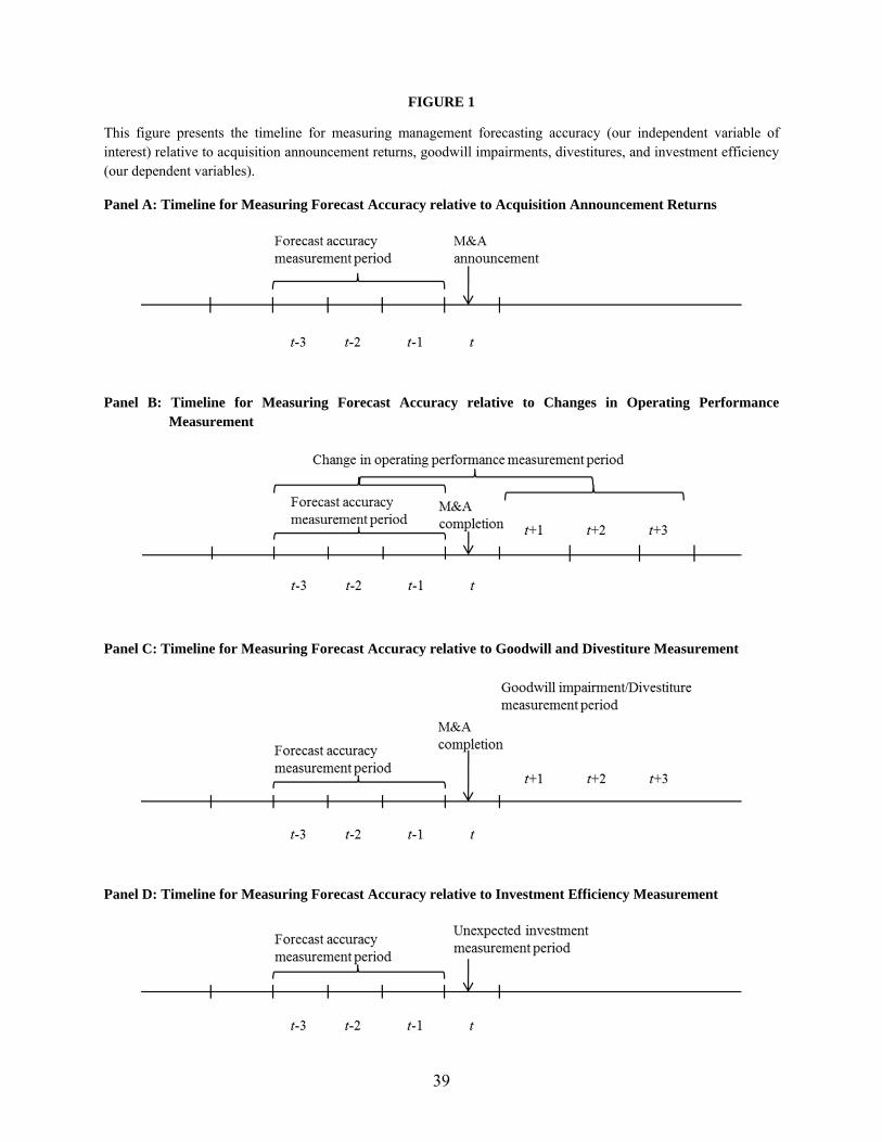
39

FIGURE 1

This figure presents the timeline for measuring management forecasting accuracy (our independent variable of interest) relative to acquisition announcement returns, goodwill impairments, divestitures, and investment efficiency (our dependent variables).

Panel A: Timeline for Measuring Forecast Accuracy relative to Acquisition Announcement Returns

Panel B: Timeline for Measuring Forecast Accuracy relative to Changes in Operating Performance

Measurement

Panel C: Timeline for Measuring Forecast Accuracy relative to Goodwill and Divestiture Measurement

Panel D: Timeline for Measuring Forecast Accuracy relative to Investment Efficiency Measurement

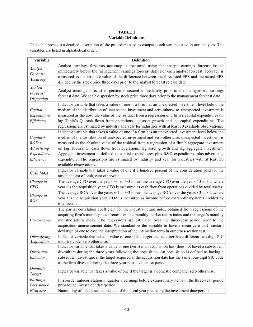
40

TABLE 1 Variable Definitions

This table provides a detailed description of the procedure used to compute each variable used in our analyses. The variables are listed in alphabetical order.

Variable Definition

Analyst Forecast Accuracy

Analyst earnings forecasts accuracy is measured using the analyst earnings forecast issued immediately before the management earnings forecast date. For each analyst forecast, accuracy is measured as the absolute value of the difference between the forecasted EPS and the actual EPS divided by the stock price three days prior to the analyst forecast release date.

Analyst Forecast Dispersion

Analyst earnings forecast dispersion measured immediately prior to the management earnings forecast date. We scale dispersion by stock price three days prior to the management forecast date.

Capital Expenditure Efficiency

Indicator variable that takes a value of one if a firm has an unexpected investment level below the median of the distribution of unexpected investment and zero otherwise. unexpected investment is measured as the absolute value of the residual from a regression of a firm’s capital expenditures on lag Tobin’s Q, cash flows from operations, lag asset growth and lag capital expenditures. The regressions are estimated by industry and year for industries with at least 30 available observations.

Capital + R&D + Advertising Expenditure Efficiency

Indicator variable that takes a value of one if a firm has an unexpected investment level below the median of the distribution of unexpected investment and zero otherwise. unexpected investment is measured as the absolute value of the residual from a regression of a firm’s aggregate investment on lag Tobin’s Q, cash flows from operations, lag asset growth and lag aggregate investment. Aggregate investment is defined as capital expenditures plus R&D expenditures plus advertising expenditure. The regressions are estimated by industry and year for industries with at least 30 available observations.

Cash M&A Indicator variable that takes a value of one if a hundred percent of the consideration paid for the target consist of cash, zero otherwise.

Change in CFO

The average CFO over the years t+1 to t+3 minus the average CFO over the years t-3 to t-1, where year t is the acquisition year. CFO is measured as cash flow from operations divided by total assets.

Change in ROA

The average ROA over the years t+1 to t+3 minus the average ROA over the years t-3 to t-1, where year t is the acquisition year. ROA is measured as income before extraordinary items divided by total assets.

Comovement

The partial correlation coefficient for the industry return index obtained from regressions of the acquiring firm’s monthly stock returns on the monthly market return index and the target’s monthly industry return index. The regressions are estimated over the three-year period prior to the acquisition announcement date. We standardize the variable to have a mean zero and standard deviation of one to ease the interpretation of the interaction term in our cross-section test.

Diversifying Acquisition

Indicator variable that takes a value of one if the target and acquirer have different two-digit SIC industry code, zero otherwise.

Divestiture Indicator

Indicator variable that takes a value of one (zero) if an acquisition has (does not have) a subsequent divestiture during the three years following the acquisition. An acquisition is defined as having a subsequent divestiture if the target acquired at the acquisition date has the same four-digit SIC code as the firm divested during the three-year post-acquisition period.

Domestic Target

Indicator variable that takes a value of one if the target is a domestic company, zero otherwise.

Earnings Persistence

First-order autocorrelation in quarterly earnings before extraordinary items in the three-year period prior to the investment date/period.

Firm Size Natural log of total assets at the end of the fiscal year preceding the investment date/period.

41

Forecasting Accuracy

Average accuracy of all annual management forecasts issued in the three years prior to the investment date/period (for acquisitions and capital expenditures, respectively). For each forecast, accuracy is measured as the absolute value of the difference between the management forecasted EPS minus the actual EPS divided by the stock price three days prior to the management forecast release date. The management forecast is either a point estimate or the mid-point of a range estimate of a firm’s annual earnings. Accuracy is multiplied by minus one to transform it in an increasing-in-quality measure.

Forecast Horizon

Average forecast horizon of all annual management forecasts issued in the three-year period prior to the investment announcement. For each forecast, forecast horizon is measured as the natural log of the number days between the forecast announcement date and the fiscal period end date.

Forecast Precision

Average precision of all annual management forecasts issued in the three-year period prior to the investment date/period. For each forecast, precision is measured as the absolute value of the difference between the upper bound of the management forecast minus the lower bound divided by the stock price three days prior to the management forecast release date. For a point forecast, the upper and lower bounds of the forecast range will be equal. Precision is multiplied by minus one to transform it in an increasing-in-precision measure.

Goodwill Impairment Indicator

Indicator variable that takes a value of one (zero) if a firm records (does not record) goodwill impairment losses in the three-year period following an acquisition that generates a large increase in goodwill. A large increase in goodwill is defined as an increase in goodwill greater or equal to 5% of total assets.

Goodwill Impairment Loss

The magnitude of goodwill impairment losses recorded in the three-year period following an acquisition that generates a large increase in goodwill. A large increase in goodwill is defined as an increase in goodwill greater or equal to 5% of total assets.

Growth Percentage change in sales in the fiscal year preceding the investment date/period. Hostile Takeover

Indicator variable that takes a value of one if the acquisition was classified as hostile in the SDC database, zero otherwise.

Leverage Leverage computed as the ratio of total liabilities to total assets at the end of the fiscal year preceding the investment date/period.

Market Adjusted CAR

Three-day cumulative abnormal return around the acquisition announcement. The abnormal return is computed as the stock return minus the return to the CRSP value-weighted index over the three day announcement window.

Market Model CAR

Three-day cumulative abnormal return around the acquisition announcement. The abnormal return is computed using the market model, where the parameters of the model are estimated over the window (-271,-21) trading days preceding the acquisition announcement and the market return is measured as the return to the CRSP value-weighted index.

No. of Bidders

Indicator variable that takes a value of one if there is more than one bidder for the target firm, zero otherwise.

Public Target Indicator variable that takes a value of one if the target is a public company, zero otherwise. Relative Target Size

Ratio of the acquisition transaction value to the acquirer’s market value.

Return on Assets (ROA)

Income before extraordinary items divided by lag total assets for the fiscal year preceding the investment date/period.

Stdev. ROA Standard deviation of quarterly ROA over the three years prior to the investment date/period. Stdev. Stock Returns

Standard deviation of the daily buy-and-hold stock returns measured over the one-year period prior to the investment date/period.

Stock M&A Indicator variable that takes a value of one if a hundred percent of the consideration paid for the target consist of the acquirer’s stock, zero otherwise.

Stock Returns Buy and hold stock return in the fiscal year preceding the investment date/period. For the acquisition announcement analysis, the buy and hold return is measured over the period (-13,-1) month relative to the acquisition announcement.

Tobin’s Q Market value of equity plus the book value of short and long term debt scaled by total assets measured at the end of the fiscal year preceding the investment date/period.

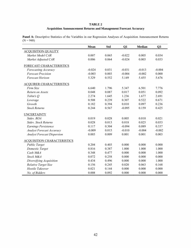
42

TABLE 2 Acquisition Announcement Returns and Management Forecast Accuracy

Panel A: Descriptive Statistics of the Variables in our Regression Analyses of Acquisition Announcement Returns (N = 948)

Mean Std Q1 Median Q3

ACQUISITION QUALITY Market Model CAR 0.007 0.065 -0.022 0.005 0.034 Market Adjusted CAR 0.006 0.064 -0.024 0.003 0.033

FORECAST CHARACTERISTICS Forecasting Accuracy -0.024 0.031 -0.031 -0.013 -0.004 Forecast Precision -0.003 0.003 -0.004 -0.002 0.000 Forecast Horizon 5.329 0.552 5.149 5.455 5.676

ACQUIRER CHARACTERISTICS Firm Size 6.640 1.796 5.347 6.501 7.776 Return on Assets 0.048 0.087 0.017 0.051 0.092 Tobin's Q 2.274 1.645 1.236 1.677 2.691 Leverage 0.508 0.239 0.307 0.522 0.671 Growth 0.182 0.394 0.010 0.097 0.236 Stock Returns 0.244 0.567 -0.095 0.159 0.425

UNCERTAINTY Stdev. ROA 0.019 0.028 0.005 0.010 0.021 Stdev. Stock Returns 0.028 0.013 0.018 0.025 0.033 Earnings Persistence 0.117 0.304 -0.094 0.089 0.337 Analyst Forecast Accuracy -0.009 0.015 -0.010 -0.004 -0.002 Analyst Forecast Dispersion 0.003 0.009 0.001 0.001 0.003

ACQUISITION CHARACTERISTICS Public Target 0.204 0.403 0.000 0.000 0.000 Domestic Target 0.816 0.387 1.000 1.000 1.000 Cash M&A 0.348 0.477 0.000 0.000 1.000 Stock M&A 0.072 0.258 0.000 0.000 0.000 Diversifying Acquisition 0.434 0.496 0.000 0.000 1.000 Relative Target Size 0.156 0.245 0.020 0.063 0.168 Hostile Takeover 0.021 0.144 0.000 0.000 0.000 No. of Bidders 0.008 0.092 0.000 0.000 0.000

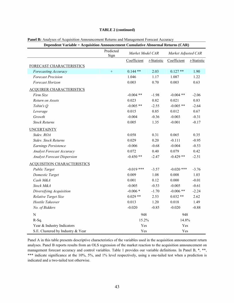
43

TABLE 2 (continued)

Panel B: Analyses of Acquisition Announcement Returns and Management Forecast Accuracy

Dependent Variable = Acquisition Announcement Cumulative Abnormal Returns (CAR)

Predicted

Sign Market Model CAR Market Adjusted CAR

Coefficient t-Statistic Coefficient t-Statistic

FORECAST CHARACTERISTICS

Forecasting Accuracy + 0.144 ** 2.03 0.127 ** 1.90

Forecast Precision 1.046 1.17 1.087 1.22

Forecast Horizon 0.003 0.70 0.003 0.63

ACQUIRER CHARACTERISTICS

Firm Size -0.004 ** -1.98 -0.004 ** -2.06

Return on Assets 0.023 0.82 0.021 0.83

Tobin's Q -0.005 ** -2.55 -0.005 ** -2.64

Leverage 0.015 0.85 0.012 0.67

Growth -0.004 -0.36 -0.003 -0.31

Stock Returns 0.005 1.35 -0.001 -0.17

UNCERTAINTY

Stdev. ROA 0.058 0.31 0.065 0.35

Stdev. Stock Returns 0.029 0.20 -0.111 -0.95

Earnings Persistence -0.006 -0.68 -0.004 -0.53

Analyst Forecast Accuracy 0.072 0.40 0.079 0.42

Analyst Forecast Dispersion -0.450 ** -2.47 -0.429 ** -2.51

ACQUISITION CHARACTERISTICS

Public Target -0.019 *** -3.57 -0.020 *** -3.76

Domestic Target 0.009 1.08 0.008 1.03

Cash M&A 0.001 0.12 0.000 -0.01

Stock M&A -0.005 -0.53 -0.005 -0.61

Diversifying Acquisition -0.006 * -1.70 -0.006 ** -2.24

Relative Target Size 0.029 ** 2.53 0.032 ** 2.62

Hostile Takeover 0.013 1.20 0.018 1.49

No. of Bidders -0.020 -0.85 -0.020 -0.88

N 948 948

R-Sq. 15.2% 14.8%

Year & Industry Indicators Yes Yes

S.E. Clustered by Industry & Year Yes Yes

Panel A in this table presents descriptive characteristics of the variables used in the acquisition announcement return analyses. Panel B reports results from an OLS regression of the market reaction to the acquisition announcement on management forecast accuracy and control variables. Table 1 provides our variable definitions. In Panel B, *, **, *** indicate significance at the 10%, 5%, and 1% level respectively, using a one-tailed test when a prediction is indicated and a two-tailed test otherwise.

44

TABLE 3 Analyses of Post-Acquisition Change in Operating Performance and Management Forecast Accuracy

Panel A: Descriptive Statistics of the Variables in our Analyses of Post-Acquisition Operating Performance (N=668)


ACQUISITION QUALITY Change in ROA -0.025 0.122 -0.052 -0.007 0.018 Change in CFO -0.004 0.085 -0.039 -0.005 0.034

FORECAST CHARACTERISTICS Forecasting Accuracy -0.025 0.030 -0.033 -0.014 -0.004 Forecast Precision -0.002 0.003 -0.003 -0.001 0.000 Forecast Horizon 5.308 0.576 5.066 5.440 5.684

ACQUIRER CHARACTERISTICS Firm Size 6.566 1.784 5.299 6.347 7.634 Return on Assets 0.048 0.091 0.018 0.053 0.092 Tobin's Q 2.348 1.728 1.249 1.712 2.814 Leverage 0.504 0.234 0.307 0.522 0.666 Growth 0.187 0.382 0.013 0.107 0.257 Stock Returns 0.253 0.604 -0.119 0.160 0.448

UNCERTAINTY Stdev. ROA 0.019 0.027 0.006 0.011 0.021 Stdev. Stock Returns 0.028 0.013 0.019 0.026 0.035 Earnings Persistence 0.119 0.307 -0.095 0.087 0.349 Analyst Forecast Accuracy -0.010 0.018 -0.010 -0.004 -0.001 Analyst Forecast Dispersion 0.003 0.005 0.000 0.001 0.003

ACQUISITION CHARACTERISTICS Public Target 0.193 0.395 0.000 0.000 0.000 Domestic Target 0.820 0.384 1.000 1.000 1.000 Cash M&A 0.329 0.470 0.000 0.000 1.000 Stock M&A 0.075 0.263 0.000 0.000 0.000 Diversifying Acquisition 0.433 0.496 0.000 0.000 1.000 Relative Target Size 0.158 0.247 0.018 0.063 0.182 Hostile Takeover 0.021 0.143 0.000 0.000 0.000 No. of Bidders 0.010 0.102 0.000 0.000 0.000

45

TABLE 3 (continued)

Panel B: Analyses of Post-Acquisition Operating Performance and Management Forecast Accuracy

Dependent Variable = Post Acquisition Change in Performance

Pr. Sign Change in ROA Change in CFO

Coefficient t-Statistic Coefficient t-Statistic


Forecasting Accuracy + 0.247 * 1.57 0.271 ** 1.71

Forecast Precision -1.880 -0.96 0.250 0.16

Forecast Horizon -0.002 -0.21 0.004 0.75


Firm Size 0.001 0.17 0.002 0.78

Return on Assets -0.422 *** -4.84 -0.248 *** -3.46

Tobin's Q -0.006 -1.36 -0.006 ** -2.07

Leverage 0.013 0.43 -0.008 -0.32

Growth -0.026 -1.57 0.009 0.69

Stock Returns 0.030 ** 2.31 0.015 ** 2.05

UNCERTAINTY

Stdev. ROA 1.032 ** 2.63 0.750 *** 2.68

Stdev. Stock Returns -1.515 *** -3.37 -0.233 -0.70

Earnings Persistence 0.002 0.10 0.007 0.55


Analyst Forecast Dispersion -4.023 -1.36 -0.968 -0.35


Public Target 0.001 0.07 0.004 0.38

Domestic Target -0.010 -0.97 -0.007 -0.71

Cash M&A -0.015 -1.34 -0.010 -1.37

Stock M&A -0.028 -1.16 -0.013 -0.71

Diversifying Acquisition -0.001 -0.07 0.004 0.57

Relative Target Size -0.017 -1.02 0.002 0.18

Hostile Takeover 0.027 1.10 -0.002 -0.09

No. of Bidders -0.009 -0.34 0.006 0.33

N 668 638

R-Sq. 27.7% 24.5%



Panel A in this table presents descriptive characteristics of the variables used in the analyses of post-acquisition changes in operating performance. Panel B reports results from OLS regressions of changes in post-acquisition operating performance on management forecast accuracy and control variables. Table 1 provides our variable definitions. In Panel B, *, **, *** indicate significance at the 10%, 5%, and 1% level respectively, using a one-tailed test when a prediction is indicated and a two-tailed test otherwise.

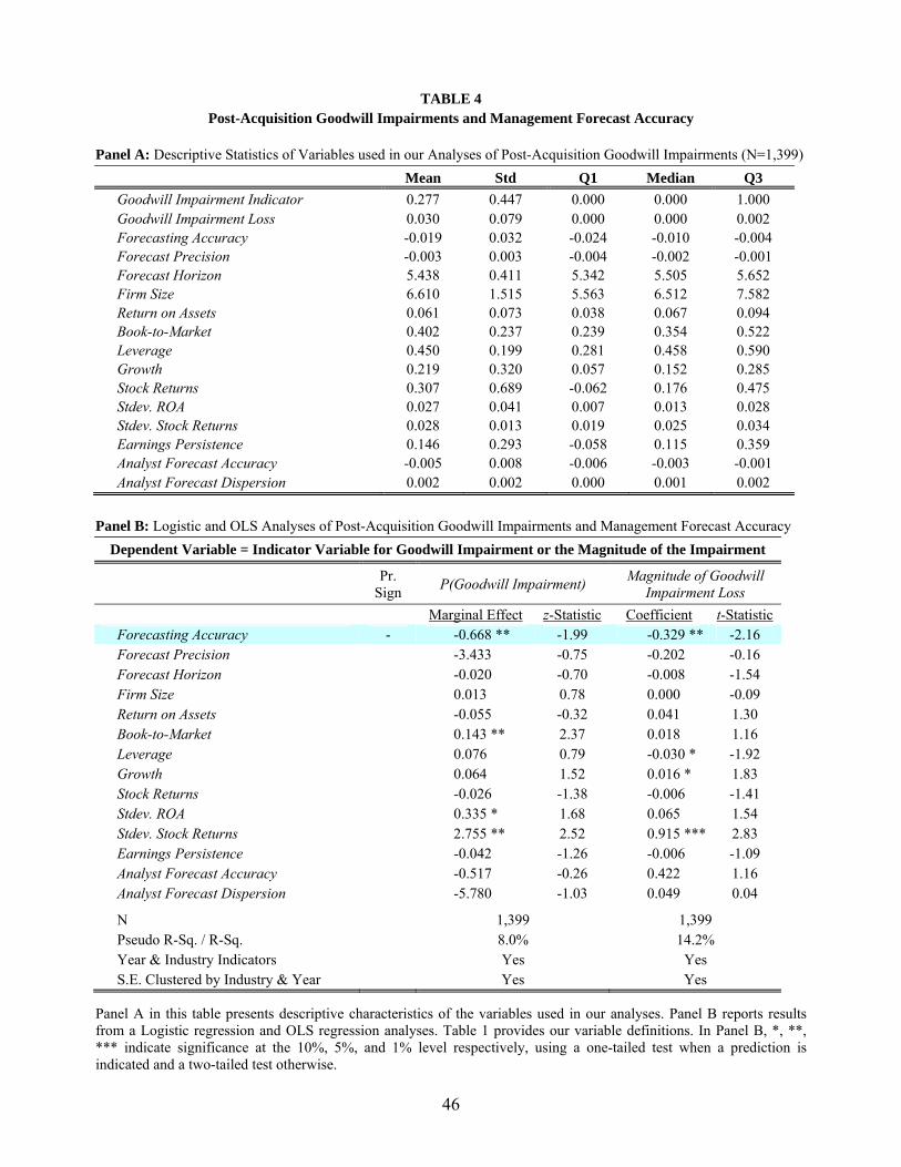
46

TABLE 4 Post-Acquisition Goodwill Impairments and Management Forecast Accuracy

Panel A: Descriptive Statistics of Variables used in our Analyses of Post-Acquisition Goodwill Impairments (N=1,399)


Goodwill Impairment Indicator 0.277 0.447 0.000 0.000 1.000 Goodwill Impairment Loss 0.030 0.079 0.000 0.000 0.002 Forecasting Accuracy -0.019 0.032 -0.024 -0.010 -0.004 Forecast Precision -0.003 0.003 -0.004 -0.002 -0.001 Forecast Horizon 5.438 0.411 5.342 5.505 5.652 Firm Size 6.610 1.515 5.563 6.512 7.582 Return on Assets 0.061 0.073 0.038 0.067 0.094 Book-to-Market 0.402 0.237 0.239 0.354 0.522 Leverage 0.450 0.199 0.281 0.458 0.590 Growth 0.219 0.320 0.057 0.152 0.285 Stock Returns 0.307 0.689 -0.062 0.176 0.475 Stdev. ROA 0.027 0.041 0.007 0.013 0.028 Stdev. Stock Returns 0.028 0.013 0.019 0.025 0.034 Earnings Persistence 0.146 0.293 -0.058 0.115 0.359 Analyst Forecast Accuracy -0.005 0.008 -0.006 -0.003 -0.001 Analyst Forecast Dispersion 0.002 0.002 0.000 0.001 0.002

Panel B: Logistic and OLS Analyses of Post-Acquisition Goodwill Impairments and Management Forecast Accuracy

Dependent Variable = Indicator Variable for Goodwill Impairment or the Magnitude of the Impairment

Pr.

Sign P(Goodwill Impairment)

Magnitude of Goodwill Impairment Loss

Marginal Effect z-Statistic Coefficient t-Statistic Forecasting Accuracy - -0.668 ** -1.99 -0.329 ** -2.16 Forecast Precision -3.433 -0.75 -0.202 -0.16 Forecast Horizon -0.020 -0.70 -0.008 -1.54 Firm Size 0.013 0.78 0.000 -0.09 Return on Assets -0.055 -0.32 0.041 1.30 Book-to-Market 0.143 ** 2.37 0.018 1.16 Leverage 0.076 0.79 -0.030 * -1.92 Growth 0.064 1.52 0.016 * 1.83 Stock Returns -0.026 -1.38 -0.006 -1.41 Stdev. ROA 0.335 * 1.68 0.065 1.54 Stdev. Stock Returns 2.755 ** 2.52 0.915 *** 2.83 Earnings Persistence -0.042 -1.26 -0.006 -1.09 Analyst Forecast Accuracy -0.517 -0.26 0.422 1.16 Analyst Forecast Dispersion -5.780 -1.03 0.049 0.04

N 1,399 1,399 Pseudo R-Sq. / R-Sq. 8.0% 14.2% Year & Industry Indicators Yes Yes S.E. Clustered by Industry & Year Yes Yes

Panel A in this table presents descriptive characteristics of the variables used in our analyses. Panel B reports results from a Logistic regression and OLS regression analyses. Table 1 provides our variable definitions. In Panel B, *, **, *** indicate significance at the 10%, 5%, and 1% level respectively, using a one-tailed test when a prediction is indicated and a two-tailed test otherwise.

47

TABLE 5 Post-Acquisition Divestitures and Management Forecast Accuracy

Panel A: Descriptive Statistics of the Variables used in our Analyses of Post-Acquisition Divestitures (N=5,051)


Divestiture Indicator 0.188 0.390 0.000 0.000 0.000 Forecasting Accuracy -0.021 0.027 -0.028 -0.012 -0.004 Forecast Precision -0.002 0.003 -0.003 -0.001 0.000 Forecast Horizon 5.408 0.479 5.283 5.495 5.680 Firm Size 7.370 1.874 6.046 7.236 8.557 Return on Assets 0.048 0.076 0.019 0.052 0.085 Book-to-Market 0.420 0.263 0.233 0.366 0.541 Leverage 0.524 0.221 0.358 0.529 0.671 Growth 0.217 0.365 0.040 0.129 0.284 Stock Returns 0.228 0.515 -0.068 0.151 0.393 Stdev. ROA 0.018 0.029 0.004 0.008 0.018 Stdev. Stock Returns 0.026 0.012 0.017 0.023 0.031 Earnings Persistence 1.572 0.655 1.069 1.614 2.054 Analyst Forecast Accuracy -0.008 0.033 -0.008 -0.003 -0.001 Analyst Forecast Dispersion 0.002 0.009 0.000 0.001 0.002

Panel B: Analyses of Post-Acquisition Divestitures and Management Forecast Accuracy

Dependent Variable = Probability of Post-Acquisition Divestiture

Predicted Sign Marginal Effect z-Statistic Forecasting Accuracy - -0.543 ** -1.77 Forecast Precision 6.701 ** 2.32 Forecast Horizon 0.016 0.81 Firm Size 0.061 *** 10.98 Return on Assets -0.106 -1.01 Book-to-Market 0.018 0.55 Leverage -0.057 -1.08 Growth 0.018 1.05 Stock Returns -0.005 -0.49 Stdev. ROA 0.092 0.72 Stdev. Stock Returns 0.665 0.80 Earnings Persistence 0.011 1.12 Analyst Forecast Accuracy -0.863 ** -2.27 Analyst Forecast Dispersion 0.325 0.49

N 5,051 Pseudo R-Sq. 14.8% Year & Industry Indicators Yes S.E. Clustered by Industry & Year Yes

Panel A in this table presents descriptive characteristics of the variables used in the post-acquisition divestiture analyses. Panel B reports results from a Logistic regression of the probability of divestiture post acquisition on management forecast accuracy and control variables. Table 1 provides our variable definitions. In Panel B, *, **, *** indicate significance at the 10%, 5%, and 1% level respectively, using a one-tailed test when a prediction is indicated and a two-tailed test otherwise.

48

TABLE 6 Cross-Section Test for Acquisitions Announcement Returns and Management Forecasting Accuracy

Dependent Variable = Acquisition Announcement CAR

Pr. Sign Coefficient t-Statistic Coefficient t-Statistic


Forecasting Accuracy + 0.296 *** 2.81 0.135 ** 2.16

Diversifying Acquisition -0.012 ** -1.96 -0.007 -1.50

Forecasting Accuracy × Diversifying Acq. - -0.423 ** -2.09 --- ---

Comovement --- --- 0.000 -0.15

Forecasting Accuracy × Comovement + --- --- 0.123 *** 2.39

Forecast Precision 1.050 1.45 1.033 1.38

Forecast Horizon 0.002 0.62 0.002 0.53


Firm Size -0.004 ** -2.00 -0.004 * -1.77

Return on Assets 0.017 0.69 0.021 0.85

Tobin's Q -0.005 ** -2.50 -0.004 ** -2.33

Leverage 0.011 0.75 0.013 0.74

Growth -0.004 -0.42 -0.003 -0.24

Stock Returns 0.006 1.28 0.007 1.37

UNCERTAINTY

Stdev. ROA 0.083 0.49 0.055 0.33

Stdev. Stock Returns -0.051 -0.19 -0.022 -0.08

Earnings Persistence -0.005 -0.57 -0.006 -0.66


Analyst Forecast Dispersion -0.545 *** -3.71 -0.413 *** -3.23


Public Target -0.018 ** -2.63 -0.018 ** -2.46

Domestic Target 0.010 1.49 0.010 1.20

Cash M&A 0.000 0.02 0.001 0.26

Stock M&A -0.006 -0.54 -0.006 -0.53

Relative Target Size 0.030 *** 3.20 0.029 *** 3.01

Hostile Takeover 0.013 1.33 0.011 0.95

No. of Bidders -0.015 -0.78 -0.022 -1.06

N 948 889

R-Sq. 15.5% 15.7%



This table presents the results from an OLS regression of acquisition announcement returns on management forecast accuracy, an interaction between management forecast accuracy and (i) an indicator variable for acquisitions within the same industry and (ii) comovement between the acquirer’s stock returns and target’s industry stock returns and control variables. Table 1 provides our variable definitions. In Panel B, *, **, *** indicate significance at the 10%, 5%, and 1% level respectively, using a one-tailed test when a prediction is indicated and a two-tailed test otherwise.

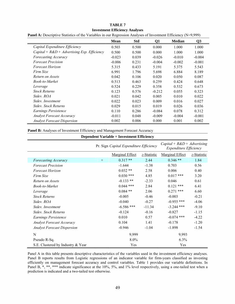
49

TABLE 7 Investment Efficiency Analyses

Panel A: Descriptive Statistics of the Variables in our Regression Analyses of Investment Efficiency (N=9,999)


Capital Expenditure Efficiency 0.503 0.500 0.000 1.000 1.000 Capital + R&D + Advertising Exp. Efficiency 0.500 0.500 0.000 1.000 1.000 Forecasting Accuracy -0.023 0.039 -0.026 -0.010 -0.004 Forecast Precision -0.006 0.231 -0.004 -0.002 -0.001 Forecast Horizon 5.315 0.433 5.191 5.375 5.543 Firm Size 6.991 1.796 5.698 6.884 8.189 Return on Assets 0.042 0.106 0.020 0.050 0.087 Book-to-Market 0.513 0.463 0.259 0.424 0.648 Leverage 0.524 0.229 0.358 0.532 0.673 Stock Returns 0.123 0.576 -0.212 0.055 0.323 Stdev. ROA 0.021 0.042 0.005 0.010 0.022 Stdev. Investment 0.022 0.023 0.009 0.016 0.027 Stdev. Stock Returns 0.029 0.015 0.019 0.026 0.036 Earnings Persistence 0.110 0.286 -0.084 0.078 0.312 Analyst Forecast Accuracy -0.011 0.048 -0.009 -0.004 -0.001 Analyst Forecast Dispersion 0.002 0.006 0.000 0.001 0.002

Panel B: Analyses of Investment Efficiency and Management Forecast Accuracy

Dependent Variable = Investment Efficiency

Pr. Sign Capital Expenditure EfficiencyCapital + R&D + Advertising

Expenditure Efficiency

Marginal Effect z-Statistic Marginal Effect z-Statistic

Forecasting Accuracy + 0.317 ** 2.44 0.346 ** 1.84 Forecast Precision -1.644 -1.38 0.703 0.56 Forecast Horizon 0.032 ** 2.58 0.006 0.40 Firm Size 0.030 *** 4.85 0.017 *** 3.20 Return on Assets -0.133 ** -2.33 0.046 0.61 Book-to-Market 0.044 *** 2.84 0.121 *** 6.41 Leverage 0.084 ** 2.06 0.271 *** 6.60 Stock Returns -0.005 -0.46 -0.003 -0.21 Stdev. ROA -0.040 -0.27 -0.955 *** -4.06 Stdev. Investment -6.586 *** -11.34 -3.244 *** -9.10 Stdev. Stock Returns -0.124 -0.16 -0.827 -1.15 Earnings Persistence 0.010 0.57 -0.074 *** -4.22 Analyst Forecast Accuracy 0.104 1.41 -0.178 -1.20 Analyst Forecast Dispersion -0.946 -1.04 -1.898 -1.54

N 9,999 9,993 Pseudo R-Sq. 8.0% 6.3% S.E. Clustered by Industry & Year Yes Yes

Panel A in this table presents descriptive characteristics of the variables used in the investment efficiency analyses. Panel B reports results from Logistic regressions of an indicator variable for firm-years classified as investing efficiently on management forecast accuracy and control variables. Table 1 provides our variable definitions. In Panel B, *, **, *** indicate significance at the 10%, 5%, and 1% level respectively, using a one-tailed test when a prediction is indicated and a two-tailed test otherwise.

management forecast quality and capital investment decisions

Documents