malte j. rasch, arthur gretton, yusuke murayama, wolfgang...

99:1461-1476, 2008. First published Dec 26, 2007; doi:10.1152/jn.00919.2007 J NeurophysiolK. Logothetis Malte J. Rasch, Arthur Gretton, Yusuke Murayama, Wolfgang Maass and Nikos

You might find this additional information useful...

47 articles, 15 of which you can access free at: This article cites http://jn.physiology.org/cgi/content/full/99/3/1461#BIBL

including high-resolution figures, can be found at: Updated information and services http://jn.physiology.org/cgi/content/full/99/3/1461

can be found at: Journal of Neurophysiologyabout Additional material and information http://www.the-aps.org/publications/jn

This information is current as of July 5, 2009 .

http://www.the-aps.org/.American Physiological Society. ISSN: 0022-3077, ESSN: 1522-1598. Visit our website at (monthly) by the American Physiological Society, 9650 Rockville Pike, Bethesda MD 20814-3991. Copyright © 2005 by the

publishes original articles on the function of the nervous system. It is published 12 times a yearJournal of Neurophysiology

on July 5, 2009 jn.physiology.org

Dow

nloaded from

http://jn.physiology.org/cgi/content/full/99/3/1461#BIBL

http://jn.physiology.org/cgi/content/full/99/3/1461

http://www.the-aps.org/publications/jn

http://www.the-aps.org/

http://jn.physiology.org

Inferring Spike Trains From Local Field Potentials

Malte J. Rasch,1 Arthur Gretton,2 Yusuke Murayama,2 Wolfgang Maass,1 and Nikos K. Logothetis2,3

1Institute for Theoretical Computer Science, Graz University of Technology, Graz, Austria; 2Max Planck Institute for BiologicalCybernetics, Tubingen, Germany; and 3Imaging Science and Biomedical Engineering, University of Manchester, Manchester,United Kingdom

Submitted 16 August 2007; accepted in final form 24 December 2007

Rasch MJ, Gretton A, Murayama Y, Maass W, Logothetis NK.Inferring spike trains from local field potentials. J Neurophysiol99: 1461–1476, 2008. First published December 26, 2007;doi:10.1152/jn.00919.2007. We investigated whether it is possible toinfer spike trains solely on the basis of the underlying local fieldpotentials (LFPs). Using support vector machines and linear regres-sion models, we found that in the primary visual cortex (V1) ofmonkeys, spikes can indeed be inferred from LFPs, at least withmoderate success. Although there is a considerable degree of variationacross electrodes, the low-frequency structure in spike trains (in the100-ms range) can be inferred with reasonable accuracy, whereasexact spike positions are not reliably predicted. Two kinds of featuresof the LFP are exploited for prediction: the frequency power of bandsin the high �-range (40–90 Hz) and information contained in low-frequency oscillations (�10 Hz), where both phase and power mod-ulations are informative. Information analysis revealed that bothfeatures code (mainly) independent aspects of the spike-to-LFP rela-tionship, with the low-frequency LFP phase coding for temporallyclustered spiking activity. Although both features and predictionquality are similar during seminatural movie stimuli and spontaneousactivity, prediction performance during spontaneous activity degradesmuch more slowly with increasing electrode distance. The generaltrend of data obtained with anesthetized animals is qualitativelymirrored in that of a more limited data set recorded in V1 ofnon-anesthetized monkeys. In contrast to the cortical field potentials,thalamic LFPs (e.g., LFPs derived from recordings in the dorsal lateralgeniculate nucleus) hold no useful information for predicting spikingactivity.

I N T R O D U C T I O N

In a typical electrophysiology experiment, the signal mea-sured by an electrode placed at a neural site represents themean extracellular field potential (mEFP) from the weightedsum of all current sinks and sources along multiple cells. If amicroelectrode with a small tip is placed close to the soma oraxon of a neuron, then the measured mEFP directly reports thespike traffic of that neuron and frequently that of its immediateneighbors as well. If the impedance of the microelectrode issufficiently low and its exposed tip is a bit farther from a singlelarge pyramidal cell, so that action potentials do not predom-inate the neural signal, then the electrode can monitor thetotality of the potentials in that region. The EFPs recordedunder these conditions are related both to integrative processes(dendritic events) and to spikes generated by several hundredneurons.

The two different signal types can be segregated by frequency-band separation. A high-pass filter cutoff of about 300–500 Hz

is used in most recordings to obtain multiple-unit spikingactivity (MUA), and a low-pass filter cutoff of about 300 Hz toobtain the so-called local field potentials (LFPs). Numerousexperiments have presented data indicating that such a bandseparation does indeed underlie different neural events (forreferences see, e.g., Logothetis 2003).

In summary, depending on the recording site and the elec-trode properties, the MUA most likely represents a weightedsum of the extracellular action potentials of all neurons withina sphere whose radius is about 140 to 300 �m, with theelectrode at its center (Henze et al. 2000). Spikes produced bythe synchronous firings of many cells can, in principle, beenhanced by summation and thus detected over a larger dis-tance (Arezzo et al. 1979; Huang and Buchwald 1977). Ingeneral, experiments have shown that large-amplitude signalvariations in the MUA range reflect large-amplitude extracel-lular potentials and that small-amplitude fast activity is corre-lated with small ones (Buchwald and Grover 1970; Gasser andGrundfest 1939; Grover and Buchwald 1970; Hunt 1951;Nelson 1966).

The low-frequency range (i.e., the LFPs) of the mEFPsignal, on the other hand, represents mostly slow events re-flecting cooperative activity in neural populations. Initiallythese signals were thought to represent exclusively synapticevents (Ajmone-Marsan 1965; Buchwald et al. 1965; Frommand Bond 1964, 1967). Evidence for their origin was oftengathered from current-source density (CSD) analysis and com-bined field potential and intracellular recordings (Mitzdorf1985; Nadasdy et al. 1998). Mitzdorf suggested that LFPsactually reflect a weighted average of synchronized dendroso-matic components of the synaptic signals of a neural popula-tion within 0.5–3 mm of the electrode tip (Juergens et al. 1999;Mitzdorf 1987). Later studies, however, provided evidence ofthe existence of other types of slow activity unrelated tosynaptic events, including voltage-dependent membrane oscil-lations (e.g., Kamondi et al. 1998) and spike afterpotentials.Taken together, LFPs represent slow waveforms, includingsynaptic potentials, afterpotentials of somatodendritic spikes,and voltage-gated membrane oscillations, that reflect the inputof a given cortical area as well as its local intracorticalprocessing, including the activity of excitatory and inhibitoryinterneurons.

Given the different natures of LFPs and MUA, we felt thatit would be interesting to address the question of whether onecan infer spiking of neurons from the locally measured fieldpotentials. Herein we address this question in a straightforward

Address for reprint requests and other correspondence: N. K. Logothetis,Max Planck Institute for Biological Cybernetics, Spemannstrasse 38, 72076Tubingen, Germany (E-mail: [email protected]).

The costs of publication of this article were defrayed in part by the paymentof page charges. The article must therefore be hereby marked “advertisement”in accordance with 18 U.S.C. Section 1734 solely to indicate this fact.

J Neurophysiol 99: 1461–1476, 2008.First published December 26, 2007; doi:10.1152/jn.00919.2007.

14610022-3077/08 $8.00 Copyright © 2008 The American Physiological Societywww.jn.org


Dow

nloaded from


manner. We use methods derived from the field of machinelearning in an attempt to infer exact spike timings from theunderlying LFPs. We compare the accuracy of spikes trainspredicted by supervised learning algorithms on a wide range ofrecordings from the primary visual cortex (V1) as well as fromthe lateral geniculate nucleus (LGN) of anesthetized and non-anesthetized macaques and investigate what kinds of featuresof the LFP are important for inferring spikes from LFP.

M E T H O D S

Data acquisition

Electrophysiological data recorded from nine anesthetized and twonon-anesthetized monkeys (Macaca mulatta) are included in thepresent study. All animal experiments were approved by the localauthorities (Regierungspraesidium) and are in full compliance withthe guidelines of the European Community (EUVD 86/609/EEC) forthe care and use of laboratory animals. Surgical procedures aredescribed elsewhere (Logothetis et al. 2002) together with hardwaredetails of the recording setup.

To perform the neurophysiological recordings in anesthetized mon-keys, the animals were anesthetized [remifentanil (typically 1�g �kg�1 �min�1)], intubated, and ventilated. Muscle relaxation wasachieved with mivacurium (5 mg �kg�1 �h�1). Body temperature waskept constant, and lactated Ringer solution was given at a rate of 10ml �kg�1 �h�1. During the entire experiment, the vital signs of themonkey and the depth of anesthesia were continuously monitored.Drops of 1% ophthalmic solution of anticholinergic cyclopentolatehydrochloride were instilled into each eye to achieve cycloplegia andmydriasis. Refractive errors were measured and contact lenses [hardpoly(methyl methacrylate) lenses by Wohlk Contactlinsen, Karlsruhe,Germany] with the appropriate dioptric power were used to bring theanimal’s eye into focus on the stimulus plane. Simultaneous recordingof neural activities were made from the primary visual cortex (V1)using 8–16 electrodes configured in 4 � 4 or 2 � 8 matrices in a gridof 1–2 mm. Electrode tips were typically (but not always) positionedin the upper or middle cortical layers. The impedance of the electrodevaried from 300 to 800 k�. In the case of simultaneous LGNrecording an additional set of drives, usually consisting of two to fourelectrodes, was additionally positioned. The electronic interface, in-

cluding drives, holder, and preamplifier, was custom designed tominimize cross talk of signals between electrodes (typically �1 ppm).The signals were amplified and filtered into a band of 1–8 kHz (AlphaOmega Engineering, Nazareth, Israel) and then digitized at 21 kHzwith 16-bit resolution (National Instruments, Austin, TX), ensuringenough resolution for both local field and spiking activities. Binocularvisual stimulation was provided through a two-fiber optic system(Avotec, Stuart, FL) after fine alignment to each of the animal’sfoveas by a modified retinoscope coupled with a stimulus projectorholder.

In the case of the anesthetized animals we differentiate between twodifferent conditions: spontaneous activity (“spo”) and movie-drivendata (“stm”). In the former the input screen is blank for about 5 min;in the latter a 4- to 6-min segment of a commercially available movieis shown. Movie frames were synchronized with the refresh rate of themonitor (60 Hz, two synchronizations per movie frame) and covered7–12° of the visual field. Most of the electrodes were confirmed tohave a receptive field within the movie presentation area (see Fig. 1Bfor an example). Multiple trials of movie presentations and spontane-ous activity are run within one recording session (intermingled withrecordings of other stimuli not considered here). From these data weinclude 1,304 recorded time series in the present study, which we calltrials throughout this article. The data set consisted of recordings fromnine animals collected in 12 recording sessions. From each session wetake five repeats of movie presentation and five repeats of spontaneousactivity trials (with the exception of j97nm1, where only one movietrial is available). To avoid any subjective selection bias all measuredelectrode channels per session are included. This results in 670 trialsfor spontaneous activity and 634 for movie stimulus recorded using134 electrode placements. Movies are identical within a session butmay differ between sessions.

In three sessions (two anesthetized monkeys) no more than fourelectrodes were simultaneously placed in the LGN. Thus stimulireflected in these data (100 trials) are exactly identical to those incorresponding recordings of the V1 data. This data is separated againaccording to the conditions spontaneous activity (“spo(L)”) andmovie-driven activity (“stm(L)”). Data from non-anesthetized mon-keys are more limited and were included in the present study only tocorroborate results for the data described earlier. They are recordedusing one to four tetrodes from chronic implants penetrating V1 (fora detailed description of surgical methods and recording setup see

25 30 35 40 45−5

0

5

Time [sec]

LFP

[SD

uni

ts]

−5 0 5

−10

−5

0

Visual field [°]

Vis

ual f

ield

[°]

Receptive fields

V1 electrode

LGN electrode

Stimulus region

0

200

400

600

Inst

. spi

ke r

ate

[Hz]

A B

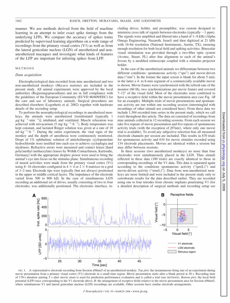
FIG. 1. A: representative electrode recording from Session a98nm5 of an anesthetized monkey. Top plot: the instantaneous firing rate of an experiment duringmovie presentation from a primary visual cortex (V1) electrode in a small time region. Movie presentation starts after a blank period at 30 s. Recording timeof 170-s duration starting 5 s after movie onset is used for prediction performance evaluation and is called a trial (see METHODS). Bottom plot: the local fieldpotential (LFP) trace corresponding to the V1 electrode above. B: the arrangement of receptive fields relative to the movie presentation area for Session a98nm5,where simultaneous V1 and lateral geniculate nucleus (LGN) recordings are available. Other sessions have similar electrode arrangements.

1462 RASCH, GRETTON, MURAYAMA, MAASS, AND LOGOTHETIS

J Neurophysiol • VOL 99 • MARCH 2008 • www.jn.org


Dow

nloaded from


Tolias et al. 2007) in a total of 56 trials. Unlike the data fromanesthetized animals the stimulus conditions here are mixed, withspontaneous activity (no task) and a fixation task showing gratings ofdifferent orientations. This last data is labeled “awake” in the follow-ing. All data are processed in the same way as outlined in the nextsection.

PROCESSING. The data preprocessing steps are as follows. Electrodesignals were decimated to 7 kHz. Spiking activity is inferred fromhigh frequencies of the resulting signal (see following text). Therecording hardware introduces a high-pass filter with a cutoff �1 Hz;1 Hz is thus the lowest frequency considered here.

The 7-kHz signal is low-pass filtered with a cutoff frequency of 250Hz and resampled first to 500 Hz for computational convenience. Theresulting signal is low-pass filtered at 90 Hz to derive local fieldpotentials (LFPs). For low-pass filtering we use a custom finiteimpulse response filter (FIR): a Kaiser window FIR filter with 60-dBattenuation in the stopband, a 0.01-dB passband ripple, and a transi-tion band of 1 Hz. To eliminate possible phase shifts, signals werefiltered forward and backward (using the MatLab filtfilt function). Thesignal is then resampled to a final sampling rate of 200 Hz.

Good properties of FIR filters are won at the expense of large filtersizes (a few seconds). However, since we discard leading and trailingportions of �15 s of each trial, filter on- and offset artifacts are of noconcern here.

SPIKE EXTRACTION. Spike times are detected by applying a thresh-old to the high-pass filtered 7 kHz signal described earlier (fourth-order Butterworth, cutoff frequency 500 Hz). Since this MUA signalis usually asymmetric, the detection threshold is automatically appliedto that side where spike waveforms exhibit greater deflection. Toavoid dependence of the size of spikes the threshold is applied at3.5SD (�) of the “noise component” of the MUA signal. � isestimated by calculating the SD of the signal, neglecting the 4.55%(�2�) absolute highest values divided by the percentage of variancethat is kept in general, when setting the probability of absolute values�2� to zero.

Visual inspection confirms that spikes are well detected. If theassumption of a Gaussian “noise component” is correct, then therate of wrongly detected spikes is about 1.6 Hz (for � � 3.5 SD).Note that the resulting spike trains will most likely include spikesfrom multiple neurons (see DISCUSSION). Because most recordingswere done with single-tip electrodes we do not use any kind of spikesorting.

Learning to infer spike trains

The learning algorithm has to learn to map from LFP waveforms(or other LFP features) to spikes. Ideally, the learning algorithmshould output all predicted real-valued spike timings at once if theLFP time course is given as input, although this task requires toomuch data. Instead, we simplify the task by assuming that spikes areindependent and that the spike-to-LFP relationship remains constantover time. With these assumptions one can use a binary classifier,which yields the prediction of a spike (or no spike) at time t.Concatenating the prediction for each t results in a predicted spiketrain for a given LFP. Note that the independence assumption does notimply that predicted spike trains are necessarily uncorrelated becausetemporal correlation can be induced by the underlying LFPs.

In supervised fashion the binary classifier is trained on a set oftraining examples and tested on a distinct test set. We train a binaryclassifier on LFP features summarized in the sample vectors xi, i �1, . . . , L, to predict the label yi � {1, �1}. The index i is the ith pointof the discrete LFP time series with sampling frequency 1/� atrecording time ti � i� t0. Thus yi � 1 states that there occurs (atleast) one spike within time bin ti and yi � �1 indicates no spike. Inthis framework prediction is temporally restricted to the samplingresolution of the LFPs, making it necessary to bin the spike timings.

The sampling interval � is 5 ms, in accordance with the samplingfrequency of the LFP signal (200 Hz).

LEARNING ALGORITHMS. A support vector machine (SVM) wasused (Vapnik 1999) as our learning algorithm. For a more detailedintroduction to SVMs see, for example, Bishop (2006), Burges(1998), and Scholkopf and Smola (2002). SVMs perform binaryclassification in a supervised fashion.

Briefly, the model can be stated as follows (for details see Bishop2006)

hx� � wT�x� � b (1)

where one looks for the decision boundary or weight vector w; b is abias term and � is a projection into a space of features. SVMs choosethe hyperplane that has the widest margin between both classes ratherthan an arbitrary separating hyperplane. This is achieved by enforcingappropriate constraints in the optimization. For nonseparable prob-lems, such as our real-world data, one introduces the concept of softmargins, i.e., in the optimization one now allows for incorrectlyclassified examples, where an additional parameter C regulates thepenalty.

SVMs have the power to do nonlinear separation (seen from theperspective of input space) by choosing an appropriate kernel thatimplicitly defines the feature map �. Herein nonlinear radial basisfunction (RBF) kernels are used.

As a simple alternative to SVMs we used standard linear regression(with a constant bias term) on the label vector and the samples (see,e.g., Bishop 2006). Briefly, using a linear model hreg(xi) � wTxi bwe calculated the optimal weight vector w* by minimizing the meansquared error [hreg(xi) � yi]

2� on the training samples. Class labels onthe test set were obtained by thresholding with the sign function, i.e.,yj � sign [h*reg(xj)].

EXTRACTION OF LFP FEATURES. An LFP feature could be any aspectof the LFP that one might deem helpful for inferring whether there isa spike at ti. In our analysis, we used the LFP at different lags withrespect to ti, its power at different frequencies, and the phase ofoscillations at particular frequencies (also at different lags). Multiplefeatures are simply concatenated in the sample vector xi. Note thateach dimension of the resulting samples {xi} is normalized to zeromean and unit SD. Features are extracted prior to dividing the samplesinto test and training sets.

If g(ti) represents the (normalized) voltage at sampling bin ti, a timefeature may be defined as Tk(ti) :� g(tik), where � � k� representsthe time lag (we neglect boundaries to simplify the description).Features Tk(ti) simply represent the LFP time course relative to sampletime ti.

Another type of feature, which we denote Pf,k(ti), is the estimatedpower at (center) frequency f of the LFP time course at time tik. Toobtain an estimate for the power at a given frequency and time, wecalculated the spectrogram, using the multitaper approach introducedby Thomson (Jarvis and Mitra 2001; Percival and Walden 2002;Thomson 1982). Because spikes are single events on the timescale of�, we chose a high temporal resolution at the expense of frequencyresolution. We set the moving window to 150 ms and the time–bandwidth product to 1.6, which implicitly sets the half-bandwidth toW � 10.67 Hz. Spectral estimation was averaged over two Slepiantapers. Because this window setting does not allow accurate powerestimation �20 Hz we used larger windows for bands �20 Hz (500ms) and �6 Hz (2 s). This reduced the half-bandwidth to 3.2 and 0.8Hz for frequencies �20 and 6 Hz, respectively. We also tried Morletwavelets with variable bandwidth per frequency, but this did not alterprediction performance.

To access phase information at particular frequencies of the LFP,we first band-pass filtered the recorded signal with the FIR Kaiserfilter (described earlier) with a bandwidth of 2 (Fig. 6) or 4 Hz (Fig.7), and then used the Hilbert transform to extract an instantaneous

1463INFERRING SPIKE TRAINS FROM LFPS



Dow

nloaded from


phase �f(ti) at frequency f. From these signals we defined phasefeatures �f,k(ti) :� cos [�f(tik)] having a lag of � � k�. Thesefeatures have phase information identical to that of the band-passedsignals but are devoid of any amplitude modulation (AM). Addition-ally, we used �f,k :� sin [�f(tik)] in the feature analysis of Fig. 6 tohelp the classifier linearly extract phase locking at phases where thecosine would be near the zero crossing.

PERFORMANCE MEASURES. The kappa measure was used as a mea-sure of performance (Cohen 1960). Let pl,r be the fraction of sampleshaving target label l � {�1, 1} and predicted label r � {�1, 1} andlet ql and qr be the fraction of samples in the test set that have the labell in the target or the label r in the prediction, respectively. Then thechance level for classification is given by c � q�1q�1 q1q1. If wedefine 0 � p�1,�1 p1,1 to be the overall fraction of correctlyclassified samples (both positive and negative), then is given by

:�0 � c

1 � c

(2)

This measure is a normalized above-chance classification rate. It canbe easily seen that equals zero if prediction is at chance level (i.e.,0 � c) and equals one if the predicted classification is perfect (i.e.,0 � 1).

Another performance measure is the Spearman rank correlation r�

between smoothed predicted spike trains and target spike trains. Thismight give a more intuitive picture of the prediction quality. If notstated otherwise, spike trains are smoothed by a Gaussian kernel ofwidth 25 ms.

Yet another measure for prediction quality is the mutual informa-tion between class labels. The mutual information (MI) between targetspikes S and the prediction outcome of a classifier C(F) using LFPfeatures F and labels L :� {�1, 1} is

I�S;CF �� l�L

�r�L

PI,r log2

pl,r

qlqr

(3)

where we take the probabilities defined earlier. This estimation of MIis different from nonparametric approaches in that it can accessdependence that is only in reach of the classifier; thus one has to makesure that the classifier captures the main aspects of its dependence.Note that we use the naive estimator for mutual information [withoutbias correction (Panzeri et al. 2007)]. Since all MI value calculationsinvolve an identical number of bins—that is, two, one for eachclass—we can nevertheless safely compare results even for classifi-cations with different numbers of features. However, the absolute MIvalues might be biased.

To access redundancy, synergy, and independence of information(Pola et al. 2003; Schneidman et al. 2003) conveyed by two featuresF1 and F2 about the spiking activity S, we estimate mutual informationusing two classifiers trained on features F1 and F2 individually,yielding I(S; F1):� I[S; C(F1)] and I(S; F2) :� I[S; C(F2)]. Then a thirdclassifier is trained on both features jointly, yielding I(S; F1, F2) :�I[S; C(F1, F2)]. If both features carried independent information fromthe perspective of the classifier, both features together would conveyidentical information as individual features; i.e., I(S; F1, F2) � I(S;F1) I(S; F2). If both features were related by a one-to-one mapping(completely redundant information about the spikes), then all termswould be equal: I(S; F1) � I(S; F2) � I(S; F1, F2). If the two featuresdid not carry information individually, i.e., I(S; F1) � I(S; F2) � 0, butcarried information together, I(S; F1, F2) � 0, they would be termed(completely) synergistic. Thus we define a normalized degree ofsynergy of information about the spikes (as measured by the classi-fication algorithm) as (Schneidman et al. 2003)

syn F1, F2 �S� :�IS; F1, F2� � IS; F1� � IS; F2�

IS; F1, F2�(4)

This measure ranges from �1 in the case of completely redundantinformation to 1 for completely synergic information. The measuresyn (F1, F2 � S) is zero if both features F1 and F2 convey independentinformation about the spikes S.

To analyze prediction accuracy on different timescales, we usedspectral coherence (Jarvis and Mitra 2001). Spectra were again esti-mated via a multitaper approach designed for point events (Jarvis andMitra 2001). Here the time–bandwidth product was set to TW � 3using the average of K � 5 tapers, yielding a half-bandwidth of W �0.001 Hz for T � 17 s.

PERFORMANCE EVALUATION. We evaluated the prediction perfor-mance for each trial separately, using 10-fold cross-validation. Weanalyzed a 170-s region, avoiding the on- and offset of the moviestimulus. Spontaneous activity trials are also restricted to 170-sduration. In the case of tetrode recordings, performance is estimatedas the average performance of the four wires of the tetrode.

Hyperparameters for the SVM algorithm were estimated as follows.The RBF kernel width was selected by a heuristic procedure. Wetook to be 1.77 (or 3.54) times the median distance of all Euclideandistances in the training set. For each trial we chose that C (and )showing the best performance (averaged over 10 cross-validation runson a logarithmic grid of 25 values from 0.25 to 400). We visuallyconfirmed that this range is appropriate for our data (not shown). Weused the libSVM library (http://www.csie.ntu.edu.tw/�cjlin/libsvm/)for all SVM calculations.

Since the sample sizes were heavily biased toward the negative(nonspiking) class we randomly picked approximately the same num-ber of samples of both classes from the training region. This effec-tively changes the loss function from equal loss to higher importancefor spikes (about a fivefold increase, depending on the mean firingrate). We used 1,000 and 1,200 samples for spiking and nonspikingclasses (or the maximum available in the training region with aconstant class ratio) and empirically found this to be a good compro-mise between prediction quality and computational speed because�1,000 samples only marginally improved the results (not shown).Training the classifier on all possible samples was prohibitive due tothe enormous sample size. We tried to use class biasing in the Cparameters (Musicant et al. 2003), but this only increased computationtime with little gain in prediction quality.

The test set was always a temporally contiguous region to avoidfeature correlation of trained and tested samples that might lie nearbyin time if a randomized set of samples were used.

FEATURE SELECTION ALGORITHM. We now describe how to deter-mine the usefulness of different features for spike prediction. Al-though features important for the SVM classifier are hard to interpret,in the case of linear regression (with squared loss) one can derive ananalytical expression for the prediction error of a set of featuresinvolving only the STAs and correlation among features. Based onthis prediction error, we derived an algorithm that forwardly selects asmall subset of features out of a much larger pool of features. Assubsequently explained, the selected subset will show minimal pre-diction error compared with other subsets with the same number offeatures. In that sense the subset of features selected by our algorithmrepresents the most useful features from a given pool. Because thisfeature selection can be efficiently done for huge feature pools, werestricted feature analyses to linear classification, rather than using theSVM classifier. This is not too restrictive in our case because linearclassification achieves almost 90% of the performance of an SVMclassifier (see RESULTS).

In linear regression we look for the weight vector w that hasminimal error in a mean squared sense




Dow

nloaded from


�w� � yi � wTxi�2� (5)

where the brackets indicate averaging over all samples i. Minimizingthe error is straightforward and results in the optimal weight vector1

w* of

w* � xixiT��1 yixi� (6)

provided that the estimated correlation matrix A: � xixiT� has full

rank. We note that we have a binary classification and thus yi � {�1,1}. Thus

yixi� � �c�1

c1 � c�1

m�1 �c1

c1 � c�1

m1

where m�1 and m1 are the class means for the nonspiking and spikingclass, respectively, and c�1 and c1 are the number of samples in eachclass. With the condition that each feature is normalized to varianceone and zero mean, Eq. 6 reduces to

w* � cA�1m1 (7)

with

c :�2c1

c1 � c�1

The minimal error is then given by

�w*� � 1 � c2m1TA�1m1 (8)

In other words, the error of the linear regression is dependent only onthe STA m1 and the correlation among features. We note that if werestrict ourselves to the use of n features (the dimensions of xi) out ofa pool of N � n features, the preceding equations remain valid if thecorrelation matrix and the mean are also restricted to these featuresonly (that is, A has size n � n with rank n and m1 is n-dimensional).

To select a set of n important features we use the following iterativealgorithm. We start with the feature that has the highest STA, i.e., f1 �arg maxj � (m1)j � (the variance of each feature being normalized toone). Assume now that n � 1 features are already selected. Then wesearch through all N � n 1 remaining features and choose one thatminimizes the error (Eq. 8), where the restriction of the correlationmatrix is now enforced on the n features rather than on n � 1 (andanalogously with m1). We stop this iteration when the desired numberof features m �� N is selected.

This algorithm is highly efficient in finding a good set of features,since we need to calculate the correlation matrix only between theselected features and all other features (which costs much less effortthan calculating it for all pairs).

R E S U L T S

This section is organized as follows. After showing thegeneral spike-to-LFP relationships present in our data, wereport the population performance for the task of predictingspike trains from LFP, focusing first on data from V1 ofanesthetized monkeys (nine monkeys) collected during thepresentation of 5 min of commercial movie stimuli and equallylong periods of spontaneous activity. We then compare theseresults with a more limited set of sessions recorded from V1 ofawake monkeys (two monkeys) and with results on data fromLGN of anesthetized monkeys (two monkeys). Finally, we

investigate which LFP features are important for the predictiontask and which aspect of the spikes they code for.

Average spike to LFP-power and -phase relation

Figure 1 shows spiking activity and (normalized) LFPs of arepresentative electrode. Relationships between spiking activ-ity and underlying LFPs are visualized in Fig. 2.

In Fig. 2A the spike-triggered average (STA) of the LFPs ofan example electrode during movie stimulus is plotted. Clearly,there is a linear relation between spikes and LFPs. One notes asharp negativity at spike position at zero time lag and aprominent upswing for positive time lags, i.e., after spiking hasoccurred. Likewise, in the STA of the spectrogram (Fig. 2B)power is enhanced in the high-frequency range (40–90 Hz)during spiking activity. Enhancement of power at high LFPfrequencies as a response to spikes is common among elec-trodes, stimulus conditions, and monkeys, as we will see in thenext sections.

Figure 2C shows the probability of spiking activity at theoscillation phase of a particular LFP frequency for the sameexample electrode, but averaged �30 repeats of the movie pre-sentation (�120 min of recording time). One notes that the phasesof all LFP frequencies are at least weakly related to spikingactivity (Raleigh test of nonuniform angular distribution). Moststrikingly, spikes are relatively tightly locked to phases of lowfrequencies ( 10 Hz). The generality of this behavior isillustrated in Fig. 2D, where the phase preferred by spikes isplotted as an average across all data from V1 (anesthetizedanimals). The average preferred phase shifts with frequencyfrom the onset of a positive half-wave to the valley of the LFPoscillation (compare with Fig. 2E). This behavior is veryconsistent, regardless of whether activity is spontaneous ormovie-driven. For some electrodes the preferred phase-fre-quency dependence is slightly different (as in the example ofFig. 2C for high frequencies). For a few electrodes the phase-to-spike relation seems to be mirrored at � (not shown).

The gray-shaded area in Fig. 2D shows the (average) phaserange within which 50% of the spikes fall. It would be zero forperfect phase locking and � for no phase–spike relation. Onenotes that this range is somewhat smaller for low frequencies(0.85�), but approaches 0.98� for frequencies �20 Hz, indi-cating that the phase locking is far from perfect at all frequen-cies and is especially weak for high frequencies.

In summary, we have seen that there is indeed a consistentrelationship between LFPs and spiking activity on average. Inthe next sections we ask to what degree it is possible to exploitthese relations (and maybe other information available in theLFP) in a systematic way to infer spikes from the LFP.

Population prediction performance

In Fig. 3 a typical example of a predicted spike train isdepicted together with the used LFP features. Figure 3, A andB shows 8 s of LFP spectrogram and the time course in the testregion, respectively. Small vertical lines in Fig. 3B indicatespike times before binning to 5-ms resolution. Several inter-esting points can be noted. As expected from the LFP-to-spikerelations discussed in the last section, spikes preferentiallyoccur in the upswing and valleys of very low and medium LFPoscillations, as seen for instance at times 171 and 173.4 s in

1 Note that the optimal weight vector w* has only minimal error for theregression, and that there may be a better weight vector for classification. Weneglect this here for the sake of simplicity.




Dow

nloaded from


Fig. 3B. Additionally, the power of multiple frequencies isenhanced when a burst of spiking activity occurs, as suggestedby Fig. 2B, but the frequency response to bursts is diffuse andvariable (compare the burst at 173.4 s to that at 174.5 s). Theclustering of spiking activity on a timescale of a few hundredmilliseconds in this example is actually quite typical in our V1data (see following text). For the single spikes in between theclusters no feature of the LFP is immediately predictive.

Figure 3C shows target and predicted spiking activities.Prediction of spikes is made for individual sample times at aresolution of 5 ms using a set of LFP time course and fre-quency features (see following text). Concatenating the predic-tion over time yields a predicted spike train that is comparedwith the target spike train. One notes that the predictioncaptures, at least approximately, the overall structure of thespike train. The occurrence of bursts of spiking activity, whichare associated with easily seen traces in the LFP time courseand spectrogram, is well predicted. Nevertheless, the exactonsets and offsets of the bursts are somewhat inaccurate in theprediction. Even some smaller bursts and single spikes are

closely predicted (172.5 s), although no clear mark in the LFPtime course or spectrogram can be seen with the naked eye.However, their length (176.6 s) and exact position (176.3 s)sometimes seem inaccurate. There are also occasions wherespikes are simply missed (172.9 s) or fabricated (173.9 s).

Prediction performance is evaluated in different ways. Onemeasure is the performance, a measure defined on thesamples in the test set, which is positive for above-chance classi-fication; it equals one for perfect classification (see METHODS

for definitions). In contrast, the correlation measure r� (seeMETHODS) is defined as a local average in the time domain andis therefore less sensitive to small temporal inaccuracies. Theperformance measure of the predicted spike train in Fig. 3C hasa value of � 0.40, which is relatively good (but not the bestpossible; see following text). Rank correlation is r25 ms � 0.60.

In the example of Fig. 3, the predicted spike train resemblesthe original to a certain degree. We ask whether this predictionquality carries over to LFPs recorded from different monkeys,electrodes, and stimulus conditions. For that we estimatedprediction performance using a large data set (see METHODS).

−1 −0.5 0 0.5 1

−0.4

−0.2

0

0.2

0.4

0.6

Time lag [sec]

Nor

mal

ized

LF

P [S

DU

]

LFP−STAShuffled spikes SD

Time lag [sec]

Fre

quen

cy [H

z]

−2 0 20

20

40

60

80N

ormalized LF

P pow

er [SD

U]−0.1

0

0.1

0.2

0.3

0.4

Spike probability [%

]

1.8

1.9

2

2.1

2.2

2.3

movie

spont

100

101

102

0

1

2

3

4

5

6

Pha

se o

f LF

P [r

ad]

Frequency [Hz]

−1 0 1

0 20 40 60 800

1

2

3

4

5

6

Frequency [Hz]

Pha

se o

f LF

P [r

ad]

A B

C D E

FIG. 2. Spike–LFP relationships for one electrode in V1 of an anesthetized monkey during movie stimulation (A–C) and across all recordings from V1 inanesthetized monkeys (D and E). A: spike-triggered average (STA) LFP. For significance levels interspike intervals (ISIs) are shuffled and the SD of the resultingSTA is calculated. B: STA of the LFP spectrogram (see METHODS), with power series normalized to zero mean and unit SD. Power at high frequencies is clearlymodulated by spiking activity, whereas power at lower frequencies shows only diffuse dependence on spikes. C: probability distribution of LFP phases at aparticular spiking position. LFP phases are computed via Hilbert transform (1-Hz bands). Here all spikes over 30 repeats of movie-driven activity are included(same electrode as before). Note that the color map shows only a narrow range of probabilities and that values above or below the limits are truncated. Blackdots indicate the preferred (i.e., mean) phase. No phase locking of spikes would result in a uniform distribution at 2% per bin. Although locking to low frequenciesis strong, locking to high frequencies is only weak (but present). D: the average preferred phases for all electrodes across all anesthetized data individually formovie-driven activity (“movie”) and spontaneous activity (“spont”). Bars indicate SEs. The phase range containing half of the spikes around the preferred phaseis indicated by the shaded area. E: the interpretation of phase, showing that spikes are locked at very low frequencies to the onset of a positive half-wave andat high frequencies to the valley.




Dow

nloaded from


Inferences are made on the basis of a set of LFP features, withwhich we observed a dependence between spikes and LFPs inthe previous section. In the population analysis we include asfeatures the time course around each sample position (in awindow of 100 ms before and 300 ms after spike position) andan estimate of the frequency content of LFPs at zero time lag[Pf,0(ti); see METHODS], resulting in a total of 116 features. Thisfeature set generally produced good performance (with a rea-sonable computational speed) over a wide range of data. Forthe prediction itself a nonlinear support vector machine is usedwith radial basis functions such as kernel (SVM–RBF) anda linear classification is employed (for details see METHODS).

In Fig. 4 the prediction performance over all trials is eval-uated (on 10 cross-validation runs) and averaged. The anesthe-tized V1 data set is labeled “spo” for spontaneous activity and“stm” for movie stimulus-driven activity. We shall focus onthese data for the moment. The remaining conditions shown inthis plot are discussed in the following text.

Plot A shows the average performance for the SVM–RBFclassifier and for linear classification. From the results we drawthe following insights. First, since performance measure is�0 for above-chance prediction it can be said that bothclassifiers can exploit information in the LFP time course to

predict spiking activity (all conditions highly significant; t-test,P � 10�6, Wilcoxon signed-rank test for zero median, P �10�6). Second, prediction quality for the stimulus conditionand for spontaneous activity differs only slightly: indeed, onecannot reject the hypothesis that the underlying distributionshave identical means (two-sided unpaired t-test, P � 0.21;linear, P � 0.18). However, if one compares pairwise record-ings during spontaneous activity and stimulus presentationdone with identical electrodes, mean and median predictionperformances on spontaneous activity are significantly betterthan those on stimulus-driven activity (one-sided paired t-test:P � 10�4; linear, P � 10�4; for the distribution-free Wilcoxonmatched-pairs signed-ranks test: P � 10�4; linear, P � 10�3).Average prediction performance for spontaneous activity is � 0.211 � 0.006 (linear � 0.185 � 0.005) and �0.201 � 0.005 (linear � 0.175 � 0.005) for stimulus-drivenactivity.

Third, nonlinear margin classification is consistently betterthan linear classification (one-sided paired t-test: “stm” P �10�6, “spo” P � 10�6; Wilcoxon matched-pairs signed-rankstest, P � 10�6). It amounts to an increase, on average, of about12% in performance. This suggests that the mapping from LFPfeatures is nonlinear. However, since a simple linear regression

171 172 173 174 175 176 177

0

100

200

300

Time [s]

Rat

e [s

pike

s/s]

A

B

C

Fre

quen

cy [H

z]

0

20

40

60

80

Target SDF (σ=0.01s)Prediction (κ=0.40)

−4

−2

0

2

4

Vol

tage

[SD

U]

LFP and spikes

Normalized power

−2 0 2 4 6 8 10

FIG. 3. Example of spike prediction from LFP (anesthetized monkey, Session a98nm5, spontaneous activity). A: the (normalized) spectrogram of the 8 s ofLFP activity. B: corresponding LFP time course and spiking activity. Spikes are indicated by marks before binning to the LFP resolution (5 ms). C: the binnedtarget spikes and their spike density function (blue) together with the predicted spikes and their spike density function (red). The prediction is relatively good( � 0.40, r25 ms � 0.60) on this trial, but other trials show even better performance (compare with r25 ms values of other trials in Fig. 4B, “spo”). One notesthat regions of high activity are well predicted, whereas the location of single spikes is less accurate. Classification is done with the support vector machine (SVM)radial basis function (RBF) classifier trained on the region 35–160 s using the same features as for the population analyses (Fig. 4).




Dow

nloaded from


classifier already achieves almost 90% of the accuracy of thenonlinear classifier, one could state that the LFP feature spaceexploited here seems expressive enough for this task.

We found that for individual trials performance varieswidely. For selected trials prediction performance can reach � 0.65. Plot B of Fig. 4 shows the rank-correlation measurer25 ms of the SVM–RBF prediction. Each thin short line repre-sents performance for an individual trial. Whereas the corre-lation for some trials is as high as 0.8–0.9 on this moderatelysmall timescale (25 ms), it is almost zero in others. There aresome trials where prediction fails completely in each of theconditions. The failing trials are not all from the same sessionssince the session means (markers) tend to cluster around theoverall mean.

There is not much variability in performance over time: theaverage SD for the performance of five repeats of 170-msrecordings for the same electrodes is 0.023 � 0.002 forstimulus-driven activity, 0.026 � 0.002 for spontaneous activ-ity, and 0.045 � 0.002 for both together. This is in contrast tothe variance across electrodes recorded simultaneously. Herethe average SD (in ) is 0.113 � 0.004 for stimulus-driven and0.130 � 0.005 for spontaneous activity. The roughly 25-foldincrease in variance across electrodes compared with within-electrode variance suggests that prediction performance is amatter of which electrode is being observed, rather than stim-ulus condition or time. Electrode tips might be positioned in aregion where the arrangement of current sources and sinksmight differ (e.g., in deep or superficial layers), or where active

0 2 4 6 8 100

20

40

60

80

Rel

ativ

e pe

rfor

man

ce κ

/κ0m

m [%

]

Electrode distance [mm]

stm ± SEspo ± SE

−3.3%mm−1+44%

−0.2%mm−1+43%

0

0.05

0.1

0.15

0.2

0.25A

vg. κ

per

form

ance

LFP: V1 Spikes: V1

LGNV1

V1LGN

LGNLGN

Electrode configuration

Same electrode (stm)Cross electrodes (stm)Same electrode (spo)Cross electrodes (spo)Significant performanceNot significant

A B

C D

stm spo awake stm (L) spo (L)0

0.05

0.1

0.15

0.2

0.25

0.3

0.35

Condition

Avg

. κ p

erfo

rman

ce

SVM RBFLinear regression

stm spo awake stm (L) spo (L)0

0.2

0.4

0.6

0.8

1

Condition

Ran

k co

rrel

atio

n [σ

=25

ms]

a98nm5a98nm6c98nm1c98nm2d04nm1d04nm2d98atg02nm1g97nm1georgios3j97nm1l97nm1r97nm1s02nm1

FIG. 4. Population performance for spike prediction from LFP. A: average prediction performance for SVM and the linear regression classifier acrossconditions [anesthetized monkey V1, movie stimulus (“stm”), anesthetized monkey V1, spontaneous activity (“spo”), non-anesthetized monkey V1 with mixedstimuli (“awake”), and spontaneous activity or movie-stimulus driven activity in anesthetized monkeys from LGN, “spo (L)” and “stm (L),” respectively].Prediction is above chance level for all conditions (see RESULTS for significance tests). B: prediction accuracy of the nonlinear classifier evaluated by rankcorrelation between target and predicted spikes train smoothed by a Gaussian kernel of width � � 25 ms. Red horizontal lines indicate the average performancewithin each condition and its SE. Small black lines show the quality on individual trials. In some cases prediction yields very accurate results, with correlationsas high as 0.8–0.9. Black curves on the sides of each condition are smoothed histograms over trials. Symbols indicate the average performance of individualsessions (i.e., 1 day of recording). Average session performance clusters near the overall mean, but variance for individual electrodes is high. C: cross-electrodeprediction. LFPs are taken from one electrode and spikes from another. Relative prediction decreases much faster with increasing electrode distance in the “stm”condition than for the “spo” condition. A linear fit of the data points is also shown. Vertical lines indicate SEs. D: average prediction performance forsimultaneous LGN and V1 recordings (3 sessions, 2 monkeys). Performance is compared for available cross-electrode prediction from different areas and withaverage performance when using the same electrode for spikes and for LFPs. X-axis labels indicate where LFP and spikes originate from.




Dow

nloaded from


neurons might be less well correlated with the bulk activity ofthe cortex. Since we cannot distinguish the layers from whichelectrodes record, we cannot pursue this further.

Up to now we have presented results for recordings onlyfrom V1 of anesthetized monkeys. We also have a limitedamount of data available from V1 where monkeys were notanesthetized and free to behave. The stimuli for this data set(labeled “awake”) are mixed and include spontaneous activityand fixation tasks. Another pool of data consists of recordingsfrom LGN of anesthetized monkeys (labeled “stm(L)” and“spo(L)”; see METHODS).

We see from Fig. 4A that prediction differs quite drasticallyfor the different data types. Spike prediction for the anesthe-tized monkey data from V1 is more than fivefold better thanthat in the LGN, where performance is hardly above chance: onaverage, � 0.035 � 0.005 (linear � 0.033 � 0.005) formovie-driven activity and � 0.027 � 0.003 (linear �0.022 � 0.003) for spontaneous activity.

As in V1, there is little difference between spontaneous andmovie-driven activity in LGN, although there is a reversedtendency for spike prediction to be easier on movie-drivenactivity than that on spontaneous activity. This tendency isbarely significant (one-sided paired t-test: P � 0.02; linear,P � 0.01; Wilcoxon matched-pairs signed-ranks test: P �0.05; linear, P � 0.08).

We find that average prediction performance on awake datais � 0.063 � 0.005 (linear � 0.046 � 0.005). This is muchworse than that on anesthetized V1 data (unpaired t-test, P �10�5), but still significantly better than that on LGN data (allunpaired one-sided t-test, P � 0.05). Figure 4B reveals thatindividual trials have a correlation of target and predictionsimilar to that in anesthetized monkeys. There are trials withcorrelation up to r25 ms � 0.6, whereas in the case of the LGN,no trial exceeds 0.3 correlation.

Cross-electrode predictions

The volume of cortex that contributes to the generation of LFPsis different from that producing our spiking signal (see INTRODUCTION).Thus it might be interesting to see how the relationship be-tween the two signals changes with distance. Because record-ings were done simultaneously with multiple electrodes (in thedata set from anesthetized animal), we tried to infer spikesfrom LFPs collected with two different electrodes. In Fig. 4Cthe average performance is plotted against the (three-dimen-sional) distance of the electrode tips. To facilitate comparison,performance is evaluated relative to the average performanceachieved using the spiking signal from the electrode fromwhich the LFPs were taken.

One notes that prediction performance drops to about 40%when electrodes are 1 mm apart (the minimal distance in ourrecording setup). Interestingly, for stimulus-driven activityperformance degrades significantly with distance (rank corre-lation between distance and relative kappa performance usingall measurements: �0.20, P � 10�4), whereas for spontaneousactivity no significant correlation with distance can be foundfor distances 1 cm (rank correlation 0.015, P � 0.2). Notethat the number of samples becomes relatively small fordistances �6 mm since rectangular electrode grids with 1-mmspacing are used for most sessions. However, we can safely

compare spontaneous and stimulus-driven activity because theelectrode placements do not change with the condition.

Because LGN data were collected while other electrodessimultaneously recorded from V1, we can investigate whetherthe LFPs of V1 can be predicted on the basis of spikes fromLGN and vice versa. This is shown in Fig. 4D averaged overdata from the three sessions recording simultaneous measure-ments from V1 und LGN (see METHODS). Performance isaveraged either across electrode predictions (regardless ofdistances) or over all predictions using the same electrode forboth signals. Although results are difficult to interpret becauseof the limited size of the data set, one notes that using LFPsfrom LGN and spikes from V1 results in performance abovechance, whereas LFPs from V1 seem to hold no informationabout spikes in LGN (unpaired Wilcoxon signed-rank test formedian performance different from zero, significance level 0.05).

Temporal accuracy of predicted spike trains

We found an average value of about 0.2, which is wellabove chance but nevertheless far from perfect prediction at � 1. On the other hand, in example Fig. 3C some features ofthe target spike trains seem to be well captured by the predic-tion, especially regions of high and low activity, which alter-nate on a timescale of about 0.5 s in this example. Thus onemight ask at what timescale the predicted spiking activity mostclosely resembles the target spiking activity or at what timingaccuracy the prediction fails.

To answer this we evaluated the coherence between targetand predicted spike train (Fig. 5). Coherence is a correlationmeasure in the frequency domain. Coherence at a particularfrequency makes a statement about the exactness of the pre-diction on a timescale of one over that frequency. We alsoestimated the temporal accuracy directly in the time domain(by varying the correlation kernel width) where one arrives atsimilar conclusions (not shown).

1 10 1000

0.2

0.4

0.6

0.8

1

Frequency [Hz]

Coh

eren

ce

5ms10ms25ms100ms500ms

stmspoawakestm (L)spo (L)

FIG. 5. Coherence levels of predicted and target spike trains. Coherence isplotted against frequency and is averaged over all trials for each condition. Forcomparison we included surrogate data, in which spike trains were generatedwith the same ISI distribution as in the monkey data. Gray dashed lines showcoherence between surrogate spike train and its jittered version with Gaussiannoise of different SDs (� from 5 to 500 ms, as listed in the plot). Coherencedrops for higher frequencies, suggesting that, on average, prediction is reason-ably good only for slow structure in the spike trains. Note that the chancecoherence level is at about 0.15 here, as shown by the surrogate data. Chancelevels do not tend to zero because coherence is estimated on 10 cross-validation regions (each 17-s duration) and only subsequently averaged overall trials. Colored areas indicate SEs.




Dow

nloaded from


In Fig. 5 one observes that coherence is low for highfrequencies and rises for low frequencies. Thus the generalresemblance of a predicted spike train might be adequate, butthe exact spike position is often predicted with some jitter. Thisis also evident in the example of Fig. 3.

Coherence drops at about 25 Hz for the anesthetized V1data. This timescale is comparable to a spike train whosespikes are jittered by Gaussian random noise with SD of 25 ms.Coherence levels of such surrogate data are indicated by thedashed lines in Fig. 5. Since the jitter destroys all informationin the high frequencies, the plateau at low coherence for thesurrogate data can be taken as a significance level for thecoherence estimation. In surrogate data low-frequency aspectsstay completely intact (thus a coherence of 1), but for predictedspike trains this is only partly the case. However, averagecoherence rises considerably for larger timescales comparedwith smaller ones, suggesting that at least in a subset of trials,slow structure is well predicted.

Data from the non-anesthetized monkey are less coherent atlow frequencies but much more so than for data from LGN,where almost no significant coherence is observed, even forlow frequencies. Note that we have far fewer trials from LGNand non-anesthetized V1, so averaging is less effective insmoothing.

In summary, predicted spike trains are seldom accurate to aspike timing precision of �25 ms, as suggested by comparisonto a jittered version of the original spike train. On the otherhand, predicted spike trains capture structure on a largertimescale reasonably well, say for clusters of high spikingactivity in the 100-ms range.

LFP features important for inferring spikes

For determining the usefulness of particular LFP features forinferring spiking activity, we iteratively select a small numberof features out of a large pool of possible features. The selectedsubset shows minimal prediction error for a given number offeatures, and therefore selected features can be seen as the mostimportant for prediction. Because spike prediction in LGN isalmost impossible, only V1 data are analyzed in the following.

We consider a feature pool consisting of phase and powerfeatures (Pf,k, �f,k, and �f,k). Phase is estimated on 45 frequencybands each 2 Hz wide, whereas the power features Pf,k havedifferent frequency resolutions (see METHODS). Setting k appro-priately, we include time lags of 3s in both directions (beforeand after ti). Out of this pool of features, containing togetherN � 138,115 features, only up to m � 10 features are selectedfor each trial individually using the algorithm outlined inMETHODS. Figure 6D shows that, on average, selecting only 10features out of the huge pool is enough for a linear classifier toapproach the performance of the linear classifier used previ-ously (Fig. 4), which used 116 general features (dashed line).For the first five selected features the gain in performance ishighest.

Figure 6, A–C shows histograms of m � 5 selected, mostimportant features aggregated for all trials. Phase- and power-related features are colored blue and red, respectively. Analo-gous to previous results, useful features differ only slightlybetween stimulus-driven activity (Fig. 6A, “stm”) and sponta-neous activity (Fig. 6B, “spo”): stimulus induction does notseem to induce a general change in the preference of features

for spike–LFP interaction. One notes that in both spontaneousand stimulus-driven activity power fluctuations in the high�-band (40–90 Hz) are preferred features. Selected frequenciesare biased toward high values, with 80–90 Hz being the mostlikely selection. Indeed, high-frequency power features areselected as the first and most useful feature in about 90% of thetrials (and in 82% in non-anesthetized animals; not shown).The time lags of the selected � power features are almostsymmetrically distributed around zero (with a small bias to-ward positive lags) in a zone spanning about 50 ms to eitherside. There are smaller symmetrical peaks at 150 ms, whichmay be attributed to the power estimation, where we use amoving window of 150-ms duration. Likewise peaks at 80 and60 Hz are introduced by spectral estimation because the band-width is roughly 20 Hz (see METHODS).

We identified low-frequency information as a second classof useful LFP features, in particular phase information oflow-frequency bands �10 Hz. Time lags of selected phasefeatures are mostly positive, meaning that the time of thefeature is most informative after the spike. Useful lags varyfrom �50 to 200 ms, depending on the frequency, and they canbe as long as 500 ms for the lowest frequency bands ( 2 Hz).Time lags vary according to an oscillation period of the lowbands. Power modulations in the low-frequency bands areselected about as often. The time lags of these features aredistributed widely, which is caused by the long window settingof 2 s needed to estimate power at low frequencies (seeMETHODS).

Bands from 10 to 40 Hz, especially 15 to 30 Hz, seem to bemuch less important for inferring spikes. Despite a smallnumber of scattered features in the “spo” condition, phaseinformation for �-bands (e.g., �40 Hz) does not play a role,either.

For the non-anesthetized animals results are hard to inter-pret, given the limited amount of data (see Fig. 6C). However,it seems that the overall structure is similar to the V1 data ofanesthetized monkeys in having high-frequency power featuresas well as very low frequency phase features for positive lags.However, there seems to be an increase of selected powerfeatures for intermediate frequencies.

Both feature types, meaning high-frequency power featuresaround zero lag and low-frequency information, either low-frequency power or low-frequency phase features with positivelags, are often jointly selected among the five optimizedfeatures. This shows that individual trials have similar features.We found that in 75% (“stm”), 59% (“spo”), and 72%(“awake”) of the trials both types of features are jointlyselected, more specifically a high-frequency power feature (�40Hz) with absolute lags of �250 ms and a low-frequency phasefeature (�10 Hz) with positive lags or a low-frequency powerfeature �10 Hz. In absolute terms high-frequency powers arepreferred over low-frequency features (“stm” 61 vs. 24%;“spo” 62 vs. 19%; “awake” 47 vs. 24%). In “stm” and “spo”conditions low-frequency phase features with positive lags areselected slightly more often in combination with high gammapowers than low-frequency power features (“stm” 49 vs. 44%;“spo” 38 vs. 33%), whereas low-frequency powers are pre-ferred in the awake condition (28 vs. 60%). Neither of thelow-frequency features is present in about 25% of the trialswhen the first 5 selected features are considered, although this




Dow

nloaded from


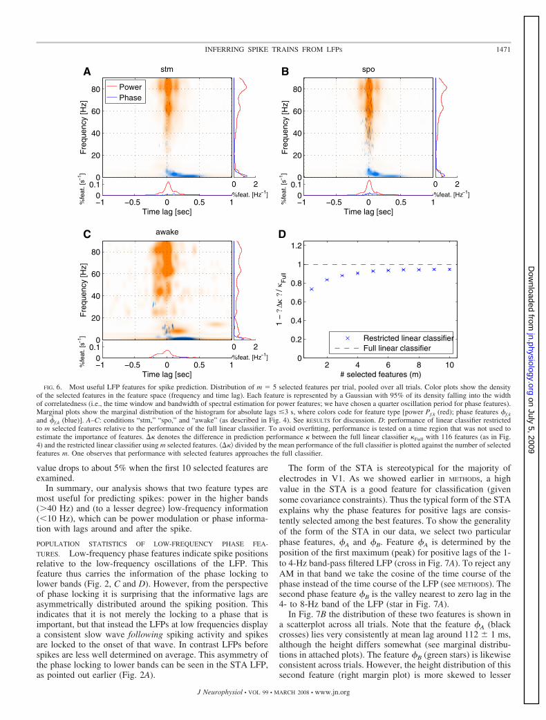
value drops to about 5% when the first 10 selected features areexamined.

In summary, our analysis shows that two feature types aremost useful for predicting spikes: power in the higher bands(�40 Hz) and (to a lesser degree) low-frequency information(�10 Hz), which can be power modulation or phase informa-tion with lags around and after the spike.

POPULATION STATISTICS OF LOW-FREQUENCY PHASE FEA-

TURES. Low-frequency phase features indicate spike positionsrelative to the low-frequency oscillations of the LFP. Thisfeature thus carries the information of the phase locking tolower bands (Fig. 2, C and D). However, from the perspectiveof phase locking it is surprising that the informative lags areasymmetrically distributed around the spiking position. Thisindicates that it is not merely the locking to a phase that isimportant, but that instead the LFPs at low frequencies displaya consistent slow wave following spiking activity and spikesare locked to the onset of that wave. In contrast LFPs beforespikes are less well determined on average. This asymmetry ofthe phase locking to lower bands can be seen in the STA LFP,as pointed out earlier (Fig. 2A).

The form of the STA is stereotypical for the majority ofelectrodes in V1. As we showed earlier in METHODS, a highvalue in the STA is a good feature for classification (givensome covariance constraints). Thus the typical form of the STAexplains why the phase features for positive lags are consis-tently selected among the best features. To show the generalityof the form of the STA in our data, we select two particularphase features, �A and �B. Feature �A is determined by theposition of the first maximum (peak) for positive lags of the 1-to 4-Hz band-pass filtered LFP (cross in Fig. 7A). To reject anyAM in that band we take the cosine of the time course of thephase instead of the time course of the LFP (see METHODS). Thesecond phase feature �B is the valley nearest to zero lag in the4- to 8-Hz band of the LFP (star in Fig. 7A).

In Fig. 7B the distribution of these two features is shown ina scatterplot across all trials. Note that the feature �A (blackcrosses) lies very consistently at mean lag around 112 � 1 ms,although the height differs somewhat (see marginal distribu-tions in attached plots). The feature �B (green stars) is likewiseconsistent across trials. However, the height distribution of thissecond feature (right margin plot) is more skewed to lesser

spo

Fre

quen

cy [H

z]

0

20

40

60

80

0 2 %feat. [Hz−1]

−1 −0.5 0 0.5 10

0.1

Time lag [sec]

%fe

at. [

s−1 ]

awake

Fre

quen

cy [H

z]

0

20

40

60

80

0 2 %feat. [Hz−1]

−1 −0.5 0 0.5 10

0.1

Time lag [sec]

%fe

at. [

s−1 ]

2 4 6 8 100

0.2

0.4

0.6

0.8

1

1.2

# selected features (m)

1 −

? ∆κ

? / κ

Ful

l

Restricted linear classifierFull linear classifier

A B

C D

0 2 %feat. [Hz−1]

−1 −0.5 0 0.5 10

0.1

Time lag [sec]

%fe

at. [

s−1 ]

stm

Fre

quen

cy [H

z]

0

20

40

60

80 PowerPhase

FIG. 6. Most useful LFP features for spike prediction. Distribution of m � 5 selected features per trial, pooled over all trials. Color plots show the densityof the selected features in the feature space (frequency and time lag). Each feature is represented by a Gaussian with 95% of its density falling into the widthof correlatedness (i.e., the time window and bandwidth of spectral estimation for power features; we have chosen a quarter oscillation period for phase features).Marginal plots show the marginal distribution of the histogram for absolute lags 3 s, where colors code for feature type [power Pf,k (red); phase features �f,k

and �f,k (blue)]. A–C: conditions “stm,” “spo,” and “awake” (as described in Fig. 4). See RESULTS for discussion. D: performance of linear classifier restrictedto m selected features relative to the performance of the full linear classifier. To avoid overfitting, performance is tested on a time region that was not used toestimate the importance of features. � denotes the difference in prediction performance between the full linear classifier Full with 116 features (as in Fig.4) and the restricted linear classifier using m selected features. �� divided by the mean performance of the full classifier is plotted against the number of selectedfeatures m. One observes that performance with selected features approaches the full classifier.




Dow

nloaded from


values than for feature �B, suggesting that it might be lessuseful for prediction. There is also a minority of trials in whichneither feature was well expressed, indicated by the scatteredoutliers.

INFORMATION CONVEYED BY LOW-FREQUENCY BANDS AND HIGH-

FREQUENCY POWER FEATURES. To compare information con-veyed by different features about spikes we use the mutualinformation between target spikes train and predicted spikestrain (see METHODS). Mutual information between the classlabels is a lower bound for the mutual information containedbetween the signals under consideration (Natschlager andMaass 2005). It is only a lower bound, since a classificationmethod might fail to use all the information contained in thesignal. However, it is unlikely that a nonlinear SVM classifierwould miss much of the dependence in our data, since therelationship between features and spikes seems to be mostlysimple proportionality. Recall that for our data a linear classi-fier already achieves about 90% of the performance of anonlinear classifier.

First, we tested prediction performance for single-frequencypower and low-phase features individually using the SVMclassifier. In Fig. 7C we show the average information aboutthe spikes at different frequencies for V1 of anesthetizedmonkeys (blue crosses). The information change with fre-

quency closely resembles the number of selected power fea-tures per frequency from our selection algorithm in the previ-ous section. We note that, on average, frequencies around 80Hz convey the most information about the spikes. If one usesall the features tested here simultaneously, average perfor-mance reaches 0.037 � 0.002 bits, which is 35% higher thanthat when the best individual feature is used.

Information contained in the power decreases monotonicallywith frequency. This decrease can also be seen on the level ofindividual trials (not shown). If one uses either one of thelow-frequency phase features �A and �B on its own, informa-tion drops to about a third for �A and much lower for �Bcompared with that of the best power feature (black and greenlines in Fig. 7C, respectively). Despite the usefulness of low-frequency power modulation in combination with high-frequencypowers (as shown in the feature selection), low-frequency powerexhibits poorer performance as a single feature than the phasefeatures (in particular in comparison to �A; see Fig. 7C). Note thatthe timing resolution of the phase features is much higher asphase is defined at any moment in time, whereas power has tobe estimated within a window of sufficient length. The inducedtemporal correlation of nearby time points for the low-fre-quency power seems to be too high to predict spike times onits own.

−0.2 0 0.2 0.40

500

Time lag [sec]

# T

rials

0 20 40 60 800

0.005

0.01

0.015

0.02

0.025

0.03

Mut

ual I

nfor

mat

ion

[bits

]

I (S; P

f)

I (S; φA)

I (S; φB)

φ

A

φB

φA

φB

Syn

ergy

of i

nfor

mat

ion

−1

−0.8

−0.6

−0.4

−0.2

0

Frequency [Hz]

Fre

quen

cy [H

z]

20 40 60 80

20

40

60

80

BA

C D

−2 −1 0 1 2

−0.5

0

0.5

1

Time lag [sec]

Nor

mal

ized

LF

P [S

DU

]

STA 1−90HzShuffled SDφ−STA 1−4Hzφ−STA 4−8Hz

Feature φA

Feature φB

−0.5

0

0.5

Nor

mal

ized

LF

P [S

DU

]

0 100 200 300# Trials

Frequency [Hz]

FIG. 7. Information about spiking activity conveyed by phase features and frequency power features. A: STA. LFP STA (blue line) as well as the STA forthe 1- to 4-Hz (black line) and 4- to 8-Hz (green line) band-pass filtered LFP. In the latter cases all power modulation is discarded (see METHODS), yielding purelyphase related signals. The definitions of phase features �A (black cross) and �B (green star) are indicated. B: distribution of lags of features �A and �B for alltrials of the anesthetized V1 data. C: information about spikes conveyed by single features. D: redundancy of information about spikes conveyed by anycombination of LFP features. Color coding indicates the amount of information synergy (see METHODS, Eq. 4). See RESULTS for discussion.




Dow

nloaded from


We next investigated the information conveyed by any twofeatures jointly. If two LFP features F1 and F2 conveyedindependent information about spiking activity S, the normal-ized measure for synergy of information syn (F1, F2 � S) (Eq. 4)would be zero. In general, this measure ranges from minus onefor completely redundant information to one for completelysynergistic information (for details see METHODS). Figure 7Dshows the average normalized synergy of information aboutthe spikes for all combinations of features. Here synergy ofinformation is calculated on the basis of single trials, wheretrials having joint information not significantly above zeroinformation are excluded (Wilcoxon signed-rank test, P value�0.1). Generally, information conveyed by high-frequencybands is mainly independent from information contained inlow-frequency bands. The information in individual high-power features is more redundant [e.g., for 87 and 50 Hz,syn (P50 Hz, P87 Hz � S) � �0.40 � 0.02] than between high-power features and phase features, where information is nearlyindependent [synergy values with high-frequency power fea-tures around �0.2; for instance, syn (�A, P81 Hz � S) ��0.21 � 0.01 and syn (�B, P81 Hz � S) � �0.14 � 0.02]. Phasefeature �B becomes more redundant with power for decreasingfrequency [e.g., syn (�B, P2 Hz � S) � �0.45 � 0.03], whereas�A redundancy is relatively low even with low-frequencypowers [e.g., syn (�A, P2 Hz � S) � �0.23 � 0.03]. However,redundancy between any two low-power features is muchhigher. Both phase features convey almost independent infor-mation about spikes [syn (�A, �B � S) � �0.05 � 0.02].

Note that the high redundancy of information in two high-frequency powers that are �20 Hz apart is a result of spectralestimation, which is done on the bandwidth of 21 Hz (seeMETHODS).

In summary, both feature types, high-frequency power andlow-frequency information, seem to code for mostly indepen-dent information, whereas two high-power features conveymore redundant information.

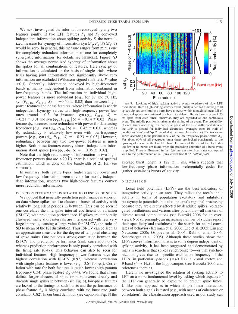
PREDICTION PERFORMANCE IS RELATED TO CLUSTERS OF SPIKES.

We noticed that generally prediction performance is superioron data where spikes tend to cluster to bursts of activity withrelatively long silent periods in between. This can be seen ifone correlates the interspike interval coefficient of variation(ISI-CV) with prediction performance. If spikes are temporallyclustered, many short intervals are interspersed with few verylarge intervals, causing a large value for ISI-CV, the ratio ofSD to mean of the ISI distribution. Thus ISI-CV can be seen asan approximate measure for the degree of temporal clusteringof spike trains. One notices a strong correlation between theISI-CV and prediction performance (rank correlation 0.86),whereas prediction performance is only poorly correlated withthe firing rate (0.47). This behavior can also be seen forindividual features. High-frequency power features have thehighest correlation with ISI-CV (0.92), whereas correlationwith single phase features is lower (e.g., 0.64 for �A). Corre-lation with rate for both features is much lower (high gammafrequency 0.34, phase feature �A 0.44). We found that if onedefines larger clusters of spike or burst events directly anddiscards single spikes in between (see Fig. 8), low-phase featuresare locked to the timings of such bursts and the performance ofphase feature �A is highly correlated with the burst rate (rankcorrelation 0.82). In our burst definition (see caption of Fig. 8) the

average burst length is 122 � 1 ms, which suggests thatlow-frequency phase information preferentially codes for(rather sustained) bursts of activity.

D I S C U S S I O N

Local field potentials (LFPs) are the best indicators ofintegrative activity in an area. They reflect the area’s inputactivity in terms of population excitatory and inhibitorypostsynaptic potentials, but also the area’s regional processingbecause they are directly affected by dendritic spikes, voltage-gated oscillations, and various after-potentials—all markers ofdiverse neural computations (see Buszaki 2006 for an over-view). Not surprisingly, an increasing number of studies reporttheir specificity and usefulness in the search for neural corre-lates of behavior (Kreiman et al. 2006; Lee et al. 2005; Liu andNewsome 2006; Osipova et al. 2006; Rubino et al. 2006;Scherberger et al. 2005). Although these studies show thatLFPs convey information that is to some degree independent ofspiking activity, it has been suggested and demonstrated bymany researchers that spikes synchronize to—or that synchro-nization gives rise to—specific oscillation frequency of theLFPs, in particular �-bands (�40 Hz) in visual cortex and�-band (4–8 Hz) in the hippocampus (see Buszaki 2006 andreferences therein).

Herein we investigated the relation of spiking activity toLFP on a more fundamental level by asking which aspects ofthe LFP can generally be exploited to predict spike times.Unlike other approaches in which simple linear interactionbetween both signals is tested (e.g., with means of coherence orcorrelation), the classification approach used in our study can

Pha

se o

f 1−

4Hz

[rad

]

0

2

4

6

Bur

st p

roba

bilit

y [%

]

0

1

2

3

4

5−101

20 40 60 80 100 1200

0.10.2

κ of

φA

Electrode no.

0

1

2

Burst rate [Hz]

FIG. 8. Locking of high spiking activity events to phases of slow LFPoscillations. Here a high spiking activity event (burst) is defined as having �10spikes. Spikes constituting a burst have to occur within a maximal mean ISI of5 ms, and spikes not contained in a burst are deleted. Bursts have to occur �25ms apart from each other; otherwise, they are regarded as one continuousevent. The middle position is taken as the timing of an event. The probabilityof event times occurring in a particular phase of the 1- to 4-Hz oscillation ofthe LFP is plotted for individual electrodes (averaged over 10 trials ofconditions “stm” and “spo” recorded at the same electrode site). Electrodes aresorted according to the performance of the low-frequency phase feature �A.For about 60% of all electrodes burst times are locked consistently to theupswing of a wave in the low LFP band. For most of the rest of the electrodestoo few or no bursts are found when the preceding definition of a burst eventis applied. Phase is illustrated in the right margin plot. Burst rates correspondwell to the performance of �A (rank correlation 0.82, bottom plot).




Dow

nloaded from


exploit multiple different features of the LFP simultaneously ina nonlinear way to infer spiking activity from LFPs. We foundthat when the best single feature is used, performance drops toabout 70%, showing that multiple features are essential. Thenonlinear component in the code is rather small, but there isstill an average increase of 12% when SVM classifiers areused.

In contrast to V1, the prediction of spikes from LFPs is(almost) impossible in the LGN. The reason for this could bethat spiking activity might be less correlated and thus have lesseffect on the LFP or, alternatively, that the geometrical ar-rangements of current sources and sinks in the thalamus gen-erate field potentials of lower spatial specificity than thoseobserved in cortex. Furthermore the fact that 80% of the LGNinput is cortical and modulatory is an additional potentialreason for the LFP-spiking decoupling in this nucleus. Neuro-modulation might explain our observation in simultaneousthalamus–cortex recordings that V1 LFP cannot predict LGNspiking. LGN–LFP, on the other hand, is a reasonable predictorof V1 spiking, likely because the former is a better indicator oflocal LGN activity that is correlated with the V1 LFPs, whichin turn can predict the spiking of this cortical area.

From the point of view that LFP is mostly generated by thetotality of synaptic input and local processing in a region onemight ask whether it is possible to predict spikes solely on thebasis of information preceding the actual time of the spike. Toevaluate this possibility we recomputed prediction perfor-mance for the same feature types but with shifted lags, so thatonly causal information of the LFP is included. When we didthis, prediction performance dropped to 68% of the averagenoncausal classifier used for the population analyses, which isstill well above chance level. However, conclusions about therelation between synaptic input and spiking output are difficultto draw from this number. For instance it is likely that due totemporal correlation in the spike train (and various LFP bands)neighboring times in the time series are good predictors foreach other.

LFP features related to spiking activity

Besides having generated and visualized concrete spiketrains inferred solely from information contained in the LFPs,our analysis revealed those features that are the most importantcarriers of information about spiking activity in the LFP andestimated their relative importance and redundancy properties.

The first and most useful feature for inferring spike trainsfrom LFPs is the power modulation of high-frequency compo-nents in the upper �-band from 40 to (at least) 90 Hz. This isin good agreement with other studies that have established alink between gamma-frequency bands and spiking activity(Csicsvari et al. 2003). The biophysical origin of gammafrequencies in the LFP remains a topic for current research.The rather fixed relationship between spikes and LFPs over awide range of data and conditions could reflect physical con-straints (layered organization of the cortex, distribution ofsinks, and sources) or inherent properties of the neural networktopology and function. For instance, gamma activity might bethe effect of fast inhibitory circuits on the LFPs (for a recentreview see Bartos et al. 2007).

In contrast to power modulations, phase in the �-range ismuch less important for prediction than one might have ex-

pected from the well-documented fact that spikes are synchro-nized in this range (Gray et al. 1989; Kreiter and Singer 1992).Our stimuli consist of cinema movies of several minutes’duration and containing a mixture of objects, faces, actions,colors, and edges. Thus specific object encoding might be weakand cluttered only with other aspects of the code because thestimulus consists of multiple objects at any given time. Be-cause we assume a stationary spike–LFP relation for theduration of a trial (170 s), more subtle aspects of the relationsuch as transient rapid neuron-to-neuron synchronizationswould be averaged out and therefore not detected as a usefulfeature. Another possibility for the relative unimportance ofgamma-phase features might be that different subgroups ofneurons present in the MUA signal lock to different phases inthe gamma cycle, as suggested for inhibitory and excitatoryneurons (Hasenstaub et al. 2005). In general, if two subgroupsof units present in the MUA signal locked to a different featureof the LFP, our classification method should not degrade inperformance because it can exploit many features simulta-neously. However, the relative usefulness of both featureswould indeed decrease in the average features analyses.

In addition, locking to phases of higher frequencies isdifficult to detect because even a small amount of jitter inspike-time precision abolishes locking. Such jitter might beintroduced during binning of the spike timings to LFP sam-pling resolution (5 ms). This is in contrast to the effect of asmall amount of jitter at lower frequencies. Accordingly, thephases of low-frequency components are indeed useful forpredicting spiking activity. Moreover, our analysis suggeststhat the oscillation phases of low frequencies code for largerbursts of temporally correlated spiking activity. In fact, thehigh probability of spikes occurring in clusters in our V1 datahelps to infer spikes from LFPs. Prediction quality is highlycorrelated with ISI-CV because one can predict spiking activityon a timescale of �25 ms, rather than reaching single spikeprecision. In the LGN data, where the spikes are less clustered(low ISI-CV, average of 1.1 � 0.05 compared with 2.4 � 0.05in anesthetized V1 and 1.8 � 0.05 in non-anesthetized V1), itis almost impossible to predict spikes from LFPs. Since weobserve stronger clustering for anesthetized data, we concludethat this might be partly an effect of anesthesia (Steriade et al.1993).

The low-frequency power modulations selected as usefulfeatures in a part of trials probably have origins similar to thoseof the slow-phase features and may code for the relativeamount and size of clusters of activity. Thus low-frequencypower modulations might provide a slow-changing state vari-able that is useful in combination with the fast-changinghigh-frequency powers, as indicated by the low redundancyvalues.

About half a century ago, several studies were conductedthat attempted to relate electrical encephalographic (EEG)signals to spiking activity. Then it was found that spikes occurpreferably at the negativity of 0.2- to 2-Hz waves (Fromm andBond 1964). Since EEG has a basis of origin similar to that ofLFPs (Nunez and Srinivasan 2006), this confirms our findings,where spikes occur at the minimum to rising phase of the slowoscillation. It is not just the negativity that is important,however, but also the peak that is seen following the spikes.This is similar to slow-wave sleep of cats as seen in the STA(Destexhe et al. 1999) and is taken to the extreme in spike-




Dow

nloaded from


wave complexes, which can be observed in cases of epilepsy(e.g., Destexhe et al. 2001). In the latter case, it was suggestedthat the slow positive wave form after a burst of activity isaccompanied by neuronal silence and can be explained by slowinhibitory effects mediated by �-aminobutyric acid type B(Destexhe et al. 2001). Although we observe neither clear up-and downstates nor any pathological periodic activity in theLFPs of our data, the similarity of the STA suggests that suchprocesses may play a role during more physiological states,albeit in a much weaker form.

Effects of spike detection method

The spiking signal used herein is generated by a simplethreshold-based procedure for detecting spiking events fromthe recordings. This detecting procedure is prone to false-positive detection, as well as to a smaller fraction of missedspikes originating at larger distances or from neighboringinterneurons. With our method we expect a false-positive rateof 2 Hz, if one assumes that nonspike values (i.e., noise) inMUA amplitudes are subject to Gaussian distribution (seeMETHODS). Thus the spiking signal contains not only the activityof multiple neurons and possibly of different cell types, butalso noise spikes. Since noise spikes should be independentlydistributed with respect to time, false-positive labels shouldactually reduce performance compared with the “true” spikingsignal. We tested higher spike detection thresholds, where thecontribution of noise becomes negligible (e.g., for 5SD only0.05 Hz), and found instead reduced prediction performance,although performance still remained well above chance (notshown). Since it was estimated that in principle spikes arisingfrom 1,000 neurons could be detected by a single electrode(Henze et al. 2000), a spiking signal generated with a higherthreshold will include fewer smaller spikes from neurons thatare further away and incorporate only those neurons thathappen to be in the immediate neighborhood of the electrodetip. Thus the spiking signal becomes more local and its rela-tionship to the relatively global LFP signal is naturally weaker.Therefore noise spikes are not likely to artificially enhance ourperformance results, but influencing the number of neuronswhose spikes are detected via threshold will have an effect.

Similarly, spike sorting yielding multiple single-unit activitiesrather than multiunit activity would naturally decrease predictionperformance, since spiking signals become more local and, addi-tionally, the prediction task would change from binary classifica-tion to a more difficult multilabel classification task.

Encoding of the stimulus

We found that the relationship between LFPs and spikes isalmost unchanged during stimulus-driven activity comparedwith spontaneous activity. This finding corresponds well to theresults of others (Fiser et al. 2004; Kenet et al. 2003; Vincentet al. 2007), who found that the structure of spontaneousactivity is rich and sometimes even resembles stimulus-drivenactivity. Although there is no general change in the structure offeatures, there are of course transient aspects of the stimuliencoded by spikes (and LFPs) that have an effect on the spikerate, for example, which increases during stimulus presentation(not shown). Because of the encoding of the changing moviestimulus over time, the temporally contiguous training and test

sets might differ in their LFP–spikes relation (i.e., in theirsample distributions). Thus movie encoding might explain whyprediction performance on spontaneous activity is slightlybetter than that on stimulus-driven activity.

Effects of stimulus encoding might also explain the obser-vation that the LFP is “more global” during spontaneousactivity in that prediction of spikes degrades much more slowlywith increasing cortical distance than that during stimuluspresentation. Thus the stimulus actually decorrelates neuralactivity spatially in comparison to spontaneous activity.

Note that we do not analyze features that actually encodeinformation about the stimuli. Information contained in LFPs andspiking activity about aspects of the movie stimulus will beinvestigated in a forthcoming paper (A Belitski, A Gretton, CMagri, Y Murayama, MA Montemurro, NK Logothetis, S Pan-zeri, unpublished observations) using the very same data as in thepresent study. Although we show here that the structure of therelationship of spikes and LFP does not change considerablyduring spontaneous activity, Belitski et al. nevertheless show thatvery low and very high oscillation powers of the LFP are highlyinformative about the stimulus. They find that high frequency LFPpower series (50–120 Hz) contain information about the stimulusthat is partially redundant with that in power series derived fromthe spike trains. In this respect, their results complement ours.

Conclusion

We conclude that to a certain degree spikes can be inferredfrom LFPs—a fact that reflects the interaction of these signals.However, we find that millisecond precision, which has beenshown to be used for temporal coding (Mainen and Sejnowski1995), cannot be inferred from LFP. The temporal aspects ofneural spiking used for information coding, rate coding, orcoding on spike timing remain a topic of current research(Rieke et al. 1999). We might conservatively say that irrespec-tive of whether they are important for coding, time-varyingrates on the scale of about a hundred milliseconds can bemoderately well inferred from the LFPs, but that exact timingscannot. Thus given our results, it should in principle bepossible to develop an appropriate methodology that permitsthe extraction of certain spiking features from signals measuredby methods relying on LFP-like signals, such as functionalMRI (Logothetis et al. 2001) or optical recordings (Grinvaldet al. 1985, 2004). Nevertheless, the strong dependence ofspike predictability on electrode position suggests that thereliability of such predictions may depend on the brain site.Finally, the fact that in the thalamus it is practically impossibleto predict spikes from the LFP suggests that computationsbased on input, local processing, and output—as instantiated inthe different frequency bands of the mEFP–can be helpful onlyfor structures with the appropriate element geometry (e.g.,fascicles of pyramidal cells vs. potentially close-field arrange-ment of thalamic neurons) and the proportion of driver tomodulator afferents.

A C K N O W L E D G M E N T S

We thank A. Tolias and G. Keliris for providing the non-anesthetized monkeydata set, A. Belitski for comments on earlier versions of the manuscript.

G R A N T S

This work was supported by the Max Planck Society and the AustrianScience Fund Project S9102.




Dow

nloaded from


R E F E R E N C E S

Ajmone-Marsan C. Electrical activity of the brain: slow waves and neuronalactivity. Israel J Med Sci 1: 104–117, 1965.

Arezzo J, Legatt A, Vaughan HGJ. Topography and intracranial sources ofsomatosensory evoked potentials in the monkey. I. Early components.Electroencephalogr Clin Neurophysiol 46: 155–172, 1979.

Bartos M, Vida I, Jonas P. Synaptic mechanisms of synchronized gammaoscillations in inhibitory interneuron networks. Nat Rev Neurosci 8: 45–56,2007.

Bishop CM. Pattern Recognition and Machine Learning. New York: Springer,2006.

Buchwald JS, Hala E, Schramm S. A comparison of multi-unit activity andEEG activity recorded from the same brain site in chronic cats duringbehavioral conditioning. Nature 205: 1012–1014, 1965.

Burges CJC. A tutorial on support vector machines for pattern recognition.Data Min Knowl Discov 2: 121–167, 1998.

Buzsaki G. Rhythms of the Brain. Oxford, UK: Oxford Univ. Press, 2006.Cohen J. A coefficient of agreement for nominal scales. Educ Psychol Meas

20: 37–46, 1960.Csicsvari J, Jamieson B, Wise KD, Buzsaki G. Mechanisms of gamma

oscillations in hippocampus of the behaving rat. Neuron 37: 311–322, 2003.Destexhe A, Contreras D, Steriade M. Spatiotemporal analysis of local field

potentials and unit discharges in cat cerebral cortex during natural wake andsleep states. J Neurosci 19: 4595–4608, 1999.

Destexhe A, Contreras D, Steriade M. LTS cells in cerebral cortex and theirrole in generating spike-and-wave oscillations. Neurocomputing 38: 555–563, 2001.

Fiser J, Chiu C, Weliky M. Small modulation of ongoing cortical dynamicsby sensory input during natural vision. Nature 431: 573–578, 2004.

Fromm GH, Bond HW. Slow changes in the electrocorticogram and theactivity of cortical neurons. Electroencephalogr Clin Neurophysiol 17:520–523, 1964.

Fromm GH, Bond HW. The relationship between neuron activity and corticalsteady potentials. Electroencephalogr Clin Neurophysiol 22: 159–166, 1967.

Gasser HS, Grundfest H. Axon diameters in relation to the spike dimensionsand the conduction velocity in mammalian A fibers. Am J Physiol 127:393–414, 1939.

Gray CM, Konig P, Engel AK, Singer. Oscillatory responses in cat visualcortex exhibit inter-columnar synchronization which reflects global stimulusproperties. Nature 338: 334–337, 1989.

Grinvald A. Real-time optical mapping of neuronal activity: from singlegrowth cones to the intact mammalian brain. Ann Rev Neurosci 8: 263–305,1985.

Grinvald A,Hildesheim R. VSDI: a new era in functional imaging of corticaldynamics. Nat Rev Neurosci 5: 874–885, 2004.

Grover FS, Buchwald JS. Correlation of cell size with amplitude of back-ground fast activity in specific brain nuclei. J Neurophysiol 33: 160–171,1970.

Hasenstaub A, Shu Y, Haider B, Kraushaar U, DuqueA McCormick DA.Inhibitory postsynaptic potentials carry synchronized frequency informationin active cortical networks. Neuron 47: 423–435, 2005.

Henze DA, Borhegyi Z, Csicsvari J, Mamiya A, Harris KD, Buzsaki G.Intracellular features predicted by extracellular recordings in the hippocam-pus in vivo. J Neurophysiol 84: 390–400, 2000.

Huang CM, Buchwald JS. Interpretation of the vertex short-latency acousticresponse: a study of single neurons in the brain stem. Brain Res 137:291–303, 1977.

Hunt C. The reflex activity of mammalian small-nerve fibers. J Physiol 115:456–469, 1951.

Jarvis MR, Mitra PP. Sampling properties of the spectrum and coherency ofsequences of action potentials. Neural Comput 13: 717–749, 2001.

Juergens E, Guettler A, Eckhorn R. Visual stimulation elicits locked andinduced gamma oscillations in monkey intracortical- and EEG-potentials,but not in human EEG. Exp Brain Res 129: 247–259, 1999.

Kamondi A, Acsady L, Wang XJ, Buzsaki G. Theta oscillations in somataand dendrites of hippocampal pyramidal cells in vivo: activity-dependentphase-precession of action potentials. Hippocampus 8: 244–261, 1998.

Kenet T, Bibitchkov D, Tsodyks M, Grinvald A, Arieli A. Spontaneouslyemerging cortical representations of visual attributes. Nature 425: 954–956,2003.

Kreiman G, Hung CP, Kraskov A, Quiroga RQ, Poggio T, DiCarlo JJ.Object selectivity of local field potentials and spikes in the macaque inferiortemporal cortex. Neuron 49: 433–445, 2006.

Kreiter AK, Singer W. Oscillatory neuronal responses in the visual cortex ofthe awake macaque monkey. Eur J Neurosci 4: 369–375, 1992.

Lee H, Simpson GV, Logothetis NK, Rainer G. Phase locking of singleneuron activity to theta oscillations during working memory in monkeyextrastriate visual cortex. Neuron 45: 147–156, 2005.

Liu J, Newsome WT. Local field potential in cortical area MT: stimulustuning and behavioral correlations. J Neurosci 26: 7779–7790, 2006.

Logothetis N, Merkle H, Augath M, Trinath T, Ugurbil K. Ultra high-resolution fMRI in monkeys with implanted RF coils. Neuron 35: 227–242,2002.

Logothetis NK. The underpinnings of the BOLD functional magnetic reso-nance imaging signal. J Neurosci 23: 3963–3971, 2003.

Logothetis NK, Pauls J, Augath M, Trinath T, Oeltermann A. Neurophys-iological investigation of the basis of the fMRI signal. Nature 412: 150–157,2001.

Mainen ZF, Sejnowski TJ. Reliability of spike timing in neocortical neurons.Science 268: 1503–1506, 1995.

Mitzdorf U. Current source-density method and application in cat cerebralcortex: investigation of evoked potentials and EEG phenomena. Physiol Rev65: 37–99, 1985.

Mitzdorf U. Properties of the evoked potential generators: current source-density analysis of visually evoked potentials in the cat cortex. Int J Neu-rosci 33: 33–59, 1987.

Musicant DR, Kumar V, Ozgur A. Optimizing f-measure with support vectormachines. In: Proceedings of the Sixteenth International Florida ArtificialIntelligence Research Society Conference, edited by Russell I, Haller S.Cambridge, MA: AAAI Press/MIT Press, 2003, p. 356–360.

Nadasdy Z, Csicsvari J, Penttonen M, Hetke J, Wise K, Buzsaki G.Extracellular recording and analysis of neuronal activity: from single cells toensembles. In: Neuronal Ensembles: Strategies from Recording and Decod-ing, edited by Eichenbaum HB, Davis JL. New York: Wiley–Liss, 1998, p.17–55.

Natschlager T, Maass W. Dynamics of information and emergent computa-tion in generic neural microcircuit models. Neural Networks 18: 1301–1308,2005.

Nelson PG. Interaction between spinal motoneurons of the cat. J Neurophysiol29: 275–287, 1966.

Nunez PL, Srinivasan R. Electric Fields of the Brain: The Neurophysics ofEEG (2nd rev. ed.). Oxford, UK: Oxford Univ. Press, 2006.

Osipova D, Takashima A, Oostenveld R, Fernandez G, Maris E, Jensen O.Theta and gamma oscillations predict encoding and retrieval of declarativememory. J Neurosci 26: 7523–7531, 2006.

Panzeri S, Senatore R, Montemurro MA, Petersen RS. Correcting for thesampling bias problem in spike train information measures. J Neurophysiol98: 1064–1072, 2007.

Percival DB, Walden AT. Spectral Analyses for Physical Applications.Cambridge, UK: Cambridge Univ. Press, 2002.

Pola G, Thiele A, Hoffman K-P, Panzeri S. An exact method to quantify theinformation transmitted by different mechanisms of correlational coding.Network Comput Neural Syst 14: 35–60, 2003.

Rieke F, Warland D, de Ruyter van Steveninck R, Bialek W. Spikes:Exploring the Neural Code. Cambridge, MA: MIT Press, 1999.

Rubino D, Robbins KA, Hatsopoulos NG. Propagating waves mediateinformation transfer in the motor cortex. Nat Neurosci 9: 1549–1557, 2006.

Scherberger H, Jarvis MR, Andersen RA. Cortical local field potentialencodes movement intentions in the posterior parietal cortex. Neuron 46:347–354, 2005.

Schneidman E, Bialek W, Berry MJ. Synergy, redundancy, and indepen-dence in population codes. J Neurosci 23: 11539–11553, 2003.

Scholkopf B, Smola AJ. Learning with Kernels. Cambridge, MA: MIT Press,2002.

Steriade M, McCormick DA, Sejnowski TJ. Thalamocortical oscillations inthe sleeping and aroused brain. Science 262: 679–685, 1993.

Thomson DJ. Spectrum estimation and harmonic analysis. Proc IEEE 70:1055–1096, 1982.

Tolias AS, Ecker AS, Siapas AG, Hoenselaar A, Keliris GA, LogothetisNK. Recording chronically from the same neurons in awake, behavingprimates. J Neurophysiol 98: 3780–3790, 2007.

Vapnik VN. The Nature of Statistical Learning Theory. Berlin: Springer-Verlag, 1999.

Vincent JL, Patel GH, Fox MD, Snyder AZ, Baker JT, Van Essen DC,Zempel JM, Snyder LH, Corbetta M, Raichle ME. Intrinsic functionalarchitecture in the anaesthetized monkey brain. Nature 447: 83–86, 2007.




Dow

nloaded from


malte j. rasch, arthur gretton, yusuke murayama, wolfgang...

Documents