Tech

nica

l Whi

te P

aper

QCL-TWP-Maintenance-For-Online-AnalysersOctober 2015

Maintenance Strategies for Online Analysers

Introduction

Calibrate, calibrate!

Wouldn’t it be wonderful if after commissioning, an online analyser started up already in perfect calibration? If during its life it was able to check that it remained in calibration without the need for test samples? If it could work for very long periods without the need for maintenance intervention, but when eventually some intervention was required, the analyser would raise a flag along with a description of why maintenance was needed? Would this be desirable? Of course! But is it feasible?

This paper is a thought piece: it is intended to initiate a discussion about the development of maintenance practices for online analyser over recent years. It considers what factors mean that calibrations and validation checks must be carried out and how maintenance schedules are planned. Then it looks at the information content that is available with some modern analyser technologies and asks if there is a way of utilising that information to greatly minimise, perhaps even eliminate, planned preventative maintenance, validation checks and calibrations.

Many organizational issues as well as technical problems need to be solved before maintenance-free analysers become a reality, but sound science and good mathematics indicate that perhaps it is time to give serious consideration to how this lofty goal might be approached.

What major developments have there been in the maintenance strategies for online analysers over the last few decades? Up until the early 1980s, the approach most frequently adopted was that on a periodic basis a standard sample was introduced to an analyser and its output was adjusted to match the value of that standard: the analyser was recalibrated each time it was checked. Facilities for the introduction of standard samples were invariably included as part of the design of the samples system (1).

This strategy had several things in its favour. It was easy to implement and was conceptually simple. A calendar based scheduler told technicians when to do the task. The standard sample was introduced and after making the adjustment there was no doubt that the analyser was in perfect calibration.

2

The only record keeping required was to note the date on which the calibration was carried out.

Occasionally a data user might question the results from an analyser between scheduled maintenance trips and the simplicity of going out and recalibrating on demand was satisfactory all round. Everyone knew that the analyser was in calibration after the maintenance visit and the day’s work could carry on.

This simple approach went a long way. The only thing to decide was how frequently a calibration should take place and that decision was essentially heuristic, based on the complexity of the analyser and a feel for how critical an error in calibration would be. For something simple, like a pH analyser, the calibration interval might be 3 months; for something more complex, like a PGC, it might be once a week.

Validate, validate!

In the 1980s the Quality Movement (with a capital Q and a capital M!) challenged the Calibrate, Calibrate methodology by the application of statistics. The origins of the new approach were in the mid-1920s when Walter Shewart, a physicist at Bell Laboratories, designed the Statistical Quality Control (SQC) method for zero defects in mass production. On 16 May, 1924 Shewart issued a memorandum that contained a sketch of a control chart and in 1931 he published his book “Economic Control of Quality of Manufactured Product” (2), in which he provided a precise and measurable definition of quality control and described statistical techniques for evaluating production and improving quality. During World War II, W. Edward Deming (3) and Joseph Juran (4) separately advanced Shewart’s work and developed the versions of SQC which became commonly used in the 1980s. Although it is widely accepted that the Japanese owed their product leadership in part to adopting the precepts of Deming and Juran, 40 years passed before US industry converted to SQC.

Online analyser maintenance strategies embraced SQC. Instead of recalibrating each time a standard sample was introduced, the new approach was to recalibrate only if there was evidence of a systematic failure somewhere in the system, and even then recalibration should only take place after that failure had been identified and fixed.

To set up an SQC programme, after commissioning, the performance of an analyser was quantified. In particular, the random variations found in the measurement results of an analyser which was working correctly were determined. Thereafter, a standard sample (now known as a benchmark sample) would be introduced periodically and the result would be assessed for whether or not it was within the normal variation of the analyser; this would typically be done using an SQC chart in combination with the application of a set of rules (5). If the analyser result was inside the usual variation then no further action would be taken: the analyser was considered to be “in control” and it wasn’t recalibrated. If it failed the test, then the reason for failure had to be investigated and until it was identified and cured there would be no point in recalibrating the analyser or returning it to service since it was clear that there was something wrong somewhere in the analyser system.

The SQC approach was more complex than Calibrate, Calibrate. It was still driven by a scheduler but now, after the introduction of the standard sample it was necessary to manipulate the result, plot it on a chart and apply a set of rules to see if the analyser passed the test or not. The record keeping required storing more data as well as keeping control charts, and there was the additional complexity of having to adjust the charts whenever a standard blend ran out and a new one was brought in. To use the system properly, technicians had to be familiar with the statistical basis of SQC, which meant more training. In addition, if a data user asked for a recalibration because the analyser measurements didn’t look right, now the response would not be a calibration at all – instead there would be a benchmark test and it might be that although the result didn’t exactly match the standard, there would be no correction. To accept this, the data user also had to understand the statistical basis of the programme.

3

Despite these obstacles, SQC offered several powerful advantages which made the extra complexity well worthwhile:

� Quantified performance. During the set-up period, a record of benchmark tests meant that the variation of each individual analyser was quantified. The analyser’s spec sheet might give an accuracy of, say, ±2 % of reading, but the set-up tests allowed the actual variation to be estimated; often it was lower than the spec sheet limits. Knowledge of error is important for process control, particularly if measurement data are being used to make a plant operate just inside a specification limit.

� Reduced variation or noise in readings. Suppose the actual variation of an analyser is ±1.5 % of reading. It turns out that by recalibrating an analyser each time it is checked, the statistical variation is compounded and over time the analyser delivers a variation of √2 x 1.5 = 2.1 % of reading: although it actually had better performance than the spec sheet claimed, the Calibrate, Calibrate approach leaves it delivering poorer performance.

� Failures identified and fixed. There should be no fear in using tighter limits than those on the spec sheet to decide if an analyser is working properly: the set-up period has already established that the analyser can indeed meet those limits. But then during ongoing operation, individual benchmark results which are outside the normal variation, or a sequence of results which show a trend in one direction (the run rule test) make it clear that something is failing somewhere in the system. Simply recalibrating would mask such failures and significant measurement errors could build up before the next scheduled calibration test. With SQC it is clear that something has changed and there is now a quantifiable way to tell whether maintenance has been effective in fixing it.

� Fewer process control bumps. Analyser data are frequently used in closed loop process control applications with the objective of making a plant operate in as stable a way as possible at the economically optimum position. However, analyser recalibration causes a step change in the analyser data with a consequent step change in process control settings to compensate. It is often the case that in a sequence of process units, a small shift in the operation of a unit at the start of the chain is amplified in size as process fluids pass along the chain. This ripple effect can lead to a significant deviation from the economically optimum operating position and it can take many minutes before the process control applications are able to restore stable operation: these ripples cause a costly, but often unrecognised, operating cost.

� Cheaper test blends. Calibration blends need to be traceable to a standard and are consequently costly to produce: it’s necessary to pay for accuracy. A benchmark blend on the other hand need not be accurately characterised, and in fact a sample from the process stream could be used. All that is required is that its composition remains stable over a long period of time. Relatively inexpensive benchmark blends can be used for validation checks, reserving the more expensive calibration blends only for occasions when recalibration really is necessary.

� Life history. An SQC programme records all work carried out on an analyser, often with notes or comments added to control charts. Over time the performance and problems of each individual analyser are documented. Such a history for each analyser allows data-based optimisation of its maintenance programme. In addition, looking amongst a group of similar analysers it is possible to identify bad actors and put continuous improvement programmes in place. There is also a way to quantify the effectiveness of such improvement programmes.

The net effect of these advantages are lower total costs and an improved cost benefit ratio for analysers and for these reasons analyser SQC programmes became the industry norm.

4

Prevaricate, prevaricate!

Calibration and Validation

SQC seemed like the end point for analyser maintenance strategies, but then in the 2000s another concept came along: risk based maintenance (RBM). This defined the overall objective of the maintenance process as increasing profitability and optimizing the total life cycle cost without compromising performance (6).

Risk assessment was a decision tool for preventive maintenance planning and it aimed to minimise the probability of system failure, leading to better asset and capital utilization. The elements of RBM were risk estimation, followed by risk evaluation which then led to maintenance planning.

Risk estimation meant figuring out how likely it would be that a failure would occur, especially paying attention to the likelihood of unrevealed failures. Then the cost of such a failure would be estimated. Using these two factors it was possible to design a maintenance programme which balanced the cost of maintenance activities against the potential cost of failures: maintenance work, including validation checks, would be put off unless they made overall economic sense. (The heading for this section is a tongue in cheek view of how some people in the analyser world regard RBM: it has not yet received full acceptance in all quarters and is sometimes viewed as merely putting off what will have to be done anyway).

The formal definition of calibration which is given by the International Bureau of Weights and Measures is (7):

"Operation that, under specified conditions, in a first step, establishes a relation between the quantity values with measurement uncertainties provided by measurement standards and corresponding indications with associated measurement uncertainties (of the calibrated instrument or secondary standard) and, in a second step, uses this information to establish a relation for obtaining a measurement result from an indication.”

Behind this definition is the requirement that there are physical laws (laws of science) which govern the relationship between the indications and the quantity which is to be measured. Consider, for example, the Beer Lambert Law (8), (9), which is the basis for photometric or spectroscopic measurements:

I --- = exp(-εcl) (1) Io

where Io = intensity of incident radiation I = intensity of transmitted radiation ε = absorbtivity of an attenuator at the wavelength of the radiation c = concentration of an attenuator l = distance that radiation travels through the attenuator (the path length).

Consequently, the concentration of the attenuator is given by:

- ln (I / Io)c = -------------- (2) ε l

5

Non-dispersive Infrared (NDIR) Photometers

Revealed and Unrevealed Errors

If the natural logarithm of the ratio of the transmitted to incident radiation is found (these are the indications), then the process of calibration is effectively the process of finding a constant of proportionality to account for -1 / ε l.

c = K ln (I / Io) (3)

where K is the calibration constant.

Since K is related to ε and l and they are both constants, any subsequent validation is a check that nothing has had an impact on the measurement of ln (I / Io).

It is worth noting at this point that in principle, if the analyser is designed so that ln (I / Io) can be determined directly, then since the path length, l, can be measured and the absorbtivity, ε, could be looked up, there would not be a need to determine the calibration constant K experimentally: it could be calculated. The calibration would in effect be made from first principles.

Measurement of the individual, absolute intensities of Io and I would be a difficult challenge. However, since it is the ratio of the two light intensities that is required, smart design of the analyser can allow that ratio to be measured directly.

For an NDIR photometer relying on the Beer lambert law, what effects could compromise the measurement of ln (I / Io)?

To answer this question it is necessary to look in more detail at the design of NDIR analysers. For a specific measurement application, a wavelength of light is selected which is strongly absorbed by the substance which is to be measured (this is the attenuator in the discussion above) but is not absorbed by any other species in the sample. A large absorption means that the substance has a high value of the absorbtivity, ε, at that wavelength. An interference filter is used which allows light of that wavelength, known as the measurement wavelength, to pass into a cell which contains the sample. The path length of the cell is l in equations (1) and (2) and the intensity of the light coming out of the cell and falling on the detector is I. The intensity of light going into the cell is estimated by using another interference filter at a wavelength which is close to the measurement wavelength, but which is not absorbed by any species in the sample: this is called the reference wavelength. If the two filters are mounted on a wheel which spins round alternately putting the measurement then reference wavelengths into the light path, the signal strengths at the detector for each wavelength are (close to being) proportional to I and Io. The ratio of I to Io is easily found, from this the natural logarithm can be derived and in combination with the calibration constant, K, the concentration, c, of the component of interest can be found.

For an NDIR photometer relying on the Beer lambert law, are there effects could cause errors in the measurement of ln (I / Io)?

One way that this could be disturbed would be if the intensity of the incident radiation, Io, were severely attenuated. A lower intensity of light would lead to a poorer signal to noise ratio. It could also affect the fidelity with which the reference wavelength represented the intensity of the incident light. Such an effect could be caused by a change in the light source itself, for example aging; sources nearing the end of their life exhibit a drop in intensity. However, if the intensity of the reference wavelength is monitored during normal operation, it is possible to tell if such an effect has taken place. A low light alarm could be raised when the intensity of the reference wavelength drops below a set value and hence this type of error is referred to as a revealed error. Consequently, there is no need to use a validation test to detect such an error since it can be readily discovered by the analyser itself when running on a process sample.

6

Another way that the reliability of the measurement of ln (I / Io) could be compromised could be by a build-up of material on the windows of the cell, scattering or absorbing light at the measurement wavelength but not the reference wavelength. There is not a way to detect this in normal operation since the attenuation of the measurement wavelength could equally well have been due to absorption by the component being measured. Such an effect is called an unrevealed error. It would be discovered by a validation test: the additional attenuation of the measurement wavelength would manifest itself as an apparent increase in the concentration of the measured component in the standard and this would show up on a process control chart.

A third way in which the measurement could be compromised would be if an additional component was present in the sample, perhaps due to a new process operating regime. If this component absorbs light at either the measurement or reference wavelength, then clearly the measurement will be affected. Once again, in normal operation such an effect would be an unrevealed failure. A validation test in which the sample cell is flushed with a standard sample would also fail to detect this error since the interfering component would no longer be present in the cell.

In summary, if errors can be detected during the normal operation of an analyser on a process sample, then they are called revealed errors and as long as the method of detecting them is robust, then there is no need to discover them by a validation test. Only unrevealed errors, which are not apparent in normal operation, require a validation test for their detection. However, there can be errors which are not revealed by validation tests.

The Process Gas Chromatograph (PGC)

The PGC is the work-horse online analyser. It gives multicomponent measurements with a wide dynamic range of a large number of analytes. Measurement by a PGC could be comprised of the following sequence (not every PGC application uses all of these steps):

� Injection of a volume of sample.

� Use of a splitter to adjust the quantity of sample to give compatibility with the sensitivity of a detector.

� Separation of components by one or more chromatographic columns. This could include manipulations such as foreflush, backflush or heart-cut techniques.

� Detection by TCD, FID or other technique.

� Peak picking and peak integration.

� Conversion to real world measurement units

It is clear why calibration is essential and periodic validation is required for PGCs. The path from injection of a certain number of molecules to detection of those molecules as they pass through the detector is tenuous. Each stage, of course, has associated physical laws which describe it but trying to calculate a calibration from first principles would be a tough challenge indeed.

By injecting a known volume of sample at a particular pressure, the gas laws could be used to estimate the number of molecules injected. Measuring the ratio of flows at the splitter would allow the dilution of the sample to be calculated. If foreflush and backflush are perfectly set up, then no molecules would be unexpectedly lost in those operations. If columns were perfect then there could be complete separation of all components. If the efficiency of the detector were known then the number of molecules passing by could be estimated. And if peak picking and integration worked perfectly, then the amount of each component could be calculated from first principles. However, there are just too many steps in that process to make a calibration based on fundamental first principles practical; it’s much easier to calibrate using a standard blend.

7

Similarly, at each stage in the measurement process there are effects which could lead to unrevealed errors. A build up of material in the injection valve could affect the volume; flows at the splitter could drift, altering the dilution; changes in column efficiency could affect peak separations; elution time drifts could lead to molecules being lost during foreflush or backflush; detector efficiency could degrade; peak picking software could swap between algorithms due to small changes in peak characteristics. Clearly with so many potential unrevealed errors, validation must be an important part of the maintenance strategy for PGCs. The fact that nowadays many PGC applications can run in reliable calibration for several months is a great tribute to the ingenuity and skills of PGC designers who have systematically worked through and mitigated potential sources of error. The fact remains though, that PGCs require both calibration and periodic validation.

Tuneable Laser Spectroscopy

The Information Content of Some Modern Analysers

The preceding discussion has highlighted that if an analyser has internal methods of identifying errors, then these are called revealed errors and as long as the analyser has a way to report such errors, there is no need to discover them by validation tests. Validation tests are required to identify and correct unrevealed errors; however, some types of unrevealed error might not be detected by validation tests. The possibility was raised that under some circumstances it might be feasible to calibrate an analyser from first principles, not by using a calibration standard.

At this point, consider whether the information content of some types of analyser could open the door to extremely long periods of operation without the need for validation checks. And more controversially, are there any circumstances under which calibrations could be dispensed with too?

Quantum Cascade Laser (QCL) spectrometers have a high information continent. A QCL works in the mid-IR: the fingerprint region of the spectrum where absorption peaks are narrow and intense. QCLs scan over several wavenumbers and record an absorption spectrum which typically includes several features in addition to the absorption peak of the component to be measured. Can the processing of this complete set of information eliminate unrevealed errors and hence remove the need for validation tests?

Signal Processing in QCL Spectrometers

In a QCL spectrometer operating in pulsed mode, the laser is fired at a pulse repetition frequency of, typically, 50 kHz and the duration of each pulse is of the order of 500 ns. During a pulse the wavelength of the emitted light scans over about 1–5 wavenumbers. The laser light passes through a cell containing the sample to be measured and then goes to a detector. The raw signal from the detector is digitised and passed forward for signal processing.

A large number of individual pulses are accumulated to give a good signal to noise ratio and Figure 1 shows an unprocessed detector signal for a sample which contains carbon monoxide (CO) and ethylene. The x-axis is in units of time and the y-axis is the detector in signal volts.

8

Figure 1 - Raw Detector Signal for a Mixture of CO and Ethylene

Figure 2 - The Spectra of CO and Ethylene in the Fit Region

Next the time axis is converted into a wavenumber axis. An etalon can be inserted into the light path to give precise wavelength intervals and a known absorption peak in the scan can be used as a reference point for the wavelength scale. The final stage of signal processing is to set the start and finish points of the spectrum – a fit window which includes the features required to generate concentrations. This is the measured spectrum.

These initial adjustments are followed by a sophisticated fitting process which differs fundamentally from the data manipulation carried out in conventional photometers or spectrometers. The details of the process are proprietary but in general terms processing proceeds as follows.

Gas databases are generated for each component which could be present in the sample. A gas database is a collection of physical parameters that describe the response of individual absorption lines to temperature, pressure, concentration, presence of other gases, etc. They can be considered to be physical constants that can be used to simulate absorption spectra. Figure 2 shows the spectra of CO and ethylene from which gas databases are generated.

9

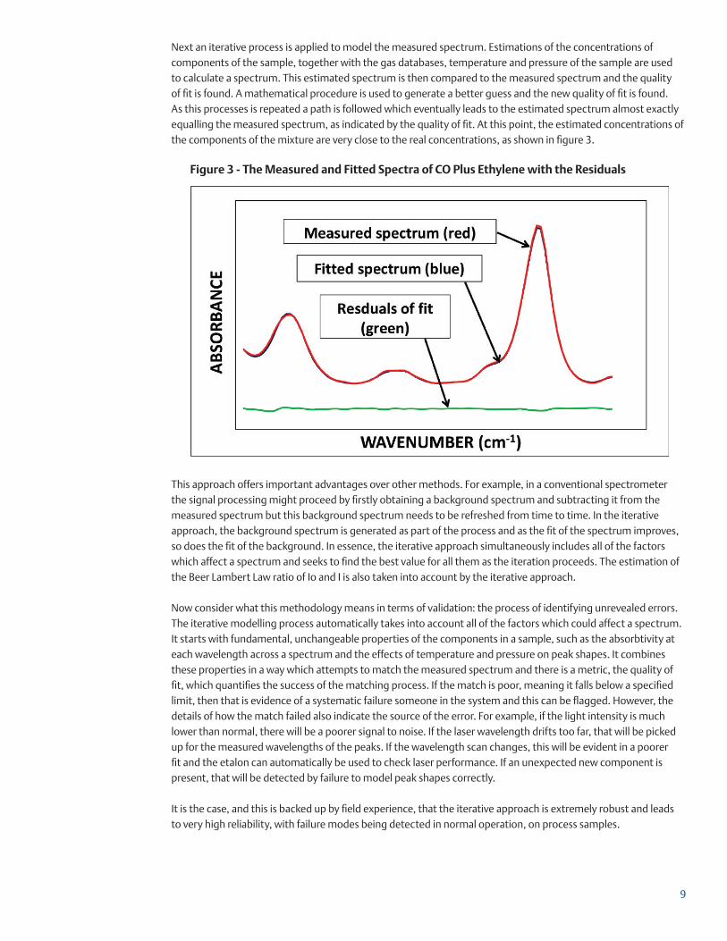
Figure 3 - The Measured and Fitted Spectra of CO Plus Ethylene with the Residuals

Next an iterative process is applied to model the measured spectrum. Estimations of the concentrations of components of the sample, together with the gas databases, temperature and pressure of the sample are used to calculate a spectrum. This estimated spectrum is then compared to the measured spectrum and the quality of fit is found. A mathematical procedure is used to generate a better guess and the new quality of fit is found. As this processes is repeated a path is followed which eventually leads to the estimated spectrum almost exactly equalling the measured spectrum, as indicated by the quality of fit. At this point, the estimated concentrations of the components of the mixture are very close to the real concentrations, as shown in figure 3.

This approach offers important advantages over other methods. For example, in a conventional spectrometer the signal processing might proceed by firstly obtaining a background spectrum and subtracting it from the measured spectrum but this background spectrum needs to be refreshed from time to time. In the iterative approach, the background spectrum is generated as part of the process and as the fit of the spectrum improves, so does the fit of the background. In essence, the iterative approach simultaneously includes all of the factors which affect a spectrum and seeks to find the best value for all them as the iteration proceeds. The estimation of the Beer Lambert Law ratio of Io and I is also taken into account by the iterative approach.

Now consider what this methodology means in terms of validation: the process of identifying unrevealed errors. The iterative modelling process automatically takes into account all of the factors which could affect a spectrum. It starts with fundamental, unchangeable properties of the components in a sample, such as the absorbtivity at each wavelength across a spectrum and the effects of temperature and pressure on peak shapes. It combines these properties in a way which attempts to match the measured spectrum and there is a metric, the quality of fit, which quantifies the success of the matching process. If the match is poor, meaning it falls below a specified limit, then that is evidence of a systematic failure someone in the system and this can be flagged. However, the details of how the match failed also indicate the source of the error. For example, if the light intensity is much lower than normal, there will be a poorer signal to noise. If the laser wavelength drifts too far, that will be picked up for the measured wavelengths of the peaks. If the wavelength scan changes, this will be evident in a poorer fit and the etalon can automatically be used to check laser performance. If an unexpected new component is present, that will be detected by failure to model peak shapes correctly.

It is the case, and this is backed up by field experience, that the iterative approach is extremely robust and leads to very high reliability, with failure modes being detected in normal operation, on process samples.

Calibration

10

It has been shown that if sufficient information is available, and if it can be effectively manipulated, then unrevealed errors can be eliminated, hence removing the need for validation tests. This is an economically attractive proposition. However, the elimination of unrevealed errors implies that the calibration must, therefore, also be sound. Again, there is field evidence that this is the case: long periods of reliable operation without calibration drift have been achieved.

It has also been suggested that there are circumstances in which a calibration could be made from first principles. But in reality, in today’s world of Process Analytics, is that a desirable objective? Since QCL systems will in any case continue to be designed with a means of introducing validation or calibration samples, what would be the point of calibrating from first principles?

A first principle calibration would be desirable when it is extremely difficult or extremely expensive to produce a calibration standard. Examples of this are low concentration blends of unstable mixtures, such as low- or sub-ppm blends of moisture, ammonia or sulphur compounds. These materials are readily absorbed and desorbed from the surfaces of gas cylinders, the tubing of sample systems and the walls of sample cells. Techniques such as passivation of the surfaces of contacted materials are used minimise such effects but on switching in a low ppm standard, it can take a very long time for stability to be achieved. The amount of material absorbed is temperature dependant and so there is also sensitivity to temperature change in the system. Often such standards have to be made using an inert bulk gas, such as nitrogen, instead of the gases representing the process stream. Frequently the cylinder pressure has to be low to prevent high vapour pressure components from condensing out of the blend.

The difficulty of producing stable cylinders of standards has led to other techniques being tried. Calibrated leaks into a carrier stream, various types of diffusion device, or the careful dilution of higher concentration blends have all been employed.

However the net effect of using standard blends for these hard-to-work with components is that often when a validation test is failed it is not clear whether that is due to the analyser or the blend being out of control. In addition, there is a comparatively high level of uncertainty (or noise) in the accuracy of the standard, also affecting confidence in the of the fidelity of calibrations.

Under these circumstance at least, it seems that there is a worthwhile incentive to examine whether an approach based on calibration from first principles could work. In general, a work programme might have two elements:

� Development of the science and mathematical manipulations required to give a first principles calibration.

� Careful development of a method to prepare a calibration blend in order to verify the first principles calibration.

Following the success of those two steps, future calibrations would rely on the first principles approach. The interesting question then arises: if this is works for hard-to-use components, why wouldn’t it work to for other components too?

In addition to raising alarms when a failure is present, there is an additional powerful advantage of this approach. If the quality of fit is high, that is strong evidence that the analyser is functioning correctly. This is a step out from the usual situation. Having positive evidence, obtained in real time on process samples, that an analyser is operating correctly is a significant step forward in analyser validation and credibility.

11

Conclusion

There is no doubt that the tried and trusted approach of analyser validation based on SQC will continue to be used. Equally, analyser calibration using standard blends will also remain in place. The intention of this paper was not to cast doubt on the efficacy of these methodologies. However, maintenance strategies have evolved over time, from when regular recalibration was the norm, through to the implementation of SQC-based validation tests and more recently the inclusion of risk based approaches to determine the frequency of maintenance interventions. The drivers for this evolution have been the desire to improve analyser performance and to reduce the cost of ownership.

The key to setting the frequency of validation test is in understanding unrevealed failures. Most of today’s analysers have checks built in which will identify some failures in the system. When these checks are comprehensive and reliable, the chance of unrevealed failures is reduced and the validation frequency can be increased. Validation is only needed to detect unrevealed failures – but there are some failure modes which will not be identified even by validation tests.

In some modern analysers, such as QCL spectrometers, there are more sophisticated ways of detecting failures using the high information content inherent in the measurement, hence the chance unrevealed errors is greatly reduced. This paper introduces the concept that by utilising the information available in QCL spectrometers, it is possible to go further still: in addition to affirming that there is no evidence of failure, it is also possible to state that there is positive evidence that an analyser is working correctly, based on data gathered in real time on process samples. This can lead to very long intervals between the need for validation tests and perhaps, based on the evidence of many QCL spectrometers operating in the field, to the elimination of routine validation tests. Instead maintenance interventions will be driven by the analyser itself identifying failures using information gathered in real time on process samples.

The approach of calibrating analysers by using standard blends is straight forward and intuitively correct. However, for some difficult-to-work-with materials, this approach is extremely difficult or extremely expensive to implement. This paper raises the possibility that instead, a reliable calibration might be achieved from a first principles approach provided that it the methodology could be initially validated using a calibration standard. If that were indeed proved possible, then the intriguing question arises of why could the same approach not be applied to any sample? Once again, before this could ever become a normal practice, considerable evidence based on field experience with many analysers would be required.

The intention of this paper is initiate a discussion, based on sound science and economic imperatives, about whether extreme extension of validation periods is possible and whether there are a ways in which calibrations could be eliminated. Regard it as a thought piece. Where are the gaps in the logic? What barriers, both technical and organisational, would have to be overcome in order to make progress on these ideas? Can some of the principles outlined here be applied to other types of analyser? Above all, think about what could be done to improve the performance and decrease the costs of using online process analysers by taking a fresh look at ways of utilising the full information content available in online analysers.

References1. McLennan, F. and Kowalski, Bruce R., “Sampling Systems”, Process Analytical Chemistry, Blackie Academic

and Professional, 1995, Page 37.

2. Shewhart, Walter A., Economic control of quality of manufactured product. D. Van Nostrand Company, New York, 1931.

3. Deming, W. Edwards, Statistical Adjustment of Data John Wiley and Sons, Dover, 1943

4. Juran, Joseph, Quality Control Handbook, McGraw-Hill, New York, 1951

5. Wheeler, Donald J., and David S. Chambers, Understanding Statistical Process Control, 3rd Edition, SPC Press, Knoxville, Tennessee, 2010

6. Khan, Faisal I and Haddara Mahmoud M, “Risk-based maintenance (RBM): a quantitative approach for maintenance/inspection scheduling and planning”, Journal of Loss Prevention in the Process Industries, Volume 16, Issue 6, November 2003, Pages 561–573.

7. Bureau International des Poids et Mesures, “Evolving Needs for Metrology in Material Property Measurements”, CIPM09 Materials WG Report Part 2, 2007 http://www.bipm.org/cc/CIPM/Allowed/96/CIPM09_Materials_WG_Report_Part_2.pdf

8. J.H. Lambert, “Photometria sive de mensura et gradibus luminis, colorum et umbrae” [Photometry or On the measure and gradations of light, colours, and shade] Augusta Vindelicorum, Eberhardt Klett, Augsburg, Germany:, 1760, Page 391.

9. A. Beer (1852) "Bestimmung der Absorption des rothen Lichts in farbigen Flüssigkeiten" (Determination of

the absorption of red light in colored liquids), Annalen der Physik und Chemie, vol. 86, pp. 78–88.

©2015 Emerson Process Management. All rights reserved.

The Emerson logo is a trademark and service mark of Emerson Electric Co. All other marks are the property of their respective owners.

The contents of this publication are presented for information purposes only, and while effort has been made to ensure their accuracy, they are not to be construed as warranties or guarantees, express or implied, regarding the products or services described herein or their use or applicability. All sales are governed by our terms and conditions, which are available on request We reserve the right to modify or improve the designs or specifications of our products at any time without notice.

EmersonProcess.com/GasAnalysis

Analyticexpert.com

Twitter.com/Rosemount_News Facebook.com/Rosemount

YouTube.com/user/RosemountAnalytical

Emerson Process Management Cascade TechnologiesGlendevon HouseCastle Business ParkStirling, FK9 4TZScotlandT + 44 1786 447 721F + 44 1786 475 822QCL.CSC@Emerson.com