Tectonoph~srcs. 105 (1984) 355-371

Elsevier Science Publishers B.V.. Amsterdam - Printed in The Netherlands

355

MAGNETOMETER ARRAY STUDIES IN INDIA AND THE LITHOSPHERE

B.J. SRIVASTAVA ‘, B.P. SINGH 2 and F.E.M. LILLEY ’

’ Nurronal Geophystcui Research lnstrtute, Hydemhad-500007 (Indru)

’ Indran Institute of Geomagnetism, Bombay - 400005 (Indru)

.’ Reseurch School of Earth Sciences, Austruhan Nuttonul Unroersrt~, Cunherru, A.C. T. 2000 (Austrulru)

(Received by Publisher&October 30, 1983)

ABSTRACT

Srivastava. B.J.. Singh, B.P. and Lilley. F.E.M.. 1984. Magnetometer array studies in lndia and the

lithosphere. In: S.M. Naqvi. H.K. Gupta and S. Balakrishna (Editors). Lithosphere: Structure.

Dynamics and Evolution. Tectono&sics. 105: 355-371.

Two magnetometer array experiments were conducted in India during 1978-1980, under an Indo-

Australian collaboration project, using 21 Australian three-component magnetometers of the Gough-

Reitzel type. The first array study was made in the northwestern region covering the Aravallis. the Punjab,

and the lesser Himalaya, while the second experiment was carried out in the southern peninsular shield

area. Both these sets of geomagnetic deep sounding (CDS) observations yielded valuable results on the

crustal and upper mantle structure in the two geologically and geophysically important regions of India.

Geomagnetic induction patterns observed in northwest India have revealed a variety of electrical

conductivity structures. The primary conductivity structure providing paths for induced currents is found

to be striking at right-angles to the Himalayan Mountains. The conductivity structure is indicated to be a

northward continuation of the Aravalli belt and, thus, suggesting the continuation of the Indian shield at

depth into the base of the Himalayan foothills under the Ganga basin.

The induction effects observed in the southern tip of peninsular India are by far the most complex

geophysical phenomenon due to the simultaneous occurrence of the sea coast, the crustal and upper

mantle conductivity anomalies between India and Sri Lanka under the sea, and the day-time equatorial

electrojet as part of the external heterogeneous inducing field. It is further complicated by the existence of

a conductive step, structure along the coastline at the Moho boundary and a “graben” structure in the

Palk Strait, as revealed by the array observations.

INTRODUCTION

Electromagnetic induction in the earth and magnetic observatories

Geophysics may be defined as the study of physical phenomena, both natural and

applied, to seek knowledge regarding the evolution, structure and composition of the

earth. One major physical phenomenon is that of electromagnetic induction, which

takes place on global scales at the surface of the earth, and penetrates inwards

0040-1951/84/$03.00 0 1984 Elsevier Science Publishers B.V

(according to the skin-depth rules of electromagnetic induction) as far ;I:, the upper

mantle.

The source fields for such natural electr~~nlagiletic induction are electric currents

flowing external to the solid earth, in the earth’s ionosphere and beyond in the

magnetosphere. The transient variations in geomagnetic field which these currents

cause at the earth’s surface have been a subject for research since the! were first

observed, more than two centuries ago (see. for example. Chapman, 1967). The

observed variations are partly of external and partly of internal ongin. ‘The external

component is the primary source field originating from electric currents in and

beyond the ionosphere, generated by a complex interaction of radiation and plasma

flux from the sun with the earth’s magnetosphere and ionosphere. The internal part.

on the other hand. is the magnetic field of the currents induced electronlagneticallv

in the solid earth by the external field. Since the nlagllet(~sphere and ionosphere

produce source fields of a few seconds to a few days. the induction process provides

us with a probe to study the interior of the earth from a few kilometres to about

1000 km. depth.

The electrical conductivity of sub-surface layers is a parameter of special impor-

tance as an indicator of temperature distribution in the earth’s interior, as well as of

other physical characteristics of the materials inside the earth.

From the time of the last century it was realized that the magnetic fluctuations at

the earth’s surface are controlled by the electrical conductivity of the earth. and so

might be anaiysed to give information on the earth’s interior. A global network of

magnetic observatories was required for the separation of the transient variations

into their internal and external parts, using spherical harmonic analysis (Schuster.

1889: Chapman, 1919: Chapman and Whitehead. 1922: Lahiri and Price. 1939).

However. as more magnetic observatories were added to the global network it

became apparent that strong departures were present in the real earth from the

model of it which assumed radial symmetry in electrical conductivity structure. and

which traditionally formed the basis for inte~retjng global observatory data. Firstly.

near coastlines the effects of the ocean water and possibly of different geological

structure between continent and ocean were identified; and secondly, within conti-

nents, some places exhibited anomalous transient variations interpreted in terms of

geological “conductivity anomalies” (Schmucker, 1959: Rikitake. 1959; Parkinson.

7959). The study of magnetic transient fluctuations thus developed as a method of

regional geophysical research. Portable magnetic observatories, set up temporarily at

field stations either individually, in lines, or in two-dimensional arrays. detected

electric currents flowing in the earth in a non-uniform manner. Important theoretical

developments occurred regarding ele~troma~etic induction taking place in horizon-

tally-layered (or “one-dimensional”) electrical conductivity structure. and also in

“two-dimensional” and “three-dimensional” structures involving departures from

such horizontal layering.

357

The subject became known as “geomagnetic deep sounding”, because of the

depths (some hundreds of kilometres) to which the magnetic fluctuations penetrated.

The electrical conductivity at such depths affected the surface observations, the

interpretation of which thus gave information on the deep electrical conductivity.

It was almost half a century after the monumental work of Chapman (1919) and

Chapman and Whitehead (1922) that geomagnetic deep sounding (GDS) attained

credibility and became one of the modern methods of lithospheric investigations. It

became possible thanks to the development of a special type of portable, inexpensive

magnetometer (Gough-Reitzel, 3-component). The method consists in collecting

simultaneous records of transient geomagnetic variations from a two-dimensional

array of magnetometers deployed in a regular grid pattern, and their analysis and

interpretation using modern computers (Reitzel et al., 1970; Porath et al., 1970) over

regions of geological interest.

In the continental regions, the conductivity at first drops rapidly from 10-l s/m

with increasing depth as the influence of the conductive sediments, moist sub-surface

rocks, etc. decreases. The average conductivity of the remaining upper 400 km of the

earth is rather low, in the range of 10-3-10p2 s/m. At a depth of about 500 km, it

starts rising very rapidly attaining a value of 10-l s/m at 700 km. At about 2000 km

depth, this quantity has been estimated as lo2 s/m. Results of many GDS and

Magneto Telluric Sounding (MTS) surveys have suggested the existence of extensive

localized layers of materials having conductivities greater than 10-l s/m even in the

upper 400 km of the earth. Such high conductivity values are very often caused by

electrolytic conduction in saline solutions in zones of mineralization or by partial

melting in the mantle. The frequency of occurrence of such conductive regions is

relatively high, and it no longer seems possible to consider the upper 400 km of the

earth as a region of generally uniform and low conductivity (Hutton, 1976).

Magnetic observations and array studies in India

Observations of the magnetic field in India date back to the establishment of the

Colaba Magnetic Observatory at Bombay in 1846. Moos (1910) gave a detailed

analysis and an excellent discussion of the 60 years of the Colaba magnetic data

(1846-1905), and the geomagnetic phenomena. Subsequently, a network of perma-

nent magnetic observatories was developed, operated by the Indian Meteorological

Department, the Indian Institute of Geomagnetism (IIG), the Survey of India, the

Indian Institute of Astrophysics and the National Geophysical Research Institute

(NGRI). The number of such permanent observatories in India is now eleven,

extending from Gulmarg in the Kashmir Himalaya in the north to Trivandrum at

the southern tip of India.

Srivastava (1966, 1970) found that the large quiet-day ranges in the vertical

component Z at Alibag were almost double that of Hyderabad while the H and D

ranges were comparable, and attributed this to a coast effect at Alibag. Again,

Srivastava and Sanker Narayan (1967. 1969, 1970) identified and delineated t’or the

first time the induction anomalies in short-period variations (SSCs and bays) as well

as long-period variations (Sq and Dst) from the records of the existing permanent

observatories located in peninsular India. They interpreted them in terms of the

coast effect due to oceanic induced currents in the Arabian Sea. the Indian Ocean

and the Bay of Bengal. and upper mantle conductivity structure. the anomaly being

most severe at Trivandrum. Srivastava and Sanker Narayan (1969) and Nityananda

ct al. (1977) also noted that not only the Z variations for short period events during

night hours were anomalously large near the peninsular tip. but also the Il and D

variations were anomalous at Annamalainagar and Trivandrum. due to oceanic

induction effect.

To explore for geological information in addition to that available from the

records of the permanent observatories, records from two lines of temporary

observing stations in peninsular India were obtained and discussed by Srivastava et

al. (1947a, b). For the same reason two arrays of magnetometers were operated

between 1978 and 1980, in collaborative studies between the Indian Institute of

Geomagnetism. the National Geophysical Research Institute, and the Australian

National University. These two array studies will now be described individual11

along with their geological and geophysical implications.

THE MAGNETOMETER ARRAY STCJDY IN NORTHWEST INDIA

The station sites for the instruments of the northwest Indian magnetometer array

are shown in Fig. 1. The network includes three permanent magnetic observatories,

and 21 installations of Gough-Reitzel magnetic variometers, as constructed at the

Australian National University and described by Lilley et al. (1975).

Installations of the temporary observatories took place between December 1978

and April 1979, and the instruments operated, with various starting and finishing

times, between March and June 1979. While operating, each instrument made

observations at 1 min. intervals of the three magnetic variation components, H

(magnetic north), D (magnetic east), and Z (vertically downwards). We now sum-

marize some of the important results of the array operation, as described in more

detail by Lilley et al. (1981) and Arora et al. (1982).

Stacked profiles of magnetic fluctuution events

Consistent with an observation period of several months, the northwest Indian

array recorded a variety of quiet-day and magnetic disturbance events. One sub-

storm is shown in Fig. 2. as recorded by fifteen stations. To produce stacked profiles

such as in Fig. 2, original film records from the Gough-Reitzel instruments are

359

-2----- PLA~~~

\-r----T

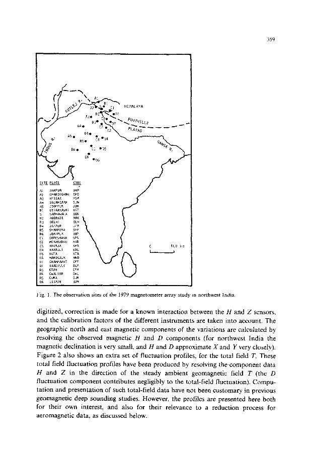
Fig. 1. The observation sites of the 1979 magnetometer array study in northwest India.

digitized, correction is made for a known interaction between the H and Z sensors, and the calibration factors of the different instruments are taken into account. The geographic north and east magnetic components of the variations are calculated by resolving the observed magnetic H and D components (for northwest India the magnetic declination is very small, and fif and D approximate X and Y very closely). Figure 2 also shows an extra set of fluctuation profiles, for the totai field T. These total field fluctuation profiles have been produced by resolving thecomponent data H and Z in the direction of the steady ambient geomagnetic field T (the D fluctuation component contributes negligibly to the total-field fluctuation). Compu- tation and presentation of such total-field data have not been customary in previous geomagnetic deep sounding studies. However, the profiles are presented here both for their own interest, and also for their relevance to a reduction process for aeromagnetic data, as discussed below.

Fig. 2. Stacked variometer profiles for the substorm event of 5 April 1979. starting at I.559 U.T.

approxrmately. and of 102 min. duration. The notations X, Y and Z denote the magnetic fluctuation

components in the directions of geographic north, east and vertically downwards. The notation T denotes

the magnetic fluctuation component resolved in the direction of the local ambient main geomagnetic field.

as would be measured by a total-field magnetometer. Note that the components are not all plotted to the

same vertical scale.

361

The stacked profiles in Fig. 2 summarize much information. The strongest

geophysical effect is perhaps in the contrasts between the vertical component (Z)

signals at certain stations, for example where a complete reversal of the fluctuation

characteristic is seen between sites B2 (Roorkee) and 03 (Etah). This phenomenon,

occurring consistently as it does for a number of substorms, indicates a concentra-

tion of induced current flow inside the ground along a path running through

between these two stations.

The horizontal components in Fig. 2 also show departures from uniformity, and

are marked by their surplus strength where anomalously strong ground currents are

flowing beneath some of the recording stations.

Response arrows determined

Following a widely used procedure for the analysis of magnetic fluctuation data

(Schmucker, 1964, 1970; Everett and Hyndman, 1967), anomalous vertical-compo-

nent (Z) signals apparent at many of the stations in Fig. 2 are found to be related to

the horizontal-component signals X and Y by the simple equation:

Z=AX+BY (1)

where A and B are functions of geographical position and A, B, X, Y and Z are all

functions of the frequency of magnetic fluctuations, and are complex with real and

quadrature parts. The functions A and B ideally are determined by earth electrical

conductivity structure. While particular theoretical models predict that eq. 1 will be

obeyed, its application to general data is an empirical approach. Substorm events of

different polarization characteristics are needed to make good determinations of the

A and B functions, and if A and B are to be interpreted in terms of geological

structure, care must be taken to minimize any biassing effect on their determination

that non-uniform source field effects might have.

Values of A and B thus determined may be combined to form arrows which,

plotted on a map, indicate regions of anomalously high electrical conductivity by

pointing towards paths of current concentration in the ground. In the present work,

separate arrows are constructed for both the real and quadrature parts of A and B,

and following the convention of Parkinson (1962) such arrows are plotted with

components A south and B west.

Such a set of arrows, for a period of 91 min, is shown for the northwest Indian

array in Fig. 3 (from Arora et al. 1982), superimposed on a sketch map of some main

tectonic features of India. In the determination of the arrows shown in Fig. 3, the

horizontal fields X and Y in eq. 1 above have been taken as those at Karauli (C4); if

Karauli records were not available then those at Khurja (C3) or ,Kota (C5) were used.

Interpretation in terms of conductive structures

Conductive structures marked Z-I/I are shown in Fig. 3. These structures have

been interpreted not only from the arrows shown, but also from arrow patterns at

t’lg. 3. Map of Indta. showmg real Parkinson arrows determined for magnetic fluctuations of yl-mm

period. with superimposed the interpreted conductive structures I cif. The positioning of structure /I i\

prtwrs~cmal. Structurrs 1 and II are clasacd as “first order”. and structures ill- 17 we ciasscd DA “second

cvder”.

shorter periods, and particularly from maps of Fourier transform parameters ob-

tained from the response of different stations to substorms such as that shown in

Fig. 2. More arrow patterns, and several sets of such Fourier transform parameter

maps. are given in Arora et al. (1982).

There are two “first-order” structures. marked I and II. The position of structure

I is relatively well-controlled by the array stations. The structure strikes across the

Ganga Basin, at a depth of the order of 50 km. and is interpreted as a continuation

of the Aravalh Belt being thrust down by the collision of India and Asia, and made

highly conductive by the conditions of stress and temperature which it is experienc-

ing.

The presence of structure II to the west of the array area is indicated by the

consistent westward-pointing arrow pattern for stations in the southern half of the

363

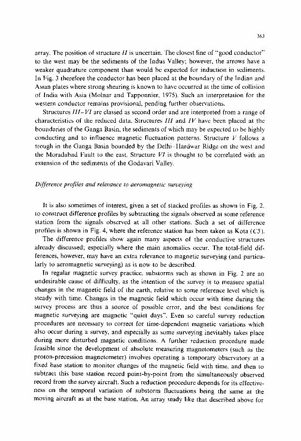
array. The position of structure ZZ is uncertain. The closest line of “good conductor”

to the west may be the sediments of the Indus Valley; however, the arrows have a

weaker quadrature component than would be expected for induction in sediments.

In Fig. 3 therefore the conductor has been placed at the boundary of the Indian and

Asian plates where strong shearing is known to have occurred at the time of collision

of India with Asia (Molnar and Tapponnier, 1975). Such an interpretation for the

western conductor remains provisional, pending further observations.

Structures III- VI are classed as second order and are interpreted from a range of

characteristics of the reduced data. Structures ZZZ and II/ have been placed at the

boundaries of the Ganga Basin, the sediments of which may be expected to be highly

conducting and to influence magnetic fluctuation patterns. Structure V follows a

trough in the Ganga Basin bounded by the Delhi-Hardwar Ridge on the west and

the Moradabad Fault to the east. Structure VI is thought to be correlated with an

extension of the sediments of the Godavari Valley.

Difference profiles and relevance to aeromagnetic surveying

It is also sometimes of interest, given a set of stacked profiles as shown in Fig. 2,

to construct difference profiles by subtracting the signals observed at some reference

station from the signals observed at all other stations. Such a set of difference

profiles is shown in Fig. 4, where the reference station has been taken as Kota (0).

The difference profiles show again many aspects of the conductive structures

already discussed; especially where the main anomalies occur. The total-field dif-

ferences, however, may have an extra relevance to magnetic surveying (and particu-

larly to aeromagnetic surveying) as is now to be described.

In regular magnetic survey practice, substorms such as shown in Fig. 2 are an

undesirable cause of difficulty, as the intention of the survey is to measure spatial

changes in the magnetic field of the earth, relative to some reference level which is

steady with time. Changes in the magnetic field which occur with time during the

survey process are thus a source of possible error, and the best conditions for

magnetic surveying are magnetic “quiet days”. Even so careful survey reduction

procedures are necessary to correct for time-dependent magnetic variations which

also occur during a survey, and especially as some surveying inevitably takes place

during more disturbed magnetic conditions. A further reduction procedure made

feasible since the development of absolute measuring magnetometers (such as the

proton-precession magnetometer) involves operating a temporary observatory at a

fixed base station to monitor changes of the magnetic field with time, and then to

subtract this base station record point-by-point from the simultaneously observed

record from the survey aircraft. Such a reduction procedure depends for its effective-

ness on the temporal variation of substorm fluctuations being the same at the

moving aircraft as at the base station. An array study like that described above for

364

c 3 .._--__r-----_---- -v%“\,/._ m .--- ~‘\,.,x_,eL_ ----w-L_-,-----

cs ____. ___.__ - _-... ____ ___I -..--___..~_._

Fig. 4. Stacked difference profiles. obtained from the data of Fig. 2 by subtracting the appropriate

component recorded at Kota (C’S) from the records of every other station. Note that as in Fig. 2 the

components are not all plotted to the same vertical scale. Note also particularly some large contrasts in

the T profiles. for example between Al (Rampur) and AZ (Chandigarh), so that a total-field base station

at the former site would give a poor estimate of total-field fluctuations occurring at the latter site.

365

northwest India shows the extent to which this condition holds over areas of the

scale of those covered by an aeromagnetic survey.

In particular, the total-field profiles of Fig. 4 indicate differences relative to a

base station at Kota (C.5). It can be seen that away from the main electrical

conductivity anomaly (structure I) the differences are relatively weak, with maxima

for the substorm shown of order 5 nT, whereas near the anomaly there are times

when differences arise of the order of 30 nT. The point demonstrated is that

aeromagnetic surveys in areas of conductivity anomaly (and in the case of northwest

India near structure I) may require extra care in the data reduction process,

especially for data recorded at times other than those of magnetic quiet. Subtracting

the record of a fixed base station from a survey record may not be an effective way

of correcting for substorm temporal variation in areas of electrical conductivity

anomaly.

Comments on the results of the northwest India array study

Although much numerical computation has been necessary in the production of

the stacked profiles and arrow patterns presented in this paper, the interpretation

given above is basically qualitative: that particular electrical conductivity anomalies

have been discovered. Such results are entirely appropriate for a reconnaissance

study. Future field observations may well expand the boundaries of the area

covered, and also occupy a denser network of stations in the regions now shown to

be of interest.

The numerical modelling of such observed field data to derive an interpretation in

terms of quantitative electrical conductivity structures is a major frontier in present-

day geomagnetic research. Some important theoretical problems are involved, per-

haps most notably the extent of the “induction region” for an anomaly such as that

associated with structure I. Is the current concentrated in structure I induced locally,

or is it induced much more widely (even globally) and channelled in the structure I

like a large-scale steady-current flow? For the case of structure 1 there is also the

important question of how far into the mountains does the electrical conductivity

anomaly extend.

THE MAGNETOMETER ARRAY STUDY IN SOUTH INDIA

Sites

The station sites for the instruments of the second array experiment in south

peninsular India are shown in Fig. 5. The array was operated with the same 21

Gough-Reitzel type magnetometers of the Australian National University, Canberra,

as the northwestern array. Installation of the temporary observatories in south India

was carried out between September and December 1979, and the instruments

PENINSULAR INDIA

(Magnetic Array Stations1

**

I AN

Fjg. 5. Magnetic array stations of the second experiment m south peninsular India operated during

September 1979-March 1980.

operated simultaneously between December 1979 and March 1980. As before. the

instruments made observations at l-mm intervals of the three components N, D and

Z.

The array data were further supplemented with simultaneous records from five

permanent magnetic observatories operating in the region.

Some of the important results of this array experiment are described in detail by

Thakur et al. (1981) and Srivastava et al. (1982). Analysis and interpretation of the

array data are still in progress.

Stacked profiles of u magnetic substorm event

In the southern array again, a variety of quiet-day and magnetic disturbance

events was recorded. One night-time substorm is reproduced in Fig. 6, and another

in Fig. 7.

In the region of southern peninsular India, the source field is highly non-uniform

during day hours due to the presence of the equatorial electrojet over the dip

367

r

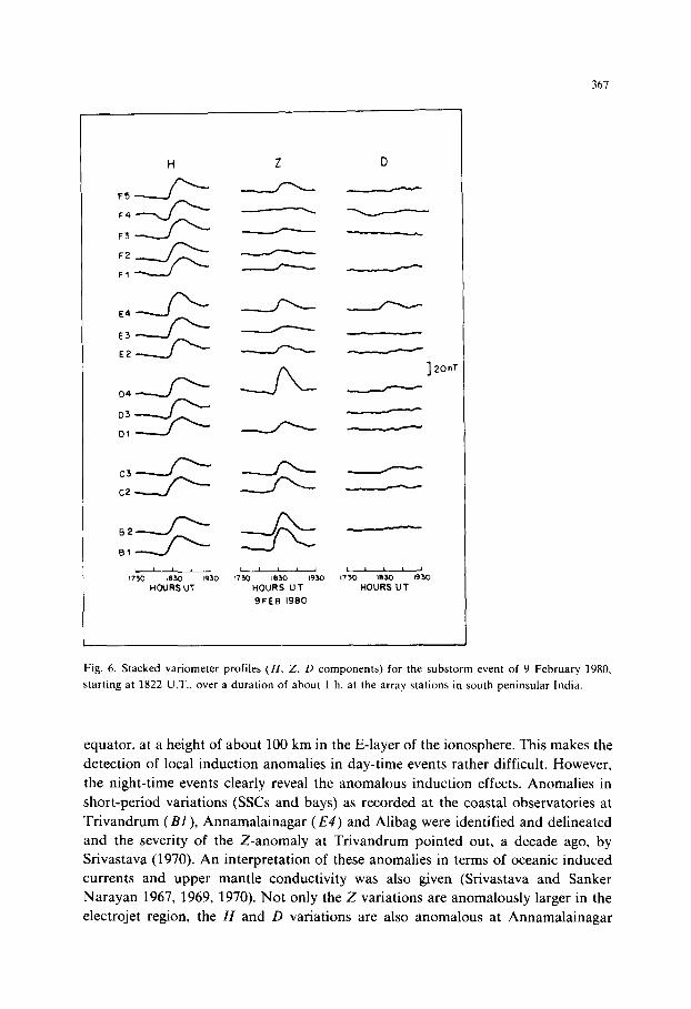
Fig. 6. Stacked variometer profiles (H, Z, D components) for the substorm event of 9 February 1980,

starting at 1822 U.T.. over a duration of about 1 h. at the array stations in south peninsular India.

equator, at a height of about 100 km in the E-layer of the ionosphere. This makes the

detection of local induction anomalies in day-time events rather difficult. However,

the night-time events clearly reveal the anomalous induction effects. Anomalies in

short-period variations (SSCs and bays) as recorded at the coastal observatories at

Trivandrum (Bl ), Annamalainagar (E4) and Alibag were identified and delineated

and the severity of the Z-anomaly at Trivandrum pointed out, a decade ago, by

Srivastava (1970). An interpretation of these anomalies in terms of oceanic induced

currents and upper mantle conductivity was also given (Srivastava and Sanker

Narayan 1967, 1969, 1970). Not only the Z variations are anomalously larger in the

electrojet region, the H and D variations are also anomalous at Annamalainagar

D

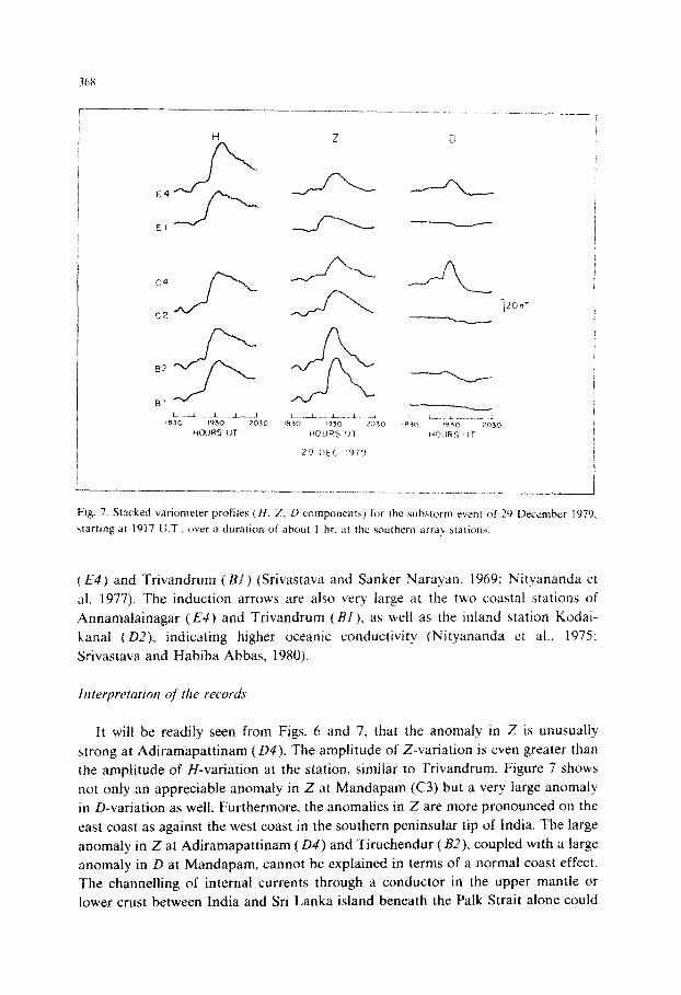
Fig. 7. Stacked vartometer profiles (/f. Z, D components) for the suhstorm event of 29 December 1979.

htarting at 1917 U.T.. over a duratrnn of about 1 hr. ;tt the southern arm! stattons.

(E4) and Trivandrum (BI ) (Srivastava and Sanker Narayan, 1969: Nityananda et

al. 1977). The induction arrows are also very large at the two coastal stations of

Annamalainagar (E4) and Trivandrum (Et! ), as well as the inland station Kodai-

kanal (D2), indicating higher oceanic conductivity (Nityananda et al., 197.5:

Srivastava and Habiba A&as, 1980).

Interprrtcrtion of the twords

It will be readily seen from Figs. 6 and 7. that the anomaly in Z is unusual1~

strong at Adiramapattinam (04). The amplitude of Z-variation is even greater than

the amplitude of ~-variation at the station, simiIar to ~rrivandrum. Figure 7 shows

not only an appreciable anomaly in Z at Mandapam (C3) but a very large anomaly

in D-variation as well. Furthermore. the anomalies in Z are more pronounced on the

east coast as against the west coast in the southern peninsular tip of India. The large

anomaly in Z at Adiramapattinam (04) and Tiruchendur (B2). coupled with a large

anomaly in D at Mandapam, cannot be explained in terms of a normal coast effect.

The channelling of internal currents through a conductor in the upper mantle or

lower crust between India and Sri Lanka island beneath the Palk Strait alone could

369

give rise to such large induction anomalies (Nityananda et al., 1977; Rajaram et al.,

1978). The question of anomalously large Z-variations and the suppression of

H-variations in the equatorial electrojet region of India as compared to the Ameri-

can region can also be resolved partly by assuming induced currents channelling

between India and Sri Lanka.

The geological conductor seems to be associated with the India-Sri Lanka graben

(a triple junction rift) suggested by Naqvi et al. (1974) and Burke et al. (1978). The

geomagnetic observations suggest that the conductor has a north-south trend near

Mandapam (C3) and is quite close to it since it affects the D-variations severely.

Larger Z-variations on the east coast could be due to its closeness to the Pondicherry

rift. A conductive step structure at the Moho boundary along the coast in the

southern peninsular region and the associated current concentration therein, along

with the induced currents in the sea water, would also make significant contributions

to the observed anomalous geomagnetic variations (Srivastava and Habiba Abbas,

1980).

CONCLUDING REMARKS

The Indian sub-continent contains strong electrical conductivity contrasts, and

the unravelling of its electric current path connections with the oceans and with Asia

provides an important geophysical challenge. In stimulating the investigation of such

problems, the Indian magnetometer array studies complement similar projects taking

place in other continents.

There is another point regarding interpretation philosophy which may ap-

propriately be made here. In the trial stages of magnetometer arrays, as of any new

development, it is natural to accept results only to the extent that they agree with

what is already known of geologic structure. However, for a new development to

produce new information it is ultimately necessary for the results of the development

to be accepted on their own basis. Magnetometer array studies may now be at this

stage, giving information on electrical conductivity structure in the lithosphere and

asthenosphere which is not obtainable in any other way.

GDS and MT studies are also desirable in the regions of the Deccan Traps, the

Narmada, Godavari and Koyna rifts, the Cuddapah basin, the southern tip of the

Indian peninsula together with Sri Lanka, and the syntaxial zones of the Kashmir

Himalaya and the Assam Himalaya. The studies in the Himalaya will also bring out

the association of induction anomalies with seismicity and plate margins. Analogue

and theoretical model studies of the various situations encountered in the induction

problem in India are also necessary for better appreciation and interpretation of the

observations in terms of lithospheric parameters.

ACKNOWLEDGEMENTS

The magnetometer array studies described here were carried out under the

India-Australia Science and Technology Agreement, in which Dr. Hari Narain and

370

Prof. B.N. Bhargava played a key role as Indian National C’oordinatora. .I he authorx

thank the many people who have helped with the necessary administration of such ;I

large project, and also those who assisted in the field with the in~tallatlon and care

of the recording instruments. We acknowledge particularlv the contributions of Dr.

S.N. Prasad, Dr. A.V. Ramana Rao and Mr.S.B. Gupta of the National (&physical

Research Institute, Hyderabad and Dr. B.R. .4rora. Mr. M.V. Mahashabdc. Mr.

N.K. Thakur and Mr. V.H. Badshah of the Indian Institute of <;eomagnetism.

Bombay. We thank Mrs. M.N. Sloane for her part in the work of the project carried

out at the Australian National University, Canberra.

We thank particularly the Directors of our respective home institutes for their

encouragement and assistance. Especially in this volume we pay tribute to Dr. Hari

Narain. for his work in the leadership of geophysics. both Indian and international.

RbFERENCES

Arora. B.R.. Lilley. F.F..M.. Sloane. M.N.. Slngh. B.P.. Srlvasta\a. B.J. and Prasad. S.%.. 19X2. Geomag-

netlc induction and conductive \tructures in northwest India. C;eophw. J.R. A\tron. Sot.. 69:

4s’) -475.

Burke. K.C.A.. Delano. L.. Dewey, J.t:., Edelatem. A.. Kldd, W.S.F.. Nelxm. K.D.. Sengor. A.M.C’. and

Strup. J.. 1978. Rifts and sutures of the world. Contract Rep. NAS 5-24094. Geophys. Branch, ESA

Div.. Goddard Space Flight Center. Greenbelt. Md.. 238 pp.

Chapman. S.. 1919. The solar and linear diurnal variatwna of the earth’s magnetism. Phtb. Trans. R.

Sot. London. Ser. A., 21X: I-1 IX.

Chapman. S.. 1967. Perspective. In: S. Matsushita and W.H. Campbell (Editors). Ph>alcs of Geomagnetic

Phenomena. Academic Press. New York. pp. B-28.

Chapman. S. and Whitehead, T.-T.. 1922. The influence of electrically ccmducting material wthin the earth

on various phenomena of terrestrial magnetism. Trans. Philos. Sot. Cambridge. 22. 463-4X2.

Everett. J.E. and Hyndman. R.D.. 1967. Geomagnetic variation:, and electrical conductivity structure 111

south-western Australia. Phya. Earth Planet. Inter.. I : 24-34.

Hutton. V.R.S.. 1976. The electrical conductivity of the earth and planets. Rep. Prog. Phys.. 39: 4X7- S72.

Lahlri. B.N. and Prtce. A.T.. 1939. Electromagnetic induction in non-uniform conductor\ and the

determination of the conductivity of the earth from terrestrial magnetic variations. Philns. Trans. R.

Sot. London. Ser. A. 237: SO9- 540.

Lilley. F.E.M., Burden. F.R.. Boyd. G.W. and Sloane. M.N.. 1975. Performance test\ of a set of

Gough-Reitzel magnetic variometers. J. Geomagn. Geoelectr.. 27: 75-83.

Lllle), F.E.M.. Slngh. B.P.. Arora. B.R.. Srivastava. B.J.. Prasad. S.N. and Sloane. M.N.. 19X1. A

magnetometer array study in northwest India. Phys. Earth Planet. Inter.. 25: 232-240.

Molnar. P. and Tapponnier. P.. 1975. Cenozoic tectonics of Asia: effects of a continental collision.

Science. 1 X9: 419--426.

Moos. N.A.F.. 1910. CoIaba Magnetic Data (1846-1905). Part I. Magnetic Data and Instruments. Part II.

The Phenomenon and its Discussion. 782 pp.

Naqvi. SM.. Rae. V.D. and Narain, II.. 1974. The protocontmental growth of the lndlan stueld and the

anlqtnty of its rift valleys. Precambrian Rea.. 1 : 345. 39X.

Nityananda, N.. Rajagopal. PI.%. Agarwal. A.K. and Singh, B.P.. 1975. Induction In short-period events in

the Indian peninsula. Proc. Symp. tquat. Geomagn. Phen.. I.I.G.. Bomhay. pp. 16X 172.

Nityananda, N.. AgarwaI. A.K. and Sir&. B.P., 1977. Induction at short periods in the horizontal

variations in the Indian Peninsula. Phys. Earth Planet. Inter., 15: P5mP9.

771

Schmuckcr. L.. lY5Y. Erdmagnrt~xhc T~efcnwndwung 111 L)euixhl:~nd lY57 5Y. hla~ncIc)yammc und

c‘rlrtr‘ Ausuerlung. Ahh. Ahad. W~ss. Golrlngcn. Math.-Ph)\. KI.. Sonderh. 3. Hcltr.qx ,um l.<i.‘~‘.. 5.

Schmuckcr. L.. 1964. Anomatic~ of gec>mJgnctlc varlatwn\ 111 lhc \<wrh-ueicrn l~n~rsd SI.IIC\. J.

Gec>magn. (;coeteclr.. 15: 192-221.

Schuster. A.. IXXY. The diurnal \drlauon of terrr‘\trlal magncrlsm. wih an appwd~x h\ II. L.imh “On ihc‘

current\ Induced In a \pherlcul cc)nduclor h\ \*arlaticnl of .~n cr;lc’rn;II m.lgncllc potrntlal”. I’hllclr.

Tram. K. Sot. London. Ser.. ,A. 1X0: 467 -51X.

Srlvaava. B.J.. 1966. The H!derahatl gccm~apnerlc ~JILL Ior Ihr kcar 1Y65 .I ccmlpJrl\<,n ;q+i~n>r Ihe

Ahhag dais Fc)r 1945. lY55 and IYSX. Hull. N.G.K.1.. 4: IIY 122.

Srlraaiva. H.J.. 1970. tnlcrccmpJrlwn of magnclomclrr mcawrcmcnl~ 111 tndla end 115 Irnpllcallon~.

Prtx. S)mp. Prohh. I:quut. I:lcctroJet. Ahm&had. X Auguhi lY70. P.I~. So. I I. Srlvasrava. H.J. and tlahlha AhhJ\. 19X0. An In1crprcl;iuon ot the InductlcJn arrw.3 at 1nd1.1n \I:IIICVI\. J.

Gcomagn. ~;eocleclr.. 32 (Supp. I): SI 1X7. SI IYh.

Srivatava. B.J. and Sankcr Narayan. P.V.. 1970. Anomalou\ geomagncllc var~atwr~~ In rhc t’enln\ular

India-Occdn efkt and upper manllr conducliwl> hlruclurc. Hull. N.G.K.I.. X: 175-134.

Swwaw. H.J.. Bhaskara Rae. D.S. and Praaad. S.N.. lY74a. Gecmagnellc Induction .mom.~tlc’., along Ihe

llkdcrahad Kalingapatnam profllc. Teclonoph~w\. 24: 343-35~.

SrlLaslaka. H.J.. Bhaskara Rae. I1.S. and Praad. S.N.. lY74h. <;com;lgnctlc v;lrl:illon Jnc~mJtle5 In t)lc

Koynna and Ihe Bhadrachaldm sc’lhmlc drea\ In Prmnsular India. J. Gccmagn. <;eortrctr.. 26. 247. 2~5.

Srwasrava. H.J.. Prasad. S.N.. Slngh. 13.P.. Arora. B.R.. Thahur. N.K. and hlahaahahde. k1.V.. IYX?.

tnducllon xmmatws In grom.qywtlc Sq In penlnwlar India. C;a~ph~\. KC\. Leti.. 9: 1125- 1 \ 3x. Thdkur. N.K.. Mahashabdc. hf.\'.. Arora. B.K.. Slngh. B.I’.. Srl\u\la\a. B.J. and Pr.lhad. S.N.. 1YXt.

.AnOmalw in geomagnellc varl.illons on penlnwlnr tndla ns.ir P.111, \lr;i1!. (;e,>ph\3. Kc,. t.e~t.. X:

947 950.