Magnetic Field Structure of Dense Cores Using Spectroscopic Methods

Sayantan Auddy1,2 , Philip C. Myers1 , Shantanu Basu2 , Jorma Harju3,4 , Jaime E. Pineda3 , and Rachel K. Friesen51 Harvard-Smithsonian Center for Astrophysics, 60 Garden Street, Cambridge, MA 02138, USA; sauddy3@uwo.ca

2 Department of Physics and Astronomy, The University of Western Ontario, London, ON N6A 3K7, Canada3 Max-Planck-Institute for Extraterrestrial Physics (MPE), Giessenbachstr. 1, D-85748 Garching, Germany

4 Department of Physics, P.O. Box 64, FI-00014 University of Helsinki, Finland5 National Radio Astronomy Observatory, Charlottesville, VA 22903, USA

Received 2018 September 21; revised 2018 December 22; accepted 2019 January 18; published 2019 February 26

Abstract

We develop a new “core field structure” (CFS) model to predict the magnetic field strength and magnetic fieldfluctuation profile of dense cores using gas kinematics. We use spatially resolved observations of the nonthermalvelocity dispersion from the Green Bank Ammonia survey along with column density maps from SCUBA-2 toestimate the magnetic field strength across seven dense cores located in the L1688 region of Ophiuchus. The CFSmodel predicts the profile of the relative field fluctuation, which is related to the observable dispersion in thedirection of the polarization vectors. Within the context of our model, we find that all of the cores have atranscritical mass-to-flux ratio.

Key words: ISM: clouds – ISM: magnetic fields – stars: formation

1. Introduction

Stars form in dense cores embedded within interstellarmolecular clouds (Lada et al. 1993; Williams et al. 2000; Andréet al. 2009). Dense cores are well studied observationally frommolecular spectral line emission (Myers & Benson 1983;Benson & Myers 1989; Jijina et al. 1999), infrared absorption(Teixeira et al. 2005; Lada et al. 2007; Machaieie et al. 2017),and submillimeter dust emission (Ward-Thompson et al. 1994;Kirk et al. 2005; Marsh et al. 2016).

Cores may form in multiple ways including fragmentation ofover-dense regions that are typically filaments and sheets (Basuet al. 2009a, 2009b) within turbulent magnetized clouds.Depending on the ambient initial conditions, they can formeither as a result of spontaneous gravitational contraction (Jeans1929; Larson 1985, 2003) or by rapid fragmentation due topreexisting turbulence (Padoan et al. 1997; Klessen 2001;Gammie et al. 2003). Another scenario is the formation of coresin magnetically supported clouds due to quasistatic ambipolardiffusion, i.e., gravitationally induced drift of the neutral specieswith respect to ions (Mestel & Spitzer 1956; Mouschovias 1979;Shu et al. 1987). However, a more recent view is that bothsupersonic turbulence and gravitationally driven ambipolardiffusion are significant in the process of core formation (e.g.,Nakamura & Li 2005; Kudoh & Basu 2011, 2014; Chen &Ostriker 2014; Auddy et al. 2018).

Dense cores often have nonthermal contributions to linewidth that are small compared to the thermal values (Rydbecket al. 1977; Myers 1983; Caselli et al. 2002). Theseobservations imply a transition from a primarily nonthermalline width in low-density molecular cloud envelopes to a nearlythermal line width within dense cores. This is termed as “atransition to velocity coherence” (Goodman et al. 1998). Asharp transition between the coherent core and the denseturbulent gas surrounding the B5 region in Perseus was foundusing NH3 observations from the Green Bank Telescope (GBT)by Pineda et al. (2010). It has been suggested that this transitionarises from damping and reflection of MHD waves (Pinto et al.2012).

An important question is whether a transition from magneticsupport of low-density regions to gravitational collapse ofdense regions is physically related to the transition tocoherence. Furthermore, how is the magnetic field strengthaffecting the nonthermal line width in the low-density region,and is this related to the velocity transition? If so, can oneestimate the magnetic field strength and its radial variationacross a dense core using such observations?Accurate measurement of the magnetic field is one of the

challenges of observational astrophysics. Several methods existthat probe the magnetic field in the interstellar medium, such asZeeman detection (e.g., Crutcher 1999), dust polarization(Hoang & Lazarian 2008), and Faraday rotation (Wolleben &Reich 2004). While each method has its own limitations(Crutcher 2012), sensitive observations of dust polarization candescribe the structure of the plane-of-sky magnetic field andcan estimate its strength. According to the dust alignmenttheory (Andersson et al. 2015), the elongated interstellar dustgrains tend to align with their minor axis parallel to themagnetic field. Dust polarization observations from thermalemission or extinction of background starlight provide a uniqueway to probe the magnetic field morphology in the ISM,including collapsing cores in molecular clouds.In addition to getting the field morphology, there are various

methods to estimate the magnetic field strength. One of thepopular techniques is the Davis–Chandrasekhar–Fermi (DCF)method (Davis & Greenstein 1951; Chandrasekhar &Fermi 1953) that estimates the field strength using measure-ments of the field dispersion (about the mean field direction),gas density, and one-dimensional nonthermal velocity disper-sion. Dust polarization, however, can be weak in the centers ofdense cores where the dust grains are well shielded from theradiative torques necessary to move the grains into alignmentwith the magnetic field (e.g., see Lazarian & Hoang 2007).Recently, Myers et al. (2018) have extended the spherical

flux-freezing models of Mestel (1966) and Mestel & Strittmatter(1967) to spheroidal geometry, allowing quantitative estimatesof the magnetic field structure in a variety of spheroidal shapesand orientations. In these models, the magnetic field energy in

The Astrophysical Journal, 872:207 (13pp), 2019 February 20 https://doi.org/10.3847/1538-4357/ab0086© 2019. The American Astronomical Society. All rights reserved.

1

the spheroid is weaker than its gravitational energy, allowinggravitational contraction, which drags field lines inward.However, the spheroid magnetic field energy is stronger thanits turbulent energy, allowing the field lines to have an ordered“hourglass” structure. These models are useful to test clouds,cores, and filaments that show ordered polarization for theprevalence of flux freezing. They also allow an estimate of themagnetic field structure when the underlying density structure issufficiently simple and well known.

The present paper is complementary to Myers et al. (2018)since it relies on many of the same assumptions of flux freezingin a centrally condensed star-forming structure. However, it ismore specific to dense cores having subsonic line widths. Italso relies on additional information, i.e., maps of nonthermalline widths, and on the additional assumption that thenonthermal line widths are due to Alfvénic fluctuations in themagnetic field lines, as in the original studies of DCF.

In this paper, we predict magnetic field structure byanalyzing new NH3 observations of multiple cores in theL1688 region in the Ophiuchus molecular cloud. Most of thecores show a sharp transition to coherence with a nearlysubsonic nonthermal velocity dispersion in the inner region.We propose a new “Core Field Structure” (CFS) model ofestimating the amplitude of magnetic field fluctuations. Itincorporates detailed maps from the Green Bank AmmoniaSurvey (GAS) of the nonthermal line width profiles across acore. The paper is organized in the following manner. Theobservations of the gas kinematics and the column density arereported in Section 2. In Section 3, we introduce the CFSmodel and the inferred magnetic field profile. In Section 4, wediscuss the limitations of the model. We highlight some of theimportant conclusions in Section 5.

2. Observations

The first data release paper from the GBT survey (Friesenet al. 2017) included detailed NH3 maps of the gas kinematics(velocity dispersion, σv and gas kinetic temperature, TK) of fourregions in the Gould Belt: B18 in Taurus, NGC 1333 inPerseus, L1688 in Ophiuchus, and Orion A North in Orion. The

emission from the NH3 (J, K )=(1, 1) and (2, 2) inversionlines in the L1688 region of the Ophiuchus cores were obtainedusing the 100 m GBT. The observations were done using in-band frequency switching with a frequency throw of 4.11MHz,using the GBT K-band (upper) receiver and the GBTspectrometer at the front and back end, respectively. L1688is located centrally in the Ophiuchus molecular cloud. It is aconcentrated dense hub (with numerous dense gas cores)spanning approximately 1–2 pc in radius with a mass of

M2 103´ (Loren 1989). L1688 has over 300 young stellarobjects (Wilking et al. 2008) and contains regions of highvisual extinction, with AV∼50–100 mag (e.g., Wilking &Lada 1983). The mean gas number density of L1688 isapproximately a few 10 cm3 3´ - .Submillimeter continuum emission from dust shows that the

star formation efficiency of the dense gas cores is ≈14%(Jørgensen et al. 2008). Figure 1 (modified from Figure 6 inFriesen et al. 2017) shows the integrated intensity map of theNH3(1, 1) line for the L1688 region in Ophiuchus, along withthe marked cores that are studied in this paper. The mapincludes four prominent isolated starless cores (includingH-MM1 and H-MM2) lying on the outskirts of the cloud, plusmore than a dozen local line width minima in the main cloud(mainly in the south-eastern part in regions called Oph-C, E,and F). Many of these minima correspond to roundish starlesscores that can be identified on the SCUBA-2 850 micron dustcontinuum map. The cores indicated as Oph-C, Oph-CN, Oph-E, and Oph-FE correspond to source names C-MM3, C-MM11,E-MM2d, and F-MM11, respectively, as mentioned in Pattleet al. (2015). Furthermore, Oph-C, Oph-E, and HMM-1 areclassified as starless, while the other cores are known to have aprotostar (see Table 1 in Pattle et al. 2015 for more coreproperties).

2.1. Velocity Dispersion

The radial distributions of the velocity dispersions and thekinetic temperatures were calculated from aligned and averagedNH3(1, 1) and NH3(2, 2) spectra. The averages were calculatedin concentric annuli, weighting the spectra by the inverse of therms noise (for example see Figure 12, which demonstrates

Figure 1. Integrated intensity map of the NH3(1, 1) line for the L1688 regiontaken from Friesen et al. (2017). The beam size and scale bar are shown in thebottom left and right corners, respectively. The cores studied in this paper areindicated by name.

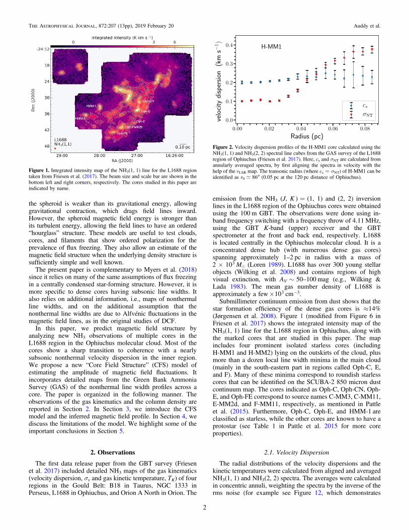
Figure 2. Velocity dispersion profiles of the H-MM1 core calculated using theNH3(1, 1) and NH3(2, 2) spectral line cubes from the GAS survey of the L1688region of Ophiuchus (Friesen et al. 2017). Here, cs and σNT are calculated fromannularly averaged spectra, by first aligning the spectra in velocity with thehelp of the vLSR map. The transonic radius (where cs=σNT) of H-MM1 can beidentified as r0;86″ (0.05 pc at the 120 pc distance of Ophiuchus).

2

The Astrophysical Journal, 872:207 (13pp), 2019 February 20 Auddy et al.

annular averaging of spectra for the H-MM1 core). Before theaveraging, the spectra were aligned in velocity using LSRvelocity maps produced by the reduction and analysis pipelinefor the Greenbank K-band Focal Plane Array Receiver (Masterset al. 2011; Friesen et al. 2017).6

The stacked NH3(1, 1) and (2, 2) spectra were analyzedusing the standard method described by Ho & Townes (1983)and, recently, by Friesen et al. (2017). In this method, thevelocity, line width, the total optical depth, and the excitationtemperature of the (1, 1) inversion line are determinedsimultaneously by fitting a Gaussian function to the 18hyperfine components. The assumption is that individualhyperfine components have equal excitation temperatures,Tex, beam-filling factors, and line widths.

The column density of molecules in the (J=1, K=1) leveldepends on Tex and is proportional to the product of the linewidth and the total optical depth. The (2, 2) inversion line isusually optically thin, and the column density of the moleculesin the (J=2, K=2) level is estimated using the integratedintensity of the (2, 2) inversion line. It is assumed that the (2, 2)inversion line has the same dependence on Tex and has thesame relation to the line width as the (1, 1) line. The ratio of thecolumn densities of the J, K=(1, 1) and (2, 2) levels definesthe rotation temperature, Trot. The kinetic temperature Tkin wasestimated using the three-level approximation, including levelsJ, K=(1, 1), (2, 2), and (2, 1), as described by Walmsley &Ungerechts (1983) and Danby et al. (1988).

The nonthermal velocity dispersion in an averaged spectralline was calculated by subtracting in quadrature the thermalvelocity dispersion of ammonia molecules from the total

velocity dispersion. The errors of the thermal and nonthermalvelocity dispersions were calculated by propagating theuncertainties of the variables derived from the averagedspectra. Here, it is assumed that the error in Tkin does notcorrelate with that of the line width. The dominant uncertaintiesin the Tkin estimate are related to the optical thickness of the(1, 1) line (depending on the relative intensities of the hyperfinecomponents) and the integrated intensity of the (2, 2) line.The relative error of the line width is usually very small (a fewpercent) and has a minor effect on the uncertainty in Tkin.Figure 2 shows the radially averaged isothermal sound speed

cs and nonthermal velocity dispersion σNT in HMM-1. Here,c kT ms Hm= where T is the kinetic temperature, mH is themass of a hydrogen atom, and μ=2.33 is the mean molecularmass. Furthermore, v 2 ln 2NT NTs = D , and ΔvNT is thenonthermal contribution to the NH3 line width. There is a cleartransition point at radius ≈86″, where cs NTs= . We identifythis radius as the transonic radius, rc, and consider it to be thecore boundary. The nonthermal velocity dispersion is ≈0.5csinside the core, and it increases steeply to ≈2cs across the coreboundary. We use the same prescription to map the thermal andnonthermal velocity dispersion of six other selected cores inL1688. Figure 3 shows the annularly averaged thermal andnonthermal velocity dispersions of all the other selected cores inL1688. We have selected only those cores that have a distinctdelineation between thermal/nonthermal line widths (cs=σNT)at a transonic radius rc with the nonthermal dispersion becomingsubthermal toward the center of the core. Outside the transonicradius for some cores (for example Oph-CN and Oph-Fe), thenonthermal dispersion is comparable to the sound speed.In Table 1, we give the measure of the transonic radius rc

and the corresponding velocity dispersion (σNT)c at rc. Thevalues of rc and (σNT)c are obtained by interpolating the

Figure 3. Velocity dispersion profiles of some selected cores in Ophiuchus calculated using the NH3(1, 1) and NH3(2, 2) spectral line cubes from the GAS survey ofthe L1688 region of Ophiuchus (Friesen et al. 2017). Here, cs and σNT are calculated from annularly averaged spectra, by first aligning the spectra in velocity with thehelp of the vLSR map.

6 The data are available throughhttps://dataverse.harvard.edu/dataverse/GAS_DR1.

3

The Astrophysical Journal, 872:207 (13pp), 2019 February 20 Auddy et al.

thermal and nonthermal data points and finding theirintersection.

2.2. Column Density and Density Model

Figure 4 shows the circularly averaged 850 μm intensityprofiles of seven cores in L1688 derived from SCUBA-2 maps(see Figure 1 in Pattle et al. 2015). In order to characterize eachobserved column density profile, we adopt an idealizedPlummer model of a spherical core (Arzoumanian et al.2011) with radial density

rr r1

, 1p

0

02 2

rr

=+

( )[ ( ) ]

( )

where the parameter r0 is the characteristic radius of the flatinner region of the density profile, ρ0=μmHn0 is the density atthe center of the core and p is the power-law index. The columndensity profile for such a sphere of radius r can be modeled as

r Ar

r r1, 2p p

0 0

02 p 1

2

rS =

+-( )

[ ( ) ]( )

where m NH H2mS = is the observed column density, NH2 is thenumber column density, and

Adu

u13p p2 2ò=

+-¥

¥

( )( )

is a constant. We fit the model profile to the SCUBA-2 850 μmdata after they are averaged over concentric circular annuli. Forfitting the model to the observational data, r0, n0 (numberdensity at the center), and p are treated as free parameters. Theleft panel in Figure 4 is the Plummer fit to the averagedsubmillimeter intensities of the concentric annuli of selectedcores (with clearest delineation between thermal/nonthermalmotions) in L1688 region in Ophiuchus. The results from the fitare summarized in Table 1. On the right panel of Figure 4, weplot the density profile of all the cores (using Equation (1)). Formost of the cores, there is a noticeable central flat region ofnearly constant density and then a gradual power-law decreaseradially outward. The index p/2 is different for each model andvaries in the range 0.78<p/2�1.38. An estimate of themass of each core is also given in Table 1. The mass iscalculated by integrating the spherical density profile up to thecore radius (transonic radius). We run several iterations wherethe density fit parameters are drawn randomly from respectivenormal Gaussian distributions with a standard deviation equalto the error range of each parameter. Additionally, for eachcore, we assume a spread of 10% for the transonic radius rc toincorporate the uncertainty (which on average is ≈10%) in thethermal and nonthermal line widths. The obtained massdistribution is skewed. The process is repeated 100 times and

Figure 4. Left: submillimeter intensities as functions of radial distance from the center of cores in Ophiuchus. The colored markers with error bars indicate averagesover concentric annuli and their standard deviations. These are obtained from SCUBA-2 maps at 850 μm published by Pattle et al. (2015). The solid curves are fits tothe data using the Plummer model. Right: the density profiles as functions of radial distance from the center of cores in L1688. Here, we plot n(r) using the fitparameters (see Table 1). The vertical dotted lines mark the extent of the central flat region r0.

Table 1Core Properties Derived from the Submillimeter Continuum Observations and NH3 Lines Observations

Core R.A. 16h Decl. −24h rc (σNT)c n0 r0 p/2 MassName (J2000) (J2000) (10−2 pc) (km s−1) (105 cm−3) (10−2 pc) (Me)

H-MM1 27:58.56 33:39 5.0 0.25 8.0±3.0 1.0±0.4 1.3±0.2 1.7±0.8H-MM2 27:28.21 36:27 3.9 0.23 9.0±2.0 1.0±0.2 1.4±0.2 0.9±0.3Oph-C 26:59.40 34:25 4.5 0.23 7.0±3.0 3.0±1.0 1.4±0.5 5.1±2.1Oph-E 27:05.80 39:19 2.2 0.24 8.0±3.0 0.8±0.3 0.9±0.1 0.6±0.2Oph-FMM2b 27:25.10 41:00 3.5 0.24 18.0±8.0 0.5±0.2 0.8±0.1 1.5±0.7Oph-CN 26:57.10 31:47 2.9 0.22 4.0±1.0 1.0±0.5 0.8±0.1 0.7±0.2Oph-FE 27:45.80 44:40 3.6 0.23 2.0±0.9 1.0±0.4 0.9±0.2 0.5±0.2

Note. The Plummer fit parameters are n0, r0, and p/2, rc is the transonic radius, and (σNT)c is the velocity dispersion at rc. The final column gives an estimate of themass of each core.

4

The Astrophysical Journal, 872:207 (13pp), 2019 February 20 Auddy et al.

the uncertainty is calculated from the mean of S 2 ln 2( ) ,where S is the semi-interquartile range, for each distribution.

3. Model

The CFS model assumes that magnetic field lines areeffectively frozen-in to the gas, i.e., the contraction time isshorter then the timescale associated with flux loss (Fiedler &Mouschovias 1993). The field lines are pinched toward thecenter of the core due to gravitational contraction. Furthermore,Alfvénic fluctuations are assumed to dominate the nonthermalcomponent of the velocity dispersion. In this section, wediscuss the details of the theory and provide justifications. Weapply it to the seven selected cores to predict their magneticfield strength profile, the mean magnetic field fluctuation δB,and the mass-to-flux ratio profile.

3.1. Core Field Structure

Our first assumption is that the field strength follows apower-law approximation due to flux freezing. The magneticfield B(r) within the core radius rc can be written in terms of theobserved values as

B r B r r r , 4c cr r= k( ) ( ) [ ( ) ( )] ( )

where 1/2�κ�2/3 (Crutcher 2012) is a power-law index.Here, B(rc) is the field strength at the transonic radius. The gasdensity approaches a near uniform value outside rc. Thus, we donot extend the power-law approximation beyond the core radius.We assume that the core is truncated by an external medium asfor a Bonnor–Ebert sphere. Equation (4) approximates variousrelations obtained from theoretical and numerical models ofmagnetic cores. Mestel (1966) showed that κ=2/3 in the limitof weak magnetic field and spherical isotropic contraction(which can occur if thermal support nearly balances gravity).Theoretically, B∝ρ2/3 relates the mean field and the meandensity within a given radius. In Equation (4), we generalize thatidea with the approximation that B∝ρ2/3 can be applied to

obtain the local magnetic field B(r) using the local density ρ(r).This approximation has an associated uncertainty of a factor 2as discussed in Section 4.In the limit of gravitational contraction mediated by a strong

magnetic field, Mouschovias (1976a) showed that κ is closer to1/2. In the limit of very strong magnetic field (subcritical mass-to-flux ratio) models of the ambient molecular cloud (Fiedler &Mouschovias 1993), ambipolar diffusion leads to the formationof supercritical cores within which κ=1/2. We are onlyapplying Equation (4) within the transonic radius, within whichlocal self-gravity is presumed to be dominant.To model the nonthermal motions, we assume Alfvénic

fluctuations. This means that we ignore possible additionalsources of the nonthermal line width, for example unresolvedinfall motions. The Alfvénic fluctuations obey

v

B

B, 5NT

A

s d= ( )

where the Alfvén speed is defined by v B 4A prº ( ). Thisdirectly leads to

B 4 . 6NTd s pr= ( )

We also use Equation (5) to get

B r r4 7cNT c

csb

pr=( ) ( ) ( ) ( )

for use in Equation (4) by estimating a value of relative fieldfluctuation β≡δB/B at r=rc.Kudoh & Basu (2003) showed in a simulation with turbulent

driving that β is restricted to 1 as highly nonlinear Alfvénicwaves quickly steepen and drain energy to shocks and acousticmotions, and that their model cloud evolved to a state in whichσNT≈0.5vA. They found that for a range of differentamplitudes of turbulent driving, the value of β saturates at amaximum value in the range of 0.5–0.8. Based on these results,we pick a range 0.5�β�0.8 at the inner boundary (r=rc)of the turbulent region. For simplicity, we demonstrate only thetwo limiting values β1=0.5 and β2=0.8 in Section 3.2.The nonthermal velocity dispersion arises from transverse

Alfvénic waves. However, the observed small variation in σNTfrom core to core suggests that σNT is robust against the likelyvariation in mean field angle. This is possible because Alfvénicmotions are nonlinear in the outer parts of the core. Thus, theAlfvén waves will have magnetic pressure gradients (in δB)that will drive motions along the mean field direction as well.The composite nonthermal line width, accounting for motionsin all directions, is expected to be comparable to the meanAlfvén speed within a factor of order 2 (see Figure 13 of Kudoh& Basu 2003). Thus, the effects of differing viewing angles arerelatively small. The CFS model essentially predicts themagnetic field profiles (using Equation (4)) of the dense coresin Ophiuchus. Furthermore, it yields the variation of δB/B andthe normalized mass-flux ratio within each core profile. Wediscuss some of the predicted core properties in the nextsubsection.

3.2. Core Properties

Figure 5 shows the magnetic field profile of H-MM1obtained using the CFS model. The magnetic field B increasesradially inward and the ascent is steeper for κ=2/3. For

Figure 5. The magnetic field profile of H-MM1 obtained from the CFS modelusing the observed line widths and density. The red and the blue dashed linesare the magnetic field B for κ=1/2 and κ=2/3, respectively, for the choiceof β1=0.5. The shaded region encloses the first and the third quartile of thedistribution obtained using a Monte Carlo analysis. The dotted–dashed red andblue lines are the magnetic field B for κ=1/2 and κ=2/3, respectively, forβ2=0.8.

5

The Astrophysical Journal, 872:207 (13pp), 2019 February 20 Auddy et al.

example, the B value at r=0.01 pc for κ=2/3 is ;68%greater than that for κ=1/2. Similarly, we predict themagnetic field strength profile of all the other cores using thepower-law model. Figure 6 shows the field profile as a functionof radial distance from the center. Similar to H-MM1, the fieldstrength at a radius of 0.01 pc from the center is greater forκ=2/3 compared to κ=1/2, with a maximum increase of61% in H-MM2 and a minimum increase of 19% in Oph-E.Furthermore, the general increase of the field strength towardthe core center can be associated with the pinching of the fieldlines due to flux freezing. The power-law relation B∝ρκ forκ=1/2 or 2/3 captures different geometries. For example,κ=2/3 is consistent with a spherical core and κ=1/2corresponds to flattening along the magnetic field lines.

We use a Monte Carlo analysis, where we run severaliterations to evaluate the magnetic field strength usingEquation (4). The parameters (for example, r0, ρ0, and p/2)are randomly picked from a Gaussian distribution with standarddeviation equal to the error range of each parameter (seeTable 1). Additionally, we assume a variation of 10% for thevalues of (σNT)c and rc to incorporate the uncertainty (onaverage ≈10%) in the thermal and nonthermal line widths.The shaded region in both the plots encloses the first and thethird quartile of the distribution of magnetic field strength. Thedotted curve is the actual model value for β1=0.5. We repeata similar analysis for the six other cores in Ophiuchus. There isa significant decrease in the field strength of ≈38% (asindicated by the dotted–dashed lines) for a larger assumedvalue of field fluctuation (i.e., β2=0.8) at the transonic radiusrc. Although there is a systematic dependence of the field

strength on the choice of β, the overall shape of the magneticfield profile remains the same.Figure 7 shows the fluctuations of the mean magnetic field

δB and δB/B mapped across the H-MM1 core. These areobtained using Equation (6) and the observed nonthermalvelocity dispersion data, density, and the modeled magneticfield. The inferred variation of δB/B shows a trend very similarto the nonthermal velocity fluctuations. It increases outward asit approaches the transonic radius. Inside the core, δB/Bdecreases to a relatively constant value of ≈0.1. The δB/Bprofile essentially captures the Alfvénic fluctuations acrossH-MM1. The values of δB/B will only correspond to anobserved δθ in polarization direction if the observed magneticfield is oriented along the plane of the sky. Figure 8 shows δBand δB/B for the other cores in Ophiuchus. They all exhibit avery similar trend as H-MM1.

3.3. The Mass-to-flux Ratio

In this section, we estimate the normalized mass-to-flux ratioM M critm º F F( ) , where M G2crit

1pF = -( ) ( ) (Nakano& Nakamura 1978), of the seven cores studied in this paper,assuming a spherically symmetric density profile. The relativestrength of gravity and the magnetic field is measured by themass-to-flux ratio M F. For M/Φ>(M/Φ)crit, the cloud issupercritical and can collapse if there is sufficient externalpressure. However, for M/Φ<(M/Φ)crit the cloud is sub-critical and the field can prevent its collapse as long asmagnetic flux freezing applies. An analytic expression for M/Φis possible if we assume that the magnetic field lines arethreading a spherical core in the plane of the sky. SeeAppendix B for the derivation.

Figure 6. The magnetic field profile of six different cores (names on the upper left corner) obtained from the CFS model using the observed line widths and density.The red and the blue dashed lines are the magnetic field B for κ=1/2 and κ=2/3, respectively, for the choice of β1=0.5. The shaded region encloses the first andthe third quartile of the distribution obtained using Monte Carlo analysis. The dotted–dashed red and blue lines are the magnetic field B for κ=1/2 and κ=2/3,respectively, for β2=0.8. The magnetic field increases radially inward and the ascent is steeper for κ=2/3.

6

The Astrophysical Journal, 872:207 (13pp), 2019 February 20 Auddy et al.

However, for a near-flux-frozen condition, the field lines arepinched toward the central region of the dense core andresemble an hourglass morphology (Girart et al. 2006;Stephens et al. 2013). We rewrite the density profile ofEquation (1) in normalized cylindrical coordinates ξ≡x/r0(we use x as the radial coordinate) and ζ=z/r0 so that

,

1. 8

pc

0 c2 2 2

r x zr

r rx z

=+ +

( )[ ]

( )

Using Equation (4) we can estimate the flux function

r B r d, 21

. 9p0

2c

0

0 c2 2 2òx z p

r rx z

x xF =+ ¢ +

¢ ¢x k⎡

⎣⎢⎤⎦⎥( ) ( )

[ ]( )

Here, we make the approximation that at each height the fluxcan be estimated from the scalar magnetic field strengthobtained from Equation (4) rather than the local verticalcomponent of B. This is equivalent to assuming that the fieldlines are not highly pinched in the observed region of theprestellar cores that are modeled here. An analytic solution tothe above equation is only possible for the case where p/2=1.We solve the above integral numerically and draw contours ofconstant magnetic flux. We note that each field line is a contour

of constant enclosed flux (see Mouschovias 1976b). Toestimate the enclosed mass through each of the flux tubeswithin the core, we integrate numerically. Figure 9 shows themass-to-flux ratio of H-MM1 as a function of radial distancefrom the center. As evident for both κ=1/2 and 2/3, themass-to-flux ratio (μ) is supercritical at the center and declinestoward the core edge. However, the mass-to-flux ratio dependson the choice of β. See Section 4 for further discussion.Figure 9 shows that for a greater value of β the mass-to-fluxestimate increases and the entire core is supercritical. Figure 10shows the profile of the mass-to-flux ratio for the six othercores studied in this paper. Most cores (namely H-MM2,Oph-E, Oph-FMM2b, and Oph-CN) show a similar decline ofthe mass-to-flux ratio toward the transonic radius. Oph-C issupercritical all the way to the core boundary for both the β

values. Oph-FE is close to the critical limit.As an example of the magnetic field lines, we demonstrate

the case of H-MM1, where we plot in Figure 11 the fluxcontours for the power-law model with index κ=2/3. Torepresent the field lines, we introduce a background fieldstrength (Bu) and background density ρu. The flux Φ isestimated using the Equation (9) but with the modified densityexpression normalized to background density ρu:

r1

1. 10

pu

0 u2 2 2

rr

r rx z

= ++ +

( )[ ]

( )

Here, the background density ρu is added to the core densityρ(r). The flux lines in Figure 11 are normalized to r B20 0

2upF =

for value 3000 ur r = . It should be noted that the mass-to-fluxestimates are not strongly dependent on the background values,which are far less than the density in the vicinity of the transonicradius.

4. Discussion

We have introduced the CFS model, a new technique topredict the magnetic field strength profile of a dense core. Thismodel is built on a similar premise as the DCF method, wherethe nonthermal velocity fluctuations are assumed to beAlfvénic. The use of δB/B=σNT/vA is common to bothmethods. In the CFS model, we measure B 4NT

1 2d s pr= ( ) ,unlike the DCF method that estimates δB/B using thedispersion (δθ) in direction of the polarization vectors.Although similar to the DCF technique, the CFS model has amajor advantage in that it predicts a field strength profile. TheDCF model for a core gives only a core-average field strengthestimate based on average density, average velocity dispersion,and average polarization angle dispersion. For well resolvedcore maps in the NH3 lines, the CFS model gives a finer scaleprediction of field structure in a core based on our choice ofδB/B at the transonic radius. However, the CFS model does notmodel the transition zone where there is a sharp drop of thenonthermal line width.The decease of the line width can be a consequence of

damping of the Alfvén waves due to reflection or dissipationacross a density gradient (Pinto et al. 2012). It could be alsodue to the drop in the ionization fraction at the transonic radius,leading to ambipolar diffusion damping of Alfvén waves. Thus,it is possible that non-ideal MHD effects may become relevantwithin the core.

Figure 7. Top: the magnetic field fluctuation δB in H-MM1 vs. radius. Bottom:the variation of δB/B for κ=1/2 (red) and κ=2/3 (blue), respectively(assuming β1=0.5). The radial profile for δB/B is only within the transonicradius since the model (Equation (4)) is applied only in that region. The errorbars in both cases are obtained using standard propagation of 1σ error andMonte Carlo analysis.

7

The Astrophysical Journal, 872:207 (13pp), 2019 February 20 Auddy et al.

In Appendix C, we consider the effect of ambipolar diffusionon wave propagation within the core. Equation (23) gives amodified version of the Alfvénic theory, which incorporates the

correction term due to ambipolar diffusion. For conditionsappropriate to a dense core, Equation (27) shows that the use ofthe flux-freezing relation, Equation (5), is approximately valid

Figure 8. Top two panels: the variation of δB across the six cores in Ophiuchus. Bottom two panels: the red and the blue lines show the variation of δB/B for κ=1/2and κ=2/3, respectively. The error bars in both the cases are obtained using a standard propagation of 1σ error and Monte Carlo analysis.

8

The Astrophysical Journal, 872:207 (13pp), 2019 February 20 Auddy et al.

within the core. Furthermore, even though the Alfvén wavesare damped within the core, their wavelengths are long enoughthat they can propagate above cutoff and can be responsible forthe observed nonthermal line widths.

A significant source of uncertainty in the CFS model is thevalue of β. As seen previously, the magnetic field strengthvaries by ≈38% when the value of β changes from 0.5 to 0.8.Although results from turbulent simulations (for exampleKudoh & Basu 2003) do constrain the value of β to be <1,there is still an allowed spread in the choice of β. Anotherpossible approach is to assume a critical mass-to-flux ratiowithin the transonic radius and then derive a value of β at thetransonic radius. This yields a β value for all cores that is closeto 0.6, with the distribution having a mean and standarddeviation of 0.57 and 0.16, respectively. Overall, the assump-tions of β1 at the transonic radius and μ1 within the coreare mutually consistent. Furthermore, the average interiorvalue of β≡δθ=0.12 Kandori et al. (2017) for the starlesscore Fest 1-457 lies within the range of estimated values of βinside the transonic radius of H-MM1 (see Figure 7).

Another source of uncertainty is in the approximation of coresas spheres in which there is a power-law relation B∝ρκ for themagnetic field strength. The cores are most likely spheroids thathave at least some flattening along the magnetic field direction.The relation B rµ k actually applies to average quantities in anobject that contracts with flux freezing; κ=2/3 appropriate forspherical contraction (Mestel 1966) and κ=1/2 appropriate forcontraction with flattening along the magnetic field direction(Mouschovias 1976a). The spherical model of Mestel (1966) hasfeatures that are not present in our simplified spherical model inwhich B∝ρκ at every interior point. The magnetic fieldstrength in the hourglass pattern calculated by Mestel (1966) isnot spherically symmetric and has slightly different profilesalong the cylindrical r- (hereafter x-) and z- directions.

We compared our Equation (4) results to the Mestel (1966)model along both principal axes for clouds with central-to-surface(transonic radius) density ratios of 30 and 300, and found amaximum factor of 2 discrepancy. The values of the Mestel (1966)model differ most from our model along the x-direction, wherethey can be up to a factor of 2 greater, but they differ less along thez-direction, where they are less than those of our model. Thedifferences decrease as the central-to-surface density ratio increases

(see also Myers et al. 2018). In the flattened magnetohydrostaticequilibrium models of Mouschovias (1976a), the magnetic fieldstrength at the center of the cloud is about a factor of 2 less thanour central value, for an equilibrium cloud with a critical mass-to-flux ratio and central-to-surface density ratio of about 20. Thismeans that the effective value of κ is slightly less than 1/2 at thecenter of that model. Figure 7 of Mouschovias (1976a) shows thatthe central value of κ approaches 1/2 as greater central densityenhancements are obtained. This can also be seen in Figure 8 ofTomisaka et al. (1988).In this paper, the nonthermal velocity dispersion derived

from observed two-dimensional maps is used to approximatethe nonthermal velocity dispersion σNT(r) as a function ofspherical radius in three-dimensions. This approximationoverestimates σNT(r) because it treats a map of the line-of-sight average as a function of map radius as though it were amap of the nonthermal velocity dispersion along a sphericalradius. The line-of-sight column density is also used to derive adensity that we take to be a function of spherical radius. Bycomparing numbers for a Plummer sphere with p=2, we findthat the ratio of this line-of-sight average density at a mapradius to the actual density at the same value of spherical radiusis about 0.75 for a wide range of r�3r0 from which most ofthe map information is obtainedWith the CFS model, we have a new tool to study the spatial

profile of magnetic fields in cores with high-resolution NH3

line maps. Both the magnetic field strength and the hourglassmorphology can be predicted from our model. (See Myers et al.2018 for a detailed model of hourglass morphology andcomparison with a polarization map.) Furthermore, the CFSmodel provides a prediction of the radial profile of thepolarization dispersion angle, if measurable. This opens up thepossibility of using high spatial resolution polarimetry maps totest the idea of Alfvénic fluctuations in a way that is notpossible with the DCF method alone. Some progress hasrecently been made in this direction by Kandori et al. (2018),who utilize the radial distribution of the polarization angledispersion to estimate the magnetic field strength profile in thestarless core FeSt 1-457.

5. Conclusions

The important results from the above study are summarizedas follows:

1. All of the observed cores in the L1688 region of theOphiuchus molecular cloud show a sharp decrease intheir nonthermal line width as they become subthermaltoward the center of the core. Furthermore, in the outerparts of H-MM1, H-MM2, Oph-C, and Oph-E, there is asubstantial increase of σNT compared to cs.

2. The CFS model predicts B(r), the magnetic field strengthas a function of radius, which we estimate to be accuratewithin a factor ∼2. It incorporates spatially resolvedobservations of the nonthermal velocity dispersion σNTand the gas density in a relatively circular dense core.

3. The CFS model yields an estimate of the profile of themagnetic field fluctuations δB and the relative fieldfluctuation δB/B inside the core.

4. We find that the condition δB/B1 at the edge of thecore (where cNT ss = ) is consistent with a normalizedmass-to-flux ratio μ1 inside the core.

Figure 9. The normalized mass-to-flux ratio μ≡M/Φ/(M/Φ)crit of H-MM1as a function of radial distance from the center. The dashed and the solid linesare for β1=0.5 and β2=0.8, respectively. The core is mostly supercriticalwith μ>1 (depending on the value of β) and is decreasing outward. Thedotted horizontal line indicates the critical mass-to-flux ratio.

9

The Astrophysical Journal, 872:207 (13pp), 2019 February 20 Auddy et al.

5. We map the mass-to-flux ratio of cores in Ophiuchususing the CFS model. The mass-to-flux ratio is decreasingradially outward from the center of the core.

We thank Sarah Sadavoy, Ian Stephens, Riwaj Pokhrel, MikeDunham, and Tyler Bourke for fruitful discussions. We also thankthe anonymous referee for comments that improved thepresentation of results in this paper. S.B. is supported by aDiscovery Grant from NSERC. J.E.P. acknowledges the financialsupport of the European Research Council (ERC; project PALs320620). The National Radio Astronomy Observatory is a facilityof the National Science Foundation operated under cooperativeagreement by Associated Universities, Inc.

Appendix AAnnularly Averaged Spectra

Figure 12 shows a (25×25) grid of NH3(1, 1) spectra aroundHMM-1. The center of the plot corresponds to the center of theH-MM1 core. For each concentric ring, we calculate the averagespectra after aligning them in velocity using the LSR velocitymaps. The averaged spectra for each of the rings are shown inthe right panel. We apply the same procedure to obtain theaveraged NH3(1, 1) and NH3(2, 2) spectra for all of the coresstudied in this paper. These annularly averaged spectra are thenused to extract the thermal and nonthermal components of thevelocity dispersion, as described in Section 2.1.

Figure 10. The normalized mass-to-flux ratio μ≡M/Φ/(M/Φ)crit as a function of radial distance from the center for the remaining six cores in our sample. Thedashed and the solid lines are for β1=0.5 and β2=0.8, respectively. The core is mostly supercritical with μ>1 (depending on the value of β) and is decreasingoutward. The dotted horizontal line indicates the critical mass-to-flux ratio.

Figure 11. An illustration of the magnetic flux contours in H-MM1 for thepower-law model with κ=2/3. The core parameters for H-MM1 (n0, r0, rc)are taken from Table 1. The peak density ρc is chosen to be 300 times thebackground. The marked flux lines are normalized to a background valueΦ0= r B2 0

2up (refer to the text for details). The x- and z-axes are in units of

r0=0.012 pc. The circle at the center represents the H-MM1 core of radiusrc=0.05 pc.

10

The Astrophysical Journal, 872:207 (13pp), 2019 February 20 Auddy et al.

Appendix BMass and Flux of a Cylindrical Tube

Here, we consider a simple case where the magnetic fieldlines are assumed to be vertically threading a spherical core inthe plane of the sky. We calculate the enclosed mass withincylindrical tubes of constant magnetic field strength. Weintegrate the volume density ρ(r) given in Equation (1) withp/2=1 along the magnetic field lines (assumed to be vertical).(See Figure 13 for a schematic of the integration.) The columndensity is

x s ds

r rdr

r x

2

2 , 11

r x

x

r0

2 2

c2 2

c

ò

ò

r

r

S =

=-

-( ) ( )

( ) ( )

where x is the offset from the center in the midplane (see Dapp& Basu 2009 for an analogous calculation). The columndensity is then

xr

x r

r x

r x

2arctan . 120

20

202

c2

02

rS =

+

-

+

⎛⎝⎜⎜

⎞⎠⎟⎟( )

( )( )

We find the mass of the cylindrical tubes by integrating thecolumn density from the center to a given distance x in the

midplane:

M x x x dx2 . 13x

0òp= ¢S ¢ ¢( ) ( ) ( )

Inserting Equation (12) in Equation (13) and integrating, wefind

M x r r rr

rr x

r xr x

r x

4 arctan

arctan . 14

0 02

c 0c

0c2 2

02 2 c

2

02

pr= - - -

+ --

+

⎡⎣⎢

⎛⎝⎜⎜

⎞⎠⎟⎟

⎤⎦⎥⎥

( )

( )

The corresponding magnetic flux is estimated by integrating themagnetic field profile in the horizontal midplane of the core:

x B x dx2 . 15x

0òpF = ¢ ¢( ) ( )

Using Equations (4) and (1) in the above equation yields

x B rn

n

x r2

1

2 2

1

2 2. 16

c 02 0

c

02 1

pk

k

F =+

-

--

k k-⎛⎝⎜

⎞⎠⎟

⎡⎣⎢

⎤⎦⎥

( ) ( ( ) )

( )

( )

For the more general case where p 2 1¹ , we can usenumerical integration to estimate the mass and the flux of agiven core.

Figure 12. NH3(1, 1) spectra in a 25×25 grid around HMM-1. The averaged spectra for each of the concentric rings are indicated on the right panel. The center ofthe plot corresponds to the center of the H-MM1 core. We calculate the average spectra after aligning them in velocity using the LSR velocity maps (for details seeSection 2.1). The intensity of the averaged spectra decreases away from the core center.

11

The Astrophysical Journal, 872:207 (13pp), 2019 February 20 Auddy et al.

Appendix CDispersion Relation

The dispersion relation of Alfvén waves in a partially ionizedmedium (Pinto et al. 2012) in the long wavelength limit (i.e.,λ?2πvAτni) is

k v i k 0. 172 2A2

AD2w h w- + = ( )

Here, ηAD=vA2

nit is the ambipolar diffusion resistivity andτni=(γniρi)

−1 is the mean neutral-ion collision time in termsof the drag coefficient

w

m m1.418ni

in

n ig

s=

á ñ+( )

( )

(Basu & Mouschovias 1994), and the ion density ρi. In theabove equation, w insá ñ is the average collision rate between theions of mass mi and neutrals of mass mn. On rearranging,Equation (17) is rewritten as

kv i

1

1. 192

2

A2

ni

wwt

=+

⎡⎣⎢

⎤⎦⎥ ( )

In the limit ωτni=1, Equation (19) on binomial expansionyields

kv

i11

2. 20

Ani

wwt= -⎜ ⎟⎛

⎝⎞⎠ ( )

Defining ξ=(1/2)ωτni as a dimensionless parameter, we canrepresent Equation (20) in terms of a magnitude and a phase θ:

k

ve

11 . 21i

A

2

wx= + q∣ ∣ ( )

Using Equation (20) to replace k in Equation (17) from Pintoet al. (2012), we derive the relation between the amplitude offluctuation of the neutral velocity un0 to the fluctuation of themagnetic field δB. In the long wavelength limit, we get

u vB

B1 . 22n0 A

2dx= +∣ ∣ ∣ ∣ ( )

If ξ=1, then

u vB

B1

1

2. 23n0 A

2dx+

⎡⎣⎢

⎤⎦⎥∣ ∣ ∣ ∣ ( )

This gives a modified version for the Alfvénic theory, whichincorporates the correction term due to ambipolar diffusion.Equation (23) is equivalent to Equation (5), if we equate

uNT n0s = ∣ ∣ and take the limit 0x . Again assuming thatξ=1 (which we will later verify), we apply the standarddispersion relation of ideal Alfvén waves, ω=vAk, andexpress ξ in terms of wavenumber k,

v k

2. 242 A ni

2

xt

= ⎜ ⎟⎛⎝

⎞⎠ ( )

Using Equation (18) to replace τni in terms of the dragcoefficient γni and ion density, we get

Bk

m m

w

1

4 41.4 . 252

2

n

2 i n

i in

2

xpr r s

=+á ñ

⎡⎣⎢

⎤⎦⎥ ( )

We can estimate the above quantities in Equation (24) byspecifying appropriate values relevant for dense cores embeddedin molecular clouds. For example, if B;30 μG and ρn=mnn0,where n0=104 cm−3 is the number density of neutrals andmn=2.33×mH, the Alfvén speed vA=0.4 km s−1. Further-more, for w 1.69 10 cm sin

9 3 1sá ñ = ´ - - - and mi=29×mH,the drag coefficient γni=2.3×1013 cm3 g−1 s−1. The iondensity ρi is determined by the approximate relation

m Kn 1.45 10 g cm , 26i i 01 2 23 3r = = ´ - - ( )

where K=3×10−3 cm−3 (Elmegreen 1979). This gives3 10 sni ni i

1 9t g r= = ´-( ) . The wavenumber k=(2π)/λ ofinterest will roughly correspond to a wavelength λ;0.1 pc,i.e., about equal to the core diameter. This yields

v1.3 10

0.4 km s 3 10 s

0.1 pc, 273 A

1ni

9x

tl

= ´´

--

⎜ ⎟⎜ ⎟⎜ ⎟⎛⎝

⎞⎠

⎛⎝

⎞⎠

⎛⎝

⎞⎠ ( )

such that ξ=1 (justifying the approximation we made inEquation (23)) in a dense core. This is equivalent to the waveshaving wavelength λ?λcr, where λcr=πvAτni, (seeEquation (15) in Pinto et al. 2012) is the critical wavelengthfor wave propagation, i.e., wavelengths shorter than λcr arecritically damped. Thus, the Alfvén waves can still propagatewithin the core and be responsible for the observed nonthermalline widths. The condition ξ=1 continues to apply forwavelengths λ significantly smaller that 0.1 pc, as can be seenfrom Equation (27).

ORCID iDs

Sayantan Auddy https://orcid.org/0000-0003-3784-8913Philip C. Myers https://orcid.org/0000-0002-2885-1806Shantanu Basu https://orcid.org/0000-0003-0855-350X

Figure 13. Schematic illustration of a cut through a spherical core of radius rc.The vertical arrows represent the magnetic field lines in the plane of the sky.The column density Σ as a function of the offset x is obtained by integratingalong the direction s parallel to the magnetic field lines.

12

The Astrophysical Journal, 872:207 (13pp), 2019 February 20 Auddy et al.

Jorma Harju https://orcid.org/0000-0002-1189-9790Jaime E. Pineda https://orcid.org/0000-0002-3972-1978Rachel K. Friesen https://orcid.org/0000-0001-7594-8128

References

Andersson, B.-G., Lazarian, A., & Vaillancourt, J. E. 2015, ARA&A, 53, 501André, P., Basu, S., & Inutsuka, S. 2009, in The Formation and Evolution of

Prestellar Cores, ed. G. Chabrier (Cambridge: Cambridge Univ. Press), 254Arzoumanian, D., André, P., Didelon, P., et al. 2011, A&A, 529, L6Auddy, S., Basu, S., & Kudoh, T. 2018, MNRAS, 474, 400Basu, S., Ciolek, G. E., Dapp, W. B., & Wurster, J. 2009a, NewA, 14, 483Basu, S., Ciolek, G. E., & Wurster, J. 2009b, NewA, 14, 221Basu, S., & Mouschovias, T. C. 1994, ApJ, 432, 720Benson, P. J., & Myers, P. C. 1989, ApJS, 71, 89Caselli, P., Benson, P. J., Myers, P. C., & Tafalla, M. 2002, ApJ, 572, 238Chandrasekhar, S., & Fermi, E. 1953, ApJ, 118, 113Chen, C.-Y., & Ostriker, E. C. 2014, ApJ, 785, 69Crutcher, R. M. 1999, ApJ, 520, 706Crutcher, R. M. 2012, ARA&A, 50, 29Danby, G., Flower, D. R., Valiron, P., Schilke, P., & Walmsley, C. M. 1988,

MNRAS, 235, 229Dapp, W. B., & Basu, S. 2009, MNRAS, 395, 1092Davis, L., Jr., & Greenstein, J. L. 1951, ApJ, 114, 206Elmegreen, B. G. 1979, ApJ, 232, 729Fiedler, R. A., & Mouschovias, T. C. 1993, ApJ, 415, 680Friesen, R. K., Pineda, J. E., Rosolowsky, E., et al. 2017, ApJ, 843, 63Gammie, C. F., Lin, Y.-T., Stone, J. M., & Ostriker, E. C. 2003, ApJ, 592, 203Girart, J. M., Rao, R., & Marrone, D. P. 2006, Sci, 313, 812Goodman, A. A., Barranco, J. A., Wilner, D. J., & Heyer, M. H. 1998, ApJ,

504, 223Ho, P. T. P., & Townes, C. H. 1983, ARA&A, 21, 239Hoang, T., & Lazarian, A. 2008, MNRAS, 388, 117Jeans, J. H. 1929, The Universe Around Us (Cambridge: Cambridge Univ.

Press)Jijina, J., Myers, P. C., & Adams, F. C. 1999, ApJS, 125, 161Jørgensen, J. K., Johnstone, D., Kirk, H., et al. 2008, ApJ, 683, 822Kandori, R., Tamura, M., Tomisaka, K., et al. 2017, ApJ, 848, 110Kandori, R., Tomisaka, K., Tamura, M., et al. 2018, ApJ, 865, 121Kirk, J. M., Ward-Thompson, D., & André, P. 2005, MNRAS, 360, 1506Klessen, R. S. 2001, ApJ, 556, 837Kudoh, T., & Basu, S. 2003, ApJ, 595, 842Kudoh, T., & Basu, S. 2011, ApJ, 728, 123Kudoh, T., & Basu, S. 2014, ApJ, 794, 127

Lada, C. J., Alves, J. F., & Lombardi, M. 2007, in Protostars and Planets V, ed.B. Reipurth, D. Jewitt, & K. Keil (Tucson, AZ: Univ. Arizona Press), 3

Lada, E. A., Strom, K. M., & Myers, P. C. 1993, in Protostars and Planets III,ed. E. H. Levy & J. I. Lunine (Tucson, AZ: Univ. Arizona Press), 245

Larson, R. B. 1985, MNRAS, 214, 379Larson, R. B. 2003, RPPh, 66, 1651Lazarian, A., & Hoang, T. 2007, MNRAS, 378, 910Loren, R. B. 1989, ApJ, 338, 902Machaieie, D. A., Vilas-Boas, J. W., Wuensche, C. A., et al. 2017, ApJ,

836, 19Marsh, K. A., Kirk, J. M., André, P., et al. 2016, MNRAS, 459, 342Masters, J., Garwood, B., Langston, G., & Shelton, A. 2011, in ASP Conf. Ser.

442, Astronomical Data Analysis Software and Systems XX, ed.I. N. Evans et al. (San Francisco, CA: ASP), 127

Mestel, L. 1966, MNRAS, 133, 265Mestel, L., & Spitzer, L., Jr. 1956, MNRAS, 116, 503Mestel, L., & Strittmatter, P. A. 1967, MNRAS, 137, 95Mouschovias, T. C. 1976a, ApJ, 207, 141Mouschovias, T. C. 1976b, ApJ, 206, 753Mouschovias, T. C. 1979, ApJ, 228, 475Myers, P. C. 1983, ApJ, 270, 105Myers, P. C., Basu, S., & Auddy, S. 2018, ApJ, 868, 51Myers, P. C., & Benson, P. J. 1983, ApJ, 266, 309Nakamura, F., & Li, Z.-Y. 2005, ApJ, 631, 411Nakano, T., & Nakamura, T. 1978, PASJ, 30, 671Padoan, P., Nordlund, A., & Jones, B. J. T. 1997, MNRAS, 288, 145Pattle, K., Ward-Thompson, D., Kirk, J. M., et al. 2015, MNRAS, 450, 1094Pineda, J. E., Goodman, A. A., Arce, H. G., et al. 2010, ApJL, 712, L116Pinto, C., Verdini, A., Galli, D., & Velli, M. 2012, A&A, 544, A66Rydbeck, O. E. H., Sume, A., Hjalmarson, A., et al. 1977, ApJL, 215, L35Shu, F. H., Adams, F. C., & Lizano, S. 1987, ARA&A, 25, 23Stephens, I. W., Looney, L. W., Kwon, W., et al. 2013, ApJL, 769, L15Teixeira, P. S., Lada, C. J., & Alves, J. F. 2005, ApJ, 629, 276Tomisaka, K., Ikeuchi, S., & Nakamura, T. 1988, ApJ, 335, 239Walmsley, C. M., & Ungerechts, H. 1983, A&A, 122, 164Ward-Thompson, D., Scott, P. F., Hills, R. E., & Andre, P. 1994, MNRAS,

268, 276Wilking, B. A., Gagné, M., & Allen, L. E. 2008, in Handbook of Star Forming

Regions, Volume II: The Southern Sky ASP Monograph Publications, Vol.5, ed. B. Reipurth (San Francisco, CA: ASP), 351

Wilking, B. A., & Lada, C. J. 1983, ApJ, 274, 698Williams, J. P., Blitz, L., & McKee, C. F. 2000, in Protostars and Planets IV,

ed. V. Mannings, A. P. Boss, & S. S. Russell (Tucson, AZ: Univ. ArizonaPress), 97

Wolleben, M., & Reich, W. 2004, A&A, 427, 537

13

The Astrophysical Journal, 872:207 (13pp), 2019 February 20 Auddy et al.