Macroeconomic Stabilization Macroeconomic Stabilization and Structural Reformand Structural Reform

An OverviewAn Overview

Thorvaldur Gylfason

OutlineOutline

MicroMicroeconomics of supply and demandExamples from agriculture and computers

MacroMacroeconomics of aggregate supply and demand

Policy application: Macroeconomic Macroeconomic adjustmentadjustment through aggregate demand managementMonetary and fiscal policy; exchange rates

Structural reformsStructural reforms on the supply side

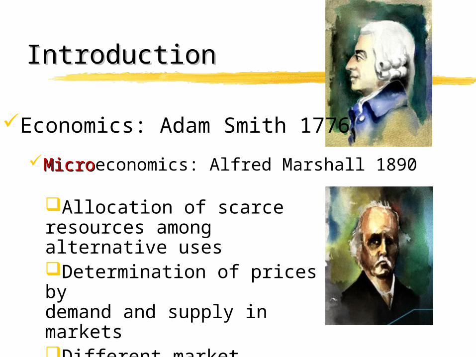
IntroductionIntroduction

MicroMicroeconomics: Alfred Marshall 1890

Economics: Adam Smith 1776

Allocation of scarce resources among alternative usesDetermination of prices by demand and supply in marketsDifferent market structures

Competition, oligopoly, monopoly

MacroeconomicsMacroeconomics

John Maynard Keynes 1936One of the chief architects of the IMF

Structure and functioning of national and international economy

Determination of national income, economic growth, unemployment, inflation, exchange rates, external debt, etc.

Grew out of the Great Depression 1929-39Microeconomics not well suited to deal with

macroeconomic problemsmacroeconomic problems

Microeconomics in actionMicroeconomics in action

Price

Quantity

Supply

Demand

P*

Q*

Equilibrium

Excess demandExcess demand

Price

Quantity

Supply

DemandExcess demand

EquilibriumProducers have powerProducers have power

Why? Consumers Why? Consumers

cannot buy all they cannot buy all they

wantwant

Excess supplyExcess supply

Price

Quantity

Supply

Demand

Excess supply

EquilibriumConsumer is kingConsumer is king

Why? Producers Why? Producers

cannot sell all they cannot sell all they

wantwant

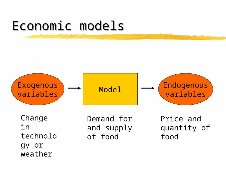
Economic modelsEconomic models

Exogenousvariables

Endogenousvariables

Model

Change in technology or weather

Demand for and supply of food

Price and quantity of food

Application to agricultureApplication to agriculture

Price

Quantity

Supply (elastic)

Demand (inelastic)

Equilibrium

Application to agricultureApplication to agriculture

Price

Quantity

Supply (elastic)

Demand (inelastic)

Income of farmers

Application to agricultureApplication to agriculture

Price

Quantity

Supply before

Demand (inelastic)

Supply after

Technological progressTechnological progressA

B

Application to agricultureApplication to agriculture

Price

Quantity

Supply before

Demand (inelastic)

Supply after

A

B

Technological progressTechnological progress

Income of farmers after Income of farmers after technical changetechnical change

The farm problemThe farm problem

No coincidence that agriculture has economic problems all over the the world

Technological progress lowers production costs and prices without inducing a significant increase in food consumptionbecause food demand is constrained by

people’s biological need for a fixed number of calories per day

Therefore, farm incomes fall!

Computers: Another storyComputers: Another story

Price

Quantity

Supply

Demand (elastic)

Computers: Another storyComputers: Another story

Price

Quantity

Supply before

Demand (elastic)

Supply after

A

B

Technological progress

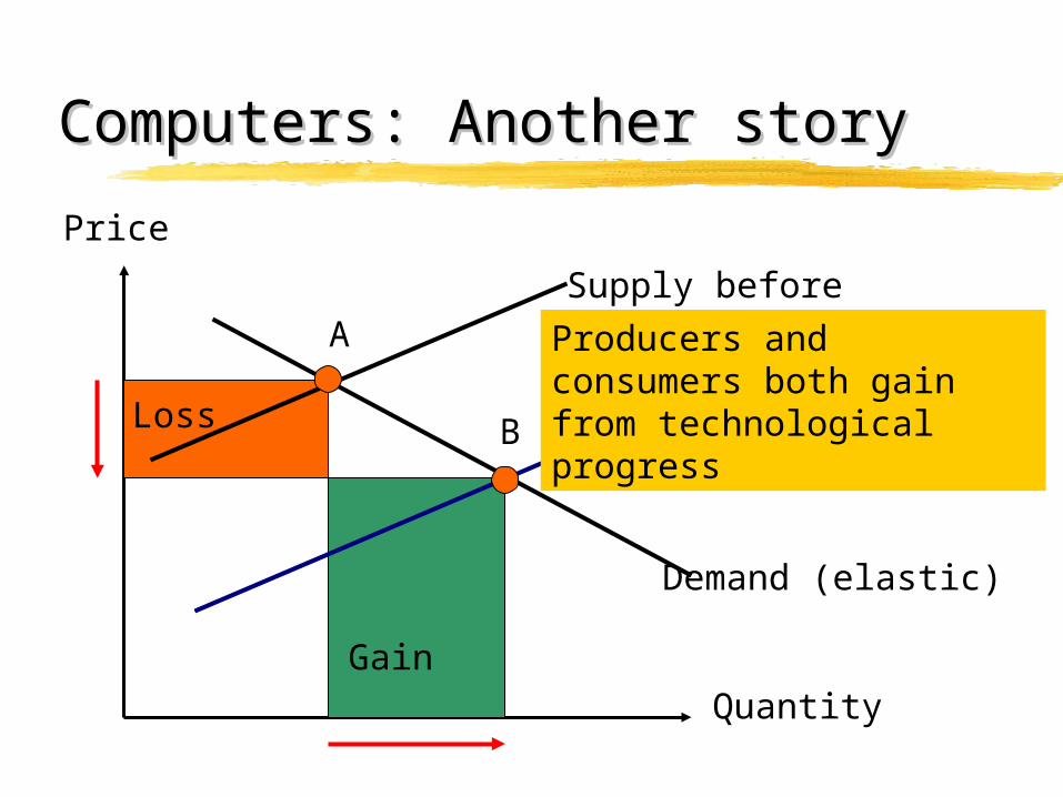
Computers: Another storyComputers: Another story

Price

Quantity

Supply before

Demand (elastic)

Supply after

A

BLoss

Gain

Producers and consumers both gain from technological progress

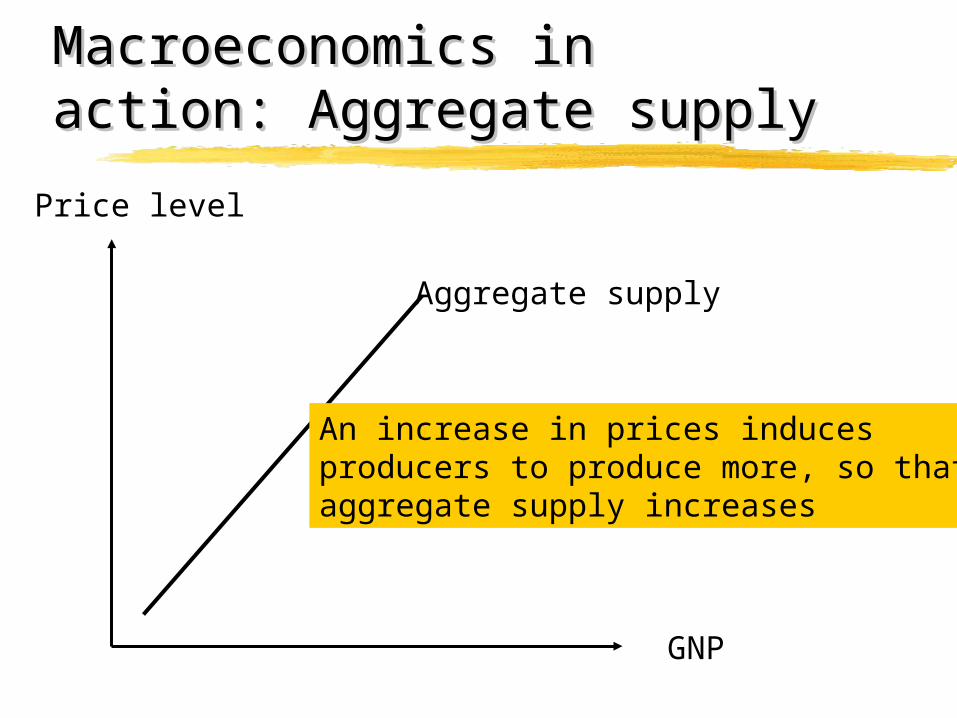
Macroeconomics in action: Macroeconomics in action: Aggregate supplyAggregate supply

Price level

GNP

Aggregate supply

An increase in prices inducesproducers to produce more, so thataggregate supply increases

Aggregate demandAggregate demand

Price level

GNP

Aggregate demand

An increase in prices inducesconsumers to buy less, so thataggregate demand decreases

Macroeconomic equilibriumMacroeconomic equilibrium

Price level

GNP

Aggregate supply

Aggregate demand

P*

Y*

Equilibrium

Excess demandExcess demand

Price level

GNP

Aggregate supply

Aggregate demand

Equilibrium

Excess demanddrives prices up, as in Eastern Europe in the 1990s

Excess demand

Excess supplyExcess supply

Price level

GNP

Aggregate supply

Aggregate demand

Equilibrium

Excess supplydrives prices down, as in America in the 1930s

Excess supply

Experiment: Export boomExperiment: Export boom

Price level

GNP

AS

AD

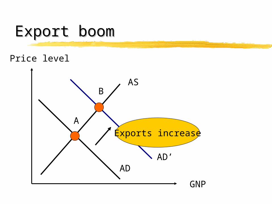
Export boomExport boom

Price level

GNP

AS

ADAD’

A

B

Exports increase

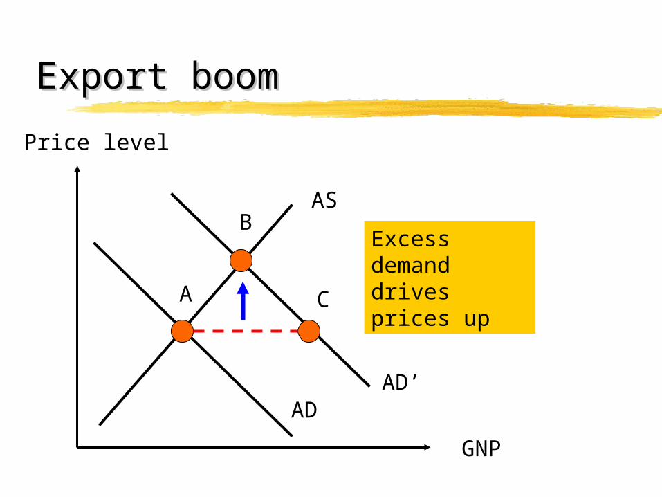
Export boomExport boom

Price level

GNP

AS

AD

Excess demanddrives prices up

AD’

A

B

C

Export boomExport boom

Price level

GNP

AS

ADAD’

A

BAs the price level rises, so does GNP along the upward-sloping AS curve

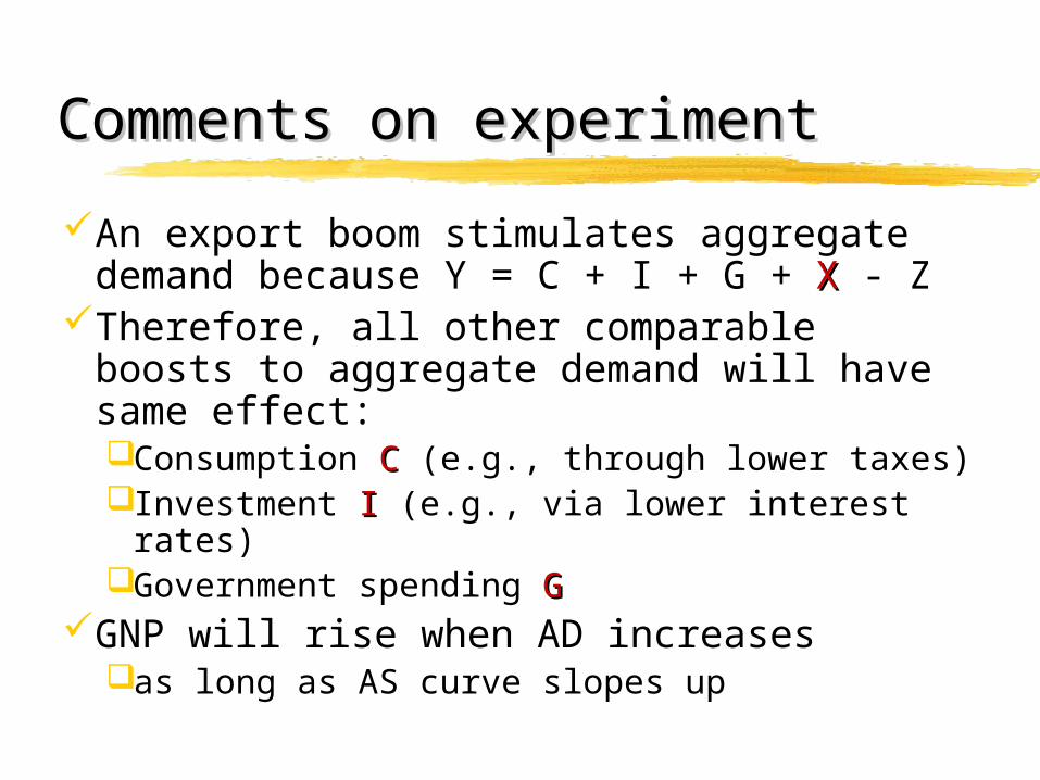
Comments on experimentComments on experiment

An export boom stimulates aggregate demand because Y = C + I + G + XX - Z

Therefore, all other comparable boosts to aggregate demand will have same effect:Consumption CC (e.g., through lower taxes)Investment II (e.g., via lower interest rates)Government spending GG

GNP will rise when AD increases as long as AS curve slopes up

An interpretationAn interpretation

Exogenousvariables

Endogenousvariables

Model

Export boom orinvestment boom

Aggregate demand and supply

Price level and GNP

Economic policyEconomic policy

Economic policy instrumentsExogenous variables

Fiscal policyFiscal policy: Government spending, taxesMonetary policyMonetary policy: Money, credit, interest ratesExchange rate policyExchange rate policy: Exchange rate (if fixed)

Economic objectives or targetsEndogenous variables

GNP level or growthPrice level or inflationEmployment, unemploymentBOP, exchange rate (if flexible), external debt

Aims of economic policyAims of economic policy

Apply policy instruments to attain given economic objectives

E.g., by conducting monetary and fiscal policy in order to strengthen the BOPKey to financial programmingfinancial programming

Not only crisis management in short runAlso, important to conduct policy so as

to foster rapid, sustainable economic growthKey to economic and social prosperity

Macroeconomic adjustment Macroeconomic adjustment and structural reformand structural reform

Begin with aggregate demandaggregate demandShow how it depends on G, t, M, e

Then add aggregate supplyaggregate supplyShow how it depends on structural

reformsThen add balance of paymentsbalance of paymentsThen make policy experiments

Assess the effects of policy measures on macroeconomic outcomes

Aggregate demandAggregate demand

Y = C + I + G + X – ZC = c(Y-T) = (1-s)(1-t)Y

Where s = saving rate and t = tax rateI = k(M/P)

Through r (real interest rate) G is exogenousX = aY* – bQZ = mY + cQ

Where Q = eP/P* (real exchange rate)

aa and mm reflect income elasticities

bb and cc reflect price elasticities

ee represents represents

foreign currency foreign currency

content of content of

domestic domestic

currencycurrency

Aggregate demandAggregate demand

Y = (1-s)(1-t)Y + kk(M/P) + G + [aY* – b(eP/P*)] – [mY + c(eP/P*)]Which means:

Y = F(P; M, G, t, e; Y*, P*) - + + - - + +

Aggregate demand schedule slopes Aggregate demand schedule slopes downdownVia real balances and the real exchange ratereal exchange rate

... and shifts in response to changes in exogenous variables, including policy

Domestic Domestic creditcredit

AD schedule slopes down

Monetary expansion shifts AD schedule right

Devaluation shifts AD schedule right

Aggregate supplyAggregate supplyY = F(N) – aggregate production functionN = N(W/P)

Labor demand varies inversely with real wages

Y = F(W/P) – or, equivalently,Y = F(P; W)

+ -

Aggregate supply schedule slopes upAggregate supply schedule slopes upThrough real wagesreal wages

... and shifts in response to changes in exogenous variables, including wages

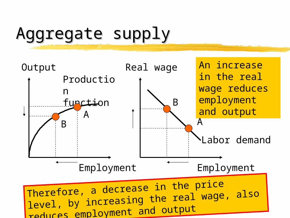
Aggregate supplyAggregate supply

Output

Employment

Real wage

Employment

Labor demand

Production function

An increase in the real wage reduces employment and outputA

BA

B

Therefore, a decrease in the price level, by

increasing the real wage, also reduces

employment and output

Macroeconomic equilibriumMacroeconomic equilibrium

Price level

GNP

AS

AD

M up; G up; t down; e down

W up

Monetary or fiscal expansionMonetary or fiscal expansion

Price level

GNP

AS

AD

M up; G up; t down

A

B

An increase in M or G or a decrease in t increases both Y and P

AD’

An increase in wagesAn increase in wages

Price level

GNP

AS

AD

W up

AS’

A

B

An increase in W increases P, but reduces Y

An increase in the price of imported oil has the same effect

DevaluationDevaluation

Price level

GNP

AS

AD

e down

W up

AD’

AS’

A

B

When e falls, W often also rises, so that P increases, but Y may either rise or fall Even if W stays put, AS will shift to the left as devaluation raises the price of oil and other imported inputs

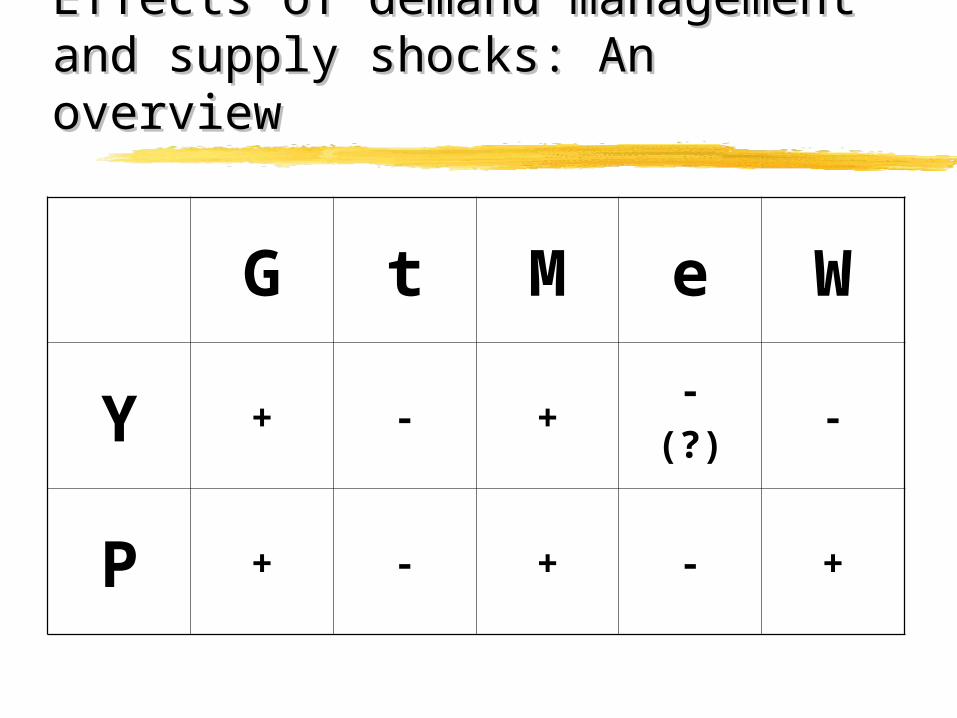
Effects of demand management Effects of demand management and supply shocks: An overviewand supply shocks: An overview

G t M e W

Y + - +-

(?)-

P + - + - +

Balance of paymentsBalance of payments

B = X – Z + FX = aY* – bQZ = mY + cQQ = eP/P*F is exogenousB = F(Y, P; e, F; Y*, P*)

- - - + + +So, to reduce deficit in the balance of

paymentsMust apply monetarymonetary or fiscal restraintfiscal restraint in order

to decrease YY or PP or decrease ee (devaluation) or increase FF (capital inflow).

Price level

GNP

AS

AD

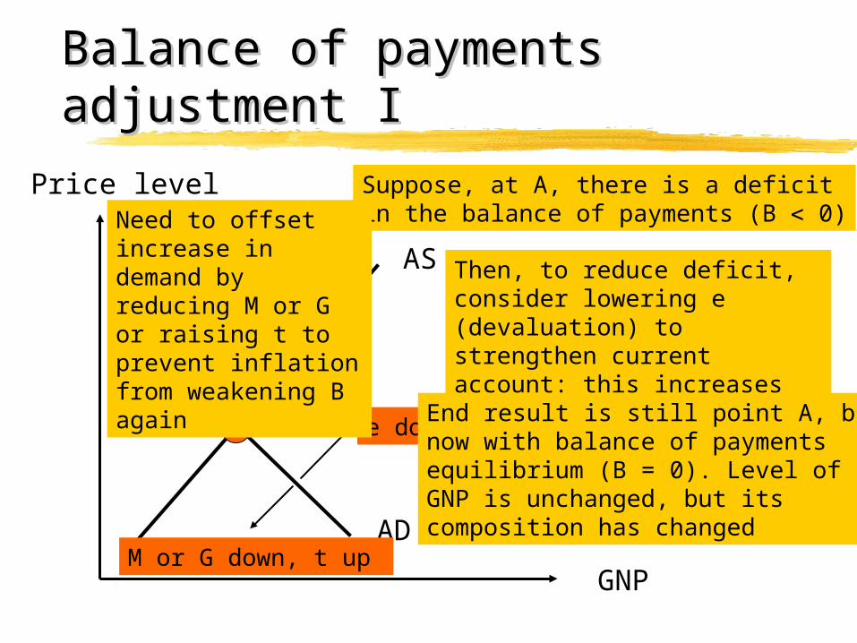
Balance of payments Balance of payments adjustment Iadjustment I

A

Suppose, at A, there is a deficitin the balance of payments (B 0)

Then, to reduce deficit, consider lowering e (devaluation) to strengthen current account: this increases demand (shifts AD right)

M or G down, t up

e downEnd result is still point A, but now with balance of paymentsequilibrium (B = 0). Level of GNP is unchanged, but its composition has changed

Need to offset increase in demand by reducing M or G or raising t to prevent inflation from weakening B again

Price level

GNP

AS

AD

Balance of payments Balance of payments adjustment IIadjustment II

A

Suppose, at A, there is a deficitin the balance of payments (B 0)

Then, to reduce deficit, considerreducing M or G or raising t toreduce demand (shift AD left)

M or G down, t up

e downEnd result is still point A, but now with balance of paymentsequilibrium (B = 0). Level of GNP is unchanged, but its composition has changed

Can offset decrease in aggregate demand by lowering e

Price level

GNP

AS

AD

Balance of payments Balance of payments adjustment IIIadjustment III

A

M or G down, t up

e down

Choice among alternative policy packages depends on initial position • If reserves are low and output is low (unemployment is high), devaluation may be advisable• If reserves are low and inflation is high, monetary and fiscal restraint may be in order• As a rule, do both at once

Price level

GNP

AS

AD

Macroeconomic adjustment Macroeconomic adjustment and structural reformand structural reform

A

Start, at A, with a deficit in the balance of payments (B 0)

To reduce deficit, consider stimulating supply (shifting AS right) as well as reducing demand

M or G down, t up

End result is point Ewith balance of paymentsequilibrium (B = 0). Level of GNP is unchanged, but its composition has changed. Bonus: Price level is lower

Stimulate supply side by liberalization, stabilization, privatization, education, etc.

E

AS’

AD’Case in point:

Marketing boards

ConclusionConclusion

The EndThe EndThe essence of financial financial

programmingprogramming is to find the right combination of monetarymonetary, fiscalfiscal, and structuralstructural policy measures that improve the balance of payments ...... without damaging other important

macroeconomic variables, including output and employment.

Theory and experience indicate that such measures are generally good for good for growthgrowth

These slides will be posted on my website: www.hi.is/~gylfason