macroalgae and phytoplankton as indicators of ecological status of
TRANSCRIPT

National Environmental Research InstituteUniversity of Aarhus . Denmark
NERI Technical Report No. 683, 2008
Macroalgae and phyto- plankton as indicators of ecological status of Danish coastal waters

[Blank page]

National Environmental Research InstituteUniversity of Aarhus . Denmark
NERI Technical Report No. 683, 2008
Macroalgae and phyto-plankton as indicators of ecological status of Danish coastal watersJacob CarstensenDorte Krause-JensenKarsten DahlPeter Henriksen

Data sheet
Series title and no.: NERI Technical Report No. 683
Title: Macroalgae and phytoplankton as indicators of ecological status of Danish coastal waters Authors: Jacob Carstensen, Dorte Krause-Jensen, Karsten Dahl & Peter Henriksen Department: Department of Marine Ecology Publisher: National Environmental Research Institute ©
University of Aarhus - Denmark URL: http://www.neri.dk
Year of publication: December 2008 Editing completed: December 2008 Referees: Henning Karup and Jens Brøgger Jensen
Financial support: Danish Environmental Protection Agency (EPA) - Water Unit
Please cite as: Carstensen, J., Krause-Jensen, D., Dahl, K. & Henriksen, P. 2008: Macroalgae and phytoplankton as indicators of ecological status of Danish coastal waters. National Environmental Research Institute, University of Aarhus. 90 pp. - NERI Technical Report No. 683. http://www.dmu.dk/Pub/FR683.pdf
Reproduction permitted provided the source is explicitly acknowledged.
Abstract: This report contributes to the development of tools that can be applied to assess the five classes of ecological status of the Water Framework Directive based on the biological quality elements phytoplankton and macroalgae. Nitrogen inputs and concentrations representing reference conditions and boundaries between the five ecological status classes were calculated from estimates of nitrogen inputs from Denmark to the Danish straits since 1900 combined with expert judgement of the general environmental conditions of Danish waters during different time periods. From these calculated nitrogen concentrations and a macroalgal model ecological status class boundaries were established for six macroalgal indicators in a number of Danish estuaries and coastal areas. Furthermore, site-specific correlations between concentrations of nitrogen and chlorophyll a were used to define reference conditions and ecological status class boundaries for the phytoplankton metric ‘mean summer concentration of chlorophyll a’ in several Danish estuaries and coastal areas. Precision of the two different chlorophyll a indica-tors ‘summer mean’ and ‘90-percentile’ was evaluated. The 90-percentile was substantially more uncertain than the mean or median indicators, particularly for small sample sizes but also for large sample sizes.
Keywords: Water Framework Directive, phytoplankton, macroalgae, indicators, models, reference condi-tion, status classification.
Layout: Anne van Acker Cover photo: Single boulder covered with brown algae at shallow waters NE of Zealand. Photo: Karsten Dahl. ISBN: 978-87-7073-060-0 ISSN (electronic): 1600-0048
Number of pages: 90
Internet version: The report is available in electronic format (pdf) at NERI's website http://www.dmu.dk/Pub/FR683.pdf

Contents
Summary 5
Sammenfatning 6
1 Introduction 7
2 Boundary values for TN concentration 8 2.1 Establishing reference TN inputs 8 2.2 Boundaries for TN concentrations 10
3 Macroalgae as indicators of water quality 18 3.1 Introduction 18 3.2 Aim 19 3.3 Methods 19 3.4 Results 30 3.5 Discussion 50 3.6 Conclusions 55
4 Assessment of ecological status using chlorophyll a 56 4.1 Boundaries for chlorophyll a 56 4.2 Comparison of boundary values for chlorophyll a and eelgrass
depth limits 62 4.3 Evaluation of the precision of the chlorophyll a indicator described as 'summer
mean' and '90th percentile' 65
5 Conclusions and recommendations 69
6 References 71
7 Appendices 75
National Environmental Research Institute
NERI technical reports

[Blank page]

Summary
During the implementation of the EU Water Framework Directive, an in-tercalibration of selected metrics of the biological quality elements was undertaken at a limited number of sites. This report describes a method for establishing ecological status classes for phytoplankton in more areas and evaluates several macroalgal indicators and their calculated indica-tor values for ecological status class boundaries.
In the first part of the report, estimates of nitrogen inputs from Denmark to the Danish straits since 1900 combined with expert judgement of the general environmental conditions of Danish waters during different time periods were used to establish nitrogen inputs representing reference conditions and boundaries between the five ecological status classes. These reference conditions and class boundaries were transformed into nitrogen concentrations in the water in several fjords and coastal locali-ties by the use of site-specific relations between nitrogen inputs and ni-trogen concentrations.
An existing macroalgal model was refined in the second part of the re-port. The model describes the following variables: i) the total algal cover, ii) the cumulative algal cover of the total algal community, opportunistic species or late-successional species, iii) the fraction of opportunistic spe-cies and iv) the number of late-successional species. All macroalgal vari-ables responded to changes in total nitrogen but also to changes in salinity which emphasises the need for setting different targets depending on sa-linity. The strongest responses to changes in nitrogen concentration and the least variability were found for the indicators 'total algal cover', 'number of late-successional species' and fraction of opportunists'. Eco-logical status class boundaries were established for all the macroalgal variables in a number of Danish estuaries and coastal areas.
A Spanish macroalgal index based on 'cover', 'proportion of opportunists' and 'species richness' was tested using Danish data. Each component of the index responded to nutrient gradients but the index needs adjust-ment of especially the scoring system in order to be applicable to Danish conditions.
In the third part of the report site-specific correlations between concen-trations of nitrogen and chlorophyll a (chla) were used to define refer-ence conditions and ecological status class boundaries for the phyto-plankton metric 'mean summer concentration of chla' in several Danish estuaries and coastal areas. The relationship between chla and nitrogen concentrations varied from site to site and reflected the bio-available fraction of total nitrogen. A relationship was demonstrated between ref-erence conditions and good-moderate boundaries for eelgrass depth limits and the corresponding values for chla.
Precision of the two different chla indicators 'summer mean' and '90-percentile was evaluated. The 90-percentile was substantially more un-certain than the mean or median indicators, particularly for small sample sizes but also for large sample sizes.
5

Sammenfatning
I forbindelse med implementeringen af det europæiske vandrammedi-rektiv blev der foretaget en interkalibrering af delelementer af de biolo-giske kvalitetselementer i et begrænset antal områder. Denne rapport be-skriver en metode til fastsættelse af miljøtilstandsklasser for kvalitets-elementet fytoplankton i yderligere en række områder samt forslag til indikatorer for makroalger med fastsættelse af miljøtilstandsklasser i en række danske områder.
På baggrund af estimater af kvælstofoverskud fra dansk landbrug tilbage til år 1900 beskriver rapportens første del fastsættelsen af tilførsler af kvælstof under referenceforhold samt under forhold, der repræsenterer perioder svarende til forskellige miljøtilstandsklasser for havmiljøet ge-nerelt. Ud fra lokale relationer mellem kvælstoftilførsler og kvælstofkon-centrationer i vandet defineres referencekoncentrationer af kvælstof samt kvælstofkoncentrationer svarende til grænseværdier mellem de fem mil-jøtilstandsklasser for en række danske fjorde og åbne kystområder.
I rapportens anden del videreudvikles en makroalgemodel, der beskri-ver i) det totale algedække, ii) det kumulative dække af hele algesam-fundet, opportunistiske arter eller kraftigere langsomt voksende arter, iii) fraktionen af opportunistiske arter og iv) antal kraftige langsomt vok-sende arter. Alle disse variable responderede på kvælstofkoncentratio-ner, men også på salinitet, hvilket understreger nødvendigheden af, at forskellige miljømål defineres for forskellige saliniteter. Det tydeligste respons på kvælstofkoncentrationer og den mindste variation fandtes for de tre indikatorer 'totale algedække', 'antal kraftige langsomt voksende arter' og 'opportunisters andel af den samlede vegetationsdækning'. Ba-seret på kvælstofkoncentrationerne svarende til grænserne mellem miljø-tilstandsklasserne er der for samtlige makroalgevariable beregnet værdier for grænserne mellem de fem miljøtilstandsklasser i en række danske fjorde og kystnære områder. Desuden blev anvendeligheden af et spansk makroalgeindeks baseret på 'algedække', 'fraktion opportunistiske arter' og 'artsrigdom' undersøgt. Det spanske indeks kræver væsentlig modifi-kation, før det kan anvendes under danske forhold.
Lokale sammenhænge mellem kvælstofkoncentrationer og koncentratio-nen af klorofyl a, der anvendes som indikator for biomasse, benyttes i rapportens tredje del til at definere afgrænsningen mellem de fem miljø-tilstandsklasser for kvalitetselementet fytoplankton i en række danske fjorde og kystnære vandområder. Data viste, at sammenhængen mellem koncentrationen af klorofyl a og kvælstofkoncentrationen varierede fra område til område og afspejlede den bio-tilgængelige fraktion af kvæl-stof. I områder, hvor der var defineret referenceforhold samt afgræns-ning mellem god og moderat tilstand for både fytoplankton og ålegræs-sets dybdegrænse, var der overensstemmelse mellem tilstandsmålene for de to kvalitetselementer. En undersøgelse af præcisionen på anvendelsen af hhv. sommermiddel eller 90-percentilen af klorofyl a som indikator demonstrerede væsentlig større usikkerhed på 90-percentilen.
6

1 Introduction
This report is part of a series of projects initiated and financed by the Danish Environmental Protection Agency (EPA) - Water Unit dealing with the implementation of the Water Framework Directive (WFD).
The WFD aims to achieve at least a good ecological status in all Euro-pean rivers, lakes and coastal waters and demands that the ecological status is quantified based primarily on biological indicators, i.e. phyto-plankton and benthic flora and fauna. The WFD demands an evaluation of which water bodies are being at risk of failing to meet the good eco-logical status in 2015.
In order to assess the ecological status, it is necessary to identify biologi-cal indicators which respond to environmental impact/anthropogenic pressures. Moreover, it is necessary to relate the levels of these indicators to biological status classes.
The aim of this project was to establish a scientific foundation which can contribute to the development of tools that can be applied to assess eco-logical status of coastal waters based on the biological quality elements phytoplankton and macroalgae. The aim included an assessment of values for the boundaries between ecological status classes with main emphasis on the boundaries between good and moderate ecological status since this boundary defines whether the ecological status is acceptable or not.
The report is divided in three chapters: a first chapter which assesses ref-erence conditions and boundary values for TN concentrations, a second chapter on macroalgae as indicators of water quality and a third chapter on phytoplankton as an indicator of water quality.
7
2 Boundary values for TN concentration
The procedure for determining reference conditions and boundary val-ues for total nitrogen (TN) was already presented and discussed in Car-stensen (2006). The procedure has been expanded with data from recent years and applied to two specific seasonal windows: 1) January-June used for relationships to summer chlorophyll (May-September) and 2) July-June used for relationships to macroalgae indicators.
2.1 Establishing reference TN inputs
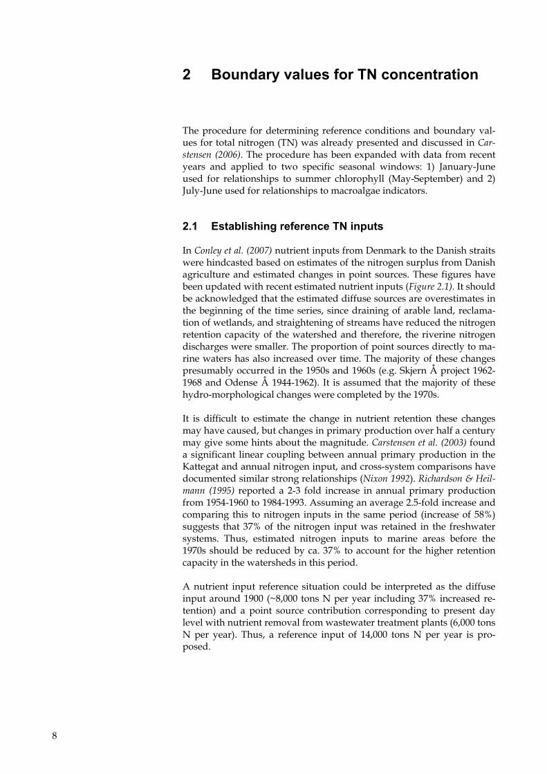
In Conley et al. (2007) nutrient inputs from Denmark to the Danish straits were hindcasted based on estimates of the nitrogen surplus from Danish agriculture and estimated changes in point sources. These figures have been updated with recent estimated nutrient inputs (Figure 2.1). It should be acknowledged that the estimated diffuse sources are overestimates in the beginning of the time series, since draining of arable land, reclama-tion of wetlands, and straightening of streams have reduced the nitrogen retention capacity of the watershed and therefore, the riverine nitrogen discharges were smaller. The proportion of point sources directly to ma-rine waters has also increased over time. The majority of these changes presumably occurred in the 1950s and 1960s (e.g. Skjern Å project 1962-1968 and Odense Å 1944-1962). It is assumed that the majority of these hydro-morphological changes were completed by the 1970s.
It is difficult to estimate the change in nutrient retention these changes may have caused, but changes in primary production over half a century may give some hints about the magnitude. Carstensen et al. (2003) found a significant linear coupling between annual primary production in the Kattegat and annual nitrogen input, and cross-system comparisons have documented similar strong relationships (Nixon 1992). Richardson & Heil-mann (1995) reported a 2-3 fold increase in annual primary production from 1954-1960 to 1984-1993. Assuming an average 2.5-fold increase and comparing this to nitrogen inputs in the same period (increase of 58%) suggests that 37% of the nitrogen input was retained in the freshwater systems. Thus, estimated nitrogen inputs to marine areas before the 1970s should be reduced by ca. 37% to account for the higher retention capacity in the watersheds in this period.
A nutrient input reference situation could be interpreted as the diffuse input around 1900 (~8,000 tons N per year including 37% increased re-tention) and a point source contribution corresponding to present day level with nutrient removal from wastewater treatment plants (6,000 tons N per year). Thus, a reference input of 14,000 tons N per year is pro-posed.
8

Figure 2.1 Long-term trends in nitrogen input from Denmark to the Danish straits. From Conley et al. (2007).
Discussions with the Danish EPA (J. Brøgger Jensen and H. Karup, pers. com.) have led to the characterisation of different ecological status classes during different periods in time. The period up to 1950 is consid-ered having a high ecological status, corresponding to a nitrogen input of about 22,000 tons N per year (including 37% increased retention). In the 1950s and early 1960s the ecological status was considered to be good, corresponding to a nitrogen input of about 32,000 tons N per year (in-cluding 37% increased retention). In the late 1960s and 1970s the situa-tion started worsening and the ecological status was considered to be moderate, corresponding to an average nitrogen input of about 73,000 tons N per year. In the 1980s the conditions were really poor (average of 91,000 tons N per year) and in certain years the status may even have been considered bad (average of 110,000 tons N per year for the 3 worst years). Nitrogen inputs in the 1990s were highly variable with an aver-age of 66,000 tons N per year, an input level similar to the 1970s and the status could be characterised as moderate. In the most recent years, the nitrogen input has been about 50,000 tons N per year, a status that may be characterised as between good and moderate status. Thus, the conse-quence of these assertions is that present day nitrogen input level charac-terises a good ecological status, assuming linearity between inputs and effects. It should be acknowledged that such proportionality assump-tions do not apply for ecological effects with a hysteretic response (type of threshold response) to changing nutrient levels. In such cases ecologi-cal status corresponds to different nutrient inputs during the eutrophica-tion development and during the eutrophication trend reversal. Bounda-ries between nutrient inputs corresponding to the 5 ecological status classes are chosen as midpoint values (Table 2.1).
9

Table 2.1 Proposed nitrogen input values corresponding to reference conditions and boundary values between ecological status classes. Nitrogen inputs are converted to a flow-weighted TN concentration using an average freshwater discharge of 8,523 km3 per year (average to the Danish straits 1942-2006). Period Boundary Nitrogen input per year Flow-weighted TN concentrationAround 1900 Reference condition 14,000 tons 117 µmol l-1 Around 1950 High → Good 27,000 tons 226 µmol l-1 Around 1965 Good → Moderate 52,500 tons 440 µmol l-1 Around 1980 Moderate → Poor 82,000 tons 687 µmol l-1 Worst years in the 1980s Poor → Bad 100,500 tons 842 µmol l-1
2.2 Boundaries for TN concentrations
A total of 39 sites were selected from the National Marine Database (MADS) that had sufficient TN data for estimating relationships to TN inputs. The sites included all areas defined within the Danish National Aquatic Monitoring and Assessment Program (DNAMAP) as well as a few additional sites that were part of regional monitoring programs. Time series of nitrogen input to the Danish straits were compiled and used to establish relationship for TN concentrations at sites connected to the Danish straits and sites located on the west coast of Denmark with a strong influence of local nutrient sources (Ringkøbing Fjord, Nissum Fjord, inner Wadden Sea). Coastal sites on the Jutland west coast are, however, more affected by nutrient inputs from the continental rivers discharging to the southern North Sea (mainly the rivers Elbe, Weser and Ems). For instance, the catchment area of River Elbe is more than 3 times larger than the total land area of Denmark and freshwater and nutrient discharges are more than twice as high as total Danish inputs (Gerlach 1990).
2.2.1 Salinity-TN relationships for coastal North Sea
Distinctive gradients (both north-south and east-west) in salinity and nu-trient concentrations characterise this area and any analysis of data from this area must take variations in salinity into account. Salinity levels typically range from 28 to 35 and TN concentrations from 0.2 to 1.5 µg l-1. In simple terms, the TN concentration in this area is determined from mixing of central North Sea water (salinity ~35) and riverine inputs. The TN concentration in the central North Sea is assumed constant (µ), whereas the TN gradient with respect to salinity varies between years and between months.
TNij = µ + monthi × (salinityij-35) + yearj × (salinityij-35)
This regression model was analysed using data from 1993 and onwards, since there were very few data before 1993. Both the month-specific gra-dients (p <0.0001) and the year-specific gradients (p <0.0001) were highly significant, with the strongest seasonal gradients for January-March and slowly decreasing gradients from 1993 to 2006 (Figure 2.2). The constant TN concentration at salinity 35 was estimated to be 13.18 (±0.50) µmol l-1.
10

Figure 2.2 Surface TN versus salinity for 1993-2006 (January-June) (top) and the estimated salinity gradients for different months (bottom left) and different years (bottom right).
The estimated gradients can be used for predicting the TN concentration at salinity 0, and compare these estimates to the riverine concentrations. Annual mean TN concentrations from the River Elbe measured in Ham-burg were obtained from EIONET (www.eea.eu.int) and in order to make these values more comparable to TN concentrations measured in January-June, a moving average of two years was computed. TN concen-trations in the Elbe River have generally decreased from about 400 µmol l-1 in the beginning of the 1990s to below 300 µmol l-1 in recent years, in accordance with the decreasing slopes of the TN-salinity gradients along the west coast (Figure 2.2). Consequently, there was a strong correlation between TN concentrations in the River Elbe and estimated TN concen-trations at salinity 0 using the relationships from the TN-salinity model (Figure 2.3). Only 1996 seems to deviate from the overall pattern, and 1996 was exceptional in the sense that extremely low concentrations were measured along the west coast. It should be noted that the pre-
11

dicted TN concentrations from the model are, on average, 27.8 µmol l-1 (±8.3) lower than measured concentration in the river, indicating a TN sink in the German Bight.
Figure 2.3 Mean annual TN concentrations in River Elbe compared to estimated TN concentrations based on the salinity-TN regression model. Data from 1996 were not in-cluded in the regression.
Assuming that the land use, and presumably nitrogen loss also, in the catchment areas of River Elbe and other contributing rivers is similar to the land use in Denmark, equivalent TN concentrations calculated from TN inputs to the Danish straits in an average freshwater discharge year (Table 2.1) minus an average TN sink of 27.8 µmol l-1 were employed as end-point members. Reference conditions and boundaries between eco-logical status classes are therefore found as salinity-dependent lines starting at 13.18 µmol l-1 for salinity 35 and intersecting 0 salinity at 80, 189, 403, 650, and 805 µmol l-1 (Table 2.2) for reference conditions, H-G boundary, G-M boundary, M-P boundary, and P-B boundary, respec-tively. Such reference conditions and boundaries were found for 4 sites along the west-coast of Jutland using average salinities characteristic for each site (Table 2.2). The uncertainty associated with these estimates de-rives from the estimated TN level at salinity 35 and the TN sink, since the TN concentrations at salinity 0 are fixed values. The values in Table 2.2 will be used for deriving reference condition and boundary values for Nissum Fjord, Ringkøbing Fjord and the inner Wadden Sea.
Table 2.2 Suggested reference conditions and boundary values for TN concentration (µmol l-1) normalised to standard salinity of 33 for Hirtshals, 31.7 for the coastal area off Nissum Fjord, 31.4 for the coastal area off Ringkøbing Fjord, and 30.4 for outer Wadden Sea. Intercalibration site Ref. cond. H-G G-M M-P P-B Hirtshals 17.0 (±0.7) 23.2 (±0.7) 35.5 (±0.7) 49.6 (±0.7) 58.4 (±0.7) Coast off Nissum Fjord 19.5 (±0.9) 29.8 (±0.9) 49.9 (±0.9) 73.2 (±0.9) 87.8 (±0.9) Coast off Ringkøbing Fjord 20.1 (±1.0) 31.3 (±1.0) 53.3 (±1.0) 78.7 (±1.0) 94.6 (±1.0) Outer Wadden Sea 22.0 (±1.2) 36.3 (±1.2) 64.4 (±1.2) 96.9 (±1.2) 117.3 (±1.2)
12

2.2.2 Nitrogen input-TN relationships for estuarine and coastal sites
Salinity gradients are less pronounced in Danish estuaries and coastal sites, although there are differences between stations within these sites, but salinity variations at specific monitoring stations are generally small. Data from 39 different sites were selected and for each of these sites year-ly TN means for January-June (for chlorophyll relationships) and July-June (for macroalgae relationships) were calculated, taking stations-spe-cific and month of sampling variations into account. TN means based on few observations and with a relative standard error of more than 15% were discarded.
To establish relationships between nitrogen input from land and TN concentrations, 39 site-specific relationships between nitrogen input and TN concentrations were found (Figure 2.4). Out of the 39 sites, 33 sites had a significant relationship (p <0.05) between TN level and nitrogen input from land. The 6 sites that did not have a significant relationship were Bornholm W, Dybsø Fjord, Fakse Bay, Hjelm Bay, Karrebæksminde Bay, and Præstø Fjord, i.e. sites that are not strongly affected by local fluvial inputs.
The regressions had different slopes but most of the regression lines ap-peared to have the same intercept (Figure 2.5). The common intercept for most of the sites corresponded to the intercept obtained from open-water stations in the Danish straits (15.46±0.88 µmol l-1). The sites with inter-cepts that deviated most from this value were Nissum Fjord and Ring-købing Fjord, both sluice controlled estuaries exchanging with the North Sea and Mariager Fjord, which is the only true Danish fjord having a sill and high retention time. For all sites, except those on the west coast, the intercept was fixed to the open-water value of 15.46 µmol l-1 and site-specific slopes were estimated. The assumption underlying this analysis is that all sites will eventually have a TN concentration of about 15.46 µmol l-1 if nitrogen inputs are completely blocked. For inner Wadden Sea, Ringkøbing Fjord and Nissum Fjord the intercept was set to the boundary value between high and good (Table 2.3) corresponding to 36.3 µmol l-1, 31.3 µmol l-1, 29.8 µmol l-1 for these sites, respectively.
13

Figure 2.4 Regression lines obtained from 39 different sites covering TN mean levels (January-June) in estuaries and coastal areas in Denmark. Nitrogen input to the Danish straits cover July to June. The regression line for open-water stations in the Danish straits is highlighted (bold, green). Solid lines are significant relationships (p <0.05) and dashed lines are insignificant relationships. Relationships for TN mean concentrations (July-June) are similar but not shown.
Figure 2.5 Estimated intercept values for 39 different sites and 95% confidence intervals for the estimate. Estimates have been sorted by increasing intercepts.
The simplified regression model with a common intercept of 15.46 µmol l-1 gave site-specific slopes that varied substantially (Figure 2.6). All open coastal sites (16 lowest slopes) generally have the same slope indicating that TN levels do not deviate substantially from each other. For estuaries and enclosed coastal areas, starting with Åbenrå Fjord, Vejle Fjord and
14

Flensborg Fjord on the ranked scale, the response to nitrogen input is about 2-3 times larger than for open coastal sites. The largest response to nitrogen input is observed for inner Odense Fjord, Nissum Fjord and Randers Fjord, sites strongly affected by riverine inputs. Overall the ranking of the sites by their slopes corresponds well to the expected in-fluence from land-based nitrogen discharges.
Figure 2.6 Estimated site-specific slopes in TN-nitrogen input relations and 95% confidence intervals for the estimate. Esti-mates have been sorted by increasing slopes.
For the 39 different water bodies, reference conditions and boundary val-ues between ecological status classes were predicted from the regression model using fixed intercepts and site-specific slopes (Table 2.3). The un-certainty of these estimates includes a variance contribution from both the slope and the estimated common intercept of 15.46 µmol l-1 (±0.88).
For the TN concentrations used in the macroalgae calculations the pro-cedure is similar with the exception that TN annual means represent an entire year (July-June). Given this, we found values (Table 2.4) that were slightly lower than those used for chlorophyll due to generally lower TN levels in July-December compared to January-June.
15

Table 2.3 Suggested reference conditions and boundary values for TN concentration (µmol l-1) for January-June computed from corresponding values of nitrogen by means of the regression model with site-specific slopes. These values were used for calculating corresponding reference conditions and boundary values for chlorophyll a. Locality Ref. cond. H-G G-M M-P P-B Archipelago of southern Fyn 17.8 (+/-1.1) 19.9 (+/-1.4) 24.1 (+/-2.1) 28.9 (+/-3.1) 32.0 (+/-3.8) Augustenborg Fjord 20.7 (+/-1.9) 25,4 (+/-3.3) 34,8 (+/-6.1) 45.7 (+/-9.5) 52.5 (+/-12.0) Bornholm West 16.4 (+/-1.2) 17,2 (+/-1.7) 18,8 (+/-2.8) 20.7 (+/-4.1) 21.9 (+/-5.0) Dybsø Fjord 23.0 (+/-2.8) 30.0 (+/-5.2) 43.6 (+/-9.9) 59.4 (+/-15.0) 69.3 (+/-19.0) Fakse Bay 16.6 (+/-1.5) 17.6 (+/-2.4) 19.5 (+/-4.4) 21.8 (+/-6.7) 23.2 (+/-8.2) Flensborg Fjord 19.4 (+/-1.1) 23.0 (+/-1.4) 30.2 (+/-2.2) 38.4 (+/-3.2) 43.6 (+/-3.8) Fyns Hoved / Great Belt 16.7 (+/-1.1) 17.8 (+/-1.2) 20.0 (+/-1.6) 22.6 (+/-2.3) 24.2 (+/-2.7) Hevring Bay 17.1 (+/-1.2) 18.7 (+/-1.7) 21.7 (+/-2.8) 25.1 (+/-4.2) 27.3 (+/-5.2) Hjelm Bay 16.7 (+/-1.7) 17.7 (+/-2.7) 19.9 (+/-5.0) 22.3 (+/-7.8) 23.9 (+/-9.5) Horsens Fjord 21.5 (+/-1.2) 27.0 (+/-1.5) 37.9 (+/-2.5) 50.5 (+/-3.7) 58.4 (+/-4.5) Isefjord 19.8 (+/-1.1) 23.7 (+/-1.3) 31.4 (+/-2.0) 40.4 (+/-2.9) 46.0 (+/-3.5) Kalundborg Fjord 17.3 (+/-1.1) 19.1 (+/-1.4) 22.4 (+/-2.1) 26.3 (+/-3.1) 28.8 (+/-3.7) Karrebæksminde Bay 17.4 (+/-1.9) 19.2 (+/-3.3) 22.8 (+/-6.1) 26.8 (+/-9.5) 29.4 (+/-12.0) Kertinge Nor 22.1 (+/-1.2) 28.2 (+/-1.6) 40.2 (+/-2.5) 54.0 (+/-3.8) 62.7 (+/-4.6) Køge Bay 17.0 (+/-1.1) 18.4 (+/-1.4) 21.1 (+/-2.1) 24.3 (+/-3.1) 26.2 (+/-3.7) The Little Belt 16.9 (+/-1.0) 18.3 (+/-1.2) 20.9 (+/-1.6) 23.9 (+/-2.1) 25.8 (+/-2.5) Limfjorden 35.7 (+/-2.1) 54.5 (+/-3.8) 91.4 (+/-7.2) 134.0 (+/-11.0) 161.0 (+/-14.0)Limfjord East 26.3 (+/-1.1) 36.3 (+/-1.4) 55.9 (+/-2.3) 78.6 (+/-3.3) 92.8 (+/-4.0) Limfjorden S of Mors 23.6 (+/-1.2) 31.1 (+/-1.7) 45.9 (+/-2.8) 62.9 (+/-4.2) 73.6 (+/-5.1) Løgstør Bredning 26.0 (+/-1.2) 35.8 (+/-1.7) 54.9 (+/-2.9) 77.1 (+/-4.4) 91.0 (+/-5.4) Nissum Bredning 22.5 (+/-1.2) 28.9 (+/-1.6) 41.6 (+/-2.7) 56.3 (+/-4.1) 65.5 (+/-4.9) Nissum Fjord 41.7 (+/-1.1) 66.0 (+/-1.5) 114.0 (+/-2.3) 169.0 (+/-3.4) 204.0 (+/-4.2) North of Zealand 16.5 (+/-1.1) 17.5 (+/-1.3) 19.3 (+/-2.0) 21.5 (+/-2.8) 22.8 (+/-3.4) Northern Kattegat 16.9 (+/-1.1) 18.2 (+/-1.5) 20.7 (+/-2.4) 23.6 (+/-3.5) 25.5 (+/-4.2) Odense Fjord inner 47.2 (+/-1.4) 76.6 (+/-2.2) 134.0 (+/-4.0) 201.0 (+/-6.1) 243.0 (+/-7.5) Odense Fjord outer 26.4 (+/-1.2) 36.4 (+/-1.5) 56.2 (+/-2.4) 79.1 (+/-3.6) 93.5 (+/-4.4) Open waters 16.7 (+/-1.0) 17.7 (+/-1.1) 19.9 (+/-1.2) 22.3 (+/-1.5) 23.8 (+/-1.7) Præstø Fjord 23.7 (+/-1.7) 31.3 (+/-2.9) 46.2 (+/-5.4) 63.5 (+/-8.3) 74.4 (+/-10.0) Randers Fjord 37.4 (+/-1.3) 57.7 (+/-1.8) 97.6 (+/-3.0) 144.0 (+/-4.6) 173.0 (+/-5.5) Ringkøbing Fjord after 1996 33.5 (+/-1.1) 50.2 (+/-1.4) 82.9 (+/-2.1) 121.0 (+/-3.0) 145.0 (+/-3.6) Ringkøbing Fjord before 1996 34.6 (+/-1.3) 52.3 (+/-1.8) 87.1 (+/-3.2) 127.0 (+/-4.8) 153.0 (+/-5.8) Roskilde Fjord 25.6 (+/-1.1) 35.0 (+/-1.3) 53.5 (+/-1.8) 74.8 (+/-2.6) 88.2 (+/-3.1) Sejerø Bay 16.9 (+/-1.3) 18.2 (+/-1.9) 20.7 (+/-3.2) 23.6 (+/-4.9) 25.4 (+/-5.9) Skive Fjord / Lovns Bredning 28.9 (+/-1.0) 41.3 (+/-1.1) 65.7 (+/-1.4) 93.9 (+/-1.8) 112.0 (+/-2.1) Vejle Fjord 19.4 (+/-1.1) 23.0 (+/-1.5) 30.1 (+/-2.4) 38.2 (+/-3.5) 43.4 (+/-4.2) Wadden Sea inner part 24.0 (+/-1.1) 31.8 (+/-1.4) 47.3 (+/-2.1) 65.1 (+/-3.1) 76.3 (+/-3.7) The Sound North 16.4 (+/-1.2) 17.3 (+/-1.6) 19.0 (+/-2.6) 20.9 (+/-3.9) 22.1 (+/-4.7) Åbenrå Fjord 18.7 (+/-1.4) 21.6 (+/-2.1) 27.4 (+/-3.8) 34.2 (+/-5.7) 38.4 (+/-7.0) Århus Bay 16.4 (+/-1.1) 17.2 (+/-1.2) 18.8 (+/-1.7) 20.7 (+/-2.3) 21.9 (+/-2.8)
16

Table 2.4 Suggested reference conditions and boundary values for TN concentration (µmol l-1) for July-June computed from corresponding values of nitrogen by means of the regression model with site-specific slopes. These values were used for calcu-lating corresponding reference conditions and boundary values for macroalgae.
Locality Ref. cond. H-G G-M M-P P-B Open coasts Bornholm West 16.6 (+/-1.1) 17.6 (+/-1.4) 19.6 (+/-2.1) 21.9 (+/-3.1) 23.4 (+/-3.8) Bornholm East 16.2 (+/-1.1) 16.8 (+/-1.3) 18.0 (+/-2) 19.4 (+/-2.9) 20.3 (+/-3.5) Endelave 17.4 (+/-1.4) 19.1 (+/-2.2) 22.4 (+/-3.9) 26.3 (+/-6.0) 28.8 (+/-7.4) Hesselø 16.0 (+/-1.6) 16.4 (+/-2.7) 17.3 (+/-5.0) 18.4 (+/-7.6) 19.0 (+/-9.3) Hevring Bay 16.7 (+/-1.1) 17.8 (+/-1.3) 20.0 (+/-1.9) 22.5 (+/-2.6) 24.1 (+/-3.2) Hjelm Bay 16.1 (+/-1.2) 16.7 (+/-1.5) 17.8 (+/-2.5) 19.0 (+/-3.7) 19.8 (+/-4.5) Karrebæksminde Bay 17.0 (+/-1.3) 18.4 (+/-1.9) 21.1 (+/-3.3) 24.3 (+/-5.0) 26.3 (+/-6.1) Køge Bay 17.2 (+/-1.1) 18.9 (+/-1.3) 22.0 (+/-1.9) 25.7 (+/-2.7) 28.0 (+/-3.2) The Little Belt coast 16.8 (+/-1.0) 18.0 (+/-1.0) 20.4 (+/-1.1) 23.2 (+/-1.3) 24.9 (+/-1.4) Nivå Bay 16.4 (+/-1.1) 17.2 (+/-1.4) 18.8 (+/-2.2) 20.6 (+/-3.2) 21.8 (+/-3.9) North of Zealand 16.0 (+/-1.1) 16.4 (+/-1.3) 17.2 (+/-1.8) 18.1 (+/-2.6) 18.7 (+/-3.1) Northern Belt Sea coast 16.5 (+/-1.1) 17.5 (+/-1.3) 19.4 (+/-2.0) 21.6 (+/-2.9) 23.0 (+/-3.5) Sejerø Bay 16.8 (+/-1.1) 18.0 (+/-1.3) 20.3 (+/-2.0) 23.1 (+/-2.9) 24.8 (+/-3.5) Archipelago of southern Fyn 17.4 (+/-1.1) 19.1 (+/-1.3) 22.5 (+/-1.9) 26.5 (+/-2.7) 28.9 (+/-3.2) The Sound 16.4 (+/-1) 17.3 (+/-1.1) 19.0 (+/-1.3) 20.9 (+/-1.6) 22.1 (+/-1.8) Århus Bay 16.2 (+/-1) 16.8 (+/-1.1) 18.0 (+/-1.4) 19.5 (+/-1.8) 20.4 (+/-2.0) Inner fjords Augustenborg Fjord 19.8 (+/-1.2) 23.7 (+/-1.6) 31.5 (+/-2.6) 40.4 (+/-3.9) 46.0 (+/-4.7) Dybsø Fjord 20.3 (+/-1.5) 24.7 (+/-2.3) 33.4 (+/-4.1) 43.4 (+/-6.3) 49.7 (+/-7.7) Flensborg Fjord 20.5 (+/-1.1) 25.1 (+/-1.4) 34.2 (+/-2.1) 44.7 (+/-3.0) 51.2 (+/-3.6) Genner Fjord 18.9 (+/-1.3) 22.0 (+/-1.9) 28.1 (+/-3.2) 35.2 (+/-4.8) 39.6 (+/-5.9) Horsens Fjord 21.6 (+/-1.1) 27.2 (+/-1.5) 38.2 (+/-2.4) 51.0 (+/-3.5) 59.0 (+/-4.2) Isefjord 21.2 (+/-1.2) 26.6 (+/-1.6) 37.0 (+/-2.6) 49.1 (+/-3.9) 56.6 (+/-4.8) Kalundborg Fjord 17.4 (+/-1.1) 19.2 (+/-1.4) 22.6 (+/-2.1) 26.6 (+/-3.0) 29.1 (+/-3.6) Karrebæk Fjord 31.1 (+/-2.0) 45.5 (+/-3.4) 73.9 (+/-6.5) 106.6 (+/-10.1) 127.2 (+/-12.3) Kertinge Nor 21.7 (+/-1.1) 27.4 (+/-1.3) 38.6 (+/-1.8) 51.6 (+/-2.5) 59.7 (+/-3.0) Kolding Fjord 22.3 (+/-1.4) 28.6 (+/-2.1) 41.0 (+/-3.7) 55.3 (+/-5.7) 64.2 (+/-6.9) Korsør Nor 21.4 (+/-1.3) 26.8 (+/-1.8) 37.6 (+/-3.2) 50.0 (+/-4.8) 57.7 (+/-5.8) Limfjorden NW of Mors 23.9 (+/-1.1) 31.7 (+/-1.3) 47.0 (+/-1.9) 64.7 (+/-2.7) 75.8 (+/-3.2) Limfjorden S of Mors 22.1 (+/-1.0) 28.2 (+/-1.2) 40.1 (+/-1.5) 53.9 (+/-2.0) 62.6 (+/-2.4) Limfjorden W of Mors 22.1 (+/-1.1) 28.2 (+/-1.3) 40.1 (+/-1.9) 53.9 (+/-2.8) 62.6 (+/-3.3) Nakkebølle Fjord 26.0 (+/-3.7) 35.8 (+/-6.9) 55.0 (+/-13.3) 77.2 (+/-20.7) 91.1 (+/-25.3) Odense Fjord 37.7 (+/-1.2) 58.4 (+/-1.5) 98.9 (+/-2.4) 145.7 (+/-3.6) 175.1 (+/-4.4) Præstø Fjord 21.2 (+/-1.2) 26.4 (+/-1.6) 36.8 (+/-2.7) 48.7 (+/-4.1) 56.2 (+/-5.0) Roskilde Fjord 29.3 (+/-1.1) 42.1 (+/-1.2) 67.2 (+/-1.6) 96.3 (+/-2.2) 114.5 (+/-2.6) Skive Fjord 27.5 (+/-1.0) 38.5 (+/-1.1) 60.3 (+/-1.3) 85.5 (+/-1.7) 101.3 (+/-1.9) Vejle Fjord 18.8 (+/-1.1) 21.8 (+/-1.4) 27.8 (+/-2.1) 34.6 (+/-3.1) 39.0 (+/-3.8) Eastern Limfjord 24.6 (+/-1.1) 33.1 (+/-1.2) 49.8 (+/-1.6) 69.0 (+/-2.3) 81.1 (+/-2.7) Åbenrå Fjord 18.8 (+/-1.1) 21.9 (+/-1.4) 27.9 (+/-2.3) 34.9 (+/-3.3) 39.3 (+/-4.0) Outer fjords Flensborg Fjord 17.5 (+/-1.2) 19.3 (+/-1.6) 23.0 (+/-2.7) 27.2 (+/-4.0) 29.8 (+/-4.9) Horsens Fjord 19.1 (+/-1.1) 22.4 (+/-1.5) 28.9 (+/-2.3) 36.5 (+/-3.4) 41.2 (+/-4.1) Isefjord 18.8 (+/-1.1) 21.9 (+/-1.3) 28.0 (+/-1.8) 35.0 (+/-2.6) 39.4 (+/-3.1) Kalundborg Fjord 17.1 (+/-1.1) 18.5 (+/-1.4) 21.4 (+/-2.1) 24.7 (+/-3.1) 26.7 (+/-3.7) Løgstør Bredning 23.6 (+/-1.1) 31.1 (+/-1.2) 45.8 (+/-1.7) 62.9 (+/-2.4) 73.6 (+/-2.9) Nissum Bredning 21.4 (+/-1.1) 26.9 (+/-1.2) 37.7 (+/-1.7) 50.1 (+/-2.4) 57.9 (+/-2.8) Odense Fjord 23.9 (+/-1.1) 31.7 (+/-1.2) 46.9 (+/-1.7) 64.6 (+/-2.3) 75.7 (+/-2.8) Roskilde Fjord 20.5 (+/-1.0) 25.1 (+/-1.2) 34.2 (+/-1.5) 44.6 (+/-2.1) 51.2 (+/-2.4) Skive Fjord 24.0 (+/-1.1) 31.9 (+/-1.2) 47.3 (+/-1.7) 65.2 (+/-2.3) 76.5 (+/-2.8) Venø Bay 22.4 (+/-1.1) 28.8 (+/-1.5) 41.3 (+/-2.3) 55.8 (+/-3.4) 64.9 (+/-4.1)
17
3 Macroalgae as indicators of water quality
3.1 Introduction
Eutrophication is a major threat to submerged plant communities. In-creased nutrient richness stimulates the growth of planktonic algae and thereby reduces water clarity and shades the benthic vegetation (e.g. Nielsen et al. 2002a). The shading effect may be further accentuated by epiphytic algae which also tend to proliferate under eutrophic conditions (Borum 1985). Lack of light reduces the depth penetration of benthic vegetation (Duarte 1991; Nielsen et al. 2002b) and also reduces vegetation abundance in the deeper, light limited waters (Duarte 1991; Dahl & Car-stensen 2008).
Opportunistic and perennial macroalgal species may respond differently to changes in nutrient and light levels. Nutrient enrichment tends to stimulate the growth of opportunistic algae which then shade the peren-nial species (Littler & Littler 1980; Steneck & Dethiers 1994; Duarte 1995; Pedersen 1995). The abundance of opportunistic algae is therefore likely to increase at the expense of perennial algae as a function of increased nutrient input. Moreover, the number of algal species may decline along a nutrient gradient (Middelboe et al. 1997).
In our previous work for the Danish EPA we tested the response of Dan-ish coastal macroalgal communities to eutrophication and found that it to some extent followed the patterns outlined above (Carstensen et al. 2005, Krause-Jensen et al. 2007a & b). The abundance of the macroalgal community as a whole as well as the abundance of perennial and oppor-tunistic algae at given depths decreased significantly along a eutrophica-tion gradient. By contrast, the relative abundance of opportunists did not respond to changes in nutrient level, but instead responded to changes in salinity, being largest in the most brackish areas. These results indicate that at large geographical scales the marked salinity gradient of the Danish coastal waters overrules possible effects of nutrients on the relative abundance of opportunists.
Our previous studies of the coastal Danish macroalgae thus strongly suggested that cover of the total macroalgal community and cover of perennial macroalgae are useful indicators of water quality. However, there is a need to develop these indicators to become even more sensitive to changes in water quality, to define boundaries between ecological status classes and to describe precisely how to use the indicators for as-sessing water quality according to the WFD.
For Spanish coastal waters it has been identified that not only the cover of characteristic algal species declines along a nutrient gradient, the number of the characteristic species also declines and the fraction of the total algal community made up by opportunistic algae increases along
18

the gradient. These responses have been combined into a single index, the CFR-Index (Cover, Fraction, Richness) as a descriptor of the status of the macroalgal community (Juanes et al. 2008). Whether the same index can be applied in Danish coastal waters is yet to be tested.
3.2 Aim
The overall aim of this project was to develop tools for assessing water quality of Danish coastal areas based on macroalgae.
Firstly, we aimed to improve the macroalgal cover indicators for use un-der the WFD by: • basing the models on more data sets and refining the models by
stratifying the data further, • assessing site-specific reference levels and boundary values for eco-
logical status classes, e.g. high/good and good/moderate status, • analysing sensitivity of the indicators, • testing how status assessment based on Danish algal indicators match
status assessment based on Swedish algal indicators for the Oresund region
• providing a step-by-step guidance for using the indicator to assess water quality according to the WFD.
Secondly, we aimed to evaluate whether the "Spanish index" is suitable for Danish conditions. This will done by: • testing whether the individual components of the "Spanish CFR-
index", i.e. cover, proportion of opportunists and species richness re-flect nutrient gradients in Danish coastal waters,
• analysing whether the scoring system of the Spanish CFR-index is applicable for Danish coastal waters.
3.3 Methods
3.3.1 Algal data
We used data from the Danish National Monitoring and Assessment Programme and regional monitoring activities collected by the Danish counties and stored centrally in the National Environmental Research In-stitute's (NERI's) database. Data (2665-2668 observations for the different indicators) were distributed along 1-18 sites each with a number of ob-servations along a depth gradient in each of 34 coastal areas (Table 3.1, Figure 3.1). Some of the areas were subdivided so that the data set con-tained a total of 44 areas/sub-areas. Algal data were collected during summer (May-September) of 2001, 2003 and 2005 (since our previous analyses of the coastal macroalgae, some of the data from 2001 and 2003 have been revised and, in some cases changed, by the Local Environ-mental Authorities). We chose to use data from 2001 onwards rather than the entire data set dating back to 1989 because the recent data set is more uniform and better integrated with the pelagic monitoring pro-
19

gram. Data were collected according to new common guidelines (Krause-Jensen et al. 2001), where divers visually recorded the percent cover of in-dividual erect algal species and of the total erect macroalgal community (excluding the crust-forming algae). Algal cover was estimated in per-cent of the hard substratum within 3 sub-areas of 25 m2 at specific depth in each 2-m depth interval along the depth gradients/sites.
Data sets where the summed cover of algal species constituted <80% of the estimated total algal cover were excluded, because we suspected that species registration in these data sets might be incomplete.
All species were allocated to a functional group, using the system of Steneck & Dethiers (1994, Table 3.2). The functional groups 1-3: micro-algae, filamentous algae and single-layered foliose algae are dominated by opportunistic algal species with thin thalli, fast growth rates and ephemeral life forms, while the remaining groups primarily include per-ennial species with thick, corticated, leathery or calcareous thalli and relatively slow growth rates. In the following we therefore refer to group 2, 2.5 and 3 as 'opportunistic macroalgae' while algae belonging to groups 4, 5 and 6 are considered 'late-successional algae'. Group 2.5 in-cludes species which are borderline cases between opportunists and late-successionals. We tested whether we could improve the models by in-cluding some of the algal from group 2.5 in the group of late-suc-cessionals. This was not the case, and we therefore kept the grouping as described above. Microalgae (functional group 1) and crustose algae (functional group 7) were not consistently recorded in the entire data set and were therefore excluded from analysis.
Figure 3.1 Map showing the location of sampling areas. Num-bers refer to the areas listed in Table 3.1.
Denmark
Sweden
Norway
Germany
0 50 100 km
W1
W3
W2
W4
W5
W6
M8
M9
M14
M13M1
M2
M11
M6
M5
M3
M12
M4M10
M15M7
H1
H2
H11
H6
H5
H8
H13
H7
H9
H12
H3H4
H10
20

Table 3.1 Overview of sampling areas, depth range and number of sites and observa-tions of the macroalgal variables included in the analyses. Number of observations is indicated in parentheses for the variables 'total cover' and 'cumulated cover', and except for Roskilde Fjord, the number of observations of the two variables is equal. Sampling years: 2001, 2003 and 2005. Area numbers (No.) refer to the numbers in Figure 3.1. (No.) Area Depth range (m) No. of sites (No. of obs.) Weakly exposed areas (W1) Limfjorden, Venø Bay 3-5 2 (21) (W2) Limfjorden, Mors NW 1-7 3 (92) (W3) Limfjorden, Mors W 1-5 3 (71) (W4) Limfjorden, Skive Fjord 1-7 4 (116) (W5) Roskilde Fjord 1-7 7 (106-109) (W6) Genner Fjord 1-5 1 (10) Moderately exposed areas (M1) Augustenborg Fjord 3-9 5 (52) (M2) Flensborg Fjord 3-13 11 (142) (M3) Horsens Fjord 3-7 5 (17) (M4) Isefjord 3-7 11 (61) (M5) Kalundborg Fjord 3-11 18 (157) (M6) Karrebæksminde Bay 3-9 4 (33) (M7) Køge Bay 3-9 6 (84) (M8) Limfjorden, Løgstør Broad 3-7 4 (69) (M9) Limfjorden, Nissum Broad 3-7 3 (52) (M10) Nivå Bay 3-7 2 (21) (M11) Odense Fjord 3-5 1 (18) (M12) Vejle Fjord 3-13 5 (56) (M13) Åbenrå Fjord 3-9 8 (84) (M14) Århus Bay 3-13 10 (226) (M15) The Sound 3-13 11 (196) Highly exposed areas (H1) Archipelago of southern Fyn 3-9 6 (38) (H2) Beltsea N 5-13 3 (24) (H3) Bornholm W 5-13 5 (111) (H4) Bornholm E 5-13 4 (88) (H5) Ebeltoft 5-13 7 (45) (H6) Endelave 5-13 2 (14) (H7) Great Belt 5-11 5 (60) (H8) Hesselø 5-13 1 (34) (H9) Hjelm Bay 5-13 5 (84) (H10) Kirkegrund/ Knudshoved 5-13 5 (79) (H11) The Little Belt 5-13 14 (208) (H12) Zealand N 5-13 5 (134) (H13) Sejerø Bay 5-11 10 (62) Total 196 (2665-2668)
21

Table 3.2 Overview of functional groups (Steneck & Dethiers 1994) and our grouping of late-successional and opportunistic species in the present study. *Microalgae and crustose algae are not represented in the present study and therefore not included in our grouping. Functional group Examples of algal genus Grouping in this study 1. Microalgae (single cell)* Cyanobacteria and diatoms 2. Filamentous algae (uniseriate) Cladophora, Bangia 2.5 Filamentous and thinly corticated algae Polysiphonia, Ceramium, Sphacelaria Opportunists 3. Foliose algae (single layer) Monostroma, Ulva, Porphyra Opportunists 3.5 Foliose algae (corticated) Dictyota, Padina Opportunists 4. Corticated macrophytes Chondrus, Gigartina Late-successionals 5. Leathery macrophytes Laminaria, Fucus, Halidrys Late-successionals 6. Articulated calcareous algae Corallina, Halimeda Late-successionals 7. Crustose algae* Lithothamnion, Peyssonnelia, Ralfsia
We analysed six algal variables: Total cover represented the diver es-timates of total erect macroalgal cover for each sub-sample, which repre-sented values in the range 0-100%. Cumulated cover was calculated by summing the cover values of all erect macroalgal species in each sub-sample. Cumulated cover values could surpass 100%, because algae can grow in several layers. The remaining algal variables to be analysed were related to the composition of the macroalgal community. Cumulated cover of opportunistic algae was calculated as the summed cover of all algal species belonging to functional groups 1-3, and cumulated cover of late-successional algae was calculated as the summed cover of algae be-longing to algal groups 4-6. Relative cover of opportunistic algae was fi-nally calculated by dividing the cumulated cover of opportunists by the cumulated cover of all species and therefore provided data in the range 0-100%. Finally, the number of late-successional algal species in each subsample was calculated as the total number of the species belonging to this group and having a cover of at least 1%.
All algal variables were tested for responses to physico-chemical gra-dients and, thus, for their potential as indicators of water quality ac-cording to the WFD.
3.3.2 Substratum
Composition of substratum was registered along with the collection of algal data. Divers visually recorded the total cover of suitable hard sub-stratum as well as the cover of various substratum classes: size classes of stones, sand, mud and shells. Data on cover of suitable hard substratum were extracted from the database together with each algal data set.
3.3.3 Physico-chemical variables
Spatial variations in algal variables were related to the physico-chemical variables salinity, nutrient concentration, chlorophyll concentration and Secchi depth. These data were sampled at sites situated in the vicinity of vegetation sites. The water chemistry sites were typically located cen-trally in the investigated coastal areas or sub-areas, and generally 2 or more algal sites/depth gradients were related to the same water chemistry site.
22

We assumed that mean values from the various algal sites would repre-sent the algae of a given coastal area and that the centrally located water chemistry site would represent the physical conditions and water chem-istry of the same coastal area in spite of some distance between macroal-gal and water chemistry sites.
Water chemistry data were collected by the Danish counties and stored in NERI's database. Sampling and chemical analysis were performed ac-cording to common guidelines (Andersen et al. 2004) and typically repre-sented a sampling frequency between weekly and monthly sampling.
3.3.4 Statistical analyses of algal variables
Algal model We focused the analysis exclusively on algae from the depth range where disturbance was no longer a major controlling factor for cover (see Figure 3.2). The coastward end of this depth range was estimated as the water depth with highest algal cover using non-parametric adjustment (LOESS, Cleveland 1979). This adjustment was made separately for each area and showed that the areas could be categorised in weakly exposed areas where maximum cover was located at water depths of ~1 m, mod-erately exposed areas with maximum cover at water depths of ~3 m and highly exposed areas with maximum cover at water depths of ~5 m (Car-stensen et al. 2005). As a consequence, we restricted the analysis to water depths >1 m in weakly exposed areas, >3 m in moderately exposed areas and >5 m in highly exposed areas. Only few (122) observations repre-sented water depths >13 m at 6 specific localities (Bornholm West and East, North of Zealand, Hesselø and Little Belt, Northern Belt Sea) and we therefore restricted the analysis to water depths <13 m.
Figure 3.2 Illustration of the hypothesis that algal cover in shallow water is reduced due to physical exposure while from intermediate water depth towards deeper water algal cover is re-duced in parallel to reductions in available irradiance. As a conse-quence, maximum algal cover is found at intermediate water depths and is located deeper in more exposed areas.
Algal cover was estimated as substratum-specific cover, which should imply that cover levels were independent of substratum composition at the sampling sites. A possible dependence on the amount of hard sub-stratum was tested initially using a non-parametric adjustment (LOESS, Cleveland 1979) of each of the potential algal indicators to the amount of hard substratum. This analysis led to the formulation of a model, in
23

which the relation between algal cover and hard substratum differed for levels of hard substratum of below and above 50%.
Algal data representing cumulated cover levels were ln transformed be-fore analysis. By contrast, raw values of the algal variables 'total cover' and 'fraction of opportunists' were in the range 0-100% and greater varia-tion was expected around 50% than at 0% and 100%, so for use in the sta-tistical analyses we employed the following transformation of these data (p, Sokal & Rohlf 1981):
px arcsin= (1)
Species number was counted as the total number of perennial macroalgal species which covered at least 1% of the sea bottom in a given sub-sample. Data were ln transformed before analysis:
( )1ln += px
Variations in algal variables (representing either ln transformed or arc sin transformed data, x) were described by the following generic model:
x = area + subarea (area) + site (subarea) + year + month + depth + % hard substratum (0-50%) x depth + % hard substratum (50-100%) ∗
depth + diver (2)
The model is based on the assumption that the observed level of each al-gal variable depends on coastal area, sub-area (inner or outer parts of es-tuaries or open coasts), site, water depth water depth in combination with substratum composition, sampling year and month, and diver ef-fects. 'Site' and 'diver' are included in the model as stochastic effects while the other variables are included as fixed factors.
'Water depth' is treated as a continuous variable in the models describing algal cover, since algal cover (transformed) declines linearly with depth. By contrast, water depth is treated as a categorical variable in the models describing 'fraction of opportunists' and 'species number', since these variables do not decrease linearly with depth.
The dependence on substratum composition is expressed by a linear re-lation that differs between depth intervals as well as between levels of hard substratum below and above 50%.
The model calculates the marginal distributions for the area-specific and depth-specific variations as well as for the year-specific and month-speci-fic variation in algal variables. Marginal distributions describe the varia-tion in a specific factor of the model when variations of all other factors are taken into account. Thus, mean values of each algal variable were calculated for each area, taking into account that monitored depth inter-vals, substratum composition and sampling year could vary among areas. Thereby, the model provided comparable values of algal variables be-tween areas. These marginal means represented expected values corre-sponding to a water depth of 7 m (average of the depth range 1-13 m in-cluded in analysis), averaged over the three sampling years (2001, 2003
24

and 2005), averaged over the months used in the analysis (May-Septem-ber), and for a substratum composed of 50% hard bottom. An example of this data harmonisation procedure is given in Figure 3.3 for a constructed data set representing sampling stations along three transects in two areas all with different depth distributions.
Figure 3.3 Example on the data harmonization procedure result-ing in an estimated marginal mean value of the selected indi-cator with confidence level repre-sented at a water depth of 7 m.
The variation shown by the marginal means should be interpreted as relative variation and not actual levels as some areas, for instance, may be shallower than 7 m. In principle, the model can also compute site-, depth-, time- and substratum-specific levels of algal cover.
Refined models for selected estuaries In the new general linear models for describing algal variables, we have stratified the data set as much as possible, i.e. every area/sub-area typi-cally contains just one water chemistry site and one to several vegetation sites. The limiting factor for further stratification of the data in our gen-eral model is the number of water chemistry sites.
The variation between sites within areas (and sub-areas) in the analyses above was assumed random, but we also investigated potential continu-ous gradients for areas that had a reasonable number of sites that could represent a gradient from the most polluted part to the least polluted part of the site. This was done by adding site-specific north-south and east-west components to the general model to replace the factor describing differences between sub-areas within area:
x = area + N-S(area) + E-W(area) + site(area) + year + month + depth + % hard substratum (0-50%) x depth + % hard substratum (50-100%) ∗
depth + diver (3)
Similarly to the previous analyses, this model considers site(area) and diver as stochastic effects. This implies that the spatial variation of sites within areas was modelled as a linear gradient as opposed to a step change between sub-areas, e.g. a step change from the inner to the outer part of an estuary. We investigated if a continuous gradient for the spa-
25
tial variation would give a better spatial description and reduce the ran-dom variation between sites.
Coupling algal variables to water quality The variation in water quality variables was initially analysed using a model similar to the algal model. The model describes water quality variables with respect to area-specific variation, site-specific variation, seasonal variation and year-to-year variation among hydrological years, i.e. July-June. For each water quality variable we calculated area-specific marginal means.
Algal variables were related to physico-chemical variables through mul-tiple regression analysis using backward elimination. First we introduced all the potential independent variables in the regression, and then ex-cluded variables one by one until only the significant variables remained. The analyses were conducted on a spatial basis to explain differences in algal parameters between various coastal areas/sub-areas.
Testing the "Spanish index" on Danish data A test of the "Spanish index" on Danish data demands some adjustment since Danish and Spanish algal data are collected differently and species composition and depth distribution differ. A first adjustment regards the definition of the three components of the index which also affects the data range and thus the scoring system. However, the principle of the scoring system, i.e. its depth and area dependence may also need ad-justment for the index to be applicable under Danish conditions.
Our approach for testing the "Spanish index" is the following:
• Verify whether the individual components of the index reflect nutri-ent gradients in Danish coastal waters since this is a prerequisite for including them in the index.
• Identify whether each component is depth dependent and whether its
level varies between areas, e.g. depending on salinity. This part of the test will tell us whether the principle of the Spanish scoring system can be transferred to Danish conditions.
Below we explain how the "Spanish index" is defined and translated to Danish conditions and how the scoring system of the "Spanish index" operates.
Definition of the three components of the "Spanish index" The first component of the index is the cover of characteristic species. In Spain, this variable is assessed by estimating the percentage of the stable substratum of the sample area which is covered by 'characteristic species' as defined for Spanish areas. Characteristic species are those which are not opportunistic. We translate the Spanish 'characteristic species' to the Danish 'late-successional species'. The first component of the Spanish in-dex is therefore approached by the Danish variable 'cumulated cover of late-successional species'. The data range is 1-100% for the Spanish vari-able but may exceed 100% for the Danish variable.
26

The second component of the Spanish index is the number of characteris-tic species which is defined as the total number of 'characteristic species exceeding a cover of 1%'. We approach this component by the Danish variable 'number of late-successional species'.
The third component of the index is the fraction of opportunists. In Spain, this value is assessed by relating the percentage of the sampling area which is covered by opportunistic species to the percentage of the sampling area which is covered by vegetation. The third component of the Spanish index thus almost equals the Danish variable 'fraction of op-portunists'. For both Spanish and Danish data sets the potential data range is 100%.
The scoring system The scoring system of the Spanish index is composed of a score for each of the three components of the index (Table 3.3). Moreover, for each of the three components, the score is defined for up to four types of habitat:
• Semi-exposed intertidal • Exposed intertidal • Depth range 5-15 m • Depth range 15-20 m The class borders of the Spanish score system are based on expert knowledge. They have not been documented based on relationships be-tween algal variables and nutrient gradients for various types of areas.
Table 3.3 Scores assigned to each of the three components of the Spanish index for its application at different intertidal and subtidal zones in Spain. Cover
Score Intertidal
semi-exposed Intertidal exposed
Subtidal 5-15 m
Subtidal 15-25 m
45 70-100% 50-100% 70-100% 50-100% 35 40-69% 30-49% 40-69% 30-49% 20 20-39% 10-29% 20-39% 10-29% 10 10-19% 5-9% 10-19% 5-9%
0 <10% <5% <10% <5% Species number
Score Intertidal
semi-exposed Intertidal exposed
Subtidal 5-15 m
Subtidal 15-25m
20 >5 >3 >5 >5 15 4-5 3 4-5 4-5 10 2-3 2 2-3 2-3
5 1 1 1 1 0 0 0 0 0
Opportunists Score Intertidal semi-exposed Subtidal 5-15 m Subtidal 15-25 m
35 <10% <5% <5% 25 10-19% 5-9% 5-9% 15 20-29% 10-19% 10-19%
5 30-69% 20-49% 20-49% 0 70-100% 50-100% 50-100%
27

The total score of the Spanish index is calculated by adding the scores obtained for each of the three components: cover, species number and fraction of opportunists. The corresponding EQR value is calculated by division with 100. The final score system has been adjusted upon inter-calibration with Portugal (Table 3.4).
Table 3.4 The total score of the Spanish index with corresponding EQR-value and status class. Confirmed through intercalibration with Portugal.
Total score EQR Status 81-100 0.81-1 High 57-80 0.57-0.80 Good 33-56 0.33-0.55 Moderate 9-32 0.09-0.33 Poor < 9 <0.09 Bad
Defining reference levels and class boundaries sensu WFD based on macroalgal variables We defined reference levels and class boundaries for the algal variables based on the following information:
1. Empirical relationships describing the level of macroalgal cover (at a standard depth of 7 metre) as a function of TN and salinity – as de-veloped in this study.
2. Area-specific levels of TN (means July-June) defining reference con-ditions and class-boundaries for each of the estuaries/coastal areas as reported in chapter 1 of this report.
3. Salinity levels (annual means) for each of the estuaries/coastal areas.
For each of the estuaries/coastal areas we then entered the TN-levels (2) and the salinity levels (3) in the empirical relationships (1) and thereby calculated the level of our algal cover defining reference conditions and class boundaries.
For the Sound and a few additional areas we made a coarse assessment of the environmental status by comparing actual levels of the algal indi-cators of each estuary/coastal area with the class boundaries. Finally we compared the environmental status assessed for the Sound based on our macroalgal cover indicator with that based on the Swedish macroalgal index which is based on the depth limit of Zostera and a number of char-acteristic macroalgal species (Kautsky et al. 2004).
Analysing sensitivity of the algal variables We analysed the sensitivity of the algal variables through evaluation of the stochastic variation of the variables and through power analyses. Power analyses were conducted on the basis of the three components of stochastic variation associated with each algal variable, i.e. variation due to divers, variation between sites and residual variation/variation be-tween replicates.
28
The variance of a macroalgae indicator (I) is a function of the three vari-ance components and is calculated as
[ ]samplessitediver
residual
site
site
diver
divernnnnn
IV⋅⋅
++=222 σσσ
Where denotes the three different variance components, and the sam-pling is carried out by ndiver divers investigating nsite sites comprised of nsamples point observations, i.e. a total of observations.
2σ
samplessitediver nnn ⋅⋅
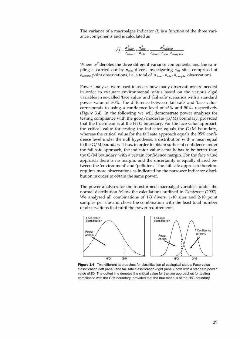
Power analyses were used to assess how many observations are needed in order to evaluate environmental status based on the various algal variables in so-called 'face value' and 'fail safe' scenarios with a standard power value of 80%. The difference between 'fail safe' and 'face value' corresponds to using a confidence level of 95% and 50%, respectively (Figure 3.4). In the following we will demonstrate power analyses for testing compliance with the good/moderate (G/M) boundary, provided that the true mean is at the H/G boundary. For the face value approach the critical value for testing the indicator equals the G/M boundary, whereas the critical value for the fail safe approach equals the 95% confi-dence level under the null hypothesis, a distribution with a mean equal to the G/M boundary. Thus, in order to obtain sufficient confidence under the fail safe approach, the indicator value actually has to be better than the G/M boundary with a certain confidence margin. For the face value approach there is no margin, and the uncertainty is equally shared be-tween the 'environment' and 'polluters'. The fail safe approach therefore requires more observations as indicated by the narrower indicator distri-bution in order to obtain the same power.
The power analyses for the transformed macroalgal variables under the normal distribution follow the calculations outlined in Carstensen (2007). We analysed all combinations of 1-3 divers, 1-10 sites and 2-10 point samples per site and chose the combination with the least total number of observations that fulfil the power requirements.
Figure 3.4 Two different approaches for classification of ecological status: Face-value classification (left panel) and fail safe classification (right panel), both with a standard power value of 80. The dotted line denotes the critical value for the two approaches for testing compliance with the G/M boundary, provided that the true mean is at the H/G boundary.
29
3.4 Results
3.4.1 Descriptive analyses of the algal community
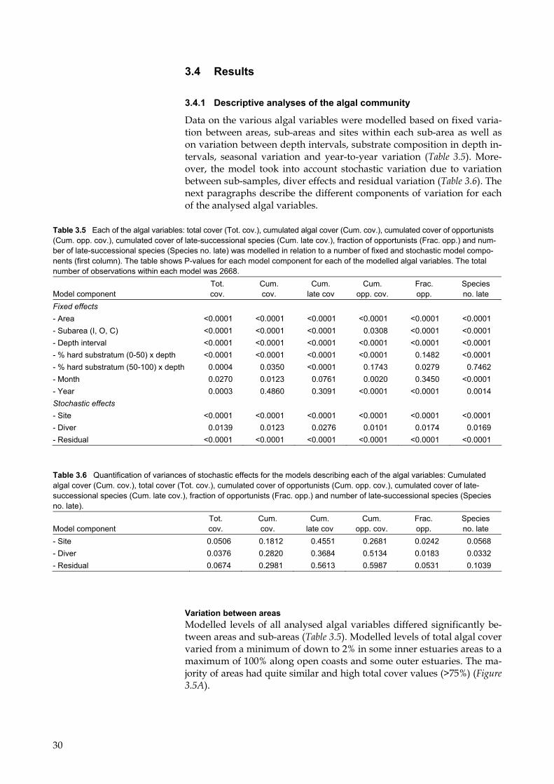
Data on the various algal variables were modelled based on fixed varia-tion between areas, sub-areas and sites within each sub-area as well as on variation between depth intervals, substrate composition in depth in-tervals, seasonal variation and year-to-year variation (Table 3.5). More-over, the model took into account stochastic variation due to variation between sub-samples, diver effects and residual variation (Table 3.6). The next paragraphs describe the different components of variation for each of the analysed algal variables.
Table 3.5 Each of the algal variables: total cover (Tot. cov.), cumulated algal cover (Cum. cov.), cumulated cover of opportunists (Cum. opp. cov.), cumulated cover of late-successional species (Cum. late cov.), fraction of opportunists (Frac. opp.) and num-ber of late-successional species (Species no. late) was modelled in relation to a number of fixed and stochastic model compo-nents (first column). The table shows P-values for each model component for each of the modelled algal variables. The total number of observations within each model was 2668.
Model component Tot. cov.
Cum. cov.
Cum. late cov
Cum. opp. cov.
Frac. opp.
Species no. late
Fixed effects - Area <0.0001 <0.0001 <0.0001 <0.0001 <0.0001 <0.0001 - Subarea (I, O, C) <0.0001 <0.0001 <0.0001 0.0308 <0.0001 <0.0001 - Depth interval <0.0001 <0.0001 <0.0001 <0.0001 <0.0001 <0.0001 - % hard substratum (0-50) x depth <0.0001 <0.0001 <0.0001 <0.0001 0.1482 <0.0001 - % hard substratum (50-100) x depth 0.0004 0.0350 <0.0001 0.1743 0.0279 0.7462 - Month 0.0270 0.0123 0.0761 0.0020 0.3450 <0.0001 - Year 0.0003 0.4860 0.3091 <0.0001 <0.0001 0.0014 Stochastic effects - Site <0.0001 <0.0001 <0.0001 <0.0001 <0.0001 <0.0001 - Diver 0.0139 0.0123 0.0276 0.0101 0.0174 0.0169 - Residual <0.0001 <0.0001 <0.0001 <0.0001 <0.0001 <0.0001
Table 3.6 Quantification of variances of stochastic effects for the models describing each of the algal variables: Cumulated algal cover (Cum. cov.), total cover (Tot. cov.), cumulated cover of opportunists (Cum. opp. cov.), cumulated cover of late-successional species (Cum. late cov.), fraction of opportunists (Frac. opp.) and number of late-successional species (Species no. late).
Model component Tot. cov.
Cum. cov.
Cum. late cov
Cum. opp. cov.
Frac. opp.
Species no. late
- Site 0.0506 0.1812 0.4551 0.2681 0.0242 0.0568 - Diver 0.0376 0.2820 0.3684 0.5134 0.0183 0.0332 - Residual 0.0674 0.2981 0.5613 0.5987 0.0531 0.1039
Variation between areas Modelled levels of all analysed algal variables differed significantly be-tween areas and sub-areas (Table 3.5). Modelled levels of total algal cover varied from a minimum of down to 2% in some inner estuaries areas to a maximum of 100% along open coasts and some outer estuaries. The ma-jority of areas had quite similar and high total cover values (>75%) (Figure 3.5A).
30
The levels of mean cumulated algal cover showed the same trend as that of total cover with lowest levels (down to 11%) in protected estuaries and highest levels (up to 342%) along open coasts and outer parts of some es-tuaries (Figure 3.5B).
Modelled cumulated cover of late-successional species was also lowest (down to 0%) in some protected areas and highest along open coasts (up to 274%, Figure 3.5C).
Modelled levels of cumulated cover of opportunistic algae also showed a minimum in some of the sheltered areas (down to <1%) while highest values typically occurred in the southern and easternmost areas, e.g. Nivå Bay and along the coasts of Bornholm (up to 113%, Figure 3.5D). The modelled fraction of opportunists ranged from <1% to a maximum of 100% in Roskilde inner Fjord (Figure 3.5E).
The number of late-successional species in a sub-sample varied from a minimum of <1 in some inner estuaries and brackish areas to a maxi-mum of 12 along some of the open and more saline coastlines.
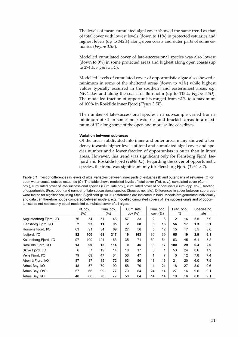
Variation between sub-areas Of the areas subdivided into inner and outer areas many showed a ten-dency towards higher levels of total and cumulated algal cover and spe-cies number and a lower fraction of opportunists in outer than in inner areas. However, this trend was significant only for Flensborg Fjord, Ise-fjord and Roskilde Fjord (Table 3.7). Regarding the cover of opportunistic species, the trend was significant only for Flensborg Fjord (Table 3.7).
Table 3.7 Test of differences in levels of algal variables between inner parts of estuaries (I) and outer parts of estuaries (O) or open water coasts outside estuaries (C). The table shows modelled levels of total cover (Tot. cov.), cumulated cover (Cum. cov.), cumulated cover of late-successional species (Cum. late cov.), cumulated cover of opportunists (Cum. opp. cov.), fraction of opportunists (Frac. opp.) and number of late-successional species (Species no. late). Differences in cover between sub-areas were tested for significance using t-test. Significant (p <0.01) differences are indicated in bold. Models are generated individually and data can therefore not be compared between models; e.g. modelled cumulated covers of late successionals and of oppor-tunists do not necessarily equal modelled cumulated cover of all algae. Tot. cov.
(%) Cum. cov.
(%) Cum. late cov (%)
Cum. opp. cov. (%)
Frac. opp. %
Species no. late
Augustenborg Fjord, I/O 76 54 51 46 57 33 2 6 2 16 5.5 5.9 Flensborg Fjord, I/O 2 93 11 95 2 68 3 16 56 17 1.3 6.1 Horsens Fjord, I/O 63 91 34 69 27 56 5 12 15 17 5.5 8.6 Isefjord, I/O 82 100 68 217 19 163 30 39 65 19 2.9 6.1 Kalundborg Fjord, I/O 97 100 121 163 35 71 59 54 63 45 6.1 8.2 Roskilde Fjord, I/O 13 99 15 114 0 45 13 17 100 29 0.4 2.0 Skive Fjord, I/O 6 7 19 14 10 17 3 1 53 24 0.6 1.9 Vejle Fjord, I/O 79 69 47 64 56 47 1 7 0 12 7.8 7.4 Åbenrå Fjord, I/O 87 87 85 72 63 56 18 16 21 20 6.0 7.9 Århus Bay, I/O 48 57 70 99 58 70 14 24 18 27 8.0 9.6 Århus Bay, O/C 57 66 99 77 70 64 24 14 27 16 9.6 9.1 Århus Bay, I/C 48 66 70 77 58 64 14 14 18 16 8.0 9.1
31

Figur 3.5 Modelled mean level of algal variables in coastal areas/sub-areas. (I) and (O) indicate inner and outer parts of the fjord. A: 'total cover', B: 'cumulated cover', C: cumu-lated cover of late-successional algae. Data are from 2001, 2003 and 2005. Error bars represent confidence intervals. The figure continues on the next page.
32

Figur 3.5 continued Modelled mean level of algal variables in coastal areas/sub-areas. (I) and (O) indicate inner and outer parts of the fjord. D: cumulated cover of opportunistic algae, E: fraction of opportunists, F: number of late-successional species. Data are from 2001, 2003 and 2005. Error bars represent confidence intervals.
33

Figure 3.6 Modelled levels of algal variables as a function of water depth: A: total cover. B: cumulated cover, cumulated cover of late-successional species and cumulated cover of opportunistic algae, C. fraction of opportunists, D: number of late-successional algal species. Data are from 2001, 2003 and 2005.
Variation along depth gradients Modelled levels of all tested algal variables differed significantly be-tween water depths (Table 3.5). As data from the most exposed shallow depth intervals, having low algal cover were excluded in the data analy-ses, the modelled levels of all algal cover variables declined with water depth. Levels of total cover showed a sigmoid decline with depth (Figure 3.6A), whereas cumulated cover declined exponentially with depth (Figure 3.6B). The fraction of opportunists showed a relative minimum in shal-low water and a maximum at 3-7 m depth (Figure 3.6C). The number of late-successional species at 1-3 m depth was about twice as high as in deeper water (Figure 3.6D).
Temporal variation Differences between years were significant for all algal variables except for the cumulated cover and the cumulated cover of late successionals. The average total algal cover was lowest in 2001 and highest in 2003 while 2003 levels were intermediate. Cumulated cover of opportunists increased from 2001 to 2003 and then remained at the same level in 2005
34

while the fraction of opportunists increased over the sampling years. The species number was similar in 2001 and 2003 and slightly lower in 2005.
Seasonal variations were also significant for all variables, except for the cumulated cover of late-successionals and the fraction of opportunists (Table 3.5).
Dependence on substratum composition Modelling of algal variables was improved by taking into account that algal cover varied with the level of hard substratum (Table 3.5). For de-tails see Carstensen et al. (2005).
Stochastic variation in algal cover In addition to the fixed variation due to area, depth, substratum compo-sition in depth intervals and temporal variation, the algal variables are also subject to stochastic variation. The stochastic variation has been subdivided into variation between sites, variation due to diver effects and residual variation (Table 3.6). The residual variation expresses the variation between replicates, i.e. the random variation which is left when the other stochastic effects have been taken into account. In case the model is not perfect, the residual variation also includes variation due to imperfection of the model.
For 'total cover', the residual variance is 0.0674. This equals a standard error of 0.26 (= sqrt 0.0674) of arc. sin. transformed total cover levels or an absolute variance around 16.5% (calculated by up-scaling with Π/2, valid for intermediate coverages). This means that an algal cover value of 50% could typically be represented by observations between 33.5 and 66.5%. If more sites are included in the survey, site-to-site variance, which is slightly smaller than the residual variation, adds to the variabi-lity. Moreover, divers also contribution to random variation, that should be included. Total stochastic variance is 0.1556 which recalculated to to-tal cover values corresponds to about 25% at cover levels of 50%. Thus, a mean total cover of 50% could typically be represented by observations between 25 and 75%. The variance is smaller at the extremes of the scale.
Cumulated cover is even more variable. The residual variation of 0.2981 corresponds to a standard error (se) of 0.55 (= sqrt 0.2981) of the log transformed cumulated cover value. This equals an absolute variation of 73% (calculated as exp(se) = 1 + d, where d is the relative variation). If more sites and different divers are involved, the total variance amounts to 0.7613, corresponding to a variation of about 139%. Thus, a mean cu-mulated cover of 200% might typically be represented by observations in the range 143%-278%.
Stochastic variation of cumulated cover of perennials or opportunistic species is even larger, and those of the fraction of opportunists and the number of late-successional algal species are also large. So, in conclusion, all the algal variables are characterised by large variability.
Gradients within sites We chose 11 areas having a sufficient number of sites to enable the iden-tification of potential spatial gradients. Augustenborg Fjord, Flensborg
35

Fjord, Horsens Fjord, Isefjord, Kalundborg Fjord, Roskilde Fjord, Sejerø Bay, Vejle Fjord, the Sound, Åbenrå Fjord and Århus Bay. In the analysis above with the spatial variation within area described as a step-change between sub-areas, three areas had significant differences between inner and outer parts (Flensborg Fjord, Isefjord and Roskilde Fjord). Changing this to a continuous gradient did not result in more significant spatial variations relative to the results in Table 3.7. Flensborg Fjord showed sig-nificant E-W gradients for all indicators, and Isefjord showed significant gradients for four out of six indicators. Only two indicators (cumulated algal cover and cumulated cover of late-successional species) had signifi-cant N-S gradients for Roskilde Fjord, whereas significant gradients were found in Kalundborg Fjord for cumulated cover of late-successionals and opportunist as well as for the fraction of opportunists. Thus, there were differences in whether the areas had significant step change or continu-ous gradients, but overall there was no general tendency for one gradi-ent model to be better than the other. The step-change in macroalgal ob-servations was very pronounced in Roskilde Fjord, where all sites in the inner part had the same level but sites north of Frederikssund (outer part) had a different level.
This lack of model improvement was also reflected in the estimated vari-ance components for the two different models. For five out of the six macroalgal indicators the site variance actually increased from the step-change to the continuous gradient model (Table 3.8), whereas the diver and residual variance components did not change or increased slightly. This suggests that the continuous gradient model does not provide a significant improvement to describing the spatial variation, and that the spatial variation may only potentially be reduced by inclusion of ex-planatory factors capable of describing the small scale variability in the distribution of macroalgae.
Table 3.8 Quantification of variances of stochastic effects for the models describing each of the algal variables by the two different models (step change vs. linear gradient in grey): Cumulated algal cover (Cum. cov.), total cover (Tot. cov.), cumulated cover of opportunists (Cum. opp. cov.), cumulated cover of late-successional species (Cum. late cov.), fraction of opportunists (Frac. opp.) and number of late-successional species (Species no. late). Results are from 11 selected areas with sufficient sites.
Model component Tot. cov. Cum. cov. Cum.
late cov. Cum.
opp. cov. Frac. opp. Species no. late
- Site w. step change 0.0429 0.1873 0.4866 0.2874 0.0237 0.0798 - Site w. continuous gradient 0.0596 0.2557 0.6820 0.2445 0.0250 0.1098 - Diver w. step change 0.0492 0.3849 0.3915 0.5013 0.0140 0.0386 - Diver w. continuous gradient 0.0544 0.4007 0.4644 0.5337 0.0221 0.0402 - Residual w. step change 0.0726 0.2670 0.4315 0.5494 0.0388 0.0869 - Residual w. continuous gradient 0.0723 0.2651 0.4282 0.5472 0.0387 0.0866
36
3.4.2 Physico-chemical variables
Physico-chemical variables were modelled using the same methodology as for algal variables. Annual mean levels of physico-chemical variables varied markedly between areas (Figure 3.7). Nutrient concentrations were generally highest in inner estuaries and lowest along open coasts. Mod-elled mean concentrations of total phosphorus ranged from 0.53 µM TP at Hesselø to 5.65 µM TP in inner parts of Roskilde Fjord, while concen-trations of inorganic phosphorus ranged from 0.06 µM DIP in Dybsø Fjord to 4.62 µM DIP in inner parts of Roskilde Fjord (Figure 3.7A, B). Modelled mean concentrations of total nitrogen ranged from 18.37 µM TN north of Zealand to 85.33 µM TN in inner parts of Nissum Fjord, while concentrations of inorganic nitrogen ranged from 0.89 µM DIN at Hesselø to 33.81 µM DIN in inner parts of Nissum Fjord (Figure 3.7C, D). Inner estuaries also generally had the most turbid waters with low Sec-chi depths and high concentrations of chlorophyll while open coastal waters had high water clarity and low concentrations of chlorophyll. Area-specific mean Secchi depths ranged from an average of 1.4 m in Nissum Fjord to 13.2 m at the west coast of Bornholm while area-specific mean chlorophyll concentrations ranged from 1.27 µg l-1 in Køge Bay to 7.18 µg l-1 in Skive Fjord (Figure 3.7E, F).
Area-specific mean salinities declined markedly from water bodies in the north-west towards those in the south-east, reflecting the mixing be-tween North Sea water of high salinity and Baltic Sea water of low salinity. Salinity means ranged from an average of 7.3 at the eastern coast of Bornholm to 30.7 in Nissum Broad (Figure 3.7G).
37

Figure 3.7 Mean modelled levels of physico-chemical variables in coastal waters/sub-areas. (I) and (O) indicate inner and outer parts of the fjord. A: concentration of TP, B: concentration of DIP. The figure continues on the next page.
38

Figure 3.7 continued Mean modelled levels of physico-chemical variables in coastal waters/sub-areas. (I) and (O) indicate inner and outer parts of the fjord. C: concentration of TN, D: concentration of DIN. The figure continues on the next page.
39

Figure 3.7 continued Mean modelled levels of physico-chemical variables in coastal waters/sub-areas. (I) and (O) indicate inner and outer parts of the fjord. E: Secchi depth, F: concentration of chlorophyll a, and G: salinity.
40

3.4.3 Algal variables in relation to physico-chemical variables
The area-specific modelled marginal means of algal variables were re-lated to the area-specific modelled means of the physico-chemical vari-ables through multiple regression analysis. In these analyses mean cover levels for each coastal area represented an average water depth of 7 m, a substratum composed of 50% hard bottom and July as the sampling month.
We found a similar tendency for all tested algal variables: they were re-lated to the concentration of total nitrogen and salinity and/or interac-tions between them. An interaction between effects of TN and salinity means that the effect of TN depends on the salinity or vice versa. No other physico-chemical variables improved the relationships (Table 3.9).
All relationships were highly significant and could explain from 66 to 80% of the variation in algal variables (0.6349 <R2 <0.7961, Table 3.9).
Table 3.9 Significant parameter estimates (Est.), coefficients of determination (R2) and levels of significance (p) for relation-ships between algal variables and physico-chemical factors modelled by linear regression analysis. The following algal variables were analysed: Total cover (Tot. cov.), Cumulated algal cover (Cum. cov.), Cumulated cover of late-successional species (Cum. late cov.), Cumulated cover of opportunists (Cum. opp. cov.), fraction of opportunists (Frac. opp.) and number of late-succes-sional species (No. late). Variable TN Salinity Salinity*TN Intercept R2 Est. p Est. p Est. p Est. p Tot. cov. 0.0453 0.0031 -0.0017 <0.0001 1.2304 <0.0001 0.6798 Cum. cov. (log) 0.0914 0.0018 -0.0032 <0.0001 4.5607 <0.0001 0.6953 Cum. late cov. (log) -0.0816 <0.0001 0.1196 0.0001 3.9185 <0.0001 0.7067 Cum. opp. cov. (log) -0.0029 <0.0001 4.6585 <0.0001 0.6941 Frac. opp. 0.0346 <0.0001 -0.0013 <0.0001 0.3595 0.0001 0.6349 No. late 0.1184 <0.0001 -0.0022 <0.0001 0.7923 0.0003 0.7930
As concentrations of total nitrogen (TN) increase, the cover of the total algal community declines (Figure 3.8A) and so does the cumulated cover of the entire community, of the late-successional algae and of the oppor-tunistic algae (Figures 3.8B, C and E) as well as the number of late-succes-sional algal species (Figure 3.8D). In contrast, the fraction of opportunis-tic algal increases with increasing concentrations of TN (Figure 3.8F).
The response of the algal variables to changing nutrient concentrations depended on salinity. Generally the slopes of the regression lines be-tween algal variables and nutrient concentration were steepest at high salinities and the response thus strongest at high salinities. This was the case for total algal cover, cumulated algal cover, cumulated cover of op-portunists and the number of late-successional species (Figures 3.8A, B, D, E). The cover of late-successional species showed parallel regression lines and, thus, the same strength of response at all salinities even though cover levels were higher at higher salinities (Figure 3.8C). Among the in-dicators based on cumulated cover values, the cover of late-successional species showed the steepest regression lines and thus the strongest re-sponse to TN concentrations, while cumulated cover of late-successionals and of opportunists showed a weaker response.
41
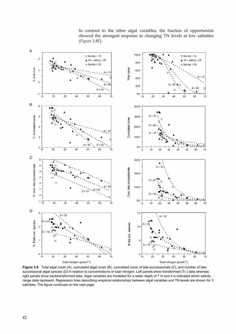
In contrast to the other algal variables, the fraction of opportunists showed the strongest response to changing TN levels at low salinities (Figure 3.8F).
Figure 3.8 Total algal cover (A), cumulated algal cover (B), cumulated cover of late-successionals (C), and number of late-successional algal species (D) in relation to concentrations of total nitrogen. Left panels show transformed (Tr.) data whereas right panels show backtransformed data. Algal variables are modelled for a water depth of 7 m and it is indicated which salinity range data represent. Regression lines describing empirical relationships between algal variables and TN-levels are shown for 3 salinities. The figure continues on the next page.
42

Figure 3.8 continued Cumulated cover of opportunists (E), and fraction of opportunists (F) in relation to concentrations of total nitrogen. Left panels show transformed (Tr.) data whereas right panels show backtransformed data. Algal variables are mod-elled for a water depth of 7 m and it is indicated which salinity range data represent. Regression lines describing empirical rela-tionships between algal variables and TN-levels are shown for 3 salinities.
3.4.4 The "Spanish Index" tested on Danish macroalgal data
A prerequisite for the "Spanish index" is that it reflects negative antropo-genic influence on the marine environment. As it appears in the previous section, the cover of late-successional species, the fraction of opportunists as well as the number of late-successional species were all related to con-centrations of total nitrogen (Table 3.9, Figures. 3.8B, E and F). The crite-rion for including these variables in the index was thus fulfilled for Dan-ish coastal areas.
The "Spanish index" operates with just two depth intervals. We found, not surprisingly, that each of the three components were depth dependent (Table 3.5) and showed marked changes with depth (Figure 3.6). Hard substrate in Danish waters is made up of boulders and stones nearly eve-rywhere with changing depth distribution from site to site. Moreover, hard bottom is generally found on deeper waters in open and less pol-luted waters compared to sheltered fjords. This depth dependence and distribution pattern of hard substrate are not compatible with a scoring system with just two depth ranges. Rather, the depth dependence of the algal components must be better integrated in the scoring system.
We also found that the level of algal components in the index varied markedly between areas (Table 3.5) and that salinity was an important variable affecting the algae (Table 3.9, Figure 3.7). The salinity will then have a strong influence in the index scores.
43

3.4.5 Reference levels and class borders sensu WFD for macroalgal variables
For each of the estuaries/coastal areas we entered the TN-levels defining reference levels and class boundaries (Table 2.4 in chapter 2) and annual mean salinities (shown in Figure 3.7G) in the empirical relationships (de-fined in Table 3.9). We thereby calculated the level of algal variables de-fining reference conditions and class boundaries (Appendices 1-6). The level of the boundaries, the variability associated with them and the width of the status classes differ widely between variables and between areas. The applicability of the algal variables for assessment of water quality thus also varies between variables and areas.
In order for an algal variable to be applicable for assessment of ecological status, the class borders should be defined with low variability and the status class bands should be relatively broad. This demand was best ful-filled for the variables which were associated with a low degree of sto-chastic variability and a strong response to changes in TN concentrations.
The variables 'total cover', and 'number of late-successional species' gen-erally showed relatively low stochastic variability and a strong response to TN concentration at high salinities so these indicators had class bor-ders with relatively low variability in high salinity areas (Table 3.6). The 'fraction of opportunists' also had relatively limited stochastic variability with weak responses to changing TN concentrations at high salinities. So class borders of this variable generally showed high variability and nar-row status class bands in high salinity areas. By contrast, in low salinity areas where responses to TN were stronger, class borders were defined with less variability.
The cumulated algal cover variables were associated with more stochastic variability than the algal variables mentioned above and therefore tended to have class borders connected with relatively large variability.
The response of TN concentration to changes in TN loading in a given area also affects the width of the status class. Thus, areas which demon-strate a strong response in TN upon changes in N-loading, i.e. areas hav-ing a large regression slope for the regression of TN-concentration upon TN-input (chapter 2, Figure 2.6) have broader status class bands than areas showing a weak response to TN inputs. Many open areas, such as Born-holm, show weak responses in TN to changing TN inputs and, therefore, have narrow status class bands. By contrast, areas with significant nutri-ent sources and low water exchange such as inner Odense Fjord, several Limfjord basins, Randers and Nissum Fjords show strong responses in TN concentration to changes in TN inputs and therefore have broader status class bands. The demand for the indicators to have low stochastic variability and high sensitivity to TN is intensified if the area in question has narrow status class bands for TN.
For the Sound, Nivå Bay, Limfjorden west of Mors and Roskilde Fjord we have illustrated the class boundaries and their associated variability together with actual levels of the algal indicators (Figures 3.9 - 3.12). These figures illustrate that status class bands are narrow in the Sound and Nivå Bay – areas with a weak response of TN concentrations to TN
44

inputs (Figures 3.9 and 3.10) whereas they are much broader in Limfjor-den west of Mors and Roskilde Fjord – areas with a strong response of TN concentration to TN inputs (Figures 3.11 and 3.12). All cover indica-tors have been estimated to a standard depth of 7 m for comparison across areas. This depth standardisation will reduce the indicator preci-sion for those sites with few data around 7 m, and in such cases it will be more appropriate to choose a standardisation depth representing an av-erage depth for the area.
The figures also illustrate that along the open coasts of the Sound and Nivå Bay, status class bands of total cover were close to 100% and all very narrow. This is because total cover levels are potentially high in the open areas and often reach the upper boundary of 100%. Therefore, fu-ture modelling of total cover levels and class boundaries for open coastal areas should represent a water depth of 9 m where light limitation is more intense and where cover levels consequently are lower than at a depth of 7 m.
In Limfjorden west of Mors status class boundaries were well separated for all variables except for the fraction of opportunists (Figure 3.11). The narrow status class bands for the fraction of opportunists in this area are due to the high salinities which weaken the response of the fraction of opportunists to TN (Figure 3.8).
For the Sound and Nivå Bay, the mean levels of the algal indicators for the years 2001-2005 typically fell within the status class 'bad'. The rela-tively low TN levels of the Sound thus give expectations of higher levels of algal cover and numbers of perennial species and lower fractions of opportunists than found. Based on the Swedish macrophyte index, the ecological status of the northern Sound is assessed as moderate (http://www.viss.lst.se/; district= Södra Östersjön, vattenkategori=Kust; Öresund).
45

A
Tota
l alg
al c
over
(%)
Ref. H-G G-M M-P P-B 2001 2003 2005
40
60
80
100
B
Cum
ulat
ed a
lgal
cov
er (%
)
Ref. H-G G-M M-P P-B 2001 2003 20050
50
100
150
200
250
HIGHGOOD
MODERATE
BAD
POOR
BAD
C
Cum
. cov
er o
f lat
e su
cces
sion
als
(%)
Ref. H-G G-M M-P P-B 2001 2003 20050
20
40
60
80
100
120
140
HIGHGOOD
MODERATE
D
Cum
. cov
er o
f opp
ortu
nist
s (%
)
Ref. H-G G-M M-P P-B 2001 2003 20050
20
40
60
80
100200225
HIGH GOODMODERATE
POOR
BADBAD
POOR
E
Frac
tion
of o
ppor
tuni
sts
(%)
Ref. H-G G-M M-P P-B 2001 2003 200520
30
40
50
60
70
80
F
Num
ber o
f lat
e su
cces
sion
als
Ref. H-G G-M M-P P-B 2001 2003 20052
3
4
5
6
7
8
9
HIGHGOOD
MODERATEPOORBAD
BADPOOR
MODERATEHIGHGOOD
Figure 3.9 Reference levels, class borders and actual levels of various algal variables in the Sound: Total algal cover (A), Cumulated algal cover (B), Cumulated cover of late-successionals (C), Cumulated cover of opportunists (D), fraction of oppor-tunists (E) and number of late-successional algal species (F). Algal variables are modelled for a water depth of 7 m.
46

A
Tota
l alg
al c
over
(%)
Ref. H-G G-M M-P P-B 2001 2003 20050
255075
80
85
90
95
100B
Cum
ulat
ed a
lgal
cov
er (%
)
Ref. H-G G-M M-P P-B 2001 2003 20050
255075
100125150175200225250375450
HIGH GOODMODERATE
HIGH GOODMODERATE
POORBAD
POORBAD
C
Cum
. cov
er o
f lat
e su
cces
sion
als
(%)
Ref. H-G G-M M-P P-B 2001 2003 20050
20
40
60
80
100
120
HIGHGOOD
MODERATE
D
Cum
. cov
er o
f poo
rtuni
sts
(%)
Ref. H-G G-M M-P P-B 2001 2003 200520
40
60
80
100
120
140
160400500
HIGH GOODMODERATE
POOR
BAD
BADPOOR
F
Num
ber o
f lat
e su
cces
sion
als
Ref. H-G G-M M-P P-B 2001 2003 20051
2
3
4
5
6
7
8
9
HIGHGOOD
MODERATE
E
Frac
tion
of o
ppor
tuni
sts
(%)
Ref. H-G G-M M-P P-B 2001 2003 200520
40
60
80
100
POORBAD
BADPOORMODERATEGOODHIGH
Figure 3.10 Reference levels, class borders and actual levels of various algal variables in Nivå Bay: Total algal cover (A), Cumulated algal cover (B), Cumulated cover of late-successionals (C), Cumulated cover of opportunists (D), fraction of oppor-tunists (E) and number of late-successional algal species (F). Algal variables are modelled for a water depth of 7 m.
47

A
Tota
l alg
al c
over
(%)
Ref. H-G G-M M-P P-B 2001 2003 20050
20
40
60
80
100HIGH
GOOD
MODERATE
B
Cum
ulat
ed a
lgal
cov
er (%
)
Ref. H-G G-M M-P P-B 2001 2003 20050
50
100
150
200
250
300
HIGH
GOOD
MODERATE
C
Cum
. cov
er o
f lat
e su
cces
sion
als
(%)
Ref. H-G G-M M-P P-B 2001 2003 20050
50
100
150
200
250
HIGH
GOOD
MODERATEPOOR
D
Cum
. cov
er o
f opp
ortu
nist
s (%
) Ref. H-G G-M M-P P-B 2001 2003 2005
0
5
10
15
20
25
HIGH
GOOD
MODERATE
E
Frac
tion
of o
ppor
tuni
sts
(%)
Ref. H-G G-M M-P P-B 2001 2003 2005
0
5
10
15
205075
100
HIGHGOODMODERATEPOORBAD
F
No.
of s
ucce
ssio
nals
Ref. H-G G-M M-P P-B 2001 2003 2005
0
5
10
15
20
HIGH
GOOD
MODERATEPOOR
Figure 3.11 Reference levels, class borders and actual levels of various algal variables in Limfjorden west of Mors: Total algal cover (A), Cumulated algal cover (B), Cumulated cover of late-successionals (C), Cumulated cover of opportunists (D), fraction of opportunists (E) and number of late-successional algal species (F). Algal variables are modelled for a water depth of 7 m.
48

A
Tota
l alg
al c
over
(%)
Ref. H-G G-M M-P P-B 2001 2003 20050
20
40
60
80
100
HIGH
GOOD
MODERATE
B
Cum
ulat
ed a
lgal
cov
er (%
)
Ref. H-G G-M M-P P-B 2001 2003 20050
20
40
60
80
100
120
140
HIGH
GOOD
MODERATEPOORBAD
C
Cum
. cov
er o
f lat
e su
cces
sion
als
(%)
Ref. H-G G-M M-P P-B 2001 2003 2005
0
5
10
15
20
25
30
35
HIGH
GOOD
MODERATE
D
Cum
. cov
er o
f opp
ortu
nist
s (%
)
Ref. H-G G-M M-P P-B 2001 2003 20050
10
20
30
40
50
60
HIGH
GOOD
MODERATE
POORBAD
F
Num
ber o
f lat
e su
cces
sion
als
Ref. H-G G-M M-P P-B 2001 2003 2005-1
0
1
2
3
4
5
HIGH
GOOD
MODERATE
E
Frac
tion
of o
ppor
tuni
sts
(%)
Ref. H-G G-M M-P P-B 2001 2003 200550
60
70
80
90
100
GOOD
HIGH
POORBAD
Figure 3.12 Reference levels, class borders and actual levels of various algal variables in Roskilde Fjord: Total algal cover (A), Cumulated algal cover (B), Cumulated cover of late-successionals (C), Cumulated cover of opportunists (D), fraction of oppor-tunists (E) and number of late-successional algal species (F). Algal variables are modelled for a water depth of 7 m.
The mean levels of the algal indicators in Limfjorden west of Mors were typically within the status class moderate. Modelled mean levels of each algal variable in each area are shown in Appendices 7-12.
3.4.6 Sensitivity of the algal variables
The variance of the residual variation was the largest of the three com-ponents of stochastic variation, but the variance contribution from divers and sites was also considerable (Table 3.6). Therefore, as a general rule of thumb, all these components should be reduced by increasing both the number of divers, sites and point samples per site in order to obtain more precise results.
49

The least number of observations necessary to evaluate environmental status based on the various algal variables in face value and fail safe clas-sification scenarios with a standard power value of 80% are shown in Appendices 13-18. Results are shown for all areas which fulfilled the power requirements within combinations of 1-3 divers, 1-10 sites and 2-10 point samples per site.
The fail safe approach always required more observations than the face value approach and in many cases the fail value approach could not ful-fil the power requirements within the combinations of 1-3 divers, 1-10 sites and 2-10 point samples per site.
The least number of observations necessary to fulfil the power require-ments also varied considerably among variables. The power demands were best fulfilled for the variables 'total cover', 'fraction of opportunists' and 'number of late-successional species'. Of the 44 areas/sub-areas exa-mined 19 fulfilled the power demands in the face value scenario and 11 fulfilled the demands for the fail safe scenario with regard to the variable 'total cover' (Appendix 13). The corresponding numbers for the number of late-successionals were 19 and 10 (Appendix 18), and for the fraction of opportunists 16 and 2 areas fulfilled the requirements (Appendix 17).
Only few areas fulfilled the power demands with respect to the cumu-lated cover variables. Eight areas fulfilled the power demands in the face value scenario while no areas fulfilled the demands for the fail safe sce-nario with regard to the variable 'cumulated algal cover' (Appendix 14). The corresponding numbers for the 'cumulated cover of late-succes-sionals' were 6 and 2 (Appendix 15), and for 'cumulated cover of oppor-tunists' 9 and 1 areas fulfilled the requirements (Appendix 16).
The numbers of sub-samples needed to fulfil the requirements at one sampling depth in a given area/sub-area varied from 2 to 90, but in most cases below 20 samples were needed. For illustration, an annual sampling intensity of e.g. 5 sites with 3 sub-samples per depth interval and only one diver results in 15 observations per area/sub-area per year and 45 observations if data from 3 years are pooled.
3.5 Discussion
3.5.1 Algal variables in relation to nutrient and salinity gradients
All tested algal variables responded to changes in concentrations of total nitrogen and salinity. The regulating mechanisms thus seem to be very uniform among variables.
Such uniformity has not been apparent in our earlier analyses which were based on fewer data sets (Carstensen et al. 2005). The uniformity has emerged after we have included additional data and refined the algal models. Very large data sets were apparently necessary in order to iden-tify patterns hidden in a jungle of variability.
50

A response to changes in nutrient concentration is a prerequisite for us-ing the algal variables as indicators of eutrophication. This prerequisite was thus found to be fulfilled for all the variables even though the strength of coupling to TN concentration varied between variables and typically also depended on salinity.
Cumulated cover of opportunistic species showed a negative response to TN – in opposition to most previous findings. The reason for this is probably that our study focused on algae growing in deeper waters where opportunists as well as late-successionals are light limited. The positive effect of improved water quality on cover of opportunistic macroalgae in deeper water can thus be explained by the better light conditions for growth as nutrient concentrations decrease.
In open areas such as along the open coasts of the Sound and Nivå Bay, status class bands of total cover were close to 100% and all very narrow. This is in part because these areas have a weak response of TN concen-trations to TN inputs and in part because total cover levels are poten-tially high in the open areas and often reach the upper boundary of 100%. Only few samples represent water depths >10 m where light at-tenuation more markedly affects the open water algal communities. Deeper located algal communities in open waters such as the stone reef algae do show clear responses to changes in nutrient load (Dahl & Car-stensen 2008).
The fraction of opportunists increased with increasing concentrations of TN, as expected. This response did not appear in our earlier analyses where the fraction of opportunists was found to respond solely to changes in salinity (Carstensen et al. 2005). The larger data sets used in this analysis have made it possible to detect a response to TN. This re-sponse was strongest at low salinities where more opportunistic species are present and weaker at higher salinities where cover levels of oppor-tunists are low.
The positive effect of salinity on the number of algal species is in accor-dance with earlier reports of increases in the total number of macroalgal species along the Baltic salinity gradient (Nielsen et al. 1995) and in Dan-ish estuaries (Middelboe et al. 1998). It can be explained by the fact that more species are adapted to marine than to brackish conditions. The lar-ger diversity at higher salinities may also explain the higher cover levels of the algal community at higher salinities because the many species rep-resenting various life forms and forming a multi-layered community should be able to exploit the incoming light more efficiently and thus be more productive and dense than a less diverse community (Spehn et al. 2000). The methodology used in our study also generates a higher likeli-hood of obtaining high levels of cumulated cover when more species are present, because even if one species grows in more layers, its maximum possible cover is 100%.
Our results also showed that salinity affects the ratio between late-successional and opportunistic species. Again this is in accordance with large scale studies from the Baltic Sea, showing that the classes of red and brown algae, which contain most of the late-successional species,
51

prevail at high salinities, while green algae which contain many oppor-tunists prevail at low salinities (Nielsen et al. 1995). Other variables than salinity do, however, also affect the gradients of macroalgal distribution across the Baltic Sea (e.g. Middelboe et al. 1997).
3.5.2 Variability of algal variables
Another important characteristic of a good indicator is that it can be as-sessed precisely, i.e. with low stochastic variability.
All algal variables were found to be associated with considerable vari-ability (Table 3.6). The variables showing least stochastic variability were total cover, fraction of opportunists (in areas with low salinity) and num-ber of late-successional species.
The variables expressing cumulated cover showed much more variability – especially the cumulated cover of late-successionals and the cumulated cover of opportunists. The higher variability of cumulated cover levels relative to total cover levels is most likely due to the fact that the cumu-lated levels are sums of cover observations with associated variability and thus also accumulate this variability. The reason why cumulated cover of opportunists and of late-successional species are more variable than cumulated cover of the entire algal community may be that there is more natural variability connected with the specific algae which colonise the substrates in a given area than with the total colonisation of the sub-strates. This would imply that sub-samples differ more with respect to the cumulated cover of perennials and opportunists than with respect to cumulated cover of all species.
The power analyses confirmed the patterns indicated by the stochastic variability but also demonstrated that the number of observations needed in order to assess ecological status with sufficient accuracy strongly de-pends on the type of the estuary/coastal area in question. Thus, areas with weak responses of TN concentration to TN input demanded more observations than areas with strong TN responses.
A further reduction of the stochastic variation of the algal variables re-quires that diver variation is reduced and that effects of site-specific fea-tures such as currents and bottom topography are adequately described. Biologic interaction like space competition between macroalgal vegeta-tion and blue mussels (Mytilus edulis) or sea squirts (Ciona intestinalis) are also likely to contribute to the observed stochastic variation.
3.5.3 Choice of algal indicators
The best algal indicators are those which reflect nutrient gradients as clearly as possible and which are associated with low variability. Based on these criteria and the discussions of the previous two sections total algal cover and number of perennial algal species together with the frac-tion of opportunists in areas of low salinity were the most promising among the potential algal indicators. However, it is important to keep in mind that the indicator total algal cover needs deeper sampling stations to provide useful data compared to indicators using cumulative cover.
52

In its present form the Spanish index was found not to be applicable to Danish conditions. One reason is that we found each of the three compo-nents of the index to change markedly with depth (Table 3.5, Figure 3.6). This depth dependence is not compatible with a scoring system with just two depth ranges (5-15 m and 15-25 m) as defined for the Spanish index. Rather, the depth dependence of the algal components must be better in-tegrated in the scoring system in order to be useful for Danish waters. If this adjustment is not incorporated in the index, we risk misinterpreting the ecological status. For example, with the present version of the Span-ish index, a site having a high algal cover – but only to a depth of 6 m –may obtain a better score than sites with algal communities of limited cover at a depth of 15 m.
We also found that the level of each of the three algal components of the Spanish index varied markedly between areas (Table 3.5) and that salinity was an important variable affecting each component of the index (Table 3.9, Figure 3.8). In order to be useful for Danish conditions, the scoring system must therefore also take salinity into account.
Moreover, the scoring system must be adjusted to Danish conditions. First of all it must be adjusted to the range of the Danish algal variables which differ from that of the Spanish variables. In addition, we find it necessary to base the definition of reference values and class borders on documented changes in the level of algal components with changing TN levels as identified in our empirical models.
3.5.4 Use of algal variables to assess ecological status according to the Water Framework Directive
The present study identified the algal variables 'total algal cover' and 'number of late-successional algal species' together with the 'fraction of opportunists' in areas of low salinity as the most promising among the potential algal indicators. Assessment of water quality based on these variables seems most feasible for areas showing strong responses of TN concentration to TN input and thereby having relatively well separated ecological status classes. Still, however, the algal indicators are connected with considerable variability which renders precise assessment of eco-logical status difficult. With these limitations in mind, we here provide a stepwise guidance with a diagram on how to assess ecological status in the future, based on the most promising algal variables (Figure 3.13):
Choice 1: Use the present model which is based on algal- and physico-chemical data from 2001, 2003 and 2005 as a basis for the assessment.
• Collection of algal data Collect new algal data along the depth gradients of the area to be as-
sessed.
• Normalisation of data Normalise the new algal data taking into account sampling sites,
sampling depths, substratum cover and sampling month in order to estimate a mean value representing a water depth of 7 m, 50% cover of hard substratum and July as the sampling month. This procedure
53

renders the new data set comparable to the data defining the ecologi-cal quality classes and also defines associated confidence levels. The normalization procedure needs advanced statistical tools like 'SAS'. A web based access to a normalization procedure at the National Marine Monitoring Data Centre at NERI could be a way forward for users in the future.
• Assessment of ecological quality Compare the normalised algal data with the ecological quality classes
and thereby assess ecological status.
Choice 2: Improve the model based on new algal and physico-chemical data col-lected in the future and use the improved model as a basis for the assessment.
• Collection of algal and physicochemical data Include new data sets of algal and physico-chemical variables for 2007,
2009, … to supplement the existing data from 2001, 2003 and 2005. • Update the model with the new data Use the new data series to update the existing model, thereby estab-
lishing new borders of the ecological quality classes. • Assess ecological status
Compare the newest data set (e.g. 2009) of a given area with the bor-ders defining the quality classes and thereby assess the ecological status.
Further development of the model is recommended as new data sets be-come available in the coming years and a larger data set is expected to improve the accuracy of the ecological quality classes of the different al-gal indicators. Nitrogen load figures used to define the borders of eco-logical classes might also change in the coming years as knowledge im-proves.
Figure 3.13 Stepwise guidance on future practical use of the algal model to assess ecological status, based on the most prom-ising algal variables.
54

3.6 Conclusions
• All algal variables responded to changes in TN and thereby fulfil an important prerequisite for use as indicators of water quality.
• All algal variables also responded to changes in salinity and thereby
highlight the need for setting different targets depending on salinity. • The algal variables showed a large generality in responses as TN and
salinity are the main factors regulating them all. The variables were, however, associated with considerable variability due to diver effects, variation between sites and residual variation.
• Each of the components of the Spanish index responded to nutrient
gradients in Danish coastal waters, but the index would need marked adjustments, especially in the scoring system, in order to be applicable to Danish conditions.
• Our analyses indicate that the most promising indicators, i.e. those
that show the strongest response to nutrient gradients and are associ-ated with least variability are the following: 'total algal cover', 'num-ber of late-successional species' and 'fraction of opportunists'.
• Assessment of water quality based on these variables seems most fea-
sible for areas showing strong responses of TN concentration to TN input and thereby having relatively well separated ecological status classes.
• With the above limitations in mind, the study describes how to assess
ecological status in the future, based on the most promising algal variables.
55

4 Assessment of ecological status using chlorophyll a
4.1 Boundaries for chlorophyll a
Summer primary production in Danish coastal waters is nitrogen limited due to the exchange with phosphate-rich open waters. Therefore, the summer phytoplankton biomass is considered related to the nitrogen levels. Dissolved inorganic nitrogen (DIN) in winter has previously been considered a good indicator for the phytoplankton biomass potential, especially in deeper open waters where mixing depths exceed the photic depths until around March when the spring bloom occurs. This mecha-nism does, however, not apply to shallow coastal waters where primary production and phytoplankton biomass can be considerable even in win-ter. Secondly, DIN is a highly fluctuating variable and the relatively few observations over a winter period does not give sufficient precision for estimating the mean level. Consequently, total nitrogen is a more robust variable that is directly related to nitrogen inputs from land and a large fraction of TN is bioavailable, particularly if a large part of TN has terres-trial origin. TN is considered composed of a bioavailable and a refractory part, and it is believed that there is a generic functional relationship be-tween phytoplankton biomass and bioavailable nitrogen, whereas the frac-tion of bioavailable nitrogen depends on site-specific features such as in-fluence of terrestrial nitrogen, retention time and exchange with Baltic Sea water that has a relatively high refractory part of TN.
Let us assume that we can describe the generic relationship between phytoplankton biomass, proxied by chlorophyll a (chla), and bioavailable TN by means of a power function:
bbb TNlebioavailabpalebioavailabTNachla ⋅⋅=⋅= )()(
where p(bioavailable) is the bioavailable proportion of TN. Using a log-trans-form on this equation yields
)log())(log()log()log( TNblebioavailabpbachla ⋅+⋅+=
which is a linear relationship between log(TN) and log(chla) with an inter-cept, log(a), that is site-dependent. The site-specific relationships were es-timated to analyse commonalities in the slopes (Figure 4.1). A total of 19 sites had significant slopes with 2 of these actually showing negative re-lationships between chla and TN (Mariager Fjord and Ringkøbing Fjord after change of sluice practice). Mariager Fjord is the only true fjord in Denmark with a sill, permanent stratification and hypoxia/anoxia below the pycnocline. Mussels in high densities are present along the shores above the pycnocline, but grazing pressure in the deeper part, where the monitoring station is located, is limited because the poor oxygen condi-tions in the deep water gives little zooplankton recruitment. Consequent-ly, other mechanisms than bottom-up control may be more important for the summer phytoplankton biomass. Ringkøbing Fjord experienced a re-
56

gime shift after changing the sluice practice in 1995 raising the salinity level (Petersen et al. 2008). One of several consequences was that mussel colonisation changed the sediment characteristics substantially, increas-ing oxygen penetration through bioturbation. This increased the sedi-ment capacity to iron-bind phosphate and for phytoplankton the conse-quence was that primary production became phosphorus limited. Only in recent years Ringkøbing Fjord appears to be switching back to nitro-gen limitation. Therefore, TN cannot be expected to control phytoplank-ton biomass for the period after 1995. These two sites will thus not be used for establishing a generic relationship between chla and TN.
All other sites, except for Køge Bay, had confidence intervals for esti-mated slopes that could contain values in the range between 0 and 1, which is the expected slope range reflecting a decreasing yield of chla for increasing TN. Slopes above 1 would reflect progressively increasing chla with TN, which is contradictory to the general ecological theory. Most of the slope estimates were in the range from 0.2 to 0.85, however, with a group of 6 sites having estimated slopes above 1.
Figure 4.1 Ranked estimated slopes for a linear relationship between log-transformed TN and chla. Non-significant slopes (p >0.05) have open symbols and significant slopes (p <0.05) have filled symbols. Error bars show the 95% confidence interval of the estimated slopes.
Given that most slopes had comparable values, despite some of them were based on relatively few years, and that the theory outlined above prescribes that the slope should be generic, whereas the intercept should be site-specific, the relationship for log(chla) was formulated into a statisti-cal model as
)log()log( TNbsitechla ⋅+=
which for the non-transformed variables corresponds to a power func-tional relationship as
chla = k(site) × TNb
57

The statistical analysis was carried out on log-transformed variables (Figure 4.2), and the common factor (b) was estimated as 0.55 (±0.05). The site-specific factors varied from 0.16 to 2.96, typically lower for coastal sites with the exception of Dybsø Fjord and increasing as the estuaries/ coastal sites become more enclosed (Figure 4.3). Two sites, Nissum Fjord and Ringkøbing Fjord before change of sluice practice, had very high fac-tors giving unrealistically high chla yields compared to TN when using Redfield ratios and a carbon:chla ratio of 50 for conversion. This indi-cates that additional nitrogen is introduced to these systems. In fact, both systems have been dominated by cyanobacteria (ca. 33% and 80% for Nissum Fjord and Ringkøbing Fjord, respectively) and this additional ni-trogen input may have come from nitrogen fixation. Thus, the conse-quence of this is that chla-TN relationships as described here are not ap-plicable to coastal systems with a large proportion of nitrogen-fixing cyanobacteria, particularly if the proportion of cyanobacteria varies greatly from year to year.
Figure 4.2 Summer chla versus winter-spring TN mean concentrations for 42 different sites. Solid line shows the estimated relationship averaged over all sites, and dotted lines show relationship with the lowest factor (Dybsø Fjord) and the highest factor (Ringkøbing Fjord before change of sluice practice).
58

Figure 4.3 Estimated site-specific factors ranked by magnitude. Error bars show the 95% confidence intervals of the estimates.
The site-specific factors estimated from the chla-TN relationships de-scribed the fraction of TN available for phytoplankton biomass and to verify this assumption the bioavailable fraction was calculated during the winter months (January-February) when most of the bioavailable frac-tion was either in the form of dissolved inorganic nitrogen (DIN) or phy-toplankton biomass. Therefore, the bioavailable nitrogen was calculated as the sum of DIN and chla converted to nitrogen by means of Redfield ratios and a carbon : chla ratio of 50.
Indeed, most sites showed a good agreement between the estimated fac-tors and the winter bio-available nitrogen fraction (Figure 4.4). The inter-cept of the regression was not significantly different from zero (p = 0.9132) resulting in a proportional relationship between the bioavailable nitrogen fraction in winter and the estimated site-specific yield factor from the chla-TN regression. This is in agreement with the conceptual theory. There were, however, a number of sites that deviated from the overall pattern. Randers Fjord and Odense Fjord inner part are strongly influenced, particularly in winter time, by riverine inputs. These two sites deviate because 1) TN in January-June may not be a good nutrient status indicator for summer chla due to low retention times and 2) phy-toplankton primary production in summer may additionally be limited by high flushing rates and light limitation. Skive Fjord is very productive with high biomasses throughout summer and summer algae blooms are fuelled by nutrients from the sediments following events of hypoxia (Carstensen et al. 2007). In this sense Skive Fjord behaves partly like Mariager Fjord with an intensified internal recycling of nutrients and no benthic grazing in the deeper parts where the monitoring station is lo-cated. Finally, Dybsø Fjord has a lower chla yield from TN than most other sites. The exact reason for this is not known.
59

Figure 4.4 Estimated site-specific factor from chla-TN rela-tionship versus estimated bio-available nitrogen fraction in January and February. Nissum Fjord and Ringkøbing Fjord be-fore change of sluice practice are not shown due to high factors (2.0 and 3.0, respectively). Open symbols with identified sites show sites that also deviated from the overall trend.
For the analysis above it has been assumed that the relationship between chla and TN could be described by a power function, which is a reason-able flexible function for curve fitting. However, to investigate the ap-propriateness of this function, an alternative relationship was investi-gated assuming a quadratic response for the log-transformed variables (Smith 2006). The rationale behind this response was the observation of a strong curvilinear relationship when pooling data from 92 marine sites, although site-specific features were neglected.
Figure 4.5 Estimated chla-TN relationship using linear and quadratic response compared to the relationship reported by Smith (2006). Data from Mariager Fjord, Nissum Fjord and Ringkøbing Fjord were not used. Dotted lines show relationship with the lowest factor (Dybsø Fjord) and the highest factor (Skive Fjord).
Investigating the present data set using a quadratic response with a site-specific intercept in comparison to the linear response described above gave a marginally significant and a slight improvement in the coefficient of determination (from R2 = 87.9% to 88.1%), but the strong curvilinear response suggested by Smith (2006) was not observed (Figure 4.5). More-over, the annual means in the cross-system analysis of Smith (2006) can-not be directly compared to the seasonal means used for the present study. The significance of the quadratic response was driven by data
60

from Randers Fjord and Odense Fjord inner part only, and as described above it is questionable whether these sites actually fulfil the require-ments for establishing a generic chla-TN relationship. Consequently, the linear relationship was chosen.
Reference conditions and boundary values were calculated from the chla-TN regression using the corresponding values for TN as input (Table 4.1). Standard errors for these estimates were found by Monte Carlo simulation taking variations in the estimated model as well as uncer-tainty of the TN reference condition and boundary values into account. There were only minor differences in the reference conditions and boundary values of Table 4.1 to those reported for the WFD intercalibra-tion (Carstensen 2006, unpublished).
The boundary between good and moderate was on average 36% above the reference conditions but it varied from 8% in the Sound North to 91% for the outer part of the Wadden Sea. These differences were a combina-tion of the response in TN to nitrogen inputs and the factor used in the chla-TN relationship. It is noteworthy that open water sites along the west coast (Wadden Sea outer part and Hirtshals) and coastal sites ex-changing with the North Sea (Wadden Sea inner part and sites in Lim-fjorden) all had high ratios between G/M boundary and reference condi-tion (>47%) for those reasons.
Reference conditions and boundary values could not be determined for a number of coastal sites that behave differently from the general re-sponses of Danish coastal sites. Ringkøbing Fjord might be included in the analysis after a few more years of monitoring since the cyanobacteria have disappeared and the fjord is becoming nitrogen limited. Nissum Fjord still has a considerable cyanobacteria population and further studies should conclude how to account for their presence. Mariager Fjord has an internal recycling of nutrients that dominates relative to freshwater sources, and models that take such phenomenon into account should be developed specifically for Mariager Fjord. It could also be argued that Randers Fjord, Odense Fjord inner part, Skive Fjord and Dybsø Fjord do not entirely fulfil the assumptions for the approach (ref. Figure 4.4), but until better models are available for these sites the calculated values (Ta-ble 4.1) provide the best estimates.
61

Table 4.1 Suggested reference conditions and boundary values for summer (May-September) chla concentration (µg l-1) com-puted from corresponding values of TN concentrations (Table 2.3) by means of the generic regression model with site-specific factors. Boundary values between good and moderate status are highlighted. Locality Ref. cond. H-G G-M M-P P-B Archipelago of southern Fyn 1.31 (±0.08) 1.40 (±0.10) 1.57 (±0.12) 1.76 (±0.15) 1.87 (±0.17) Augustenborg Fjord 2.79 (±0.51) 3.16 (±0.60) 3.81 (±0.78) 4.50 (±0.98) 4.90 (±1.11) Bornholm W 1.22 (±0.10) 1.25 (±0.12) 1.33 (±0.15) 1.40 (±0.21) 1.45 (±0.23) Dybsø Fjord 0.93 (±0.29) 1.10 (±0.35) 1.37 (±0.46) 1.66 (±0.57) 1.82 (±0.65) Fakse Bay 1.52 (±0.21) 1.57 (±0.24) 1.66 (±0.31) 1.78 (±0.42) 1.83 (±0.48) Flensborg Fjord 3.00 (±0.22) 3.34 (±0.24) 3.93 (±0.30) 4.56 (±0.37) 4.93 (±0.42) Fyns Hoved / Great Belt 2.01 (±0.10) 2.09 (±0.11) 2.24 (±0.14) 2.41 (±0.17) 2.51 (±0.20) Hevring Bay 1.93 (±0.17) 2.03 (±0.19) 2.22 (±0.25) 2.43 (±0.32) 2.55 (±0.37) Hirtshals 1.83 (±0.09) 2.21 (±0.09) 2.86 (±0.10) 3.50 (±0.15) 3.87 (±0.19) Hjelm Bay 1.40 (±0.19) 1.45 (±0.22) 1.55 (±0.30) 1.66 (±0.41) 1.72 (±0.47) Horsens Fjord 3.14 (±0.26) 3.61 (±0.29) 4.43 (±0.37) 5.28 (±0.46) 5.77 (±0.52) Isefjord 2.31 (±0.13) 2.58 (±0.15) 3.06 (±0.19) 3.57 (±0.24) 3.86 (±0.27) Kalundborg Fjord 1.62 (±0.10) 1.72 (±0.11) 1.90 (±0.15) 2.09 (±0.19) 2.21 (±0.21) Karrebæksminde Bay 1.03 (±0.19) 1.09 (±0.22) 1.19 (±0.30) 1.32 (±0.38) 1.39 (±0.43) Kertinge Nor 2.95 (±0.26) 3.42 (±0.29) 4.23 (±0.37) 5.09 (±0.46) 5.56 (±0.51) Køge Bay 1.15 (±0.07) 1.21 (±0.08) 1.32 (±0.10) 1.43 (±0.13) 1.50 (±0.15) The Little Belt 2.19 (±0.10) 2.29 (±0.11) 2.49 (±0.14) 2.70 (±0.17) 2.83 (±0.20) Limfjorden 3.88 (±0.87) 5.04 (±1.12) 6.91 (±1.55) 8.69 (±1.92) 9.73 (±2.13) Limfjorden East 2.82 (±0.25) 3.43 (±0.28) 4.47 (±0.34) 5.50 (±0.43) 6.09 (±0.48) Limfjorden S of Mors 3.25 (±0.34) 3.84 (±0.39) 4.86 (±0.49) 5.90 (±0.60) 6.49 (±0.67) Løgstør Bredning 3.06 (±0.30) 3.71 (±0.35) 4.82 (±0.44) 5.92 (±0.56) 6.55 (±0.63) Nissum Bredning 2.84 (±0.26) 3.32 (±0.30) 4.14 (±0.37) 4.98 (±0.46) 5.46 (±0.52) North of Zealand 1.14 (±0.07) 1.18 (±0.07) 1.25 (±0.10) 1.33 (±0.13) 1.38 (±0.15) Northern Kattegat 1.35 (±0.09) 1.41 (±0.11) 1.53 (±0.14) 1.66 (±0.18) 1.73 (±0.21) Odense Fjord Inner 2.91 (±0.40) 3.91 (±0.49) 5.50 (±0.67) 7.05 (±0.87) 7.91 (±1.00) Odense Fjord Outer 2.93 (±0.26) 3.58 (±0.29) 4.66 (±0.37) 5.74 (±0.46) 6.36 (±0.52) Open waters 1.51 (±0.04) 1.56 (±0.04) 1.68 (±0.05) 1.80 (±0.07) 1.87 (±0.08) Præstø Fjord 2.61 (±0.45) 3.08 (±0.53) 3.90 (±0.69) 4.75 (±0.86) 5.23 (±0.98) Randers Fjord 3.67 (±0.38) 4.79 (±0.45) 6.58 (±0.59) 8.33 (±0.77) 9.32 (±0.87) Roskilde Fjord 2.40 (±0.16) 2.90 (±0.18) 3.76 (±0.21) 4.61 (±0.26) 5.10 (±0.30) Sejerø Bay 1.24 (±0.12) 1.30 (±0.14) 1.40 (±0.18) 1.51 (±0.23) 1.58 (±0.28) Skive Fjord/Lovns Bredning 5.99 (±0.34) 7.46 (±0.32) 9.89 (±0.32) 12.3 (±0.44) 13.7 (±0.55) Vejle Fjord 3.62 (±0.32) 4.02 (±0.36) 4.73 (±0.43) 5.48 (±0.53) 5.91 (±0.58) Wadden Sea inner part 4.02 (±0.33) 4.78 (±0.36) 6.08 (±0.41) 7.40 (±0.48) 8.14 (±0.54) Wadden Sea outer part 3.15 (±0.22) 4.26 (±0.21) 6.03 (±0.27) 7.74 (±0.40) 8.70 (±0.52) The Sound North 1.42 (±0.11) 1.46 (±0.12) 1.54 (±0.17) 1.63 (±0.22) 1.69 (±0.25) Åbenrå Fjord 2.34 (±0.25) 2.56 (±0.29) 2.96 (±0.38) 3.38 (±0.49) 3.63 (±0.55) Århus Bay 1.68 (±0.08) 1.73 (±0.09) 1.83 (±0.11) 1.94 (±0.15) 2.00 (±0.17)
4.2 Comparison of boundary values for chlorophyll a and eelgrass depth limits
Reference conditions were suggested for eelgrass depth limits (Table 1 in Krause-Jensen 2006 unpublished) based on historical measurements of the eelgrass distribution at the start of the 20th century. In these historical in-vestigations maximum depth limits were synthesised for large areas without considering gradients within estuaries or between different parts of a coastal stretch. It was later decided by the Danish Government to use a 26% (25-30%) deviation from reference conditions for the good-
62

moderate boundaries. Reference depth limits and G-M boundaries (de-fined as 25% deviation from reference) were combined with the bounda-ries for chla given in Table 4.1 and are listed in Table 4.2.
Table 4.2 Suggested reference conditions and G-M boundary values for summer (May-September) chla concentration (µg l-1) from Table 4.1 combined with similar values for eelgrass depth limits (m) (Krause-Jensen 2006 unpublished).
Chlorophyll a (µg l-1) Eelgrass depth limit (m) Locality Ref. cond. G-M Locality Ref. cond. G-M Archipelago of southern Fyn 1.57 (±0.12) 1.31 (±0.08) Augustenborg Fjord 2.79 (±0.51) 3.81 (±0.78) Bornholm W 1.22 (±0.10) 1.33 (±0.15) Dybsø Fjord 0.93 (±0.29) 1.37 (±0.46) Fakse Bay 1.52 (±0.21) 1.66 (±0.31) The Baltic, Fakse Bay 6.7 5.0 Flensborg Fjord 3.00 (±0.22) 3.93 (±0.30) Fyns Hoved / Great Belt 2.24 (±0.14) The Great Belt & Langelandsbælt 9.4 7.1 2.01 (±0.10) Hevring Bay 1.93 (±0.17) 2.22 (±0.25) Kattegat, Ålborg Bay 9.5 7.1 Hirtshals 1.83 (±0.09) 2.86 (±0.10) Hjelm Bay 1.40 (±0.19) 1.55 (±0.30) The Baltic off Falster 9.4 7.1 Horsens Fjord 3.14 (±0.26) 4.43 (±0.37) Isefjord 2.31 (±0.13) 3.06 (±0.19) Kalundborg Fjord 1.62 (±0.10) 1.90 (±0.15) Karrebæksminde Bay 1.03 (±0.19) 1.19 (±0.30) Smålandsfarvandet, open part 7.7 5.8 Kertinge Nor 2.95 (±0.26) 4.23 (±0.37) Køge Bay 1.15 (±0.07) 1.32 (±0.10) The Little Belt 2.19 (±0.10) 2.49 (±0.14) The Little Belt 7.7 5.8 Limfjorden 3.88 (±0.87) 6.91 (±1.55) Limfjorden 5 3.8 Limfjorden East 2.82 (±0.25) 4.47 (±0.34) Limfjorden 5 3.8 Limfjorden S of Mors 3.25 (±0.34) 4.86 (±0.49) Limfjorden 5 3.8 Løgstør Bredning 3.06 (±0.30) 4.82 (±0.44) Limfjorden 5 3.8 Nissum Bredning 2.84 (±0.26) 4.14 (±0.37) Limfjorden 5 3.8 North of Zealand 1.14 (±0.07) 1.25 (±0.10) The Sound & North of Zealand 7.7 5.8 Northern Kattegat 1.35 (±0.09) 1.53 (±0.14) Kattegat, Ålborg Bay 9.5 7.1 Odense Fjord Inner 2.91 (±0.40) 5.50 (±0.67) Odense Fjord Outer 2.93 (±0.26) 4.66 (±0.37) Open waters 1.51 (±0.04) 1.68 (±0.05) 9.5 Præstø Fjord 2.61 (±0.45) 3.90 (±0.69) Randers Fjord 3.67 (±0.38) 6.58 (±0.59) Roskilde Fjord 2.40 (±0.16) 3.76 (±0.21) Sejerø Bay 1.24 (±0.12) 1.40 (±0.18) Skive Fjord/Lovns Bredning 5.99 (±0.34) 9.89 (±0.32) Limfjorden 5 3.8 Vejle Fjord 3.62 (±0.32) 4.73 (±0.43) Wadden Sea inner part 4.02 (±0.33) 6.08 (±0.41) Wadden Sea outer part 3.15 (±0.22) 6.03 (±0.27) The Sound North 1.42 (±0.11) 1.54 (±0.17) The Sound & North of Zealand 7.7 5.8 Åbenrå Fjord 2.34 (±0.25) 2.96 (±0.38) Århus Bay 1.68 (±0.08) 1.83 (±0.11) Waters between Samsø & Juttland 8.6 6.5
It is assumed that eelgrass can potentially grow to a depth limit (D) which is defined as a percentage (P) of the surface irradiance (Nielsen et al. 2002b). The attenuation of light is controlled by the amount of dis-
63

solved and particulate matter in the water as well as by water itself. Thus, in theory:
P = exp(-kd · D)
= exp (- (kdwater + kddom * DOM + kdchla * CHLA + kdOPM * OPM) · D)
where DOM represents dissolved organic matter, CHLA is the chla concen-tration and OPM represents other particulate matter than phytoplankton. Assuming that chla can also be a proxy for the unknown amount of dis-solved organic matter and other particulate matter, this equation reduces to
P = exp (- (kdwater + kdchla * CHLA) · D)
which can be solved to find a relationship between depth limit (D) and chla (CHLA) as
D-1 = - kdwater/ln(P) - kdchla/ln(P) * CHLA
Thus, the inverse of the depth limit should in theory be linearly related to chla under the assumption that chla represents dissolved and particu-lar matter attenuating light. The existence of such relationship is demon-strated by the combined reference and G-M boundary values (Figure 4.6), although it should be acknowledged that these relationships are gov-erned by eelgrass depth limits in Limfjorden. This analysis suffers from few values on eelgrass depth limits and could potentially be improved if more values with clear spatial links to the water chemistry stations could be established.
Figure 4.6 Relationships be-tween reference values and G-M boundaries (Table 4.2).
64
4.3 Evaluation of the precision of the chlorophyll a indi-cator described as 'summer mean' and '90th percen-tile'
Different indicators have been suggested to characterise phytoplankton biomass. In the Baltic GIG summer means have been proposed, whereas the North East Atlantic GIG proposes to use the 90-percentile as indica-tor. The rationale behind these selections has not been given careful con-siderations with respect to the statistical properties of indicator estima-tion. For the usefulness of indicators, two issues should be considered: 1) the responsiveness of the indicators to the pressure and 2) the precision of the indicator from sample sizes. In this section we will compare the two different indicators of phytoplankton biomass by means of their pre-cision given realistic sample sizes. We will examine these properties as-suming chla to be described by parametric distributions (normal and log-normal) and non-parametric distribution using data from the national monitoring database. The precision of the indicator will be assessed by the standard error of the indicator estimation.
The standard error of the mean is known to be inversely related to the square root of the sample size but such explicit relationships are more difficult to derive for percentiles. However, it is known that the variance of percentiles increases going from statistics describing the median to minimum and maximum values. Therefore, for different samples sizes (n = 10, 20, 30, …., 100) a standard normal and lognormal distribution was simulated 10000 times, and the mean, the median, 60-percentile, 70-percentile, 80-percentile and 90-percentile were calculated from these sample distributions. The standard error or the different statistics (indi-cators) was estimated as the standard deviation of the 10000 replicates.
The results using the two parametric distributions are in accordance with the theory of increasing standard error going from the mean over me-dian to the 90-percentile (Figure 4.7). If data are normal distributed, then using the mean, estimated by the average of the sampled data, is by far the most precise indicator of the distribution. For the lognormal distribu-tion the raw average of data is not the best estimator of the mean and it is actually more uncertain than the median and 60-percentile. This is due to the skewness of the lognormal distribution with high observations in the right tail that have a strong influence on the average. However, log-transforming the data prior to averaging and back-transforming the mean to the original scale gives the most precise indicator (Figure 4.7), because the log-transformation implicitly gives less weight to high ob-servations and thereby reduce their influence on the mean statistic. Thus, the mean statistic is the most precise indicator for a sample distribution, provided that data can be approximated by a parametric distribution. This is also the reason why the mean is used as parameter, and not the median or a percentile, for characterising statistical distributions.
65

Figure 4.7 Estimated standard error for different statistics for describing two parametric distributions: A) A standard normal distribution (N(0;1)) and B) a standard lognormal distribution LN(0;1). For the lognormal distribution the mean was estimated with and without log-transforming data prior to computing the statistics.
To investigate the validity of these theoretical results relying on the as-sumption that data can be described by a parametric distribution, a boot-strap method was employed on summer chla values (May-September) over a 6-year period (2001-2006) to 4 stations representing a gradient from open water to eutrophic estuary. The bootstrap is a non-parametric method for estimating different statistics by randomly drawing a sample from all the observations with replacement (Efron & Tibshirani 1993). For this analysis 10000 re-samplings of n = 10, 20, …., 100 observations were analysed and the standard error of the statistics was estimated as the standard deviation of the 10000 bootstrap sample estimates, e.g. 10000 mean estimates were calculated from the bootstrap samples and the stan-dard deviation of these will converge towards the true standard error of the mean for large number of replications.
66

The 90-percentile was clearly substantially more uncertain that the mean or median indicators, particularly for small sample sizes (Figure 4.8). This was most pronounced at stations 431 and 170006, where the empirical distribution was characterised by a few relatively extreme observations (e.g. a chla concentration of 34.4 µg l-1 in May 2005 at station 170006 compared to a mean of 2.2 µg l-1). The chla distributions at these two sta-tions also had the highest skewness. Extreme observations also influence the raw mean, whereas the influence is reduced if data are log-trans-formed prior to the analysis. For all the four cases the most precise indi-cator is the mean calculated on log-transformed observations and subse-quently back-transformed. Another approach to reduce the influence of extreme observations is to use a robust mean estimate, i.e. averaging data after removing the 1-3 highest and lowest observations. In all cases, the 90-percentile is substantially more uncertain that mean and median statistics even for large sample sizes (factor of 3-5).
Figure 4.8 Estimated standard error for different statistics using a non-parametric bootstrap method with resampling of moni-tored summer chlorophyll a concentrations (2001-2006) from 4 sites representing a eutrophication gradient: A) the Sound, B) Århus Bay , C) Odense Fjord, and D) Skive Fjord. Note the difference in scaling. The mean was estimated with and without log-transforming data prior to computing the statistics.
These results, both from the theoretical parametric distributions and the empirical distributions based on monitoring data, clearly document the inadequacy of the 90-percentile as a precise indicator of phytoplankton biomass. The problem of using the 90-percentile is that it is based on 1-2 measurements from the right tail of the distribution, where the range be-tween observations is large. The 90-percentile as an indicator is useful only, if it can be documented that this indicator relates more strongly to nutrient status than the mean, i.e. that nutrient enrichment should affect phytoplankton bloom concentrations more than the overall chla concen-tration. So far, this has not been documented. Carstensen et al. (2004)
67
showed that both the overall chla concentration and bloom frequency re-lated to nutrient inputs for the Kattegat. It could also be argued that the 90-percentile maybe has more informational value for the sub-element phytoplankton blooms than phytoplankton biomass, but for this purpose its precision should be compared to that of other bloom indicators (e.g. Carstensen et al. 2007). Thus, we recommend that the decision to use the 90-percentile as indicator for phytoplankton biomass in the North East Atlantic GIG is revised to a mean indicator. This will also allow for com-parison with results from the Baltic GIG.
68

5 Conclusions and recommendations
Reference conditions and boundary values for TN concentration (µmol l-1) were estimated for January-June and July-June for calculation of corre-sponding reference conditions and boundary values of the indicators phytoplankton and macroalgae, respectively.
All macroalgal variables responded to changes in TN and thereby fulfil an important prerequisite for use as indicators of water quality. How-ever, all algal variables also respond to changes in salinity and thereby highlight the need for setting different targets depending on salinity.
The macroalgal variables showed a large generality in responses as TN and salinity are the main factors regulating them all. The variables were, however, associated with considerable variability due to diver effects, variation between sites and residual variation.
Each of the components of the Spanish index responded to nutrient gra-dients in Danish coastal waters, but the index would need marked ad-justments, especially in the scoring system, in order to be applicable to Danish conditions.
The analyses indicate that the most promising indicators, i.e. those that show the strongest response to nutrient gradients and are associated with least variability, are the following: 'total algal cover', 'number of late-successional species' and 'fraction of opportunists'. Assessment of water quality based on these variables seems most feasible for areas showing strong responses of TN concentration to TN input and thereby having relatively well separated ecological status classes.
For phytoplankton the appropriateness of describing the relationship be-tween chla and TN by a power function was investigated by comparison to an alternative relationship based on a quadratic response for the log-transformed variables. The quadratic response with a site-specific inter-cept in comparison gave a marginally significant and a slight improve-ment in the coefficient of determination relative to the relationship based on a linear response. However, the significance of the quadratic response was driven by data from Randers Fjord and Odense Fjord inner part only, and it is questionable whether these sites actually fulfil the require-ments for establishing a generic chla-TN relationship. Consequently, the linear relationship was chosen and reference conditions as well as bound-ary values for chla were calculated from corresponding values for TN.
The chla-TN relationships as described in this study are not applicable to coastal systems with a large proportion of nitrogen-fixing cyanobacteria, particularly if the proportion of cyanobacteria varies greatly from year to year.
Based on the assumption that chla is representative of dissolved and par-ticular matter attenuating light, a relationship was demonstrated be-
69

tween reference conditions and good-moderate boundaries for eelgrass depth limits and the corresponding values for chla.
Precision of the two different chla indicators 'summer mean' (used in the Baltic GIG) and '90-percentile' (used in the North East Atlantic GIG) was evaluated using theoretical parametric distributions and empirical dis-tributions based on monitoring data (summer chla values (May-September) over a 6-year period (2001-2006) from 4 stations representing a gradient from open water to eutrophic estuary). The 90-percentile was clearly substantially more uncertain that the mean or median indicators, particularly for small sample sizes but also for large sample sizes (factor of 3-5).
The 90-percentile as an indicator is useful only if it can be documented that this indicator relates more strongly to nutrient status than the mean, i.e. that nutrient enrichment should affect phytoplankton bloom concen-trations more than the overall chla concentration. So far, this has not been documented. We recommend that the decision to use the 90-per-centile as indicator for phytoplankton biomass in the North East Atlantic GIG is revised to a mean indicator. This will also allow for comparison with results from the Baltic GIG.
70

6 References
Andersen, J., Markager, S.. & Ærtebjerg G. (red.) 2004: Tekniske anvis-ninger for marin overvågning. National Environmental Research Insti-tute, Denmark. http://www.dmu.dk/Overvaagning/Fagdatacentre/Det+Marine+Fagdatacenter/Tekniske+anvisninger+NOVANA+2004-2009 /
Borum, J. 1985: Development of epiphytic communities on eelgrass (Zos-tera marina) along a nutrient gradient in a Danish estuary. - Marine Biol-ogy 87: 211-218.
Carstensen, J. 2007: Statistical principles for ecological status classifica-tion of Water Framework Directive monitoring data. - Marine Pollution Bulletin 55: 3-15.
Carstensen, J., Conley, D.J. & Müller-Karulis, B. 2003: Spatial and tempo-ral resolution of carbon fluxes in a shallow coastal ecosystem, the Kat-tegat. - Marine Ecology Progress Series 252: 35-50.
Carstensen, J., Conley, D.J. & Henriksen, P. 2004: Frequency, composition and causes of summer phytoplankton blooms in a shallow coastal eco-system, the Kattegat. - Limnology and Oceanography 49: 191-201.
Carstensen, J., Henriksen, P. & Heiskanen, A.-S. 2007: Summer algal blooms in shallow estuaries: Definition, mechanisms and link to eutro-phication. - Limnology and Oceanography 52: 370-384.
Carstensen, J., Krause-Jensen, D., Dahl. K. & Middelboe, A.L. 2005: De-velopment of macroalgal indicators of water quality. - In: Petersen, J.K., Hansen, O.S., Henriksen, P., Carstensen, J., Krause-Jensen, D., Dahl, K., Josefson, A.B., Hansen, J.L.S., Middelboe, A.L. & Andersen, J.H; Scien-tific and technical background for intercalibration of Danish coastal wa-ters. National Environmental Research Institute, Denmark. - NERI Tech-nical Report No. 563, Ch. 3, pp. 27-58. http://technical-reports.dmu.dk
Cleveland, W.S. 1979: Robust locally weighted regression and smooting scatterplots. - Journal of the American Statistical Association 74: 829-836.
Conley, D.J., Carstensen, J., Ærtebjerg, G., Christensen, P.B., Dalsgaard, T., Hansen, J.L.S. & Josefson, A. 2007: Long-term changes and impacts of hypoxia in Danish coastal waters. - Ecological Applications 17(5) Sup-plement: S165-S184.
Dahl, K. & Carstensen, J. 2008: Tools to access conservation status on open water reefs in Nature-2000 areas. National Environmental Research Institute, University of Aarhus. 25 pp. - NERI Technical Report No. 663. http://www.dmu.dk/Pub/FR663.pdf
Duarte, C.M. 1991: Seagrass depth limits. - Aquatic Botany 40: 363-377.
71

Duarte, C.M. 1995: Submerged aquatic vegetation in relation to different nutrient regimes. - Ophelia 41: 87-112.
Efron, B. & Tibshirani, R.J. 1993: An introduction to the bootstrap. Monographs on statistics and applied probability 57. Chapman Hall/ CRC, Boca Raton, USA.
Gerlach, S.A. 1990: Nitrogen, phosphorus, plankton and oxygen defi-ciency in the German Bight and in Kiel Bay. - Kieler Meeresforschungen no. 7. University of Kiel.
Juanes, J.A., Guinda, X., Puente, A. & Revilla, J.A. 2008: Macroalgae, a suitable indicator of the ecological status of coastal rocky communities in the NE Atlantic. - Ecological Indicators 8(4): 351-359.
Kautsky, L., Andersson, C. & Dahlgren, S. 2004: Framtagning av nya bedömningsgrunder för kust och hav enligt ramdirektivets krav – Förslag til ekologisk kvalitetskvot (EQR) för den biologiska parametern makro-vegetation. Rapport 2004-01-12. Botaniska Institutionen, Stockholms Uni-versitet.
Krause-Jensen, D., Laursen, J.S., Middelboe, A.L. & Stjernholm, M. 2001: NOVA – Teknisk anvisning for marin overvågning. Ch. 12. National En-vironmental Research Institute. Ministry of Environment and Energy, Denmark. (In Danish).
Krause-Jensen, D., Carstensen, J. & Dahl, K. 2007a: Total and opportunis-tic algal cover in relation to environmental variables. - Marine Pollution Bulletin 55: 114-125.
Krause-Jensen, D., Middelboe, A.L., Carstensen, J. & Dahl, K. 2007b: Spa-tial patterns of macroalgal abundance in relation to eutrophication. - Ma-rine Biology 152: 25-36.
Littler, M.M. & Littler, D.S. 1980: The evolution of thallus form and sur-vival strategies in benthic marine macroalgae: field and laboratory tests of a functional form model. - American Naturalist 116: 25-44.
Middelboe, A.L., Sand-Jensen, K. & Brodersen, K.P. 1997: Patterns of macroalgal distribution in the Kattegat-Baltic region. - Phycologia 36: 208-219.
Middelboe, A.L., Sand-Jensen, K. & Krause-Jensen, D. 1998: Patterns of macroalgae species diversity in Danish estuaries. - Journal of Phycology 34: 457-466.
Nielsen, R., Kristiansen, A., Mathiesen, L. & Mathiesen, H. 1995: Distri-butional index of the benthic macroalgae of the Baltic Sea area. - Acta Botanica Fennica 155: 1-51.
Nielsen, S.L., Sand-Jensen, K., Borum, J. & Geertz-Hansen, O. 2002a: Phytoplankton, nutrients and transparency in Danish coastal waters. - Estuaries 25: 930-937.
72

Nielsen, S.L., Sand-Jensen, K., Borum, J. & Geertz-Hansen, O. 2002b: Depth colonisation of eelgrass (Zostera marina) and macroalgae as deter-mined by water transparancy in Danish coastal waters. - Estuaries 25: 1025-1032.
Nixon S.W. 1992: Quantifying the relationship between nitrogen input and the productivity of marine ecosystems. - In: Takahashi, M., Nakata, K., Parsons, T.R. (Eds.): Proceedings of Advanced Marine Technology Conference, Tokyo, Japan 5: 57-83.
Pedersen, M.F. 1995: Nitrogen limitation of photosynthesis and growth: Comparison across plant communities in a Danish estuary (Roskilde Fjord). - Ophelia 41: 261-272.
Petersen, J.K., Hansen, J.W., Laursen, M.B., Clausen, P., Conley, D.J. & Carstensen, J. 2008: Regime shift in a coastal marine ecosystem. - Eco-logical Applications 18(2): 497-510.
Richardson, K. & Heilmann, J.P. 1995: Primary production in the Katte-gat: Past and present. - Ophelia 41: 317-328.
Smith, V.H. 2006: Responses of estuarine and coastal marine phytoplank-ton to nitrogen and phosphorus enrichment. - Limnology and Oceanogra-phy 51: 377-384.
Sokal, R.R. & Rohlf, F.J. 1981: Biometry (second edition). Freeman, San Francisco.
Spehn, E.M., Joshi, J., Diemer, M. & Körner, C. 2000: Above-ground re-source use increases with plant species richness in experimental grass-land ecosystems. - Functional Ecology 14: 326-337.
Steneck, R.S. & Dethiers, M.N. 1994: A functional group approach to the structure of algal-dominated communities. - Oikos 69: 476-498.
Unpublished material Carstensen, J. 2006: Boundary setting for biological element: Phytoplank-ton. - Technical document to the Danish Environmental Protection Agency, prepared in May 2006. 12 pp.
Krause-Jensen, D. 2006: God økologisk tilstand – målt ud fra ålegræssets dybdegrænse. - Technical document to the Danish Environmental Pro-tection Agency, prepared in April 2006. 4 pp.
73

74

75
7 Appendices

Appendix 1. Reference levels and status class boundaries modelled for the algal variable 'total cover' at a depth of 7 metre in various estuaries/coastal areas defined as inner- (I) or outer estuaries (O) or open coasts (C). Data represent means and 95% confidence limits. Locality Type Reference H/G G/M M/P P/B Augustenborg Fjord I 98.7 (93.8-100) 94.9 (87.1-99.3) 80.5 (64.1-92.8) 56.5 (28.3-79.1) 40 (11.4-69.6) Bornholm West C 95.7 (80.9-100) 95.3 (80.3-100) 94.2 (77.8-100) 92.9 (74.8-100) 91.7 (72.8-99.9) Bornholm East C 95.9 (81.4-100) 95.6 (80.2-100) 95 (78.8-100) 94.2 (77-100) 93.8 (76.1-100) Flensborg Fjord I 98.2 (93.1-100) 92.9 (84.8-98.3) 73.9 (58.3-86.2) 44.5 (21.5-65.7) 26.6 (4.9-52.2) Flensborg Fjord O 99.7 (96.1-100) 98.9 (93.7-100) 95.6 (85.4-100) 89.3 (70.1-99.4) 84.6 (58.4-98.8) Genner Fjord I 99.3 (95-100) 97 (89.8-100) 87.8 (71-98.2) 71.3 (40.9-93) 58.8 (22.4-88.1) Hesselø C 100 (97.8-100) 100 (96.2-100) 100 (87.7-100) 99.9 (71.8-100) 99.7 (60.3-100) Hjelm Bay C 97 (85.1-100) 96.7 (84.2-100) 96 (82.6-100) 95.4 (80.1-100) 94.9 (78.3-100) Horsens Fjord I 98.3 (91.5-100) 89.5 (77.8-97.4) 56.9 (35.6-75.4) 15.7 (0.3-42.3) 1.7 (0-23) Horsens Fjord O 99.9 (95.1-100) 97.6 (89.1-100) 85.2 (67.9-97.1) 61.8 (32.4-85.5) 44.9 (13.4-75.2) Isefjord I 98.2 (92.1-100) 90.7 (80.2-97.8) 63.4 (41.9-81.3) 24.8 (2.9-52.8) 7.3 (0-34.9) Isefjord O 99.7 (95.5-100) 97.6 (90.7-100) 87.8 (75.9-96.3) 69.1 (48-85.6) 55.3 (29.9-76.3) Kalundborg Fjord I 99.9 (96.7-100) 99.2 (94.6-100) 96.4 (88-100) 90.5 (75.1-99.1) 85.8 (65.4-98) Kalundborg Fjord O 99.9 (96.8-100) 99.5 (95.3-100) 97.6 (90.1-100) 93.6 (80-99.9) 90.2 (71.8-99.5) Karrebæksminde Bay C 98.8 (92.9-100) 98 (90.7-100) 95.9 (84.5-100) 92.8 (74.5-100) 90.6 (67.1-100) Køge Bay C 97.1 (86.9-100) 96.2 (84.6-100) 93.9 (80.9-99.8) 90.7 (74.9-99.1) 88.5 (70.3-98.5) The Little Belt coast C 100 (97.2-100) 99.7 (96-100) 98.4 (93.2-100) 95.6 (88.7-99.5) 93.2 (85.3-98.5) Limfjorden Mors, NW I 96 (85.6-100) 76.7 (60.6-89.8) 20.6 (4.2-42.5) 0 (0-2.6) 0 (0-0) Limfjorden Mors, W I 99.2 (87.2-100) 86.7 (65.7-99.1) 36.4 (12.2-64.5) 0 (0-14.7) 0 (0-0.5) Løgstør Bredning O 96.8 (85.2-100) 77.7 (58.9-92.3) 20.1 (3.7-43.2) 0 (0-2.2) 0 (0-0) Nissum Bredning O 99.9 (87-100) 90.8 (66.1-100) 43.5 (15.3-74.2) 0.9 (0-20.9) 0 (0-2.7) Nivå Bay C 99.5 (95.5-100) 99.2 (94.5-100) 98.4 (91.7-100) 97 (86.8-100) 95.9 (82.9-100) North of Zealand C 100 (98.1-100) 100 (97.7-100) 100 (96.4-100) 99.9 (93.7-100) 99.7 (91.6-100) Northern Belt Sea coast C 100 (97.8-100) 100 (96.8-100) 99.7 (93.4-100) 98.1 (86.5-100) 96.6 (80.9-100) Odense Fjord O 95.3 (87.7-99.5) 78.7 (66.9-88.6) 29.8 (12.8-48.9) 0 (0-10) 0 (0-0.1) Roskilde Fjord I 86.5 (73.5-95.3) 63.9 (45.2-80.4) 15.2 (1.3-40.6) 0 (0-5.4) 0 (0-0) Roskilde Fjord O 98.4 (93.4-100) 93 (85.4-98.2) 73.4 (59.9-84.5) 43 (23.8-61.7) 24.4 (6-46.4) Sejerø Bay C 100 (97.2-100) 99.8 (96-100) 98.6 (91.9-100) 95.8 (84.5-100) 93.5 (78-100) Skive Fjord I 89 (77.8-96.8) 53.8 (37.4-69.2) 0 (0-10.5) 0 (0-0) 0 (0-0) Skive Fjord O 96.2 (84-100) 75.2 (57.3-89.6) 16.5 (2.3-38.1) 0 (0-0.7) 0 (0-0) Archipelago of southern Fyn C 99.3 (95.4-100) 98.4 (93-100) 95.5 (87.5-99.6) 90.5 (77.8-98) 86.5 (70.1-96.9) Vejle Fjord I 100 (95.5-100) 98.4 (90-100) 88.1 (72-98.3) 67.6 (40.7-88.6) 51.6 (20.3-79.9) Venø Bay O 99 (85.5-100) 84.8 (61.2-98.7) 30.3 (6.2-60.6) 0 (0-11) 0 (0-0) The Sound C 99.7 (96.1-100) 99.4 (95.4-100) 98.5 (93.5-100) 97 (90.3-99.9) 95.9 (88.2-99.7) Åbenrå Fjord I 99.4 (95.3-100) 97.1 (90.6-100) 88.1 (75.4-96.9) 71.4 (48.6-88.6) 58.9 (30.4-81.7) Århus Bay C 100 (98.2-100) 100 (97.7-100) 100 (96.1-100) 99.8 (93.6-100) 99.4 (91.4-100)
76

Appendix 2. Reference levels and status class boundaries modelled for the algal variable 'cumulated cover' at a depth of 7 metre in various estuaries/coastal areas defined as inner- (I) or outer estuaries (O) or open coasts (C). Data represent means and 95% confidence limits. Locality Type Reference H/G G/M M/P P/B Augustenborg Fjord I 160.4 (123.1-212.8) 127.9 (97.9-169.3) 82.4 (57.1-116.8) 49.5 (29.2-80.1) 36 (18.8-63.9) Bornholm West C 128.8 (80.6-206.2) 124.8 (78-198.3) 118.7 (73.9-189.9) 112.7 (69.2-185.5) 108.7 (65.9-180.7) Bornholm East C 128.5 (79.7-208.3) 126.7 (78.1-201.7) 123.3 (75.2-198.1) 119 (72.8-192.2) 117 (70.2-192) Flensborg Fjord I 153.4 (119.2-201.9) 118 (91.8-152.2) 70.9 (51.7-95.3) 39.4 (24.8-59.6) 27 (15.1-44.6) Flensborg Fjord O 178.7 (136-239.3) 161.4 (122.3-220.8) 131.7 (93.5-192.8) 105.1 (64.5-169.9) 90.9 (52.3-160.3) Genner Fjord I 169.9 (128.6-228.4) 141.8 (105.3-193.4) 100 (66.3-153) 66.4 (36.7-119.5) 51.8 (24.7-102) Hesselø C 226.1 (153.3-343.4) 218.2 (137.9-365.9) 204.9 (103.4-450.8) 190 (69.6-592.7) 182.8 (53.6-707.3) Hjelm Bay C 136.3 (88.5-205.7) 133.4 (87.1-205.1) 130.1 (83.6-201.7) 125.3 (79-197.4) 122.7 (75.7-198.9) Horsens Fjord I 156.7 (114.9-217.7) 106.9 (79.2-146.7) 51 (33.5-75) 21.4 (11.3-37.5) 12.5 (5.6-25) Horsens Fjord O 190.2 (131.8-280.8) 150.3 (105.7-218.7) 94.7 (63.2-143.3) 55.7 (32.7-93.7) 40.2 (20.4-73.8) Isefjord I 155 (117.1-209.8) 110.4 (83.5-149.2) 57.1 (38-84.5) 26.6 (13.9-45.9) 16.6 (7.4-32.6) Isefjord O 181.1 (133.2-251) 148.7 (111.6-201.3) 100.9 (74.6-138.9) 64.9 (43.3-94.5) 48.9 (30.1-75.8) Kalundborg Fjord I 186.8 (140.7-249.8) 167.6 (126.3-229.5) 137 (100.6-192.7) 108.8 (74.3-164.3) 94.7 (59.1-151.1) Kalundborg Fjord O 189.8 (142.1-256.5) 174.3 (130.9-235.8) 147 (107.2-210) 121.7 (81.4-186) 107.8 (67.4-173.1) Karrebæksminde Bay C 156.5 (117.2-214.3) 147.4 (106.8-203.1) 131.8 (88.5-196.6) 115.8 (70.5-191.9) 107.2 (59.1-190.4) Køge Bay C 138.3 (94.4-201.4) 131.4 (89.1-192.1) 119 (80.9-175.1) 105.6 (69.7-159.3) 98.9 (64.2-151.1) The Little Belt coast C 190.9 (144.1-255.2) 178.2 (135.8-236.7) 155.4 (119.8-204.4) 132.1 (103.5-171.1) 119.6 (93.5-156.2) Limfjorden Mors, NW I 138.4 (96.8-200.7) 76.8 (55.2-108.2) 24.5 (15.1-37.9) 6.5 (2.9-13.3) 2.8 (1-7.1) Limfjorden Mors, W I 174.8 (103.1-305.4) 101.7 (62.2-167.8) 35.3 (20-60.1) 10.2 (4.7-20.9) 4.7 (1.8-11.4) Løgstør Bredning O 145.9 (96.7-225) 79.3 (54.5-117.6) 24.3 (14.7-38.7) 6.2 (2.7-12.6) 2.6 (1-6.5) Nissum Bredning O 197 (105.5-382.8) 115 (64.1-210) 40.4 (22.6-73.6) 12.2 (5.5-24.9) 5.7 (2.2-13.5) Nivå Bay C 170.7 (129.5-227.1) 164 (123.7-219.7) 152.7 (112-212.3) 139.7 (96.1-208.9) 133.3 (88.3-208) North of Zealand C 214.9 (155.6-302.6) 209.5 (151.3-295.3) 198 (139.5-291.3) 185.2 (124.9-290.8) 180 (114.3-295.7) Northern Belt Sea coast C 221 (152.7-326.5) 206.8 (143.4-308.6) 180.7 (122.2-280.7) 156.2 (99-258.5) 141.6 (84.5-249.3) Odense Fjord O 132 (101.3-174.9) 79.7 (62.1-102.4) 29.7 (19.9-42.5) 9.5 (4.9-17.2) 4.6 (2-10.3) Roskilde Fjord I 93.7 (69-128.1) 56.1 (38.9-80.9) 20.2 (11.8-35) 6.4 (2.8-13.9) 3 (1.1-8) Roskilde Fjord O 155.1 (120.8-203.7) 119 (94-152) 70.2 (53.7-91.3) 38.1 (26.1-54.3) 26 (16-39.9) Sejerø Bay C 194.7 (145.7-266.8) 181.1 (134.7-249.7) 157.7 (114.2-222.3) 133.5 (91.1-201.9) 121.6 (77.4-195.5) Skive Fjord I 105.3 (78.6-142.6) 48 (35.4-64.2) 10.2 (5.7-18.1) 1.7 (0.6-4.5) 0.5 (0.2-1.9) Skive Fjord O 140.2 (94.5-209.4) 75.3 (53-108.7) 22.2 (13.6-35.5) 5.5 (2.4-11.5) 2.2 (0.8-5.8) Archipelago of southern Fyn C 167.9 (128.1-220.4) 154 (118.7-201.4) 129.9 (97.4-174.8) 107.8 (76.5-151.9) 95.4 (64.7-139) Vejle Fjord I 197.7 (135.2-295.2) 158.1 (109.5-233.7) 102.6 (69.6-156.4) 63.1 (36.9-103.7) 46.5 (24.7-82.6) Venø Bay O 172.1 (96.9-298.1) 96.7 (57.6-162.9) 30.6 (16.7-55.4) 8.3 (3.3-18.7) 3.7 (1.1-10.1) The Sound C 176.8 (134.3-235.1) 169.5 (129.5-224.3) 155.9 (119.6-203.3) 140.7 (108.3-189.1) 132.7 (100.3-178.4) Åbenrå Fjord I 173.2 (130.9-232.1) 143.4 (109.2-191.4) 101 (73.4-140.8) 67.4 (43.1-102) 52.2 (30.2-85.7) Århus Bay C 237.1 (158.1-358.3) 225.9 (151.3-340.2) 206.3 (139.1-314.7) 185.9 (124.7-291.6) 174.7 (115.1-275.3)
77

78 Appendix 3. Reference levels and status class boundaries modelled for the algal variable 'cumulated cover of late successional algae' at a depth of 7 metre in various estuaries/coastal areas defined as inner- (I) or outer fjord (O) or open coasts (C). Data represent means and 95% confidence limits. Locality Type Reference H/G G/M M/P P/B Augustenborg Fjord I 87.1 (61.5-126.8) 63.1 (43.8-92.6) 33.9 (20.3-54.6) 16.6 (7.6-32.2) 10.4 (4.1-23.6) Bornholm West C 32 (16.8-59.9) 29.2 (15.3-56.5) 24.9 (12.2-51.1) 20.7 (9.3-45.1) 18.2 (7.6-42.7) Bornholm East C 32 (16.8-61.6) 30.3 (15.8-58.8) 27.6 (13.6-55.5) 24.7 (11.4-53.5) 22.9 (10-53.3) Flensborg Fjord I 80 (57.2-114.3) 54.9 (39.2-77.5) 26.5 (17.1-40) 11.3 (5.8-20.2) 6.7 (2.9-13.6) Flensborg Fjord O 96.8 (67.1-144.1) 83.2 (56.8-126.8) 61.7 (37.5-104.2) 43.9 (21.7-88.5) 35.8 (15.4-82.7) Genner Fjord I 95.5 (66.8-142.7) 74 (49.6-113.5) 45.2 (25.6-80.9) 25.8 (10.6-57.4) 17.7 (6-47.6) Hesselø C 171.9 (108.2-284.2) 166.3 (96-306.8) 154.2 (65.9-400.5) 140.5 (39.6-532.1) 132.9 (29.7-646.5) Hjelm Bay C 38.5 (21.4-69.9) 36.8 (20.1-68) 33.5 (17-68) 30.4 (13.6-69.4) 28.5 (11.5-70.7) Horsens Fjord I 112.6 (76.8-168.6) 71.6 (48.5-105.5) 29.1 (17.2-47.6) 10.4 (4.7-20.9) 5.4 (2-12.8) Horsens Fjord O 153.1 (99.9-241.7) 116.5 (76.3-183.4) 68.3 (41.8-114) 37.3 (19.3-70.7) 25.4 (11.2-52.8) Isefjord I 98.4 (68.8-144.5) 64 (44.1-94.3) 27.5 (16-45.7) 10.4 (4.6-21.3) 5.6 (1.9-13.6) Isefjord O 121.3 (82.8-178.1) 94.2 (65.8-138.9) 57.5 (38.6-86.9) 32.7 (19.3-53.7) 22.8 (12.1-40.7) Kalundborg Fjord I 110.4 (76.7-163.4) 95.6 (66.1-141.6) 72.6 (47.3-113.6) 52.3 (30.3-90.9) 42.7 (22.5-80.7) Kalundborg Fjord O 112.7 (77.7-167.7) 99.3 (69-147.8) 79.1 (51.8-126.1) 60.6 (34.6-108.8) 51 (26.5-97) Karrebæksminde Bay C 60.3 (38.6-95.1) 53.8 (33.2-88.7) 43.2 (22.3-84.7) 33.2 (13.9-80.1) 28.5 (9.9-83.5) Køge Bay C 40.9 (24-70.2) 35.7 (21.1-61.2) 27.7 (15.5-50.1) 20.5 (10.5-40.1) 17.2 (8.2-34.8) The Little Belt coast C 112.2 (77.4-163.7) 101.3 (71.1-148.7) 83.5 (59.6-119.2) 66.8 (47.8-94.3) 58 (41.3-81.9) Limfjorden Mors, NW I 122 (78.9-191.4) 64.9 (42.2-98.8) 18.7 (10.4-31.9) 4.4 (1.8-10) 1.8 (0.6-4.9) Limfjorden Mors, W I 240.4 (126.6-458.5) 146.7 (79.9-270.6) 55.2 (29.3-105.7) 18.1 (7.9-38.8) 8.9 (3.3-21.8) Løgstør Bredning O 155.2 (93-258.9) 83.8 (51.6-136.6) 25.2 (14.1-44.5) 6.3 (2.8-14) 2.6 (1-6.9) Nissum Bredning O 345.5 (163.5-735.3) 216.9 (103.7-454.5) 91.2 (43.8-191.5) 33.1 (14.3-73.3) 17.5 (7.1-42.4) Nivå Bay C 76.7 (51.6-116.1) 72.3 (47.9-111.6) 63.1 (39.1-105.1) 54.4 (29.7-102.4) 49.3 (24.8-101) North of Zealand C 146.3 (98.1-225.9) 141.7 (95-220.9) 132.8 (85-214.9) 121.8 (73.5-216.2) 116.4 (64.9-220.6) Northern Belt Sea coast C 172.5 (110.4-269.6) 158.7 (103.5-254.5) 136.1 (84.6-228.8) 114.2 (65.2-208.1) 101.1 (54.3-202.1) Odense Fjord O 82.6 (59-117.6) 43.9 (31.4-61.8) 12.8 (7.4-20.8) 3 (1.3-6.6) 1.2 (0.4-3.3) Roskilde Fjord I 21.1 (13.7-32.3) 7.4 (4.3-12.7) 1 (0.4-2.5) 0.1 (0-0.4) 0 (0-0.1) Roskilde Fjord O 85.5 (61.5-122.2) 58.9 (42.6-80.9) 28.2 (19.3-40.2) 12.1 (7.1-19.8) 7.1 (3.6-12.8) Sejerø Bay C 118.5 (81.4-176.6) 107.2 (73.2-162.3) 88.5 (58-141.8) 70.6 (41.4-124.9) 61.3 (33.7-116.8) Skive Fjord I 78.9 (54.2-116.1) 31.9 (21.2-47.2) 5.4 (2.7-10.4) 0.7 (0.2-2) 0.2 (0-0.8) Skive Fjord O 139.9 (85.3-227.1) 73.4 (45.7-117.3) 21 (11.8-36.3) 4.9 (2.1-10.8) 1.9 (0.7-5.2) Archipelago of southern Fyn C 77.7 (53.7-114.8) 67.3 (45.7-100.1) 51.1 (33.3-78.8) 37.1 (22.1-61.9) 30.5 (16.6-55.2) Vejle Fjord I 165.4 (106.2-266.1) 129.1 (82.7-206.5) 79.3 (48.8-131.1) 45.6 (24.6-83.2) 32.2 (15.5-64.6) Venø Bay O 248.3 (130.1-491) 148.5 (78.6-280.1) 53.5 (26.7-105.5) 16.5 (6.5-38.4) 7.8 (2.6-21.4) The Sound C 84.8 (58.2-127.1) 79.3 (54.7-117.7) 69.1 (47.5-103.4) 58.8 (39.4-88.1) 53.5 (35.2-83.5) Åbenrå Fjord I 100 (69.4-144.6) 77.8 (54.2-113.6) 47.4 (30.6-74.2) 27.1 (14.3-48.7) 19 (8.8-38.2) Århus Bay C 198.5 (123.9-320) 188.9 (118.6-303.2) 170.7 (106.8-278.7) 151.8 (93.6-253.3) 140.6 (85.5-242.3)

Appendix 4. Reference levels and status class boundaries modelled for the algal variable 'cumulated cover of opportunistic algae' at a depth of 7 metre in various estuaries/coastal areas defined as inner- (I) or outer fjords (O) or open coasts (C). Data represent means and 95% confidence limits. Locality Type Reference H/G G/M M/P P/B Augustenborg Fjord I 37.5 (28.4-50.5) 30.7 (22.9-41.3) 20.5 (14.5-28.9) 12.9 (7.9-20.4) 9.7 (5.4-16.8) Bornholm West C 73.7 (51-107.2) 72 (49.9-103.8) 68.9 (47.8-98.7) 65.7 (45.6-94.4) 63.4 (44.6-93.9) Bornholm East C 75.1 (51.8-109.6) 74.5 (51.5-107.4) 72.1 (50.1-104.5) 70.3 (49-102.5) 68.5 (47.7-101.9) Flensborg Fjord I 36.8 (27.8-48.9) 29 (22.1-38.2) 18.2 (13.5-24.6) 10.7 (6.9-15.9) 7.6 (4.6-12) Flensborg Fjord O 43.8 (32.6-59.8) 40 (29.5-55) 33.2 (23.4-48.5) 26.9 (17.3-43.3) 23.6 (14-40.2) Genner Fjord I 39.2 (29.4-53) 33.2 (24.5-45.9) 24.1 (16.3-36.2) 16.7 (9.5-28.8) 13.4 (6.8-25.2) Hesselø C 39.7 (28.8-55.9) 38.5 (25.7-59.3) 36.8 (19.5-73.2) 34.2 (13.4-89.7) 33.2 (11.2-105.9) Hjelm Bay C 70.2 (49-101) 69.4 (48.5-100.7) 67.4 (46.7-98.1) 65.4 (45.4-97.2) 63.8 (43.8-97.9) Horsens Fjord I 27.9 (21.4-36.5) 19.8 (14.9-26.3) 10.1 (6.6-14.8) 4.6 (2.5-8) 2.8 (1.3-5.5) Horsens Fjord O 31 (23.4-41.6) 25.1 (18.9-33.6) 16.5 (11.4-23.8) 10.2 (5.9-16.7) 7.6 (3.9-13.6) Isefjord I 30.8 (23.6-40.9) 22.7 (17.1-30.3) 12.5 (8.3-18.1) 6.2 (3.4-10.7) 4 (1.9-7.7) Isefjord O 35.3 (26.9-47) 29.5 (22.6-39.1) 20.8 (15.2-28.3) 13.8 (9.3-20.1) 10.7 (6.7-16.4) Kalundborg Fjord I 41.7 (31.3-56.7) 38 (28.4-51.4) 31.7 (23.1-44.1) 25.8 (17.6-38.1) 22.6 (14.5-35.7) Kalundborg Fjord O 42.7 (31.4-58.1) 39.6 (29.6-53.9) 34 (24.7-48.1) 28.5 (19.4-42.5) 25.6 (16.6-40.1) Karrebæksminde Bay C 55.6 (40-76.9) 52.7 (37.7-74.8) 47.2 (33-70.4) 42 (26.7-68.3) 38.8 (23.2-67.3) Køge Bay C 64.2 (45.6-91.2) 61.2 (43.8-87.5) 55.8 (40.2-78.8) 50 (36.1-70.4) 47 (33.8-66.7) The Little Belt coast C 43.7 (32.4-58.9) 40.9 (30.8-55.1) 36.2 (27.5-48.3) 31.4 (23.8-41.5) 28.6 (21.9-37.7) Limfjorden Mors, NW I 20.6 (15.8-26.9) 12.2 (8.9-16.3) 4.3 (2.6-6.9) 1.3 (0.6-2.7) 0.6 (0.2-1.5) Limfjorden Mors, W I 17.8 (13.3-23.4) 10.9 (7.6-15.1) 4.2 (2.4-6.9) 1.4 (0.6-2.9) 0.7 (0.2-1.7) Løgstør Bredning O 18.8 (14.3-24.5) 10.8 (7.8-14.8) 3.7 (2.2-6.1) 1.1 (0.5-2.3) 0.5 (0.2-1.3) Nissum Bredning O 16 (11.9-21.4) 9.9 (6.9-13.9) 3.8 (2.2-6.5) 1.3 (0.6-2.8) 0.7 (0.2-1.6) Nivå Bayt C 52.7 (38.2-72.5) 50.9 (37.1-70.8) 47.4 (34-67.6) 43.8 (30.2-65.7) 41.7 (27.8-65.4) North of Zealand C 42.6 (31.7-58) 41.5 (31-56.9) 39.3 (28.5-55.6) 37.3 (25.6-56.4) 36 (23.7-57.1) Northern Belt Sea coast C 37.7 (28.5-50.9) 35.5 (26.4-48.2) 31.4 (22.6-44.8) 27.4 (18.2-42.3) 25.3 (15.7-41.6) Odense Fjord O 25.9 (20-33.7) 16.4 (12.5-21.4) 6.7 (4.4-9.8) 2.4 (1.3-4.3) 1.2 (0.6-2.6) Roskilde Fjord I 36.1 (27.7-47.4) 22.7 (17.9-28.8) 9.1 (6.6-12.5) 3.1 (1.9-5.2) 1.6 (0.8-3.1) Roskilde Fjord O 35.6 (27.1-47) 27.9 (21.5-36.3) 17.3 (13.1-22.8) 10 (6.9-13.9) 7 (4.5-10.5) Sejerø Bay C 42.7 (31.9-57.9) 40.1 (30-54.8) 35.3 (25.7-49.4) 30.6 (20.9-45.4) 27.9 (18.2-43.8) Skive Fjord I 18 (13.8-23.1) 8.8 (6.3-12) 2.1 (1.2-3.8) 0.4 (0.2-1.1) 0.2 (0-0.5) Skive Fjord O 19 (14.5-24.8) 10.8 (7.8-14.7) 3.6 (2.1-5.9) 1 (0.4-2.2) 0.4 (0.2-1.2) Archipelago of southern Fyn C 48.7 (35.9-66.9) 45 (33.5-61.6) 38.5 (28.4-53.5) 32.4 (23.6-46) 29 (20.3-42) Vejle Fjord I 30.8 (23.5-40.9) 25.2 (18.9-34.1) 17.2 (11.9-24.5) 11 (6.7-17.5) 8.3 (4.5-14.4) Venø Bay O 16.7 (12.4-22.2) 9.9 (6.7-14.1) 3.5 (1.9-6.2) 1.1 (0.4-2.5) 0.5 (0.2-1.4) The Sound C 50.4 (36.6-68.7) 48.6 (35.9-66.3) 45 (33.5-61.5) 41.2 (30.6-56.2) 38.9 (28.7-53.6) Åbenrå Fjord I 38.3 (29.2-51.7) 32.8 (24.8-44.1) 23.7 (17.3-33) 16.4 (10.7-24.5) 13 (7.9-20.7) Århus Bay C 37 (27.8-49.5) 35.5 (26.6-47.4) 32.7 (24.4-44.4) 29.8 (21.6-41.6) 28.1 (20.1-40.2)
79

80 Appendix 5. Reference levels and status class boundaries modelled for the algal variable 'fraction of opportunists' at a depth of 7 metre in various estuaries/coastal areas defined as inner- (I) or outer fjords (O) or open coasts (C). Data represent means and 95% C.L. Locality Type Reference H/G G/M M/P P/B Augustenborg Fjord I 30.4 (22.8-38.4) 34.6 (27-42.4) 43 (34.3-52.6) 52.8 (41.6-66.2) 59.1 (45.3-75.1) Bornholm West C 48.8 (36.8-61.4) 51.2 (38.2-64.4) 56.3 (40.9-71.9) 61.9 (42.8-80) 65 (44.4-85.3) Bornholm East C 48.4 (36-60.8) 49.6 (36.9-63) 52.8 (37.9-67.6) 56.2 (38.7-74.6) 58.4 (37.8-78.6) Flensborg Fjord I 31.8 (24.3-39.4) 36.8 (29.4-44.4) 47.2 (38.8-56.1) 59.2 (47.5-71.9) 66.6 (52.3-81.3) Flensborg Fjord O 29.5 (21.3-38.2) 31.5 (23.2-40) 35.9 (26.4-45.2) 40.7 (29-52.3) 43.8 (30.4-57.9) Genner Fjord I 29.1 (21.4-37.2) 32.5 (24.4-40.3) 39 (29.1-48.7) 46.4 (34.2-60.8) 51.2 (37-68.1) Hesselø C 21.1 (13.6-29.6) 21.5 (13.5-29.8) 22.2 (12.4-31.5) 22.9 (10.6-34.7) 23.4 (9.3-36.9) Hjelm Bay C 45 (33.1-57.1) 46.3 (33.8-59) 48.9 (33.5-64.6) 51.8 (32.4-71.6) 53.5 (30.6-76.3) Horsens Fjord I 24.1 (17.3-31.3) 27.5 (21-34.5) 34.6 (26.2-44.3) 43.2 (30.3-58.3) 48.9 (32.4-68.2) Horsens Fjord O 20.8 (14-28.4) 22.4 (15.8-29.6) 25.7 (18.9-33.2) 29.6 (21.5-39.7) 32.1 (22.7-44.2) Isefjord I 27 (19.9-34.4) 31.1 (24.2-38.3) 39.8 (31.6-49.7) 50 (37.9-65.1) 56.5 (40.8-74.8) Isefjord O 25 (17.7-32.8) 27.2 (20.4-34.5) 32.1 (25-39.3) 37.7 (29.7-47) 41.4 (32.2-52.4) Kalundborg Fjord I 27.2 (19.5-35.5) 28.9 (21.2-37.1) 32.5 (24.1-40.4) 36.6 (27.4-46) 39.1 (29-49.4) Kalundborg Fjord O 27.1 (19.3-35.4) 28.6 (20.6-36.8) 31.5 (23.3-39.5) 34.9 (25.5-44.3) 37 (26.9-47.3) Karrebæksminde Bay C 37.7 (27.7-47.9) 40.2 (29.2-51.1) 44.9 (30.5-59.5) 50.4 (31-69.9) 53.9 (31.9-76.3) Køge Bay C 44.8 (33.5-56.1) 48.5 (37-59.9) 55.2 (41.8-68.1) 63 (47.9-78.2) 67.5 (50.7-83.9) The Little Belt coast C 27.2 (19.2-35.7) 28.4 (20.7-36.6) 31 (23.4-38.8) 33.9 (26.4-41.3) 35.7 (28.5-43) Limfjorden Mors, NW I 19.5 (13.2-26.9) 22.1 (15.2-30.2) 27.6 (16.5-40.5) 34.4 (16.1-55.6) 38.6 (15.4-64.8) Limfjorden Mors, W I 10.2 (4.5-17.9) 9.7 (3.8-18) 8.6 (1.8-19.7) 7.5 (0.2-23.3) 6.7 (0-25.8) Løgstør Bredning O 15.5 (9.3-22.9) 16.4 (9.5-24.9) 18.7 (8.7-31.9) 21.2 (5.8-42.6) 22.9 (4.7-49.5) Nissum Bredning O 6.5 (1.8-14.1) 5.3 (0.9-13.3) 3.2 (0-12.5) 1.5 (0-13) 0.7 (0-13.6) Nivå Bayt C 33.6 (24.4-43) 34.6 (25.2-44.4) 37.2 (26.6-47.5) 40 (26.9-52.3) 41.7 (27.4-55.9) North of Zealand C 23.4 (15.7-31.6) 23.8 (16.1-32.3) 24.5 (16.5-32.7) 25.3 (16.6-33.6) 25.8 (16.6-34.7) Northern Belt Sea coast C 20.8 (13.7-28.9) 21.4 (14.2-29.4) 22.4 (15.1-30) 23.8 (16.2-31.4) 24.6 (16.8-32.6) Odense Fjord O 27.9 (21.5-35.1) 34.1 (27.3-41.1) 46.4 (35.3-58.2) 60.9 (42.2-78.7) 69.7 (46-89.3) Roskilde Fjord I 60.9 (50.5-70.8) 81.7 (69-92.1) 100 (93.4-100) 100 (100-100) 100 (100-100) Roskilde Fjord O 30.4 (23.1-38) 35.2 (28.2-42.3) 44.8 (37-53.2) 56.1 (45.3-67.5) 63.1 (49.7-76.8) Sejerø Bay C 26.3 (18.6-34.5) 27.5 (19.7-35.7) 29.8 (21.6-37.8) 32.4 (23.4-41.4) 34.2 (24.5-43.9) Skive Fjord I 24.5 (18.1-31.5) 30.2 (21.9-39.4) 42.1 (25.1-60.1) 56.9 (27.8-83.2) 65.5 (29.2-94) Skive Fjord O 16.8 (10.4-24.3) 18.4 (11.4-26.9) 21.6 (10.7-35.3) 25.6 (8.7-47.6) 28.1 (7.4-56) Archipelago of southern Fyn C 33.2 (24.5-42.4) 35.8 (26.8-44.7) 40.5 (31.3-50) 46.3 (35.6-57.2) 49.7 (37.8-62.3) Vejle Fjord I 19.7 (13.1-27.2) 21.1 (14.3-28.3) 23.7 (17.2-31) 26.8 (19.2-35.8) 28.8 (20.2-40) Venø Bay O 9.3 (3.8-17.2) 8.5 (2.7-16.8) 7 (0.9-18.5) 5.5 (0-21.5) 4.6 (0-23.4) The Sound C 31.9 (23.1-40.9) 33 (24.3-42.1) 35.3 (26.4-44.1) 38 (28.9-46.7) 39.7 (30.6-48.9) Åbenrå Fjord I 28.4 (20.6-36.6) 31.5 (24-39.2) 37.6 (29.4-45.6) 44.8 (35.2-55.9) 49.2 (38.4-62.5) Århus Bay C 19 (12-27) 19.2 (12.3-27.4) 19.9 (12.9-27.5) 20.4 (13.7-28) 21 (13.9-28.5)
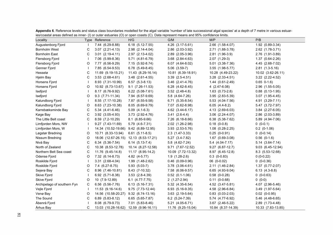
Appendix 6. Reference levels and status class boundaries modelled for the algal variable 'number of late successional algal species' at a depth of 7 metre in various estuar-ies/coastal areas defined as inner- (I) or outer estuaries (O) or open coasts (C). Data represent means and 95% confidence limits. Locality Type Reference H/G G/M M/P P/B Augustenborg Fjord I 7.44 (6.29-8.88) 6.18 (5.12-7.55) 4.26 (3.17-5.61) 2.66 (1.58-4.07) 1.92 (0.89-3.34) Bornholm West C 3.07 (2.21-4.13) 2.98 (2.14-4.04) 2.86 (2.03-3.92) 2.71 (1.88-3.78) 2.62 (1.78-3.71) Bornholm East C 3.01 (2.19-4.11) 2.97 (2.13-4.02) 2.89 (2.05-3.96) 2.81 (1.96-3.9) 2.76 (1.91-3.89) Flensborg Fjord I 7.06 (5.99-8.36) 5.71 (4.81-6.79) 3.68 (2.84-4.63) 2.07 (1.29-3) 1.37 (0.64-2.26) Flensborg Fjord O 7.77 (6.56-9.29) 7.15 (5.92-8.74) 6.07 (4.64-8.02) 5.01 (3.38-7.36) 4.45 (2.68-7.02) Genner Fjord I 7.85 (6.54-9.53) 6.78 (5.49-8.45) 5.06 (3.59-7) 3.55 (1.98-5.77) 2.81 (1.3-5.16) Hesselø C 11.69 (9.19-15.21) 11.43 (8.29-16.14) 10.81 (6.39-18.91) 10.28 (4.49-23.22) 10.02 (3.62-26.11) Hjelm Bay C 3.53 (2.68-4.61) 3.48 (2.61-4.55) 3.39 (2.5-4.51) 3.28 (2.33-4.51) 3.22 (2.22-4.52) Horsens Fjord I 8.93 (7.31-10.99) 6.57 (5.3-8.13) 3.46 (2.41-4.76) 1.44 (0.61-2.49) 0.65 0-1.6) Horsens Fjord O 10.92 (8.73-13.67) 9.1 (7.26-11.53) 6.28 (4.62-8.45) 4 (2.47-6.08) 2.96 (1.55-5.05) Isefjord I 8.17 (6.76-9.92) 6.22 (5.08-7.61) 3.52 (2.48-4.8) 1.63 (0.73-2.8) 0.88 (0.13-1.95) Isefjord O 9.3 (7.71-11.34) 7.94 (6.57-9.69) 5.8 (4.64-7.26) 3.95 (2.83-5.39) 3.07 (1.95-4.45) Kalundborg Fjord I 8.55 (7.17-10.28) 7.87 (6.55-9.58) 6.71 (5.35-8.54) 5.53 (4.04-7.56) 4.91 (3.29-7.11) Kalundborg Fjord O 8.63 (7.23-10.38) 8.05 (6.69-9.79) 7.07 (5.62-8.98) 6.05 (4.4-8.2) 5.47 (3.72-7.97) Karrebæksminde Bay C 5.34 (4.41-6.46) 5.09 (4.1-6.3) 4.62 (3.44-6.17) 4.13 (2.69-6.03) 3.84 (2.27-6.05) Køge Bay C 3.92 (3.05-4.93) 3.73 (2.92-4.76) 3.41 (2.6-4.4) 3.06 (2.24-4.07) 2.86 (2.03-3.89) The Little Belt coast C 8.59 (7.2-10.29) 8.1 (6.85-9.66) 7.26 (6.18-8.66) 6.38 (5.38-7.62) 5.89 (4.94-7.06) Limfjorden Mors, NW I 9.27 (7.43-11.69) 5.79 (4.6-7.31) 2.02 (1.26-2.98) 0.18 (0-0.8) 0 (0-0.1) Limfjorden Mors, W I 14.34 (10.52-19.66) 9.42 (6.89-12.95) 3.93 (2.53-5.76) 1.08 (0.28-2.25) 0.2 (0-1.06) Løgstør Bredning O 10.71 (8.33-13.94) 6.61 (5.11-8.5) 2.3 (1.47-3.33) 0.25 (0-0.91) 0 (0-0.14) Nissum Bredning O 18.06 (12.67-26.15) 12.13 (8.53-17.21) 5.27 (3.4-7.82) 1.67 (0.69-3.08) 0.56 (0-1.6) Nivå Bay C 6.34 (5.36-7.54) 6.14 (5.13-7.4) 5.8 (4.62-7.24) 5.4 (4.04-7.17) 5.14 (3.64-7.14) North of Zealand C 10.38 (8.53-12.78) 10.14 (8.27-12.58) 9.71 (7.67-12.52) 9.27 (6.87-12.7) 9.03 (6.45-12.94) Northern Belt Sea coast C 11.76 (9.45-14.8) 11.17 (8.95-14.2) 10.09 (7.72-13.32) 8.97 (6.45-12.8) 8.3 (5.53-12.68) Odense Fjord O 7.32 (6.14-8.73) 4.82 (4-5.77) 1.9 (1.28-2.6) 0.3 (0-0.83) 0 (0-0.22) Roskilde Fjord I 3.31 (2.68-4.04) 1.99 (1.48-2.62) 0.46 (0.09-0.96) 06 (0-0.02) 0 (0-0.36) Roskilde Fjord O 7.4 (6.27-8.75) 5.93 (5.03-7) 3.78 (3.06-4.61) 2.11 (1.46-2.84) 1.37 (0.77-2.07) Sejerø Bay C 8.96 (7.46-10.81) 8.43 (7-10.32) 7.58 (6.06-9.57) 6.65 (4.93-9.04) 6.13 (4.3-8.8) Skive Fjord I 6.92 (5.71-8.38) 3.53 (2.8-4.39) 0.52 (0.1-1.06) 0.58 (0-0.28) 0 (0-0.63) Skive Fjord O 10 (7.9-12.89) 6.1 (4.77-7.75) 2 (1.27-2.94) 0.11 (0-0.68) 0 (0-0) Archipelago of southern Fyn C 6.56 (5.56-7.76) 6.13 (5.16-7.31) 5.32 (4.35-6.54) 4.52 (3.47-5.81) 4.07 (2.96-5.46) Vejle Fjord I 11.53 (9.16-14.6) 9.75 (7.73-12.44) 6.93 (5.16-9.35) 4.58 (2.96-6.84) 3.49 (1.97-5.64) Venø Bay O 14.56 (10.58-20.27) 9.32 (6.74-13.16) 3.63 (2.19-5.64) 0.83 (0.03-2.03) 0.02 (0-0.95) The Sound C 6.89 (5.83-8.12) 6.65 (5.65-7.87) 6.2 (5.24-7.39) 5.74 (4.77-6.92) 5.46 (4.48-6.65) Åbenrå Fjord I 8.08 (6.79-9.73) 7.01 (5.83-8.46) 5.21 (4.05-6.71) 3.67 (2.46-5.22) 2.89 (1.73-4.48) Århus Bay C 13.03 (10.28-16.62) 12.59 (9.96-16.11) 11.76 (9.25-15.04) 10.84 (8.37-14.39) 10.33 (7.83-13.85)
81

Appendix 7. Modelled mean levels of total cover at a depth of 7 metre in various estuaries/coastal areas defined as inner- (I) or outer fjords (O) or open coasts (C). Data represent means and 95% confidence limits. Locality Type 2001 2003 2005 Augustenborg Fjord I 98.4 (57.1-100) 69.7 (9.5-100) Augustenborg Fjord O 81.2 (54-97.7) 63.5 (33.1-88.9) 68.3 (39.3-91.1) Bornholm West C 82.2 (51.3-99) 89 (60.9-100) 80.4 (49.6-98.4) Bornholm East C 69 (34.1-94.7) 94.9 (69.8-100) 95.1 (70.6-100) Ebeltoft C 56.4 (28.7-82) Endelave C 100 (99.8-100) Flensborg Fjord I 5.3 (0-34.4) 7.2 (0-33.3) 74.5 (27.1-99.9) Flensborg Fjord O 100 (94.1-100) 97.7 (84.4-100) 99.6 (90.7-100) Genner Fjord I 4.1 (0-43.5) 34.8 (0.8-84.7) Hesselø C 98.4 (66-100) 100 (97.6-100) 100 (89.7-100) Hjelm Bay C 89.1 (68.4-99.4) 97.9 (85.1-100) 0 (0-0) Horsens Fjord I 88.6 (57.3-100) 30 (1.6-73.7) 5.8 (0-41.9) Horsens Fjord O 96.8 (66.3-100) Isefjord I 31.7 (6.5-65.1) 92.2 (70.7-100) Isefjord O 97 (79.7-100) 99.5 (88.2-100) 100 (96-100) Kalundborg Fjord I 91.6 (71.8-99.9) 69.5 (40.5-91.8) 92.9 (72.8-100) Kalundborg Fjord O 93.7 (72.9-100) 84.9 (61-98.5) 100 (92.8-100) Karrebæksminde Bay C 99.4 (82.8-100) 99.2 (83.5-100) 95.5 (75.2-100) Kirkegrund & Knudshoved C 99.4 (89.3-100) 100 (98.2-100) 96.6 (77.2-100) Køge Bay C 12.6 (0.5-37) 50.9 (26.4-75.2) 86.2 (63.5-98.8) The Little Belt coast C 100 (96.4-100) 98.4 (89.5-100) 100 (97.8-100) Limfjorden Mors, NW I 9.3 (0-33.5) 11.9 (0.2-37.9) 14.7 (0.8-41.2) Limfjorden Mors, W I 16.6 (1.2-44.6) 17 (1.3-44.9) 10.9 (0-37.6) Løgstør Bredning O 20.9 (2.9-49.3) 23.5 (5-50) 31.6 (8.9-60.4) Nissum Bredning O 47.5 (17.3-78.8) 62.7 (31.8-88.7) 67.3 (35.9-91.9) Nivå Bay C 43 (8.6-82) 98.1 (75.4-100) 98.8 (75.8-100) North of Zealand C 100 (98.4-100) 100 (98.3-100) 100 (99.9-100) Northern Belt Sea coast C 68.3 (19.3-99.3) 86 (53.3-100) Odense Fjord O 22.1 (0-72.7) 38 (2.3-85.3) Roskilde Fjord I 11.5 (1.4-29.6) 5.3 (0-21.3) Roskilde Fjord O 99.9 (74.1-100) 95.6 (56.5-100) 95.5 (55.9-100) Sejerø Bay C 100 (96.8-100) 100 (98.8-100) 100 (99.9-100) Skive Fjord I 0 (0-10.1) 12 (0-43.1) 14.6 (0.1-47.1) Skive Fjord O 6.4 (0-34.8) 5.7 (0-32.4) 12 (0-43.4) The Great Belt coast C 97.4 (79.8-100) 77.3 (47.8-96.6) Archipelago of southern Fyn C 82.8 (53.8-98.8) Vejle Fjord I 84.5 (30.2-100) Vejle Fjord O 81.2 (51.6-98.4) 70.6 (39-93.9) 72.9 (36.3-97.1) Venø Bay O 15.2 (0-52.5) 42.1 (9.2-79.6) 26.4 (1.9-65.4) The Sound C 58.4 (36.7-78.6) 67.6 (45.6-86.1) 81.5 (60.6-95.7) Åbenrå Fjord I 100 (93.1-100) 87.1 (60.7-99.7) 100 (89-100) Åbenrå Fjord O 97.3 (80.1-100) 98.6 (78.9-100) 98.9 (82.2-100) Århus Bay C 71.3 (40.3-94) 91 (65.7-100) 47 (18.1-77.1) Århus Bay I 33.4 (8.1-65.5) 64.4 (32.7-90.3) Århus Bay O 43.5 (10-80.8) 71.6 (32.9-97.3) 66.7 (26.8-95.9)
82

Appendix 8. Modelled mean levels of cumulated cover at a depth of 7 metre in various estuaries/coastal areas defined as in-ner- (I) or outer fjords (O) or open coasts (C). Data represent means and 95% confidence limits. Locality Type 2001 2003 2005 Augustenborg Fjord I 95.4 (28.5-314) 110.3 (27.2-438.7) Augustenborg Fjord O 85.7 (43.2-169.1) 77.4 (38-156.4) 104 (52.7-204.3) Bornholm West C 97.1 (36.8-253.7) 99.7 (37.7-260.7) 90.5 (34.6-234.3) Bornholm East C 95.9 (35.4-257.4) 145.3 (54.1-387.6) 161.7 (60.7-428.1) Ebeltoft C 124.3 (60.8-253.1) Endelave C 278.4 (94.7-814.9) Flensborg Fjord I 12.8 (4.9-31.4) 23.5 (10.5-51.3) 80.1 (27.5-229.9) Flensborg Fjord O 201.3 (111.2-363.7) 133 (72.3-244) 268.3 (147.8-486.2) Genner Fjord I 22.7 (7.4-65.6) 36 (11.5-108.4) Hesselø C 246.2 (93.1-648.2) 455.4 (178.3-1160.4) 351.7 (134.1-919.5) Hjelm Bay C 143.6 (81.4-252.8) 235.7 (137.3-404.2) Horsens Fjord I 79.5 (35.4-177.1) 33.5 (12.7-85.9) 11.3 (3.8-30.9) Horsens Fjord O 120.1 (47.1-303.5) Isefjord I 40.6 (19.2-84.7) 71.3 (38.1-132.7) Isefjord O 141.7 (72.7-275.4) 167.6 (90.8-308.5) 243.9 (132.6-447.8) Kalundborg Fjord I 101.6 (56.8-181.4) 67.7 (35.7-127.8) 127.8 (69.8-233.1) Kalundborg Fjord O 136.2 (72.6-254.8) 93.9 (51.3-171.2) 150 (79.9-281.1) Karrebæksminde Bay C 173.4 (82-365.1) 195.9 (98.6-388.2) 210.2 (109.4-403.3) Kirkegrund & Knudshoved C 225.6 (129.1-393.9) 299.6 (176.4-508.5) 255.8 (130.8-499.5) Køge Bay C 8.9 (4.2-17.6) 41.9 (23.5-74.2) 112 (61.4-203.6) The Little Belt coast C 243.7 (144.8-409.9) 196.4 (116.8-329.7) 268.2 (161.9-443.7) Limfjorden Mors, NW I 13.4 (6.6-26.2) 10.9 (5.1-22.3) 12 (5.8-24.2) Limfjorden Mors, W I 21.1 (10.3-42.2) 18.8 (9.2-37.6) 14.8 (6.8-31) Løgstør Bredning O 29.1 (14.7-56.7) 19 (9.7-36.5) 30.6 (15.3-60.2) Nissum Bredning O 43.5 (21.2-88.2) 54.3 (27-108) 58.2 (28.8-116.8) Nivå Bay C 60.3 (25.5-140.9) 167.9 (77.8-360.8) 186.2 (81.4-424.5) North of Zealand C 360 (211-613.8) 360.2 (213.2-608.3) 372.3 (217.1-637.9) Northern Belt Sea coast C 199.6 (67.9-583.4) 164 (78-343.7) Odense Fjord O 55.7 (17.9-169.1) 85.4 (28.9-248.6) Roskilde Fjord I 16.7 (9.7-28.2) 9.7 (5.3-17.2) Roskilde Fjord O 164.6 (61.3-439.1) 99.7 (36.4-270) 124.8 (45.1-342.1) Sejerø Bay C 154.7 (75-318.2) 240.7 (134.2-431.2) 362.9 (195.9-671.9) Skive Fjord I 6.2 (2.3-14.7) 18.2 (8.1-39.7) 22.7 (10.2-49.4) Skive Fjord O 12.7 (5.4-28.5) 11.3 (4.8-25.1) 9.2 (3.8-20.9) The Great Belt coast C 243.5 (116.5-507.9) 177 (83.3-375) Archipelago of southern Fyn C 127.1 (49.4-324.4) Vejle Fjord I 76.7 (22.9-251.9) Vejle Fjord O 125.9 (61.4-257.2) 59.5 (30-117) 65.4 (23.2-180.9) Venø Bay O 36.6 (15.3-86) 46 (19.3-107.7) 29.5 (12.1-70.1) The Sound C 97.2 (58.2-161.9) 118.5 (70.5-198.6) 64.4 (37.1-111.3) Åbenrå Fjord I 218.1 (109.8-432.4) 149.8 (74.4-300.8) 252.4 (123.6-514.3) Åbenrå Fjord O 147.6 (75-289.3) 152.7 (68.8-337.7) 191.9 (91.9-399.7) Århus Bay C 164 (76.7-349.7) 174 (80.8-373.2) 72.4 (33.7-154.5) Århus Bay I 127.4 (58.5-276.2) 104.6 (48.3-225.4)
83

Appendix 9. Modelled mean levels of cover of late successionals at a depth of 7 metre in various estuaries/coastal areas de-fined as inner- (I) or outer estuaries (O) or open coasts (C). Data represent means and 95% confidence limits. Locality Type 2001 2003 2005
Augustenborg Fjord I 135.4 (23-776.1) 130.8 (16.8-977.2)
Augustenborg Fjord O 95.2 (39.2-229) 62.1 (24.4-156.1) 52.3 (21.3-126.1) Bornholm West C 25.2 (8.8-68.7) 25.6 (9-69.9) 27.1 (9.8-72.2)
Bornholm East C 29.7 (9.9-85.8) 33.4 (11.3-95.7) 55.8 (19.5-156.2)
Ebeltoft C 93.5 (40.3-215.3) Endelave C 248.3 (70.4-869.4)
Flensborg Fjord I 2.3 (0-9.7) 6.6 (1.8-19.9) 18.7 (3.6-83.9)
Flensborg Fjord O 166 (80.4-341.6) 93.7 (44-198.1) 169.6 (81.5-351.9) Genner Fjord I 18.6 (3.3-89.7) 34 (6.1-172.2)
Hesselø C 133.7 (29.8-587.1) 182.9 (42.5-775.8) 142 (32-618.4)
Hjelm Bay C 32.4 (14.4-71.2) 51.3 (23.9-108.5) Horsens Fjord I 71.7 (23.6-214.4) 20.8 (4.7-82.3) 5.8 (0.7-25.7)
Horsens Fjord O 106.6 (28.2-395.9)
Isefjord I 5.7 (1.4-17.3) 25.2 (10.1-60.5) Isefjord O 110.3 (46.1-262.2) 108.9 (46.8-251.4) 110.1 (47.1-255.7)
Kalundborg Fjord I 21.5 (9.2-48.4) 18.7 (7.2-46.1) 39.5 (16.7-91.6)
Kalundborg Fjord O 47.3 (19.3-114) 29 (12.3-66.8) 86.4 (35.3-209.4) Karrebæksminde Bay C 116.5 (40.2-333.8) 65 (24.1-172.9) 71 (28-177.8)
Kirkegrund & Knudshoved C 50.1 (22.8-108.7) 105.9 (50.5-220.8) 46 (17.7-117.2)
Køge Bay C 3.2 (0.8-8.9) 2.6 (0.7-6.6) 6.2 (2.2-14.9) The Little Belt coast C 197.3 (107.6-360.9) 137.1 (75-250.1) 193.1 (108.4-343.3)
Limfjorden Mors, NW I 20.7 (7.7-53.2) 9.7 (3.3-25.7) 8.8 (3-23)
Limfjorden Mors, W I 11.5 (3.9-30.4) 18.1 (6.6-46.8) 11.9 (4-32.5) Løgstør Bredning O 43.3 (17-107.9) 20.6 (8.4-48.2) 26.9 (10.8-65.4)
Nissum Bredning O 73.7 (26.9-198.8) 74.2 (28.7-189.4) 79 (30.1-204.9)
Nivå Bay C 3.1 (0.2-13.1) 27 (8.1-85.2) 35 (9.9-118.7) North of Zealand C 159.3 (75.6-334.7) 151.2 (72.8-312.9) 143.3 (67.3-303.8)
Northern Belt Sea coast C 124.5 (26.1-580.5) 97.2 (31.8-292.5)
Odense Fjord O 57.2 (11.1-279.8) 74.3 (15.5-343.7) Roskilde Fjord I -0.4 (-0.7-0.3) -0.5 (-0.8-0)
Roskilde Fjord O 101.6 (21.9-458.6) 86.3 (18.2-396.6) 10.8 (1.6-53.4)
Sejerø Bay C 119.4 (42.6-331.2) 167.3 (75.3-370.7) 212 (88.1-507.8) Skive Fjord I 6.9 (1.5-23.8) 6.1 (1.4-19.9) 7.8 (2-24.8)
Skive Fjord O 23.9 (7.1-75) 9.1 (2.4-28.9) 6.5 (1.5-21.2)
The Great Belt coast C 221.4 (90.6-538.7) 134.1 (53.3-335.1) Archipelago of southern Fyn C 83.2 (32.4-211.3)
Vejle Fjord I 96.4 (16.2-550.3)
Vejle Fjord O 102 (39.1-263.8) 38.6 (14.2-102.3) 74.4 (24.1-225.4) Venø Bay O 75.9 (21.8-259.1) 45.7 (13.4-150.4) 29.9 (8.4-100.5)
The Sound C 31.8 (16.2-61.5) 29 (14.6-56.9) 51.5 (25.3-103.9)
Åbenrå Fjord I 169.7 (68.6-417.5) 97.6 (38.5-245.2) 185.1 (71.6-475.7) Åbenrå Fjord O 112.8 (46.4-272.5) 117.1 (39.7-341.5) 152.1 (56.8-404.3)
Århus Bay C 125.4 (48.7-320.1) 143 (55.1-368.9) 56.3 (21.7-143.8)
Århus Bay I 107.5 (40.6-282) 75.8 (28.8-196.9) Århus Bay O 125 (37.9-406.6) 112.7 (34.2-366.4) 57.1 (16.3-194.5)
84

Appendix 10. Modelled mean levels of cover of opportunists at a depth of 7 metre in various estuaries/coastal areas defined as inner- (I) or outer estuaries (O) or open coasts (C). Data represent means and 95% confidence limits. Locality Type 2001 2003 2005 Augustenborg Fjord I 1.2 (-0.6-10.4) 2 (-0.5-19.6) Augustenborg Fjord O 3.7 (0.7-12.2) 1.9 (0-7.5) 16.6 (5.3-48.3) Bornholm West C 39.6 (5.3-260.7) 49.4 (6.8-324.6) 32.3 (4.2-211.7) Bornholm East C 21.5 (2.4-147.7) 54 (7.4-360.3) 52.6 (7.2-348.6) Ebeltoft C 9.3 (2.3-30.7) Endelave C 24.1 (2.5-177.2) Flensborg Fjord I 1.6 (-0.3-8.1) 2.6 (0.1-10.1) 14.4 (2.4-68.7) Flensborg Fjord O 13.2 (4.5-35.4) 10 (3.2-27.6) 24.9 (9.1-65.7) Genner Fjord I 0.2 (-0.7-4) 5.6 (0.5-28.1) Hesselø C 70.3 (19-253.2) 274.4 (80.2-933.1) 131.1 (36.3-466.4) Hjelm Bay C 70.1 (29.5-164.7) 138.1 (60.9-311.9) Horsens Fjord I 4.3 (0.7-16.2) 9.9 (2-38.8) 7.5 (1.2-31.5) Horsens Fjord O 7.4 (1.2-30.3) Isefjord I 40.6 (13.6-117.3) 44.5 (17.4-111.5) Isefjord O 14.2 (4.5-40.9) 63.8 (25.2-159.2) 153.5 (61.6-379.9) Kalundborg Fjord I 95.2 (39.8-226.1) 71.8 (28.1-181) 82.8 (33.3-203.4) Kalundborg Fjord O 106.6 (42.4-266) 76.3 (30.9-186.2) 65 (25.6-163) Karrebæksminde Bay C 38.9 (12.6-116.3) 115.4 (42.3-312.4) 202.1 (78.2-520) Kirkegrund & Knudshoved C 110.6 (47.4-256.3) 145.6 (65.3-323.3) 272 (101.2-727.8) Køge Bay C 9.1 (2.9-24.9) 58.1 (24.4-136.8) 72 (28.8-177.8) The Little Belt coast C 7.9 (2.8-20.2) 13 (4.9-32.2) 18.4 (7.4-44) Limfjorden Mors, NW I 1.7 (0.1-5.9) 1.4 (-0.1-5.6) 2.5 (0.3-8.4) Limfjorden Mors, W I 4 (0.8-12.8) 2 (0.1-7.2) 1.7 (-0.1-7.1) Løgstør Bredning O 0.5 (-0.4-2.8) 1.9 (0.1-6.7) 4.2 (0.8-13.6) Nissum Bredning O 3.1 (0.5-10.2) 3.3 (0.5-11) 2.6 (0.3-9.2) Nivå Bay C 77.3 (23.5-249.1) 159.4 (54.8-460.2) 130.1 (40.8-410.4) North of Zealand C 106.3 (47.3-237.2) 127.3 (57.5-280.3) 229.2 (102.1-512.6) Northern Belt Sea coast C 30.2 (6-137.7) 60.4 (21.2-168.9) Odense Fjord O 5.9 (0.5-30.8) 15.3 (2.7-70.5) Roskilde Fjord I 25.8 (11.4-56.9) 11.9 (4.7-27.9) Roskilde Fjord O 36.7 (9.4-135.6) 14.6 (3.2-56.5) 44.4 (11-171) Sejerø Bay C 13.4 (4.1-39.6) 58 (23.8-139.2) 110.4 (44.4-272.2) Skive Fjord I 1.2 (-0.2-5.6) 3.9 (0.6-13.6) 4.7 (0.9-16) Skive Fjord O -0.4 (-0.8-0.8) 1.5 (-0.2-6.4) 1.4 (-0.2-6.1) The Great Belt coast C 18.2 (5.1-60) 16.6 (4.5-55.9) Archipelago of southern Fyn C 30.6 (4-199.6) Vejle Fjord I 0.4 (-0.7-6.2) Vejle Fjord O 4.8 (1-15.8) 15.6 (5.4-42.4) 1.3 (-0.7-14.3) Venø Bay O -0.3 (-0.8-1.1) 2.9 (0.1-12.2) 3 (0.2-12.7) The Sound C 50.1 (22.1-112.1) 99.8 (44.2-223.9) 22.3 (9-53.1) Åbenrå Fjord I 17.5 (5.6-51.3) 12.1 (3.6-36.6) 69.7 (23.2-206.2) Åbenrå Fjord O 12.2 (3.7-35.6) 10.4 (2.5-36.2) 43.1 (13.6-131.9) Århus Bay C 16.7 (4.5-56.2) 17 (4.5-57.3) 7.5 (1.6-26.3) Århus Bay I 11.1 (2.7-38.8) 13.6 (3.5-46.5) Århus Bay O 17.9 (4.2-67.9) 22.3 (5.4-83.8) 23.2 (5.4-90.2)
85

Appendix 11. Modelled mean levels of fraction of opportunists at a depth of 7 metre in various estuaries/coastal areas defined as inner- (I) or outer fjords (O) or open coasts (C). Data represent means and 95% confidence limits. Locality Type 2001 2003 2005 Augustenborg Fjord I 0.8 (0-28.1) 0.4 (0-34.1) Augustenborg Fjord O 7.2 (0-25.2) 6.5 (0-25) 34.7 (13.6-59.7) Bornholm West C 60.6 (28.3-88.5) 63 (30.5-90) 54.1 (23-83.5) Bornholm East C 39.5 (10.8-72.9) 57.7 (24.8-87.2) 45.8 (15.5-77.9) Ebeltoft C 14.2 (1.6-36.3) Endelave C 9 (0-40.4) Flensborg Fjord I 66.5 (33.5-92.3) 50.2 (22.4-77.9) 57.2 (17.6-91.9) Flensborg Fjord O 13 (2.3-30.5) 17.3 (4.2-36.9) 22.1 (7.1-42.3) Genner Fjord I 17.7 (0.1-54.9) 47.6 (10.8-86.1) Hesselø C 20.1 (0.8-55.4) 44.5 (13-78.7) 28.6 (3.7-64.9) Hjelm Bay C 47.3 (26.6-68.5) 52.7 (32.5-72.4) Horsens Fjord I 9.1 (0-33.1) 19.6 (0.7-55) 37 (7-74.4) Horsens Fjord O 11.5 (0-42.2) Isefjord I 89.9 (67.3-99.9) 63.6 (39.7-84.3) Isefjord O 13.4 (1.5-34.5) 22.9 (6.7-45.1) 44.5 (22.4-67.8) Kalundborg Fjord I 72.7 (51.5-89.5) 69.9 (46.3-88.9) 59.3 (36.2-80.4) Kalundborg Fjord O 59.1 (35.4-80.7) 61.6 (39-81.9) 37.4 (16.4-61.2) Karrebæksminde Bay C 10.6 (0.1-34.8) 47.5 (22.1-73.5) 63.1 (38.2-84.7) Kirkegrund & Knudshoved C 47.4 (27-68.4) 42.1 (23.4-62) 78.7 (54.2-95.4) Køge Bay C 47.6 (24-71.7) 96.4 (84.4-100) 92.9 (76.9-99.8) The Little Belt coast C 6.6 (0.5-18.9) 14.3 (3.9-29.6) 14.7 (4.4-29.6) Limfjorden Mors, NW I 30.3 (10.8-54.4) 36.1 (14.5-61.3) 49.5 (25.8-73.4) Limfjorden Mors, W I 46.2 (22.3-71) 25 (7.1-49.1) 41.8 (17.6-68.3) Løgstør Bredning O 4.4 (0-20.1) 10.8 (1-29.2) 26.3 (8.1-50.2) Nissum Bredning O 11.7 (0.6-33.8) 3.3 (0-18.2) 3 (0-17.8) Nivå Bay C 92.9 (67.8-100) 72.9 (44-93.9) 58.8 (27.3-86.8) North of Zealand C 26.8 (11.2-46.1) 32.9 (16.1-52.4) 47.3 (27.6-67.5) Northern Belt Sea coast C 31.1 (3.4-70.7) 29.1 (7.9-57) Odense Fjord O 11 (0-47.5) 21.8 (0.7-60.4) Roskilde Fjord I 0 (0-0) 100 (98.1-100) 100 (99.3-100) Roskilde Fjord O 18.4 (0.4-54) 9.1 (0-40.9) 70.4 (32-96.8) Sejerø Bay C 9.3 (0.1-31.3) 19.2 (5.3-39.2) 24.9 (7.8-47.6) Skive Fjord I 55.5 (25.9-83.1) 58.3 (30.1-83.8) 55.7 (27.7-81.8) Skive Fjord O 8.5 (0-31.4) 36.2 (12.2-64.6) 52.3 (24.6-79.3) The Great Belt coast C 13.2 (1-35.9) 19.1 (3-44.5) Archipelago of southern Fyn C 28.2 (5.6-59.5) Vejle Fjord I 0 (0-19.8) Vejle Fjord O 8.2 (0-28.3) 16.9 (2.6-40.1) 0.2 (0-15.5) Venø Bay O 0.2 (0-13.6) 7.8 (0-32.6) 14.7 (0.4-43.6) The Sound C 47.1 (28.6-66) 64.1 (44.7-81.3) 45.9 (25.9-66.6) Åbenrå Fjord I 16.9 (2.7-39.6) 20.1 (4-44.2) 33.2 (11.4-59.9) Åbenrå Fjord O 19.3 (4.1-42.1) 12.5 (0.3-38.6) 28.7 (7.9-56.1) Århus Bay C 20.3 (3.5-46.2) 18.4 (2.6-44.1) 16.9 (2.1-41.6) Århus Bay I 13.8 (0.9-38.3) 23.7 (5-50.6) Århus Bay O 23.1 (2.9-54.5) 27.9 (5-60) 48.2 (17-80.2)
86

Appendix 12. Modelled mean levels of number of perennials at a depth of 7 metre in various estuaries/coastal areas defined as inner- (I) or outer fjords (O) or open coasts (C). Data represent means and 95% confidence limits. Locality Type 2001 2003 2005 Augustenborg Fjord I 5.7 (2.6-11.5) 7.7 (3.1-17.5) Augustenborg Fjord O 6.1 (4.3-8.5) 5.3 (3.6-7.6) 5.2 (3.7-7.2) Bornholm West C 2.3 (1.5-3.3) 2.6 (1.7-3.8) 2.4 (1.6-3.3) Bornholm East C 2.3 (1.4-3.5) 2.7 (1.7-4) 3.1 (2-4.4) Ebeltoft C 8.2 (6.3-10.6) Endelave C 5.6 (3.5-8.7) Flensborg Fjord I 0.9 (0.3-1.9) 1.9 (1-3.1) 1.8 (0.6-3.9) Flensborg Fjord O 7.9 (6.1-10) 5.8 (4.4-7.6) 6.6 (5.1-8.5) Genner Fjord I 2.2 (0.9-4.3) 3.3 (1.4-6.5) Hesselø C 10.8 (6.2-18.2) 12.4 (7.3-20.7) 11.2 (6.5-18.8) Hjelm Bay C 4.3 (3.1-5.8) 4.8 (3.6-6.4) Horsens Fjord I 6.7 (4.3-10.2) 6.1 (3.3-10.7) 2.2 (0.9-4.3) Horsens Fjord O 9.1 (5.4-15.1) Isefjord I 1.2 (0.5-2.1) 4.5 (3.1-6.3) Isefjord O 3.6 (2.5-5.1) 5.4 (3.8-7.5) 6.1 (4.3-8.6) Kalundborg Fjord I 5 (3.7-6.8) 4.2 (3-5.9) 6.3 (4.5-8.6) Kalundborg Fjord O 6.9 (4.9-9.4) 5.1 (3.7-6.9) 9.5 (6.9-13) Karrebæksminde Bay C 2.6 (1.5-4.3) 3.8 (2.4-5.7) 5.6 (3.9-7.9) Kirkegrund & Knudshoved C 6.2 (4.7-8.3) 9.4 (7.2-12.2) 7.5 (5.2-10.7) Køge Bay C 0.9 (0.4-1.6) 0.7 (0.4-1.2) 2.6 (1.8-3.6) The Little Belt coast C 8.2 (6.7-10.1) 8.2 (6.7-10) 8.8 (7.3-10.6) Limfjorden Mors, NW I 2.9 (1.9-4.3) 2.4 (1.5-3.5) 2 (1.3-3.1) Limfjorden Mors, W I 3 (2-4.5) 2.7 (1.7-4) 1.3 (0.7-2.2) Løgstør Bredning O 3.8 (2.6-5.4) 2.7 (1.8-3.8) 1.4 (0.8-2.2) Nissum Bredning O 6.5 (4.5-9.3) 7.1 (5-10) 6.6 (4.6-9.5) Nivå Bay C 2.8 (1.5-4.9) 4.6 (2.8-7.3) 5.5 (3.3-8.9) North of Zealand C 11.5 (8.8-14.9) 11.7 (9.1-15) 11.3 (8.7-14.8) Northern Belt Sea coast C 10.3 (5.9-17.6) 8.1 (5.3-12.2) Odense Fjord O 8.3 (4.5-14.6) 13.3 (7.8-22.4) Roskilde Fjord I 0.4 (0.1-0.7) 0.3 (0-0.6) Roskilde Fjord O 3.2 (1.5-6) 2.6 (1.2-5.1) 0.7 (0-1.8) Sejerø Bay C 8.7 (5.8-12.8) 8.5 (6.4-11.1) 12.7 (9.1-17.5) Skive Fjord I 0.8 (0.2-1.7) 1 (0.4-1.8) 0.9 (0.3-1.7) Skive Fjord O 2.9 (1.7-4.6) 2.5 (1.5-4) 1.7 (0.9-2.8) The Great Belt coast C 15.1 (11.4-19.8) 12 (8.9-16.1) Archipelago of southern Fyn C 4.3 (3.2-5.8) Vejle Fjord I 8.1 (3.9-15.9) Vejle Fjord O 8.2 (5.7-11.5) 7.4 (5-10.7) 8 (5.5-11.6) Venø Bay O 5.4 (3.2-8.7) 6 (3.7-9.4) 2.6 (1.4-4.4) The Sound C 3.7 (2.9-4.7) 3.3 (2.6-4.3) 5.7 (4.5-7.3) Åbenrå Fjord I 7.1 (5.1-9.9) 6.6 (4.6-9.3) 8 (5.6-11.3) Åbenrå Fjord O 8.3 (6-11.3) 10.6 (6.9-15.8) 10.6 (7.4-15.2) Århus Bay C 11.7 (8.6-15.6) 11.3 (8.3-15.3) 8.1 (5.9-10.9) Århus Bay I 9.5 (6.9-13) 9 (6.5-12.2) Århus Bay O 13.6 (9.1-20.1) 10 (6.6-14.9) 7.5 (4.7-11.5)
87

Appendix 13. Results of power analyses showing the least number (n) of observations necessary to evaluate environmental status based on the algal variable 'total cover' in 'face value' and 'fail safe' classification scenarios with a standard power value of 80%. Results are shown for all areas which fulfilled the power requirements within combinations of 1-3 divers, 1-10 sites and 2-10 point samples per site. Type indicates inner fjords (I), outer fjords (O) and open coast (C). Face value Fail safe Area Type n total n diver n site n sample n total n diver n site n sample Augustenborg Fjord I 8 2 2 2 Flensborg Fjord I 6 1 2 3 Genner Fjord I 24 2 6 2 Horsens Fjord I 3 1 1 3 24 2 6 2 Horsens Fjord O 12 1 6 2 Isefjord I 3 1 1 3 42 3 7 2 Isefjord O 16 2 4 2 Limfjorden Mors, NW I 2 1 1 2 4 1 1 4 Limfjorden Mors, W I 2 1 1 2 6 1 2 3 Løgstør Bredning O 2 1 1 2 3 1 1 3 Nissum Bredning O 2 1 1 2 6 1 3 2 Odense Fjord O 2 1 1 2 6 1 2 3 Roskilde Fjord I 2 1 1 2 4 1 1 4 Roskilde Fjord O 6 1 2 3 Skive Fjord I 2 1 1 2 2 1 1 2 Skive Fjord O 2 1 1 2 3 1 1 3 Vejle Fjord I 12 2 3 2 Venø Bay O 2 1 1 2 4 1 2 2 Åbenrå Fjord I 24 2 6 2
Appendix 14. Results of power analyses showing the least number (n) of observations necessary to evaluate environmental status based on the algal variable 'cumulated cover' in 'face value' and 'fail safe' classification scenarios with a standard power value of 80%. Results are shown for all areas which fulfilled the power requirements within combinations of 1-3 divers, 1-10 sites and 2-10 point samples per site. Type indicates inner fjords (I), outer fjords (O) and open coast (C). Face value Fail safe Area Type n total n diver n site n sample n total n diver n site n sample Limfjorden Mors, NW I 18 3 3 2 Limfjorden Mors, W I 48 3 8 2 Løgstør Bredning O 18 3 3 2 Odense Fjord O 60 3 10 2 Roskilde Fjord I 24 3 4 2 Skive Fjord I 4 1 2 2 Skive Fjord O 16 2 4 2 Venø Bay O 30 3 5 2
88
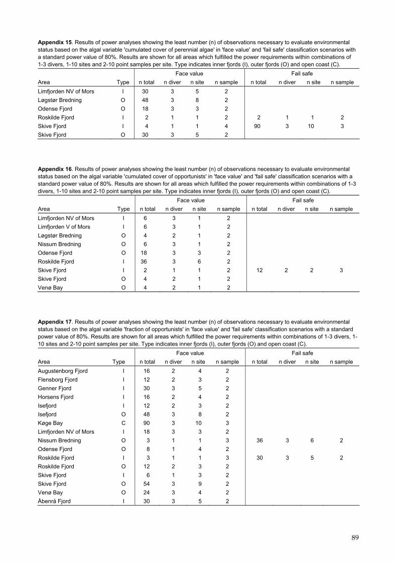
Appendix 15. Results of power analyses showing the least number (n) of observations necessary to evaluate environmental status based on the algal variable 'cumulated cover of perennial algae' in 'face value' and 'fail safe' classification scenarios with a standard power value of 80%. Results are shown for all areas which fulfilled the power requirements within combinations of 1-3 divers, 1-10 sites and 2-10 point samples per site. Type indicates inner fjords (I), outer fjords (O) and open coast (C). Face value Fail safe Area Type n total n diver n site n sample n total n diver n site n sample Limfjorden NV of Mors I 30 3 5 2 Løgstør Bredning O 48 3 8 2 Odense Fjord O 18 3 3 2 Roskilde Fjord I 2 1 1 2 2 1 1 2 Skive Fjord I 4 1 1 4 90 3 10 3 Skive Fjord O 30 3 5 2
Appendix 16. Results of power analyses showing the least number (n) of observations necessary to evaluate environmental status based on the algal variable 'cumulated cover of opportunists' in 'face value' and 'fail safe' classification scenarios with a standard power value of 80%. Results are shown for all areas which fulfilled the power requirements within combinations of 1-3 divers, 1-10 sites and 2-10 point samples per site. Type indicates inner fjords (I), outer fjords (O) and open coast (C). Face value Fail safe Area Type n total n diver n site n sample n total n diver n site n sample Limfjorden NV of Mors I 6 3 1 2 Limfjorden V of Mors I 6 3 1 2 Løgstør Bredning O 4 2 1 2 Nissum Bredning O 6 3 1 2 Odense Fjord O 18 3 3 2 Roskilde Fjord I 36 3 6 2 Skive Fjord I 2 1 1 2 12 2 2 3 Skive Fjord O 4 2 1 2 Venø Bay O 4 2 1 2
Appendix 17. Results of power analyses showing the least number (n) of observations necessary to evaluate environmental status based on the algal variable 'fraction of opportunists' in 'face value' and 'fail safe' classification scenarios with a standard power value of 80%. Results are shown for all areas which fulfilled the power requirements within combinations of 1-3 divers, 1-10 sites and 2-10 point samples per site. Type indicates inner fjords (I), outer fjords (O) and open coast (C). Face value Fail safe Area Type n total n diver n site n sample n total n diver n site n sample Augustenborg Fjord I 16 2 4 2 Flensborg Fjord I 12 2 3 2 Genner Fjord I 30 3 5 2 Horsens Fjord I 16 2 4 2 Isefjord I 12 2 3 2 Isefjord O 48 3 8 2 Køge Bay C 90 3 10 3 Limfjorden NV of Mors I 18 3 3 2 Nissum Bredning O 3 1 1 3 36 3 6 2 Odense Fjord O 8 1 4 2 Roskilde Fjord I 3 1 1 3 30 3 5 2 Roskilde Fjord O 12 2 3 2 Skive Fjord I 6 1 3 2 Skive Fjord O 54 3 9 2 Venø Bay O 24 3 4 2 Åbenrå Fjord I 30 3 5 2
89
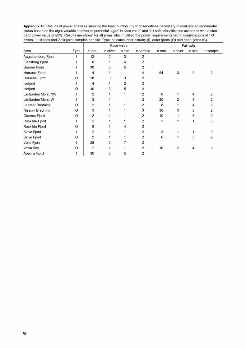
90
Appendix 18. Results of power analyses showing the least number (n) of observations necessary to evaluate environmental status based on the algal variable 'number of perennial algae' in 'face value' and 'fail safe' classification scenarios with a stan-dard power value of 80%. Results are shown for all areas which fulfilled the power requirements within combinations of 1-3 divers, 1-10 sites and 2-10 point samples per site. Type indicates inner estuary (I), outer fjords (O) and open fjords (C). Face value Fail safe Area Type n total n diver n site n sample n total n diver n site n sample Augustenborg Fjord I 12 2 3 2 Flensborg Fjord I 8 1 4 2 Genner Fjord I 30 3 5 2 Horsens Fjord I 4 1 1 4 54 3 9 2 Horsens Fjord O 18 3 3 2 Isefjord I 4 1 2 2 Isefjord O 30 3 5 2 Limfjorden Mors, NW I 2 1 1 2 8 1 4 2 Limfjorden Mors, W I 3 1 1 3 20 2 5 2 Løgstør Bredning O 2 1 1 2 8 1 4 2 Nissum Bredning O 3 1 1 3 36 3 6 2 Odense Fjord O 2 1 1 2 10 1 5 2 Roskilde Fjord I 2 1 1 2 3 1 1 3 Roskilde Fjord O 8 1 4 2 Skive Fjord I 2 1 1 2 3 1 1 3 Skive Fjord O 2 1 1 2 6 1 3 2 Vejle Fjord I 28 2 7 2 Venø Bay O 2 1 1 2 16 2 4 2 Åbenrå Fjord I 30 3 5 2

National Environmental Research Institute, NERI, is a part of
University of Aarhus.
NERI’s tasks are primarily to conduct research, collect data, and give advice
on problems related to the environment and nature.
At NERI’s website www.neri.dk you’ll fi nd information regarding ongoing research and development projects.
Furthermore the website contains a database of publications including scientifi c articles, reports, conference contributions etc. produced by NERI staff members.
National Environmental Research InstituteDanmarks Miljøundersøgelser
NERIDMU
Further information: www.neri.dk
National Environmental Research Institute Management Frederiksborgvej 399 Personnel and Economy Secretariat PO Box 358 Monitoring, Advice and Research Secretariat DK-4000 Roskilde Department of Policy Analysis Denmark Department of Atmospheric Environ ment Tel: +45 4630 1200 Department of Marine Ecology Fax: +45 4630 1114 Department of Environmental Chemistry and Microbiology Department of Arctic Environment
National Environmental Research Institute Monitoring, Advice and Research Secretariat Vejlsøvej 25 Department of Marine Ecology PO Box 314 Department of Terrestrial Ecology DK-8600 Silkeborg Department of Freshwater Ecology Denmark Tel: +45 8920 1400 Fax: +45 8920 1414
National Environmental Research Institute Department of Wildlife Ecology and Biodiversity Grenåvej 14, Kalø DK-8410 Rønde Denmark Tel: +45 8920 1700 Fax: +45 8920 1514

NERI Technical Reports
NERI’s website www.neri.dk contains a list of all published technical reports along with other NERI publications. All recent reports can be downloaded in electronic format (pdf) without charge. Some of the Danish reports include an English summary.
Nr./No. 2008
Nr. 676 Fodring af kortnæbbede gæs om foråret i Vestjylland. Biologiske fakta til understøttelse af fremtidig forvaltningsstrategi. Af Madsen, J. 20 s. (elektronisk)
675 Annual Danish Emission Inventory Report to UNECE. Inventories from the base year of the protocols to year 2006. By Nielsen, O.-K. et al. 504 pp. (electronic)
674 Environmental monitoring at the cryolite mine in Ivittuut, Spouth Greenland, in 2007. Johansen, P. et al. 31 pp. (electronic)
672 Revised emission factors for gas engines including start/stop emissions. Sub-report 3 (NERI). By Nielsen, M., Illerup, J.B. & Birr-Petersen, K. 67 pp. (electronic)
671 DEVANO. Decentral Vand- og Naturovervågning. Programbeskrivelse 2008. Af Boutrup, S. & Jensen, P.N. (red.). 33 s. (elektronisk)
670 Prioriteringsmetoder i forvaltningen af Habitatdirektivets naturtyper og arter i Natura 2000-områder. Af Skov, F. et al. 36 s. (elektronisk)
669 Identifi kation af referencevandløb til implementering af vandrammedirektivet i Danmark. Kristensen, E.A. et al. 55 s. elektronisk)
668 Brændefyring i hjemmet – praksis, holdninger og regulering. Af Petersen, L.K. & Martinsen, L. 48 s. (elektronisk)
667 Denmark’s National Inventory Report 2008. Emission Inventories 1990-2006 – Submitted under the United Nations Framework Convention on Climate Change. By Nielsen, O.-K. et al. 701 pp. (electronic)
666 Agerhønens biologi og bestandsregulering. En gennemgang af den nuværende viden. Af Kahlert, T., Asferg, T. & Odderskær, P. 61 s.
665 Individual traffi c-related air pollution and new onset adult asthma. A GIS-based pilot study. By Hansen, C.L. et al. 23 pp.
664 Aluminiumsmelter og vandkraft i det centrale Grønland. Datagrundlag for natur og ressourceudnyttelse i forbindelse med udarbejdelse af en Strategisk Miljøvurdering (SMV). Af Johansen, P. et al. 110 s.
663 Tools to assess conservation status on open water reefs in Nature-2000 areas. By Dahl, K. & Carstensen, J. 25 pp.
662 Environmental monitoring at the Nalunaq Gold Mine, South Greenland, 2007. By Glahder, C.M., Asmund, G. & Riget, F. 31 pp.
661 Tilstandsvurdering af levesteder for arter. Af Søgaard, B. et al. 72 s.
660 Opdatering af vurdering af anvendelse af SCR-katalysatorer på tunge køretøjer som virkemiddel til nedbringelse af NO2 forureningen i de største danske byer. Af Ketzel, M. & Palmgren, F. 37 s.
659 Optimering af behandlingseffekten i akvakultur. Minimering af forbrug og udlednbing af hjælpestoffer. Af Sortkjær, O. et al. 124 s. (also available in print edtion).
658 Danske kystklitter – vegetation og jordbundskemi. Analyse af NOVANA-data 2004-2006. Af Damgaard, C., Nygaard, B. & Nielsen, K.E. 66 s.
657 High density areas for harbour porpoises in Danish waters. By Teilmann, J. et al. 40 pp.
656 Manglende indberetninger til vildtudbyttestatistikken i jagtsæsonen 2006/07. Af Asferg, T. 21 s.
654 Rapportering af Luftemissioner på Grid. Metoder og principper. Af Jensen, M.T. et al. 56 s.
653 Control of Pesticides 2006. Chemical Substances and Chemical Preparations. By Krongaard, T., Petersen, K.K. & Christoffersen, C. 25 pp.
652 A preliminary strategic environmental impact assessment of mineral and hydrocarbon activities on the Nuussuaq peninsula, West Greenland. By Boertmann, D. et al. 66 pp.
651 Undersøgelser af jordhandler i forbindelse med naturgenopretning. Af Jensen, P.L., Schou, J.S. & Ørby, P.V. 44 s.
650 Fuel consumption and emissions from navigation in Denmark from 1990-2005 – and projections from 2006-2030. By Winther, M. 108 pp.

[Blank page]

National Environmental Research Institute 978-87-7073-060-0University of Aarhus . Denmark ISSN 1600-0048
This report contributes to the development of tools that can be applied to assess the five classes of ecological status of the Water Framework Di-rective based on the biological quality elements phytoplankton and ma-croalgae. Nitrogen inputs and concentrations representing reference conditions and boundaries between the five ecological status classes were calculated from estimates of nitrogen inputs from Denmark to the Danish straits since 1900 combined with expert judgement of the general environ-mental conditions of Danish waters during different time periods. From these calculated nitrogen concentrations and a macroalgal model ecolo-gical status class boundaries were established for six macroalgal indica-tors in a number of Danish estuaries and coastal areas. Furthermore, site- specific correlations between concentrations of nitrogen and chlorophyll a were used to define reference conditions and ecological status class bound-aries for the phytoplankton metric ‘mean summer concentration of chloro- phyll a’ in several Danish estuaries and coastal areas. Precision of the two different chlorophyll a indicators ‘summer mean’ and ‘90-percentile’ was evaluated. The 90-percentile was substantially more uncertain than the mean or median indicators, particularly for small sample sizes but also for large sample sizes.
683 M
acroalg
ea and
ph
ytop
lankto
n as in
dicato
rs of eco
log
ical status
of D
anish
coastal w
aters