J . Fluid Mvch (1993), uol. 248. p p . 637-661 Copyright 0 1993 Cambridge University Press

637

Mach reflection of a large-amplitude solitary wave

By MITSUHIRO TANAKA Department of Applied Mathematics. Faculty of Engineering, Gifu IJniversity, 1-1 Yanagido,

Gifu, 501-11 Japan

(Received 6 April 1992 and in revised form 21 October 1992)

Reflection of an obliquely incident solitary wave by a vertical wall is studied numerically by applying the ‘ high-order spectral method ’ developed by Dom- mermuth & Yue (1987). According to the analysis by Miles (1977a, b ) which is valid when ai < 1, the regular type of reflection gives way to ‘Mach reflection’ when $,/(3a,)i < 1, where a, is the amplitude of the incident wave divided by the quiescent water depth d and $i is the angle of incidence. I n Mach reflection, the apex of the incident and the reflected waves moves away from the wall a t a constant angle ($*) say), and is joined to the wall by a third solitary wave called ‘Mach stem’. Miles model predicts that the amplitude of Mach stem, and so the run-up at the wall, is hi when = ( 3 4 ; .

Our numerical results shows, however, that the effect of large amplitude tends to prevent the Mach reflection to occur. Even when the Mach reflection occurs, it is ‘contaminated’ by regular reflection in the sense that all the important quantities that characterize the reflection pattern, such as the stem angle $*, the angle of reflection k,, and the amplitude of the reflected wave a,, are all shifted from the values predicted by Miles’ theory toward those corresponding to the regular reflection, i.e. $* = 0, $, = and a, = a,. According to our calculations for a, = 0.3, the changeover from Mach reflection to regular reflection happens at $, z 37.8”, which is much smaller than ( 3 4 4 = 54.4’, and the highest Mach stem is observed for $i = 35” ($,/(3ai); = 0.644). Although the ‘four-fold amplification’ is not observed for any value of $, considered here, it is found that the Mach stem can become higher than the highest two-dimensional steady solitary wave for the prescribed water depth. The numerical result is also compared with the analysis by Johnson (1982) for the oblique interaction between one large and one small solitary wave, which shows much better agreement with the numerical result than the Miles’ analysis does when $, is sufficiently small and the Mach reflection occurs.

1. Introduction The problem of oblique incidence of a solitary wave with small wave height (ai 4

1) on a vertical wall was studied theoretically by Miles (1977a) b ) as a special case of oblique interaction of two small-amplitude solitary waves. He found that the regular type of reflection, in which a, = a, and $r = $i, gives way to another type of reflection, called ‘Mach reflection ’ from its geometrical similarity to the cor- responding reflection of shock waves, when e = $J(3ai); d 1. In Mach reflection, the apex of the incident and the reflected waves moves away from the wall a t a constant angle $*, which we call here the stem angle, and is joined to the wall by a third solitary wave called ‘Mach stem ’. According to Miles’ theory for Mach reflection, $r

is not equal to ~i but has some larger value which depends only on a, (see ( 1 . 4 ~ ) below), while a, is smaller than ai and decreases to zero with $i (see (1.3a) below).

638 M . Tamlea

Among other things which Miles’ model predicts, the most striking one is that the amplitude of Mach stem a M , and so the maximum run-up at the wall, becomes 4a, when $, = ( 3 4 ; (see ( 1 . 2 ~ ) below). As this is twice that predicted by linear theory, it would be quite troublesome for coastal structures if such an amplification of the incident wave actually happens not only when a, is small as assumed in Miles’ analysis but also for larger values of a,.

Miles’ theory, which is only valid for a, 4 1, predicts that aM becomes four times larger than ai when gki = (3ai)i. It also predicts that the Mach stem is a steady solitary wave just like the incident and the reflected waves are. We now know, however, that there is no steady solitary wave solution with wave height larger than 0.827d. This implies that the two things, i.e. the ‘four-fold amplification’ of the incident wave and the steadiness of the Mach stem, become incompatible when ai > 0.207. It should also be noted that, according to Miles’ theory, the maximum value of ll.i for which Mach reflection happens is given by ( 3 ~ ~ ) ; . As this quantity increases monotonically with ai, it eventually becomes inconsistent with the assumption of ‘grazing incidence’ (gki 4 1) which underlies Miles’ analysis on Mach reflection. For example, when a, = 0 .2 , which we think is a rather modest choice for ai, (3a$ corresponds to +, = 44.4” which cannot be called ‘grazing’ by any means. From these considerations, we cannot expect Miles’ prediction to hold when the condition a, 4 1 is not satisfied, and we think it would be quite informative to study how Miles’ prediction is modified when ai is not very small and hence the basic assumption ai 4 1 of the theory is no longer satisfied.

In order to achieve this aim, we integrate numerically the ‘almost ’ full-nonlinear system of equations for three-dimensional surface gravity waves by the ‘ high-order spectral method’ developed by Dommermuth & Yue (1987) which we will explain briefly in $2.1 below. Although this method is basically for spatially periodic wave fields, it can be made applicable to the present problem involving solitary waves, first by taking the spatial period in the direction parallel to the wall much longer than the propagation distance of the solitary wave, and secondly by introducing an artificial modification of the values of q and q5s around the offshore boundary which ensures that the incident solitary wave has a straight and infinitely long crest line with a prescribed angle of incidence $i as well as a uniform wave height along it (see $2.3 below).

Funakoshi (1980) also studied the same problem numerically. He used the Boussinesq equation with two horizontal dimensions as the basic equation instead of the full water-wave equations, and confirmed that all the results predicted by Miles actually happen as the asymptotic ( t+oo) state of the initial-value problem. It should be noted here that the Mach reflection as described by Miles does not satisfy the condition of no normal velocity a t the rigid wall so long as the length of the Mach stem remains finite. The solution is only valid asymptotically as t + cc , as pointed out by Miles himself. However, the result obtained by Funakoshi (1980) indicates that one can arrive at such a state which does not differ much from the asymptotic state and hence can be reasonably compared with the prediction by Miles’ theory by solving the initial-value problem numerically for a sufficiently long time, and this is the standpoint from which we are going to investigate the phenomenon of Mach reflection here.

Melville (1980) tried to confirm Miles’ prediction by wave-tank experiments. However, as Funakoshi (1980, 1981) discusses, Mach reflection is a very slow process unlike fhe regular reflection, and it generally takes a long time for the asymptotic situation to be achieved. In Melville’s experiment, the run-up at the wall is still

Mach refiection of a large-amplitude solitary wave 639

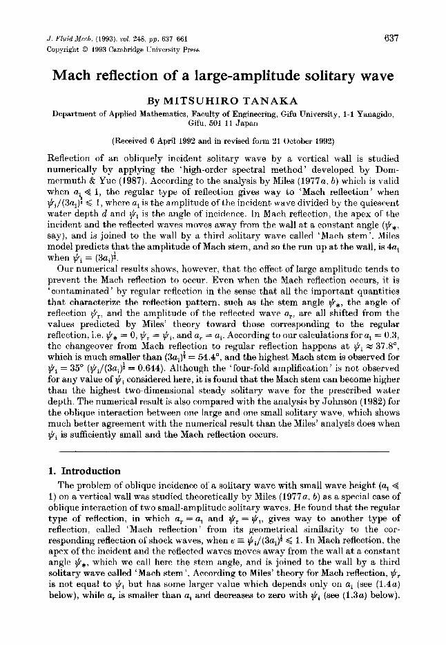
FIGURE 1. Schematic representation of Mach reflection pattern.

increasing even at the end of the measurement, suggesting that his experimental apparatus does not have enough length to observe such a slow process as Mach reflection.

Because the comparison of the numerical results with the theoretical prediction by Miles is the central subject of this work, it is worthwhile summarizing here the main results obtained by Miles, which are valid when a, < 1.

(i) The regular type of reflection gives way to Mach reflection when E = $,/(3ai); becomes less than 1.

(ii) step angle $* (see figure 1) :

l-e) Mach reflection, ( l . l a )

regular reflection. ( 1 . l b )

(iii) amplitude of Mach stem aM (or the maximum run-up a t the wall)

(1 +# Mach reflection, (1.2u)

4/11 + (1 - 1/c2);] regular grazing reflection, (1.2b)

2 + [ 3 / ( 2 sin2 llri) - 3 + 2 sin2 $,] ai regular non-grazing reflection. ( 1 . 2 ~ )

(iv) amplitude of the reflected wave a,.:

a, -/ e2 Mach reflection, - -

ui I 1 regular reflection.

( 1 . 3 ~ )

(1.3b)

640 M . Tanaka

(v) angle of reflection ~ r :

~~ = { (3ai)g Machreflection,

+i regular reflection.

( 1 . 4 ~ )

(1.4b)

In the next section, we explain the method of numerical calculation. As an overall test of the scheme, we also show the result of a two-dimensional calculation for the head-on collision of two identical solitary waves, which is equivalent to the normal incidence of a solitary wave on a rigid vertical wall. The numerical result for oblique incidence is shown and compared with Miles’ theory in $3. It is also compared with the analytical result by Johnson (1982) for oblique interaction between one large and one small solitary wave. Conclusions are given in $4.

2. Numerical method 2.1. Dommermuth & Yue’s scheme

We consider the irrotational motion of inviscid and incompressible water under a free surface with a constant finite depth. For simplicity, we normalize the space and the time in such a way that both the gravitational acceleration g and the quiescent water depth d are unity. Then the velocity field can be described by a velocity potential $(x, y, z , t ) which satisfies Laplace’s equation throughout the water region. where x and y are horizontal coordinates and z is the vertical coordinate pointing upward.

In terms of the velocity potential at the free surface @(x, y, t ) = #(x, y. ~ ( x , y, t ) , t ) , with ~ ( x , y, t ) being the displacement of the free surface, the kinematic and dynamic boundary condition on the free surface are respectively

yt = -V, #s’vh 7 + W[l+ (vh 7)2], (2.1)

$f =-?1- t [v ,~S]z+~W2[1+(Vhr)2 ] , (2.2)

where Vh 3 (a/ax, a/ay), and W(x , y, t ) is the vertical component of the velocity at the free surface. The boundary condition at the bottom is

# , = O ( z = - 1 ) . (2.3)

We assume that $ can be approximated by a perturbation series in a small parameter which is a measure of wave steepness, and write

where M is the order of approximation. By expanding each $(m) in a Taylor series about z = 0, we have

Expanding (2.5) and collecting terms of each order, we find

$“’ (X ,Y,O>t ) = $S(.,Y,t),

(2.6) $(m)(x, y , O , t ) = - m-l 2 - 7 $ m - k ) ( X , y , O , V k ak t ) (m = 2 ,3 , ...) M ) . Ic=l k ! az

These boundary conditions and Laplace’s equation gives a series of well-defined boundary-value problems for $(m) , which can be solved successively once #’ and y are

Mach reJlection of a large-amplitude solitary wave 64 1

prescribed. The crucial point in this procedure is that the original Dirichlet problem for $(x, y , x , t ) with a complex boundary given by z = ~ ( x , y, t ) has been transformed to a series of Dirichlet problems for qVm)(x, y, z , t ) (m = 1,2 , . . ., M ) with a very simple boundary z = 0.

When the wave field is periodic in horizontal coordinates with L, and L, as the period in each direction, qVm) can be expressed by a double Fourier series as

with Kk, 1 E [(27ck/L,)2 + (27cf?/L,)2]t.

The coefficients cimi can be obtained by one two-dimensional fast Fourier transform (FFT) when qVm)(x, y,O,t) is given by (2.6), and qVm) is thus obtained quite easily. Once #m) (m = 1,2, . . . , M ) are all known, the vertical velocity at the free surface W can be obtained by

and then the values of qF and 7 can be updated by the boundary conditions (2.1) and (2.2).

Although 7, $ ( m ) , and W are all represented by their Fourier coefficients, the products between them are performed in the physical space instead of the spectral space. In this respect, the scheme is pseudospectral, and it suffers from the aliasing error. We removed this aliasing error by applying the standard ‘$rule’ (see for example Canuto et al. 1988) every time two functions are multiplied.

It is not a new idea, even within the context of strongly nonlinear water waves, to assume periodicity in each direction and express the physical quantities by their Fourier series in order to facilitate numerical calculations. For example, Fenton & Rienecker (1982) also used Fourier methods in their numerical study of two- dimensional interaction between large-amplitude solitary waves. However, as Dommermuth & Yue (1987) discuss Fenton & Rienecker’s scheme satisfies the free- surface boundary conditions by collocation on the exact free surface, and the operation count per timestep increases typically as N3 with N being the total number of mesh points. In Dommermuth & Yue’s scheme, on the other hand, the free-surface boundary conditions are transformed to M boundary conditions on the undisturbed flat surface, each of which can be solved quite easily by the use of FFT, and the operation count increases only as N In N in N , and roughly as M2 in M . This great reduction in the operation count has enabled us to perform the three-dimensional calculations reported here with a reasonably large number of mesh points in both directions. (Dommermuth & Yue claim that the operation count of their scheme increases only linearly both in N andM when FFT is used. However, we believe that, as the double sum in (2.5) and (2.8) suggests, the number of products, and so the number of FFTs which need to be called to remove the aliasing error, should increase almost quadratically in M instead of linearly.)

2.2. Initial condition The region considered in the numerical calculation is 0 < x < L, and 0 d y < L, (see figure 1) . The impermeable condition at the rigid wall (x = 0) is automatically satisfied by assuming that ~ ( x , y, t ) and @(x, y, t ) are both even functions with respect

642 M . Tanaka

to x. Then 7 and 4' are even periodic functions of x with half-period L,, and are expressed by cosine series. With regards to the y-coordinate, we also assume periodicity with period L, which is taken sufficiently long, and use an ordinary Fourier series with sines and cosines in representing q and #'. We employ the third- order steady solitary wave solution obtained by Grimshaw (1971) for the initial condition. The wave profile 7 and the propagation speed (or Froude number) F are expressed as follows when it propagates in the positive x-direction

,$? = a s 2 _ ~ 2 ( s 2 - S 4 ) + a 3 ( ~ s 2 - ~ S 4 + 1 0 1 8 0 ' 6 )+0(a4), (2.9)

where s E sech{a(x-Pt-x,)}, ( 2 . 1 0 ~ )

F = 1++a-&u2+&a3+O(a4), (2.10b)

a = (@)"l-~a+&a2)+O(a~) =D-1. (2.104

In our calculations of oblique incidence, the initial solitary wave has a crest line which is parallel to the line y = -tan $, x x, and is propagating in the direction ( -sin lCri, - cos $i) (see figure 1 ) . When we compare the third-order steady solution with the ' almost exact ' solution obtained numerically by the method described in Tanaka (1986) for a = 0.3, which is the largest value of ai we consider here, we find that these are almost identical in every respect. For example, the Froude number F, the excess mass, and the potential energy of the 'exact' solution are 1.13752, 1.36197 and 0.13360, respectively, and the relative errors to these quantities involved in the third-order solution are 3.7 x and 5.3 x lop3, respectively. We think this fact justifies our use of the third-order solution as the initial condition, provided a, d 0.3.

The intervals of numerical mesh points Ax and Ay are determined as follows. When the wave height ai of the incident solitary wave and the angle of incidence $i is prescribed, we require first that

6.4 x

Ay = Ax tan $i. (2.11)

This implies that any straight line connecting mesh points ( i , j ) and (i + 1, j- 1 ) (or the line i +j = constant) is parallel to the crest line of the incident wave, and that Ax automatically becomes much larger than Ay when lCri becomes small and the typical lengthscale of variation in the x-direction (i.e. the direction normal to the wall) becomes much longer than that in the y-direction (i.e. the direction parallel to the wall). Next we require that the distance between the two adjacent straight lines, i+j = m and i+ j = m+ 1 (m = some arbitrary integer), both parallel to the crest line of the incident wave, is of the typical lengthscale of the incident solitary wave D given by (2 .10~) . These two requirements determine Ax and Ay as

AX=- (2.12)

The dimensions L, and L, of the numerical region are determined from these mesh interval and the number of mesh points by L, = N, x Ax and L, = N , x Ay, respectively. In most of the calculations shown below we take N, = 128 and N, = 512.

Mach reJlection of a large-amplitude solitary wave 643

2.3. Condition at the oflshore boundary x = L, The condition at the offshore boundary x = L, needs some care. As explained previously, we assume that q(x,y,t) and qP(x,y,t) are both even and periodic functions of x with half-period L, in order to use Dommermuth-Yue's methodology taking into account the impermeable boundary condition at the wall (x = 0). However, when we extend the initial condition as described above periodically beyond 0 < x < L,, we realize that the crest line of the initial solitary wave is a 'zig- zag' and has an angular corner with inner angle ?t - 2$i a t x = L, (or odd multiples of L,) which is pointing toward the direction of propagation (i.e. negative y- direction). However, such an angular corner in the crest line would diffuse out as time elapses, as discussed below, implying that we need some artifice in the treatment of the region near x = L, in order to keep such an angular corner for t > 0.

Let some part of the straight crest line of a solitary wave be pushed forward and become convex toward the direction of propagation. Then each line element of this bent crest line would propagate in a diverging direction, and consequently the part of the crest line would be stretched. Then the law of energy conservation requires that the wave height of this part should be decreased in order to compensate for the stretch of the crest line. On the other hand, the propagation speed of a solitary wave decreases with its wave height except for the vicinity of the limiting solitary wave with wave height 0.827. This implies that the part of the crest line which is convex toward the direction of propagation would propagate more slowly, and consequently the crest line tends to recover the original straight line. Exactly the opposite thing would happen when a part is pushed backward to become concave toward the direction of propagation. In this sense, the solitary wave is stable to a bending disturbance. The linear stability analysis of the solitary wave solution of the Korteweg-de Vries ( K 4 V ) equation to a bending disturbance with very long wavelength was studied analytically by Kadomtsev & Petviashivilli (1970) based on the two-dimensional K-dV equation, which is also called the K-P equation named after them. Tanaka (1990) also studied this process of the returning of a bent solitary wave to a solitary wave with a straight crest line by integrating numerically the second-order mode-coupling equation by a fast pseudospectral scheme he developed.

We plot in figure 2 a perspective view of the free surface at t = 30 when a, = 0.3, $i = 40" in order to see what happens to the crest line of the incident solitary wave around x = L,. It can be seen clearly that the angular corner which existed initially a t x = L, has diffused out, and the crest line has become a smooth curve with finite curvature. The decrease of wave height around x = L, is also appreciable. The region with curved crest line and decreased wave height spreads to a wider region as time elapses. Because the problem we are trying to simulate is the interaction with the wall of a solitary wave which has a straight crest line of infinite length and uniform wave height along it, we need some artifice which prevents this diffusion of curvature and depression of wave height from affecting the wave motion in the interaction region near the wall. If we try to overcome this numerical difficulty naively by taking L, (and so L, because the crest line of the incident wave is inclined) very long, the total number of points N ( = N, xN,) would become so large that the numerical calculations would require prohibitively long CPU time.

The first method we tried was to replace, at some fixed interval of time, qi+l,j-l (= q ( ( i + l ) A x , ( j - 1 ) A y ) ) and @+l,,-l with q6,r and @, for i, < i GiV,, 1 < j <Nu, with i, being some suitably chosen number (80% of N,, say). Remember that any straight line connecting two mesh points (i,j) and (i + 1,j - 1) is parallel to the crest

644 M . Tanaka

1 .o

0.8

v) 0.6 2c

0.4

.-

0.2

0

0

400

FIGURE 2. The free-surface displacement without the artificial modification of data around x = L,. ai = 0.3, +i = 40, t = 30.

line of the incident solitary wave. This seems to be the simplest method by which we can recover a straight crest line with prescribed angle of incidence and a constant wave height along it near x = L,. This method is also convenient for our scheme in the sense that it does not disturb the periodicity in the y-coordinate. It turns out, however, that as this method modifies the data for the whole range of y, it is apt to affect the reflected wave as well as the incident wave when the reflected wave grows and elongates with time. Because this artificial modification of data is suitable exclusively for the incident wave, the computation explodes, as expected, soon after the tip of the reflected wave comes close to the line x = i, x Ax.

In the second method, and this is the method that we employ in all the calculations reported here, the artificial modification of data

(2.13)

is restricted to a much narrower region than in the first method. First we move along the line i + j = const., which corresponds to the crest line of the incident wave, and if the deviation of q from a, becomes larger than 0.5% of ai, we draw through this point a straight line normal to the crest line of the incident wave. Then the modification of data (2.13) is performed only in the trapezoid enclosed by this line, the numerical boundary x = L, and the two lines both parallel to the crest line of the incident wave, one in the front and another in the rear of the incident wave. The distance between these two parallel lines is tentatively chosen to be 15 times (10 for the rear and 5 for the front side of the incident wave) the distance which the incident solitary wave has propagated since the straight crest line and constant wave height were recovered by this method last time. We applied this artifice with a fixed time interval of 1 .

Once we introduce this artificial modification of data, the system is no longer

Mach reJlection of a larye-amplitude solitary waue 645

closed, and does not have any conserved quantity which would be useful in checking the accuracy of calculation. Then, in order to know the suitable values of At a,nd M for each case, we first run a preliminary calculation without applying the modification of data as above whenever ai and/or $i is changed, and monitor the constancy of mass, momentum and energy. For example, when we use At = & and M = 3 for the case of a, = 0.3, $i = 40", the total energy E which is defined in the fully nonlinear manner as

(2.14)

remains constant with relative error less than 0.2 % until t = 120, by which time the incident solitary wave has propagated more than 136 times the water depth. From this result of the preliminary run, we can expect that these values of At andM, as well as Ax and Ay chosen by the principle explained in the previous section, would give reasonably accurate result for this combination of ai and $i when the artificial modification of data as described above is introduced and the system becomes no longer closed. Integration with respect to t is performed by the fourth-order RungeKutta-Gill method.

We have employed M = 3 for all the cases reported here, and for two specially chosen cases with a, = 0.3, $i = 35", and ai = 0.3, = 20", we have also calculated with M = 4. The first case we think is important because it gives the highest run-up at the wall in all the cases considered, while the second case shows quite clearly the occurrence of typical Mach reflection. We do not think that these relatively small values ofM are large enough to obtain very accurate results, and we cannot deny that the limitations of the budget and the storage of the computer (FACOM VP2600 of Nagoya University) were among the important factors in choosing the values of M (and alsoN). However, the difference in the maximum run-up a t t = 150 between the calculations with M = 3 and M = 4 is only 2 % when ai = 0.3, @i = 20°, and it still remains about 4% even for the case a, = 0.3, $i = 35" in which the maximum run- up at the wall exceeds 90% of the quiescent water depth. From these facts, we believe that our results are reasonably trustworthy, not only qualitatively but also quantitatively.

Moreover, it should be noted that the calculation with M = 3 (or 4) must give a more accurate result than the third- (or fourth-)order approximate equation for weakly nonlinear long waves. For weakly nonlinear long waves, we have two small parameters a ld and d/h with a being the typical wave height, d the water depth, and h the typical horizontal lengthscale, and in the theoretical treatment it is usually assumed that

(2.15)

With this scaling, the steepness ak of the wave, which is the only parameter that we assume small in the present scheme, is O($). When we count the order of approximation of the calculation by M , we are talking about theMth power of a k and not that of 6 as in the perturbation theory for weakly nonlinear long waves.

2.4. Test calculation for normal incidence (two-dimensional problem) Before proceeding to the three-dimensional calculation of oblique incidence, we performed one calculation for the head-on collision of two identical solitary waves, which is equivalent to the problem of reflection of a normally incident solitary wave

646 M . Tanaka

t = 16

il t = O I1

V. 1

- 80 - 60 - 40 - 20 0 X

FIGURE 3. The free-surface displacement versus x and t of a solitary wave of a = 0.3 reflecting from a wall. t = 0, 2, 4, ..., 70.

by a rigid vertical wall, as an overall check of our numerical scheme except for the artificial modification of data described above. This problem has already been investigated by various authors (see, for example, Byatt-Smith (1988) and the references therein).

The initial condition of our calculation consists of two third-order solitary waves (equations (2.9) and (2.10)) with ai = 0.3 which are separated 1 4 0 (!z 34.2) apart withB given by ( 2 . 1 0 ~ ) . With this condition, the surface displacement at the middle point of the two solitary waves is less than 1.7 x iO-6. As the Froude number F given by (2.10b) is about 1.14 when ai = 0.3, the solitary waves would collide around t = 15. Various parameters of the numerical calculation are chosen as follows: N, = 256, Ax = $D, L, = N, x Ax = 64D, At = i, and M = 3. By the end of the calculation t = 70, the total energy E defined by (2.14) has changed only less than 0.13 % of its initial value, and the total CPU time is about 1.5 s on FACOM VP2600 of Nagoya University.

Figure 3 shows the surface profile a t various timesteps at a constant interval for 0 < t d 70. Although ai is not the same, the present result looks very similar to that obtained by Mirie & Su (1982) (see their figure 2). Our result reproduces the significant secondary wavetrains trailing each of the solitary waves which was predicted theoretically by the third-order perturbation analysis of Su & Mirie (1980). It is also observed clearly that both the wavelength and the amplitude of each of the secondary wavetrains decrease as the distance from the solitary wave increases in accordance with Su & Mirie’s prediction.

Fenton & Rienecker (1982) also investigated the same problem by solving numerically the full system of equations for surface gravity waves by their Fourier method, but did not succeed in reproducing such secondary wavetrains. Byatt-Smith (1988) argues this drawback of Fenton & Rienecker’s calculation as if it were intrinsic to all the ‘Fourier methods’ which impose some artificial periodicity on the wave field and represent 7 and q5 by their truncated Fourier series. However, our numerical result shown above indicates that this is not the case and that the ‘Fourier methods’

Mach rejlectiorz oj a larye-amplitude solitary wave 647

are capable of describing the dispersive tail as well as the main part of the wave correctly if they are used properly. We suppose that the drawback of Fenton & Rienecker’s calculation has stemmed from just the insufficiency of the length of spatial period they imposed on their calculation.

We observe from our numerical result that the maximum value Aa of the transient loss of amplitude of the solitary wave which occurs immediately after the reflection is about 0.0150. The perturbation analysis by Byatt-Smith (1988) shows that this quantity is O(a:) and is given by 0.4938 x a:, giving 0.0133 for the present value of a,( = 0.3). Bearing in mind the rather coarse discretization in both x and t as well as the relatively lower order of nonlinearity (M = 3) and large value of maximum runup ( - 0.649), the agreement between theory and numerical result seems to be quite satisfactory. The calculation with M = 4 gives Aa = 0.0132, and the agreement with Byatt-Smith’s prediction is still better. The numerical result seems to have converged by this value of M , and any further increase of M makes no difference in Aa. We believe that our numerical scheme is also able to detect the final loss of amplitude, which Byatt-Smith’s analysis predicts to be O(a!), if the value of M is suitably chosen. However, this problem is not relevant to the main subject of this work, and we will not pursue i t any further here.

3. Results for oblique incidence 3.1. atdependence (9i/(3ai)i - 0.74)

In order to see how the effect of large amplitude modifies the predictions given by Miles for waves with small amplitude, we first study three cases with different amplitude a, of the incident wave. The angle of incidence $i is also changed correspondingly in such a way that B = 9,/(3a,)1 remains almost constant. In this sense, these three cases would have almost the same likelihood of producing Mach reflection. The cases we have chosen are a, = 0.1, @i = 23” ( E = 0.733), a, = 0.2, $i = 33” (6 = 0.744) and a, = 0.3, 9, = 40” ( B = 0.736).

It should be stressed again here that Miles’ theory is valid only for a, < 1 , while almost all of the cases treated here are in the regime where Miles’ theory cannot be expected to hold. In the following argument we often use a phrase like ‘the value predicted by Miles’ theory’, but this should be understood as a value which we obtain if we apply one of the expressions (1.1)-(1.4) naively to those cases for which the condition ai Q 1 is not satisfied. Thus the disparity between the numerical result and Miles’ theory is just to be expected.

As the free-surface displacement of the typical Mach reflection pattern shown in figure 4 indicates, the incident and the reflected waves obtained numerically have some finite width with some inner structures in it, and they cannot be expressed simply by two straight lines, as that schematically shown in figure 1. This brings out some ambiguity in determining the position of the apex of the incident and the reflected waves, and so the length of Mach stem 1,. In this paper, we define I , by the distance measured along a straight line normal to the wall which joins the point of maximum run-up a t the time and the point off the wall where the free-surface displacement decreases to a,. Once 1 , and the point of maximum run-up are known for various timesteps, the stem angle +* can be obtained easily.

We show the results for a, = 0.1 and ai = 0.3 in figure 5 and figure 6, respectively. Figures 5 (a) and 6 (a) show the evolution of aM as a function of time t , while figures 5 ( b ) and 6 ( b ) show that of 1,. The dashed line in each of the figures denotes the prediction given by Miles’ theory.

648 M . Tanaka

1.0

0.8

0.6 x z 0.4

._

0.2

0

FIGURE 4. Typical free-surface profile around the Mach stem. ai = 0.3, $i = 20°, and t = 170.

3

QM - 2 a,

I

20

10

0 F 100 200 300 0 100 200 300 t t

FIGURE 5. (a) %/a, us. t. a, = 0.1, = 23'. ( b ) 1, us. t. a, = 0.1, +i = 23'.

When ai = 0.1, y+i = 23", the maximum run-up, which is still increasing slightly at t = 300 and has not saturated yet, appears to asymptote to some value close to 3.00 in accordance with Miles' prediction. The length of the Mach stem 1, is also increasing almost linearly in t , although the rate is noticeably smaller than predicted. From these results, we can infer that a Mach reflection as described by Miles is actually occurring for this case except for quantitative agreement.

When a, = 0.3, $i = 40°, on the other hand, the maximum run-up has almost saturated by the time t w 100 at a value slightly larger than 2 . 4 ~ ~ ) which is only 80% of the value predicted by (1.2a). The length of the Mach stem also seems to have stopped growing, and the elongation of the Mach stem linear in t , which is an important indication of Mach reflection, is hardly observed. Figure 7 shows the wave

Mach reflection of a large-amplitude solitary wave 649

0 50 100 t

FIGURE 6. (a) aM/ai 'us. t . a, = 0.3,

10

0 50 100 t

40". ( b ) 1, V 8 . t . Ui = 0.3, $, = 40'

3

2

- 11 ai

1

0 50 100 X

FIGURE 7. Wave height along the crest line of the reflected wave. t = 10, 20, 30, ..., 120.

ai = 0.3, $, = 40".

height along the crest line of the reflected wave (and the Mach stem) at various time steps. If the Mach reflection as predicted by Miles' theory occurs, the amplitude a, of the reflected wave should be 0.542ai which is shown in the figure by the dashed line. The figure shows, however, that a, is more than 95 % of a, at t = 120, and it looks like growing towards the asymptotic situation with a, = a,. This indicates that the reflection which is occurring for this case is a regular reflection rather than a Mach reflection even though E = 0.736 and is less than 1.

From these results, it may be inferred that the effect of large amplitude tends to prevent the Mach reflection occurring even when $J(3ai); < 1.

3.2. $i/(3a,)i-dependence (ai = 0.3) Next we investigate how the reflection pattern which actually happens differs from that predicted by Miles' theory both qualitatively and quantitatively for various values of +i in the range 10' < +i < 60°, with a, being fixed at 0.3.

650

(a) 300

I , I I I l l I , I (c)

50 -

40 -

,' I , 30 -

M . Tanaka - 4 7 - - 1

-

-

-

(4 3

2

7 - a,

As a typical example of the cases in which Mach reflection occurs, we show in figure 8 the result of the case $i = 20" (6 = 0.368). I n each of the figures except for figure 8 (a ) , the theoretical prediction by Miles is shown by a dashed line. Figure 8 (a ) shows the patterns of crest lines of the incident and the reflected waves for 0 < t 6 150 with a constant interval of time. It can be seen clearly that the apex of t,he incident and the reflected waves is moving away from the wall a t a constant angle. It can also be observed that the angle of reflection $r is about 42.8" ((1.4a) gives = 54.4"), and is appreciably larger than $i. The right end of the figure corresponds to the numerical offshore boundary x = L,, and the artificial modification of data explained in $2.3 seems to be working satisfactorily. The evolution of aM and 1, are shown in figures 8 ( b ) and 8 ( c ) , respectively. The Mach stem has a larger amplitude than expected from ( 1 . 2 ~ ) . Figure 8 ( c ) clearly shows the elongation of the Mach stern which is linear in t . However, the stem angle $* calculated from this is 6.92" and is significantly smaller than the 11.45" predicted by ( 1 . 1 ~ ~ ) . The wave height along the crest line of the reflected wave (and Mach stem) is plotted in figure 8 (d ) at a constant interval of time for 0 < t d 150. It can be observed that the reflected wave remains much smaller than the incident wave in accordance with Miles' theory. However, a, obtained numerically is about 0 . 2 3 ~ ~ and is significantly larger than the 0 . 1 3 5 ~ ~

Much reflection of a large-amplitude solitary wave 65 1

1 11

0 20 40 60 80 t

0 20 40 60 80 x

FIGURE 9. (a) Pattern of crest lines of the incident wave, reflected wave and the Mach stem. a, = 0.3, @i = 60". t = 0, 10, 20, ..., 90. (b) u,/u, US. t . a, = 0.3, y?i = 60". (c) 1, US. t . U, = 0.3, @, = 60". (d) Wave height along the crest line of the reflected wave. a, = 0.3, y?i = 60". t = LO, 20,30, ..., 90.

which (1.3a) predicts. From these facts, we can infer that the reflection we observe for this case is nothing but a Mach reflection as far as its geometry is concerned. But when we compare it quantitatively with the theoretical prediction by Miles, we realize that the reflection pattern which we observe numerically is consistently shifted toward the regular reflection in the sense that $r is smaller (i.e. closer to $J> a, is larger (i.e. closer to ui), and $* is smaller than expected from (1.4a), (1.3a) and ( 1.1 a ) , respectively.

The above results are obtained by a calculation with M = 3. In order to see if this value of M is reasonable for the present case with a, = 0.3, = Z O O , we performed another calculation with M = 4, and found that the difference between the two calculations is satisfactorily small. For example, the calculation with M = 3 gives aM = 0.6125 and I, = 26.03 at t = 150, while the one with M = 4 gives aM = 0.6252 and 1, = 25.89 a t that time, and the relative errors in these quantities are 2.0% and 0.5%, respectively. From this comparison, we can be confident that M = 3 is reasonable for the present, case and that the results obtained are trustworthy.

The results for the case $i = 60' ( E = 1.104) are shown in figure 9 as a typical example of the cases with regular reflection. Each of the figures corresponds to its counterpart of figure 8. It can be seen in figure 9 ( a ) that the apex of the incident and the reflected waves always remains close to the wall, and that $, is equal to $i.

652 M . Tanaka

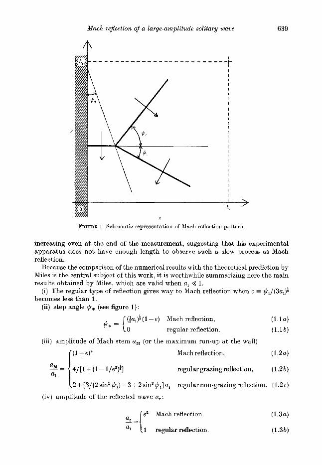
FIGURE 10. .,/ai 08. @i. (a, = 0.3).

Figure 9 ( b ) shows that the maximum run-up has reached its asymptotic value aM - 2.1 lai by t - 15. The two dashed lines in the figure correspond to the two expressions given by Miles, one for regular grazing reflection (1.2 b) and the other for regular non- grazing reflection (1 .2~ ) . It can be seen that the expression for regular non-grazing reflection gives a very good approximation even for a, = 0.3. In figure 9 ( d ) we plot the wave height along the crest line of the reflected wave, which shows the growth of the reflected wave towards the final situation with a, = a,.

3.2.1. aM iis. $i We show in figure 10 the maximum run-up aM a t the wall as a function of $, for

ai = 0.3. In this figure, as well as in figures 11-14, the dashed line corresponds to the result obtained by Miles for a, < 1.

It is generally true that the regular reflection reaches its asymptotic state much faster than the Mach reflection does. (Compare, for example, figures 8 ( b ) and 9 (b ) and see the big difference in the timescale of the evolution.) Expression (1 .1 a) for $* also shows that the rate of elongation of the Mach stem is proportional to (1 - 6 ) as well as (a,):, As the Mach stem should become infinitely long for the asymptotic state to be achieved, this dependence of +* on e suggests that, when a, is constant, the speed of convergence towards the asymptotic state would become slower and slower as $i

approaches from below the critical value corresponding to the changeover from Mach reflection to regular reflection, which we will show later to occur a t $i - 37.8' when a, = 0.3. I n all the cases except the one with I), = 35", the temporal variation of aM becomes sufficiently small towards the end of the calculation, and we believe that the value of uM at the end of the calculation is reasonably close to the value which aM would take when t + 03. For the case with yki = 35", on trhe other hand, the convergence to the asymphotic state is very slow as the above argument suggests, and aM is still increasing gradually a t the end of the calculation t = 150. The bracket in figure 10 is to express this insufficiency of convergence. The true asymptotic value of aM for this case may be somewhat larger than that shown in the figure.

Mach rejection of a large-amplitude solitary wave 653

It can be seen in figure 10 that the agreement between the numerical result and Miles' prediction is quite satisfactory while $i is small. As y+, becomes larger, the deviation between the two increases gradually up to +i - 30". Then at somewhere between $, = 35" and 40", the numerical result suddenly starts to decrease and remains almost constant a t around 2. lai afterwards. The sudden change strongly indicates that the changeover from Mach reflection to regular reflection has occurred there, where $i is much smaller than (3a$ = 54.4".

There is no region of $, where the expression for regular grazing reflection (1.2b) is useful for this value of a,. On the other hand, the coincidence between the numerical result and the theoretical prediction for regular non-grazing reflection ( 1 . 2 ~ ) is impressive when +i 2 40". Funakoshi (1980) also reports that the numerical result agrees very well with the prediction for non-grazing reflection rather than that for grazing reflection when +,/(3ai)+ > 1.3 , i.e. @, > 29" for the value of a, ( = 0.05) he studied. It seems that ( 1 . 2 ~ ) is quite robust, and remains a good approximation even when a, becomes large, provided $, is also large enough. We know from experience that the K-dV equation, which is just the lowest-order approximation with respect to the non-linearity and dispersion, is quite robust and gives satisfactory approximation of actual wave motion even when the amplitude of the wave is by no means small. We suppose that the robustness of ( 1 . 2 ~ ) which we observe in figure 10 has stemmed from the same origin as that of the K 4 V equation.

This remarkable usefulness of ( 1 . 2 ~ ) for larger values of $i also restricts severely the amplification of the Mach stem. When a, = 0.3, the theoretical curve for Mach reflection (1 .2a) enters the region of $i where ( 1 . 2 ~ ) appears to be valid well before it attains its maximum value of 4 a t $, = (3a,)t = 54.40. Let us suppose tentatively that the expression (1.2 c) for non-grazing reflection holds when y+, 2 35" irrespective of a,. Then it may be conjectured that the 'four-fold amplification' would occur only for those values of a, which satisfy (3ai)i < 35O, i.e. a, < 0.12. In any event, the 'four- fold amplification', which would be quite dangerous for coastal structures if it ever happens, does not seem to occur for any value of @i unless a, is sufficiently small.

It should be noted, however, that, according to the result shown in figure 10, the maximum run-up aM is 0.869 a t t = 150 when aI = 0.3, @, = 35. This implies that the amplitude of the highest two-dimensional steady solitary wave (= 0.827) does not give the upper bound for the maximum run-up at the wall. Like most of the other calculations reported here, the above result is obtained withM = 3, but there is some doubt whether M = 3 would be sufficient for a large wave which is even higher than the highest steady solitary wave. Then, as we did in the case of a, = 0.3, $, = 20°, we carried out another calculation with M = 4, keeping Ax, Ay and At the same, and obtained aM = 0.905 a t t = 150, which confirms that the Mach stem can become higher than the highest two-dimensional steady solitary wave. It should be noted, however, that we are not talking about the asymptotic value of aM as t --f 00. We are just claiming here that the Mach stem can become higher than the highest steady solitary wave in the evolution process of Mach reflection. We will return to this point again a t the end of this section.

The maximum run-up which the calculation with M = 4 gives is about 4 YO larger than that given by the calculation with M = 3, and this difference can be regarded as a rough measure of the magnitude of truncation error involved in the calculation. As it is quite likely that the truncation error is largest for the case in which the largest wave appears, the magnitude of the error that we have just seen for the case with a, = 0.3, $, = 35" would probably give the overall upper bound of truncation error for all the calculations studied here.

654 M . Tanaka

FIQURE 11. $r 'us. +,. (a, = 0.3).

3.2.2. $,, a, and $* us. $i

The angle of reflection $, is plotted in figure 11 as a function of $i. It shows that $r does not remain constant at 54.4" in the region of Mach reflection as Miles' model predicts, but it decreases gradually as +i increases. Consequently, it meets the line 4, which corresponds to the regular reflection, at a smaller value of $i than (3ai)r, making the changeover from Mach reflection to regular reflection happen earlier than expected from Miles' theory for ai 4 1. It will be shown below that this behaviour of can be explained to some extent by Johnson's analysis (1982) on oblique interaction between one large and one small solitary waves.

Figure 12 shows a, as a function of +i. By a,, we mean the largest displacement of the free surface along the crest line of the reflected wave (see, for example, figure 8d) . It can be seen that the reflected wave consistently has a larger amplitude (i.e. closer to ai) than that predicted by (1.3a) except for the one case with +i = 60' ( E = 1.104), for which Miles theory also predicts the appearance of regular reflection and hence gives ur/ai = 1.

The stem angle +* is plotted in figure 13 as a function of $i. The figure shows clearly that the elongation of the Mach stem is consistently slower than predicted by (1.la). It also shows that $* decreases almost linearly in $i and vanishes at $, x 37.8", implying that the changeover from Mach reflection to regular reflection happens there. Although, unfortunately, the original reference is not available to us, Wiegel(l964) quoted that Chen (1961) performed wave-tank experiments for various values of a, and observed the critical angle to be between 35" and 40". This seems to be consistent with the critical angle which we have obtained (= 37.8") for ai = 0.3. The critical angle is also the most dangerous angle of incidence from the view point of coastal protection because it brings about the highest run-up at the wall for an incident solitary wave with prescribed wave height, and it seems to be of great importance to know the critical angle of incidence as a function of a,. We will pursue this problem in the near future.

Mach rejlection of a large-amplitude solitary wave

I .6

1.4

1.2

1 .o a, - 0.8 ai

0.6

0.4

0.2

0 20 40 60

11.l (deg) FIGURE 12. uJa, vs. @,. (a, = 0.3).

20

655

0 20 40 60

11.i (deg) FIGURE 13. $* vs. gi. (u, = 0.3).

3.2.3. Cornparison with Johnson (1982) Johnson (1982) extended Miles’ analysis of oblique interaction between two small

solitary waves to the one between a large solitary wave and a small one. Unfortunately, he did not apply the result of his analysis to the reflection problem which we are now concerned with, and did not give any explicit expressions for a M , $r or a, as functions of a, and $i which would correspond to the expressions (1.1)-(1.4). However, he obtained the condition for resonant interaction (i.e. l,ul = v by his notation) which gives one relation between the amplitudes of large and small

656 M . Tanaka

80

s

FIGURE 14. @r given 0, by the present calculation and +, those given by Johnson’s analysis vs. $i. a, = 0.3. ---, prediction by Miles’ theory.

waves and the angle between them, and we can examine to what extent this condition is satisfied by the reflection pattern which we have obtained numerically. In the reflection problem, the large and the small solitary waves in Johnson’s analysis correspond, respectively, to the incident and the reflected waves, and the angle 8, - 8, between the two solitary waves in Johnson’s analysis corresponds to $i + $, in the reflection problem. The Froude number F of the steady solitary wave with a, = 0.3 is 1.1375, and (520) (i.e. equation (20) of Johnson’s paper) determines a as 0.8071 for this value of F . (It should be noted that FI on the left-hand side of (520) should read F:.) Then (525) gives A, = 0.6722, with A, = COS($~+$,),. This implies that the weak interaction approximation breaks down when $i + $, = 47.76” if a, = 0.3. This corresponds to the breakdown of the weak interaction that Miles encountered for two small-amplitude waves propagating nearly in the same direction. The resonance condition I,ul = v, together with (J48a)’ determines A as 1.0166, and finally we obtain the following relation between a,, $i and $,,

$, = c0s-l(Ac - at A ) - $i. (3.1)

In figure 14, we show $, given by (3.1) by solid symbols as a function of $i when the values for a, are obtained numerically and shown in figure 12. For the sake of comparison, we also plotted the values of $, obtained numerically by open symbols and those given by (1.4) by the dashed line. It can be seen that Johnson’s theory agrees much better with the numerical result than Miles’ theory does for all the values of ki that correspond to Mach reflection, i.e. $i < 37.8’. The agreement between the two is quite satisfactory especially for smaller values of for which a, is also small (see figure 12) and hence the assumption underlying Johnson’s analysis that one of the two interacting waves is very small is valid there. Unlike Miles’ theory which predicts that $, will remain constant when $i < (3a,)4, Johnson’s theory can explain satisfactorily the numerical observation that $r decreases gradually as $i

increases and so does a,. It can also be observed in figure 14 that $r obtained

Mach re$ection of a large-amplitude solitary wave 657

0.7

0.5

'1 0.3

0.1

0 I00 200 300

Y FIQURE 15. The free-surface displacement along the wall vs. y and t . ai = 03, ll.i = 20,

t = 0 , 10, 20, ..., 170.

numerically (open symbol) seems to asymptote correctly to $,. = 47.76' as $1+0, i.e. to the value of $, which Johnson's theory (3.1) gives when ai + O . This fact certainly indicates that our numerical result is reasonably accurate at least for smaller values

Among all the oblique incidences of a solitary wave with prescribed wave height, those with $i equal to or slightly less than the critical angle of incidence are certainly of greatest practical importance because they bring about the highest run-up a t the wall. The reflected wave for these cases has nearly the same wave height as that of the incident wave as shown in figure 12, and Johnson's analysis cannot be expected to hold for them. However, the result shown in figure 14 indicates that Johnson's prediction, although it deteriorates as expected as ll.i approaches the critical angle of incidence $i = 37.8" and hence ar becomes larger, shows satisfactory agreement with our numerical result throughout the range of $i which corresponds to the Mach reflection. From this fact, we think it would be worth pursuing the reflection problem further along the line of Johnson's analysis and deriving explicit expressions for a,, aM, 9, as functions of a, and $-i as those derived by Miles and shown in (1.1)-(1.4).

3.2.4. Much stem as t + co We show in figure 15 the surface displacement along the wall when a, = 0.3, ki =

20" a t a constant interval of time from t = 0 to t = 170. The abscissa covers the whole range of y of the numerical calculation. Figures 16(a) and 16(b) also show the same thing for 120 < t 6 170, but in these figures the profile is shown only around the point of maximum run-up a t that time and it is also displaced in such a way that the point of maximum run-up is always at the origin of the abscissa. Figure 16(6) is just a vertical exaggeration of figure 16 (a ) which shows the behaviour of the trailing waves more clearly. Figure 16(b) shows that the distance between the centre of the Mach stem and the first hump of the trailing wave is increasing steadily as time elapses, suggesting that the main part of the Mach stem will become completely separated from the trailing wavetrain and become solitary as t +- co . It should also be noted in figure 16 that the main part of the Mach stem has already attained an almost steady profile by those timesteps shown in the figure. We compare in figure 17 the surface

of $i.

658 M . Tanaka

0.1

?1

0

I I

profile along the wall at t = 170 with the exact two-dimensional steady solitary wave of the same height ( = 0.621) obtained by the method described in Tanaka (1986). These two profiles are almost indistinguishable as far as the main part of the wave is concerned. These facts certainly indicate that, at least for the case with ai = 0.3,

= 3 5 O , the Mach stem eventually becomes a two-dimensional steady solitary wave as t 3 CO, and this also seems to be the case for all the other cases in which the Mach stem does not grow too high.

On the other hand, the problem concerning the asymptotic ( t 3 00) state of Mach

Mach rejlection of a large-amplitude solitary wave 659

- 0.8

0.6

?j' 0.4

I I I I I I I I I I I I I I I I

-

0.2

0

I I I I I I I I I I I I I I I I

4 c

- 10 0 10 20 30

Y FIGURE 17. -0-, the free-surface displacement along the wall observed in the case a, = 0.3, $i = 20" at t = 170 and ---, the two-dimensional steady solitary wave with the same wave height.

stem should be much more subtle for those cases in which aM exceeds the height of the highest two-dimensional steady solitary wave (= 0.827) in the process of temporal evolution. Of all the cases treated here, the case with a, = 0.3, $i = 35" is the only one that falls into this category. In this case, as we mentioned earlier, the Mach stem elongates very slowly ($* x 1.2') and hence the convergence to the asymptotic state is also very slow because of $, being too close to the critical angle of incidence ( x 37.8"), and our calculation, which is carried out up to t = 150, is not long enough to draw any definite conclusion about the situation as t - t co. (We have made a slight improvement in our numerical scheme, and studied the case again with M = 4 and with higher spatial resolution up to t = 200. The result, which is not shown here, indicates that uM is still increasing at t = 200, the rate of increase being appreciably smaller than that at t = 150, though.)

If the Mach stem ever attains a steady state near the wall as t - t 03 and hence lM+ 00 then, and we suppose this to be the case, it seems reasonable to expect that its cross-section would be a two-dimensional steady solitary wave even though its height exceeds that of the highest two-dimensional steady solitary wave temporarily during the evolution process. On the other hand, Tanaka (1986) and Zufiria & Saffman (1986) show that the two-dimensional steady solitary wave becomes unstable to some type of infinitesimal perturbation at a = 0.781 which corresponds to the local maximum of total energy of the wave. It is also shown by Tanaka et al. (1987) that this instability actually leads to breaking or transition to another two- dimensional steady solitary wave with a smaller wave height. Bearing these results of the stability analysis in mind, it seems likely that the two-dimensional steady solitary wave which would appear as t + co has a wave height less than 0.781. In any event, we cannot derive anything conclusive from our calculations with limited time interval, and we should await further study.

660 M . Tunaka

4. Conclusion We have studied the reflection of an obliquely incident solitary wave by a vertical

wall numerically without assuming either weak dispersion (i.e. long wavelength) or small amplitude. The main conclusions are summarized as follows :

1. Large amplitude tends to prevent the Mach reflection happening. 2. The changeover from Mach reflection to regular reflection occurs at smaller

angle of incidence $i than predicted by Miles' model, i.e. @i = (3aJf. When a, = 0.3. we have found that the changeover occurs a t $, = 37.8" (8 = 0.695).

3. Even when Mach reflection happens, i t is 'contaminated ' by regular reflection in the sense that all the important quantities which characterize the reflection pattern deviate from the theoretical values toward those values corresponding to the regular reflection. The angle of reflection is smaller, the amplitude of reflected wave is larger, and the Mach stem is shorter than predicted by Miles' model. 4. The 'four-fold amplification' does not happen for any value of considered

here when ai = 0.3. From the remarkable usefulness of the expression ( 1 . 2 ~ ) for aM for regular non-grazing reflection in the region @i > 35", it is conjectured that the 'four-fold amplification' would occur only when a, < 0.12.

5 . When a, = 0.3 and @i = 35", we observed that the maximum run-up at the wall exceeds 90% of the water depth. This implies that the height of the highest two- dimensional steady solitary wave ( = 0.827) does not give the upper bound for the run-up a t the wall.

6. The reflected wave which we have obtained numerically for each prescribed incident wave almost satisfies the resonance condition derived by Johnson ( 1 982) for the oblique interaction between one large and one small solitary wave when ~i is sufficiently small and the Mach reflection happens.

7 . When a, = 0.3 and $i = 20°, we have observed that the Mach stem has reached a steady state by t = 170, and its cross-section a t that time is almost indistinguishable from the two-dimensional steady solitary wave with the same height. From this, it seems almost certain that the Mach stem eventually becomes a two-dimensional steady solitary wave provided that it does not grow too high in the process of evolution and so it can find a (stable) two-dimensional steady solitary wave with the same height to which it can asymptote. On the other hand, the asymptotic (t+ co) situation seems much more subtle and has been left unsolved for those cases in which uM attains a large value comparable to the height of the highest two-dimensional steady-solitary wave ( = 0.827). From the stability consideration, it is conjectured for these cases that the cross-section of the Mach stem would approach a two- dimensional steady solitary wave with wave height less than 0.781 as t+ co even though it temporarily becomes higher than the highest steady solitary wave in the process of evolution.

I am grateful to Professor D. H. Peregrine of Bristol University for suggesting this study when I was visiting England in July 1990. I am also grateful to the referees for their comments and suggestions which have been useful in revising the original manuscript.

Mach rejlection of a large-amplitude solitary wave

R E F E R E N C E S

66 1

BYATT-SMITH, J. G. B. 1988 The reflection of a solitary wave by a vertical wall. J . Fluid Mech.

CANUTO, C., HUSSAINI, M. Y., QTJARTERONI, A. & ZANG, T. A. 1988 Spectral Methods in Fluid

DOMMERMUTH, D. G. & YUE, I>. K. P. 1987 A high-order spectral method for the study of

FENTON, J. & RIENECKER, M . M . 1982 A Fourier method for solving nonlinear water-wave

FUNAKOSHI, M. 1980 Reflection of obliquely incident solitary waves. J . Phys. SOC. Japan 49,

FUNAKOSHI, M. 1981 On the time evolution of a solitary wave reflect)ed by an oblique wall. Hep.

URIMSHAW, R. 1971 The solitary wave in water of variable depth. Part 2. J. Fluid Mech. 46,

JOHNSON, R. S. 1982 On the oblique interaction of a large and a small solitary wave. J . Fluid

KADOMTSEV, B. B. & PETVIASHIVILLI, V. I. 1970 On the stability of solitary waves in weakly

MELVILLE, W. K. 1980 On the Mach reflexion of a solitary wave. J . Fluid Mech. 98, 285-297. MILES, J. W. 1977a Obliquely interacting solitary waves. J . Fluid Mech. 79, 157-169. MILES, J. W. 19776 Resonantly interacting solitary waves. J . Fluid Mech. 79, 171-179. MIRIE, R. M. & Su, C. H. 1982 Collision between two solitary waves. Part 2. A numerical study.

Su, C. H. & MIRIE, R. M. 1980 On head-on collisions between two solitary waves. J . Fluid Mech.

TANAKA, M. 1986 The stability of solitary waves. Phys. Fluids 29, 650-655. TANAKA, &I. 1990 Application of the second-order mode coupling equation to coastal engineering

TANAKA, M., DOLD, J. W., LEWY, M. & PEREGRINE, D. H. 1987 Instability and breaking of a

WIEGEL. R. L. 1964 Water wave equivalent of Mach reflection. Proc. 9th Conf. CoastaE Enggng,

ZUFIRIA, J. A. & SAFFMAN, P. G. 1986 The superharmonic instability of finite-amplitude surface

197, 503-521.

Dynamics $3.2, Springer.

nonlinear gravity waves. J . Fluid Mech. 184, 267-288.

problems : application to solitary-wave interactions. J . Fluid Mech. 118. 41 1-443.

2371-2379.

Res. Inst. Appl . Mech. Kyushu University 24, 79-93.

6 1 1-622.

Mech. 120, 49-70.

dispersing media. Sou. Phys. Dokl. 15, 539-541.

J . Fluid Mech. 115, 475-492.

98, 509-525.

problems. Proc. 22nd Con$ Coastal Engng, ASCE, ch. 67, pp. 881-894.

solitary wave. J. Fluid Mech. 185, 235-248.

ASCE, ch. 6, pp. 82-102.

waves on water of finite depth. Stud. Appl. Math. 74, 259--266.