generation of internal solitary waves in a pycnocline by ... · theory and to study isws of large...

J. Fluid Mech. (2011), vol. 676, pp. 491–513. c! Cambridge University Press 2011

doi:10.1017/jfm.2011.61

491

Generation of internal solitary wavesin a pycnocline by an internal wave beam:

a numerical study

N. GRISOUARD1†, C. STAQUET1 AND T. GERKEMA2

1Laboratoire des Ecoulements Geophysiques et Industriels, UJF/CNRS/G-INP, BP 53,38041 Grenoble CEDEX 9, France

2Royal Netherlands Institute for Sea Research, PO Box 59, 1790 AB Texel, The Netherlands

(Received 13 January 2010; revised 20 January 2011; accepted 2 February 2011;

first published online 1 April 2011)

Oceanic observations from western Europe and the south-western Indian ocean haveprovided evidence of the generation of internal solitary waves due to an internaltidal beam impinging on the pycnocline from below – a process referred to as ‘localgeneration’ (as opposed to the more direct generation over topography). Here wepresent the first direct numerical simulations of such a generation process with afully nonlinear non-hydrostatic model for an idealised configuration. We show that,depending on the parameters, di!erent modes can be excited and we provide examplesof internal solitary waves as first, second and third modes, trapped in the pycnocline.A criterion for the selection of a particular mode is put forward, in terms of phasespeeds. In addition, another simpler geometrical criterion is presented to explain theselection of modes in a more intuitive way. Finally, results are discussed and comparedwith the configuration of the Bay of Biscay.

Key words: internal waves, ocean processes, solitary waves

1. IntroductionInternal solitary waves (ISWs) in the oceans and shelf seas started to be observed in

the 1960s; this coincided with mathematical developments on the Korteweg–de Vries(KdV) equation and soliton theory. The KdV equation has since served as the primarytheoretical tool for interpreting observations of ISWs in the ocean (Ostrovsky &Stepanyants 1989). More recently, important developments have occurred on twofronts. First, the advance in measurement techniques such as moored acoustic Dopplercurrent profilers, or airborne and satellite remote sensing, allowing not just detailedbut also more synoptic observations to be made. Second, the advance in theoreticaland numerical modelling, allowing one to go beyond the weakly nonlinear KdVtheory and to study ISWs of large amplitude. These developments, however, havenot altered the view of the basic mechanism behind the generation of the majority ofISWs, which starts with (tidal) flow over topography generating internal waves, theirsubsequent evolution and steepening and finally splitting up into ISWs. In this view,propagation is horizontal, as in unimodal internal or interfacial waves. For a reviewon the study of ISWs, see Helfrich & Melville (2006).

† Email address for correspondence: [email protected]

492 N. Grisouard, C. Staquet and T. Gerkema

An altogether di!erent mechanism was proposed by New & Pingree (1990) toexplain observations of ISWs in the central Bay of Biscay. They argued that theseISWs are not directly related to topography (the continental slope), but are generatedby an internal tidal beam hitting the seasonal thermocline from below. The beamoriginates from the shelf-break, with downward propagation of energy into the abyssalocean, which turns into upward propagation when the beam reflects from the bottom.On its upward path, it finally encounters the seasonal thermocline, perturbs it locallyand may, under the right circumstances, lead to ISWs in the thermocline. New &Pingree (1990) coined the term ‘local generation’ of ISWs to refer to this process.Measurements of the beam location were consistent with ray paths computation basedupon the local stratification and the bathymetry of the Bay of Biscay (Pingree & New1991). Further evidence of local generation of ISWs was presented by New & Pingree(1992). This set of three papers therefore convincingly proved the existence of a localgeneration mechanism of ISWs. Since the beginning of the 2000s, a new remotesensing technique – namely synthetic aperture radar or SAR (New & da Silva 2002;Azevedo, da Silva & New 2006) – has confirmed the occurrence of this mechanism inspring and summer, when the seasonal thermocline is present. SAR imagery recentlyalso showed the occurrence of local generation o! south-west Portugal (da Silva,New & Azevedo 2007) and in the Mozambique channel (da Silva, New & Magalhaes2009). This mechanism might also explain observations near the Mascarene Ridge byKonyaev, Sabinin & Serebryany (1995), which, interestingly, shows that the observedISWs are partly mode-1 waves, i.e. the whole water column in the thermoclinemoves in phase, and partly mode-2 waves, in which case the structure of verticaldisplacements has a node in the middle of the thermocline, while positions above andbelow this point move in opposite directions. In the remainder of this paper, we shallrather use the term ‘pycnocline’ in place of thermocline for more generality. Indeed,a temperature jump results in a density jump, as also does a jump in salinity.

Few attempts have so far been made to explain quantitatively the underlyingphysical mechanism. This mechanism should follow certain rules, requiring specificconditions to be met, as suggested by the sparsity of the observations. We brieflydiscuss previous work that dealt with this problem.

The e!ect on a pycnocline of an incident plane internal gravity wave was studiedexperimentally and theoretically by Delisi & Orlanski (1975) for the first time, thewave field achievable in their experiments was actually closer to a wave beam. Inthe theoretical model they developed, the vertical density profile consists of a densityjump across an interface (the pycnocline), with a stably stratified layer of constantN above, and a non-stratified layer (i.e. N = 0) below. Here, N is the buoyancy orBrunt–Vaisala frequency, defined by N2 = "(g/!0) d!/dz, where g is the gravitationalacceleration, !0 is a reference density and !0 + !(z) is the non-hydrostatic densityprofile, z being the vertical coordinate oriented positively upwards. Their model islinear and implicitly assumes the upper and lower layers to be infinite. It describesthe evolution of a plane internal gravity wave reflecting at the interface from above.It predicts a phase shift between the incident and reflected waves as well as theamplitude of the interfacial displacement induced by the reflection of the wave. Thisdisplacement was found to be largest for a specific density jump "! such that

# # g"!

!0

kx

$2$ 1, (1.1)

where kx is the horizontal wavenumber component of the incident wave and $ is itsfrequency. This relation represents the square of a ratio of two phase speeds. First,

Local generation of internal solitary waves in a pycnocline 493

the horizontal phase speed of the incident plane wave ($/kx). Second, the theoreticalshort-wave phase speed of interfacial waves (the upper and lower layers being ofinfinite extent) is given by (g"!/(2kx!0))1/2 and, apart from a factor of two, thisexpression features in (1.1). In Delisi & Orlanski (1975), no reference was made topossible generation 89 of ISWs along the interface; instead the emphasis was on theoccurrence of overturning.

Following the work of New & Pingree in the 1990s, the theoretical model ofDelisi & Orlanski (1975) was considered again by Thorpe (1998). Thorpe derivedthe dispersion relation of interfacial waves for the case in which the homogeneouslayer is finite. He investigated the influence of weakly nonlinear e!ects upon thereflected internal gravity wave and showed that a harmonic wave can be generated.He also discussed for what range of parameter values, as encountered in the Bay ofBiscay, a generalised version of (1.1) could be satisfied; he argued that these wouldform favourable conditions for the development of ISWs in the pycnocline due to anincident internal tidal wave beam.

This work was further extended by Akylas et al. (2007), in the limit of long waves(in the sense that kxh % 1, i.e. long with respect to the mixed layer thickness implyingthat non-hydrostatic e!ects are weak) and when an internal wave beam (instead of asimple plane wave of infinite horizontal extent) impinges on the pycnocline. Akylaset al. (2007) first addressed the linear development of the interfacial waves. Becausethe frequency of these waves is the forcing frequency $, they radiate energy back intothe stratified fluid. Long-living interfacial waves are therefore prohibited in the linearregime. The weakly nonlinear regime was then investigated, the near-field and far-field evolutions leading to distinct solutions. In the near-field evolution, no radiationoccurs and the interfacial displacement is found to be maximum when the wavelengthof the interfacial wave matches the horizontal width of the incoming wave beam.The far-field evolution is described by an equation which involves weakly nonlinear,weakly non-hydrostatic and radiative e!ects. It admits soliton-like solutions obtainednumerically.

The result of Akylas et al. (2007) confirmed the general idea behind ‘localgeneration’ as put forward by Gerkema (2001), namely that the initial phase isessentially linear and amounts to a ‘scattering’ of the beam as it encounters thepycnocline; nonlinear (and non-hydrostatic) e!ects become important in the secondphase, when the perturbation of the pycnocline propagates away, steepens and maybreak up into ISWs. In some ways, the setting adopted by Gerkema (2001) wasdi!erent from that of Akylas et al. (2007). In the former, too, the stratificationconsists of a mixed upper layer, an interfacial pycnocline and a constantly stratifiedlower layer, but the ocean depth was taken finite and the internal tidal beam (whichimpinges on the pycnocline from below) was generated by including barotropic tidalflow over infinitesimal topography. The linear problem was solved analytically in termsof vertical modes. All parameters were representative of the oceanic configuration ofthe Bay of Biscay and were fixed, except for the density jump across the interface,which was varied. It was then shown that the amplitude of the interfacial displacementis controlled by the ratio of the phase speed of interfacial long waves in a two-layerfluid to the phase speed of the first internal gravity wave mode in the uniformlystratified lower layer. It was concluded that the density jump across the pycnoclinehas to be moderate for the displacement amplitude of the interface to be maximum.If the density jump is stronger (than moderate), the beam is reflected at the interface.If the density jump is weaker, the beam is transmitted across the discontinuity asan evanescent wave whose decay length is much longer than the thickness of the


homogeneous layer. In the Bay of Biscay indeed, typical horizontal wavelength ofthe beam is 10 km and the thickness of the upper mixed layer is about 50 m. Thebeam is then reflected at the free surface and almost fully transmitted back into thestratified layer. Gerkema (2001) also derived and solved numerically the equationsfor the weakly nonlinear and weakly non-hydrostatic regime. Only for a moderatedensity jump was the nonlinear development of interfacial waves observed, evidentfrom steepening and disintegration into ISWs. This work was extended by Mauge &Gerkema (2008) to a more general setting in which the topography (here a continentalslope) was allowed to be of finite amplitude.

All these studies are limited as they address, at best, weakly nonlinear and weaklynon-hydrostatic e!ects and treat the pycnocline as an interface, i.e. a layer ofinfinitesimal thickness, with the exception of Mauge & Gerkema (2008), who usedstratification profiles obtained from measurements in the Bay of Biscay. In the presentpaper, we present numerical results obtained with the MIT general circulation model(MIT-gcm); we are thus able to relax all these constraints at once: we allow afinite thickness of the pycnocline as well as fully nonlinear and non-hydrostatice!ects. Our aim is to investigate when ISWs can be obtained in this more generalsituation, what is the influence of the finite thickness of the pycnocline on the wavestructure and whether the criteria of Delisi & Orlanski (1975), Gerkema (2001) andAkylas et al. (2007) for maximum pycnocline displacement still hold. The numericalset-up we consider is idealised, being two-dimensional, with simplified structuresof stratification and forcing. Rotation is absent and the values of the parametersconsidered are inspired from laboratory experiments performed on the same problemin Grenoble. This experimental work will be reported in due time by their authors.

The numerical set-up is described in the next section. In § 3, we show that a mode-1ISW, which is the kind most commonly observed and documented, can be generatedat the pycnocline by the impinging beam. A criterion for the selection of a particularmode is put forward for this purpose, in terms of phase speeds. This allows us toshow in § 4 that initial and forcing conditions can be designed such that mode-2 ormode-3 ISWs are obtained. In addition, we propose in § 5 another simple physicalmodel to understand the selection of modes in the very near-field of the internal wavebeam impact. The bandwidths of the selection criteria thus derived are discussed in§ 6 along with the predictions of these criteria for the configuration of the Bay ofBiscay. We conclude in § 7.

2. Numerical set-upWe use the MIT-gcm code, a finite-volume, nonlinear, non-hydrostatic numerical

model which solves the equations of motion under the Boussinesq approximation(Marshall et al. 1997). No subgrid modelling option is activated in our case, implyingthat the numerical simulations are direct.

We define a two-dimensional Cartesian coordinate system (O, x, z) whose originis at the top left-hand corner of a rectangular domain, with z oriented verticallyupwards. The Coriolis frequency is set to zero (for a discussion of e!ects of rotation,see § 6.2). An internal wave beam is imposed on the left boundary of the domain andpropagates in a uniformly stratified fluid before impinging on a pycnocline of finitethickness. This configuration is described in detail below and sketched in figure 1.Values of all parameters defined in this section are displayed in tables 1 and 2.

The density profile we consider is continuous and consists of a homogeneousupper layer, a uniformly stratified lower layer and a pycnocline in between, namely a


Brunt–Vaisala frequency in the lower layer N0 0.6 rad s"1

Forcing frequency $0 0.424 rad s"1

Forcing period T0 = 2!/$0 14.81 sAngle of the internal wave beam in the lower layer %0 45o

Vertical location of the centre of the pycnocline hp 2 cmThickness of the pycnocline &p 1 cmKinematic viscosity ' 10"7 m2 s"1

Mass di!usivity ( 1.43 & 10"9 m2 s"1

Table 1. Set-up parameters that are common to all experiments.

N0

max(N(z))dzm

dzm

hp!p

"ref#p

H

!z/23$/2

Forcing

Lef

t bou

ndar

y

Free surface

Free-slip bottom

O x

z

" !

Figure 1. Sketch summarising the main features of the numerical set-up. Boundary conditionsare indicated. The thick solid lines and bold labels refer to the density and Brunt–Vaisalaprofiles, as indicated. The horizontal dash-dotted lines and associated labels refer to the verticalsetting of the grid. The coordinate system (O, x, z) is sketched in the top left-hand corner. Thedotted, sloping lines starting at the left boundary sketch internal wave characteristics of thebeam.

strong but continuous change in density. The associated profile of the Brunt–Vaisalafrequency is defined by

N2(z) =2'!

g)p

&p

exp

!"

"z + hp

&p/2

#2$

+

%N2

0 , for " H ! z < "hp,

0, for " hp ! z ! 0,(2.1)

where )p , &p and hp are the relative change in density across the pycnocline, thethickness of the pycnocline and the depth of its centreline respectively, H is the totalwater depth and N0 is the (constant) Brunt–Vaisala frequency of the lower layer.Note that the initial profile N2(z) is not continuous, the discontinuity being howeversmoothed out by di!usion over a few forcing periods. No noticeable modification ofN2(z) is to be seen over that time however.

In order to control the beam characteristics, we directly impose the wave beam at theleft boundary of the domain in the lower layer (hence we do not model the generation


Designation of the experiment E1 E2 E3

Domain depth H (m) 0.95 0.8 0.8Domain length L (m) 6 3 1.2Along-beam forcing amplitude A (cm) 1.5 1.5 1.1Vertical scale of the forcing * (cm) 60 26 15E!ective wavelengths of the forcing !x, !z (cm) 53.6 23.2 13.4Transverse wavelength of the beam !0 = !x sin %0 (cm) 37.9 16.4 9.48Reynolds number of the beam Re = *A$0/' (&105) 3.8 1.6 0.7Wave steepness of the beam 2!A sin %0/!z 0.12 0.29 0.37Relative density jump )p (%) 2.05 3.38 4Maximum value of N (z)/$0 max N (z)/$0 11.2 14.3 15.5Long-wave phase speed, two-layer case c( =

&g)php (cm s"1) 6.34 8.14 8.86

+ parameter (see Akylas et al. 2007) + = N0!0/c( 4.0 1.6 0.96

, parameter (see Gerkema 2001) , = c(/N0H 0.11 0.17 0.19Duration of the experiments 16T0 12T0 12T0

Number of time steps per period T0/dt 400 800 250Horizontal resolution dx (mm) 4 2 1Fine vertical resolution dzm (mm) 0.4 0.3 0.2Coarse vertical resolution dzM (mm) 4 4 3.5Sponge layer length ls (m) 2 1 0.25

Table 2. Set-up parameters that vary from one experiment to another.

of the wave beam over topography, as in Gerkema 2001). According to the dispersionrelation of internal gravity waves, the energy of the wave beam propagates withthe group velocity making an angle %0 = sin"1($0/N0) with respect to the horizontal,where $0 is the frequency of the wave beam (e.g. Lighthill 1978). We denote by T0

the corresponding forcing period. The velocity profile of this wave beam is

v(x = 0, z, t) = -(z) cos

"2!z

*+ $0t

#cos

'2!

3*

"z +

H

2

#(e0, (2.2)

with

-(z) =

%A $0, for |z + H/2| ! 3*/4,

0, otherwise.(2.3)

Here, A is the amplitude of the along-beam displacement of particles located on theleft boundary and e0 = (cos %0, sin %0) is the along-beam unit vector. This profile isdisplayed on the left-hand side of figure 1. As shown in (2.3), the forcing is appliedon the vertical scale 3 */2, which should therefore be smaller than the thickness ofthe uniformly stratified lower layer. This accounts for the total water depth H to beslightly larger for experiment E1 than for experiments E2 and E3 (see table 2).

The profile (2.2) is a simple model of the far-field velocity profile of the internal wavefield emitted by an oscillating object, the corresponding exact theoretical expressionhas been derived by Thomas & Stevenson (1972). Here, the object would be thebathymetry of the continental shelf at the location of critical slope (Gostiaux &Dauxois 2007; Zhang, King & Swinney 2007). As shown by Staquet et al. (2006),a wave vector can be locally defined within the wave beam, though a wave beamis not a simple plane wave. This accounts for the profile (2.2) to be considered asspatially monochromatic. The profile (2.2) was also designed such that its integratedflux at the left boundary is always zero. In other words, it ensures that the free-surfacemean displacement is zero at each time, which greatly improves the stability of thesimulations.


The e!ective horizontal and vertical wavelengths of the wave beam, denoted !x and!z respectively, can be inferred from (2.2), by calculating the distance l between themaximum and minimum values of |v| at a given time and defining !z as 2l and !x as2l/tan% . From the values of A and !z, the steepness of the waves defined by Thorpe(1987) as the amplitude of the vertical displacement of the isopycnals multiplied bythe vertical wavenumber can be computed. The values are displayed in table 2 andnever exceed 1, implying that the beam is statically stable in all three experiments.

Three numerical experiments denoted E1, E2 and E3 were carried out, each ofwhich, as we shall see, is designed so that ISWs develop in the pycnocline with adi!erent modal structure along the vertical. The length and frequency scales in tables 1and 2 were taken from the laboratory experiments. The choice of the parameter )p

for experiment E1 (displayed in table 2) was guided by the numerical simulations ofGerkema (2001). The choice of the other parameters for this experiment is explainedin § 4, as well as those for experiments E2 and E3. Note that the length scale * in(2.2) varies from one experiment to the other (for computational reasons), implyingthat the length of the domain L varies as well to allow the pycnocline wave (evolvinginto a train of ISWs) to propagate over long enough distances. In the following, apycnocline wave refers to an interfacial wave propagating in a pycnocline of finitethickness.

At the right end of the domain, a sponge layer of length ls is implemented to absorbthe beam and the ISWs. This sponge layer consists of adding to the momentumequations an additional term characterised by a relaxation time scale, which forcesthe motions to evolve from their values at the boundary of the sponge layer facing theinterior of the domain (or inner boundary) to the value prescribed at the end of thedomain (zero in our case). In order to avoid reflections at the inner boundary backto the interior of the domain, the relaxation time is progressively decreased from T0

at the inner boundary to T0/1000 at the boundary of the domain. This is the spongelayer implemented by default in the MIT-gcm which corresponds to the Herbautformulation as described in Zhang & Marotzke (1999).

The value of the viscosity ' was set to 10"7 m2 s"1. As we show below, this valueensures that mode-3 ISWs develop with significant amplitudes (for a realistic value of' = 10"6 m2 s"1, this mode is hardly visible and for ' ! 10"8 m2 s"1, spurious e!ectsoccur at the smallest scales because of insu"cient damping of those scales).

We use a grid with a constant horizontal resolution dx and with a vertical resolutionthat varies smoothly from a coarse resolution dzM in the lower part to a fine resolutiondzm in the upper part of the domain, the middle of the transition zone being set toz = "3hp .

3. Observations on the local generation of mode-1 ISWs3.1. Preliminary considerations

In the works of Gerkema (2001) and Akylas et al. (2007) mentioned in theIntroduction, the phase speed of the interfacial waves generated as the beam impactsthe pycnocline is characterised by the phase speed of long waves propagating at apycnocline between two homogeneous fluids, namely c. =

&g)php , using notations

of the previous section. In these works, the thickness of the pycnocline is infinitesimal,i.e. an interface.

At the region of beam impact, when the regime is still linear, Gerkema (2001)showed from analytical solutions that the parameter, denoted , , controlling thedisplacement amplitude of the interface is the ratio of c. over the phase speed of


the first internal wave mode that propagates in the lower layer, N0H/!. Thus, it wasfound that , = c./N0H , ignoring a factor ! in front of c.. Gerkema (2001) foundthat values of , around $0.12 lead to the largest interfacial wave amplitudes for theoceanic configuration he considered.

In Akylas et al. (2007), the displacement amplitude of the interface was found todepend upon a parameter, denoted +, comparing the horizontal width of the beamwith the horizontal wavelength of the interfacial wave 2!c./$0 (since at the beamimpact, the interfacial wave has the same frequency as the wave beam). In the presentcase, !x is a good approximation of the beam horizontal width, so + can be expressedas + = N0!0/c

., introducing the transverse wavelength of the beam !0 = !x sin %0 andignoring again a factor 2! in front of c.. Akylas et al. (2007) showed from numericalsolutions of their soliton equation that maximum interfacial displacements occurwhen + $ 1.

A third criterion was derived by Delisi & Orlanski (1975) for short waves, whichis (1.1). This criterion is nearly identical to that in terms of + mentioned above,except that the expression of the phase velocity of short interfacial waves propagatingbetween two homogeneous fluids, which is g)p/(2kx), is now used. This criterion willnot be discussed further.

To sum up, the works of Akylas et al. (2007) and Gerkema (2001) lead to twoparameters + and , which control the displacement amplitude of long interfacialwaves, defined as

+ =N0!0

c.,

1

,=

HN0

c.. (3.1)

These parameters are actually similar since they compare the phase speed c. of aninterfacial long wave between two homogeneous fluids with a typical phase speedof the forcing wave. This is the horizontal phase speed of the wave beam in Akylaset al. (2007) and the phase speed of its first mode in Gerkema (2001). The criteriabased on + and , both ensure that the impinging of the internal wave beam uponthe interface leads to its maximum displacement.

These parameters have been designed in the context of an infinitely thin pycnocline,hence supporting only mode-1 ISWs. As we will see in the following sections, only inE1 do mode-1 ISWs develop, and therefore only for E1 are + and , relevant. Forpurposes of illustration however, the values of + and , for all three experiments aredisplayed in table 2.

3.2. Generation of mode-1 internal solitary waves

Results from experiment E1 are displayed in figure 2, through contours of a fewisopycnals around the pycnocline (figure 2a) and through the spatial distribution ofthe horizontal velocity field over the whole water depth (figure 2b). This figure displaystwo striking features. Figure 2(a) shows that a pycnocline wave is generated as theinternal wave beam, visible in figure 2(b), hits the pycnocline. This wave degeneratesinto mode-1 ISWs. Figure 2(b) shows that the beam is strongly a!ected by theinteraction with the pycnocline. A part of the beam is reflected downwards at the baseof the pycnocline, while the remaining part is transmitted into the pycnocline. Thistransmitted part is refracted because the local Brunt–Vaisala frequency is strongerin the pycnocline; it reflects downwards on the upper boundary of the pycnoclineand is partly transmitted back into the lower layer, thus emerging further away thanthe part that reflected at the base of the pycnocline (see Mathur & Peacock 2009for a detailed study of this process). Hence, the incident beam decomposes into twobeams after reflecting from the pycnocline, resulting in the spreading of the beam


–10

0(a)

(b)

z/h p

z/h p

x/!x

–1

–2

–20

–30

–40

0 1 2 3 4 5 6 7

0 1 2 3 4 5 6 7

Figure 2. Generation of a mode-1 ISW by an internal wave beam in experiment E1.(a) Magnification of the isopycnals around the height z = hp , with a train of three deformationsexplicitly indicated by arrows (the leading deformation has almost passed by the reardeformation of the preceding train). (b) Horizontal velocity field allowing to locate the internalwave beam; values range from "7.5mms"1 (blue) to 7.5 mm s"1 (red).

energy in the lower layer. Gerkema (2001) also concluded from his linear solutionsthat ‘the internal-beam energy gets spread all over the domain’. Note also that theEulerian mean flow induced by the wave beam is weak, being at most 20 % of thebeam phase velocity at the impact zone and decaying downstream, with an associatedRichardson number much larger than 1. This Eulerian drift will therefore not beconsidered hereafter.

The values of + and , defined by (3.2) have been computed for E1. We found+ = 3.6, which is of the order of 1 as predicted by Akylas et al. (2007), and , equalto 0.11, which is close to the value obtained by Gerkema (2001). This shows that,although the expressions of + and , rely on approximations (the pycnocline wavevelocity is approximated by its long-wave expression between homogeneous fluids,the non-hydrostatic approximation is used and the thickness of the density jump iszero), these parameters are good indicators to predict whether optimal conditions aremet for ISW generation.

The temporal development of the nonlinear dynamics of the pycnocline waveis displayed in figure 3 via space–time and space–frequency diagrams. Figure 3(a)displays the displacement of the isopycnal located in the middle of the pycnoclinein a distance–time diagram. The horizontal axis is scaled by the horizontal e!ectivewavelength of the incoming beam !x , while the unit of the vertical axis is the forcingperiod T0. In figure 3(b), the power spectral density of this displacement is displayedin a distance–frequency diagram. The vertical axis is scaled by the forcing frequency$0 for a clearer detection of harmonic frequencies of $0 by nonlinear e!ects.

Figures 2 and 3 show that the pycnocline dynamics can be decomposed intothree stages. (i) As noted above, the beam impinges on the pycnocline and partof its energy is transmitted into the pycnocline, the remaining part being reflected(figure 2b). The transmitted beam excites a pycnocline wave and this generationprocess is essentially linear, as argued earlier by Gerkema (2001) and Akylas et al.


6

16 0.2

0.3

0.2

0.1

0

0

–0.2

14

12

10

4

2

01 2 3 4 5 6 7

1 2 3 4 5 6 7

(a)

(b)

time/

T 0%

/%0

x/!x

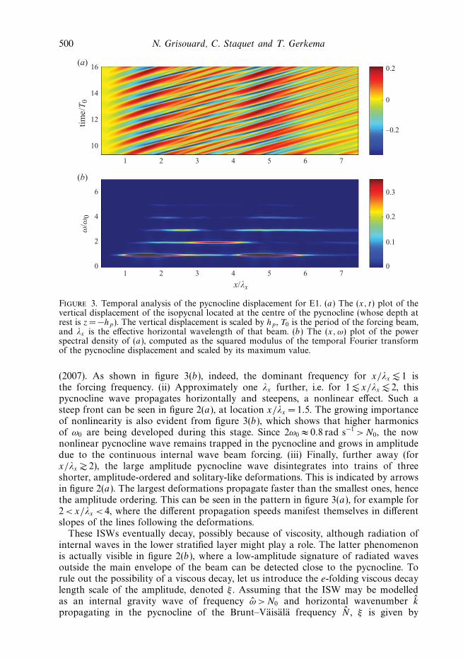
Figure 3. Temporal analysis of the pycnocline displacement for E1. (a) The (x, t) plot of thevertical displacement of the isopycnal located at the centre of the pycnocline (whose depth atrest is z = "hp). The vertical displacement is scaled by hp , T0 is the period of the forcing beam,and !x is the e!ective horizontal wavelength of that beam. (b) The (x, $) plot of the powerspectral density of (a), computed as the squared modulus of the temporal Fourier transformof the pycnocline displacement and scaled by its maximum value.

(2007). As shown in figure 3(b), indeed, the dominant frequency for x/!x " 1 isthe forcing frequency. (ii) Approximately one !x further, i.e. for 1 " x/!x " 2, thispycnocline wave propagates horizontally and steepens, a nonlinear e!ect. Such asteep front can be seen in figure 2(a), at location x/!x = 1.5. The growing importanceof nonlinearity is also evident from figure 3(b), which shows that higher harmonicsof $0 are being developed during this stage. Since 2$0 ) 0.8 rad s"1 >N0, the nownonlinear pycnocline wave remains trapped in the pycnocline and grows in amplitudedue to the continuous internal wave beam forcing. (iii) Finally, further away (forx/!x # 2), the large amplitude pycnocline wave disintegrates into trains of threeshorter, amplitude-ordered and solitary-like deformations. This is indicated by arrowsin figure 2(a). The largest deformations propagate faster than the smallest ones, hencethe amplitude ordering. This can be seen in the pattern in figure 3(a), for example for2 <x/!x < 4, where the di!erent propagation speeds manifest themselves in di!erentslopes of the lines following the deformations.

These ISWs eventually decay, possibly because of viscosity, although radiation ofinternal waves in the lower stratified layer might play a role. The latter phenomenonis actually visible in figure 2(b), where a low-amplitude signature of radiated wavesoutside the main envelope of the beam can be detected close to the pycnocline. Torule out the possibility of a viscous decay, let us introduce the e-folding viscous decaylength scale of the amplitude, denoted / . Assuming that the ISW may be modelledas an internal gravity wave of frequency $ > N0 and horizontal wavenumber kpropagating in the pycnocline of the Brunt–Vaisala frequency N , / is given by


(e.g. Lighthill 1978, p. 272)

/ =1

'

"$

k

#3&

N2 " $2

N3. (3.2)

The ratio $/k is the horizontal phase velocity of the wave and, as we shall see inthe next section, is well approximated by the horizontal phase velocity of the beam$0/kx . The time 2!/$ is the typical temporal width of the ISW and, from figure 3(a),can be estimated as T0/3. Using N = 4 rad s"1 as a typical measure of the Brunt–Vaisala frequency in the pycnocline, we get / =28 m ) 52!x , which is much largerthan the length of the domain L =6 m ) 11!x . Hence, viscosity can be ignored in thisexperiment.

4. How to control the mode number: a ‘far-field’ approach4.1. Heuristic considerations: the modal decomposition

In the present case of a pycnocline of finite thickness, the modal decompositionprovides a simple method to study the structure and characteristics of the full internalgravity wave field that develops over the total water depth. We shall show in thissection that this method also provides a useful heuristical tool to design a numericalexperiment so that mode-1 ISWs develop.

For the sake of simplicity, we will make a rigid-lid approximation. Indeed, in allour experiments, the free-surface displacement never exceeds 0.2 mm, which is twoorders of magnitude smaller than the thickness of the upper homogeneous layer hp .

We briefly recall the principles of the modal decomposition (see e.g. Leblond &Mysak 1978 for detail). When searching for a vertical velocity solution of the linearinviscid Boussinesq equations of the form

w(x, z, t) = W (z) exp i(Kx " 0t) (4.1)

with K > 0 as we are only interested in rightward-propagating waves, it can be shownthat W and K satisfy the eigenvalue problem:

d2W

dz2+ K2 N2(z) " 02

02W = 0, (4.2a)

W |z=0 = W |z="H = 0. (4.2b)

The system of (4.2a) and (4.2b) forms a Sturm–Liouville problem and has an infinitesequence of modes, of eigenfunctions Wn associated with eigenvalues Kn (n beingthe mode number). The general solution for w limited to rightward-propagatingcomponents can therefore be written as

w(x, z, t) =*)

n=0

anWn(z) exp i(Knx " 0t), (4.3)

where the coe"cients (an), n + !, are the amplitude of the modes. Solving (4.2a) and(4.2b) then requires N(z) and 0 as input parameters which determine Wn and Kn foreach mode n (setting K and retrieving 0n would also have been possible). The phasespeeds of each mode are then cn = 0/Kn (or 0n/K).

The case of experiment E1 is now considered to illustrate how we use heuristicallythis method to determine the parameter set that favours the development of a mode-1ISW.


1 2 3 4 50

1

2

3

4

&/%0

c n/v

'

c1/v'

c2/v'

c3/v'

Figure 4. Phase speeds of the first three modes c1, c2 and c3 for experiment E1 computedfrom (4.2a) and (4.2b) as a function of 0 and for N (z) given by (2.1). The phase speeds and0 are scaled by the phase speed v1 and frequency $0 of the wave beam, respectively. Thevertical dashed line marks the location where 0 = N0.

In the work of Akylas et al. (2007), the maximum interfacial displacement isobtained when the horizontal width of the beam (which is well approximated by !x

in our case) matches the horizontal wavelength of the interfacial wave. Since thiswave is forced at the beam frequency, its horizontal phase speed therefore matchesthe horizontal phase speed of the beam. As we now show, when the pycnocline is offinite thickness and weakly nonlinear e!ects have developed, the mode-1 pycnoclinewave also has the same horizontal phase speed as the incoming beam.

To apply the modal decomposition to experiment E1, we assume that an ISW maybe modelled as a superposition of linear internal gravity waves which are trappedwithin the pycnocline, i.e. of frequency comprised between N0 and max(N (z)). Wesolve (4.2a) and (4.2b) with 0 varying and display the phase speeds of the first threemodes c1, c2 and c3 versus 0 in figure 4. The figure shows that the phase speeddecreases as 0 increases, with a sharp transition when 0 = N0 (i.e. for 0/$0 =

'2):

the decrease rate of the phase speeds drops, corresponding to the modes being trappedin the pycnocline. For 0 $ N0, all three phase speeds evolve quasi-linearly, with 0 ,c2 and c3 being nearly constant and distinct from c1. The velocity c1 is very close tothe horizontal phase velocity v1 of the wave beam as 0 increases.

Hence, to select a mode-1 ISW, the internal wave beam should be designed suchthat its horizontal phase speed is close to c1 (computed from modal decompositionfor 0 +]N0, max(N(z))[, N(z) being given). This is how experiment E1 was designed,adjusting also the wave beam amplitude so that a strong deformation is induced inthe pycnocline while ensuring that the beam remains stable.

We will now make the conjecture that in order to excite mode-n ISWs, the horizontalphase speed of the internal wave beam should be within the range of values of thephase speeds of the mode-n internal waves when trapped in the pycnocline (i.e. withfrequency 0 +]N0, max(N (z))[). This conjecture will be verified next.

4.2. Application to the generation of mode-2 and mode-3 internal solitary waves

We now focus on experiments E2 and E3. In figures 5(a) and 5(b), the phase speedsof the first three modes are plotted versus 0 for experiments E2 and E3, respectively.These phase speeds display the same behaviour as for experiment E1, c2 and c3

reaching a nearly constant value as soon as 0 exceeds N0. We find that for 0 > N0,v1 ()1.57 cm s"1) in experiment E2 is closer to c2 ()1.5 cm s"1 as far as we computed


1 2 3 4 50

1

2

4

6

8

(a) (b)

1 2 3 4 501

5

10

15

c n/v

'

&/%0 &/%0

c1/v'

c2/v'

c3/v'

Figure 5. Same as in figure 4 but for experiments (a) E2 and (b) E3.

–0.5

–1.0

–1.51 2 3 4 5

1 2 3

x/!x x/!x

4

2 3 4 5

2 3 4 5

6

–5–10–15–20

–4–8

–12

–0.5

–1.0

–1.5

z/h p

z/h p

(a)

(b)

(c)

(d)

Figure 6. Generation of ISWs by an internal wave beam in experiments E2 and E3. Thisfigure is similar to figure 2 for experiment E1. In (a), mode-2 ISWs develop and a trainwith three visible deformations is highlighted with arrows. In (c), mode-3 ISWs are framed,consisting of a train with two visible deformations. In (b), values range from "5 mm s"1 (blue)to 5 mm s"1 (red) and in (d ), values range from "4 mm s"1 (blue) to 4 mm s"1 (red).

it) in this case. When the modal decomposition is applied to E3, the value of c3

for 0 > N0 ()1 cm s"1) here is the closest to v1 ()0.905 cm s"1). Like E1 with c1,experiments E2 and E3 were actually designed from the computation of c2 and c3

respectively, such that the horizontal phase speed of the wave beam matches c2 in E2and c3 in E3.

Visualisations of the fields similar to figure 2 are displayed in figure 6 for eachexperiment. Figure 6 shows that ISWs develop again from the impact of the wavebeam on the pycnocline (figure 6b, d ). However, the vertical structure of the pycnoclinewave is now a mode 2 for E2 (figure 6a) and a mode 3 in E3 (figure 6c), the numberof visible deformations per train being three in the former case and two in the latter.The amplitude of the mode-3 ISWs is actually rather weak and, as we will see next,very sensitive to viscous e!ects. We verified that the three stages of the process goingfrom a linear to a weakly nonlinear internal wave trapped in the pycnocline, describedin § 3.2, also occur in these two experiments.

In order to validate a posteriori the value of ' we chose, we recall (3.2). For E2, using2!/$ = T0/8 and N = 5.5 rad s"1, we obtain / = 1 m ) 4.3!x , which is now smaller thanthe length of the domain (L = 3 m ) 13!x). For experiment E3, using 2!/$ = T0/6 and


–0.5

–1.0

–1.5

–0.5

–1.5

–2.5

–0.5

–1.5

–2.5

z/h p

z/h p

(a)

(b)

–0.5

–1.0

–1.5

(c)

(d)1.0 1.5 2.0

1.0 1.2 1.4 1.6 1.8 2.0

2.0 2.5 3.0 3.5

2.5 3.0 3.5

4.0

x/!x x/!x

Figure 7. Same as in figure 6 but for experiments E2 (a, b) and E3 (c, d ), magnified aroundthe zones of impact of the internal wave beam in order to emphasise the refraction of thebeam during its propagation in the pycnocline.

N = 6 rad s"1 yields / =0.18 m ) 1.3!x , which is even smaller compared to L (sinceL =1.2 m ) 9!x). The values of $ for E2 and E3 have been estimated from figure 6.The orders of magnitude for / show that for E2 and E3, viscosity plays an importantrole in the decay of the ISWs. Hence, the use for ' of the realistic value 10"6 m2 s"1

would have led to a very quick attenuation of mode-2 ISWs and prevented thedevelopment of mode-3 ISWs, as we verified.

5. How to control the mode number: a ‘near-field’ approachThe approach developed above addresses the ‘far-field’ evolution of the dynamics

within the pycnocline, when nonlinear waves have developed. The approach weconsider now may be referred to as the ‘near-field’ evolution, in the sense that weanalyse the deformation of the pycnocline at the beam impact.

The simple model we shall derive is motivated by a careful inspection of the impactzone of the internal wave beam in experiments E2 and E3, which is magnified infigure 7. The beam is refracted as it gets into the pycnocline, since its frequency andhorizontal wavelength remain unchanged (the dynamics being linear and the changesof the medium occurring along z only) whereas the local Brunt–Vaisala frequencyincreases. We shall see that conditions for optimal forcing of the pycnocline wave bythe beam can be derived, which also set the vertical structure (i.e. mode number) ofthe pycnocline wave.

The model is based on three approximations: (i) we focus on the initial phase ofwave generation in the pycnocline, so that the dynamics may be assumed linear;(ii) we also consider a simple plane wave instead of a wave beam; (iii) we assumethat the profile of the Brunt–Vaisala frequency is a piecewise continuous functionconsisting of three parts, namely

N23L(z) =

*++++,

++++-

N20 , for " H ! z < "hp " &p

2,

N2i , for " hp " &p

2! z ! "hp +

&p

2,

0, for " hp +&p

2< z ! 0,

(5.1)

where Ni is the Brunt–Vaisala frequency within the pycnocline. The value of Ni hasbeen chosen in order to preserve the phase shift between the induced displacements


(i

(0

!x /2

!p

(a) (b)

(i

(0

!x

!p

Figure 8. Sketches illustrating the conditions for the generation of mode-2 (a) and mode-3(b) internal waves trapped in a pycnocline using the linear, three-layer model presented in§ 5. The shaded area is the pycnocline, the thick dashed lines represent isophases of thedisplacement separated by a distance !x/2 (phase shift !) and the dotted lines sketch thedisplacements induced by the plane wave in the pycnocline, highlighting the selected verticalstructure.

of the top and bottom of the pycnocline. In other words, let us assume that in ournumerical experiments, an internal wave characteristic impinges on the bottom ofthe pycnocline at a location x0 and is refracted until being reflected against the topof the pycnocline at the location x0 + "x. Our three-layer model is designed suchthat the locations x0 and x0 + "x are preserved, although the characteristics are nowpiecewise straight lines. The slope of a characteristic is equal to

&$2

0/(N2(z) " $2

0) and"x is computed by integrating the path of a characteristic between the boundaries ofthe pycnocline, which we set to be at depths z1 = "hp " &p/2 and z2 = "hp + &p/2:

"x =

. z2

z1

dz

/N2(z) " $2

0

$20

. (5.2)

In the case of a pycnocline characterised by the constant Brunt–Vaisala frequency Ni ,this expression reduces to "x = &p

&(N2

i " $20)/$2

0. Matching these two expressionsthen leads to the following expression for Ni:

N2i = $2

0 +$2

0

&2p

0. z2

z1

dz

/N2(z) " $2

0

$20

12

. (5.3)

We show that a Bragg-like resonance condition based on simple geometricarguments can be obtained for the selection of the mode. At depth z = "hp " &p/2,upon entering the pycnocline, the angle of propagation of the energy of the planewave is changed from %0 to %i = arcsin($0/Ni) < %0, due to refraction. Leaving asidethe mode-1 case, which does not seem to be tractable with the present approach, wenow distinguish the two cases we investigate, starting with the forcing of a mode-2pycnocline wave.

Two isophases of the incident plane wave are plotted in figure 8(a) as well as twoisopycnals at the top and bottom of the pycnocline. If the horizontal wavelength ofthe plane wave !x is such that !x/2 = "x, the induced displacements of the top andbottom of the pycnocline are opposite in phase (phase shift of !), making the verticalstructure of the refracted wave in the pycnocline similar to that of a mode-2 internalwave. Figure 8(a) only displays wave characteristics until one reaches the top of thepycnocline but the wave characteristics can be drawn further along the pycnoclinewithout altering the pattern of a mode-2 internal wave. The subsequent steps are


Experiment E2 E3

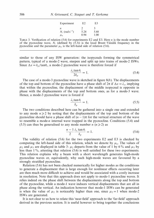
n 2 3Ni (rad s"1) 5.24 5.68µn 0.94 1.00

Table 3. Verification of relation (5.6) for experiments E2 and E3. Here n is the mode numberof the pycnocline wave, Ni (defined by (5.3)) is the local Brunt–Vaisala frequency in thepycnocline and the parameter µn is the left-hand side of relation (5.6).

similar to those of any ISW generation: the isopycnals forming the symmetricalpattern, typical of a mode-2 wave, steepen and split up into trains of mode-2 ISWs.Since "x = &p/tan%i , a mode-2 pycnocline wave is therefore forced if

!xtan %i

2&p

= 1. (5.4)

The case of a mode-3 pycnocline wave is sketched in figure 8(b). The displacementsof the top and bottom of the pycnocline have a phase shift of 2! if "x = !x , implyingthat within the pycnocline, the displacement of the middle isopycnal is opposite inphase with the displacements of the top and bottom ones, as for a mode-3 wave.Hence, a mode-3 pycnocline wave is forced if

!xtan %i

&p

= 1. (5.5)

The two conditions described here can be gathered into a single one and extendedto any mode n $ 2 by noting that the displacements of the top and bottom of thepycnocline should have a phase shift of (n " 1)! for the vertical structure of the waveto resemble a mode-n internal wave trapped in the pycnocline. Conditions (5.4) and(5.5) can thus be generalised to any mode number n (n $ 2) as

n " 1

2

!x tan %i

&p

= 1. (5.6)

The validity of relation (5.6) for the two experiments E2 and E3 is checked bycomputing the left-hand side of this relation, which we denote by µn. The values ofµ2 and µ3 are displayed in table 3: µ2 departs from the value of 1 by 6 % and µ3 byless than 1 %, attesting that relation (5.6) is well satisfied for these two experiments.This relation explains why a beam with a short wavelength generates high-modepycnocline waves or, equivalently, why such high-mode waves are favoured by astrongly stratified pycnocline.

Relation (5.6) has not been checked numerically for higher modes as the conditionsto generate a displacement that is large enough for nonlinear e!ects occurring laterare then much more di"cult to achieve and would be associated with a costly increasein resolution. Note that this approach does not apply to mode-1 pycnocline waves. Itrelies indeed on the phase shift between the displacements along the top and bottomof the pycnocline, while a mode-1 wave induces vertical displacements that are all inphase along the vertical. An indication however that mode-1 ISWs can be generatedis when the value of µ2 is noticeably higher than one, since µ2 = 1 when mode-2ISWs are generated.

It is not clear to us how to relate this ‘near-field’ approach to the ‘far-field’ approachderived in the previous section. It is useful however to bring together the conclusions


of the two approaches. Writing v1 = cn on the one hand, and relation (5.6) on theother hand, allows one to derive an approximate analytical expression for cn, namely

cn =&p

&N2

i " $20

!(n " 1). (5.7)

This is obtained by expressing (5.6) in terms of v1 (= $0!x/2!), writing the dispersion

relation as $0 =Ni sin %i and therefore Ni cos %i =&

N2i " $2

0. As Ni , $0 for the threeexperiments, (5.7) can be simplified to cn = &pNi/(!(n " 1)). Numerical estimate ofcn given by (5.7) for the parameters of table 2 yields c2 ) 1.66 cm s"1 for E2 andc3 ) 0.901 cm s"1 for E3, which is in good agreement with the values given in § 4.2.

6. Discussion6.1. Bandwidths of the selection conditions

This paper aims at determining optimal conditions to generate mode-n ISWs.However, the bandwidths of these conditions have not been discussed. In otherwords, when for a given situation, µn < 1 <µn+1 and/or cn < v1 <cn+1 in the trappedregime, it is yet to be determined whether ISWs develop at all and, if they do,which of the two n or n + 1 modes would preferentially develop and what wouldbe their amplitudes. From a qualitative point of view, the answer must depend onseveral parameters, such as the ratio |cn " v1 |/|v1 " cn+1| in the trapped regime or anyquantity comparing the distances between v1 and the di!erent phase speeds in thatregime. From a quantitative point of view, the computation of the amplitude of thetrapped modes would provide a precise answer but would be quite involved as thenonlinear nature of these waves implies that the motion cannot be easily projectedon an orthogonal basis of linear wave modes at a given frequency. The projection ofthe motion on an orthogonal basis of nonlinear modes would require to know whichmodel (such as a high-order KdV model) describes it accurately, which has not beendone for the present paper.

To get some indication of the bandwidths of the selection conditions (i.e. of thenear-field and far-field conditions), we rather performed another numerical experiment(not shown). This experiment involves a beam, for which v1 is the same as in E1but the stratification profile is the same as in E2. From the near-field condition (5.4),one finds µ2 = 2.17 > 1, which implies that mode-1 ISWs can be generated (as thenear-field condition does not apply to mode-1 ISWs, it is not possible to be morespecific). Regarding the far-field condition, figure 5(a) for E2 shows that v1 is halfwaybetween c1 and c2 in the trapped regime (since v1 for E1 is 2.3 times larger than forE2). Therefore, we are in an intermediate regime.

Observation of the pycnocline motion in this experiment shows a dominant mode-1pattern for the ISWs, with an amplitude of the induced isopycnal displacementof about 3 mm. Superposed on this isopycnal displacement is a secondary pattern,typical of mode-2 ISWs. Mode-2 isopycnal displacements (measured with respect tothe displacements, already induced by the mode-1 ISWs) are less than 1 mm. On thebasis of this crude estimate, we infer that the two bandwidths for the far-field selectionconditions overlap but the bandwidth for the selection of mode-1 ISWs seems to belarger than that for mode-2 ISWs.

Two conjectures can be proposed based on this example: first, that when inan intermediate case, ISWs can be generated and the bandwidths of the selectionconditions for each mode number can overlap; second, that the lower the mode of


0 0.2 0.4 0.6 0.8 1.0 1.2 1.4 1.6

–4000

–3500

–3000

–2500

–2000

–1500

–1000

–500

0

N (! 10!2 rad s!1)

z (m)

Figure 9. Typical stratification observed in the Bay of Biscay in mid-to-late summer.

the ISWs is, the broader the bandwidth of its selection condition might be. Theseconjectures both seemed to be verified in a few other numerical tests that helped usto derive our selection conditions.

6.2. Applicability of the selection conditions to an oceanic setting

This paper addresses fundamental aspects of the generation of ISWs by an internalwave beam. However, let us recall that this problem was motivated by oceanicobservations. In this section, we apply the selection conditions to the more realisticcontext of the Bay of Biscay and investigate whether these conditions can correctlypredict the observations. (As found by New & Pingree 1990, 1992, local generation inthe Bay of Biscay is associated with mode-1 ISWs.) We will also show that rotationcan be easily introduced in the far-field and near-field approaches.

The reference stratification profile we consider is a typical profile observed inthe Bay of Biscay in mid-to-late summer, when the seasonal pycnocline is bestdeveloped and when local generation is observed. This reference profile (displayedin figure 9) is characterised by a strong seasonal pycnocline whose maximal valueis 1.6 & 10"2 rad s"1 at 58 m depth. Note the presence of a permanent pycnoclinecorresponding to increased values of N between roughly 400 m and 2000 m depth.This profile has been deduced from data described in New (1988) and Pingree & New(1991). The dominant forcing frequency in the Bay of Biscay is the semidiurnal tideof frequency $BB = 1.41 & 10"4 rad s"1, corresponding to a period of 12.42 h.

Let us see how the far-field condition applies to the configurations just described. Inorder to compute the phase speeds of the di!erent internal wave modes, we introducerotation in (4.2a),

d2W

dz2+ K2 N2(z) " 02

02 " f 245o

W (z) = 0, (6.1)

where f45o = 10"4 rad s"1 is the Coriolis parameter at a latitude of 45o. The rest ofthe procedure is as in § 4.


5 10 15 20 25 300

0.5

1.0

1.5

2.0

2.5

3.0

3.5

&/%BB

Phas

e sp

eed

(m s

!1)

c1

c2

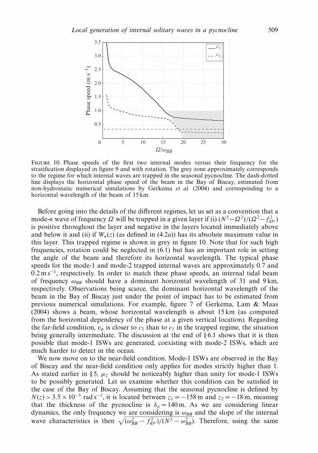
Figure 10. Phase speeds of the first two internal modes versus their frequency for thestratification displayed in figure 9 and with rotation. The grey zone approximately correspondsto the regime for which internal waves are trapped in the seasonal pycnocline. The dash-dottedline displays the horizontal phase speed of the beam in the Bay of Biscay, estimated fromnon-hydrostatic numerical simulations by Gerkema et al. (2004) and corresponding to ahorizontal wavelength of the beam of 15 km.

Before going into the details of the di!erent regimes, let us set as a convention that amode-n wave of frequency 0 will be trapped in a given layer if (i) (N2"02)/(02"f 2

45o )is positive throughout the layer and negative in the layers located immediately aboveand below it and (ii) if Wn(z) (as defined in (4.2a)) has its absolute maximum value inthis layer. This trapped regime is shown in grey in figure 10. Note that for such highfrequencies, rotation could be neglected in (6.1) but has an important role in settingthe angle of the beam and therefore its horizontal wavelength. The typical phasespeeds for the mode-1 and mode-2 trapped internal waves are approximately 0.7 and0.2 m s"1, respectively. In order to match these phase speeds, an internal tidal beamof frequency $BB should have a dominant horizontal wavelength of 31 and 9 km,respectively. Observations being scarce, the dominant horizontal wavelength of thebeam in the Bay of Biscay just under the point of impact has to be estimated fromprevious numerical simulations. For example, figure 7 of Gerkema, Lam & Maas(2004) shows a beam, whose horizontal wavelength is about 15 km (as computedfrom the horizontal dependency of the phase at a given vertical location). Regardingthe far-field condition, v1 is closer to c2 than to c1 in the trapped regime, the situationbeing generally intermediate. The discussion at the end of § 6.1 shows that it is thenpossible that mode-1 ISWs are generated, coexisting with mode-2 ISWs, which aremuch harder to detect in the ocean.

We now move on to the near-field condition. Mode-1 ISWs are observed in the Bayof Biscay and the near-field condition only applies for modes strictly higher than 1.As stated earlier in § 5, µ2 should be noticeably higher than unity for mode-1 ISWsto be possibly generated. Let us examine whether this condition can be satisfied inthe case of the Bay of Biscay. Assuming that the seasonal pycnocline is defined byN(z) > 3.5 & 10"3 rad s"1, it is located between z1 = "158 m and z2 = "18 m, meaningthat the thickness of the pycnocline is &p = 140 m. As we are considering lineardynamics, the only frequency we are considering is $BB and the slope of the internalwave characteristics is then

&($2

BB " f 245o )/(N2 " $2

BB). Therefore, using the same


notation as in § 5, "x now has to verify the following condition:

"x =

. z2

z1

dz

/N2(z) " $2

BB

$2BB " f 2

45o

= &p

/N2

i " $2BB

$2BB " f 2

45o

. (6.2)

Then, Ni is defined by

N2i = $2

BB +$2

BB " f 245o

&2p

0. z2

z1

dz

/N2(z) " $2

BB

$2BB " f 2

45o

12

. (6.3)

We find Ni = 8.4 & 10"3 rad s"1. Once rotation is also included in the definition of%i , the procedure is the same as in § 5. In order to satisfy µ2 = 1, the wave beamshould have a dominant horizontal wavelength of 24 km, which is higher than thedominant horizontal wavelength of the beam in the Bay of Biscay as estimatedearlier. Moreover, in order to satisfy µ3 = 1, the wave beam should have a horizontalwavelength of 12 km. The near-field condition therefore predicts here that we arein an intermediate case between the generation of mode-2 and mode-3 ISWs. Theseconsiderations lead us to the conclusion that this simple model is quantitatively lesssuitable than the far-field approach when it comes to realistic conditions, one possiblereason being the large uncertainties on the parameters that enter the model.

In comparison, the arguments on which the far-field approach is based are muchmore robust: for a given mode number n, trapped pycnocline waves with di!erentfrequencies propagate with phase speeds that are close to each other, which is thereforethe approximate propagation speed of any mode-n ISW trapped in the pycnocline.A beam (or any other disturbance) should therefore have a horizontal phase speedthat is close to this value to e"ciently force mode-n ISWs (provided that the forcingis strong enough for nonlinear e!ects to develop within its direct range).

7. ConclusionWe addressed the local generation of ISWs, when an internal wave beam impinges

on a pycnocline. Nonlinear, non-hydrostatic numerical experiments were conductedfor this purpose, the vertical density profile being continuous and made of a lowerlayer with constant value N0 of the Brunt–Vaisala frequency, a pycnocline of finitethickness and a thin homogeneous upper layer. This work complements previoustheoretical (Gerkema 2001; Akylas et al. 2007) and experimental (Delisi & Orlanski1975) studies in which the thickness of the pycnocline was vanishingly small (i.e. aninterface).

We showed that ISWs can be generated and that the finite thickness of thepycnocline, whose role is fundamental, allows di!erent vertical modes to be excited,depending on the parameters. We ran numerical experiments showing that modes-1, -2or -3 internal solitary waves can develop. We next proposed two di!erent approachesto predict the conditions of occurrence of mode-n internal solitary waves.

In the ‘far-field’ approach, that is, when harmonics of the forcing frequency haveappeared, we showed that the observed mode-n weakly nonlinear pycnocline waveshave the same horizontal phase speed as the incident wave beam. We demonstratedthis result heuristically by using a modal decomposition based upon the actualdensity profile and a frequency of value higher than N0. This result allowed us todesign numerical experiments so that a mode-1, -2 or -3 pycnocline wave develops, the


density jump across the pycnocline increasing with the mode number (or equivalently,the horizontal wavelength of the wave beam decreasing with the mode number).

One might wonder why the phase speed of a beam should be matched with thephase speed of trapped waves, which are physically some distance away from thebeam. We observed in § 3.2 that the evolution towards ISWs actually takes one or twowavelengths only, a much shorter distance than for weakly nonlinear waves describede.g. by a KdV model. This is very likely due to the large amplitude of the forcing,which allows the development of nonlinear structures in its vicinity that propagatewith the same speed as the forcing phase speed.

The ‘near-field’ approach consists of deriving simple geometrical conditions ensuringthat a mode-n wave develops at the beam impact (the model holds for n $ 2 only). Inthis approach, the dynamics is linear, a simple plane wave is considered in place ofa wave beam and a piecewise three-layer stratification is assumed. We showed thata mode-n wave is forced if a simple relation is satisfied which involves the thicknessof the pycnocline, the angle of the refracted internal wave in the pycnocline andthe horizontal wavelength of this wave. In spite of its simplicity, this model gavea good quantitative agreement with our numerical data for n $ 2. It explains whya beam with a short wavelength generates high-mode waves or, equivalently, whysuch high-mode waves are favoured by a strongly stratified pycnocline. When relatedto the far-field approach, this model provides a simple analytical expression for thephase speed of a mode-n ISW.

We discussed the more general situation in which the wave beam has an intermediatephase speed between those of modes n and n + 1. We conjectured from an examplethat both modes could be selected in this case and that the lower the mode numberis, the larger is its bandwidth. The computation of the amplitude of those modesis necessary to answer precisely this problem. This requires solving the nonlinearnon-hydrostatic Boussinesq equations forced by the wave beam, a rather involvedtask.

The predictions of the two selection conditions derived in this paper were eventuallyexamined in the more realistic context of the Bay of Biscay, in which mode-1 ISWsare observed. The far-field approach predicts a situation that is intermediate betweenthe selection of mode-1 and mode-2 ISWs and an agreement with the observationsis therefore possible (for more details, see Grisouard & Staquet 2010). In contrast,the near-field approach does not seem to be quantitatively reliable when appliedto this realistic configuration, as it predicts a situation that is intermediate betweenthe selection of mode-2 and mode-3 ISWs. However, the application of the latterselection rule requires several simplifications, which leads to strong uncertainties inthe parameters that enter the model.

Independent of the validity of these selection rules, it remains to investigate whetherthe mechanism leading to the generation of ISWs remains valid in a real ocean. Thebeams may have a three-dimensional structure and the generation process as awhole might be sensitive to perturbations from other structures such as eddies orother internal waves. The latter is the subject of a study by Grisouard & Staquet(2010).

We thank the experimental team for having shared their early results, especiallyL. Gostiaux, M. Mercier and M. Mathur. M. Mathur is also acknowledged for hishelp during the revision of this paper. The detailed comments of the anonymousreferees greatly helped to improve this article. N.G. is supported by a grant from theDirection Generale de l’Armement. This work has been supported by ANR contracts


TOPOGI-3D (05-BLAN-0176) and PIWO (08-BLAN-0113). Numerical experimentswere performed on the French supercomputer centre IDRIS, through contracts 070580and 080580.

REFERENCES

Akylas, T. R., Grimshaw, R. H. J., Clarke, S. R. & Tabaei, A. 2007 Reflecting tidal wave beamsand local generation of solitary waves in the ocean thermocline. J. Fluid Mech. 593, 297–313.

Azevedo, A., da Silva, J. C. B. & New, A. L. 2006 On the generation and propagation of internalsolitary waves in the southern Bay of Biscay. Deep-Sea Res. I 53, 927–941.

Delisi, D. P. & Orlanski, I. 1975 On the role of density jumps in the reflexion and breaking ofinternal gravity waves. J. Fluid Mech. 69, 445–464.

Gerkema, T. 2001 Internal and interfacial tides: Beam scattering and local generation of solitarywaves. J. Mar. Res. 59, 227–255.

Gerkema, T., Lam, F.-P. A. & Maas, L. R. M. 2004 Internal tides in the Bay of Biscay: Conversionrates and seasonal e!ects. Deep-Sea Res. II 51, 2995–3008.

Gostiaux, L. & Dauxois, T. 2007 Laboratory experiments on the generation of internal tidal beamsover steep slopes. Phys. Fluids 19 (2), 028102.

Grisouard, N. & Staquet, C. 2010 Numerical simulations of the local generation of internalsolitary waves in the Bay of Biscay. Nonlinear Process. Geophys. 17, 575–584.

Helfrich, K. R. & Melville, W. K. 2006 Long nonlinear internal waves. Annu. Rev. Fluid Mech.38, 395–425.

Konyaev, K., Sabinin, K. & Serebryany, A. 1995 Large-amplitude internal waves at the MascareneRidge in the Indian Ocean. Deep-Sea Res. I 42, 2075–2081.

Leblond, P. H. & Mysak, L. A. 1978 Waves in the Ocean . Elsevier.Lighthill, J. 1978 Waves in Fluids . Cambridge University Press.Marshall, J., Hill, C., Perelman, L. & Adcroft, A. 1997 Hydrostatic, quasi-hydrostatic, and

nonhydrostatic ocean modeling. J. Geophys. Res. 102, 5733–5752.Mathur, M. & Peacock, T. 2009 Internal wave beam propagation in non-uniform stratifications.

J. Fluid Mech. 639 (1), 133–152.Mauge, R. & Gerkema, T. 2008 Generation of weakly nonlinear nonhydrostatic internal tides

over large topography: a multi-modal approach. Nonlinear Process. Geophys. 15, 233–244.

New, A. L. 1988 Internal tidal mixing in the Bay of Biscay. Deep-Sea Res. 35 (5), 691–709.New, A. L. & Pingree, R. D. 1990 Large-amplitude internal soliton packets in the central Bay of

Biscay. Deep-Sea Res. 37 (3), 513–524.New, A. L. & Pingree, R. D. 1992 Local generation of internal soliton packets in the central Bay

of Biscay. Deep-Sea Res. 39 (9), 1521–1534.New, A. L. & da Silva, J. C. B. 2002 Remote-sensing evidence for the local generation of internal

soliton packets in the central Bay of Biscay. Deep-Sea Res. I 49, 915–934.Ostrovsky, L. A. & Stepanyants, Y. A. 1989 Do internal solitons exist in the ocean? Rev. Geophys.

27, 293–310.Pingree, R. D. & New, A. L. 1991 Abyssal penetration and bottom reflection of internal tidal

energy in the Bay of Biscay. J. Phys. Oceanogr. 21, 28–39.da Silva, J. C. B., New, A. L. & Azevedo, A. 2007 On the role of SAR for observing ‘local

generation’ of internal solitary waves o! the Iberian Peninsula. Can. J. Remote Sens. 33 (5),388–403.

da Silva, J. C. B., New, A. L. M. & Magalhaes, J. M. 2009 Internal solitary waves in theMozambique Channel: Observations and interpretation. J. Geophys. Res. 114, C05001.

Staquet, C., Sommeria, J., Goswami, K. & Mehdizadeh, M. 2006 Propagation of the Internal Tidefrom a Continental Shelf: Laboratory and Numerical Experiments. In Sixth InternationalSymposium on Stratified Flows, Perth, Australia, pp. 539–544.

Thomas, N. H. & Stevenson, T. N. 1972 A similarity solution for viscous internal waves. J. FluidMech. 54, 495–506.


Thorpe, S. A. 1987 Reflection of internal waves from a uniform slope. J. Fluid Mech. 178, 279–302.Thorpe, S. A. 1998 Nonlinear reflection of internal waves at a density discontinuity at the base of

the mixed layer. J. Phys. Oceanogr. 28, 1853–1860.Zhang, H. P., King, B. & Swinney, H. L. 2007 Experimental study of internal gravity waves

generated by supercritical topography. Phys. Fluids 19 (9), 096602.Zhang, K. Q. & Marotzke, J. 1999 The importance of open-boundary estimation for an Indian

Ocean GCM-data synthesis. J. Mar. Res. 57 (2), 305–334.

generation of internal solitary waves in a pycnocline by ... · theory and to study isws of large...

Documents