low-ranksemideﬁnite programming: theoryand...

Foundations and TrendsR© in OptimizationVol. 2, No. 1-2 (2015) 1–156c© 2016 A. Lemon, A. M.-C. So, Y. YeDOI: 10.1561/2400000009

Low-Rank Semidefinite Programming:Theory and Applications

Alex Lemon Stanford University

[email protected]

Anthony Man-Cho So The Chinese University of Hong Kong

[email protected]

Yinyu YeStanford [email protected]

Contents

1 Introduction 21.1 Low-rank semidefinite programming . . . . . . . . . . . . 21.2 Outline . . . . . . . . . . . . . . . . . . . . . . . . . . . . 4

I Theory 5

2 Exact Solutions and Theorems about Rank 62.1 Introduction . . . . . . . . . . . . . . . . . . . . . . . . . 62.2 Rank reduction for semidefinite programs . . . . . . . . . 62.3 Rank and uniqueness . . . . . . . . . . . . . . . . . . . . 182.4 Rank and sparsity . . . . . . . . . . . . . . . . . . . . . . 23

3 Heuristics and Approximate Solutions 303.1 Introduction . . . . . . . . . . . . . . . . . . . . . . . . . 303.2 Nonlinear-programming algorithms . . . . . . . . . . . . . 313.3 The nuclear-norm heuristic . . . . . . . . . . . . . . . . . 323.4 Rounding methods . . . . . . . . . . . . . . . . . . . . . . 39

ii

II Applications 53

4 Trust-Region Problems 544.1 SDP relaxation of a trust-region problem . . . . . . . . . . 554.2 The simple trust-region problem . . . . . . . . . . . . . . 584.3 Linear equality constraints . . . . . . . . . . . . . . . . . . 584.4 Linear inequality constraints . . . . . . . . . . . . . . . . . 604.5 Ellipsoidal quadratic inequality constraints . . . . . . . . . 81

5 QCQPs with Complex Variables 845.1 Introduction . . . . . . . . . . . . . . . . . . . . . . . . . 845.2 Rank of SDP solutions . . . . . . . . . . . . . . . . . . . 855.3 Connection to the S-procedure . . . . . . . . . . . . . . . 915.4 Applications to signal processing . . . . . . . . . . . . . . 98

Acknowledgments 108

Appendices 109

A Background 110A.1 Linear algebra . . . . . . . . . . . . . . . . . . . . . . . . 110A.2 Optimization . . . . . . . . . . . . . . . . . . . . . . . . . 122

B Linear Programs and Cardinality 131B.1 Sparsification for linear programs . . . . . . . . . . . . . . 132B.2 Cardinality and uniqueness for linear programs . . . . . . . 137

C Technical Probability Lemmas 140C.1 Convex combinations of chi-squared random variables . . . 140C.2 The bivariate normal distribution . . . . . . . . . . . . . . 144

References 149

ii

Abstract

Finding low-rank solutions of semidefinite programs is important inmany applications. For example, semidefinite programs that arise asrelaxations of polynomial optimization problems are exact relaxationswhen the semidefinite program has a rank-1 solution. Unfortunately,computing a minimum-rank solution of a semidefinite program is anNP-hard problem. In this paper we review the theory of low-ranksemidefinite programming, presenting theorems that guarantee the ex-istence of a low-rank solution, heuristics for computing low-rank solu-tions, and algorithms for finding low-rank approximate solutions. Thenwe present applications of the theory to trust-region problems and sig-nal processing.

A. Lemon, A. M.-C. So, Y. Ye. Low-Rank Semidefinite Programming:Theory and Applications. Foundations and TrendsR© in Optimization, vol. 2,no. 1-2, pp. 1–156, 2015.DOI: 10.1561/2400000009.

Introduction

1

1Introduction

1.1 Low-rank semidefinite programming

A semidefinite program (SDP) is an optimization problem of the form

minimize C •Xsubject to Ai •X = bi, i = 1, . . . ,m

X � 0.

(SDP)

The optimization variable is X ∈ Sn, where Sn is the set of all n × nsymmetric matrices, and the problem data are A1, . . . , Am, C ∈ Sn andb ∈ Rm. The trace inner product of A,B ∈ Rm×n is

A •B = tr(ATB) =m∑i=1

n∑j=1

AijBij .

The constraint X � 0 denotes a generalized inequality with respect tothe cone of positive-semidefinite matrices, and means that X is positivesemidefinite: that is, zTXz ≥ 0 for all z ∈ Rn. We can write (SDP)more compactly by defining the operator A : Sn → Rm such that

A(X) =

A1 •X

...Am •X

.2

1.1. Low-rank semidefinite programming 3

Using this notation we can express (SDP) as

minimize C •Xsubject to A(X) = b

X � 0.

The dual problem of (SDP) is

maximize bTy

subject to∑mi=1 yiAi + S = C

S � 0,

(SDD)

where the optimization variables are y ∈ Rm and S ∈ Sn. We can write(SDD) more succinctly as

maximize bTy

subject to A∗(y) + S = C

S � 0,

where the adjoint operator A∗ : Rm → Sn is given by

A∗(y) =m∑i=1

yiAi.

We do not attempt to give a general exposition of the theory of semidef-inite programming in this paper – an excellent survey is provided byVandenberghe and Boyd [96]. The preceding remarks are only meantto establish our particular conventions for talking about SDPs. Addi-tional results about SDPs are given in Appendix A, which presentsthose aspects of the theory that are most relevant for our purposes.

Semidefinite programs can be solved efficiently using interior-point algorithms. However, such algorithms typically converge to amaximum-rank solution [45], and in many cases we are interested infinding a low-rank solution. For example, it is well known that everypolynomial optimization problem has a natural SDP relaxation, andthis relaxation is exact when it has a rank-1 solution. (We include thederivation of this important result in Appendix A for completeness.)Unfortunately, finding a minimum-rank solution of an SDP is NP-hard:a special case of this problem is finding a minimum-cardinality solution

4 Introduction

of a system of linear equations, which is known to be NP-hard [36]. Inthis paper we review approaches to finding low-rank solutions and ap-proximate solutions of SDPs, and present some applications in whichlow-rank solutions are important.

1.2 Outline

Chapter 2 discusses reduced-rank exact solutions of SDPs and theo-rems about rank. We give an efficient algorithm for reducing the rankof a solution. Although the algorithm may not find a minimum-rank so-lution, it often works well in practice, and we can prove a bound on therank of the solution returned by the algorithm. Then we give a theoremrelating the uniqueness of the rank of a solution to the uniqueness ofthe solution itself, and show how to use this theorem for sensor-networklocalization. The chapter concludes with a theorem that allows us todeduce the existence of a low-rank solution from the sparsity structureof the coefficients.

Because finding a minimum-rank solution of an SDP is NP-hard,we do not expect to arrive at an algorithm that accomplishes this taskin general. However, there are many heuristics for finding low-ranksolutions that often perform well in practice; we discuss these methodsin Chapter 3. We also present rounding methods, in which we find alow-rank approximate solution that is close to a given exact solution insome sense. One of the rounding methods that we discuss is the famousGoemans-Williamson algorithm [39]; if the unique-games conjecture istrue, then this algorithm achieves the best possible approximation ratiofor the maximum-cut problem [57, 58].

The paper concludes with two chapters covering applications ofthe theoretical results to trust-region problems and signal processing.There are three appendices: the first gives background information, andestablishes our notation; the second reviews some classical results aboutlinear programming that we generalize to semidefinite programming inChapter 2; and the last contains technical probability lemmas that areused in our analysis of rounding methods.

Part I

Theory

2Exact Solutions and Theorems about Rank

2.1 Introduction

In this chapter we discuss exact reduced-rank solutions and theoremsabout rank. We begin by extending classical results about the cardinal-ity of solutions of linear programs (reviewed in Appendix B) to resultsabout the rank of solutions of semidefinite programs. Then we presenta theorem that allows us to use the sparsity structure of the coefficientsof an SDP to guarantee the existence of a low-rank solution.

2.2 Rank reduction for semidefinite programs

We now generalize the well-known analysis of sparsification for lin-ear programs to rank reduction for semidefinite programs. (The corre-sponding sparsification algorithm for LPs is described in Appendix B;our presentation of the corresponding rank-reduction algorithm forSDPs is deliberately similar.) The main result is Theorem 2.1, whichguarantees the existence of a solution of (SDP) whose rank r satis-fies r(r + 1)/2 ≤ m, where m is the number of linear equality con-straints. This bound was independently discovered by Barvinok [3] andPataki [76].

6

2.2. Rank reduction for semidefinite programs 7

Suppose we are given a solution X of (SDP), and we want to findanother solution X+ with rank(X+) < rank(X). If we had an effi-cient method for this problem that worked on every solution that doesnot have minimum rank, then we could find a minimum-rank solutionby applying this rank-reduction method at most n times. However, weknow that the problem of finding a minimum-rank solution of (SDP) isNP-hard. Thus, we do not expect to find an efficient rank-reduction al-gorithm that always works. Nonetheless, we still hope to find a methodthat often performs well in practice. We begin by making the followingassumption:

null(X+) ⊃ null(X), (2.1)

where null(X) = {z ∈ Rn |Xz = 0} is the nullspace of X. Observe thestrong similarity between this assumption, and the assumption (B.1)that forms the basis for the standard LP-sparsification algorithm: inthe LP case, we assume that if a component of x is zero, then thecorresponding component of x+ is also zero; in the SDP case, we assumethat if X has zero gain in some direction, then X+ also has zero gainin that direction. (Here we interpret a nonzero vector being in thenullspace of a matrix as meaning that the matrix has zero gain inthe direction of the vector.) The following example shows that thisassumption can yield suboptimal results in some cases.

Example 2.1. Consider the SDP feasibility problem

Xii +Xnn = 1, i = 1, . . . , n− 1Xij = 0, 1 ≤ i < j ≤ nX � 0,

and suppose we are given the solution X = diag(1, . . . , 1, 0). If weassume that null(X+) ⊃ null(X), then we have that en ∈ null(X+)because en ∈ null(X). (Here en is the nth standard basis vector inRn: that is, the vector of length n whose nth component is equal to1, and whose other components are all equal to 0.) This implies thatX+nn = eT

nX+en = 0. Then the equality constraint X+

ii + X+nn = 1

implies that X+ii = 1 for i = 1, . . . , n − 1. Therefore, we have that

X+ = X, and we are unable to reduce the rank of X. However, X is not

8 Exact Solutions and Theorems about Rank

a minimum-rank solution of the feasibility problem: rank(X) = n− 1,but X = diag(0, . . . , 0, 1) is a solution with rank(X) = 1.

Example 2.1 shows that the assumption in (2.1) may not only leadto suboptimal results, but may even lead to arbitrarily poor results:for every positive integer n, there is an instance of (SDP) and a cor-responding initial solution such that our algorithm returns a solutionwhose rank is n− 1 times the rank of a minimum-rank solution. How-ever, because we do not expect to find an algorithm that works on everyinstance of (SDP), we need to make a suboptimal assumption at somepoint. Moreover, we will see that the assumption in (2.1) allows us toderive an algorithm that often works well, and has some performanceguarantees.

We have stated our assumption as null(X+) ⊃ null(X). Althoughthis statement is clear and intuitive, a different formulation will proveuseful in the development of our algorithm. Let r = rank(X). SinceX is positive semidefinite, there exists a matrix V ∈ Rn×r such thatX = V V T. Then assumption (2.1) is equivalent to assuming that X+

has the formX+ = V (I + α∆)V T,

where we think of ∆ ∈ Sn as an update direction, and α ∈ R as a stepsize. We will also sometimes find it convenient to write X+ as

X+ = X + αV∆V T.

The fact that the proposed reformulation is equivalent to (2.1) is aconsequence of Proposition A.1.

We want to choose α and ∆ such that X+ is a solution of (SDP),and rank(X+) < rank(X). Since the rank of X+ is strictly less thanthat of X, we must have that X+ 6= X, and hence that α 6= 0.

• In order to maintain optimality, we require that

C •X+ = C •X.

Substituting in X+ = X + αV∆V T and simplifying, we obtainthe condition

(V TCV ) •∆ = 0.


• We also need X+ to satisfy the equality constraints

Ai •X+ = bi, i = 1, . . . ,m.

Substituting in our expression for X+ and simplifying gives theconditions

(V TAiV ) •∆ = 0, i = 1, . . . ,m.

For convenience we define the mapping AV : Sr → Rm such that

AV (∆) = A(V∆V T) =

(V TA1V ) •∆

...(V TAmV ) •∆

=

A1 • (V∆V T)

...Am • (V∆V T)

.Then we can express our condition as AV (∆) = 0.

• The updated solution must satisfyX+ = V (I+α∆)V T � 0. SinceV is skinny and full rank, this is equivalent to the condition

I + α∆ � 0.

• Finally, we have that rank(X+) < rank(X) if and only if I+α∆is singular.

In summary we want to choose α and ∆ in order to satisfy the followingconditions:

(V TCV ) •∆ = 0AV (∆) = 0I + α∆ � 0I + α∆ is singular.

It turns out that the first constraint is implied by the second con-straint. The main idea is that because the nullspace of X+ containsthe nullspace of X, the updated solution X+ automatically satisfies thecomplementary-slackness condition. Therefore, X+ is optimal when-ever it is feasible. We make this argument more precise in the proof ofthe following proposition.

Proposition 2.1. Suppose X = V V T is a solution of (SDP). IfAV (∆) = 0, then (V TCV ) •∆ = 0.


Proof. Consider the semidefinite program

minimize (V TCV ) • Xsubject to (V TAiV ) • X = bi, i = 1, . . . ,m

X � 0

(2.2)

with variable X ∈ Sr. Note that X = I is strictly feasible for thisproblem because

(V TAiV ) • I = Ai • (V V T) = Ai •X = bi,

and I � 0. Similarly, for every feasible point X of (2.2), we have thatV XV T is feasible for (SDP), and achieves an objective value of

C • (V XV T) = (V TCV ) • X.

Since X is optimal for (SDP), we have that

(V TCV ) • I = C • (V V T) = C •X ≤ C • (V XV T) = (V TCV ) • X

for every feasible point X of (2.2). Thus, we see that I is optimal for(2.2). Moreover, since Slater’s condition is satisfied (we remarked abovethat I is strictly feasible), we can find optimal dual variables S ∈ Srand y ∈ Rm satisfying the KKT conditions

m∑i=1

yi(V TAiV ) + S = V TCV

(V TAiV ) • X = bi, i = 1, . . . ,mS, X � 0SX = 0.

Because X = I is a solution of (2.2), the last condition implies thatS = 0, and hence that every feasible point of (2.2) is optimal because itautomatically satisfies complementary slackness. Since S = 0, the firstKKT condition simplifies to

V TCV =m∑i=1

yi(V TAiV ).

Thus, if AV (∆) = 0, or equivalently if

(V TAiV ) •∆ = 0, i = 1, . . . ,m,


then we have that

(V TCV ) •∆ =(

m∑i=1

yi(V TAiV ))•∆ =

m∑i=1

yi((V TAiV ) •∆) = 0.

Note that the argument in the proof of Proposition 2.1 only worksif X is a solution of (SDP). In particular, if we had an arbitrary feasiblepointX, and we wanted to find another feasible pointX+ with the sameobjective value, we could not ignore the condition (V TCV ) •∆ = 0.

An algorithm for SDP rank reduction. A method for rank reductionis given in Algorithm 2.1. Using the observations above, we will provethat this algorithm returns a solution of (SDP), and derive a bound onthe rank of this solution.

Algorithm 2.1: rank reduction for semidefinite programsInput: a solution X of (SDP)

1 repeat2 compute the factorization X = V V T

3 find a nonzero ∆ ∈ null(AV ) (if possible)4 find a maximum-magnitude eigenvalue λ1 of ∆5 α := −1/λ16 X := V (I + α∆)V T

7 until null(AV ) = {0}

Proposition 2.2. Given a solution X = V V T of (SDP), Algorithm 2.1returns another solution X+ such that rank(X+) ≤ rank(X). More-over, this inequality is strict if null(AV ) 6= {0}.Proof. In our preliminary analysis of the rank-reduction problem, weshowed that X+ is a solution of (SDP) with rank(X+) < rank(X) ifα and ∆ satisfy the following properties:

AV (∆) = 0 (2.3)I + α∆ � 0 (2.4)I + α∆ is singular. (2.5)


In Algorithm 2.1 we choose ∆ in order to satisfy (2.3). We then chooseα = −1/λ1, where λ1 is a maximum-magnitude eigenvalue of ∆. Notethat λ1 is nonzero because ∆ is nonzero, so our choice of α is defined.Let ∆ = QΛQT be the eigenvalue decomposition of ∆, where Q ∈ Rr×r

is orthogonal, and Λ ∈ Rr×r is diagonal. Then we have that

I + α∆ = QQT + αQΛQT

= Q(I + αΛ)QT

= QΛQT,

where we define the matrix

Λ = I + αΛ= diag(1 + αλ1, . . . , 1 + αλn)

= diag(

1− λ1λ1, . . . , 1− λn

λ1

).

Our choice of α implies that Λ is singular because it is a diagonalmatrix whose first diagonal entry is zero. Additionally, Λ is positivesemidefinite: since we ordered the eigenvalues of ∆ in descending orderof magnitude, we have that |λ1| ≥ |λi|, and hence that

1− λiλ1≥ 1−

∣∣∣∣λiλ1

∣∣∣∣ ≥ 0

for i = 1, . . . , r. Thus, conditions (2.4) and (2.5) are also satisfied.This analysis shows that, after each iteration of the algorithm, we

have that X+ is still a solution of (SDP), and its rank is no larger thanthe rank of X. (Moreover, if null(AV ) 6= {0}, then the rank of X+ isstrictly less than that of X.)

Theorem 2.1 (Barvinok [3] and Pataki [76]). If (SDP) is solvable, thenit has a solution X with rank(X) = r such that r(r + 1)/2 ≤ m.Moreover, Algorithm 2.1 efficiently finds such a solution.

Proof. The termination condition for Algorithm 2.1 is

null(AV ) = {0},

where AV : Sr → Rm is a linear mapping, and r is the rank of thesolution returned by the algorithm. Every linear mapping whose input


m 1 2 3 4 5 6 7 8 9 10bound 1 1 2 2 2 3 3 3 3 4

Table 2.1: upper bounds on the minimum rank of a solution of (SDP)

space has strictly larger dimension than its output space has a nontriv-ial nullspace. Therefore, when the algorithm terminates, we must havethat the dimension of the input space of AV is less than or equal tothe dimension of the output space of AV : that is,

dim(Sr) = r(r + 1)2 ≤ dim(Rm) = m.

Thus, Algorithm 2.1 returns a solution X with rank(X) = r satisfyingr(r + 1)/2 ≤ m.

Another way of stating the result of Theorem 2.1 is that there is asolution X of (SDP) such that

rank(X) ≤⌊√

8m+ 1− 12

⌋.

The values of this bound for small values of m are given in Table 2.1.As we will see later, it is particularly important for applications to notethat if m ≤ 2, then (SDP) has a solution with rank at most 1.

The following example shows that the bound in Theorem 2.1 cannotbe improved without additional hypotheses.

Example 2.2. Suppose r ≤ n, and consider the SDP feasibility problem

Xii = 1, i = 1, . . . , rXij = 0, 1 ≤ i < j ≤ rX � 0

with variable X ∈ Sn. The minimum-rank solution of this problem isX = e1e

T1 +· · ·+ereT

r , which has rank r. There are r equality constraintsof the form Xii = 1, and r(r − 1)/2 equality constraints of the formXij = 0. The total number of equality constraints is therefore

m = r + r(r − 1)2 = r(r + 1)

2 .


Thus, the minimum-rank solution X for this problem has rank(X) = r

satisfying r(r + 1)/2 = m, where m is the number of linear equalityconstraints.

Example 2.3. Consider a norm-constrained quadratic optimizationproblem of the form

minimize xTPx+ 2qTx+ r

subject to ‖x‖ = 1,where x ∈ Rn is the optimization variable, and P ∈ Sn, q ∈ Rn, andr ∈ R are problem data. In particular, note that we do not assumethat P is positive semidefinite, so the objective function may not beconvex. We will have much more to say about such problems (whichare called simple trust-region problems) in Chapter 4. The natural SDPrelaxation of this problem is

minimize[P q

qT r

]•X

subject to [I 00 0

]•X = 1[

0 00 1

]•X = 1

X � 0,

where the optimization variable is X ∈ Sn+1. (See Chapter A for a re-view of the natural SDP relaxation of a polynomial optimization prob-lem, and how to construct a solution of the polynomial optimizationproblem from a rank-1 solution of the SDP relaxation.) Theorem 2.1allows us to conclude that the SDP relaxation has a rank-1 solution.Thus, we can solve the norm-constrained quadratic optimization prob-lem by finding a rank-1 solution X = vvT ∈ Sn+1 of the associatedSDP, where v ∈ Rn+1, and taking x = vn+1(v1, . . . , vn).

Remark 2.1. Consider what happens when we apply Algorithm 2.1 toan instance of (SDP) with homogeneous equality constraints (that is,with b = 0). Then we can always choose ∆ = I ∈ Sr. This choice of ∆works because

AV (I) = A(V V T) = A(X) = 0.


For this value of ∆, we have that α = −1, and hence that

X+ = V (I + α∆)V T = V (I − I)V T = 0.

Thus, Algorithm 2.1 tells us that X = 0 is a solution of every solvableinstance of SDP with homogeneous equality constraints. Note in par-ticular the (easy-to-overlook) hypothesis in Theorem 2.1 that (SDP) issolvable. For example, consider the semidefinite program

minimize −X11subject to X22 = 0

X � 0.

The linear constraint for this problem is homogeneous, but X = 0 isnot a solution: the problem is unbounded below, and not solvable.

Pataki [76] also showed how to use Theorem 2.1 to obtain an upperbound on the minimum rank of an optimal dual slack variable.

Corollary 2.2 (Pataki [76]). Consider an instance of (SDD) such thatA1, . . . , Am are linearly independent. If (SDD) is solvable, then it has asolution (y, S) with rank(S) = s such that s(s+1)/2 ≤ n(n+1)/2−m.

Proof. We will prove the bound by converting (SDD) into a standard-form primal SDP in the dual slack variable S, and then applying The-orem 2.1. Under the assumption that A1, . . . , Am are linearly indepen-dent, the Gram matrix

G =

A1 •A1 · · · A1 •Am

... . . . ...Am •A1 · · · Am •Am

is invertible. Therefore, we can use the constraint

∑mi=1 yiAi + S = C

of (SDD) to solve for y in terms of S:

y = G−1

A1 • (C − S)

...Am • (C − S)

.


Defining β = G−1b, we can write the objective function of (SDD) as

bTy = bTG−1

A1 • (C − S)

...Am • (C − S)

= βT

A1 • (C − S)

...Am • (C − S)

=

m∑i=1

βi(Ai • (C − S))

=(

m∑i=1

βiAi

)• C −

(m∑i=1

βiAi

)• S.

Another consequence of the assumption that A1, . . . , Am are linearly in-dependent is that dim(span(A1, . . . , Am)) = m. Therefore, we can findan orthonormal basis Q1, . . . , Qm ∈ Sn for span(A1, . . . , Am). Thenwe can extend Q1, . . . , Qm to an orthonormal basis Q1, . . . , Qdim(Sn)for all of Sn. For a fixed value of S, there exists y ∈ Rm such that∑mi=1 yiAi + S = C if and only if C − S ∈ span(A1, . . . , Am). An

equivalent condition in terms of the orthonormal basis defined above is

Qi • (C − S) = 0, i = m+ 1, . . . ,dim(Sn).

Combining these observations, we can eliminate y from (SDD), givingthe following problem:

maximize (∑mi=1 βiAi) • C − (

∑mi=1 βiAi) • S

subject to Qi • (C − S) = 0, i = m+ 1, . . . ,dim(Sn)S � 0.

We can convert this problem into a standard-form primal SDP bynegating the objective to obtain a minimization problem, ignoring theadditive constant in the objective, and rearranging the equality con-straints:

minimize (∑mi=1 βiAi) • S

subject to Qi • S = Qi • C, i = m+ 1, . . . ,dim(Sn)S � 0.


n

m 1 2 3 4 5

1 0 1 2 3 42 1 2 3 43 0 2 3 44 1 3 45 1 2 4

Table 2.2: upper bounds on the minimum rank of an optimal dual slack variable

This problem is an instance of (SDP) with dim(Sn)−m equality con-straints; moreover, this problem is solvable because we assume that(SDD) is solvable. Therefore, we can apply Theorem 2.1 to concludethat there is a solution S with s = rank(S) such that

s(s+ 1)2 ≤ dim(Sn)−m = n(n+ 1)

2 −m.

Another way of stating the result of Corollary 2.2 is that there is asolution S of (SDD) such that

rank(S) ≤⌊√

4n(n+ 1)− 8m+ 1− 12

⌋.

(Note that the assumption that A1, . . . , Am are linearly independentimplies that m ≤ dim(Sn) = n(n+ 1)/2, so the quantity in the squareroot is always strictly greater than 1.) The values of this bound forsmall values of m and n are given in Table 2.2. (Values of m and n forwhich m > dim(Sn) = n(n + 1)/2 are left blank because the bounddoes not apply.) There are a couple of particularly interesting featuresof this table.

• If m = dim(Sn) = n(n + 1)/2, then S = 0 is a solution. Notethat if S = 0 is feasible for a primal-dual pair with a feasi-ble primal, then S = 0 is optimal because it satisfies the com-plementary slackness condition XS = 0 for every matrix X. If


m = dim(Sn), then our linear-independence assumption impliesthat A1, . . . , Am span Sn; thus, for every matrix C ∈ Sn, thereexist scalars y1, . . . , ym such that

m∑i=1

yiAi = C.

This implies that S = 0 is feasible.

• If m = n(n+ 1)/2− 1 or m = n(n+ 1)/2− 2, then (SDD) has asolution (y, S) with rank(S) = 1.

Further rank reduction for feasibility problems. It is also worth not-ing that, with some additional mild hypotheses, there is a bound forSDP feasibility problems that is sometimes slightly stronger than thebound in Theorem 2.1. This bound (which we state without proof) wasfirst given by Barvinok [4], who provided a nonconstructive proof; analgorithm for finding a solution satisfying the bound was supplied byAi, Huang, and Zhang [1].

Theorem 2.3. Consider the set

F = {X ∈ Sn |Ai •X = bi, i = 1, . . . ,m},

where A1, . . . , Am ∈ Sn and b ∈ Rm are given. If F is nonempty andbounded, and m = (r+ 1)(r+ 2)/2 for some positive integer r ≤ n− 2,then there exists X ∈ F such that rank(X) ≤ r.

For example, Theorem 2.1 tells us that every solvable SDP withm = 3 equality constraints has a solution with rank at most 2, whileTheorem 2.3 tells us that every bounded and feasible SDP feasibilityproblem with m = 3 equality constraints and variable size n ≥ 5 has asolution with rank at most 1.

2.3 Rank and uniqueness

In this section we present a theorem relating rank and uniqueness forsemidefinite programs. This result was given by Zhu [105], and gen-eralizes the classical result in Theorem B.2, which relates cardinality

2.3. Rank and uniqueness 19

and uniqueness for linear programs. Our discussion of the theorem forsemidefinite programs is intentionally similar to the development of thecorresponding result for linear programs.

Theorem 2.4. Let X = V V T be a solution of (SDP), where V ∈ Rn×r

and r = rank(X). This solution is unique if and only if

(i) X has the maximum rank among all solutions, and

(ii) null(AV ) = {0},

where we define AV : Sr → Rm such that AV (Z) = A(V ZV T).

Proof. First, suppose X is the unique solution of (SDP). It is triviallytrue that X has the maximum rank among all solutions because itis the only solution. In order to show that null(AV ) = {0}, we willargue by contradiction. Suppose there exists a nonzero ∆ ∈ Sr suchthat AV (∆) = 0. Then Algorithm 2.1 finds a solution X of (SDP)whose rank is strictly less than that of X. This contradicts the as-sumption that X is the unique solution of (SDP), and thereby provesthat null(AV ) = {0}.

Conversely, suppose that X and X are distinct solutions of (SDP).We can assume without loss of generality that X has the maximumrank among all solutions of (SDP). First, observe that (1/2)(X + X)is a solution of (SDP) with

range((1/2)(X + X)) = range((1/2)X) + range((1/2)X)= range(X) + range(X),

where we have used Lemma A.7 and the fact that nonzero scaling doesnot change the range of a matrix. SinceX is assumed to be a maximum-rank solution, we must have that range(X) ⊂ range(X) because oth-erwise range(X) would be a strict subset of range((1/2)(X+X)), andthe rank of (1/2)(X+X) would be strictly greater than that of X, con-tradicting our assumption that X is a maximum-rank solution. Takingorthogonal complements, and noting that X and X are symmetric, wefind that

range(X)⊥ = null(X) ⊂ range(X)⊥ = null(X).


Let X = V V T, where V ∈ Rn×r and r = rank(X). Having shown thatnull(X) ⊂ null(X), we can use Proposition A.1 to conclude that thereexists a matrix Q ∈ Sr such that X = V QV T. Then we have that

AV (I −Q) = A(V (I −Q)V T) = A(X)−A(X) = b− b = 0.

Additionally, I −Q is nonzero because X = V V T and X = V QV T aredistinct. Thus, I −Q is a nonzero matrix in null(AV ).

Corollary 2.5. If (SDP) is solvable, and every solution has the samerank, then (SDP) has a unique solution.

Proof. Let X = V V T be a solution of (SDP), where V ∈ Rn×r andr = rank(X). Since every solution of (SDP) has the same rank,X musthave the maximum rank among all solutions. Another consequence ofthe fact that every solution has the same rank is that Algorithm 2.1must terminate on the first iteration: that is, null(AV ) = {0}. Thus,Theorem 2.4 tells us that X is the unique solution of (SDP).

2.3.1 An example of sensor-network localization

Suppose xtrue ∈ Rd is the unknown location of a sensor, anda1, . . . , am ∈ Rd are the known locations of points called anchors. Weare given the distances between the sensor and the anchors:

di = ‖xtrue − ai‖, i = 1, . . . ,m.

We can attempt to determine xtrue from the distance measurements bysolving the optimization problem

minimize 0subject to ‖x− ai‖2 = d2

i , i = 1, . . . ,m

with variable x ∈ Rd. The primal SDP relaxation of this problem is

minimize 0 •Xsubject to [

I −ai−aT

i 0

]•X = d2

i − ‖ai‖2, i = 1, . . . ,m[

0 00 1

]•X = 1

X � 0

2.3. Rank and uniqueness 21

with variable X ∈ Sd+1, and the corresponding dual SDP relaxation is

maximize∑mi=1(d2

i − ‖ai‖2)yi + z

subject to∑mi=1 yi

[I −ai−aT

i 0

]+ z

[0 00 1

]+ S = 0

S � 0

(2.6)

with variables y ∈ Rm, z ∈ R, and S ∈ Sd+1. (See Section A.2.4 for adevelopment of the natural SDP relaxation of a polynomial optimiza-tion problem.) We can check that

X0 =[xtrue

1

] [xtrue

1

]T

is a solution of the primal SDP relaxation. However, if the solutionof the primal SDP relaxation is not unique, then we cannot necessar-ily solve the sensor-network-localization problem using the SDP relax-ation. The following theorem gives conditions under which the primalSDP relaxation has a unique solution.Proposition 2.3. If a1, . . . , am are affinely independent (that is, notcontained in a hyperplane), then the primal SDP relaxation of thesensor-network-localization problem has a unique solution.Proof. We have that a1, . . . , am are affinely dependent if and only ifthere exist a scalar β and a nonzero vector η ∈ Rd such that

ηTai + β = 0, i = 1, . . . ,m.(The vector η is a normal vector of the hyperplane containinga1, . . . , am, and β determines the offset of the hyperplane from theorigin.) Collecting these conditions into a matrix equation gives

aT1 1...

...aTm 1

[η

β

]=

0...0

.Thus, we have that a1, . . . , am are affinely independent if and only if

aT1 1...

...aTm 1


is skinny and full rank, or, equivalently,[a1 · · · am1 · · · 1

]is fat and full rank. Therefore, if a1, . . . , am are affinely independent,then we can find a vector y ∈ Rm such that[

a1 · · · am1 · · · 1

]y =

[∑mi=1 yiai∑mi=1 yi

]= −

[xtrue

1

].

Define z = −‖xtrue‖2, and

S =m∑i=1

yi

[−I aiaTi 0

]− z

[0 00 1

]

=[− (∑mi=1 yi) I

∑mi=1 yiai

(∑mi=1 yiai)

T −z

]

=[

I −xtrue−xT

true ‖xtrue‖2

]

=[I −xtrue

]T [I −xtrue

].

We have that (y, z, S) is a solution of (2.6) because it is feasible byconstruction, and satisfies the complementarity condition

SX0 =([I −xtrue

]T [I −xtrue

])[xtrue1

] [xtrue

1

]T

=[I −xtrue

]T([I −xtrue

] [xtrue1

])[xtrue

1

]

=[I −xtrue

]T(xtrue − xtrue)

[xtrue

1

]= 0.

The last expression given for S implies that rank(S) = d. Let X bea solution of the primal SDP relaxation. Then we can use the com-plementarity condition S • X = 0 and Lemma A.5 to conclude thatrank(X) ≤ 1. Moreover, the constraint[

0 00 1

]•X = 1

2.4. Rank and sparsity 23

a1

a2

a3

‖x− a1‖ = d1

‖x− a2‖ = d2

‖x− a3‖ = d3

x1

x2

Figure 2.1: sensor-network localization fails with affinely dependent anchors

guarantees that X is nonzero, and hence that rank(X) = 1. Since therank of a solution of the primal SDP relaxation must be unique, wecan use Corollary 2.5 to conclude that the primal SDP relaxation hasa unique solution.

The assumption that a1, . . . , am are affinely independent is reason-able because if this condition is violated, then we cannot uniquely iden-tify x based on the distance measurements ‖x − ai‖ for i = 1, . . . ,m.The geometry of a simple example with m = 3 is shown in Figure 2.1.Note that the points x1 and x2 cannot be distinguished on the basis ofthe measurements ‖x− ai‖ for i = 1, . . . ,m.

2.4 Rank and sparsity

Consider an SDP of the form

minimize A0 •Xsubject to Ak •X ≤ bk, k = 1, . . . ,m

X � 0,

(2.7)

where X ∈ Sn is the optimization variable, and A0, . . . , Am ∈ Snand b ∈ Rm are problem data. In many applications the coeffi-cients A0, . . . , Am are sparse, not only in the sense that each Ak hasonly a few nonzero entries, but also in the much stronger sense that


(A0)ij = · · · = (Am)ij = 0 for most i and j. We can encode the spar-sity pattern of A0, . . . , Am using a graph G = (V,E) with vertex setV = {1, . . . , n} and edge set

E = {(i, j) | (Ak)ij 6= 0 for some k}.

If the coefficients are sparse in the strong sense described above, thenthe corresponding graph will be sparse. We will show that if the graphpossesses certain properties, then the associated instance of (2.7) isguaranteed to have a low-rank solution, and we can efficiently con-struct such a solution using the graph. Many results of this type weredeveloped in the context of power networks [61, 62, 63, 88, 86, 103].However, related theorems have also been stated in terms of generalquadratic optimization [9, 59], and applied to distributed control prob-lems [54].

We will present a simple example of a theorem connecting rank andsparsity that was given by Sojoudi and Lavaei [87]. Before stating thisresult, we need to introduce some additional terminology. Define thesign of an edge (i, j) ∈ E to be

σ(i, j) =

1 (A0)ij , . . . , (Am)ij ≥ 0,−1 (A0)ij , . . . , (Am)ij ≤ 0,

0 otherwise.

We say that the edge (i, j) is sign definite if σ(i, j) 6= 0, positive ifσ(i, j) = 1, and negative if σ(i, j) = −1.

The construction used in the following theorem is illustrated fora simple example in Example 2.4. Since concrete examples are ofteneasier to understand than abstract proofs, we encourage the reader towork through the proof and the example in parallel.

Theorem 2.6 (Sojoudi and Lavaei [87]). Consider a solvable instance of(2.7) with associated graph G = (V,E). If

(1) every edge of G is sign definite, and

(2) every cycle of G has an even number of positive edges,

then (2.7) has a rank-1 solution.


Proof. The first step in the proof is to assign a label α(k) ∈ {±1} toeach vertex k in such a way that

σ(i, j) = −α(i)α(j)

for every edge (i, j) in the graph. Let T be a rooted spanning tree for G,r be the root of the tree, and p(i) denote the parent of i in T . Choosethe labels

α(r) = 1 and α(i) = −σ(i, p(i))α(p(i)) , i 6= r.

By construction we have that σ(i, j) = −α(i)α(j) for every edge (i, j)in T . We will show that our assumptions about the structure of Gimply that this property actually holds for all edges in G, not just theones contained in the spanning tree T . Consider an edge (i, j) that isin G but not in T . Recall that adding an edge to a tree creates a cycle.Thus, adding (i, j) to T yields a cycle:

v1 = j, v2, . . . , v`−1, v` = i, v`+1 = j,

where (vk, vk+1) is in T for k = 1, . . . , ` − 1. Because every cycle in Ghas an even number of positive edges, we have that∏

k=1σ(vk, vk+1) = (−1)`.

(If ` is even, then the cycle contains an even number of negative edges,so the product of the signs of all of the edges in the cycle is equalto 1; if ` is odd, then the cycle contains an odd number of negativeedges, so the product of the signs of all of the edges in the cycle isequal to −1.) Since (vk, vk+1) is in T for k = 1, . . . , `− 1, we have thatσ(vk, vk+1) = −α(vk)α(vk+1) for k = 1, . . . , `− 1, and hence that

∏k=1

σ(vk, vk+1) =(`−1∏k=1

σ(vk, vk+1))σ(v`, v`+1)

=(`−1∏k=1

(−α(vk)α(vk+1)))σ(v`, v`+1)

= (−1)`−1α(v1)(`−1∏k=2

α(vk)2)α(v`)σ(v`, v`+1).


We can simplify this expression by observing that α(vk)2 = 1 sinceα(vk) ∈ {±1} for k = 2, . . . , ` − 1. Also, we note that v1 = v`+1 = j

and v` = i. Combining these results, we find that

∏k=1

σ(vk, vk+1) = (−1)`−1α(i)α(j)σ(i, j) = (−1)`.

Solving for σ(i, j) gives

σ(i, j) = − 1α(i)α(j) = −α(i)α(j),

where 1/α(k) = α(k) because α(k) ∈ {±1}.Now we use the labels α(1), . . . , α(n) to construct a rank-1 solution

of the SDP. Let X be a solution of (2.7), and define

X =

α(1)√X11

...α(n)

√Xnn

α(1)√X11

...α(n)

√Xnn

T

.

Note that X � 0 because X is a solution of (2.7); therefore, Xii ≥ 0 fori = 1, . . . , n, so the square roots in our definition of X are real numbers.Using our definition of X, and the fact that α(i)α(j) = −σ(i, j), wehave that

(Ak)ijXij = (Ak)ijα(i)α(j)√XiiXjj

= −σ(i, j)(Ak)ij√XiiXjj

for all (i, j) ∈ E. The definition of the sign of an edge implies thatσ(i, j)(Ak)ij = |(Ak)ij |, and hence that

(Ak)ijXij = −|(Ak)ij |√XiiXjj .

Another consequence of X being positive semidefinite is that

det([Xii Xij

Xij Xjj

])= XiiXjj −X2

ij ≥ 0.

Rearranging this inequality, we find that

−√XiiXjj ≤ −|Xij |.


This inequality allows us to bound (Ak)ijXij :

(Ak)ijXij = −|(Ak)ij |√XiiXjj

≤ −|(Ak)ij ||Xij |= −|(Ak)ijXij |≤ (Ak)ijXij .

Summing both sides of this inequality over i and j gives

Ak • X =n∑i=1

n∑j=1

(Ak)ijXij ≤n∑i=1

n∑j=1

(Ak)ijXij = Ak •X.

(Although our earlier analysis only held for (i, j) ∈ E, we can still sumover i and j because (Ak)ij = 0 if (i, j) /∈ E.) With k = 1, . . . ,m, thisinequality tells us that X satisfies the inequality constraints of (2.7):

Ak • X ≤ Ak •X ≤ bk, k = 1, . . . ,m.

With k = 0, this inequality tells us that X is optimal for (2.7) becauseX is optimal, and A0 • X ≤ A0 •X. Thus, we can conclude that X isa rank-1 solution of (2.7).

Example 2.4. Consider the following instance of (2.7):

minimize X11subject to Xii ≤ 1, i = 1, 2, 3, 4

−Xii ≤ −1, i = 1, 2, 3, 4X12 +X13 −X23 +X34 ≤ 2X � 0.

A rank-4 solution of this problem is given by X = I. The graph G rep-resenting the sparsity pattern of the coefficients is given in Figure 2.2.All of the edges are sign definite, and are labeled with the correspond-ing signs. Note that G satisfies the conditions of Theorem 2.6: we havealready remarked that all of the edges are sign definite; there is onlyone cycle, and it has two positive edges. Thus, this problem must havea rank-1 solution. We can construct such a solution by applying theprocedure given in the proof of Theorem 2.6. We will use the rooted


1

2

3 4

+

+

−

+

Figure 2.2: the graph G representing the sparsity pattern of Example 2.4

1

2

3 4

+

+

−

+

Figure 2.3: a rooted spanning tree for the graph G in Figure 2.2

spanning tree T shown in Figure 2.3. First, we assign the label α(2) = 1to the root node. Then we assign labels to the children of the root:

α(1) = −σ(1, 2)α(2) = −1 and α(3) = −σ(2, 3)

α(2) = 1.

Next, we assign a label to the node at depth 2:

α(4) = −σ(3, 4)α(3) = −1.

Note that the edge (1, 3) is in G, but not in T ; however, since G satisfiesthe hypotheses of Theorem 2.6, we still have that

α(1)α(3) = −σ(1, 3) = −1.

Using our vertex labels and the initial solution X = I, we constructthe rank-1 solution

X =

α(1)√X11

α(2)√X22

α(3)√X33

α(4)√X44

α(1)√X11

α(2)√X22

α(3)√X33

α(4)√X44

T

=

1 −1 −1 1−1 1 1 −1−1 1 1 −1

1 −1 −1 1

.


Finally, we list two important cases where the hypotheses of Theo-rem 2.6 are easy to check.

Corollary 2.7. Consider a solvable instance of (2.7) with associatedgraph G.

(1) If G is acyclic, and every edge of G is sign definite, then (2.7) hasa rank-1 solution.

(2) If every edge of G is negative, then (2.7) has a rank-1 solution.

Bose et al. [9] gave a result similar to the first part of Corollary 2.7;the second part of the corollary was shown by Kim and Kojima [59].

3Heuristics and Approximate Solutions

3.1 Introduction

This chapter is about heuristics and approximate methods for low-rank semidefinite programming. First, we describe the nonlinear-programming method of Burer and Monteiro [15, 16, 17, 18]. Thisis a popular heuristic that often works well in practice, particularlywhen we can guarantee the existence of a low-rank solution using, forexample, one of the theorems from Chapter 2. Next, we discuss thenuclear-norm heuristic. One of the foundations of compressed sensingis the fact that the `1-heuristic often finds a minimum-cardinality so-lution of a system of linear equations [2, 20, 21, 22, 23, 30]. Similarly,the nuclear-norm heuristic often recovers a minimum-rank solution ofan SDP feasibility problem [80]. We do not prove guarantees about thenuclear-norm heuristic, focusing instead on showing how to minimizethe nuclear norm by solving a semidefinite program. The chapter con-cludes with a presentation of methods for rounding exact solutions tolow-rank approximate solutions. These techniques are widely used inapproximation algorithms, including the famous Goemans-Williamsonalgorithm for the maximum-cut problem.

30

3.2. Nonlinear-programming algorithms 31

3.2 Nonlinear-programming algorithms

Interior-point methods are often impractical for large-scale semidefiniteprograms. This has prompted the development of first-order algorithmssuch as the spectral-bundle algorithm of Helmberg and Rendl [48]; asurvey of such first- and second-order algorithms is given by Mon-teiro [71]. Large-scale SDPs frequently arise as relaxations of com-binatorial optimization problems, such as the maximum-cut problem(see Section 3.4.3). Extending an algorithm for solving relaxations ofmaximum-cut problems [14], Burer and Monteiro [15, 16, 17, 18] pro-posed a nonlinear-programming algorithm for low-rank semidefiniteprogramming, and demonstrated that it is often effective in practice.This algorithm is based on the fact that there is a one-to-one corre-spondence between the set of n×n positive-semidefinite matrices withrank at most r, and the set of matrices that can be written in the formRRT for some R ∈ Rn×r. Having made this observation, we considerthe optimization problem

minimize C • (RRT)subject to Ai • (RRT) = bi, i = 1, . . . ,m,

(SDP-r)

with variable R ∈ Rn×r, where the positive integer r is a problem pa-rameter. If r is chosen to be at least as large as the rank of a minimum-rank solution of (SDP), then (SDP-r) is equivalent to (SDP). (Forexample, we can use the bounds in Chapter 2 to choose r.) If r is lessthan the rank of a minimum-rank solution of (SDP), then we can thinkof (SDP-r) as giving us a low-rank approximate solution of (SDP).

The constraint X � 0 is the source of the difficulty in solving(SDP) since the objective and equality constraints are both linear.Thus, (SDP-r) has the advantage of eliminating the difficult matrixinequality; however, this comes at the expense of turning the linearobjective and constraint functions into (possibly nonconvex) quadraticfunctions. Nonetheless, making this trade-off gives rise to an algorithmthat often works well in practice, at least when r is small, and thereexists a solution with rank less than or equal to r.

We can attempt to solve (SDP-r) using standard nonlinear-programming algorithms. Burer and Monteiro suggest using an

32 Heuristics and Approximate Solutions

augmented-Lagrangian method with a limited-memory Broyden-Fletcher-Goldfarb-Shanno (BFGS) algorithm to solve the uncon-strained subproblems. Augmented-Lagrangian methods were intro-duced by Hestenes [49] and Powell [79]; the BFGS algorithm was inde-pendently proposed by Broyden [11, 12], Fletcher [34], Goldfarb [40],and Shanno [82]. We will not review augmented-Lagrangian methodsor the BFGS algorithm because both are covered very well in severaltexts on nonlinear programming and numerical optimization [7, 35, 65].

It is also worth mentioning that other nonlinear-programming algo-rithms have been suggested for solving (SDP-r) (for example, see [53]).However, the approach suggested by Burer and Monteiro is widely usedin the literature on applications of low-rank semidefinite programming.

3.3 The nuclear-norm heuristic

Suppose we want to find a minimum-rank solution of the SDP feasibilityproblem

Ai •X = bi, i = 1, . . . ,mX � 0,

where X ∈ Sn is the variable, and A1, . . . , Am ∈ Sn and b ∈ Rm areproblem data. Although we focus on feasibility problems for simplicity,we can readily extend our results to optimization problems. First, wecompute a solution X? of (SDP) using an interior-point method. Thenwe find a minimum-rank solution of the feasibility problem

C •X = C •X?

Ai •X = bi, i = 1, . . . ,mX � 0.

A common technique for finding low-rank solutions of SDP feasibilityproblems involves solving an optimization problem with a speciallychosen objective. For example, Barvinok’s proof of the rank boundin Theorem 2.1 was based on considering an instance of (SDP) with ageneric value of C. Minimizing the “trace objective” tr(X) (that is, thespecial case when C = I) is common in the control community [69, 75].

3.3. The nuclear-norm heuristic 33

The following example shows the effect of different objective functionson a specific problem.

Example 3.1. Suppose we want to find the smallest possible dimen-sion d and corresponding points x1, x2, x3 ∈ Rd satisfying the distanceconstraints

‖x1‖ = 1, ‖x1 − x2‖ = 1, and ‖x2 − x3‖ = 1. (3.1)

Consider the SDP feasibility problem

Ai •X = 1, i = 1, 2, 3X � 0,

(3.2)

where we define

A1 =

1 0 00 0 00 0 0

, A2 =

1 −1 0−1 1 0

0 0 0

, and A3 =

0 0 00 1 −10 −1 1

.Given points x1, x2, x3 ∈ Rd satisfying (3.1), the matrix

X =[x1 x2 x3

]T [x1 x2 x3

]is a rank-d solution of (3.2). Conversely, given a rank-d solution X

of (3.2), we can use the factorization above to find x1, x2, x3 ∈ Rd

satisfying (3.1). Thus, our original problem is equivalent to finding aminimum-rank solution of (3.2).

Because (3.2) has m = 3 equality constraints, Theorem 2.1 guar-antees that there exists a solution whose rank is at most 2. This isconvenient because it allows us to draw pictures in the plane. We canthink of our problem as choosing the configuration of a mechanical link-age, as shown in Figure 3.1. The linkage has a fixed pivot at the origin,and floating pivots at locations x1 and x2; the end of the linkage is x3.Since the origin is fixed, and the length of the segment between the ori-gin and x1 is fixed at ‖x1‖ = 1, x1 must lie on the unit circle centeredat the origin. Similarly, x2 must lie on the unit circle centered at x1,and x3 must lie on the unit circle centered at x2. In Figure 3.1, thesecircles are shown as dashed lines, while the thick solid lines representthe segments of the linkage.


O

x1x2

x3

Figure 3.1: representation of the feasibility problem as a mechanical linkage

Suppose we apply the trace objective to this problem. This corre-sponds to configuring the linkage in order to minimize

tr(X) = ‖x1‖2 + ‖x2‖2 + ‖x3‖2 = 1 + ‖x2‖2 + ‖x3‖2.

Thus, we want x2 and x3 to be as close to the origin as possible. In termsof the intuition provided by the mechanical linkage, we can imagineattaching elastic bands that stretch from the origin to the floating pivotat x2 and the end of the linkage at x3. Because x2 and x3 are equallyweighted in the objective function, the strengths of the correspondingelastic bands are equal as well. The solution of the SDP using the traceobjective is shown in Figure 3.2. Observe that the origin is the midpointof the line segment joining x2 and x3. In terms of our mechanical-linkage analogy, this reflects the fact that the forces due to the elasticbands joining the origin to x2 and x3 must be balanced.

The standard trace objective gives us a rank-2 solution of the fea-sibility problem, which can be used to construct a set of points in R2

satisfying the given conditions. Returning to the mechanical-linkageanalogy, suppose we pull x3 as far from the origin as possible. Then


O x1

x2

x3

Figure 3.2: a solution of the SDP with C = I

the linkage will be configured in a straight line as shown in Figure 3.3,allowing us to find a set of points in R satisfying the given conditions.Based on this intuition, we compute the solution of the feasibility prob-lem that minimizes the objective

(−e3eT3 ) •X = −‖x3‖2.

(This is equivalent to finding the solution that maximizes ‖x3‖2, whichcorresponds to our intuition of pulling x3 as far from the origin aspossible.)

Another objective function commonly used in the literature is thelog-det heuristic: log(det(X+δI)), where δ > 0 is a small regularizationterm. This approach was proposed by Fazel, Hindi, and Boyd [33].

One limitation of the trace and log-det heuristics is that they canonly be applied to square matrices. Thus, we cannot apply these heuris-tics to a system of linear matrix equations:

Ai •X = bi, i = 1, . . . , p,

where X ∈ Rm×n is the variable, and A1, . . . , Ap ∈ Rm×n and b ∈ Rm

are problem data. For a problem of this type, Fazel [31, 32] suggested


O x1 x2 x3

Figure 3.3: a solution of the SDP with C = −e3eT3

minimizing the nuclear norm subject to the constraints Ai •X = bi fori = 1, . . . , p. Recall that the nuclear norm of a matrix X ∈ Rm×n isdefined to be

‖X‖∗ =min(m,n)∑i=1

σi,

where σi denotes the ith singular value of X. In the special case whenX is symmetric and positive semidefinite, we have that ‖X‖∗ = tr(X),so we can think of the nuclear-norm heuristic as a generalization of thetrace heuristic.

There are other intuitively appealing justifications for using thenuclear-norm heuristic. Recall that the convex envelope of a functionf : Rn → R is defined to be the convex function g : Rn → R suchthat h(x) ≤ g(x) ≤ f(x) for all x ∈ dom(f), and all convex functionsh : Rn → R. Thus, we can think of g as the best convex approximationof f . It is possible to show that the nuclear norm is the convex envelopeof the rank function (see [31]). Therefore, the nuclear-norm heuristicprovides the best convex approximation of the problem of minimizingthe rank subject to affine constraints.

We can also think of the nuclear-norm heuristic as the matrix analog


of the `1-heuristic because

‖diag(x)‖∗ =n∑i=1|xi| = ‖x‖1

for every vector x ∈ Rn. It has been shown that the `1-heuristic yieldsa minimum-cardinality solution in many cases [2, 20, 21, 22, 23, 30].Moreover, similar guarantees can often be made for the nuclear-normheuristic [80]. We will not attempt to prove these guarantees here; ourfocus will instead be on showing how to minimize the nuclear norm bysolving a semidefinite program.

Proposition 3.1. The nuclear norm of A ∈ Rm×n is the common opti-mal value of the semidefinite program

maximize A • Y

subject to[Im Y

Y T In

]� 0

with variable Y ∈ Rm×n, and its dual

minimize tr(W1) + tr(W2)

subject to[

W1 −(1/2)A−(1/2)AT W2

]� 0,

with variables W1 ∈ Sm and W2 ∈ Sn.

Proof. Let r = rank(A), and A = UΣV T be the (reduced) singular-value decomposition of A, where U ∈ Rm×r and V ∈ Rn×r have or-thonormal columns, and Σ ∈ Rr×r is diagonal and nonsingular. Con-sider the matrix Y = UV T. Corollary A.12 tells us that[

Im Y

Y T In

]� 0

if and only if In − Y TY � 0. Let V ∈ Rn×(n−r) be the matrix whosecolumns are the right singular vectors of A corresponding to the zerosingular values. Then we have that

In − Y TY = In − (UV T)T(UV T) = In − V V T = V V T � 0.


This proves that Y is feasible for the primal problem. Moreover, Yachieves an objective value of

A • Y = tr(ATY ) = tr((UΣV T)T(UV T)) = tr(Σ) = ‖A‖∗.

Similarly, the matrices W1 = (1/2)UΣUT and W2 = (1/2)V ΣV T arefeasible for the dual problem because[

W1 −(1/2)A−(1/2)AT W2

]=[

(1/2)UΣUT −(1/2)UΣV T

−(1/2)V ΣUT (1/2)V ΣV T

]

= 12

[UΣ

12

−V Σ12

] [UΣ

12

−V Σ12

]T

� 0.

These matrices achieve an objective value of

tr(W1) + tr(W2) = tr((1/2)UΣUT) + tr((1/2)V ΣV T)= tr(Σ)= ‖A‖∗.

For all feasible matrices Y , W1, and W2, we have that

tr(W1) + tr(W2)−A • Y =[

W1 −(1/2)A−(1/2)AT W2

]•[Im Y

Y T In

]≥ 0

since the trace inner product of two positive semidefinite matrices isnonnegative. Thus, we have that tr(W1)+tr(W2) ≥ A•Y for all feasiblematrices Y ,W1, andW2. For the values of Y ,W1, andW2 given above,we found that

A • Y = tr(W1) + tr(W2) = ‖A‖∗.

Therefore, we can conclude that the values of Y , W1, and W2 givenabove are the solutions of the corresponding optimization problems,and that the common optimal value of the two problems is ‖A‖∗.

Corollary 3.1. Consider the problem of minimizing the nuclear normsubject to affine constraints:

minimize ‖X‖∗subject to Ai •X = bi, i = 1, . . . , p,

3.4. Rounding methods 39

where X ∈ Rm×n is the optimization variable, and A1, . . . , Ap ∈ Rm×n

and b ∈ Rp are problem data. We can solve this problem by solvingthe semidefinite program

minimize tr(W1) + tr(W2)subject to Ai •X = bi, i = 1, . . . , p[

W1 −(1/2)X−(1/2)XT W2

]� 0

with variables X ∈ Rm×n, W1 ∈ Sm, and W2 ∈ Sn.

3.4 Rounding methods

Many popular approximation algorithms for NP-hard problems arebased on SDP relaxations of integer-programming problems. In orderto recover an approximate solution from the SDP relaxation, we typi-cally need to round the solution of the SDP. The most famous exam-ple of such an algorithm is the Goemans-Williamson algorithm for themaximum-cut problem [39]. This section surveys some of the most pop-ular methods for rounding the solutions of SDP problems to low-rankapproximate solutions, and proves some guarantees on the quality ofthe resulting approximations.

3.4.1 Low-rank projection

Consider a matrix X ∈ Sn+ with eigenvalue decomposition

X =n∑i=1

λivivTi ,

where λ1 ≥ · · · ≥ λn ≥ 0 are the eigenvalues of X, and v1, . . . , vn ∈ Rn

form an orthonormal set of corresponding eigenvectors. Suppose X isthe solution of a semidefinite program, and we desire a solution withrank at most r. Perhaps the most natural rounding method is to findthe rank-r matrix that is closest to X in some norm. If we use eitherthe operator norm or the Frobenius norm, then this matrix is

X =r∑i=1

λivivTi .


Although this method can be effective in some cases, it can also performvery poorly in other cases, as shown in the following example. Forsimplicity we present the example as a linear program for which weseek a low-cardinality solution.

Example 3.2. Consider the linear program

minimize (n− 2)x1 − 2x2 − · · · − 2xn−1subject to x1 + 2xn = 2

xi + xn = 1, i = 2, . . . , n− 1x ≥ 0

with variable x ∈ Rn. The set of solutions of this problem is

X ? = {(2θ, θ, . . . , θ, 1− θ) ∈ Rn | 0 ≤ θ ≤ 1}.

Suppose we are given the solution corresponding to θ = 1/2:

x? = (1, 1/2, . . . , 1/2) ∈ Rn.

Rounding this solution to the nearest vector with one nonzero compo-nent gives x = e1, which violates all of the equality constraints, andachieves an objective value of n−2. However, the best solution with onenonzero component is en, which is the solution of the linear programcorresponding to θ = 0, and achieves an objective value of 0.

3.4.2 Binary quadratic maximization

Consider the binary quadratic maximization problem

maximize xTQx

subject to xi ∈ {±1}, i = 1, . . . , n,(3.3)

where x ∈ Rn is the variable, and Q ∈ Sn is problem data. Note thatwe do not assume that Q is positive semidefinite. Let z? be the optimalvalue of this problem. We can formulate the constraint xi ∈ {±1} as thequadratic constraint x2

i = 1. This gives us a polynomial optimizationproblem whose natural SDP relaxation of (3.3) is

maximize Q •Xsubject to Eii •X = 1, i = 1, . . . , n

X � 0,

(3.4)


where X ∈ Sn is the variable, and Eii is the matrix whose (i, i)-entryis equal to 1, and whose other entries are all equal to 0. Let z? bethe optimal value of the SDP relaxation. Because (3.4) is a relaxationof (3.3), we have that z? ≥ z?. The proof of the following theoremshows that, in the special case when Q is positive semidefinite, we canrandomly round a solution of the SDP relaxation to an approximatesolution of (3.3) whose expected objective value is within a factor of2/π ≈ 0.6366 of optimal. For such a randomized rounding algorithm,we typically compute several rounded solutions, and then report thesolution with the highest objective value.

Theorem 3.2 (Nesterov [74]). If Q is positive semidefinite, then

z? ≥ (2/π)z?.

Proof. Let X ∈ Sn be a solution of (3.4), and x ∈ Rn be a normalrandom vector with mean vector 0 and covariance matrix X. Definethe vector x ∈ Rn such that

xi =

1 xi ≥ 0,−1 otherwise.

The constraint Eii •X = 1 in (3.4) implies that xi has unit variance.Because xi and xj have unit variance, Xij is the correlation of xi andxj . Thus, Corollary C.4 tells us that

E((xxT)ij

)= E(xixj) = 2

πarcsin(Xij).

Applying this result, we find that

z? ≥ E(xTQx

)= Q •E

(xxT

)= 2π

(Q • arcsin(X)) .

Since X � 0, Corollary A.9 tells us that arcsin(X) � X. Combinedwith the assumption that Q � 0, this implies that

z? = 2π

(Q • arcsin(X)) ≥ 2π

(Q •X) = (2/π)z?.


3.4.3 The maximum-cut problem

Given an undirected graph G = (V,E) with nonnegative edge weights,the maximum-cut problem is to partition the set of vertices into twosets in order to maximize the total weight of the edges between the twosets. More concretely, suppose the vertex set is V = {1, . . . , n}, and let

wij =

the weight of edge (i, j) (i, j) ∈ E,0 otherwise.

The maximum-cut problem is to find a subset S of V that maximizes∑i∈S

∑j /∈S

wij ,

It is well known that this problem is NP-hard – the corresponding deci-sion problem was in Karp’s original list of NP-complete problems [56].

The Goemans-Williamson algorithm [39] is an approximation algo-rithm for the maximum-cut problem that achieves an approximationratio of

α = 2π

min0≤θ≤π

(θ

1− cos(θ)

)≈ 0.8786.

This is currently the best known approximation ratio for the maximum-cut problem among all polynomial-time algorithms. Moreover, underthe unique-games conjecture [57], it is NP-hard to obtain an approxi-mation ratio that is better than that of the Goemans-Williamson algo-rithm [58]. Without relying on any unproven conjectures, it is possibleto show that it is NP-hard to obtain an approximation ratio betterthan 16/17 ≈ 0.9412 [47, 94].

We can describe the set S using the vector x ∈ Rn such that

xi =

1 i ∈ S,−1 i /∈ S.

Then we have that

1 + xi2 =

1 i ∈ S,0 otherwise,

and 1− xj2 =

0 j ∈ S,1 otherwise.


Thus, we can write the objective of the maximum-cut problem as∑i∈S

∑j /∈S

wij =n∑i=1

n∑j=1

wij

(1 + xi2

)(1− xj2

)

= 14

n∑i=1

n∑j=1

wij(1 + xi − xj − xixj)

= 14

n∑i=1

n∑j=1

wij(1− xixj),

where the last step follows from the fact thatn∑i=1

n∑j=1

wijxi =n∑i=1

n∑j=1

wijxj

because wij = wji, so that∑ni=1

∑nj=1wij(xi−xj) = 0. Since xi ∈ {±1},

we have that x2i = 1 for i = 1, . . . , n. Therefore,

∑i∈S

∑j /∈S

wij = 14

n∑i=1

n∑j=1

wij(x2i − xixj)

=n∑i=1

14

n∑j=1

wij

x2i −

n∑i=1

n∑j=1

(14wij

)xixj

= xTQx,

where we define the matrix Q ∈ Sn such that

Qij =

(∑nk=1wik − wij) /4 i = j,

−wij/4 otherwise.

Thus, the maximum-cut problem can be represented as a binary-quadratic optimization problem:

maximize xTQx

subject to xi ∈ {±1}, i = 1, . . . , n.(3.5)

Theorem 3.2 tells us that the optimal value of (3.5) is within a factorof 2/π ≈ 0.6366 of the optimal value of its SDP relaxation. However,we can use the special structure of Q in (3.5) to show that the approx-imation ratio is actually much better.


Theorem 3.3 (Goemans and Williamson [39]). Let z? and z? denotethe optimal values of (3.5) and its SDP relaxation, respectively. Then,z? ≥ αz?, where

α = 2π

min0≤θ≤π

(θ

1− cos(θ)

)≈ 0.8786.

Proof. The SDP relaxation of (3.5) is

minimize Q •Xsubject to Eii •X = 1, i = 1, . . . , n

X � 0.

(3.6)

Let X ∈ Sn be a solution of (3.6), and x ∈ Rn be a normal randomvector with mean vector 0 and covariance matrix X. Define the vectorx ∈ Rn such that

xi =

1 xi ≥ 0,−1 otherwise.

The constraint Eii •X = 1 in (3.6) implies that xi has unit variance.Because xi and xj have unit variance, Xij is the correlation of xi andxj . Thus, Corollary C.4 tells us that

E((xxT)ij

)= E(xixj) = 2

πarcsin(Xij).

Our definition of the matrix Q implies that

xTQx = 14

n∑i=1

n∑j=1

wij(1− xixj)

for all x ∈ Rn such that x2i = 1, and

Q •X = 14

n∑i=1

n∑j=1

wij(1−Xij)

for all X ∈ Sn such that Xii = 1. Since the sum of the acute angles ina right triangle is π/2, we have that arccos(Xij) + arcsin(Xij) = π/2,and hence that

1− 2π

arcsin(Xij) = 2π

arccos(Xij).


Combining these results, we find that

E(xTQx

)= E

14

n∑i=1

n∑j=1

wij(1− xixj)

= 1

4

n∑i=1

n∑j=1

wij(1−E(xixj))

= 14

n∑i=1

n∑j=1

wij

(1− 2

πarcsin(Xij)

)

= 14

n∑i=1

n∑j=1

wij

( 2π

arccos(Xij)).

Consider any constant α such that

2π

arccos(t) ≥ α(1− t), −1 ≤ t ≤ 1.

(We only need the inequality to be satisfied for −1 ≤ t ≤ 1 becauseXij is a correlation, so −1 ≤ Xij ≤ 1.) For such an α, we have that

E(xTQx

)≥ 1

4

n∑i=1

n∑j=1

wijα(1−Xij) = α(Q •X) = αz?.

In order to obtain the tightest bound possible, we choose α to be thelargest value satisfying the constraint above: that is,

α = 2π

min−1≤t≤1

(arccos(t)1− t

)= 2π

min0≤θ≤π

(θ

1− cos(θ)

)≈ 0.8786.

(The largest lower bound for a function over an interval is the minimumvalue of the function on the interval.) Having shown how to constructan approximate solution x of (3.5) such that E

(xTQx

)≥ αz?, we can

conclude that z? ≥ αz?.

3.4.4 Problems with positive-semidefinite coefficients

It is also possible to establish bounds on the quality of a roundedsolution in the case when all of the coefficient matrices are positive-semidefinite. This result is based on the analysis of So, Ye, and


Zhang [85], although we present somewhat different bounds here. Forsimplicity we only consider feasibility problems

Ai •X = bi, i = 1, . . . ,m,X � 0

with variable X ∈ Sn, and problem data A1, . . . , Am ∈ Sn+ and b ∈ Rm+ .

Note that Ai • X ≥ 0 because Ai and X are both positive semidefi-nite; thus, the assumption that the bi are nonnegative only serves toexclude problem instances that are trivially infeasible. We can extendour analysis to optimization problems by finding the optimal value z? of(SDP), and then considering the SDP feasibility problem with equalityconstraints C •X = z? and Ai •X = bi for i = 1, . . . ,m.

Theorem 3.4. Suppose A1, . . . , Am, X ∈ Sn+ and b ∈ Rm+ satisfy

Ai •X = bi, i = 1, . . . ,m.

Because X is positive semidefinite, there exists a matrix V ∈ Rn×r

such that X = V V T, where r = rank(X). Let z1, . . . , zd ∈ Rr beindependent standard normal random vectors, and define

Z = 1d

d∑k=1

zkzTk and X = V ZV T.

Then, for all γ ∈ (0, 1), we have that

prob(αl(γ)bi ≤ Ai • X ≤ αu(γ)bi, i = 1, . . . ,m

)≥ 1− 2m(1− γ)

d2 ,

where we define the distortion functions

αl(γ) = −W0

(γ − 1e

)and αu(γ) = −W−1

(γ − 1e

),

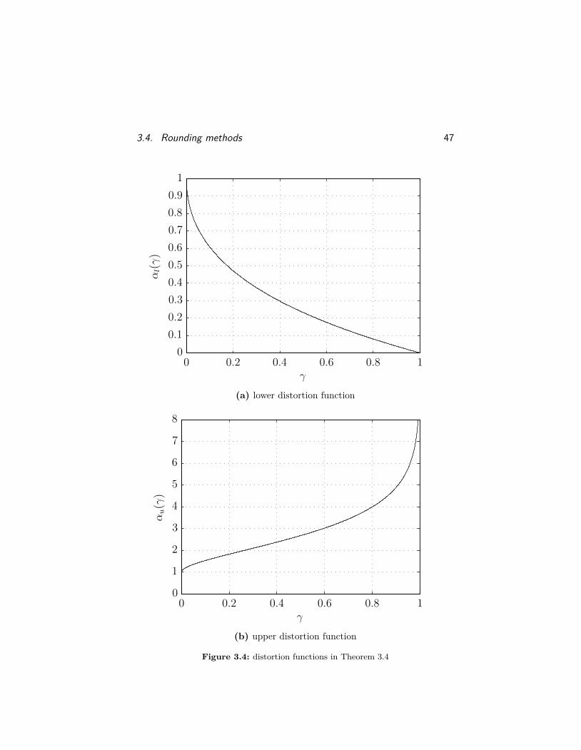
andWk is the kth branch of the LambertW function (see Remark 3.1).The distortion functions αl(γ) and αu(γ) are shown in Figure 3.4. Inparticular, if γ > 1 − (2m)−

2d , then there is positive probability that

X satisfies the distortion bounds αl(γ)bi ≤ Ai • X ≤ αu(γ)bi for alli = 1, . . . ,m.

3.4. Rounding methods 47αl(γ)

γ0 0.2 0.4 0.6 0.8 1

0

0.1

0.2

0.3

0.4

0.5

0.6

0.7

0.8

0.9

1

(a) lower distortion function

αu(γ)

γ0 0.2 0.4 0.6 0.8 1

0

1

2

3

4

5

6

7

8

(b) upper distortion function

Figure 3.4: distortion functions in Theorem 3.4


Proof. Suppose bi = 0. Then we have that

Ai • (V V T) = Ai •X = bi = 0,

so we can use Lemma A.3 to conclude that AiV = 0. This implies that

Ai • X = Ai • (V ZV T) = (AiV ) • (ZV T) = (0) • (ZV T) = 0.

Thus, X satisfies all homogeneous equality constraints exactly. In therest of the proof, we assume that the homogeneous equality constraintshave been discarded, so bi > 0 for i = 1, . . . ,m.

We are interested in bounding the probability that the distortionbounds are satisfied:


)= 1− prob

(m⋃i=1

(Ai • X < αl(γ)bi or Ai • X > αu(γ)bi

)).

Applying the union bound yields


)≥ 1−

m∑i=1

(prob

(Ai • X < αl(γ)bi

)+ prob

(Ai • X > αu(γ)bi

))= 1−

m∑i=1

prob(

(Ai • X)dbi

< αl(γ)d)

−m∑i=1

prob(

(Ai • X)dbi

> αu(γ)d).

(We can divide by bi without changing the direction of the inequalitydue to our assumption that the bi are all strictly positive.) Observethat we can write Ai • X and bi as

Ai • X = Ai • (V ZV T) = (V TAiV ) • Z,bi = Ai •X = Ai • (V V T) = tr(V TAiV ).


Using these observations, we can express our bound as


)≥ 1−

m∑i=1

prob(

((V TAiV ) • Z)dtr(V TAiV ) < αl(γ)d

)

−m∑i=1

prob(

((V TAiV ) • Z)dtr(V TAiV ) > αu(γ)d

).

Since V TAiV ∈ Sr is symmetric, it has an eigenvalue expansion

V TAiV =r∑j=1

λijqijqTij ,

where λi1, . . . , λir ∈ R are the eigenvalues of Ai, and qi1, . . . , qir ∈ Rr

form an orthonormal set of corresponding eigenvectors. Note thatV TAiV is positive semidefinite because Ai is positive semidefinite;therefore, the eigenvalues λij are nonnegative. Using this eigenvalueexpansion of V TAiV , the definition of Z, and the fact that the traceof a matrix is the sum of its eigenvalues, we have that

((V TAiV ) • Z)dtr(V TAiV ) = 1∑r

=1 λi

r∑j=1

λijqijqTij

• (1d

d∑k=1

zkzTk

) d=

r∑j=1

λij∑r=1 λi

d∑k=1

(qijzk)2

=r∑j=1

θij

d∑k=1

(qTijzk)2,

where we defineθij = λij∑r

=1 λi.

Observe that the θij are nonnegative, and satisfyr∑j=1

θij =r∑j=1

λij∑r=1 λi

= 1.

Because each zk is a standard normal random vector, and each qijis a unit vector, we have that each qT

ijzk is a standard normal random


variable. Additionally, because the zk are independent standard normalrandom vectors, and qi1, . . . , qir form an orthonormal set, we have that

E((qTij1zk1)(qT

ij2zk2)T)

= qTij1 E

(zk1z

Tk2

)qij2

= δk1k2qTij1qij2

= δk1k2δj1j2 .

Thus, qTij1zk1 and qT

ij2zk2 are uncorrelated unless j1 = j2 and k1 = k2.Since uncorrelated jointly normal random variables are independent,the qT

ijzk are independent standard normal random variables. This im-plies that

yij =d∑

k=1(qTijzk)2

is a chi-squared random variable with d degrees of freedom becauseit is the sum of the squares of d independent standard normal ran-dom variables. Moreover, the yij are independent because the qT

ijzk areindependent for j = 1, . . . , r and k = 1, . . . , d. Thus, we have that

((V TAiV ) • Z)dtr(V TAiV ) =

d∑j=1

θijyij ,

where the yij are independent chi-squared random variables with d

degrees of freedom, and θi1, . . . , θir are nonnegative scalars summingto 1 for all i = 1, . . . ,m. Therefore, we can apply Lemma C.2:

prob(

((V TAiV ) • Z)dtr(V TAiV ) < αl(γ)d

)

= prob

r∑j=1

θijyij < αl(γ)d

≤ (eαl(γ) exp(−αl(γ)))

d2

=(−eW0

(γ − 1e

)exp

(W0

(γ − 1e

))) d2

=(−e(γ − 1e

)) d2

= (1− γ)d2 ,


where we have made use of the fact that W0(y) exp(W0(y)) = y for ally ∈ (−1/e, 0) (see Remark 3.1). Note that we can apply the lemma eventhough the inequality inside the probability is strict since chi-squaredrandom variables are continuous, so the probability is the same whetherthe inequality is weak or strict. Similarly, Lemma C.1 tells us that

prob(

((V TAiV ) • Z)dtr(V TAiV ) > αu(γ)d

)

= prob

r∑j=1

θijyij > αu(γ)d

≤ (eαu(γ) exp(−αu(γ)))

d2

=(−eW−1

(γ − 1e

)exp

(W−1

(γ − 1e

))) d2

=(−e(γ − 1e

)) d2

= (1− γ)d2 .

Combining these results gives


)≥ 1− 2m(1− γ)

d2 .

Remark 3.1. A general discussion of the Lambert W function is givenby Corless, et al. [26]. For our purposes it suffices to know that the Wfunction satisfiesW (y) exp(W (y)) = y for all y ∈ (−1/e, 0). A sketch ofthe function that maps z to z exp(z) is shown in Figure 3.5. For everyy ∈ (−1/e, 0), there are exactly two values of z such that z exp(z) = y.The value of z such that z exp(z) = y and z ∈ (−1, 0) is given byW0(y); the value of z such that z exp(z) = y and z ∈ (−∞,−1) is givenby W−1(y).

52 Heuristics and Approximate Solutionszexp(z)

z−5 −4 −3 −2 −1 0

−0.4

−0.3

−0.2

−0.1

0

Figure 3.5: the function that maps z to z exp(z)

Part II

Applications

4Trust-Region Problems

A trust-region problem (4.1) is an optimization problem of the form

minimize xTP0x+ 2qT0 x+ r0

subject to aTi x ≤ bi, i = 1, . . . ,mxTPix+ 2qT

i x+ ri ≤ 0, i = 1, . . . , p‖x‖ = 1.

(4.1)

The optimization variable is x ∈ Rn, and the problem data area1, . . . , am ∈ Rn, b1, . . . , bm ∈ R, P0, . . . , Pp ∈ Sn, q0, . . . , qp ∈ Rn,and r0, . . . , rp ∈ R. We assume that P1, . . . , Pp are positive semidef-inite, so each quadratic inequality constraint represents an ellipsoid(or degenerate ellipsoid). However, note that the objective may not beconvex because we do not assume that P0 is positive semidefinite.

An important special case of (4.1) is the simple trust-region prob-lem, where m = p = 0. For example, the Levenberg-Marquardt algo-rithm for nonlinear programming solves an instance of the simple trust-region problem in each step of the algorithm. The simple trust-regionproblem is known to be much easier than the general trust-region prob-lem, and has been studied extensively [29, 37, 41, 44, 72, 73, 81, 90].Additionally, some algorithms for nonconvex quadratic programming,which is NP-hard in general, use the simple trust-region problem as a

54

4.1. SDP relaxation of a trust-region problem 55

subproblem [55, 101]. It is possible to show that there is no duality gapfor the simple trust-region problem [91]; however, a duality gap mayexist for the general trust-region problem (4.1).

Special cases of (4.1) with m = 0 and 0 < s ≤ 2 have also receivedconsiderable attention. For example, Peng and Yuan [77] considered theproblem of minimizing a quadratic function subject to two quadraticconstraints. Using properties of local minimizers [66], Martinez andSantos [67] presented an algorithm for minimizing a quadratic func-tion subject to two strictly convex quadratic constraints. Zhang [104]proposed an algorithm for the general quadratic case, and the two-dimensional trust-region problem was solved by Williamson [99]. Un-fortunately, a duality gap may exist for all of these problems.

In this chapter we describe approaches to solving trust-region prob-lems using semidefinite programming. The key step in the analysis istypically to demonstrate that the SDP relaxation has a rank-1 solutionfor certain special cases of (4.1).

4.1 SDP relaxation of a trust-region problem

Note that (4.1) is a quadratic optimization problem. The derivationsof the primal and dual SDP relaxations of such a problem are given inSection A.2.4. In particular, the primal SDP relaxation of (4.1) is

minimize Q0 •Xsubject to Li •X ≤ 0, i = 1, . . . ,m

Qi •X ≤ 0, i = 1, . . . , pFi •X = 1, i = 1, 2X � 0,

(4.2)

where the optimization variable is X ∈ Sn+1, and we define

Qi =[Pi qiqTi ri

], i = 0, . . . , p,

Li =[

0 (1/2)ai(1/2)aT

i −bi

], i = 1, . . . ,m,

F1 =[I 00 0

], and F2 =

[0 00 1

].

56 Trust-Region Problems

The corresponding dual relaxation is

maximize ν1 + ν2subject to

∑2i=1 νiFi −

∑mi=1 λiLi −

∑pi=1 µiQi + S = Q0

λ ≥ 0µ ≥ 0S � 0,

(4.3)

with variables λ ∈ Rm, µ ∈ Rp, ν ∈ R2, and S ∈ Sn+1. The comple-mentarity conditions for (4.2) and (4.3) are

λi(Li •X) = 0, i = 1, . . . ,mµi(Qi •X) = 0, i = 1, . . . , p

S •X = 0.

Since X and S are positive semidefinite, the last complementarity con-dition is equivalent to SX = 0.

We argue in Section A.2.4 that (4.2) is an exact relaxation if it hasa rank-1 solution. The following lemma gives sufficient conditions forthe existence of a rank-1 solution of (4.2).

Lemma 4.1. Suppose (4.2) and (4.3) are both solvable, and there isno duality gap. Let X and (λ, µ, ν, S) be solutions of (4.2) and (4.3),respectively. The boundary of the second-order cone is

bd(SOC) = {(x, t) ∈ Rn+1 | ‖x‖2 = t}.

If there exists a nonzero vector z ∈ range(X) ∩ bd(SOC) such that

(i) zTLiz ≤ 0 for i = 1, . . . ,m,

(ii) zTQiz ≤ 0 for i = 1, . . . , p,

(iii) λi(zTLiz) = 0 for i = 1, . . . ,m, and

(iv) µi(zTQiz) = 0 for i = 1, . . . , p,

then (4.2) is an exact relaxation of (4.1).

4.1. SDP relaxation of a trust-region problem 57

Proof. Since we assume z ∈ bd(SOC), we have that ‖z1:n‖ = zn+1,where z1:n = (z1, . . . , zn) is the vector consisting of the first n compo-nents of z. Because we also assume that z is nonzero, it must be thecase that zn+1 is nonzero, and hence that we can define the matrix

X = 1z2n+1

zzT.

We have that rank(X) = 1 since X is a positive multiple of a nonzerodyad. We will show that X is a solution of (4.2) by showing that it isfeasible, and satisfies the complementarity conditions. Since we assumethat zTLiz ≤ 0 for i = 1, . . . ,m, we have that

Li • X = zTLiz

z2n+1

≤ 0, i = 1, . . . ,m.

Similarly, the assumption that zTQiz ≤ 0 for i = 1, . . . , p implies that

Qi • X = zTQiz

z2n+1

≤ 0, i = 1, . . . , p.

Using the definitions of F1 and F2, we find that

F1 • (zzT) = zTF1z = ‖z1:n‖2 and F2 • (zzT) = zTF2z = z2n+1.

Therefore, we have that

F1 • X = ‖z1:n‖2

z2n+1

= 1 and F2 • X =z2n+1z2n+1

= 1.

Additionally, we have that X is positive semidefinite because it is apositive multiple of a dyad. Taken together, these results show that Xis feasible for (4.2).

Our assumptions that λi(zTLiz) = 0 and µi(zTQiz) = 0 imply that

λi(Li • X) = λi(zTLiz)z2n+1

= 0 and µi(Qi • X) = µi(zTQiz)z2n+1

= 0.

Since z ∈ range(X), there exists a vector z such that z = Xz. Wehave that SX = 0 because S and X are solutions of their respective


problems, and therefore satisfy complementary slackness. Combiningthese results, we find that

SX = 1z2n+1

SzzT = 1z2n+1

SXzzT = 0.

Thus, we have shown that X is feasible, and satisfies the complemen-tarity conditions. This implies that X is a solution of (4.2).

4.2 The simple trust-region problem

The simple trust-region problem (4.4) is a special case of (4.1) withm = p = 0:


subject to ‖x‖ = 1.(4.4)

SDP relaxation of the simple trust-region problem

The SDP relaxation of (4.4) is

minimize Q0 •Xsubject to Fi •X = 1, i = 1, 2

X � 0.

(4.5)

This problem has m = 2 equality constraints, so Theorem 2.1 guar-antees the existence of a rank-1 solution. Thus, this SDP relaxation isexact. In particular, if X = vvT ∈ Sn+1 is a rank-1 solution of (4.5),where v ∈ Rn+1, then x = vn+1(v1, . . . , vn) is a solution of (4.4).

4.3 Linear equality constraints

It turns out that adding linear equality constraints to (4.4) does notmake the problem more difficult – we can reduce such a problem to aninstance of (4.4). Consider the problem


subject to Ax = b

‖x‖ = 1,

4.3. Linear equality constraints 59

where we assume that A ∈ Rm×n is fat and full rank. (Note that ifA is not fat and full rank, then some of the equality constraints areeither redundant or inconsistent. We can use Gaussian elimination todetect inconsistent constraints, or to identify and remove redundantconstraints.) Let xmn = A†b denote the minimum-norm solution ofAx = b, where A† is the pseudoinverse of A. The problem is infeasibleif ‖xmn‖ > 1; if ‖xmn‖ = 1, then xmn is the solution of (4.4) becauseit is the only feasible point. (Note that the minimum-norm solutionof Ax = b is unique because we assume that A is fat and full rank.)Now consider the case when ‖xmn‖ < 1. We can write every solutionof Ax = b in the form x = xmn + z, where z ∈ null(A). We can thenreformulate (4.4) in terms of the variable z:

minimize zTP0z + 2(q0 + P0xmn)Tz + (xTmnP0xmn + 2qT

0 xmn + r0)subject to Az = 0

‖z‖ = (1− ‖xmn‖2)12 .

In this reformulation we have used the fact that the minimum-normsolution xmn is in the orthogonal complement of null(A), so that

‖xmn + z‖2 = ‖xmn‖2 + 2xTmnz + ‖z‖2 = ‖xmn‖2 + ‖z‖2.

Therefore, we can write the condition ‖x‖ = 1 as

‖z‖ = (1− ‖xmn‖2)12 .

We have that dim(null(A)) = m − n since we assume that A is fatand full rank. Let N ∈ Rn×(m−n) be a matrix whose columns forman orthonormal basis for null(A). Then every z ∈ null(A) can bewritten as z = (1 − ‖xmn‖2)

12Nw, where w ∈ Rm−n. Expressing our

optimization problem in terms of w gives a simple trust-region problem:

minimize wTPw + 2qTw + r

subject to ‖w‖ = 1,

where we define

P = (1− ‖xmn‖2)NTP0N

q = (1− ‖xmn‖2)12NT(P0xmn + q0)

r = xTmnP0xmn + 2qT

0 xmn + r0.


We obtain the constraint in our reformulated problem by noting that

‖w‖ = ‖Nw‖ = ‖(1− ‖xmn‖2)−12 z‖ = 1

because N has orthonormal columns, and ‖z‖ = (1− ‖xmn‖2)12 .

4.4 Linear inequality constraints

We have shown that a trust-region problem with linear equality con-straints can be reduced to an instance of (4.4). Now consider a trust-region problem with linear inequality constraints


subject to aTi x ≤ bi, i = 1, . . . ,m‖x‖ = 1.

(4.6)

4.4.1 Feasibility problems

First, we consider the feasibility problem associated with (4.6): that is,given vectors a1, . . . , am ∈ Rn and b ∈ Rm, we want to determine ifthere is a vector x ∈ Rn satisfying the constraints

aTi x ≤ bi, i = 1, . . . ,m,‖x‖ = 1.

(4.7)

We assume that a1, . . . , am are linearly independent. (If a1, . . . , am arelinearly dependent, then either there are variables that can be elimi-nated, or there are constraints that are either redundant or inconsistent;we can address these issues using Gaussian elimination.) Since we as-sume that a1, . . . , am are linearly independent, it must be the case thatthe system of equations

aTi x = bi, i = 1, . . . ,m

has a solution. Moreover, a system of equations and inequalities ob-tained by relaxing some of these equations to inequalities must alsohave a solution because every relaxation of a feasible problem is alsofeasible. First, we show that (4.7) is NP-hard in the general case.

Theorem 4.2. It is NP-hard to decide if (4.7) has a solution.

4.4. Linear inequality constraints 61

Proof. We will give a polynomial-time reduction to (4.7) from the par-tition problem, which is known to be NP-hard [36]. In the partitionproblem, we are given a set of integers {a1, . . . , aN}, and we want todetermine if there exists a subset S of {1, . . . , N} such that∑

i∈Sai =

∑i/∈S

ai.

Define the vector a = (a1, . . . , aN ) ∈ RN , and consider the followinginstance of (4.7):

±√N(a,−a)Tx ≤ 0

±(ej , ej)Tx ≤ ±1/√N, j = 1, . . . , N

(−ej , 0)Tx ≤ 0, j = 1, . . . , N(0,−ej)Tx ≤ 0, j = 1, . . . , N

‖x‖ = 1,

where x ∈ R2N . Note that this problem has m = 4N + 2 linear in-equality constraints. Let x = (u, v), where u, v ∈ RN . We can expressour instance of (4.7) in terms of u and v as

(√Na)Tu = (

√Na)Tv

uj + vj = 1/√N, j = 1, . . . , N

uj , vj ≥ 0, j = 1, . . . , N‖u‖2 + ‖v‖2 = 1.

If u and v satisfy the second and fourth of these conditions, then

N∑j=1

ujvj = 12

N∑j=1

((uj + vj)2 − (u2j + v2

j ))

= 12

N∑j=1

( 1√N

)2−

N∑j=1

u2j +

N∑j=1

v2j

= 1

2(1− (‖u‖2 + ‖v‖2)

)= 0.


Since uj , vj ≥ 0, this implies that ujvj = 0 for j = 1, . . . , N . Thus,there is a one-to-one correspondence between subsets S of {1, . . . , N},and vectors x = (u, v) satisfying the constraints

uj + vj = 1√N, uj , vj ≥ 0, and ‖u‖2 + ‖v‖2 = 1.

In particular, given a subset S of {1, . . . , N}, we set

uj =

1/√N j ∈ S,

0 otherwise,and vj =

1/√N j /∈ S,

0 otherwise.

Similarly, given vectors u and v satisfying the constraints, we take

S = {j ∈ {1, . . . , N} |uj = 1/√N}.

Intuitively, we can think of√Nu and

√Nv as the indicator vectors for

the set S and its complement, respectively. This implies that∑i∈S

ai = (√Na)Tu and

∑i/∈S

ai = (√Na)Tv.

Thus, we have∑i∈S ai =

∑i/∈S ai if and only if (

√Na)Tu = (

√Na)Tv.

This proves that the partition problem is equivalent to the given in-stance of (4.7), and hence that (4.7) is NP-hard.

Although Theorem 4.2 states that (4.7) is NP-hard in general, thefollowing theorem shows that we can solve (4.7) in polynomial timeunder an additional technical assumption.

Theorem 4.3. Suppose there exists an integer α < m such that |A| ≤ αfor every index set A ⊆ {1, . . . ,m} with the property that

{x ∈ Rn | ‖x‖ ≤ 1, aTi x = bi for i ∈ A} 6= ∅.

Then we can compute a solution of (4.7) in polynomial time.

Proof. Let x0 be a solution of

minimize ‖x‖2

subject to aTi x ≤ bi, i = 1, . . . ,m.


(We can solve this problem efficiently using standard algorithms.) If‖x0‖ > 1, then (4.7) is infeasible; if ‖x0‖ = 1, then x0 is a solution of(4.7). Thus, we can focus on the case when ‖x0‖ < 1. Choose an indexset A ⊆ {1, . . . ,m} with |A| > α, and let x1 be a solution of the convexquadratic program:

minimize ‖x‖2

subject to aTi x = bi, i ∈ AaTi x ≤ bi, i /∈ A.

Note that this problem is feasible because we assume that a1, . . . , amare linearly independent. Additionally, because |A| > α, we have that‖x1‖ > 1. Let

x(θ) = θx0 + (1− θ)x1.

For every θ ∈ [0, 1], the vector x(θ) satisfiesaTi x(θ) = θ(aT

i x0) + (1− θ)(aTi x1) ≤ θbi + (1− θ)bi = bi.

Note that the function f(θ) = ‖x(θ)‖ is continuous,f(0) = ‖x0‖ < 1, and f(1) = ‖x1‖ > 1.

Therefore, the intermediate-value theorem guarantees the existence ofa θ ∈ [0, 1] such that f(θ) = 1. We can find such a θ efficiently using,for example, bisection on θ. Then x(θ) is a solution of (4.7).

The proof of Theorem 4.3 easily generalizes to the case when thereare linear equality constraints.Theorem 4.4. Consider the feasibility problem

aTi x ≤ bi, i = 1, . . . ,mCx = d

‖x‖ = 1with variable x ∈ Rn, and problem data a1, . . . , am ∈ Rn, b ∈ Rm,C ∈ Rp×n, and d ∈ Rp. We can assume without loss of generality thatthe rows of the matrix

aT1...aTm

C


are linearly independent. Suppose there exists an integer α < m suchthat |A| ≤ α for every index set A ⊆ {1, . . . ,m} with the property that

{x ∈ Rn | ‖x‖ ≤ 1, Cx = d, aTi x = bi for i ∈ A} 6= ∅.

Then we can compute a solution of the feasibility problem above inpolynomial time.

4.4.2 SDP-SOCP relaxation

Adding redundant (also called valid) constraints to an optimizationproblem does not change the optimal set or optimal value of the prob-lem. Intuitively, the Lagrangian relaxation constructs a lower bound onthe optimal value of an optimization problem using linear combinationsof the constraints. Therefore, adding redundant constraints may resultin tighter relaxations (that is, smaller duality gaps) because there aremore constraints that can be used to construct the lower bound. Per-haps the most famous examples of valid inequalities are Gomory cuts,which were introduced by Gomory [42, 43], and used in practical algo-rithms by Cornuéjols [27, 28]. Adding valid inequalities to (4.6) givesthe problem


subject to ‖(bi − aTi x)x‖ ≤ bi − aT

i x, i = 1, . . . ,m(bi − aT

i x)(bj − aTj x) ≥ 0, 1 ≤ i < j ≤ m

‖x‖ = 1.

Due to the constraint ‖x‖ = 1, we have that

‖(bi − aTi x)x‖ = |bi − aT

i x|‖x‖ = |bi − aTi x|.

Thus, the constraint ‖(bi − aTi x)x‖ = |bi − aT

i x| ≤ bi − aTi x is equiv-

alent to the inequality bi − aTi x ≥ 0, which can also be written as

aTi x ≤ bi. However, the more complicated formulation of these con-

straints gives a tighter relaxation. Similarly, because aTi x ≤ bi, the

constraints (bi − aTi x)(bj − aT

j x) ≥ 0 are redundant; nonetheless, weinclude these constraints because they result in a tighter relaxation.


We can express the problem with the added valid constraints as

minimize[P0 q0qT

0 r0

]•

[x1

] [x

1

]T

subject to [x1

] [x

1

]T[−ai

bi

]∈ SOC, i = 1, . . . ,m

[−aibi

]T[x

1

] [x

1

]T[−aj

bj

]≥ 0, 1 ≤ i < j ≤ m

[I 00 0

]•

[x1

] [x

1

]T = 1.

Since the set of dyads is equal to the set of rank-1, positive-semidefinitematrices, we can rewrite this problem as

minimize C •Xsubject to Fi •X = 1, i = 1, 2

cTi Xcj ≥ 0, 1 ≤ i < j ≤ mXci ∈ SOC, i = 1, . . . ,mX � 0rank(X) = 1,

where we define the matrices F1, F2 ∈ Sn+1, and the vectorsc1, . . . , cm ∈ Rn+1 such that

F1 =[I 00 0

], F2 =

[0 00 1

], and ci =

[−aibi

].

Ignoring the rank constraint gives an SDP-SOCP relaxation of (4.6):


Aij •X ≥ 0, 1 ≤ i < j ≤ mXci ∈ SOC, i = 1, . . . ,mX � 0,

(4.8)

where Aij ∈ Sn+1 is the symmetric part of cicTj :

Aij = 12(cicT

j + cjcTi ).


If we can show that (4.8) has a rank-1 solution, then (4.8) is an exactrelaxation of (4.6): that is, (4.8) and (4.6) have the same optimal value,and X = vvT is a rank-1 solution of (4.8) if and only if x = vn+1v1:n isa solution of (4.6). Our analysis will use the dual of (4.8):

maximize λ1 + λ2subject to

∑2i=1 λiFi +

∑m−1i=1

∑mj=i+1 µijAij

+(1/2)∑mi=1(νicT

i + ciνTi ) + S = C

µij ≥ 0, 1 ≤ i < j ≤ mνi ∈ SOC, i = 1, . . . ,mS � 0,

(4.9)

where the variables are λi, µij ∈ R, νi ∈ Rn+1, and S ∈ Sn. Thecomplementarity conditions for (4.8) and (4.9) are

µij(Aij •X) = 0, 1 ≤ i < j ≤ mνTi Xci = 0, i = 1, . . . ,mS •X = 0.

Since X and S are positive semidefinite, the last complementarity con-dition is equivalent to SX = 0. The following lemma gives sufficientconditions for (4.8) to be an exact relaxation of (4.6).

Lemma 4.5. Suppose (4.8) and (4.9) are both solvable, and there isno duality gap. Let X and (λ, µ, ν, S) be solutions of (4.8) and (4.9),respectively. If there exists a nonzero vector z ∈ range(X)∩bd(SOC)such that

(i) cTi z ≥ 0 for i = 1, . . . ,m,

(ii) µij(cTi z)(cT

j z) = 0 for 1 ≤ i < j ≤ m, and

(iii) (cTi z)(νT

i z) = 0 for i = 1, . . . ,m,


Proof. Since z is on the boundary of SOC, we have that ‖z1:n‖ = zn+1.Because we also assume that z is nonzero, zn+1 must be nonzero, sowe can define the matrix

X = 1z2n+1

zzT.


We have that rank(X) = 1 since X is a positive multiple of a dyad.We will show that X is a solution of (4.8) by showing that it is feasible,and satisfies the complementarity conditions. The definitions of F1 andF2 imply that

F1 • X = zTF1z

z2n+1

= ‖z1:n‖2

z2n+1

= 1

F2 • X = zTF2z

z2n+1

=z2n+1z2n+1

= 1.

We have that X is positive semidefinite because it is a positive multipleof a dyad. The assumption that cT

i z ≥ 0 for i = 1, . . . ,m guarantees

Aij • X =(cTi z)(cT

j z)z2n+1

≥ 0.

Similarly, because cTi z ≥ 0, z ∈ SOC, and SOC is closed under non-

negative scaling, we have that

Xci = cTi z

z2n+1

z ∈ SOC.

We have now shown that X is feasible for (4.8).Our assumption that µij(cT

i z)(cTj z) = 0 implies that

µij(Aij • X) =µij(cT

i z)(cTj z)

z2n+1

= 0

for 1 ≤ i < j ≤ m. Similarly, the assumption that (cTi z)(νT

i z) = 0guarantees that

νTi Xci = (cT

i z)(νTi z)

z2n+1

= 0

for i = 1, . . . ,m. Since z ∈ range(X), there exists a vector z such thatz = Xz. We have that SX = 0 because S and X are solutions of theirrespective problems, and therefore satisfy complementary slackness.Combining these results, we find that

SX = 1z2n+1

SzzT = 1z2n+1

SXzzT = 0.

Thus, we have shown that X is feasible, and satisfies the complemen-tarity conditions. This implies that X is a solution of (4.8).


At most one inactive inequality constraint

Consider the optimization problem


subject to aTi x ≤ bi, i = 1, . . . ,m

(bi − aTi x)(bj − aT

j x) = 0, 1 ≤ i < j ≤ m‖x‖ = 1.

(4.10)

Recall that an inequality constraint is said to be active or binding if itholds with equality. Thus, (4.10) requires that at most one inequalityconstraint is inactive because the constraint (bi−aT

i x)(bj−aTj x) = 0 is

satisfied if and only if aTi x = bi or aT

j x = bj . The SDP-SOCP relaxationof (4.10) is


Aij •X = 0, 1 ≤ i < j ≤ mXci ∈ SOC, i = 1, . . . ,mX � 0.

(4.11)

The corresponding dual relaxation is

maximize λ1 + λ2subject to

∑2i=1 λiFi +

∑m−1i=1

∑mj=i+1 µijAij

+(1/2)∑mi=1(νicT

i + ciνTi ) + S = C

νi ∈ SOC, i = 1, . . . ,mS � 0.

(4.12)

The complementarity conditions for these relaxations are

νTi Xci = 0, i = 1, . . . ,mS •X = 0.

Since S and X are positive semidefinite, the last complementarity con-dition is equivalent to SX = 0. We will show that if there is no dualitygap between (4.11) and (4.12), then (4.11) is an exact relaxation of(4.10). Our analysis will use the following lemma, which gives suffi-cient conditions for the SDP-SOCP relaxation to be exact.


Lemma 4.6. Suppose there is no duality gap between (4.11) and (4.12).If there exists a nonzero vector z ∈ range(X) ∩ bd(SOC) such that

(i) cTi z ≥ 0 for i = 1, . . . ,m,

(ii) (cTi z)(cT

j z) = 0 for 1 ≤ i < j ≤ m, and

(iii) (cTi z)(νT

i z) = 0 for i = 1, . . . ,m,


Proof. Let X be a solution of (4.11), and (λ, µ, ν, S) be a solutionof (4.12). In addition to satisfying the constraints of their respectiveproblems, these solutions must satisfy the complementarity conditions

SX = 0 and νTi Xci = 0, i = 1, . . . ,m.

Suppose z satisfies the hypotheses above. Because z ∈ bd(SOC), wehave that ‖z1:n‖ = zn+1. Since, in addition, z is assumed to be nonzero,this implies that zn+1 is nonzero. Therefore, we can define the matrix

X = 1z2n+1

zzT.

The definitions of F1 and F2, imply that

F1 • X = zTF1z

z2n+1

= ‖z1:n‖2

z2n+1

= 1,

F2 • X = zTF2z

z2n+1

=z2n+1z2n+1

= 1.

Our assumption that (cTi z)(cT

j z) = 0 for 1 ≤ i < j ≤ m implies that

Aij • X =(cTi z)(cT

j z)z2n+1

= 0.

Since z ∈ SOC, cTi z ≥ 0, and SOC is closed under nonnegative scaling,

we have thatXci = cT

i z

z2n+1

z ∈ SOC.

Note that X is positive semidefinite because it is a positive multiple ofa dyad. We have now shown that X satisfies the constraints of (4.11);


it remains to check that X satisfies the complementarity conditions.Our assumption that (cT

i z)(νTi z) = 0 implies that

νTi Xci = (cT

i z)(νTi z)

z2n+1

= 0.

Finally, because z ∈ range(X), we have that z = Xz for some vectorz, and hence that

SX = 1z2n+1

SzzT = 1z2n+1

SXzzT = 0,

where we use the fact that SX = 0. Having shown that X is feasible,and satisfies the complementarity conditions, we can conclude that Xis optimal. Moreover, it is clear that rank(X) = 1 because X is a scalarmultiple of a dyad.

We are now prepared to show that (4.11) is an exact relaxation of(4.10). We will rely heavily on Lemma 4.6.

Theorem 4.7. If there is no duality gap between (4.11) and (4.12),then (4.11) has a rank-1 solution, which implies that (4.11) is an exactrelaxation of (4.10).

Proof. Let X be a solution of (4.11), and (λ, µ, ν, S) be a solution of(4.12). We will show how to construct a rank-1 solution of (4.11). Thereare three cases to consider.

(1) First, suppose Xc1 = · · · = Xcm = 0. Let r = rank(X), anduse Lemma A.10 to find vectors z1, . . . , zr such that

X =r∑j=1

zizTi and zT

j (F1 − F2)zj = (F1 − F2) •Xr

= 0,

where (F1−F2)•X = (F1 •X)− (F2 •X) = 1−1 = 0 because Xis feasible for (4.11). Then we have that zj ∈ bd(SOC) because

zT(F1 − F2)zj = ‖(zj)1:n‖2 − (zj)2n+1 = 0.

Note that z1, . . . , zr must be linearly independent since they forma dyadic decomposition of the rank-r matrix X. This implies that


the zj are all nonzero. Moreover, the fact that

Xci =r∑j=1

(cTi zj)zj = 0

implies that cTi zj = 0 for all i and j. We have that zj ∈ range(X)

because the zj form a dyadic decomposition for X. To summa-rize, we have shown that the zj are nonzero vectors contained inrange(X) ∩ bd(SOC) such that cT

i zj = 0 for all i and j. Thisimplies that each of the zj satisfies the hypotheses of Lemma 4.6,and hence that (4.11) is an exact relaxation of (4.10).

(2) Next, consider the case when at least one of the Xci is anonzero vector on the boundary of SOC. We can assume withoutloss of generality that Xc1 is such a vector. Let z = Xc1. We havethat cT

1 z = cT1Xc1 ≥ 0 because X � 0; we also have that

cTj z = cT

1Xcj = A1j •X = 0

for j = 2, . . . ,m because X is feasible for (4.11). This implies that(cTi z)(cT

j z) = 0 for 1 ≤ i < j ≤ m. Complementarity requires thatνT

1 Xc1 = 0, and hence that (cT1 z)(νT

1 z) = (cT1 z)(νT

1 Xc1) = 0.Having already shown that cT

j z = 0, we can conclude that(cTj z)(νT

j z) = 0 for j = 2, . . . ,m. Since X and S are solutionsof their respective problems, they satisfy the complementary-slackness condition SX = 0; this implies that Sz = SXc1 = 0.We have now shown that z satisfies the hypotheses of Lemma 4.6,and hence that (4.11) is an exact relaxation of (4.10).

(3) Finally, consider the case when at least one of the Xci iscontained in the interior of SOC. Without loss of generality, wecan assume that Xc1 is in the interior of SOC. Define the matrixP ∈ Sn+1 such that

P =m∑i=1

(X12 ci)(X

12 ci)†.

In our expression for P , we take the pseudoinverse of columnvectors; recall that the pseudoinverse of a column vector q is


given by

q† =

(1/‖q‖2)qT q 6= 0,0 q = 0.

Note that Xc1 is nonzero because it is in the interior of SOC.Thus, we have that

P = 1cT

1Xc1(X

12 c1)(X

12 c1)T

+m∑i=2

(1/(cTi Xci))(X

12 ci)(X

12 ci)T X

12 ci 6= 0,

0 X12 ci = 0.

Define the matrix Z ∈ Sn+1 such that

Z = X12 (I − P )X

12

= X − 1cT

1Xc1(Xc1)(Xc1)T

−m∑i=2

(1/(cTi Xci))(Xci)(Xci)T X

12 ci 6= 0,

0 X12 ci = 0.

Because Xci ∈ SOC, we have that

(F1 − F2) • ((Xci)(Xci)T) = (Xci)TF1(Xci)− (Xci)TF2(Xci)= ‖(Xci)1:n‖2 − (Xci)2

n+1

≤ 0.

Moreover, this inequality is strict for i = 1 because Xc1 is in theinterior of SOC. Combined with the fact that (F1 − F2) •X = 0since X is feasible, this allows us to conclude that

(F1 − F2) • Z

= (F1 − F2) •X − (F1 − F2) • ((Xc1)(Xc1)T)cT

1Xc1

−

((F1 − F2) • ((Xci)(Xci)T))/(cTi Xci) X

12 ci 6= 0,

0 X12 ci = 0.

> 0.


This implies that Z is nonzero, and hence that s = rank(Z) > 0.Use Lemma A.10 to find vectors u1, . . . , us such that

Z =s∑j=1

ujuTj and uT

j (F1 − F2)uj = (F1 − F2) • Zs

> 0.

Then our choice of u1, . . . , us implies that

uTj (F1 − F2)uj = ‖(uj)1:n‖2 − (uj)2

n+1 > 0,

so that uj /∈ SOC. We will use u1 to construct a vector z satis-fying the hypotheses of Lemma 4.6; however, this choice is some-what arbitrary: any of the uj would serve as well. Because Xc1is in the interior of SOC, and u1 is not contained in SOC, thereexists θ ∈ (0, 1) such that

z = θXc1 + (1− θ)u1

is on the boundary of SOC. Suppose z is equal to zero. Then wehave that u1 = −(θ/(1− θ))Xc1, and hence that

uT1 (F1 − F2)u1 =

(θ

1− θ

)2(Xc1)T(F1 − F2)(Xc1)

=(

θ

1− θ

)2(‖(Xc1)1:n‖2 − (Xc1)2

n+1)

< 0,

where we use the fact that ‖(Xc1)1:n‖2 < (Xc1)2n+1 because

Xc1 is in the interior of SOC. This contradicts the fact thatu1 was chosen such that uT

1 (F1 − F2)u1 > 0, and thereby provesthat z must be nonzero. We have that u1, . . . , us form a basisfor range(Z) ⊂ range(X

12 ) = range(X). Thus, we have that

u1 ∈ range(X). Since we also have that Xc1 ∈ range(X), wecan conclude that

z = θXc1 + (1− θ)u1 ∈ range(X).

For a column vector q, we think of qq† as the projection onto q.We have that X

12 ci and X

12 cj are orthogonal because

(X12 ci)T(X

12 cj) = cT

i Xcj = Aij •X = 0.


This implies that P is the orthogonal projection onto the subspacespan(X

12 c1, . . . , X

12 cm). Therefore, we have that PX

12 ci = X

12 ci,

and hence that

Zci = X12 (I − P )X

12 ci

= X12 (X

12 c1 − PX

12 ci)

= X12 (X

12 ci −X

12 ci)

= 0.

Note that u1, . . . , us are linearly independent because they forma dyadic expansion of the rank-s matrix Z. Then the fact that

Zci =s∑j=1

(cTi uj)uj = 0

implies that cTi uj = 0 for all i and j. Since X � 0, we have that

cT1Xc1 ≥ 0. Combining these results, we find that

cT1 z = θcT

1Xc1 + (1− θ)cT1 u1 = θcT

1Xc1 ≥ 0.

Similarly, we have that

cTj z = θcT

1Xcj + (1− θ)cTj u1 = θ(A1j •X) = 0

for j = 2, . . . ,m. Taken together, these results imply that cTi z ≥ 0

for i = 1, . . . ,m, (cTi z)(cT

j z) = 0 for 1 ≤ i < j ≤ m, and(cTi z)(νT

i z) = 0 for i = 2, . . . ,m. Since Xc1 is in the interiorof SOC, complementarity implies that ν1 = 0, and hence that(cT

1 z)(νT1 z) = 0. We have now shown that z satisfies the hypothe-

ses of Lemma 4.6, which proves that (4.11) is an exact relaxationof (4.10).

The cases above are collectively exhaustive, and therefore suffice toshow that (4.11) is an exact relaxation of (4.10).

Non-intersecting pairs of linear constraints

Now we consider an instance of (4.6) with two non-intersecting lin-ear constraints. When we say the linear constraints of (4.6) do not


intersect, we mean that there is no vector x such that ‖x‖ ≤ 1 andaTi x = bi for i = 1, 2. The results in this section are due to Burer and

Anstreicher [13], and Burer and Yang [19].

Theorem 4.8. Suppose m = 2, (4.8) and (4.9) are both solvable, andthere is no duality gap. If

{x ∈ Rn | aT1 x = b1, a

T2 x = b2, ‖x‖ ≤ 1} = ∅,


Proof. Let X be a solution of (4.8), and (λ, µ, ν, S) be a solution of(4.9). If A12 •X = 0, then we can find a rank-1 solution of (4.8) usingthe construction in the proof of Theorem 4.7. Thus, we only need toconsider the case when A12 • X > 0. In this case complementarityimplies that µ12 = 0, and hence that we can use Lemma 4.5 to deducethat there exists a rank-1 solution of (4.8) if we can find a nonzeroz ∈ range(X) ∩ bd(SOC) such that

cT1 z, c

T2 z ≥ 0 and (cT

1 z)(νT1 z) = (cT

2 z)(νT2 z) = 0.

Because we are considering the case when cT1Xc2 = A12 • X > 0, we

have that Xc1 and Xc2 are nonzero. We divide the analysis into cases.

(1) First, consider the case when Xc1 and Xc2 are linearly de-pendent. Since Xc1 and Xc2 are nonzero, this implies that thereexists a nonzero scalar α such that Xc1 = αXc2. Moreover, αmust be positive because Xc1, Xc2 ∈ SOC.

(1)(a) Suppose Xc1 ∈ bd(SOC). Then we claim that the vectorz = Xc1 = αXc2 has the desired properties. BecauseX is positivesemidefinite, we have that cT

1 z = cT1Xc1 ≥ 0. Similarly, we have

that cT2 z = α(cT

2Xc2) ≥ 0 since X � 0 and α > 0. Because Xand ν1 are optimal, they satisfy the complementarity conditionνT

1 Xc1 = 0. Thus, z satisfies

νT1 z = νT

1 Xc1 = 0 and νT2 z = α(νT

2 Xc2) = 0.

This completes the proof that z satisfies the hypotheses ofLemma 4.5, and hence that (4.8) is an exact relaxation of (4.6).


(1)(b) Next, suppose Xc1 ∈ int(SOC). Then we also have thatXc2 = (1/α)Xc1 ∈ int(SOC), and hence that ν1 = ν2 = 0 dueto complementarity. The orthogonal projection onto the subspacespan(X

12 c1) = span(X

12 c2) is represented by the matrix

P = (X12 c1)((X

12 c1)T(X

12 c1))−1(X

12 c1)T

= 1cT

1Xc1(X

12 c1)(X

12 c1)T.

Define the matrix

Z = X12 (I − P )X

12 = X − 1

cT1Xc1

(Xc1)(Xc1)T.

Since Xc1 ∈ int(SOC), we have that

(F1 − F2) • ((Xc1)(Xc1)T) = (Xc1)T(F1 − F2)(Xc1)= ‖(Xc1)1:n‖2 − (Xc1)2

n+1

< 0.

Combined with the fact that (F1 − F2) • X = 0 because X isfeasible for (4.8), this allows us to conclude that

(F1 − F2) • Z = (F1 − F2) •X

− 1cT

1Xc1(F1 − F2) • ((Xc1)(Xc1)T)

> 0.

This implies that Z is nonzero. Let s = rank(Z) > 0, and useLemma A.10 to find z1, . . . , zs such that

Z =s∑i=1

zizTi and zT

i (F1 − F2)zi = (F1 − F2) • Zs

> 0.

We have that zi /∈ SOC because

zTi (F1 − F2)zi = ‖(zi)1:n‖2 − (zi)2

n+1 > 0.

Since Xc1 ∈ int(SOC) and zi /∈ SOC, there exists θ ∈ (0, 1)such that

z = θXc1 + (1− θ)z1 ∈ bd(SOC).


Suppose z = 0. Then we have that

z1 = − θ

1− θXc1,

and hence that

zT1 (F1 − F2)z1 =

(θ

1− θ

)2(Xc1)T(F1 − F2)(Xc1) < 0.

This contradicts our choice of z1, and thereby proves that z isnonzero. We have that PX

12 ci = X

12 ci because P is the projection

onto span(X12 c1) = span(X

12 c2). This implies that

Zci = X12 (I − P )X

12 ci

= X12 (X

12 ci − PX

12 ci)

= X12 (X

12 ci −X

12 ci)

= 0.

Therefore, we have that

Zci =s∑j=1

(cTi zj)zj = 0,

and hence that cTi zj = 0 because z1, . . . , zs are linearly indepen-

dent because they form a dyadic expansion of the rank-s matrixZ. Since X is positive semidefinite, we have that cT

i Xci ≥ 0 fori = 1, 2. Combined with the facts that cT

i zj = 0 and α > 0, thisallows us to conclude that

cT1 z = θ(cT

1Xc1) + (1− θ)(cT1 z1) ≥ 0,

cT2 z = αθ(cT

2Xc2) + (1− θ)(cT2 z1) ≥ 0.

This completes the proof that z satisfies the hypotheses ofLemma 4.5, and hence that (4.8) is an exact relaxation of (4.6).

(2) Now consider the case when Xc1 and Xc2 are linearly inde-pendent.

(2)(a) Suppose one of Xc1 and Xc2 is on the boundary of SOC,and the other is in the interior of SOC. Without loss of gen-erality, assume that Xc1 is on the boundary of SOC, and Xc2


is in the interior of SOC. We claim that z = Xc1 satisfies thehypotheses of Lemma 4.5. We have already shown that Xc1 isnonzero. It is clear that Xc1 ∈ range(X), and we assume thatXc1 ∈ bd(SOC). Since X � 0, we have that cT

1 z = cT1Xc1 ≥ 0.

Similarly, because X is feasible, we find that

cT2 z = cT

1Xc2 = A12 •X ≥ 0.

Since X and ν1 satisfy complementarity, we have that

νT1 z = νT

1 Xc1 = 0.

Because Xc2 ∈ int(SOC), we have that ν2 = 0, and hence thatνT

2 z = 0. This completes the proof that z satisfies the hypothesesof Lemma 4.5.(2)(b) Now consider the case when Xc1, Xc2 ∈ int(SOC). Let Pbe the projection onto span(X

12 c1, X

12 c2), and define the matrix

Z = X12 (I − P )X

12 .

(2)(b)(i) Suppose (F1 − F2) • Z ≥ 0. Use Lemma A.10 to findz1, . . . , zs such that

Z =s∑i=1

zizTi and zT

i (F1 − F2)zi = (F1 − F2) • Zs

≥ 0.

Because P is the projection onto span(X12 c1, X

12 c2), we have

that PX12 ci = X

12 ci, and hence that

Zci =s∑j=1

(cTi zj)zj = X

12 (I − P )X

12 ci = 0

for i = 1, 2. Since z1, . . . , zs are linearly independent, this impliesthat cT

i zj = 0 for i = 1, 2 and j = 1, . . . , s. Because z1 is nonzeroand contained in SOC, we have that

x = 1(z1)n+1

(z1)1:n

satisfies ‖x‖ ≤ 1. Recall that we defined ci = (−ai, bi). Thus, wehave that

cTi z1 = bi(z1)n+1 − aT

i (z1)1:n = 0,


and hence that

aTi x = aT

i (z1)1:n(z1)n+1

= bi.

Combining these observations, we see that we have found a vectorx such that aT

1 x = b1, aT2 x = b2, and ‖x‖ ≤ 1. This violates the

non-intersection assumption, so this case cannot happen.(2)(b)(ii) Now consider the case when (F1 − F2) • Z < 0. UseLemma A.10 to find z1, . . . , zs such that Z =

∑si=1 ziz

Ti , and

zTi (F1 −F2)zi = ((F1 −F2) •Z)/s, where s = rank(Z). Then wehave that Xc2 ∈ int(SOC), and z1 /∈ SOC, and we can use theconstruction in (1)(b) to find a rank-1 solution of the SDP-SOCPrelaxation.

(2)(c) Finally, consider the case when Xc1, Xc2 ∈ bd(SOC).Let P be the projection onto span(X

12 c1, X

12 c2), and define the

matrix Z = X12 (I − P )X

12 . Since X is feasible, it satisfies the

constraintcT

1Xc2 = (X12 c1)T(X

12 c2) = 0.

Thus, we have that X12 c1 and X

12 c2 are orthogonal, which implies

that the projection matrix P is given by

P =2∑i=1

(X12 ci)(X

12 ci)†

=2∑i=1

1cTi Xci

(X12 ci)(X

12 ci)T.

Using this expression for P , we find that

Z = X12 (I − P )X

12

= X −X12PX

12

= X −X12

( 2∑i=1

1cTi Xci

(X12 ci)(X

12 ci)T

)X

12

= X −2∑i=1

1cTi Xci

(Xci)(Xci)T.


Because Xc1 and Xc2 are on the boundary of the second-ordercone, we have that

(Xci)T(F1 − F2)(Xci) = ‖(Xci)1:n‖2 − (Xci)2n+1 = 0

for i = 1, 2. Additionally, we have that (F1−F2) •X = 0 since Xis feasible. Combining these results, we find that

(F1 − F2) • Z = (F1 − F2) •(X −

2∑i=1

1cTi Xci

(Xci)(Xci)T)

= (F1 − F2) •X −2∑i=1

(Xci)T(F1 − F2)(Xci)cTi Xci

= 0.

Thus, we have that (F1−F2)•Z = 0, and we can use the construc-tion in (2)(b)(i) to show that the non-intersection assumption isviolated. Therefore, this case cannot happen.

Burer and Anstreicher [13] give an example showing that the SDPrelaxation of an instance of (4.6) with m = 2 may not be exact if thelinear constraints intersect inside the unit ball.

Non-intersecting sets of linear constraints

Burer and Yang [19] extended Theorem 4.8 to the case of an arbitrarynumber of linear constraints such that no two constraints intersectinside the unit ball.

Theorem 4.9. Suppose (4.8) and (4.9) are both solvable, and there isno duality gap. If

{x ∈ Rn | aTi x = bi, a

Tj x = bj , ‖x‖ ≤ 1} = ∅

for all distinct i and j in {1, . . . ,m}, then (4.8) is an exact relaxationof (4.6).

Bienstock and Michalka [8] showed that (4.6) can be solved effi-ciently if the linear constraints satisfy the non-intersection conditiongiven in the following theorem.

4.5. Ellipsoidal quadratic inequality constraints 81

Theorem 4.10. The problem (4.6) can be solved in polynomial time ifthere exists a positive integer k > 1 with the property that

{x ∈ Rn | ‖x‖ ≤ 1, aTi x ≤ bi for all i ∈ I} = ∅

for all index sets I ⊂ {1, . . . ,m} such that |I| = k.

4.5 Ellipsoidal quadratic inequality constraints

Consider an instance of (4.1) with m = 0:


subject to xTPix+ 2qTi x+ ri ≤ 0, i = 1, . . . , p

‖x‖ = 1.

(4.13)

When there are no linear inequality constraints, (4.2) simplifies to

minimize Q0 •Xsubject to Qi •X ≤ 0, i = 1, . . . , p

Fi •X = 1, i = 1, 2X � 0.

(4.14)

Similarly, (4.3) simplifies to

minimize ν1 + ν2subject to

∑2i=1 νiFi −

∑pi=1 µiQi + S = Q0

µ ≥ 0S � 0.

(4.15)

4.5.1 Inactive quadratic constraints

The following result was given by Ye and Zhang [102].

Theorem 4.11. If p = 1, and there exists a solution X of (4.14)such that the quadratic inequality constraint is inactive at X (thatis, Q1 •X < 0)), then (4.14) is an exact relaxation of (4.13).

Proof. Suppose p = 1, X is a solution of (4.14) such that Q1 •X < 0,and (µ, ν, S) is a solution of (4.15). The fact that Q1 •X < 0 implies


that X is nonzero, and hence that r = rank(X) > 0. Use Lemma A.10to find z1, . . . , zr ∈ Rn such that

X =r∑i=1

zizTi and zT

i (F1 − F2)zi = (F1 − F2) •Xr

= 0,

where (F1−F2) •X = 0 because X is feasible for (4.14). We have that

Q1 •X = Q1 •(

r∑i=1

zizTi

)=

r∑i=1

zTi Q1zi < 0,

which implies that zTi Q1zi < 0 for some i. Without loss of generality,

assume that zT1 Q1z1 < 0. We claim that

z = sign((z1)n+1)z1

satisfies the hypotheses of Lemma 4.1. We have that z ∈ range(X)because z1, . . . , zr form a basis for range(X). We chose z1 such that

zT1 (F1 − F2)z1 = ‖(z1)1:n‖2 − (z1)2

n+1 = 0,

which implies that z is on the boundary of SOC. Since we have thatzTQ1z = zT

1 Q1z1 < 0, the vector z is nonzero, and zTQ1z ≤ 0. Com-plementarity requires that µ1 = 0 because Q1 •X < 0, and hence thatµ1(zTQ1z) = 0. We have now checked that z satisfies all of the hy-potheses of Lemma 4.1. Thus, we can conclude that (4.14) is an exactrelaxation of (4.13).

Burer and Anstreicher [13] showed that (4.14) may not be an exactrelaxation if there does not exist a solution for which the quadraticinequality constraint is strictly satisfied.

Convex quadratic constraints

We can also show that (4.14) is an exact relaxation of (4.13) whenQ1, . . . , Qp are positive semidefinite. The characterization of positive-semidefinite block matrices given in Corollary A.12 tells us that theblock matrix Qi is positive semidefinite if and only if Pi is positivesemidefinite, qi ∈ range(Pi), and ri − qT

i P†i qi ≥ 0. Thus, requiring

that Q1, . . . , Qp be positive semidefinite is a stronger condition thanrequiring that (4.13) be a convex optimization problem.

4.5. Ellipsoidal quadratic inequality constraints 83

Theorem 4.12. Suppose Q1, . . . , Qp � 0. If (4.14) and (4.15) are bothsolvable, and there is no duality gap, then (4.14) is an exact relaxationof (4.13).

Proof. Suppose Q1, . . . , Qp are positive semidefinite, X is a solution of(4.14), and (µ, ν, S) is a solution of (4.15). Since X and Qi are positivesemidefinite, Lemma A.1 tells us that Qi • X ≥ 0. We also have thatQi•X ≤ 0 for i = 1, . . . , p because X is feasible for (4.14). Therefore, itmust be the case that Qi •X = 0 for i = 1, . . . , p. Since Xn+1,n+1 = 1,we have that r = rank(X) > 0. Then we can use Lemma A.10 to findz1, . . . , zr ∈ Rn such that

X =r∑i=1

zizTi and zT

i (F1 − F2)zi = (F1 − F2) •Xr

= 0,

where (F1−F2)•X = 0 because X is feasible for (4.14). We claim that

z = sign((z1)n+1)z1

satisfies the hypotheses of Lemma 4.1. We have that z is nonzero andcontained in range(X) because z1, . . . , zr form a basis for range(X).Additionally, since

zT1 (F1 − F2)z1 = zT(F1 − F2)z = ‖z1:n‖2 − z2

n+1 = 0,

and zn+1 ≥ 0, we have that z is on the boundary of SOC. BecauseQi •X = 0 for i = 1, . . . , p, we have that

Qi •X = Qi •

r∑j=1

zjzTj

=r∑j=1

zTj Qizj = 0.

Since Qi � 0, every term in the summation is nonnegative, and it mustbe the case that zT

j Qizj = 0 for all i and j. In particular, we have thatzTQiz = zT

1 Qiz1 = 0 for i = 1, . . . , p. This proves that z satisfies thehypotheses of Lemma 4.1, and hence that (4.14) is an exact relaxationof (4.13) when Q1, . . . , Qp � 0.

5QCQPs with Complex Variables

5.1 Introduction

Quadratically constrained quadratic programs (QCQPs) with complexvariables appear frequently in applications. We define a complex QCQPin standard form to be an optimization problem of the form

minimize zHQz

subject to zHAjz ≥ bj , j = 1, . . . ,m,(5.1)

where the optimization variable is z ∈ Cn, and the problem data areQ,A1, . . . , Am ∈ Hn and b ∈ Rm. We use Hn to denote the set ofn × n Hermitian matrices, and zH to denote the conjugate transposeof z (also called the Hermitian transpose). Throughout this chapter wewill reserve i for the imaginary unit. Note that the objective functionand the left sides of the constraints are real even though z, Q, andA1, . . . , Am are complex since the value of all quadratic forms withHermitian matrices is real.

Because the objective function or constraints may be nonconvex,(5.1) is intractable in general. Therefore, it is common to consider the

84

5.2. Rank of SDP solutions 85

natural SDP relaxation

minimize Q • Zsubject to Aj • Z ≥ bj , j = 1, . . . ,m

Z � 0

(5.2)

with optimization variable Z ∈ Hn. This problem is a (complex) SDP,and can be solved efficiently. Moreover, the SDP relaxation is tight ifit has a rank-1 solution.

Throughout the chapter we will use the complex extensions of re-sults that we only prove for real vectors and matrices. Most of theproofs are easily adapted to the complex case, and we will not usuallyexplicitly state that we are using the complex versions.

5.2 Rank of SDP solutions

5.2.1 Bounds via constraint counting

Consider the standard-form complex SDP

minimize C • Zsubject to Aj • Z = bj , j = 1, . . . ,m

Z � 0

(5.3)

with variable Z ∈ Hn and optimal value v?, where C,A1, . . . , Am ∈ Hnand b ∈ Rm are problem data. The following theorem is the complexanalog of Theorem 2.1.

Theorem 5.1. If (5.3) is solvable, then it has a solution Z such thatrank(Z) ≤ b

√mc. Moreover, we can find such a solution efficiently.

Proof. Let Z be a solution of (5.3) with rank(Z) = r. Then thereexists V ∈ Cn×r such that V V H = Z. Define C = V HCV ∈ Hr andAj = V HAjV ∈ Hr for j = 1, . . . ,m, and consider the problem

minimize C • Zsubject to Aj • Z = bj , j = 1, . . . ,m

Z � 0

(5.4)

86 QCQPs with Complex Variables

with variable Z ∈ Hr and optimal value v?. We claim that Z = I is asolution of (5.4), and v? = v?. First, observe that Z = I is feasible for(5.4) since I � 0, and

Aj • I = (V AjV H) • I = Aj • (V V H) = Aj • Z = bj .

Similarly, W = I achieves an objective value of

C • I = (V HCV ) • I = C • (V V H) = C • Z = v?.

This implies that v? ≤ v?. Conversely, it is straightforward to checkthat if Z is feasible for (5.4), then V ZV H is feasible for (5.3), andachieves an objective value of C • Z, which implies that v? ≤ v?. Takentogether these results allow us to conclude that Z = I is optimal for(5.4), and v? = v?.

Next, we show that every Z that is feasible for (5.4) is also optimal.Towards that end, consider the dual of (5.4):

maximize bTy

subject to∑mj=1 yjAj + S = C

S � 0

(5.5)

with variables y ∈ Rm and S ∈ Hr. Since (5.4) is bounded below andstrictly feasible, strong duality holds, and (5.5) has a solution (y, S).Because Z = I is optimal for (5.4), complementarity requires thatS • I = 0, and hence that S = 0. It follows that every Z that is feasiblefor (5.4) satisfies the complementarity condition S • Z = 0. Therefore,every feasible point of (5.4) is optimal.

To complete the proof, consider the system of linear equations

Aj •∆ = 0, j = 1, . . . ,m (5.6)

with variable ∆ ∈ Hr. Since ∆ is conjugate symmetric, it is completelydetermined by the entries on and above the diagonal. Note that ∆ hasr diagonal entries (which must be real, and are therefore be specifiedby one real number), and r(r− 1)/2 entries above the diagonal (whichmay be complex, and are therefore be specified by two real numbers).It follows that (5.6) is a system of m equations in r+2(r(r−1)/2) = r2


real variables. If r2 > m, then (5.6) has a nonzero solution ∆ ∈ Hn. Letλ1 be a maximum-magnitude eigenvalue of ∆, and consider the matrix

Z+ = I − (1/λ1)∆ ∈ Hr.

Using an argument similar to the one in the proof of Proposition 2.2,we can verify that Z+ � 0 and rank(Z+) < r. Moreover, becauseAj •∆ = 0 for j = 1, . . . ,m, we have that

Aj • Z+ = Aj •(I − 1

λ1∆)

= Aj • I = bj , j = 1, . . . ,m.

It follows that Z+ is feasible and hence optimal for (5.4). This allowsus to conclude that Z+ = V Z+V H is optimal for (5.3), and satisfiesrank(Z+) ≤ rank(Z+) < r.

We can now repeat the above procedure with Z+ as our initialsolution of (5.3). Iteratively applying this method until ∆ = 0 isthe only solution of (5.6), we obtain a solution Z of (5.3) such thatrank(Z)2 ≤ m. Because rank(Z) is an integer, this inequality is equiv-alent to the bound rank(Z) ≤ b

√mc. Additionally, the procedure used

in this proof allows us to find such a solution efficiently.

Corollary 5.2. Consider the SDP

minimize C • Zsubject to Aj • Z ≥ bj , j = 1, . . . ,m

Aj • Z = bj , j = m+ 1, . . . ,m+ p

Z � 0,

with variable Z ∈ Hn, and problem data C,A1, . . . , Am+p ∈ Hn andb ∈ Rm+p. If this problem is solvable, then it has a solution Z satisfyingrank(Z) ≤ b

√m+ pc. Moreover, we can find such a solution efficiently.

Proof. Let Z0 be a solution of the SDP. Then Z0 is also a solution ofthe optimization problem

minimize C • Zsubject to Aj • Z = Aj • Z0, j = 1, . . . ,m+ p

Z � 0

(5.7)


with variable Z ∈ Hn. Using Theorem 5.1 we can efficiently find asolution Z of (5.7) satisfying rank(Z) ≤ b

√m+ pc. To complete the

proof, we note that Z is also optimal for the original SDP.

Using Corollary 5.2, we obtain our first tightness result concerningthe relaxation (5.2).

Corollary 5.3. The semidefinite relaxation (5.2) is tight for (5.1) whenm ≤ 3.

Remark 5.1. Theorem 5.1 extends the corresponding result for realSDPs given in Theorem 2.1 to complex SDPs. A slightly different for-mulation of Theorem 5.1 was given by Huang and Zhang [51].

We can extend Theorem 5.1 to SDPs with block structure. Specifi-cally, consider the problem

minimize∑Kk=1Ck • Zk

subject to∑Kk=1Ajk • Zk = bj , j = 1, . . . ,m

Zk � 0, k = 1, . . . ,K,

(5.8)

where the optimization variables are Zk ∈ Hnk for k = 1, . . . ,K, andthe problem data are Ck, A1k, . . . , Amk ∈ Hnk for k = 1, . . . ,K, andb ∈ Rm. Let v? be the optimal value of this problem. The followingtheorem gives a bound on the rank of a minimum-rank solution of aproblem of this form.

Theorem 5.4. If (5.8) is solvable, then it has a solution (Z1, . . . , ZK)such that

∑Kk=1 rank(Zk)2 ≤ m. Moreover, we can find such a solution

efficiently.

Proof. The proof is similar to that of Theorem 5.1. Let (Z1, . . . , Zk) bea solution of (5.8) with rank(Zk) = rk for k = 1, . . . ,K. Then thereexists Vk ∈ Cnk×rk such that VkV H

k = Zk for k = 1, . . . ,K. Considerthe auxiliary SDP

minimize∑Kk=1 Ck • Zk

subject to∑Kk=1 Ajk • Zk = bj , j = 1, . . . ,m

Zk � 0, k = 1, . . . ,K,

(5.9)


with optimization variables Zk ∈ Hrk for k = 1, . . . ,K, where we defineCk = V H

k CkVk ∈ Hrk for k = 1, . . . ,K, and Ajk = V Hk AjkVk ∈ Hrk

for k = 1, . . . ,K and j = 1, . . . ,m. Let v? be the optimal value ofthis auxiliary SDP. As in the proof of Theorem 5.1, we can show thatevery feasible point (Z1, . . . , Zk) of (5.9) is optimal, and correspondsto a solution (V1Z1V

H1 , . . . , VKZKV

HK ) of (5.8). Consider the system of

equationsK∑k=1

Ajk •∆k = 0, j = 1, . . . ,m (5.10)

with variables ∆k ∈ Hrk for k = 1, . . . ,K. Note that the number ofreal variables in (5.10) is r2 =

∑Kk=1 r

2k. Thus, if r2 > m, then there

exist matrices ∆k ∈ Hrk for k = 1, . . . ,K satisfying (5.10) such thatat least one of the ∆k is nonzero. Let Λ be the set of all eigenvalues ofthe ∆k:

Λ =K⋃k=1{λ ∈ R |λ is an eigenvalue of ∆k}

and let λ1 be a maximum-magnitude element of Λ. Define

Z+k = Irk

− (1/λ1)∆k, k = 1, . . . ,K

where Irkis the rk×rk identity matrix. We can then check that Z+

k � 0and rank(Z+

k ) ≤ rk for all k = 1, . . . ,K, and rank(Z+k ) < rk for some

k ∈ {1, . . . ,K}. Additionally, because ∆1, . . . ,∆K satisfy (5.10), wehave that

K∑k=1

Ajk • Z+k =

K∑k=1

Ajk • (Irk− (1/λ)∆k)

=K∑k=1

Ajk • Irk

=K∑k=1

Ajk • Zk

= bj

for j = 1, . . . ,m. It follows that (Z+1 , . . . , Z

+K) is feasible and hence

optimal for (5.9). This implies that Z+k = VkZ

+k V

Hk for k = 1, . . . ,K is

a solution of (5.8) satisfying∑Kk=1 rank(Z+

k )2 < r2.


To complete the proof, we repeat the procedure given above withZ+k for k = 1, . . . ,K as our initial solution. Iteratively applying this

method until (∆1, . . . ,∆K) = (0, . . . , 0) is the only solution of (5.10)yields a solution of (Z1, . . . , ZK) of (5.8) with

∑Kk=1 rank(Zk)2 ≤ m.

An analog of Corollary 5.2 for complex SDPs with block structurefollows directly from Theorem 5.4.

Corollary 5.5. Consider the SDP

minimize∑Kk=1Ck • Zk

subject to∑Kk=1Ajk • Zk = bj , j = 1, . . . ,m∑Kk=1Ajk • Zk ≥ bj , j = m+ 1, . . . ,m+ p

Z1, . . . , Zk � 0, k = 1, . . . ,K

with optimization variables Zk ∈ Hnk for k = 1, . . . ,K, and prob-lem data Ck, A1k, . . . , Amk ∈ Hnk for k = 1, . . . ,K and b ∈ Rm. Ifthis problem is solvable, then it has a solution (Z1, . . . , ZK) such that∑Kk=1 rank(Zk)2 ≤ m + p. Moreover, we can compute such a solution

efficiently.

Remark 5.2. Theorem 5.4 and Corollary 5.5 are due to Huang andPalomar [50].

5.2.2 Bound via complementarity

We have seen that an upper bound on the rank of a minimum-ranksolution of an SDP can be obtained by counting the number of con-straints. Now we describe an alternative approach, which exploits thecomplementarity property of primal and dual solutions. The dual of(5.3) is

maximize bTy

subject to∑mj=1 yjAj + S = C

S � 0,

(5.11)

where the optimization variables are y ∈ Rm and S ∈ Hn. Suppose Zand (y, S) are solutions of (5.3) and (5.11), respectively. These solutions

5.3. Connection to the S-procedure 91

must satisfy the complementarity condition S•Z = 0. Then Lemma A.5tells us that

rank(Z) ≤ n− rank(S).Thus, if we can argue that there exists a high-rank optimal dual slackvariable, then we can conclude that every primal solution has low rank.

5.3 Connection to the S-procedure

We can use the rank bounds in the previous section to develop theS-procedure, which can be viewed as a theorem of alternatives forquadratic systems. The S-procedure plays a fundamental role in thedevelopment of the duality theory for nonconvex quadratic optimiza-tion [5, 52, 95], and has applications in many areas of science and en-gineering [6]. For a historical perspective on the S-procedure, we referthe reader to [46, 78]. We will use Theorem 5.1 to prove the followingversion of the S-procedure.

Theorem 5.6. Suppose A1, A2, Q ∈ Hn, and there exists z0 ∈ Cn suchthat zH

0 Ajz0 > 0 for j = 1, 2. Then the following are equivalent:

(i) zHQz ≥ 0 whenever zHA1z, zHA2z ≥ 0;

(ii) there exist λ1, λ2 ≥ 0 such that Q � λ1A1 + λ2A2.

Proof. Suppose there exist λ1, λ2 ≥ 0 such that Q � λ1A1 +λ2A2, andthe vector z ∈ Cn satisfies zHAjz ≥ 0 for j = 1, 2. The assumptionthat Q � λ1A1 + λ2A2 implies that

zHQz ≥ zH(λ1A1 + λ2A2)z = λ1(zHA1z) + λ2(zHA2z).

Then, using the assumptions that λj ≥ 0 and zHAjz ≥ 0 for j = 1, 2,we can conclude that

zHQz ≥ λ1(zHA1z) + λ2(zHA2z) ≥ 0.

Conversely, suppose zHQz ≥ 0 whenever zHAjz ≥ 0 for j = 1, 2.Consider the optimization problem

minimize zHQz

subject to zHAjz ≥ 0, j = 1, 2‖z‖ = 1


with variable z ∈ Cn, and its SDP relaxation

minimize Q • Zsubject to Aj • Z ≥ 0, j = 1, 2

I • Z = 1Z � 0

(5.12)

with variable Z ∈ Hn. Let v? be the optimal value of the SDP re-laxation. Observe that (5.12) is solvable because its feasible region iscompact. Then Theorem 5.1 tells us that the SDP relaxation has arank-1 solution Z = zzH, where z ∈ Cn satisfies

Aj • Z = zHAjz ≥ 0, j = 1, 2.

Since zHQz ≥ 0 whenever zHAjz ≥ 0 for j = 1, 2, we have that

v? = Q • Z = zHQz ≥ 0.

The dual of (5.12) is

maximize µ

subject to Q � λ1A1 + λ2A2 + µI

λ1, λ2 ≥ 0,

(5.13)

where the variables are λ1, λ2, µ ∈ R. We assume that there exists avector z0 ∈ Cn such that zT

0 Ajz0 > 0 for j = 1, 2. This implies that(5.12) is strictly feasible. Therefore, strong duality holds, and (5.13) hasa solution (µ, λ1, λ2), and µ = v? ≥ 0. Because (µ, λ1, λ2) is feasible for(5.13), we have that λj ≥ 0 for j = 1, 2, and

Q � λ1A1 + λ2A2 + µI � λ1A1 + λ2A2.

Having found that the S-procedure is a consequence of our resultson the rank of solutions of complex SDPs, we can derive various ex-tensions. For example, consider the following inhomogeneous version ofTheorem 5.6.


Corollary 5.7. Given A1, A2, P ∈ Hn, b1, b2, q ∈ Cn, and c1, c2, r ∈ R,define the functions f1, f2, g : Cn → R such that

f1(z) = zHA1z + 2 Re(bH1 z) + c1,

f2(z) = zHA2z + 2 Re(bH2 z) + c2,

g(z) = zHPz + 2 Re(qHz) + r.

Suppose there exists a vector z0 ∈ Cn such that f1(z0), f2(z0) > 0.Then the following are equivalent:

(i) g(z) ≥ 0 whenever f1(z), f2(z) ≥ 0;

(ii) there exist λ1, λ2 ≥ 0 such that[P q

qH r

]� λ1

[A1 b1bH

1 c1

]+ λ2

[A2 b2bH

2 c2

].

Proof. Define the functions f1, f2, g : Cn ×C→ R such that

fj(z, t) =[z

t

]H [Aj bjbHj cj

] [z

t

]= (z, t)HAi(z, t), j = 1, 2,

g(z, t) =[z

t

]H [P q

qH r

] [z

t

]= (z, t)HQ(z, t),

where we define

Aj =[Aj bjbHj cj

], j = 1, 2 and Q =

[P q

qH r

].

Note that fj(z) = fj(z, 1) for j = 1, 2, and g(z) = g(z, 1). We claimthat (i) is equivalent to

g(z, t) ≥ 0 whenever fj(z, t) ≥ 0 for j = 1, 2. (5.14)

If we are able to prove this equivalence, then the desired result followsfrom Theorem 5.6. Setting t = 1, we see that (5.14) implies (i). Con-versely, suppose (i) holds. Fix values of z ∈ Cn and t ∈ C such thatfj(z, t) ≥ 0 for j = 1, 2. There are two cases to consider.


(1) First, consider the case when t 6= 0. Then we have that

fj(z/t) = (z/t)HAj(z/t) + 2 Re(bHj (z/t)) + c

= 1|t|2

(zHAjz + zHbjt+ tHbH

j z + tHct)

= fj(z, t)|t|2

≥ 0.

Because we assume that (i) holds, this implies that g(z/t) ≥ 0,and hence that

g(z, t) = |t|2g(z/t) ≥ 0.

(2) Now consider the case when t = 0. Write the complex number(Ajz0 + bj)Hz in polar form as

(Ajz0 + bj)Hz = rj exp(iθj), j = 1, 2,

where rj ≥ 0 is the magnitude, and θj ∈ (−π, π] is the argument.For α, φ ∈ R and ε ∈ {±1}, we have that

f(αε exp(iφ)z + z0) = fj(z, t)α2 + 2rj cos(θj + φ)εα+ f(z0),

where fj(z, t) = zHAjz since we are considering the case whent = 0. If we choose

φ = −θ1 + θ22 and ε =

1 cos((θ1 − θ2)/2) ≥ 0,−1 cos((θ1 − θ2)/2) < 0

then we have that

f(αε exp(iφ)z + z0)

= fj(z, t)α2 + 2rj∣∣∣∣cos

(θ1 − θ2

2

)∣∣∣∣α+ f(z0).

We have assumed that fj(z, t) ≥ 0 and rj ≥ 0 for j = 1, 2, andf(z0) > 0. Thus, we have that f(αε exp(iφ)z + z0) > 0 for allα ≥ 0. Since we are considering the case when (5.14) holds, thisimplies that

g(αε exp(iφ)z + z0)= g(z, t)α2 + 2 Re((Pz0 + q)Hz exp(iφ))εα+ g(z0)


is nonnegative for all α ≥ 0. Because concave quadratic functionsare unbounded below, it must be the case that g(αε exp(iφ)z+z0)is either a convex quadratic function of α or a linear function ofα. Equivalently, we must have that g(z, t) ≥ 0.

As another illustration of the power of the rank bound in Theo-rem 5.1, we give a variation of the S-procedure with both equality andinequality constraints.

Corollary 5.8. Given A,P ∈ Hn, b, q ∈ Cn, and c, r ∈ R, define thefunctions f, g : Cn → R such that

f(z) = zHAz + 2 Re(bHz) + c,

g(z) = zHPz + 2 Re(qHz) + r.

Additionally, suppose there exist z1, z2 ∈ Cn such that ‖z1‖, ‖z2‖ ≤ 1,and f(z1) < 0 < f(z2). Then the following are equivalent:

(i) g(z) ≥ 0 whenever ‖z‖ ≤ 1 and f(z) = 0;

(ii) there exist λ1 ≥ 0 and λ2 ∈ R such that[P q

qH r

]� λ1

[−I 00 1

]+ λ2

[A b

bH c

].

Proof. Suppose there exist λ1 ≥ 0 and λ2 ∈ R such that[P q

qH r

]� λ1

[−I 00 1

]+ λ2

[A b

bH c

],

and z ∈ Cn satisfies ‖z‖ ≤ 1 and f(z) = 0. Then we have that

g(z) =[z

1

]H [P q

qH r

] [z

1

]

≥[z

1

]H(λ1

[−I 00 1

]+ λ2

[A b

bH c

])[z

1

]= λ1(1− ‖z‖2) + λ2f(z).


Since λ1 ≥ 0, ‖z‖ ≤ 1, and f(z) = 0, this implies that g(z) ≥ 0.Conversely, suppose g(z) ≥ 0 whenever ‖z‖ ≤ 1 and f(z) = 0.

Consider the optimization problem

minimize g(z)subject to ‖z‖2 ≤ 1

f(z) = 0,with variable z ∈ Cn, and its SDP relaxation

minimize[P q

qH r

]• Z

subject to [−I 00 1

]• Z ≥ 0[

A b

bH c

]• Z = 0[

0 00 1

]• Z = 1

Z � 0

(5.15)

with variable Z ∈ Hn+1. Let v? be the optimal value of the SDP re-laxation. Note that (5.15) is solvable because its feasible region is com-pact. Then Corollary 5.2 tells us that (5.15) has a rank-1 solution. LetZ = vvH be such a rank-1 solution, and define z = vn+1v1:n, wherev1:n = (v1, . . . , vn) ∈ Cn. The constraints of (5.15) imply that ‖z‖ ≤ 1and f(z) = 0, and hence that v? = g(z) ≥ 0. Define the matrix

Z0 =[(n+ 1)−1I 0

0 1

].

Note that Z0 satisfies

Z0 � 0 and[I 00 −1

]• Z0 = − 1

n+ 1 < 0.

(Our subsequent analysis holds for every matrix Z0 with these twoproperties; we only give a specific choice of Z0 for concreteness.) Thendefine

θ =[A b

bH c

]• Z0.


We claim that (5.15) is always strictly feasible. There are three casesto consider.

(1) If θ = 0, then Z0 is strictly feasible for (5.15).

(2) Now suppose θ > 0. We assume that there exists z1 ∈ Cn

such that ‖z1‖ ≤ 1 and f(z1) < 0. This assumption implies thatthe matrix

Z1 =[z11

] [z11

]H

satisfies [I 00 −1

]• Z1 = ‖z1‖2 − 1 ≤ 0,[

A b

bH c

]• Z1 = f(z1) < 0.

Therefore, we can find α ∈ (0, 1) such that αZ0 + (1 − α)Z1 isstrictly feasible for (5.15).

(3) Finally, consider the case when θ < 0. We assume that thereexists z2 ∈ Cn such that ‖z2‖ ≤ 1 and f(z2) > 0. This assumptionimplies that the matrix

Z2 =[z21

] [z21

]H

satisfies [I 00 −1

]• Z2 = ‖z2‖2 − 1 ≤ 0,[

A b

bH c

]• Z2 = f(z2) > 0.

Thus, we can find β ∈ (0, 1) such that βZ0 + (1− β)Z2 is strictlyfeasible for (5.15).


The dual of (5.15):maximize µ

subject to [P q

qH r

]� λ1

[−I 00 1

]+ λ2

[A b

bH c

]+ µ

[0 00 1

]λ1 ≥ 0

with variables λ ∈ R2 and µ ∈ R. Since we have shown that (5.15) issolvable and strictly feasible, the dual problem has a solution (µ, λ1, λ2),and there is no duality gap: that is, µ = v? ≥ 0. Thus, we find that[

P q

qH r

]� λ1

[−I 00 1

]+ λ2

[A b

bH c

]+ µ

[0 00 1

]

� λ1

[−I 00 1

]+ λ2

[A b

bH c

].

Remark 5.3. In general the question of whether an S-procedure existsfor systems with quadratic equality constraints is a delicate one. Forsome recent progress in this direction, see [100].

5.4 Applications to signal processing

5.4.1 Unicast transmit downlink beamforming

Consider a base station with N antennae transmitting individual datastreams to M single-antenna users. The signal transmitted by the basestation at time t is

x(t) =M∑j=1

sj(t)wj , t = 1, . . . , T,

where sj(t) ∈ C is the stream of unit-power data symbols, and wj ∈ CN

is the beamforming vector for user j. The signal received by the jthuser at time t is given by

yj(t) = hHj x(t) + nj(t)

=M∑k=1

hHj wksk(t) + nj(t) (5.16)

5.4. Applications to signal processing 99

for t = 1, . . . , T , where hj ∈ CN and nj(t) ∈ C are, respectively, thechannel vector and additive noise for user j. We assume that nj(t)has a complex normal distribution with mean vector 0 and covariancematrix σ2

j I, the channel vectors h1, . . . , hM are randomly fading, andonly the second-order statistics Rj = E

(hjh

Hj

)∈ HN are known for

j = 1, . . . ,M . The signal-to-interference-plus-noise ratio (SINR) foruser j is defined to be

SINRj =wHj Rjwj

σ2j +

∑k 6=j w

HkRjwk

.

In the SINR-balancing problem, we want to choose w1, . . . , wM in orderto minimize the total transmitter power subject to the constraint thatthe SINR for user j be greater than or equal to a given constant γj > 0for j = 1, . . . ,M . We can express this problem mathematically as

minimize∑Mj=1‖wj‖

2

subject to SINRj ≥ γj , j = 1, . . . ,M,

(5.17)

where the variables are w1, . . . , wM ∈ CN . (See Gershman et al. [38]for more details on this problem formulation.) Note that (5.17) can beexpressed as a QCQP by clearing the denominators in the inequalityconstraints. The natural SDP relaxation of this QCQP is the problem

minimize∑Mj=1 I •Wj

subject to∑Mk=1Ajk •Wk ≥ γjσ2

j , j = 1, . . . ,MWj � 0, j = 1, . . . ,M

(5.18)

with variables W1, . . . ,WM ∈ HN , where we define

Ajk =

Rj j = k,

−γjRj otherwise.

It can be shown that the dual of (5.18) is strictly feasible. Therefore, if(5.18) is feasible, then strong duality holds, and the SDP relaxation ofthe SINR-balancing problem is solvable. Then we can use Theorem 5.4to find a solution (W1, . . . ,WM ) such that

∑Mj=1 rank(Wj)2 ≤ M .

Note that Wj is nonzero since otherwise SINRj = 0, and we cannot


satisfy the SINR constraint for the jth user. Therefore, we have thatrank(Wj) = 1 for j = 1, . . . ,M , and hence (5.18) is an exact relaxationof (5.17).

5.4.2 Transmit design for MISO channel secrecy

Consider a base station withN0 antennae transmitting a data stream toa legitimate single-antenna receiver. Suppose there are M illegitimatemulti-antenna receivers eavesdropping on the transmission. Let Nj bethe number of antennae of the jth illegitimate receiver for j = 1, . . . ,M .In the literature the base station and legitimate receiver are typicallycalled Alice and Bob, respectively; the jth eavesdropper is usuallycalled the jth Eve.

A fundamental problem in such a scenario is to design a transmitscheme for the base station that allows it to reliably communicate withthe legitimate receiver while preventing the eavesdroppers from obtain-ing information from the transmitted signals. Let x(t) ∈ CN0 be the sig-nal transmitted by Alice, h ∈ CN0 be the multiple-input-single-output(MISO) channel response between Alice and Bob, Gj ∈ CN0×Nj bethe multiple-input-multiple-output (MIMO) channel response betweenAlice and the jth Eve, and n(t) ∈ C and vj(t) ∈ CNj be the additivewhite Gaussian noises at Bob and the jth Eve, respectively. Then thesignals received at time t by Bob and the jth Eve are

y0(t) = hHx(t) + n(t) and yj(t) = GHj x(t) + vj(t),

respectively. Without loss of generality, we assume that n(t) and vj(t)have unit variance. Furthermore, let W = E

(x(t)x(t)H

)∈ HN0 be the

transmitter covariance.The following analysis is due to Li and Ma [64]. We are interested

in minimizing the average transmitter power subject to the constraintthat the achievable secrecy rate exceed a given lower bound R > 0. Wecan express this problem mathematically as

minimize tr(W )subject to fj(W ) ≥ R, j = 1, . . . ,M

W � 0,

(5.19)


where the variable is W ∈ HN0 , and

fj(W ) = log2(1 + hHWh)− log2(det(I +GHjWGj))

is the secrecy-rate function for the jth Eve. Note that (5.19) is notan SDP because the secrecy-rate constraint is nonconvex. In order toobtain an SDP relaxation of (5.19), we need the following fact aboutpositive-semidefinite Hermitian matrices.

Lemma 5.9. Suppose A ∈ Hn+, where Hn+ is the set of n× n positive-semidefinite Hermitian matrices:

Hn+ = {A ∈ Hn | zHAz ≥ 0 for all z ∈ Cn}.

Then we have that

det(I +A) ≥ 1 + tr(A),

with equality if and only if rank(A) ≤ 1.

Proof. Let λ1, . . . , λn be the eigenvalues of A. Because the determinantof a matrix is the product of its eigenvalues, we have that

det(I +A) =n∏i=1

(1 + λi) =∑

S⊂{1,...,n}

∏j∈S

λj .

Note that λi ≥ 0 for i = 1, . . . , n because A is positive semidefinite.Therefore, we can obtain a lower bound on det(I+A) from the expres-sion above by ignoring the terms in the summation corresponding tosubsets S with more than one element:

det(I +A) ≥ 1 +n∑i=1

λi = 1 + tr(A).

Moreover, we have equality if and only if at most one of the λi isnonzero. Since the rank of A is the number of nonzero λi, this impliesthat the bound det(I +A) ≥ 1 + tr(A) holds with equality if and onlyif rank(A) ≤ 1.

Using our lemma we find that

2fj(W ) = 1 + hHWh

det(I +GHjWGj)

≤ 1 + hHWh

1 + tr(GHjWGj)

.


This bound gives us the following relaxation of (5.19):

minimize tr(W )subject to 1 + hHWh ≥ 2R(1 + tr(GH

jWGj)), j = 1, . . . ,MW � 0.

In order to make it clear that this problem is an SDP, we write it as

minimize I •Wsubject to (hhH − 2RGjGH

j ) •W ≥ 2R − 1, j = 1, . . . ,MW � 0.

(5.20)

Note that this relaxation is tight if it has a rank-1 solution because theinequality in Lemma 5.9 holds with equality for rank-1 matrices. Thedual of (5.20) is

maximize (2R − 1)1Ty

subject to∑Mj=1 yj(hhH − 2RGjGH

j ) + S = I

y ≥ 0S � 0,

(5.21)

where the optimization variables are y ∈ RM and S ∈ HN0 . Suppose(5.20) is feasible, and let W0 be a feasible point. Then, for sufficientlylarge α, the matrix W = αW0 + I is strictly feasible for (5.20). We alsohave that

y0 = β1 and S0 = I −M∑j=1

(y0)j(hhH − 2RGjGHj )

are strictly feasible for (5.21), where β = 1/(1 + |λ0|), and λ0 is amaximum-magnitude eigenvalue of

M∑j=1

(hhH − 2RGjGHj ).

Since (5.20) and (5.21) are both strictly feasible, strong duality holds,and we can find solutions W and (y, S) of the SDP relaxation and itsdual, respectively. Define the matrix

B = I + 2RM∑j=1

yjGjGHj � 0.


Then we have that

S = I −M∑j=1

yj(hhH − 2RGjGHj ) = B −

M∑j=1

yj

hhH,

and hence that

rank(S) = rank(B−12SB−

12 )

= rank(I −

(M∑i=1

yi

)(B−

12h) (B−

12h)H)

≥ N0 − 1,

where the inequality follows from the fact that subtracting a dyadfrom a matrix can reduce the rank of the matrix by at most 1. Thecomplementarity condition for (5.20) and (5.21) states that S •W = 0.Therefore, we can use Lemma A.5 to conclude that

rank(W ) ≤ N0 − rank(S) ≤ 1.

Therefore, (5.20) is a tight relaxation of (5.19).

5.4.3 Robust unicast downlink precoder design

Let us revisit the SINR-balancing problem introduced in Section 5.4.1.In practice the channel vectors hj ∈ CN for j = 1, . . . ,M are unknown,and must be estimated by the base station. In order to account for thechannel estimation errors in our design process, we need to specify amodel for the channel errors. A popular model for the channel errorsis the norm-bounded error model [83, 97], in which the channel vectorof user j is given by

hj = hj + ej ,

where hj ∈ CN is the nominal value of the channel vector for user j,and the channel-error vector ej ∈ CN satisfies ‖ej‖2 ≤ εj for a giventhreshold εj ≥ 0. With this error model, the robust precoder designproblem is


subject to Ψj(W1, . . . ,WM ) ≥ γjσ2j , j = 1, . . . ,M

Wj � 0, j = 1, . . . ,M,

(5.22)


with variables W1, . . . ,Wn ∈ Hn, where we define

Ψj(W1, . . . ,WM ) = inf‖ej‖2≤εj

((dj + ej)HWj(dj + ej)

)and

Wj = Wj − γj∑k 6=j

Wk.

The constraint Ψj(W1, . . . ,WM ) ≥ γjσ2j is semi-infinite due to the infi-

mum in the definition of Ψj . We can obtain a tractable representationof this constraint using the S-procedure. First, we observe that therobustness constraint is satisfied if and only if

(hj + ej)HWj(hj + ej)− γjσ2j

= eHj Wjej + 2 Re

((Wj hj)Hej

)+ (hH

j Wj hj − γjσ2j ).

≥ 0

whenever ε2j − ‖ej‖22 ≥ 0. Then we can apply Corollary 5.7 with

A1 = A2 = −I, b1 = b2 = 0, c1 = c2 = ε2j ,

P = Wj , q = Wj hj , and r = hHj Wj hj − γjσ2

j

to express the robustness constraint for the jth user as[Wj Wj hjhHj Wj hH

j Wj hj − γjσ2j

]� λj

[−I 00 ε2j

]λj ≥ 0.

(Note that we have combined the λ1 and λ2 of Corollary 5.7 into a singleλj since f1 and f2 have the same coefficients.) Using this representationof the robustness constraint, we can write the robust precoder designproblem as


subject to [Wj Wj hjhHj Wj hH

j Wj hj − γjσ2j

]� λj

[−I 00 ε2j

], j = 1, . . . ,M

Wj = Wj − γj∑k 6=jWk, j = 1, . . . ,M

λj ≥ 0, j = 1, . . . ,MWj � 0, j = 1, . . . ,M,


which is an SDP. It is an open problem to determine whether thisSDP always possesses a solution (W1, . . . ,WM ) with rank(Wj) ≤ 1 forj = 1, . . . ,M , although several authors have analyzed special cases ofthis problem [25, 89, 98].

Medra et al. [68] recently considered a frequency-division duplex(FDD) system with structured vector quantization, and proposed achannel-error model that can more accurately reflect the nature of es-timation errors in such a system. In particular, let hj ∈ CN be thenominal value of the channel vector for user j. In order to determinethe direction of the channel for user j, the base station uses a Grass-mannian codebook C = {v1, . . . , vK}, where vk ∈ CN is a known unitvector for k = 1, . . . ,K. Then the direction of user j’s channel is

dj ∈ argminv∈C

{1−|hHj v|

2

‖hj‖22

}.

Under suitable conditions it is possible to show that the channel vectorfor user j can be expressed as

hj = ‖hj‖2(dj + ej),

where ej ∈ CN is an error vector whose statistics depend on both thechannel and the codebook. As is often the case, the statistics of ej aredifficult to characterize. Thus, let us assume for simplicity that ej liesin a region defined by the conditions

‖ej‖2 ≤ ε and ‖dj + ej‖2 = 1, (5.23)

where ε ≥ 0 is a given parameter. We can then formulate a robustprecoder design problem similar to (5.22). Another possibility is totreat ε ≥ 0 as a decision variable, and use it to determine the largestregion in which the error vectors can reside without compromising thequality of service to the users. Specifically, let Ej(ε) be the set of allvectors ej satisfying (5.23), and consider the optimization problem

maximize ε

subject to Φj(W1, . . . ,WM ) ≥ γjσ2j /‖hj‖

22, j = 1, . . . ,M∑M

j=1 I •Wj ≤ KWj � 0, j = 1, . . . ,M,


where we define

Φj(W1, . . . ,WM ) = infej∈Ej(ε)

((dj + ej)HWj(dj + ej)

),

and Wj is defined as in our analysis of the robust precoder design prob-lem. The constraint Φj(W1, . . . ,WM ) ≥ γjσ2

j /‖hj‖2 is semi-infinite dueto the infimum in the definition of Φj . We can obtain a tractable rep-resentation of this constraint using the S-procedure. First, we observethat the assumption ‖dj‖2 = 1 implies that

‖dj + ej‖2 = 1 if and only if eHj ej + 2 Re(dH

j ej) = 0.

Thus, we have that

Ej = {ej ∈ CN | ‖ej‖2 ≤ ε, eHj ej + 2 Re(dH

j ej) = 0}.

Then the robustness constraint is satisfied if and only if

(dj + ej)HWj(dj + ej)− γjσ2j /‖hj‖

22

= eHj Wjej + 2 Re((Wjdj)Hej) + (dH

j Wjdj − γjσ2j /‖hj‖

22)

≥ 0

whenever ‖ej‖2 ≤ ε and eHj ej + 2 Re(dH

j ej) = 0. Writing this conditionin terms of ej = (1/ε)ej yields the equivalent condition that

eHj (ε2Wj)ej + 2 Re((εWjdj)Hej) + (dH


22) ≥ 0

whenever ‖ej‖2 ≤ 1 and eHj (ε2I)ej + 2 Re((εdj)Hej) = 0. Note that the

vectorse

(1)j = −min(1/ε, 1)dj and e

(2)j = dj

satisfy ‖e(1)j ‖2, ‖e

(2)j ‖2 ≤ 1, and

(e(1)j )H(ε2I)e(1)

j + 2 Re((εdj)He(1)j ) < 0,

(e(2)j )H(ε2I)e(2)

j + 2 Re((εdj)He(2)j ) > 0.

Thus, we can use Corollary 5.8 with

A = ε2I, b = εdj , c = 0,

P = ε2Wj , q = εWjdj , and r = dHj Wjdj −

γjσ2j

‖hj‖2,


to express the robustness constraint for the jth user as[ε2Wj εWjdjεdHj Wj dH

j Wjdj − γjσ2j /‖hj‖2

]� λ1j

[−I 00 1

]+ λ2i

[ε2I εdjεdHj 0

]λ1j ≥ 0.

Sylvester’s Law of Inertia [70] implies that matrix inequalities are pre-served under congruence transformations. Multiplying the matrix in-equality above on the left and the right by[

1/ε 00 1

]

and using the change of variables λ1j = λ1j/ε2 yields the simplified

conditions[Wj WjdjdHj Wj dH

j Wjdj − γjσ2j /‖hj‖2

]� λ1j

[−I 00 ε2

]+ λ2j

[I djdHj 0

]λ1j ≥ 0.

Thus, we can reformulate our problem as

maximize ε

subject to[Wj WjdjdHj Wj dH


2

]

� λ1j

[−I 00 ε2

]+ λ2j

[I djdHj 0

], j = 1, . . . ,M

Wj = Wj − γj∑k 6=jWk, j = 1, . . . ,M

λ1j ≥ 0, j = 1, . . . ,M∑Mj=1 I •Wj ≤ K

Wj � 0, j = 1, . . . ,M.

Although the reformulated problem is not an SDP due to the terms ofthe form λ1jε

2, it is an SDP for every fixed value of ε > 0. Thus, wecan efficiently solve the reformulation to an arbitrary level of accuracyusing a bisection search on ε.

Acknowledgments

We would like to thank Zhisu Zhu for providing his PhD thesis for usto read. Trisha Lemon was invaluable in proofreading several drafts ofthe paper. Insightful reviews were provided by Jaehyun Park and EnzoBusseti.

108

Appendices

ABackground

There are many excellent books about linear algebra [70, 92] and opti-mization [10, 65]. We do not attempt to give a comprehensive summaryof these fields in this appendix – we only discuss results that are eitheruncommon in more general treatments, or extremely important in theanalysis of rank in semidefinite programs. This appendix also serves toset our notation.

A.1 Linear algebra

We write X ∈ Sn to indicate that X is an n×n symmetric matrix, andX ∈ Sn+ to specify that X is an n× n positive-semidefinite symmetricmatrix. (Recall that a symmetric matrix X is positive semidefinite ifzTXz ≥ 0 for all z ∈ Rn.) The spectral theorem tells us that everysymmetric matrix X has an orthogonal eigenvalue decomposition: thatis, there exist scalars λ1, . . . , λn ∈ R (the eigenvalues of X), and anorthonormal set of vectors q1, . . . , qn ∈ Rn (corresponding eigenvectorsof X) such that

X =n∑i=1

λiqiqTi = QΛQT,

110

A.1. Linear algebra 111

where Λ = diag(λ1, . . . , λn) ∈ Rn×n is the diagonal matrix whosediagonal entries are λ1, . . . , λn, and Q ∈ Rn×n is the matrix whosecolumns are q1, . . . , qn. If rank(X) = r, then X has exactly nonzeroeigenvalues. We can assume without loss of generality that λ1, . . . , λrare the nonzero eigenvalues of X. Then the eigenvalue decompositionof X reduces to

X =r∑i=1

λiqiqTi = QΛQT,

where Λ = diag(λ1, . . . , λr) ∈ Rr×r is the diagonal matrix whose diag-onal entries are λ1, . . . , λr, and Q ∈ Rn×r is the matrix whose columnsare q1, . . . , qr. If X is symmetric and positive semidefinite, then we havethat λ1, . . . , λr > λr+1 = · · · = λn = 0. Then we can use the eigenvaluedecomposition to construct a dyadic decomposition of X: if we definevi =

√λiqi for i = 1, . . . , n, then

X =n∑i=1

vivTi = V V T =

r∑i=1

vivTi = V V T,

where V ∈ Rn×n and V ∈ Rn×r are the matrices whose columnsare v1, . . . , vn and v1, . . . , vr, respectively. (Note that these dyadic de-composition are not unique: for example, if W ∈ Rr×r is orthogonal,then X = (VW )(VW )T is another dyadic decomposition of X. TheCholesky factorization is another common decomposition of this form.)

The trace inner product of A,B ∈ Rm×n is

A •B = tr(ATB) =m∑i=1

n∑j=1

AijBij .

Using these definitions and facts, we can prove the following results,which are mostly standard, but included here because they are ex-tremely important in the analysis of rank in semidefinite programs.

Lemma A.1. Suppose X,Y ∈ Sn. If X,Y � 0, then X • Y ≥ 0.

Proof. Since Y � 0, there exist vectors v1, . . . , vn ∈ Rn such that

Y =n∑k=1

vkvTk .

112 Background

Then we have that

X • Y = X •(

n∑k=1

vkvTk

)=

n∑k=1

X • (vkvTk ) =

n∑k=1

vTkXvk.

Because X � 0, each term in the summation is nonnegative, whichimplies that X • Y ≥ 0.

Lemma A.2. Suppose A ∈ Sn+ and x ∈ Rn. Then xTAx = 0 if andonly if Ax = 0.

Proof. Suppose Ax = 0. Then we have that xTAx = xT(0) = 0.Conversely suppose xTAx = 0. Since A � 0, there exist vectorsv1, . . . , vn ∈ Rn such that

A =n∑k=1

vkvTk .

Using this expression for A, we find that

xTAx = xT(

n∑k=1

vkvTk

)x =

n∑k=1

(vTk x)2 = 0.

Because every term in the summation is nonnegative, it must be thecase that vT

k x = 0 for k = 1, . . . , n, and hence that

Ax =(

n∑k=1

vkvTk

)x =

n∑k=1

(vTk x)vk =

n∑k=1

(0)vk = 0.

Lemma A.3. Suppose X ∈ Sn+ and V ∈ Rn×k. If X • (V V T) = 0, thenXV = 0.

Proof. Let v1, . . . , vk ∈ Rn be the columns of V :

V =[v1 · · · vk

].

Then we have that

V V T =[v1 · · · vk

] [v1 · · · vk

]T=

k∑j=1

vjvTj ,


and hence that

X • (V V T) = X •

k∑j=1

vjvTj

=k∑j=1

X • (vjvTj ) =

k∑j=1

vTj Xvj .

Each term in this summation is nonnegative because X � 0. Thus, ifX • (V V T) = 0, then we have that vT

j Xvj = 0 for j = 1, . . . , k. We canthen use Lemma A.2 to conclude that Xvj = 0 for j = 1, . . . , k, andhence that

XV = X[v1 · · · vk

]=[Xv1 · · · Xvk

]= 0.

Lemma A.4. Suppose X,Y ∈ Sn+. If X • Y = 0, then XY = 0.

Proof. Since Y is positive semidefinite, there exists V ∈ Rn×n suchthat Y = V V T. Then we have that X • Y = X • (V V T), so we can useLemma A.3 to conclude that XV = 0, and hence that

XY = X(V V T) = (XV )V T = (0)V T = 0.

Lemma A.5. Suppose A,B ∈ Sn+. If A •B = 0, then

rank(A) + rank(B) ≤ n.

Proof. Let

A = QΛQT =n∑i=1

λiqiqTi

be the (full) eigenvalue decomposition of A. Assume that the eigen-values are ordered such that λ1 ≥ · · · ≥ λr > λr+1 = · · · = λn = 0,where r = rank(A). (Note that λi ≥ 0 for i = 1, . . . , n because A � 0.)Observe that

A •B =(

n∑i=1

λiqiqTi

)•B =

n∑i=1

λi(qTi Bqi) = 0.

114 Background

Since B � 0, we have that qTi Bqi ≥ 0 for i = 1, . . . , n. Taken together,

these results imply that qTi Bqi = 0 whenever λi > 0. Then Lemma A.2

tells us that Bqi = 0 for i = 1, . . . , r. Therefore,

span(q1, . . . , qr) ⊂ null(B).

Using conservation of dimension, we obtain the bound

rank(B) = n− dim(null(B)) ≤ n− dim(span(q1, . . . , qr)) = n− r.

Because rank(A) = r, this implies that

rank(A) + rank(B) ≤ r + (n− r) = n.

Proposition A.1. Suppose A,B ∈ Sn+. Let r = rank(A). Since A ispositive semidefinite, there exists V ∈ Rn×r such that A = V V T. Wehave that null(A) ⊂ null(B) if and only if there exists a matrix Q ∈ Srsuch that B = V QV T.

Proof. First, suppose there exists Q ∈ Sr such that B = V QV T. Then,for every vector z ∈ null(A), we have that

zTAz = zT(V V T)z = ‖V Tz‖2 = 0,

and hence that V Tz = 0. This allows us to conclude that

Bz = (V QV T)z = (V Q)(V Tz) = (V Q)(0) = 0,

and hence that null(A) ⊂ null(B).Conversely, suppose null(A) ⊂ null(B). Let the (reduced) eigen-

value decompositions of A and B be

A = UΛUT and B = WMWT,

respectively, where U ∈ Rn×r and W ∈ Rn×s are matrices with or-thonormal columns, Λ ∈ Rr×r andM ∈ Rs×s are diagonal and nonsin-gular, r = rank(A), and s = rank(B). With Q = (V †W )M(V †M)T,we have that

V QV T = V ((V †W )M(V †W )T)V T

= (V V †W )M(V V †W )T.


Because A and B are symmetric, the condition null(A) ⊂ null(B)implies that

range(B) = null(B)⊥ ⊂ null(A)⊥ = range(A).

Let w1, . . . , ws ∈ Rn denote the columns of W . Then we have thatwi ∈ range(B) ⊂ range(A), and hence that V V †wi = wi since V V †is the projection onto range(V ) = range(A). Using this observation,we find that

V V †W =[V V †w1 · · · V V †ws

]=[w1 · · · ws

]= W.

Applying this result, we find that

V QV T = WMWT = B.

Lemma A.6. If S1 and S2 are subspaces of an inner-product space V ,then (S1 + S2)⊥ = S⊥1 ∩ S⊥2 .

Proof. Suppose x ∈ (S1 + S2)⊥ and y1 ∈ S1. Since S2 is a subspace, itcontains the zero vector, so y1 = y1 +0 ∈ S1 +S2. Therefore, xTy1 = 0.This proves that x ∈ S⊥1 . Similarly, we have that x ∈ S⊥2 . Thus, we canconclude that x ∈ S⊥1 ∩ S⊥2 , and hence that (S1 + S2)⊥ ⊂ S⊥1 ∩ S⊥2 .

Now suppose x ∈ S⊥1 ∩S⊥2 and y ∈ S1 +S2. There exist y1 ∈ S1 andy2 ∈ S2 such that y = y1 + y2. Since x ∈ S⊥i , we have that xTyi = 0 fori = 1, 2, and hence that

xTy = xT(y1 + y2) = xTy1 + xTy2 = 0 + 0 = 0.

This proves that x ∈ (S1 +S2)⊥, and thereby completes the proof that(S1 + S2)⊥ = S⊥1 ∩ S⊥2 .

Lemma A.7. If A1, A2 ∈ Sn+, then

range(A1 +A2) = range(A1) + range(A2).

Proof. Suppose y ∈ range(A1 + A2). Then there exists x ∈ Rn suchthat y = (A1 + A2)x, and we have that y = y1 + y2, where y1 =A1x ∈ range(A1), and y2 = A2x ∈ range(A2). Thus, we see that

116 Background

y ∈ range(A1) + range(A2), which serves to establish the inclusionrange(A1 + A2) ⊂ range(A1) + range(A2). (Note that this inclusionholds for all matrices A1, A2 ∈ Rm×n – the additional assumption thatA1 and A2 are positive semidefinite is only needed to prove the reverseinclusion.)

Taking the orthogonal complement of both sides of the reverse in-clusion, we find that

range(A1 +A2)⊥ = null(A1 +A2)⊂ (range(A1) + range(A2))⊥

= range(A1)⊥ + range(A2)⊥

= null(A1) + null(A2),

where we have used Lemma A.6, and the fact that A1 and A2 aresymmetric. Thus, we can prove the reverse inclusion by showing theequivalent statement

null(A1 +A2) ⊂ null(A1) + null(A2).

Suppose x ∈ null(A1 +A2). Then we have that

xT(A1 +A2)x = xTA1x+ xTA2x = 0.

Because Ai is positive semidefinite, we have that xTAix ≥ 0 for i = 1, 2.If the sum of two nonnegative numbers is equal to zero, then both ofthose numbers must be equal to zero; thus,

xTA1x = xTA2x = 0.

Lemma A.2 then allows us to conclude that A1x = A2x = 0, and hencethat x ∈ null(A1) ∩ null(A2).

Lemma A.8 (Schur product theorem). Suppose X,Y ∈ Sn. If X,Y � 0,then X ◦ Y � 0, where X ◦ Y denotes the entrywise (also called theHadamard or Schur) product of X and Y .

Proof. Since Y � 0, there exist vectors v1, . . . , vn ∈ Rn such that

Y =n∑k=1

vkvTk .


The (i, j)-entry of X ◦ Y is then

(X ◦ Y )ij = XijYij = Xij

(n∑k=1

vkvTk

)ij

=n∑k=1

Xij(vk)i(vk)j

and, for all z ∈ Rn, we have that

zT(X ◦ Y )z =n∑i=1

n∑j=1

(X ◦ Y )ijzizj

=n∑i=1

n∑j=1

n∑k=1

Xij(vk)i(vk)jzizj

=n∑i=1

n∑j=1

n∑k=1

Xij(z ◦ vk)i(z ◦ vk)j

=n∑k=1

(z ◦ vk)TX(z ◦ vk).

Because X � 0, we have that (z ◦ vk)TX(z ◦ vk) ≥ 0 for k = 1, . . . , n,and therefore that

zT(X ◦ Y )z =n∑k=1

(z ◦ vk)TX(z ◦ vk) ≥ 0.

Thus, we have that zT(X ◦ Y )z ≥ 0 for all z ∈ Rn, and hence thatX ◦ Y � 0.

Corollary A.9. Suppose X ∈ Sn, and |Xij | ≤ 1 for all i and j. Letarcsin(X) be the entrywise inverse sine of the matrix X. If X � 0,then arcsin(X) � X.

Proof. The Taylor series expansion of arcsin(X)−X is

arcsin(X)−X =∞∑n=1

(1)(3)(5) · · · (2n− 1)(2)(4)(6) · · · (2n)(2n+ 1)X

〈2n+1〉,

where X〈k〉 denotes the entrywise kth power of X. Since X � 0,Lemma A.8 (applied inductively) implies that X〈2n+1〉 � 0 for all pos-itive integers n, and hence that arcsin(X) − X � 0. Rearranging thismatrix inequality, we find that arcsin(X) � X.

118 Background

The following lemma is a generalization of a result given by Sturmand Zhang [93].

Lemma A.10. Suppose A,X ∈ Sn. If X � 0 and rank(X) = r, thenthere exist vectors x1, . . . , xr ∈ Rn such that

X =r∑

k=1xkx

Tk and xT

kAxk = A •Xr

, k = 1, . . . , r.

Moreover, such vectors can be found efficiently.

Algorithm A.1: equilibration of a dyadic expansionInput: v1, . . . , vr ∈ Rn such that X =

∑rk=1 vkv

Tk

1 repeat2 find i, j ∈ {1, . . . , r} such that vT

i Avi < (A •X)/r < vTj Avj

3 find θ ∈ (0, π/2) such that(cos(θ)vi + sin(θ)vj)TA(cos(θ)vi + sin(θ)vj) = (A •X)/r

4[vi vj

]:=[vi vj

] [cos(θ) − sin(θ)sin(θ) cos(θ)

]5 until vT

kAvk = (A •X)/r for k = 1, . . . , r

Proof. We will argue that Algorithm A.1 can be used to find the vectorsx1, . . . , xr. Since X � 0 and rank(X) = r, we can use the eigenvaluedecomposition of X to find vectors v1, . . . , vr ∈ Rn such that

X =r∑

k=1vkv

Tk .

These vectors are a dyadic expansion of X, but may not satisfy thecondition vT

kAvk = (A •X)/r for k = 1, . . . , r. Observe that

1r

r∑k=1

vTkAvk = 1

r

r∑k=1

A • (vkvTk ) = 1

r

(A •

(r∑

k=1vkv

Tk

))= A •X

r.

Thus, the average value of vT1 Av1, . . . , v

Tr Avr is equal to (A•X)/r. This

implies that if vT1 Av1, . . . , v

Tr Avr are not all equal to (A • X)/r, then

there must exist i, j ∈ {1, . . . , r} such that

vTi Avi <

A •Xr

< vTj Avj .


Consider the function gij : [0, π/2]→ R such that

gij(θ) = (cos(θ)vi + sin(θ)vj)TA(cos(θ)vi + sin(θ)vj).

It is clear that gij is a continuous function of θ. Moreover, we have that

gij(0) = vTi Avi <

A •Xr

and gij(π/2) = vTj Avj >

A •Xr

.

Therefore, we can use the intermediate-value theorem to conclude thatthere exists θ ∈ (0, π/2) such that gij(θ) = (A • X)/r. Suppose wereplace vi and vj by

vi = cos(θ)vi + sin(θ)vj and vj = − sin(θ)vi + cos(θ)vj .

We can write the vector of replacement variables as[vi vj

]=[vi vj

]Q,

where we define the matrix Q ∈ R2×2 such that

Q =[cos(θ) − sin(θ)sin(θ) cos(θ)

].

Since Q is orthogonal, we have that

vivTi + vj v

Tj =

[vi vj

] [vi vj

]T=([vi vj

]Q) ([

vi vj]Q)T

=[vi vj

](QQT)

[vi vj

]T=[vi vj

] [vi vj

]T= viv

Ti + vjv

Tj .

Thus, we still have a dyadic expansion for X after replacing vi and vjby vi and vj . Moreover, we chose θ so that

vTi Avi = gij(θ) = A •X

r.

Combining these observations, we see that each iteration of the loopin Algorithm A.1 strictly reduces the number of indices k such that

120 Background

vTkAvk 6= (A •X)/r. This implies that the algorithm terminates afterat most r − 1 iterations, and that v1, . . . , vr satisfy

r∑k=1

vkvTk = X and vT

kAvk = A •Xr

, k = 1, . . . , r

when the algorithm terminates. Therefore, we can take x1, . . . , xr to bethe output of Algorithm A.1.

The following lemma shows how to minimize a general quadraticfunction of a vector variable. This result is used in the next section,but is included here because it is a result from linear algebra.

Lemma A.11. Suppose P ∈ Sn, q ∈ Rn, and r ∈ R. Then

minx∈Rn

{xTPx+ 2qTx+ r

}=

r − qTP †q P � 0, q ∈ range(P ),−∞ otherwise.

Proof. There are three cases to consider.

(1) First, consider the case when P 6� 0. Then there exists avector x1 ∈ R such that xT

1Px1 < 0, and the function

g(t) = (tx1)TP (tx1) + 2qT(tx1) + r

= (xT1Px1)t2 + 2(qTx1)t+ r

is a strictly concave single-variable quadratic function. Since suchfunctions are unbounded below, we can conclude that

minx∈Rn

{xTPx+ 2qTx+ r

}= −∞.

(2) Next, consider the case when q /∈ range(P ). Let x2 be theorthogonal projection of q onto range(P )⊥ = null(P ). Becauseq /∈ range(P ), x2 must be nonzero. Then the function

h(t) = (tx2)TP (tx2) + 2qT(tx2) + r = 2‖x2‖2t+ r

is a non-constant linear function. Since such functions are un-bounded below, we can conclude that

minx∈Rn

{xTPx+ 2qTx+ r

}= −∞.


(3) Finally, consider the case when P � 0 and q ∈ range(P ). Theorthogonal projection of q onto range(P ) is PP †q. Our assump-tion that q ∈ range(P ) implies that q = PP †q. Then completingthe square gives

xTPx+ 2qTx+ r = (x+ P †q)TP (x+ P †q) + (r − qTP †q).

Since P � 0, this implies that

xTPx+ 2qTx+ r ≥ r − qTP †q

for all x ∈ Rn. Moreover, equality holds if we choose x = −P †q.Therefore, we can conclude that

minx∈Rn

{xTPx+ 2qTx+ r

}= r − qTP †q.

The following result is frequently called the Schur-complement char-acterization of positive-semidefinite block matrices, and is often used toconvert inequalities involving quadratic forms into matrix inequalities.We will see an example of such a conversion in the next section whenwe show that the Lagrangian relaxation of a quadratic optimizationproblem is a semidefinite program.

Corollary A.12. Suppose A ∈ Sn, B ∈ Rn×m, and C ∈ Sm. The matrix

M =[A B

BT C

]

is positive semidefinite if and only if A � 0, range(B) ⊂ range(A),and C −BTA†B � 0.

Proof. We have that M � 0 if and only if

min(x,y)∈Rn×Rm

[x

y

]T [A B

BT C

] [x

y

] = 0.

122 Background

Using Lemma A.11, we find that

min(x,y)∈Rn×Rm

[x

y

]T [A B

BT C

] [x

y

]= min

y∈Rm

{minx∈Rn

{xTAx+ 2xTBy + yTCy

}}= min

y∈Rm

{yT(C −BTA†B)y A � 0, By ∈ range(A),

−∞ otherwise

}

=

0 A � 0, range(B) ⊂ range(A), C −BTA†B � 0,−∞ otherwise.

Thus, we see that M � 0 if and only if A � 0, range(B) ⊂ range(A),and C −BTA†B � 0.

Remark A.1. The matrix S = C −BTA†B in Corollary A.12 is calledthe Schur complement of A in M .

A.2 Optimization

A.2.1 Lagrangian duality

Consider a general optimization problem of the form

minimize f0(x)subject to fi(x) ≤ 0, i = 1, . . . ,m

hi(x) = 0, i = 1, . . . , p.

The Lagrangian of this problem is defined to be

L(x, λ, ν) = f0(x) +m∑i=1

λifi(x) +p∑i=1

νihi(x),

and the Lagrange dual function is defined to be

g(λ, ν) = infx∈D

L(x, λ, ν),

where D = (∩mi=0 dom(fi)) ∩ (∩pi=1 dom(hi)) is the domain of the op-timization problem. The vectors λ and ν are called Lagrange multipli-ers for the inequality and equality constraints, respectively. For every

A.2. Optimization 123

x ∈ Rn that is feasible for the original optimization problem, and allvectors λ ∈ Rm

+ and ν ∈ Rp, we have that

L(x, λ, ν) = f0(x) +m∑i=1

λifi(x) +p∑i=1

νihi(x) ≤ f0(x)

because fi(x) ≤ 0 and λi ≥ 0 for i = 1, . . . ,m, and hi(x) = 0 fori = 1, . . . , p. Thus, we have that

g(λ, ν) = infx∈D

L(x, λ, ν) ≤ L(x, λ, ν) ≤ f0(x).

Therefore, for every feasible x, every nonnegative vector λ, and everyvector ν, we have that g(λ, ν) ≤ f0(x). This implies that g(λ, ν) is alower bound on the optimal value of the original optimization problem.We call g(λ, ν) the Lagrange dual function. In order to find the tightestsuch lower bound, we solve the Lagrange dual problem

maximize g(λ, ν)subject to λ ≥ 0.

Note that the Lagrange dual problem is convex even when the originaloptimization problem is not: the dual function is concave because itis the pointwise infimum of affine functions of the dual variables λand ν. We have argued that the Lagrange dual problem provides alower bound on the optimal value of the original optimization problem;this result is called weak duality. The difference between the optimalvalue of the original optimization problem and the optimal value of theLagrange dual problem is called the duality gap. Because the Lagrangedual problem is convex, and provides a lower bound on the originaloptimization problem, we sometimes call it the Lagrangian relaxationof the original problem.

Intuitively, the Lagrangian dual problem uses linear combinationsof the constraints to construct lower bounds on the optimal value ofan optimization problem. Perhaps surprisingly, this simple method ofgenerating lower bounds actually produces tight lower bounds in manycases. We say that strong duality holds when the optimal value of theLagrangian dual problem is equal to the optimal value of the originaloptimization problem. Although strong duality is not guaranteed to

124 Background

hold in general, there are a number of sufficient conditions for strongduality that are easy to check and often satisfied in practical problems.Sufficient conditions for strong duality that are stated in terms of prop-erties of the constraint functions are sometimes called constraint qualifi-cations. The most common constraint qualification is Slater’s theorem;in order to state this result, we need some additional terminology: wesay that an optimization problem is strictly feasible if there exists a vec-tor x0 ∈ Rn such that fi(x0) < 0 for i = 1, . . . ,m, and hi(x0) = 0 fori = 1, . . . , p; a convex optimization problem is an optimization problemsuch that f0, . . . , fm are convex, and h1, . . . , hp are affine. We are nowprepared to state Slater’s theorem. (We omit the proof, which is tech-nical, and given in many texts on convex optimization, such as [10].)

Theorem A.13 (Slater’s theorem). There is strong duality for strictlyfeasible convex optimization problems.

A.2.2 Linear programming

A linear program in primal standard form is an optimization problemof the form

minimize cTx

subject to Ax = b

x ≥ 0,

(LP)

where x ∈ Rn is the optimization variable, and A ∈ Rm×n, b ∈ Rm,and c ∈ Rn are problem data. The Lagrangian for this problem is

L(x, y, s) = cTx+ yT(b−Ax)− sTx = (c− (ATy + s))Tx+ bTy.

This is a linear function of x, which is unbounded below unless thecoefficient of x is equal to zero. Thus, we have that

g(y, s) = minx∈Rn

L(x, y, s)

= minx∈Rn

{(c− (ATy + s))Tx+ bTy

}=

bTy ATy + s = c,

−∞ otherwise.


Then the Lagrange dual problem of (LP) is

maximize bTy

subject to ATy + s = c

s ≥ 0,

(LD)

where y ∈ Rm and s ∈ Rn are the optimization variables. Note that(LD) is also a linear program, and that its dual is (LP). We call (LD)a linear program in dual standard form. It is a remarkable fact thatstrong duality holds for linear programs whenever one of (LP) and(LD) is feasible.

A.2.3 Semidefinite programming

A semidefinite program (SDP) in primal standard form is an optimiza-tion problem of the form

minimize C •Xsubject to Ai •X = bi, i = 1, . . . ,m

X � 0,

(SDP)

where X ∈ Sn is the optimization variable, and A1, . . . , Am ∈ Sn,b ∈ Rm, and C ∈ Sn are problem data. The Lagrangian for (SDP) is

L(X, y, S) = C •X +m∑i=1

yi(bi −Ai •X)− S •X

=(C −

[m∑i=1

yiAi + S

])•X + bTy,

the Lagrange dual function is

g(y, S) = minX∈Sn

L(X, y, S)

= minX∈Sn

{(C −

[m∑i=1

yiAi + S

])•X + bTy

}

=

bTy∑mi=1 yiAi + S = C,

−∞ otherwise.

126 Background

and the Lagrange dual problem is

maximize bTy

subject to∑mi=1 yiAi + S = C

S � 0,

(SDD)

where y ∈ Rm and S ∈ Sn are the optimization variables. We call(SDD) a semidefinite program in dual standard form, and it is easy tocheck that its Lagrangian relaxation is (SDP).

Note the strong similarities between (LP) and (SDP). In order toemphasize these similarities, we define the linear operatorA : Sn → Rm

such that

A(X) =

A1 •X

...Am •X

.Then we can write (SDP) as

minimize C •Xsubject to A(X) = b

X � 0.

Observe that

〈y,A(X)〉 =m∑i=1

yi(Ai •X) =(

m∑i=1

yiAi

)•X =

⟨m∑i=1

yiAi, X

⟩.

Since the adjoint operator A∗ : Rm → Sn of A : Sn → Rm is definedby the relation 〈y,A(X)〉 = 〈A∗(y), X〉, we have that

A∗(y) =m∑i=1

yiAi.

Therefore, we can write (SDD) as

maximize bTy

subject to A∗(y) + S = C

S � 0

in order to emphasize the similarity to (LD). Since SDPs are convexoptimization problems, strong duality holds whenever one of (SDP)and (SDD) is strictly feasible.


A.2.4 Polynomial optimization

A polynomial optimization problem is an optimization problem of theform

minimize p0(x)subject to pi(x) ≤ 0, i = 1, . . . ,m,

where x ∈ Rn is the optimization variable, and p0, . . . , pm are poly-nomials. We claim that every polynomial optimization problem can bereformulated as a quadratic optimization problem (that is, a polyno-mial optimization problem with quadratic polynomials). We will notprove this claim in general, but the following example will hopefullyconvince the reader that such a reformulation is always possible.

Example A.1. Consider the polynomial optimization problem

minimize x31 + x2

1x2subject to x4

2 − 1 ≤ 0.

Introduce the variables x3 = x21 and x4 = x2

2. Then we can write ouroptimization problem as

minimize x1x3 + x2x3subject to x2

4 − 1 ≤ 0x2

1 − x3 ≤ 0x3 − x2

1 ≤ 0x2

2 − x4 ≤ 0x4 − x2

2 ≤ 0.

This is a quadratic optimization problem. We can convert every poly-nomial optimization problem into a quadratic optimization problem byintroducing variables in this way.

Thus, we can restrict our attention to quadratic optimization prob-lems, which can be written in the form


subject to xTPix+ 2qTi x+ ri ≤ 0, i = 1, . . . ,m,

where x ∈ Rn is the optimization variable, and P0, . . . , Pm ∈ Sn,q0, . . . , qm ∈ Rn, and r0, . . . , rm ∈ R are problem data. The Lagrangian

128 Background

for this problem is

L(x, λ) = (xTP0x+ 2qT0 x+ r0) +

m∑i=1

λi(xTPix+ 2qTi x+ ri)

= xT(P0 +

m∑i=1

λiPi

)x+ 2

(q0 +

m∑i=1

λiqi

)T

x

+(r0 +

m∑i=1

λiri

)= xTP (λ)x+ 2q(λ)Tx+ r(λ),

where we define

P (λ) = P0 +m∑i=1

λiPi, q(λ) = q0 +m∑i=1

λiqi,

and r(λ) = r0 +m∑i=1

λiri.

We can use Lemma A.11 to compute the Lagrange dual function:

g(λ) = minx∈Rn

L(x, λ)

=

r(λ)− q(λ)TP (λ)†q(λ) P (λ) � 0, q(λ) ∈ range(P (λ)),−∞ otherwise.

Then the Lagrange dual problem is

maximize r(λ)− q(λ)TP (λ)†q(λ)subject to P (λ) � 0

q(λ) ∈ range(P (λ))λ ≥ 0.

Applying an epigraph transformation, we obtain the equivalent problem

maximize µ

subject to µ ≤ r(λ)− q(λ)TP (λ)†q(λ)P (λ) � 0q(λ) ∈ range(P (λ))λ ≥ 0.


Using Corollary A.12, we can combine the first three constraints intoa matrix inequality:

maximize µ

subject to[P (λ) q(λ)q(λ)T r(λ)− µ

]� 0

λ ≥ 0.

Introducing a slack variable for the matrix inequality, and recalling ourdefinitions of P (λ), q(λ), and r(λ), we arrive at the problem

maximize µ

subject to µEn+1,n+1 −∑mi=1 λiCi + S = C0

λ ≥ 0S � 0,

where the optimization variables are λ ∈ Rm, µ ∈ R, and S ∈ Sn+1,and we define

En+1,n+1 =[0 00 1

]and Ci =

[Pi qiqTi ri

], i = 0, . . . ,m.

Note that this is a semidefinite program in dual form. (It is not quite instandard dual form because of the inequality λ ≥ 0, but this is a minordifference). The corresponding primal-form semidefinite program is

minimize C0 •Xsubject to Ci •X ≤ 0, i = 1, . . . ,m

En+1,n+1 •X = 1X � 0.

We can also derive the primal form of the relaxation directly from theoriginal quadratic optimization problem. First, we write the quadraticoptimization problem as

minimize C0 •

[x1

] [x

1

]T

subject to Ci •

[x1

] [x

1

]T ≤ 0, i = 1, . . . ,m.

130 Background

Now we observe that[x

1

] [x

1

]T∣∣∣∣∣∣x ∈ Rn

= {X ∈ Sn+1 |En+1,n+1 •X = 1, X � 0, rank(X) = 1}.

Thus, we can reformulate our quadratic optimization problem in termsof a matrix variable:

minimize C0 •Xsubject to Ci •X ≤ 0, i = 1, . . . ,m

En+1,n+1 •X = 1X � 0rank(X) = 1.

Relaxing the rank constraint (which is difficult to handle) yields theprimal-form semidefinite relaxation that we found above. The deriva-tion of the primal relaxation directly from the quadratic optimizationproblem is important because it shows us when the primal relaxation isequivalent to the original problem: we require that there exist a rank-1solution of the SDP. Moreover, the derivation shows us how to recovera solution of the original problem from a rank-1 solution of the SDPrelaxation. In particular, if X = xxT is a rank-1 solution of the SDP,then x = xn+1x1:n is a solution of the original quadratic optimizationproblem, where x1:n = (x1, . . . , xn) is the vector consisting of the firstn components of x.

BLinear Programs and Cardinality

In this appendix we review techniques for finding reduced-cardinalitysolutions of linear programs. Techniques for sparsification (also calledpurification) of solutions to linear programs are often included in proofsof the so-called fundamental theorem of linear programming [65], andare closely related to Carathéodory’s theorem [24]. Because computinga minimum-cardinality solution of a system of linear equations is anNP-hard problem [36], we do not hope to develop a sparsification algo-rithm that always returns a minimum-cardinality solution of the linearprogram. Nevertheless, we will give an algorithm that is often effectiveat reducing the cardinality of a given solution of a linear program, andhas some performance guarantees. Such an algorithm is important be-cause sparse solutions are often desirable, and interior-point algorithmstypically converge to the analytic center of the optimal face, which isa maximum-cardinality solution. We then give a theorem relating car-dinality and the uniqueness of solutions for linear programs.

131

132 Linear Programs and Cardinality

B.1 Sparsification for linear programs

Suppose we are given a solution x of (LP), and we want to find anothersolution x+ with card(x+) < card(x). The process of using a givenx to find such an x+ is called sparsification, rounding, or purification.If we had an efficient method for sparsification that worked on everysolution that does not have minimum cardinality, then we could finda minimum-cardinality solution by applying our sparsification methodat most n times. However, we know that the problem of finding aminimum-cardinality solution of (LP) is NP-hard. Thus, we do notexpect to find an efficient sparsification algorithm that always works.Nonetheless, we still hope to find a method that often performs well inpractice. We begin by making the assumption

x+j = 0 whenever xj = 0. (B.1)

The following example shows that this assumption can yield suboptimalresults in some cases.

Example B.1. Consider the LP feasibility problem

xi + xn = 1, i = 1, . . . , n− 1x ≥ 0,

and suppose we are given the solution x = (1, . . . , 1, 0). If we assumethat x+

j = 0 whenever xj = 0, then we have that x+n = 0. Then the

constraint x+i + x+

n = 1 implies that x+i = 1 for i = 1, . . . , n− 1. Thus,

we have that x+ = x, and we are unable to sparsify x. However, x is nota minimum-cardinality solution of the feasibility problem: we have thatcard(x) = n− 1, but x = (0, . . . , 0, 1) is a solution with card(x) = 1.

Example B.1 shows that assumption (B.1) may not only lead to sub-optimal results, but may even lead to arbitrarily poor results: for everypositive integer n, there is an instance of (LP) and a correspondinginitial solution such that our algorithm returns a solution whose cardi-nality is n− 1 times the cardinality of a minimum-cardinality solution.However, because we do not expect to find an algorithm that works onevery instance of (LP), we need to make a suboptimal assumption atsome point.

B.1. Sparsification for linear programs 133

We have stated our assumption as x+j = 0 whenever xj = 0. Al-

though this statement is clear and intuitive, a different formulationwill prove useful in the development of our algorithm. An equivalentassumption is that x+ has the form

x+ = (1 + αδ) ◦ x,

where we think of δ ∈ Rn as an update direction, and α ∈ R as a stepsize. We will also sometimes find it convenient to write x+ as

x+ = x+ αXδ,

where X = diag(x). We want to choose α and δ such that x+ is asolution of (LP), and card(x+) < card(x). Since the cardinality of x+

is strictly less than that of x, we must have that x+ 6= x, and hencethat α 6= 0.

• In order to maintain optimality, we require that

cTx+ = cTx.

Substituting in x+ = x + αXδ and simplifying, we obtain thecondition

(Xc)Tδ = 0.

• We also need x+ to satisfy the equality constraint

Ax+ = b.

As before, we substitute in our expression for x+, and then sim-plify; this gives the condition

AXδ = 0.

• The updated solution must satisfy x+ = (1 + αδ) ◦ x ≥ 0. Sincex ≥ 0, this is equivalent to the condition

1 + αδj ≥ 0 whenever xj 6= 0.

Because the value of δj does not affect x+ if xj = 0, we willassume that δj = 0 whenever xj = 0. Then our condition forx+ ≥ 0 becomes

1 + αδj ≥ 0, j = 1, . . . , n.


• Finally, we have that card(x+) < card(x) if and only if thereexists j ∈ {1, . . . , n} such that 1 + αδj = 0 and xj 6= 0.

To summarize this analysis, we want to choose α and δ satisfying thefollowing conditions:

(Xc)Tδ = 0(AX)δ = 0

δj = 0 whenever xj = 01 + αδj ≥ 0, j = 1, . . . , n1 + αδ = 0 for some ∈ {1, . . . , n}.

It turns out that the first constraint is implied by the second constraint.The main idea is that because x+

j = 0 whenever xj = 0, the updatedsolution x+ automatically satisfies complementary slackness. Therefore,x+ is optimal whenever it is feasible. We make this argument moreprecise in the proof of the following proposition.

Proposition B.1. If x is a solution of (LP), then (AX)δ = 0 implies(Xc)Tδ = 0.

Proof. Let x be a solution of (LP), and let (y, s) be a solution of (LD).Then x and (y, s) satisfy the KKT conditions

ATy + s = c

Ax = b

x, s ≥ 0s ◦ x = 0.

Now observe that

(Xc)Tδ = (X(ATy + s))Tδ = yT(AX)δ + (s ◦ x)δ,

where we use ATy+s = c in the first step, and Xs = s◦x in the secondstep. Since we assume that (AX)δ = 0, and complementary slacknessimplies that s ◦ x = 0, we see that (Xc)Tδ = 0.

Note that this argument only works if x is a solution of (LP). Inparticular, if we had an arbitrary feasible point x, and we wanted tofind another feasible point x+ with the same objective value, we couldnot ignore the condition (Xc)Tδ = 0.

B.1. Sparsification for linear programs 135

An algorithm for LP sparsification. An algorithm for LP sparsifica-tion is given in Algorithm B.1. Using the observations above, we willprove that the algorithm returns a solution of the LP, and derive abound on the cardinality of this solution. The statement of our algo-rithm uses one piece of nonstandard notation: let I[x] ∈ R(n−card(x))×n

denote the matrix whose rows are the rows of the n×n identity matrixcorresponding to the zero components of the vector x ∈ Rn.

Algorithm B.1: sparsification for linear programsInput: a solution x of (LP)

1 repeat2 find a nonzero δ ∈ null

([AXI[x]

])(if possible)

3 find ∈ argmaxj=1,...,n

{|δj |}

4 α := −1/δ5 x := (1 + αδ) ◦ x6 until null

([AXI[x]

])= {0}

Proposition B.2. Algorithm B.1 returns a solution x+ of (LP) withcard(x+) ≤ card(x).

Proof. In our preliminary analysis of the LP-sparsification problem, weshowed that x+ is a solution of (LP) with card(x+) < card(x) if αand δ satisfy the following properties:

(AX)δ = 0 (B.2)δj = 0 whenever xj = 0, (B.3)

1 + αδj ≥ 0, j = 1, . . . , n (B.4)1 + αδ = 0 for some ∈ {1, . . . , n}. (B.5)

In Algorithm B.1 we choose δ such that[AX

I[x]

]δ = 0.

The first block of this equation says that (AX)δ = 0, while the secondblock says that I[x]δ = 0. Recall that I[x] denotes the matrix whose


rows are the rows of the identity matrix corresponding to the zerocomponents of x. Therefore, we have that δj = 0 whenever xj = 0. Insummary our choice of δ implies that (B.2) and (B.3) are satisfied.

We choose α = −1/δ, where δ is a maximum-magnitude compo-nent of δ. This choice of α implies that 1 + αδ = 0, and

1 + αδj ≥ 1− |α||δj | = 1−∣∣∣∣∣δjδ∣∣∣∣∣ ≥ 0

for j = 1, . . . , n. Thus, conditions (B.4) and (B.5) are also satisfied.This analysis shows that, after each iteration of the algorithm, x is

still a solution of (LP), and is at least as sparse as the original solutionprovided to the algorithm. (If at least one iteration of the loop executes,then x is strictly sparser than the original solution.)

Theorem B.1. If (LP) is solvable, then it has a solution x withcard(x) ≤ m. Moreover, Algorithm B.1 finds such a solution.

Proof. The termination condition for Algorithm B.1 is

null([AX

I[x]

])= {0},

where[AXI[x]

]∈ R(m+n−card(x))×n. Since every strictly fat matrix has a

nontrivial nullspace, we must have that m+n−card(x) ≥ n when thealgorithm terminates. Rearranging this inequality, we find that Algo-rithm B.1 returns a solution x with card(x) ≤ m.

The following example shows that the bound in Theorem B.1 istight: that is, the bound cannot be improved without additional hy-potheses.

Example B.2. Supposem ≤ n, and consider the LP feasibility problem

xi = 1, i = 1, . . . ,mx ≥ 0,

with variable x ∈ Rn. A minimum-cardinality solution of this problemis x = e1 + · · · + em, which satisfies card(x) = m, where m is thenumber of linear equality constraints.

B.2. Cardinality and uniqueness for linear programs 137

Remark B.1. Consider what happens when we apply Algorithm B.1to an instance of (LP) with homogeneous equality constraints (that is,with b = 0). Then we can always choose δ ∈ Rn such that

δj =

1 xj 6= 0,0 xj = 0.

This choice of δ works because

(AX)δ = Ax = 0,

and supp(δ) ⊂ supp(x), where supp(z) = {i | zi 6= 0} is called thesupport of the vector z. For this value of δ, we have that α = −1, andhence that

x+ = (1 + αδ) ◦ x = (1− δ) ◦ x = 0since either 1 − δj = 0 or xj = 0 for all j = 1, . . . , n. Thus, Algo-rithm B.1 tells us that x = 0 is a solution of every solvable instanceof (LP) with homogeneous equality constraints. Note in particular the(easy-to-overlook) hypothesis in Theorem B.1 that (LP) is solvable. Forexample, consider the linear program

minimize −x1subject to x2 = 0

x ≥ 0.

The linear constraint for this problem is homogeneous, but x = 0 isnot a solution: the problem is unbounded below, and not solvable.

B.2 Cardinality and uniqueness for linear programs

The following theorems relate the uniqueness of a solution of (LP) toits cardinality.

Theorem B.2. A solution x of (LP) is unique if and only if

(i) x has the maximum cardinality among all solutions, and(ii) null(Asupp(x)) = {0},

where Asupp(x) is the matrix whose columns are the columns of Acorresponding to the nonzero components of x.


Proof. First, suppose x is the unique solution of (LP). It is triviallytrue that x has the maximum cardinality among all solutions becauseit is the only solution. In order to show that null(Asupp(x)) = {0},we will argue by contradiction. Suppose there exists a nonzero vectorw ∈ Rn such that supp(w) ⊂ supp(x) and Aw = 0. (This is equivalentto assuming that null(Asupp(x)) 6= {0} because supp(w) ⊂ supp(x)implies that Aw = Asupp(x)wsupp(x).) Define z ∈ Rn such that

zj = (X†w)j =

wj/xj j ∈ supp(x),0 otherwise.

Then we have that

(AX)z = Aw = 0 and I[x]z = 0,

where I[x] is the matrix consisting of the rows of the identity matrixcorresponding to the zero components of x. Thus, z is a nonzero vectorin null

([AXI[x]

]), and Algorithm B.1 is able to find a solution x of LP

whose cardinality is strictly less than that of x. This contradicts theassumption that x is the unique solution of LP, and thereby provesthat null(Asupp(x)) = {0}.

Conversely, suppose that x and x are distinct solutions of LP. Wecan assume without loss of generality that x has the maximum car-dinality among all solutions of LP. First, observe that (x + x)/2 is asolution of LP with

supp((x+ x)/2) = supp(x) ∪ supp(x)

because x and x are nonnegative vectors. This allows us to concludethat supp(x) ⊂ supp(x) since otherwise (x+ x)/2 is a solution whosecardinality is strictly greater than that of x, which violates our assump-tion that x is a maximum-cardinality solution. Then we have that

Asupp(x)(xsupp(x) − xsupp(x)) = Ax−Ax = b− b = 0.

Additionally, xsupp(x)−xsupp(x) is nonzero because x and x are distinctand supp(x) ⊂ supp(x). Thus, xsupp(x)− xsupp(x) is a nonzero vectorin null(Asupp(x)).

B.2. Cardinality and uniqueness for linear programs 139

Remark B.2. Note that null(Asupp(x)) = {0} if and only if the columnsofA corresponding to the nonzero components of x are linearly indepen-dent. We use the slightly more abstruse condition null(Asupp(x)) = {0}because it more easily generalizes to the analogous result for semidefi-nite programming presented in the main body of the text.

Corollary B.3. If (LP) is solvable, and every solution has the samecardinality, then (LP) has a unique solution.

Proof. Let x be a solution of (LP). Since every solution of (LP) hasthe same cardinality, x must have the maximum cardinality amongall solutions. If we can show that null(Asupp(x)) = {0}, then we canuse Theorem B.2 to conclude that x is the unique solution of (LP).Suppose w ∈ null(Asupp(x)). Padding w with zeros in the componentscorresponding to the zero components of x yields a vector w ∈ Rn suchthat supp(w) ⊂ supp(x) and wsupp(x) = w ∈ null(Asupp(x)). Anotherconsequence of the fact that every solution has the same cardinality isthat Algorithm B.1 must terminate on the first iteration: that is,

null([AX

I[x]

])= {0}.

Define the vector z ∈ Rn such that

zj = (X†w)j =

wj/xj j ∈ supp(x),0 otherwise.

Then we have that

(AX)z = Aw = Asupp(x)wsupp(x) = 0.

The condition I[x]z = 0 is also satisfied since

supp(z) = supp(w) ⊂ supp(x).

Thus, we find that z ∈ null([

AXI[X]

])= {0}, which allows us to conclude

that z = 0. Then our definition of z implies that w = 0, and hence thatw = 0, and null(Asupp(x)) = {0}.

CTechnical Probability Lemmas

This appendix contains the proofs of some technical probability lem-mas that are used in our analysis of rounding methods in Chapter 3.Although these results are standard, we include the proofs for complete-ness, and so the results can be referenced in the exact form in whichthey are needed rather than the more general forms in the literature.

C.1 Convex combinations of chi-squared random variables

More general versions of the lemmas in this section are given by Laurentand Massart [60]. We state and prove specialized lemmas that can beused directly in our analysis of randomized rounding methods.

Lemma C.1. Let y1, . . . , yr be independent, identically distributed chi-squared random variables with d degrees of freedom, and θ1, . . . , θr benonnegative real numbers such that θ1 + · · · + θr = 1. Then, for allc > 1, we have that

prob(

r∑i=1

θiyi ≥ cd)≤ (ec exp(−c))

d2 .

140

C.1. Convex combinations of chi-squared random variables 141

Proof. For all t > 0, we have that

prob(

r∑i=1

θiyi ≥ cd)

= prob(tr∑i=1

θiyi ≥ cdt)

= prob(

exp(tr∑i=1

θiyi

)≥ exp(cdt)

)

= prob(

r∏i=1

exp(tθiyi) ≥ exp(cdt)).

Applying Markov’s inequality gives the bound

prob(

r∑i=1

θiyi ≥ cd)≤ exp(−cdt) E

(r∏i=1

exp(tθiyi)).

Because y1, . . . , yr are independent, we can take the product outsidethe expectation:

prob(

r∑i=1

θiyi ≥ cd)≤ exp(−cdt)

r∏i=1

E(exp(tθiyi)).

The expectation on the right side of this inequality is the moment-generating function of yi evaluated at tθi. Since yi is a chi-squaredrandom variable with d degrees of freedom, this moment-generatingfunction is only defined for tθi < 1/2; we will assume that t < 1/2 toensure that this condition is satisfied. Then, using the formula for themoment-generating function of a chi-squared random variable with d

degrees of freedom, our bound becomes

prob(

r∑i=1

θiyi ≥ cd)≤ exp(−cdt)

r∏i=1

(1− 2tθi)−d2 .

The Hessian of the right side of this inequality is

exp(−cdt)(

r∏i=1

(1− 2tθi)−d2

)(z(θ)z(θ)T + 2

ddiag(z(θ))2

),

where we define the vector

z(θ) =(

dt

1− 2tθ1, . . . ,

dt

1− 2tθr

).

142 Technical Probability Lemmas

This Hessian is positive semidefinite because it is a nonnegative mul-tiple of the sum of a dyad and a diagonal matrix nonnegative entries.Thus, the right side of our last bound is a convex function of θ. We areinterested in making a statement about all θ ∈ conv(e1, . . . , er), whereej is the jth standard basis vector. Since the maximum of a convexfunction over a polyhedron is achieved at a vertex, setting θ = ej givesa bound that is independent of θ, and satisfied by all values of interest:

prob(

r∑i=1

θiyi ≥ cd)≤ exp(−cdt)(1− 2t)−

d2

= exp(−cdt− d

2 log(1− 2t)).

(The result is the same for all j.) The first and second derivatives ofthe right side of this inequality are

2cd1− 2t

(t− c− 1

2c

)exp

(−cdt− d

2 log(1− 2t))

and ((d

1− 2t − cd)2

+ 2d(1− 2t)2

)exp

(−cdt− d

2 log(1− 2t)),

respectively. Since the second derivative is positive for all t ∈ (0, 1/2),the right side of our bound is a strictly convex function of t, which wecan minimize in order to obtain the tightest possible bound. By settingthe first derivative equal to zero, we find that the minimum occurs att = (c−1)/(2c). Note that this value of t satisfies our earlier assumptionthat 0 < t < 1/2. Substituting this value of t into our bound gives

prob(

r∑i=1

θiyi ≥ cd)≤ exp

(−d2(c− log(c)− 1)

).

= exp(log(c)− c+ 1)d2

= (ec exp(−c))d2 .

Lemma C.2. Let y1, . . . , yr be independent, identically distributed chi-squared random variables with d degrees of freedom, and θ1, . . . , θr be

C.1. Convex combinations of chi-squared random variables 143

nonnegative real numbers such that θ1 + · · · + θr = 1. Then, for allc ∈ (0, 1), we have that

prob(

r∑i=1

θiyi ≤ cd)≤ (ec exp(−c))

d2 .

Proof. For all t > 0, we have that

prob(

r∑i=1

θiyi ≤ cd)

= prob(−t

r∑i=1

θiyi ≥ −cdt)

= prob(

exp(−t

r∑i=1

θiyi

)≥ exp(−cdt)

)

= prob(

r∏i=1

exp(−tθiyi) ≥ exp(−cdt)).

Applying Markov’s inequality gives the bound

prob(

r∑i=1

θiyi ≤ cd)≤ exp(cdt) E

(r∏i=1

exp(−tθiyi)).

Because y1, . . . , yr are independent, we can take the product outsidethe expectation:

prob(

r∑i=1

θiyi ≤ cd)≤ exp(cdt)

r∏i=1

E(exp(−tθiyi)).

The expectation on the right side of this inequality is the moment-generating function of yi evaluated at −tθi. Since yi is a chi-squaredrandom variable with d degrees of freedom, this moment-generatingfunction is only defined for −tθi < 1/2; this condition is satisfied for allvalues of t and θi satisfying our existing assumptions. Then, using theformula for the moment-generating function of a chi-squared randomvariable with d degrees of freedom, our bound becomes

prob(

r∑i=1

θiyi ≤ cd)≤ exp(cdt)

r∏i=1

(1 + 2tθi)−d2 .

The right side of this inequality is a convex function of θ ∈ Rr (the jus-tification of this fact is similar to that of the corresponding observation


in the proof of Lemma C.1). We are interested in making a statementabout all θ ∈ conv(e1, . . . , er), where ej is the jth standard basis vec-tor. Since the maximum of a convex function over a polyhedron isachieved at a vertex, setting θ = ej gives a bound that is independentof θ, and satisfied by all values of interest:

prob(

r∑i=1

θiyi ≤ cd)≤ exp(cdt)(1 + 2t)−

d2

= exp(cdt− d

2 log(1 + 2t)).

(The result is the same for all j.) The right side of this inequality isa convex function of t, which we can minimize in order to obtain thetightest possible bound. By setting the derivative equal to zero, wefind that the minimum occurs at t = (1 − c)/(2c). (The calculationsneeded to prove that the right side of our bound is convex, and find itsminimizer are similar to the corresponding calculations in the proof ofLemma C.1.) Note that this value of t satisfies our earlier assumptionthat t > 0. Substituting this value of t into our bound gives

prob(

r∑i=1

θiyi ≤ cd)≤ exp

(−d2(c− log(c)− 1)

)= exp(log(c)− c+ 1)

d2

= (ec exp(−c))d2 .

C.2 The bivariate normal distribution

Our analysis of randomized rounding methods also uses a classical re-sult due to Sheppard [84]. We provide a modern derivation of this resultas well as a geometric interpretation.

Lemma C.3. Suppose x = (x1, x2) is a bivariate normal random vectorwith mean vector and covariance matrix[

00

]and

[1 ρ

ρ 1

],

C.2. The bivariate normal distribution 145

respectively. Then the quadrant probabilities of x are

prob(x1 ≥ 0, x2 ≥ 0) = prob(x1 ≤ 0, x2 ≤ 0) = 14 + 1

2π arcsin(ρ),

prob(x1 ≤ 0, x2 ≥ 0) = prob(x1 ≥ 0, x2 ≤ 0) = 14 −

12π arcsin(ρ).

Proof. We will derive the first quadrant probability; the other quadrantprobabilities follow from symmetry. We can compute the first quadrantprobability by integrating the joint probability density function overthe first quadrant:

prob(x1 ≥ 0, x2 ≥ 0)

=∫ ∞

0

∫ ∞0

12π√

1− ρ2 exp(−x

21 − 2ρx1x2 + x2

22(1− ρ2)

)dx1 dx2.

Completing the square in x1 gives

prob(x1 ≥ 0, x2 ≥ 0)

=∫ ∞

0

(∫ ∞0

12π√

1− ρ2 exp(−(x1 − ρx2)2

2(1− ρ2)

)dx1

)exp

(−x

22

2

)dx2.

Now we perform a change of variables in the inner integral with

x1 = x1 − ρx2√1− ρ2 .

This change of variables gives

prob(x1 ≥ 0, x2 ≥ 0)

=∫ ∞

0

∫ ∞−ρx2/

√1−ρ2

12π exp

(− x

21 + x2

22

)dx1 dx2.

We are now integrating the probability density function of a standardbivariate normal distribution; the region of integration is shown in Fig-ure C.1. Observe that the angle θ defined in the figure is given byθ = arcsin(ρ). Because the standard bivariate normal distribution hascircular contours, the integral of its probability density function overthe shaded region in Figure C.1 is simply the angular width of theregion in radians, normalized by 2π: that is,

prob(x1 ≥ 0, x2 ≥ 0) = (π/2) + θ

2π = 14 + 1

2π arcsin(ρ).


x1

x2

√1− ρ2

−ρ

θ

Figure C.1: the region of integration in the x1-x2 plane

Corollary C.4. Suppose x = (x1, x2) is a bivariate normal random vec-tor with mean vector and covariance matrix[

00

]and

[1 ρ

ρ 1

],

respectively. Let x1 = sgn(x1) and x2 = sgn(x2). Then

E(x1x2) = 2π

arcsin(ρ).

Proof. We have that

E(x1x2) = prob(sgn(x1) = sgn(x2))− prob(sgn(x1) 6= sgn(x2))= (prob(x1 ≥ 0, x2 ≥ 0) + prob(x1 ≤ 0, x2 ≤ 0))− (prob(x1 ≤ 0, x2 ≥ 0) + prob(x1 ≥ 0, x2 ≤ 0)).

Plugging in the quadrant probabilities from Lemma C.3, we find that

E(x1x2) = 2(1

4 + 12π arcsin(ρ)

)− 2

(14 −

12π arcsin(ρ)

)= 2π

arcsin(ρ).

C.2. The bivariate normal distribution 147

v1

v2

θ

L(z)

(a) x1 = x2

v1

v2

θ

L(z)

(b) x1 6= x2

Figure C.2: two possible outcomes for L(z)

There is an appealing geometric interpretation of Corollary C.4.Suppose v1 and v2 are given unit vectors in Rn. Let z ∈ Rn be astandard normal random vector, and define xi = vT

i z for i = 1, 2. Then[x1x2

]=[vT

1 z

vT2 z

]=[vT

1vT

2

]z

is a bivariate normal random vector with mean vector and covariancematrix [

00

]and

[vT

1vT

2

] [vT

1vT

2

]T

=[

1 vT1 v2

vT1 v2 1

],

respectively. Let ρ = vT1 v2 be the correlation of x1 and x2. Observe

that ρ satisfies

ρ = vT1 v2 = cos(θ) = sin

(π

2 − θ).

and hence arcsin(ρ) = (π/2) − θ. Let L(z) be the projection of thehyperplane with normal vector z onto the v1-v2 plane. We have thatx1 6= x2 if and only if v1 and v2 are on opposite sides of L(z), as shownin Figure C.2. By symmetry, all lines L(z) are equally likely, so theprobability that x1 6= x2 is the area of the wedge between v1 and v2plus the area of the wedge between −v1 and −v2, normalized by 2π


(these wedges are shaded in Figure C.2):

prob(x1 6= x2) = θ + θ

2π = θ

π.

Then we have that

E(x1x2) = prob(x1 = x2)− prob(x1 6= x2)= 1− 2 prob(x1 6= x2)

= 1− 2 θπ

= 2π

(π

2 − θ)

= 2π

arcsin(ρ).

References

[1] W. Ai, Y. Huang, and S. Zhang. On the low rank solutions for linearmatrix inequalities. Mathematics of Operations Research, 33(4):965 –975, 2008.

[2] R. Baraniuk, M. Davenport, R. DeVore, and M. Wakin. A simple proofof the restricted isometry property for random matrices. ConstructiveApproximation, 28(3):253 – 263, 2008.

[3] A. Barvinok. Problems of distance geometry and convex properties ofquadratic maps. Discrete & Computational Geometry, 13(2):189 – 202,1995.

[4] A. Barvinok. A remark on the rank of positive semidefinite matri-ces subject to affine constraints. Discrete & Computational Geometry,25(1):23 – 31, 2001.

[5] A. Beck and Y. Eldar. Strong duality in nonconvex quadratic optimiza-tion with two quadratic constraints. SIAM Journal on Optimization,17(3):844 – 860, 2006.

[6] A. Ben-Tal, L. El Ghaoui, and A. Nemirovski. Robust Optimization.Princeton Series in Applied Mathematics. Princeton University Press,2009.

[7] D. Bertsekas. Nonlinear Programming. Athena Scientific, 2nd edition,2004.

[8] D. Bienstock and A. Michalka. Polynomial solvability of variants ofthe trust-region subproblem. Proceedings of the Annual ACM-SIAMSymposium on Discrete Algorithms, 25:380 – 390, 2014.

149

150 References

[9] S. Bose, D. Gayme, K. Chandy, and S. Low. Quadratically constrainedquadratic programs on acyclic graphs with application to power flow.IEEE Transactions on Control of Network Systems, 2(3):278 – 287,2015.

[10] S. Boyd and L. Vandenberghe. Convex Optimization. Cambridge Uni-versity Press, 2004.

[11] C. Broyden. The convergence of a class of double-rank minimizationalgorithms 1. General considerations. IMA Journal of Applied Mathe-matics, 6(1):76 – 90, 1970.

[12] C. Broyden. The convergence of a class of double-rank minimizationalgorithms 2. The new algorithm. IMA Journal of Applied Mathematics,6(3):222 – 231, 1970.

[13] S. Burer and K. Anstreicher. Second-order-cone constraints for extendedtrust-region subproblems. SIAM Journal on Optimization, 23(1):432 –451, 2013.

[14] S. Burer and R. Monteiro. A projected gradient algorithm for solvingthe maxcut SDP relaxation. Optimization Methods and Software, 15(3– 4):175 – 200, 2001.

[15] S. Burer and R. Monteiro. A nonlinear programming algorithm forsolving semidefinite programs via low-rank factorization. MathematicalProgramming, 95(2):329 – 357, 2003.

[16] S. Burer and R. Monteiro. Local minima and convergence in low-ranksemidefinite programming. Mathematical Programming, 103(3):427 –444, 2005.

[17] S. Burer, R. Monteiro, and Y. Zhang. Interior-point algorithms forsemidefinite programming based on a nonlinear formulation. Computa-tional Optimization and Applications, 22(1):49 – 79, 2002.

[18] S. Burer, R. Monteiro, and Y. Zhang. A computational study of agradient-based log-barrier algorithm for a class of large-scale SDPs.Mathematical Programming, 95(2):359 – 379, 2003.

[19] S. Burer and B. Yang. The trust region subproblem with non-intersecting linear constraints. Mathematical Programming, 149(1):253– 264, 2015.

[20] E. Candès. Compressive sampling. In Proceedings of the InternationalCongress of Mathematicians, pages 1433 – 1452. European Mathemat-ical Society, 2006.

[21] E. Candès and J. Romberg. Sparsity and incoherence in compressivesampling. Inverse Problems, 23(3):969 – 985, 2007.

References 151

[22] E. Candès, J. Romberg, and T. Tao. Stable signal recovery from in-complete and inaccurate measurements. Communications on Pure andApplied Mathematics, 59(8):1207 – 1223, 2006.

[23] E. Candès and T. Tao. Decoding by linear programming. IEEE Trans-actions on Information Theory, 51(12):4203 – 4215, 2005.

[24] C. Carathéodory. Über den variabilitätsbereich der koeffizienten vonpotenzreihen, die gegebene werte nicht annehmen. Mathematische An-nalen, 64(1):95 – 115, 1097.

[25] T.-H. Chang, W.-K. Ma, and C.-Y. Chi. Worst-case robust multiusertransmit beamforming using semidefinite relaxation: Duality and impli-cations. In Conference Record of the Asilomar Conference on Signals,Systems and Computers, volume 45, pages 1579 – 1583. IEEE, 2011.

[26] R. Corless, G. Gonnet, D. Hare, D. Jeffrey, and D. Knuth. On the Lam-bert W function. Advances in Computational Mathematics, 5(1):329 –359, 1996.

[27] G. Cornuéjols. Revival of the Gomory cuts in the 1990s. Annals ofOperations Research, 149(1):63 – 66, 2007.

[28] G. Cornuéjols. Valid inequalities for mixed integer linear programs.Mathematical Programming, 112(1):3 – 44, 2008.

[29] J. Dennis and R. Schnabel. Numerical Methods for Unconstrained Op-timization and Nonlinear Equations, volume 16 of Classics in AppliedMathematics. SIAM, 1996.

[30] D. Donoho. Compressed sensing. IEEE Transactions on InformationTheory, 52(4):1289 – 1306, 2006.

[31] M. Fazel. Matrix Rank Minimization with Applications. PhD thesis,Stanford University, 2002.

[32] M. Fazel, H. Hindi, and S. Boyd. A rank minimization heuristic withapplication to minimum order system approximation. In Proceedings ofthe American Control Conference, volume 6, pages 4734 – 4739. IEEE,2001.

[33] M. Fazel, H. Hindi, and S. Boyd. Log-det heuristic for matrix rank min-imization with applications to Hankel and Euclidean distance matrices.In Proceedings of the American Control Conference, volume 3, pages2156 – 2162. IEEE, 2003.

[34] R. Fletcher. A new approach to variable metric algorithms. The Com-puter Journal, 13(3):317 – 322, 1970.

152 References

[35] R. Fletcher. Practical Methods of Optimization. Wiley, 2nd edition,2000.

[36] M. Garey and D. Johnson. Computers and Intractability: A Guide tothe Theory of NP-Completeness. W. H. Freeman, 1979.

[37] D. Gay. Computing optimal locally constrained steps. SIAM Journalon Scientific and Statistical Computing, 2(2):186 – 197, 1981.

[38] A. Gershman, N. Sidiropoulos, S. Shahbazpanahi, M. Bengtsson, andB. Ottersten. Convex optimization based beamforming: From receiveto transmit and network designs. IEEE Signal Processing Magazine,27(3):62 – 75, 2010.

[39] M. Goemans and D. Williamson. Improved approximation algorithmsfor maximum cut and satisfiability problems using semidefinite pro-gramming. Journal of the ACM, 42(6):1115 – 1145, 1995.

[40] D. Goldfarb. A family of variable-metric methods derived by variationalmeans. Mathematics of Computation, 24(109):23 – 26, 1970.

[41] S. Goldfeld, R. Quandt, and H. Trotter. Maximization by quadratichill-climbing. Econometrica, 34(3):541 – 551, 1966.

[42] R. Gomory. An algorithm for the mixed integer problem. Technicalreport, The RAND Corporation, 1960.

[43] R. Gomory. An algorithm for integer solutions to linear programs. InR. Graves and P. Wolfe, editors, Recent Advances in Mathematical Pro-gramming, pages 269 – 302. McGraw-Hill, 1963.

[44] N. Gould, S. Lucidi, M. Roma, and P. Toint. Solving the trust-regionsubproblem using the Lanczos method. SIAM Journal on Optimization,9(2):504 – 525, 1999.

[45] O. Güler and Y. Ye. Convergence behavior of interior-point algorithms.Mathematical Programming, 60(1):215 – 228, 1993.

[46] S. Gusev and A. Likhtarnikov. Kalman-Popov-Yakubovich lemma andthe S-procedure: A historical essay. Automation and Remote Control,67(11):1768 – 1810, 2006.

[47] J. Håstad. Some optimal inapproximability results. Journal of the ACM,48(4):798 – 859, 2001.

[48] C. Helmberg and F. Rendl. A spectral bundle method for semidefiniteprogramming. SIAM Journal on Optimization, 10(3):673 – 696, 2000.

[49] M. Hestenes. Multiplier and gradient methods. Journal of OptimizationTheory and Applications, 4(5):303 – 320, 1969.

References 153

[50] Y. Huang and D. Palomar. Rank-constrained separable semidefiniteprogramming with applications to optimal beamforming. IEEE Trans-actions on Signal Processing, 58(2):664 – 678, 2009.

[51] Y. Huang and S. Zhang. Complex matrix decompositions and quadraticprogramming. Mathematics of Operations Research, 32(3):758 – 768,2007.

[52] V. Jeyakumar, G. Lee, and G. Li. Alternative theorems for quadraticinequality systems and global quadratic optimization. SIAM Journalon Optimization, 20(2):983 – 1001, 2009.

[53] M. Journée, F. Bach, P. Absil, and R. Sepulchre. Low-rank optimiza-tion on the cone of positive semidefinite matrices. SIAM Journal onOptimization, 20(5):2327 – 2351, 2010.

[54] A. Kalbat, R. Madani, G. Fazelnia, and J. Lavaei. Efficient convexrelaxation for stochastic optimal distributed control problem. AllertonConference on Communication, Control, and Computing, 52:589 – 596,2014.

[55] N. Karmarkar, M. Resende, and K. Ramakrishnan. An interior point al-gorithm to solve computationally difficult set covering problems. Math-ematical Programming, 52(1):597 – 618, 1991.

[56] R. Karp. Complexity of Computer Computations, chapter Reducibilityamong Combinatorial Problems, pages 85 – 103. Springer, 1972.

[57] S. Khot. On the power of unique 2-prover 1-round games. Proceedingsof the ACM Symposium on Theory of Computing, 34:767 – 775, 2002.

[58] S. Khot, G. Kindler, E. Mossel, and R. O’Donnell. Optimal inapprox-imability results for MAX-CUT and other 2-variable CSPs? SIAM Jour-nal on Computing, 37(1):319 – 357, 2007.

[59] S. Kim and M. Kojima. Exact solutions of some nonconvex quadraticoptimization problems via SDP and SOCP relaxations. ComputationalOptimization and Applications, 26(2):143 – 154, 2003.

[60] B. Laurent and P. Massart. Adaptive estimation of a quadratic func-tional by model selection. The Annals of Statistics, 28(5):1302 – 1338,2000.

[61] J. Lavaei. Zero duality gap for classical OPF problem convexifies funda-mental nonlinear power problems. Proceedings of the American ControlConference, pages 4566 – 4573, 2011.

[62] J. Lavaei and S. Low. Zero duality gap in optimal power flow problem.IEEE Transactions on Power Systems, 27(1):92 – 107, 2012.

154 References

[63] J. Lavaei, D. Tse, and B. Zhang. Geometry of power flows in treenetworks. IEEE Power and Energy General Meeting, pages 1 – 8, 2012.

[64] Q. Li and W. Ma. Optimal and robust transmit designs for MISOchannel secrecy by semidefinite programming. IEEE Transactions onSignal Processing, 59(8):3799 – 3812, 2011.

[65] D. Luenberger and Y. Ye. Linear and Nonlinear Programming. Springer,3rd edition, 2008.

[66] J. Martínez. Local minimizers of quadratic functions on Euclidean ballsand spheres. SIAM Journal on Optimization, 4(1):159 – 176, 1994.

[67] J. Martínez and S. Santos. A trust-region strategy for minimization onarbitrary domains. Mathematical Programming, 68(1):267 – 301, 1995.

[68] M. Medra, W. Ma, and T. Davidson. Low-complexity robust MISOdownlink precoder optimization for the limited feedback case. Proceed-ings of the IEEE International Conference on Acoustics, Speech andSignal Processing, pages 3108 – 3112, 2015.

[69] M. Mesbahi. On the semi-definite programming solution of the least or-der dynamic output feedback synthesis. Proceedings of the IEEE Con-ference on Decision and Control, 38(2):1851 – 1856, 1999.

[70] C. Meyer. Matrix Analysis and Applied Linear Algebra. SIAM, 2001.[71] R. Monteiro. First- and second-order methods for semidefinite program-

ming. Mathematical Programming, 97(1):209 – 244, 2003.[72] J. Moré. The Levenberg-Marquardt Algorithm: Implementation and

Theory, pages 105 – 116. Springer, 1978.[73] J. Moré and D. Sorensen. Computing a trust region step. SIAM Journal

on Scientific and Statistical Computing, 4(3):553 – 572, 1983.[74] Y. Nesterov. Quality of semidefinite relaxation for nonconvex quadratic

optimization. Technical Report 9719, Center for Operations Research& Econometrics, Universite Catholique de Louvain, 1997.

[75] T. Pare. Analysis and Control of Nonlinear Systems. PhD thesis, Stan-ford University, 2000.

[76] G. Pataki. On the rank of extreme matrices in semidefinite programsand the multiplicity of optimal eigenvalues. Mathematics of OperationsResearch, 23(2):339 – 358, 1998.

[77] J. Peng and Y. Yuan. Optimality conditions for the minimization of aquadratic with two quadratic constraints. SIAM Journal on Optimiza-tion, 7(3):579 – 594, 1997.

References 155

[78] I. Pólik and T. Terlaky. A survey of the S-lemma. SIAM Review,49(3):371 – 418, 2007.

[79] M. Powell. A Method for Non-Linear Constraints in Minimization Prob-lems. UKAEA, 1967.

[80] B. Recht, M. Fazel, and P. Parrilo. Guaranteed minimum-rank solu-tions of linear matrix equations via nuclear norm minimization. SIAMReview, 52(3):471 – 501, 2010.

[81] F. Rendl and H. Wolkowicz. A semidefinite framework for trust regionsubproblems with applications to large scale minimization. Mathemat-ical Programming, 77(1):273 – 299, 1997.

[82] D. Shanno. Conditioning of quasi-Newton methods for function mini-mization. Mathematics of Computation, 24(111):647 – 656, 1970.

[83] M. Shenouda and T. Davidson. Convex conic formulations of robustdownlink precoder designs with quality of service constraints. IEEEJournal of Selected Topics in Signal Processing, 1(4):714 – 724, 2007.

[84] W. Sheppard. On the calculation of the double integral expressing nor-mal correlation. Transactions of the Cambridge Philosophical Society,19:23 – 66, 1900.

[85] A. So, Y. Ye, and J. Zhang. A unified theorem on SDP rank reduction.Mathematics of Operations Research, 33(4):910 – 920, 2008.

[86] S. Sojoudi and J. Lavaei. Physics of power networks makes hard opti-mization problems easy to solve. Proceedings of the IEEE Power andEnergy Society General Meeting, pages 1 – 8, 2012.

[87] S. Sojoudi and J. Lavaei. On the exactness of semidefinite relaxationfor nonlinear optimization over graphs: Part I. Proceedings of the IEEEConference on Decision and Control, 52:1043 – 1050, 2013.

[88] S. Sojoudi and S. Low. Optimal charging of plug-in hybrid electricvehicles in smart grids. Proceedings of the IEEE Power and EnergySociety General Meeting, pages 1 – 6, 2011.

[89] E. Song, Q. Shi, M. Sanjabi, R. Sun, and Z. Luo. Robust SINR-constrained MISO downlink beamforming: When is semidefinite pro-gramming relaxation tight? EURASIP Journal on Wireless Communi-cations and Networking, pages 1 – 11, 2012.

[90] D. Sorensen. Newton’s method with a model trust region modification.SIAM Journal on Numerical Analysis, 19(2):409 – 426, 1982.

156 References

[91] R. Stern and H. Wolkowicz. Indefinite trust region subproblems andnonsymmetric eigenvalue perturbations. SIAM Journal on Optimiza-tion, 5(2):286 – 313, 1995.

[92] G. Strang. Introduction to Linear Algebra. Wellesley-Cambridge Press,4th edition, 2009.

[93] J. Sturm and S. Zhang. On cones of nonnegative quadratic functions.Mathematics of Operations Research, 28(2):246 – 267, 2003.

[94] L. Trevisan, G. Sorkin, M. Sudan, and D. Williamson. Gadgets, ap-proximation, and linear programming. SIAM Journal on Computing,29(6):2074 – 2097, 2000.

[95] H. Tuy and H. Tuan. Generalized S-lemma and strong duality innonconvex quadratic programming. Journal of Global Optimization,56(3):1045 – 1072, 2013.

[96] L. Vandenberghe and S. Boyd. Semidefinite programming. SIAM Re-view, 38(1):49 – 95, 1996.

[97] N. Vučić and H. Boche. Robust QoS-constrained optimization of down-link multiuser MISO systems. IEEE Transactions on Signal Processing,57(2):714 – 725, 2009.

[98] Y. Wang and R. Shi. Tightness of semidefinite programming relaxationto robust transmit beamforming with SINR constraints. MathematicalProblems in Engineering, 2013:1 – 10, 2013.

[99] K. Williamson. A Robust Trust Region Algorithm for Nonlinear Pro-gramming. PhD thesis, Rice University, 1990.

[100] Y. Xia, S. Wang, and R. Sheu. S-lemma with equality and its applica-tions. Mathematical Programming, 156(1):513 – 547, 2016.

[101] Y. Ye. On affine scaling algorithms for nonconvex quadratic program-ming. Mathematical Programming, 56(1):285 – 300, 1992.

[102] Y. Ye and S. Zhang. New results on quadratic minimization. SIAMJournal on Optimization, 14(1):245 – 267, 2003.

[103] B. Zhang and D. Tse. Geometry of injection regions of power networks.IEEE Transactions on Power Systems, 28(2):788 – 797, 2013.

[104] Y. Zhang. Computing a Celis-Dennis-Tapia trust-region step for equal-ity constrained optimization. Mathematical Programming, 55(1):109 –124, 1992.

[105] Z. Zhu. A Semidefinite Programming Method for Graph Realizationand the Low Rank Matrix Completion Problem. PhD thesis, StanfordUniversity, 2011.

low-ranksemideﬁnite programming: theoryand...

Documents