www.iap.uni-jena.de

Imaging and Aberration Theory

Lecture 9: Chromatical aberrations

2015-12-15

Herbert Gross

Winter term 2015

2

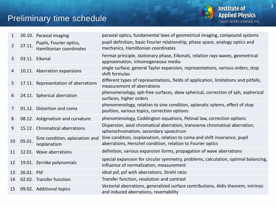
Preliminary time schedule

1 20.10. Paraxial imaging paraxial optics, fundamental laws of geometrical imaging, compound systems

2 27.11. Pupils, Fourier optics, Hamiltonian coordinates

pupil definition, basic Fourier relationship, phase space, analogy optics and mechanics, Hamiltonian coordinates

3 03.11. Eikonal Fermat principle, stationary phase, Eikonals, relation rays-waves, geometrical approximation, inhomogeneous media

4 10.11. Aberration expansions single surface, general Taylor expansion, representations, various orders, stop shift formulas

5 17.11. Representation of aberrations different types of representations, fields of application, limitations and pitfalls, measurement of aberrations

6 24.11. Spherical aberration phenomenology, sph-free surfaces, skew spherical, correction of sph, aspherical surfaces, higher orders

7 01.12. Distortion and coma phenomenology, relation to sine condition, aplanatic sytems, effect of stop position, various topics, correction options

8 08.12. Astigmatism and curvature phenomenology, Coddington equations, Petzval law, correction options

9 15.12. Chromatical aberrations Dispersion, axial chromatical aberration, transverse chromatical aberration, spherochromatism, secondary spoectrum

10 05.01. Sine condition, aplanatism and isoplanatism

Sine condition, isoplanatism, relation to coma and shift invariance, pupil aberrations, Herschel condition, relation to Fourier optics

11 12.01. Wave aberrations definition, various expansion forms, propagation of wave aberrations

12 19.01. Zernike polynomials special expansion for circular symmetry, problems, calculation, optimal balancing, influence of normalization, measurement

13 26.01. PSF ideal psf, psf with aberrations, Strehl ratio

14 02.02. Transfer function Transfer function, resolution and contrast

15 09.02. Additional topics Vectorial aberrations, generalized surface contributions, Aldis theorem, intrinsic and induced aberrations, revertability

1. Material dispersion

2. Partial dispersion

3. Anomalous partial dispersion

4. Axial chromatical error

5. Achromatic

6. Apochromates

7. Spherochromatism

8. Chromatical variation of magnification

9. Examples

3

Contents

refractive

index n

1.65

1.6

1.5

1.8

1.55

1.75

1.7

BK7

SF1

0.5 0.75 1.0 1.25 1.751.5 2.0

1.45

flint

crown

Description of dispersion:

Abbe number

Visual range of wavelengths:

typically d,F,C or e,F’,C’ used

Typical range of glasses

ne = 20 ...100

Two fundamental types of glass:

Crown glasses:

n small, n large, dispersion low

Flint glasses:

n large, n small, dispersion high

n

n

n nF C

1

' '

ne

e

F C

n

n n

1

' '

Dispersion and Abbe number

4

Curvatures cj of the radii of a lens

Focal power at the center wavelength e for a thin lens

Difference in focal powers for outer wavelengths F', C' with the Abbe number

Focal length at the center wavelength

Difference of the focal lengths for outer wavelengths

Achromatization condition for two thin lenses close together

Abbe Number and Achromatization

2

2

1

1

1,

1

rc

rc

cnccnF eee )1())(1( 21

e

ee

e

CFCFCF

Fcn

n

nncnnFFF

n

)1(

1)( ''

''''

cnFf

ee

e

)1(

11

e

e

e

FC

CF

FCCF

f

cn

nn

cnn

nnfff

n

2

''

''

''''

)1()1)(1(

''

1

CF

ee

nn

n

n

011

22112

2

1

1 nnnn ff

FFF

5

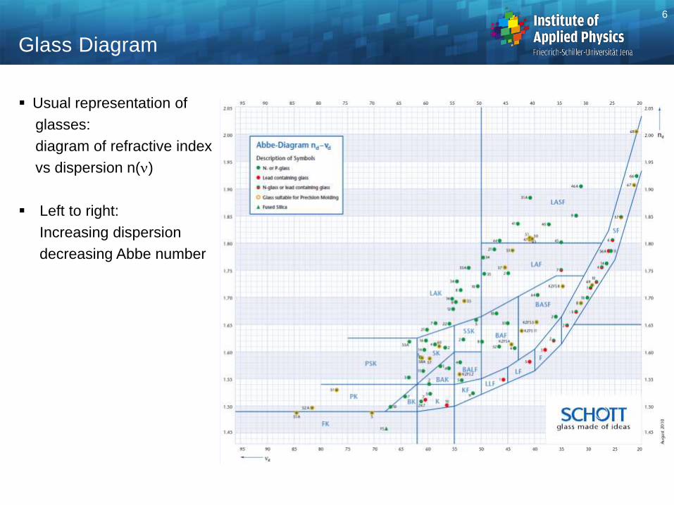
Usual representation of

glasses:

diagram of refractive index

vs dispersion n(n)

Left to right:

Increasing dispersion

decreasing Abbe number

Glass Diagram

6

Material with different dispersion values:

- Different slope and curvature of the dispersion curve

- Stronger change of index over wavelength for large dispersion

- Inversion of index sequence at the boundaries of the spectrum possible

refractive index n

F6

SK18A

1.675

1.7

1.65

1.625

1.60.5 0.75 1.0 1.25 1.751.5 2.0

VIS

flint

n small

slope large

crown

n largeslope small

Dispersion

7

Atomic model for the refractive index: oscillator approach of atomic field interaction

Sellmeier dispersion formula: corresponding function

Special case of coupled resonances: example quartz, degenerated oscillators

Atomic Model of Dispersion

j jjj

jj

iric

f

mc

Nenin

222

22

0

22

22

10-1

100

101

0

1

2

3

4

5

6

7

log

[mm]

nvisible

0.4 0.7

1(UV)

2(UV)

3(IR)

4(IR)

nvis()

j j

j

C

BAn

2

2

2

12

2

222

4

02

j j

j

oC

BBAn

8

Schott formula

empirical

Sellmeier

Based on oscillator model

Bausch-Lomb

empirical

Herzberger

Based on oscillator model

Hartmann

Based on oscillator model

n a a a a a ao

1

2

2

2

3

4

4

6

5

8

n A B C( )

2

212

2

222

n A B CD E

Fo

o

( )

( )

2 4

2

2

2 22

2 2

mmit

aaaan

o

oo

o

m

168.0

)(222

3

22

22

1

5

4

3

1)(a

a

a

aan o

Dispersion formulas

9

Relative partial dispersion :

Change of dispersion slope with

Different curvature of dispersion curve

Definition of local slope for selected

wavelengths relative to secondary

colors

Special -selections for characteristic

ranges of the visible spectrum

= 656 / 1014 nm far IR

= 656 / 852 nm near IR

= 486 / 546 nm blue edge of VIS

= 435 / 486 nm near UV

= 365 / 435 nm far UV

P

n n

n nF C

1 2

1 2

' '

n

400 600 800 1000700500 900 1100

e : 546 nm

main color

F' : 480 nm

1. secondary

color

g : 435 nmUV edge

C' : 644 nm

s : 852 nm

IR edge

t : 1014 nm

IR edge

C : 656 nmF : 486 nm

d : 588 nm

i : 365 nm

UV edge

i - g

F - C

C - s

C - t

F - e

g - F

2. secondary

color

1.48

1.49

1.5

1.51

1.52

1.53

1.54

n()

Relative partial dispersion

10

Partial Dispersion and Normal Line

The relative partial dispersion changes approximately linear with the dispersion for glasses

Nearly all glasses are located on the normal line in a P-n-diagram

The slope of the normal line depends on the selection of wavelengths

Glasses apart from the normal line shows anomalous partial dispersion

P

these material are important for chromatical correction of higher order

2,12,12,1 n baP d

21212121 n PbaP d

PgF

80 60 40 20

0.5

0.6

P

0.55

0.45

PCs

n

11

Anormal partial dispersion and normal line

Partial Dispersion

12

Pg,F

0.5000

0.5375

0.5750

0.6125

0.6500

90 80 70 60 50 40 30 20

F2

F5

K7

K10

LAFN7

LAKN13

LAKL12

LASFN9

SF1

SF10

SF11

SF14

SF15

SF2

SF4

SF5

SF56A

SF57

SF66

SF6

SFL57

SK51

BASF51

KZFSN5

KZFSN4

LF5

LLF1

N-BAF3

N-BAF4

N-BAF10

N-BAF51N-BAF52

N-BAK1

N-BAK2

N-BAK4

N-BALF4

N-BALF5

N-BK10

N-F2

N-KF9

N-BASF2

N-BASF64

N-BK7

N-FK5

N-FK51N-PK52

N-PSK57

N-PSK58

N-K5

N-KZFS2

N-KZFS4

N-KZFS11

N-KZFS12

N-LAF28

N-LAF2

N-LAF21N-LAF32

N-LAF34

N-LAF35

N-LAF36

N-LAF7

N-LAF3

N-LAF33

N-LAK10

N-LAK22

N-LAK7

N-LAK8

N-LAK9

N-LAK12

N-LAK14

N-LAK21

N-LAK33

N-LAK34

N-LASF30

N-LASF31

N-LASF35

N-LASF36

N-LASF40

N-LASF41

N-LASF43

N-LASF44

N-LASF45

N-LASF46

N-PK51

N-PSK3

N-SF1

N-SF4

N-SF5

N-SF6

N-SF8

N-SF10

N-SF15

N-SF19

N-SF56

N-SF57

N-SF64

N-SK10

N-SK11

N-SK14

N-SK15

N-SK16

N-SK18N-SK2

N-SK4

N-SK5

N-SSK2

N-SSK5

N-SSK8

N-ZK7

N-PSK53

N-PSK3

N-LF5

N-LLF1

N-LLF6

BK7G18

BK7G25

K5G20

BAK1G12

SK4G13

SK5G06

SK10G10

SSK5G06

LAK9G15

LF5G15

F2G12

SF5G10

SF6G05

SF8G07

KZFS4G20

GG375G34

n

normal

line

There are some special glasses with a large deviation from the normal line

Of special interest: long crowns and short flints

Anomalous Partial Dispersion

Pg,F

n

line of normal

dispersion

FK51

KZFSN4

LAK8ZKN7

PSK53ALASFN30

FK5

N-SF57

SF1

Pg,F

n

normal line

long crowns

short flints

heavy flints with

character of long

crowns

n

flint

short flintlong crown

crown

13

Anomalous Partial Dispersion

Normal glasses: Partial dispersion changes linear with Abbe number

Definition of P depends on selected wavelengths

Normal line defined by F2 and K7

Deviation from linear behavior: anomalous partial dispersion P

The value of P depends on the wave- length selection

Typical P considered at the red and the blue end of the visible spectrum

Large deviation values P are necessary for apochromatic chromatical correction

21212121 n PbaP d

d

P

n

g'

normal

line

Pg'

dn

real curve

dgi

dFg

deF

dsC

dtC

P

P

P

P

P

n

n

n

n

n

008382.07241.1

001682.06438.0

000526.04884.0

002331.04029.0

004743.05450.0

,

,

,

,

,

14

Arrows in the glass map: indication of the deviation from the

normal line

Vertical component: at the red horizontal: at the blue end of the spectrum

Anomalous Partial Dispersion

d

PhF'

n

normal line

Glass

PhF'

nd

21212121 n PbaP d

n

PtC'

nd

blue side

red side

arrow of

deviation

glass

locationPhF'

15

Axial chromatical aberration:

- dispersion of marginal ray

- different image locations

Transverse chromatical aberration:

- dispersion of chief ray

- different image sizes

16

Chromatical Aberrations

object

chief ray

marginal

ray

chief rays

marginal rays

2

1

ExP

2

ExP

1

transverse

chromatical

aberration

axial

chromatical

aberration

ideal

image

1

ideal

image

2

1. Third order chromatical aberrations:

- axial chromatical aberration

error of the marginal ray by dispersion

- transverse chromatical aberration

error of the chief ray by dispersion

2. Higher order chromatical aberrations:

- secondary spectrum

residual axial error, if only selected wavelength are coinciding

- spherochromatism

chromatical variation of the spherical aberration, observed in an achromate

- chromatical variation of all monochromatic aberrations

e.g. astigmatism, coma, pupil location,...

17

Overview on Chromatical Aberrations

Various cases of chromatical aberration correction

18

Chromatical Aberrations

a) axial and lateral color corrected

CRMRFC

FC

b) axial color corrected

F

FC

C

c) lateral color corrected

F C

F C

d) no color corrected

F

C

F C

Axial Chromatical Aberration

s s sCHL F C' ' '' '

white

P'

s'F'

s'

s'

e

C'green

red

blue

Axial chromatical aberration:

Higher refractive index in the blue results in a shorter intersection length for a single lens

The colored images are defocussed along the axis

Definition of the error: change in image location /

intersection length

Correction needs several glasses with different dispersion

Single lens: normal dispersion

blue intersection length is shorter

than red

Notations:

1. CHL = chromatical longitudinal

2. AXCL = axial chromatic

19

Axial Chromatical Aberration

z

= 648 nm

defocus

-2 -1 0 1 2

= 546 nm

= 480 nm

best image plane

Longitudinal chromatical aberration for a single lens

Best image plane changes with wavelength

Ref : H. Zügge

20

s

e C'F'

Secondary Spectrum

Simple achromatization / first order

correction:

- two glasses with different dispersion

- equal intersection length for outer

wavelengths (blue F', red C')

Residual deviation for middle wavelength

(green e):

secondary spectrum

white

P'

s'F'

s'

s'

e

C'

green

redblue

secondary

spectrum

21

e

F'

C' achromate

644

480

546

residual error

achromate

-100 0 100

singlet

s'

s s s fP P

SSP C

C C' ' ''

, '

( )

, '

( )

n n

1 2

1 2

Achromate: Basic Formulas

Idea:

1. Two thin lenses close together with different materials

2. Total power

3. Achromatic correction condition

Individual power values

Properties:

1. One positive and one negative lens necessary

2. Two different sequences of plus (crown) / minus (flint)

3. Large n-difference relaxes the bendings

4. Achromatic correction indipendent from bending

5. Bending corrects spherical aberration at the margin

6. Aplanatic coma correction for special glass choices

7. Further optimization of materials reduces the spherical zonal aberration

21 FFF

02

2

1

1 nn

FF

FF

1

21

1

1

n

n FF

2

12

1

1

n

n

22

Compensation of axial colour by

appropriate glass choice

Chromatical variation of the spherical

aberrations:

spherochromatism (Gaussian aberration)

Therefore perfect axial color correction

(on axis) are often not feasable

Achromate

BK7 F2

n = 1.5168 1.6200

= 64.17 36.37

F = 2.31 -1.31

BK7 N-SSK8F2

n = 1.5168 1.6177

= 64.17 49.83

F = 4.47 -3.47

BK7

n= 1.5168n = 64.17

F= 1

(a) (b) (c)

-2.5 0z

r p1

-0.20

1

z

0.200

r p

-100 1000

1

r p

z

486 nm

588 nm

656 nm

n n

Ref : H. Zügge

23

Achromate

Achromate

Longitudinal aberration

Transverse aberration

Spot diagram

rp

0

486 nm

587 nm

656 nm

0.1 0.2

s'

[mm]

1

axis

1.4°

2°

486 nm 587 nm 656 nm

= 486 nm

= 587 nm

= 656 nm

sinu'

y'

24

Achromate: Correction

Cemented achromate: 6 degrees of freedom: 3 radii, 2 indices, ratio n1/n2

Correction of spherical aberration: diverging cemented surface with positive spherical contribution for nneg > npos

Choice of glass: possible goals 1. aplanatic coma correction 2. minimization of spherochromatism 3. minimization of secondary spectrum Bending has no impact on chromatical correction: is used to correct spherical aberration at the edge Three solution regions for bending 1. no spherical correction 2. two equivalent solutions 3. one aplanatic solution, very stable

case without solution,

only spherical minimum

case with

2 solutions

case with

one solution

and coma

correction

sMR'

R1

aplanatic

case

Achromatic Solutions in the Glass Diagram

Achromat

flint

negative lens

crown

positive lens

large n-differences

give relaxed bendings

26

For one given flint a line indicates the usefull crown glasses and vice versa

Perfect aplanatic line of corresponding glasses (corrected for coma)

Condition:

Optimization of Achromatic Glasses

n

n

fixed flint glass

line of

minimal

spherical

aberration

n

nfixed crown glass

line of

minimal

spherical

aberration

11

11

'

11

2

2

2

1

2

2

11

21

2

2

2

2

1

1

1

22

2n

nn

n

n

n

n

srn

n

n

n

n

nn

n

n

n

27

Achromate

Residual aberrations of an achromate

Clearly seen:

1. Distortion

2. Chromatical magnification

3. Astigmatism

28

Surface and Lens contribution of Axial Color

Considering the Abbe invariant

Derivative after the wavelength

Summing over all surfaces of a system with the marginal ray height ratio and the propagation of the ratio

Surface summation for axial chromatical aberration

with the surface contribution coefficient

1h

h j

j j

j

jjs

s

'

1

1

d

ds

s

n

srd

dn

d

ds

s

n

srd

dn j

j

j

jj

jj

j

j

jj

j

22

11'

'

'

'

11'

jj

j

jj

j

jj

srn

srn

QQ

11

'

11'

'

j

j

jj

j

jj

j

NN

NCHL n

srn

srn

ss

11'

'

11

'

'' 2

2

2

N

j

CHL

j

NN

NN

j jj

j

jj

j

jj

NN

nCHL K

n

s

n

n

n

nQ

n

ss

12

2

1

2

2

2

'

'1

'

1'

'

''

nn

jj

j

jj

j

jj

CHL

jn

n

n

nQK

nn

1

''

1'2

29

General Achromatization

Contribution of a thin lens to the axial chromatical aberration

Axial chromatical aberration of a system of thin lenses

Condition of achromatization of a system of lenses

Special case of lenses close together

Condition of apochromatic (polychromatic) correction with the partial relative dispersion

jj

j

j

j

j

CHL

lensf

FK

n

n

'

2

2

j j

j

j

N

CHL

Fss

n

2

2

2''

02 j j

j

j

F

n

02

j j

jj

j

FP

n

0j j

jF

n

30

Dialyt approach: Achromatization with two lenses at finite distance

Scaling parameter k:

With finite marginal ray height

Focal length condition

Achromatization

Focal lengths of the lenses

Lens distance

af

tk

'

ba f

k

ff

111

022

bb

b

aa

a

f

y

f

y

nn

kff

a

ba

11

n

n

b

ab

kkff

n

n 111

fk

kda

b

)1(1

n

n

Dialyt-Achromat

31

Usage of only one glass material with achromatic correction: dialyt achromate

No real imaging possible

Parameters:

Setup

lens b

lens a

ay

yb

t

f a

s'

image

plane

1

k

kffa )1( kfkfb

fk

kt

1

2

Dialyt Achromat

32

Special layout of dialyte approach according to Schupman

Mirror guarantees real imaging

Axial Color Correction with Schupman Lens

f1 = 300 mm

f2 = -100 mm

mirror

real image

33

Choice of at least one special glass

Correction of secondary spectrum:

anomalous partial dispersion

At least one glass should deviate

significantly form the normal glass line

Axial Colour : Apochromate

656nm

588nm

486nm

436nm1mm

z0-0.2mm

z-0.2mm

2030405060708090

N-FK51

N-KZFS11

N-FS6

(1)

(2)

(3)

(1)+(2) T

PgF

0,54

0,56

0,58

0,60

0,62

n

34

Focal power condition

Achromatic condition

Secondary spectrum

Curvatures of lenses

Parameter E

The 3 materials are not allowed to be on the normal line

The triangle of the 3 points should be large: small cj give relaxed design

321 FFFF

03

3

2

2

1

1 nnn

FFF

03

33

2

22

1

11

nnn

FPFPFP

21

11

rrc

3,1,

1

nn aa

cb

ca

ann

PP

Efc

3,1,

1

nn bb

ac

ca

bnn

PP

Efc

3,1,

1

nn cc

ba

ca

cnn

PP

Efc

bacacbcba

ca

PPPPPPE

nnnnn

1

Apochromate

35

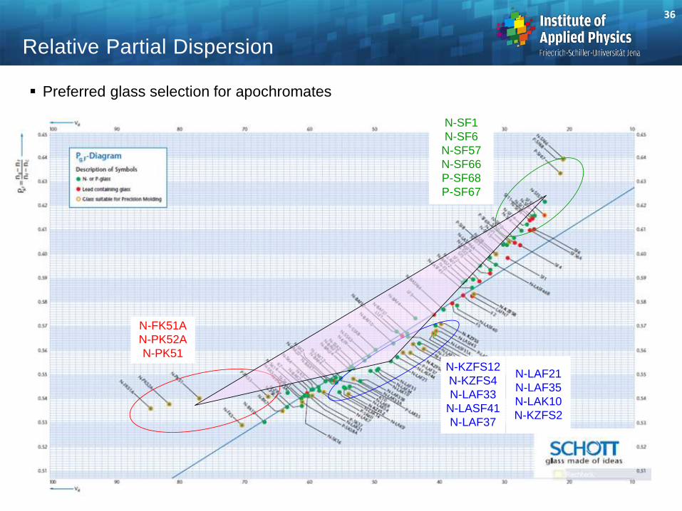
Preferred glass selection for apochromates

36

Relative Partial Dispersion

N-SF1

N-SF6

N-SF57

N-SF66

P-SF68

P-SF67

N-FK51A

N-PK52A

N-PK51

N-KZFS12

N-KZFS4

N-LAF33

N-LASF41

N-LAF37

N-LAF21

N-LAF35

N-LAK10

N-KZFS2

Effect of different materials

Axial chromatical aberration

changes with wavelength

Different levels of correction:

1.No correction: lens,

one zero crossing point

2.Achromatic correction:

- coincidence of outer colors

- remaining error for center

wavelength

- two zero crossing points

3. Apochromatic correction:

- coincidence of at least three

colors

- small residual aberrations

- at least 3 zero crossing points

- special choice of glass types

with anomalous partial

dispertion necessery

Axial Colour: Achromate and Apochromate

e

F'

C'

achromateapochromate

residual error

apochromate

644

480

546

residual error

achromate

-100 0 100

singlet

s'

lens

37

Spherochromatism

Spherochromatism: variation of spherical aberration with wavelength, Alternative notation: Gaussian chromatical error

Individual curve of spherical aberration with color

Conventional achromate: - coinciding image location for red (C‘) and blue (F‘) on axis (paraxial)

- differences and secondary spectrum for green (e)

- but different intersection lengths

for finite aperture rays

Better balancing with half spherochromatism on axis

0

aperture

1

0.1 mm

480 nm

546 nm

644 nm

s'sec

s'tot

0.2 mm

s'

rp

1

0.5

0 0.40.2 0.6-0.2

546 nm

480

nm

644 nm

s' in

RU

s'chl

38

Spherical aberration of a

lens in 3rd order:

Wavelength dependence of n induces spherochromatism

Typical spectral variation of this aberration with wavelength

Spherochromatism

A

n n f

n

n

n

nX

n

nM

n n

nMs

1

32 1 1

2

1

2 1

2

1

23

3 22

2

2

( )

z

-1

+1

0.48 0.644

a) single lens

z

-1.5

+1.5

0.48 0.644

b) corrected

39

Conventional achromate: strong bending of image shell, typical

Special selection of glasses:

1. achromatization

2. Petzval flattening

Residual field curvature:

Combined condition

But usually no spherical correction possible

'

111

2

2

1

1

12 fnnRptz

nn

nn

'3.1 fRptz

New Achromate

perfect

image

plane

Petzval

shell

y'

f

RP

mean

image shell

2

1

2

1

n

n

n

n

02

2

1

1 n

n

FF

02

2

1

1 n

F

n

Fn

n

selected crown glass

line of solutionfor flint glass

40

Principles of Glass Selection in Optimization

field flattening

Petzval curvature

color

correction

index n

dispersion n

positive

lens

negative

lens

-

-

+

-

+

+

availability

of glasses

Design rules for glass selection

Different design goals:

1. Color correction:

large dispersion

difference desired

2. Field flattening:

large index difference

desired

Ref : H. Zügge

41

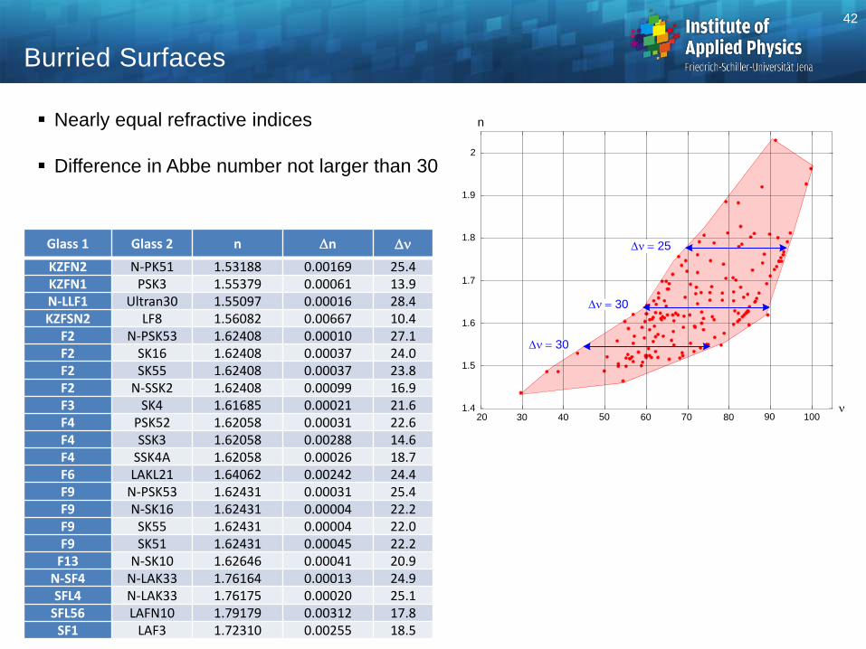
Nearly equal refractive indices

Difference in Abbe number not larger than 30

Burried Surfaces

n

n

20 30 40 50 60 70 80 90 1001.4

1.5

1.6

1.7

1.8

1.9

2

n 30

n 30

n 25Glass 1 Glass 2 n n n

KZFN2 N-PK51 1.53188 0.00169 25.4

KZFN1 PSK3 1.55379 0.00061 13.9

N-LLF1 Ultran30 1.55097 0.00016 28.4

KZFSN2 LF8 1.56082 0.00667 10.4

F2 N-PSK53 1.62408 0.00010 27.1

F2 SK16 1.62408 0.00037 24.0

F2 SK55 1.62408 0.00037 23.8

F2 N-SSK2 1.62408 0.00099 16.9

F3 SK4 1.61685 0.00021 21.6

F4 PSK52 1.62058 0.00031 22.6

F4 SSK3 1.62058 0.00288 14.6

F4 SSK4A 1.62058 0.00026 18.7

F6 LAKL21 1.64062 0.00242 24.4

F9 N-PSK53 1.62431 0.00031 25.4

F9 N-SK16 1.62431 0.00004 22.2

F9 SK55 1.62431 0.00004 22.0

F9 SK51 1.62431 0.00045 22.2

F13 N-SK10 1.62646 0.00041 20.9

N-SF4 N-LAK33 1.76164 0.00013 24.9

SFL4 N-LAK33 1.76175 0.00020 25.1

SFL56 LAFN10 1.79179 0.00312 17.8

SF1 LAF3 1.72310 0.00255 18.5

42

Cemented component with plane outer surfaces

For center wavelength only plane parallel plate, not seen in collimated light

Curved cemeneted surface:

- dispersion for outer spectral weavelengths

- color correction without disturbing the main wavelength

Example

Burried Surfaces

n

n1

n

n2

green undeflected

a) singlet

-320 -160 0 160 3200.480

0.530

0.580

0.630

z

b) color corrected

corrected

singlet

43

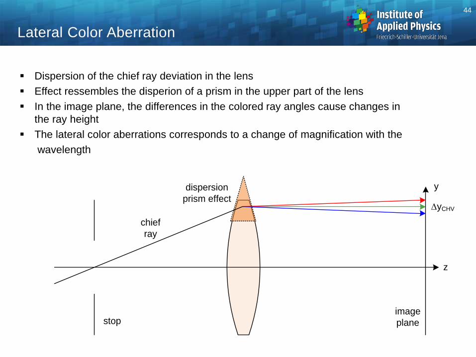
Lateral Color Aberration

Dispersion of the chief ray deviation in the lens

Effect ressembles the disperion of a prism in the upper part of the lens

In the image plane, the differences in the colored ray angles cause changes in

the ray height

The lateral color aberrations corresponds to a change of magnification with the

wavelength

z

y

stop

dispersion

prism effect

image

plane

yCHV

chief

ray

44

stop

red

blue

reference

image

plane

y'CHV

'' ''' CFCHV yyy

e

CFCHV

y

yyy

'

''' ''

Chromatic Variation of Magnification

Lateral chromatical aberration:

Higher refractive index in the blue results in a stronger

ray bending of the chief ray for a single lens

The colored images have different size,

the magnification is wavelength dependent

Definition of the error: change in image height/magnification

Correction needs several glasses with different dispersion

The aberration strongly depends on the stop position

45

Surface and Lens contribution of Lateral Color

If the imaging of the entrance to the exit pupil suffers from axial chromatical aberrations, this delivers an error of the exit pupil location and also of the chief ray angle: cheomatical lateral aberration

Transverse chromatical aberration of a lens system

Surface contribution coefficient of lateral color

Corresponding lens summation formula

jj

j

jj

j

pjpjj

p

pCHV

jn

n

n

nQ

ss

ssH

nn

1

''

1'

11

11

y y HCHV n j

CHV

j

n

' '

1

n

j jj

j

pjpjj

p

p

nCHVn

nQ

ss

ssyy

111

11 1''

n

n

j j

j

pjj

p

p

nCHV

F

ss

ssyy

111

11''

n

46

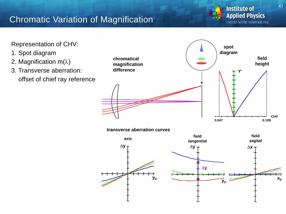
Chromatic Variation of Magnification

Representation of CHV:

1. Spot diagram

2. Magnification m()

3. Transverse aberration:

offset of chief ray reference

spot

diagram

transverse aberration curves

chromatical

magnification

difference

0.047 CHV

Y‘

0.108

axisfield

tangential

field

sagital

field

height

y

y

ypyp

xp

xy

47

Impression of CHV in real images

Typical colored fringes blue/red at edges visible

Color sequence depends on sign of CHV

Chromatic Variation of Magnification

original

without

lateral

chromatic

aberration

0.5 % lateral

chromatic

aberration

1 % lateral

chromatic

aberration

48

Chromatical Difference in Magnification

Color rings are hardly seen due

to colored image

Lateral shift of colored psf positions

Ref: J. Kaltenbach

49

Axial Chromatical Aberration

Special effects near black-white edges

boarder

magenta

blue boarder

Ref: J. Kaltenbach

50

Lateral Color Correction: Principle of Symmetry

Perfect symmetrical system: magnification m = -1

Stop in centre of symmetry

Symmetrical contributions of wave aberrations are doubled (spherical)

Asymmetrical contributions of wave aberration vanishes W(-x) = -W(x)

Easy correction of:

coma, distortion, chromatical change of magnification

front part rear part

2

1

3

51