loss of phase and universality of stochastic interactions ...fibich/manuscripts/lop-oe17.pdf ·...

Loss of phase and universality of stochasticinteractions between laser beams

AMIR SAGIV,* ADI DITKOWSKI, AND GADI FIBICH

Department of Applied Mathematics, Tel Aviv University, Tel Aviv 6997801, Israel*[email protected]

Abstract: Traditionally, interactions between laser beams or filaments were considered to bedeterministic. We show, however, that in most physical settings, these interactions ultimatelybecome stochastic. Specifically, we show that in nonlinear propagation of laser beams, the shot-to-shot variation of the nonlinear phase shift increases with distance, and ultimately becomesuniformly distributed in [0, 2π]. Therefore, if two beams travel a sufficiently long distancebefore interacting, it is not possible to predict whether they would intersect in- or out-of-phase. Hence, if the underlying propagation model is non-integrable, deterministic predictionsand control of the outcome of the interaction become impossible. Because the relative phasebetween the two beams becomes uniformly distributed in [0, 2π], however, the statistics of thesestochastic interactions are universal and fully predictable. These statistics can be efficientlycomputed using a novel universal model for stochastic interactions, even when the noise dis-tribution is unknown.

c© 2017 Optical Society of America

OCIS codes: (190.3270) Kerr effect; (350.5030) Phase; (260.3160) Interference; (190.3100) Instabilities and chaos;

(140.3298) Laser beam combining.

References and links1. G. Stegeman and M. Segev, “Optical spatial solitons and their interactions: universality and diversity,” Science 286,

1518–1523 (1999).2. A. Skidin, O. Sidelnikov, M. Fedoruk, and S. Turitsyn, “Mitigation of nonlinear transmission effects for OFDM

16-QAM optical signal using adaptive modulation,” Opt. Express 24, 30296–30308 (2016).3. T. Y. Fan, “Laser beam combining for high-power, high-radiance sources,” IEEE J. Sel. Top. Quantum Electron. 11,

567–577 (2005).4. L. Daniault, S. Bellanger, J. Le Dortz, J. Bourderionnet, É. Lallier, C. Larat, M. Antier-Murgey, J. Chanteloup,

A. Brignon, and C. Simon-Boisson, “Xcan—a coherent amplification network of femtosecond fiber chirped-pulseamplifiers,” Europ. Phys. J. Special Topics 224, 2609–2613 (2015).

5. G. Mourou, T. Tajima, M. Quinn, B. Brocklesby, and J. Limpert, “Are fiber-based lasers the future of accelerators?”Nucl. Instrum. Methods Phys. Res. Sect. A 740, 17–20 (2014).

6. G. Mourou, B. Brocklesby, T. Tajima, and J. Limpert, “The future is fibre accelerators,” Nat. Photon. 7, 258–261(2013).

7. C. Bellanger, B. Toulon, J. Primot, L. Lombard, J. Bourderionnet, and A. Brignon, “Collective phase measurementof an array of fiber lasers by quadriwave lateral shearing interferometry for coherent beam combining,” Opt. Lett.35, 3931–3933 (2010).

8. A. Couairon and A. Mysyrowicz, “Femtosecond filamentation in transparent media,” Phys. Rep. 441, 47–189(2007).

9. H. Frostig, E. Small, S. Derevyanko, and Y. Silberberg, “Focusing coherent light through a nonlinear scatteringmedium,” arXiv preprint arXiv:1607.08105 (2016).

10. W. Kruer, S. Wilks, B. Afeyan, and R. Kirkwood, “Energy transfer between crossing laser beams,” Phys. Plasmas3, 382–385 (1996).

11. V. Zakharov and A. Shabat, “Interaction between solitons in a stable medium,” Sov. Phys. JETP 37, 823–828 (1973).12. M. Ablowitz, B. Prinari, and A. Trubatch, Discrete and Continuous Nonlinear Schrödinger Systems (Cambridge

University, 2004).13. F. M. Mitschke and L. F. Mollenauer, “Experimental observation of interaction forces between solitons in optical

fibers,” Opt. Lett. 12, 355–357 (1987).14. A. Snyder and A. Sheppard, “Collisions, steering, and guidance with spatial solitons,” Opt. Lett. 18, 482–484

(1993).15. S. Tzortzakis, L. Bergé, A. Couairon, M. Franco, B. Prade, and A. Mysyrowicz, “Breakup and fusion of self-guided

femtosecond light pulses in air,” Phys. Rev. Lett. 86, 5470–5473 (2001).

Vol. 25, No. 20 | 2 Oct 2017 | OPTICS EXPRESS 24387

#297409 https://doi.org/10.1364/OE.25.024387 Journal © 2017 Received 21 Jun 2017; revised 8 Sep 2017; accepted 8 Sep 2017; published 26 Sep 2017

16. V. Tikhonenko, J. Christou, and B. Luther-Davies, “Three dimensional bright spatial soliton collision and fusion ina saturable nonlinear medium,” Phys. Rev. Lett. 76, 2698 (1996).

17. G. Garcia-Quirino, M. Iturbe-Castillo, V. Vysloukh, J. Sanchez-Mondragon, S. Stepanov, G. Lugo-Martinez, andG. Torres-Cisneros, “Observation of interaction forces between one-dimensional spatial solitons in photorefractivecrystals,” Opt. Lett. 22, 154–156 (1997).

18. A. Ishaaya, T. Grow, S. Ghosh, L. Vuong, and A. Gaeta, “Self-focusing dynamics of coupled optical beams,” Phys.Rev. A 75, 023813 (2007).

19. A. C. Scott, F. Chu, and D. W. McLaughlin, “The soliton: A new concept in applied science,” Proc. IEEE 61,1443–1483 (1973).

20. Y. S. Kivshar and B. A. Malomed, “Dynamics of solitons in nearly integrable systems,” Rev. Mod. Phys. 61, 763(1989).

21. G. Agrawal, Nonlinear Fiber Optics (Academic, 2007).22. J. Gordon, “Interaction forces among solitons in optical fibers,” Opt. Lett. 8, 596–598 (1983).23. J. Meier, G. Stegeman, Y. Silberberg, R. Morandotti, and J. Aitchison, “Nonlinear optical beam interactions in

waveguide arrays,” Phys. Rev. Lett. 93, 093903 (2004).24. A. Craik, Wave Interactions and Fluid Flows (Cambridge University, 1988).25. C. Su and R. M. Mirie, “On head-on collisions between two solitary waves,” J. Fluid Mech. 98, 509–525 (1980).26. N. Zabusky and M. Kruskal, “Interaction of solitons in a collisionless plasma and the recurrence of initial states,”

Phys. Rev. Lett. 15, 240 (1965).27. J. H. Nguyen, P. Dyke, D. Luo, B. Malomed, and R. Hulet, “Collisions of matter-wave solitons,” Nat. Phys. 10,

918–922 (2014).28. G. Fibich and M. Klein, “Continuations of the nonlinear Schrödinger equation beyond the singularity,” Nonlinearity

24, 519–552 (2011).29. F. Merle, “On uniqueness and continuation properties after blow-up time of self-similar solutions of nonlinear

Schrödinger equation with critical exponent and critical mass,” Comm. Pure Appl. Math. 45, 203–254 (1992).30. B. Shim, S. Schrauth, A. Gaeta, M. Klein, and G. Fibich, “Loss of phase of collapsing beams,” Phys. Rev. Lett. 108,

043902 (2012).31. A. Goy and D. Psaltis, “Imaging in focusing Kerr media using reverse propagation [invited],” Phot. Res. 1, 96–101

(2013).32. C. Barsi, W. Wan, and J. Fleischer, “Imaging through nonlinear media using digital holography,” Nat. Photon. 3,

211–215 (2009).33. G. Fibich, The Nonlinear Schrödinger Equation (Springer, 2015).34. C. Rotschild, O. Cohen, O. Manela, M. Segev, and T. Carmon, “Solitons in nonlinear media with an infinite Range

of nonlocality: First observation of coherent elliptic solitons and of vortex-ring solitons,” Phys. Rev. Lett. 95 213904(2005)

35. Q. Quo, B. Luo, F. Yi, S. Chi, and Y. Xie, “Large phase shift of nonlocal optical spatial solitons,” Phys. Rev. E 69,016602 (2004)

36. K. G. Makris, R. El-Ganainy, D. N. Christodoulides, and Z. H. Musslimani, “PT-Symmetric periodic opticalpotentials,” Int. J. Theor. Phys. 50, 1019–1041 (2011)

37. F. K. Abdullaev, Y. V. Kartashov, V. V. Konotop, and D. A. Zezyulin, “Solitons in PT-symmetric nonlinear lattices,”Phys. Rev. A 83, 041805 (2011)

38. M. Wimmer, A. Regensburger, M. A. Miri, C. Bersch, D. N. Christdoulides, and U. Peschel, “Observation of opticalsolitons in PT-symmetric lattices,” Nat. Comm. 6, 7782 (2015)

39. T. Cazenave, and P. L. Lions, “Orbital stability of standing waves for some nonlinear Schrödinger equations,” Comm.Math. Phys. 85, 549–561 (1982)

40. M. I. Weinstein, “Modulational stability of ground states of nonlinear Schrödinger equations,” SIAM J. Math. Anal.16, 472–491 (1985)

41. P. Walters, An Introduction to Ergodic Theory, vol. 79 (Springer, 2000).42. W. Królikowski and S. A. Holmstrom, “Fusion and birth of spatial solitons upon collision,” Opt. Lett. 22, 369–371

(1997).43. C. Canuto and A. Quarteroni, “Approximation results for orthogonal polynomials in Sobolev spaces,” Math. Comp.

38, 67–86 (1982).44. D. Day and L. Romero, “Roots of polynomials expressed in terms of orthogonal polynomials,” SIAM J. Numer.

Anal. 43, 1969–1987 (2005).45. A. O’Hagan, “Polynomial chaos: A tutorial and critique from a statistician’s perspective,” SIAM/ASA J. Uncertainty

Quantification 20, 1–20 (2013).46. D. Xiu, Numerical Methods for Stochastic Computations: a Spectral Method Approach (Princeton University,

2010).47. Z. Musslimani, M. Soljacic, M. Segev, and D. Christodoulides, “Delayed-action interaction and spin-orbit coupling

between solitons,” Phys. Rev. Lett. 86, 799 (2001).48. G. Patwardhan, X. Gao, A. Dutt, J. Ginsberg, and A. Gaeta, “Loss of polarization in collapsing beams of elliptical

polarization,” in CLEO: QELS_Fundamental Science (Optical Society of America, 2017), pp. FM3F–7.


1. Introduction

Nonlinear interactions between two or more laser beams, pulses, and filaments [1] are relatedto applications ranging from modulation methods in optical communication [2], to coherentcombination of beams [3–7], interactions between filaments in atmospheric propagation [8],focusing of multiple speckle patterns [9] and ignition of nuclear fusion using up to 192beams [10]. In the integrable one-dimensional cubic case, such interactions can only leadto phase and lateral shifts, which can be computed analytically using the Inverse ScatteringTransform [11–13]. In the non-integrable case, however, richer dynamics are possible, includingbeam repulsion, breakup, fusion and spiraling [1, 14–16]. Since the outcome of the interactionstrongly depends on the relative phases of the beams [17], one can use the initial phase to controlthe interaction dynamics [18]. Nonlinear interactions between solitary waves were also studiedin other physical systems [19, 20], such as fiber optics [21, 22], waveguide arrays [23], waterwaves [24, 25], plasma waves [26] and Bose-Einstein condensates [27].

In previous studies it was shown, both theoretically and experimentally, that when a laserbeam undergoes an optical collapse, its initial phase is "lost", in the sense that the small shot-to-shot variations in the input beam lead to large changes in the nonlinear phase shift of thecollapsing beam [28,29]. Therefore, if two such beams intersect after they collapsed, one cannotpredict whether they will intersect in- or out-of-phase, and so post-collapse interactions betweenbeams become "chaotic" and cannot be controlled [30]. Loss of phase due to input noise canalso interfere with imaging and holography in nonlinear medium [31, 32]. Note that loss ofphase does not imply a loss of coherence, but rather that at any given propagation distance,the coherent beam can only be determined up to an unknown constant phase. Thus, if theunperturbed beam profile is given by ψ = AeiS , then in the presence of input noise ψ = Aei S ,where A(z, x) ≈ A(z, x), S(z, x) ≈ S(z, x) + θ(z), and θ is an unknown O(1) perturbation ofthe nonlinear phase shift which varies with the propagation distance z but is independent of thetransverse coordinates x.

In this study we show that loss of phase is ubiquitous in nonlinear optics. Thus, whilecollapse accelerates the loss of phase process, non-collapsing or mildly-collapsing beams canalso undergo a loss of phase. The loss of phase builds up gradually with the propagation distance,i.e., the shot-to-shot variations of the beam’s nonlinear phase shift increase with the propagationdistance, and approach a uniform distribution in [0, 2π] at sufficiently large distances. As noted,because of the loss of phase, deterministic predictions and control of interactions between laserbeams become impossible in the presence of noise. We show, however, that loss of phase allowsfor accurate predictions of the statistical properties of these stochastic interactions, even withoutany knowledge of the noise source and characteristics. Indeed, because the relative phasebetween the beams becomes uniformly distributed in [0, 2π], the statistics of the interactionare universal, and can be computed using a "universal model" in which the only noise source isa uniformly distributed phase difference between the input beams. These computations can beefficiently performed using a polynomial-chaos based approach.

2. Loss of phase

The propagation of laser beams in a homogeneous medium is governed by the dimensionlessnonlinear Schrödinger equation (NLS) in d + 1 dimensions

i∂

∂zψ(z, x) + ∇2ψ + N ( |ψ |)ψ = 0 , (1)

where z is the dimensionless propagation distance (in units of the diffraction length),x = (x1 , . . . , xd ) are the transverse coordinates (and/or time in the anomalous regime),and ∇2 = ∂2

x1+ · · · + ∂2

xd[33]. Here we consider nonlinearities N (ψ) that support stable


solitary waves ψ = eiκz Rκ (x), such as the cubic-quintic NLS

i∂

∂zψ(z, x) + ∇2ψ + |ψ |2ψ − ε |ψ |4ψ = 0 , (2)

the saturated NLS

i∂

∂zψ(z, x) + ∇2ψ +

|ψ |21 + ε |ψ |2ψ = 0 ,

and certain non-local nonlinearities [34, 35] or PT-symmetric systems [36–38].

2.1. Numerical observations

In a physical system the input beam always changes from shot to shot due to noise andinstabilities of the laser system. To model this shot to shot variation, we write

ψ(z = 0, x; α) = ψ0(x; α) , (3)

where α is the noise realization. We denote by ϕ(z; α) := argψ(z, x = 0; α) the cumulativeon-axis phase at z, and study the evolution (in z) of the probability distribution function (PDF)of the non-cumulative on-axis phase

ϕ(z; α) := ϕ(z; α) mod(2π) . (4)

−1 10

25z = 0.15

α

ϕ(a1)

−1 130

55z = 3

α

(b1)

−1 1105

130z = 11

α

(c1)

−1 10

2π

α

ϕ(a2)

−1 10

2π

α

(b2)

−1 10

2π

α

(c2)

0 2π

f

ϕ

302π

0

(a3)

0 2πϕ

12π

0

(b3)

0 2πϕ

12π

0

(c3)

−4 40

6

x

|ψ|(a4)

−4 40

6

x

(b4)

−4 40

6

x

(c4)

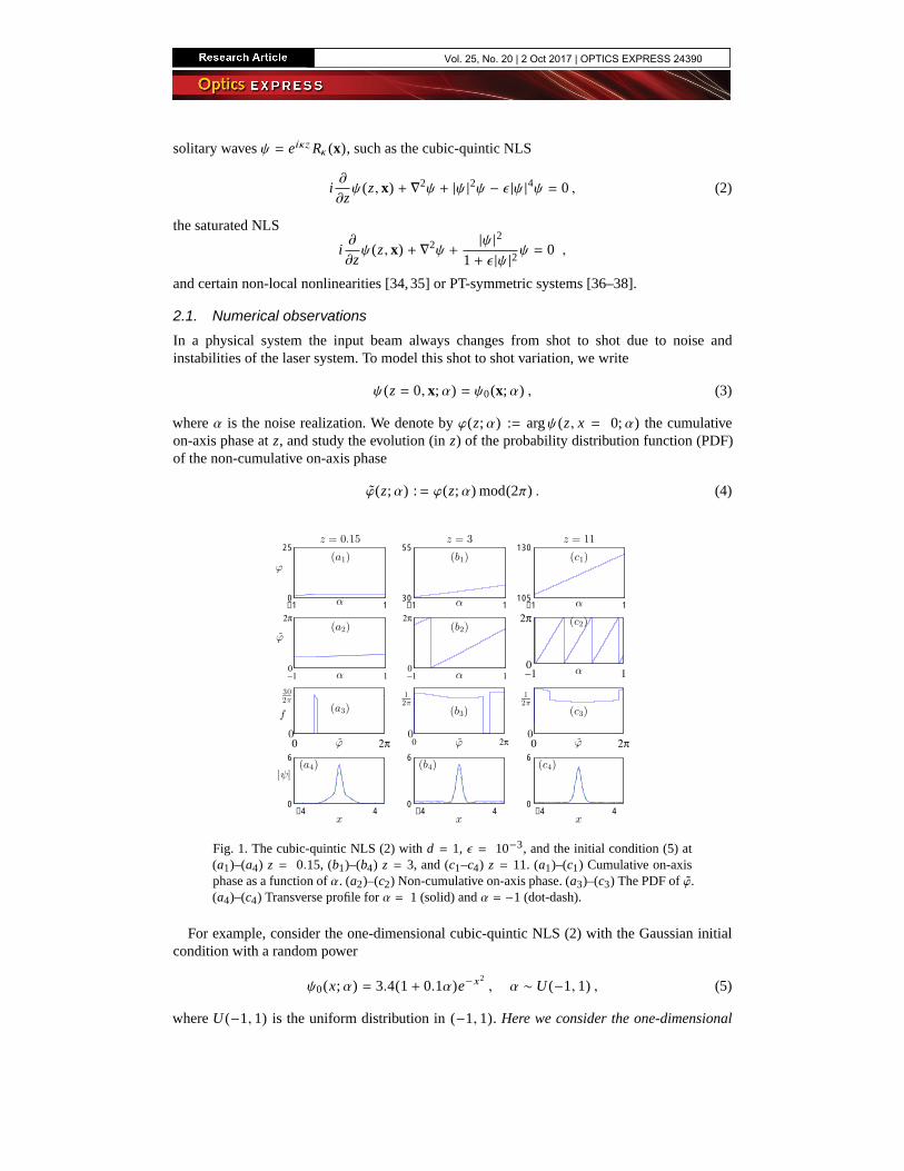
Fig. 1. The cubic-quintic NLS (2) with d = 1, ε = 10−3, and the initial condition (5) at(a1)–(a4) z = 0.15, (b1)–(b4) z = 3, and (c1–c4) z = 11. (a1)–(c1) Cumulative on-axisphase as a function of α. (a2)–(c2) Non-cumulative on-axis phase. (a3)–(c3) The PDF of ϕ.(a4)–(c4) Transverse profile for α = 1 (solid) and α = −1 (dot-dash).

For example, consider the one-dimensional cubic-quintic NLS (2) with the Gaussian initialcondition with a random power

ψ0(x; α) = 3.4(1 + 0.1α)e−x2, α ∼ U (−1, 1) , (5)

where U (−1, 1) is the uniform distribution in (−1, 1). Here we consider the one-dimensional


case to emphasize that loss of phase and "chaotic" interactions are not limited to collapsingbeams, as was implied by earlier studies [28]. At z = 0.15, the maximal variation of thecumulative phase Δϕ := ϕ(α = 1) − ϕ(α = −1) is fairly small (≈ 0.08π), see Fig. 1(a1).The corresponding non-cumulative on-axis phase ϕ(α) is identical (Fig. 1(a2)). Because αis randomly distributed, so is ϕ(α). The probability distribution function (PDF) of ϕ can becomputed from that of α. Since in this example α ∼ U (−1, 1) and the variation in ϕ at z = 0.15is small, the PDF of ϕ, denoted by f (ϕ), is fairly localized, see Fig. 1(a3). As the beam continuesto propagate (z = 3), the maximal variation of the cumulative phase increases to Δϕ ≈ 1.8π, andso ϕ attains most values in [0, 2π], though not with the same probability (Figs. 1(b1)– 1(b3)).At an even larger propagation distance (z = 11), the maximal phase variation is Δϕ ≈ 6.5π,i.e., slightly over three cycles of ϕ, see Figs. 1(c1)–1(c2). At this stage ϕ is nearly uniformly dis-tributed in [0, 2π], see Fig. 1(c3), which implies that the beam "lost" its initial phase ϕ(z = 0).By "loss of phase" we mean that one cannot infer from f , the PDF of ϕ(z; α), or from several

realizations{ϕ(z; α j

}Jj=1

, whether the initial condition was ψ0(x), see (5) or eiθψ0(x) for some

0 < θ < 2π. Loss of phase is not accompanied by a "loss of amplitude". Indeed, the differencesbetween the profiles for α = ±1 remain small throughout the propagation (Figs. 1(a4)– 1(c4)).

We obtained similar results for the same equation and initial condition in two dimensions. Wefound that loss of phase occurs much faster in two dimensions, so that the ϕ becomes uniformlydistributed already after two diffraction lengths (z ≈ 2). See Appendix A for further details.

z

x

(a)

0 7

3

0

−30 7

0

80

ϕ

(b)

z

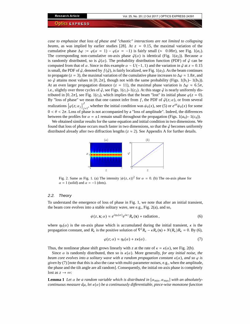
Fig. 2. Same as Fig. 1. (a) The intensity |ψ(z, x) |2 for α = 0. (b) The on-axis phase forα = 1 (solid) and α = −1 (dots).

2.2. Theory

To understand the emergence of loss of phase in Fig. 1, we note that after an initial transient,the beam core evolves into a stable solitary wave, see e.g., Fig. 2(a), and so,

ψ(z, x; α) ≈ eiη0 (α)eiκz Rκ (x) + radiation , (6)

where η0(α) is the on-axis phase which is accumulated during the initial transient, κ is thepropagation constant, and Rκ is the positive solution of ∇2Rκ − κRκ (x) + N (Rκ )Rκ = 0. By (6),

ϕ(z; α) ≈ η0(α) + zκ(α) . (7)

Thus, the nonlinear phase shift grows linearly with z at the rate of κ = κ(α), see Fig. 2(b).Since α is randomly distributed, then so is κ(α). More generally, for any initial noise, the

beam core evolves into a solitary wave with a random propagation constant κ(α), and so ϕ isgiven by (7) [note that this is also the case with multi-parameter noises, e.g., when the amplitude,the phase and the tilt angle are all random]. Consequently, the initial on-axis phase is completelylost as z → ∞:

Lemma 1 Let α be a random variable which is distributed in [αmin , αmax] with an absolutely-continuous measure dμ, let κ(α) be a continuously differentiable, piece-wise monotone function


on [αmin , αmax], let η0(α) be continuously differentiable on [αmin , αmax], and let ϕ be givenby (7). Then

limz→∞ ϕ(z; α) mod (2π) ∼ U ([0, 2π]) .

Proof: see Appendix B .Lemma 1 provides a new road to the emergence of loss of phase. Indeed, in previous

studies [28–30], the loss of phase was caused by the large self-phase modulations (SPM) thataccumulate during the initial beam collapse (i.e., by the variation of η0 in α). Briefly, when abeam undergoes collapse, then in the absence of a collapse-arresting mechanism, ϕ0(α) → ∞ asz → Zc (α), where Zc is the collapse point [28]. Therefore, if a beam undergoes a considerableself-focusing before its collapse is arrested, then it accumulates significant SPM, i.e., η0(α) �2π. In that case, although small changes in α lead to small relative changes in η0(α), those areO(1) absolute changes in η0(α). In this study, however, we consider non-collapsing beams of the1D NLS, or self-trapped beams of the 2D NLS. Therefore Δη0 := η0(αmax) − η0(αmin) 2π.In such cases, the loss of phase builds up gradually with the propagation distance z, and notabruptly during the initial collapse, as in the previous studies.

Loss of phase is related to the fact that NLS solitary waves can "only" be orbitally stable; i.e.,stable up to multiplication by eiθ for some θ ∈ [0, 2π], see [39,40]. Loss of phase is a genuinely

nonlinear phenomenon. Indeed, in the linear propagation regime, ψ(z, x) = (2iz)− 12 eu

|x |24z ∗

ψ0(x). Therefore if ψ0(α1) − ψ0(α2) 1 then ψ(α1) − ψ(α2) 1 as well.Lemma 1 is reminiscent of classical results in ergodic theory of irrational rotations of the

circle [41]. Unlike these results, however, Lemma 1 does not describe the trajectory of a singlepoint on the circle under consecutive discrete phase additions, but rather the convergence of acontinuum of points under with continuous linear change with a varying rate κ.

By (7), the maximal difference in the cumulative phase between solutions grows linearly in z,i.e.,

Δϕ(z) := ϕ(z; αmax) − ϕ(z; αmin) ≈ Δη0 + z · Δκ ,where Δκ := κ(αmax) − κ(αmin) is the maximal variation in the propagation constant, inducedby the noise. As suggested by the proof of Lemma 1 and by Fig. 1, ϕ is close to be uniformlydistributed once Δϕ(z) � 2π. Therefore, the characteristic distance for loss of phase is

Zlop :=2πΔκ

. (8)

3. Stochastic interactions and the universal model

z

x

(a)

0 15

10

0

−10

z

(b)

0 15

10

0

−10

z

(c)

0 15

10

0

−10

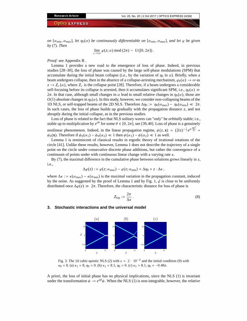
Fig. 3. The 1d cubic-quintic NLS (2) with ε = 2 · 10−2 and the initial condition (9) withκ0 = 8. (a) κ1 = 8, η0 = 0. (b) κ1 = 8.1, η0 = 0. (c) κ1 = 8.1, η0 ≈ −0.48π.

A priori, the loss of initial phase has no physical implications, since the NLS (1) is invariantunder the transformation ψ → eiβψ. When the NLS (1) is non-integrable, however, the relative


phase between two beams [16,17,30,42] or condensates [27] can have a dramatic effect on theirinteraction, thus making the loss of initial phase physically important. To illustrate that, consideragain the cubic-quintic NLS (2) for d = 1 with the two crossing beams initial condition

ψ0(x) = eiθxRκ0 (x − a) + eiη0 e−iθx Rκ1 (x + a) , (9)

where a = 12, θ = π8 , κ0 = 8, and Rκ is the solitary wave of (2). By Galilean invariance, before

the beams intersect at (zcross , xcross) ≈ (14.7, 0), each beam propagates as a solitary wave, andso

ψ(z, x) ≈ eiκ0zeiθx−iθ2z Rκ0 (x − a − 2θz)

+eiη0 eiκ1ze−iθx−iθ2z Rκ1 (x + a + 2θz) .

Hence, the difference between the on-axis phases of the two beams at (zcross , xcross) is

Δϕ ≈ (κ1 − κ0)zcross + η0 . (10)

When the two input beams are in-phase (η0 = 0) and identical (κ0 = κ1), they intersect in-phase (Δϕ = 0), and so they merge into a strong central beam, see Fig. 3(a). If we introducea 1.25% change in the propagation constant of the second beam (κ1 = κ0 + 0.1), then by (10),Δϕ ≈ 0.1 · 14.7 ≈ 0.48π. This phase difference is sufficient for the two beams to repel eachother, see Fig. 3(b). Therefore, the interaction is "chaotic", in the sense that a small change inthe input beams leads to a large change in the interaction pattern. To further demonstrate thatthe change in the interaction pattern is predominately due to the phase difference, we "correct"the initial phase of the second beam by setting η0 ≈ −0.48π, so that Δϕ ≈ 0 at (zcross , xcross),and indeed observe that the two beams merge, see Fig. 3(c). Unlike Fig. 3(a), the output beam isslightly tilted upward, since the lower input beam is more powerful, and therefore the net linearmomentum points upward.

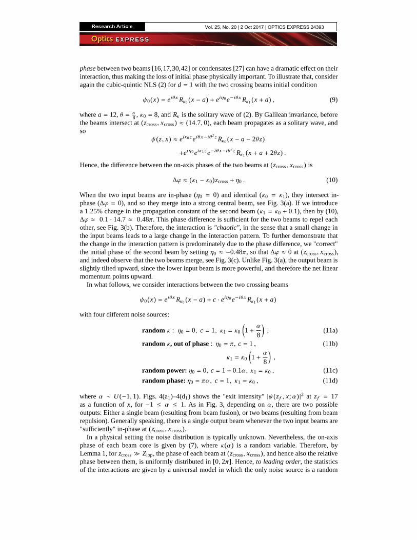
In what follows, we consider interactions between the two crossing beams

ψ0(x) = eiθxRκ0 (x − a) + c · eiη0 e−iθx Rκ1 (x + a)

with four different noise sources:

random κ : η0 = 0, c = 1, κ1 = κ0

(1 +

α

8

), (11a)

random κ, out of phase : η0 = π, c = 1 , (11b)

κ1 = κ0

(1 +

α

8

),

random power: η0 = 0, c = 1 + 0.1α, κ1 = κ0 , (11c)

random phase: η0 = πα, c = 1, κ1 = κ0 , (11d)

where α ∼ U (−1, 1). Figs. 4(a1)–4(d1) shows the "exit intensity" |ψ(z f , x; α) |2 at z f = 17as a function of x, for −1 ≤ α ≤ 1. As in Fig. 3, depending on α, there are two possibleoutputs: Either a single beam (resulting from beam fusion), or two beams (resulting from beamrepulsion). Generally speaking, there is a single output beam whenever the two input beams are"sufficiently" in-phase at (zcross , xcross).

In a physical setting the noise distribution is typically unknown. Nevertheless, the on-axisphase of each beam core is given by (7), where κ(α) is a random variable. Therefore, byLemma 1, for zcross � Zlop, the phase of each beam at (zcross , xcross), and hence also the relativephase between them, is uniformly distributed in [0, 2π]. Hence, to leading order, the statisticsof the interactions are given by a universal model in which the only noise source is a random


α

x

(a1)

−1 0 1

10

0

−10

α

(b1)

−1 0 1

10

0

−10

α

(c1)

−1 0 1

10

0

−10

α

(d1)

−1 0 1

10

0

−10

1 2

22%

78%

num. of beams

(c2)

1 2

24%

76%

num. of beams

(a2)

1 2

24%

76%

num. of beams

(d2)

1 2

21%

79%

num. of beams

(b2)

−6 −4 −2 0 2 4 6

| |

| |

| |

| |

| |

| |

| |

| |

| |

| |

| |

| |

x

(e)

(12a)

(12b)

(12c)

(12d)

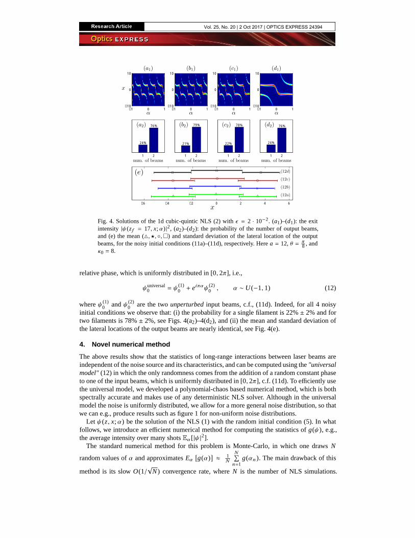
Fig. 4. Solutions of the 1d cubic-quintic NLS (2) with ε = 2 · 10−2. (a1)–(d1): the exitintensity |ψ(z f = 17, x; α) |2, (a2)–(d2): the probability of the number of output beams,and (e) the mean ( , �, ◦,�) and standard deviation of the lateral location of the outputbeams, for the noisy initial conditions (11a)–(11d), respectively. Here a = 12, θ = π

8 , andκ0 = 8.

relative phase, which is uniformly distributed in [0, 2π], i.e.,

ψuniversal0 = ψ (1)

0 + eiπαψ (2)0 , α ∼ U (−1, 1) (12)

where ψ (1)0 and ψ (2)

0 are the two unperturbed input beams, c.f., (11d). Indeed, for all 4 noisyinitial conditions we observe that: (i) the probability for a single filament is 22% ± 2% and fortwo filaments is 78% ± 2%, see Figs. 4(a2)–4(d2), and (ii) the mean and standard deviation ofthe lateral locations of the output beams are nearly identical, see Fig. 4(e).

4. Novel numerical method

The above results show that the statistics of long-range interactions between laser beams areindependent of the noise source and its characteristics, and can be computed using the "universalmodel" (12) in which the only randomness comes from the addition of a random constant phaseto one of the input beams, which is uniformly distributed in [0, 2π], c.f. (11d). To efficiently usethe universal model, we developed a polynomial-chaos based numerical method, which is bothspectrally accurate and makes use of any deterministic NLS solver. Although in the universalmodel the noise is uniformly distributed, we allow for a more general noise distribution, so thatwe can e.g., produce results such as figure 1 for non-uniform noise distributions.

Let ψ(z, x; α) be the solution of the NLS (1) with the random initial condition (5). In whatfollows, we introduce an efficient numerical method for computing the statistics of g(ψ), e.g.,the average intensity over many shots Eα[|ψ |2].

The standard numerical method for this problem is Monte-Carlo, in which one draws N

random values of α and approximates Eα[g(α)] ≈ 1

N

N∑n=1

g(αn ). The main drawback of this

method is its slow O(1/√

N ) convergence rate, where N is the number of NLS simulations.


If g(α) := g(ψ(·; α)) is smooth in α, however, we can use orthogonal polynomials as aspectrally accurate basis for interpolation [43] and numerical integration. Let α is distributedin [αmin , αmax] according to a PDF c(α), and let {pn (α)}∞n=0 be the corresponding sequence of

orthogonal polynomials, in the sense thatαmax∫

αmin

pn (α)pm (α)c(α) dα = δn ,m . For example, if α

is uniformly distributed in [−1, 1], then {pn } are the Legendre polynomials, and if α is normallydistributed in (−∞,∞), then {pn } are the Hermite polynomials. Recall that for smooth solutions

one has the spectrally accurate quadrature formula Eα[g(α)] ≈ N∑

j=1g(αN

j)wN

j, where {αN

j}Nj=1

and{wN

j

}Nj=1

are the roots of the orthogonal polynomial pN (α) and their respective weights

wNj=

αmax∫

αmin

N∏i=1, i� j

α−αNi

αNj −αN

i

c(α) dα. See [44] for a numerically efficient and stable algorithm

for computing the quadrature points and weights{αNj, wN

j

}Nj=1

. We apply the collocation

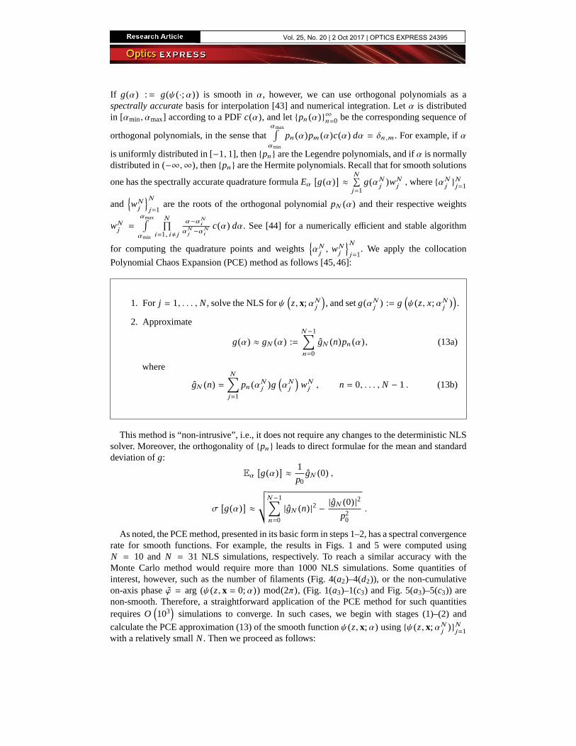
Polynomial Chaos Expansion (PCE) method as follows [45, 46]:

1. For j = 1, . . . , N , solve the NLS for ψ(z, x; αN

j

), and set g(αN

j) := g

(ψ(z, x; αN

j)).

2. Approximate

g(α) ≈ gN (α) :=N−1∑

n=0

gN (n)pn (α), (13a)

where

gN (n) =N∑

j=1

pn (αNj )g(αNj

)wN

j , n = 0, . . . , N − 1 . (13b)

This method is “non-intrusive”, i.e., it does not require any changes to the deterministic NLSsolver. Moreover, the orthogonality of {pn } leads to direct formulae for the mean and standarddeviation of g:

Eα[g(α)] ≈ 1

p0gN (0) ,

σ[g(α)] ≈√√√

N−1∑

n=0

|gN (n) |2 − |gN (0) |2p2

0

.

As noted, the PCE method, presented in its basic form in steps 1–2, has a spectral convergencerate for smooth functions. For example, the results in Figs. 1 and 5 were computed usingN = 10 and N = 31 NLS simulations, respectively. To reach a similar accuracy with theMonte Carlo method would require more than 1000 NLS simulations. Some quantities ofinterest, however, such as the number of filaments (Fig. 4(a2)–4(d2)), or the non-cumulativeon-axis phase ϕ = arg (ψ(z, x = 0; α)) mod(2π), (Fig. 1(a3)–1(c3) and Fig. 5(a3)–5(c3)) arenon-smooth. Therefore, a straightforward application of the PCE method for such quantitiesrequires O

(103)

simulations to converge. In such cases, we begin with stages (1)–(2) and

calculate the PCE approximation (13) of the smooth function ψ(z, x; α) using {ψ(z, x; αNj

)}Nj=1

with a relatively small N . Then we proceed as follows:


3. Use the gPC interpolant (13) to obtain ψ(·, αm ) ≈ ψN (·, αm ) on a sufficiently densegrid {αm }Mm=1, where M � N .

4. Compute g(αm ) ≈ g(ψN (·, αm )) for m = 1, . . . , M ,

5. Compute the statistics of g(ψ) using {g(ψN (·, αm ))}Mm=1.

For example, when we computed the number of beams at z = z f in Fig. 4, we firstcomputed the PCE interpolant ψN (z f , x; α) with N = 71. Then we computed ψ(z f , x; αm ) ≈ψN (z f , x; αm ) for m = 1, . . . , M = 801. For each αm , we count the number of filaments andused this to produce the histogram in figure 4(a2)–4(d2). The additional computational cost ofsampling ψN (13) at M � N grid points in step (3) is negligible compared to directly solvingthe NLS for N times in stage (1).

5. Conclusions

In this study, we showed that when two (or more) laser beams interact after a sufficientlylong propagation distance, their relative phase at the crossing point varies so much fromshot to shot, that the outcome of their interaction cannot be deterministically predicted orcontrolled. In such cases, the notion of a "typical experiment" or a "typical solution" may bemisleading, and one should adopt a stochastic approach. The loss of phase can explain someof the difficulties in phase-dependent methods in optical communications such as QuadratureAmplitude Modulation (QAM) [2], and in coherent combining of hundreds of laser beamsin a small space for ignition of nuclear fusion [15], and for creating a more powerful laserbeam [6]. In these applications, controlling the phases of the input beams or pulses might notprovide a good control over their interaction or combination, due to the loss of phase. Our studysuggests that controlling the relative phases at the intersection point may be achieved by eithershortening the propagation distance, or by coupling the beams throughout the propagation. Lossof phase can also explain the high sensitivity to initial perturbations of interactions betweentopologically-charged solitons [47]. Loss of phase is also relevant to the loss of polarization forelliptically-polarized beams [48].

Appendix

A. Loss of phase in two dimensions

We repeated the simulations of Fig. 1 in two dimensions, see Fig. 5. As in the one-dimensionalcase, the phase variation increases with the propagation distance, and becomes uniformly dis-tributed around z = 2, see Fig. 5(c3).

To compare the rates at which the PDFs of ϕ converge to the uniform distribution funi(y) :≡1

2π on [0, 2π], we plot in Fig. 6(a) the distance ‖ f − funi‖ :=2π∫

0

∣∣∣ f (y) − 12π

∣∣∣ dy. Note that the

convergence is not monotone, because the distance has a local minimum whenever Δϕ = 2πkfor an integer k.

The convergence is much faster for d = 2 than for d = 1. This is because typically, Δκ ismuch larger in 2d than in 1d. For example, in Fig. 6(b) Δκ ≈ 25 in 2d, and Δκ ≈ 1.8 in 1d.Intuitively, this is because the input beam evolves into a solitary wave, and over a given powerrange, the propagation constant of the solitary wave changes considerably less in 1d than in2d. Hence, by (8), the loss of phase occurs much faster in the two-dimensional case than in theone-dimensional case, thus explaining Fig. 6(a).


−1 10

40z = 0.2

ϕ

α

(a1)

−1 115

55z = 1

α

(b1)

−1 140

80z = 2

α

(c1)

−1 10

2π

α

ϕ(a2)

−1 10

2π

α

(b2)

−1 10

2π

α

(c2)

0 2πϕ

f132π

0

(a3)

0 2πϕ

12π

0

(b3)

0 2πϕ

12π

0

(c3)

0 20

15

|x|

|ψ|(a4)

0 20

15

|x|

(b4)

0 20

15

|x|

(c4)

Fig. 5. Same as figure 1 for d = 2.

0 5 10 150

2

z

‖f−f u

ni‖

(a)

−1 10

50

α

κ

(b)

Fig. 6. The cubic-quintic NLS (2) with ε = 10−3, and the initial condition (5) in one (dot-dash) and two (solid) dimensions. (a) Distance between the PDF of ϕ and the uniformdistribution on [0, 2π] . (b) The propagation constant of the beam core, see (6), as a functionof α.

The reason why Δκ is much larger in 2d than in 1d is as follows: denote the solitary-wavepower by P(κ) :=

∫ |Rκ |2 dx. When ε = 0 in (2), then dPdκ = 0 for d = 2 but dP

dκ > 0 ford = 1 [33]. Hence, if 0 < ε 1, then dP

dκ = O(ε ) for d = 2, but dPdκ = O(1) for d = 1.

Therefore dκdP= O(1) for d = 1 but dκ

dP= O( 1

ε ) for d = 2.

B. Proof of Lemma 1

For a given z ≥ 0, denote ϕz (α) = κ(α) + η0 (α)z

, then ϕ(α) = zϕz (α) mod (2π). We prove thatlimz→∞ ϕ(α) ∼ U ([0, 2π]) by showing that for every 0 ≤ a < b ≤ 2π,

limz→∞ μ

(ϕ−1 ([a, b])

)=

b − a2π

, (14)

where ϕ [a, b] := {α ∈ [αmin , αmax] | uz (α) ∈ [a, b]}.We first prove the lemma for a strictly monotone function κ on (αmin , αmax). For sufficiently


large z, ϕz is also monotone. Let xzk

and yzk

be the solutions of

ϕz (xzk) =

2kπ + az

, ϕz (yzk) =

2kπ + bz

, k ∈ Z . (15)

There exists kmin ≤ kmax such that xzkmin−1 and yz

kmax+1 do not exist, and for clarity wesuppressed the dependence of kmin and kmax on z. By definition,

μ(ϕ−1 ([a, b])

)=

kmax∑

k=kmin

μ(xzk, yz

k

)+ E(z) =

=

kmax∑

k=kmin

μ

(ϕ−1z

(2πk + a

z

), ϕ−1

z

(2πk + b

z

))+ E(z) , (16)

where the error term E(z) exists if either yzkmin−1 > αmin or xz

kmax+1 < αmax exist. In such cases,since dμ is continuous,

E(z) = μ([αmin , y

zkmin−1]

)+ μ([xz

kmax+1 , αmax]).

We now show that if yzkmin−1 exists, then lim

z→∞ μ(αmin , y

zkmin−1

)= 0 (a similar proof holds

also for xzkmax+1). It is enough to show that lim

z→∞ xzkmin= αmin, because yz

kmin −1< xkmin and μ is a

continuous measure. Let δ > 0, then

zϕz (αmin + δ) − zϕz (αmin) =

(η0(αmin + δ) − η0(αmin)) + z (κ(αmin + δ) − κmin)

goes to infinity as z → ∞. Therefore, for large enough z, xzkmin∈ (αmin , αmin + δ). Thus, for all

δ > 0,αmin ≤ lim

z→∞ xzkmin

< αmin + δ .

Since ϕz is strictly monotone, then by the inverse function theorem ϕ−1z ∈ C1, and so by

substituting α = ϕ−1z (y),

μ

(ϕ−1z

(2πk + a

z

), ϕ−1

z

(2πk + b

z

))=

ϕ−1z

(2πk+b

z

)∫

ϕ−1z

(2πk+a

z

)c(α) dα =

2πk+bz∫

2πk+az

gz (y) dy ,

where gz (y) := c(ϕ−1z (y))(ϕ−1

z )′(y). By Lagrange mean-value theorem, for each index k, thereexists ξz

k∈ (a, b) such that

μ

(ϕ−1z

(2πk + a

z

), ϕ−1

z

(2πk + b

z

))=

gz

(2πk + ξz

k

z

)b − a

z.


Substituting the above into (16) yields

μ(ϕ−1z ([a, b])

)=

b − az

kmax∑

k=kmin

gz

(2πk + ξz

k

z

)+ E(z) . (17)

Next, consider the integrals

I :=

αmax∫

αmin

c (α) dy = μ (αmin , αmax) = 1 , (18a)

I2 :=

yzkmax∫

xzkmin

c(α) dα =

2πkmax+bz∫

2πkmin+az

gz (y) dy .

Using Riemann sums

I2 =2πz

kmax∑

k=kmin

gz

(2πk + ξz

k

z

)+O(z−1). (18b)

Denoting ϕz (αmin) := ϕz ,min and ϕz (αmax) := ϕz ,max Since

ϕz ,max∫

ϕz ,min

=

ϕz (xzkmin

)∫

ϕz ,min

+

ϕz (y zkmax

)∫

ϕz (xzkmin

)

+

ϕz ,max∫

ϕz (y zkmax

)

,

then I = I2 +O(z−1). Equating (18b) and (18a), and substituting into (17), yields

μ(ϕ−1z ([a, b])

)=

b − a2π+ o(1) ,

by which we prove (14)Finally, if κ, hence ϕz is piece-wise monotone, we apply the above proof for each sub-interval

over which ϕz is monotone, and by additivity of measure have the result.

Funding

The research of AS and GF was partially supported by grant #177/13 from the Israel ScienceFoundation (ISF).

Acknowledgment

We thank B.A. Malomed and A.L. Gaeta for useful discussions.


loss of phase and universality of stochastic interactions ...fibich/manuscripts/lop-oe17.pdf ·...

Documents