University of LjubljanaFaculty of Mathematics and Physics

department of physics

Lifshitz interactions and stochastic electrodynamics

Third Year Seminar

Student: Giovanni BanelliMentor: prof. Rudolf Podgornik

Ljubljana, March 2016

Abstract

Evgenii Lifshitz’s solution of the various Casimir problems is presented, with afocus on Rytov’s theory of thermal fluctuations of the zero-point field, upon whichLifshitz’s calculation is based. We start with a historical review of the reasons thatled to the formulation of the problem of zero-point field, from Planck’s solution ofthe black body issue to van der Waals’s discovery of anomalous interactions betweenmolecules. Finally an explanation of this approach is outlined in light of its impor-tance for the birth of the alternative theory of stochastic electrodynamics, brieflyindicating its effectivenesses and difficulties.

The seminar is written without any reference to quantum field theory and thus issuitable for Bachelor students to help them understand the problem of the interplayof microscopic and macroscopic worlds in electromagnetic field theory.

Contents1 Prologue 2

1.1 The discovery of the quantum nature of light . . . . . . . . . . . . . 21.2 Quantum electrodynamics . . . . . . . . . . . . . . . . . . . . . . . . 3

2 Casimir’s problem 42.1 Van der Waals microscopic forces . . . . . . . . . . . . . . . . . . . . 42.2 Casimir’s macroscopic computation . . . . . . . . . . . . . . . . . . . 4

3 Lifshitz’s solution 63.1 Macroscopic approach . . . . . . . . . . . . . . . . . . . . . . . . . . 63.2 Rytov’s theory . . . . . . . . . . . . . . . . . . . . . . . . . . . . . . 63.3 Calculation . . . . . . . . . . . . . . . . . . . . . . . . . . . . . . . . 73.4 Remarks . . . . . . . . . . . . . . . . . . . . . . . . . . . . . . . . . . 12

4 Epilogue. Stochastic electrodynamics 13

1

1 Prologue

1.1 The discovery of the quantum nature of lightIt’s a shared opinion among scholars that the beginning of the quantum era is

marked by the discovery of the correct blackbody spectrum. In 1900 Planck1 wasthe first able to derive a formula which gives as limiting cases the previously knownand experimentally verified Rayleigh-Jeans2 and Wien3 formulas. His derivation wasmade by means of classical statistical theory applied to thermodynamics and, drivenby the aim to get the desired result, he was forced to use a mathematical expedientthat later revealed completely new physics behind it.

In particular, given the classical oscillator model of an atom, by equalizing theabsorption and emission rates obtained in this way[1], he got an equation for thefrequency dependent oscillator energy density ρ(ω) (where we have the overall energyof the system of oscillators defined as E =

∫ ωmax0 ρ(ω)dω):

ρ(ω) =ω2

π2c3U(ω), (1)

where U(ω) is the total energy of the oscillator. In computing the latter, he assumedthat a system of oscillators had an overall energy ofNU = Pε, where P is the numberof the discrete amounts of energy ε the total is made of. Then by computing theentropy of the P-N system (according to Boltzmann4 this is S = kB logW where Wis the number of ways in which the P energy elements can be distributed among theN radiators)[1] he came to the result

U(ω, T ) = ε · 1

eε

kBT − 1= ~ω · 1

e~ωkBT − 1

, (2)

where the value for ε was established because it describes very well the final distri-bution obtained putting (2) in (1) (Planck’s law).

We remark here that this is the first time in history when the "quantum" conceptis used. Additionally, in the computation of entropy, it was crucial to considerthe discrete amounts of energy as indistinguishable, thus introducing one of themain axioms of the quantum theory. The idea of the photon was later confirmedby Einstein with his photoelectric effect explanation. Now we know that the twoformulae above are correct because we can compute them from statistical theory ina simpler fashion if we assume the quantum concept: the coefficient in equation (1)is the photon 3D density of states (remember to consider that the photon has twopolarizations), while the second function in the product (2) is the Bose-Einstein5

distribution which is valid for photons.However the ρ(ω) we have still isn’t correct. If we take the limit kBT � ~ω we

get

U =~ω

e~ωkBT − 1

w~ω

1 + ~ωkBT

+ 12( ~ωkBT

)2 − 1=

kBT

1 + 12

~ωkBT

w kBT −1

2~ω (3)

1Max Planck (1858-1947), German theoretical physicist2John Rayleigh (1842-1919), English physicist; James Jeans (1877-1946), English physicist, astronomer

and mathematician3Wilhelm Wien (1864-1928), German physicist4Ludwig Boltzmann (1844-1906), Austrian physicist and philosopher5Satyendra Nath Bose (1894-1974), Indian physicist; Albert Einstein (1879-1955), German-born the-

oretical physicist

2

i.e. a first order correction to the classical limit. This means that in order to havea clean equipartition theorem result for high temperatures we need to add a 1

2~ωterm. The present work wishes to discuss about the nature of this term focusing onan unusual interpretation of it.

1.2 Quantum electrodynamicsWhen he wrote his first blackbody theory, Planck was aware of this and tried

to find another way to derive the expression that included the missing part, stillwithin the domain of statistical thermodynamics. After some time he succeededin this, however, the physical significance of some mathematical assumptions hadalready marked this "second theory" as unlikely to correspond to truth (for instancehe postulated that absorption proceeded in the classical fashion, while emission wascomposed of the outgoing quanta[1]).

Anyway, some years later, the formal development of quantum formalism allowedto compute the Planck spectrum from this perspective and showed that the originalresult by Planck together with the constant correction yielded the exact result forblackbody emission energy density, which finally turns out to be

ρ(ω, T ) =~ω3

π2c3

(1

e~ωkBT − 1

+1

2

). (4)

So which is the correct way to interpretate Planck’s result? Actually only the firstterm in the sum is referring directly to matter, i.e. to the emitting body, while thesecond term indicates that at the same time we have another amount of energy whichis contributing to the spectrum. In particular, if we put temperature to be zero, westill have a nonzero spectrum. This spectrum is due to the so-called zero-pointenergy (the energy of the ground/zero state of the oscillators). It’s important hereto remark, that the first Planck’s calculation, the formally consistent one, couldn’taccount for this term in the limiting case of T=0; but the same calculation in theopposite limit (T =∞) suggested the need to add it.

In other words, we can say that a classical attempt to explain emission andabsorption of electromagnetic radiation of bodies over the whole temperature scalewithout taking into account collateral phenomena is impossible, and that the solefact of using some quantum assumptions in the derivation (i.e. the quantizationof energy) shows automatically where this interpretation is lacking, this is in thepresence of a zero-point field responsible for the above mentioned zero-point energy(we call this field that way in analogy with the given definition of zero-point energy).This zero-point field in fact is showing to have a quantum nature, and in modernquantum electrodynamics has its own role. However, not being able at this pointto explain everything in those terms, we shall see that another interpretation of thezero-point energy is possible, because it can give the same calculation results whenapplied to some concrete physical problems which are experimentally verifiable.

3

2 Casimir’s problem

2.1 Van der Waals microscopic forcesIn 1873 van der Waals6 reformulated the ideal gas law in order to take into ac-

count the intermolecular forces that were influencing gas under certain conditions.During the next years these forces were found out to be consequence of permanent(Keesom7) or induced (Debye8) dipoles on molecules. However, it immediately be-came clear that there must be another contribution to match experimental data,and that this contribution might be found in terms of the just born quantum theory.The problem was finally resolved in 1930 by London9, who employing fourth-orderquantum mechanical perturbation theory derived an attraction potential betweenpolarizable molecules inversely proportional to the sixth power of their distance(∝ R−6). This theory was then further perfectioned by the work of Casimir10 andPolder11, who proposed that for large distances the potential of attraction shouldfall even faster (∝ R−7) because of taking into account retardation effects.

Once this "elementary" problem had been solved, the question of the generaliza-tion of this theory for macrostructures was set. Casimir and Polder first calculated,still by means of quantum field theory, the interaction between an atom (molecule)and a perfectly conducting wall, simplifying the problem to the interaction of thatatom with its image on the surface. Next a further generalization had to be done,trying to evaluate the force between two perfectly conducting plates. Such a stepwould have a great importance since it could give predictions that might be experi-mentally confirmed.

2.2 Casimir’s macroscopic computationThe problem above was first tackled independently by Casimir in 1948. At the

beginning he understood that an alternative approach to the perturbative methodcould be used in this case. He referred directly to the concept of zero-point energy,and calculated the difference between the amounts of energy of the considered system(due to the ground state of the electromagnetic vacuum) when the plates are close

6Johannes Diderik van der Waals (1837-1923), Dutch theoretical physicist7Willem Hendrik Keesom (1876-1956), Dutch physicist8Peter Debye (1884-1966), Dutch-born physicist and physical chemist9Fritz London (1900-1954), German-born physicist

10Hendrik Casimir (1909-2000), Dutch physicist11Dirk Polder (1919-2001), Dutch physicist

4

to each other at a distance of ` and when they are far apart, given that for a singlefrequency this energy is

Ei =1

2~ωi. (5)

In two directions of the space (y and z) all frequencies are available, while in thechosen x direction for a finite separation the modes are discrete:

kx =π

`n. (6)

We shall therefore integrate over the formers and sum up the latter ones:

∆E = 21

2~c(

L

π)2[∑′

n

∫ ∞0

dky

∫ ∞0

dkz((π

`n)2 + k2y + k2z)

12

−dπ

∫ ∞0

dkx

∫ ∞0

dky

∫ ∞0

dkz(k2x + k2y + k2z)

12 ],

(7)

where L2 is the area of the plates. Note that each state has two polarizations, exceptwhen n=0 (for this reason there’s a prime on the summation symbol).

Both parts of this expression are of course an infinite quantity, however it ispossible to show that their difference is finite[1].

Deriving with respect to ` the result divided by L2 gives the attractive force Fper unit area between the plates:

F =1

L2

d∆E

d`=

π2

240

~c`4. (8)

However that’s not enough: the idealization of perfect conductivity, which deter-mined the discrete values in the above calculation (on the surface there are nocharges so the tangential components of the field have to be zero) is too far fromreality. In order to consider this model for experimental validation it is necessary toinclude an approximation that should account for the properties of matter, i.e. forits polarizability.

Hamaker12 suggested obtaining the interaction between macroscopic bodies ina pairwise summation over molecules inside both plates, according to the Casimir-Polder model of the interaction of molecules facing themselves through a conductingmirror. Unfortunately experiment gave evidence for much a stronger interactionbetween the plates than what was predicted in this way[1]. This confirmed thehypothesis that in non-rarefied media van der Waals forces cannot be accounted forin a linear pairwise approximation. Consequently the calculation of the overall forcebetween dielectric bodies had to be performed inside the zero-point field framework,this is the framework already used by Casimir in the case of conductors. Then,if such a calculation proved to be true, Van der Waals forces would look to arisedirectly from the zero-point field, and from its energy variations due to the presenceof (polarizable) bodies.

12Hugo Christiaan Hamaker (1905-1993), Dutch scientist

5

3 Lifshitz’s solution

3.1 Macroscopic approachPerhaps because of its complexity, a QED computation of the interaction forces

between real (dielectric) macroscopic bodies caused by their microscopic componentshad taken a long time (Kampen-Nijboer-Schram, 1968) to be performed. As alluded,however, surprisingly this was made possible much earlier by the work of Lifshitz13

(1955)[2]. The most interesting feature of his theory is that it’s performed on anapparently pure classical basis, and correctly anticipated all the later QED resultson this topic.

This Lifshitz’s theory is in fact "classical" first of all beacuse it approaches theproblem considering the bodies as macroscopic structures characterized by the pa-rameters of matter that are used in Maxwellian14 formulation of electrodynamics,this is notably the complex dielectric constant ε = ε(ω). Provided that at thequantum scale close to the absolute zero there is a non vanishing energy field (assuggested by Planck) and that this field itself is responsible for attraction forcesbetween bodies (as predicted by Casimir), it was unavoidable that an alternativetheoretical picture of the problem should account for this field, too.

3.2 Rytov’s theoryWhat is today commonly referred to as the Lifshitz theory of zero-point field

interactions (from this the denomination "Lifshitz interactions") originates fromthe arguments written by Lifshitz in his article[2] used to deal with the Casimir’sproblem. Actually, like Lifshitz himself wrote in the introduction, his calculationsstem from the application of the general theory of electromagnetic field fluctuationsdiscussed by Rytov15 in his monograph[3]. In this work published a few years before(1953) Rytov makes an extension of Maxwellian macroscopic electrodynamics withclassical physical-statistical methods, primarly to explain the origin of electrical noisein circuits by means of thermal radiation "in the form of a unified theory" (thesewords marking his advance compared to Nyquist’s16 work on the same topic).

The main innovative argument of Rytov’s research is to consider that during theprocess of absorption of light (note: always classically speaking) at least a part ofgained energy goes back to vacuum, where macroscopic matter "floats". Because ofthis, energy is deposited into the fluctuating field in vacuo. In this way we considerthe fluctuating field in the same way as fluctuation is defined in statistical physics;this means that the field has a random value over time, but when time averaged itis reduced to zero. This field, which Rytov in his work calls "chaotic lateral field",- directly citing:

distributed over the volume of the bodies under consideration consti-tutes the basis for the application of statistics to general electrodynamics.The action of this field determines the fluctuation of the charge and ofthe current in bodies, and thereby also the corresponding fluctuation ra-diation (i.e. electrical noise, ed.).

13Evgenii Mikhailovich Lifshitz (1915–1985), Soviet physicist14James Clerk Maxwell (1831-1879), Scottish theoretical physicist15Sergei Mikhailovich Rytov (1908-1996), Soviet physicist16Harry Nyquist (1889-1976), Swedish-born electronic engineer

6

We remark from the quotation that the field is called "lateral" because it is a collat-eral phenomenon to the presence inside vacuum of matter which is absorbing light.It is attributed to vacuum but it cannot exist in vacuum alone.

The result of this idea is that to solve Maxwell equations they have to be properlyamended, to account for the presence of a field that is not caused by real charges orcurrents:

ε(ω)ε0∇ ·E = ρ, ∇ ·B = 0, (9)

∇×E = −∂B∂t, ∇×H = j + ε(ω)ε0

∂E∂t

+∂K∂t

. (10)

Here ε(ω) = ε′(ω)+iε′′(ω) is the complex dielectric constant and K is a random fielddescribing the polarization fluctuations (for a nonmagnetic medium we set µ = 1).

Another fundamental step made by Rytov in his work is to define a necessaryproperty of the fluctuating field to allow further calculation. Given that the field isstochastic in time, its space correlation function is given by:

< Ki(x, y, z, t)Kj(x′, y′, z′, t′) >= Aε′′(ω)ε0δijδ(x− x′)δ(y − y′)δ(z − z′)δ(t− t′),

(11)

A = 4~

(1

e~ωkBT − 1

+1

2

).

This is the average value of the product of components (i, j) ∈ (x, y, z) of the field attwo different points in space; we see that the field is in this respect homogenous be-cause of our macroscopic assumptions. A more compact notation for this is possibleif we consider that

2

(1

ex + 12

)= coth

x

2(12)

(later we will use this form). Rytov’s derivation of this formula is quite long andcomplex, but for us it is enough to note that it includes the same temperaturedependence of Planck’s law. It is interesting that the fluctuating field, though beingnot properly a body made of oscillators which re-emits absorbed light, must besuch as to include the zero-point field contribution and the "matter" contribution(remember, the fluctuating field is regarded as external to matter, and for thisreason is said to belong to vacuum, but at the same time it cannot exist withoutthe presence of matter). Furthermore it is relevant that, as expected, the formulaincludes as an indispensable factor the imaginary part of the dielectric constant, thepart responsible for absorption; absorption itself namely implies the existence of thefluctuating field.

What Rytov had just derived is in fact what today we call the "fluctuation-dissipation theorem" (where dissipation is a synonym for absorption). This is ageneral physical-statistical tool that had already been used by Nyquist (to explainJohnson17 noise), but it got a rigorous formulation only much later with Kubo18

(1967).

3.3 CalculationLet’s go back to our problem and follow Lifshitz’s solution. The system is made

of just two infinite plates, so there are no free charges and currents (ρ = 0 and j = 0).17John Bertrand Johnson (1887-1970), Swedish-born electrical engineer and physicist18Ryogo Kubo (1920-1995), Japanese mathematical physicist

7

We solve it for monochromatic fields with time factor e−iωt. For an easier calculationwe rewrite so obtained Maxwell equations in Gauss19 notation (H ≡

√4πµ0H,

E ≡√

4πε0E):

∇ ·E = 0, ∇ ·H = 0, (13)

∇×E = iω

cH, ∇×H = −iε(ω)

ω

cE− iω

cK. (14)

These are the equations for the electric field E and magnetic field H that differ fromthe ordinary empty space Maxwell equations becasue of the presence of stochasticsources proportional to the time derivative of K. The first two just require, as usualin vacuum, that the fields must be transversal to the waves ((24) and (28)), sowe actually have a set of two partial differential vector equations for two vectorunknowns; we try to find solutions in the form of Fourier20 integrals. Since we canexpress also the random field K in terms of its known Fourier components g(k) (sothat K(r) =

∫∞−∞ g(k)eikrdk), we get

< gi(k)gj(k′) >=1

4π3Aε′′(ω)δijδ(k − k′). (15)

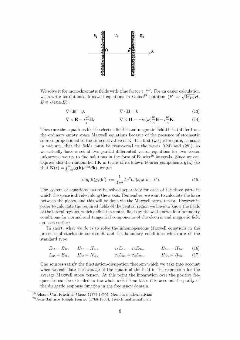
The system of equations has to be solved separately for each of the three parts inwhich the space is divided along the x axis. Remember, we want to calculate the forcebetween the plates, and this will be done via the Maxwell stress tensor. However inorder to calculate the required fields of the central region we have to know the fieldsof the lateral regions, which define the central fields by the well-known four boundaryconditions for normal and tangential components of the electric and magnetic fieldon each surface.

In short, what we do is to solve the inhomogeneous Maxwell equations in thepresence of stochastic sources K and the boundary conditions which are of thestandard type

E1t = E3t, H1t = H3t, ε1E1n = ε3E3n, H1n = H3n; (16)E3t = E2t, H3t = H2t, ε3E3n = ε2E2n, H3n = H2n. (17)

The sources satisfy the fluctuation-dissipation theorem which we take into accountwhen we calculate the average of the square of the field in the expression for theaverage Maxwell stress tensor. At this point the integration over the positive fre-quencies can be extended to the whole axis if one takes into account the parity ofthe dielectric response function in the frequency domain.

19Johann Carl Friedrich Gauss (1777-1855), German mathematician20Jean-Baptiste Joseph Fourier (1768-1830), French mathematician

8

To show how all this works we perform calculations for the first part (with index1, i.e. for the medium with ε1). There the random field K takes the form of

K1(x, y, z) =

∫ ∞−∞

g(k)eiqr cos(kxx)dk (18)

where we have defined q = (0, ky, kz) and r = (0, y, z). This is an elementary Fouriertransform definition. Similarly we write the solutions for fields E1 and H1 in thefirst medium (note n = (1, 0, 0)):

E1 =

∫ ∞−∞{a1(k) cos(kxx) + ib1(k) sin(kxx)}eiqrdk +

∫ ∞−∞

u1(q)eiqr−is1xdq, (19)

H1 =c

ω

∫ ∞−∞{(q× a1 + kxn× b1) cos(kxx) + i(q× b1 + kxn× a1) sin(kxx)}eiqrdk

+c

ω

∫ ∞−∞

(q× u1 − s1n× u1)eiqr−is1xdq

(20)

with

s1 =

√ω2

c2ε1 − q2, (21)

where the first term is the solution of the inhomogeneous equations and the secondof the homogeneous (i.e. for K=0). The coefficients of the inhomogeneous equationare calculated from the second of the two considered Maxwell equations (rotH) whenwe define K as (18):

a1 =1

ε1(k2 − ω2

c2ε1)

[ω2

c2ε1g1 − q(qg1r)− k2xg1xn

], (22)

b1 =kx

ε1(k2 − ω2

c2ε1)

[n(qg1r) + qg1x] . (23)

Finally transversality condition (∇ ·E = 0) sets

u1rq− u1xs1 = 0. (24)

In the central part (with index 3, i.e. vacuum-no matter) for K=0 we have onlyhomogeneous solutions:

E3 =

∫ ∞−∞{v(q)eipx + w(q)e−ipx}eiqrdq, (25)

H3 =c

ω

∫ ∞−∞{(q× v + pn× v)eipx + (q×w − pn×w)e−ipx}eiqrdq (26)

with

p =

√ω2

c2− q2 (27)

and transversality conditions

vrq + vxp = 0, wrq− wxp = 0. (28)

Next we consider the boundary conditions, given that ε3 = 1:

E1t = E3t, H1t = H3t, ε1E1n = E3n, H1n = H3n. (29)

9

The missing equations for calculating all field Fourier amplitudes are found by solvingthe same problem on the other plate i.e. at x = `. There the formulation is the samewith appropriate indices, except for setting kx(x− `) in the arguments of harmonicfunctions instead of kxx. Solving the whole set of equations gives formulas for centralfields amplitudes in terms of the amplitudes g of the random field.

Now we can calculate the xx component of Maxwell stress tensor, perpendicularto the surfaces, by integrating over all frequencies (positive and negative); since theintegrated function is even, we get:

Fxx = 2

∫ ∞0

Fωdω =1

4π2

∫ ∞0

(E23x −

1

2E2

3 +H23x −

1

2H2

3 )dω

=1

4π

∫ ∞0

(E23r − E2

3x +H23r −H2

3x)dω.

(30)

The fields appearing above are intended to be statistically averaged (< Fxx >= ...).Note that the squares of both E and H contain double integrals over k and a seriesof products of g components whose result is given by (15) carrying out one of theseintegrations. In this regard remember that quantities g referring to different mediaare statistically independent, too, so their product is 0.

Next we perform separately another integration over dkx and substitute the in-tegration over dq with dp. The whole expression has to be simplified, neglecting theterms appearing without `-dependence, which are not relevant for the problem. Ifwe make the p variable dimensionless dividing it by ω

c the final result is obtained as:

< Fxx >≡ F =~

2π2c3

∫ ∞0

coth~ω

2kBTω3dω

∫p2dp{

[(s1 + p)(s2 + p)

(s1 − p)(s2 − p)e−2ipl

ωc − 1

]−1+

[(s1 + ε1p)(s2 + ε2p)

(s1 − ε1p)(s2 − ε2p)e−2ipl

ωc − 1

]−1}

(31)

with

s1 =√ε1(ω)− 1 + p2, s2 =

√ε2(ω)− 1 + p2 (32)

for

p =

√1− c2

ω2q2 (33)

defined on the real segment [0,1] and the whole upper half of the imaginary axis.The force between the plates would be the real part of this complicated analiticintegral.

However is possible to compute this integral in an easier way. If we do thetransformation ω = iξ we redefine the domain of p (33) over only real values from1 to infinity and we make the exponents in (31) real. Straightforwardly we see thateven the integration by ξ over the same domain as ω gives a real result. In fact wenote that the function coth ~ω

2kBThas an infinite number of poles on the imaginary

axis atωn = iξn = i

2T

~πn. (34)

The standard procedure that we use for evaluating this integral, taken from thetheory of analytic functions, is to first extend the integration domain of ξ to theupper right quadrant of the complex plane and then use the Cauchy theorem when

10

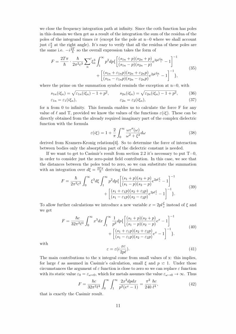
we close the frequency integration path at infinity. Since the coth function has polesin this domain we then get as a result of the integration the sum of the residua of thepoles of the integrand times iπ (except for the pole at n=0 where we shall accountjust iπ2 at the right angle). It’s easy to verify that all the residua of these poles arethe same i.e. −i2T~ so the overall expression takes the form of

F =2Tπ

~· ~

2π2c3

∑′

n

ξ3n

∫ ∞1

p2dp{[

(s1n + p)(s2n + p)

(s1n − p)(s2n − p)e2pl

ξnc − 1

]−1+

[(s1n + ε1np)(s2n + ε2np)

(s1n − ε1np)(s2n − ε2np)e2pl

ξnc − 1

]−1},

(35)

where the prime on the summation symbol reminds the exception at n=0, with

s1n(iξn) =√ε1n(iξn)− 1 + p2, s2n(iξn) =

√ε2n(iξn)− 1 + p2, (36)

ε1n = ε1(iξn), ε2n = ε2(iξn), (37)

for n from 0 to infinity. This formula enables us to calculate the force F for anyvalue of ` and T, provided we know the values of the functions ε(iξ). These can bedirectly obtained from the already required imaginary part of the complex dielectricfunction with the formula

ε(iξ) = 1 +2

π

∫ ∞0

ωε′′(ω)

ω2 + ξ2dω (38)

derived from Kramers-Kronig relations[4]. So to determine the force of interactionbetween bodies only the absorption part of the dielectric constant is needed.

If we want to get to Casimir’s result from section 2.2 it’s necessary to put T=0,in order to consider just the zero-point field contribution. In this case, we see thatthe distances between the poles tend to zero, so we can substitute the summationwith an integration over dξ = 2Tπ

~ deriving the formula

F =~

2π2c3

∫ ∞0

ξ3dξ

∫ ∞1

p2dp{[

(s1 + p)(s2 + p)

(s1 − p)(s2 − p)e2pl

ξc − 1

]−1+

[(s1 + ε1p)(s2 + ε2p)

(s1 − ε1p)(s2 − ε2p)e2pl

ξc − 1

]−1}.

(39)

To allow further calculations we introduce a new variable x = 2pl ξc instead of ξ andwe get

F =~c

32π2`4

∫ ∞0

x3dx

∫ ∞1

1

p2dp{[

(s1 + p)(s2 + p)

(s1 − p)(s2 − p)ex − 1

]−1+

[(s1 + ε1p)(s2 + ε2p)

(s1 − ε1p)(s2 − ε2p)ex − 1

]−1}.

(40)

withε = ε(i

xc

2p`). (41)

The main contributions to the x integral come from small values of x: this implies,for large ` as assumed in Casimir’s calculation, small ξ and p w 1. Under thosecircumstances the argument of ε function is close to zero so we can replace ε functionwith its static value ε0 = εω=0, which for metals assumes the value εω→0 →∞. Thus

F =~c

32π2`4

∫ ∞0

∫ ∞1

2x3dpdx

p2(ex − 1)=

π2

240

~c`4, (42)

that is exactly the Casimir result.

11

3.4 RemarksWe have at last obtained the same result as in (8). But how close may our

plates stand for, Casimir’s perfect metal approximation to remain still valid? Toanswer to such a question we need to compute the next term in the expansion ofour formula, and require it to be much smaller than the first term. This can bedone by replacing the limit ε = ∞ with its proper frequency dependence in thesurroundings. Lifshitz found out that the exact metal equation ε(ω) = 1 + iσ

ε0ω[4]

gives a very tiny correction, so for this purpose he had to take the plasma limitfor metals ε(ω) = 1 − e2N

ε0mω2 [4] (where unity can be neglected for low frequencies),which, for typical metal (e.g. silver) free-electron density N, requested the distanceto be much greater than 0.6µm. Similarly, for temperatures close to zero he used theexpansion of the integral over ξ in (39) towards summation of discrete frequencies in(35), given by the Euler sum formula, to discover that this limit is allowed whenever` � ~c

kBT. Surprisingly, in the case of silver, as long as ` < 5µm (but still well over

0.6µm) we can regard it as a perfect metal with T=0 even at room temperature[2].As Lifshitz points out in his article, Casimir in his computation couldn’t account

for all this. In fact equation (35) for the geometry of this problem (and the methodhere explained for any other one) has full generality and can be used to investigate alllimiting cases in both distance and temperature for bodies of any kind. In this way,retardation effects associated with the finite value of light speed are automaticallytaken into account, too; it’s even possible to reduce the problem to the interactionbetween individual atoms with the limit of rarefied media (ε− 1� 1).

12

4 Epilogue. Stochastic electrodynamicsWith his work Lifshitz confirmed previous calculations of the van der Waals force,

and at the same time indicated how to solve a whole spectrum of problems related toit, showing that the various Casimir effects are all caused by that same force, which isthe expression of a zero-point field for T=0, and thermally excited electro-magneticfield for T 6= 0. Later, as anticipated in section 3.1, the missing macroscopic resultswere achieved within QED formalism. However, these results were not as systematicas Lifshitz’s approach and needed to be perfected through several steps to agree withLifshitz’s physical conclusions, which in the meantime had been accepted, especiallyregarding the role of absorption in creating the zero-point field (a detailed review ofthis attempts is found in Milonni[1]).

Anyway the fact that a phenomenon occurring at very small scales, which havebeen used to be described by the quantum theory, could be computed without ex-plicit reference to quantum axioms at the time gave a boost to those who supportedthe non-necessity of quantum mechanics and its "paradoxes" (notably the violationof local realism) to describe nature in a complete way. For this reason an alter-ative theory was thereafter developed, called "Stochastic electrodynamics" (SED).In this theory the ~ constant is just one among the several constants in nature tobe experimentally determined, without any relation to the theory of quantum mea-surement. In this case the constant appears to arise to quantify the black-bodyfunction dependency, and in particular is proper to the "residual" energy we seeapproaching the thermal zero, i.e. the factor 1

2~ω. This energy is attributed thento a classical-behaving field, whom we give reality, and whose features are describedby Rytov.

In the years after Lifshitz’s article had been published, many scientists had beenworking actively to give this theory more solid and complete foundations, and nu-merous physical effects were successfully explained within it (a review of this de-velopments is presented in the reference [5]). Nowadays there are claims that somephenomena still unaccounted by QED are intelligible in SED, while others, like themore common particle spin and the Stern-Gerlach experiment, remain unsolved. Forthis reason, as Milonni points out, SED cannot yet be regarded as a fundamentaltheory of the electromagnetic field. Moreover many SED calculations have the samemathematical nature as QED (for example the discrete frequencies of equation (34)are the so-called Matsubara frequencies known in quantum field theory), and eventhe Planck idea about the energy of a light plane wave (ε = ~ω) is kept as valid.Because of this Lifshitz’s stochastic theory could be simply a more comprehensiveand intuitive way, or in other words a convenient physics approach, available to ex-plain a macroscopic phenomenon whose quantum component is non-removable buthidden in the statistical nature of quantum mechanics.

The real advantage of the Lifshitz formalism, however, becomes apparent when-ever one tries to calculate non-equilibrium Casimir interactions (e.g. two bodies atdifferent T), where QED is inapplicable.

13

References[1] Peter W. Milonni. The Quantum Vacuum - An Introduction to Quantum Elec-

trodynamics. Academic Press, 1994.

[2] Evgeny Mikhailovich Lifshitz. The theory of molecular attractive forces betweensolids. Journal of Experimental and Theoretical Physics, 29(94-110), 1955.

[3] Sergei Mikhailovich Rytov. Theory of Electric Fluctuations and Thermal Radi-ation. Academy of Science Press, Moscow, 1953.

[4] A. Vilfan R. Podgornik. Electromagnetic Field. DMFA, slovene language edition,2012.

[5] Luis de la Peña Ana María Cetto. The Quantum Dice - An Introduction toStochastic Electrodynamics. Springer, 1996.

14