Finite Volume Methods for FluctuatingHydrodynamics

John Bell

Lawrence Berkeley National Laboratory

2011 DOE Applied Mathematics Program MeetingReston, VA

October 17-19, 2011

Collaborators: Aleksandar Donev, Eric Vanden-Eijnden,Alejandro Garcia, Anton de la Fuente

Bell, et al. LLNS

Outline

Giant fluctuationsLandau-Lifshitz fluctuating Navier Stokes equationsNumerical methods for stochastic PDE’sFluctuations and diffusionHybrid algorithmsConclusions

Bell, et al. LLNS

Multi-scale models of fluid flow

Most computations of fluid flows use a continuum representation(density, pressure, etc.) for the fluid.

Dynamics described by set of PDEs.

Well-established numerical methods (finite difference, finiteelements, etc.) for solving these PDEs.

Hydrodynamic PDEs are accurate over a broad range of lengthand time scales.

But at some scales the continuum representation breaks down andmore physics is needed

When is the continuum description of a fluid not accurate?

Discreteness of molecules makes fluctuations important

Micro-scale flows, surface interactions, complex fluidsParticles / macromolecules in a flowBiological / chemical processes

Bell, et al. LLNS

Giant fluctuations

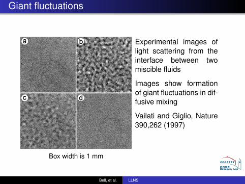
Box width is 1 mm

Experimental images oflight scattering from theinterface between twomiscible fluids

Images show formationof giant fluctuations in dif-fusive mixing

Vailati and Giglio, Nature390,262 (1997)

Bell, et al. LLNS

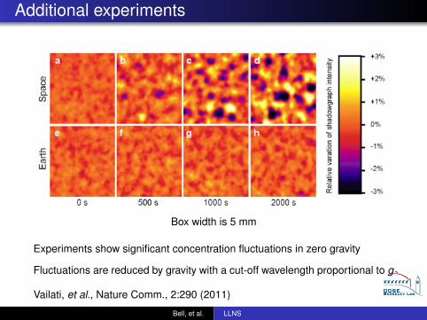
Additional experiments

Box width is 5 mm

Experiments show significant concentration fluctuations in zero gravity

Fluctuations are reduced by gravity with a cut-off wavelength proportional to g

Vailati, et al., Nature Comm., 2:290 (2011)

Bell, et al. LLNS

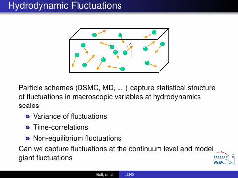
Hydrodynamic Fluctuations

Particle schemes (DSMC, MD, ... ) capture statistical structureof fluctuations in macroscopic variables at hydrodynamicsscales:

Variance of fluctuationsTime-correlationsNon-equilibrium fluctuations

Can we capture fluctuations at the continuum level and modelgiant fluctuations

Bell, et al. LLNS

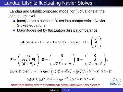
Landau-Lifshitz fluctuating Navier Stokes

Landau and Lifshitz proposed model for fluctuations at thecontinuum level

Incorporate stochastic fluxes into compressible NavierStokes equationsMagnitudes set by fluctuation dissipation balance

∂U/∂t +∇ · F = ∇ · D +∇ · S where U =

ρJE

F =

ρvρvv + PI(E + P)v

D =

0τ

κ∇T + τ · v

S =

0S

Q+ v · S

,

〈Sij (r, t)Sk`(r′, t ′)〉 = 2kBηT(δK

ik δKj` + δK

i`δKjk − 2

3δKij δ

Kk`

)δ(r− r′)δ(t − t ′),

〈Qi (r, t)Qj (r′, t ′)〉 = 2kBκT 2δKij δ(r− r′)δ(t − t ′),

Note that there are mathematical difficulties with this systemBell, et al. LLNS

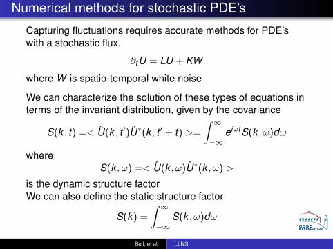
Numerical methods for stochastic PDE’s

Capturing fluctuations requires accurate methods for PDE’swith a stochastic flux.

∂tU = LU + KW

where W is spatio-temporal white noise

We can characterize the solution of these types of equations interms of the invariant distribution, given by the covariance

S(k , t) =< U(k , t ′)U∗(k , t ′ + t) >=

∫ ∞−∞

eiωtS(k , ω)dω

whereS(k , ω) =< U(k , ω)U∗(k , ω) >

is the dynamic structure factorWe can also define the static structure factor

S(k) =

∫ ∞−∞

S(k , ω)dω

Bell, et al. LLNS

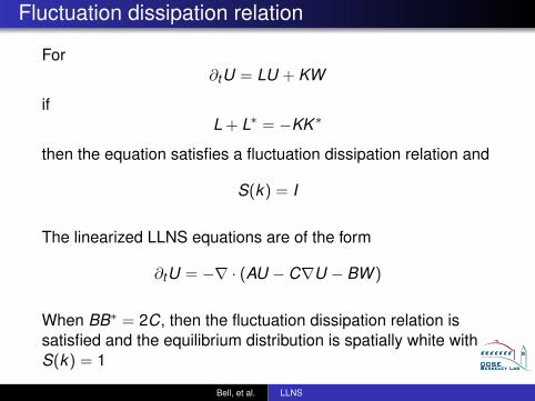
Fluctuation dissipation relation

For∂tU = LU + KW

ifL + L∗ = −KK ∗

then the equation satisfies a fluctuation dissipation relation and

S(k) = I

The linearized LLNS equations are of the form

∂tU = −∇ · (AU − C∇U − BW )

When BB∗ = 2C, then the fluctuation dissipation relation issatisfied and the equilibrium distribution is spatially white withS(k) = 1

Bell, et al. LLNS

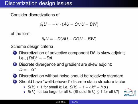
Discretization design issues

Consider discretizations of

∂tU = −∇ · (AU − C∇U − BW )

of the form∂tU = −D(AU − CGU − BW )

Scheme design criteria1 Discretization of advective component DA is skew adjoint;

i.e., (DA)∗ = −DA2 Discrete divergence and gradient are skew adjoint:

D = −G∗

3 Discretization without noise should be relatively standard4 Should have “well-behaved” discrete static structure factor

S(k) ≈ 1 for small k ; i.e. S(k) = 1 + αkp + h.o.tS(k) not too large for all k . (Should S(k) ≤ 1 for all k?)

Bell, et al. LLNS

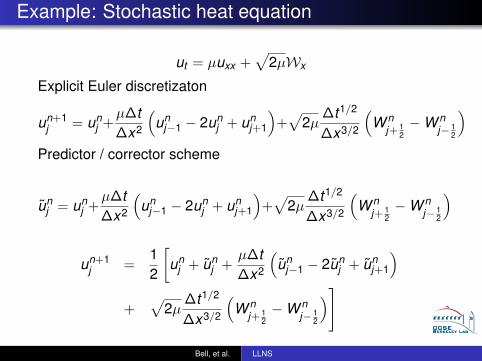
Example: Stochastic heat equation

ut = µuxx +√

2µWx

Explicit Euler discretizaton

un+1j = un

j +µ∆t∆x2

(un

j−1 − 2unj + un

j+1

)+√

2µ∆t1/2

∆x3/2

(W n

j+ 12−W n

j− 12

)Predictor / corrector scheme

unj = un

j +µ∆t∆x2

(un

j−1 − 2unj + un

j+1

)+√

2µ∆t1/2

∆x3/2

(W n

j+ 12−W n

j− 12

)

un+1j =

12

[un

j + unj +

µ∆t∆x2

(un

j−1 − 2unj + un

j+1

)+

√2µ

∆t1/2

∆x3/2

(W n

j+ 12−W n

j− 12

)]

Bell, et al. LLNS

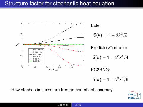
Structure factor for stochastic heat equation

0 0.2 0.4 0.6 0.8 1

k / kmax

0

0.5

1

1.5

2

Sk

b=0.125 E ulerb=0.25 E ulerb=0.125 PCb=0.25 PCb=0.5 PCb=0 (I deal)

Euler

S(k) = 1 + βk2/2

Predictor/Corrector

S(k) = 1− β2k4/4

PC2RNG:

S(k) = 1 + β3k6/8

How stochastic fluxes are treated can effect accuracy

Bell, et al. LLNS

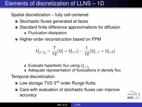
Elements of discretization of LLNS – 1D

Spatial discretization – fully cell-centeredStochastic fluxes generated at facesStandard finite difference approximations for diffusion

Fluctuation dissipation

Higher-order reconstruction based on PPM

UJ+1/2=

712

(Uj + Uj+1)− 112

(Uj−1 + Uj+2)

Evaluate hyperbolic flux using Uj+1/2Adequate representation of fluctuations in density flux

Temporal discretizationLow storage TVD 3rd order Runge KuttaCare with evaluation of stochastic fluxes can improveaccuracy

Bell, et al. LLNS

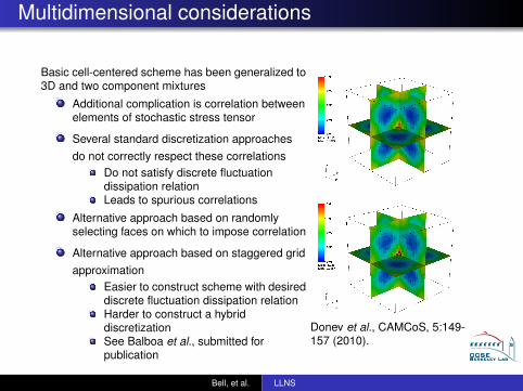
Multidimensional considerations

Basic cell-centered scheme has been generalized to3D and two component mixtures

Additional complication is correlation betweenelements of stochastic stress tensor

Several standard discretization approachesdo not correctly respect these correlations

Do not satisfy discrete fluctuationdissipation relationLeads to spurious correlations

Alternative approach based on randomlyselecting faces on which to impose correlation

Alternative approach based on staggered gridapproximation

Easier to construct scheme with desireddiscrete fluctuation dissipation relationHarder to construct a hybriddiscretizationSee Balboa et al., submitted forpublication

Donev et al., CAMCoS, 5:149-157 (2010).

Bell, et al. LLNS

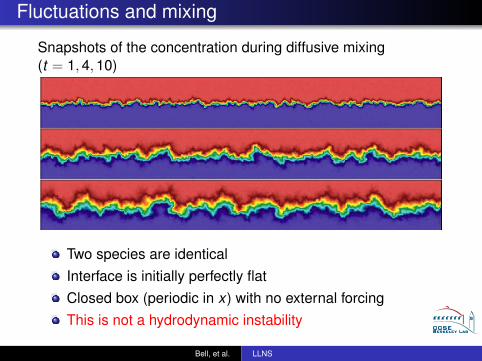
Fluctuations and mixing

Snapshots of the concentration during diffusive mixing(t = 1,4,10)

Two species are identicalInterface is initially perfectly flatClosed box (periodic in x) with no external forcingThis is not a hydrodynamic instability

Bell, et al. LLNS

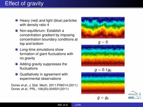
Effect of gravity

Heavy (red) and light (blue) particleswith density ratio 4

Non-equilibrium: Establish aconcentration gradient by imposingconcentration boundary conditions attop and bottom

Long-time simulations showformation of giant fluctuations withno gravity

Adding gravity suppresses thefluctuations

Qualitatively in agreement withexperimental observations

Donev et al., J. Stat. Mech. 2011:P06014 (2011)Donev et al., PRL, 106(20):204501(2011)

g = 0

g = 0.1g0

g = g0

Bell, et al. LLNS

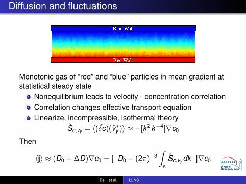
Diffusion and fluctuations

Monotonic gas of “red” and “blue” particles in mean gradient atstatistical steady state

Nonequilibrium leads to velocity - concentration correlationCorrelation changes effective transport equationLinearize, incompressible, isothermal theory

Sc,vy = 〈(δc)(v∗y )〉 ≈ −[k2⊥k−4]∇c0

Then

〈j〉 ≈ (D0 + ∆D)∇c0 = [ D0 − (2π)−3∫

kSc,vy dk ]∇c0

Bell, et al. LLNS

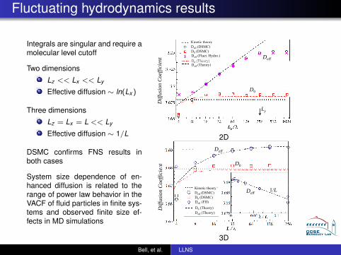
Fluctuating hydrodynamics results

Integrals are singular and require amolecular level cutoff

Two dimensions

Lz << Lx << Ly

Effective diffusion ∼ ln(Lx )

Three dimensions

Lz = Lx = L << Ly

Effective diffusion ∼ 1/L

DSMC confirms FNS results inboth cases

System size dependence of en-hanced diffusion is related to therange of power law behavior in theVACF of fluid particles in finite sys-tems and observed finite size ef-fects in MD simulations

Fluctuating Hydro. Solver Resultsg y

Kinetic theory

Deff

yDeff (DSMC)D0 (DSMC)Deff (Fluct. Hydro.)D (Theory)

Quasi-2D (Lz << Ly)

nt D0 (Theory)Deff (Theory)

Ly

Coe

ffici

en

D0 LxLz

ffusi

on C

Ly

Diff

Ly = 256 Lz = 2

2DFull 3D SystemsFull 3D Systems

Full 3D (L L )D ffD (Lx = Lz)

DeffDeff

D0ntLy

D

Coe

ffici

en

Lx

LzDeffKinetic theoryDeff (DSMC)D0 (DSMC)Deff (FH)

Deff

ffusi

on C

Ly = Lz = L1/L

eff ( )D0 (Theory)Deff (Theory)

ΔD goes as1/L0 – 1/L

Diff

3DBell, et al. LLNS

SummaryCorrelation of fluctuations that leads to enhanced diffusion can also lead tomacroscale observables in diffusive mixing (giant fluctuations)

Effect is relatively small in gasesSignficantly enhanced for liquids or additional physics such as reactionsFluctuations can play a key role in the design of microfluidic devices

Numerical methodology for fluctuating Navier Stokes equationsHiger-order centered discretization of advection (skew adjoint)Second-order centered approximation of diffusion (self adjoint)RK3 centered schemeResulting discretization satisfies discrete fluctuation dissipation resultDiscretization designed to have well-behaved discrete static structurefactorsFNS solver is able to capture enhancement of diffusion resulting fromfluctuations

Future directionsFluctuations in low Mach number flowsFluctuations in reacting systems

Bell, et al. LLNS

Hybrid approach

Develop a hybrid algorithm for fluid mechanics that couples aparticle description to a continuum description

Molecular model only where needed – DSMCCheaper continuum model in the bulk of the domain –LLNS

AMR provides a framework for such a couplingAMR for fluids except change to a particle description at thefinest level of the heirarchy

Use basic AMR design paradigm for development of ahybrid method

Bell, et al. LLNS

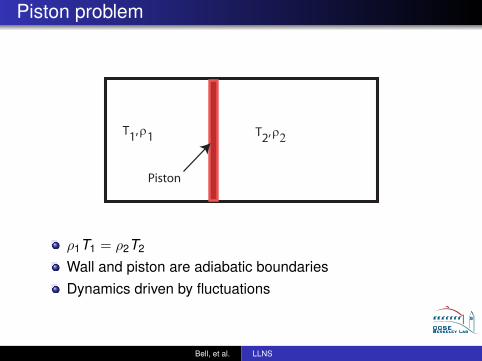
Piston problem

T1, ρ1 T2, ρ2

Piston

ρ1T1 = ρ2T2

Wall and piston are adiabatic boundariesDynamics driven by fluctuations

Bell, et al. LLNS

Piston dynamics

Hybrid simulation of PistonSmall DSMC region near the pistonEither deterministic or fluctuating continuum solver

Bell, et al. LLNS

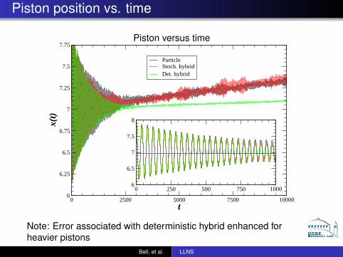
Piston position vs. time

Piston versus time

0 2500 5000 7500 10000t

6

6.25

6.5

6.75

7

7.25

7.5

7.75x(

t)ParticleStoch. hybridDet. hybrid

0 250 500 750 10006

6.5

7

7.5

8

Note: Error associated with deterministic hybrid enhanced forheavier pistons

Bell, et al. LLNS