lorentz violation, causality, and black holes

Thomas P. Sotiriou !

based on work with: Enrico Barausse, Jishnu Bhattacharyya, Mattia Colombo, Ted Jacobson, Ian Vega, Daniele Vernieri

Lorentz violation, causality, and black holes

LV and causal structure

Causal structure in special relativity

� � k

LV with linear dispersion relations

Different modes have different speeds and different “light” cones

But there are still “light” cones!

Thomas P. Sotiriou - Galiano, Aug 19th 2015

Einstein-aether theory

Sæ =1

16�Gæ

�d4x

⇥�g(�R�M�⇥µ⌅⇤�uµ⇤⇥u⌅)

M�⇥µ⌅ = c1g�⇥gµ⌅ + c2g

�µg⇥⌅ + c3g�⌅g⇥µ + c4u

�u⇥gµ⌅

The action of the theory is

where

and the aether is implicitly assumed to satisfy the constraint

uµuµ = 1

Most general theory with a unit timelike vector field which is second order in derivatives

T. Jacobson and D. Mattingly, Phys. Rev. D 64, 024028 (2001).


Einstein-aether theory

Extensively tested and still viable

It propagates a spin-2, a spin-1 and spin-0 mode.

Linear dispersion relations.

These modes travel at different speeds.

We expect multiple horizons!


LV and black hole structure

What happens to black holes?

They will have multiple horizons!


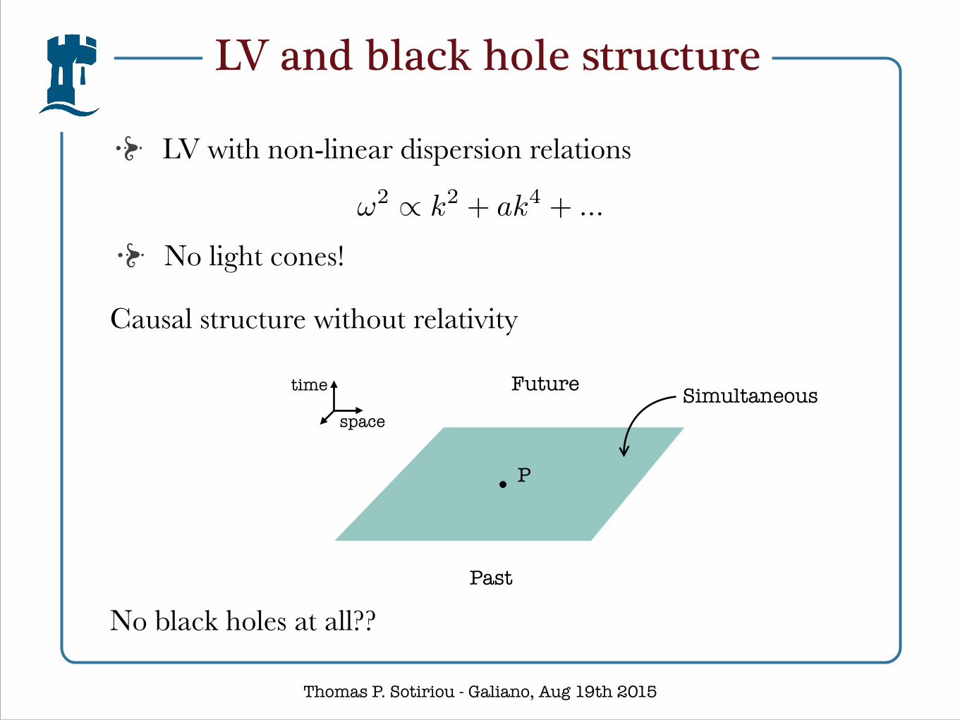
Causal structure without relativity

space

time

P

Past

Future Simultaneous

LV with non-linear dispersion relations

No black holes at all??

�2 � k2 + ak4 + ...

No light cones!

LV and black hole structure


Hypersurface orthogonality

Now assume u� =��T�

gµ⇤�µT�⇤T

and choose as the time coordinate

u� = ��T (gTT )�1/2 = N��T

Replacing in the action and defining one gets

with and the parameter correspondenceGH

Gæ= ⇤ =

1

1� c13⇥ =

1 + c21� c13

� =c14

1� c13

ai = �i lnN

Shoæ =

1

16⌅GH

⇤dTd3xN

⇥h�KijK

ij�⇥K2+⇤(3)R+ �aiai⇥

T

T. Jacobson, Phys. Rev. D 81, 101502 (2010).


Horava-Lifshitz gravity

The action of the theory is

SHL =1

16�GH

�dTd3xN

�h( L2 +

1

M2�

L4 +1

M4�

L6)

where

L2 = KijKij � ⇥K2 + ⇤(3)R+ �aia

i

contains all 6th order terms constructed in the same wayL6 :

L4 : contains all 4th order terms constructed with the induced metric andhij ai

P. Hořava, Phys. Rev. D 79, 084008 (2009) D. Blas, 0. Pujolas and S. Sibiryakov, Phys. Rev. Let. 104, 181302 (2010)


Horava-Lifshitz gravity

Higher order terms contain higher order spatial derivatives: higher order dispersion relations!

They modify the propagator and render the theory power-counting renormalizable

All terms consistent with the symmetries will be generated by radiative corrections

This version of the theory is viable so far

“Low energy limit” is h.o. Einstein-aether theory!

We expect no causal boundaries!


Spacetime diagram Si

ngul

arit

y

Universal Horizon Metric Horizon r

t

Constant preferred time

E. Barausse, T. Jacobson and T.P.S., Phys. Rev. D 83, 124043 (2011)


Penrose diagram

Taken from D. Blas and S. Sibiryakov, Phys. Rev. D 84, 124043 (2011) !!!!!

φ

i+

i0�� = ��

Figure 2: The leaves of constant khronon field (thin solid lines) superimposed on the upper

half of the Penrose diagram of the Schwarzschild black hole. The thick solid line shows the

universal horizon.

signals, no matter how fast, can propagate only forward in this global time. In this way

the configuration of the khronon determines the causal structure of space-time in Horava

gravity. From Fig. 2 it is clear that within this causal structure the inner region � > �⇥ lies

in the future with respect to the outer part of the space-time. Thus no signal can escape

from inside the surface � = �⇥ to infinity (null asymptotic region between i+ and i0) meaning

that this surface is indeed a universal horizon, cf. [26].

It should be pointed out that within the spherically symmetric approximation that we

have adopted so far the universal horizon is regular, despite the apparent singularity (45)

of the khronon. Indeed, we have seen above that the field uµ, which is the proper invariant

observable of the theory, is smooth at � = �⇥. This implies that the singularity (45) can

be removed by the symmetry transformation of the form (2). It is easy to see that the

transformation

⇥ ⇤⇥ ⇥ = exp�(�2⇥U

�⇥

⇤�⇥ � 1) ⇥

⇥

does the job: the redefined khronon field is analytic at �⇥. However, in the next section

we will argue that the universal horizon exhibits non-linear instability against aspherical

perturbations of the khronon field, which turn it into a physical singularity.

17

Universal HorizonT


Rotating black holes

T.P.S., I. Vega and D. Vernieri, Phys. Rev. D 90, 044046 (2014) !!!!


Slowly rotating BHs in Einstein-aether theory do not have a preferred foliation.

Slowly rotating BHs in Horava gravity have universal horizons.

3d rotating black holes can have universal horizons even with flat asymptotics.

Universal horizons can lie “outside” de Sitter horizons.

T.P.S. and E. Barausse, Phys. Rev. Lett. 109, 181101 (2012) T.P.S. and E. Barausse, Phys. Rev. D 87, 087504 (2013)

T.P.S. and E. Barausse, Class. Quant. Grav 30, 244010 (2013) !!!

What’s next?

A new “toolkit” is needed

How do we define this horizon in full generality?

Can we have a local definition when we have less symmetry?

Is the universal horizon relevant to astrophysics?

M. Colombo, J. Bhattacharyya, and T.P.S., arXiv:1508.???? [gr-qc] !!!


Causally preferred foliation

Consider a manifold with a preferred foliationDefinition: Ordered foliation

Every event in lies on a unique leaf

Every pair of events has a unique causal relation

No preferred labeling implies invariance under T ! T (T )

Definition: Causal and acausal curves

causal, future directed if causal, past directed if acausal if

Continuous, piecewise differentiable curve with tangent

uµtµ > 0

uµtµ < 0

uµtµ = 0

(M ,⌃, g)

M

tµ


Future and Past

Definition: Future and Past

The future of an event is the set of all events that can be reached from by a future directed causal curve.

J+(p) pp

Similarly for the Past.10 J. BHATTACHARYYA, M. COLOMBO, AND T. P. SOTIRIOU

J+(p)

p

J+(S)

S

(a)

p

J+(p) = J+(⌃p)

⌃p Sp

(b)

Figure 1. Di↵erence between the notions of and causal future inlocally Lorentz invariant theories (A) and theories with a preferredfoliation (B).

is devoted towards uncovering those unique features of causality in a foliated mani-fold which drastically contrast those of general relativity. As we already saw above,curves that are arbitrarily spacelike with respect to gab may still represent causalcurves here. One of the rather remarkable consequences of the existence of suchcurves and our definition of future (past) is that the future (past) of every event isidentical with the future (past) of the leaf on which the event resides or that of anysimset of the leaf, i.e.

J+(p) = J+(⌃p) = J+(Sq) ,

J�(p) = J�(⌃p) = J�(Sq) , 8p 2 M , 8q 2 ⌃p .(13)

We will conclude this section with some comments and observations on theopen/closed-ness of the sets J±(⌃p) and related properties of their respective clo-sures. Consider the set J+(⌃p) to begin with. Since the whole spacetime is openby assumption, J+(⌃p) cannot contain any ‘boundary events’, i.e. every eventq 2 J+(⌃p) should admit at least one open neighbourhood Oq ✓ J+(⌃p); moreformally, one may invoke the results of Theorem 8.1.2 of Ref. [33] (see also Propo-sition 2.8 of Ref. [31] or Lemma 14.2 of Ref. [34]) in order to construct a proof ofthis. Therefore J+(⌃p) is an open set.

The fact that J+(⌃p) is open can also be deduced in a more intuitive fashion as

follows: the speed-c metric g(c)ab of eq. (8) allows us to formally associate an open

set I+(c)(p) – the general relativistic chronological future of p constructed with g(c)ab –

at every event p 2 M . The collection {I+(c)(p) | c > 0} then forms an open cover of

J+(p) such that J+(p) = [c>0I+(c)(p). Therefore J

+(p), and hence J+(⌃p) by virtue

of eq. (13), are open. We should emphasize that the open sets I+(c)(p) have been

used as pure mathematical objects in the above argument; in particular, they haveno physical significance in regards to the causality of the backgrounds, either hereor in what follows. However, the proof does rest on the intuitive picture that in alocally Lorentz invariance violating geometry, causal curves are no longer containedin any fixed propagation cones, and that the leaves of the foliation are the resultof ‘opening up/flattening out’ of the local propagation cones to their maximum intheir attempt to contain these causal curves within them.


Asymptotics

What’s the analogue of asymptotic flatness?

Conformally extended manifold:

projector:

point as spatial infinity of :

pµ⌫ = gµ⌫ � uµu⌫

⌃p ⌃p = ⌃p [ ipip

One also needs conditions for the foliation!

Key concept: ‘trivially foliated asymptotically flat end’

I =[

p2hhMii

ip

hhM ii : open region in which every leaf has trivially foliated asymptotically flat end

M , pµ⌫ = ⌦2pµ⌫


Universal horizons

Future and past event horizons:

H+ ⌘ @J�(I ) H� ⌘ @J+(I )

It follows that

hhM ii = J�(I ) \ J+(I )

H±

are leaves and boundaries of hhM ii

Key point:

Black hole:

White hole:

B(I ) ⌘ M \ J�(I )

W(I ) ⌘ M \ J+(I )

H±(I ) \ I = 0


Local characterisation

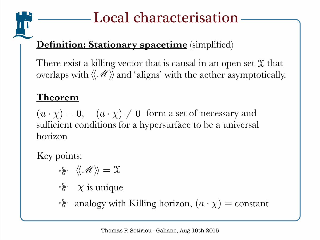
Definition: Stationary spacetime (simplified)

There exist a killing vector that is causal in an open set that overlaps with and ‘aligns’ with the aether asymptotically.hhM ii

Theorem form a set of necessary and sufficient conditions for a hypersurface to be a universal horizon

(u · �) = 0, (a · �) 6= 0

X

hhM ii = X

Key points: is unique analogy with Killing horizon, constant

�

(a · �) =


Astrophysical relevance

Assume also axisymmetry

(u · ') = (a · ') = 0

Suppose there is a universal horizonDoes there need to be a Killing horizon? Does is cloak the universal horizon?

V µ ⌘ �µ +W'µ W ⌘ �(� · ')/(' · ') (V · ') = 0

�[µ'⌫r'�] = 0 '[µ�⌫r��] = 0Iff

then by Carter’s rigidity theorem

(V · V ) = 0 W =is a null hypersurface where constant


Perspectives

Black holes are of great interest in Lorentz-violating theories. New notion: “universal horizon”

Non-trivial causal structure

Is this horizon stable?

Does it form from collapse?

M. Saravani, N. Afshordi and R. B. Mann, Phys. Rev. D 89, 084029 (2014) !!!!

D. Blas and S. Sibiryakov, Phys. Rev. D 84, 124043 (2011) !!!!!


lorentz violation, causality, and black holes

Documents