loop 289 corridor study - phase ii - texas tech · loop 289 corridor study - phase ii . loop 289...

TechMRT

Texas Tech University

8/31/2012

Loop 289 Corridor Study - Phase II

Loop 289 Corridor Study – Phase II

by

Hao Xu

Hongchao Liu

Wesley Kumfer

Dali Wei

Hiron Fernando

Henok Tezera

A research project sponsored by the

City of Lubbock

Metropolitan Planning Organization

ii

TABLE OF CONTENTS

LIST OF TABLES ......................................................................................................................... IV

LIST OF FIGURES ......................................................................................................................... V

1. INTRODUCTION ................................................................................................................... 1

1.1 BACKGROUND AND LITERATURE REVIEW ......................................................................... 2

1.2 PHASE I STUDY ................................................................................................................. 6

1.3 OBJECTIVE OF PHASE 2 PROJECT ....................................................................................... 9

1.4 DESCRIPTION OF ALTERNATIVES AND MODEL MODIFICATIONS ........................................ 9

1.5 METHODOLOGICAL APPROACH ....................................................................................... 14

1.6 SUMMARY OF RESULTS AND RECOMMENDATIONS ......................................................... 16

1.7 ORGANIZATION OF THE REPORT ...................................................................................... 22

2. TRAFFIC DATA AND DATA MINING ............................................................................. 23

2.1. DATA COLLECTION ......................................................................................................... 23

2.2. DATA ANALYSIS ............................................................................................................. 32

3. ANALYSIS OF RAMP TRAFFIC REDISTRIBUTION ...................................................... 34

3.1 RAMP DESIGN FOR DIAMOND TO X ................................................................................. 34

3.2 EASTBOUND ON- AND OFF- RAMPS ................................................................................. 36

3.3 WESTBOUND ON- AND OFF- RAMPS ................................................................................ 42

3.4 INTERCHANGE TRAFFIC VOLUME CHANGES ................................................................... 47

3.5 TRAFFIC RE-ROUTING RESULTS ALONG FRONTAGE ROADS ........................................... 49

4. MICROSCOPIC SIMULATION WITH VISSIM AND SYNCHRO ................................... 51

4.1 NETWORK CODING .......................................................................................................... 51

4.2 MODEL CALIBRATION AND VALIDATION ........................................................................ 56

5. LEVEL OF SERVICE ANALYSIS OF MAIN LANES AND FRONTAGE ROADS ......... 60

5.1 CURRENT CONDITION ...................................................................................................... 61

5.2 SECTION BY SECTION EVALUATION ON THE FRONTAGE ROADS OF THE IMPROVEMENT

ALTERNATIVES ............................................................................................................... 64

5.3 SUMMARY FOR THE CURRENT CONDITION ...................................................................... 74

5.4 LOS ANALYSIS FOR THE PROJECTED TRAFFIC ................................................................ 79

6. LEVEL OF SERVICE ANALYSIS OF INTERSECTIONS ................................................. 91

iii

6.1 DATA ANALYSIS ............................................................................................................. 91

6.2 SIGNAL TIMING DESIGN .................................................................................................. 94

6.3 ANALYSIS RESULTS......................................................................................................... 95

7. WEAVING AND RAMP ANALYSIS................................................................................ 100

7.1 RATIONALE ................................................................................................................... 100

7.2 METHODOLOGY ............................................................................................................ 100

7.3 PROCEDURE ................................................................................................................. 1001

7.4 STUDY RESULTS ............................................................................................................ 111

7.5 CONCLUSION ................................................................................................................. 115

8. CONCLUSIONS ................................................................................................................. 116

9. REFERENCES .................................................................................................................... 118

iv

LIST OF TABLES

Table 1-1: Section by Section Level of Service of Main lane Traffic under Current Condition ................ 17

Table 1-2: Section by Section Level of Service of Frontage Road under Current Condition ..................... 17

Table 1-3: Section by Section Level of Service Main lane Traffic as a Result of Alternative 1 ................ 18

Table 1-4: Section by Section Level of Service of Frontage Roads as a Result of Alternative 1 ............... 18

Table 1-5: Section by Section Level of Service of Main lane Traffic as a Result of Alternative 2 ............ 19


Table 1-7: Section by Section Level of Service of Main lane Traffic as a Result of Alternative 3 ............ 20


Table 2-1: Recounted Turning Movements at Quaker Avenue and Indiana Avenue Interchanges ............ 30

Table 2-2: Observed Traffic Volumes between Freeway Main Lanes and Areas along Frontage Roads

between Slide Road and Quaker Avenue ............................................................................................ 31

Table 3-1: Traffic Rerouting along Frontage Roads of South Loop 289 (Current Traffic Demand) .......... 49

Table 3-2: Traffic Rerouting along Frontage Roads of South Loop 289 (Forecasted Future Traffic

Demand) .............................................................................................................................................. 50

Table 4-1: Validation Calculation for AM Simulation and Main lane Volume .......................................... 58

Table 4-2: Validation Calculation for PM Simulation and Main lane Volume .......................................... 58

Table 5-1: LOS of Traffic on Frontage Roads and Main Lanes of Basic Network .................................... 75

Table 5-2: Comparison of LOS between Basic Network and Alternative 1 ............................................... 76



Table 5-5: Comparison of LOS in the Basic Network between Current and Future Traffic Conditions .... 82

Table 5-6: Comparison of LOS between the Basic Network and Alternative 1 ......................................... 84



Table 6-1: Current AM Traffic Volumes at Interchanges with Different Ramp Configurations ................ 92

Table 6-2: Current PM Traffic Volumes at Interchanges with Different Ramp Configurations ................ 92

Table 6-3: Forecasted AM Traffic Volumes at Interchanges with Different Ramp Configurations .......... 93

Table 6-4: Forecasted PM Traffic Volumes at Interchanges with Different Ramp Configurations ........... 93

Table 6-5: AM Signal Timing Plan............................................................................................................. 97

Table 6-6: PM Signal Timing Plan ............................................................................................................. 97

Table 6-7: AM LOS with Current Traffic Volumes at Interchanges with Different Ramp Configurations98

Table 6-8: PM LOS with Current Traffic Volumes at Interchanges with Different Ramp Configurations 98

Table 6-9: AM LOS with Forecasted Traffic Volumes at Interchanges with Different Ramp

Configurations ..................................................................................................................................... 99

Table 6-10: PM LOS with Forecasted Traffic Volumes at Interchanges with Different Ramp

Configurations ..................................................................................................................................... 99

Table 7-1: Existing Geometric Conditions - 2011 .................................................................................... 103

Table 7-2: Alternative 1 - Weaving Analysis on Existing Condition - 2011 ............................................ 104

Table 7-3: Alternative 2 - Ramp Junction Analysis on X Pattern - 2011 ................................................. 105

Table 7-4: Alternative 3 - Weaving Analysis on X Pattern - 2011 ........................................................... 106

Table 7-5: Existing Geometric Conditions - 2016 .................................................................................... 107

Table 7-6: Alternative 1 - Weaving Analysis on Existing Condition - 2016 ............................................ 108

v

Table 7-7: Alternative 2 - Ramp Junction Analysis on X Pattern - 2016 ................................................. 109

Table 7-8: Alternative 3 - Weaving Analysis on X Pattern – 2016 .......................................................... 110

Table 7-9: Analysis Summary – 2011/AM Peak ...................................................................................... 111

Table 7-10: Analysis Summary – 2011/PM Peak ..................................................................................... 112

Table 7-11: Analysis Summary – 2016/AM Peak .................................................................................... 113

Table 7-12: Analysis Summary – 2016/PM Peak ..................................................................................... 114

Table 7-13: LOS Criteria for Ramp Junctions .......................................................................................... 114

LIST OF FIGURES Figure 1-1: Map of the Study Area ............................................................................................................... 1

Figure 1-2: Diamond Pattern interchange at Indiana Avenue ..................................................................... 11

Figure 1-3: X pattern interchange at Slide Road Overpass ......................................................................... 11

Figure 1-4: Alternative #1: Auxiliary Lane Addition ................................................................................. 12

Figure 1-5: Alternative #2: Diamond to X Type Interchange Reconfiguration .......................................... 13

Figure 1-6: Alternative #3: Diamond to X Type Interchange and Auxiliary Lane Addition ...................... 14

Figure 2-1: Data Collection Points at Slide Road Intersection ................................................................... 23

Figure 2-2: Data Collection Points at Quaker Avenue Intersection ............................................................ 24

Figure 2-3: Data Collection Points at Indiana Avenue Intersection ........................................................... 24

Figure 2-4: Data Collection Points at University Avenue Intersection ....................................................... 25

Figure 2-5: Data Collection Points West of the Interstate 27 Intersection.................................................. 25

Figure 2-6: Main lane Data Collection Point at Spur 327 ........................................................................... 26

Figure 2-7: Main lane Data Collection Point at Memphis Avenue ............................................................. 27

Figure 2-8: Main lane Data Collection Point at Avenue P .......................................................................... 27

Figure 2-9: Daily Traffic Volumes at the Spur 327 Detector ..................................................................... 28

Figure 2-10: Daily Traffic Volumes at the Memphis Avenue Detector ..................................................... 28

Figure 2-11: Daily Traffic Volumes at the Avenue P Detector .................................................................. 29

Figure 2-12: Areas along Frontage Roads Generating (and Attracting) Traffic to (or from) Freeway Main

Lanes ................................................................................................................................................... 31

Figure 2-13: Main lane Traffic Volume Calculated at Each Collection Point ............................................ 32

Figure 3-1: Proposed X Type Ramp Design at the Interchange of Quaker Avenue and South Loop 289.. 35

Figure 3-2: Proposed X Type Ramp Design at the Interchange of Indiana Avenue and South Loop 289 . 35

Figure 3-3: Proposed X Type Ramp Design at the Interchange of University Avenue and South Loop 289

............................................................................................................................................................ 36

Figure 3-4: Proposed X Type Ramp Design on the East of the Interchange of University Avenue and

South Loop 289 ................................................................................................................................... 36

Figure 3-5: Traffic Re-Distribution of the Eastbound Off-Ramp Between Slide Road and Quaker Avenue

............................................................................................................................................................ 37

Figure 3-6: Traffic Re-Distribution of the Eastbound Off-Ramp between Quaker Avenue and Indiana

Avenue ................................................................................................................................................ 38

Figure 3-7: Traffic Re-Distribution of the Eastbound On-Ramp between Quaker Avenue and Indiana

Avenue ................................................................................................................................................ 39

vi

Figure 3-8: Traffic Re-Distribution of the Eastbound Off-Ramp between Indiana Avenue and University

Avenue ................................................................................................................................................ 40

Figure 3-9: Traffic Re-Distribution of the Eastbound On-Ramp between Indiana Avenue and University

Avenue ................................................................................................................................................ 41

Figure 3-10: Traffic Re-Distribution of the Eastbound Off-Ramp on the East of University Avenue ....... 41

Figure 3-11: Traffic Re-Distribution of the Eastbound On-Ramp on the East of University Avenue ........ 42

Figure 3-12: Traffic Re-Distribution of the Westbound Off-Ramp on the East of University Avenue ...... 43

Figure 3-13: Traffic Re-Distribution of the Westbound On-Ramp on the East of University Avenue ...... 43

Figure 3-14: Traffic Re-Distribution of the Westbound Off-Ramp between University Avenue and

Indiana Avenue ................................................................................................................................... 44

Figure 3-15: Traffic Re-Distribution of the Westbound On-Ramp between University Avenue and Indiana

Avenue ................................................................................................................................................ 45

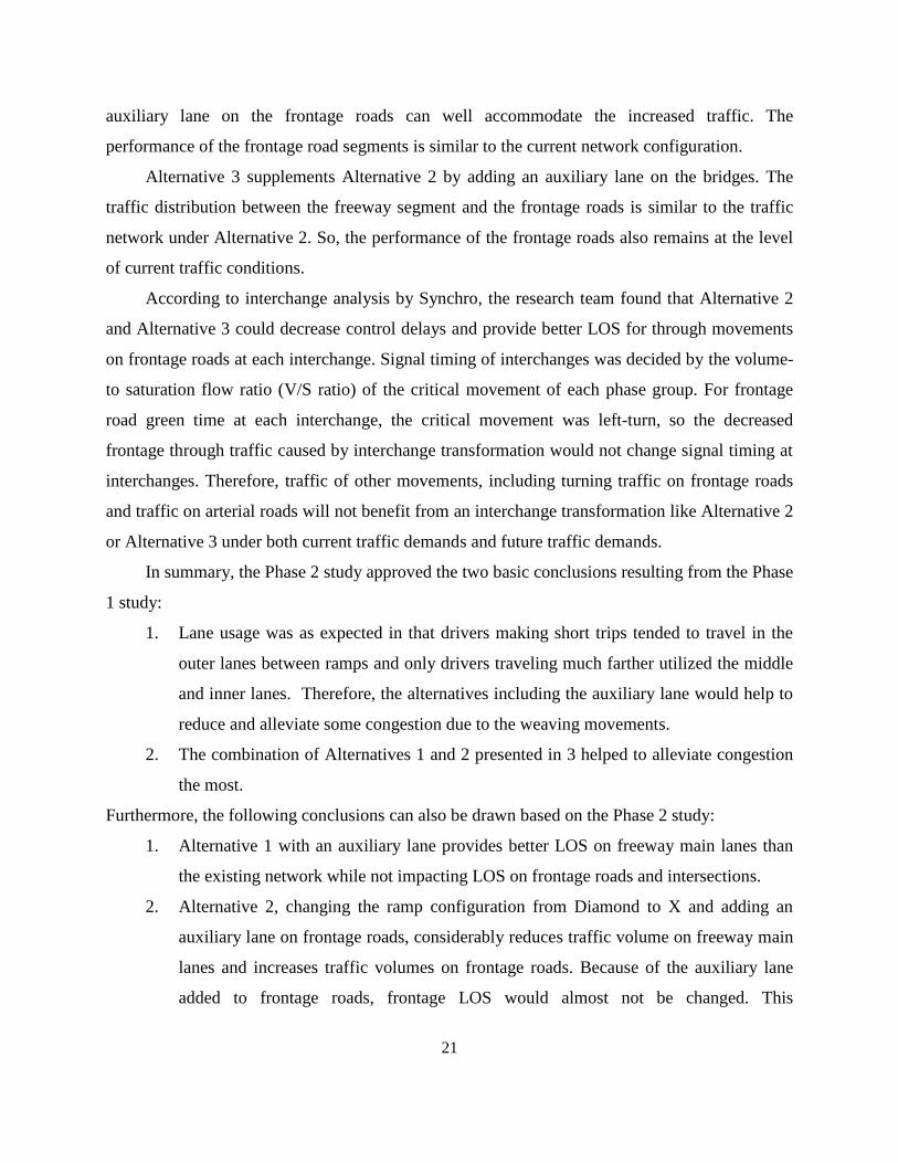
Figure 3-16: Traffic Re-Distribution of the Westbound Off-Ramp between Indiana Avenue and Quaker

Avenue ................................................................................................................................................ 46

Figure 3-17: Traffic Re-Distribution of the Westbound On-Ramp between Indiana Avenue and Quaker

Avenue ................................................................................................................................................ 47

Figure 3-18: Traffic Re-Distribution of the Westbound On-Ramp between Quaker Avenue and Slide

Road .................................................................................................................................................... 47

Figure 3-19: Business and Residential Areas Impacting Traffic Volumes of Through Movements .......... 48

Figure 4-1: Google Earth Image of the Project Area .................................................................................. 52

Figure 4-2: Coding of Traffic Control Systems at University Avenue ....................................................... 53

Figure 4-3: Snapshot of Simulation at University Avenue ......................................................................... 53

Figure 4-4: Screen Shot of the Synchro Model ........................................................................................... 54

Figure 4-6: Snapshot of Simulation at University Avenue ......................................................................... 56

Figure 4-7: AM Comparison of Actual to Simulation Volumes ................................................................. 59

Figure 4-8: PM Comparison of Actual to Simulation Volumes ................................................................. 59

Figure 5-1: Four Frontage Road Sections on the Network where the LOS Analysis is Conducted ........... 60

Figure 5-2: Five Main lane Sections on the Network where the LOS Analysis is Conducted ................... 61

Figure 5-3: V/C Ratio of Frontage Roads on the Basic Network (Westbound) ......................................... 62

Figure 5-4: Traffic Flow of Frontage Roads on the Basic Network (Westbound) ..................................... 62

Figure 5-5: Traffic Volumes on Main lane Segments on the Basic Network (Westbound) ....................... 63

Figure 5-6: Traffic Densities of Main lane Segments on the Basic Network (Westbound) ....................... 64

Figure 5-7: Traffic Volume on the Section FS1 for Differnet Alternatives ................................................ 65

Figure 5-8: V/C Ratio on the Section FS1 for Different Alternatives ....................................................... 66

Figure 5-9: Traffic Density on the Freeway Section MS1 for Different Alternatives ................................ 67

Figure 5-10: Traffic Density on the Freeway Section MS2 for Different Alternatives .............................. 67

Figure 5-11: Traffic Volumes on the Frontage Road Section FS2 for Different Alternatives .................... 68

Figure 5-12: V/C Ratio on the Section FS2 for Different Alternatives ..................................................... 69

Figure 5-13: Traffic Densities on the Freeway Section MS3 for Different Alternatives ............................ 70


Figure 5-15: V/C Ratio on the Section FS3 for Different Alternatives ..................................................... 71



vii

Figure 5-18: V/C Ratio on the Frontage Road Section FS4 for Different Alternatives ............................. 73


Figure 5-20: Traffic Volume on Main Lane Distribution on the Basic Network under Forecasted Traffic

Conditions in 2016 (Westbound) ........................................................................................................ 79

Figure 5-21: Traffic Densities on the Main Lanes of the Basic Network under Forecasted Traffic


Figure 5-22: Traffic Volumes on Frontage Roads of the Basic Network under Forecasted Traffic


Figure 5-23: V/C Ratios on Frontage Roads of the Basic Network for Current and Forecasted Traffic

Volumes (Westbound) ........................................................................................................................ 81

Figure 5-24: Effect of Alternative 1 on Frontage Roads with Current and Projected Traffic Data

(Westbound) ........................................................................................................................................ 83

Figure 5-25: Effect of Alternative 1 on Main Lane with Current and Projected Traffic Data (Westbound)

............................................................................................................................................................ 83


(Westbound) ........................................................................................................................................ 85

Figure 5-27: Effect of Alternative 2 on Main lane with Current and Projected Traffic Data (Westbound) 86

Figure 5-28: Effect of Alternative 3 on Traffic Volume and Lane Distribution with Current and Projected

Traffic Data (Westbound) ................................................................................................................... 88

Figure 5-29: Effect of Alternative 3 on Traffic Volume and Lane Distribution with Current and Projected

Traffic Data (Westbound) ................................................................................................................... 89

Figure 6-1: TTI-4-Phase Signal Timing Phase Design ............................................................................... 94

1

1. INTRODUCTION

South Loop 289 stretching from the I-27 interchange to Spur 327 is one of the busiest

corridors in Lubbock. It traverses the key business center of the city and includes four major

interchanges connecting with local arterial streets. The majority of the trips made in both peak

times of the day are short trips, which are less than the full length of the area between Slide Road

and Interstate 27. The congestion is concentrated toward the center of this area and peaks at

almost 100,000 vehicles per day.

This large traffic volume creates increased peak-hour congestion, traffic weaving, and

safety concerns. A very pressing issue is traffic control during congestion as the interchanges

and bridges are spaced within one mile of each other. This problem occurs at the grade for the

bridge sections, as the sight distance might be too short in order for some drivers to anticipate the

congestion ahead. When this occurs, accidents are often possible and might occur if drivers do

not take proper precautions to prevent them. Other than safety, planners are concerned with the

further increase in volumes and congestion in the area as the urban development of Lubbock is

moving much faster toward the South than any other direction. This will cause an increase in

volume for the South Loop 289 area far above what occurs in the present and will remain a

concern and problem if steps are not taken to alleviate the congestion. Contributing to the

operational problems are design deficiencies, such as the geometry and the type of the

interchanges, length of weaving sections, ramp tapers, and unevenly distributed traffic volumes

on main lanes. In addition, the closely spaced urban arterials intersecting with the loop system

and intensive commercial development along the route contribute to the problem.

Figure 1-1: Map of the Study Area

2

1.1 Background and Literature Review

Traffic congestion has grown steadily in the United States. Several recent studies indicate

that if trends do not change, most urban transportation networks will face frequent traffic

congestion problems. It is also stated in some studies that views on the design of urban streets

have been changing in response to economic, social, and environmental trends.

Among the ramp modification/reversal related research publications reviewed by the

research group, the Federal Highway Administration (FHWA) report conducted by Scott et al.

(2006) and publicized through the National Technical Information Service (NTIS) by the title

“Ramp Reversal Projects: Guidelines for Successful Implementation” was a key research

document because:

1) The study evaluated 15 ramp reversal projects on Texas freeways

2) The study investigated the benefit of ramp modification projects in many scenarios

3) The study provided 21 guidelines based on the evaluation conducted in the research.

The research project conducted by Nelson et al. on the “Lane Assignment Traffic Control

Device on the Frontage Roads and Conventional Roads at Interchanges” was also an important

case study under safe and efficient frontage road and intersection operation. The other study

reviewed, in detail, was the research document published by Klaver et al., which was conducted

on the “U.SOUTH 83 Main Lane, Ramp, and Cross-Street Interchange Operational Analysis”

(1995). It addressed the impact of widening of the main lanes and converting all ramps along the

study area to a uniform X-Ramp configuration. Other ramp modification related case study

projects were also reviewed and discussed under their corresponding topic.

In general, it was found that all the reviewed studies support the benefits of ramp

modification projects and addressed the X-Ramp pattern advantages under several viewpoints.

This literature review contains the findings of different studies on ramp modification

projects and their impacts on the frontage roads and intersection. The first part illustrates the

common motivations behind ramp modification projects as discussed in the reviewed studies.

The second part focuses on the impact of X-Ramp configurations on frontage roads and

intersections. The last part contains the challenges faced during ramp modification projects on

past research projects.

3

Desires for Ramp Modification Projects

Urban growth in general created the demand for the freeway system. The cost of

constructing new facilities or of expanding the existing ones was determined uneconomical and

as a last-case scenario in many recent projects. With main lane expansion becoming an ever-

diminishing possibility, many TxDOT districts have modified various freeway elements to

maximize efficiency and safety. In addition, it is crucial that the various improvement strategies

should be prioritized according to their expected cost effectiveness. Ramp modification projects

can also be categorized under those strategies of maximizing efficiency and safety.

Scott et al. (2006) discussed that ramp reversal or ramp modification projects become an

important consideration, especially when the situation involves traffic spilling back from an exit

ramp onto freeway main lanes. Congestion relief and improving traffic operations on freeway

main lanes are also mentioned as benefits on many ramp modification projects. Moreover,

improving access and traffic flow to the parks and malls was indicated as the driving force for

ramp modification projects like the IH 20 ramp reversal project in the City of Arlington.

Safety considerations, particularly at the cross-street/frontage road intersections are also

identified as primary factors for TxDOT to implement X-Ramp corridor projects at SH-358 in

Corpus Christi. Frawley (2005) discussed that managing access points along any type of roads

provides better mobility. In addition, Frawley illustrated how managing access points in state

highways provide better traffic flow. Managing access points creates opportunities for through-

traffic to brake and to accelerate in order to accommodate vehicles entering and exiting the

highway. The desire to commercially develop areas along frontage roads is also mentioned as the

main motivation behind to US 190 ramp reversal project in the City of Killeen.

Impact of X-Ramp Configuration on Frontage Roads and Intersections

In most of the ramp modification project case studies, the area between the exit ramp and

the upstream cross-street intersection is considered as the improved part of the frontage road.

The X-Ramp pattern configuration solves the congestion issue between the exit ramp/frontage

road intersection and the downstream cross-street. The improved segment on the frontage road

due to ramp reversal projects also helps to provide for better traffic flow on the cross-street

intersecting the frontage road.

4

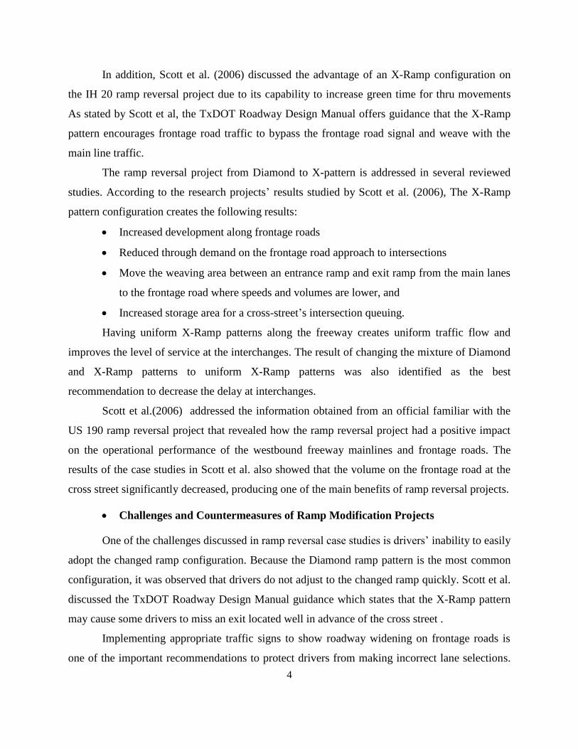
In addition, Scott et al. (2006) discussed the advantage of an X-Ramp configuration on

the IH 20 ramp reversal project due to its capability to increase green time for thru movements

As stated by Scott et al, the TxDOT Roadway Design Manual offers guidance that the X-Ramp

pattern encourages frontage road traffic to bypass the frontage road signal and weave with the

main line traffic.

The ramp reversal project from Diamond to X-pattern is addressed in several reviewed

studies. According to the research projects’ results studied by Scott et al. (2006), The X-Ramp

pattern configuration creates the following results:

Increased development along frontage roads

Reduced through demand on the frontage road approach to intersections

Move the weaving area between an entrance ramp and exit ramp from the main lanes

to the frontage road where speeds and volumes are lower, and

Increased storage area for a cross-street’s intersection queuing.

Having uniform X-Ramp patterns along the freeway creates uniform traffic flow and

improves the level of service at the interchanges. The result of changing the mixture of Diamond

and X-Ramp patterns to uniform X-Ramp patterns was also identified as the best

recommendation to decrease the delay at interchanges.

Scott et al.(2006) addressed the information obtained from an official familiar with the

US 190 ramp reversal project that revealed how the ramp reversal project had a positive impact

on the operational performance of the westbound freeway mainlines and frontage roads. The

results of the case studies in Scott et al. also showed that the volume on the frontage road at the

cross street significantly decreased, producing one of the main benefits of ramp reversal projects.

Challenges and Countermeasures of Ramp Modification Projects

One of the challenges discussed in ramp reversal case studies is drivers’ inability to easily

adopt the changed ramp configuration. Because the Diamond ramp pattern is the most common

configuration, it was observed that drivers do not adjust to the changed ramp quickly. Scott et al.

discussed the TxDOT Roadway Design Manual guidance which states that the X-Ramp pattern

may cause some drivers to miss an exit located well in advance of the cross street .

Implementing appropriate traffic signs to show roadway widening on frontage roads is

one of the important recommendations to protect drivers from making incorrect lane selections.

5

The SH114 ramp modification study in Grapevine also indicated that TxDOT maintenance staff

ultimately moved the exit ramp warning sign farther east on SH 114 to allow motorists more

time to react to the location of the new ramp. This may be a beneficial practice for similar

projects.

Selecting an appropriate microscopic simulation model for a ramp reversal project is also

a challenge and is one of the basic decision stages. Among the publicly or commercially

available microscopic simulation models, which are also discussed in the report by Scott et al.,

VISSIM and CORISM are mentioned as the most appropriate models for ramp modification

projects. Both models are considered practical candidates due to their route assignment features

so that vehicles can be routed from the freeway to the frontage road, or vice-versa, in such a

manner that unrealistic turning maneuvers are avoided.

The third challenge addressed in the reviewed case studies is the cost for the modification

project. Scott et al. (2006) indicated that construction of auxiliary lanes may require major

reconstruction at cross-streets. In addition, improving signal operations at the interchanges is also

indicated as a challenge on the project cost. Most of the case studies discussed by Scott et al.

indicated that signalized intersection operations must be adjusted in ramp reversal projects.

The road segment between the exit ramp and the subsequent entrance ramp was indicated

as the most critical and challenging area that should be closely analyzed during ramp reversal

projects. This area along the frontage road needs to be analyzed carefully because of the traffic

volume increase due to the exit ramp. The addition of an auxiliary lane on the frontage road is

considered the best option in most of the reviewed case studies and is an integral part of ramp

reversal projects.

Summary

The reviewed case studies indicated several motivations for implementing ramp reversal

projects. Traffic spilling back from an exit ramp onto freeway main lanes, congestion relief,

improved access and traffic flow to business centers, safety considerations (particularly at the

cross-street/frontage road intersections), and the need to commercially develop the area along the

frontage road are mentioned as the main reasons for ramp reversal projects.

The X-Ramp pattern interchange has been shown to be capable of solving the congestion

problem between the exit ramp/frontage road intersection and the downstream cross-street.

6

Additionally, X-Ramp patterns provide increased green time to thru movements. Increasing

development along a frontage road, reducing through demand on the frontage road approach to

the intersection, and increasing the storage area for the cross-street’s intersection queuing are

also included under the benefit of the X-Ramp pattern.

Moreover, the result of changing the mixture of Diamond and X-Ramp patterns to

uniform X-Ramp patterns was also identified as the best recommendation to decrease the delay

at the interchanges. The results of several ramp reversal case studies also showed that volumes

on the frontage road at the cross-street significantly decrease, leading to the other benefits of X-

ramp patterns. The area between the exit ramp and entrance ramp along the frontage road is

determined as the most vital area to be considered during a ramp reversal project. The addition of

an auxiliary lane on the frontage road was determined as the best option in most of the reviewed

case studies to overcome the increased volume from the entrance ramp.

Drivers’ inability to easily adopt the changed ramp, selecting an appropriate microscopic

simulation model, and project cost are mentioned as the main challenges for ramp modification

projects. Implementing appropriate traffic signs to show roadway widening on frontage roads,

using VISSIM and CORISM simulation models, and practicing cost effective construction

strategies are indicated as counter measures to address these issues.

In general, the reviewed case studies recommended that ramp modification projects are

worthwhile efforts. Moreover, the X-Ramp pattern was identified as the best scenario to provide

a positive impact on the operational performance of the freeway mainlines and frontage roads.

Implementing appropriate traffic signs to indicate the new ramp was also found as one of the

important recommendations to protect drivers from making an incorrect lane selection and to

avoid complaints.

1.2 Phase I Study

The first part of the study regarding congestion for Loop 289 was completed in 2007. The

study analyzed the level of service regarding the traffic volume in 2007 and modeled the

following alternatives to the interchange designs:

1. Keeping the existing ramp configurations, add an auxiliary lane to the outside main lane

between the entrance and exit ramps on the roadway segment between:

o Slide Avenue and Quaker Avenue

7

o Quaker Avenue and Indiana Avenue

o Indiana Avenue and University Avenue and

o University Avenue and I-27.

2. Convert the ramp configuration from diamond interchanges to X patterns along South

Loop 289, both east and west bound between:

o Quaker Avenue and Indiana Avenue

o Indiana Avenue and University Avenue and

o University Avenue and I-27

Depending on the simulation results, add a third lane on the frontage road connecting

exit and entrance ramps.

3. Alternative (2) with an additional auxiliary lane on the main lanes going over the

bridges.

These three alternative plans have advantages and disadvantages associated with cost, ease

of construction, and a reduction or relocation of congestions. The LOS analysis for the current

and forecasted traffic conditions were then conducted based on the simulation model developed

in VISSIM. The analysis work was performed in the following steps:

1. Analysis of current level of service (LOS)

The level of service of the South Loop 289 was determined for the current traffic volumes.

The LOS of the network was determined for five different sections, between the entrance and

exit ramps along the network. The LOS of each section was determined using HCS 2000, a

software package that follows the procedure defined in the Highway Capacity Manual 2000.

2. Analysis of LOS with proposed improvement alternatives

A set of simulation models representing the proposed improved alternative networks were

developed on the basis of the basic calibrated network. All these networks, including basic

networks, were modeled with the current traffic volumes, and the analysis of LOS was conducted

on the output volumes from the simulation networks. These volumes were converted to density

for the LOS analysis.

3. Analysis of LOS with the forecasted traffic volume

After the analysis of the alternatives with current traffic volumes, the current traffic

volumes were forecasted for five years at an annual growth rate of 3%. Then, all the simulation

8

networks were modeled with the forecasted volumes to analyze the traffic conditions that prevail

after five years on each of the networks.

Phase I resulted in several conclusions. Firstly, lane usage was as expected in that drivers

making short trips tended to travel in the outer lanes between ramps and only drivers traveling

much farther utilized the middle and inner lanes. This resulted in the hypothesis that the

alternatives including the auxiliary lane would help to reduce and alleviate some congestion due

to the weaving movements. The second and more important result is that the combination of

Alternatives 1 and 2 as presented in Alternative 3 helped to alleviate congestion the most.

The Phase I research revealed that the lane distribution on the main lanes is not evenly

distributed for the existing network and the network is congested at certain sections. Adding an

auxiliary lane to the main lanes, as in the case of Alternative 1, has provided better LOS than the

existing network, but could not create an even distribution of traffic on the main lanes. The

number of vehicles on the main lanes over the basic network and Alternative 1 is almost equal at

every section, as there is no change in ramp configuration between the two networks. Changing

the ramp configuration from Diamond to X, as in the case of Alternative 2, considerably reduced

the volume of traffic on the main lanes because an X- pattern interchange will transfer the

vehicles with shorter Origin-Destination trips (O-D) onto the frontage road, and this increased

the traffic volume on the frontage roads. However, this change in ramp configuration increased

the traffic volumes at the section between Slide and Quaker and at the Slide Road overpass. The

X-pattern interchange has provided an entrance ramp onto the main lanes instead of an exit ramp

at the section between Slide and Quaker. Alternative 3 provided better results compared to Basic

Network and Alternative 1, but not better than Alternative 2. Although the ramp configuration is

the same as Alternative 2 throughout the network, an auxiliary lane is provided on the main lanes

over the bridges in Alternative 3. This encouraged the high volume traffic on the frontage roads

to move onto the main lanes and hence the density on Alternative 3 is slightly higher than on

Alternative 2. So, it is concluded that Alternative 2 is the best alternative network among all the

three alternatives.

At the conclusion of this part of the study it was determined that to truly understand the

impact of the alternatives for the interchange design it would be necessary to make a more

detailed analysis of the frontage road segments. It was hypothesized that instead of using the

main lanes, some traffic might be using the frontage road segments instead. This would mean

9

that the reduction in congestion on the main lanes would then be moved to the frontage road

segments and would therefore undo the good caused by the alternatives. Phase 2 was determined

to be necessary to complete this analysis and further this conclusion by increasing its scope,

making the result more accurate.

1.3 Objective of Phase II Project

This Phase II study was conducted based on the Phase I study recommendation and

particularly focused on the impact of the ramp reversal strategy on frontage roads and

intersections. The study mainly addressed the evaluation of the level of service on the frontage

roads and intersections on the area of interest. It also identified best practices for frontage road

and intersection operation while implementing ramp modification projects.

In order to complete the analysis of the improvement options for South Loop congestion

issues, further literature review on X-pattern interchanges was performed. In this research, the

three alternatives presented in Phase I were analyzed by taking into consideration the frontage

road segments and the interchanges affected by the change in interchange design for both

morning and afternoon peaks. This was done to prove or disprove the hypothesis that drivers

were utilizing the frontage road segments for trips instead of the main lanes, reducing congestion

on the main lanes but increasing the congestion on the frontage road. This was taken further by

analyzing the impact to the South Loop and major arterial interchanges. It was determined

analytically that the traffic from freeway main lanes to areas along frontage roads (or traffic in

the opposite direction) will be re-routed. The traffic re-routing will cause a change in traffic

volumes on some ramps, frontage road segments, and frontage road through-traffic volumes at

interchanges. The changed traffic volumes were estimated according to traffic observations

between Slide Road and Quaker Avenue, where the ramps are already X-patterns. In regards to

these interchanges, optimized signal timing will also be analyzed and changed if needed. This

will take full advantage of any volume changes created by interchange design changes.

1.4 Description of Alternatives and Model Modifications

The original tasks of this project included the addition of an outside auxiliary lane to the

main lanes of South Loop 289 between each of the entrance and exit ramps from I-27 to Slide

Road, the conversion of the ramp configuration from X to Diamond pattern between Slide Road

and Quaker Avenue, as well as the conversion from Diamond to X pattern at the rest of the

10

interchanges. Based on the simulation results from the first phase of the work, three alternatives

were developed.

Alternative1 (A1): An auxiliary lane is added to the outside main lane between each entrance

and exit ramp on both eastbound and westbound directions at:

Slide Road and Quaker Avenue

Quaker Avenue and Indiana Avenue

Indiana Avenue and University Avenue

University Avenue and IH-27

Alternative 2 (A2): The ramp configuration of the basic network is changed from Diamond to X

pattern at:

Quaker Avenue

Indiana Avenue

University Avenue

Considering that providing an X pattern interchange will increase traffic volume on the

frontage road, an auxiliary lane is added on the frontage road between each exit and entrance

ramp.

Alternative 3 (A3): This alternative is developed by providing an auxiliary lane on the main

lanes to Alternative 2. The auxiliary lane is provided on the main lanes over the bridges for both

eastbound and westbound directions.

Diamond and X Pattern Interchanges

The project area consists of four major interchanges, consisting of one X pattern

interchange at the Slide Road overpass, two Diamond interchanges at University Avenue and

Indiana Avenue, and a combination of X and Diamond interchanges at Quaker Avenue.

Diamond Interchange: A Diamond interchange is a common type of interchange; it is generally

used when a freeway crosses a minor or major road. The freeway and the road are grade-

separated. For a Diamond interchange on either direction, an off-ramp diverges slightly from the

freeway and runs directly across the frontage road, becoming an on-ramp that returns to the

freeway in a similar fashion. A typical layout of a Diamond interchange is shown in Figure 1-2.

11

Figure 1-2: Diamond Pattern interchange at Indiana Avenue

X pattern Interchange: An X pattern interchange has a ramp configuration opposite to that of a

Diamond interchange. In the case of Diamond interchanges, an exit ramp is provided while

approaching the intersection and an entrance ramp following the intersection. In an X pattern

interchange, the entrance ramp is provided before the intersection, and the exit ramp is provided

after the interchange is crossed. A typical X interchange is shown in Figure 1-3:3.

Figure 1-3: X pattern interchange at Slide Road Overpass

12

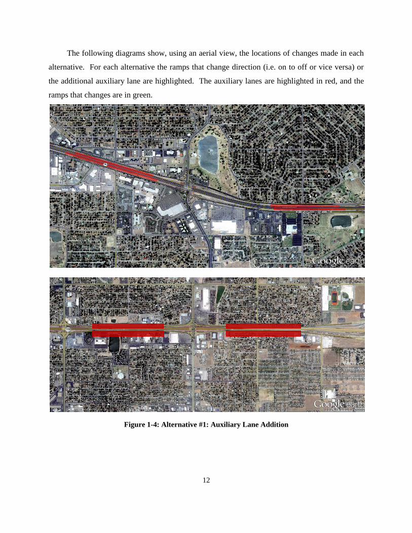
The following diagrams show, using an aerial view, the locations of changes made in each

alternative. For each alternative the ramps that change direction (i.e. on to off or vice versa) or

the additional auxiliary lane are highlighted. The auxiliary lanes are highlighted in red, and the

ramps that changes are in green.

Figure 1-4: Alternative #1: Auxiliary Lane Addition

13

Figure 1-5: Alternative #2: Diamond to X Type Interchange Reconfiguration

14

Figure 1-6: Alternative #3: Diamond to X Type Interchange and Auxiliary Lane Addition

1.5 Methodological Approach

To thoroughly evaluate the traffic performance on South Loop 289 including main lanes,

frontage roads, intersections and weaving sections, both analytical and simulation approaches

were applied.

The microscopic traffic simulation software VISSIM was used to model and analyze the

traffic conditions on the main lane and frontage roads, while the Synchro software was employed

to design traffic signal timing plans and evaluate the performance of the four major interchanges

along South Loop 289.

15

Network Coding

The basic geometry of the simulation networks were coded on aerial photographs of the

study area from Google Earth. Links and nodes are the two design parameters which are used to

develop a network in Synchro and VISSIM. Links are used to define the main lanes, frontage

roads, and ramps while the nodes are used to connect all the necessary links in the network.

Details such as speed limits and signal timing plans are coded in their respective ways for each

program to match the real world conditions or modified if needed for the different configurations.

In order to analyze the LOS for the different segments in question, several different

approaches were taken. Density was used as the measuring factor for the main lanes of Loop

289 and the volume to capacity (V/C) ratio was used for the frontage road segments.

Specifically in Synchro, the intersection LOS was calculated using the average control delay per

vehicle, which is widely used for evaluating intersection performance.

Modeling Control Devices

After coding the geometry of the network, control devices are defined in the simulation

model. They are the parameters which control the traffic flow in the simulation model. These

control devices include a variety of parameters including Signal Controllers, Stop signs, Priority

rules, Desired Speed Decisions, and Reduced Speed Decisions.

Calibration and Validation of the Simulation Model

After all the features in the network are modeled, the model parameters are calibrated to

make the simulation model replicate the real field conditions. The procedure by which the

parameters of the model are adjusted so that the simulated response agrees with the measured

field conditions is known as Model Calibration. Some of these parameters will have an effect on

the driving behavior, and some of them will have an effect on the speed and acceleration of the

vehicle. All these model parameters can be categorized into:

(1) Car following parameters

(2) Lane changing parameters

(3) Kinetic parameters

(4) Vehicle parameters

In order to gauge the accuracy of the simulation, validation and calibration needed to be

done. Phase II simulations were calibrated in a similar manner as in Phase I. This method

16

included taking cuts at sections, recording the traffic volumes in the simulation, and comparing

the results to the measured field volumes to see if they were statistically accurate.

Signal Timing Design

The research team designed signal timing phase orders based on the traditional TTI-4-

Phase Diamond interchange operation, which is used at most Diamond interchanges in the City

of Lubbock. The green time calculation method documented in Chapter 10 and Chapter 16 of the

Highway Capacity Manual (HCM) 2000 was applied for obtaining equalizing saturation degrees

of critical movements.

An Excel program was developed for calculating green time with the inputs of traffic

volumes and lane configurations of interchanges. Calculated green time for each phase was

adjusted based on minimum green time and pedestrian traveling time to get practical signal

timing plans.

Weaving Analysis

Analytical methods in HCM 2000 were used to evaluate the weaving performance along

South Loop 289 as a supplement to the LOS analysis by simulation.

1.6 Summary of Results and Recommendations

The LOS analysis for the frontage road as well as the intersections was carried out for the

basic network and the three alternative networks developed in the simulation arena. The basic

network represents the existing condition, while Alternative 1 (A1) was developed by adding an

auxiliary lane between each entrance and exit ramp on both Eastbound and Westbound

directions; Alternative 2 (A2) was developed by changing the ramp configuration from Diamond

to X- pattern and adding an additional lane on the frontage road between each exit and entrance

ramp; and Alternative 3 (A3) was developed based on Alternative 2, by adding an auxiliary lane

on the main lanes over the bridges.

Similarly to the Phase 1 study, the simulation analysis was conducted at five sections of the

main lanes including the Slide Road overpass, Slide Road and Quaker Avenue, Quaker Avenue

and Indiana Avenue, Indiana Avenue and University Avenue, and the section between University

Avenue and IH27. The section by section level of service was first determined based on both the

morning and afternoon peak traffic data on the basic network, which are shown in Table 1-1.

17

Table 1-1: Section by Section Level of Service of Main Lane Traffic under Current Condition

*Section 1

*Section 2

*Section 3

*Section 4

*Section 5

AM Westbound C B C C B

Eastbound C B C C C

PM Westbound C B D C C

Eastbound C B C C B

*Section 1 - Slide Road overpass

*Section 2 – Between Slide Road and Quaker Avenue

*Section 3 – Between Quaker Avenue and Indiana Avenue

*Section 4 – Between Indiana Avenue and University Avenue

*Section 5 – Between University Avenue and IH27

The analysis of LOS on the frontage roads was carried out at four sections, including the

frontage roads between Slide Road and Quaker Avenue (FS1), between Quaker and Indiana

Avenue (FS2), between Indiana and University Avenue (FS3), and the section between

University and IH27. The LOS for the morning and afternoon peak hours is summarized in Table

1-2: Section by Section Level of Service of Frontage Road under Current Condition.

Table 1-2: Section by Section Level of Service of Frontage Road under Current Condition

Section 1 Section 2 Section 3 Section 4

AM Westbound C C B C

Eastbound C C C C

PM Westbound C C B C

Eastbound C C C C





As analyzed in Phase 1, the three improvement strategies impact the level of service of the

network in different ways. Adding an auxiliary lane to the main lanes between entrance and exit

ramps provides better LOS than the existing network because of the increased roadway capacity.

However, it cannot result in a significant change in traffic distributions between frontage road

and freeway simply because the auxiliary lane essentially does impact travelers’ route choice

18

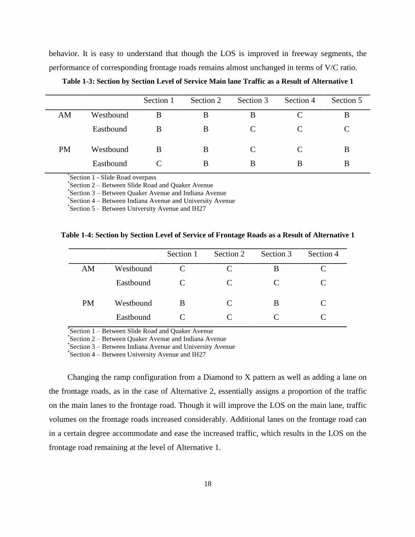
behavior. It is easy to understand that though the LOS is improved in freeway segments, the

performance of corresponding frontage roads remains almost unchanged in terms of V/C ratio.

Table 1-3: Section by Section Level of Service Main lane Traffic as a Result of Alternative 1

Section 1 Section 2 Section 3 Section 4 Section 5

AM Westbound B B B C B

Eastbound B B C C C

PM Westbound B B C C B

Eastbound C B B B B






Table 1-4: Section by Section Level of Service of Frontage Roads as a Result of Alternative 1



Eastbound C C C C

PM Westbound B C B C

Eastbound C C C C





Changing the ramp configuration from a Diamond to X pattern as well as adding a lane on

the frontage roads, as in the case of Alternative 2, essentially assigns a proportion of the traffic

on the main lanes to the frontage road. Though it will improve the LOS on the main lane, traffic

volumes on the frontage roads increased considerably. Additional lanes on the frontage road can

in a certain degree accommodate and ease the increased traffic, which results in the LOS on the

frontage road remaining at the level of Alternative 1.

19

Table 1-5: Section by Section Level of Service of Main lane Traffic as a Result of Alternative 2


AM Westbound C B C B B

Eastbound C B B C B

PM Westbound C B C C B

Eastbound C B C B B









Eastbound C C C C


Eastbound C C C C





In Alternative 3, the ramp configuration remains the same as in Alternative 2 throughout

the network, and an auxiliary lane is provided on the main lanes over the bridges rather than in

between the entrance and exit ramps. This alternative will improve the LOS on the overpass of

the interchanges but have little impact on freeway segments between interchanges including

Section 2, 3, 4 and 5.The pattern of traffic distribution between main lane and frontage roads

almost remains unchanged and the V/C ratios of the frontage roads are also similar when

compared with Alternative 2.

20

Table 1-7: Section by Section Level of Service of Main lane Traffic as a Result of Alternative 3


AM Westbound B B B B B

Eastbound B B B B B

PM Westbound B B C B B

Eastbound B B B B B









Eastbound C C C C


Eastbound C C C C





As analyzed in Phase 1, all three strategies will improve to varying degrees the level of

service on the main lanes of the corridor. However, they will bring different impacts on the

frontage roads.

Alternative 1 improves the level of service through added capacity on the main lanes of the

corridor. It will not affect the trip distribution along South Loop 289, which results in similar

traffic volumes and LOS on the frontage roads.

Alternative 2 alleviates the level of traffic density on the main lanes by converting the ramp

configuration from a Diamond to an X pattern. However, a certain proportion of trips,

particularly the short-distance trips, have been diverted to the frontage roads. Adding an

21

auxiliary lane on the frontage roads can well accommodate the increased traffic. The

performance of the frontage road segments is similar to the current network configuration.

Alternative 3 supplements Alternative 2 by adding an auxiliary lane on the bridges. The

traffic distribution between the freeway segment and the frontage roads is similar to the traffic

network under Alternative 2. So, the performance of the frontage roads also remains at the level

of current traffic conditions.

According to interchange analysis by Synchro, the research team found that Alternative 2

and Alternative 3 could decrease control delays and provide better LOS for through movements

on frontage roads at each interchange. Signal timing of interchanges was decided by the volume-

to saturation flow ratio (V/S ratio) of the critical movement of each phase group. For frontage

road green time at each interchange, the critical movement was left-turn, so the decreased

frontage through traffic caused by interchange transformation would not change signal timing at

interchanges. Therefore, traffic of other movements, including turning traffic on frontage roads

and traffic on arterial roads will not benefit from an interchange transformation like Alternative 2

or Alternative 3 under both current traffic demands and future traffic demands.

In summary, the Phase 2 study approved the two basic conclusions resulting from the Phase

1 study:

1. Lane usage was as expected in that drivers making short trips tended to travel in the

outer lanes between ramps and only drivers traveling much farther utilized the middle

and inner lanes. Therefore, the alternatives including the auxiliary lane would help to

reduce and alleviate some congestion due to the weaving movements.

2. The combination of Alternatives 1 and 2 presented in 3 helped to alleviate congestion

the most.

Furthermore, the following conclusions can also be drawn based on the Phase 2 study:

1. Alternative 1 with an auxiliary lane provides better LOS on freeway main lanes than

the existing network while not impacting LOS on frontage roads and intersections.

2. Alternative 2, changing the ramp configuration from Diamond to X and adding an

auxiliary lane on frontage roads, considerably reduces traffic volume on freeway main

lanes and increases traffic volumes on frontage roads. Because of the auxiliary lane

added to frontage roads, frontage LOS would almost not be changed. This

22

improvement option decreases frontage road through traffic at interchanges and

decreases control delay of this movement, but it has no effect on the other movements.

3. Alternative 3, with an auxiliary lane provided on freeway main lanes based on

Alternative 2, has provided the same LOS on frontage roads and at interchanges. The

auxiliary lane on the freeway benefited traffic from frontage roads to main lanes, while

encouraging through traffic on frontage roads to move onto the auxiliary lane of main

lanes. Alternative 3 provides better LOS on freeway main lanes and could further

decrease the frontage road through traffic at interchanges, which means lower control

delay and possibly better LOS for through traffic. However, the improvement option

would not benefit the other movements at interchanges.

4. With limited construction funding, the research team suggests Alternative 1 to

improve the traffic situation along South Loop 289.

5. With enough construction funding, the research team suggests Alternative 3, which

provides better LOS on main lanes, longer weaving distances for weaving traffic, and

better traffic safety at the joint points of on-ramps and main lanes.

1.7 Organization of the Report

This report contains eight sections. This section presents an overview of the project and

provides a detailed summary of the findings. Section Two discusses the data collection and data

analysis methods. Section Three presents an analytical discussion on the traffic redistribution

after converting the interchanges from Diamond to X-type. In section Four, the Vissim and

Synchro simulation tools used in the project are presented, as well as the description and

modeling of the network, and the calibration and validation of the simulation model. Section

Five presents the simulation results from Vissim and provides detailed LOS analysis of the

proposed alternative strategies. Section Six presents the results of the signal timing design, the

simulation results, and the LOS at the four major interchanges produced by Synchro. Section

Seven presents the weaving analysis of the freeway segment between on- and off-ramps for

current and future traffic volumes regarding the improved alternatives. Section Eight concludes

this study.

23

2. TRAFFIC DATA AND DATA MINING

2.1. Data Collection

In order to analyze the complex traffic flow in the South Loop 289 area, detailed data

needed to be collected. Traffic volumes needed to be collected at the following for all

interchanges:

Interchange Ramps

Arterial Intersection Approaches

Between Each Interchange Ramp and the Arterial Intersection Approach

Figures 2-1 through 2-5 show the locations where data was requested and received. For

each diagram, a location or interchange area is listed. Also in each figure, highlighted red areas

are frontage road data collection points, green areas are ramp locations, and blue areas are

intersection approach locations.

Figure 2-1: Data Collection Points at Slide Road Intersection

24

Figure 2-2: Data Collection Points at Quaker Avenue Intersection

Figure 2-3: Data Collection Points at Indiana Avenue Intersection

25

Figure 2-4: Data Collection Points at University Avenue Intersection

Figure 2-5: Data Collection Points West of the Interstate 27 Intersection

26

For each interchange related location, the volumes were provided in 15 minute intervals.

They were provided for a couple of days of the week and the AM or PM peak was listed. For the

Quaker and Indiana intersections, some of the existing data was missing or inaccurate, so this

was supplemented by collecting new data for the turning movements by hand in the field. This

new data was collected only at the peak times.

The collection of data for this analysis also provided easy access to detailed information of

the traffic volume on the main lanes. This was seen as a better alternative than relying strictly on

a growth factor for the current volume situation. The analysis used volumes collected at the

three TxDOT detector points on the South Loop. Figures 2-6 through 2-8 show the location of

the detectors and a description of the way in which the day is presented. Each lane is given a

number as shown in the figures.

Figure 2-6: Main lane Data Collection Point at Spur 327

EB W

B

27

Figure 2-7: Main lane Data Collection Point at Memphis Avenue

Figure 2-8: Main lane Data Collection Point at Avenue P

The TxDOT data from these detector locations were provided for three years in a volume

per day measurement. Some data provided was erroneous and was listed as such in the

information provided. Erroneous information was taken out of the data for the analysis.

The city’s traffic volumes are presented in an interesting way. The traffic volumes from the

City of Lubbock are plotted year versus year per lane in order to grasp a sense of increasing or

decreasing traffic volume as presented in Figures 2-9 through 2-11.

EB

W

B

EB

W

B

28

Figure 2-9: Daily Traffic Volumes at the Spur 327 Detector

Figure 2-10: Daily Traffic Volumes at the Memphis Avenue Detector

0

2000

4000

6000

8000

10000

12000

WB

Ou

t

WB

Mid

WB

In

EB In

EB M

id

EB O

ut

EB R

amp

Ave

rage

Dai

ly V

olu

me

Spur 327- Lane Traffic Volume

Avg 2008

Avg 2009

Avg 2010

Avg 2011

0

5000

10000

15000

20000

25000

EB O

ut

EB M

id

EB In

WB

In

WB

Mid

WB

Ou

t

Ave

rage

Dai

ly V

olu

me

Memphis Avenue - Lane Traffic Volume

Avg 2008

Avg 2009

Avg 2010

Avg 2011

29

Figure 2-11: Daily Traffic Volumes at the Avenue P Detector

These charts highlight the idea that traffic is extremely unevenly distributed across the

lanes for the main lanes. In fact, this trend remained remarkably constant throughout the last

four years. It is also interesting to see that the volumes counted at these detectors do not

necessarily always follow a strict growth rate. This could be seen as caused by various economic

issues or rising gas prices.

The research team observed and counted traffic volumes of turning movements at two

interchanges of the South Loop to verify the assumptions about the turning movement numbers

(shown in Table 2-1).

Transformation of interchanges from Diamond-pattern to X-pattern is a key element

considered in this research for improving the congested traffic along South Loop 289. It will

cause traffic from freeway main lanes to be re-routed along frontage roads or in the opposite

direction. Traffic volumes at ramps and frontage roads in the study area may change, and it is

difficult to calculate the accurate re-routing numbers. Thus the research team took the traffic

volumes and ramp designs between Slide Road and Quaker Avenue as references for estimating

the locations of ramps in Alternative 2 and Alternative 3 and re-routing traffic volumes. Field

observation and traffic counting was conducted on the frontage road segment between Slide

Road and Quaker Avenue. Peak hour traffic volumes from freeway main lanes to areas along

0

2000

4000

6000

8000

10000

12000

14000

WB

Ram

pO

ut

WB

Ram

p In

WB

Ou

t

WB

In

EB In

EB M

id

EB O

ut

Ave

rage

Dai

ly V

olu

me

Avenue P - Lane Traffic Volume

Avg 2008

Avg 2009

Avg 2010

Avg 2011

30

frontage roads (as shown in Figure 2-1:2Figure 1-1) (and traffic in the opposite direction) were

recorded in Table 2-2.

Table 2-1: Recounted Turning Movements at Quaker Avenue and Indiana Avenue Interchanges

SBR WBR WBL NBL NBR EBR EBL SBL

AM Peak (7:15 - 8:15 AM) 55 58 39 107 105 56 44 83

57 75 70 134 129 57 78 119

86 126 113 161 139 139 91 128

48 94 126 107 105 75 50 78

Total 246 353 348 509 478 327 263 408

PHF 0.715116 0.700397 0.690476 0.790373 0.859712 0.588129 0.722527 0.796875

PM Peak (5:15 - 6:15 PM) 66 86 185 178 118 123 73 95

53 89 162 165 87 127 94 71

59 79 140 169 86 144 76 109

49 82 102 146 111 134 74 86

Total 227 336 589 658 402 528 317 361

PHF 0.859848 0.94382 0.795946 0.924157 0.851695 0.916667 0.843085 0.827982

SBR WBR WBL NBL NBR EBR EBL SBL

AM Peak (7:15 - 8:15 AM) 39 49 32 97 89 44 74 62

94 77 51 176 113 99 158 109

114 75 106 233 140 129 145 103

91 88 74 151 94 76 135 94

Total 338 289 263 657 436 348 512 368

PHF 0.741228 0.821023 0.620283 0.704936 0.778571 0.674419 0.810127 0.844037

PM Peak (5:15 - 6:15 PM) 145 84 139 138 70 86 133 91

135 76 116 105 52 198 158 66

125 72 87 121 49 147 149 62

120 61 64 127 49 101 103 51

Total 525 293 406 491 220 532 543 270

PHF 0.905172 0.872024 0.730216 0.889493 0.785714 0.671717 0.859177 0.741758

South of Loop 289

Quaker Avenue & South Loop 289

Indiana Avenue & South Loop 289

South of Loop 289North of Loop 289

North of Loop 289

31

Figure 2-12: Areas along Frontage Roads Generating (and Attracting) Traffic to (or from) Freeway

Main Lanes

Table 2-2: Observed Traffic Volumes between Freeway Main Lanes and Areas along Frontage

Roads between Slide Road and Quaker Avenue

Time Offramp hourly Onramp hourly

06/25/2012 AM 7:15 AM - 7:30 AM 12 48 13 52

7:30 AM - 7:45 AM 18 72 23 92

7:45 AM - 8:00 AM 22 88 25 100

8:00 AM - 8:15 AM 20 80 13 52

Hourly 72 74

06/25/2012 PM 4:30 PM - 4:45 PM 24 96 21 84

4:45 PM - 5:00 PM 29 116 19 76

5:00 PM - 5:15 PM 40 160 17 68

5:15 PM - 5:30 PM 31 124 15 60

Hourly 124 72

06/26/2012 AM 7:00 AM - 7:15 AM 2 8 12 48

7:15 AM - 7:30 AM 3 12 24 96

7:30 AM - 7:45 AM 8 32 18 72

7:45 AM - 8:00 AM 13 52 34 136

Hourly 26 88

06/26/2012 PM 4:30 PM - 4:45 PM 9 36 4 16

4:45 PM - 5:00 PM 15 60 8 32

5:00 PM - 5:15 PM 20 80 8 32

5:15 PM - 5:30 PM 10 40 4 16

Hourly 54 24

Eastbound S. Loop between Slide and Quaker

Westbound S. Loop between Slide and Quaker

32

2.2. Data Analysis

Main Lanes Update

In order to create usable data for the main lanes, the given data had to go through several

processes. First, any errors of data for each measurement point were removed. This left data

with some holes but with enough information that an average daily volume could still be

calculated. Second, an excel spreadsheet was used to isolate data for each day of the week, and

an average amount was calculated for each. Last, the daily averages were compared to each

other and it was found that Fridays posed the greatest stress on the system by having the greatest

volumes for all measured sections (as shown in Figure 2-13). This Friday volume was used in the

simulation by taking 10% of each lane volume and treating it as both the volume for morning

and afternoon peak.

Figure 2-13: Main lane Traffic Volume Calculated at Each Collection Point

Frontage Road and Intersection Volumes

The provided data posed a substantial challenge due to the volumes that were recorded.

For each study location, the volumes were recorded in 15 minute intervals. The peak hour

volume was obtained from these counts. As Synchro takes hourly volumes as an input, it was

17

5

24

79

10

05

1

06

4

17

00

93

7

86

1

55

0

26

0

27

6

64

9

33

3

29

2

17

37

10

20

1

45

3

25

44

60

3

83

1

0

57

1

0 2000 4000 6000 8000 10000

Ave

PM

em

ph

isSp

ur

32

7

Traffic Volumes (veh/hr)

Mea

sure

men

t P

oin

t

South Loop 289 - Mainlanes Traffic Volume

1

2

3

Lane

33

necessary to further analyze the peak hourly volumes. The average of the daily peak hours was

calculated for each movement of each location including interchange ramps.

Because Synchro uses a method where each link in the intersection must be provided with

movement volumes, a type of conservation of volume method was used to determine each

movement volume in the interchange. This is particularly important when considering the left

movements on the north and south bound directions after they have passed the opposing frontage

road intersection created at each intersection. It was used essentially to determine the amount of

left turning cars that would balance the measured volumes with the provided through, right, and

left turns from the other directions. This was done using diagrams and Excel spreadsheets to

help with the complex task.

Missed volumes were analyzed by taking the 2008 data from the traffic counts on the

website of the City of Lubbock (http://traffic.ci.lubbock.tx.us/TrafficData/trafficCounts.aspx)

and amended using a percentage of the 2008 counts data. Because the northeast quadrant west

bound data was missed at Quaker, the combined volume at another street along the route, Peoria,

was used, and the percentage for the lanes was taken from the City of Lubbock frontage road

data at the same location. Left turn volume and right turn volume for the south side of eastbound

Indiana were not available. Therefore, the volumes from the 2008 data were referred.

34

3. ANALYSIS OF RAMP TRAFFIC REDISTRIBUTION

If the ramps along South Loop 289 are changed to X type, the traffic volume of each

changed ramp will be changed because of relocation of the ramps. The changes in traffic

volumes on the ramps of the study area are analyzed in this section using O-D analysis.

3.1 Ramp Design for Diamond to X

The ramps of South Loop 289 between Slide Road and Quaker Avenue are already in X

type configurations, which means that the off ramp is before the on ramp along the direction of

freeway traffic movement.

The ramps between Quaker Avenue and Indiana Avenue, Indiana Avenue and University

Avenue, and East of University Avenue are proposed to be changed from Diamond pattern to X

pattern.

The research team took the ramp design between Slide Road and Quaker Avenue as the

reference to set the location and length of X pattern ramps for the proposed interchanges in this

study. Between Slide Road and Quaker Avenue, the joint locations of off-ramp and freeway

main lanes are separately 1200 feet (ft) and 1000 ft from the top of the adjacent bridge, and the

off-ramp lengths are 660 ft and 600 ft, respectively. Between Slide Road and Quaker Avenue,

the joint locations of on-ramp and freeway main lanes are separated 960 ft and 880 ft from the

top of the adjacent bridge, and the on-ramp lengths are 1140 ft and 800 ft, respectively. In order

to provide longer weaving distances for traffic on frontage roads with enough accelerating

distance and decelerating distance, the following location and length of ramps are used for the

proposed changed ramps in the study.

On-ramp

o 880 ft to the adjacent bridge top

o 800 ft long

Off-ramp

o 1000 ft to the adjacent bridge top

o 600 ft long

The proposed ramps for X type design are shown in Figures 3-1 through 3-4.

35

Figure 3-1: Proposed X Type Ramp Design at the Interchange of Quaker Avenue and

South Loop 289

Figure 3-2: Proposed X Type Ramp Design at the Interchange of Indiana Avenue and

South Loop 289

36

Figure 3-3: Proposed X Type Ramp Design at the Interchange of University Avenue and South

Loop 289

Figure 3-4: Proposed X Type Ramp Design on the East of the Interchange of University Avenue

and South Loop 289

3.2 Eastbound On- and Off- Ramps

Eastbound Off-Ramp Between Slide Road and Quaker Avenue:

The traffic from South Loop 289 eastbound main lanes to the business and residential area

between Quaker Avenue and Indiana Avenue, shown as the blue polygon in Figure 3-5:, uses this

37

off-ramp to exit the freeway under the current ramp configuration, shown as the red path in

Figure 3-5:. If an X type ramp is used, traffic will exit using the blue path in Figure 3-5.The

traffic volume on this ramp will be decreased.

Figure 3-5: Traffic Re-Distribution of the Eastbound Off-Ramp Between Slide Road and Quaker

Avenue

Eastbound Off-Ramp between Quaker Avenue and Indiana Avenue

The traffic volume on this ramp will not change if the ramp design is altered. The traffic

from the South Loop 289 eastbound main lanes to the business and residential area between

Indiana Avenue and University Avenue, shown as the red area in Figure 3-6:, takes this off-ramp

to exit the freeway under the current ramp configuration, but it will take the off-ramp between

Indiana and University after the ramp configuration is changed. Therefore, the traffic volume

using the ramp will decrease.

The traffic from the South Loop 289 eastbound main lanes to the business and residential

area between Quaker Avenue and Indiana Avenue, shown as the blue area in Figure 3-6, takes

the off-ramp between Slide Road and Quaker Avenue to exit the freeway under the current ramp

configuration, but will take this ramp after the ramp configuration is changed. Therefore, this

increased traffic will be added to the traffic volume of this ramp.

38

Due to these combined changes in traffic volume, the traffic volume using the off-ramp

between Quaker Avenue and Indiana Avenue will remain unchanged.

Figure 3-6: Traffic Re-Distribution of the Eastbound Off-Ramp between Quaker Avenue and

Indiana Avenue

Eastbound On-Ramp between Quaker Avenue and Indiana Avenue

The traffic volume on this ramp will increase. The traffic from the business and residential

area between Quaker Avenue and Indiana Avenue, shown as the blue area in Figure 3-7:, to the

South Loop 289 eastbound main lanes takes the on-ramp between Indiana Avenue and

University Avenue under the current ramp configuration, but normal traffic will take this ramp

after the configuration is changed. Therefore, the traffic volume on this ramp will increase.

39

Figure 3-7: Traffic Re-Distribution of the Eastbound On-Ramp between Quaker Avenue and

Indiana Avenue

Eastbound Off-Ramp between Indiana Avenue and University Avenue

The traffic volume on this ramp will not change after a ramp design alteration. The traffic

from the South Loop 289 eastbound main lanes to the business and residential area on the east of

University, shown as the blue area in Figure 3-8:, takes this off-ramp to exit the freeway under

the current ramp configuration, but will take the off-ramp on the east of University after the ramp

configuration is changed. Therefore, this portion of traffic will be subtracted from the traffic

volume on this ramp.

The traffic from the South Loop 289 eastbound main lanes to the business and residential

area between Indiana Avenue and University Avenue, shown as the red area in Figure 3-8:, takes

the off ramp between Quaker Avenue and Indiana Avenue to exit the freeway under the current

ramp configuration but will take this ramp after the ramp configuration is changed. Therefore,

this portion of traffic will be added to the traffic volume on this ramp.

These two changes to traffic will negate each other, resulting in a net balance of current

traffic conditions.

40

Figure 3-8: Traffic Re-Distribution of the Eastbound Off-Ramp between Indiana Avenue and

University Avenue

Eastbound On-Ramp between Indiana Avenue and University Avenue

The traffic volume on this ramp will not change after the ramp design is altered. The

traffic from the business and residential area on the east of University Avenue, shown as the blue

area in Figure 3-9, to the South Loop 289 eastbound main lanes takes this on-ramp to get onto

the freeway under the current ramp configuration but will take the on-ramp between Quaker

Avenue and Indiana Avenue after the ramp configuration is changed. Therefore, this portion of

traffic will be subtracted from the traffic volume on this ramp.

The traffic from the business and residential area between Indiana Avenue and University

Avenue, shown as the red area in Figure 3-9, takes the on-ramp on the east of University Avenue

to get onto the freeway under the current ramp configuration but will take this ramp after the

ramp configuration is changed. Therefore, this portion of traffic will be added to the traffic


These two changes in traffic flow result in a net balance of current traffic conditions, so

the traffic at the ramp between Indiana Avenue and University Avenue will remain unchanged.

41

Figure 3-9: Traffic Re-Distribution of the Eastbound On-Ramp between Indiana Avenue and

University Avenue

Eastbound Off-Ramp on the East of University Avenue

The traffic volume on this ramp will increase after the ramp design is altered. The traffic

from the business and residential area on the east of University Avenue, shown as the blue area

in Figure 3-10, to the South Loop 289 eastbound main lanes takes the off-ramp between Indiana

Avenue and University Avenue under the current ramp configuration but will take this ramp after

the ramp configuration is changed. Therefore, this portion of traffic will be added to the traffic


Figure 3-10: Traffic Re-Distribution of the Eastbound Off-Ramp on the East of University Avenue

42

Eastbound On-Ramp on the East of University Avenue


area on the east of University, shown as the blue area in Figure 3-11, takes the flyovers of the

interchange of IH 27 and South Loop 289 onto IH 27 or South Loop 289 with the current ramp

configuration, but will take this on-ramp after the ramp configuration is changed. Therefore, this

portion of traffic will be added to the traffic volume of this ramp.

Figure 3-11: Traffic Re-Distribution of the Eastbound On-Ramp on the East of University Avenue

3.3 Westbound On- and Off- Ramps

Westbound Off-Ramp on the East of University Avenue

The traffic volume on this ramp will decrease. The traffic from the South Loop 289

westbound main lanes to the business and residential area between University Avenue and

Indiana Avenue, shown as the red area in Figure 3-12, takes this ramp under the current ramp

configuration, but it will take the westbound off-ramp between University Avenue and Indiana

Avenue under altered ramp conditions. Therefore, this portion of traffic will be subtracted from

the traffic volume on this ramp.

43

Figure 3-12: Traffic Re-Distribution of the Westbound Off-Ramp on the East of University Avenue

Westbound On-Ramp on the East of University Avenue


area on the east of University Avenue, shown as the blue area in Figure 3-13, takes the

westbound on-ramp between University Avenue and Indiana Avenue onto South Loop 289 with

current ramp configuration, but will take this on-ramp after the ramp configuration is changed.

Therefore, this portion of traffic will be added to the traffic volume on this ramp.

Figure 3-13: Traffic Re-Distribution of the Westbound On-Ramp on the East of University Avenue

Westbound Off-Ramp between University Avenue and Indiana Avenue

The traffic volume on this ramp will not be changed after the ramp design is altered. The

traffic from the South Loop 289 westbound main lanes to the business and residential area

between Indiana Avenue and Quaker Avenue, shown as the blue area in Figure 3-14, takes this

off ramp to exit the freeway under the current ramp configuration, but it will take the off-ramp

44

between Indiana Avenue and Quaker Avenue after the ramp configuration is changed. Therefore,

this portion of traffic will be subtracted from the traffic volume on this ramp.

The traffic from the South Loop 289 westbound main lanes to the business and residential

area between University Avenue and Indiana Avenue, shown as the red area in Figure 3-14,

takes the off ramp on the east of University Avenue to exit the freeway under the current ramp

configuration, but will take this ramp after the ramp configuration is changed. Therefore, this

traffic will be added to the traffic volume of this ramp.

Due to these counteracting changes in traffic volume, the traffic on the off-ramp between

Indiana Avenue and University Avenue will remain unchanged.

Figure 3-14: Traffic Re-Distribution of the Westbound Off-Ramp between University Avenue and

Indiana Avenue

Westbound On-Ramp between University Avenue and Indiana Avenue

The traffic volume on this ramp will not be changed after the ramp design is altered. The

traffic from the business and residential area on the east of University Avenue, shown as the blue

area in Figure 3-15, to the South Loop 289 westbound main lanes takes this on-ramp to get onto

the freeway under the current ramp configuration, but will take the on-ramp on the east of

University Avenue after the ramp configuration is changed. Therefore, this portion of traffic will

be subtracted from the traffic volume on this ramp.

The traffic from the business and residential area between University Avenue and Indiana

Avenue, shown as the red area in Figure 3-15, takes the on-ramp between Indiana Avenue and

45

Quaker Avenue to get onto the freeway under the current ramp configuration but will take this

ramp after the ramp configuration is changed. Therefore, this portion of traffic will be added to

the traffic volume of this ramp.

Due to these counteracting changes in traffic volume, the traffic on the off ramp between


Figure 3-15: Traffic Re-Distribution of the Westbound On-Ramp between University Avenue and

Indiana Avenue

Westbound Off-Ramp between Indiana Avenue and Quaker Avenue

The traffic volume on this ramp will increase. The traffic from the South Loop 289

westbound main lanes to the business and residential area between Indiana Avenue and Quaker

Avenue, shown as the blue area in Figure 3-16, takes the off-ramp between University Avenue

and Indiana Avenue to exit the freeway with current ramp configuration, but it will take this

ramp after the ramp configuration is changed. Therefore, this portion of traffic will be added to

the traffic volume on this ramp.

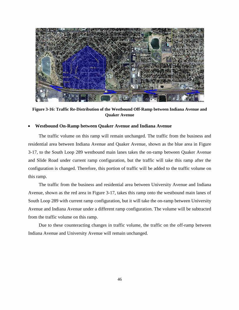
46

Figure 3-16: Traffic Re-Distribution of the Westbound Off-Ramp between Indiana Avenue and

Quaker Avenue

Westbound On-Ramp between Quaker Avenue and Indiana Avenue

The traffic volume on this ramp will remain unchanged. The traffic from the business and

residential area between Indiana Avenue and Quaker Avenue, shown as the blue area in Figure

3-17, to the South Loop 289 westbound main lanes takes the on-ramp between Quaker Avenue

and Slide Road under current ramp configuration, but the traffic will take this ramp after the

configuration is changed. Therefore, this portion of traffic will be added to the traffic volume on

this ramp.

The traffic from the business and residential area between University Avenue and Indiana

Avenue, shown as the red area in Figure 3-17, takes this ramp onto the westbound main lanes of

South Loop 289 with current ramp configuration, but it will take the on-ramp between University

Avenue and Indiana Avenue under a different ramp configuration. The volume will be subtracted

from the traffic volume on this ramp.

Due to these counteracting changes in traffic volume, the traffic on the off-ramp between


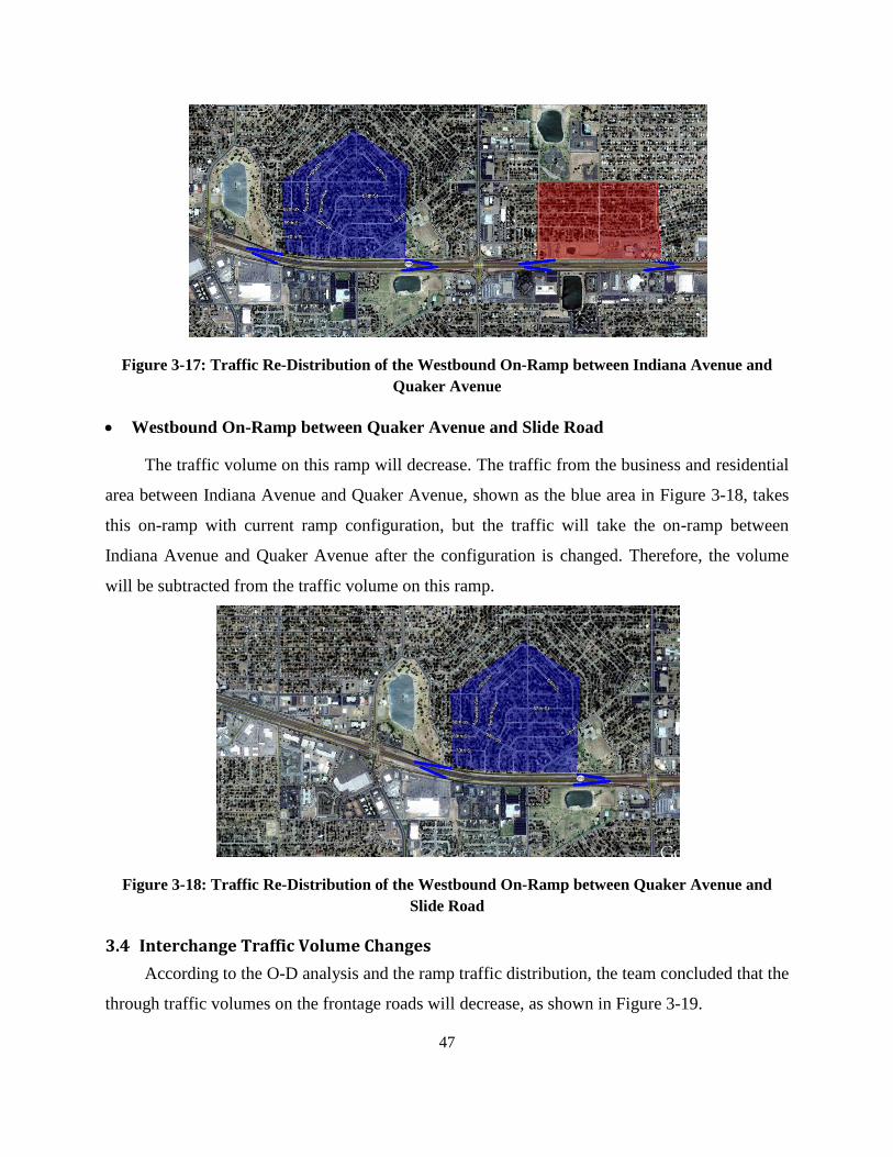
47

Figure 3-17: Traffic Re-Distribution of the Westbound On-Ramp between Indiana Avenue and

Quaker Avenue

Westbound On-Ramp between Quaker Avenue and Slide Road

The traffic volume on this ramp will decrease. The traffic from the business and residential

area between Indiana Avenue and Quaker Avenue, shown as the blue area in Figure 3-18, takes

this on-ramp with current ramp configuration, but the traffic will take the on-ramp between

Indiana Avenue and Quaker Avenue after the configuration is changed. Therefore, the volume

will be subtracted from the traffic volume on this ramp.

Figure 3-18: Traffic Re-Distribution of the Westbound On-Ramp between Quaker Avenue and

Slide Road

3.4 Interchange Traffic Volume Changes

According to the O-D analysis and the ramp traffic distribution, the team concluded that the

through traffic volumes on the frontage roads will decrease, as shown in Figure 3-19.

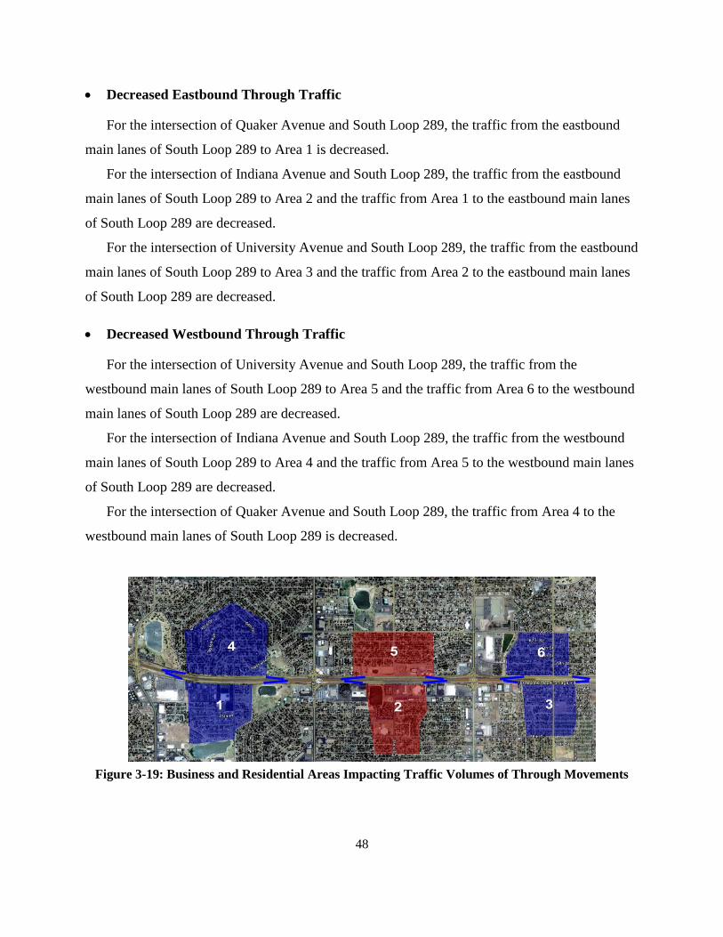
48

Decreased Eastbound Through Traffic

For the intersection of Quaker Avenue and South Loop 289, the traffic from the eastbound

main lanes of South Loop 289 to Area 1 is decreased.

For the intersection of Indiana Avenue and South Loop 289, the traffic from the eastbound

main lanes of South Loop 289 to Area 2 and the traffic from Area 1 to the eastbound main lanes

of South Loop 289 are decreased.

For the intersection of University Avenue and South Loop 289, the traffic from the eastbound

main lanes of South Loop 289 to Area 3 and the traffic from Area 2 to the eastbound main lanes


Decreased Westbound Through Traffic

For the intersection of University Avenue and South Loop 289, the traffic from the

westbound main lanes of South Loop 289 to Area 5 and the traffic from Area 6 to the westbound

main lanes of South Loop 289 are decreased.

For the intersection of Indiana Avenue and South Loop 289, the traffic from the westbound

main lanes of South Loop 289 to Area 4 and the traffic from Area 5 to the westbound main lanes


For the intersection of Quaker Avenue and South Loop 289, the traffic from Area 4 to the

westbound main lanes of South Loop 289 is decreased.

Figure 3-19: Business and Residential Areas Impacting Traffic Volumes of Through Movements

49

3.5

T

raff

ic R

e-R

ou

tin

g R

esu

lts

alo

ng

Fro

nta

ge

Ro

ad

s

Tab

le 3

-1 a

nd T

able

3-2

dem

onst

rate

the

curr

ent

and f

ore

cast

ed t

raff

ic v

olu

me

chan

ges

alo

ng t

he

fronta

ge

road

s of

South

Loop

289,

when

Dia

mond i

nte

rchan

ges

are

chan

ged

to X

-Type

inte

rch

anges

. T

he

red

-mar

ked

cel

ls s

how

the

volu

mes

incr

ease

d b

y t

he

tran

sform

atio

n a

nd t

he

gre

en-m

arked

cel

ls s

how

the

volu

mes

dec

reas

ed b

y t

he

tran

sform

atio

n.

Ta

ble

3-1

: T

raff

ic R

e-R

ou

tin

g a

lon

g F

ron

tage

Road

s of

Sou

th L

oop

289 (

Cu

rren

t T

raff

ic D

ema

nd

)

50

Ta

ble

3-2

: T

raff

ic R

e-R

ou

tin

g a

lon

g F

ron

tage

Road

s of

Sou

th L

oop

289 (

Fore

cast

ed F

utu

re T

raff

ic D

ema

nd

)

51

4. MICROSCOPIC SIMULATION WITH VISSIM AND SYNCHRO

Simulation is a software tool used to replicate the real traffic conditions of the field, to

evaluate operational conditions, and to investigate a transportation network. Microsimulation

models are traffic models used to determine the driving behavior of individual vehicles traveling

on the network. The microsimulation software tools have built-in traffic models for car-

following, lane changing, and gap-acceptance. Microscopic simulation is mainly used for the

evaluation and development of road traffic management and control systems.

Use of microsimulation models provide a better and clearer presentation of actual driver

behavior inside the simulation network. These models are helpful to code complex traffic

problems along with the implementation of intelligent transportation systems. Moreover, these

software packages have an advantage – the ability to show the traffic flow traversing on the

networks and various road and junction types (Bloomberg and Dale, 2000). This helps to

represent the problem and solution in a format understandable to professionals and laymen alike.

VISSIM provides a discrete, stochastic, and time step based microscopic model. In

VISSIM, the driver and the vehicle are modeled as single entities. The traffic flow model in

VISSIM provides a psycho-physical car following model along with the rule-based algorithm for

lane changing movements (Fellendorf and Vortisch, 2005).

VISSIM has a different microscopic simulation model compared to other models in terms

of node-link structure. In VISSIM, networks are modeled based on links and connectors. In this

model, the movement of vehicles is controlled by the node-link structure, in which the vehicle

after arriving to the end of a link depends on the upstream or downstream node above or below

to continue its trajectory (Gonzalez, 2006).

4.1 Network Coding

The study area consists of a freeway section with four major interchanges connected by

frontage roads in both eastbound and westbound directions. The VISSIM microsimulation model

was used for the development of the network of the corridor. The network was constructed using

a 2D environment and then converted into 3D mode by assigning an elevation (arbitrary) to the

links and connectors to provide a 3D view to the network.

52

VISSIM

The roadway network was designed in VISSIM using the details obtained from Google

Earth. The network geometry was then checked against the “Sign and Striping Layout” provided

by the Texas Department of Transportation (TxDOT) Lubbock District and also against the

geometry observed in the field from the visits made to the project area. The network was

designed on the background image, obtained from Google Earth, which had to be scaled to the

real world dimensions. The area of interest is a five-mile portion, starting from IH-27 and

extending to Spur 329 as shown in Figure 4-1.

Figure 4-1: Google Earth Image of the Project Area

The network was developed using links and connectors. After the whole network had been

modeled, the geometric design was checked to verify the accuracy of the length of the curves,

ramps, distance between the two intersections of the interchange, number of lanes, width of the

lanes, etc. After the roadway network was modeled, traffic control systems (e.g., signal, stop, and

yield controls, etc.), and total volume inputs were coded throughout the network.

The signal controller was designed as a fixed time controller for all the intersections and

the signal timing data was collected for all the intersections. The volume inputs were obtained

from the raw data files provided by the Lubbock District TxDOT office. The simulation was run

with the original volume and signal timing plan. The sample snapshots of the network coding

and the simulations are shown in Figure 4-2 and in Figure 4-3.

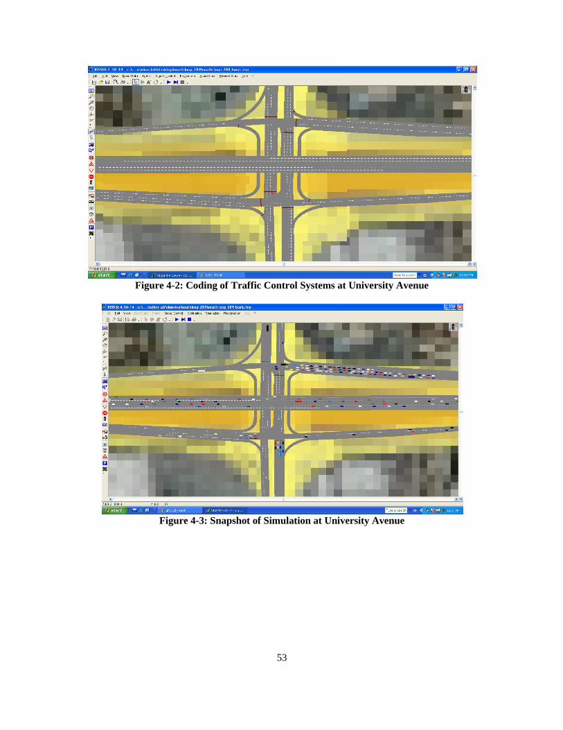
53

Figure 4-2: Coding of Traffic Control Systems at University Avenue

Figure 4-3: Snapshot of Simulation at University Avenue

54

Synchro

The Synchro simulation model was used for the development of the network. The network

was designed on the background image, obtained from Google Earth, and scaled to the real

world dimensions. The network was developed using links and nodes. After the roadway

network, traffic volume inputs were coded throughout the network. This included main lanes,

frontage roads, on-ramps and off-ramps, as well as intersection volumes.

Figure 4-4: Screen Shot of the Synchro Model

At all interchanges, volumes were taken at each movement on an individual lane basis for the

major arterial and frontage road intersection. This resulted in a large amount of data being

recorded in 15 minute intervals for several days. For each movement a Peak Hour Factor (PHF)

was determined and then a conservative hourly volume was formed. This was also repeated for

each ramp throughout the study area.

The signal phase orders, green times, and cycle lengths were adopted from the City of

Lubbock Traffic Engineering Department designs for all the intersections, including Slide,

Quaker, Indiana, and University. The design was performed as a traditional TTI-4-Phase

operation. A 130-second cycle length was used as the coordination cycle length for peak hours in

55

accordance with the City of Lubbock local traffic engineering department. An average four

second yellow time and a two second all-red time were used for each phase

The volume inputs were obtained from the raw data files provided by the Lubbock District

TxDOT office. The simulation was run with the current and forecasted volumes. The signal

timing plan was adopted from the City of Lubbock traffic engineering department. The sample

snapshots of the network coding and the simulations are shown in Figures 4-5 and 4-6.

Figure 4-5: Coding of Traffic Control System at University Avenue

56

Figure 4-6: Snapshot of Simulation at University Avenue

4.2 Model Calibration and Validation

Validation and calibration were required to gauge the accuracy of the simulation. Phase II

simulations were calibrated in a similar manner as done in Phase I. This method required taking

cuts at sections, recording the traffic volumes in the simulation, and comparing the results to the

measured field volumes to verify statistical accuracy.

The simulation model was validated after each pass of simulation and checked for validity

using two statistic tests: Correlation Coefficient and Root Mean Squared-Error (RMSE). The two

tests were conducted on the original traffic volume obtained from field observation and the

volume obtained from the simulation output.

The correlation coefficient ( ) indicates how closely the model-predicted data matches the

observed data. Its value lies between 0 and 1. A correlation coefficient value closer to 1 is

desirable. The formula for the term is (Ambadipudi and Dorothy, 2006):

2

2222

2

))()()((

))((

i ii iiii i

i ii ii ii

CountCountnVolumeVolumen

VolumeCountVolumeCountnr

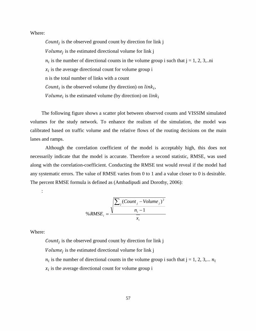
57

Where:

is the observed ground count by direction for link j

is the estimated directional volume for link j

is the number of directional counts in the volume group i such that j = 1, 2, 3,..ni

is the average directional count for volume group i

n is the total number of links with a count

is the observed volume (by direction) on ,

is the estimated volume (by direction) on

The following figure shows a scatter plot between observed counts and VISSIM simulated

volumes for the study network. To enhance the realism of the simulation, the model was

calibrated based on traffic volume and the relative flows of the routing decisions on the main

lanes and ramps.

Although the correlation coefficient of the model is acceptably high, this does not

necessarily indicate that the model is accurate. Therefore a second statistic, RMSE, was used

along with the correlation-coefficient. Conducting the RMSE test would reveal if the model had

any systematic errors. The value of RMSE varies from 0 to 1 and a value closer to 0 is desirable.

The percent RMSE formula is defined as (Ambadipudi and Dorothy, 2006):

:

i

i

j jj

ix

n

VolumeCount

RMSE1

)(

%

2

Where:

is the observed ground count by direction for link j

is the estimated directional volume for link j

is the number of directional counts in the volume group i such that j = 1, 2, 3,...

is the average directional count for volume group i

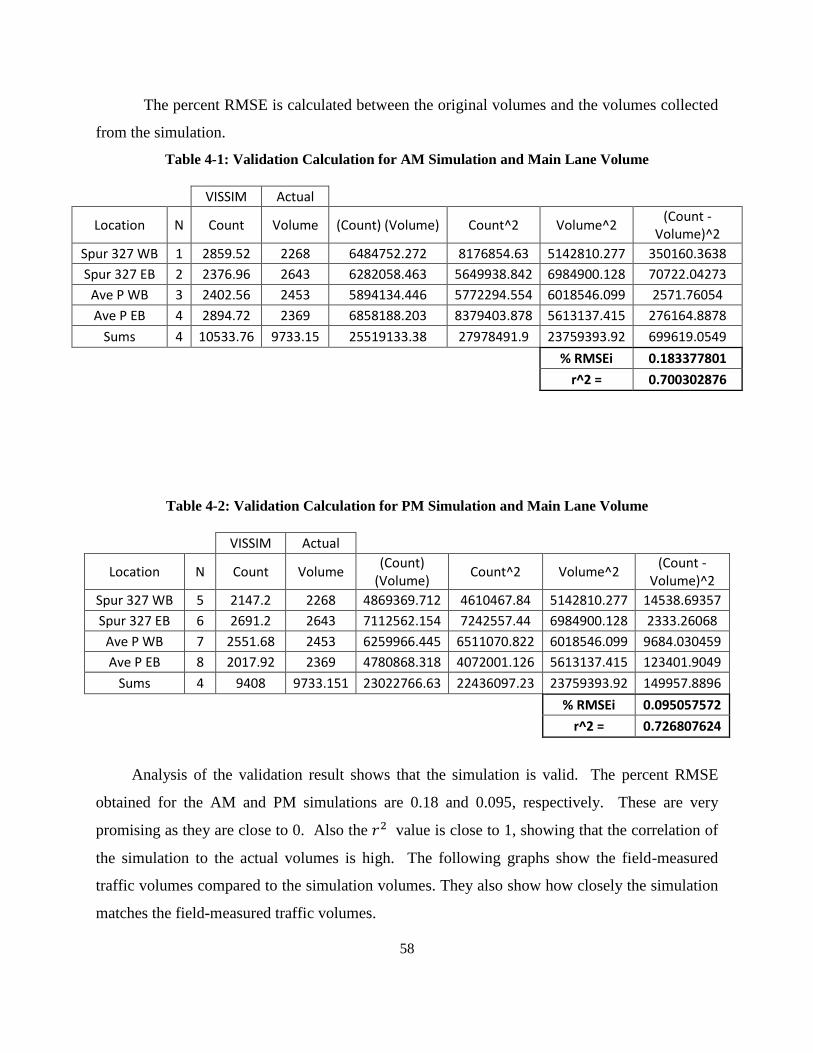
58

The percent RMSE is calculated between the original volumes and the volumes collected

from the simulation.

Table 4-1: Validation Calculation for AM Simulation and Main Lane Volume

VISSIM Actual

Location N Count Volume (Count) (Volume) Count^2 Volume^2 (Count -

Volume)^2

Spur 327 WB 1 2859.52 2268 6484752.272 8176854.63 5142810.277 350160.3638

Spur 327 EB 2 2376.96 2643 6282058.463 5649938.842 6984900.128 70722.04273

Ave P WB 3 2402.56 2453 5894134.446 5772294.554 6018546.099 2571.76054

Ave P EB 4 2894.72 2369 6858188.203 8379403.878 5613137.415 276164.8878

Sums 4 10533.76 9733.15 25519133.38 27978491.9 23759393.92 699619.0549

% RMSEi 0.183377801

r^2 = 0.700302876

Table 4-2: Validation Calculation for PM Simulation and Main Lane Volume

VISSIM Actual

Location N Count Volume (Count)

(Volume) Count^2 Volume^2

(Count - Volume)^2

Spur 327 WB 5 2147.2 2268 4869369.712 4610467.84 5142810.277 14538.69357

Spur 327 EB 6 2691.2 2643 7112562.154 7242557.44 6984900.128 2333.26068

Ave P WB 7 2551.68 2453 6259966.445 6511070.822 6018546.099 9684.030459

Ave P EB 8 2017.92 2369 4780868.318 4072001.126 5613137.415 123401.9049

Sums 4 9408 9733.151 23022766.63 22436097.23 23759393.92 149957.8896

% RMSEi 0.095057572

r^2 = 0.726807624

Analysis of the validation result shows that the simulation is valid. The percent RMSE

obtained for the AM and PM simulations are 0.18 and 0.095, respectively. These are very

promising as they are close to 0. Also the value is close to 1, showing that the correlation of

the simulation to the actual volumes is high. The following graphs show the field-measured

traffic volumes compared to the simulation volumes. They also show how closely the simulation

matches the field-measured traffic volumes.

59

Figure 4-7: AM Comparison of Actual to Simulation Volumes

Figure 4-8: PM Comparison of Actual to Simulation Volumes

0

500

1000

1500

2000

2500

3000

3500

Spur 327 WB Spur 327 EB Ave P WB Ave P EB

VISSIM Actual

0

500

1000

1500

2000

2500

3000

Spur 327 WB Spur 327 EB Ave P WB Ave P EB

VISSIM Actual

60

5. LEVEL OF SERVICE ANALYSIS OF MAIN LANES AND FRONTAGE

ROADS

This section presents the analysis on the LOS on the main lanes and frontage roads of

South Loop 289 for morning and afternoon peak hours regarding the current as well as future

traffic conditions. The research area consists of five major interchanges: Slide Road, Quaker

Avenue, Indiana Avenue, University Avenue and IH-27. At present, Indiana Avenue and

University Avenue have Diamond interchanges, Slide Road has an X pattern interchange, and

the ramp configuration changes from X to Diamond at Quaker Avenue.

For the frontage road, the analysis focuses on the sections between the five major

intersections, particularly between the on- and off-ramp segments as shown in Figure 5.1. For

main lane traffic, the analysis is conducted at five different sections in both eastbound and

westbound directions as shown in Figure 5-2.

Figure 5-1: Four Frontage Road Sections on the Network where the LOS Analysis was Conducted

61

Figure 5-2: Five Main Lane Sections on the Network Where the LOS Analysis was Conducted

The analysis aims to evaluate the potential impacts of the improvement alternatives on both

freeway main lanes and frontage roads. As the traffic on the frontage road is highly interrupted

by the on- and off-ramps as well as the intersections, the profile of the speed and density along

the frontage road is highly variable. The V/C ratio was thus selected as the performance indicator

for evaluating the LOS on the frontage road. The detailed simulation results of the three

improvement alternatives in terms of the traffic volume, V/C ratio, density, and LOS are

presented section by section. Only the results from the westbound traffic are used for illustrative

purposes, because the changes on the eastbound as a result of these improvement strategies are

likely to be the same.

5.1 Current Condition

The current level of service (LOS) on the main lanes and frontage roads of the corridor

were evaluated for both morning and afternoon peak hours. Simulation results revealed that the

LOS for main lane traffic in both morning and afternoon peak hours ranges from ‘B’ to ‘D’,

while the LOS for the frontage roads ranges from ‘B’ to ‘C’. For illustrative purposes, the effects

of the improvement alternatives on the westbound direction of the corridor are presented in this

section.

Frontage road between Slide Road and Quaker Avenue (FS1)

Frontage road between Quaker Avenue and Indiana Avenue (FS2)

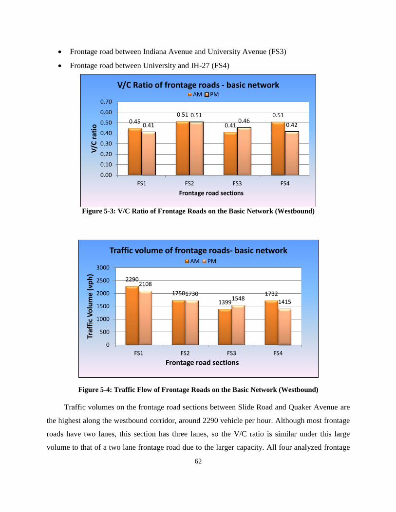
62

Frontage road between Indiana Avenue and University Avenue (FS3)

Frontage road between University and IH-27 (FS4)

Figure 5-3: V/C Ratio of Frontage Roads on the Basic Network (Westbound)

Figure 5-4: Traffic Flow of Frontage Roads on the Basic Network (Westbound)

Traffic volumes on the frontage road sections between Slide Road and Quaker Avenue are

the highest along the westbound corridor, around 2290 vehicle per hour. Although most frontage

roads have two lanes, this section has three lanes, so the V/C ratio is similar under this large

volume to that of a two lane frontage road due to the larger capacity. All four analyzed frontage

0.45 0.51

0.41

0.51

0.41

0.51 0.46

0.42

0.00

0.10

0.20

0.30

0.40

0.50

0.60

0.70

FS1 FS2 FS3 FS4

V/C

rat

io

Frontage road sections

V/C Ratio of frontage roads - basic network AM PM

2290

1750

1399

1732

2108

1730 1548

1415

0

500

1000

1500

2000

2500

3000

FS1 FS2 FS3 FS4

Traf

fic

Vo

lum

e (v

ph

)


Traffic volume of frontage roads- basic network AM PM

63

road sections are not at capacity. Except for the frontage road between Indiana and University

Avenue, the traffic volumes are higher in the morning peak hours than the afternoon peak hours.

The current traffic condition on main lane traffic in terms of total traffic volume on the

westbound is illustrated in Figure 5-5. The values on the Y-axis represent the traffic volume in

vehicle per hour, while the labels on the X-axis represent the five sections of the network as

follows:

Slide Road overpass (S1)

Slide Road and Quaker Avenue (S2)

Quaker Avenue and Indiana Avenue (S3)

Indiana Avenue and University Avenue (S4)

University Avenue and IH-27 (S5).

Figure 5-5: Traffic Volumes on Main Lane Segments on the Basic Network (Westbound)

The highest traffic volume along the westbound corridor occurs on the freeway section

between Quaker Avenue and Indiana Avenue, amounting to 3977 and 4707 vehicle per hour for

morning and afternoon peak hours, respectively. This is shown in the density profile of Figure

5-6. The most congested section lies between Quaker Avenue and Indiana Avenue, the density of

which reaches 29 vehicles per mile per lane. However, with current traffic demand, none of the

segments on the freeway and frontage roads has reached its capacity.

3876

2596

3977 3846

3025

3179

2228

4707

3940

3238

0

1000

2000

3000

4000

5000

MS1 MS2 MS3 MS4 MS5

Traf

fic

Vo

lum

e (v

ph

)

Mainlane Sections

Mainlane Traffic Volume - Basic Network

AM PM

64

Figure 5-6: Traffic Densities of Main lane Segments on the Basic Network (Westbound)

5.2 Section by Section Evaluation on the Frontage Roads of the Improvement

Alternatives

As implied in the Phase I study, though the alternatives to a certain degree improve the

LOS on the freeway segments, they may impact the traffic distribution between the main lane

and frontage roads. Particularly, with reconfiguration from Diamond to X type interchanges, a

certain amount of traffic will be directed onto the frontage roads, which results in an increase of

traffic volume and weaving behavior. In this section, LOS analysis was conducted to evaluate the

impact the three alternatives have on the frontage roads. The corresponding traffic densities on

the freeway main lanes are also presented to illustrate the traffic redistribution, as shown in the

Phase I report.

Effects of Different Alternatives on Frontage Road Section 1: Between Slide Road

and Quaker Avenue

The simulation results reflecting the effects of Alternative 1 (A1), Alternative 2 (A2), and

Alternative 3 (A3) on traffic volumes on the frontage road between Slide Road and Quaker

Avenue (FS1) is shown in Figure 5-7. The labels on the X-axis represent the alternative networks

and each column on the X-axis shows the number of vehicles traveling on that frontage road

segment for each alternative.

22

14

22 21 17 18

13

29

22 18

0

5

10

15

20

25

30

35

MS1 MS2 MS3 MS4 MS5

Traf

fic

Den

sity

(vp

m)

Mainlane Sections

Mainlane Traffic Density- Basic Network

AM PM

65

Since the interchange of Slide Road, as well as the westbound direction of the interchange

of Quaker Avenue, was already an X-type interchange, Alternative 2 does not change the traffic

distribution on this segment. Therefore, the traffic volumes for both AM and PM peak hours

almost remain the same. Similar results were also obtained under Alternatives 1 and 3. The slight

differences in the traffic volumes for these alternatives are mostly attributed to the stochastic

traffic variations in VISSIM simulation.

Figure 5-7: Traffic Volume on the Section FS1 for Differnet Alternatives

Figure 5-8 illustrates the changes in terms of the V/C ratio at the frontage road between

Slide and Quaker regarding different improvement strategies. The results are easy to understand

since the V/C ratio is proportional to the traffic volume. All three alternatives do not have

notable impacts on this frontage road segment, thus the V/C ratio as well as the LOS remains

unchanged.

2290 2217 2242 2205 2108 2142 2067 2151

0

500

1000

1500

2000

2500

3000

BN A2 A1 A3

Traf

fic

Vo

lum

e (v

ph

)


Traffic Volume of Frontage Road between Slide and Quaker for Different Alternatives

AM PM

66

Figure 5-8: V/C Ratio on the Section FS1 for Different Alternatives

The following two figures present the main lane traffic densities on the Slide overpass

and the segement between Slide Road and Quaker Avenue. Consistent conclusions with the

Phase 1 study can be drawn. For the Slide overpass, adding an auxiluary lane in both Alternative

1 and Alternative 3 will decrease the density due to the increase in capacity. Alternative 2 does

not change the interchange configuration of Slide Road, so it does not significantly reduce the

traffic density on the Slide overpass. For the freeway segment between Slide Road and Quaker

Avenue, none of the three alternatives will directly impact the traffic distribution or the segment

capacity as analyzed in Phase 1; the density for this segment remains almost the same for each

alternative.

0.45 0.43 0.44 0.43 0.41 0.42 0.41 0.42

0.00

0.10

0.20

0.30

0.40

0.50

0.60

0.70

BN A2 A1 A3

V/C

rat

io

Simulation networks

V/C Ratios of Frontage Road between Slide and Quaker for Different Alternatieves

AM PM

67

Figure 5-9: Traffic Density on the Freeway Section MS1 for Different Alternatives

Figure 5-10: Traffic Density on the Freeway Section MS2 for Different Alternatives

Effects of the Alternatives on Frontage Road Section 2: Quaker Avenue and Indiana

Avenue

The second analyzed frontage road section is between Quaker Avenue and Indiana

Avenue. The conversion of Quaker Avenue and Indiana Avenue from Diamond to X type will

22 21

15 16 18 17

14 13

0

5

10

15

20

25

30

BN A2 A1 A3

Traf

fic

Den

sity

(vp

m)

Simulation networks

Traffic Densities of Slide Overpass for Different Alternatieves

AM PM

14 14 15

14 13 13 13

12

0

5

10

15

20

BN A2 A1 A3

Traf

fic

De

nsi

ty (

vpm

)

Simulation networks

Traffic Densities of Mainlanes between Slide and Quaker for Different Alternatieves

AM PM

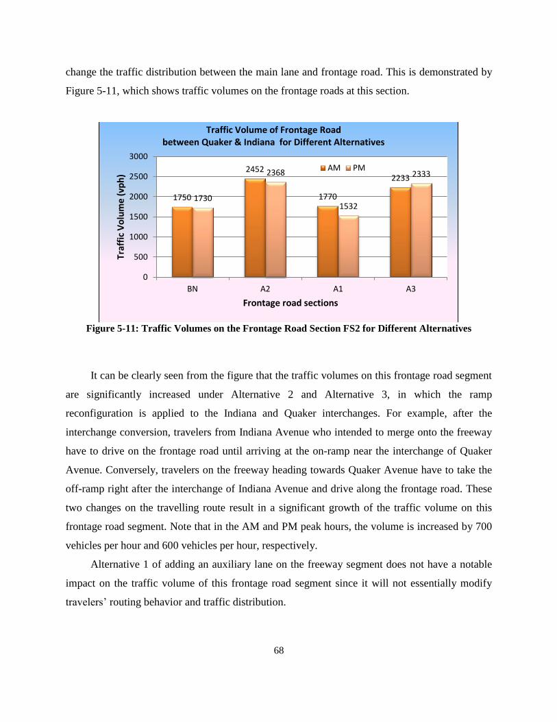
68

change the traffic distribution between the main lane and frontage road. This is demonstrated by

Figure 5-11, which shows traffic volumes on the frontage roads at this section.

Figure 5-11: Traffic Volumes on the Frontage Road Section FS2 for Different Alternatives

It can be clearly seen from the figure that the traffic volumes on this frontage road segment

are significantly increased under Alternative 2 and Alternative 3, in which the ramp

reconfiguration is applied to the Indiana and Quaker interchanges. For example, after the

interchange conversion, travelers from Indiana Avenue who intended to merge onto the freeway

have to drive on the frontage road until arriving at the on-ramp near the interchange of Quaker

Avenue. Conversely, travelers on the freeway heading towards Quaker Avenue have to take the

off-ramp right after the interchange of Indiana Avenue and drive along the frontage road. These

two changes on the travelling route result in a significant growth of the traffic volume on this

frontage road segment. Note that in the AM and PM peak hours, the volume is increased by 700

vehicles per hour and 600 vehicles per hour, respectively.

Alternative 1 of adding an auxiliary lane on the freeway segment does not have a notable

impact on the traffic volume of this frontage road segment since it will not essentially modify

travelers’ routing behavior and traffic distribution.

1750

2452

1770

2233

1730

2368

1532

2333

0

500

1000

1500

2000

2500

3000

BN A2 A1 A3

Traf

fic

Vo

lum

e (

vph

)


Traffic Volume of Frontage Road between Quaker & Indiana for Different Alternatives

AM PM

69

In terms of the V/C ratio, the increased traffic volume on the frontage road for A2 and A3

can be well accommodated by adding an auxiliary lane on the frontage road as shown in Figure

5-12. The highest V/C ratio of 0.51 occurs under Alternative 1 for the morning peak, which is

almost the same as that in the basic network. All three alternatives enable the LOS on this

frontage road segment to remain in an under-saturated category of ‘C’.


Figure 5-13 depicts the traffic densities on the corresponding main lane segment between

Quaker Avenue and Indiana Aveue. This chart shows that traffic densities from all three

alternatives are significantly reduced compared with the basic network. However, this reduction

is achieved in different ways. Alternative 2 and Alternative 3 reduced the traffic on the freeway

segment by diverting to a frontage road, while the improvement of Alternative 1 is achieved

through increasing the capacity by adding an additional lane.

0.51 0.48

0.52

0.44 0.51

0.46 0.45 0.46

0.00

0.20

0.40

0.60

BN A2 A1 A3

V/C

rat

io

Simulation networks

V/C Ratios of Frontage Road between Quaker & Indiana for Different Alternatieves

AM PM

70

Figure 5-13: Traffic Densities on the Freeway Section MS3 for Different Alternatives

Effects of the Alternatives on Frontage Road Section 3: Indiana Avenue and

University Avenue

Similar to the frontage road section between Quaker Avenue and Indiana Avenue, the

conversion of interchanges on both Indiana Avenue and University Avenue will result in a

redistribution of traffic between frontage roads and freeway main lanes. The traffic volumes on

the frontage road are expected to increase, as illustrated by the simulation results in Figure 5-14.

It can be seen that both Alternative 2 and Alternative 3 will significantly increase the traffic

volumes on the frontage roads. For example, the total traffic volume on the frontage road of the

basic network during the morning peak hours is 1399 vehicles per hour. This is increased by

almost 50%, to 2094, in the case of Alternative 2. The traffic volume caused by Alternative 3 is

similar to that of Alternative 2, due to the similar trip distribution along the corridor.

22

17 18 15

29

22 22 21

0

5

10

15

20

25

30

35

BN A2 A1 A3

Traf

fic

De

nsi

ty (

vpm

)

Simulation networks

Traffic Densities of Mainlanes between Quaker and Indiana Ave. for Different Alternatieves

AM PM

71


In terms of V/C ratio, the three alternatives achieve very close peformances compared with

the basic network. For alternatives A2 and A3, adding an auxiliary lane on the frontage road

directly increased the capcity, which can well accomondate the increase in traffic volume. For

A1, the result is also obvious since adding an auxiliary lane on the freeway segment will not

significnatly change the traffic volume or the V/C ratio on the frontage road.


1399

2094

1456

2140

1548

2184

1398

2188

0

500

1000

1500

2000

2500

3000

BN A2 A1 A3

Traf

fic

Vo

lum

e (

vph

)


Traffic Volume of Frontage Road between Indiana & Univ. for Different Alternatives

AM PM

0.41 0.41 0.43 0.42 0.46 0.43 0.41 0.43

0.00

0.10

0.20

0.30

0.40

0.50

0.60

0.70

BN A2 A1 A3

V/C

rat

io

Simulation networks

V/C Ratios of Frontage Road between Indiana & Univ. for Different Alternatieves

AM PM

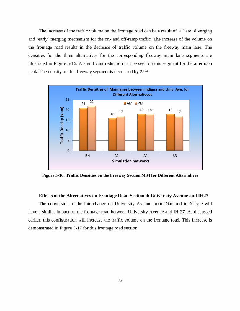
72

The increase of the traffic volume on the frontage road can be a result of a ‘late’ diverging

and ‘early’ merging mechanism for the on- and off-ramp traffic. The increase of the volume on

the frontage road results in the decrease of traffic volume on the freeway main lane. The

densities for the three alternatives for the corresponding freeway main lane segments are

illustrated in Figure 5-16. A significant reduction can be seen on this segment for the afternoon

peak. The density on this freeway segment is decreased by 25%.


Effects of the Alternatives on Frontage Road Section 4: University Avenue and IH27

The conversion of the interchange on University Avenue from Diamond to X type will

have a similar impact on the frontage road between University Avenue and IH-27. As discussed

earlier, this configuration will increase the traffic volume on the frontage road. This increase is

demonstrated in Figure 5-17 for this frontage road section.

21

16 18 18

22

17 18

17

0

5

10

15

20

25

BN A2 A1 A3

Traf

fic

De

nsi

ty (

vpm

)

Simulation networks

Traffic Densities of Mainlanes between Indiana and Univ. Ave. for Different Alternatieves

AM PM

73


As shown in Figure 5-17, the traffic volume on this frontage road segment is significantly

increased by 800 vehicles per hour and 900 vehicles per hour for the morning and afternoon peak

hours, respectively. However, the increased traffic volume is compensated by the auxiliary lane

added onto the frontage road. So in terms of the V/C ratio, the performance does not have a

significant growth, and remains at the level of ‘C’.

Figure 5-18: V/C Ratio on the Frontage Road Section FS4 for Different Alternatives

A similar impact on the main lane traffic for the three alternatives is also obtained as

illustrated in Figure 5-19. The traffic density of the main lane traffic is improved by all three

1732

2504

1745

2748

1415

2384

1566

2451

0

500

1000

1500

2000

2500

3000

BN A2 A1 A3

Traf

fic

Vo

lum

e (

vph

)


Traffic Volume of Frontage Road between Univ. Ave. and IH27 for Different Alternatives

AM PM

0.51 0.49 0.51 0.54

0.42 0.47 0.46 0.48

0.00

0.20

0.40

0.60

BN A2 A1 A3

V/C

rat

io

Simulation networks

V/C Ratios of Frontage Road between Univ. & IH27 for Different Alternatieves

AM PM

74

strategies. Alternative 1 achieves this by increasing the capacity. But for Alternatives 2 and 3,

this improvement is due to distributing a certain amount of traffic onto the frontage roads.


5.3 Summary for the Current Condition

In the previous section, the impact of the three alternatives was illustrated section by

section along the westbound corridor of South Loop 289. This section summarizes the simulation

results and LOS on both the east and westbound sections. The LOS for both frontage roads and

mainlanes in the basic network is listed in Table 5-2.

17

13 13 12

18

15 14 14

0

5

10

15

20

25

BN A2 A1 A3

Traf

fic

De

nsi

ty (

vpm

)

Simulation networks

Traffic Densities of Mainlanes between Univ. Ave and IH27 for Different Alternatieves

AM PM

75

Table 5-1: LOS of Traffic on Frontage Roads and Main Lanes of Basic Network

Basic Network

AM PM

Frontage Roads

Slide Road & Quaker Ave. Westbound C C

Eastbound C C

Quaker & Indiana Westbound C C

Eastbound C C

Indiana & University Westbound B B

Eastbound C C

University & I-27 Westbound C C

Eastbound C C

Main lanes

Slide Road & Quaker Ave. Westbound B B

Eastbound B B

Quaker & Indiana Westbound C D

Eastbound C C

Indiana & University Westbound C C

Eastbound C C

University & I-27 Westbound B B

Eastbound C B

For Alternative 1, adding an auxiliary lane does not have a direct impact on the LOS on

the frontage roads. The only two changes of LOS on the frontage road sections (westbound

between Indiana Avenue and University Avenue, westbound betweeen University and I-27) is

due to the stochastic flutuation of traffic volume in the simualtion software and the V/C ratio is

at the edge between grades ‘B’ and ‘C’. Consistent with the analysis using 2007 traffic volume,

the LOS on the freeway main lanes is improved by adding an extra lane. However, the lane

distirbution on the main lanes is uneven and results in high traffic volume on the outside lane,

which still remains at a high level of traffic density, as well as producing weaving maneuvers.

76

Table 5-2: Comparison of LOS between Basic Network and Alternative 1

AM PM

Basic

Network

A1 Basic

Network

A1

Frontage Roads

Slide Road & Quaker Ave. Westbound C

C B B

Eastbound C C C C

Quaker & Indiana Westbound C

C C C

Eastbound C C C C

Indiana & University Westbound B

B C B

Eastbound C C C C

University & I-27 Westbound C

C B C

Eastbound C C C C

Main laneMain lanes

Slide Road & Quaker Ave. Westbound B B B B

Eastbound B B B B

Quaker & Indiana Westbound C B D C

Eastbound C C C B

Indiana & University Westbound C B C C

Eastbound C B C B

University & I-27 Westbound B B B B

Eastbound C B B B

Alternative 2 converts interchanges along the corridor from Diamond to X type, which

leads to a redistributed traffic pattern between frontage roads and main lanes. Specifically, a

certain amount of travellers with short O-D trips will be shifted from the freeway to the frontage

road. This results in an increase of traffic volume on the frontage road; however, this is

compensated by adding an auxiliary lane on the frontage road between the on- and off-ramps.

The changes of LOS on the frontage road are very limited as illustrated in Table 5-3.

77


AM PM

Basic

Network

A2 Basic

Network

A2

Frontage Roads

Slide Road & Quaker Ave. Westbound C

C B B

Eastbound C C C C


C C C

Eastbound C C C C

Indiana & University Westbound B

B C B

Eastbound C C C C

University & I-27 Westbound C

C B C

Eastbound C C C C

Main lanes

Slide Road & Quaker Ave. Westbound B

B B

B

Eastbound B B

B B


C D

C

Eastbound C B

C C

Indiana & University Westbound C

B C

C

Eastbound C C

C B

University & I-27 Westbound B

B B

B

Eastbound C B

B B

Alternative 3 further supplements Alternative 2 by adding an auxiliary lane on the

overpass of each interchange (between on- and off-ramps) to further relieve the traffic on the

freeway main lanes. It is easy to see that this auxiilary lane has little impact on the frontage roads

or the freeway segments between the interchanges. However, it is expected that the traffic on the

overpass of each interchange will be improved since the capacities are increased.

78


AM PM

Basic

Network

A3 Basic

Network

A3

Frontage Roads

Slide Road & Quaker Ave. Westbound C C B B

Eastbound C C C C

Quaker & Indiana Westbound C C C C

Eastbound C C C C

Indiana & University Westbound B B C B

Eastbound C C C C

University & I-27 Westbound C C B C

Eastbound C C C C

Main lanes


Eastbound B B B B

Quaker & Indiana Westbound C B D C

Eastbound C B C B

Indiana & University Westbound C B C B

Eastbound C B C B


Eastbound C B B B

In comparison, Alternative 2 achieves almost the same performance as Alternative 1 by

converting the ramp configurations from Diamond to X pattern at interchanges. As demonstrated

in the Phase 1 study, Alternative 2 also has an advantage that the traffic across different main

lanes is more evenly distributed when compared to Alternative 1.

The results demonstrated that the traffic on the frontage roads is significantly increased

under Alternative 2; however, this increase can be well accommodated by adding an auxiliary

lane on the frontage road, allowing the LOS on the frontage road to remain almost unchanged.

Alternative 3 further supplements Alternative 2 by adding an auxiliary lane on the overpass

of each interchange, which will increase the capacity of the main lane segments between on- and

79

off-ramps. However, A3 does not create significant improvement compared to Alternative 2 and

is not necessary at this stage. Hence Alternative 2, which changes the ramp configuration from

Diamond to X type with an auxiliary lane added onto the frontage road, is recommended.

5.4 LOS Analysis for the Projected Traffic

The traffic projection is conducted on the basis of a 3% annual increase for five years for

South Loop 289. This traffic growth rate was estimated by considering the actual traffic growth

counted on the South Loop main lanes in 2008, 2009, and 2010 and verified by the transportation

planning process calculations. The potential effects of the proposed improvement alternatives on

LOS on the frontage roads are analyzed similarly to the analysis of current conditions.

Basic Network

The analysis was first conducted on the basic network without any modifications in

roadway geometry. Changes in traffic density and volume on the main lanes along South Loop

289 are illustrated in Figure 5-20. As shown, the traffic volume was significantly increased by

an amount ranging from 300 to 700 vehicles per hour. The densities were also higher compared

to current traffic conditions. The most congested section appears to be the segment between

Quaker Avenue and Indiana Avenue, for which the density reached 34 vehicles per mile per lane,

which is very close to LOS ‘E’ (35 vehicles per mile per lane). The growth of traffic demand

resulted in the LOS of some segments changing from ‘C’ to ‘D’ as listed in Table 5-5.

4477

2998

4593 4442

3494

3672

2573

5437

4551

3740

0

1000

2000

3000

4000

5000

6000

MS1 MS2 MS3 MS4 MS5

Traf

fic

Vo

lum

e (

vph

)

Mainlane Sections

Mainlane Traffic Volume - Basic Network

AM PM

Figure 5-20: Traffic Volume on Main Lane Distribution on the Basic Network under Forecasted Traffic

Conditions in 2016 (Westbound)

80

Figure 5-21: Traffic Densities on the Main Lanes of the Basic Network under Forecasted Traffic


Similarly, for the current network configuration, the traffic flow as well as the V/C ratio

will also significantly increase on the frontage roads. Several segments reached a V/C ratio of

0.59, which is very close to LOS ‘D’ (0.62). This increase results in the LOS on some segments

of the frontage road, degrading from level ‘B’ to ‘C.’

25

16

25 24

20 21

15

33

25

21

0

5

10

15

20

25

30

35

40

MS1 MS2 MS3 MS4 MS5

Traf

fic

De

nsi

ty (

vpm

)

Mainlane Sections

Mainlane Traffic Density- Basic Network

AM PM

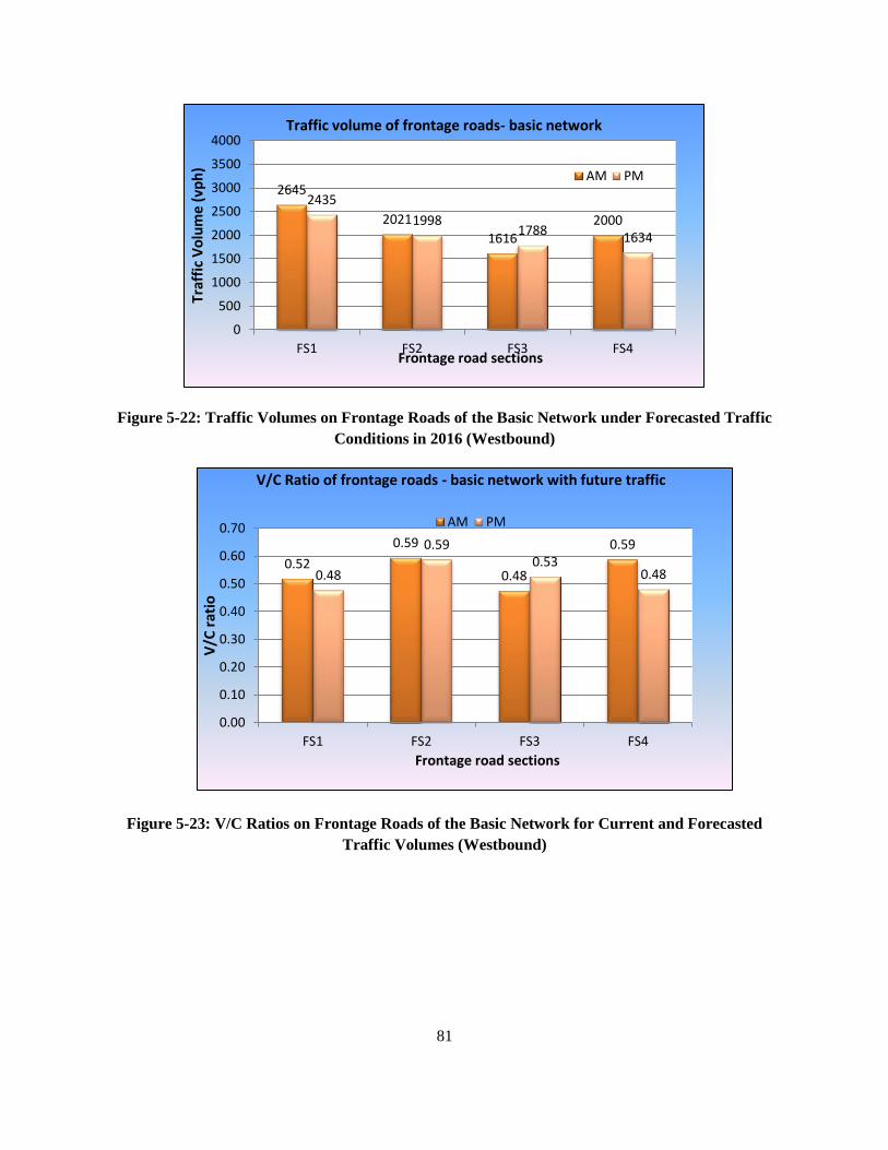
81

Figure 5-22: Traffic Volumes on Frontage Roads of the Basic Network under Forecasted Traffic


Figure 5-23: V/C Ratios on Frontage Roads of the Basic Network for Current and Forecasted

Traffic Volumes (Westbound)

2645

2021

1616

2000

2435

1998 1788

1634

0

500

1000

1500

2000

2500

3000

3500

4000

FS1 FS2 FS3 FS4

Traf

fic

Vo

lum

e (

vph

)


Traffic volume of frontage roads- basic network

AM PM

0.52

0.59

0.48

0.59

0.48

0.59 0.53

0.48

0.00

0.10

0.20

0.30

0.40

0.50

0.60

0.70

FS1 FS2 FS3 FS4

V/C

rat

io


V/C Ratio of frontage roads - basic network with future traffic

AM PM

82

Table 5-5: Comparison of LOS in the Basic Network between Current and Future Traffic

Conditions

AM PM

Current Future Current Future

Frontage Roads

Slide Road & Quaker Ave. Westbound C C B C

Eastbound C C C C


Eastbound C D C D

Indiana & University Westbound B C C C

Eastbound C C C C

University & I-27 Westbound C C B C

Eastbound C C C C

Main lanes


Eastbound B C B C

Quaker & Indiana Westbound C C D D

Eastbound C D C D

Indiana & University Westbound C C C C

Eastbound C D C D

University & I-27 Westbound B C B C

Eastbound C C B C

Alternative 1

The V/C ratios of the frontage road sections with projected traffic volumes are illustrated in

Figure 5-24. Compared with the current traffic conditions, the frontage road segment between

Slide Road and Quaker Avenue and the segment between Indiana Avenue and University

Avenue have been degraded from ‘B’ to ‘C’.

83


(Westbound)

Figure 5.25 further illustrates the LOS on the main lanes for the projected traffic

conditions compared to the current situation. The densities of all the main lane traffic increase.

For example, the freeway segment between Indiana Avenue and University Avenue degraded

from ‘B’ to ‘C’ for both morning and afternoon peak hours.

Figure 5-25: Effect of Alternative 1 on Main Lane with Current and Projected Traffic Data

(Westbound)

0.44

0.52

0.43

0.51

0.41 0.45

0.41 0.46

0.00

0.20

0.40

0.60

FS1 FS2 FS3 FS4

V/C

rat

io


V/C Ratio of frontage roads of A1 for current traffic

AM PM

0.49

0.60

0.49

0.59

0.47 0.52

0.47 0.53

0.00

0.20

0.40

0.60

FS1 FS2 FS3 FS4Frontage road sections

V/C Ratio of frontage roads of A1 for future traffic

15 15

18 18

13 14

13

22

18

14

0

5

10

15

20

25

MS1 MS2 MS3 MS4 MS5

Traf

fic

De

nsi

ty (

vpm

)

Mainlane Sections

Mainlane Traffic Density of A1 with current traffic

AM PM

17 17

21 21

15 16

15

25

21

16

0

5

10

15

20

25

30

MS1 MS2 MS3 MS4 MS5

Mainlane Sections

Mainlane Traffic Density of A1 with future traffic

84

The levels of service on both eastbound and southbound frontage roads as a result of

Alternative 1 are summarized in Table 5-6. As can be seen, on the frontage roads, the LOS will be

downgraded at three sections as a result of the increased traffic volumes. At the section of Slide

Road and Quaker Avenue, the LOS is changed from ’B’ to ‘C’ for the westbound direction

during the afternoon peak hours. On the westbound frontage road between Indiana Avenue and

University Avenue, the LOS is degraded to ’C’ from ’B’ for both morning and afternoon peak

hours. For the main lane traffic, as shown in Phase 1, four segments will be degraded from ‘B’ to

‘C.’ Generally, there will not be any significant changes of LOS for the frontage roads under

Alternative 1.

Table 5-6: Comparison of LOS between the Basic Network and Alternative 1

AM PM


Frontage Roads


Eastbound C C C C


Eastbound C C C C

Indiana & University Westbound B C B C

Eastbound C C C C

University & I-27 Westbound C C C C

Eastbound C C C C


Eastbound B B B B

Quaker & Indiana Westbound B C C C

Eastbound C C B C

Indiana & University Westbound B C C C

Eastbound B B B C


Eastbound B B B C

85

Alternative 2

For Alternative 2, the flow pattern has been changed between the main lanes and frontage

roads by converting the ramp configuration from a Diamond to an X pattern. Figure 5-26 and

Figure 5-27 illustrate that the increase in traffic demand in five years will not cause significant

changes in LOS for both frontage roads and freeway segments.


(Westbound)

As shown in Figure 5-27, the changes of the V/C ratio range from 0.06 to 0.09. The LOS on

only two segements on the westbound corridor have degraded from ‘B’ to ‘C.’ Similar results are

also obtained regarding the main lane traffic. Densities on the analyzed sections have changed by,

at most, three vehicles per mile per lane. On the westbound corridor, four sections have degraded

from ‘B’ to ‘C.’

0.43 0.48

0.41

0.49

0.42 0.46 0.43

0.47

0.00

0.10

0.20

0.30

0.40

0.50

0.60

0.70

FS1 FS2 FS3 FS4

V/C

rat

io



AM PM

0.49

0.56

0.47

0.57 0.51 0.54

0.49 0.54

0.00

0.10

0.20

0.30

0.40

0.50

0.60

0.70

FS1 FS2 FS3 FS4



86

Figure 5-27: Effect of Alternative 2 on Main lane with Current and Projected Traffic Data

(Westbound)

Accordingly, the level of service for current and future traffc demands on both the west and

eastbound corridors are shown in Table 5-7. The changes in terms of LOS for both frontage

roads and main lane traffic are shown to be limited.

21

14

17 16

13

17

13

22

17 15

0

5

10

15

20

25

30

MS1 MS2 MS3 MS4 MS5

Traf

fic

De

nsi

ty (

vpm

)

Mainlane Sections


AM PM

24

16

20 18

15

20

15

25

20 17

0

5

10

15

20

25

30

MS1 MS2 MS3 MS4 MS5

Traf

fic

De

nsi

ty (

vpm

)

Mainlane Sections


87


AM PM


Frontage Roads


Eastbound C C C C


Eastbound C C C C


Eastbound C C C C


Eastbound C C C C


Eastbound B B B B


Eastbound B C C C

Indiana & University Westbound B B C C

Eastbound C B B B


Eastbound B B B B

Alternative 3

Alternative 3 supplements Alternative 2 by adding an auxiliary lane on the overpass of

each interchange. Similarly to Alternatives 1 and 2, the traffic growth will not have a significant

impact on the main lane traffic or on the frontage roads.

88

Figure 5-28: Effect of Alternative 3 on Traffic Volume and Lane Distribution with Current and

Projected Traffic Data (Westbound)

On the frontage roads, the increases of the V/C ratios range from 0.6 to 1. On the

westbound corridor, four segments will be degraded from ‘B’ to ‘C.’ In terms of the effects on

traffic density on the main lanes, the difference between the current and the forecasted traffic

demand is very limited, which can be observed from the density values illustrated in Figure 5-29.

0.43 0.44 0.42

0.54

0.42 0.46 0.43 0.48

0.00

0.10

0.20

0.30

0.40

0.50

0.60

0.70

FS1 FS2 FS3 FS4

V/C

rat

io



AM PM

0.50 0.51 0.48

0.62

0.52 0.53 0.50

0.56

0.00

0.10

0.20

0.30

0.40

0.50

0.60

0.70

FS1 FS2 FS3 FS4



89

Figure 5-29: Effect of Alternative 3 on Traffic Volume and Lane Distribution with Current and

Projected Traffic Data (Westbound)

The LOS for current and future traffc demands under Alternative 3 is shown in Table 5-8.

Similarly, the changes in traffic demands will not have a significant impact on the performance

of Alternative 3 within the next five years.

16 14

15

18

12 13

12

21

17

14

0

5

10

15

20

25

MS1 MS2 MS3 MS4 MS5

Traf

fic

Den

sity

(vp

m)

Mainlane Sections


AM PM

18 16

17

21

14 15

14

24

20

16

0

5

10

15

20

25

30

MS1 MS2 MS3 MS4 MS5

Traf

fic

Den

sity

(vp

m)

Mainlane Sections


90


AM PM


Frontage Roads


Eastbound C C C C


Eastbound C C C C


Eastbound C C C C


Eastbound C C C C

Main lane


Eastbound B B B C

Quaker & Indiana Westbound B B C B

Eastbound B C B C

Indiana & University Westbound B B B B

Eastbound B B B B


Eastbound B B B B

91

6. LEVEL OF SERVICE ANALYSIS OF INTERSECTIONS

The objective of this part of the project was to design the signal timing plans and perform

LOS analysis for the four major interchanges in the study area, including Slide Road and South

Loop 289, Quaker Avenue and South Loop 289, Indiana Avenue and South Loop 289, and

University Avenue and South Loop 289. The design and analysis were performed for the existing

situation and the three proposed alternative designs under current traffic demand and projected

future traffic demand. Signal timing plans were first designed for each option with the current

and forecasted future traffic volumes in the subject area. Then, the LOS of the interchanges were

analyzed and compared. Synchro software with SimTraffic was used for the tasks, because it is

efficient and widely used for traffic signal timing design and intersection analysis.

The major tasks of this part of the research project included:

Analysis of collected traffic data

Signal timing design

Building the geometric and signal timing plans for all options in Synchro

Calibrating the simulation models of SimTraffic using the observed traffic volumes

Examining and comparing the performance of the alternatives

6.1 Data Analysis

As analyzed in the second section of this report, traffic volumes at Diamond interchanges

will be changed by traffic re-routing when Diamond interchanges are changed to X type

interchanges. The traffic volumes of existing Diamond interchange configurations (existing

configuration and Alternative 1) were acquired from the counted traffic data, and the traffic

volumes after interchange transformation (Alternative 2 and Alternative 3) were estimated based

on counted traffic data and re-routing analysis documented in Section 2. The current and future

interchange traffic volumes for Diamond interchange configurations and X pattern interchange

configurations are listed in Table 6-1 through Table 6-4. The green-marked numbers are volumes

decreased when Diamond interchanges were changed to X interchanges.

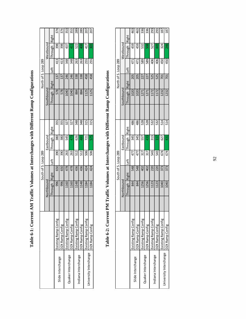
92

Ta

ble

6-1

: C

urr

ent

AM

Tra

ffic

Volu

mes

at

Inte

rch

an

ges

wit

h D

iffe

ren

t R

am

p C

on

fig

ura

tio

ns

Ta

ble

6-2

: C

urr

ent

PM

Tra

ffic

Volu

mes

at

Inte

rch

an

ges

wit

h D

iffe

ren

t R

am

p C

on

fig

ura

tio

ns

Thro

ugh

Rig

ht

Left

Thro

ugh

Rig

ht

Thro

ugh

Rig

ht

Left

Thro

ugh

Rig

ht

Exis

tin

g R

amp

Co

nfi

g99

665

039

038

035

557

813

741

339

837

4

D2X

Ram

p C

on

fig

996

650

390

380

355

578

137

413

398

374

Exis

tin

g R

amp

Co

nfi

g11

6047

826

354

532

710

4024

634

843

735

3

D2X

Ram

p C

on

fig

1160

478

263

473

327

1040

246

348

411

353

Exis

tin

g R

amp

Co

nfi

g11

4843

651

262

634

888

433

826

352

228

9

D2X

Ram

p C

on

fig

1148

436

512

480

348

884

338

263

408

289

Exis

tin

g R

amp

Co

nfi

g11

8442

450

672

131

511

2545

825

541

720

7

D2X

Ram

p C

on

fig

1184

424

506

575

315

1125

458

255

303

207

Slid

e In

terc

han

ge

Qu

ake

r In

terc

han

ge

Ind

ian

a In

terc

han

ge

Un

ive

rsit

y In

terc

han

ge

Sou

th o

f S.

Lo

op

289

No

rth

of

S. L

oo

p 2

89

No

rth

bo

un

dEa

stb

ou

nd

Sou

thb

ou

nd

We

stb

ou

nd

Thro

ugh

Rig

ht

Left

Thro

ugh

Rig

ht

Thro

ugh

Rig

ht

Left

Thro

ugh

Rig

ht

Exis

tin

g R

amp

Co

nfi

g84

454

847

734

548

610

2020

547

145

946

3

D2X

Ram

p C

on

fig

844

548

477

345

486

1020

205

471

459

463

Exis

tin

g R

amp

Co

nfi

g12

5640

231

755

752

812

7122

758

953

233

6

D2X

Ram

p C

on

fig

1256

402

317

433

528

1271

227

589

508

336

Exis

tin

g R

amp

Co

nfi

g11

2322

054

331

353

211

7252

540

652

729

3

D2X

Ram

p C

on

fig

1123

220

543

117

532

1172

525

406

449

293

Exis

tin

g R

amp

Co

nfi

g10

4037

367

462

751

412

3270

145

032

418

7

D2X

Ram

p C

on

fig

1040

373

674

431

514

1232

701

450

246

187

Slid

e In

terc

han

ge

Qu

ake

r In

terc

han

ge

Ind

ian

a In

terc

han

ge

Un

ive

rsit

y In

terc

han

ge

Sou

th o

f S.

Lo

op

289

No

rth

of

S. L

oo

p 2

89

No

rth

bo

un

dEa

stb

ou

nd

Sou

thb

ou

nd

We

stb

ou

nd

93

Ta

ble

6-3

: F

ore

cast

ed A

M T

raff

ic V

olu

mes

at

Inte

rch

an

ges

wit

h D

iffe

ren

t R

am

p C

on

fig

ura

tion

s

Ta

ble

6-4

: F

ore

cast

ed P

M T

raff

ic V

olu

mes

at

Inte

rch

an

ges

wit

h D

iffe

ren

t R

am

p C

on

fig

ura

tio

ns

Thro

ugh

Rig

ht

Left

Thro

ugh

Rig

ht

Thro

ugh

Rig

ht

Left

Thro

ugh

Rig

ht

Exis

tin

g R

amp

Co

nfi

g11

5575

445

244

141

267

015

947

946

143

4

D2X

Ram

p C

on

fig

1155

754

452

441

412

670

159

479

461

434

Exis

tin

g R

amp

Co

nfi

g13

4555

430

563

237

912

0628

540

350

740

9

D2X

Ram

p C

on

fig

1345

554

305

548

379

1206

285

403

476

409

Exis

tin

g R

amp

Co

nfi

g13

3150

559

472

640

310

2539

230

560

533

5

D2X

Ram

p C

on

fig

1331

505

594

556

403

1025

392

305

473

335

Exis

tin

g R

amp

Co

nfi

g13

7349

258

783

636

513

0453

129

648

324

0

D2X

Ram

p C

on

fig

1373

492

587

667

365

1304

531

296

351

240

Slid

e In

terc

han

ge

Qu

ake

r In

terc

han

ge

Ind

ian

a In

terc

han

ge

Un

ive

rsit

y In

terc

han

ge

Sou

th o

f S.

Lo

op

289

No

rth

of

S. L

oo

p 2

89

No

rth

bo

un

dEa

stb

ou

nd

Sou

thb

ou

nd

We

stb

ou

nd

Thro

ugh

Rig

ht

Left

Thro

ugh

Rig

ht

Thro

ugh

Rig

ht

Left

Thro

ugh

Rig

ht

Exis

tin

g R

amp

Co

nfi

g97

863

555

340

056

311

8223

854

653

253

7

D2X

Ram

p C

on

fig

978

635

553

400

563

1182

238

546

532

537

Exis

tin

g R

amp

Co

nfi

g14

5646

636

764

661

212

7122

768

361

739

0

D2X

Ram

p C

on

fig

1456

466

367

502

612

1271

227

683

589

390

Exis

tin

g R

amp

Co

nfi

g11

2322

062

936

361

711

7252

547

161

134

0

D2X

Ram

p C

on

fig

1123

220

629

136

617

1172

525

471

521

340

Exis

tin

g R

amp

Co

nfi

g10

4037

378

172

759

612

3270

152

237

621

7

D2X

Ram

p C

on

fig

1040

373

781

500

596

1232

701

522

285

217

Slid

e In

terc

han

ge

Qu

ake

r In

terc

han

ge

Ind

ian

a In

terc

han

ge

Un

ive

rsit

y In

terc

han

ge

Sou

th o

f S.

Lo

op

289

No

rth

of

S. L

oo

p 2

89

No

rth

bo

un

dEa

stb

ou

nd

Sou

thb

ou

nd

We

stb

ou

nd

94

6.2 Signal Timing Design

The research team used the signal timing phase order of the traditional TTI-4-Phase

Diamond interchange operation (as shown in Figure 6-1), which is used for operating most

Diamond interchanges in the City of Lubbock. The green time calculation method documented in

Chapter 10 and Chapter 16 of the HCM 2000 was applied for obtaining an equalizing saturation

degree of critical movements.

Figure 6-1: TTI-4-Phase Signal Timing Phase Design

An Excel program was developed for calculating green time with the inputs of traffic

volumes and lane configurations at interchanges. The calculated green time of each phase was

adjusted based on minimum green time and pedestrian traveling time to get practical signal

timing plans (shown in Table 6-1 and Table 6-2). The signal timing plans in Table 6-1 and Table

6-2 were designed based on current traffic volumes and existing geometric designs. The future

traffic was estimated by using a uniform traffic growth rate, 3%, in the study area, so traffic

volumes of each movement were increased by the same percentage. Therefore, the calculated

signal timing plans for future traffic were exactly the same as plans for current traffic. The only

impact of the alternatives to interchanges was a decrease of through movement traffic on

frontage roads, which was caused by the transformation from Diamond interchanges to X pattern

interchanges. During the process of signal timing design, only the critical movement V/C ratio

1 2 6 7

5 8 3 4

TTI-4 Phase Diamond Interchange Operation

95

impacts affected green time. For frontage road traffic, the left turn traffic movement is the

critical movement at each interchange of the study area. The transformation from Diamond

interchanges to X type interchanges, therefore, would not change the calculated signal timing

plans for existing Diamond interchanges. For this reason, signal timing plans for Diamond

interchanges and X type interchanges with current and forecasted traffic volumes will be the

same. During this research, the signal timing plans in Table 6-5 and Table 6-6 were employed for

the analysis of the improvement options.

6.3 Analysis Results

Using the estimated traffic volumes, interchange lane configurations, and designed signal

timing plans, Synchro models were built for the analysis of the three interchange operations

under the existing and forecasted traffic demands. Alternative 1 has one additional lane on the

freeway between each pair of on-ramps and off-ramps, so the traffic volumes at interchanges are

the same as the volumes for existing configurations. Alternative 2 and Alternative 3 both have X

type interchanges, which decrease through movement traffic volumes on frontage roads. The two

alternatives have the same estimated traffic volumes and designed signal timing plans at

interchanges. Thus, the team obtained the same analysis results for the existing design and

Alternative 1 and the same analysis results for Alternative 2 and Alternative 3.

The research team ran simulations with SimTraffic in order to accurately evaluate control

delay and LOS. The simulation results achieved are listed in Table 6-7 through Table 6-10.

The LOS values marked with green are the movements where LOS was improved after the

transformation from a Diamond interchange to an X type interchange. In fact, all control delays

of frontage road through movement at the Quaker Avenue interchange, Indiana Avenue

interchange, and University Avenue interchange were decreased by the Diamond to X pattern

change. However, only the improvements of the green-marked movements were enough to give

better LOS values.

By comparing the analysis results, it was found that Alternative 2 and Alternative 3

decreased control delays and provided better LOS for through movements on frontage roads. The

signal timing calculated by the equalizing V/C ratio method was not changed when Diamond

interchanges were transformed to X type interchanges, because the traffic volumes of the critical

movements would not be changed by the transformation. Therefore, the traffic of other

96

movements, including turning traffic on frontage roads and traffic on arterial roads, was not

benefitted by Alternative 2 and Alternative 3 under current traffic demand or future traffic

demand.

97

Tab

le 6

-5:

AM

Sig

nal

Tim

ing P

lan

Tab

le 6

-6:

PM

Sig

nal

Tim

ing P

lan

Cyc

le L

en

gth

Yell

ow

Tim

eA

ll-R

ed

Tim

eP

has

e 1

Ph

ase

2P

has

e 3

Ph

ase

4P

has

e 5

Ph

ase

6P

has

e 7

Ph

ase

8

Slid

e In

terc

han

ge13

04

223

4135

3156

588

8

Qu

ake

r In

terc

han

ge13

04

228

3430

3854

608

8

Ind

ian

a In

terc

han

ge13

04

226

3131

4249

658

8

Un

ive

rsit

y In

terc

han

ge13

04

229

2931

4150

648

8

Cyc

le L

en

gth

Yell

ow

Tim

eA

ll-R

ed

Tim

eP

has

e 1

Ph

ase

2P

has

e 3

Ph

ase

4P

has

e 5

Ph

ase

6P

has

e 7

Ph

ase

8

Slid

e In

terc

han

ge13

04

232

3528

3559

558

8

Qu

ake

r In

terc

han

ge13

04

229

3128

4252

628

8

Ind

ian

a In

terc

han

ge13

04

232

2631

4050

638

8

Un

ive

rsit

y In

terc

han

ge13

04

233

2929

3954

608

8

98

Ta

ble

6-7

: A

M L

OS

wit

h C

urr

ent

Tra

ffic

Volu

mes

at

Inte

rch

an

ges

wit

h D

iffe

ren

t R

am

p C

on

fig

ura

tio

ns

Ta

ble

6-8

: P

M L

OS

wit

h C

urr

ent

Tra

ffic

Volu

mes

at

Inte

rch

an

ges

wit

h D

iffe

ren

t R

am

p C

on

fig

ura

tio

ns

Thro

ugh

Rig

ht

Left

Thro

ugh

Rig

ht

Thro

ugh

Rig

ht

Left

Thro

ugh

Rig

ht

Exis

tin

g R

amp

Co

nfi

gC

DE

AD

DD

A

D2X

Ram

p C

on

fig

CD

EA

DD

DA

Exis

tin

g R

amp

Co

nfi

gD

DD

AD

DD

A

D2X

Ram

p C

on

fig

DD

DA

DD

DA

Exis

tin

g R

amp

Co

nfi

gD

DC

AE

DE

A

D2X

Ram

p C

on

fig

DD

CA

ED

DA

Exis

tin

g R

amp

Co

nfi

gD

CC

AD

EE

A

D2X

Ram

p C

on

fig

DC

CA

DE

DA

No

rth

of

S. L

oo

p 2

89

No

rth

bo

un

dEa

stb

ou

nd

Sou

thb

ou

nd

We

stb

ou

nd

Slid

e In

terc

han

ge

Qu

ake

r In

terc

han

ge

Ind

ian

a In

terc

han

ge

Un

ive

rsit

y In

terc

han

ge

Sou

th o

f S.

Lo

op

289

Thro

ugh

Rig

ht

Left

Thro

ugh

Rig

ht

Thro

ugh

Rig

ht

Left

Thro

ugh

Rig

ht

Exis

tin

g R

amp

Co

nfi

gD

DD

AD

DD

A

D2X

Ram

p C

on

fig

DD

DA

DD

DA

Exis

tin

g R

amp

Co

nfi

gD

DD

AD

ED

A

D2X

Ram

p C

on

fig

DD

DA

DD

DA

Exis

tin

g R

amp

Co

nfi

gD

DD

AE

EE

A

D2X

Ram

p C

on

fig

DD

DA

EE

DA

Exis

tin

g R

amp

Co

nfi

gD

DD

AE

EE

A

D2X

Ram

p C

on

fig

DD

DA

EE

DA

No

rth

of

S. L

oo

p 2

89

No

rth

bo

un

dEa

stb

ou

nd

Sou

thb

ou

nd

We

stb

ou

nd

Slid

e In

terc

han

ge

Qu

ake

r In

terc

han

ge

Ind

ian

a In

terc

han

ge

Un

ive

rsit

y In

terc

han

ge

Sou

th o

f S.

Lo

op

289

99

Ta

ble

6-9

: A

M L

OS

wit

h F

ore

cast

ed T

raff

ic V

olu

mes

at

Inte

rch

an

ges

wit

h D

iffe

ren

t R

am

p C

on

fig

ura

tio

ns

Ta

ble

6-1

0:

PM

LO

S w

ith

Fore

cast

ed T

raff

ic V

olu

mes

at

Inte

rch

an

ges

wit

h D

iffe

ren

t R

am

p C

on

fig

ura

tio

ns

Thro

ugh

Rig

ht

Left

Thro

ugh

Rig

ht

Thro

ugh

Rig

ht

Left

Thro

ugh

Rig

ht

Exis

tin

g R

amp

Co

nfi

gD

DE

AD

DD

A

D2X

Ram

p C

on

fig

DE

EA

DD

DA

Exis

tin

g R

amp

Co

nfi

gD

DD

AD

DD

A

D2X

Ram

p C

on

fig

DD

DA

DD

DA

Exis

tin

g R

amp

Co

nfi

gE

DD

AE

EE

A

D2X

Ram

p C

on

fig

ED

CA

EE

DA

Exis

tin

g R

amp

Co

nfi

gD

DC

AD

EE

A

D2X

Ram

p C

on

fig

DD

CA

DE

DA

No

rth

of

S. L

oo

p 2

89

No

rth

bo

un

dEa

stb

ou

nd

Sou

thb

ou

nd

We

stb

ou

nd

Slid

e In

terc

han

ge

Qu

ake

r In

terc

han

ge

Ind

ian

a In

terc

han

ge

Un

ive

rsit

y In

terc

han

ge

Sou

th o

f S.

Lo

op

289

Thro

ugh

Rig

ht

Left

Thro

ugh

Rig

ht

Thro

ugh

Rig

ht

Left

Thro

ugh

Rig

ht

Exis

tin

g R

amp

Co

nfi

gD

ED

AD

DD

A

D2X

Ram

p C

on

fig

DE

DA

DD

DA

Exis

tin

g R

amp

Co

nfi

gE

DD

AE

ED

A

D2X

Ram

p C

on

fig

ED

DA

ED

DA

Exis

tin

g R

amp

Co

nfi

gD

DD

AE

EE

A

D2X

Ram

p C

on

fig

DD

DA

EE

DA

Exis

tin

g R

amp

Co

nfi

gE

DD

AE

EE

A

D2X

Ram

p C

on

fig

ED

DA

EE

DA

No

rth

of

S. L

oo

p 2

89

No

rth

bo

un

dEa

stb

ou

nd

Sou

thb

ou

nd

We

stb

ou

nd

Slid

e In

terc

han

ge

Qu

ake

r In

terc

han

ge

Ind

ian

a In

terc

han

ge

Un

ive

rsit

y In

terc

han

ge

Sou

th o

f S.

Lo

op

289

99

7. WEAVING AND RAMP ANALYSIS

Weaving is defined as the crossing of two or more traffic streams traveling in the same

general direction along a significant length of highway without the aid of traffic control devices.

When an on-ramp is closely followed by an off-ramp and the two are joined by an auxiliary lane,

they form a weaving segment. If a one-lane on-ramp is closely followed by a one-lane off-ramp

and the two are not connected by an auxiliary lane, the merge and diverge movements are

considered separately using procedures for the analysis of ramp junctions (HCM2010). The

impacts of the proposed and existing ramps of South Loop 289 to the traffic along the main lanes

are caused by weaving, merging, and diverging movements at the junctions of the freeway and

ramps. Therefore, this study analyzed each junction by using a weaving or ramp junction

analysis procedure as necessary.

7.1 Rationale

Freeway weaving and ramp junction analysis is a very important aspect of this project.

Changing the ramps from Diamond to X pattern will cause a change of traffic on frontage roads,

freeway main lanes and ramps, especially around the junction areas of the main lanes and ramps.

The micro simulation analysis gives a very good understanding of the density and LOS values

for main lanes and frontage roads. The weaving and ramp analysis was specially studied for

traffic movement at the ramps. This process identifies any possible problem at junction areas and

helps the research group to provide a more effective recommendation.

7.2 Methodology

Chapter 24 and 25 of the HCM includes detailed information on how to determine to use

either weaving or ramp junction analysis. For the existing ramp configuration and Alternative 2,

ramps were directly connected to the outside lane of the main lanes, so the ramp analysis

procedure was applied for evaluating the LOS of the ramps. For Alternative 1 and Alternative 2,

an auxiliary lane was added to the freeway main lanes for connecting each pair of on ramp and

off ramp. Therefore, the weaving analysis procedure was used for evaluating the performance of

ramps and weaving segments.

For the weaving analysis, the essential data that were used were the main lane traffic

volumes and detailed on- and off-ramp volumes. Other data that were used were for the

100

determination of the lengths of the weaving segments and lengths of both acceleration and

deceleration lanes. Finally, existing volumes were used to determine the projected traffic

volumes for the next five years.

As presented in Tables 7-1 through 7-12, three ramp scenarios are detailed for both AM

and PM peak hour volumes and for both existing (2011) to future (2016) traffic volumes. The

four conditions are:

Existing Geometric Condition

Alternative 1: Weaving Analysis on Existing Condition

Alternative 2: Ramp Junction Analysis on X Pattern

Alternative 3: Weaving Analysis on X Pattern

First, the “Existing Geometric Condition” scenario represents the current geometric

design of South Loop 289 with an X pattern west of Quaker Avenue and Diamond Intersections

East of Quaker Avenue. Next, Alternative 1 uses the geometric conditions from the existing

condition, but assumes the addition of an auxiliary lane to connect the on/off ramp pairs.

Weaving analysis is used here. Next, Alternative 2 requires changing the existing geometric

design to the X Pattern system with no auxiliary lane to connect the on/off ramp pairs. Ramp

Junction Analysis is used here. Finally, Alternative 3 requires changing the existing geometric

design of the X Pattern system, with the addition of the auxiliary lane to connect the on/off ramp

pair.

7.3 Procedure

The method used to analyze the weaving segments and ramp junctions in this project was

the methodology specified in the HCM 2000, specifically chapters 24 and 25. From there,

Microsoft Excel was used to create spreadsheets to tabulate all the necessary information and

finally determine the LOS of each existing or proposed ramp.

Ramp Junction Analysis

The methodological process used to construct the ramp junction analysis is briefly

summarized below:

101

The data for through traffic on the Loop 289 main lanes and the on/off ramp traffic in

vehicles per hour were first determined to begin the analysis. Next, the proportion of

approaching freeway flow remaining in Lanes 1, 2, and 3 immediately upstream of the merge

point (PFM) is calculated using the through and ramp traffic volumes. Then the flow rate in Lanes

1 and 2 of the freeway immediately upstream of the merge point (V12) is calculated and

measured in passenger cars per hour. Next, the capacity of the downstream segment (VFO) is

calculated and measured in passenger cars per hour. Next, the length of the acceleration and

deceleration lanes, (LA) and (LD), respectively is calculated. These values were approximated

using Google Earth and measured in feet. Then the density of the segment (DR) is calculated.

Finally, from the density the LOS is computed using the criteria shown in Table 7-13. These

tables are detailed tables with density and LOS values as shown in Tables 7-1, 7-3, 7-5, and 7-7.

Weaving Analysis

The methodological process used to construct the weaving analysis is identical to the ramp

junction analysis; therefore, the detailed methodological process used to construct the

spreadsheets for the weaving analysis is detailed below.

All weaving segments are considered to be “Type A” in which weaving vehicles in both

directions must make one lane change to successfully complete a weaving maneuver

(HCM2010). First, the data for the thru traffic and ramp traffic on the Loop 289 main lanes and

the on/off ramp traffic in vehicles per hour is determined. Next, the total weaving flow rate in the

weaving segment (VM) is calculated, using the total ramp traffic volumes for the on/off ramp pair.

Then the total non-weaving flow rate in the weaving segment (VNW) is calculated. Next, the total

flow rate in the weaving segment (V) is calculated and measured in passenger cars per hour.

After this, the speed of weaving vehicles is determined by first assuming “unconstrained

operation;” if the conditions for unconstrained operation are not met, then the “constrained

operation” is assumed. For computation of the “unconstrained operation” first, the weaving

intensity factor for the prediction of the weaving speed (WW) and the weaving intensity factor for

the prediction of the non-weaving speed (WNW) are computed. Then both the weaving and non-

weaving speeds are computed as (SW) and (SNW), respectively.

102

Next, the number of lanes used by non-weaving vehicles (NW) is computed. If this value

is less than 1.4 “unconstrained operation” is assumed; if not, the same process is done again

using “constrained operation” parameters. Next, the saturation flow (S) is determined, followed

by the distance of the auxiliary lane (L). These values were approximated using Google Earth

and measured in feet. Then the density of the segment (DR) is calculated. Finally, from the

density the LOS is computed using the criteria shown in Table 7-13. These detailed tables show

density and LOS values as shown in Tables 7-2, 7-4, 7-6, and 7-8.

.

103

Table 7-1: Existing Geometric Conditions - 2011

WB Off 23.2 C

EB On 22.4 C

WB On 24.8 C

EB Off 23.6 C

WB Off 26.7 C

EB On 23.0 C

WB Off 28.6 D

EB On 27.5 D

WB On 27.6 D

EB Off 28.0 D

WB Off 23.4 C

EB On 26.2 C

WB On 23.7 C

EB Off 27.5 D

WB Off 22.6 C

EB On 23.5 C

WB On 19.5 C

EB Off 24.1 C

WB Off 23.9 C

EB On 21.0 C

WB On 25.0 C

EB Off 23.8 C

WB Off 26.0 C

EB On 21.9 C

WB Off 29.2 D

EB On 25.7 C

WB On 29.3 D

EB Off 29.3 D

WB Off 25.6 C

EB On 27.2 C

WB On 26.7 C

EB Off 29.8 D

WB Off 21.4 C

EB On 23.4 C

WB On 21.6 C

EB Off 24.6 C

AM PEAK

HOUR

VOLUME

West of Slide Rd.

East of Slide Rd.

West of Quaker Ave.

DR(pc/mi/ln) LOSAM/PM FREEWAY SEGMENT/LOCATION ON/OFF RAMP

East of Quaker Ave.

West of Indiana Ave.

East of Indiana Ave.

East of University Ave.

West of IH-27


West of IH-27

PM PEAK

HOUR

VOLUME

West of Slide Rd.

East of Slide Rd.

West of Quaker Ave.

East of Quaker Ave.



West of University Ave.


104

Table 7-2: Alternative 1 - Weaving Analysis on Existing Condition - 2011

East of Quaker Ave. WB Off

West of Indiana Ave. WB On

East of Indiana Ave. WB Off

West of University Ave. WB On

East of University Ave. WB Off

West of IH-27 WB On

East of Quaker Ave. EB On

West of Indiana Ave. EB Off

East of Indiana Ave. EB On

West of University Ave. EB Off

East of University Ave. EB On

West of IH-27 EB Off






West of IH-27 WB On







AM/PMWEAVING

SEGMENTFREEWAY SEGMENT/LOCATION ON/OFF RAMP

22.5 C

DR(pc/mi/ln) LOS

17.0 B

23.5 C

South of South

Loop 289

16.1 B

North of South

Loop 289

20.3 C

PM PEAK

HOUR

VOLUME

North of South

Loop 289

24.5 C

AM PEAK

HOUR

VOLUME

C21.9

C27.2

19.4 C

B

South of South

Loop 289

17.9

19.4 C

26.8 C

105

Table 7-3: Alternative 2 - Ramp Junction Analysis on X Pattern - 2011

WB Off 23.2 C

EB On 22.4 C

WB On 24.0 C

EB Off 18.8 B

WB Off 22.0 C

EB On 23.0 C

WB On 21.8 C

EB Off 27.7 D

WB Off 25.5 C

EB On 19.8 C

WB On 18.7 B

EB Off 29.5 D

WB Off 18.9 B

EB On 18.8 B

WB On 16.9 B

EB Off 25.9 C

WB Off 17.1 B

EB On 15.4 B

WB Off 23.8 C

EB On 21.0 C

WB On 25.0 C

EB Off 17.9 B

WB Off 19.3 C

EB On 21.9 C

WB On 20.0 C

EB Off 24.0 C

WB Off 30.1 D

EB On 23.4 C

WB On 17.8 B

EB Off 33.7 D

WB Off 21.7 C

EB On 21.1 C

WB On 15.4 B

EB Off 26.5 C

WB Off 16.5 B

EB On 19.5 C

AM PEAK

HOUR

VOLUME

West of Slide Rd.

East of Slide Rd.

West of Quaker Ave.

DR(pc/mi/ln) LOSAM/PM FREEWAY SEGMENT/LOCATION ON/OFF RAMP

East of Quaker Ave.




West of IH-27


West of IH-27

PM PEAK

HOUR

VOLUME

West of Slide Rd.

East of Slide Rd.

West of Quaker Ave.

East of Quaker Ave.





106

Table 7-4: Alternative 3 - Weaving Analysis on X Pattern - 2011

West of Slide Rd. WB Off

East of Slide Rd. WB On

West of Quaker Ave. WB Off

East of Quaker Ave. WB On

West of Indiana Ave. WB Off

East of Indiana Ave. WB On

West of University Ave. WB Off

East of University Ave. WB On

West of Slide Rd. EB On

East of Slide Rd. EB Off

West of Quaker Ave. EB On

East of Quaker Ave. EB Off

West of Indiana Ave. EB On

East of Indiana Ave. EB Off

West of University Ave. EB On

East of University Ave. EB Off

















AM/PMWEAVING


24.3 C

14.9 B

DR(pc/mi/ln) LOS

14.2 B

17.6 B

19.8 C

19.9 C

South of South

Loop 289

18.1 B

PM PEAK

HOUR

VOLUME

North of South

Loop 289

22.8 C

AM PEAK

HOUR

VOLUME

North of South

Loop 289

C26.6

B18.6

B

South of South

Loop 289

16.3

C23.3

C

16.6 B

21.2 C

17.9 B

26.8

107

Table 7-5: Existing Geometric Conditions - 2016

WB Off 29.7 D

EB On 25.6 C

WB On 28.4 D

EB Off 28.3 D

WB Off 32.4 D

EB On 25.8 C

WB Off 36.3 E

EB On 31.7 D

WB On 31.8 D

EB Off 34.9 D

WB Off 29.1 D

EB On 31.1 D

WB On 26.8 C

EB Off 33.8 D

WB Off 27.7 D

EB On 27.8 D

WB On 22.1 C

EB Off 29.7 D

WB Off 29.8 D

EB On 24.6 C

WB On 28.6 D

EB Off 28.1 D

WB Off 30.7 D

EB On 24.3 C

WB Off 36.3 E

EB On 29.4 D

WB On 34.0 D

EB Off 37.8 E

WB Off 31.7 D

EB On 33.8 D

WB On 29.8 D

EB Off 36.9 E

WB Off 26.1 C

EB On 28.5 D

WB On 24.1 C

EB Off 30.7 D

AM/PM FREEWAY SEGMENT/LOCATION ON/OFF RAMP

AM PEAK

HOUR

VOLUME

West of Slide Rd.

East of Slide Rd.


DR(pc/mi/ln) LOS

West of Quaker Ave.

East of Quaker Ave.

PM PEAK

HOUR

VOLUME

West of Slide Rd.

East of Slide Rd.

West of Quaker Ave.

East of Quaker Ave.





West of IH-27




West of IH-27

108

Table 7-6: Alternative 1 - Weaving Analysis on Existing Condition - 2016






West of IH-27 WB On












West of IH-27 WB On







AM/PMWEAVING


27.0 C

DR(pc/mi/ln) LOS

19.4 C

20.3 C

PM PEAK

HOUR

VOLUME

North of South

Loop 289

29.5 D

28.4 D

South of South

Loop 289

AM PEAK

HOUR

VOLUME

North of South

Loop 289

South of South

Loop 289

21.6

C26.5

32.3 D

23.3 C

C

D32.9

24.6 C

23.4 C

109

Table 7-7: Alternative 2 - Ramp Junction Analysis on X Pattern - 2016

WB Off 29.7 D

EB On 25.6 C

WB On 27.7 D

EB Off 22.0 C

WB Off 25.8 C

EB On 25.8 C

WB On 25.9 C

EB Off 31.8 D

WB Off 29.9 D

EB On 23.3 C

WB On 21.9 C

EB Off 34.0 D

WB Off 22.4 C

EB On 22.2 C

WB On 19.6 C

EB Off 29.9 D

WB Off 19.8 C

EB On 17.6 B

WB Off 29.7 D

EB On 24.6 C

WB On 28.6 D

EB Off 20.5 C

WB Off 22.1 C

EB On 24.3 C

WB On 23.4 C

EB Off 27.9 D

WB Off 34.6 D

EB On 28.3 D

WB On 20.3 C

EB Off 39.3 E

WB Off 25.1 C

EB On 25.7 C

WB On 17.6 B

EB Off 31.2 D

WB Off 19.3 B

EB On 23.6 C




West of IH-27




West of IH-27

PM PEAK

HOUR

VOLUME

West of Slide Rd.

East of Slide Rd.

West of Quaker Ave.

East of Quaker Ave.


West of Quaker Ave.

East of Quaker Ave.


DR(pc/mi/ln) LOS

AM PEAK

HOUR

VOLUME

West of Slide Rd.

East of Slide Rd.

AM/PM FREEWAY SEGMENT/LOCATION ON/OFF RAMP

110

Table 7-8: Alternative 3 - Weaving Analysis on X Pattern – 2016

































AM/PMWEAVING


29.4 D

17.7 B

DR(pc/mi/ln) LOS

17.0 B

21.2 C

23.8 C

24.0 C

South of South

Loop 289

21.8 C

PM PEAK

HOUR

VOLUME

North of South

Loop 289

27.6 D

AM PEAK

HOUR

VOLUME

North of South

Loop 289

South of South

Loop 289

19.6

D28.3

32.5 D

19.9 C

25.6 C

C

D32.3

C22.3

21.4 C

111

7.4

Stu

dy R

esu

lts

Tab

le 7

-9:

An

aly

sis

Su

mm

ary

– 2

011/A

M P

eak

RA

MP

DES

CR

IPTI

ON

ON

/OFF

RA

MP

WB

ON

EB O

FFW

B O

FFEB

ON

WB

OFF

EB O

NW

B O

NEB

OFF

WB

OFF

EB O

NW

B O

NEB

OFF

WB

OFF

EB O

NW

B O

NEB

OFF

LEV

EL O

F SE

RV

ICE

(LO

S)C

CC

CD

DD

DC

CC

DC

CC

C

RA

MP

DES

CR

IPTI

ON

ON

/OFF

RA

MP

WB

ON

EB O

FFW

B O

FFEB

ON

WB

OFF

EB O

NW

B O

NEB

OFF

WB

OFF

EB O

NW

B O

NEB

OFF

WB

OFF

EB O

NW

B O

NEB

OFF

LEV

EL O

F SE

RV

ICE

(LO

S)C

CC

CC

CC

CB

CB

CB

CB

C

RA

MP

DES

CR

IPTI

ON

ON

/OFF

RA

MP

WB

ON

EB O

FFW

B O

FFEB

ON

WB

OFF

EB O

NW

B O

NEB

OFF

WB

OFF

EB O

NW

B O

NEB

OFF

WB

OFF

EB O

NW

B O

NEB

OFF

LEV

EL O

F SE

RV

ICE

(LO

S)C

BC

CC

CC

DB

BB

DB

BB

C

RA

MP

DES

CR

IPTI

ON

ON

/OFF

RA

MP

WB

ON

EB O

FFW

B O

FFEB

ON

WB

OFF

EB O

NW

B O

NEB

OFF

WB

OFF

EB O

NW

B O

NEB

OFF

WB

OFF

EB O

NW

B O

NEB

OFF

LEV

EL O

F SE

RV

ICE

(LO

S)B

CC

CB

CC

CB

BB

CB

B

DEN

SITY

IN T

HE

MER

GIN

G

INFL

UEN

CE

AR

EA (

pc/

mi/

ln)

22

.52

0.3

29

.52

5.5

19

.82

1.8

20

.31

6.1

20

.32

2.5

20

.32

4.5

17

.02

4.5

16

.1

YEA

R 2

01

1 -

AM

PEA

K -

ALT

ERN

ATI

VE

1 -

WEA

VIN

G A

NA

LYSI

S O

N E

XIS

TIN

G C

ON

DIT

ION

YEA

R 2

01

1 -

AM

PEA

K -

ALT

ERN

ATI

VE

3 -

WEA

VIN

G A

NA

LYSI

S O

N X

PA

TTER

N

14

.21

8.1

17

.11

5.4

16

.92

5.9

BET

WEE

N S

LID

E A

ND

QU

AK

ERB

ETW

EEN

QU

AK

ER A

ND

IND

IAN

AB

ETW

EEN

IND

IAN

A A

ND

UN

IVER

SITY

BET

WEE

N U

NIV

ERSI

TY A

ND

IH-2

7

BET

WEE

N S

LID

E A

ND

QU

AK

ERB

ETW

EEN

QU

AK

ER A

ND

IND

IAN

AB

ETW

EEN

IND

IAN

A A

ND

UN

IVER

SITY

BET

WEE

N U

NIV

ERSI

TY A

ND

IH-2

7

22

.52

3.5

17

.02

2.5

23

.5

YEA

R 2

01

1 -

AM

PEA

K -

ALT

ERN

ATI

VE

2 -

RA

MP

JU

NC

TIO

N A

NA

LYSI

S O

N X

PA

TTER

N

YEA

R 2

01

1 -

AM

PEA

K -

EX

ISTI

NG

GEO

MET

RIC

CO

ND

TIO

N

19

.52

4.1

22

.62

3.5

28

.62

7.5

27

.62

8.0

23

.42

6.2

23

.72

7.5

26

.72

3.0

DEN

SITY

IN T

HE

MER

GIN

G

INFL

UEN

CE

AR

EA (

pc/

mi/

ln)

24

.82

3.6

BET

WEE

N S

LID

E A

ND

QU

AK

ERB

ETW

EEN

QU

AK

ER A

ND

IND

IAN

AB

ETW

EEN

IND

IAN

A A

ND

UN

IVER

SITY

BET

WEE

N U

NIV

ERSI

TY A

ND

IH-2

7

DEN

SITY

IN T

HE

MER

GIN

G

INFL

UEN

CE

AR

EA (

pc/

mi/

ln)

24

.01

8.8

22

.02

3.0

BET

WEE

N S

LID

E A

ND

QU

AK

ERB

ETW

EEN

QU

AK

ER A

ND

IND

IAN

A

18

.81

8.7

27

.71

8.9

22

.81

7.6

22

.82

4.3

19

.81

4.2

BET

WEE

N IN

DIA

NA

AN

D U

NIV

ERSI

TY

DEN

SITY

IN T

HE

MER

GIN

G

INFL

UEN

CE

AR

EA (

pc/

mi/

ln)

14

.91

9.9

24

.31

9.8

18

.11

7.6

BET

WEE

N U

NIV

ERSI

TY A

ND

IH-2

7

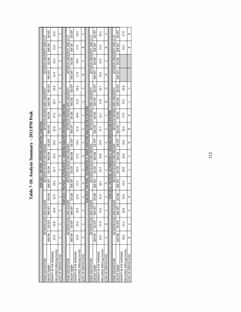
112

Tab

le 7

-10:

An

aly

sis

Su

mm

ary

– 2

011/P

M P

eak

RA

MP

DES

CR

IPTI

ON

ON

/OFF

RA

MP

WB

ON

EB O

FFW

B O

FFEB

ON

WB

OFF

EB O

NW

B O

NEB

OFF

WB

OFF

EB O

NW

B O

NEB

OFF

WB

OFF

EB O

NW

B O

NEB

OFF

LEV

EL O

F SE

RV

ICE

(LO

S)C

CC

CD

CD

DC

DC

DC

CC

C

RA

MP

DES

CR

IPTI

ON

ON

/OFF

RA

MP

WB

ON

EB O

FFW

B O

FFEB

ON

WB

OFF

EB O

NW

B O

NEB

OFF

WB

OFF

EB O

NW

B O

NEB

OFF

WB

OFF

EB O

NW

B O

NEB

OFF

LEV

EL O

F SE

RV

ICE

(LO

S)C

CC

CD

CD

CC

CC

CB

CB

C

RA

MP

DES

CR

IPTI

ON

ON

/OFF

RA

MP

WB

ON

EB O

FFW

B O

FFEB

ON

WB

OFF

EB O

NW

B O

NEB

OFF

WB

OFF

EB O

NW

B O

NEB

OFF

WB

OFF

EB O

NW

B O

NEB

OFF

LEV

EL O

F SE

RV

ICE

(LO

S)C

BC

CD

CC

CC

CB

DB

CB

C

RA

MP

DES

CR

IPTI

ON

ON

/OFF

RA

MP

WB

ON

EB O

FFW

B O

FFEB

ON

WB

OFF

EB O

NW

B O

NEB

OFF

WB

OFF

EB O

NW

B O

NEB

OFF

WB

OFF

EB O

NW

B O

NEB

OFF

LEV

EL O

F SE

RV

ICE

(LO

S)B

CC

BC

CC

BB

BC

CB

B

YEA

R 2

01

1 -

PM

PEA

K -

EX

ISTI

NG

GEO

MET

RIC

CO

ND

TIO

N

BET

WEE

N S

LID

E A

ND

QU

AK

ERB

ETW

EEN

QU

AK

ER A

ND

IND

IAN

AB

ETW

EEN

IND

IAN

A A

ND

UN

IVER

SITY

BET

WEE

N U

NIV

ERSI

TY A

ND

IH-2

7

YEA

R 2

01

1 -

PM

PEA

K -

ALT

ERN

ATI

VE

1 -

WEA

VIN

G A

NA

LYSI

S O

N E

XIS

TIN

G C

ON

DIT

ION

BET

WEE

N S

LID

E A

ND

QU

AK

ERB

ETW

EEN

QU

AK

ER A

ND

IND

IAN

AB

ETW

EEN

IND

IAN

A A

ND

UN

IVER

SITY

BET

WEE

N U

NIV

ERSI

TY A

ND

IH-2

7

27

.22

6.7

29

.82

1.4

23

.42

9.2

25

.72

9.3

29

.32

5.6

DEN

SITY

IN T

HE

MER

GIN

G

INFL

UEN

CE

AR

EA (

pc/

mi/

ln)

25

.02

3.8

26

.02

1.9

21

.62

4.6

17

.91

9.4

YEA

R 2

01

1 -

PM

PEA

K -

ALT

ERN

ATI

VE

2 -

RA

MP

JU

NC

TIO

N A

NA

LYSI

S O

N X

PA

TTER

N

BET

WEE

N S

LID

E A

ND

QU

AK

ERB

ETW

EEN

QU

AK

ER A

ND

IND

IAN

AB

ETW

EEN

IND

IAN

A A

ND

UN

IVER

SITY

BET

WEE

N U

NIV

ERSI

TY A

ND

IH-2

7

26

.82

1.9

26

.81

7.9

19

.42

7.2

19

.42

7.2

19

.42

1.9

DEN

SITY

IN T

HE

MER

GIN

G

INFL

UEN

CE

AR

EA (

pc/

mi/

ln)

25

.92

1.6

25

.92

1.6

15

.42

6.5

YEA

R 2

01

1 -

PM

PEA

K -

ALT

ERN

ATI

VE

3 -

WEA

VIN

G A

NA

LYSI

S O

N X

PA

TTER

N

BET

WEE

N S

LID

E A

ND

QU

AK

ERB

ETW

EEN

QU

AK

ER A

ND

IND

IAN

AB

ETW

EEN

IND

IAN

A A

ND

UN

IVER

SITY

BET

WEE

N U

NIV

ERSI

TY A

ND

IH-2

7

21

.11

7.8

33

.71

6.5

19

.53

0.1

23

.42

0.0

24

.02

1.7

DEN

SITY

IN T

HE

MER

GIN

G

INFL

UEN

CE

AR

EA (

pc/

mi/

ln)

25

.01

7.9

19

.32

1.9

16

.31

7.9

17

.92

3.3

26

.82

3.3

26

.82

6.6

16

.61

6.3

DEN

SITY

IN T

HE

MER

GIN

G

INFL

UEN

CE

AR

EA (

pc/

mi/

ln)

18

.62

1.2

26

.61

6.6

113

Tab

le 7

-11

: A

naly

sis

Su

mm

ary

– 2

016/A

M P

eak

RA

MP

DES

CR

IPTI

ON

ON

/OFF

RA

MP

WB

ON

EB O

FFW

B O

FFEB

ON

WB

OFF

EB O

NW

B O

NEB

OFF

WB

OFF

EB O

NW

B O

NEB

OFF

WB

OFF

EB O

NW

B O

NEB

OFF

LEV

EL O

F SE

RV

ICE

(LO

S)D

DD

CE

DD

DD

DC

DD

DC

D

RA

MP

DES

CR

IPTI

ON

ON

/OFF

RA

MP

WB

ON

EB O

FFW

B O

FFEB

ON

WB

OFF

EB O

NW

B O

NEB

OFF

WB

OFF

EB O

NW

B O

NEB

OFF

WB

OFF

EB O

NW

B O

NEB

OFF

LEV

EL O

F SE

RV

ICE

(LO

S)C

CC

CC

DC

DC

DC

DC

CC

C

RA

MP

DES

CR

IPTI

ON

ON

/OFF

RA

MP

WB

ON

EB O

FFW

B O

FFEB

ON

WB

OFF

EB O

NW

B O

NEB

OFF

WB

OFF

EB O

NW

B O

NEB

OFF

WB

OFF

EB O

NW

B O

NEB

OFF

LEV

EL O

F SE

RV

ICE

(LO

S)D

CC

CD

CC

DC

CC

DC

BC

D

RA

MP

DES

CR

IPTI

ON

ON

/OFF

RA

MP

WB

ON

EB O

FFW

B O

FFEB

ON

WB

OFF

EB O

NW

B O

NEB

OFF

WB

OFF

EB O

NW

B O

NEB

OFF

WB

OFF

EB O

NW

B O

NEB

OFF

LEV

EL O

F SE

RV

ICE

(LO

S)B

CD

CC

DD

CB

CC

DB

C

YEA

R 2

01

6 -

AM

PEA

K -

EX

ISTI

NG

GEO

MET

RIC

CO

ND

TIO

N

BET

WEE

N S

LID

E A

ND

QU

AK

ERB

ETW

EEN

QU

AK

ER A

ND

IND

IAN

AB

ETW

EEN

IND

IAN

A A

ND

UN

IVER

SITY

BET

WEE

N U

NIV

ERSI

TY A

ND

IH-2

7

22

.12

9.7

YEA

R 2

01

6 -

AM

PEA

K -

ALT

ERN

ATI

VE

1 -

WEA

VIN

G A

NA

LYSI

S O

N E

XIS

TIN

G C

ON

DIT

ION

BET

WEE

N S

LID

E A

ND

QU

AK

ERB

ETW

EEN

QU

AK

ER A

ND

IND

IAN

AB

ETW

EEN

IND

IAN

A A

ND

UN

IVER

SITY

BET

WEE

N U

NIV

ERSI

TY A

ND

IH-2

7

31

.12

6.8

33

.82

7.7

27

.83

6.3

31

.73

1.8

34

.92

9.1

DEN

SITY

IN T

HE

MER

GIN

G

INFL

UEN

CE

AR

EA (

pc/

mi/

ln)

28

.42

8.3

32

.42

5.8

19

.42

4.6

YEA

R 2

01

6 -

AM

PEA

K -

ALT

ERN

ATI

VE

2 -

RA

MP

JU

NC

TIO

N A

NA

LYSI

S O

N X

PA

TTER

N

BET

WEE

N S

LID

E A

ND

QU

AK

ERB

ETW

EEN

QU

AK

ER A

ND

IND

IAN

AB

ETW

EEN

IND

IAN

A A

ND

UN

IVER

SITY

BET

WEE

N U

NIV

ERSI

TY A

ND

IH-2

7

29

.52

0.3

29

.51

9.4

24

.62

7.0

28

.42

7.0

28

.42

0.3

DEN

SITY

IN T

HE

MER

GIN

G

INFL

UEN

CE

AR

EA (

pc/

mi/

ln)

25

.92

4.5

25

.92

4.5

19

.62

9.9

YEA

R 2

01

6 -

AM

PEA

K -

ALT

ERN

ATI

VE

3 -

WEA

VIN

G A

NA

LYSI

S O

N X

PA

TTER

N

BET

WEE

N S

LID

E A

ND

QU

AK

ERB

ETW

EEN

QU

AK

ER A

ND

IND

IAN

AB

ETW

EEN

IND

IAN

A A

ND

UN

IVER

SITY

BET

WEE

N U

NIV

ERSI

TY A

ND

IH-2

7

22

.22

1.9

34

.01

9.8

17

.62

9.9

23

.32

5.9

31

.82

2.4

DEN

SITY

IN T

HE

MER

GIN

G

INFL

UEN

CE

AR

EA (

pc/

mi/

ln)

27

.72

2.0

25

.82

5.8

17

.02

1.8

21

.82

1.2

27

.62

1.2

27

.62

9.4

23

.81

7.0

DEN

SITY

IN T

HE

MER

GIN

G

INFL

UEN

CE

AR

EA (

pc/

mi/

ln)

17

.72

4.0

29

.42

3.8

114

Tab

le 7

-12:

An

aly

sis

Su

mm

ary

– 2

016/P

M P

eak

Tab

le 7

-13

: L

OS

Cri

teri

a f

or

Ram

p J

un

ctio

ns

RA

MP

DES

CR

IPTI

ON

ON

/OFF

RA

MP

WB

ON

EB O

FFW

B O

FFEB

ON

WB

OFF

EB O

NW

B O

NEB

OFF

WB

OFF

EB O

NW

B O

NEB

OFF

WB

OFF

EB O

NW

B O

NEB

OFF

LEV

EL O

F SE

RV

ICE

(LO

S)D

DD

CE

DD

ED

DD

EC

DC

D

RA

MP

DES

CR

IPTI

ON

ON

/OFF

RA

MP

WB

ON

EB O

FFW

B O

FFEB

ON

WB

OFF

EB O

NW

B O

NEB

OFF

WB

OFF

EB O

NW

B O

NEB

OFF

WB

OFF

EB O

NW

B O

NEB

OFF

LEV

EL O

F SE

RV

ICE

(LO

S)D

CD

CD

CD

CC

DC

DC

CC

C

RA

MP

DES

CR

IPTI

ON

ON

/OFF

RA

MP

WB

ON

EB O

FFW

B O

FFEB

ON

WB

OFF

EB O

NW

B O

NEB

OFF

WB

OFF

EB O

NW

B O

NEB

OFF

WB

OFF

EB O

NW

B O

NEB

OFF

LEV

EL O

F SE

RV

ICE

(LO

S)D

CC

CD

DC

DC

CC

EC

CB

D

RA

MP

DES

CR

IPTI

ON

ON

/OFF

RA

MP

WB

ON

EB O

FFW

B O

FFEB

ON

WB

OFF

EB O

NW

B O

NEB

OFF

WB

OFF

EB O

NW

B O

NEB

OFF

WB

OFF

EB O

NW

B O

NEB

OFF

LEV

EL O

F SE

RV

ICE

(LO

S)C

CD

CD

DD

CC

CD

DC

C

YEA

R 2

01

6 -

PM

PEA

K -

EX

ISTI

NG

GEO

MET

RIC

CO

ND

TIO

N

BET

WEE

N S

LID

E A

ND

QU

AK

ERB

ETW

EEN

QU

AK

ER A

ND

IND

IAN

AB

ETW

EEN

IND

IAN

A A

ND

UN

IVER

SITY

BET

WEE

N U

NIV

ERSI

TY A

ND

IH-2

7

26

.1

24

.13

0.7

YEA

R 2

01

6 -

PM

PEA

K -

ALT

ERN

ATI

VE

1 -

WEA

VIN

G A

NA

LYSI

S O

N E

XIS

TIN

G C

ON

DIT

ION

BET

WEE

N S

LID

E A

ND

QU

AK

ERB

ETW

EEN

QU

AK

ER A

ND

IND

IAN

AB

ETW

EEN

IND

IAN

A A

ND

UN

IVER

SITY

BET

WEE

N U

NIV

ERSI

TY A

ND

IH-2

7

33

.82

9.8

36

.92

6.1

28

.53

6.3

29

.43

4.0

37

.83

1.7

DEN

SITY

IN T

HE

MER

GIN

G

INFL

UEN

CE

AR

EA (

pc/

mi/

ln)

28

.62

8.1

30

.72

4.3

20

.52

2.1

24

.3

21

.62

3.4

YEA

R 2

01

6 -

PM

PEA

K -

ALT

ERN

ATI

VE

2 -

RA

MP

JU

NC

TIO

N A

NA

LYSI

S O

N X

PA

TTER

N

BET

WEE

N S

LID

E A

ND

QU

AK

ERB

ETW

EEN

QU

AK

ER A

ND

IND

IAN

AB

ETW

EEN

IND

IAN

A A

ND

UN

IVER

SITY

BET

WEE

N U

NIV

ERSI

TY A

ND

IH-2

7

32

.32

6.5

32

.32

1.6

23

.43

2.9

23

.33

2.9

23

.32

6.5

DEN

SITY

IN T

HE

MER

GIN

G

INFL

UEN

CE

AR

EA (

pc/

mi/

ln)

31

.42

6.1

31

.4

DEN

SITY

IN T

HE

MER

GIN

G

INFL

UEN

CE

AR

EA (

pc/

mi/

ln)

22

.32

5.6

32

.31

9.9

17

.63

1.2

YEA

R 2

01

6 -

PM

PEA

K -

ALT

ERN

ATI

VE

3 -

WEA

VIN

G A

NA

LYSI

S O

N X

PA

TTER

N

BET

WEE

N S

LID

E A

ND

QU

AK

ERB

ETW

EEN

QU

AK

ER A

ND

IND

IAN

AB

ETW

EEN

IND

IAN

A A

ND

UN

IVER

SITY

BET

WEE

N U

NIV

ERSI

TY A

ND

IH-2

7

25

.72

0.3

39

.31

9.3

23

.63

4.9

28

.32

3.4

27

.92

5.1

DEN

SITY

IN T

HE

MER

GIN

G

INFL

UEN

CE

AR

EA (

pc/

mi/

ln)

28

.6

19

.62

1.4

21

.42

8.3

32

.52

8.3

32

.53

2.3

19

.91

9.6

A B C D E

> 19

-27

> 27

-35

> 35

LOS

Mai

nla

ne

De

snit

y

pc/

mi/

ln

<= 1

0

> 10

-19

115

The summary analyses of Tables 7-9 through 7-12 show several distinct patterns which

are important to the analysis. When “Existing Geometric Condition,” as the control, is compared

to Alternatives 1-3, the densities and LOS values decrease the most with the implementation of

Alternative 3. On the contrary, Alternative 1 and 2 have a more consistent variance, with

Alternative 2 decreasing the density in several key intersections, such as between Quaker and

Indiana, but the benefits appear to be less profound. All alternatives have better densities than the

existing condition. Finally, these patterns reoccur through the AM and PM hours and the 2016

projections.

7.5 Conclusion

The weaving and ramp junction analyses presented in Tables 7-1 through 7-8 illustrate that

the proposed re-design of the existing Diamond ramps to X pattern ramps have a significant

impact on the mainlane traffic at ramp junctions. Furthermore, the analysis shows that X pattern

ramps without the addition of the auxiliary lane will also help reduce congestion to a modest

amount. Finally, the analysis shows that the use of Alternative 1, which results in the addition of

only an auxiliary lane, will also have a moderate impact on the traffic density. Alternative 1 is a

great option for a quick fix; however, Alternative 3, being the most costly option, would

significantly alleviate the problem for many years to come.

116

8. CONCLUSIONS

Three capacity improvement strategies, namely Alternative 1 (A1), Alternative 2 (A2), and

Alternative 3 (A3) were evaluated in this project, particularly focusing on the potential impact on

the frontage roads and intersections along South Loop 289. Alternative 1 involves adding an

auxiliary lane to the outside main lane between each entrance and exit ramps on both the

eastbound and westbound directions of South Loop 289 at Slide Road and Quaker Avenue,

Quaker Avenue and Indiana Avenue, Indiana Avenue and University Avenue, and University

Avenue and IH-27. Alternative 2 changes the ramp configuration from a Diamond to an X

pattern at Quaker Avenue, Indiana Avenue, and University Avenue. Considering that providing

an X pattern interchange will increase traffic volume on the frontage road, an auxiliary lane is

added to the frontage road between each exit and entrance ramp. Alternative 3 is developed on

the basis of Alternative 2, but provides the auxiliary lanes over the bridges on both eastbound

and westbound directions.

Traffic simulation models were developed in both VISSIM and Synchro to examine the

effectiveness of the three alternative strategies with regard to both current and forecasted traffic

demands.

Alternative 1 improves the level of service through added capacity on the main lanes of the

corridor. This will not affect the traffic distribution between the main lane and the frontage roads,

thus the LOS on the frontage road remains unchanged.

Alternative 2 alleviates the level of traffic density significantly on the main lanes by

converting the ramp configuration from a Diamond to an X pattern. The auxiliary lane is

necessary on the frontage to accommodate the increased traffic volumes diverted from the main

lanes. However, Alternative 2 will significantly increase the traffic volume on the frontage roads.

However, an auxiliary lane on the frontage road can effectively accomodate the increased traffic

volume and the perfomance of the frontage roads will remain at the same level as the current

network configuration.

Alternative 3 further supplements Alternative 2 by adding an auxiliary lane on the bridges.

The resulting performance is almost the same as that of Alternative 2 for both frontage and main

lane traffic segments.

117

For the analysis on the performance of intersections, it was revealed that Alternative 2 and

Alternative 3 decreased control delays and provided better LOS for through movements on

frontage roads. The signal timing calculated by the equalizing V/S ratio method was not changed

when Diamond interchanges were transformed to X type interchanges, because the traffic

volumes of the critical movements would not be changed by the transformation. Therefore, the

traffic of other movements, including turning traffic on frontage roads and traffic on arterial

roads was not benefited by Alternative 2 or Alternative 3 under current traffic demand and future

traffic demand.

It was additionally found through weaving analysis that all three alternatives would lead to

reduced weaving congestion. Even Alternative 1 would have a significant impact on the weaving

congestion. Alternative 3 would have the most significant impact, but it is only recommended if

a large amount of funding is available.

The findings from this research project lead to the following recommends:

With limited construction funding, the research team suggests Alternative 1 to alleviate

traffic congestion along the main lanes of South Loop 289. LOS, traffic merging, and safety

around joint points of on-ramps and main lanes will all be improved without impact to frontage

roads and intersections.

With enough construction funding, the research team suggests Alternative 3, which

provides better LOS on main lanes, longer weaving distances for weaving traffic and better

traffic safety at the joint points of on-ramps and main lanes. Traffic volumes on frontage roads

will be increased, but their LOS will be close to the existing situation because of the added

auxiliary lane. The control delay of through movements on frontage roads at interchanges will be

decreased. However, the whole interchange operation will not get much benefit from the

interchange transformation from Diamond to X. Alternative 3 is the best improvement option.

Alternative 2 can improve the LOS of the freeway main lanes and alleviate congestion on

the freeways, especially on the outside lanes. The impact to frontage roads and interchanges will

be the same as with Alternative 3. Without an auxiliary lane for weaving traffic, temporary

congestion may still happen at the joint points of on-ramps and main lanes because of limited

space for traffic merging action.

118

9. REFERENCES

1. AASHTO. A Policy on Geometric Design of Highways and Streets. American Association

of State Highway and Transportation Officials, Washington, D.C., 2004.

2. Dorothy, P. W., R. Ambadipudi, and R. M. Kill. Development and Validation of Large-

Scale Microscopic Models. Presented at 85th Annual Meeting of the Transportation

Research Board, Washington, D.C., 2006.

3. Chitturi, M. V., and R. F. Benekohal. Calibration of VISSIM for Freeways. Presented at

85th Annual Meeting of the Transportation Research Board, Washington, D.C., 2008.

4. Bloomberg, L., and J. Dale. A Comparison of the VISSIM and CORSIM Traffic Simulation

Models on a Congested Network. Presented at 79th Annual Meeting of the Transportation

Research Board, Washington, D.C., 2000.

5. Fellendorf M. VISSIM: A microscopic Simulation Tool to Evaluate Actuated Signal Control

including Bus Priority. Presented at the 64th

ITE Annual Meeting. 1994.

6. Frawley, W. E., and W. L. Eisele. Access management Guidebook for Texas. Publication

FHWA/TX-05/0-4141-P3. Texas Transportation Institute, 2005.

7. Flynn, M., W. Feuer, E. Janoff, M. Newman, A. Wiley-Schwartz. A 21st – Century Vision

of Street: Developing Street Design Guidelines as a Tool for Comprehensive Design.

Presented at 89th Annual Meeting of the Transportation Research Board, Washington, D.C.,

2010.

8. Fellendorf, M., and P. Vortisch. Validation of the Microscopic Traffic Flow Model

9. VISSIM in Different Real-World Situations. PTV America, 2005.

10. E. G. Velez. Adaptation of Vissim, A Dynamic Simulation Model, to the Traffic Behavior at

Intersections in Mayaguez, Puerto Rico. University of Puerto Rico, Mayaguez, 2006.

11. Pecheux, K. K., K. E. Barns K, and R. H. Henk. U.S. 83 Mail Lane, Ramp, and Cross-Street

Interchange Operational Analysis: McAllen, Texas. Publication TX-96/2903-4F. Texas

Transportation Institute, 1995.

12. Nelson, A. A., J. M. Tydlacka, R. G. Stevens, S. T. Chrysler, and A. P. Voigt. Lane

Assignment Traffic Control Devices on Frontage Roads and Conventional Roads at

119

Interchanges: Technical Report. Publication FHWA/TX-11/0-6106-1, Texas Transportation

Institute, 2010.

13. ODOT. Network or Corridor Simulation Models, Chapter 8, Analysis Procedures Manual.

Oregon Department of Transportation, Salem, OR, 2007.

14. PTV. VISSIM 4.10 User Manual. PTV AG, Karlsruhe, Germany, 2005.

15. PTV. VISSIM- State-of-the-Art Multi-Modal Simulation. PTV AG, Karlsruhe, Germany,

2005.

16. Cooner, S. A., S. Venglar, Y. Rathod, E. J. Pultorak, J. C. Williams, P. Vo, and S. P.

Mattingly. Ramp Reversal Project: Guidelines for Successful Implementation. Publication

FHWA/TX-07/0-5105-1, Texas Transportation Institute, 2007.

17. Trafficware. Synchro Studio 7 User Guide. Trafficware, Sugar Land, TX, 2006.

loop 289 corridor study - phase ii - texas tech · loop 289 corridor study - phase ii . loop 289...

Documents