look-ahead decision making for renewable energy: a dynamic
TRANSCRIPT
Applied Energy 296 (2021) 117068
A0
Contents lists available at ScienceDirect
Applied Energy
journal homepage: www.elsevier.com/locate/apenergy
Look-ahead decision making for renewable energy: A dynamic ‘‘predict andstore’’ approach✩
Jingxing Wang, Seokhyun Chung, Abdullah AlShelahi, Raed Kontar ∗, Eunshin Byon,Romesh SaigalDepartment of Industrial & Operations Engineering, University of Michigan, Ann Arbor, MI 48109, USA
A R T I C L E I N F O
Keywords:Renewable energyBattery storageLook-ahead optimizationJoint prediction and prescriptionFunctional principal component analysisBayesian inference
A B S T R A C T
This paper presents an integrative methodology for managing and stabilizing the output of a wind/solar farmusing storage devices in a cost effective and real-time manner. We consider the problem where a renewablefarm should decide the amount of energy charged into, or withdrawn from, the battery given the stochastic andtime-varying nature in the renewable energy power output. Our methodology features a seamless integrationof a non-myopic decision framework and a sequential non-parametric predictive model based on functionalprincipal component analysis. A key feature of our algorithm is that it quantifies costs over a rolling horizonwhere both predictions and decisions are updated on the fly as new data is acquired. Our technology is testedon the California ISO dataset. The case study provides a proof-of-concept that highlights both the benefits andease of implementation of our forward looking framework.
1. Introduction
Recently there has been considerable emphasis on replacing thegeneration of electric energy from fuel-based conventional sourceswith renewable sources like solar and wind [1]. The integration ofrenewable energy into the grid system provides an environmentallyfriendly solution to reduce carbon emission from conventional powergeneration. Many states in the U.S. have set goals of achieving sucha switch, and these are being consistently updated. Texas recorded26,045 MW of electric energy generated by renewal sources in 2017,beating its goal for 2025 by 250% [2]. California has set the goal of100% by 2045 up from 50% by 2030, Massachusetts has set 55% by2050, New Jersey has set 50% by 2030, etc [2]. Renewable energywill continue to play an important role in electricity production in thefuture. Similar trends have been observed in other countries [3].
The most common sources of renewable energy are wind and solar.Despite being attractive due to their low carbon footprint and relativelylow production costs, the power output from these systems is highlyvolatile as it depends on the uncontrollable and time-varying weatherconditions. To cope with such volatility, grid operators often rely onexpensive ancillary services, negating some of the attractiveness of therenewables [4,5].
In addition, the solar and wind power outputs have diurnal patterns.For example, solar output is available only during the day time. Current
✩ This work was supported in part by the U.S. National Science Foundation under Grants IIS-1741166 and ECCS-1709094.∗ Corresponding author.E-mail addresses: [email protected] (J. Wang), [email protected] (S. Chung), [email protected] (A. AlShelahi), [email protected] (R. Kontar),
[email protected] (E. Byon), [email protected] (R. Saigal).
statistics show that on a yearly basis, more than 30% of the electricityload in California is met by wind and solar power, while during certaindays, the renewable energy can contribute to over 50% of the demandduring the day time, but less than 20% in the evening and night [6].The diurnal pattern in California is called a ‘‘duck curve’’, where thenet load, i.e., the total electricity demand minus the solar plus windenergy generation, is characterized by the duck shaped curve, as shownin Fig. 1 [7]. To highlight the problem, at around 2 pm the solar plantsproduce the large amount of energy for the day, so the net load is small.However, the sun sets and the solar energy output quickly drops to zeroat around 6 pm in the evening. At the same time, consumers increasethe demand by turning on their lights and air conditioners and the totalload rises dramatically.
The steep ramp up in the ‘‘duck curve’’ is accommodated by con-ventional power plants. Because conventional plants have a limitedramping up rate, the California ISO operates them at low levels. Duringnoon, their low level production together with the renewable energyexceeds the amount of total load. As a result, the California ISO oftencurtails part of renewable energy generated and frequently observescurtailment of 20 to 30 percent of the solar capacity [8]. The ex-cess conventional plant operations and renewable energy curtailmentraise the cost of power grid operations, thus significantly decreasing
vailable online 19 May 2021306-2619/© 2021 Elsevier Ltd. All rights reserved.
https://doi.org/10.1016/j.apenergy.2021.117068Received 22 January 2021; Received in revised form 25 April 2021; Accepted 5 M
ay 2021
Applied Energy 296 (2021) 117068J. Wang et al.
Fig. 1. The ‘‘Duck Curve’’ from California ISO.Source: Excerpted from [7].
its economic value [9]. To address these challenges, grid operatorsincreasingly rely on storage devices, including pumped hydro, battery,and flywheels [10,11]. For example, battery technology is being usedto stabilize the output in micro grids and even nationwide grids [10].Tesla’s 100 MW/129 MWh Powerpack project in South Australia wasalso tested specifically for this purpose [11].
In this paper, we propose a look-ahead dynamic optimization modelto manage the variability and intermittency problems in renewablesources through using battery devices. Our approach is data-driven andexploits historical data to decide how much energy needs to be storedto, or withdrawn from, energy storage devices, as well as the purchasedecisions from the electricity spot market.
Such short-term decisions are typically made at each hour (or ata shorter duration, e.g., every 5 min), after the commitment levelsfrom renewables are decided on the day-ahead energy market. Al-though our focus is to optimize short-term battery operations, we doso via a look-ahead framework which utilizes future renewable energypattern predictions. This distinguishes this work from the myopic ap-proach which optimizes a ‘‘snap-shot’’ operation of the system at eachdecision point, without taking the future renewable generation intoconsideration.
Specifically, optimal storage and energy purchase decisions areformulated as a convex dynamic programming (DP) which minimizescosts over future steps in reference to the expected total purchase andsalvage costs for the grid entities. Using historical data we then providea non-parametric forecasting model, based on functional principal com-ponent analysis (FPCA), that predicts the future trajectory of renewablesupply whenever new data is obtained. A salient aspect of FPCA isthat, despite its non-parametricity, it features a linear decompositionof the longitudinal signals which in turn facilitates efficient modelupdating using an empirical Bayes procedure. Given the FPCA model, ourframework updates predictions of the future trajectory of renewable supplywhenever new data is obtained and iteratively solves a linear program fordetermining the battery storage policy for each period.
The main contribution of the proposed look-ahead framework isthree-fold: (1) The proposed objective provides a real-time solution thatseamlessly integrates both a non-myopic decision framework and a se-quential non-parametric predictive model; (2) The FPCA-based forecastprovides prediction that can capture both common daily patterns andsudden changes during a day; (3) The predictions and decisions can beupdated integratively on the fly as new data is acquired. A case studyis conducted with data from California ISO and the results illustrate theease of implementation of our algorithm in practice and its capabilityto stabilize the power output from a wind or solar farm.
The remaining paper is organized as follows. Section 2 reviewsrelevant studies. Section 3 presents the stochastic control program for-mulation. In Section 4, we develop the solution procedure. In Section 5
2
to Section 7, we conduct a case study using data from California ISO.Section 8 concludes the paper.
2. Literature review
Recently, considerable attention has been paid to the application ofenergy storage to grid system operations. In [12,13], an optimal controlmodel is proposed for storage management under the assumption thatthe load (demand) and renewable energy are deterministic or per-fectly known. In a dynamic and off-line setting, control strategies havebeen proposed to mitigate the intermittent nature of renewable energysources [14,15]. In particular, real-time control and load prediction areintegrated to solve scheduling problems. In these works, load statisticsare assumed along with renewable energy arrivals. Obtaining real-timestrategies for unknown renewable energy dynamics is challenging. Con-sidering the integration of batteries and renewable energy, Lyapunovoptimization techniques [16] have been employed to obtain a real-timecontrol [17,18]. A recent study [19] proposes a multi-scale schedulingmodel to coordinate a combined system of thermal generator, hydropumped storage, battery, and intermittent renewable energy sourcessuch as wind power and photovoltaic. Based on multi-scale aheadforecast data, the optimal power outputs are obtained by solving amixed-integer linear programming model. However, in these studiesthe uncertain system dynamics are either assumed to be independentand identically distributed or known beforehand, which is unrealisticin practice.
To handle the time-varying stochastic nature of the production/demand, a scenario-based approach is often employed in the lit-erature. This approach generates multiple scenarios, each of whichrepresents the future trajectory of wind and solar power output. Forinstance, in [20] battery technology is studied from the perspectiveof the power system operator. The authors propose a two-step frame-work to analyze the value of energy storage to manage renewableresources in transmission systems. In the first stage, inspired by theapproach in [21], a stochastic unit commitment model is formulatedas a mixed integer linear program and solved using a predeterminedset of renewable energy scenarios. In the second stage, other scenarios(out-of-sample) are generated to test the day-ahead solution obtainedfrom the first stage, while determining a flexible operational strategyfor batteries.
Similarly, in [22] and [23] optimization problems are formulatedfor determining the amount of energy charged into, or discharged from,the battery for each time interval. Their objective is to minimize theexpected cost including energy purchase and investment or set-up cost.A three-stage stochastic unit commitment model is proposed in [24] tomanage power systems with renewable energy uncertainty and thermalenergy storage. The first stage utilizes forecasts to determine the day-ahead operational decisions. Using multiple realizations, the secondstage optimizes the expected generation costs in real time and thenfuture operational decisions are considered in the last stage. The studyin [23] investigates the California ISO data and classifies the wind andsolar energy power output into 16 scenarios. In this scenario-basedapproach, when scenarios are chosen for a day or time block, they aretypically kept fixed and cannot be changed during that time block. Asa result, the scenario-based models do not have the flexibility to reflectthe changes on the fly.
Another approach is to formulate the problem using stochasticcontrol and optimization models. For example, in [25], an approximateDP algorithm is proposed to manage microgrids under uncertainties inreal-time. The model is trained in a dynamic fashion using multiplescenarios, which are updated as new information arrives. An adaptiverobust model is proposed in [26] to schedule energy and reserves aday-ahead, considering bulk storage devices and wind uncertainty. Themodel is reformulated as a mixed-integer tri-level programming withlower-level binary variables. The resulting formulation is then solvedvia an exact nested column-and-constraint generation algorithm. In
Applied Energy 296 (2021) 117068J. Wang et al.
Fig. 2. Wind/solar farm’s problem considered in this study.
solving a wind energy commitment problem in the presence of storage,Kim and Powell [27] derive an analytical solution for the optimalpolicy under the assumption that wind follows a uniform distribution.The studies in [28] and [29] propose an approximate DP algorithm tomanage a storage system integrated with a renewable energy source.A similar study in [30] aims to smooth the wind or solar poweroutput curve via a stochastic control system. When a new wind orsolar power output is observed, the control system determines thesmoothed output sent to the electricity grid and the remaining excessproduction or shortage is covered by the battery system. However,the wind or solar farm does not provide the smoothed output beforethe production is observed, and thus, does not provide a commitmentfor the ISO/RTO where electricity generators are required to providecommitments before actual production is observed.
In summary, existing studies provide dynamic decisions or controls,assuming predictions are pre-determined a priori, follow a simple dis-tribution or defined by a set of scenarios. Consequently, when actualpower outputs differ from the assumed values, resulting decisions cansignificantly increase operational costs. On the contrary, we propose asequential scheme that provides and updates a predictive distributionover all time points within a horizon and exploits these functionalpredictions to provide forward looking decisions.
3. Problem formulation
In an electricity grid system that generates and delivers renewableenergy, we consider the supply side of the system, i.e. a wind/solar farmwhich generates renewable energy and delivers a committed amountto a distributor. The farm uses a battery to help manage the variablerenewable output of the wind/solar operator. The distributor thengathers energy from generators and then sends them to the customers.Here we present the problem with one renewable farm and one batterysystem (Fig. 2). However, our approach is generic and can be readilyextended to multiple farms or battery systems.
We consider that the committed dispatch levels for the wind/solarfarm is determined in the day-ahead unit-commitment market. Let 𝐾(𝑡)denote the promised amount at time 𝑡. For example, assume 𝑡 to bein hours, in the day-ahead market the farm commits a certain amountof energy each hour for the next day, such that 𝐾(0),… , 𝐾(23) aredetermined a day ahead. In the actual operation, the generated energycould be different than the committed amount due to the renewablesource stochasticity, therefore, the farm’s goal is to efficiently manageoperations, with the help of the battery, to deliver the promised amountof energy to the distributor.
Fig. 2 shows the flow of energy in the wind/solar farm problem.We assume a battery is connected to the farm, named Battery 1. Theamount of discharged energy of Battery 1 at time 𝑡 is denoted by 𝑥1(𝑡).If 𝑥1(𝑡) is negative, the farm charges the battery with energy −𝑥1(𝑡). Let𝑆(𝑡) denote the stochastic process representing the farm’s energy outputat time 𝑡. Then, the overall amount of energy which the farm can sendto the distributor is 𝑆(𝑡) + 𝑥1(𝑡). However, it may be higher or lowerthan the committed amount 𝐾(𝑡). If 𝑆(𝑡) + 𝑥1(𝑡) < 𝐾(𝑡), i.e. the farmcannot fulfill the promised amount, the farm must purchase the energydifference from the electricity spot market at a unit price of 𝑐𝑠𝑝𝑜𝑡(𝑡) perunit (this can also be viewed as a penalty that the farm is charged).On the other hand, if 𝑆(𝑡) + 𝑥1(𝑡) > 𝐾(𝑡), i.e. the farm produces toomuch energy, the farm has to salvage the excess energy at a unit priceof 𝑐𝑠𝑎𝑙𝑣𝑎𝑔𝑒(𝑡) per unit.
We formulate the wind/solar farm operation problem as a forwardlooking stochastic convex program (𝑆𝐶𝑃 ) that minimizes the overall
3
expected cost of the farm over a discretized rolling horizon from timeperiod (the current period) 0 to 𝑇 (the ending period). The objective isgiven as follows:
𝑆𝐶𝑃 ∶ min{𝒙𝟏(𝒕)∶𝑡=0,…,𝑇−1}
𝑇−1∑
𝑡=0𝜌𝑡 ⋅ [𝑐𝑠𝑎𝑙𝑣𝑎𝑔𝑒(𝑡) ⋅ 𝐸
(
max{0, 𝑆1(𝑡) −𝐾(𝑡)})
+ 𝑐𝑠𝑝𝑜𝑡(𝑡) ⋅ 𝐸(
max{0, 𝐾(𝑡) − 𝑆1(𝑡)})
] + 𝜌𝑇𝛷(𝐵(𝑇 )), (1)
𝑠.𝑡. 𝐵(𝑡 + 1) = 𝐵(𝑡) − 𝑥1(𝑡), (2)
𝐵𝑚𝑖𝑛 ≤ 𝐵(𝑡 + 1) ≤ 𝐵𝑚𝑎𝑥, (3)
− 𝐿 ≤ 𝑥1(𝑡) ≤ 𝐿, (4)
for all 𝑡 = 0,… , 𝑇 − 1 with
𝑆1(𝑡) = 𝑆(𝑡) + 𝑥1(𝑡), (5)
where 𝑆1(𝑡) and 𝐾(𝑡), respectively, represent the overall supply anddemand of the farm, and 𝜌 is the discount factor over time. Also,𝛷(𝐵(𝑇 )) is the terminal cost that depends on the final battery charge.For the terminal cost, one can simply assume it is zero for all states.Another alternative is to use 𝛷(𝐵(𝑇 )) = 𝑐 ⋅max{0, 𝑏−𝐵(𝑇 )}, when thereis a charge 𝑐 for each unit of energy below the level 𝑏.
In the SCP above, the decision variables are {𝑥1(𝑡) ∶ 𝑡 = 0, 1,… , 𝑇 −1}; the charged/discharged amount of energy of Battery 1. The initialenergy level 𝐵(0) is known and 𝐵(𝑡) ∈ [𝐵𝑚𝑖𝑛, 𝐵𝑚𝑎𝑥] where 𝐵𝑚𝑖𝑛 and 𝐵𝑚𝑎𝑥denote the capacity limits of Battery 1. Finally, the constraint in (4)limits the maximal charging/discharging rate during a time interval.
The formulation in 𝑆𝐶𝑃 aims to optimize battery operationsthrough quantifying and minimizing costs over a long-term rollinghorizon. By solving this program, the farm owner can obtain the Batterycharge/discharge decisions for each time period so that the overallexpected purchase and salvage cost of the farm can be minimized.
In practice, solving (1) is extremely challenging as 𝑆(𝑡) is unknownover the future horizon. This renders the problem extremely challeng-ing and impractical in real-time, while in reality 𝑥1(𝑡) needs to bedecided in an online fashion. Suppose that the current time is 𝑡0 and weneed to decide Battery 1’s charge/discharge amount 𝑥1(𝑡0). Now define𝑆(𝑡) ∈ [0, 𝑆𝑚𝑎𝑥] and 𝐵(𝑡) ∈ [𝐵𝑚𝑖𝑛, 𝐵𝑚𝑎𝑥] as the state space, where 𝑆𝑚𝑎𝑥 isthe maximal power capacity of the wind/solar farm. Also let the currentrenewable energy output 𝑆(𝑡0) = 𝑠 and battery level 𝐵(𝑡0) = 𝑏. Using aDP approach, the value function 𝑉𝑡0+1(𝑠, 𝑏) under an optimal policy attime point 𝑡0 + 1 is given as
𝑉𝑡0+1(𝑠, 𝑏) =𝑇−1∑
𝑡=𝑡0+1𝜌𝑡−𝑡0−1 ⋅ [𝑐𝑠𝑎𝑙𝑣𝑎𝑔𝑒(𝑡) ⋅ 𝐸
(
max{0, 𝑆1(𝑡) −𝐾(𝑡)})
+ 𝑐𝑠𝑝𝑜𝑡(𝑡) ⋅ 𝐸(
max{0, 𝐾(𝑡) − 𝑆1(𝑡)})
] + 𝜌𝑇−𝑡0−1𝛷(𝐵(𝑇 )). (6)
With the optimal value function 𝑉 ∗𝑡0+1
(𝑠, 𝑏), the SCP at time 𝑡0 issolved as a stochastic dynamic model, 𝑆𝐷𝑃 (𝑡0):
𝑆𝐷𝑃 (𝑡0) ∶𝑉𝑡0 (𝑠, 𝑏) =
min𝑥1(𝑡0)
𝑐𝑠𝑎𝑙𝑣𝑎𝑔𝑒(𝑡0) ⋅max{0, 𝑠 + 𝑥1(𝑡0) −𝐾(𝑡0)}
+ 𝑐𝑠𝑝𝑜𝑡(𝑡0) ⋅max{0, 𝐾(𝑡0) − 𝑠 − 𝑥1(𝑡0)}
+ 𝜌∫
𝑆𝑚𝑎𝑥
𝑠∗=0𝑉 ∗𝑡0+1
(𝑠∗, 𝑏 − 𝑥1(𝑡0))𝑝(𝑡0)𝑠𝑠∗ 𝑑𝑠
∗ (7)
𝑠.𝑡. 𝐵𝑚𝑖𝑛 ≤ 𝑏 − 𝑥1(𝑡0) ≤ 𝐵𝑚𝑎𝑥, (8)
− 𝐿 ≤ 𝑥1(𝑡0) ≤ 𝐿. (9)
where 𝑝(𝑡0)𝑠𝑠∗ ∶= 𝑃 (𝑆(𝑡0 + 1) = 𝑠∗ ∣ 𝑆(𝑡0) = 𝑠) is the transition probabilityat time 𝑡0 from wind/solar power output 𝑠 to 𝑠∗. In practice theseprobabilities are unknown and need to be estimated for each state 𝑠 atevery time 𝑡. One possible approach to obtain each 𝑝(𝑡) , 𝑡 = 1, 2,… , 𝑇−1
𝑠𝑠∗
Applied Energy 296 (2021) 117068J. Wang et al.
m
is to assume 𝑆(𝑡) follows a stochastic differential equation governed bya Brownian motion, and then solve a set partial differential equation(using the Kolmogorov forward equation [31]). Besides the indepen-dent increment assumption inherited from the Brownian motion, thisapproach is not suitable for an online application.
Furthermore, solving 𝑆𝐷𝑃 (𝑡0) requires a computationally expensiveand time consuming backward dynamic procedure which computes theoptimal immediate policy 𝑥1(𝑡), as a function of the state variables 𝑆(𝑡)and 𝐵(𝑡) at each epoch 𝑡 = 𝑇 , 𝑇 − 1,… , 𝑡0. Moreover, during the imple-
entation, as is usual in stochastic DP, at each epoch 𝑡 = 𝑡0, 1,… , 𝑇 −1,the optimal action as a function of the states, is selected from a look-up table and implemented. This procedure is thus not adapted to thechanging circumstances encountered during the implementation and isonly valid in case the dynamic process is stationary and homogeneous.
4. The deterministic solution and stochastic alternatives
We first present the linear programming formulation in Section 4.1where we relax the problem using the Jensen’s inequality and de-cide the battery charging/discharging operations given the future 𝑆(𝑡).Because the future 𝑆(𝑡) is unknown, in Section 4.2 we provide aprediction method based on FPCA and highlight its advantages overother predictive techniques. Once the prediction is made, we solve thelinear problem in Section 4.1 with the predicted 𝑆(𝑡). In doing so, tominimize the influence of the prediction uncertainty, we only executethe decision for time 𝑡 and proceed to the next epoch and update theprediction with the most recent data. This process is repeated untilwe reach the last epoch. In Section 4.3 we summarize the overallframework.
4.1. Linear programming
In this section we present a solution procedure for approximatelysolving the 𝑆𝐶𝑃 . Note that max{0, 𝑆1(𝑡)−𝐾(𝑡)} and max{0, 𝐾(𝑡)−𝑆1(𝑡)}in the 𝑆𝐶𝑃 objective function are convex. Therefore, we can employthe Jenson’s inequality to obtain the lower bound of the objectivefunction. Specifically, we obtain
𝑐𝑠𝑎𝑙𝑣𝑎𝑔𝑒(𝑡) ⋅ 𝐸(
max{0, 𝑆1(𝑡) −𝐾(𝑡)})
+ 𝑐𝑠𝑝𝑜𝑡(𝑡) ⋅ 𝐸(
max{0, 𝐾(𝑡) − 𝑆1(𝑡)})
≥ 𝑐𝑠𝑎𝑙𝑣𝑎𝑔𝑒(𝑡) max{0, 𝐸(𝑆1(𝑡)) −𝐾(𝑡)}
+ 𝑐𝑠𝑝𝑜𝑡(𝑡) ⋅max{0, 𝐾(𝑡) − 𝐸(𝑆1(𝑡))}. (10)
This inequality implies that we can relax the problem by replacingthe original objective function in (1) with its lower bound and solvethe problem that can minimize the bound. Such relaxation provides usa new objective function as𝑇−1∑
𝑡=0𝜌𝑡 ⋅ [𝑐𝑠𝑎𝑙𝑣𝑎𝑔𝑒(𝑡) max{0, 𝐸(𝑆1(𝑡)) −𝐾(𝑡)}
+ 𝑐𝑠𝑝𝑜𝑡(𝑡) ⋅max{0, 𝐾(𝑡) − 𝐸(𝑆1(𝑡))}] + 𝜌𝑇𝛷(𝐵(𝑇 )), (11)
This reformulation renders the optimization problem as a deter-ministic piecewise-linear optimization, given the ‘max’ operators. Letus further define the auxiliary variables 𝑂𝑒𝑥𝑐𝑒𝑠𝑠(𝑡) and 𝑂𝑠ℎ𝑜𝑟𝑡𝑎𝑔𝑒(𝑡) thatrepresent the energy excess and shortage, respectively, at the decisionepoch 𝑡. Then we can reformulate the problem as the equivalent linearformulation (LP) with linear inequality constraints of the piecewiseobjective. This results in the linear minimization program over theauxiliary variables and the decision variables. Suppose that the currenttime is 𝑡0. Then the LP formulation is given as follows.
𝐿𝑃 (𝑡0) ∶ min𝑇−1∑
𝑡=𝑡0
𝜌𝑡−𝑡0 ⋅ [𝑐𝑠𝑎𝑙𝑣𝑎𝑔𝑒(𝑡) ⋅ 𝑂𝑒𝑥𝑐𝑒𝑠𝑠(𝑡)
+ 𝑐𝑠𝑝𝑜𝑡(𝑡) ⋅ 𝑂𝑠ℎ𝑜𝑟𝑡𝑎𝑔𝑒(𝑡)] + 𝜌𝑇−𝑡0𝛷(𝐵(𝑇 )) (12)
4
𝑠.𝑡. 𝑂𝑒𝑥𝑐𝑒𝑠𝑠(𝑡) ≥ 𝐸(𝑆(𝑡)) + 𝑥1(𝑡) −𝐾(𝑡), (13)
𝑂𝑠ℎ𝑜𝑟𝑡𝑎𝑔𝑒(𝑡) ≥ 𝐾(𝑡) − 𝐸(𝑆(𝑡)) − 𝑥1(𝑡), (14)
𝑂𝑒𝑥𝑐𝑒𝑠𝑠(𝑡), 𝑂𝑠ℎ𝑜𝑟𝑡𝑎𝑔𝑒(𝑡) ≥ 0, (15)
𝐵(𝑡 + 1) = 𝐵(𝑡) − 𝑥1(𝑡), (16)
𝐵𝑚𝑖𝑛 ≤ 𝐵(𝑡 + 1) ≤ 𝐵𝑚𝑎𝑥, (17)
− 𝐿 ≤ 𝑥1(𝑡) ≤ 𝐿. (18)
for all 𝑡 = 𝑡0, 𝑡0 + 1,… , 𝑇 − 1. Here, note that the shortage and excessfunctions in the objective function in (6), which are piecewise linearand convex, have been linearized in this formulation.
From 𝐿𝑃 (𝑡0), we observe that we only need to estimate {𝐸(𝑆(𝑡)) ∶𝑡 = 𝑡0 + 1,… , 𝑇 − 1} to calculate the decision variables at eachepoch. This greatly simplifies the estimation procedure, comparedto the original formulation 𝑆𝐶𝑃 where 𝐸
(
max{0, 𝑆1(𝑡) −𝐾(𝑡)})
and𝐸(
max{0, 𝐾(𝑡) − 𝑆1(𝑡)})
need to be estimated. In the following sectionwe present a non-parametric Bayesian approach, based on FPCA, thatcan estimate (and update) 𝐸(𝑆(𝑡)) and seamlessly integrate the FPCAforecasts with (12). The key advantage of the FPCA is that 𝐸(𝑆(𝑡))over the future horizon can be updated on the spot as more data isobserved. Thus, at each time epoch, predictions are updated and hencethe decisions. This allows us to refine decisions over time as moredata is gathered and account for non-stationary behavior with suddenchanges in the renewable supply.
Finally we note that in (12), the 𝐿𝑃 is written as 𝐿𝑃 (𝑡0). Thereason is that, despite the fact that solving 𝐿𝑃 (𝑡0) results in the optimal𝒙∗(𝑡) = {𝑥∗1(𝑡0),… , 𝑥∗1(𝑇 − 1)}, these decisions are updated at the nextepoch as new data is observed. Thus at decision epoch 𝑡 only 𝑥∗1(𝑡) isimplemented. More detailed discussion will be provided in Section 4.3.
4.2. Real-time functional principal component analysis
Because the future movements of 𝑆(𝑡) are unknown to the farm andwe make no assumption on the nature of their stochastic dynamics,we propose to predict the future values of 𝑆(𝑡) with FPCA and use thepredicted values in 𝐿𝑃 (𝑡0). We note that any predictive approach canbe plugged (ex: Neural networks, Arima, etc.) into our method. Themain advantages of our FPCA approach are:
• Non-Parametricity: The intermittency and high volatility of re-newable energy makes predictions highly vulnerable to modelmis-specifications. Further, no physical equations are currentlyavailable that provide an accurate prediction for renewable en-ergy. Hence, we believe a non-parametric approach is suitable forsuch applications.
• Model Updating: A salient aspect of FPCA is that, despite non-parametricity, it features a linear and orthogonal decompositionof longitudinal signals which in turn facilitates efficient modelupdating using an empirical Bayes procedure. Indeed, this decom-position makes it viable in situations that require fast decisions(such as the operational decision-making per every 5 min in ourcase study).
• Heterogeneity: FPCA has proven itself to be specifically compet-itive when functions pose some heterogeneity. The volatility ofrenewable energy requires this capability.
• Functional inference: FPCA is an operator on the functional space.It borrows the strength across a set of functions to improveprediction performance for the function at hand. As a result, itcan provide competitive predictive capabilities for both short andlong term predictions within its predefined domain.
To achieve real-time predictions, the energy supply data is dividedby day to form a longitudinal dataset. Then the supply for the periodrunning from current time to the end of current day is predicted. And,
as more supply data is collected, the prediction for the day is then
Applied Energy 296 (2021) 117068J. Wang et al.
Λ
1
𝑠
updated using an empirical Bayesian approach. Specifically, withoutloss of generality, consider 𝑡 ∈ [0, 228) when prediction and decision areupdated every five minutes, i.e. horizon spans a day which is the case inthe day-ahead unit-commitment market. Suppose that the current timeis 𝑡0 where the value of 𝑆(𝑡), 𝑡 ≤ 𝑡0 for some 𝑡0 ≥ 0 is observed. Further,suppose we start with the first prediction cycle as day 0. Let us define𝑆(−𝑗)(𝑡) as the farm output at time 𝑡, 𝑗 days before day 0. Therefore,{𝑆(−𝑗)(𝑡) ∣ 𝑗 = 1,… , 𝐽 , 𝑡 = 1⋯ , 𝑇 } forms the training data with datacollected during the past 𝐽 days. Now in day 0, given the observation𝑆(1),… , 𝑆(𝑡0), our goal is to estimate the future values of 𝐸(𝑆(𝑡)) overthe rolling horizon, i.e., 𝐸(𝑆(𝑡0 + 1)),… , 𝐸(𝑆(𝑇 − 1)). Here note that𝑆(𝑡) ≜ 𝑆(0)(𝑡) denotes the supply output in the current day.
Now assume that {𝑆(−𝑗)(𝑡)}𝐽𝑗=1 for 𝑡 ∈ are generated from a square-integrable stochastic process �̄�(𝑡) such that stands for a time domain.FPCA decomposes �̄�(𝑡) as
�̄�(𝑡) = 𝜇(𝑡) +∞∑
𝑘=1𝜉𝑘𝜙𝑘(𝑡) + 𝜖(𝑡), (19)
where 𝜇(𝑡) = 𝐸(�̄�(𝑡)), 𝜖(𝑡) ∼ (0, 𝜎2) and 𝜉𝑘 = ∫ (�̄�(𝑡) − 𝜇(𝑡))𝜙𝑘(𝑡)𝑑𝑡is the functional principal component (FPC) score associated witheigen function 𝜙𝑘(𝑡). The FPCA scores are pairwise-independent randomvariables with zero mean and variance 𝜆𝑘 (i.e. 𝐸(𝜉2𝑘) = 𝜆𝑘). Here 𝜆𝑘denotes the Eigen values associated with the Eigen functions and areordered by 𝜆1 ≥ 𝜆2 ≥ ⋯ ≥ 0. As is shown in (19), heterogeneity acrossthe population is encoded via the different eigenfunctions and theircorresponding coefficients, i.e., the eigen scores 𝜉𝑘. To achieve a finiterepresentation, only the largest 𝐾 eigen values are considered such that𝑆(−𝑗)(𝑡) ≈ 𝜇(𝑡)+
∑𝐾𝑘=1 𝜉𝑗𝑘𝜙𝑘(𝑡)+𝜖(𝑡) for 𝑗 ∈ {1,… , 𝐽}. We follow standard
procedures in [32] to estimate model parameters; the mean function𝜇(𝑡), eigen functions 𝜙𝑘(𝑡), and variances 𝜆𝑘.
Given the model above, our goal is to predict 𝑆(𝑡) given newobservations {𝑆(1),… , 𝑆(𝑡0)}. In particular, we aim to reflect the gen-eral trend from previous days, but at the same time, individualizethe predictions to data from the specific day under consideration.Specifically, the curve for the estimated output for the current day(day 0) is represented as 𝑆(𝑡) = 𝜇(𝑡) +
∑𝐾𝑘=1 𝜉0𝑘𝜙𝑘(𝑡) + 𝜖(𝑡), where
𝜉0𝑘 are the FPC scores of 𝑆(𝑡). Now the prediction of 𝑆(𝑡) can beachieved by estimating 𝜉0𝑘. To this end, we exploit empirical Bayesianupdating scheme. Specifically, we utilize the trained 𝜆𝑘 as prior on𝜉0𝑘 ∼ (𝜉0𝑘; 0, 𝜆𝑘) for 𝑘 = 1,… , 𝐾. This prior reflects the general trendwe infer from previous days. We then derive the posterior:
𝑃 (𝜉01,… , 𝜉0𝐾 |𝑆(1),… , 𝑆(𝑡0)) = (𝜉01,… , 𝜉0𝐾 ; 𝝃∗,Σ∗), (20)
where
Σ∗ =(
1𝜎2
𝛷(𝒕)′𝛷(𝒕) +Λ−1)′
,
𝝃∗ = 1𝜎2
Σ∗𝛷(𝒕)′(
𝐒(𝒕) − 𝝁(𝒕))
with
𝐒(𝒕) = (𝑆(1),… , 𝑆(𝑡0))′, 𝝁(𝒕) = (𝜇(1),… , 𝜇(𝑡0))′,
= diag(𝜆1,… 𝜆𝐾 ), 𝛷(𝒕) =⎡
⎢
⎢
⎣
𝜙1(1) … 𝜙𝐾 (1)⋮ ⋱ ⋮
𝜙1(𝑡0) … 𝜙𝐾 (𝑡0)
⎤
⎥
⎥
⎦
.
Given the posterior distribution in (20), the predictive mean 𝐸𝑡0(𝑆(𝑡)|𝑆(1),… , 𝑆(𝑡0)) ≜ 𝑆∗
𝑡0(𝑡) and variance 𝑣𝑎𝑟𝑡0 (𝑆(𝑡)|𝑆(1),… , 𝑆(𝑡0)) ≜
𝜎2∗𝑡0 (𝑡) for time 𝑡 = 𝑡0 + 1,… , 𝑇 − 1 ∈ are given as:
𝑆∗𝑡0(𝑡) = 𝜇(𝑡) +
𝐾∑
𝑘=1[𝝃∗]𝑘𝜙𝑘(𝑡),
(𝜎∗𝑡0 (𝑡))2 = �̂�2𝜇(𝑡) +
𝐾∑
𝑘1
𝐾∑
𝑘2
[Σ∗]𝑘1 ,𝑘2𝜙𝑘1 (𝑡)𝜙𝑘2 (𝑡) + �̂�2(𝑡),
(21)
where �̂�2𝜇(𝑡) is estimated variance of 𝜇(𝑡). The result above is key toour model as it implies that updating predictions can be efficiently
5
done in closed form, following the linearity (in reference to coefficients)of the FPCA decomposition. Real-time updating in turn allows us torefine our decisions, also in real-time, due to the efficiency of the 𝐿𝑃construction. This fact and the overall algorithm steps are highlightedin the following subsection. Here we note that in the Appendix A weadd some practical considerations for fitting FPCA.
4.3. Overall decision framework
As shown in Algorithm 1, at each time epoch the farm can solvethe linear program 𝐿𝑃 (𝑡0) to decide the amount of energy that shouldbe charged into (or withdrawn from) the battery set, 𝑥∗1(𝑡). Note thatsolving 𝐿𝑃 (𝑡0) results in optimal decisions over the entire horizon𝒙∗(𝑡) = {𝑥∗1(𝑡0),… , 𝑥∗1(𝑇 − 1)}. If we exactly knew the future 𝑆(𝑡)over the future horizon then 𝒙∗(𝑡) would be optimal. However 𝑆(𝑡) ispredicted and at the next epoch the predictions are updated and hencethe decisions. As such, at time 𝑡 only the first optimal solution 𝑥∗1(𝑡) isimplemented. The dynamic approximation algorithm for solving 𝐿𝑃 (𝑡0)is given in Algorithm 1.
Algorithm 1 The Dynamic Approximation Algorithm For TheWind/Solar Farm Problem1: FPCA Training Steps:2: Train the FPCA in (19) using previous 𝐽 days’ data {𝑆(−𝑗)(𝑡) ∣ 𝑗 =
1,⋯ , 𝐽 , 𝑡 = 1⋯ , 𝑇 − 1}.3: Decision Making Steps:4: for 𝑡 = 1 to 𝑇 − 1 do5: Observe the renewable power output at current time 𝑡: 𝑆(𝑡).6: Update the FPCA model using the observed data 𝑆(1),⋯ , 𝑆(𝑡) and
(20).7: Predict 𝑆∗
𝑡 (𝑡 + 1),⋯ , 𝑆∗𝑡 (𝑇 − 1) using (21).
8: Solve the linear program 𝐿𝑃 (𝑡) in (12) with the predicted poweroutput.
9: Use the first optimal solution 𝑥∗1(𝑡) as the batterycharge/discharge decision at time 𝑡.
0: end for
4.4. Stochastic alternatives
One key advantage of FPCA is that it provides a full predictive dis-tribution. This implies that stochasticity in 𝑆(𝑡) over the entire horizoncan be accommodated for in our model. Here we propose two alterna-tive solutions (i) a scenario based approach (ii) a robust optimizationapproach. We will defer the robust approach to the Appendix A andfocus on the scenario based approach.
Recall, that our Empirical Bayes approach yields a posterior 𝑃 (𝜉01,… , 𝜉0𝐾 |𝑆(1),… , 𝑆(𝑡0)) = (𝜉01,… , 𝜉0𝐾 ; 𝝃∗,Σ∗) after each data point iscollected. Hence at any time point, a possible scenario for the evolutionof 𝑆(𝑡) over the future horizon can be generated through sampling from (𝜉01,… , 𝜉0𝐾 ; 𝝃∗,Σ∗) and finding the predictive mean in (21) over thefuture horizon; 𝑡 ∈ {𝑡0+1,… , 𝑇 −1}. Therefore, a stochastic alternativeof our expectation approach in (12) is shown in (22).
min 1𝑁
𝑁∑
𝑖=1
{
𝑇−1∑
𝑡=𝑡0
𝜌𝑡 ⋅ [𝑐𝑠𝑎𝑙𝑣𝑎𝑔𝑒(𝑡) ⋅ (𝑂(𝑖)𝑒𝑥𝑐𝑒𝑠𝑠(𝑡) + 𝑂(𝑖)
𝐵 (𝑡))
+𝑐𝑠𝑝𝑜𝑡(𝑡) ⋅ (𝑂(𝑖)𝑠ℎ𝑜𝑟𝑡𝑎𝑔𝑒(𝑡) + 𝑈 (𝑖)
𝐵 (𝑡))] + 𝜌𝑇𝛷(𝐵𝑖(𝑇 ))}
, (22)
.𝑡. �̂�𝑖(𝑡) = 𝑥(𝑡) + 𝑂(𝑖)𝐵 (𝑡) − 𝑈 (𝑖)
𝐵 (𝑡),
𝐵𝑖(𝑡 + 1) = 𝐵𝑖(𝑡) − �̂�𝑖(𝑡),
− 𝐿 ≤ �̂�𝑖(𝑡) ≤ 𝐿,
𝑂(𝑖)𝑒𝑥𝑐𝑒𝑠𝑠(𝑡) ≥ 𝑆𝑖(𝑡) + �̂�𝑖(𝑡) −𝐾(𝑡),
𝑂(𝑖)𝑠ℎ𝑜𝑟𝑡𝑎𝑔𝑒(𝑡) ≥ −𝑆𝑖(𝑡) − �̂�𝑖(𝑡) +𝐾(𝑡),(𝑖) (𝑖)
𝑂𝑒𝑥𝑐𝑒𝑠𝑠(𝑡), 𝑂𝑠ℎ𝑜𝑟𝑡𝑎𝑔𝑒(𝑡) ≥ 0,
Applied Energy 296 (2021) 117068J. Wang et al.
a
wf
5
ifhcd
ssTTvo
5
npdpTcmpawd
pr
Table 1California ISO dataset (in Megawatts).
Date Hour Interval Load Solar Wind Net load ⋯
1/1/2019 0:00 1 1 22,320 0 2,862 19,458 ⋯1/1/2019 0:05 1 2 22,295 0 2,915 19,380 ⋯1/1/2019 0:10 1 3 22,204 0 2,919 19,285 ⋯⋮ ⋮ ⋮ ⋮ ⋮ ⋮ ⋮ ⋮1/1/2019 6:50 7 11 21,644 3 2,034 19,607 ⋯1/1/2019 6:55 7 12 21,613 52 2,026 19,535 ⋯1/1/2019 7:00 8 1 21,655 121 2,020 19,514 ⋯⋮ ⋮ ⋮ ⋮ ⋮ ⋮ ⋮ ⋮
𝑂(𝑖)𝐵 (𝑡) ≥ 𝐵𝑖(𝑡) − 𝑥(𝑡) − 𝐵𝑚𝑎𝑥,
𝑈 (𝑖)𝐵 (𝑡) ≥ 𝐵𝑚𝑖𝑛 − (𝐵𝑖(𝑡) − 𝑥(𝑡)),
𝑂(𝑖)𝐵 (𝑡), 𝑈 (𝑖)
𝐵 (𝑡) ≥ 0,
𝐵𝑚𝑖𝑛 ≤ 𝐵𝑖(𝑡 + 1) ≤ 𝐵𝑚𝑎𝑥,
for all 𝑡 = 𝑡0,… , 𝑇 − 1A key feature of this approach is the automatic selection of relevant
scenarios. By automatic, we imply that FPCA can inherently update theposterior as new data comes in and hence the posterior will reflect possiblescenarios relevant to data collected at the specific time of interest. We notethat in (22), there is a general battery charging/discharging decisionvariables 𝑥(𝑡) and the scenario-based ones �̂�𝑖(𝑡). 𝑥(𝑡) is the guidingdecision for all scenarios, but it may not be feasible for a specificscenario because of the stochasticity of the energy output. Therefore,we construct the scenario-based decision �̂�𝑖(𝑡) using decisions 𝑥(𝑡) thatre feasible for each scenario.
Similarly, we can also build a robust optimization approaches,hose objective function is the largest cost among all 𝑁 scenarios. The
ormulation is presented in Appendix A.
. Case study preliminaries
In this section, we apply the proposed method on data from the Cal-fornia ISO [33]. The dataset includes the amount of energy generatedrom several types of sources (i.e., wind, solar, thermal, nuclear, andydro) and the load. It covers a span of several years (2014–2019),ollected daily at 5-minute intervals. Table 1 shows a sample of theataset available in [33].
In Table 1, the ‘‘Load’’ column represents the actual electricity con-umption during a 5-minute interval. The ‘‘Solar’’ and ‘‘Wind’’ columnshow the energy production from solar and wind farms, respectively.he ‘‘Net Load’’ is the actual load minus solar and wind production.he net load is met by other energy sources, typically expensive con-entional power plants. Other columns include energy production fromther sources, for example, thermal, hydro, nuclear, imports, etc.
.1. Data exploration
We first provide illustrative examples that highlight some compo-ents of the California ISO data. Fig. 3 presents the solar plus windower production data for each day of a month, each represented by aifferent colored curve. We observe that the daily solar and wind powerroduction have strong commonalities and follow a similar pattern.his observation suggests that a prediction model that captures theommon diurnal pattern could be beneficial for non-myopic decisionaking. On the other hand, the pattern varies day-by-day, so therediction model should take into consideration such variations forccurate short-term predictions. This can be achieved via our FPCA modelhich starts off by a population estimate in (19) and then individualizes theaily predictions in real-time in (20).
Fig. 4 presents the wind (in red lines) and solar (in blue lines)ower production during a specific day on April 2018. The green areaepresents the amount of energy curtailed by the ISO. The solar plants
6
Fig. 3. Monthly solar + wind production data.
Fig. 4. A daily sample of solar and wind production data.
generate the largest amount of energy at around noon, while producingzero energy at night. On the other hand, the wind system generate morepower at night. We also observe that seasonally, solar power productionis high in the summer and low in the winter. Overall, the powerproduction from the solar plants is larger than the power generatedby the wind farms in this case study. Curtailment often occurs whenthe power production is unexpectedly large. For example, in April 17,2018, about 15% of solar power production was curtailed.
Here we note that the Duck curve in Fig. 1, can be directly recoveredfrom subtracting wind and solar power generation from the total load,i.e., the net load. Also, we recall that in order to supply the large rump-up of energy caused by the Duck curve (at around 3 pm) the CaliforniaISO runs conventional plants at low generation capacity at noon.
5.2. Illustration of FPCA prediction
Fig. 5 presents the FPCA prediction results for wind and solar powerproduction for April 27. The horizontal axis denotes time of day inminute scale and the vertical axis denotes power output from the farm.The prediction is made, based on observed data within the day. Forexample, in the left figure, data up to 4:10 AM (250 min) is knownand the FPCA model uses this information to predict the days trend.
We observe that FPCA can yield competitive predictions over theentire horizon. At the 4:10 AM, the trend still follows the overallpopulation mean. This is intuitively understandable as few data is

Applied Energy 296 (2021) 117068J. Wang et al.
Fig. 5. FPCA prediction results for wind+solar production.
iapp
6
tmtpf
collected at that day. However, as more data is gathered, predictionsare individualized and reflect better the day at hand. This can be seenfrom predictions after 500 min elapsed throughout the day. Also noticethat as more data is gathered, the predictive distribution becomesmore accurate and more concentrated; hence the previously mentionednotion of automatic selection of the relevant scenarios.
5.3. Benchmark methods and evaluation metrics
For our non-myopic approach with FPCA predictions, we comparethree alternatives of our model. Those are:
• Expectation approach given in (12).• Scenario approach given in (22).• Robust approach given in (26).
We also benchmark with
• Non-myopic approach with perfect forecast: We assume that 𝑆(𝑡)is fully known ∀𝑡 ∈ {0,… , 𝑇 − 1} and denote the deterministicfunction as 𝑆true(𝑡). We then optimize the objective in (12) at𝑡0 = 0 to obtain 𝒙∗(0) = {𝑥∗1(0),… , 𝑥∗1(𝑇 − 1)}. Note that noupdating is performed in this approach, since 𝑆(𝑡) is known andthus the initial set of decisions 𝒙∗(0) are optimal.
• Myopic approach with perfect forecast: The charging/dischargingdecision at time 𝑡0 is made with only the knowledge of the farmoutput observation 𝑆(𝑡0), but no future information is taken intoconsideration. In other words, the problem is solved by taking asnapshot of the system. To do this the sum notation in (12) isremoved and the ‘‘𝑡 = 𝑡0,… , 𝑇 −1’’ in the constraints are replacedby ‘‘𝑡 = 𝑡0’’. This one-period linear programming is easy to solve.Its decision can be stated as:
– When the farm output 𝑆(𝑡0) is greater than the promisedoutput 𝐾(𝑡0) and the battery is not yet full, the battery ischarged until the overall output 𝑆(𝑡0) + 𝑥1(𝑡0) equals thepromised output 𝐾(𝑡0) or the battery becomes full.
– When the farm output 𝑆(𝑡0) is less than the promised output𝐾(𝑡0), and if the battery is not yet empty, the battery isdischarged until the overall output 𝑆(𝑡0) + 𝑥1(𝑡0) equals thepromised output or the battery becomes empty.
– No charging/discharging action is made if the two rulesabove are not satisfied.
• Myopic approach with FPCA forecast: This is similar to the prefectforecast one, but without knowing the true observation of thefarm output at 𝑡0. Instead FPCA is used to predict 𝑆(𝑡0). Note thathere any of the expectation, robust or scenario approaches can be
7
used to obtain decisions. h
A regret ratio metric is defined to compare model performance. We firstdefine regret 𝑓 ∈ 𝑅+ as the total cost incurred from excess productionand shortage from time 0 to 𝑇 − 1
𝑓 =𝑇−1∑
𝑡=0[𝑐𝑠𝑎𝑙𝑣𝑎𝑔𝑒(𝑡) ⋅max{0, 𝑆𝑡𝑟𝑢𝑒(𝑡) + 𝑥∗1(𝑡) −𝐾(𝑡)}
+ 𝑐𝑠𝑝𝑜𝑡(𝑡) ⋅max{0, 𝐾(𝑡) − 𝑆𝑡𝑟𝑢𝑒(𝑡) − 𝑥∗1(𝑡)}]. (23)
Given, (23), it is clear that the non-myopic method under perfectforecast considers the most accurate and largest amount of information,as it optimizes over a long-term horizon with perfect knowledge of thesupply evolution. Based on this, regret ratio is defined as
regret ratio =𝑓 − 𝑓0𝑓0
, (24)
where 𝑓0 denotes the cost of the reference method. Note that forsimplicity of interpretation, but without loss of generality, we use thezero terminal cost.
5.4. Settings
The following parameters are set.
𝐾(𝑡) 7500 MW𝐵(1)𝑚𝑖𝑛 1500 MWh
𝐵(1)𝑚𝑎𝑥 15,000 MWh
𝐵1(1) 7500 MWh𝐿1 9000 MWh𝑐𝑠𝑎𝑙𝑣𝑎𝑔𝑒 0.50𝜌 1
The spot price, 𝑐𝑠𝑝𝑜𝑡(𝑡), varies over time. Usually the electricity prices high in the early morning and evening because the demand is highnd production is lower. We use the average 5-minute ahead marginalrices in the California electricity market available in [34]. Fig. 6resents the used market price.
. Proof of concept: Effect of look-ahead planning
This section presents a proof of concept that illustrates the advan-age of look-ahead planning. To this end, we only consider the non-yopic and myopic methods under perfect forecast. We understand
hat the perfect forecast assumption is not realistic, but it eliminatesrediction errors so we can gain useful insights on how the proposedorward-looking approach affects the decision-making process. Note
ere that since predictions are deterministic, only the expectation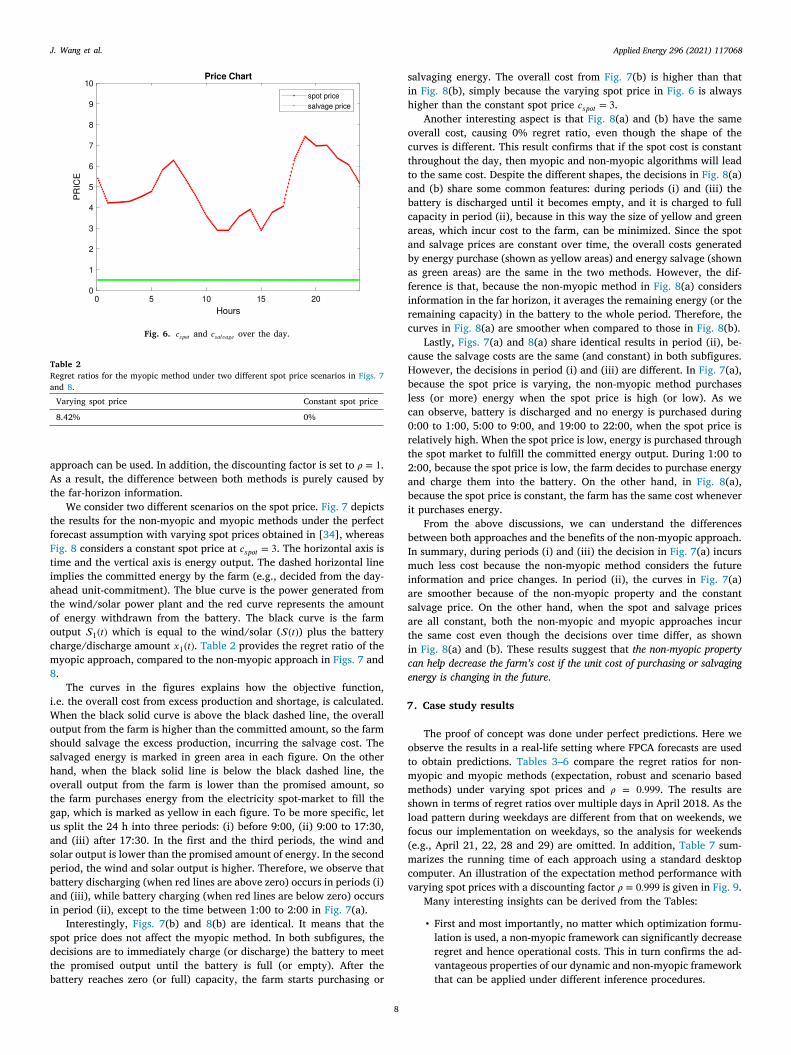
Applied Energy 296 (2021) 117068J. Wang et al.
At
tfFtiatoocm8
iWosshotguaspbai
sdtb
Fig. 6. 𝑐𝑠𝑝𝑜𝑡 and 𝑐𝑠𝑎𝑙𝑣𝑎𝑔𝑒 over the day.
Table 2Regret ratios for the myopic method under two different spot price scenarios in Figs. 7and 8.
Varying spot price Constant spot price
8.42% 0%
approach can be used. In addition, the discounting factor is set to 𝜌 = 1.s a result, the difference between both methods is purely caused by
he far-horizon information.We consider two different scenarios on the spot price. Fig. 7 depicts
he results for the non-myopic and myopic methods under the perfectorecast assumption with varying spot prices obtained in [34], whereasig. 8 considers a constant spot price at 𝑐𝑠𝑝𝑜𝑡 = 3. The horizontal axis isime and the vertical axis is energy output. The dashed horizontal linemplies the committed energy by the farm (e.g., decided from the day-head unit-commitment). The blue curve is the power generated fromhe wind/solar power plant and the red curve represents the amountf energy withdrawn from the battery. The black curve is the farmutput 𝑆1(𝑡) which is equal to the wind/solar (𝑆(𝑡)) plus the batteryharge/discharge amount 𝑥1(𝑡). Table 2 provides the regret ratio of theyopic approach, compared to the non-myopic approach in Figs. 7 and.
The curves in the figures explains how the objective function,.e. the overall cost from excess production and shortage, is calculated.
hen the black solid curve is above the black dashed line, the overallutput from the farm is higher than the committed amount, so the farmhould salvage the excess production, incurring the salvage cost. Thealvaged energy is marked in green area in each figure. On the otherand, when the black solid line is below the black dashed line, theverall output from the farm is lower than the promised amount, sohe farm purchases energy from the electricity spot-market to fill theap, which is marked as yellow in each figure. To be more specific, lets split the 24 h into three periods: (i) before 9:00, (ii) 9:00 to 17:30,nd (iii) after 17:30. In the first and the third periods, the wind andolar output is lower than the promised amount of energy. In the seconderiod, the wind and solar output is higher. Therefore, we observe thatattery discharging (when red lines are above zero) occurs in periods (i)nd (iii), while battery charging (when red lines are below zero) occursn period (ii), except to the time between 1:00 to 2:00 in Fig. 7(a).
Interestingly, Figs. 7(b) and 8(b) are identical. It means that thepot price does not affect the myopic method. In both subfigures, theecisions are to immediately charge (or discharge) the battery to meethe promised output until the battery is full (or empty). After theattery reaches zero (or full) capacity, the farm starts purchasing or
8
salvaging energy. The overall cost from Fig. 7(b) is higher than thatin Fig. 8(b), simply because the varying spot price in Fig. 6 is alwayshigher than the constant spot price 𝑐𝑠𝑝𝑜𝑡 = 3.
Another interesting aspect is that Fig. 8(a) and (b) have the sameoverall cost, causing 0% regret ratio, even though the shape of thecurves is different. This result confirms that if the spot cost is constantthroughout the day, then myopic and non-myopic algorithms will leadto the same cost. Despite the different shapes, the decisions in Fig. 8(a)and (b) share some common features: during periods (i) and (iii) thebattery is discharged until it becomes empty, and it is charged to fullcapacity in period (ii), because in this way the size of yellow and greenareas, which incur cost to the farm, can be minimized. Since the spotand salvage prices are constant over time, the overall costs generatedby energy purchase (shown as yellow areas) and energy salvage (shownas green areas) are the same in the two methods. However, the dif-ference is that, because the non-myopic method in Fig. 8(a) considersinformation in the far horizon, it averages the remaining energy (or theremaining capacity) in the battery to the whole period. Therefore, thecurves in Fig. 8(a) are smoother when compared to those in Fig. 8(b).
Lastly, Figs. 7(a) and 8(a) share identical results in period (ii), be-cause the salvage costs are the same (and constant) in both subfigures.However, the decisions in period (i) and (iii) are different. In Fig. 7(a),because the spot price is varying, the non-myopic method purchasesless (or more) energy when the spot price is high (or low). As wecan observe, battery is discharged and no energy is purchased during0:00 to 1:00, 5:00 to 9:00, and 19:00 to 22:00, when the spot price isrelatively high. When the spot price is low, energy is purchased throughthe spot market to fulfill the committed energy output. During 1:00 to2:00, because the spot price is low, the farm decides to purchase energyand charge them into the battery. On the other hand, in Fig. 8(a),because the spot price is constant, the farm has the same cost wheneverit purchases energy.
From the above discussions, we can understand the differencesbetween both approaches and the benefits of the non-myopic approach.In summary, during periods (i) and (iii) the decision in Fig. 7(a) incursmuch less cost because the non-myopic method considers the futureinformation and price changes. In period (ii), the curves in Fig. 7(a)are smoother because of the non-myopic property and the constantsalvage price. On the other hand, when the spot and salvage pricesare all constant, both the non-myopic and myopic approaches incurthe same cost even though the decisions over time differ, as shownin Fig. 8(a) and (b). These results suggest that the non-myopic propertycan help decrease the farm’s cost if the unit cost of purchasing or salvagingenergy is changing in the future.
7. Case study results
The proof of concept was done under perfect predictions. Here weobserve the results in a real-life setting where FPCA forecasts are usedto obtain predictions. Tables 3–6 compare the regret ratios for non-myopic and myopic methods (expectation, robust and scenario basedmethods) under varying spot prices and 𝜌 = 0.999. The results areshown in terms of regret ratios over multiple days in April 2018. As theload pattern during weekdays are different from that on weekends, wefocus our implementation on weekdays, so the analysis for weekends(e.g., April 21, 22, 28 and 29) are omitted. In addition, Table 7 sum-marizes the running time of each approach using a standard desktopcomputer. An illustration of the expectation method performance withvarying spot prices with a discounting factor 𝜌 = 0.999 is given in Fig. 9.
Many interesting insights can be derived from the Tables:
• First and most importantly, no matter which optimization formu-lation is used, a non-myopic framework can significantly decreaseregret and hence operational costs. This in turn confirms the ad-vantageous properties of our dynamic and non-myopic framework
that can be applied under different inference procedures.
Applied Energy 296 (2021) 117068J. Wang et al.
(
Fig. 7. Results with varying spot prices and no discounting factor, i.e. 𝜌 = 1, under perfect forecast.
Fig. 8. Results with constant spot prices and no discounting factor, i.e. 𝜌 = 1, under perfect forecast.
• Second, interestingly, we observe that the scenario-based ap-proach is able to slightly outperform the expectation-based ap-proach when the number of scenarios is large. This is intuitivelyunderstandable because it can account for prediction uncertaintywith multiple scenarios (rather than using one expected tra-jectory in the expectation-based approach) within our decisionframework. The caveat, however, is that accounting for such un-certainty comes at the expense of increased computational times.For instance, the running time to make storage decisions increasesfrom around 2.4 min to 28 min (refer to Table 7) when switchingfrom expectation-based formulation to the scenario-based formu-lation with 10 scenarios. For the 5-min time interval considered inthis study, Scenario-10 is hence an unfeasible option. We can alsoimagine that the scenarios-based approach is not scalable to solvelarge-scale problems with multiple renewables and batteries.
• Third, the Robust approach leads to worst case regret. This is ex-pected, as we are taking decisions under worst case supply scenar-ios. The Robust approach provides very conservative decisions,increasing operational costs.
• Finally, from these results, while the proposed framework isflexible enough to include different optimization formulations,the expectation approach appears to be most adequate in termsof operational cost and running time.
Fig. 9 also echoes our results. Through comparing Fig. 9(a) and
9
b), we observe the benefit of far-horizon planning where in period
(i), the farm purchases more energy when the spot price is low anduses it when the spot price is high. This results in a smaller regret (orcost), compared to the myopic approach (see Tables 3 and 4). Also,in comparison with the non-myopic approach under perfect forecast(Fig. 7(a)), we find that the major difference happens in period (ii),where the salvaging happens only in the later part of the period inFig. 9(a). This difference is due to the use of a discount factor in thissetting. Since, the unit cost of salvaged energy is 𝜌𝑡−𝑡0 𝑐𝑠𝑎𝑙𝑣𝑎𝑔𝑒, which isdecreasing over time 𝑡. Thus, in period (ii), the farm prefers to salvageits excess energy later, when the unit cost is lower.
8. Conclusion
This paper presents a practical and easy to implement methodologyfor managing the output of a wind/solar farm in a cost effective andreal-time manner. Our problem aims at deciding the amount of energycharged into, or withdrawn from, a battery, considering the time-varying nature in the renewable energy output. A salient aspect of ourformulation is that it enables real-time updating of a joint predictive–prescriptive model where forecasts of energy outputs over the futurehorizon are used to update decisions. This scheme is enabled viaFPCA which accounts for data heterogeneity, safeguards against modelmis-specification via non-parametric predictions, and features a lineardecomposition which in turn enables efficient real-time updating. Weshow that our scheme is flexible to different optimization schemes; be
it stochastic, robust or even a deterministic approach. Our technology
Applied Energy 296 (2021) 117068J. Wang et al.
TN(
0
Fig. 9. Results with varying spot prices and a discounting factor 𝜌 = 0.999.
able 3on-myopic approach: regret ratio with varying spot prices and discounting factor𝜌 = 0.999).Non-myopic Expectation Scenario Scenario Scenarioapproach 2 5 10
Apr 17, 2018 9.35% 10.62% 9.34% 7.93%Apr 18, 2018 1.76% 1.75% 1.39% 1.26%Apr 19, 2018 15.01% 16.79% 13.77% 12.98%Apr 20, 2018 12.16% 13.12% 10.80% 10.38%Apr 23, 2018 3.65% 4.08% 3.42% 3.37%Apr 24, 2018 6.01% 6.57% 5.21% 5.11%Apr 25, 2018 7.11% 8.30% 6.22% 6.17%Apr 26, 2018 6.22% 9.88% 7.15% 5.31%Apr 27, 2018 6.45% 10.25% 7.60% 5.92%Apr 30, 2018 4.38% 7.06% 5.67% 4.93%
Average 7.21% 8.84% 7.06% 6.34%
Table 4Myopic approach: regret ratio with varying spot prices and discounting factor (𝜌 =.999).Myopic Expectation Scenario Scenario Scenarioapproach 2 5 10
Apr 17, 2018 10.46% 10.36% 10.36% 10.36%Apr 18, 2018 9.70% 10.03% 9.77% 9.70%Apr 19, 2018 14.53% 14.81% 14.59% 14.56%Apr 20, 2018 18.34% 18.61% 18.42% 18.52%Apr 23, 2018 9.47% 9.56% 9.48% 9.53%Apr 24, 2018 13.13% 12.94% 12.90% 13.01%Apr 25, 2018 10.56% 10.56% 10.53% 10.53%Apr 26, 2018 11.08% 11.37% 11.17% 11.18%Apr 27, 2018 10.11% 10.34% 10.02% 10.20%Apr 30, 2018 10.69% 10.74% 10.77% 10.73%
Average 11.81% 11.93% 11.82% 11.83%
is then tested on the California ISO dataset [33]. This case studyprovided a proof-of-concept that highlights both the benefits and easeof implementation of our forward looking framework.
Our model can be extended in various directions. For instance,one may consider the battery degradation over time by providing apredictive model to update the capacity limits, much like how FPCA ispredicting supply. In addition, planning decisions for optimal neededbattery capacity is an important problem, in particular, with largepenetration of volatile renewable energy in the electricity market. Sucha problem might benefit from a non-myopic approach such as ours,especially since FPCA can handle both short and long term predictionsas long as all historical and to-be predicted functions share the samedomain. We hope to work on such challenges in the future.
10
Table 5Non-myopic approach: regret ratio with varying spot prices and discounting factor(𝜌 = 0.999).
Non-myopic Expectation Robust Robust Robustapproach 2 5 10
Apr 17, 2018 9.35% 10.48% 10.49% 10.45%Apr 18, 2018 1.76% 10.05% 10.05% 10.24%Apr 19, 2018 15.01% 14.61% 14.82% 14.81%Apr 20, 2018 12.16% 18.64% 18.55% 18.82%Apr 23, 2018 3.65% 9.53% 9.73% 9.71%Apr 24, 2018 6.01% 13.10% 13.54% 13.51%Apr 25, 2018 7.11% 10.27% 10.65% 10.77%Apr 26, 2018 6.22% 11.34% 11.65% 11.74%Apr 27, 2018 6.45% 10.33% 10.53% 10.56%Apr 30, 2018 4.38% 10.81% 10.85% 10.91%
Average 7.21% 11.95% 12.09% 12.15%
Table 6Myopic approach: regret ratio with varying spot prices and discounting factor (𝜌 =0.999).
Myopic Expectation Robust Robust Robustapproach 2 5 10
Apr 17, 2018 10.46% 10.42% 10.57% 10.53%Apr 18, 2018 9.70% 9.86% 9.76% 9.82%Apr 19, 2018 14.53% 14.48% 14.40% 14.37%Apr 20, 2018 18.34% 18.69% 18.61% 18.57%Apr 23, 2018 9.47% 9.45% 9.48% 9.48%Apr 24, 2018 13.13% 12.84% 12.88% 12.91%Apr 25, 2018 10.56% 10.54% 10.50% 10.56%Apr 26, 2018 11.08% 11.06% 11.07% 11.07%Apr 27, 2018 10.11% 10.19% 10.18% 10.16%Apr 30, 2018 10.69% 10.68% 10.72% 10.69%
Average 11.81% 11.82% 11.82% 11.82%
Table 7Average computational time for all approaches.
Proposed methods Running time (s)
Myopic Non-Myopic
Expectation 0.001 145.21Scenario 2 2.07 60.16Scenario 5 2.10 332.92Scenario 10 2.37 1676.10Robust 2 2.26 73.85Robust 5 2.42 428.36Robust 10 2.66 2199.4
Applied Energy 296 (2021) 117068J. Wang et al.
dsfto
A
m
O
A
OltpsWoooa
R
CRediT authorship contribution statement
Jingxing Wang: Played a key role in developing the optimizationframework and running simulations/case studies. Seokhyun Chung:Played a key role in developing the predictive framework and runningsimulations/case studies. Abdullah AlShelahi: Played a key role ineveloping the optimization framework and running simulations/casetudies. Raed Kontar: Played a key role in developing the predictiveramework. Eunshin Byon: Played a key role in developing the predic-ive framework. Romesh Saigal: Played a key role in developing theptimization framework.
ppendix A. Robust approach
in max𝑖
{
𝑇−1∑
𝑡=0𝜌𝑡 ⋅ [𝑐𝑠𝑎𝑙𝑣𝑎𝑔𝑒(𝑡) ⋅ (𝑂(𝑖)
𝑒𝑥𝑐𝑒𝑠𝑠(𝑡) + 𝑂(𝑖)𝐵 (𝑡))
+𝑐𝑠𝑝𝑜𝑡(𝑡) ⋅ (𝑂(𝑖)𝑠ℎ𝑜𝑟𝑡𝑎𝑔𝑒(𝑡) + 𝑈 (𝑖)
𝐵 (𝑡))] + 𝜌𝑇𝛷(𝐵𝑖(𝑇 ))}
, (25)
In LP formulation,
min𝐹 ,
𝑠.𝑡. 𝐹 ≥𝑇−1∑
𝑡=0𝜌𝑡 ⋅ [𝑐𝑠𝑎𝑙𝑣𝑎𝑔𝑒(𝑡) ⋅ (𝑂(𝑖)
𝑒𝑥𝑐𝑒𝑠𝑠(𝑡) + 𝑂(𝑖)𝐵 (𝑡))
+𝑐𝑠𝑝𝑜𝑡(𝑡) ⋅ (𝑂(𝑖)𝑠ℎ𝑜𝑟𝑡𝑎𝑔𝑒(𝑡) + 𝑈 (𝑖)
𝐵 (𝑡))] + 𝜌𝑇𝛷(𝐵𝑖(𝑇 )) (26)
ther constraints remain the same as scenario-based approach (22).
ppendix B. FPCA considerations
Functional regression methods are often vulnerable in outliers [35].ur FPCA model can also exhibit sensitivity when data contains out-
iers. For example, the Bayesian updating scheme above may leado inaccurate predictions if recent observations stray away from thereviously observed trends. To deal with this issue, we adopt a simpletrategy. First, we smoothen the curves to alleviate local fluctuations.e used a Gaussian kernel smoother in our numerical study, but
ther smoothers can be employed. Next, if an observation lies outsideur 3-sigma prediction interval, we ignore it and wait until the nextbservation to update our model. If ℎ consecutive recent observationsre out of the 3-sigma limits we relax this restriction.
eferences
[1] You M, Byon E, Jin JJ, Lee G. When wind travels through turbines: A new sta-tistical approach for characterizing heterogeneous wake effects in multi-turbinewind farms. IISE Trans 2017;49(1):84–95.
[2] Sixel LM. State mandates for renewables is driving new wind, solar powerprojects. Houston Chronicle 2019. From: https://www.houstonchronicle.com/business/energy/article/State-mandates-for-renewables-is-driving-new-13652699.php#photo-15932105.
[3] Ahmed S, Mahmood A, Hasan A, Sidhu GAS, Butt MFU. A comparative review ofChina, India and Pakistan renewable energy sectors and sharing opportunities.Renew Sustain Energy Rev 2016;57:216–25.
[4] Clastres C, Pham TH, Wurtz F, Bacha S. Ancillary services and optimal householdenergy management with photovoltaic production. Energy 2010;35(1):55–64.
[5] Hesser T, Succar S. Chapter 9-renewables integration through direct load controland demand response smart grid. 2012, p. 209–33.
[6] California Independent System Operator. California ISO home page. 2019, From:http://www.caiso.com/Pages/default.aspx.
[7] Denholm P, O’Connell M, Brinkman G, Jorgenson J. Overgeneration from solarenergy in California. A field guide to the duck chart. Tech. Rep., NationalRenewable Energy Lab.(NREL), Golden, CO (United States); 2015.
[8] California Independent System Operator. Impacts of renewable energy on grid op-erations. 2017, From: https://www.caiso.com/Documents/CurtailmentFastFacts.pdf.
11
[9] Hirth L. The market value of variable renewables: The effect of solar wind powervariability on their relative price. Energy Economics 2013;38:218–36.
[10] Giraud F, Salameh ZM. Steady-state performance of a grid-connected rooftophybrid wind-photovoltaic power system with battery storage. IEEE PowerEngineering Review 2001;21(2):54.
[11] Lambert F. Tesla’s massive powerpack battery in Australia cost $66 million andalready made up to $17 million. Electrek 2018. From: https://electrek.co/2018/09/24/tesla-powerpack-battery-australia-cost-revenue/.
[12] Chandy KM, Low SH, Topcu U, Xu H. A simple optimal power flow model withenergy storage. In: 49th IEEE Conference on Decision and Control (CDC). IEEE;2010, p. 1051–7.
[13] Parisio A, Glielmo L. A mixed integer linear formulation for microgrid eco-nomic scheduling. In: 2011 IEEE International Conference on Smart GridCommunications (SmartGridComm). IEEE; 2011, p. 505–10.
[14] Wang Y, Lin X, Pedram M. Adaptive control for energy storage sys-tems in households with photovoltaic modules. IEEE Trans Smart Grid2014;5(2):992–1001.
[15] He M, Murugesan S, Zhang J. A multi-timescale scheduling approach forstochastic reliability in smart grids with wind generation and opportunisticdemand. IEEE Trans Smart Grid 2013;4(1):521–9.
[16] Neely MJ. Stochastic network optimization with application to communicationand queueing systems. Synthesis Lect Commun Netw 2010;3(1):1–211.
[17] Guo Y, Gong Y, Fang Y, Khargonekar PP, Geng X. Energy and network awareworkload management for sustainable data centers with thermal storage. IEEETrans Parallel Distrib Syst 2013;25(8):2030–42.
[18] Li T, Dong M. Online control for energy storage management with renewableenergy integration. In: 2013 IEEE International Conference on Acoustics, Speechand Signal Processing. IEEE; 2013, p. 5248–52.
[19] Xia S, Ding Z, Du T, Zhang D, Shahidehpour M, Ding T. Multitime scalecoordinated scheduling for the combined system of wind power, photovoltaic,thermal generator, hydro pumped storage, and batteries. IEEE Trans Ind Appl2020;56(3):2227–37.
[20] Li N, Uckun C, Constantinescu EM, Birge JR, Hedman KW, Botterud A. Flexibleoperation of batteries in power system scheduling with renewable energy. IEEETrans Sustain Energy 2015;7(2):685–96.
[21] Uçkun C, Botterud A, Birge JR. An improved stochastic unit commit-ment formulation to accommodate wind uncertainty. IEEE Trans Power Syst2015;31(4):2507–17.
[22] Su W, Wang J, Roh J. Stochastic energy scheduling in microgridswith intermittent renewable energy resources. IEEE Trans Smart Grid2014;5(4):1876–83.
[23] Habib AH, Disfani VR, Kleissl J, de Callafon RA. Market-driven energy stor-age planning for microgrids with renewable energy systems using stochasticprogramming. IFAC-PapersOnLine 2017;50(1):183–8.
[24] Du E, Zhang N, Hodge B-M, Wang Q, Lu Z, Kang C, Kroposki B, Xia Q. Operationof a high renewable penetrated power system with CSP plants: A look-aheadstochastic unit commitment model. IEEE Trans Power Syst 2018;34(1):140–51.
[25] Shuai H, Fang J, Ai X, Wen J, He H. Optimal real-time operation strategy formicrogrid: An ADP-based stochastic nonlinear optimization approach. IEEE TransSustain Energy 2018;10(2):931–42.
[26] Cobos NG, Arroyo JM, Alguacil N, Wang J. Robust energy and reserve schedulingconsidering bulk energy storage units and wind uncertainty. IEEE Trans PowerSyst 2018;33(5):5206–16.
[27] Kim JH, Powell WB. Optimal energy commitments with storage and intermittentsupply. Oper Res 2011;59(6):1347–60.
[28] Salas DF, Powell WB. Benchmarking a scalable approximate dynamic program-ming algorithm for stochastic control of grid-level energy storage. INFORMS JComput 2017;30(1):106–23.
[29] Kwon S, Xu Y, Gautam N. Meeting inelastic demand in systems with storage andrenewable sources. IEEE Trans Smart Grid 2015;8(4):1619–29.
[30] Savkin AV, Khalid M, Agelidis VG. A constrained monotonic charg-ing/discharging strategy for optimal capacity of battery energy storagesupporting wind farms. IEEE Trans Sustain Energy 2016;7(3):1224–31.
[31] Bjork T. Arbitrage Theory in Continuous Time. Oxford University Press; 2009.[32] Yao F, Müller H-G, Wang J-L. Functional data analysis for sparse longitudinal
data. J Amer Statist Assoc 2005;100(470):577–90.[33] California ISO. Production and curtailments data. 2019, From: http://www.caiso.
com/informed/Pages/ManagingOversupply.aspx.[34] Operator CIS. 2019 first quarter report on market issues and performance. 2019,
From: http://www.caiso.com/market/Pages/MarketMonitoring.[35] Hullait H, Leslie DS, Pavlidis NG, King S. Robust function-on-function regression.
Technometrics 2020;1–14.