long-term dynamics in co allowance prices and carbon capture

Long-Term Dynamics in CO2 Allowance Pricesand Carbon Capture Investments

Luis M. AbadieBilbao Bizkaia Kutxa

Gran Vía, 3048009 Bilbao, Spain

E-mail: [email protected]

José M. ChamorroUniversity of the Basque Country

Dpt. Fundamentos del Análisis Económico IAv. Lehendakari Aguirre, 83

48015 Bilbao, SpainE-mail: [email protected]

May 24th 2007

Abstract

In this paper we analyse the behaviour of the EU market for CO2emission allowances; speci�cally, we focus on the contracts maturing inthe Kyoto Protocol�s second period of application (2008 to 2012). Wecalibrate the underlying parameters for the allowance price in the longrun and we also calibrate those from the Spanish wholesale electricitymarket. This information is then used to assess the option to install acarbon capture and storage (CCS) unit in a coal-�red power plant.We use a two-dimensional binomial lattice where costs and pro�ts

are valued and the optimal investment time is determined. In otherwords, we study the trigger allowance prices above which it is optimalto install the capture unit immediately. We further analyse the impactof several variables on the critical prices, among them allowance pricevolatility and a hypothetical government subsidy.We conclude that, at current permit prices, from a �nancial point

of view, immediate installation does not seem justi�ed. This need notbe the case, though, if carbon market parameters change dramaticallyand/or a speci�c policy to promote these units is adopted.Keywords: power plants, European Trading Scheme, Kalman �lter,

carbon capture and storage, real options.JEL Codes:

1

1 INTRODUCTION 2

1 Introduction

Combustion of fossil fuels and other human activities are causing an increasein the atmospheric concentration of greenhouse gases (GHG). This in turninduces climate change with its sequel of a rise in global average temperature.According to Kyoto Protocol, the European Union must reduce its emissionsby 8% below the 1990 levels during 2008 to 2012. In order to ease theful�lment of this commitment, several instruments have been developed.Two of them are the so-called Joint Implementation and Clean DevelopmentMechanisms. The third instrument is the European Trading Scheme (ETS),a system whereby CO2 emission permits are traded.1

The ETS envisages several time phases. The �rst one goes from 2005 to2007 and can be considered as a trial or "warm-up" period. It was precededby an allocation of permits to the installations by the EU Member States;this took place within each country�s National Allocation Plan (NAP). Thesecond allocation phase is planned for the period 2008-2012, which coincideswith the Kyoto commitment period. From then on, succeeding �ve-yearperiods will span the potential post-Kyoto commitment periods.

The trading system started o¢ cially to operate on January 1st 2005.It involves some 4,000 facilities in the EU covering approximately 45% ofCO2 emissions.2 In its initial stage, according to Böhringer et al. [1],free allowance allocation has been a necessary condition for the ETS to beaccepted by carbon-intensive industries with political clout. In spite of this,as Buchner et al. [3] point out, the world�s largest ever market in emissionshas been established, and EU �rms now face a carbon-constrained reality inform of legally binding emission targets.3

European companies thus face the choice between investing in projectsthat help them reduce GHG emissions (so as to incur in lower carbonpayments or get some revenue from spare permits), or purchasing allowancesto release GHG emissions. In this scenario, managers have a pressingneed of project selection methodologies that allow them to sharpen decisionmaking. Some of the issues concerned may be suitably analyzed by meansof standard �nance theory or cost/bene�t analysis. Occasionally, whenmanagers deal with (signi�cantly) irreversible investments, the returns onwhich are (highly) uncertain, and have (non-negligible) �exibility to deferinvestment, real options analysis can prove bene�cial.

Insley [7] addresses the decision faced by an electric power company

1Directive 2003/87/EC establishing a scheme for GHG emission allowance tradingwithin the Community and amending Council Directive 96/61/EC.

2Transport and households, among other sectors, are not covered by the ETS.3As Laurikka and Koljonen [9] point out, emissions trading is likely to impact cash

�ows in a given period through four mechanisms: existing cost categories (fuel costs),new costs (value of surrendered allowances), energy outputs (price of power and heat),additional revenues (free allowances).

1 INTRODUCTION 3

regarding its abatement strategy to comply with the Clean Air Act (theUS Acid Rain Program). In particular, the �rm has the option to install ascrubber to limit sulphur dioxide emissions; if the option is exercised, theneed to purchase emissions permits is eliminated. Obviously, the perceivedbene�t of a scrubber depends on the �rm�s expectations concerning futureallowance prices. The paper considers the e¤ect of uncertainty in the price ofemissions permits on the decision to install the scrubber. This is a problemof investment under uncertainty.4 Speci�cally, the �rm must solve for thedollar value of the investment option as well as for the optimal exercise time,i.e. the optimal time to invest. This takes the form of a "critical" or "trigger"permits price above which the scrubber must be installed immediately;otherwise, it is better to wait and keep the option alive. The paper furtherexamines whether US �rms� actual behaviour is consistent with optimalbehaviour as predicted by the real options model.

Sarkis and Tamarkin [12] consider a project of carbon dioxidere-injection. Sometimes gas extracted from a new �eld contains highCO2 levels that must be removed to comply with pipeline transmissionspeci�cations. Standard practice is to vent this removed CO2 intothe atmosphere. The �rm�s project involves re-injection and long-termunderground storage of CO2 in the reservoir from which the gas wasextracted. Again, the �rm has �exibility to defer installation of the unit untilsome future date. This option to delay has a value; indeed the �rm mustexploit it in such a way that �exibility attains its highest value if the �rm isto maximize its own value. Consequently, as before, the �rm must determinethe optimal time to install the equipment. They use internal estimates fromBritish Petroleum-Amoco (BP) for average carbon price in the coming futureand expected annual growth rate in price. Their conclusion is that, unlesscarbon prices have a dramatic upturn, the installation of this equipmentshould be delayed for an indeterminate time.

Our paper considers the case of an EU-based power company which maypurchase carbon allowances in the ETS in order to release CO2 or mayalternatively install a long-lived carbon capture and storage (CCS) unit. Asusual, the cost of this unit is well known, whereas the future price of thepermits is uncertain. The �rm we have in mind �nds itself in May 2007 butlooks to the future while trying to exploit any source of information aboutit. The ETS plays a crucial role in this respect.

Section 2 provides some background on the market for carbon allowances.Then in Section 3 we propose a stochastic model for the allowance priceand calibrate its parameters from actual ETS data. In particular, weassume a standard geometric Brownian motion and apply Kalman �lter

4Dixit and Pindyck [5] and Trigeorgis [17] provide thorough analyses of the topic.Numerous examples can be found in Brennan and Trigeorgis [2] and Schwarz and Trigeorgis[14].

2 AN OVERVIEW OF CARBON AND ELECTRICITY MARKETS 4

to the price series in order to come up with the underlying dynamics.Concerning electricity price, we assume a mean-reverting stochastic process.Now, though, parameters are calibrated using monthly average prices fromthe Spanish wholesale electricity market (OMEL). Section 4 presents basicparameter values for a Supercritical Pulverized Coal-�red power plant. Thisis the long-lived facility where the potential installation of the CCS unitwould take place. Section 5 shows numerical results. Speci�cally, the optionto install the CCS unit is analyzed alongside the optimal time to invest; asensitivity analysis is also performed. We further consider the possibility ofa government subsidy to promote early adoption of the CCS unit by utilities.Section 6 concludes; under current conditions, it will take many years beforeinvesting in this technology looks �nancially sound.

2 An overview of carbon and electricity markets

2.1 The futures market for emission allowances

In order to accomplish cost-e¢ cient emission reductions, the implementationof the Directive has brought about a regulated market. Contracts onthese emission allowances are traded on di¤erent platforms (in addition toover-the-counter markets). Due to its volume of operations and liquidity, theEuropean Climate Exchange (ECX) stands apart. It manages the EuropeanClimate Exchange Financial Instruments (ECX CFI), which are traded inthe International Petroleum Exchange (IPE). The information on quotesfrom the futures market for emission permits gathered at IPE has been usedhere.

The IPE ECX CPI futures contract is a deliverable contract where eachClearing Member with a position open at cessation of trading for a contractmonth is obliged to make or take delivery of emission allowances to orfrom National Registries in accordance with IPE regulations. Contractswith maturities spanning the next 12 months have been introduced oflate. However, except for those maturing in December, trading is sparse.5

Additionally, 5 December contracts are listed from December 2008 to 2012.Contract size is 1,000 metric ton of carbon dioxide equivalent gas. Priceunits are euros/metric ton. Finally, as usual in futures markets, tradingtakes place continuously and all open contracts are marked-to-market daily.

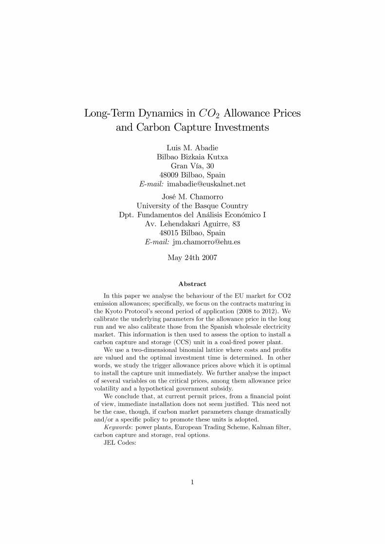
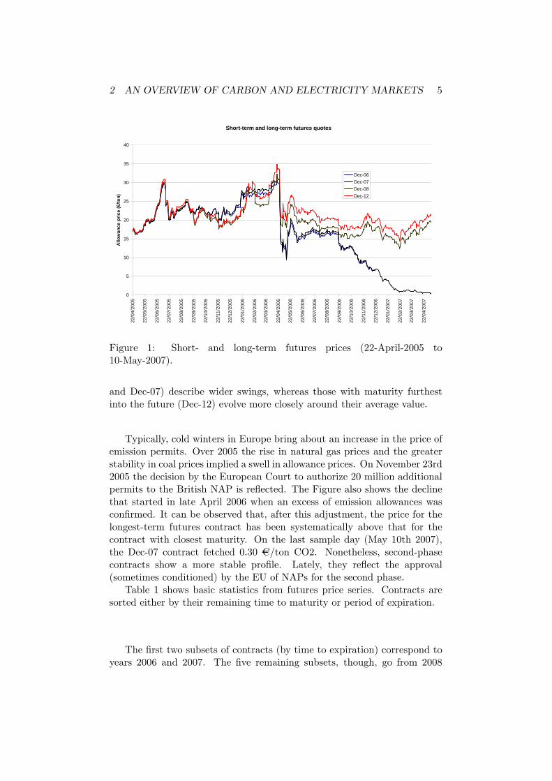
As this paper was developed, there were futures contracts for both the�rst period (2005-2007) and the second one (2008-2012). Figure 1 showsthe lower volatility of long-term futures contracts relative to short-termcontracts. As can be seen, the closest-to-maturity carbon allowances (Dec-06

5Because of their lower liquidity and shorter life span, they do not seem suitable forvaluing long-lived assets and have not been used in this paper. Moreover, they fall withinthe �rst period.


Shortterm and longterm futures quotes

0

5

10

15

20

25

30

35

40

22/0

4/20

05

22/0

5/20

05

22/0

6/20

05

22/0

7/20

05

22/0

8/20

05

22/0

9/20

05

22/1

0/20

05

22/1

1/20

05

22/1

2/20

05

22/0

1/20

06

22/0

2/20

06

22/0

3/20

06

22/0

4/20

06

22/0

5/20

06

22/0

6/20

06

22/0

7/20

06

22/0

8/20

06

22/0

9/20

06

22/1

0/20

06

22/1

1/20

06

22/1

2/20

06

22/0

1/20

07

22/0

2/20

07

22/0

3/20

07

22/0

4/20

07

Allo

wan

ce p

rice

(€/to

n)

Dec06Dec07Dec08Dec12

Figure 1: Short- and long-term futures prices (22-April-2005 to10-May-2007).

and Dec-07) describe wider swings, whereas those with maturity furthestinto the future (Dec-12) evolve more closely around their average value.

Typically, cold winters in Europe bring about an increase in the price ofemission permits. Over 2005 the rise in natural gas prices and the greaterstability in coal prices implied a swell in allowance prices. On November 23rd2005 the decision by the European Court to authorize 20 million additionalpermits to the British NAP is re�ected. The Figure also shows the declinethat started in late April 2006 when an excess of emission allowances wascon�rmed. It can be observed that, after this adjustment, the price for thelongest-term futures contract has been systematically above that for thecontract with closest maturity. On the last sample day (May 10th 2007),the Dec-07 contract fetched 0.30 AC/ton CO2. Nonetheless, second-phasecontracts show a more stable pro�le. Lately, they re�ect the approval(sometimes conditioned) by the EU of NAPs for the second phase.

Table 1 shows basic statistics from futures price series. Contracts aresorted either by their remaining time to maturity or period of expiration.

The �rst two subsets of contracts (by time to expiration) correspond toyears 2006 and 2007. The �ve remaining subsets, though, go from 2008


Table 1. Summary statistics for CO2 emission allowances (2006-2012).Daily data from 01-05-2006 to 10-05-2007

Price (AC/ton) Maturity (years)Futures Observations Mean Std. Deviation Mean Std. DeviationContracts 1,755 16.80 4.80 3.31 1.92

Grouped by time to maturity1. Dec-06 165 13.67 3.29 0.32 0.182. Dec-07 265 9.58 6.56 1.12 0.303. Dec-08 265 17.49 2.19 2.12 0.304. Dec-09 265 18.06 2.21 3.11 0.305. Dec-10 265 18.63 2,23 4.13 0.306. Dec-11 265 19.20 2.26 5.13 0.307. Dec-12 265 19.77 2.28 6.12 0.30

Grouped by period2006-2007 430 11.15 5.88 0.81 0.472008-2012 1,325 18.63 2.37 4.12 1.45

to 2012. It can be seen that the average futures price increases mildlywith time to maturity. Concerning price volatility, it rises within each ofthe two implementation subperiods as the term of the contracts lengthens.This pattern is hardly consistent with mean reversion in prices. 6 Also,volatility drops signi�cantly from the �rst subperiod to the second, beingmuch lower for futures contracts expiring from 2008 to 2012. One possibleexplanation is that short-term behaviour is mainly driven by current NAPswhich are known for certain, while there is greater scope for uncertainty inthe post-2008 scenario.7

Yet it is the second period (2008-2012) which seems to be more suitableto assess long-run dynamics in allowance prices, given that we deal with thevaluation of long-lived assets. Also, the structural change shown in Figure1 suggests the convenience to use exclusively the second period for long-runestimations and only from May 2006 onwards. Thus Table 1 shows basicstatistics for the futures price series starting on May 1st 2006. We thushave 1,325 daily obervations for 5 futures contracts maturing from Dec-08to Dec-12. As already mentioned, the increasing relation between volatilityand maturity advances the geometric Brownian motion as a suitable modelfor allowance price.

6 Indeed, it is the opposite of observed patterns in many commodities futures marketswhich display the �Samuelson e¤ect�, a sign of mean reversion.

7Under the ETS, utilities have received at least 95% of the allocated permits for2005-2007 free of charge. For 2008-2012, this percentage drops to 90%.


Evolution of the average monthly price of electricity

0

1.000

2.000

3.000

4.000

5.000

6.000

7.000

8.000

1998

01

1998

05

1998

09

1999

01

1999

05

1999

09

2000

01

2000

05

2000

09

2001

01

2001

05

2001

09

2002

01

2002

05

2002

09

2003

01

2003

05

2003

09

2004

01

2004

05

2004

09

2005

01

2005

05

2005

09

2006

01

2006

05

2006

09

2007

01

Pri

ce (c

ent.

€/K

wh)

Average monthly price OMEL market

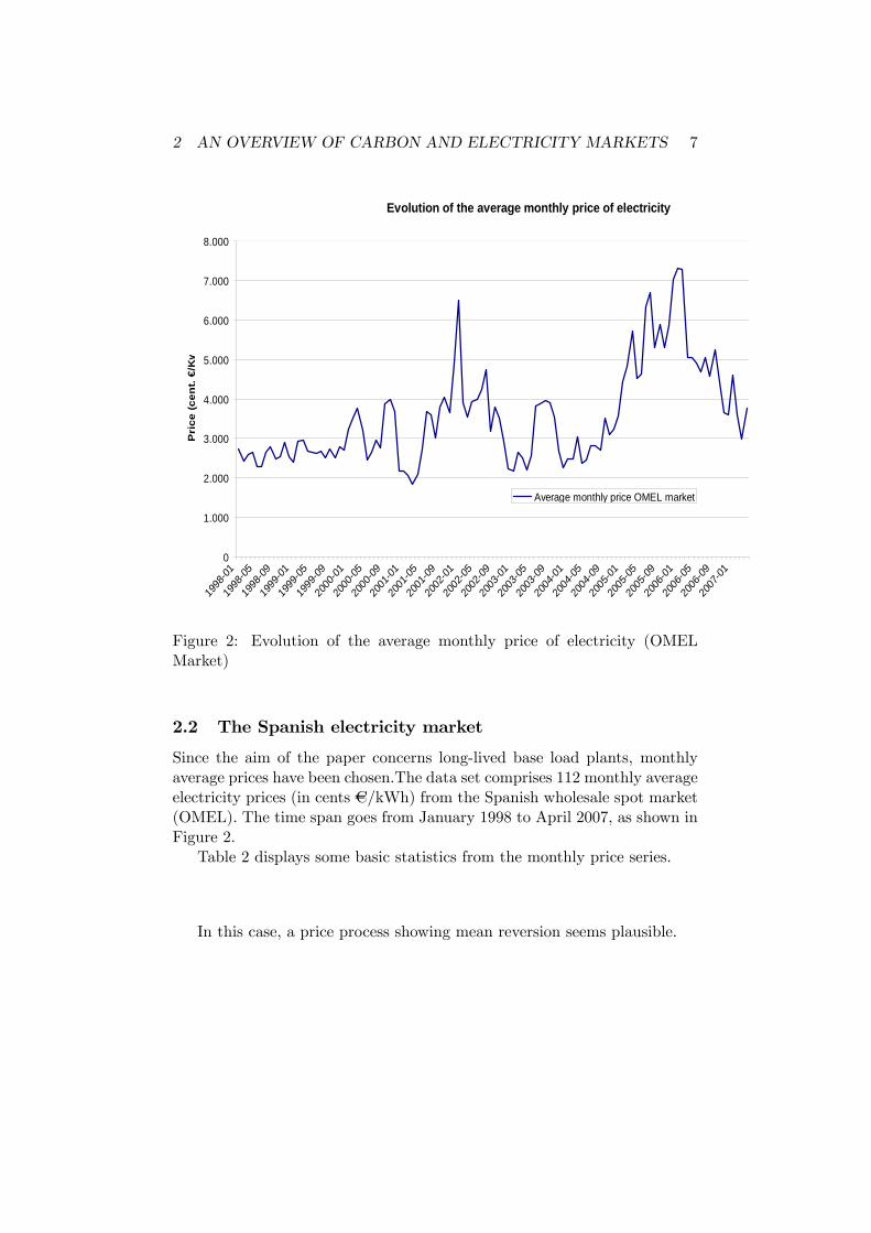
Figure 2: Evolution of the average monthly price of electricity (OMELMarket)

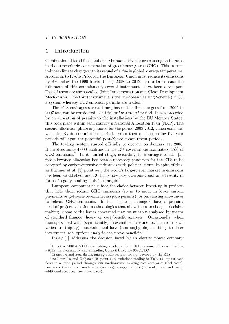
2.2 The Spanish electricity market

Since the aim of the paper concerns long-lived base load plants, monthlyaverage prices have been chosen.The data set comprises 112 monthly averageelectricity prices (in cents AC/kWh) from the Spanish wholesale spot market(OMEL). The time span goes from January 1998 to April 2007, as shown inFigure 2.

Table 2 displays some basic statistics from the monthly price series.

In this case, a price process showing mean reversion seems plausible.

3 STOCHASTIC MODELS AND PARAMETER VALUES 8

Table 2. Statistics from OMEL market.Mean (cts AC/kWh) 3.5504

Median 3.2165Minimum 1.8250Maximum 7.3140

Standard deviation 1.2351Coe¤. Variation 0.34788

Skewness 1.1447Excess Kurtosis 0.84177

3 Stochastic models and parameter values

3.1 The model for emission allowance price

We assume that the CO2 allowance price follows a non-stationary stochasticprocess. Speci�cally, following Insley [7], it is governed by a GeometricBrownian Motion (GBM):8

dCt = �cCtdt+ �cCtdWct ; (1)

where Ct denotes the time-t (spot) price of the allowance to emit 1 tonneof CO2, and E(Ct) = C0e�ct. Adopting the transformation Xt � lnCt andapplying Ito�s Lemma yields:

dXt = (�c ��2c2)dt+ �cdW

ct : (2)

The risk-neutral version of this equation is:

dXt = (�c ��2c2� �)dt+ �cdW c

t ; (3)

where � stands for the risk premium.Now, the futures price F (�) (in euros/ton CO2), i.e. the value of the

delivery price at time t such that the current value of the futures contractequals zero, is the expected spot price in a risk-neutral context. Besides, bythe properties of the log-normal distribution (X) we know that:

F (C0;t) = e(E(X)+ 1

2V ar(X)) = e(lnC0+(�c�

�2

2��)t+�2

2t) = C0e

(�c��)t: (4)

Stating the equation in logarithmic form we get:

lnF (C0;t) = lnC0 + (�c � �)t: (5)

8 Instead, Laurikka [8] assumes a one-factor mean-reverting process, namely theOrnstein-Uhlenbeck process.


We are going to estimate the parameters of this process by applyingKalman �lter. The measure equation is deduced from equation (4) sincewe observe futures quotes, whereas the unobservable spot price is the statevariable. Therefore, using Harvey�s [6] notation, for the measure equation:

yt = Zt�t + dt + "t; t = 1; 2; :::; T

where:a) yt = [lnF (tNt )]; N = 1; 2; :::; 5; vector of observations (contract price

series).b) Zt is an N�m matrix, N being the number of futures prices available

for each day, and m = 1 being the number of state variables (just one inthis case, namely the spot price). We thus have Zt = [1 1 1 1 1]0:

c) �t � Xt is the non-observable state variable on each day.d) dt is a 5� 1 matrix of the form:

dt �

0@ (�c � �)t1t:::

(�c � �)t5t

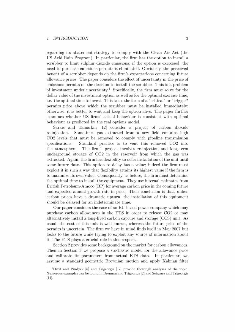
1A ;where t1t is the time to maturity of the closest futures contract at time tt.See Figure 3. This is therefore a Kalman-�lter case in which vector dt variesover time, since the remaining time until the expiration of futures contractschanges from one day to the next.

e) "t is a 5� 1 matrix of serially incorrelated errors. They are assumedto have zero mean and covariance matrix Ht:

E("t) = 0 , V ar("t) = Ht ;

in our case Ht = ��I is chosen, where I denotes the 5� 5 identity matrix.Discretizing equation (2) it is possible to get the transition equation:

Xt+1 �Xt � (�c ��2c2)�t+ �cdW

ct :

In Harvey�s notation:

�t+1 = Tt�t + ct + �t (6)

where �t � Xt; Tt = 1; ct = (�c � �2c2 )�t; E(�t) = 0; V ar(�t) = �

2c�t.

9

Parameter values are derived from maximization of the log-likelihoodfunction; see Table 3.

9Note that an equation of the type dXt = �cdt + �cdWct has as a solution a centered

second moment: [Xt � E(Xt)]2 = �2c

R t0ds = �2c�t:


Futures YESTERDAY (t=0) Futures TODAY (t=1)price price

Time Time

Dec08 Dec09 Dec08 Dec09

t01

t02

t11

t12

Figure 3: Times to maturity of two futures contracts.

Table 3. Parameter values for CO2 allowance prices.Sample period: 01-05-06 to 10-05-07.No. observations 1,325�c 0.0690� 0.0382�c 0.4683�� 0.0056Log-likelihood function 4,324.3

4 BASIC DATA AND PRELIMINARY COMPUTATIONS 11

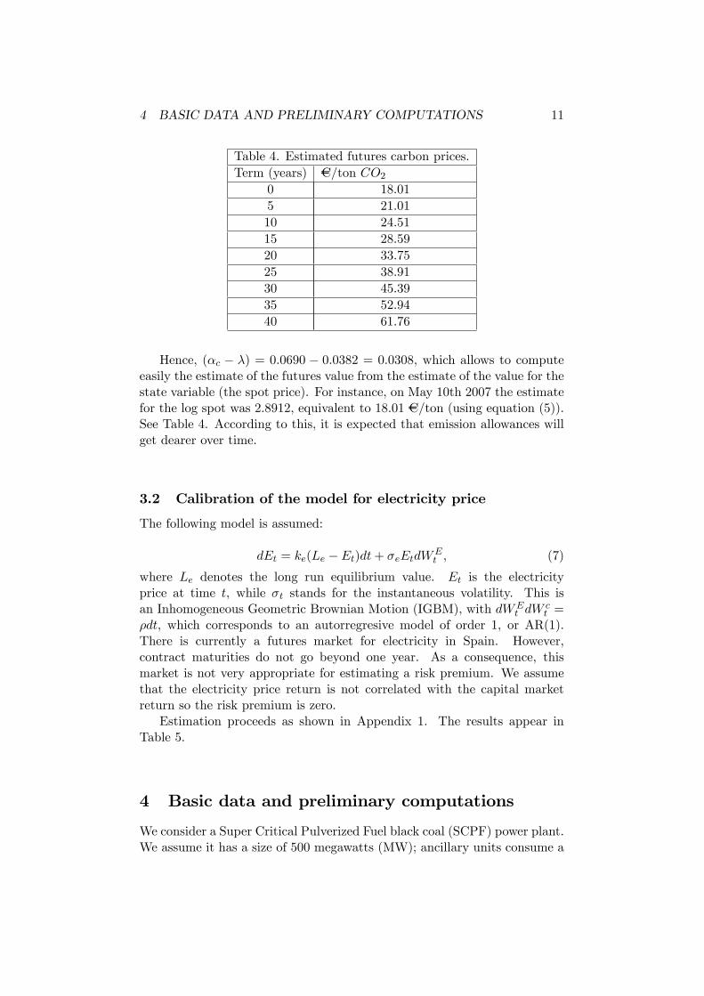
Table 4. Estimated futures carbon prices.Term (years) AC/ton CO2

0 18.015 21.0110 24.5115 28.5920 33.7525 38.9130 45.3935 52.9440 61.76

Hence, (�c � �) = 0:0690 � 0:0382 = 0:0308, which allows to computeeasily the estimate of the futures value from the estimate of the value for thestate variable (the spot price). For instance, on May 10th 2007 the estimatefor the log spot was 2.8912, equivalent to 18.01 AC/ton (using equation (5)).See Table 4. According to this, it is expected that emission allowances willget dearer over time.

3.2 Calibration of the model for electricity price

The following model is assumed:

dEt = ke(Le � Et)dt+ �eEtdWEt ; (7)

where Le denotes the long run equilibrium value. Et is the electricityprice at time t, while �t stands for the instantaneous volatility. This isan Inhomogeneous Geometric Brownian Motion (IGBM), with dWE

t dWct =

�dt, which corresponds to an autorregresive model of order 1, or AR(1).There is currently a futures market for electricity in Spain. However,contract maturities do not go beyond one year. As a consequence, thismarket is not very appropriate for estimating a risk premium. We assumethat the electricity price return is not correlated with the capital marketreturn so the risk premium is zero.

Estimation proceeds as shown in Appendix 1. The results appear inTable 5.

4 Basic data and preliminary computations

We consider a Super Critical Pulverized Fuel black coal (SCPF) power plant.We assume it has a size of 500 megawatts (MW); ancillary units consume a


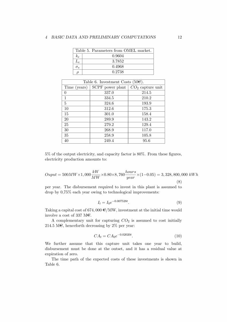
Table 5. Parameters from OMEL market.ke 0.9604Le 3.7852�e 0.4968� 0.2738

Table 6. Investment Costs (MAC).Time (years) SCPF power plant CO2 capture unit0 337.0 214.51 334.5 210.25 324.6 193.910 312.6 175.315 301.0 158.420 289.9 143.225 279.2 129.430 268.9 117.035 258.9 105.840 249.4 95.6

5% of the output electricity, and capacity factor is 80%. From these �gures,electricity production amounts to:

Ouput = 500MW�1; 000 kWMW

�0:80�8; 760hoursyear

�(1�0:05) = 3; 328; 800; 000 kWh(8)

per year. The disbursement required to invest in this plant is assumed todrop by 0,75% each year owing to technological improvements:

It = I0e�0:007528t: (9)

Taking a capital cost of 674; 000 AC/MW, investment at the initial time wouldinvolve a cost of 337 MAC.

A complementary unit for capturing CO2 is assumed to cost initially214.5 MAC, henceforth decreasing by 2% per year:

CAt = CA0e�0:02020t: (10)

We further assume that this capture unit takes one year to build,disbursement must be done at the outset, and it has a residual value atexpiration of zero.

The time path of the expected costs of these investments is shown inTable 6.


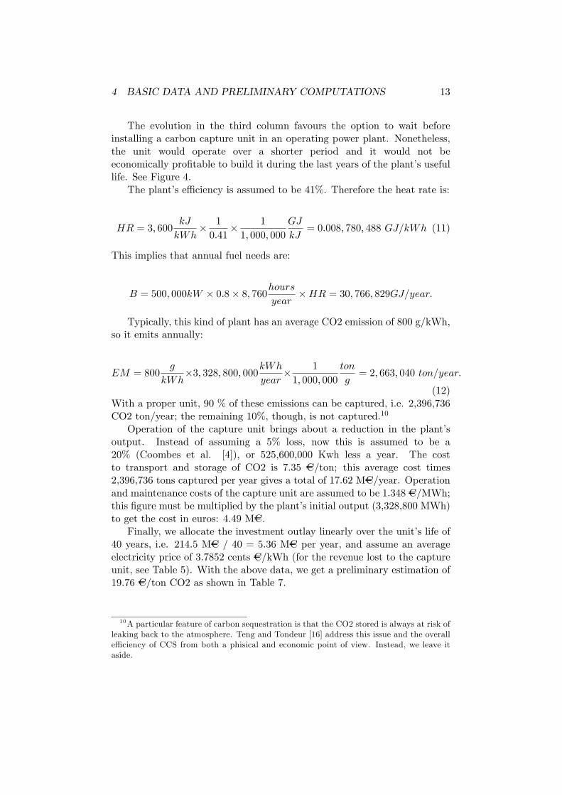
The evolution in the third column favours the option to wait beforeinstalling a carbon capture unit in an operating power plant. Nonetheless,the unit would operate over a shorter period and it would not beeconomically pro�table to build it during the last years of the plant�s usefullife. See Figure 4.

The plant�s e¢ ciency is assumed to be 41%. Therefore the heat rate is:

HR = 3; 600kJ

kWh� 1

0:41� 1

1; 000; 000

GJ

kJ= 0:008; 780; 488 GJ=kWh (11)

This implies that annual fuel needs are:

B = 500; 000kW � 0:8� 8; 760hoursyear

�HR = 30; 766; 829GJ=year:

Typically, this kind of plant has an average CO2 emission of 800 g/kWh,so it emits annually:

EM = 800g

kWh�3; 328; 800; 000kWh

year� 1

1; 000; 000

ton

g= 2; 663; 040 ton=year:

(12)With a proper unit, 90 % of these emissions can be captured, i.e. 2,396,736CO2 ton/year; the remaining 10%, though, is not captured.10

Operation of the capture unit brings about a reduction in the plant�soutput. Instead of assuming a 5% loss, now this is assumed to be a20% (Coombes et al. [4]), or 525,600,000 Kwh less a year. The costto transport and storage of CO2 is 7.35 AC/ton; this average cost times2,396,736 tons captured per year gives a total of 17.62 MAC/year. Operationand maintenance costs of the capture unit are assumed to be 1.348 AC/MWh;this �gure must be multiplied by the plant�s initial output (3,328,800 MWh)to get the cost in euros: 4.49 MAC.

Finally, we allocate the investment outlay linearly over the unit�s life of40 years, i.e. 214.5 MAC / 40 = 5.36 MAC per year, and assume an averageelectricity price of 3.7852 cents AC/kWh (for the revenue lost to the captureunit, see Table 5). With the above data, we get a preliminary estimation of19.76 AC/ton CO2 as shown in Table 7.

10A particular feature of carbon sequestration is that the CO2 stored is always at risk ofleaking back to the atmosphere. Teng and Tondeur [16] address this issue and the overalle¢ ciency of CCS from both a phisical and economic point of view. Instead, we leave itaside.


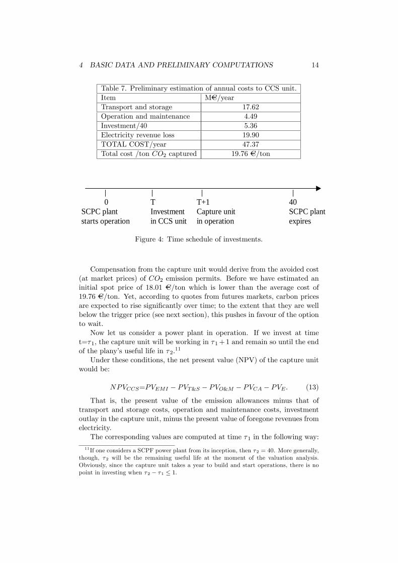
Table 7. Preliminary estimation of annual costs to CCS unit.Item MAC/yearTransport and storage 17.62Operation and maintenance 4.49Investment/40 5.36Electricity revenue loss 19.90TOTAL COST/year 47.37Total cost /ton CO2 captured 19.76 AC/ton

0 T T+1 40SCPC plant Investment Capture unit SCPC plantstarts operation in CCS unit in operation expires

Figure 4: Time schedule of investments.

Compensation from the capture unit would derive from the avoided cost(at market prices) of CO2 emission permits. Before we have estimated aninitial spot price of 18.01 AC/ton which is lower than the average cost of19.76 AC/ton. Yet, according to quotes from futures markets, carbon pricesare expected to rise signi�cantly over time; to the extent that they are wellbelow the trigger price (see next section), this pushes in favour of the optionto wait.

Now let us consider a power plant in operation. If we invest at timet=�1, the capture unit will be working in �1+1 and remain so until the endof the plany�s useful life in �2.11

Under these conditions, the net present value (NPV) of the capture unitwould be:

NPVCCS=PVEMI � PVT&S � PVO&M � PVCA � PVE : (13)

That is, the present value of the emission allowances minus that oftransport and storage costs, operation and maintenance costs, investmentoutlay in the capture unit, minus the present value of foregone revenues fromelectricity.

The corresponding values are computed at time �1 in the following way:

11 If one considers a SCPF power plant from its inception, then �2 = 40. More generally,though, �2 will be the remaining useful life at the moment of the valuation analysis.Obviously, since the capture unit takes a year to build and start operations, there is nopoint in investing when �2 � �1 � 1:


PVEMI = EM0e�2(�c��c�r) � e(�1+1)(�c��c�r)

(�c � �c � r); (14)

where EM0 = 2; 396; 736 ton=year � 18:01 AC=ton = 43:165 MAC.

PVT&S = TA0e�r(�1+1) � e��2r

r; (15)

where TA0 = 17:62 MAC.

PVO&M = OM0e�r(�1+1) � e��2r

r; (16)

where OM0 = 4:49 MAC.

PVCA = CA0e�0:02020T ;

where CA0 = 214:5 MAC.

PVE = PA0[Ler(e�r(T+1)�e�40r)+( E0

ke + r� Leke + r

)(e�(ke+r)(T+1)�e�40(ke+r))](17)

where PA0 = 525; 600; 000 kWh/year lost, Le = 0:037852 AC/kWh, E0 =0:04083 AC/kWh (as of April 2007, deseasonalised), ke = 0:9604 and r = 0:05:

With these values, initially, if the decision to install a capture unit weretaken (which would operate in one years�s time), the NPV would be:

NPVCCS = 1; 162:40� 287:45� 73:21� 214:50� 325:20 == 262:04 MAC.

Thus, following the NPV criterion investment at that time would beaccomplished.12

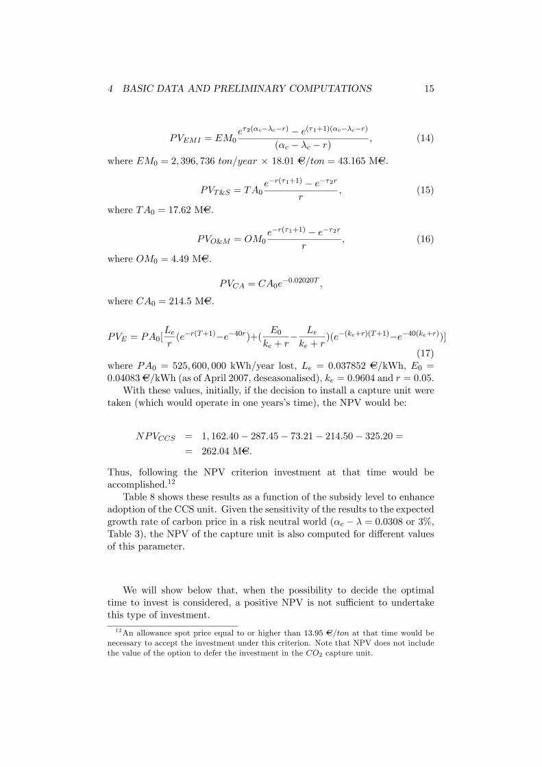
Table 8 shows these results as a function of the subsidy level to enhanceadoption of the CCS unit. Given the sensitivity of the results to the expectedgrowth rate of carbon price in a risk neutral world (�c � � = 0:0308 or 3%,Table 3), the NPV of the capture unit is also computed for di¤erent valuesof this parameter.

We will show below that, when the possibility to decide the optimaltime to invest is considered, a positive NPV is not su¢ cient to undertakethis type of investment.12An allowance spot price equal to or higher than 13:95 AC=ton at that time would be

necessary to accept the investment under this criterion. Note that NPV does not includethe value of the option to defer the investment in the CO2 capture unit.

5 NUMERICAL RESULTS 16

Table 8. NPV of the capture unit (MAC) with varying subsidies(Investment outlay = 214.5 MAC)

Subsidy (%) �c � � = 0:01 �c � � = 0:02 �c � � = 0:03080 -81.43 62.57 262.0410 -59.98 84.02 283.4920 -38.53 105.47 304.9430 -17.08 126.92 326.3940 4.37 148.37 347.8450 25.82 169.82 369.2960 47.27 191.27 390.7470 68.72 212.72 412.1980 90.17 234.17 433.6490 111.62 255.62 455.09100 133.07 277.07 476.54

5 Numerical results

5.1 Binomial Lattice for the risk-neutral GBM and IGBMprocesses

We have two risk-neutral stochastic processes. For the carbon allowanceprice:

dXt = (�c ��2c2� �)dt+ �cdW c

t = �1dt+ �cdWct :

For the electricity price, de�ning Yt = lnEt:

dYt = (ke(Le � Et)

Et� �

2e

2)dt+ �edW

Et = �2dt+ �edW

Et ;

with:dW c

t dWEt = �dt:

In order to solve this two-dimensional binomial tree there are fourprobabilities and, if we want the branches to recombine, two incrementvalues (�X and �Y ): Since probabilities must add to one and also beconsistent with means, variances and correlations, there are six restrictionsto be satis�ed. It can be shown that the solution is:

�X = �cp�t; (18)

�Y = �ep�t; (19)

puu =�X�Y +�Y �1�t+�X�2�t+ ��c�e�t

4�X�Y; (20)


pud =�X�Y +�Y �1�t��X�2�t� ��c�e�t

4�X�Y; (21)

pdu =�X�Y ��Y �1�t+�X�2�t� ��c�e�t

4�X�Y; (22)

pdd =�X�Y ��Y �1�t��X�2�t+ ��c�e�t

4�X�Y: (23)

At any time the four probabilities must take on values between zero andone.

A two-dimensional binomial tree is arranged with 6 time steps per year(�t = 1=6). This amounts to 6� 39 =234 steps for the case of 40 years (thelast nodes would occur at time 39, where a null value would arise as themaximum between building the capture unit in exchange for nothing andzero):

W = max(NPVCCS ; 0) = 0 (24)

At earlier moments, in each node the best option is chosen, be it whetherto invest or continue:

W = max(NPVCCS ; (puuW++ + pudW

+� + pduW�+ + pddW

��)e�r�t):(25)

Investing yields the NPVCCS , whereas continuing allows to wait and get thefuture value discounted at the risk-free rate. The future value of the nextstep is the sum of the values in the four nodes weighted by the risk-neutralprobabilities of reaching each of these values.

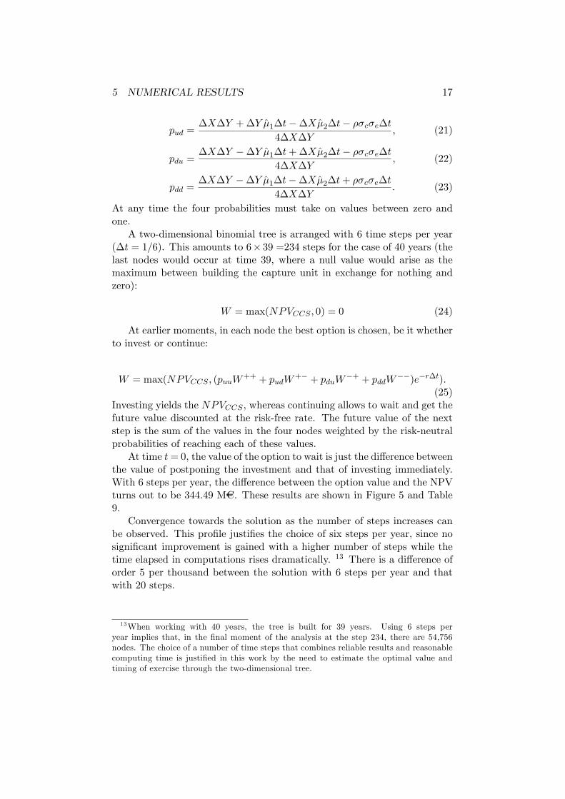
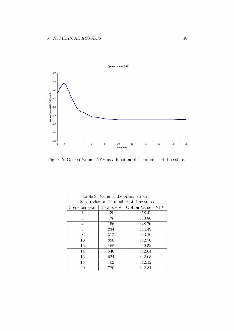
At time t= 0, the value of the option to wait is just the di¤erence betweenthe value of postponing the investment and that of investing immediately.With 6 steps per year, the di¤erence between the option value and the NPVturns out to be 344.49 MAC. These results are shown in Figure 5 and Table9.

Convergence towards the solution as the number of steps increases canbe observed. This pro�le justi�es the choice of six steps per year, since nosigni�cant improvement is gained with a higher number of steps while thetime elapsed in computations rises dramatically. 13 There is a di¤erence oforder 5 per thousand between the solution with 6 steps per year and thatwith 20 steps.

13When working with 40 years, the tree is built for 39 years. Using 6 steps peryear implies that, in the �nal moment of the analysis at the step 234, there are 54,756nodes. The choice of a number of time steps that combines reliable results and reasonablecomputing time is justi�ed in this work by the need to estimate the optimal value andtiming of exercise through the two-dimensional tree.


Option Value NPV

330

335

340

345

350

355

360

365

370

1 2 4 6 8 10 12 14 16 18 20

steps/year

Opt

ion

Valu

e N

PV (m

illio

ns €

)

Figure 5: Option Value - NPV as a function of the number of time steps.

Table 9. Value of the option to wait.Sensitivity to the number of time steps

Steps per year Total steps Option Value - NPV1 39 358.422 78 363.864 156 348.766 234 344.498 312 343.1910 390 342.7012 468 342.5814 546 342.6416 624 342.6318 702 342.1220 780 342.81


Investment and noinvestment regions

0

20

40

60

80

100

120

2 5 10 15 20 25 30 35 40

Remaining useful life of the power plant

Opt

imal

exe

rcis

e pr

ice

(€/to

n)

NPVReal option

Invest

Option Value: No Invest.NPV: Invest

No invest

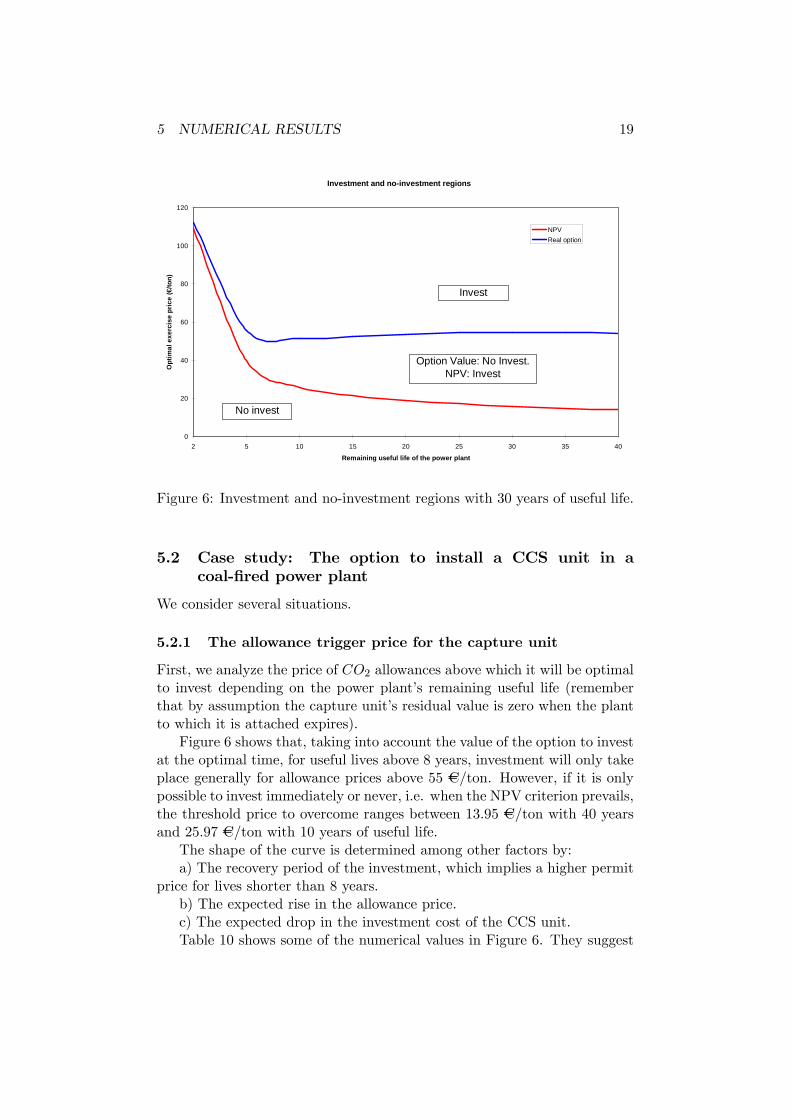
Figure 6: Investment and no-investment regions with 30 years of useful life.

5.2 Case study: The option to install a CCS unit in acoal-�red power plant

We consider several situations.

5.2.1 The allowance trigger price for the capture unit

First, we analyze the price of CO2 allowances above which it will be optimalto invest depending on the power plant�s remaining useful life (rememberthat by assumption the capture unit�s residual value is zero when the plantto which it is attached expires).

Figure 6 shows that, taking into account the value of the option to investat the optimal time, for useful lives above 8 years, investment will only takeplace generally for allowance prices above 55 AC/ton. However, if it is onlypossible to invest immediately or never, i.e. when the NPV criterion prevails,the threshold price to overcome ranges between 13.95 AC/ton with 40 yearsand 25.97 AC/ton with 10 years of useful life.

The shape of the curve is determined among other factors by:a) The recovery period of the investment, which implies a higher permit

price for lives shorter than 8 years.b) The expected rise in the allowance price.c) The expected drop in the investment cost of the CCS unit.Table 10 shows some of the numerical values in Figure 6. They suggest


Table 10. Carbon trigger price as a function of plant�s life.Useful life (years) Real Option NPV

2 112.38 109.005 55.66 39.7510 51.35 25.9715 52.58 21.3920 53.68 18.8425 54.31 17.1130 54.51 15.8135 54.40 14.7940 54.09 13.95

that the current situation is not favourable, from a �nancial point of view,for the �rms to decide to install CCS units right now. Everything pushes fordeferring this type of investments and seeing what happens in the meantime.

One of the most in�uential parameters upon valuation is the allowanceprice volatility. As long as This is high, it is more likely that theseinvestments will be postponed. In the base case we have used an allowanceprice volatility of 46,83% (see Table 3). With 30 years of remaining usefullife, this implies an optimal exercise price of 54.51 AC/ton.

5.2.2 Sensitivity analysis

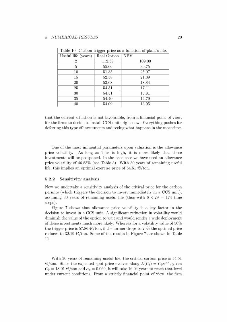
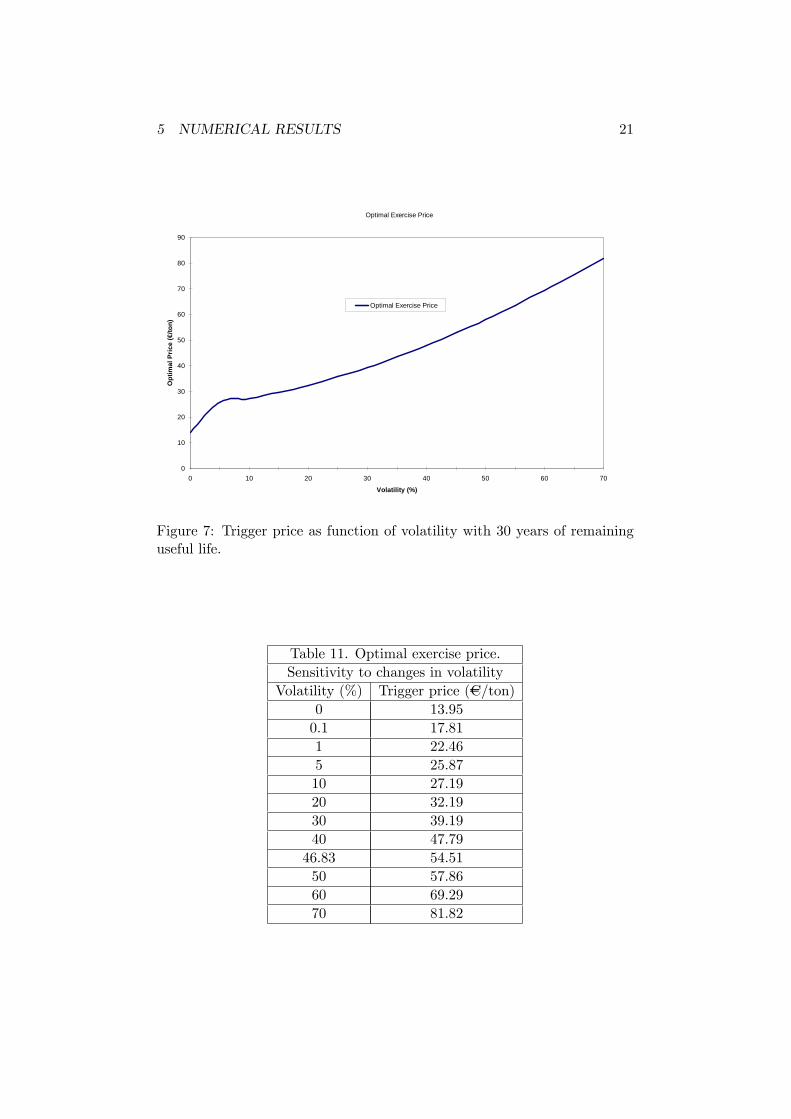
Now we undertake a sensitivity analysis of the critical price for the carbonpermits (which triggers the decision to invest immediately in a CCS unit),assuming 30 years of remaining useful life (thus with 6 � 29 = 174 timesteps).

Figure 7 shows that allowance price volatility is a key factor in thedecision to invest in a CCS unit. A signi�cant reduction in volatility woulddiminish the value of the option to wait and would render a wide deploymentof these investments much more likely. Whereas for a volatility value of 50%the trigger price is 57.86 AC/ton, if the former drops to 20% the optimal pricereduces to 32.19 AC/ton. Some of the results in Figure 7 are shown in Table11.

With 30 years of remaining useful life, the critical carbon price is 54.51AC/ton. Since the expected spot price evolves along E(Ct) = C0e

�ct, givenC0 = 18.01 AC/ton and �c = 0.069, it will take 16.04 years to reach that levelunder current conditions. From a strictly �nancial point of view, the �rm


Optimal Exercise Price

0

10

20

30

40

50

60

70

80

90

0 10 20 30 40 50 60 70

Volatility (%)

Opt

imal

Pric

e (€

/ton)

Optimal Exercise Price

Figure 7: Trigger price as function of volatility with 30 years of remaininguseful life.

Table 11. Optimal exercise price.Sensitivity to changes in volatility

Volatility (%) Trigger price (AC/ton)0 13.950.1 17.811 22.465 25.8710 27.1920 32.1930 39.1940 47.7946.83 54.5150 57.8660 69.2970 81.82


Trigger price with investment subsidy

40

42

44

46

48

50

52

54

56

0% 20% 40% 60% 80% 100%

Investment subsidy (%)

Crit

ical

pric

e (€

/ton)

Invest

No Invest

Figure 8: Trigger price with 30 years of remaining useful life and investmentsubsidy.

would not invest in the CCS unit until year 2023; this could be unacceptableif a faster emissions reduction is pursued. In case volatility dropped to 30%,though, the trigger price would fall to 39.19 AC/ton; this could be reached in11.26 years and installation would speed up to year 2018.

5.2.3 A government subsidy to CCS unit adoption

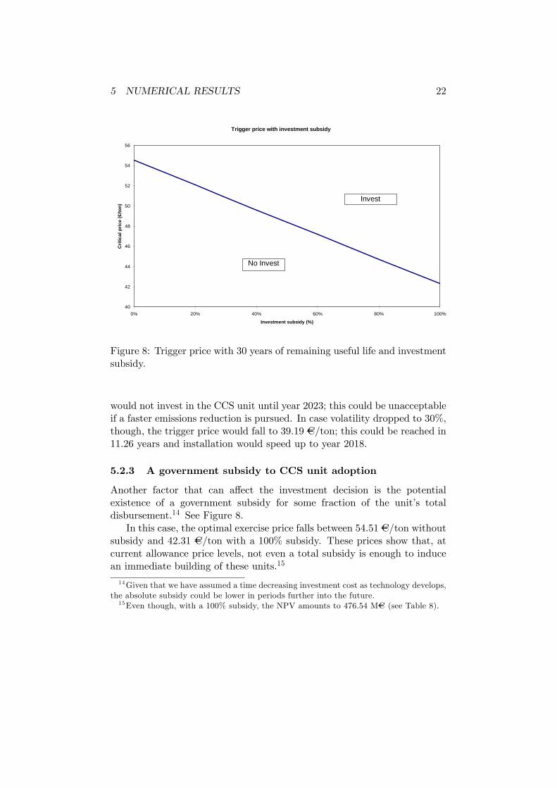
Another factor that can a¤ect the investment decision is the potentialexistence of a government subsidy for some fraction of the unit�s totaldisbursement.14 See Figure 8.

In this case, the optimal exercise price falls between 54.51 AC/ton withoutsubsidy and 42.31 AC/ton with a 100% subsidy. These prices show that, atcurrent allowance price levels, not even a total subsidy is enough to inducean immediate building of these units.15

14Given that we have assumed a time decreasing investment cost as technology develops,the absolute subsidy could be lower in periods further into the future.15Even though, with a 100% subsidy, the NPV amounts to 476.54 MAC (see Table 8).

6 CONCLUSIONS 23

6 Conclusions

In this paper we have analyzed the option to invest in a CCS unit usingstandard parameter values for it. Two correlated stochastic processes havebeen considered, one for the allowance price and the other one for electricityprice. Parameter values for these price processes have been calibrated fromthe European Trading Scheme (ETS) and the Spanish wholesale electricitymarket (OMEL).

Our results show that current permit prices do not provide an incentiveto the quick adoption of this technology, the more so when the option tochoose the optimal time to invest is considered. Immediate constructionby coal-�red power plants would be justi�ed for carbon prices close to 55AC/ton. This �gure is signi�cantly higher than 13.95 AC/ton which wouldresult from a simple NPV analysis. Plants with less than eight years ofremaining useful life would hardly adopt this technology at all, since therewould not be enough time to recover the investment. For all other termsof useful life, a carbon price close to 55 AC/ton is rather stable and almostindependent of the remaining life.

The high value of the trigger price is mainly driven by the high allowanceprice volatility (close to 47%). An structural market change bringing abouta sizeable drop in volatility would imply a signi�cant decrease in the optimalprice and, consequently, earlier adoption of this technology by utilities. Forexample, for a carbon price volatility of 20%, the trigger price falls to 32AC/ton.

We have also considered the possibility to promote these units by meansof a subsidy. When this is maximum (100 % of the unit�s initial cost),the optimal price approaches 42 AC/ton; this represents a drop of morethan 12 AC/ton from that without subsidy (or 22.38 %). All in all, thecurrent framework does not seem to encourage an early adoption of theCCS technology.

A better estimation of the stochastic model for the allowance price wouldbe feasible as long as we approach the second application phase of theKyoto Protocol (2008-2012), there are more futures prices for this periodand current uncertainties unfold (though new ones could appear).

The model may be applied to other types of power technologies, likenatural gas-�red combined cycle (NGCC) plants or integrated gasi�cationcombined cycle (IGCC) plants. In the �rst case, carbon emissions aresigni�cantly lower, 16 and in the second they are also lower but just becauseof the higher e¢ ciency of this facility.

The model can be extended in several ways. For instance, the possibilityto build a somewhat more expensive power plant but designed from theoutset to be "capture-ready"; that is, to disburse today a higher sum of

16About 350 g/kWh, depending on the plant�s e¢ ciency.

A APPENDIX 24

money in exchange for the option to incur less costs in the future should thecase for installing a CCS unit become compelling.

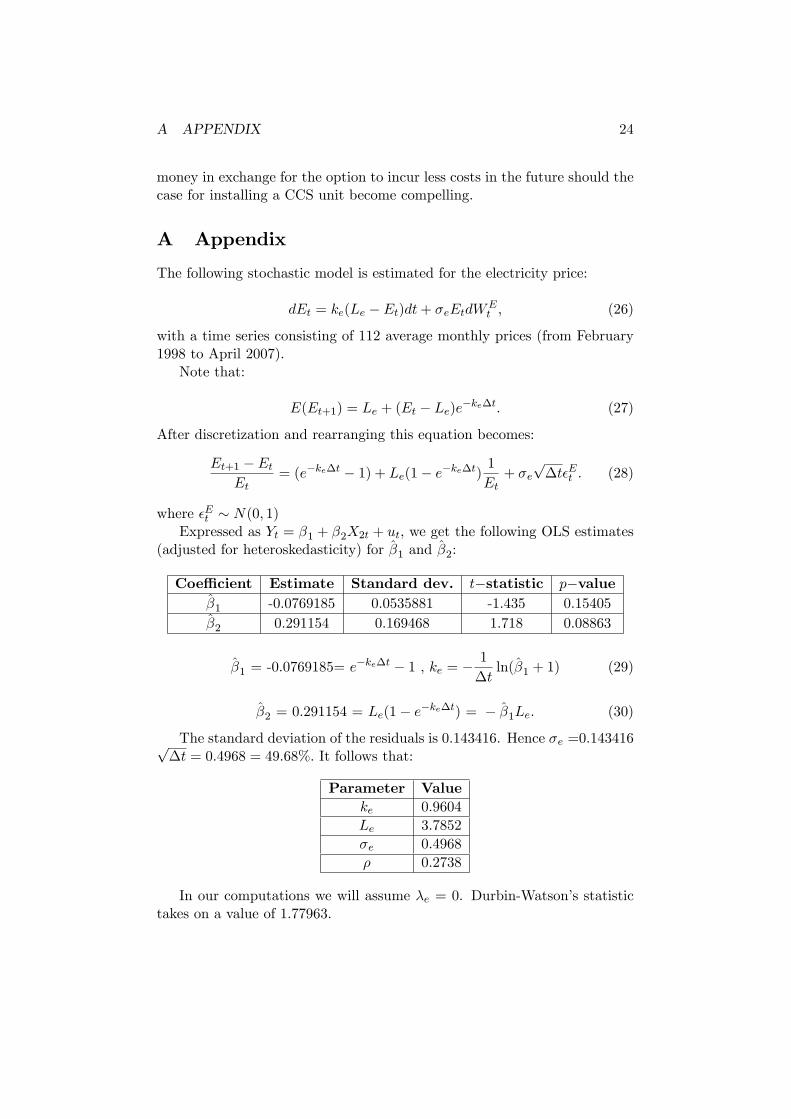
A Appendix

The following stochastic model is estimated for the electricity price:

dEt = ke(Le � Et)dt+ �eEtdWEt ; (26)

with a time series consisting of 112 average monthly prices (from February1998 to April 2007).

Note that:

E(Et+1) = Le + (Et � Le)e�ke�t: (27)

After discretization and rearranging this equation becomes:

Et+1 � EtEt

= (e�ke�t � 1) + Le(1� e�ke�t)1

Et+ �e

p�t�Et : (28)

where �Et � N(0; 1)Expressed as Yt = �1 + �2X2t + ut, we get the following OLS estimates

(adjusted for heteroskedasticity) for �1 and �2:

Coe¢ cient Estimate Standard dev. t�statistic p�value�1 -0.0769185 0.0535881 -1.435 0.15405�2 0.291154 0.169468 1.718 0.08863

�1 = -0.0769185= e�ke�t � 1 , ke = �

1

�tln(�1 + 1) (29)

�2 = 0.291154 = Le(1� e�ke�t) = � �1Le. (30)

The standard deviation of the residuals is 0.143416. Hence �e =0.143416p�t = 0:4968 = 49:68%: It follows that:

Parameter Valueke 0.9604Le 3.7852�e 0.4968� 0.2738

In our computations we will assume �e = 0. Durbin-Watson�s statistictakes on a value of 1.77963.

REFERENCES 25

References

[1] C. Böhringer, T. Ho¤man, A. Lange, A. Löschel and U. Moslener:"Assessing Emission Regulation in Europe: An Interactive SimulationApproach". The Energy Journal, Vol. 26, No. 4, pp. 1-21.

[2] M.J. Brennan and L. Trigeorgis: Project �exibility, agency, andcompetition. Oxford University Press, 2000.

[3] B. Buchner, C. Carraro and A.D. Ellerman: "The Allocation ofEuropean Union Allowances: Lessons, Unifying Themes and GeneralPrinciples". Fondazione Eni Enrico Mattei, Nota di Lavoro 116.2006,September 2006.

[4] P. Coombes, P. Graham and L. Reedman: "Using a Real-OptionsApproach to Model Technology Adoption Under Carbon PriceUncertainty: An Application to the Australian Electricity GenerationSector". The Economic Record, Vol. 82, Special Isssue, September 2006,pp. 64-73.

[5] A. K. Dixit and R. S. Pindyck: Investment under uncertainty. PrincetonUniversity Press, 1994.

[6] A.C. Harvey: Forecasting, structural time series models and theKalman �lter. Cambridge University Press, 1990.

[7] M. Insley: "On the Option to Invest in Pollution Control undera Regime of Tradable Emissions Allowances". Canadian Journal ofEconomics, Vol. 36, No. 4, pp. 860-883, 2003.

[8] H. Laurikka: "Option value of gasi�cation technology within anemission trading scheme". Energy Policy 34, 2006, pp. 3916-3928.

[9] H. Laurikka and T. Koljonen: "Emissions trading and investmentdecisions in the power sector: a case study in Findland". Energy Policy34, 2006, pp. 1063-1074.

[10] P. E. Kloeden and E. Platen �Numerical Solution of StochasticDi¤erential Equations�. Springer, 1992.

[11] S. Majd and R.S. Pindyck : "Time to build, option value, andinvestment decisions". Journal of Financial Economics 18: 7-27, 1987.

[12] J. Sarkis and M. Tamarkin: "Real Options Analysis for "GreenTrading": The Case of Greenhouse Gases". The EngineeringEconomist, 50, 273-294 (2005).

REFERENCES 26

[13] E. S. Schwartz �The Stochastic Behavior of Commodity Prices:Implications for Valuation and Hedging�The Journal of Finance, VolLII, No. 3, 923-973 (1997).

[14] E. S. Schwartz and L. Trigeorgis (eds): Real options and investmentunder uncertainty. The MIT Press, 2001.

[15] C. Sørensen �Modeling Seasonality in Agricultural CommodityFutures�. The Journal of Futures Market, Vol. 22, No. 5, 393-426 (2002).

[16] F. Teng and D. Tondeur: "E¢ ciency of carbon storage with leakage:phisical and economical approaches". Energy 32, 2007, pp. 540-548.

[17] L. Trigeorgis: Real options - Managerial �exibility and strategy inresource allocation. The MIT Press, 1996.

long-term dynamics in co allowance prices and carbon capture

Documents