hedonic prices of sulfur in coal under the u.s. so ... · hedonic prices of sulfur in coal under...

Hedonic Prices of Sulfur in Coal under the

U.S. SO2 Allowance Market

Toshi H. Arimura ∗

Sophia University

May 12, 2002

JEL Classification: Q2,Q28,Q41.

Key Words: Emissions; Marketable Permits, Hedonic Analysis, Coal Market

Abstract

This study investigates the efficiency of pollution permit markets by con-

ducting an empirical study of the U.S. SO2 market. A hedonic model of coal

price is estimated by using the coal price data from 1985 to 1998. The esti-

mation results showed that the sulfur premium was in the same order as the

SO2 allowance prices in the EPA auction. In addition, for 1997 and 1998, the

SO2 allowance prices were in 95% confidence intervals for a relevant range of

sulfur content levels. In 1995, however, the deviation of the SO2 allowance

price from the sulfur premium was found. This deviation may have been

caused by the market power of the coal mine companies in Montana and

Wyoming.

∗I am grateful to Professors Edward Foster and John Geweke for their advice. I wouldalso like to thank Professors Jay Coggins, Steve Polasky and Frances Homans for helpfulcomments. This research has been supported by the Japan Economic Research Foundationand Asahi Glass Foundation. Address: Department of Economics, Sophia University, 7-1Kioi-cho, Chiyoda-ku, Tokyo, 102-8554 Japan. E-mail: [email protected]

1

1 The Link between Coal Market and the

SO2 Allowance Market

The SO2 allowance market is a pollution permit market that the 1990 Clean

Air Act Amendments created to control sulfur dioxide (SO2) emissions from

electric utilities in the United States. There has been concern, however, that

the SO2 allowance market may not be reflecting the true marginal abatement

cost. There are a few reasons for this concern. First, the unexpected low

allowance price is considered to be evidence of a failure of the market. The

allowance price was expected to be around $500 before it started. But the

price dropped to about $ 60 in 1996. Second, Public Utility Commission

(PUC) regulation has been superimposed on the SO2 emission regulation. In

the literature, some analysts argue that this distorts decisions by power plant

managers and, hence, the SO2 market. Third, there is concern about the

auction mechanism run by the Environmental Protection Agency. Cason [5]

has shown that in theory the auction distorts bidders’ incentives; as a result,

the market price of the allowance will not be the true marginal abatement

cost.

In response to these concerns, Joskow et al. [9] studied the allowance

market and claimed that it is efficient. Coggins and Swinton [6], on the

other hand, estimated the marginal abatement cost at power plants in Wis-

consin and found that they are considerably higher than market prices for

allowances. These studies, however, do not directly answer the question of

the efficiency of the nation-wide SO2 allowance market.

Joskow et al. [9] showed that the market has developed well in a short

period by examining the transaction data of SO2 allowances. First, they com-

pared the allowance price from the EPA auction with the prices associated

with private confidential trades, reported from two brokers. The finding is

that those prices were almost identical by late 1994. Second, they examined

the EPA auction and found that almost none of privately offered allowances

were sold in the auctions in 1993 and 1994. In the auction, allowances from

the EPA’s special account are sold first. If there is more demand, privately

provided allowances are sold. In 1993 and 1994, however, very few privately

provided allowances were sold. Thus, the seller side auction bias played no

role in determining the allowance price. They also found that, as time goes

2

by, peculiar bidding prices have been disappearing, i.e., most bids have be-

come closer to the market prices. Finally, Joskow et al. investigated quantity

of the allowance trades and found that the quantity of allowance trades in

the EPA Auction has become a smaller part of the total private transactions.

For example, from April 1996 to March 1997, only 5.5 % of private allowance

trades took place in the auction. This fact implies that most allowance trans-

actions took place outside the EPA and that the number of transaction has

been increasing rapidly. From these observations, they concluded that the

allowance market “had become reasonably efficient.”

Coggins and Swinton [6] proposed an output distance function approach

to investigate the marginal abatement cost of SO2 emission at the plant level

in Wisconsin. On average, their estimate for the marginal abatement cost

was about $292.70 per ton of SO2 in constant 1992 dollars. Since the average

allowance price in the 1993 EPA auction was $156.00 per ton their results

showed a divergence between the allowance price and the marginal abatement

cost. They argued that the difference can be attributed to the stringent local

SO2 emission regulations in Wisconsin.

Other studies also found problems in the allowance market. Carlson et

al.[4] revealed that most trading gains were unrealized in the first two years of

the acid rain program. Arimura [1] investigated electric utility behavior under

the SO2 allowance market in Phase I. The study found that cost recovery

rules promoted high sulfur coal usage for utilities located in states with coal

mines. A comprehensive study of the SO2 allowance market by Ellerman et

al. [8] also pointed out imperfections of the allowance market. Swinton [10]

found that power plants in Florida can save abatement cost by participating

in the national market for allowances.

While these studies give useful information on how the SO2 allowance

market has been working, they do not answer the question of the SO2 al-

lowance market efficiency in view of economic theory. The efficiency of a

pollution permit market is determined by whether or not the marginal abate-

ment costs of polluters are equal to the price of a permit. This is the exact

reason why pollution permit markets are preferred to direct regulations. The

study of the SO2 allowance market by Joskow et al., however, did not ex-

amine whether allowance prices reflect the marginal abatement cost of SO2

emission. In order to estimate the marginal abatement cost, one should study

3

electric power utilities’s behavior such as fuel choices. What Joskow et al.

examined was the SO2 allowance transaction data, not utilities’ fuel choices

or investment in pollution abatement technology. While their study answered

many concerns about the allowance market, it did not reveal the relationship

between marginal abatement cost and the allowance price.

In contrast to Joskow et al., Coggins and Swinton [6] estimated the

marginal abatement cost at the power plant level. Their sample was, however,

taken only from Wisconsin while the allowance market is a nation-wide sys-

tem. Moreover, the sample covers only the years from 1990 to 1992, which

was three years before power utilities had to comply with the regulation.

Swinton [10] calculated the shadow price of emission reductions for power

plants using newer data set. However, the data is taken only from Florida.

Further, the output distance function approach in these studies does not have

a statistical theory as a basis. Thus, one cannot formally test to see if the

estimated marginal abatement costs are different from the allowance price.

No studies have directly investigated the link of the marginal abatement

cost and the allowance price. In the context of the SO2 allowance market,

electric utilities face choices between using SO2 allowances and using coal

with less sulfur content. If the sulfur content is smaller, the SO2 emission

is smaller; therefore, they can save the cost of the SO2 allowance. Thus,

theoretically, the sulfur premium should be reflected in the SO2 allowance

market. Thus, one solution to this question is to investigate the coal market

by examining sulfur premiums in coal prices. In this paper, the sulfur pre-

mium is defined as an additional cost that power plant managers have to pay

in order to purchase coal with less sulfur content. By statistically analyzing

this premium from a coal transaction data set, one can investigate whether

or not the SO2 allowance market reflects the true marginal abatement cost.

2 Data

All the transactions of fossil fuels at power plants are reported to the Energy

Information Administration (EIA) and are kept as EIA423. I have obtained

the data for the period of 1985-1998 from EIA. The data contain coal prices,

sulfur content, ash content, heat content (mmBtu), quantity, month, year

and plant code.

4

The EIA423 data set includes contract type for each purchase as well.

Table 1 compares the number of spot purchases and total purchases in the

years of 1985 and 1995. How coal prices are determined in contract is a

dynamic decision. Therefore, the econometric study below focuses on coal

prices in the spot market.

Table 1: Number of Transactions by Contract Type

Number of Coal Transaction in Each Year

Contract Type 1985 1995

Spot Purchase 7773 7970

Total Purchase 19605 20222

The EIA423 contains coal type that has five categories: bituminous, sub-

bituminous, anthracite, lignite and bitumen. Table 2 reports the number

of purchases for each coal type in 1985 and 1995. Bituminous and sub-

bituminous accounts for 95 % of coal purchase in both years. Sub-bituminous

coal purchases have almost doubled in ten years while purchases of bitumi-

nous coal decreased. This is consistent with the literature ([3] and [7]).

Table 2: Number of Transactions by Coal Type

Both

(Spot & Contract) Spot

Coal Type 1985 1995 1985 1995

Bituminous 17733 16798 7166 6646

Sub-Bituminous 1416 2827 170 770

Lignite Coal 223 272 1 0

Anthracite Coal 176 86 101 34

5

3 Model

3.1 Theoretical Model

This study focuses on spot purchases since contract purchase is a complex

dynamic decision. Given capacity sizes, plant managers face K types of coal

and choose coal purchase qk, measured in heat, for each type (k = 1, ·, K).

Sulfur content for each type of coal is denoted by sk. The SO2 emission from

the plant at time t is given as:

Et ≡ cK∑

k=1

skqk (1)

where c is a conversion unit from sulfur to sulfur dioxides.

Each coal type differs in other characteristics such as weight per heat

(wk) or ash content (ak). In this section, Xk is used to refer to k type coal

characteristics where Xk = ak, wh, ... Coal type is also included in Xk. Thus,

the production technology is assumed as follows:

y = f(∑

qk,∑

qkXk) (2)

where y is an exogenously given output level. According to an EPA report

[11], the production technology is not a function of sulfur content. Thus, it

is assumed that sulfur content does not enter the production function as an

element while the sulfur content affects SO2 emissions.

Let pkt and pa

t denote the price of coal type k and the allowance price at

time t, respectively. Then, the plant manager’s problem is to choose quantity

of coal purchase for each level of sulfur, q(s), such that

minqkk

K∑

k=1

pkt q

k + pat Et (3)

subject to (2).

Plugging (1) into (3), the problem is equivalent to the following:

minqkk

K∑

k=1

pkqk + pat

K∑k=1

skqk (4)

6

subject to (2).

Claim: Coal price pk is a linear function of sulfur content under the SO2

allowance market.

Proof: The Lagrangian for the cost minimization problem is given as:

L = K∑

k=1

pkqk + pat

K∑k=1

skqk

+λy − f(∑

qk,∑

qkXk). (5)

Thus, the first order condition for a purchase coal qk > 0 is

∂L/∂qk = pk + pat s

k − λf1 +∑

1,·,Mfm+1(

∑qk,

∑qkXk)Xk

m = 0. (6)

where fm is the first derivative of the production function with respect to

element no. m. Thus, if coal type k is purchased, the price in an equilibrium

is given as follows:

pk = −pat s

k + λf1 +∑

1,·,Mfm+1(

∑qk,

∑qkXk)Xk

m. (7)

This proves that the coal price is linear in sulfur content under the SO2

allowance market.

To understand the model, let us look at Figure 6, which shows relation-

ships between coal prices and sulfur contents of coal purchase for two different

plants. The manager of plant A faces various coal prices denoted by ‘∗’ and‘x’. Among all the possibility, the manager is willing to purchase the lowest

price coal including SO2 emission cost. The slope of solid line is given by the

allowance price. Consequently, the manager chooses to purchase the coal on

the plain line, which is denoted by ‘∗’.If the plant is in a different location, the manger faces different potential

coal prices as shown in the Figure as Plant B. In this case, Plant B is

located more distant from coal mines. This is captured by the intercepts,

which are different across plants. As a result, the managers pays more for

coal. However, the sulfur premium given by the slope of the brake line should

7

be the same with Plant A because the allowance price is the same for both

managers. The price of purchased coal are denoted by ‘o’; the un-purchased

coal is given by ‘.’.

The model assumes that plant managers are price takers and they have

no influence on coal prices. This point may need to be taken care of when

estimation results are discussed.

3.2 Econometric Model

The following model is examined:

Pitj = β1 +1998∑

year=1985

θ1,yearsijt + θ2,year(sitj)2 + θ3,year(sitj)

3Dyear,ijt

+β2aitj + Σβcoaltype3 Dcoaltype

itj + β4BTUitj + uitj (8)

where i, t and j denote plant, time (month) and j th purchase of coal at

plant i at time t, respectively. Dummy variable Dyear,ijt is used to capture

sulfur premium year by year. Price of j th coal at plant i and at time t (cents

per mmBtus) is Pitj . Sulfur content, sitj, and ash content, aitj, are measured

in pounds per mmBtu. BTUitj captures heat content measured in btu per

pound.

Dummy variables for each coal type are Dcoaltypeitj where there are five

categories as stated in the preceding section: bituminous, sub-bituminous,

lignite, anthracite and bitumen. Parameters to be estimated are θm,yearyaer

(m=1,2,3) and β. The term uitj is to capture unobservable part of the cost

structure.

The coefficient of sulfur content, θ1,year, is expected to be negative if the

sulfur premium is captured by coal prices. Once the allowance market started

(year ≥ 1995), the size of θ1,year should be equal to the allowance price for

each year. Moreover, if the model in the previous section holds, it must hold

that θ2,year = θ3,year = 0 after the year of 1995.

The coefficient of ash, β2, is expected to be negative since ash requires

some treatment in combustion. The sign of β4 is expected to be positive

since the larger heat content implies less cost per heat for moving the coal in

plant.

8

4 Specifications

4.1 Tests for the Specifications

In order to implement statistical tests on estimated parameters, the variance

covariance structure of error terms in (8) must be correctly specified. Several

specification tests are conducted to capture error structures. However, im-

plementing these tests are difficult for unbalanced data sets. Therefore, using

the original data set, a balanced panel data set is constructed by selecting

observations of plants that have coal purchase information for all the months

in 1995. Thus,

pit = Xitβ + uit (9)

where i = 1, ..., N and t = 1, ...., T . For the balanced data set, N = 92 and

T = 12. The regressors are

Xit = 1, sit, s2it, s

3it, ait, D

SUBit , BTUit. (10)

First, it is tested whether there is an individual effect at the plant. Thus,

the following error structure is examined:

uit = µi + νit (11)

where µi and νit are normally distributed with variance σ2µ and σ2

ν respec-

tively. The test is conducted to examine

Ho : σµ = 0

versus

Ha : σµ = 0.

Breush and Pagan [2] showed that the Lagrangian Multiplier statistics for

the test is given by:

LM =NT

2(T − 1)[u′(IN

⊗eTe

′T )u

u′u− 1]2 (12)

where the statistic is distributed as χ2(1) under the null hypothesis.

Using the balanced panel data set, the test statistic is found to be 10.928.

Thus, the null hypothesis is rejected at the 1.0 % level.

9

Next, the Hausman test is conducted to examine orthogonality of the

random effects. Namely, the hypothesis are:

Ho : E[µi|X] = 0

versus

Ha : E[µi|X] = 0.

Under the null, the test statistic is distributed as χ2 with 6 degrees of freedom.

For the panel data set, the statistic is 6.5054. The null hypothesis is not

rejected at the 1 % significance level. This provides evidence in favor of a

random effect model over a fixed effect model. Therefore, the random effect

model is examined in the following.

Finally, the time component of the error is tested. The following error

structure is considered:

uit = λt + νit (13)

where λt and νit are normally distributed with variance σ2λ and σ2

ν respec-

tively. The test is conducted to examine

Ho : σλ = 0

versus

Ha : σλ = 0.

Breush and Pagan [2] showed that the Lagrangian Multiplier statistics for

the test is given by:

LM =NT

2(N − 1)[u′(eNe′N

⊗IT )u

u′u− 1]2 (14)

where LM is distributed as χ2(1) under the null hypothesis. Since the value

of the test statistic is 554.36, the null hypothesis is rejected at the 1% level.

4.2 Error Specifications

The specification tests above reveals that the model to be examined is given

as follows:

pitj = Xitjβ + uitj (15)

10

where

Xitj = sitj, s2itj, s

3itj, aitj, D

SUBitj , DBIT

itj , BTUitj. (16)

and

uitj = µi + λt + νitj . (17)

Estimating this model by GLS is not straightforward since the original

data is an unbalanced panel. On the other hand, many observations are lost

if the balanced panel is used. One can eliminate individual effect and time

effect by taking the first difference of (15). The first difference equation is

given as follows:

pitj+1 − pitj = Xitj+1β + uitj+1 − Xitjβ + uitj= (Xitj+1 −Xitj)β + νitj+1 − νitj (18)

when the plant identification number and purchased month for itj and

itj + 1 are equal. Under this first difference model, the sample size for

1995 is 5232. Thus, this estimation method provides a much larger sample.

Let us reparametrize the error term of the first difference equation as

εitj = νitj+1 − νitj. Then, E[εε′] = σ2νΩ where the diagonal element of Ω is

2 and where the first off-diagonal element is −1 for each plant in the same

month. The rest of elements of Ω are zero. Even though this is a relatively

simple variance-covariance matrix, the estimation is not straightforward since

the panel data is unbalanced and since the sample size is large.

5 Results and Discussion

5.1 OLS Results with the First Difference Equation

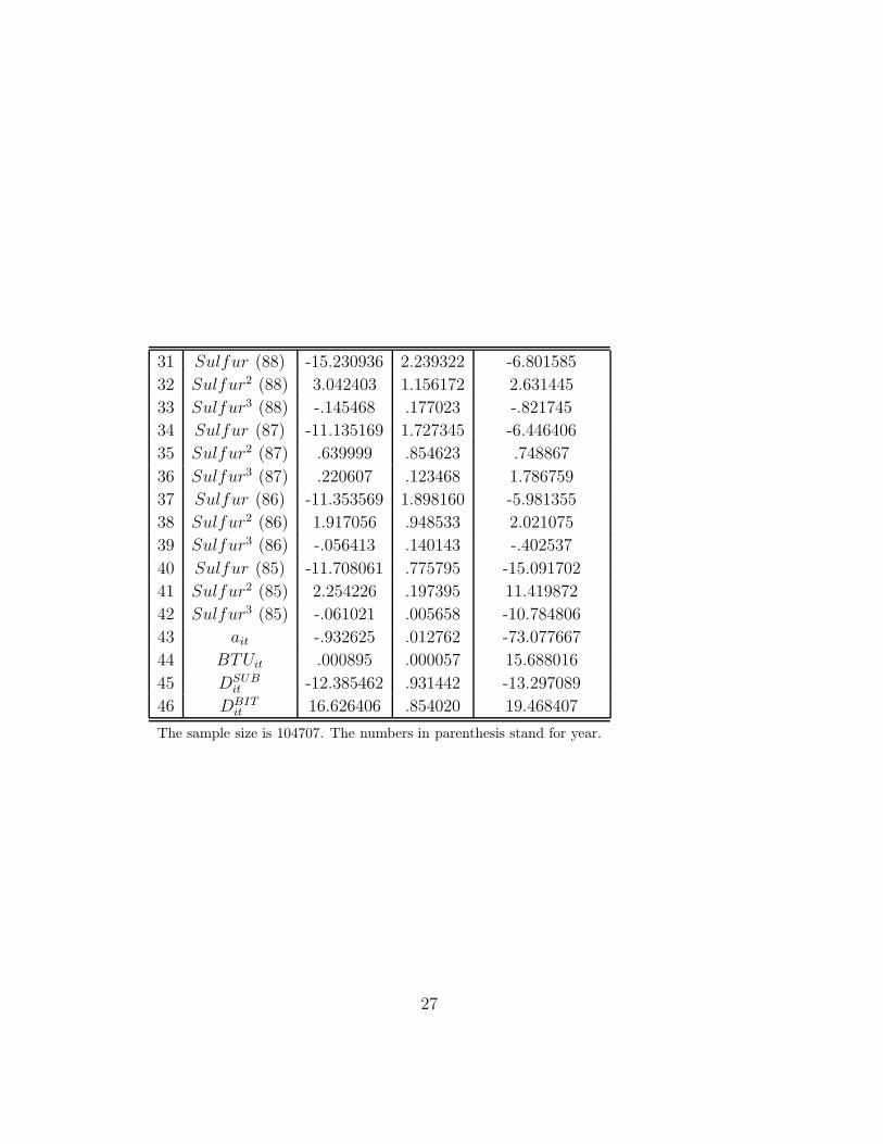
The OLS estimation is conducted using equation (18). The sample consists of

the observations from 1985 to 1998 and the size is 138808. After taking first

differences, the sample size for the estimation is 104707. The OLS estimates

are consistent even though hypothesis testing cannot be conducted without

the correction of the variance covariance matrix. The estimation results are

reported in Table 6 in Appendix. The standard errors are computed using

the correct variance-covariance structure. In a later section, using dummy

11

variables for states of origin of coal is discussed to capture some unobservable

coal characteristics. The regression results for this case are also reported in

the Appendix.

5.2 Sulfur Premium

Once the parameters are estimated in the linear model (8), one can derive

the sulfur premium (−∂Pitj/∂sitj) in the coal market as follows:

SulfurPremium = −θ1,year + 2θ2,year(sitj) + 3θ3,year(sitj)2 (19)

where Pitj is the coal price measured in cents, sitj is the sulfur content mea-

sured in pounds per mmBtu, and θ1,year, θ2,year, θ3,year are the estimated

parameters. Thus, the sulfur premium can be computed as a function of the

sulfur content. If the theory holds, one expects the sulfur premium to be

approximately equal to the SO2 allowance price for all sulfur content levels

once the allowance market started (θ2 = θ3 = 0). On the other hand, before

the allowance market was introduced in 1995, sulfur premiums do not have

to be constant for the whole sulfur content range since plant managers did

not have to hold SO2 allowances.

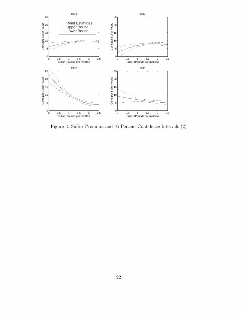
The 95 percent confidence intervals for the sulfur premium are computed

for each year. The results are shown in Fig. 6, 6, 6 and 6. In order to

investigate the relation between the allowance market and the coal market,

let us examine the allowance price. In the EPA auction, the allowance was

$130 per ton in 1995. With units converted, the price is equivalent to 13

centss per SO2 kg, which is equivalent to about 14 cents per sulfur pound.

The allowance prices from the spot market are shown in the dotted lines for

each year after the allowance market had started. The sulfur premium and

allowance prices are in the same order even though the allowance prices from

the EPA auction are not necessarily in the 95% confidence interval of sulfur

premium. The coal market seems to reflect the allowance price as the sulfur

premium.

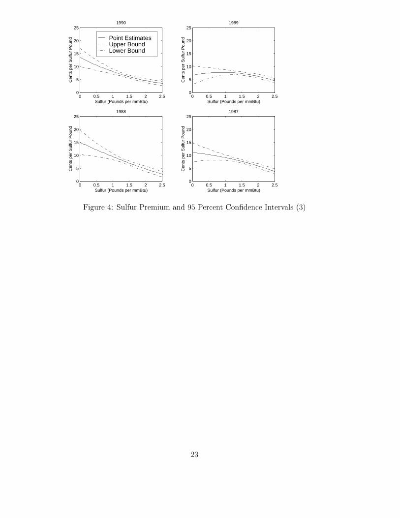
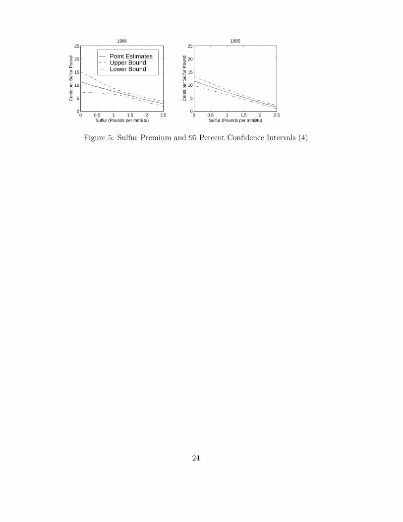
Figure 3, 4 and 5 show that positive sulfur premium was found even

before he SO2 allowance market was introduced. This is an expected result

since coal power plants were often subject to various local SO2 regulations.

To deal with local air pollition problems, EPA enforced local governments to

12

take policies toward SO2 emission contorls. In many cases, local regulatory

authourities put some restrictions on coal type usage, meaured by sulfur or

sulfur dioxide per mmBtu. Although these regulations were not as tight

as the acid rain program requirements, this is considered to cause sulfur

premium before the SO2 allowance market.

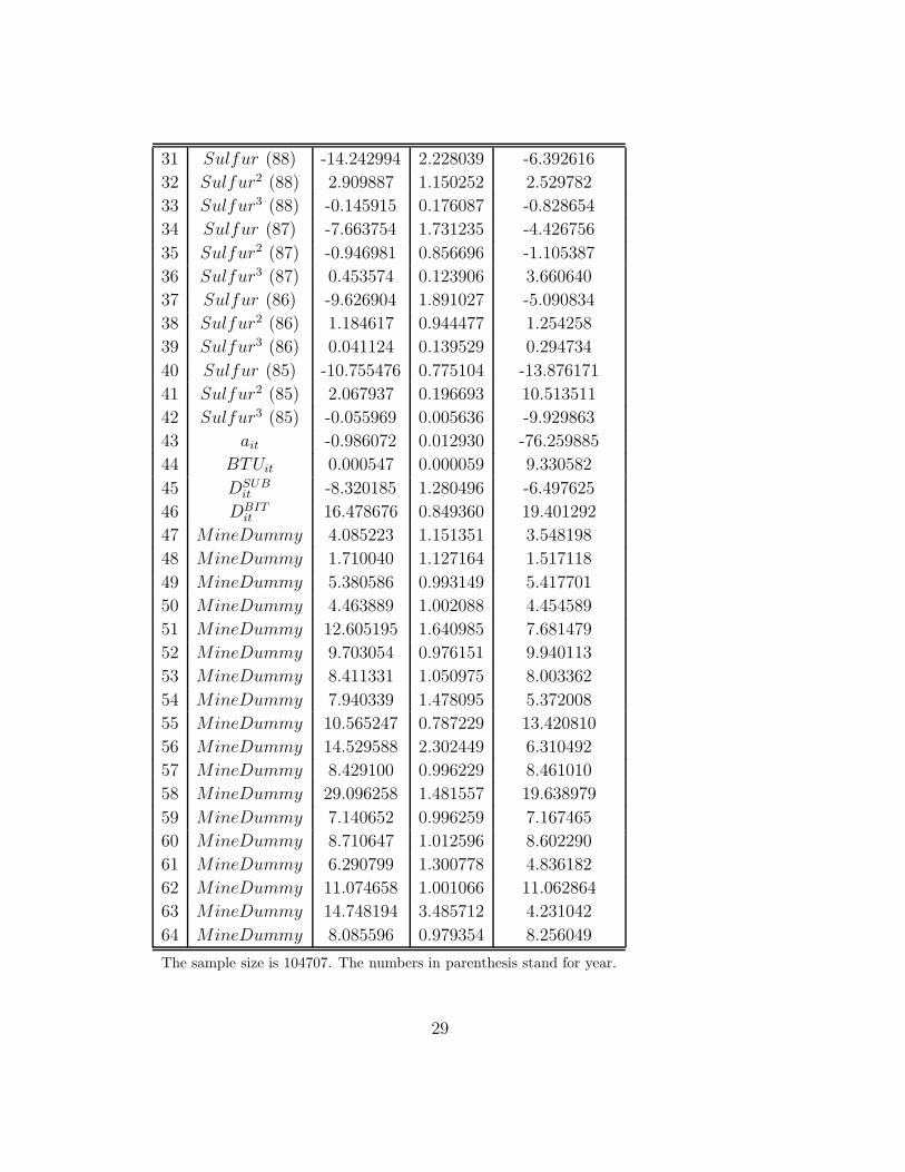
5.3 Issue of Choice of Regressors

Unobservable coal characteristics such as moisture content or volatility may

affect the efficiency of electricity generation. These characteristics can be

considered to depend on the location of coal mines. There are 16 states

with coal mines in the sample. In order to capture these effects, dummy

variables DMineStateitj t are constructed to refers to each state where the coal

is from. The random effect model is not considered due to complication

from the unbalanced panel.The OLS results with the dummy DMineStateitj

are reported in the Appendix. The estimates do not seem to change to a

great degree in spite of the addition of the dummy variables.

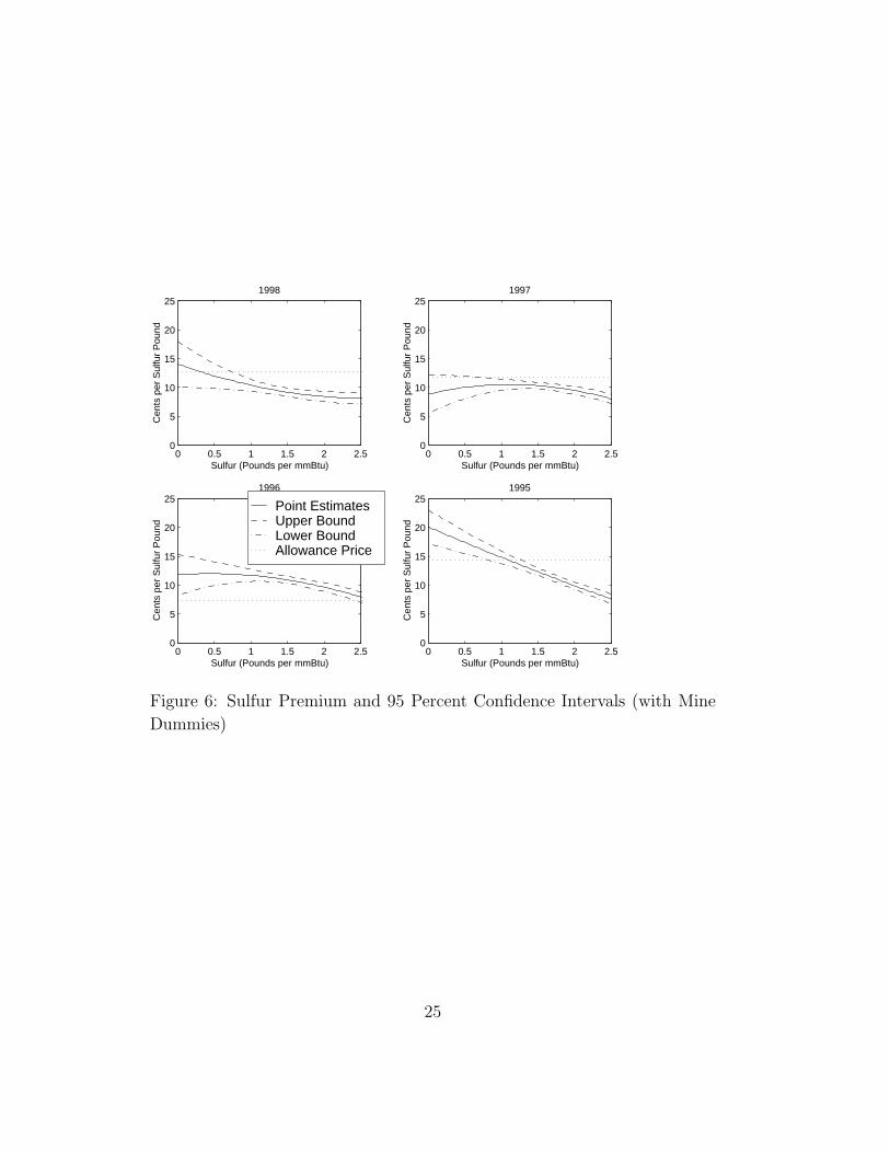
Using these estimates, 95 percent confidence intervals for the sulfur pre-

mium are computed for each year. The results are shown in Appendix (Fig.

6). Fig. 6 presents the 95 % confidence intervals of sulfur premium after the

SO2 regulation of the acid rain program started. The allowance price in EPA

auction for each year is drawn by dot lines. For 1997 and 1998, the allowance

price is in the range of 95% confidence intervals for sulfur premium from 0 to

1 pound per mmBtu. This suggests that the allowance prices in the auction

reflect the sulfur premium of coal for low sulfur coal.

In 1995, the sulfur preimum was higher for lower sulfur coal. Specifically,

the premium was hihger than the allowance price in the EPA auction for

the range of sulfur from 0 to 0.6 pound. This suggests that plant mangers

paid more than necessary high price for the lower sulfur coal within that

range. Most subbituminous coal from the West are in that range. Therefore,

this result may provide evidence that coal mine company in the West took

advantage of the introduction of the SO2 market by exploiting rent from the

higher coal price.

13

5.4 Linear Hypothesis Testing

The cost minimizing model in a previous section implies that sulfur premium

is linear in sulfur content. Wald tests are conducted in order to test this

linear hypotheses (θ2 = θ3 = 0) for each year. Test statistic are computed for

both estimations: 1) regression with Eq. (8) and 2) regression with dummy

variables for states of mine data. The statistics are reported in Table 3.

Under the null hypotheses, the test statistics has a chi-squared distribu-

tion with 2 degrees of freedom. The critical value of the chi-squared distri-

bution is 9.21 at the 1 % significance level. Therefore, the hypotheses are

not rejected for 1998 and 1991 in both estimations. However, the hypothesis

are rejected for other years.

5.5 Discussion

The statistical analysis in the previous subsections showed that the allowance

price did not reflect marginal abatement cost in the first two years. How-

ever, in 1997 and 1998, for lower range of sulfur content, coal price reflected

allowance prices. Further, the linear hypothesis, which is expected to hold

in the market, was accepted in 1998.

These results are consistet with Carlson et al.[4]. They found that the

advantage of pollution-permit market was not realized in the first two years.

The analysis in the previous sections provide evidence from another aspect:

the deviation between sulfur premium in the coal and the allowance price.

However, the analysis above found that the market is becoming efficient

in 1997 and 1998 in the sense that the deviation vanished for lower range

of sulfur coal. This is an supporting evidence that the market “had become

reasonably efficient(Joskow et al.[9]).”

6 Conclusion

In this study, the efficiency of the U.S. SO2 allowance market was examined.

Specifically, hedonic analysis was conducted in order to find the link between

14

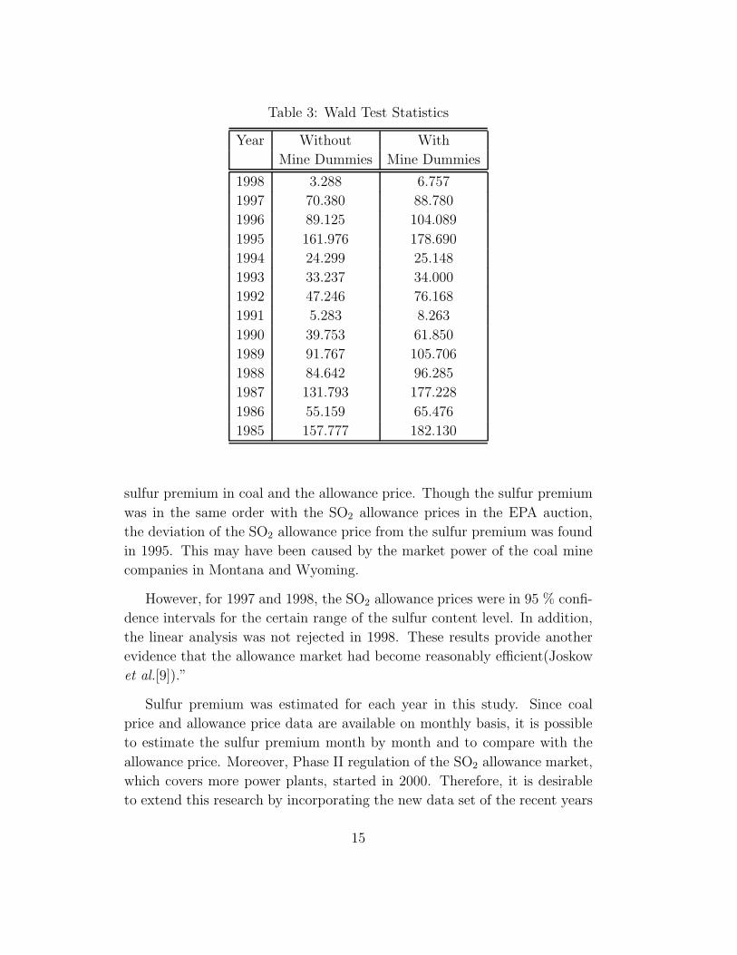
Table 3: Wald Test Statistics

Year Without With

Mine Dummies Mine Dummies

1998 3.288 6.757

1997 70.380 88.780

1996 89.125 104.089

1995 161.976 178.690

1994 24.299 25.148

1993 33.237 34.000

1992 47.246 76.168

1991 5.283 8.263

1990 39.753 61.850

1989 91.767 105.706

1988 84.642 96.285

1987 131.793 177.228

1986 55.159 65.476

1985 157.777 182.130

sulfur premium in coal and the allowance price. Though the sulfur premium

was in the same order with the SO2 allowance prices in the EPA auction,

the deviation of the SO2 allowance price from the sulfur premium was found

in 1995. This may have been caused by the market power of the coal mine

companies in Montana and Wyoming.

However, for 1997 and 1998, the SO2 allowance prices were in 95 % confi-

dence intervals for the certain range of the sulfur content level. In addition,

the linear analysis was not rejected in 1998. These results provide another

evidence that the allowance market had become reasonably efficient(Joskow

et al.[9]).”

Sulfur premium was estimated for each year in this study. Since coal

price and allowance price data are available on monthly basis, it is possible

to estimate the sulfur premium month by month and to compare with the

allowance price. Moreover, Phase II regulation of the SO2 allowance market,

which covers more power plants, started in 2000. Therefore, it is desirable

to extend this research by incorporating the new data set of the recent years

15

including Phase II period. These are areas of future work.

16

References

[1] T. H. Arimura. An empirical study of the SO2 allowance market: Ef-

fects of PUC regulations. forthcoming in. Journal of Environmental

Economics and Management.

[2] T Brusch and A. Pagan. The LM test and its applications to model

specification in econometrics. Review of Economics and Studies, 47:239–

254, 1980.

[3] D. Burtraw. Cost savings sans allowance trades? Evaluating the SO2

emission trading program to date. Contemporary Economic Policy,

14:.79–94, 1996.

[4] C. Carlson, D. Burtraw, M. Copper, and K. L. Palmer. Sulfur dioxide

control by electric utilities: What are the gains from trade. Journal of

Political Economy, 108, 2000.

[5] T. N. Cason. Seller incentive properties of epa’s emission trading auc-

tion. Journal of Environmental Economics and Management, 25(2):177–

95, 1993.

[6] J. S. Coggins and J. R. Swinton. The price of pollution: A dual approach

to valuing SO2 allowances. Journal of Environmental Economics and

Management, 30:58–72, 1996.

[7] A. D. Ellerman and J. Montero. The declining trend in sulfur dioxide

emissions: Implications for allowance prices. Journal of Environmental

Economics and Management, 36:26–45, 1998.

[8] A.D. Ellerman, P. L. Joskow, R. Schmalensee, J. P .Montero, and E.M.

Bailey. Markets for Clean Air: the U.S. Acid Rain Program. Cambridge

University Press, Cambridge, United Kingdom, 2000.

[9] P. L. Joskow, R. Schmalensee, and E. M. Bailey. The market for sulfur

dioxide emissions. American Economic Review, 88:669–685, 1998.

[10] J. R. Swinton. The potential for cost savings in the SO2 allowance mar-

ket: Empirical evidence from florida, forthcoming in. Land Economics,

2002.

17

[11] US Energy Information Administration. Acid Rain Compliance Strate-

gies for the Clean Air Act Amendments of 1990. Washington DC, 1994.

18

Appendix

Table 4: Descriptive Statistics for Fuel 1985 Coal Spot Purchase

Variables Means Std.Dev. Max Min

Price 142.1035 29.5968 399.000 21.900

D10 0.0922 0.2893 1.000 0.000

D11 0.0914 0.2882 1.000 0.000

D12 0.0948 0.2929 1.000 0.000

Sulfur 1.3880 0.8439 6.214 0.017

Sulfur2 2.6387 3.3617 38.614 0.000

Sulfur3 6.3862 12.8713 239.946 0.000

Ash 9.3424 4.9132 62.139 0.142

Surface 0.7155 0.4512 1.000 0.000

BIT 0.9509 0.2160 1.000 0.000

SUB 0.0220 0.1467 1.000 0.000

ANT 0.0210 0.1433 1.000 0.000

LIG 0.0009 0.0300 1.000 0.000

The sample size is 7767

19

Table 5: Descriptive Statistics for Fuel 1995 Coal Spot Purchase

Variables Means Std.Dev. Max Min

Price 118.2756 27.4035 224.100 0.100

Sulfur 1.2216 0.8883 8.411 0.024

Sulfur2 2.2812 3.5984 70.745 0.001

Sulfur3 5.8058 15.6039 595.036 0.000

Ash 9.7844 19.8779 1032.218 0.064

quantity 20065.2593 33661.0046 484000.000 10.000

Surface 0.5909 0.4917 1.000 0.000

BIT 0.8644 0.3424 1.000 0.000

SUB 0.1014 0.3018 1.000 0.000

ANT 0.0108 0.1034 1.000 0.000

The sample size is 7951

0 1 2 3 4 5 650

100

150

200

250

300Coal Prices in Different Plants

Cen

ts p

er S

ulfu

r P

ound

Sulfur (Pounds per mmBtu)

Plant APlant B

Figure 1: Illustration

20

0 0.5 1 1.5 2 2.50

5

10

15

20

25 1998

Cen

ts p

er S

ulfu

r P

ound

Sulfur (Pounds per mmBtu)0 0.5 1 1.5 2 2.5

0

5

10

15

20

25 1997

Cen

ts p

er S

ulfu

r P

ound


0 0.5 1 1.5 2 2.50

5

10

15

20

25 1996

Cen

ts p

er S

ulfu

r P

ound


Point EstimatesUpper BoundLower BoundAllowance Price

0 0.5 1 1.5 2 2.50

5

10

15

20

25 1995

Cen

ts p

er S

ulfu

r P

ound


Figure 2: Sulfur Premium and 95 Percent Confidence Intervals(1)

21

0 0.5 1 1.5 2 2.50

5

10

15

20

25 1994

Cen

ts p

er S

ulfu

r P

ound


Point EstimatesUpper BoundLower Bound

0 0.5 1 1.5 2 2.50

5

10

15

20

25 1993

Cen

ts p

er S

ulfu

r P

ound


0 0.5 1 1.5 2 2.50

5

10

15

20

25 1992

Cen

ts p

er S

ulfu

r P

ound


0

5

10

15

20

25 1991

Cen

ts p

er S

ulfu

r P

ound


Figure 3: Sulfur Premium and 95 Percent Confidence Intervals (2)

22

0 0.5 1 1.5 2 2.50

5

10

15

20

25 1990

Cen

ts p

er S

ulfu

r P

ound



0 0.5 1 1.5 2 2.50

5

10

15

20

25 1989

Cen

ts p

er S

ulfu

r P

ound


0 0.5 1 1.5 2 2.50

5

10

15

20

25 1988

Cen

ts p

er S

ulfu

r P

ound


0

5

10

15

20

25 1987

Cen

ts p

er S

ulfu

r P

ound



23

0 0.5 1 1.5 2 2.50

5

10

15

20

25 1986

Cen

ts p

er S

ulfu

r P

ound



0 0.5 1 1.5 2 2.50

5

10

15

20

25 1985

Cen

ts p

er S

ulfu

r P

ound



24

0 0.5 1 1.5 2 2.50

5

10

15

20

25 1998

Cen

ts p

er S

ulfu

r P

ound


0

5

10

15

20

25 1997

Cen

ts p

er S

ulfu

r P

ound


0 0.5 1 1.5 2 2.50

5

10

15

20

25 1996

Cen

ts p

er S

ulfu

r P

ound


Point EstimatesUpper BoundLower BoundAllowance Price

0 0.5 1 1.5 2 2.50

5

10

15

20

25 1995

Cen

ts p

er S

ulfu

r P

ound


Figure 6: Sulfur Premium and 95 Percent Confidence Intervals (with Mine

Dummies)

25

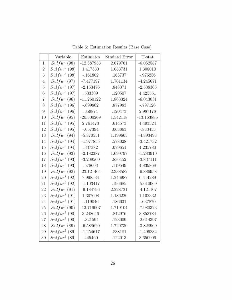
Table 6: Estimation Results (Base Case)

Variable Estimates Stndard Error T-stat

1 Sulfur (98) -12.587933 2.079761 -6.052587

2 Sulfur2 (98) 1.417530 1.083731 1.308010

3 Sulfur3 (98) -.161802 .165737 -.976256

4 Sulfur (97) -7.477197 1.761134 -4.245671

5 Sulfur2 (97) -2.153476 .848371 -2.538365

6 Sulfur3 (97) .533309 .120507 4.425551

7 Sulfur (96) -11.260122 1.863324 -6.043031

8 Sulfur2 (96) -.699862 .877983 -.797126

9 Sulfur3 (96) .359874 .120473 2.987178

10 Sulfur (95) -20.300269 1.542118 -13.163885

11 Sulfur2 (95) 2.761473 .614573 4.493324

12 Sulfur3 (95) -.057394 .068863 -.833453

13 Sulfur (94) -5.870551 1.199665 -4.893493

14 Sulfur2 (94) -1.977855 .578028 -3.421732

15 Sulfur3 (94) .337382 .079651 4.235780

16 Sulfur (93) -2.182387 1.699797 -1.283910

17 Sulfur2 (93) -3.209560 .836452 -3.837111

18 Sulfur3 (93) .578603 .119549 4.839868

19 Sulfur (92) -23.121464 2.338582 -9.886958

20 Sulfur2 (92) 7.998534 1.246987 6.414289

21 Sulfur3 (92) -1.103417 .196685 -5.610069

22 Sulfur (91) -9.184796 2.228721 -4.121107

23 Sulfur2 (91) 1.307608 1.186220 1.102332

24 Sulfur3 (91) -.119046 .186631 -.637870

25 Sulfur (90) -13.719007 1.719104 -7.980323

26 Sulfur2 (90) 3.248646 .842976 3.853784

27 Sulfur3 (90) -.321594 .123009 -2.614397

28 Sulfur (89) -6.588620 1.720730 -3.828969

29 Sulfur2 (89) -1.254617 .838181 -1.496834

30 Sulfur3 (89) .445460 .122013 3.650906

26

31 Sulfur (88) -15.230936 2.239322 -6.801585

32 Sulfur2 (88) 3.042403 1.156172 2.631445

33 Sulfur3 (88) -.145468 .177023 -.821745

34 Sulfur (87) -11.135169 1.727345 -6.446406

35 Sulfur2 (87) .639999 .854623 .748867

36 Sulfur3 (87) .220607 .123468 1.786759

37 Sulfur (86) -11.353569 1.898160 -5.981355

38 Sulfur2 (86) 1.917056 .948533 2.021075

39 Sulfur3 (86) -.056413 .140143 -.402537

40 Sulfur (85) -11.708061 .775795 -15.091702

41 Sulfur2 (85) 2.254226 .197395 11.419872

42 Sulfur3 (85) -.061021 .005658 -10.784806

43 ait -.932625 .012762 -73.077667

44 BTUit .000895 .000057 15.688016

45 DSUBit -12.385462 .931442 -13.297089

46 DBITit 16.626406 .854020 19.468407

The sample size is 104707. The numbers in parenthesis stand for year.

27

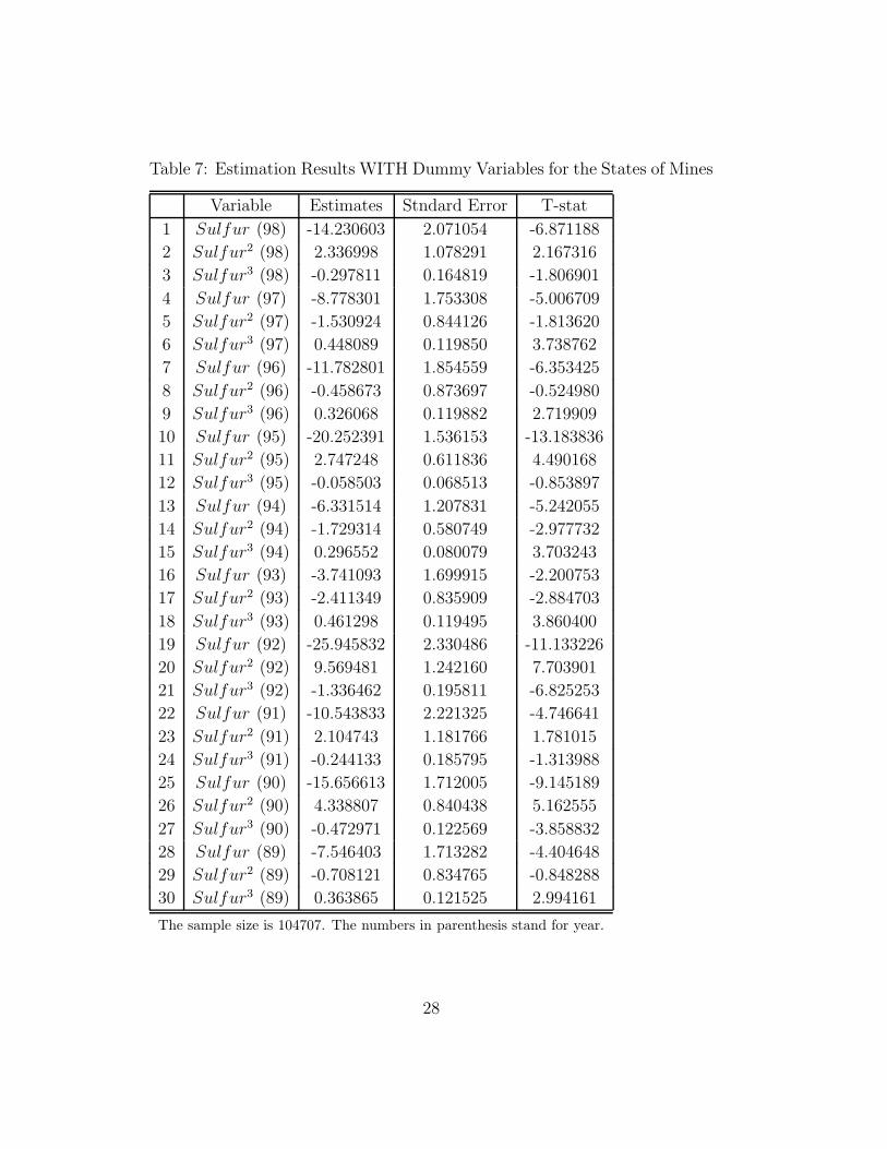
Table 7: Estimation Results WITH Dummy Variables for the States of Mines

Variable Estimates Stndard Error T-stat

1 Sulfur (98) -14.230603 2.071054 -6.871188

2 Sulfur2 (98) 2.336998 1.078291 2.167316

3 Sulfur3 (98) -0.297811 0.164819 -1.806901

4 Sulfur (97) -8.778301 1.753308 -5.006709

5 Sulfur2 (97) -1.530924 0.844126 -1.813620

6 Sulfur3 (97) 0.448089 0.119850 3.738762

7 Sulfur (96) -11.782801 1.854559 -6.353425

8 Sulfur2 (96) -0.458673 0.873697 -0.524980

9 Sulfur3 (96) 0.326068 0.119882 2.719909

10 Sulfur (95) -20.252391 1.536153 -13.183836

11 Sulfur2 (95) 2.747248 0.611836 4.490168

12 Sulfur3 (95) -0.058503 0.068513 -0.853897

13 Sulfur (94) -6.331514 1.207831 -5.242055

14 Sulfur2 (94) -1.729314 0.580749 -2.977732

15 Sulfur3 (94) 0.296552 0.080079 3.703243

16 Sulfur (93) -3.741093 1.699915 -2.200753

17 Sulfur2 (93) -2.411349 0.835909 -2.884703

18 Sulfur3 (93) 0.461298 0.119495 3.860400

19 Sulfur (92) -25.945832 2.330486 -11.133226

20 Sulfur2 (92) 9.569481 1.242160 7.703901

21 Sulfur3 (92) -1.336462 0.195811 -6.825253

22 Sulfur (91) -10.543833 2.221325 -4.746641

23 Sulfur2 (91) 2.104743 1.181766 1.781015

24 Sulfur3 (91) -0.244133 0.185795 -1.313988

25 Sulfur (90) -15.656613 1.712005 -9.145189

26 Sulfur2 (90) 4.338807 0.840438 5.162555

27 Sulfur3 (90) -0.472971 0.122569 -3.858832

28 Sulfur (89) -7.546403 1.713282 -4.404648

29 Sulfur2 (89) -0.708121 0.834765 -0.848288

30 Sulfur3 (89) 0.363865 0.121525 2.994161


28

31 Sulfur (88) -14.242994 2.228039 -6.392616

32 Sulfur2 (88) 2.909887 1.150252 2.529782

33 Sulfur3 (88) -0.145915 0.176087 -0.828654

34 Sulfur (87) -7.663754 1.731235 -4.426756

35 Sulfur2 (87) -0.946981 0.856696 -1.105387

36 Sulfur3 (87) 0.453574 0.123906 3.660640

37 Sulfur (86) -9.626904 1.891027 -5.090834

38 Sulfur2 (86) 1.184617 0.944477 1.254258

39 Sulfur3 (86) 0.041124 0.139529 0.294734

40 Sulfur (85) -10.755476 0.775104 -13.876171

41 Sulfur2 (85) 2.067937 0.196693 10.513511

42 Sulfur3 (85) -0.055969 0.005636 -9.929863

43 ait -0.986072 0.012930 -76.259885

44 BTUit 0.000547 0.000059 9.330582

45 DSUBit -8.320185 1.280496 -6.497625

46 DBITit 16.478676 0.849360 19.401292

47 MineDummy 4.085223 1.151351 3.548198

48 MineDummy 1.710040 1.127164 1.517118

49 MineDummy 5.380586 0.993149 5.417701

50 MineDummy 4.463889 1.002088 4.454589

51 MineDummy 12.605195 1.640985 7.681479

52 MineDummy 9.703054 0.976151 9.940113

53 MineDummy 8.411331 1.050975 8.003362

54 MineDummy 7.940339 1.478095 5.372008

55 MineDummy 10.565247 0.787229 13.420810

56 MineDummy 14.529588 2.302449 6.310492

57 MineDummy 8.429100 0.996229 8.461010

58 MineDummy 29.096258 1.481557 19.638979

59 MineDummy 7.140652 0.996259 7.167465

60 MineDummy 8.710647 1.012596 8.602290

61 MineDummy 6.290799 1.300778 4.836182

62 MineDummy 11.074658 1.001066 11.062864

63 MineDummy 14.748194 3.485712 4.231042

64 MineDummy 8.085596 0.979354 8.256049


29

hedonic prices of sulfur in coal under the u.s. so ... · hedonic prices of sulfur in coal under...

Documents