Logistics. Theory and Logistics. Theory and

Practice.Practice.

� Logistics is the art of managing the

supply chain and science of managing

and controlling the flow of goods, and controlling the flow of goods,

information and other resources like

energy and people between the point of

origin and the point of consumption in

order to meet customers' requirements.

It involves the integration of information, It involves the integration of information,

transportation, inventory, warehousing,

material handling, and packaging.

2

Origins and definitionOrigins and definition

� The word of logistics originates from

the ancient Greek logos (λόγος), which the ancient Greek logos (λόγος), which

means “ratio, word, calculation,

reason, speech, oration”.

� The branch of science having to do

with procuring, maintaining and

transporting material, personnel and

facilities.

3

LogisticianLogistician

� Sea

� Air� Air

� Land

� Rail

4

Military logisticsMilitary logistics

� In military logistics, logistics officers manage how and when to move resources manage how and when to move resources to the places they are needed. In military science, maintaining one's supply lines while disrupting those of the enemy is a crucial—some would say the most crucial—element of military stratagy, since crucial—element of military stratagy, since an armed force without resources and transportation is defenseless

5

Medical logisticsMedical logistics

� Medical logistics is the logistics of � Medical logistics is the logistics of pharmaceuticals, medical and surgical supplies, medical devices and equipment, and other products needed to support doctors, nurses, and other health and dental care providers.health and dental care providers.

6

Business logisticsBusiness logistics

� Inventory management

� Purchasing� Purchasing

� Transportation

� Warehousing

� This can be defined as having the right item in the right quantity at the right item in the right quantity at the right time at the right place for the right price

7

Supply Chain Management Supply Chain Management ProblemsProblems

� Supply chain management (SCM) is the

process of planning, implementing, and process of planning, implementing, and

controlling the operations of the supply

chain as efficiently as possible. Supply

Chain Management spans all movement

and storage of raw materials, work-in-

process inventory, and finished goods from process inventory, and finished goods from point-of-origin to point-of-consumption.

8

� Distribution Network Configuration: Number and

location of suppliers, production facilities,

distribution centers, warehouses and customers.

� Distribution Strategy: Centralized versus

decentralized, direct shipment, Cross docking, pull

or push strategies.or push strategies.

� Information: Integration of systems and processes

through the supply chain to share valuable

information, including demand signals, forecasts,

inventory and transportation

� Inventory Management: Quantity and location of Inventory Management: Quantity and location of

inventory including raw materials, work-in-process

and finished goods.

� Cash-Flow: Arranging the payment terms and the

methodologies for exchanging funds across entities

within the supply chain.9

Activities/functionsActivities/functions

� Strategic

� Tactical

� Operational

10

StrategicStrategic

� Strategic network optimization, including the

number, location, and size of warehouses,

distribution centers and facilities.distribution centers and facilities.

� Strategic partnership with suppliers, distributors,

and customers

� Product design coordination so that new and

existing products can be optimally integrated into

the supply chain, load management

� Information Technology infrastructure to support � Information Technology infrastructure to support

supply chain operations.

� Where-to-make and what-to-make-or-buy

decisions

� Aligning overall organizational strategy with supply

strategy. 11

TacticalTactical

� Sourcing contracts and other purchasing decisions.

Production decisions including contracting, � Production decisions including contracting,

locations, scheduling, and planning process

definition.

� Inventory decisions including quantity, location, and quality of inventory.

Transportation strategy including frequency, � Transportation strategy including frequency,

routes, and contracting.

� Benchmarking of all operations

� Milestone payments

12

OperationalOperational� Daily production and distribution planning

� Production scheduling for each manufacturing facility in the supply chain (minute by minute).

� Demand planning and forecasting , coordinating the demand forecast of all customers and sharing the demand forecast of all customers and sharing the forecast with all suppliers.

� Sourcing planning , including current inventory and forecast demand, in collaboration with all suppliers.

� Inbound operations-transportation from suppliers and receiving inventory.

� Production operations

� Outbound operations--fulfillment activities and � Outbound operations--fulfillment activities and transportation to customers.

� Order promising, accounting for all constraints in the supply chain, including all suppliers, manufacturing facilities, distribution centers, and other customers.

13

Production logisticsProduction logistics

� The term is used for describing logistic

processes within an industry. The processes within an industry. The

purpose of production logistics is to

ensure that each machine and

workstation is being fed with the right

product in the right quantity and

quality at the right point in time.quality at the right point in time.

14

Theoretical viewTheoretical view� A sigmoid function is a mathematical function that produces

a sigmoid curve — a curve having an "S" shape. Often,

sigmoid function refers to the special case of the logistic

function

15

CumulativeCumulative distributiondistribution functionfunction

� The logistic distribution receives its name from its

cumulative distribution function (cdf), which is an

instance of the family of logistic functions:

16

Logistic regressionLogistic regression

� logistic regression is a model used for prediction

of the probability of occurrence of an event. It

makes use of several predictor variables that may makes use of several predictor variables that may

be either numerical or categories. Logistic

regression is used extensively in the medical and

social sciences as well as marketing applications

such as prediction of a customer's propensity to

purchase a product or cease a subscription.

� For example, the probability that a person has a � For example, the probability that a person has a

heart attack within a specified time period might be

predicted from knowledge of the person's age, sex

and body mass index.

17

Lay explanationLay explanation

� An explanation of logistic regression begins with an

explanation of the logistic function:

� The logistic function, with z on the horizontal axis and f(z) on the

vertical axis.

� The "input" is z and the "output" is f(z).

18

� The logistic function is useful because it can take

as an input, any value from negative infinity to

positive infinity, whereas the output is confined to

values between 0 and 1. The variable z represents

the exposure to some set of risk factors, while f(z) the exposure to some set of risk factors, while f(z)

represents the probability of a particular outcome,

given that set of risk factors. The variable z is a

measure of the total contribution of all the risk

factors used in the model and is known as the logit.

� The variable z is usually defined as

� where β0 is called the "intercept" and β1, β2, β3, and

so on, are called the “regression coefficients" of x1,

x2, x3 respectively.19

� The intercept is the value of z when the value of all

the other risk factors is zero (i.e., the value of z in

someone with no risk factors). Each of the

regression coefficients describes the size of the regression coefficients describes the size of the

contribution of that risk factor. A positive regression

coefficient means that that risk factor increases the

probability of the outcome, while a negative

regression coefficient means that that risk factor

decreases the probability of that outcome; a large

regression coefficient means that that risk factor

strongly influences the probability of that outcome;

while a near-zero regression coefficient means that

that risk factor has little influence on the probability

of that outcome.

20

� The application of a logistic regression may be

illustrated using a fictitious example of death from

heart disease. This simplified model uses only three

risk factors (age, sex and cholesterol) to predict the

10-year risk of death from heart disease. This is the 10-year risk of death from heart disease. This is the

model that we fit:

� β0 = − 5.0 (the intercept)

� β1 = + 2.0

� β2 = − 1.0

� β3 = + 1.2

� x1 = age in decades, less 5.0

� x2 = sex, where 0 is male and 1 is female

� x3 = cholesterol level, in mmol/dl less 5.0

21

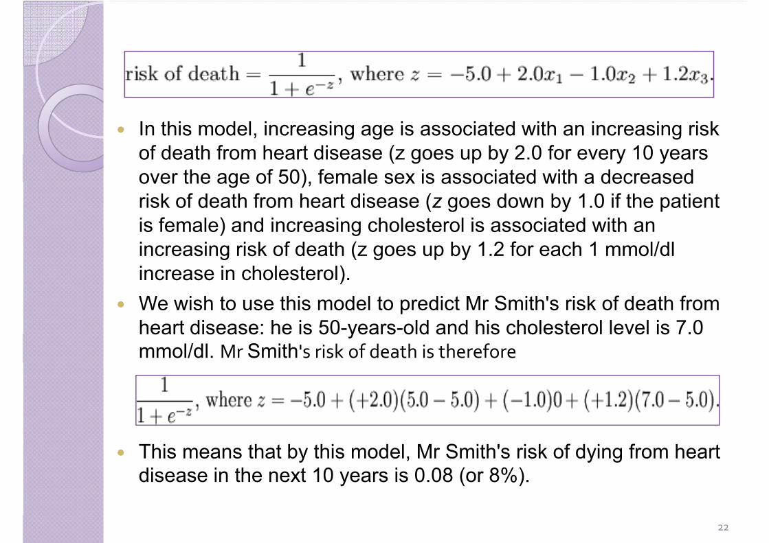
� In this model, increasing age is associated with an increasing risk

of death from heart disease (z goes up by 2.0 for every 10 years

over the age of 50), female sex is associated with a decreased over the age of 50), female sex is associated with a decreased

risk of death from heart disease (z goes down by 1.0 if the patient

is female) and increasing cholesterol is associated with an

increasing risk of death (z goes up by 1.2 for each 1 mmol/dl

increase in cholesterol).

� We wish to use this model to predict Mr Smith's risk of death from

heart disease: he is 50-years-old and his cholesterol level is 7.0

mmol/dl. Mr Smith's risk of death is thereforeMr 's risk of death is therefore

� This means that by this model, Mr Smith's risk of dying from heart

disease in the next 10 years is 0.08 (or 8%).

22

Formal mathematical specificationFormal mathematical specification

� where the numbers of Bernoulli trials ni are known and

the probabilities of success p are unknown. An the probabilities of success pi are unknown. An

example of this distribution is the fraction of seeds (pi)

that germinate after ni are planted.

� The model proposes for each trial (value of i) there is

a set of explanatory variables that might inform the

final probability. These explanatory variables can be

thought of as being in a k vector Xi and the model then

takes the form

23

� The logits of the unknown binomial probabilities (i.e.,

the logarithms of the odds) are modeled as a linear

function of the Xi.

� Note that a particular element of Xi can be set to 1 for � Note that a particular element of Xi can be set to 1 for

all i to yield an intercept in the model.

� The interpretation of the βj parameter estimates is as

the additive effect on the log odds ratio for a unit

change in the jth explanatory variable.

24

� The odds ratio is a measure of effective size particularly

important in logistic regression.

� It is defined as the ratio of the odds of an event occurring in one

group to the odds of it occurring in another group, or to a sample-

based estimate of that ratio. These groups might be men and

women, an experimental group and a control, or any other

dichotomous classification. If the probabilities of the event in each dichotomous classification. If the probabilities of the event in each

of the groups are p (first group) and q (second group), then the

odds ratio is:

� An odds ratio of 1 indicates that the condition or event under

study is equally likely in both groups. An odds ratio greater than study is equally likely in both groups. An odds ratio greater than

1 indicates that the condition or event is more likely in the first

group.. The odds ratio must be greater than or equal to zero. As

the odds of the first group approaches zero, the odds ratio

approaches zero. As the odds of the second group approaches

zero, the odds ratio approaches positive infinity.

25

� For example, suppose that in a sample of 100 men, 90

have drunk wine in the previous week, while in a

sample of 100 women only 20 have drunk wine in the

same period. The odds of a man drinking wine are 90

to 10, or 9:1, while the odds of a woman drinking wine to 10, or 9:1, while the odds of a woman drinking wine

are only 20 to 80, or 1:4 = 0.25:1. Now, 9/0.25 = 36, so

the odds ratio is 36, showing that men are much more

likely to drink wine than women. Using the above

formula for the calculation yields:

� This example also shows how odds ratios can

sometimes seem to overstate relative positions: in this

sample men are 90/20 = 4.5 times more likely to have

drunk wine than women, but have 36 times the odds.

26

� The model has an equivalent formulation

� This functional form is commonly called a single-layer perceptron � This functional form is commonly called a single-layer perceptron

or single-layer artificial neural network. A single-layer neural

network computes a continuous output instead of a step function.

The derivative of pi with respect to X = x1...xk is computed from

the general form:

� easy to take

� where f(X) is an analytic function in X. With this choice, the

single-layer network is identical to the logistic regression model.

This function has a continuous derivative, which allows it to be

used in back-propagation.

27

ExtensionsExtensions

� Extensions of the model cope with multi-category

dependent variables and ordinal dependent variables,

such as polynomial regression. Multi-class such as polynomial regression. Multi-class

classification by logistic regression is known as

multinomial logit modeling. An extension of the logistic

model to sets of interdependent variables is the

conditional random field.

28

Logistic mapLogistic map

� The logistic map is a polynomial mapping, often cited

as an archetypal example of how complex, chaotic

behavior can arise from very simple non-linear

dynamical equations. The map was popularized in a

seminal 1976 paper by the biologist Robert May, in seminal 1976 paper by the biologist Robert May, in

part as a discrete-time demographic model analogous

to the logistic equation first created by Pierre Francois

Verhulst. Mathematically, the logistic map is written

� xn is a number between zero and one, and represents the

population at year n, and hence x0 represents the initial

population (at year 0)

� r is a positive number, and represents a combined rate for

reproduction and starvation. 29

BehaviourBehaviour dependent on dependent on rr� By varying the parameter r, the following behaviour is

observed

� With r between 0 and 1, the population will eventually

die, independent of the initial population.

� With r between 1 and 2, the population will quickly � With r between 1 and 2, the population will quickly

stabilize on the value

� (r-1)/r, independent of the initial population. With r

between 2 and 3, the population will also eventually

stabilize on the same value

� (r-1)/r, but first oscillates around that value for some

time. The rate of convergence is linear, except for r=3, time. The rate of convergence is linear, except for r=3,

when it is dramatically slow, less than linear.

� With r between 3 and (approximately 3.45), the

population may oscillate between two values forever.

These two values are dependent on r.

30

� With r increasing beyond 3.54, the population will

probably oscillate between 8 values, then 16, 32, etc.

The lengths of the parameter intervals which yield the

same number of oscillations decrease rapidly.

� At r approximately 3.57 is the onset of chaos, at the � At r approximately 3.57 is the onset of chaos, at the

end of the period-doubling cascade. We can no longer

see any oscillations. Slight variations in the initial

population yield dramatically different results over

time, a prime characteristic of chaos.

� Most values beyond 3.57 exhibit chaotic behavior, but

there are still certain isolated values of r that appear to there are still certain isolated values of r that appear to

show non-chaotic behavior; these are sometimes

called islands of stability.

� Beyond r = 4, the values eventually leave the interval

[0,1] and diverge for almost all initial values.

31

� A bifurcation diagram summarizes this. The horizontal

axis shows the values of the parameter r while the

vertical axis shows the possible long-term values of x.

� Bifurcation diagram for the Logistic map

32

Ricker modelRicker model� The Ricker model is a classic discrete population

model which gives the expected number (or density)

of individuals at + 1 in generation t + 1 as a function of

the number of individuals in the previous generation,the number of individuals in the previous generation,

� Here r is interpreted as an intrinsic growth rate and k

as the carrying capacity of the environment

� The Ricker model is a limiting case of the Hassell

model which takes the form

33

� Hence, and fortunately, even if we

know very little about the initial state of

the logistic map (or some other the logistic map (or some other

chaotic system), we can still say

something about the distribution of

states a long time into the future, and

use this knowledge to inform decisions

based on the state of the system.based on the state of the system.

34

Back to Practice.Back to Practice.

� Containerized cargo.� Containerized cargo.

� Bulk Cargo.

35

36

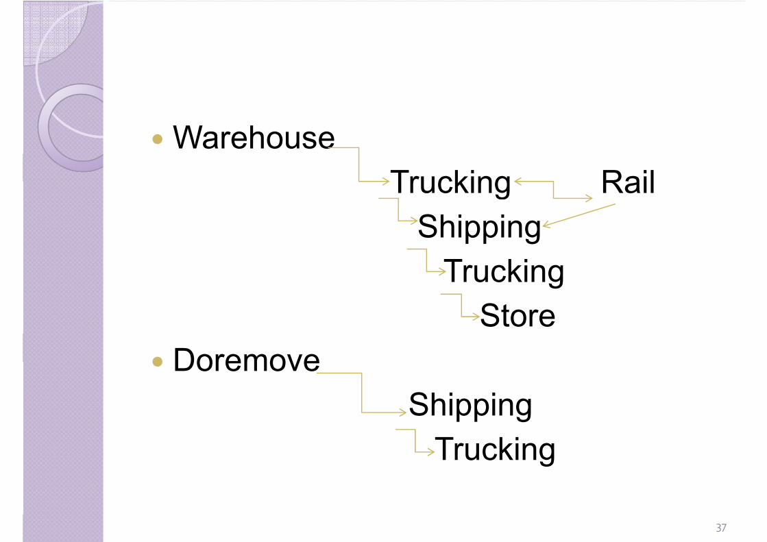
� Warehouse

Trucking Rail Trucking Rail

Shipping

Trucking

Store

� Doremove� Doremove

Shipping

Trucking

37

38

39

Steps of the businessSteps of the business

--first stepsfirst steps

� Chose the business

� Business-plan

� Bank

� Contract of financing� Contract of financing

� Signing with a bank

40

--second stepssecond steps

� Definition

� Searching

41

--third partthird part

� Carry on negotiations with

� Negotiation of all conditions of

contracts on the meetings;

42

--forth partforth part

� open documentary irrevocable

confirmed Letter ofconfirmed Letter of

� Signing the Contract with

� Sending application to the Bank for � Sending application to the Bank for

opening the Letter of Credit to the

Maker – all terms of the letter of Credit

has to be agreed in a Contract with a

Maker;43

--the last onethe last one

� Payments

� Receiving money from your Buyers.

44

45

ReferencesReferences� Brännström A and Sumpter DJ (2005) The role of competition and

clustering in population dynamics. Proc Biol Sci. Oct 7 272(1576):2065-

72

Geritz SA and Kisdi E (2004).

� On the mechanistic underpinning of discrete-time population models with

complex dynamics. J Theor Biol. 2004 May 21;228(2):261-9.

Ricker, WE (1954).

� Stock and recruitment. J ournal of the Fisheries Research Board of

Canada.

� Agresti, Alan. (2002). Categorical Data Analysis. New York: Wiley-

Interscience.

� Amemiya, T. (1985). Advanced Econometrics. Harvard University Press.

Balakrishnan, N. (1991). Handbook of the Logistic Distribution. Marcel � Balakrishnan, N. (1991). Handbook of the Logistic Distribution. Marcel

Dekker, Inc..

� Green, William H. (2003). Econometric Analysis, fifth edition. Prentice

Hall..

� Hosmer, David W.; Stanley Lemeshow (2000). Applied Logistic

Regression, 2nd ed.. New York; Chichester, Wiley.

� http://luna.cas.usf.edu/~mbrannic/files/regression/Logistic.html46

�Thank you for your attention!!

47