lms imagine.lab amesim -...

LMS Imagine.Lab AMESim

Hydraulic Resistance Library Rev 12User’s guide

How to contact LMS Imagine.Lab

www.lmsintl.com Web site

www.lmsintl.com/support Technical support

See here for e-mail addresses for your local office:

www.lmsintl.com/lmsworldwideSales, pricing and general information

+33 4 77 23 60 30 Phone

+33 4 77 23 60 31 Fax

LMS Imagine S.A.7 place des Minimes42300 Roanne - France

Postal address

AMESim® User’s Guides

© Copyright LMS Imagine S.A. 1995-2013

The software described in this documentation is furnished under a license agreement. The software may be used or copied only under the terms of the license agreement. No part of this manual may be photo-copied or reproduced in any form without prior written consent from LMS Imagine S.A.

Trademarks

AMESim® is a registered trademark of LMS Imagine S.A.AMESet® is a registered trademark of LMS Imagine S.A.AMERun® is a registered trademark of LMS Imagine S.A.AMECustom® is a registered trademark of LMS Imagine S.A.LMS Imagine.Lab® is a registered trademark of LMS International N.V.LMS Virtual.Lab Motion® is a registered trademark of LMS International N.V.SysDM® is a registered trademark of LMS International N.V.System Synthesis® is a registered trademark of LMS International N.V.

Other product or brand names are trademarks or registered trademarks of their respective holders.

MMaarrcchh 22001133 TTaabbllee ooff ccoonntteennttss 11//11

TABLE OF CONTENTS 1. Introduction .............................................................................................................................. 1

2. Getting started with the Hydraulic Resistance Library ......................................................... 1

3. Pressures used in AMESim ................................................................................................... 10

3.1. AMESim® standard components ....................................................................................... 10 3.2. Notion of relative and absolute pressures in AMESim ....................................................... 10 3.3. Hydraulic Resistance Library components ........................................................................ 11

4. Modeling a network with Hydraulic Resistance components: important rules ................ 12

5. Tutorial example ..................................................................................................................... 13

6. Formulation of equations and underlying assumptions ..................................................... 19

6.1. Basic equations ................................................................................................................. 19 6.2. Further assumptions .......................................................................................................... 20

7. Reynolds number ................................................................................................................... 21

8. Hydraulic Resistance submodels: classification ................................................................ 23

8.1. Frictional drag category ..................................................................................................... 23 8.2. Local resistance category .................................................................................................. 26 8.3. Frictional and local resistance category ............................................................................ 26 8.4. Plain journal bearing category ........................................................................................... 27

9. Causality in the hydraulic resistance library ....................................................................... 34

10. The connectors: steady state and quasi-steady state problems ..................................... 35

11. References ............................................................................................................................ 36

12. APPENDIX A ......................................................................................................................... 37

13. APPENDIX B ......................................................................................................................... 44

MMaarrcchh 22001133 HHyyddrraauulliicc RReessiissttaannccee LLiibbrraarryy 11//4444

1. Introduction Flow resistance has a strong influence on the design of fluid power circuits in which pressures are relatively low but flow rates are high. This is the reason for the creation of the AMESim® Hydraulic Resistance Library. This library comprises a set of components from which it is easy to model large hydraulic networks, evaluate pressure drops through the elements and, if required, modify the design of the system. Fluids are moved by a difference of pressure. Resistance to flow can be characterized by friction (regular pressure drops) and changes in stream direction or velocity (singular pressure drops). Pressure drops in each hydraulic resistance library component are evaluated based on the Idel'cik [1] formulae and experiment data. Before summarizing the particular characteristics of this library, we present a small tutorial example. Next, rules and advice are given on how to take advantage of the possibilities offered by the hydraulic resistance library. An additional tutorial example is presented. This will introduce some concepts which will lead to a brief description of the background theory. Finally a classification of the submodels is given followed by some more general information. It is assumed that the reader is familiar with the use of AMESim®. If this is not the case, we suggest that you do the exercises in chapter 2 of the AMESim® manual before attempting the examples below.

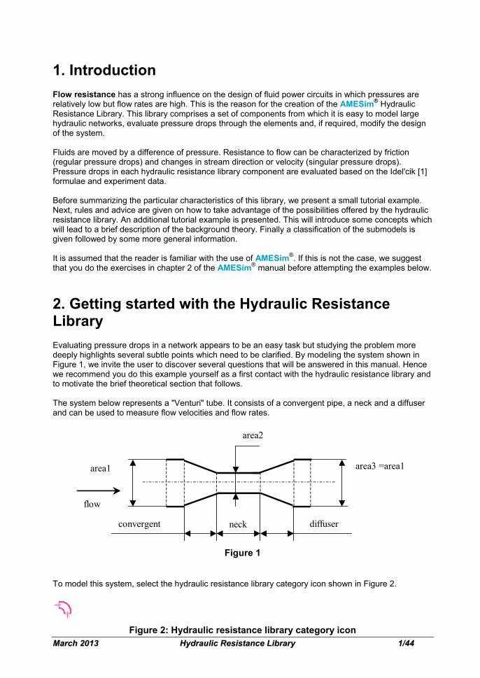
2. Getting started with the Hydraulic Resistance Library Evaluating pressure drops in a network appears to be an easy task but studying the problem more deeply highlights several subtle points which need to be clarified. By modeling the system shown in Figure 1, we invite the user to discover several questions that will be answered in this manual. Hence we recommend you do this example yourself as a first contact with the hydraulic resistance library and to motivate the brief theoretical section that follows. The system below represents a "Venturi" tube. It consists of a convergent pipe, a neck and a diffuser and can be used to measure flow velocities and flow rates.

convergent

neck

area1

area2

area3 =area1

diffuser

flow

Figure 1

To model this system, select the hydraulic resistance library category icon shown in Figure 2.

Figure 2: Hydraulic resistance library category icon


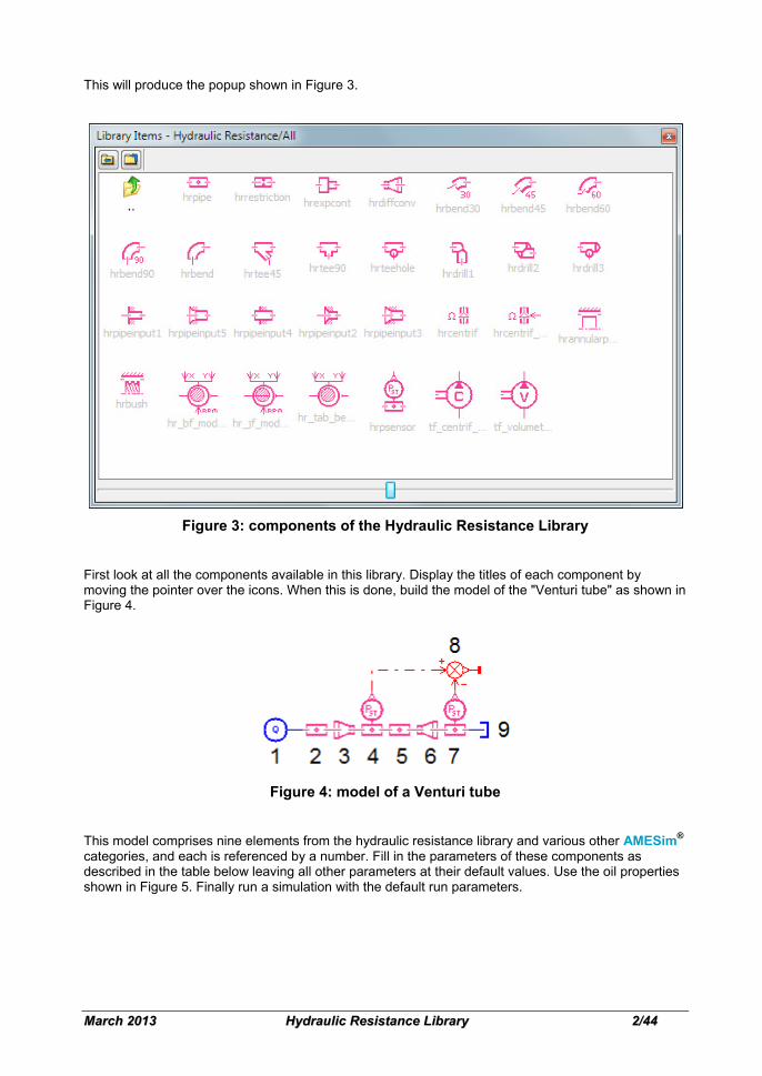
This will produce the popup shown in Figure 3.

Figure 3: components of the Hydraulic Resistance Library

First look at all the components available in this library. Display the titles of each component by moving the pointer over the icons. When this is done, build the model of the "Venturi tube" as shown in Figure 4.

Figure 4: model of a Venturi tube

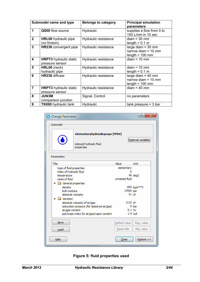
This model comprises nine elements from the hydraulic resistance library and various other AMESim® categories, and each is referenced by a number. Fill in the parameters of these components as described in the table below leaving all other parameters at their default values. Use the oil properties shown in Figure 5. Finally run a simulation with the default run parameters.


Submodel name and type Belongs to category Principal simulation

parameters 1 QS00 flow source Hydraulic supplies a flow from 0 to

150 L/min in 10 sec 2 HRL00 hydraulic pipe

(no friction) Hydraulic resistance diam = 30 mm

length = 0.1 m 3 HR236 convergent pipe Hydraulic resistance large diam = 30 mm

narrow diam = 10 mm length = 100 mm

4 HRPT3 hydraulic static pressure sensor

Hydraulic resistance diam = 10 mm

5 HRL00 (neck) hydraulic pipe

Hydraulic resistance diam = 10 mm length = 0.1 m

6 HR236 diffuser Hydraulic resistance large diam = 40 mm narrow diam = 10 mm length = 100 mm

7 HRPT3 hydraulic static pressure sensor


8 JUN3M comparison junction

Signal, Control no parameters

9 TK000 hydraulic tank Hydraulic tank pressure = 3 bar

Figure 5: fluid properties used


Most of the hydraulic resistance elements do not have state variables. We could describe them as steady state submodels or more precisely as instantaneous submodels. This means that they are assumed to react instantaneously to the pressures applied to them so that they are always in an equilibrium state. The exceptions are submodels such as HRL00. These are very commonly used in hydraulic resistance library systems and they will be described as connection elements. If you look at the variables available for plotting, you will discover that some pressures are described as static pressures and others as total pressures. These terms will be defined precisely in the theoretical section. At this stage we will simply say that the static pressure can be measured by a manometer and the total pressure by a Pitot tube inserted in the flow stream. If the fluid is in motion, total pressure is always greater than static pressure. The difference is due to the motion (kinetic energy) of the moving fluid and is called the dynamic pressure. total pressure = static pressure + dynamic pressure (1) The main point of interest in this example is to observe what happens between the neck and the outlet of the diffuser. If we compare the static pressure in the neck pstat_neck with the static pressure in the diffuser outlet pstat_diffuser we have: diffuserstatneckstat pp __ < (2)

In contrast, if we compare the corresponding total pressures ptot_neck and ptot_diffuser we have: diffusertotnecktot pp __ > (3)

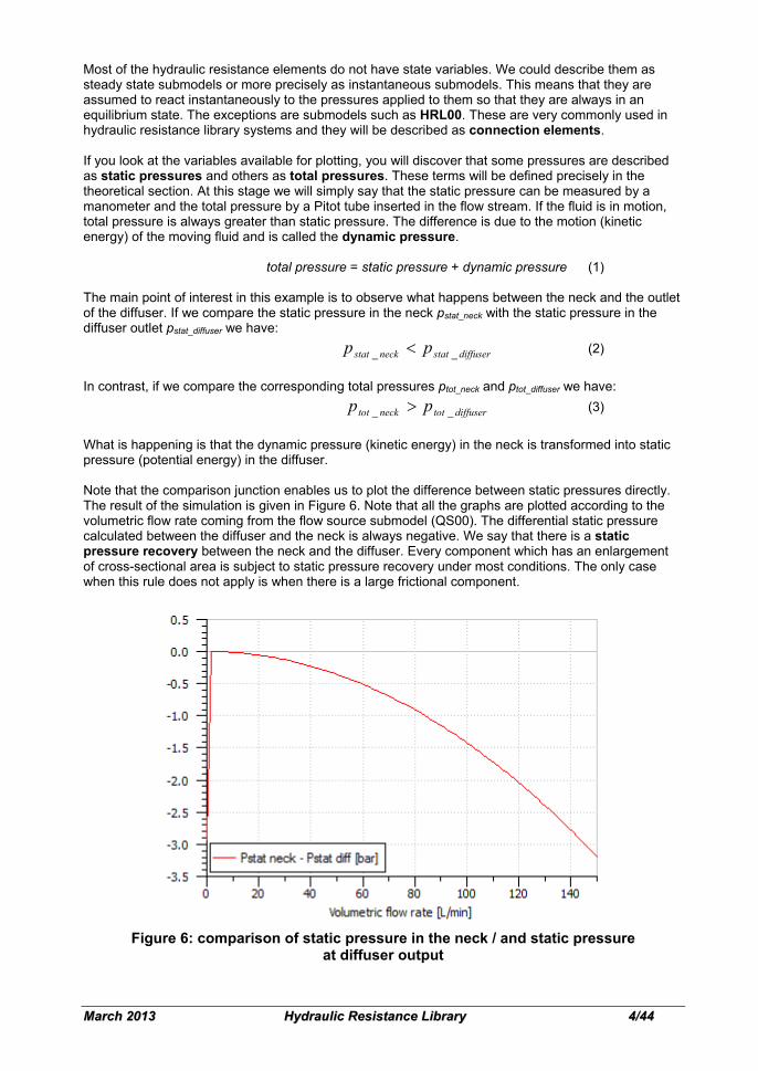
What is happening is that the dynamic pressure (kinetic energy) in the neck is transformed into static pressure (potential energy) in the diffuser. Note that the comparison junction enables us to plot the difference between static pressures directly. The result of the simulation is given in Figure 6. Note that all the graphs are plotted according to the volumetric flow rate coming from the flow source submodel (QS00). The differential static pressure calculated between the diffuser and the neck is always negative. We say that there is a static pressure recovery between the neck and the diffuser. Every component which has an enlargement of cross-sectional area is subject to static pressure recovery under most conditions. The only case when this rule does not apply is when there is a large frictional component.

Figure 6: comparison of static pressure in the neck / and static pressure at diffuser output


In each hydraulic resistance component, total pressures are calculated. If a static pressure is not available, it may be calculated from the total pressure by the hydraulic static pressure sensor in the hydraulic resistance library. In this tutorial example, we will compare the three types of pressure: total pressures, static pressures and dynamic pressures. First we will consider the evolution of total pressures with the flow rate. Bernoulli's formula, which will be studied in detail later in this document, implies that if the flow goes from a point A to a point B in a network: the total pressure at point A is always greater than the total pressure at point B. The total pressure drop between A and B is due to the loss of energy through the elements encountered from point A to point B, and each is characterized by a friction factor.

Figure 7: evolution of total pressures against the volumetric flow rate

In Figure 7, we see the way the three total pressures vary with the flow rate. At the end of the simulation, when the flow rate has reached 150 L/min, the total pressures at convergent pipe inlet, in the neck and at diffuser outlet are respectively, ptot_conv = 5.08 bar, ptot_neck = 4.10 bar and ptot_diff = 3 bar. The last pressure, of course, corresponds to the tank pressure.


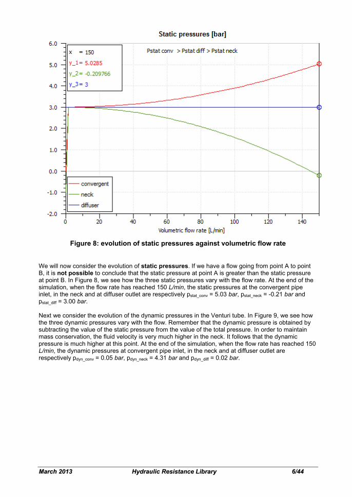
Figure 8: evolution of static pressures against volumetric flow rate

We will now consider the evolution of static pressures. If we have a flow going from point A to point B, it is not possible to conclude that the static pressure at point A is greater than the static pressure at point B. In Figure 8, we see how the three static pressures vary with the flow rate. At the end of the simulation, when the flow rate has reached 150 L/min, the static pressures at the convergent pipe inlet, in the neck and at diffuser outlet are respectively pstat_conv = 5.03 bar, pstat_neck = -0.21 bar and pstat_diff = 3.00 bar. Next we consider the evolution of the dynamic pressures in the Venturi tube. In Figure 9, we see how the three dynamic pressures vary with the flow. Remember that the dynamic pressure is obtained by subtracting the value of the static pressure from the value of the total pressure. In order to maintain mass conservation, the fluid velocity is very much higher in the neck. It follows that the dynamic pressure is much higher at this point. At the end of the simulation, when the flow rate has reached 150 L/min, the dynamic pressures at convergent pipe inlet, in the neck and at diffuser outlet are respectively pdyn_conv = 0.05 bar, pdyn_neck = 4.31 bar and pdyn_diff = 0.02 bar.


Figure 9: evolution of dynamic pressures against volumetric flow rate

Now we can ask why do the flow rates and pressures vary during the simulation? Clearly the flow rate source, which ramps from 0 to 150 L/min in 10 seconds, is a major cause of the variations. There is, however, another factor. You may have noticed that there are two state variables. These are the pressures in the two HRL00 submodels. If you look very carefully at figures 6, 7, 8 and 9 you will find there is some very fast transient behavior at the start of the simulation. This is because the starting value of the pressures was 0 bar whereas the pressure in the tank was 3 bar.


Figure 10: transient behavior due to two pressure state variables

If we run the simulation again over 10-3 seconds with a suitable communication interval (10-4 s), we can see this behavior in detail as shown in Figure 10. Alternatively we can get rid of this behavior by using one of the following two methods: Either by setting the initial value pressure in both HRL00 submodels to 3 bar. Or by running with the option Stabilizing run + Dynamic run + Minimum discontinuity handling. We can get some insight into the nature of the transient behavior resulting from the state variables by doing an eigenvalue analysis. The problem is non-linear and hence the eigenvalues can be expected to vary with time. However, we are only interested in representative values. Therefore we perform a single linear analysis at a time of 5 seconds and examine the eigenvalues. Figure 11 shows the results.

Figure 11: system eigenvalues

We can say that there are two time constants involved, being approximately 10-5 and 10-7 seconds. These are very fast transients. Quite clearly the dominant source of variations in the pressures and flow rates is the flow rate source term. Naturally if we had an extremely long length in HRL00 (e.g. 30 m) or very fast variations in the source term, the state variables would exert a strong influence. We find that it is very common in hydraulic resistance library applications that the eigenvalues of the system (which are due to the state variables) give rise to very small time constants and variations in pressure and flow rate are totally dominated by the source terms.


From this very basic example, the following questions are raised: Which pressure should we work with? It turns out that there are many good reasons for working with total pressure in hydraulic resistance components. As was seen in this first example, if the flow goes from a point A to a point B we know that we always have a loss of total pressure, whereas it is not possible to assert the same with static or dynamic pressures. (Remember the pressure recovery phenomenon.) However, it is often necessary to know the static pressure. Without the static pressure we would not know if cavitation was occurring. Why are there special dynamic connection elements (HRL00 in this example) inserted between hydraulic resistance elements? How do we know if the problem is quasi-steady state? These three questions are extremely important. They are answered in the following sections and the answers constitute the basis for the correct use of the hydraulic resistance library. Therefore, the user is strongly advised to read the next section carefully.


3. Pressures used in AMESim

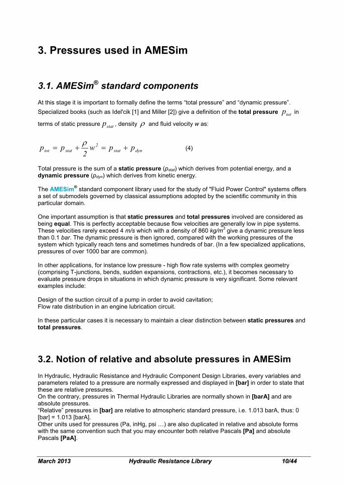
3.1. AMESim® standard components At this stage it is important to formally define the terms “total pressure” and “dynamic pressure”. Specialized books (such as Idel'cik [1] and Miller [2]) give a definition of the total pressure totp in

terms of static pressure statp , density ρ and fluid velocity w as:

dynstat2

stattot ppw2

pp +=+=ρ

(4)

Total pressure is the sum of a static pressure (pstat) which derives from potential energy, and a dynamic pressure (pdyn) which derives from kinetic energy. The AMESim® standard component library used for the study of "Fluid Power Control" systems offers a set of submodels governed by classical assumptions adopted by the scientific community in this particular domain. One important assumption is that static pressures and total pressures involved are considered as being equal. This is perfectly acceptable because flow velocities are generally low in pipe systems. These velocities rarely exceed 4 m/s which with a density of 860 kg/m3 give a dynamic pressure less than 0.1 bar. The dynamic pressure is then ignored, compared with the working pressures of the system which typically reach tens and sometimes hundreds of bar. (In a few specialized applications, pressures of over 1000 bar are common). In other applications, for instance low pressure - high flow rate systems with complex geometry (comprising T-junctions, bends, sudden expansions, contractions, etc.), it becomes necessary to evaluate pressure drops in situations in which dynamic pressure is very significant. Some relevant examples include: Design of the suction circuit of a pump in order to avoid cavitation; Flow rate distribution in an engine lubrication circuit. In these particular cases it is necessary to maintain a clear distinction between static pressures and total pressures.

3.2. Notion of relative and absolute pressures in AMESim In Hydraulic, Hydraulic Resistance and Hydraulic Component Design Libraries, every variables and parameters related to a pressure are normally expressed and displayed in [bar] in order to state that these are relative pressures. On the contrary, pressures in Thermal Hydraulic Libraries are normally shown in [barA] and are absolute pressures. “Relative” pressures in [bar] are relative to atmospheric standard pressure, i.e. 1.013 barA, thus: 0 [bar] = 1.013 [barA]. Other units used for pressures (Pa, inHg, psi …) are also duplicated in relative and absolute forms with the same convention such that you may encounter both relative Pascals [Pa] and absolute Pascals [PaA].


If you are not comfortable with relative units, you may choose to customize your display units (either globally or locally like in the figure here below), see AMESim Reference Manual for details about units management.

Figure 12: Units for pressure in AMESim

3.3. Hydraulic Resistance Library components In hydraulic resistance applications, flow velocities can be much greater than 4 m/s. Velocities of 15 m/s are not uncommon which with a density of 860 kg/m3 gives a dynamic pressure of approximately 1 bar that cannot be ignored. This is particularly true when the system pressure is very low, the influence of the kinetic energy variations then dominates the calculation of the flow resistance. Consider the following example:

V1 V2 = 0Area1

We have a flow coming from a conduit of finite cross-sectional area entering a large (effectively infinite) tank volume. In the pipe, the fluid has a non-zero velocity whereas in the tank the velocity is so small that it can be assumed to be zero. Between the pipe and the tank, all the kinetic energy (dynamic pressure) of the fluid is transformed into potential energy (static pressure). In the pipe, the dynamic pressure dominates, whereas in the tank, it is the static pressure. It is obvious that the flow velocity is extremely important and therefore we must make a clear distinction between the different types of pressure. We could perform calculations and display pressure results as static pressure or total pressure. Generally it is easier to formulate the equation using total pressure and Idel'cik [1] uses total pressure in his formulae and tables. Hence in the hydraulic resistance library most calculations use total pressure and total pressures are available for plotting. In the rest of this document all pressures are total pressures unless specified otherwise.


4. Modeling a network with Hydraulic Resistance components: important rules This section will detail the important rules that must be respected to model a network correctly with hydraulic resistance library components. • In hydraulic resistance library components, pressure drop calculations are valid only for liquids (or other fluids as long as they can be considered as not compressible). • Building the network: It is better if the user builds the system slowly and runs a simulation after each portion of circuit is added. This normally leads to a better understanding of the system and the results. It is also less likely that the parameter settings will be forgotten. Five connection components can be used, these are HRL00 and HRL01 (compressibility line), HRL03 and HRL04 (compressibility + friction line) and HRCE0 (compressibility + friction + centrifugal effect). These components are described in appendix A. The user must always make the link between two hydraulic resistance components with one of these components. Sometimes when sketching the network, it appears that its structure does not allow you to connect two components because they are not facing each other or because they are too far from each other. In these particular cases, use AMESim® DIRECT CONNECTION lines.

Figure 13: small network example showing that each hydraulic resistance library component has all ports connected to a hydraulic pipe icon

• The user must always remember that, unless otherwise stated, the pressures displayed in hydraulic resistance library components are total pressures. • As previously seen, bend submodels as well as the diffuser submodel do not take into account the frictional drag pressure drop. Normally the local resistance factor is much more important. If you want to include the frictional drag pressure drop, remember that, in a network, a bend is connected at both ports to connection line submodels. Ensure that HRL03 (or HRL04) is used and take the frictional drag effects in the bend into account by increasing the length of the HRL03 (or HRL04) connection line preceding the bend by the value of the bend length.


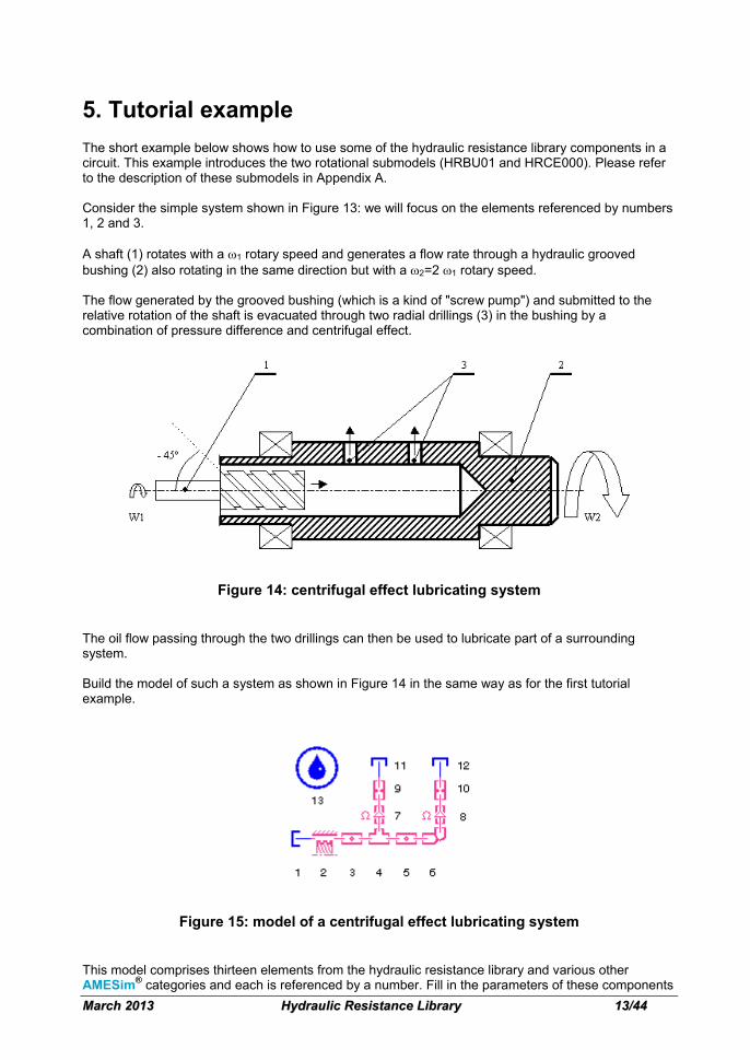
5. Tutorial example The short example below shows how to use some of the hydraulic resistance library components in a circuit. This example introduces the two rotational submodels (HRBU01 and HRCE000). Please refer to the description of these submodels in Appendix A. Consider the simple system shown in Figure 13: we will focus on the elements referenced by numbers 1, 2 and 3. A shaft (1) rotates with a ω1 rotary speed and generates a flow rate through a hydraulic grooved bushing (2) also rotating in the same direction but with a ω2=2 ω1 rotary speed. The flow generated by the grooved bushing (which is a kind of "screw pump") and submitted to the relative rotation of the shaft is evacuated through two radial drillings (3) in the bushing by a combination of pressure difference and centrifugal effect.

Figure 14: centrifugal effect lubricating system

The oil flow passing through the two drillings can then be used to lubricate part of a surrounding system. Build the model of such a system as shown in Figure 14 in the same way as for the first tutorial example.

Figure 15: model of a centrifugal effect lubricating system

This model comprises thirteen elements from the hydraulic resistance library and various other AMESim® categories and each is referenced by a number. Fill in the parameters of these components


as described in the table below. Use the default fluid properties and run a simulation with the default run parameters.

The component HRBU01 is an asymmetrical submodel and thus you must pay attention to its orientation in your system.

Submodel name and type Belongs to category

Principal simulation parameters

1 TK000 hydraulic tank Hydraulic Tank pressure = 1 bar 2 HRBU01 hydraulic

grooved bushing Hydraulic resistance rotary speed of bushing =

2×w1 rotary speed of shaft = w1 groove acute angle = -45°

3 & 5

HRL03 hydraulic pipes with friction and compressibility

Hydraulic resistance diam = 35 mm length = 0.015 m

4 HR206 hydraulic T-junction

Hydraulic resistance diam1 = 10 mm diam23 = 35 mm

6 HR22B 90 deg. intersecting holes


7 & 8

HRCE000 hydraulic pipe with centrifugal effects

Hydraulic resistance diam = 10 mm inlet position = 17.5 mm outlet position = 37.5 mm rotary speed = 2×w1

9 & 10

HR220 hydraulic orifice Hydraulic resistance Default

11 & 12

TK000 hydraulic tanks Hydraulic Tank pressures = 1 bar

13 FP04 fluid properties Hydraulic Default ω1 must be set as a global parameter (in Parameter mode, Parameters > Global parameters). Component 2 is a hydraulic grooved bushing. In this submodel, the calculated flow rate is a function of two important parameters which are the "rotary speed of bushing [rev/min]" and the "rotary speed of shaft [rev/min]". Component 7 (and 8) is a hydraulic pipe with centrifugal effects. In this submodel, the computed pressures are functions of a "rotary speed [rev/min]" and other parameters which do not concern us here. In the model of the "centrifugal effect lubricating system", suppose we want to supply for component 2 rotary speed of bushing = 4000 rev/min = ω2 = 2 ω1 rotary speed of shaft = 2000 rev/min = ω1 and for components 7 and 8 - rotary speed = 4000 rev/min = ω2 = 2 ω1. We can then set a global parameter with the name 'ω1' of the speed to share with components 2, 7 and 8 and its value to 2000 as shown in Figure 15.


Figure 16: global parameters setup

When filling in the parameters of components 2 and 7, we call the name of the global parameter as shown in Figure 16 and Figure 17 in the parameters concerned. It is also possible to supply an expression which is a function of the name of the shared parameter (for instance: 2 ω1).

Figure 17: parameters of submodel HRBU01


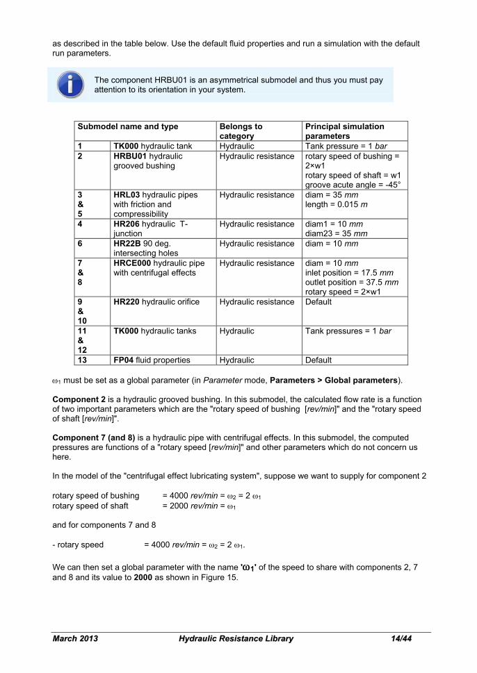
Figure 18: parameters of submodel HRCE000

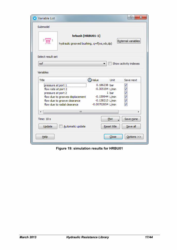
Advantages of using global parameters: First it is necessary to remind the user that the use of global parameters is optional. The use of global parameters becomes essential when working on a network comprising several HRBU01 and HRCE00 submodels with rotary speeds depending on one rotary speed or on functions of one rotary speed. Indeed, if the user wants to run simulations for several values of the rotary speed specified in the global parameters, he only has to change the value in the global parameters, and not in every individual submodel. Going back to the simulation, we display the results in component 2 and component 7 as shown in Figure 18 and Figure 19.


Figure 19: simulation results for HRBU01


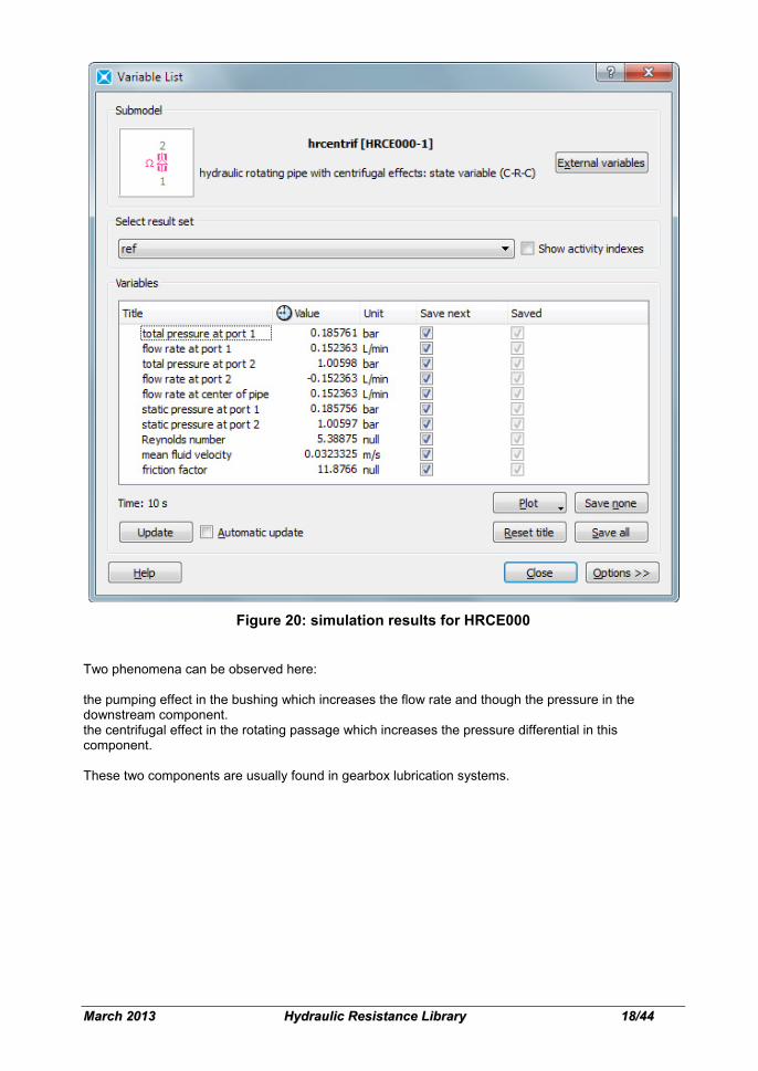
Figure 20: simulation results for HRCE000

Two phenomena can be observed here: the pumping effect in the bushing which increases the flow rate and though the pressure in the downstream component. the centrifugal effect in the rotating passage which increases the pressure differential in this component. These two components are usually found in gearbox lubrication systems.


6. Formulation of equations and underlying assumptions

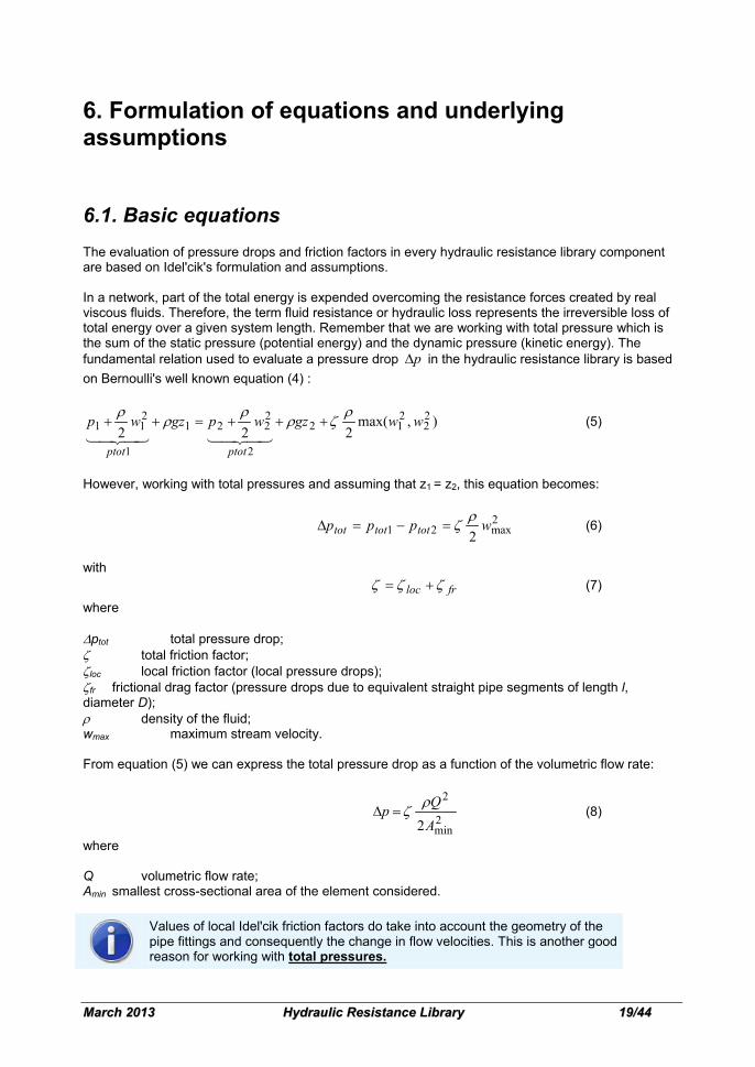
6.1. Basic equations The evaluation of pressure drops and friction factors in every hydraulic resistance library component are based on Idel'cik's formulation and assumptions. In a network, part of the total energy is expended overcoming the resistance forces created by real viscous fluids. Therefore, the term fluid resistance or hydraulic loss represents the irreversible loss of total energy over a given system length. Remember that we are working with total pressure which is the sum of the static pressure (potential energy) and the dynamic pressure (kinetic energy). The fundamental relation used to evaluate a pressure drop p∆ in the hydraulic resistance library is based on Bernoulli's well known equation (4) :

),max(222

22

212

2

2221

1

211 wwgzwpgzwp

ptotptot

ρζρ

ρρ

ρ+++=++

(5)

However, working with total pressures and assuming that z1 = z2, this equation becomes:

2max21 2

wppp tottottotρζ=−=∆ (6)

with frloc ζζζ += (7)

where ∆ptot total pressure drop; ζ total friction factor; ζloc local friction factor (local pressure drops); ζfr frictional drag factor (pressure drops due to equivalent straight pipe segments of length l, diameter D); ρ density of the fluid; wmax maximum stream velocity. From equation (5) we can express the total pressure drop as a function of the volumetric flow rate:

2min

2

2AQp ρζ=∆ (8)

where Q volumetric flow rate; Amin smallest cross-sectional area of the element considered.

Values of local Idel'cik friction factors do take into account the geometry of the pipe fittings and consequently the change in flow velocities. This is another good reason for working with total pressures.


Every hydraulic resistance library component uses equation (8). This equation is used to compute the volumetric flow rate from the pressure drop.

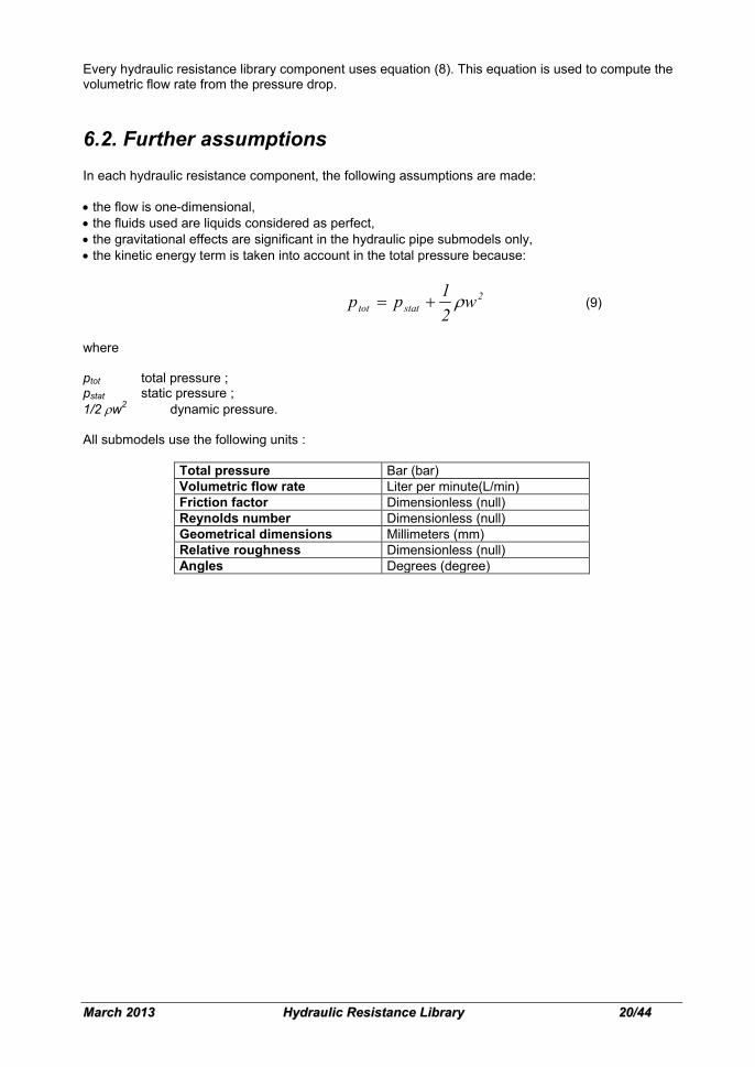
6.2. Further assumptions In each hydraulic resistance component, the following assumptions are made: • the flow is one-dimensional, • the fluids used are liquids considered as perfect, • the gravitational effects are significant in the hydraulic pipe submodels only, • the kinetic energy term is taken into account in the total pressure because:

2stattot w

21pp ρ+= (9)

where ptot total pressure ; pstat static pressure ; 1/2 ρw2 dynamic pressure. All submodels use the following units :

Total pressure Bar (bar) Volumetric flow rate Liter per minute(L/min) Friction factor Dimensionless (null) Reynolds number Dimensionless (null) Geometrical dimensions Millimeters (mm) Relative roughness Dimensionless (null) Angles Degrees (degree)


7. Reynolds number The flow regimes of a liquid or gas can be laminar or turbulent. Laminar flow is stable, the stream layers move without mixing with each other. The turbulent regime is characterized by a random displacement of finite masses mixing strongly with each other. In classic fluid power hydraulic applications, flow is predominately laminar or transitional. In applications using the hydraulic resistance library turbulent flow is also common. It is known that the flow regime depends on the relationship between the inertia and viscosity forces (internal friction) in the stream, which can be expressed by a dimensionless number, the Reynolds number given by:

νν .

..Re

h

hhA

DQDw== (10)

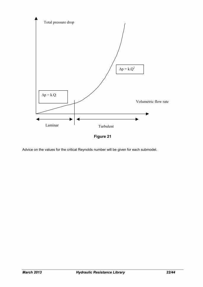
where w maximum stream velocity ; Dh hydraulic diameter ; ν kinematic viscosity; Ah hydraulic cross-sectional area. In the rest of this document the Reynolds number at which the transition between laminar and turbulent flow occurs will be called the critical Reynolds number. This is not an absolute constant but its value in a component can vary considerably with the geometry. Every submodel of the hydraulic resistance library takes into account laminar and turbulent regimes and the following assumptions are made: When the flow is laminar, the total pressure drop is proportional to the volumetric flow rate. When the flow is turbulent, the total pressure drop is proportional to the square of the volumetric flow rate. Figure 20 shows the way laminar and turbulent regimes are taken into account in hydraulic resistance submodels. There are two types of submodel in the hydraulic resistance library which differ in the way they deal with the critical Reynolds number: Type 1: These submodels use Idel'cik friction factor tables so that the critical Reynolds number is not used explicitly because it is already taken into account in the tables. Type 2: These submodels have fixed friction factors supplied by the user and in addition the critical Reynolds number is required. The user will have to supply a consistent value for the critical Reynolds number depending on the nature of the fitting.


Total pressure drop

∆p = k.Q

Volumetric flow rate

Laminar Turbulent

∆p = k.Q2

Figure 21

Advice on the values for the critical Reynolds number will be given for each submodel.


8. Hydraulic Resistance submodels: classification A further classification of submodels in the hydraulic resistance library is: Category 1: Submodels which compute frictional drag. Category 2: Submodels which compute local resistance. Category 3: Submodels which compute frictional drag and local resistance. Category 4: Submodels of plain journal bearings The following paragraphs describe these hydraulic resistance submodel categories.

8.1. Frictional drag category Submodels belonging to this category are used to model resistance to flow in straight tubes and conduits. The pressure losses along a straight tube of constant cross-sectional area are calculated from the Darcy-Weisbach equation (11):

2

2

h A2Q

DlpΔ

min

. ρλ= (11)

where: λ friction coefficient of the segment of relative unit length l/Dh =1; Dh hydraulic or equivalent diameter; l length of flow segment. For this type of submodel, in order to make an analogy with equation (6), the total friction factor ζ is given by:

hD

lλζ = (12)

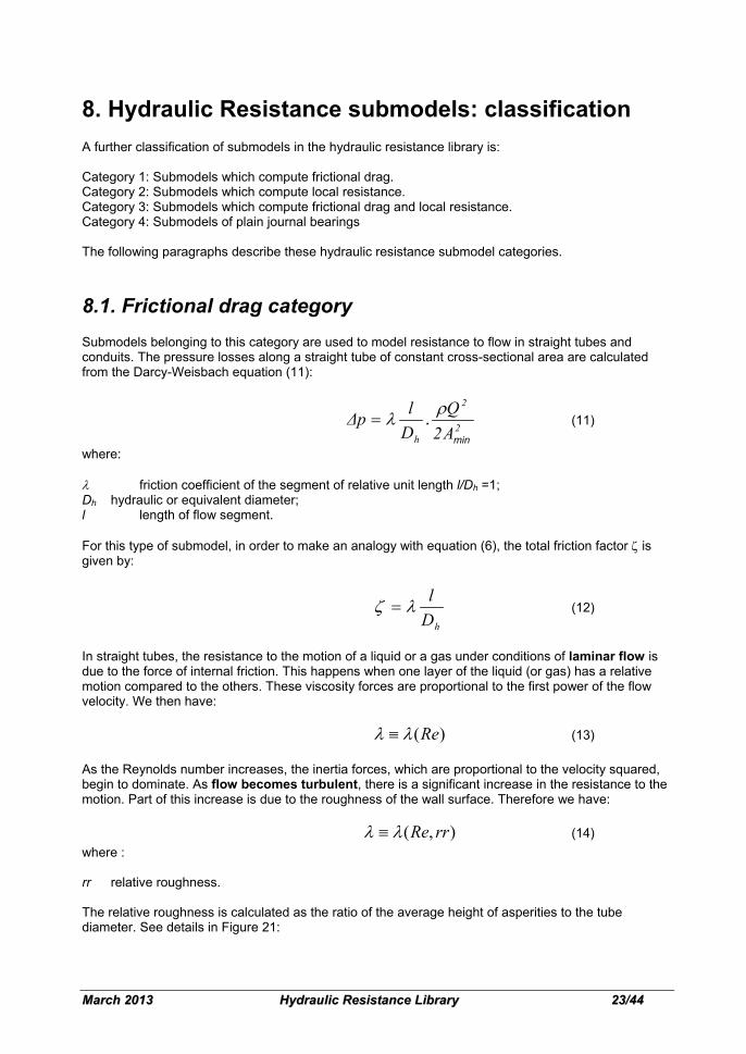
In straight tubes, the resistance to the motion of a liquid or a gas under conditions of laminar flow is due to the force of internal friction. This happens when one layer of the liquid (or gas) has a relative motion compared to the others. These viscosity forces are proportional to the first power of the flow velocity. We then have: )(Reλλ ≡ (13) As the Reynolds number increases, the inertia forces, which are proportional to the velocity squared, begin to dominate. As flow becomes turbulent, there is a significant increase in the resistance to the motion. Part of this increase is due to the roughness of the wall surface. Therefore we have: ),( rrReλλ ≡ (14) where : rr relative roughness. The relative roughness is calculated as the ratio of the average height of asperities to the tube diameter. See details in Figure 21:


l

Dh

∆

Figure 22: relative roughness definition

The relative roughness of a pipe is given by:

hDΔrr = (15)

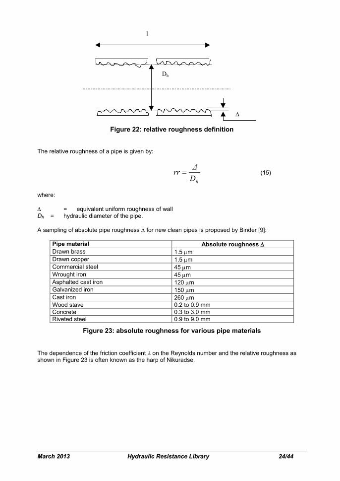
where: ∆ = equivalent uniform roughness of wall Dh = hydraulic diameter of the pipe. A sampling of absolute pipe roughness ∆ for new clean pipes is proposed by Binder [9]:

Pipe material Absolute roughness ∆ Drawn brass 1.5 µm Drawn copper 1.5 µm Commercial steel 45 µm Wrought iron 45 µm Asphalted cast iron 120 µm Galvanized iron 150 µm Cast iron 260 µm Wood stave 0.2 to 0.9 mm Concrete 0.3 to 3.0 mm Riveted steel 0.9 to 9.0 mm

Figure 23: absolute roughness for various pipe materials

The dependence of the friction coefficient λ on the Reynolds number and the relative roughness as shown in Figure 23 is often known as the harp of Nikuradse.


Figure 24: evolution of the frictional drag factor with the Reynolds number and the relative roughness The submodels in the hydraulic resistance library found in this category are:

HRL02A / HRL02B HRL03 / HRL04 HRL030 / HRL031

Hydraulic pipes with Compressibility + frictional effects

HRCE000 Hydraulic pipe with centrifugal effects

HR234 Hydraulic annular pipe (relative roughness does not have any influence because in this submodel, the flow is supposed always to be laminar).


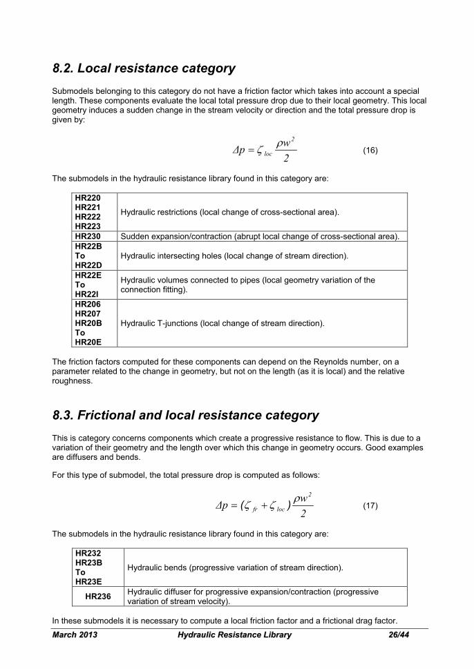
8.2. Local resistance category Submodels belonging to this category do not have a friction factor which takes into account a special length. These components evaluate the local total pressure drop due to their local geometry. This local geometry induces a sudden change in the stream velocity or direction and the total pressure drop is given by:

2wpΔ

2

locρζ= (16)

The submodels in the hydraulic resistance library found in this category are:

HR220 HR221 HR222 HR223

Hydraulic restrictions (local change of cross-sectional area).

HR230 Sudden expansion/contraction (abrupt local change of cross-sectional area). HR22B To HR22D

Hydraulic intersecting holes (local change of stream direction).

HR22E To HR22I

Hydraulic volumes connected to pipes (local geometry variation of the connection fitting).

HR206 HR207 HR20B To HR20E

Hydraulic T-junctions (local change of stream direction).

The friction factors computed for these components can depend on the Reynolds number, on a parameter related to the change in geometry, but not on the length (as it is local) and the relative roughness.

8.3. Frictional and local resistance category This is category concerns components which create a progressive resistance to flow. This is due to a variation of their geometry and the length over which this change in geometry occurs. Good examples are diffusers and bends. For this type of submodel, the total pressure drop is computed as follows:

2wpΔ

2

locfrρζζ )( += (17)

The submodels in the hydraulic resistance library found in this category are:

HR232 HR23B To HR23E

Hydraulic bends (progressive variation of stream direction).

HR236 Hydraulic diffuser for progressive expansion/contraction (progressive variation of stream velocity).

In these submodels it is necessary to compute a local friction factor and a frictional drag factor.


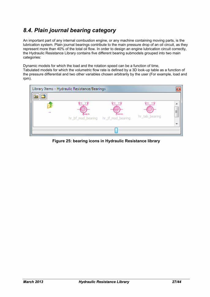
8.4. Plain journal bearing category An important part of any internal combustion engine, or any machine containing moving parts, is the lubrication system. Plain journal bearings contribute to the main pressure drop of an oil circuit, as they represent more than 40% of the total oil flow. In order to design an engine lubrication circuit correctly, the Hydraulic Resistance Library contains five different bearing submodels grouped into two main categories: Dynamic models for which the load and the rotation speed can be a function of time, Tabulated models for which the volumetric flow rate is defined by a 3D look-up table as a function of the pressure differential and two other variables chosen arbitrarily by the user (For example, load and rpm).

Figure 25: bearing icons in Hydraulic Resistance library


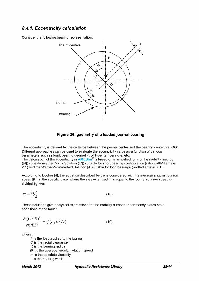
8.4.1. Eccentricity calculation

Consider the following bearing representation:

Figure 26: geometry of a loaded journal bearing

The eccentricity is defined by the distance between the journal center and the bearing center, i.e. OO’. Different approaches can be used to evaluate the eccentricity value as a function of various parameters such as load, bearing geometry, oil type, temperature, etc. The calculation of the eccentricity in AMESim® is based on a simplified form of the mobility method ([4]) considering the Ocvirk Solution ([7]) suitable for short bearing configuration (ratio width/diameter < 1) and the Warner-Sommerfeld Solution [4] suitable for long bearings (width/diameter > 1). According to Booker [4], the equation described below is considered with the average angular rotation speedϖ . In the specific case, where the sleeve is fixed, it is equal to the journal rotation speed ω divided by two:

2ωϖ = (18)

Those solutions give analytical expressions for the mobility number under steady states state conditions of the form :

)/,()/( 2

DLfLD

RCF εϖµ

= (19)

where : F is the load applied to the journal C is the radial clearance R is the bearing radius ϖ is the average angular rotation speed m is the absolute viscosity L is the bearing width

O

O’

e

ω

line of centers

Φ

bearing

journal

F


D is the bearing diameter e is the eccentricity ε is the eccentricity ratio, ε = e / C The function f(ε,L/D) can have several forms depending on the assumptions made regarding the extent of the oil film. Usually, we assume that there is an oil film rupture along the bearing circumference after a certain angle from the feed hole. In this library, the default assumption is a film extent of π radians but user can choose to work with the ideal case of a complete film (2π extent). Since the above considerations suppose steady state conditions, it is important to notice that the all submodels present in the library are based on a quasi-steady-state approach.

8.4.2. Bearing submodels: Assumptions

All the submodels are isothermal and do not take into account any temperature variation (constant viscosity), The rotational velocity considered is the speed of the journal relative to the bearing (sleeves or housings are fixed), All the angles are expressed starting from the vertical axis in the direction of the journal rotation Submodels are based on a quasi-steady-state approach.

8.4.3. Examples with bearings

8.4.3.1. Setting the load and the speed in dynamic submodels

Some submodels use three input signal ports for the settings of load and speed conditions. These ports are labeled X and Y for the load and RPM for the rotation speed. With the use of signal ports, these inputs can be set as constants, functions of time and/or other parameters, outputs from look up tables, etc. Speed is supplied in Revolutions Per Minute [rev/min]. The load is defined by its intensity [N] and its direction [degree]. The user has the choice of the system of coordinates for the load definition, either rectangular or polar. The choice of the system is set in the popup window as seen in Figure 26.


Figure 27: selection of the coordinates system

for the rectangular system, X and Y correspond to Fx and Fy, the projections of the vector F on X and Y axes as shown in the following figure:

Figure 28: definition of load using rectangular and polar coordinates systems


Using this method, the intensity of the load is calculated by: 22YX FFF +=

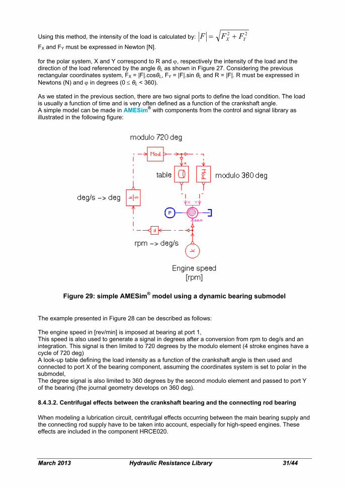
FX and FY must be expressed in Newton [N]. for the polar system, X and Y correspond to R and ϕ, respectively the intensity of the load and the direction of the load referenced by the angle θL as shown in Figure 27. Considering the previous rectangular coordinates system, FX = |F|.cosθL, FY = |F|.sin θL and R = |F|. R must be expressed in Newtons (N) and ϕ in degrees (0 ≤ θL < 360). As we stated in the previous section, there are two signal ports to define the load condition. The load is usually a function of time and is very often defined as a function of the crankshaft angle. A simple model can be made in AMESim® with components from the control and signal library as illustrated in the following figure:

Figure 29: simple AMESim® model using a dynamic bearing submodel

The example presented in Figure 28 can be described as follows: The engine speed in [rev/min] is imposed at bearing at port 1, This speed is also used to generate a signal in degrees after a conversion from rpm to deg/s and an integration. This signal is then limited to 720 degrees by the modulo element (4 stroke engines have a cycle of 720 deg) A look-up table defining the load intensity as a function of the crankshaft angle is then used and connected to port X of the bearing component, assuming the coordinates system is set to polar in the submodel, The degree signal is also limited to 360 degrees by the second modulo element and passed to port Y of the bearing (the journal geometry develops on 360 deg).

8.4.3.2. Centrifugal effects between the crankshaft bearing and the connecting rod bearing

When modeling a lubrication circuit, centrifugal effects occurring between the main bearing supply and the connecting rod supply have to be taken into account, especially for high-speed engines. These effects are included in the component HRCE020.


The following Figure 29 shows an example of main bearing and connecting rod bearing lubrication paths.

Figure 30: example of bearing lubrication

To model such a system, the user can represent the main bearing and the connecting rod bearing on parallel branches and add centrifugal effects with HRCE020 on the connecting rod bearing branch. Finally, the AMESim® model is built as shown in Figure 30.

Figure 31: example of bearing lubrication model

Figure 31 represents the flow rates in the main bearing and in the connecting rod bearing as a function of the pressure differential.

Connecting rod

Main Bearing Main Bearing

Crankshaft


Figure 32: Characteristics Q(dP) of the bearing lubrication model

8.4.3.3. Example: Complete oil circuit

The sketch in Figure 32 represents a complete lubrication circuit, including main crankshaft bearings, connecting rod bearings and cam bearings, piston cooling jets, etc.

Figure 33: Cylinder engine lubrication circuit


9. Causality in the hydraulic resistance library What do we mean by causality? Causality is the way we treat the equations in a submodel. In a two-port hydraulic resistance component, three variables are involved which are the pressure at port 1 (p1), the pressure at port 2 (p2) and the volumetric flow rate (q) through the component. Using the same basic equation we can manipulate it to produce three distinct submodels: compute q from p1 and p2, compute p1 from q and p2, compute p2 from q and p1. We say that the three submodels have different causality. In order to produce an AMESim® submodel, the usual Bernoulli's formulation (see equation (8) page 20) used in Idel'cik is manipulated so as to compute the volumetric flow rate Q as a function of the differential pressure ∆p. This means that p1 and p2 are inputs of the submodel which returns the flow rate as an output. This causality implies we cannot connect two hydraulic resistance components together directly. Instead we insert a connection component between them. This computes the pressure between each hydraulic resistance component. An example of this is given below where a typical hydraulic resistance submodel is attached to two connection submodels.

There are six connection submodels which are given designations HRL00, HRL01, HRL03, HRL04, HRL30 and HRL31 which are associated with the icon:

and HRCE000, HRCE100 which are associated with these icons:

These submodels are more fully described in Appendix A.


10. The connectors: steady state and quasi-steady state problems For HRL01 the basic equation is implemented by adjusting the pressure to force the following residual to zero: Qε ∑= (20)

where∑Q is the incoming flow rate. It is clear that setting the residual to zero is equivalent to the

following constraint equation: 0Q =∑ (21)

which is precisely what we want and we describe this as the steady state regime. This equation is not trivial to solve when there is a large hydraulic network and failure is possible. In the first example we showed that the problem was quasi-steady state. By this we mean that the time constants that are introduced by the state variables are so fast that the source terms totally dominate the results. When this happens, if we examine the two flow rates we find that ∑Q is

extremely close to zero. The only exception is at the start of the simulation when we have bad starting values. This is not a problem because we can ignore the results in the first few milliseconds of the simulation or better use the Stabilizing run + dynamic run option. We must now state clearly how we can determine if the problem is quasi-steady state. First we note that the only state variables in the hydraulic resistance library are in the connection elements and they all use the bulk modulus. No other hydraulic resistance elements use the bulk modulus. If we increase the bulk modulus (by a factor of 2, 5 or even 10), the eigenvalues will change and time constants will be reduced. If there are no significant differences in the results, the problem is quasi-steady state. If there are significant differences, you are outside the scope of validity of the library. For HRL00 the equation is implemented as an explicit ordinary differential equation with:

QVB

dtdP ∑= (22)

But here the pipe length cannot be set to zero. HRL03 and HRL04 are similar but include a pressure drop due to friction. HRL03 uses an explicit state variable but HRL04 uses an implicit state. HRCE00 is similar to HRL03 but the pipe is supposed to be rotating so that the flow rate is driven partly by a pressure difference and partly due to a centrifugal effect. When working in the quasi-steady state regime, to avoid a significant dynamic transient behavior due to bad starting values, use the option "Stabilizing run + dynamic run".


11. References [Ref. 1] I.E. Idel'cik, “Handbook of Hydraulic Resistance”, 3rd Edition, Begell House Inc.,

1996. [Ref. 2] D.S. Miller, “Internal Flow systems”, 2nd Edition, Amazon Technology, 1989. [Ref. 3] Jacques Faisandier, “Mécanismes oléo-hydrauliques”, Editions Dunod, 1987. [Ref. 4] [Ref. 5] J.F. Booker, “Dynamically Loaded Journal Bearings: Mobility Method of Solution”,

Trans. ASME Journal of Basic Engineering, Sept. 1965, pp 537-546 [Ref. 6] [Ref. 7] M.A. Mian, “Design and Analysis of Engine Lubrication Systems”, SAE paper

970637 pp 219-227, Ricardo Consulting Engineers Ltd. [Ref. 8] [Ref. 9] F.A. Martin, “Feed Pressure Flow in Plain Journal Bearings”, ASLE Transactions,

July 1983, pp 381-392 [Ref. 10] [Ref. 11] G.B. Dubois & F.W. Ocvirk, “Analytical and Experimental Evaluation of Short-

Bearing Approximation for Full Journal Bearings”, NACA report 1157, 1953, pp 1199-1230

[Ref. 12] [Ref. 13] G.B. Dubois & F.W. Ocvirk, “Relation of Journal Bearing Performance to Minimum

oil-film thickness”, NACA TN 4223, April 1958 [Ref. 14] [Ref. 15] R.C. Binder, “Fluid Mechanics”. 3rd Edition, 3rd Printing. Prentice-Hall, Inc.,

Englewood Cliffs, NJ. 1956 [Ref. 16] [Ref. 17] [Ref. 18]


12. APPENDIX A Description of hydraulic resistance submodels This version of the Hydraulic Resistance library includes about 30 submodels. It is useful to present a brief survey of the Hydraulic Resistance library submodels, their aim and their limitations. Each hydraulic resistance library icon is displayed, followed by a description of the corresponding submodels. For more detailed information, please refer to the HTML documentation or the submodel description directly in AMESim.

A.1. Hydraulic pipe icon

With standard AMESim® hydraulic systems, pipes and hoses are represented by lines. This conforms to the normal drawing standards for hydraulic systems. In the hydraulic resistance library the alternative icon shown above exists. There are six submodels associated with this icon. They are very similar to the standard line submodels HL000 and HL03 but compute total pressure and static pressure separately. Use this icon and its corresponding submodels rather than the standard AMESim® pipe submodels. HRL00 (pressure is an explicit state variable) and HRL01 (pressure is an implicit state variable). These are submodels of hydraulic pipes in which the volume is calculated from the length and diameter and pressure dynamic is modeled. Frictional effects are ignored. If the pipe length is set to zero in HRL01, the equation solved is purely algebraic. In all other circumstances an ordinary differential equation is solved. This will create a time constant and this should be small enough to give quasi-steady state problem. HRL03 (pressures are explicit state variables) and HRL04 (pressures are implicit state variables). These are submodels of hydraulic pipes which take into account both the compressibility and the frictional effects. HRL30 (pressures are explicit state variables) and HRL31 (pressures are implicit state variables). These submodels of hydraulic pipes which take into account both the compressibility and the frictional effects are similar to HRL03 and HRL31 respectively. The difference comes from the use of both a hydraulic diameter and a cross-sectional area as parameters. They are thus not restricted to a circular section of the pipe. When networks are badly conditioned or use lots of submodels which read tables and thus create a lot of discontinuities, using HRL01 and HRL04 can lead to slow runs and therefore it is worth using HRL00 and HRL03 connection elements. Remember that one of these four connection submodels must be used whenever you wish to connect two other hydraulic resistance components.


A.2. Hydraulic restriction icon

Four submodels are associated with this icon. HR220 This is a submodel of a hydraulic orifice. It can have laminar or turbulent characteristics and the switch is made at a user-defined critical Reynolds number (normally in the range 10 to 200). The friction factor supplied is constant during the simulation. This is the classical sharp edge orifice. HR221 This is a submodel of a hydraulic orifice. It can have laminar or turbulent characteristics and the switch is made at a user-defined critical flow number. There are two usage modes: 1. the user only supplies a flow rate and a corresponding pressure drop. 2. the user supplies an equivalent orifice diameter and a maximum flow coefficient. HR0222 This is a submodel of a hydraulic orifice. Use this orifice if you have a table or an equation relating the flow rate and the corresponding pressure drop as q = f(dp). HR0223 This is a submodel of a hydraulic orifice. It has the same characteristics as HR221 but there are fewer parameters to set. The difference is that the critical flow number (lamc = 100) and the maximum flow coefficient (cqmax = 1.0) are hard coded. Therefore, the user only has to supply the equivalent cross-sectional area of the orifice. N.B. the following icons are associated with submodels very similar to HR220. However, the default values of the friction factors are set so as to correspond to the friction factors given in the literature for each icon configuration.

HR22B HR22C HR22D HR22 HR22F HR22G HR22H HR22I


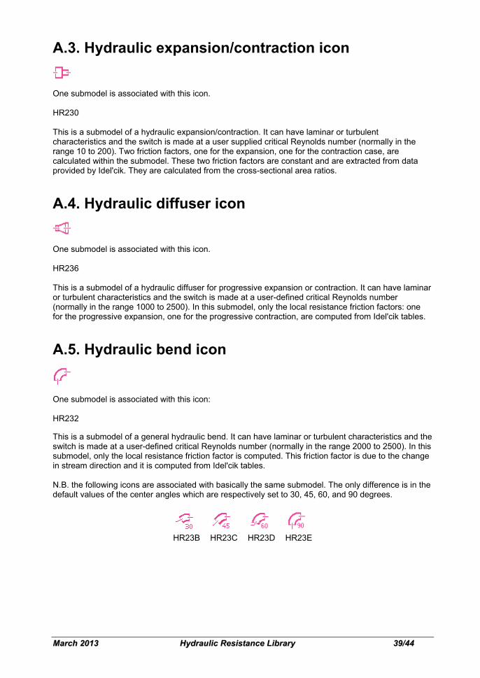
A.3. Hydraulic expansion/contraction icon

One submodel is associated with this icon. HR230 This is a submodel of a hydraulic expansion/contraction. It can have laminar or turbulent characteristics and the switch is made at a user supplied critical Reynolds number (normally in the range 10 to 200). Two friction factors, one for the expansion, one for the contraction case, are calculated within the submodel. These two friction factors are constant and are extracted from data provided by Idel'cik. They are calculated from the cross-sectional area ratios.

A.4. Hydraulic diffuser icon

One submodel is associated with this icon. HR236 This is a submodel of a hydraulic diffuser for progressive expansion or contraction. It can have laminar or turbulent characteristics and the switch is made at a user-defined critical Reynolds number (normally in the range 1000 to 2500). In this submodel, only the local resistance friction factors: one for the progressive expansion, one for the progressive contraction, are computed from Idel'cik tables.

A.5. Hydraulic bend icon

One submodel is associated with this icon: HR232 This is a submodel of a general hydraulic bend. It can have laminar or turbulent characteristics and the switch is made at a user-defined critical Reynolds number (normally in the range 2000 to 2500). In this submodel, only the local resistance friction factor is computed. This friction factor is due to the change in stream direction and it is computed from Idel'cik tables. N.B. the following icons are associated with basically the same submodel. The only difference is in the default values of the center angles which are respectively set to 30, 45, 60, and 90 degrees.

HR23B HR23C HR23D HR23E


A.6 Hydraulic 90 degree T-junction icon

Four submodels are associated with this icon: HR206, HR207, HR260 and HR3P00 HR206 is a submodel of a 3-port T-junction. It can have laminar or turbulent characteristics and the switch is made at a user-defined critical Reynolds number. The user has to supply two constant friction factors. HR207 differs from HR206 in the sense that the pressure at the junction is an implicit variable instead of a state variable. This is the only difference. HR260 use constant Idel’cik friction factors while HR3P00 uses Idel’cik friction factors variable with the Reynolds number. Both allow the user to enter his/her own set of friction factors. N.B. the following icons are associated with basically the same submodel. The difference is in the default values of the friction factors which are set to the values given by Idel'cik for a 45 degree T-junction or for a three port intersecting hole junction.

hrtee45: hrtee90:

HR20B HR20D HR260 HR3P00

HR20C and HR20E

A.7. Hydraulic pipe with centrifugal effects icon

Seven submodels are associated with this icon: HRCE000, HRCE001, HRCE010, HRCE011, HRCE020, HRCE021, HRCE030 These are submodels of hydraulic pipes with centrifugal effects. It is assumed that the rotation axis intersects the axis of the pipe with an angle to be supplied. Compressibility and friction are taken into account. These submodels are used to evaluate the centrifugal effect on pressure drops in a pipe element rotating around an axis which intersects its own axis. 4 different causalities are available: C-R-C : HRCE000, HRCE001 (steady-state) C-R: HRCE010, HRCE011 (steady-state) R-C: HRCE020, HRCE021 (steady-state) R: HRCE030 (steady-state)


A.8. Hydraulic pipe with centrifugal effects and variable rotary speed icon

Seven submodels are associated with this icon: HRCE100, HRCE101, HRCE110, HRCE111, HRCE120, HRCE121, HRCE130 These are submodels of hydraulic pipes with centrifugal effects. The rotary speed is given through the signal port. It is assumed that the rotation axis intersects the axis of the pipe with an angle to be supplied. Compressibility and friction are taken into account. These submodels are used to evaluate the centrifugal effect on pressure drops in a pipe element rotating around an axis which intersects its own axis. 4 different causalities are available: C-R-C : HRCE100, HRCE101 (steady-state) C-R: HRCE110, HRCE111 (steady-state) R-C: HRCE120, HRCE121 (steady-state) R: HRCE130 (steady-state)

A.9. Hydraulic annular pipe icon

One submodel is associated with this icon. HR234 This is a submodel of a hydraulic annular pipe. In annular pipes, the flow is considered to be always laminar. The friction factor is a frictional drag and it is corrected when the eccentricity between the internal and external cylinder is different from 0.

A.10. Hydraulic grooved bushing icon

One submodel is associated with this icon: HRBU01 This is a submodel of a hydraulic grooved bushing. The total flow is evaluated by summing the annular and groove leakage flows to the pumping flow due to the shaft.


A.11. Hydraulic static pressure transducer

Two submodels are associated with this icon: HRPT2, HRPT3 These are complementary submodels. We have seen previously that hydraulic resistance submodels all work with total pressures. Therefore, there was a need to create these two submodels in order to evaluate the static pressures involved in the network. The user has to take great care because to evaluate the static pressure we have to know the cross-sectional area of the pipe where the pressure is measured so as to compute the dynamic pressure and subtract it from the total pressure. Therefore it is recommended to check that the diameter of the pipe where the static pressure is to be calculated is supplied correctly! In appendix B, there is a list of local resistance friction factors given in the literature which are suitable for some submodels described previously.

A.12. Modulated bearings fed by the housing

Three submodels are associated with this icon, depending on the type of bearing (hole, with or without a circumferential groove). Each submodel may take hydrodynamic effects in account. All are assumed to be fed by the bearing housing. HRBEA0010, HRBEA0011, HRBEA0012 These submodels are the corresponding modulated submodels of the submodels HRBEA0010, HRBEA0011 and HRBEA0012. The equations used are consequently the same. The only difference concerns the method of setting the load and the rotary speed (since these variables can be functions of time and/or crankshaft angle) by using signal ports. The user has the choice of describing the load in a polar or rectangular mode.


A.13. Modulated bearings fed by the journal

One submodel is associated with this icon. This submodel may take hydrodynamic effects into account. It is assumed to be fed by the journal. HRBEA0040 These submodels represent bearings with a single oil feed hole. Use HRBEA040 to model a cam bearing, a connecting rod bearing which is fed by the journal.

A.14. Tabulated bearings

HRBEA0020 This submodel makes it possible to compute the volumetric flow rate in the bearing using a 3D look-up table. The three inputs of the table are X, Y and dp, X and Y being inputs at ports 2 and 3 and arbitrarily set by the user. The ports referenced by X and Y can be supplied (for example) with the mep (mean effective pressure), the speed, the load…


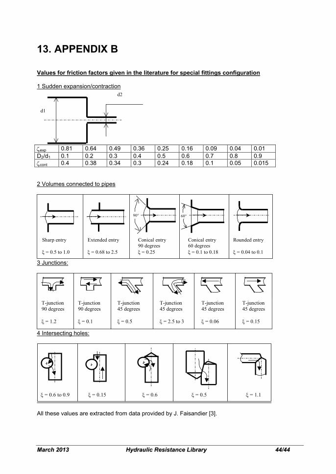
13. APPENDIX B Values for friction factors given in the literature for special fittings configuration 1 Sudden expansion/contraction

d1

d2

ζexp 0.81 0.64 0.49 0.36 0.25 0.16 0.09 0.04 0.01 D2/d1 0.1 0.2 0.3 0.4 0.5 0.6 0.7 0.8 0.9 ζcont 0.4 0.38 0.34 0.3 0.24 0.18 0.1 0.05 0.015 2 Volumes connected to pipes

Sharp entry ξ = 0.5 to 1.0

Extended entry ξ = 0.68 to 2.5

Conical entry 90 degrees ξ = 0.25

Conical entry 60 degrees ξ = 0.1 to 0.18

Rounded entry ξ = 0.04 to 0.1

90° 60°

3 Junctions:

T-junction 90 degrees ξ = 1.2




T-junction 45 degrees ξ = 2.5 to 3


4 Intersecting holes:

ξ = 0.6 to 0.9 ξ = 0.15 ξ = 0.6 ξ = 0.5 ξ = 1.1

All these values are extracted from data provided by J. Faisandier [3].

lms imagine.lab amesim -...

Documents