listening to noise - arxiv · listening to noise david b. kaplan the growth of noise in the...

Listening to Noise

Michael G. EndresTheoretical Research Division, RIKEN Nishina Center, Wako, Saitama 351-0198, JapanE-mail: [email protected]

David B. Kaplan∗

Institute for Nuclear Theory, University of Washington, Seattle, WA 98195-1550, USAE-mail: [email protected]

Jong-Wan LeeInstitute of Particle and Nuclear Studies (IPNS), KEK, 1-1 Oho, Tsukuba, Ibaraki, JapanE-mail: [email protected]

Amy N. NicholsonDeptartment of Physics, University of Maryland, College Park MD 20742-4111, USAE-mail: [email protected]

We show how sign problems in simulations of many-body systems can manifest themselves inthe form of heavy-tailed correlator distributions, similar to what is seen in electron propagationthrough disordered media. We propose an alternative statistical approach for extracting groundstate energies in such systems, illustrating the method with a toy model and with lattice data forunitary fermions.

The XXIX International Symposium on Lattice Field Theory - Lattice 2011July 10-16, 2011Squaw Valley, Lake Tahoe, California

∗Speaker.

c© Copyright owned by the author(s) under the terms of the Creative Commons Attribution-NonCommercial-ShareAlike Licence. http://pos.sissa.it/

arX

iv:1

112.

4023

v1 [

hep-

lat]

17

Dec

201

1

mailto:[email protected]




Listening to Noise David B. Kaplan

1. Introduction

While QCD is accepted as the correct theory of the strong interactions, it is frustrating that westill are unable to derive from it the basic properties of matter or map out a phase diagram that ismore than a cartoon. The problem is that the only tool we have for analyzing QCD nonperturba-tively outside of special kinematic regions is the lattice, and lattice QCD faces daunting barriersto investigating systems with significant baryon number. In the grand canonical formulation, theproblem encountered is that the fermion determinant has a rapidly varying phase leading to strongcancelations in the path integral and a suppression of the partition function that is exponential inthe volume. This is often called the “fermion sign problem", although we will argue it is not spe-cific to fermions. In a canonical formulation, where one computes correlation functions of fixedbaryon number, one encounters a couple of problems. The first is that the measurements may be-come increasingly noisy as the baryon number is increased, which we will call a “noise problem".The second is that the value obtained for the correlator may be relatively quiet, yet drift with time,giving no evidence for a plateau in the effective mass from which one can infer a ground stateenergy. The effective mass computed from a correlator in a system with discrete nonzero energylevels must exhibit a plateau at late time; so if a plateau is absent it follows that the path integralis not being estimated correctly, with little overlap between the field configurations being sampledand the ones that actually dominate in a correct estimation of the correlator. We will refer to thissecond problem as an “overlap problem". In an actual simulation both problems may be foundsimultaneously: a drifting and noisy value for the correlator.

After arguing that the problems encountered in the canonical and grand canonical approachesarise from the same physics, we focus on the canonical method and the statistical distribution ofcorrelators. We give examples where the overlap problem is a manifestation of an underlyingstatistical distribution for the correlator which is very heavy-tailed, and not too far off a log-normaldistribution. We show that the appearance of nearly log-normal distributions is indicative of a meanfield theory expansion, such as that used to study electron properties in disordered media. We thendevelop a technique to effectively overcome the overlap problem by defining mass plots using anestimator which is not minimum bias, but where the log-normal result is the first term in a well-defined expansion. This method has been used with great success in studies of trapped “unitaryfermions" — a strongly coupled nonrelativistic conformal theory relevant to trapped atoms at aFeshbach resonance — allowing a measurement of the ground state energy of up to 70 fermions ina harmonic trap. We also show QCD data from the NPLQCD collaboration that indicates similartechniques might aid in the study of QCD; we expect this to be especially so at larger baryonnumber. This work has been published in Ref. [1].

As a possible direction for future research, our approach suggests a renormalization group ap-proach to the statistical distributions of lattice observables, and a way to analyze such distributionsin a manner analogous to effective field theory, where the nth cumulants of the log of the observableplay the role of higher dimension operators in the effective Lagrangian.

2. Noise and the physical spectrum

We first examine the connections between the noise problem encountered in canonical sim-

2


0 10 20 30 40 50!0.04

!0.02

0.00

0.02

0.04

t!btb tE

excited states

plateau

NOISE

Figure 1: Effective mass plot for nine quarks in the triton channel from NPLQCD [7]; annotation by D.K.

ulations and the phase problem due to the fermion determinant in grand canonical computations,developing a heuristic picture for why a sign/noise/overlap problem arises in the first place.

Grand canonical simulations of lattice QCD at nonzero quark chemical potential involve a pathintegral measure that includes a fermion determinant which is neither real nor positive, leading toan exponentially hard computation [2]. It was noticed long ago [3] that the determinant phaseproblem sets in for quark chemical potential µ ≥ mπ/2, even at zero temperature, which seemspeculiar since nothing physical happens until µ > mN/3, mN being the nucleon mass. A beautifulexplanation for this precocious annoyance was given by Splittorff and Verbaarschott [5] (see also[6] for earlier related ideas): they pointed out that in two flavor QCD with degenerate quarks, thequark determinant phase is exactly what sets apart a simulation at finite isospin chemical potential(µu = −µd = µ) from a simulation at finite quark number (µu = µd = µ). In the former system,pion condensation occurs at µ = mπ/2 leading to a drop in the free energy density, and thereforegrowth of the partition function Z which is exponential in the volume. Therefore a simulation atfinite baryon number with µ ≥ mπ/2 must have the quark determinant phase oscillate wildly tocancel this exponential growth, since there is no pion condensate in this system. The sign problemin QCD is therefore characterized by ∆µ = ζ ≡ (MN/3−mπ/2), the difference between the valuesfor µ where the ground states rearrange themselves in the isospin and baryon number systems.

In a canonical simulation of the A-nucleon state one looks instead at the 3A quark correlatorover Euclidian time τ , CA(τ,U), which is a function of the link fields U for the gluons. For shorttimes, the correlator gets contributions from the many excited states with 3A quarks, but at latertime it should be dominated by the ground state for A nucleons. One typically creates an effectivemass plot of

meff(τ) =−1

∆τln〈CA(τ +∆τ,U)〉/〈CA(τ,U)〉 (2.1)

where the average is over an ensemble of link fields and ∆τ = O(1), chosen to optimize the result.When the correlator is dominated by the ground state, the effective mass should be a constant, theground state energy. Fig. 1 shows an effective mass plot for the case for A = 3 provided by theNPLQCD collaboration clearly exhibiting three types of behavior: strong τ-dependence at shorttimes when excited states contribute, a plateau dominated by the mass of the triton, and degradationinto noise at later time.

3


The growth of noise in the correlator makes it difficult to extract a signal without a lot ofstatistics, and the problem is expected to get worse with increasing baryon number. It would havebeen strange if properties of matter at finite baryon density, which are extremely difficult to computein the grand canonical ensemble, were easy to compute in a canonical simulation — and indeed thisnoise problem exhibited by the correlator at late time is presumably an avatar of the sign problem.This sign/noise problem does not arise simply because of Fermi statistics; for example, constructingcorrelators CA as 3A× 3A Slater determinants of quark propagators accounts for Fermi statisticsand leads to a computational cost from the determinant only scaling as (3A)3, not the exponentialdifficulty seen in the grand canonical computation. Instead, the noise is closely related to thephysical spectrum, as has been quantified by Lepage [4]. For example, in QCD the expectation ofa 3A quark correlator for a nucleus of atomic number A and mass MA is 〈CA〉 ∼ e−MAτ , while thevariance in the sample mean CA can be estimated as

σ2 =

1N

(〈C†

ACA〉−〈C†A〉〈CA〉

)∼ 1

Ne−3Amπ τ (2.2)

for sample size N . Since CA corresponds to 3A quark propagators and C†A to 3A anti-quark prop-

agators, the variance is dominated by the state with 3A pions. Thus the signal to noise ratio scalesas ∼

√N exp(−3Aζ τ), where ζ = (MN/3−mπ/2) is the same parameter we saw characterizing

the sign problem in the grand canonical case. This reasoning is rather simplistic, as the overlapbetween the operators and the nucleon or pion states — which will typically contain volume fac-tors – has not been included. However, Fig. 2 shows evidence from QCD simulations by NPLQCDthat the Lepage argument is qualitatively correct. The noise and sign problems are therefore pre-sumably closely related and determined by the physical spectrum of the theory and should not bethought of as solely a “fermion sign problem"; similar issues can also arise in interacting bosontheories.

In either case the problem arises from the existence of multiparticle states for which the en-ergy/constituent is lower than for the states one wants to study: in QCD, quarks are in some senselighter when they are in a pion than when they are in a nucleon, by the amount ζ . This is a problem

2

mN − 3

2mπ

mN − 3

2mπ

pp

p

Figure 2: A plot of−1/t ln(signal/noise ratio) versus time for p (red) and pp (purple) correlators computedin lattice QCD; horizontal lines give the expected values for these quantities using the Lepage argument.Figure supplied by K. Orginos (NPLQCD), annotation by D.K.

4

Listening to Noise David B. KaplanEffective mass plot with standard technique

0 10 20 30 40 500.0

0.2

0.4

0.6

0.8

1.0

1.2

Τ

meffΤE

Free

40 M configs

23

• Drift upward & No plateau is found

Give up?

Figure 3: The effective mass plot for 46 unitary fermions in a box of size L = 12.

that can occur in bosonic systems as well, and so one should not expect the sign problem to simplybe a fermion problem. Simple bosonic path integrals in the grand canonical approach, such asgauged theories with a φ 4 interaction, manifestly have complex action in Euclidian spacetime anda sign problem.

Applying the Lepage argument for CA(τ,U) to higher moments one sees that all odd momentsare proportional to exp(−MAτ) while even moments are all dominated by pion states1. Thus at verylate time τ , the probability distribution for CA(τ,U) will be almost symmetric, implying a noisysample with small mean. At earlier times, however, we will see that the distribution appears to bevery asymmetric and heavy tailed in both QCD and other theories, and it is this regime we wish toanalyze.

3. Unitary fermions and a Mean Field Description

Nonrelativistic spin half fermions with strong short-range interactions tuned to a conformalfixed point where the phase shift satisfies δ (k) = π/2 for all k are called “unitary fermions". Onecan think of the inter-particle interaction as being described by a square well potential tuned tohave a single bound state with zero binding energy, as one takes the width of the potential tozero. The field theory describing this system is conformal, and interesting to study both for itssimplicity and universality, its challenges for many-body theory, and because it can be realized andstudied experimentally using trapped atoms tuned to a Feshbach resonance [8]. It is also an idealnonperturbative theory for studying fermion sign problems on the lattice, being simpler and fasterto simulate than QCD. At its most basic, the lattice action involves the simplest discretization ofthe Euclidean Lagrangian [9]

ψ†(∂τ −∇

2/2M)ψ− 12 m2

φ2 +φψ

†ψ (3.1)

where φ is a non-propagating auxiliary field with m2 tuned to a critical value, and ψ is a spin 12

fermion with mass M; a more sophisticated action tuned to reduce discretization errors was recentlypresented in [10, 11].

1Thanks to Martin Savage for first pointing this out to us.

5


The ground state for N = (N↑+N↓) unitary fermions can be determined by computing thecorrelator for each background φ field, and then averaging over the ensemble of such fields. Onefinds that when N is large, the correlators rapidly become extremely noisy and drift away from aplateau; see for example Fig. 3 for an effective mass plot for N = 46 unpolarized fermions in abox with periodic boundary conditions of size L = 12. In order to better understand the problemsapparent for τ & 10, it is instructive to plot a histogram of the correlator before averaging overthe φ field. This is shown in Fig. 4, which reveals a distribution for N-body correlators CN(τ,φ)

which is increasingly non-Gaussian at late τ; in fact, Fig. 4 shows that it is ln CN which appears tobe roughly normally distributed, so that CN(τ,φ) is approximately log-normal distributed with anincreasingly large σ and long tail at late time.

A log-normal distribution for the correlator is difficult to reconcile with the Lepage argument.First of all, Lepage assumes that the central limit theorem applies and that the distribution of cor-relators is close to Gaussian and well described by the mean and variance, which is evidently notthe case here. As we will see in a toy model below, the Central Limit Theorem may be irrelevant insuch cases, requiring an exponentially large number of configurations to be applicable. Secondly,the size of the variance for this log-normal distribution cannot be related to the physical spectrum ofthe theory using the Lepage argument. The Lepage argument relates the variance in measurementsof CN to the energy of the lightest state coupling to (CN)

2; there are no anti-particles in this theory,and and so (CN)

2 couples to the ground state of a system N particles each of two different speciesof spin 1/2 unitary fermions 2. However, such a theory in the continuum does not have a finiteenergy ground state, being unstable against condensing into a point-like clump. On the lattice, aground state exists for such a system since there is a maximum density due to Fermi statistics andthe cutoff; this ground state is a lattice artifact, however, and even then may have a vanishinglysmall probability to be created by (CN)

2, in which case the variance might be determined by somemetastable or excited state.

The appearance of a heavy-tailed distribution should not be surprising, however, since having

0 50 100 150 200 250 3000.00

0.01

0.02

0.03

0.04

c

Ρ

Τ=32Τ=16Τ=8Τ=4

-2 0 2 4 6 80.0

0.2

0.4

0.6

0.8

1.0

1.2

logHcL

Ρ

Τ=32Τ=16Τ=8Τ=4

Figure 4: Distribution histograms for c = CN(τ,φ) and ln(c) for N = 4 unitary fermions at several timesτ , taken from Ref. [11]. Curves fitting ln(c) are Gaussian, implying that c is approximately log-normaldistributed, with σ2 increasing with time.

2If CN is the product of N↓ antisymmetrized correlators times N↑ antisymmetrized correlators, then (CN)2 corre-

sponds to a product of four groups of antisymmetrized correlators, and is equivalent to the propagator for two distin-guishable species of spin half fermions.

6


fermions wander through a random φ background is similar to the problem of electrons propa-gating in disordered media, where heavy-tailed distributions are ubiquitous in the vicinity of theAnderson localization transition. For example, it is found that for physical quantities such as thecurrent relaxation time or normalized local density of states, the distribution function P(z) scalesas exp(−Cd lnd z). A particularly simple way to derive these results is to use the optimal fluctuationmethod of Ref. [12], which is a mean field approach. We can adapt these methods to the currentproblem, defining the variable Y = lnCN(τ,φ) and computing its probability distribution P(y) as

P(y) ∝

∫Dφe−Sφ δ (Y (τ,φ)− y) =

∫Dφ

dt2π

e−S (3.2)

where Sφ =∫

d4x m2

2 φ 2 and S = Sφ− it(lnCN(τ,φ)−y). Using the PDS subtraction scheme [13] wehave m2 = Mλ/4π , where the renormalization scale λ is taken to be the physical momentum scalein the problem — in this case λ = kF ≡ (3π2N/V )1/3, N/2 being the number of fermions with asingle spin orientation. We proceed now to evaluate this integral using a mean field expansion; it isnot evident that there is a small parameter to justify this expansion, but the leading order result isilluminating and fits the numerical data well. We expand about φ(x) = φ0, t = t0, and use the factthat for large τ the nth functional derivative of lnCN(τ,φ) with respect to φ(x) equals the the 1-loopFeynman diagram with n insertions of ψ†ψ in the presence of a chemical potential µ = k2

F/(2M).The equations for φ0 and t0 are given by

t0 = −im2φ0

〈n(x)〉c=−i

V m2φ0

N

φ0 = −y− lnZ + τE0(N)

Nτ(3.3)

where E0(N) = 3NEF/5 is the total energy of N free degenerate fermions (N/2 of each spin), andZ is the overlap of the source and sink with the free fermion state. The leading term in the meanfield expansion for P(y) can therefore be expressed as P(y) ∝ exp

[− (y−y)2

2σ2

]with

y = lnZ− τE0(N) , σ2 =

409π

E0(N)τ . (3.4)

This describes a log-normal distribution for the N-fermion propagator CN(τ,φ), with both meanand variance growing in magnitude with time in units of the energy of N free degenerate fermions.In Fig. 5 we plot the quantities − 1

E0

∂y∂τ

and 1E0

∂σ2

∂τas a function of N obtained from correlator

distribution data for unitary fermions at late τ , and find that the gross features of the results arecompatible with the mean field estimates of unity and 40/9π obtained from eq. (3.4).

4. A toy model

It would be useful to devise an algorithm to reliably estimate energies without having to ex-haustively sample the long tail of the correlator distribution, yet without making incorrect assump-tions about the exact functional form of that tail. An approach we suggest here is to exploit thegeneral relationship between stochastic variables X and Y = lnX :

ln〈X〉=∞

∑n=1

κn

n!(4.1)

7


where κn is the nth cumulant of Y . This relation can be proved by noting that the generatingfunction for the κn is lnφY (t) where φY (t) = 〈eYt〉 = 〈X t〉 is the moment generating function forY , and evaluating at t = 1, assumed to be within the radius of convergence. The motivation forinvestigating eq. (4.1) is that if the distribution P(X) were exactly log-normal, the above sumwould end after the second term, as κn>2 would all vanish; therefore by replacing the κn by samplecumulants κn and truncating the sum at n = nmax, one might hope to have a reliable estimator forln〈X〉, provided that the systematic error from truncating eq. (4.1) and the statistical error fromsampling κn can be simultaneously minimized.

Distributions with log-normal-like tails arise naturally in products of stochastic variables. Thepropagator CN(τ,φ) for unitary fermions can be expressed in a transfer matrix formalism as theproduct of τ matrices — one per time hop — each of which is the direct product of N V×V matricesof the form e−K/2(1+gϕ)e−K/2, where K is a constant matrix (the spatial kinetic operator), ϕ is arandom diagonal matrix with O(1) entries corresponding to stochastic φ fields living on the timelinks, and g is a coupling constant (identified with 1/m2 from eq. (3.1)) that has been tuned toa particular critical value that is O(1). Unfortunately, little seems to be known about products ofrandom matrices beyond dimension two [16]. Therefore we analyze instead a toy model where wedefine a “correlator" Cτ as a product of random numbers, and an “energy" E = limτ→∞ Eτ where:

Cτ =τ

∏i=1

(1+gϕi) , Eτ =−1τ

ln〈Cτ〉 (4.2)

where 0 ≤ g ≤ 1 and the ϕi are independent and identically distributed random numbers with auniform distribution on the interval [−1,1]. The exact value for the energy is obviously Eτ = 0since the statistical average of the correlator is 〈Cτ〉= 1. The cumulants of the variable Y = ln(Cτ)

are given by

κ1 = τ

[12 log

(1−g2

)+ tanh−1(g)

g −1],

κn

n!= τ

((−1)n

n −Li1−n

(1+g1−g

)(2tanh−1(g))

n

n!

)

for n≥ 2; for g < 1 one finds that the κn/n! rapidly decrease as n increases.In Fig. 6 we show the results of a simulation where we compute Eτ for g = 1

2 and τ =

1, . . . ,1000. At each value of τ we independently generated an ensemble of values for Cτ of

0 10 20 30 40 50 600.8

1.0

1.2

1.4

1.6

1.8

N

409Π

E0-1

¶Σ2

¶Τ Τ®¥

-E0-1

¶y¶Τ Τ®¥

Figure 5: The quantities − 1E0

∂y∂τ

and 1E0

∂σ2

∂τas a function of N for unitary fermions at late times on a lattice

of size L = 10, compared to mean field prediction (dashed lines).

8


50 250 500 1000

0.005

0.

0.01

Κ2Κ3

Eτ = − 1τ lnCτ

Eτ = − 1τ

12 κ2 + 1

6 κ3

Eτ = − 1

τ

12 κ2

τ

nmax = 2nmax = 3

Figure 6: Simulation of the energy Eτ for the toy model eq. (4.2) with g = 12 . The exact answer is Eτ = 0

(black line); exact values of the expansion eq. (4.1) truncated at order nmax = 2,3 are indicated.

Method E stat. error syst. errorconventional 0.014932 0.002485 –

κn≤2 -0.002159 0.000304 -0.002165κn≤3 -0.000412 0.001618 -0.000324κn≤4 -0.000647 0.008379 0.000050κn≤5 -0.001794 0.037561 3.34×10−6

κn≤6 0.010943 0.147739 −1.22×10−6

Table 1: E determined from 250 blocks of 50,000 configurations each for the model with τ = 1000,g = 1/2.

size N = 50,000. From that ensemble we computed Eτ by (i) using the conventional estimatorEτ = − 1

τlnCτ (blue), which shows a striking systematic error for τ & 50, and statistical noise in-

creasing up to τ ' 500 but decreasing beyond that; (ii) using eq. (4.1) truncated at nmax = 2 usingsample cumulants κn (green), showing a τ-independent systematic error with smaller but slowlygrowing statistical error; (iii) eq. (4.1) truncated at nmax = 3 (red) with a negligible constant sys-tematic error but a larger statistical error. Evidently, one trades systematic error for statistical errorby truncating eq. (4.1) at increasingly large nmax.

Table 1 displays results of a simulation of 1.25×107 φ configurations blocked into 250 blocksof 50,000 each, for the model eq. (4.2) at τ = 1000 and g = 1/2. We give the conventionalestimate Eτ = −1/τ lnCτ and estimates based on the cumulant expansion eq. (4.1) truncated atvarious nmax, where the exact value is E = 0. For each method we give the computed value for E

and the statistical error; for the cumulant expansion we also give the exact systematic error fromtruncating eq. (4.1) at n = nmax using our analytic expressions for κn. These numbers show howthe conventional method gives a wrong answer with deceptively small statistical error. For thecumulant expansion one sees again the trade of systematic error for statistical error with increasingnmax. Table 1 shows the combined error is minimized for nmax = 3, justified by noting that thenmax = 4 result with statistical errors encompasses the nmax = 3 result; we suggest this as a practicalalgorithm for determining where to truncate the cumulant expansion in general.

Leaving the toy model and returning to real simulations of unitary fermions, Fig. 7 shows howthe cumulant expansion works for 50 trapped unitary fermions [11], where truncating the expansion

9


2 3 4 5 6120

125

130

135

140

145

150

nmaxEΩ

0 5 10 15 20 25 30 35100

120

140

160

180

Τ

meffΩ

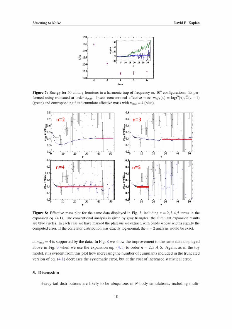
Figure 7: Energy for 50 unitary fermions in a harmonic trap of frequency ω , 106 configurations; fits per-formed using truncated at order nmax. Inset: conventional effective mass me f f (τ) = logC(τ)/C(τ + 1)(green) and corresponding fitted cumulant effective mass with nmax = 4 (blue).

Cumulant expansion method - Results

0 10 20 30 40 500.2

0.3

0.4

0.5

0.6

0.7

0.8

Τ

meff2ΤE

Free

0 10 20 30 40 500.2

0.3

0.4

0.5

0.6

0.7

0.8

Τ

meff3ΤE

Free

0 10 20 30 40 500.2

0.3

0.4

0.5

0.6

0.7

0.8

Τ

meff4ΤE

Free

0 10 20 30 40 500.2

0.3

0.4

0.5

0.6

0.7

0.8

Τ

meff5ΤE

Free

26

n=3


0 10 20 30 40 500.2

0.3

0.4

0.5

0.6

0.7

0.8

Τ

meff2ΤE

Free

0 10 20 30 40 500.2

0.3

0.4

0.5

0.6

0.7

0.8

Τ

meff3ΤE

Free

0 10 20 30 40 500.2

0.3

0.4

0.5

0.6

0.7

0.8

Τ

meff4ΤE

Free

0 10 20 30 40 500.2

0.3

0.4

0.5

0.6

0.7

0.8

Τ

meff5ΤE

Free

26

n=2


0 10 20 30 40 500.2

0.3

0.4

0.5

0.6

0.7

0.8

Τ

meff2ΤE

Free

0 10 20 30 40 500.2

0.3

0.4

0.5

0.6

0.7

0.8

Τ

meff3ΤE

Free

0 10 20 30 40 500.2

0.3

0.4

0.5

0.6

0.7

0.8

Τ

meff4ΤE

Free

0 10 20 30 40 500.2

0.3

0.4

0.5

0.6

0.7

0.8

Τ

meff5ΤE

Free

26

n=4


0 10 20 30 40 500.2

0.3

0.4

0.5

0.6

0.7

0.8

Τ

meff2ΤE

Free

0 10 20 30 40 500.2

0.3

0.4

0.5

0.6

0.7

0.8

Τ

meff3ΤE

Free

0 10 20 30 40 500.2

0.3

0.4

0.5

0.6

0.7

0.8

Τ

meff4ΤE

Free

0 10 20 30 40 500.2

0.3

0.4

0.5

0.6

0.7

0.8

Τ

meff5ΤE

Free

26

n=5

Figure 8: Effective mass plot for the same data displayed in Fig. 3, including n = 2,3,4,5 terms in theexpansion eq. (4.1). The conventional analysis is given by gray triangles; the cumulant expansion resultsare blue circles. In each case we have marked the plateaus we extract, with bands whose widths signify thecomputed error. If the correlator distribution was exactly log-normal, the n = 2 analysis would be exact.

at nmax = 4 is supported by the data. In Fig. 8 we show the improvement to the same data displayedabove in Fig. 3 when we use the expansion eq. (4.1) to order n = 2,3,4,5. Again, as in the toymodel, it is evident from this plot how increasing the number of cumulants included in the truncatedversion of eq. (4.1) decreases the systematic error, but at the cost of increased statistical error.

5. Discussion

Heavy-tail distributions are likely to be ubiquitous in N-body simulations, including multi-

10


t=5

t=10

t=15

t=20

t=25

t=30

t=35

t=40

t=45

-60 -55 -50 -45 -40 -35

0

2000

4000

6000

8000

10 000

12 000

lnHCLLHtL

Figure 9: Statistical distribution of the log of the real part of ΛΛ correlators at different temporal extent tsuggesting a nearly log-normal distribution for the correlators. Each curve represents 100,000 samples; asmall number of correlators with negative real part were discarded. Figure from W. Detmold (NPLQCD).

baryon computations in lattice QCD. An example of the latter is given in Fig. 9, consisting ofhistograms of the log of the ΛΛ correlator, as computed by the NPLQCD collaboration from latticeQCD simulations. This plot shows evidence that the correlator must have a nearly log-normaldistribution during the times considered. Presumably at very late times the distribution of thecorrelator will go over to a Gaussian with large variance and small mean, following the Lepageargument; however, at these earlier times that argument evidently fails, and the types of statisticaltechniques described here and in Ref. [1] might improve the analysis of such QCD data. It isinteresting to speculate whether evidence for log-normal behavior in QCD implies that a meanfield description could be valid for QCD correlators at moderate times, as discussed in §3; note thesimilarity between the QCD example Fig. 9, and the analogous plot for unitary fermions, Fig. 4— as well as the different way the two distributions scale with time. One might expect that ifsuch a mean field description is approximately valid for multibaryon correlators in QCD, as baryonnumber is increased that description would become even more accurate, and log-normal behaviorwould become ubiquitous.

It is also interesting to wonder whether the expansion in eq. (4.1) could be reformulated in aneffective field theory language, where higher cumulants play the role of irrelevant operators. Thereason the correlator distribution is flowing toward a simple universal form (log-normal) is presum-ably because fermions propagating through a single background field configuration are samplingmany values of that field which are nearly statistically independent. What one measures is a sum ofproducts of weakly correlated random matrices. The log of the correlator is in some sense averag-ing over short range fluctuations in the field, and it must be this averaging process — similar to RGblocking — which accounts for the flow of the distribution toward a Gaussian infrared attractor,with deviations characterized by the cumulants of the log of the correlator. Analogies between the

11


RG and statistics are well known — an example being the Central Limit Theorem (see, for example,[14]), or extreme statistics [15]. If the physical basis for attractors for the statistical distribution ofcorrelators was better understood (not much is known about the distributions of products of randommatrices, let alone sums of such products, but see [16]), including a systematic parameterization ofdeviations from the fixed point — analogous to the systematic inclusion of the effects of irrelevantoperators in an effective field theory — then it is conceivable that one could greatly enhance one’sability to find a signal hiding in what superficially looks like useless noise.

Acknowledgments

We are greatly indebted to the NPLQCD collaboration for sharing some of their lattice QCDdata with us, and in particular to W. Detmold and K. Orginos. This work was supported in partby U.S. DOE grant No. DE-FG02-00ER41132. M.G.E is supported by the Foreign PostdoctoralResearcher program at RIKEN.

References

[1] M. G. Endres, D. B. Kaplan, J. -W. Lee and A. N. Nicholson, Noise, sign problems, and statistics,Phys. Rev. Lett. 107, 201601 (2011) [arXiv:1106.0073 [hep-lat]].

[2] M. Troyer and U. -J. Wiese, Computational complexity and fundamental limitations to fermionicquantum Monte Carlo simulations, Phys. Rev. Lett. 94, 170201 (2005) [cond-mat/0408370].

[3] P. E. Gibbs, Understanding finite baryonic density simulations In lattice QCD, PRINT-86-0389(GLASGOW).

[4] G. P Lepage, The analysis of algorithms for lattice field theory, invited lectures given at TASI’89Summer School, Boulder, CO, Jun 4-30, 1989.

[5] K. Splittorff and J. J. M. Verbaarschot, Phase of the fermion determinant at nonzero chemicalpotential, Phys. Rev. Lett. 98, 031601 (2007) [hep-lat/0609076].

[6] T. D. Cohen, QCD functional integrals for systems with nonzero chemical potential, In *Shifman, M.(ed.) et al.: From fields to strings, vol. 1* 101-120 [hep-ph/0405043].

[7] S. R. Beane et al. (NPLQCD collaboration), High statistics analysis using anisotropic clover lattices.II. Three-baryon systems, Phys. Rev. D 80, 074501 (2009) [arXiv:0905.0466 [hep-lat]].

[8] T.-L Ho, Universal thermodynamics of degenerate quantum gases in the unitarity limit, Phys. Rev.Lett. 92, 090402 (2004) [cond-mat/0309109].

[9] J. -W. Chen and D. B. Kaplan, A lattice theory for low-energy fermions at finite chemical potential,Phys. Rev. Lett. 92, 257002 (2004) [hep-lat/0308016].

[10] M. G. Endres, D. B. Kaplan, J. -W. Lee and A. N. Nicholson, A new approach for studying largenumbers of fermions in the unitary regime, PoSLATTICE 2010, 182 (2010) [arXiv:1011.3089[hep-lat]].

[11] M. G. Endres, D. B. Kaplan, J. -W. Lee and A. N. Nicholson, Lattice Monte Carlo calculations forunitary fermions in a harmonic trap, Phys. Rev. A 84, 043644 (2011) [arXiv:1106.5725 [hep-lat]].

[12] I. Smolyarenko and B. Altshuler, Statistics of rare events in disordered conductors, Physical ReviewB 55, 10451 (1997) [cond-mat/9606181].

12


[13] D. B. Kaplan, M. J. Savage and M. B. Wise, A new expansion for nucleon-nucleon interactions, Phys.Lett. B 424, 390 (1998) [nucl-th/9801034].

[14] D. Sornette (2004). Critical phenomena in natural sciences: chaos, fractals, selforganization, anddisorder: concepts and tools, Berlin: Springer.

[15] Györgyi, G. et al., Renormalization-group theory for finite-size scaling in extreme statistics, Phys.Rev. E 81, 041135, (2010)

[16] A. D Jackson et al., Products of random matrices, Phys. Rev. E 66, 066124 (2002) [physics/0202037].

13

listening to noise - arxiv · listening to noise david b. kaplan the growth of noise in the...

Documents