liquidity constraints and the value of insurance …
TRANSCRIPT

NBER WORKING PAPER SERIES
LIQUIDITY CONSTRAINTS AND THE VALUE OF INSURANCE
Keith Marzilli EricsonJustin R. Sydnor
Working Paper 24993http://www.nber.org/papers/w24993
NATIONAL BUREAU OF ECONOMIC RESEARCH1050 Massachusetts Avenue
Cambridge, MA 02138September 2018
We thank Jason Abaluck, Nikhil Agarwal, Jacob Bor, Marika Cabral, Randy Ellis, Amy Finkelstein, Neale Mahoney, Michaela Pagel, Jim Rebitzer, and Jeremy Tobacman for helpful comments, as well as workshop participants at Boston University, the BU-Harvard-MIT Health Seminar, the National Bureau of Economics Summer Institute, the University of Pennsylvania’s Behavioral Economics and Health Symposium, the University of Texas, and the University of Wisconsin, Madison. The views expressed herein are those of the authors and do not necessarily reflect the views of the National Bureau of Economic Research.
NBER working papers are circulated for discussion and comment purposes. They have not been peer-reviewed or been subject to the review by the NBER Board of Directors that accompanies official NBER publications.
© 2018 by Keith Marzilli Ericson and Justin R. Sydnor. All rights reserved. Short sections of text, not to exceed two paragraphs, may be quoted without explicit permission provided that full credit, including © notice, is given to the source.

Liquidity Constraints and the Value of InsuranceKeith Marzilli Ericson and Justin R. SydnorNBER Working Paper No. 24993September 2018JEL No. D01,D15,D81,G22,I13
ABSTRACT
Insurance affects the variability of consumption over time, which is not captured in standard expected utility of wealth models. We develop a consumption-utility model that shows how liquidity constraints and borrowing costs impact the value of insurance. Liquidity constraints generate high insurance demand when premiums are due smoothly, sometimes leading to seemingly dominated choices. Conversely, a risk-averse person may value insurance below its expected value and appear risk loving when premiums are due in a single payment. Moreover, optimal insurance contracts take different forms with liquidity constraints. We show empirical insurance analysis using the standard model can generate misleading counterfactuals and welfare estimates. Finally, we demonstrate the model’s feasibility and importance with an application to evaluating cost-sharing reductions on the health insurance exchanges.
Keith Marzilli EricsonBoston University Questrom School of Business595 Commonwealth AvenueBoston, MA 02215and [email protected]
Justin R. SydnorWisconsin School of Business, ASRMI DepartmentUniversity of Wisconsin at Madison975 University Avenue, Room 5287Madison, WI 53726and [email protected]

Ericson and Sydnor Liquidity Constraints and the Value of Insurance
1
How do we understand the value of insurance? Both foundational theory on insurance demand
(e.g., Arrow 1963; Rothschild and Stiglitz, 1976) and most recent empirical work analyzing
individual insurance decisions (e.g., see Einav, Finkelstein and Levin, 2010) rely on a static
expected-utility model where different levels of insurance equate to different lotteries over
terminal wealth.1 While this framework is a valuable simplification, it abstracts from how
insurance affects the flow of consumption utility over time (Gollier, 2003). How insurance affects
consumption flows is particularly important for those with low levels of liquid financial assets who
face either limits to or high costs for borrowing. There is ample evidence that many households
find themselves facing these types of “liquidity constraints”.2 For example, roughly half of
American households report they would have difficulty paying for an emergency $400 expense
(Federal Reserve, 2015) and nearly half report having liquid assets lower than their health-
insurance deductible (Claxton et al., 2015).
We examine how liquidity constraints affect a rational agent’s willingness to pay for
insurance in a dynamic consumption-utility framework in the absence of moral-hazard concerns.
We begin by exploring the role of liquidity constraints in a simple setting where the individual
faces the possibility of a single loss occurring at some point during the year and has two available
insurance contracts with moderately different levels of coverage in the form of different
deductibles. This basic situation has been used extensively to motivate recent empirical studies of
insurance demand (e.g., Cohen and Einav, 2007; Einav, Finkelstein and Cullen, 2010; Sydnor,
2010; Barshegyan, 2013; Bhargava et al., 2017). After establishing the modeling framework for
this situation, we use calibrated examples to illustrate a number of important insights for insurance
value under liquidity constraints.
In the consumption-utility framework, a rational agent’s willingness to pay for insurance
is strongly affected by the individual’s interest rate and borrowing limits. Importantly, the effect
of liquidity constraints can depend crucially on the relative consumption shock induced by
premium payments versus uninsured losses. In many insurance markets, insurance premiums can
1 Whether utility is defined over total lifetime wealth, liquid financial wealth, or simply over total spending on a particular insurable loss category is an unresolved issue in the literature. Many empirical applications in insurance economics utilize the Constant Absolute Risk Aversion (CARA) utility function, which makes it possible to abstract away from this question within the traditional expected-utility model. We discuss this in more detail in Section 2. 2 Throughout we use the term “liquidity constraints” to refer broadly to situations where individuals with little assets face borrowing limits and/or high costs of borrowing. In our modeling section and results we distinguish between cases with true limits to borrowing versus situations with no borrowing limits but potentially high interest chargers.
Ericson and Sydnor Liquidity Constraints and the Value of Insurance
2
be spread out across smaller periodic payments at little or no additional cost. For example, in
health insurance many workers have premiums deducted from paychecks throughout the year and
many auto and home insurance plans have periodic-payment options. We show that when
premiums are paid smoothly, the value of additional insurance is higher for those facing liquidity
constraints. The intuition is that for a liquidity constrained individual, insurance has both a classic
risk-protection benefit and also an additional financing benefit. Paying higher insurance premiums
via smooth payments can be a more efficient way of financing losses for a person with liquidity
constraints. In contrast, when insurance premiums must be paid in a lump sum up front, the
premium can generate a large consumption shock as well. In those cases, a liquidity constrained
individual may be willing to pay less than the expected value for additional insurance coverage
(see also Casaburi and Willis, forthcoming). Liquidity constraints can generate both strong risk
aversion and also risk-loving behavior in insurance markets.
These results have important implications for research on the efficiency of choice in
insurance markets (Sydnor, 2010; Abaluck and Gruber, 2011; Handel, 2013; Bhargava et al.,
2017). This literature has documented widespread “mistakes” from the perspective of the standard
model of insurance demand, including a) high willingness to pay for modest reductions in risk
(Sydnor, 2010); b) placing different value on premium versus out-of-pocket costs and caring about
contract features like deductibles above-and-beyond their impact on out-of-pocket risk (Abaluck
and Gruber, 2011); and c) even violations of dominance (Handel, 2013; Bhargava et al., 2017).
There is evidence that people are confused about insurance and that confusion contributes to this
behavior (e.g., Johnson et al., 2013; Loewenstein et al., 2013; Handel and Kolstad, 2015; Bhargava
et al., 2017). However, our results also show the behaviors that appear to be clear mistakes may
not be mistakes once liquidity constraints are considered. For example, we show that a rational
liquidity-constrained person can be willing to pay so much for additional coverage that they would
choose plans that appear dominated from the perspective of the traditional static expected-utility
framework. Further, the assumption that only the distributions of total covered versus uncovered
spending matter for insurance demand, which underlies the normative analysis in the Abaluck and
Gruber (2011) approach, does not hold under liquidity constraints.
In our calibrated examples, variation in liquidity constraints has a larger impact on the
value for insurance than does plausible variation in the coefficient of relative risk aversion when
individuals are liquid. This has important implications for research using structural models that

Ericson and Sydnor Liquidity Constraints and the Value of Insurance
3
estimate risk preferences in the standard insurance model from observed contract choices (e.g.,
Cohen and Einav, 2007; Handel 2013; Handel, Hendel and Whinston, 2015). If demand comes
from the consumption-utility model but researchers use the traditional framework, inferences
about risk aversion will be strongly affected by variation in liquidity constraints. While estimates
of risk aversion in the traditional framework may at times be a useful approximation of the
effective risk attitudes generated by consumption-utility maximization, we demonstrate that the
out-of-sample predictions using traditional risk-aversion estimates can be substantially biased.
We also show that liquidity constraints and the consumption-utility model can change the
nature of the optimal insurance contract. A classic result from Arrow (1963) holds that, in the
absence of moral hazard, the optimal contract for a “risk-averting buyer will take the form of 100
per cent coverage above a deductible minimum.” The intuition is that any other contract design
with the same actuarial value will create a mean-preserving spread of uninsured losses compared
to the straight-deductible contract (Gollier and Schlesinger, 1996). However, we show that in the
consumption-utility model a person with liquidity constraints will sometimes prefer a yearly
contract with a lower deductible, coinsurance above the deductible, and a higher maximum-out-
of-pocket limit to a deductible-only contract with the same actuarial value. The reason for this
departure from the classic result is that with liquidity constraints, utility is affected not only by the
total uninsured loss amount but also by the flow of how those losses arrive. In particular, when
multiple losses can occur, straight-deductible plans expose the liquidity-constrained individual to
larger consumption shocks early in the year (i.e., under the deductible). Lowering the deductible
and adding co-insurance raises the size of total possible uninsured losses, but can help the liquidity-
constrained individual smooth consumption shocks over the year. Complex non-linear contracts
that combine deductibles and coinsurance, like we see in health insurance plans, have primarily
been rationalized in prior literature as a compromise between risk protection and incentives to
combat moral hazard (e.g., Zeckhauser, 1970). Our analysis shows, however, that even in the
absence of moral-hazard concerns, liquidity constraints offer another reason that people may prefer
to avoid contracts with large deductibles in favor of other cost-sharing arrangements.
We demonstrate the importance and feasibility of considering liquidity constraints for
policy questions with an application of the consumption-utility framework to health insurance. We
evaluate the dollar value of the Affordable Care Act’s Cost Sharing Reductions (CSRs) for low-

Ericson and Sydnor Liquidity Constraints and the Value of Insurance
4
income individuals purchasing insurance in the health insurance exchanges (a.k.a. marketplaces).3
Individuals eligible for CSRs get subsidized plans with lower cost-sharing requirements (e.g. lower
deductibles and/or maximum out-of-pocket limits). We use claims data from the Truven
Marketscan database for insured working-age adults to simulate patterns of health-spending for a
representative adult over the course of the year. Given those spending patterns, we then estimate
the reduction in premiums (if premiums were paid smoothly) the individual would need in the non-
CSR plan to be indifferent between that and the receiving the additional coverage of the CSR plan.
We find that this value is strongly affected by the level of liquidity constraints. For example,
consider a person with log consumption utility and income around 125% of the federal poverty
limit, who would be eligible for a subsidized “silver tier” plan with 94% actuarial value instead of
the standard 70%. The expected value of that additional coverage would be just over $1,000. If
the person could borrow costlessly, their value for the additional coverage would only slightly
exceed the expected value. However, if that person could only borrow at high costs like those of
payday loans (e.g., 500% APR) they would benefit by around $200 more than the expected value
from receiving the 94% AV plan and if they were unable to borrow at all, the benefit would be
about $400. These results highlight that properly evaluating a policy like the CSR reductions, and
determining whether the welfare gains to the individuals receiving these benefits exceed the social
costs of obtaining those funds, requires an understanding of the degree of liquidity constraints in
the affected population.
Finally, we present new survey evidence that supports the value of understanding liquidity
constraints when assessing the value of insurance. In a sample of respondents with key
demographics targeted to match national distributions, we find a strong correlation between a
stated desire for lower deductibles at extreme costs (e.g., “dominated plans”) and measures of
liquidity constraints even after controlling for income and education.
Our study builds on a long tradition in economics of models of lifecycle consumption-
utility maximization under various forms of liquidity constraints. We contribute more directly to
prior work exploring the links between risk, liquidity constraints and insurance. Jaffe and Malani
(2017) have a closely related and complementary working paper that develops a model where
individuals can finance health shocks either through ex-ante purchases of a full insurance contract
or ex-post with loans. In their model, the availability of loans lowers the value of having insurance.
3 See DeLeire et al. (2017) for an overview and analysis of cost-sharing reductions in private marketplace plans.
Ericson and Sydnor Liquidity Constraints and the Value of Insurance
5
Similarly, Handel, Hendel and Whinston (2015) simulate that the welfare losses from reduced
insurance coverage or reclassification risk are lower when people can borrow and save. In other
closely related work Casaburi and Willis (forthcoming) highlight the point that liquidity-
constrained individuals will have low demand for insurance when premiums are required up-front
and empirically find that take-up of crop-insurance in a developing country is dramatically higher
if premiums are paid at harvest time when farmers have ample liquidity.4 Our results are
consistent with and help to reconcile the seemingly conflicting insights from these papers, as we
see that liquidity can often lower the value of insurance (as in Handel, Hendel and Whinston, 2015;
Jaffe and Malani, 2017) but may actually increase it when premium payments create their own
large liquidity shocks (as in Casaburi and Willis, forthcoming). Our study also provides novel
results relative to these papers related to the possibility of dominance violations and the nature of
optimal insurance contracts. Our work also shares some similarities to Chetty and Szeidl’s (2007)
model of risk preferences under consumption commitments, which highlights how adjustment
costs can raise the effective level of risk aversion because individuals cannot costlessly reallocate
their consumption profiles in the face of shocks. Relative to Chetty and Szeidl (2007), our study
is focused more on the role of borrowing costs and is more closely tied to the standard insurance
modeling framework. Our study also relates to Gollier (1994; 2003), who highlighted that
precautionary savings should substitute for market insurance over the lifecycle and that there
should be low demand for costly market insurance except when people are up against liquidity
constraints. Finally, our exercise evaluating the benefits of ACA cost-sharing reductions has some
parallels to research on assessing the value of unemployment insurance, which has addressed the
importance of accounting for how insurance affects consumption flows (Hansen and Imrohoroglu,
1992; Gruber, 1997; Chetty, 2008).
In our concluding section we discuss future areas for research extending the use of this
consumption-utility approach for studying insurance markets. For example, while we focus here
on insurance value in the absence of moral hazard, we give a few ideas about how the consumption-
utility approach may interact with moral hazard concerns. We also discuss some of the potential
behavioral foundations of liquidity constraints and give some initial thoughts on where better
understanding those micro-foundations may have value for the study of insurance markets.
4 See also Liu and Myers, 2014 for a related dynamic model of microinsurance demand.
Ericson and Sydnor Liquidity Constraints and the Value of Insurance
6
Section 2. Modeling the Ex-ante Value of Insurance
In this section, we compare the demand for insurance under the classic expected-utility-of-wealth
framework and the consumption-utility framework that accounts for liquidity constraints. We
focus on the simplest case where there is only one possible loss 𝐿𝐿 > 0 that will occur during a
given time period with some fixed probability 𝜋𝜋. We assume the individual has background wealth
𝑤𝑤0, which for simplicity we assume is certain except for the possible loss.
The individual can purchase an insurance contract to cover part of this loss. Insurance
contracts are denoted 𝑍𝑍𝑗𝑗, and specify a total premium payment 𝑃𝑃𝑗𝑗 for the policy and a deductible
𝐷𝐷𝑗𝑗 . We assume that the size of the potential loss is greater than the deductible in any policy under
consideration. In the event the loss occurs, an individual who purchased insurance pays the
deductible and is fully insured for the remaining loss above the deductible. Later in the paper we
consider insurance with more complicated cost-sharing designs, but use this simple and standard
case as our starting point.
2.1 Static Expected Utility of Wealth Framework The well-known formulation for expected utility with insurance contract 𝑍𝑍𝑗𝑗 in the static
expected-utility-of-wealth framework is then given by
𝐸𝐸𝐸𝐸�𝑍𝑍𝑗𝑗 , 𝐿𝐿,𝜋𝜋,𝑤𝑤0� = 𝜋𝜋𝜋𝜋�𝑤𝑤0 − 𝑃𝑃𝑗𝑗 − 𝐷𝐷𝑗𝑗� + (1 − 𝜋𝜋)𝜋𝜋�𝑤𝑤0 − 𝑃𝑃𝑗𝑗�,
where 𝜋𝜋 is the utility function over final wealth states with the standard assumptions for risk
aversion that 𝜋𝜋′ > 0, 𝜋𝜋′′ < 0. 5 In this framework, what level of initial wealth is relevant for this
calculation is unclear, and many different assumptions are made in practice (e.g. annual or lifetime
wealth).
5 We use 𝜋𝜋 for the utility function in this subsection to distinguish from the more standard 𝑢𝑢 that we use for the utility function over consumption in the next subsection.

Ericson and Sydnor Liquidity Constraints and the Value of Insurance
7
2.2 Dynamic Consumption Utility Framework In the consumption-utility framework, the individual’s utility is defined over consumption.
We assume standard separable discounted utility with a lifetime of 𝑇𝑇 periods so that total
discounted utility for a given anticipated consumption stream is given by:
𝐸𝐸 = ∑ 𝛿𝛿𝑡𝑡𝑢𝑢(𝑐𝑐𝑡𝑡)𝑇𝑇𝑡𝑡=0 ,
where 0 < 𝛿𝛿 ≤ 1 is the constant exponential discount factor, 𝑐𝑐𝑡𝑡 denotes the level of consumption
in period 𝑡𝑡. The instantaneous consumption-utility function 𝑢𝑢 is continuous and concave, with
𝑢𝑢′ > 0,𝑢𝑢′′ < 0.
In the consumption-utility framework, we must specify more information about the timing
of the potential loss and premium payments, which can often be left unspecified in the classic
expected-utility-of-wealth framework. We continue to consider a single loss 𝐿𝐿 that will occur with
probability 𝜋𝜋 during the course of an insurance policy duration (e.g. one year). That insurance
policy spans 𝑁𝑁 periods (e.g. periods are months, 𝑁𝑁 = 12). Note that we typically expect the
number of periods in a lifetime 𝑇𝑇 to be much greater than 𝑁𝑁. In our baseline model, we let there
be a constant per-period probability of the loss conditional on the loss having not yet occurred:
𝜔𝜔𝑡𝑡 = 1 − (1 − 𝜋𝜋)1𝑁𝑁. Similarly, there is a need to denote the timing of how the total premium
payment 𝑃𝑃𝑗𝑗 for insurance policy 𝑍𝑍𝑗𝑗 are made. In our baseline model we consider a case where the
premiums are due in equal installments 𝑝𝑝𝑗𝑗 across the timeframe of the insurance contract so that
𝑃𝑃𝑗𝑗 = ∑ 𝑝𝑝𝑗𝑗.𝑁𝑁𝑡𝑡=0 Later we consider the case of up-front payments.
In the consumption utility framework, a single wealth measure is replaced instead with a
flow of income, assets and interest rates on borrowing and saving. We assume the individual earns
constant income 𝑦𝑦 each period and denote financial assets at time 𝑡𝑡 as 𝑎𝑎𝑡𝑡. The individual earns
gross interest on positive financial assets of 𝑅𝑅𝑠𝑠 each period or can borrow in the form of negative
assets that incur a gross borrowing interest rate of 𝑅𝑅𝑏𝑏. The limit on debt is defined as a minimum
level of (potentially negative) assets allowed 𝑎𝑎𝑚𝑚𝑚𝑚𝑚𝑚. We let 𝑙𝑙𝑡𝑡 ∈ {0,1} be an indicator function for
whether the loss occurs in period t.
Then, assets evolve by the following equation:
𝑎𝑎𝑡𝑡+1 = 𝑅𝑅𝑠𝑠�𝑎𝑎𝑡𝑡 + 𝑦𝑦 − 𝑝𝑝𝑗𝑗 − 𝑐𝑐𝑡𝑡� − 𝐷𝐷𝑗𝑗𝑙𝑙𝑡𝑡+1 if 𝑎𝑎𝑡𝑡 + 𝑦𝑦 − 𝑝𝑝𝑗𝑗 − 𝑐𝑐𝑡𝑡 ≥ 0,
Ericson and Sydnor Liquidity Constraints and the Value of Insurance
8
𝑎𝑎𝑡𝑡+1 = 𝑅𝑅𝑏𝑏�𝑎𝑎𝑡𝑡 + 𝑦𝑦 − 𝑝𝑝𝑗𝑗 − 𝑐𝑐𝑡𝑡� −𝐷𝐷𝑗𝑗𝑙𝑙𝑡𝑡+1 if 𝑎𝑎𝑡𝑡 + 𝑦𝑦 − 𝑝𝑝𝑗𝑗 − 𝑐𝑐𝑡𝑡 < 0,
subject to the debt-limit constraint that 𝑎𝑎𝑡𝑡 ≥ 𝑎𝑎𝑚𝑚𝑚𝑚𝑚𝑚 ∀ 𝑡𝑡.
The individual chooses consumption each period to maximize the expected discounted
utility flow, subject to the law of motion for assets and the debt limit. We assume that consumption
is chosen after observing the realization of whether or not the loss occurs in that period. We denote
this dynamic programming problem as:
𝑉𝑉𝑡𝑡 �𝑎𝑎𝑡𝑡| max𝜏𝜏∈0,…,𝑡𝑡
{𝑙𝑙𝜏𝜏}� = max𝑐𝑐𝑡𝑡
𝑢𝑢(𝑐𝑐𝑡𝑡) + 𝛿𝛿𝐸𝐸𝑉𝑉𝑡𝑡+1 �𝑎𝑎𝑡𝑡+1| max𝜏𝜏∈0,…,𝑡𝑡+1
{𝑙𝑙𝜏𝜏}�
Where max𝜏𝜏∈0,…,𝑡𝑡
{𝑙𝑙𝜏𝜏} indicates whether the loss has occurred by period t, and the expectation for
period t+1 is over whether the loss occurs in period t+1, since that affects assets in t+1.
This basic framework is flexible and allows us to explore different types of liquidity
constraints. For example, we can consider a case where the individual can save but is not allowed
to borrow by setting 𝑎𝑎𝑚𝑚𝑚𝑚𝑚𝑚 = 0. Setting both 𝑎𝑎𝑚𝑚𝑚𝑚𝑚𝑚 = 0 and 𝑅𝑅𝑠𝑠=0 captures a more extreme case
where the individual consumes based on cash on hand, with no ability to borrow or accumulate
assets.6
2.3 Measuring the value of insurance We denote the value of insurance using a certainty equivalent approach. Specifically, consider an
individual who has access to insurance coverage 𝑍𝑍𝑘𝑘 with total premium 𝑃𝑃𝑘𝑘 and deductible 𝐷𝐷𝑘𝑘. We
are interested in the value of this coverage relative to an alternative policy with less coverage, 𝑍𝑍𝑗𝑗 .
The lower-coverage policy has a higher deductible such that 𝐷𝐷𝑗𝑗 > 𝐷𝐷𝑘𝑘. We denote the value of the
marginal insurance provided by 𝑍𝑍𝑘𝑘 relative to 𝑍𝑍𝑗𝑗 as 𝑋𝑋𝑘𝑘,𝑗𝑗. We define 𝑋𝑋𝑘𝑘,𝑗𝑗 as the reduction in
premium the lower-coverage plan would need to have to make the individual just indifferent
between the two policies. Formally, we solve for 𝑋𝑋𝑘𝑘,𝑗𝑗 in both the expected utility of wealth
6 Obviously the “cash-on-hand” case is an extreme one, but it may be a reasonable approximation for some liquidity constrained individuals who face high implicit taxes on savings due to threat of theft of savings from household members or others or other behavioral patterns that prevent people from saving. We discuss some of those behavioral factors in the concluding section but do not attempt to introduce them into the model here.

Ericson and Sydnor Liquidity Constraints and the Value of Insurance
9
framework and the consumption-utility framework by finding 𝑋𝑋𝑘𝑘,𝑗𝑗 such that the individual would
be indifferent between plans (𝑃𝑃𝑘𝑘,𝐷𝐷𝑘𝑘) and �𝑃𝑃𝑘𝑘 − 𝑋𝑋𝑘𝑘,𝑗𝑗 ,𝐷𝐷𝑗𝑗�.
2.4 Connection between EU(w) and Consumption-utility Frameworks How are the expected-utility-of-wealth and consumption-utility frameworks related? An
indirect utility function for wealth can arise from maximizing behavior in the consumption-utility
framework. One might think of the risk aversion from the curvature of the utility of wealth in the
classic framework as representing a “reduced form” version of the effective risk preferences that
are generated from the consumption-maximization process.
However, the conditions for this to be the case are restrictive. Because the indirect utility
function approach abstracts from the timing of payments and uncertainty within the year, it cannot
easily capture crucial facts about the demand for insurance that arise within the consumption-utility
framework. As such, Section 3 will show a series of predictions made from the consumption-utility
framework than cannot be produced by the expected utility of wealth model.
We first establish conditions under which the consumption utility function 𝑢𝑢 easily maps
into the indirect utility of wealth function 𝜋𝜋. Assume perfect liquidity: no time discounting (𝛿𝛿 =
1), costless borrowing and savings (𝑅𝑅𝑏𝑏 = 𝑅𝑅𝑠𝑠 = 1), and a debt limit in each period set at remaining
lifetime earnings. In this case, if there were no possibility of a loss and no insurance contract
needed, optimal consumption would simply be to consume 𝑦𝑦 in each period. Denote initial wealth
as the sum of lifetime earnings, 𝑤𝑤0 = ∑ 𝑦𝑦𝑇𝑇𝑡𝑡=0 = 𝑇𝑇𝑦𝑦. Then, the indirect utility function over total
wealth is simply 𝜋𝜋(𝑤𝑤0) = 𝑇𝑇𝑢𝑢(𝑦𝑦).
If the only possibility of loss occurred in the initial consumption period, total lifetime
resources for an individual who purchased an insurance contract 𝑍𝑍𝑗𝑗 would simply be 𝑤𝑤0 − 𝑃𝑃𝑗𝑗 in
the case of no loss occurring and 𝑤𝑤0 − 𝑃𝑃𝑗𝑗 − 𝐷𝐷𝑗𝑗 in the case the loss occurs. Since the person could
perfectly smooth consumption over these lifetime resources, we would have that:
𝜋𝜋�𝑤𝑤0 − 𝑃𝑃𝑗𝑗� = 𝑇𝑇𝑢𝑢 �𝑦𝑦 −𝑃𝑃𝑗𝑗𝑇𝑇� and 𝜋𝜋�𝑤𝑤0 − 𝑃𝑃𝑗𝑗 − 𝐷𝐷𝑗𝑗� = 𝑇𝑇𝑢𝑢 �𝑦𝑦 −
𝑃𝑃𝑗𝑗𝑇𝑇−𝐷𝐷𝑗𝑗𝑇𝑇�
Ericson and Sydnor Liquidity Constraints and the Value of Insurance
10
Then, so long 𝑢𝑢() was homothetic7, 𝜋𝜋(𝑤𝑤) = 𝑢𝑢(𝑐𝑐). That is, if curvature over consumption utility
were 𝑢𝑢(𝑐𝑐) = ln (𝑐𝑐), then the indirect utility function over wealth could be given by 𝜋𝜋(𝑤𝑤) =
ln (𝑤𝑤). In this case, the expected-utility-of-wealth formulation is directly related to the
consumption-utility formulation. It is worth noting here that the appropriate measure of initial
wealth when considering the utility of wealth function 𝜋𝜋 as the indirect utility function from
consumption is lifetime earnings.
This equivalence clearly breaks down if the assumptions of “perfect liquidity” are not met.
More subtly, however, even if we assume “perfect liquidity”, the mapping we lay out here only
holds for the case where the possible loss and insurance arise solely in the first period and all
uncertainty is resolved at the time that consumption is chosen. In a more realistic process, where
the possibility of loss arises over multiple periods, there is an additional distortion in the
consumption-utility process. The distortion arises due to the inability to perfectly forecast total
lifetime resources because one does not know for sure if the loss will occur at all. Due to that
uncertainty, it will not generally be possible to perfectly smooth consumption over all periods,
even under “perfect liquidity”, unless one purchases a full-insurance contract.
Section 3. Results The consumption-utility framework makes a number of predictions about the demand for
insurance that distinguish it from the expected utility of wealth model. In this section, we present
key results that emerge from the consumption-utility framework. Throughout, we illustrate and
provide demonstrations of the results using calibrated examples building on the simple model in
the prior section. We begin with two results in which the consumption-utility framework allows
us to consider issues that are beyond the scope of the expected utility of wealth model.
Result 1: The value of insurance is affected by the interest rates and borrowing limits an
individual faces.
Result 2: The value of insurance is affected by the structure of how premiums are paid.
Our first two results from the consumption-utility framework can be illustrated with a set
of simple calibrated examples depicted in Figure 1. For this figure we solve for the marginal value
7 CRRA utility is homothetic, but CARA is not.
Ericson and Sydnor Liquidity Constraints and the Value of Insurance
11
the individual has for a one-year insurance contract with a $500 deductible versus a $1,000
deductible when facing the possibility of a single larger loss (> $1,000) that occurs with 70%
probability. We set the level of the premium for the higher-coverage option at $4,000 here, which
is equivalent to fair insurance for an implied uninsured loss size of a bit over $6,000 and makes
this example very roughly calibrated to the costs of employer-sponsored insurance in the U.S. We
assume that the individual faces this insurance option in the current year and will then live for
another 20 years with full insurance in those later years.8 For these examples, we assume the
individual has no existing assets and earns annual post-tax income of $20,000 each year, which is
around 170% of the individual federal poverty level for 2018. We shut down time preference: the
individual is perfectly patient (𝛿𝛿 = 1) and there is no return on savings (𝑅𝑅𝑠𝑠 = 1). The individual
has log utility over monthly consumption (𝑢𝑢(𝑐𝑐) = ln (𝑐𝑐)), implying a monthly coefficient of
relative risk aversion of one.
Figure 1 will illustrate a series of our results. It shows the value for the $500 of additional
insurance coverage at different levels of borrowing interest rate for two scenarios: a) premium
payments are paid smoothly throughout the year in predictable equal installments and b) premium
payments are due up-front in the first month in a lumpy fashion.
We see that the value of additional insurance is very close to the expected value ($350)
when the person can borrow at zero cost and hence has perfect liquidity from lifetime wealth.
However, for higher interest rates, the value of additional insurance diverges from the expected
value. Liquidity constrained individuals will typically prefer smooth premium payments to all-at-
once premium payments. The solid line shows that when the premiums are paid in a smooth
fashion, an individual facing higher borrowing costs will value the insurance more highly. The
intuition for this result is that the smooth premiums facilitate consumption smoothing in the face
of unpredictable uninsured losses (i.e., deductible payments). Smoothing consumption through
premiums becomes more attractive as borrowing costs rise, since smooth premium payments allow
the person to avoid high borrowing costs. In contrast, if the premiums for insurance are required
all at once (up-front in the first month9), those large premium payments must be financed similarly
8 The assumption of full insurance in later years simplifies the analysis. The value of assets in the current year is naturally affected by assumptions about the nature of risk and insurance exposure in future years. 9 Note that it is not merely the premiums being required up-front that can create source of the divergence. The lumpiness itself can be a problem. For a cash-on-hand consumer, who could not save for the premium, a premium due all at once at the end of the year is just as problematic as a premium due all at once at the beginning of the year.

Ericson and Sydnor Liquidity Constraints and the Value of Insurance
12
to uninsured costs. In that case, for this example the value of additional insurance actually falls as
borrowing costs rise, since it becomes more costly to smooth in response to the premium payments.
Figure 1. Value of Insurance by Borrowing Interest Rate and Timing of Premium Payment
Note: Presents the value of $500 additional insurance in the consumption-utility model ($500 v. $1,000 deductible). Assumes a 70% chance of loss. Expected value = $350. Assumes annual income=$20,000, 𝛿𝛿 = 1, 𝑅𝑅𝑠𝑠 = 1, and 𝑢𝑢(𝑐𝑐) =ln (𝑐𝑐).
The consumption-utility framework can produce values of willingness-to-pay for insurance
that cannot be explained in the simple expected utility of wealth model. For instance, seemingly
risk-seeking behavior can result from risk averse preferences.
Result 3: For an individual with risk averse consumption utility, willingness to pay for
insurance can be below its expected value.
Again, see that in Figure 1, the line for the value of insurance with an up-front premium lies below
the expected value of that insurance. This result may be especially important to consider when
0 10 20 30 40 50 100 200
Interest Rate for Borrowing (APR)
250
300
350
400
450
Val
ue o
f $50
0 A
dditi
onal
Insu
ranc
e
Smooth Premium
Upfront Premium

Ericson and Sydnor Liquidity Constraints and the Value of Insurance
13
economists try to estimate the welfare value of insurance programs. The observed willingness to
pay for insurance may be low for liquidity constrained individuals if premium payments are lumpy
and have to be financed with costly borrowing, but those same individuals may nonetheless receive
large welfare benefits from having insurance if it is either provided to them or can be financed
more efficiently.
Result 3 showed how the consumption-utility framework can produce puzzlingly low
willingness-to-pay for insurance. Result 4 shows that it can also produce puzzlingly high
willingness-to-pay for insurance when premiums are paid smoothly, where willingness-to-pay
actually exceeds the amount of the additional insurance coverage. Such a willingness to pay would
violate dominance from the expected utility of wealth model. However, it can make sense for a
liquidity constrained individual because insurance with smooth premiums facilitates lower-cost
consumption smoothing.
Result 4: Liquidity-constrained individuals can have willingness to pay for insurance that
leads to choices that appear dominated from an expected-utility-of-wealth perspective.
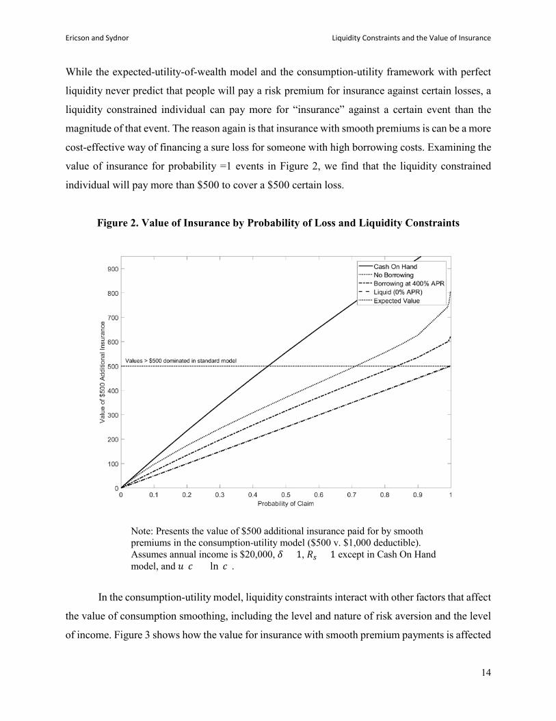
Result 4 can be seen in Figure 2, which replicates the exercise from Figure 1 under the
smooth-premium case but for different probabilities of loss for a few different levels of liquidity
constraints. The horizontal dashed line highlights the dominance-violations where values exceed
$500 (the difference in deductibles for this example). The gap between the individual’s value for
additional insurance and its expected value rises for higher levels of probability, with an especially
strong effect for extreme liquidity constraints. For example, an individual who had “cash-on-hand”
liquidity constraints, such that they could neither borrow nor save, would value lowering the
deductible by $500 at more than $500 if the probability of loss is above 45%. The graph also shows
the “no borrowing” case, where the person cannot borrow but can save, and high borrowing costs
of 400% APR. Both of these cases show similar patterns of generally strong valuation for
additional insurance and violations of dominance for higher levels of probability.
A related additional result can also be seen in Figure 2.
Result 5: Liquidity-constrained individuals can have willingness-to-pay exceeding
expected value for insurance against events that are certain to occur.
Ericson and Sydnor Liquidity Constraints and the Value of Insurance
14
While the expected-utility-of-wealth model and the consumption-utility framework with perfect
liquidity never predict that people will pay a risk premium for insurance against certain losses, a
liquidity constrained individual can pay more for “insurance” against a certain event than the
magnitude of that event. The reason again is that insurance with smooth premiums is can be a more
cost-effective way of financing a sure loss for someone with high borrowing costs. Examining the
value of insurance for probability =1 events in Figure 2, we find that the liquidity constrained
individual will pay more than $500 to cover a $500 certain loss.
Figure 2. Value of Insurance by Probability of Loss and Liquidity Constraints
Note: Presents the value of $500 additional insurance paid for by smooth premiums in the consumption-utility model ($500 v. $1,000 deductible). Assumes annual income is $20,000, 𝛿𝛿 = 1, 𝑅𝑅𝑠𝑠 = 1 except in Cash On Hand model, and 𝑢𝑢(𝑐𝑐) = ln (𝑐𝑐).
In the consumption-utility model, liquidity constraints interact with other factors that affect
the value of consumption smoothing, including the level and nature of risk aversion and the level
of income. Figure 3 shows how the value for insurance with smooth premium payments is affected

Ericson and Sydnor Liquidity Constraints and the Value of Insurance
15
by the borrowing interest rate for different combinations of consumption-utility risk attitudes and
income. The solid black line shows the results for our baseline example where the probability of
loss is 70% and the individual has $20,000 in post-tax yearly income and log monthly consumption
utility (CRRA = 1). The thin line just below that shows how the relationship changes if we hold
fixed the curvature of consumption utility but increase yearly post-tax income to $40,000. Higher
levels of income substantially mute, but do not eliminate, the effects of liquidity constraints on the
value of additional insurance. The thin line above our baseline result shows the effect if we keep
the post-tax yearly income at $20,000 but increase the coefficient of relative risk aversion on
consumption utility from 1 to 2. We see for these cases that increasing the level of risk aversion
makes the value of insurance significantly more sensitive to borrowing costs. Finally, we have also
done this same exercise using constant absolute risk aversion (CARA) utility with the absolute risk
aversion parameter set to match the level of absolute risk aversion for our benchmark case of
CRRA = 1 and income at $20,000. 10 We find that the curve for CARA (not shown) is very
similar to the one for CRRA. As such, CRRA preferences are not driving our results: even though
CARA preferences often avoid the issue of determining the relevant levels of wealth in the
standard model of insurance demand, the value of insurance with CARA preferences are still
sensitive to the interest rate in the consumption-utility framework.
All of these results are consistent with the basic point that the extra value liquidity
constrained people put on additional insurance with smooth premiums is driven by the benefit of
avoiding costly borrowing to engage in consumption smoothing. That force is stronger in situations
where the person would be willing to borrow more despite high borrowing costs (e.g., when
income is low or risk aversion is high).
Result 6: The quantitative effect of liquidity constraints on the value of additional insurance
can be large relative to the effects of income and risk aversion.
Figure 3 also reveals that the quantitative effect of liquidity constraints on the value of
insurance can be quite sizeable when compared with the effects of income and risk aversion. In
particular, we see that for the CRRA utility cases, going from fully liquidity to borrowing costs
10 The available monthly consumption in this case is $1,333.33, which is simply one twelfth of the yearly income after paying the $4,000 baseline premiums. As such, the coefficient of absolute risk aversion for monthly consumption when the coefficient of relative risk aversion is 1 would be a = 1/(1,333.33) = 0.00075.

Ericson and Sydnor Liquidity Constraints and the Value of Insurance
16
around payday-loan level (e.g., 400% APR) increases the value for additional insurance by $50 to
$100 in these examples. In contrast, if borrowing costs are low (e.g., under 10% APR), the income
and risk-aversion variation in these examples affects insurance value by less than $20. This result
relates back to Rabin’s (2000) calibration theorem and the now well-known result that an expected-
utility-of-wealth maximizer should be close to risk neutral over modest stakes, such as additional
insurance on the order of $500. Liquidity constraints, however, can help rationalize strong demand
for insurance over modest stakes.
Figure 3. Effect of Borrowing Costs on Insurance Value by Risk Aversion and Income
Note: Presents the value of $500 additional insurance in the consumption-utility model ($500 v. $1,000 deductible). Assumes a 70% chance of loss, 𝛿𝛿 = 1, and 𝑅𝑅𝑠𝑠 = 1.
Result 7: Inferences about risk aversion using the expected-utility-of-wealth framework
will be strongly affected by variation in liquidity constraints.
0 10 20 30 40 50 100 200 300 400
Interest Rate for Borrowing (APR)
350
360
370
380
390
400
410
420
430
440
450
Val
ue o
f $50
0 A
dditi
onal
Insu
ranc
e
CRRA= 1, Income=$20k
CRRA= 1, Income=$40k
CRRA= 2, Income=$20k
Ericson and Sydnor Liquidity Constraints and the Value of Insurance
17
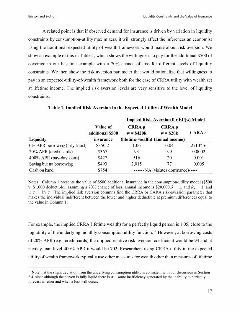
A related point is that if observed demand for insurance is driven by variation in liquidity
constraints by consumption-utility maximizers, it will strongly affect the inferences an economist
using the traditional expected-utility-of-wealth framework would make about risk aversion. We
show an example of this in Table 1, which shows the willingness to pay for the additional $500 of
coverage in our baseline example with a 70% chance of loss for different levels of liquidity
constraints. We then show the risk aversion parameter that would rationalize that willingness to
pay in an expected-utility-of-wealth framework both for the case of CRRA utility with wealth set
at lifetime income. The implied risk aversion levels are very sensitive to the level of liquidity
constraints.
Table 1. Implied Risk Aversion in the Expected Utility of Wealth Model
Notes: Column 1 presents the value of $500 additional insurance in the consumption-utility model ($500 v. $1,000 deductible), assuming a 70% chance of loss, annual income is $20,000,𝛿𝛿 = 1, and 𝑅𝑅𝑠𝑠 = 1, and 𝑢𝑢(𝑐𝑐) = ln (𝑐𝑐). The implied risk aversion columns find the CRRA or CARA risk-aversion parameter that makes the individual indifferent between the lower and higher deductible at premium differences equal to the value in Column 1.
For example, the implied CRRA(lifetime wealth) for a perfectly liquid person is 1.05, close to the
log utility of the underlying monthly consumption utility function.11 However, at borrowing costs
of 20% APR (e.g., credit cards) the implied relative risk aversion coefficient would be 93 and at
payday-loan level 400% APR it would be 702. Researchers using CRRA utility in the expected
utility of wealth framework typically use other measures for wealth other than measures of lifetime
11 Note that the slight deviation from the underlying consumption utility is consistent with our discussion in Section 2.4, since although the person is fully liquid there is still some inefficiency generated by the inability to perfectly forecast whether and when a loss will occur.
Liquidity
Value of additional $500
insurance
CRRA ρ w = $420k
(lifetime wealth)
CRRA ρ w = $20k
(annual income)CARA r
0% APR borrowing (fully liquid) $350.2 1.06 0.04 2x10^-620% APR (credit cards) $367 93 3.5 0.0002400% APR (pay-day loans) $427 516 20 0.001Saving but no borrowing $493 2,015 77 0.005Cash on hand $754
Implied Risk Aversion for EU(w) Model
------NA (violates dominance)-----

Ericson and Sydnor Liquidity Constraints and the Value of Insurance
18
wealth, such as annual income or liquid financial wealth. Table 1 shows the results if we instead
use annual income as the wealth measure. The level of risk aversion is naturally substantially lower
if one assumes annual wealth, but again the risk aversion estimate is strongly affected by liquidity
constraints. This result also highlights that in the full-liquidity case, matching the assumption on
background wealth to lifetime wealth is important for accurately recovering the CRRA risk
attitudes (i.e., log utility) of the consumption utility in the utility-of-wealth function. Finally, the
table also shows the implied estimates of absolute risk aversion if one uses an expected utility of
wealth approach with constant absolute risk aversion (CARA) utility, which is sometimes
attractive because it allows researchers to abstract from issues of wealth effects. Again, however,
the estimates are highly sensitive to underlying liquidity, highlighting that these results are not
unique to CRRA utility and CARA utility does not avoid issues of liquidity constraints affecting
implied risk attitudes.
Result 8: Approximating risk attitudes using the expected utility of wealth framework for
an individual with liquidity constraints can lead to poor out-of-sample predictions.
An important question, however, is whether the expected utility of wealth model can serve
as a reasonable proxy for the risk attitudes generated from the consumption-utility framework for
a person at a given level of liquidity constraints. The expected utility of wealth model will clearly
not be able to capture variation in risk attitudes related to changes in liquidity constraints or the
timing of insurance payments versus uninsured losses that require the consumption-utility
framework. However, can it approximate risk attitudes for a person with fixed liquidity constraints
in similar insurance environments? The expected utility of wealth approximation may be effective
in some cases, but Figure 4 demonstrates that it can lead to poor out-of-sample predictions.

Ericson and Sydnor Liquidity Constraints and the Value of Insurance
19
Figure 4. Out of Sample Predictions from Expected Utility of Wealth for Different Probabilities of Loss
Note: Solid line presents the value of $500 additional insurance in the consumption-utility model ($500 v. $1,000 deductible) for different probabilities of loss (all losses exceed $1,000). Assumes annual income is $20,000, 𝛿𝛿 = 1, 𝑅𝑅𝑠𝑠 = 1, borrowing interest rate at 400% APR, and 20-year life with full insurance after current insurance year. The dashed line presents the implied value for insurance from an expected utility of wealth model with lifetime wealth set at 21*$20,000 = $420,000 and CRRA ρ = 516, which is the risk aversion such that the two models predict the same value for 70% chance of loss.
For this example, we use the baseline example of the value of $500 additional insurance
against a 70% loss to pin down the level of risk aversion implied in the expected utility of wealth
framework. From Table 1 we see that a person who could borrow at 400% APR would be willing
to pay $427 for the lower deductible, which implies a coefficient of relative risk aversion of 516
for a utility of wealth function defined over lifetime wealth. We then plot the value for that same
additional $500 of insurance coverage at different probabilities of loss using both the true
consumption-utility model and the prediction using the implied expected utility of wealth model
(i.e., CRRA for utility of wealth = 516). The expected utility of wealth approximation overstates
0
100
200
300
400
500
600
700
0 0.1 0.2 0.3 0.4 0.5 0.6 0.7 0.8 0.9 1
Valu
e of
Add
ition
al $
500
Insu
ranc
e
probability of loss
EVConsumption utility (400% APR)EU(w) with CRRA ρ=516

Ericson and Sydnor Liquidity Constraints and the Value of Insurance
20
the value of insurance at lower probabilities relative to the true consumption-utility value and
understates it for higher probabilities.12
Section 4. Liquidity Constraints and Optimal Insurance-Contract Design In this section, we demonstrate that liquidity constraints can change the nature of the optimal
design for insurance contracts. Our goal is not to derive general results on the optimal contract
under liquidity constraints, but rather to highlight that the logic for the optimal contract design in
standard insurance models does not hold under liquidity constraints in some important situations.
Arrow (1963) derived a classic result for insurance economics that, in the absence of moral-
hazard concerns, the optimal insurance contract for a risk-averse individual will take the form of
a “straight deductible” with full coverage above the deductible. 13 Gollier and Schlesigner (1996)
demonstrate the strong intuition for the optimality of deductibles by establishing that for the same
level of expected coverage any other contract design will create a mean-preserving spread of
uninsured losses compared to the straight-deductible contract. In the standard model, a straight-
deductible contract will be optimal because it provides the greatest level of risk protection.
Crucially, though, this logic rests on the assumption that utility will be fully determined by the
total amount of uninsured losses and premiums paid for insurance.
A person with liquidity constraints, however, will care not only about the distribution of
total uninsured losses, but also about how those losses arrive. A large loss that arrives all at once
can generate a larger consumption shock than a series of smaller losses that total to the same
amount. As a result, in situations where multiple losses can accrue during the insurance policy
12 As an example where the expected utility of wealth approximation predicts well, we find that it predicts the value for insurance from the consumption-utility framework accurately if we instead hold fixed the probability of loss and just change the size of the additional insurance under consideration (e.g., $1,000 deductible difference). However, we suspect that in more rich examples there will also be effects on the probability of loss. The simple model examples here assume a single possible large loss so that different coverage choices on the margin do not affect the probability of a loss. However, that will not be true more generally. 13 Arrow (1963) writes, “Proposition 1. If an insurance company is willing to offer any insurance policy against loss desired by the buyer at a premium which depends only on the policy's actuarial value, then the policy chosen by a risk-averting buyer will take the form of 100 per cent coverage above a deductible minimum.” Thus, Arrow is not solving the Pareto-optimal (insurer-insuree) contract in this case. Raviv (1979) more systematically identifies cases in which coinsurance would arise. In addition to moral hazard, Raviv (1979) shows that positive coinsurance above the deductible could arise if insurers are risk averse or if the cost of insurance is non-linear in the coverage provided (that is, a load that is not proportional, but convex in the coverage provided).Here, we are examining the optimal policy from the perspective of the consumer, so the issues Raviv raises are not relevant.

Ericson and Sydnor Liquidity Constraints and the Value of Insurance
21
period, such as in health insurance, a person with liquidity constraints might prefer contracts that
reduce the size of most shocks even if they raise the maximum total uninsured loss amount. In
particular, deductibles expose the person to the potential for a large spending shock, especially in
the early parts of the policy period. An alternative with the same expected coverage that lowers
the deductible level will require a higher maximum-out-of-pocket limit but may result in smaller
separate consumption shocks.
We give a simple example to show how the consumption utility model, plus liquidity
constraints, can change the optimal contract design. We consider a baseline straight-deductible
contract, in which the individual is responsible for total losses up to the deductible and then is fully
covered for losses in excess of the deductible. For this example, we set the straight-deductible at
$2,000. We then consider a set of insurance contracts with a “three-arm design” with a deductible,
a coinsurance rate of partial coverage after the deductible up to a maximum-out-of-pocket limit (d,
c, maxOOP). This type of design is relatively common in health insurance, for example. For our
example contracts we fix maxOOP= $2500 in each case, and then for each value of 𝑑𝑑 < $2000,
we solve for the coinsurance rate that delivers the same actuarial value as the straight-deductible
contract (shown in Figure A1). As such, we consider a series of contracts with the same level of
expected coverage and each contract other than the straight-deductible involves a modest increase
in the maximum-out-of-pocket limit.
We examine how the optimal contract from this set of possible contracts depends on the
lumpiness of the risk that the individual faces. We consider two different distributions with the
same probability distribution of total annual claims, but different distributions across months. In
each distribution, the individual faces a ¼ chance each of total annual claims of $30,000, $2000,
$1500, or $0. In the “multiple claims” distribution, annual claims are spread equally out across
months, so the individual will either have 12 months of $2500/month,$167.67/month, $125/month,
or $0/month in claims. In the “single claim” distribution, annual claims are located entirely within
a single month (and each of the 12 months is equally likely to incur the claim). Note that we choose
a distribution with more than 2 outcomes so that coinsurance rates will be relevant and that the
actuarial value will change smoothly with changes in contractual form.14
14 With this distribution the actuarial value for all contracts we consider is 83.6%

Ericson and Sydnor Liquidity Constraints and the Value of Insurance
22
Figure 5. Welfare Effect of Lowering Deductible, Holding Constant Actuarial Value.
Note: Assumes high borrowing costs (𝑅𝑅𝑏𝑏 = 10), annual income is $20,000,𝛿𝛿 = 1, and 𝑅𝑅𝑠𝑠 = 1, and , and 𝑢𝑢(𝑐𝑐) = ln (𝑐𝑐). Welfare effect is measured as the amount of annual income (spread equally across months) the individual would need to be given if they had the $2000 deductible contract to make them indifferent between that contract and the lower deductible contract. In “lumpy claim” distribution, annual claims are located entirely within a single month. In “smooth claims” distribution, annual claims are spread evenly across months.
Figure 5 shows the value a liquidity constrained individual would have for contracts with
different deductible levels under both the “single claim” and “multiple claims” scenarios.15 We
continue with the parameters of our baseline consumption utility model log monthly consumption
15 To make the two cases more easily comparable we make an assumption of “perfect foresight” in the “single claim” scenario. That is, we assume that at the beginning of the policy year the individual learns what loss size he will experience, if any, and the month in which it will occur. With this perfect foresight, the individual can then optimize his consumption path during the year without solving a dynamic consumption problem over the course of the year. This simplifies the programming for our simulation, but also matches the environment in our “multiple claims” case. Our assumption for multiple claims that they arrive smoothly throughout the year implies that the individual learns the loss sequence at the start of the year. We discuss the “perfect foresight” simplification in the next section in more detail, as it has more substance in the context of our application in Section 5.
Ericson and Sydnor Liquidity Constraints and the Value of Insurance
23
utility (i.e., CRRA = 1), and show results with extremely high borrowing costs (900% APR) but
no borrowing limit. This comes close to modeling a cash-on-hand scenario but avoids technical
issues that arise with strict borrowing limits. We see that in the “single claim” example, the classic
Arrow (1963) result holds: the individual prefers the straight-deductible contract to any of the
equivalent-actuarial-value options with lower deductibles. However, in the “multiple claims”
case, the liquidity-constrained individual prefers a contract with a lower deductible but positive
coinsurance coverage. Among these contracts with constant actuarial value, the individual prefers
the contract with deductible just above $1,500 and coinsurance around 3%. Even though lowering
the deductible to this level increases the loss in the worst-case scenario, it increases the expected
welfare for the liquidity-constrained individual by around $100 relative to the Arrow straight-
deductible contract. It is worth noting, however, that liquidity constrained individuals do not
necessarily want the lowest possible deductible level. There remains a tradeoff with risk
protection, and in this case with the individual would prefer the straight-deductible to plans with
deductibles much below $1,500.
5. Application: Valuing Cost-Sharing Reductions
In this section, we apply our consumption-utility framework to a realistic policy case:
valuing the cost-sharing reductions (CSRs) available to people who purchase health insurance on
the health insurance exchanges established by the Affordable Care Act (ACA). This exercise
demonstrates that considering the underlying liquidity constraints of the population affected by
policies affecting insurance markets can have a large effect on estimates of program efficiency.
5.1 Background on CSRs
The ACA introduced CSRs as a way of addressing the affordability of health insurance for
lower-income populations. Insurers who offer health plans on the private health exchanges are
required to offer plan designs with reduced levels of cost sharing (i.e., higher coverage) to lower-
income enrollees who sign up for plans in the ACA silver coverage tier (see DeLeire, Chappel,
Finegold, and Gee 2017 for more on the CSRs). Silver plans must offer 70% actuarial value (AV),
meaning that for a representative population, the insurer pays on average for 70% of the medical

Ericson and Sydnor Liquidity Constraints and the Value of Insurance
24
costs.16 Individuals below 150% of the FPL receive cost-sharing reductions that raise their plan to
an AV of 94%, between 150-200% of FPL have their AV raised to 87% and between 200 and
250% have their AV raised to 73%. Individuals who qualify for a CSR plan receive this higher
level of coverage, but pay the premium level of the original 70% AV silver plan and these
premiums are typically highly subsidized for these individuals.17
Our interest in this section is to estimate within the consumption-utility model how the
value of the additional insurance coverage for an individual receiving a CSR plans would be
affected by that person’s liquidity constraints. For this exercise we compare the value an individual
would have for a CSR plan to a standard 70% AV silver plan using the certainty equivalent
approach outlined in Sections 2 and 3 above. That is, we estimate the reduction in premiums (if
premiums were paid smoothly) the individual would need in the non-CSR plan to be indifferent
between that and the receiving the additional coverage of the CSR plan.
There are many different possible combinations of cost-sharing features (i.e., deductibles,
co-pays, coinsurance) that can be used to achieve the AV targets and ACA enrollees can typically
choose from many different plan designs. For our exercise, we use a set of simple plan designs
that achieve the appropriate AV targets with deductibles and maximum-out-of-pocket limits
similar to those typically seen in the ACA marketplace. Appendix Table A1 gives the details of
the specific plan designs we consider.
5.2 Data and Approach In order to realistically value the insurance provided by the CSRs, we need data on the
distribution of healthcare claims an individual could expect. Importantly, for the consumption-
utility model we need to consider not just the annual level of medical spending for an individual,
but also how those spending needs are distributed over time. We use claims data taken from the
2010 Truven Marketscan database, which provides health care claims for individuals typically
insured by large employers in the U.S. We select individuals age 24-64 continuously enrolled for
16 This AV can be achieved through many different combinations of deductibles, copays, out-of-pocket maximums, etc.—it does not entail a 30% coinsurance rate. 17 The original design of the ACA called for the federal government to compensate insurers for the cost of providing these higher-coverage CSR plans at reduced premiums, though there has been substantial controversy and uncertainty surrounding these federal payments in the subsequent years.
Ericson and Sydnor Liquidity Constraints and the Value of Insurance
25
12 months, and take a 1% sample of them, giving 217,080 enrollees. For each month, we sum the
total inpatient and outpatient spending for that month (including spending originally covered by
insurance and patient cost-sharing). Then, to limit the computational burdens of the exercise, we
select 5,000 individuals at random and use those 5,000 observations as our empirical claims
distribution. As such, our exercise allows for 5,000 distinct claims realizations over the course of
a year from a randomly selected subset of the insured individuals in the Truven Marketscan
database.
To implement the monthly consumption model with this realistic distribution of claims, we
need to specify how individuals’ expectations over future expenses evolve during the year. For
instance, when an individual realizes a certain amount of claims in January, that realization could
change their expectation of claims in future months, which will change their optimal savings and
consumption plans this period. Unfortunately, little is known about individual expectations about
medical expenses (see Ericson, Kircher, Starc, and Spinnewijn 2015 for some results and a
discussion), let alone how they evolve during the year.
As a tractable and conservative approach to this problem, we assume that after individuals
choose their health insurance plan, they learn the complete path of medical expenses they will
incur for the course of the year. That is, in January, the individual will know what their medical
expenses will be in Feb, March,…, December and can plan and save accordingly. Clearly, this
reduces the uncertainty within the year that the individual faces, and is a conservative assumption
that understates the effect of liquidity constraints on the value of insurance. We call this the
“perfect foresight” assumption.18 However, it is important to highlight that while we assume the
individual has perfect foresight over the course of the year about the flow of her medical spending
after selecting insurance, we establish the ex-ante value of insurance before this realization is
known based on the distribution of possible medical-spending needs the individual might face.
18 This assumption also captures, in an ad-hoc way, the idea that individuals may have more time to plan for some bills that others. Here, the individual can begin planning to pay for December medical bills in January—essentially, a 12 month lead time. On the other hand, the individual doesn’t have time to respond to January bills in advance. In truth, bills for some types of services (prescription drugs, elective procedures) are likely due immediately, while others (emergency room visits) can be postponed at some cost.

Ericson and Sydnor Liquidity Constraints and the Value of Insurance
26
Given our perfect foresight assumption, no information is revealed during the year, which
simplifies the analysis since dynamic programming techniques are not necessary. In particular, in
January, individuals can solve the following non-stochastic maximization problem:
max𝑐𝑐1,….,𝑐𝑐12
� 𝛿𝛿𝑡𝑡𝑢𝑢(𝑐𝑐𝑡𝑡) + 𝑉𝑉12(𝑎𝑎13)12
𝑡𝑡=1
subject to borrowing and budget constraints.19 The final term 𝑉𝑉12(𝑎𝑎13) represents the forward
value function at the end of the year given the (possibly negative) assets the individual carries into
the future. For our example, we continue to simplify calculations by assuming that the individual
is fully insured for the remaining lifetime of 20 years after the year under consideration.
5.3. Results
We consider how liquidity constraints affects the value of the CSR plans relative to the
70%-AV silver plan benchmark for an individual with the same income and life horizon as our
examples in Section 3 (e.g., income ~ 125% of the federal poverty line). The true value of the
CSR reductions in the population would naturally be affected by the distribution of assumed
income, liquidity constraints, and assumptions about changing income profiles and lifecycle
horizons. Nonetheless, we think this simple example helps to illustrate how much the welfare
value of this type of public policy can be affected by accounting for liquidity constraints and
provides quantitative estimates that are somewhat realistic.
Table 2 shows the results for an individual with log utility. An individual with perfect
liquidity values additional coverage of the CSR plan at only very slightly more than the expected
value of that coverage. This relates to Rabin’s (2000) point that even a risk averse person will
appear approximately risk neutral over stakes that are modest relative to lifetime wealth, such as
the difference in insurance deductible on the order of around $2,000. However, the value of the
CSRs rises sharply with borrowing costs. For example, an individual who faced borrowing costs
of 500% APR, similar to very costly payday-loan borrowing, values the additional coverage of
going from the 70% AV silver plan to the 73% AV CSR plan at $177, which is 31% higher than
the expected value of that additional coverage. For the 94% AV CSR plan, that same individual
19 We assume annual income = $20,000, annual premiums = $4000, 𝛿𝛿 = 1, and 𝑅𝑅𝑠𝑠 = 1, and , and 𝑢𝑢(𝑐𝑐) = ln (𝑐𝑐).

Ericson and Sydnor Liquidity Constraints and the Value of Insurance
27
would receive a welfare value of $1,236, which is almost $200 more than the expected value for
that additional coverage.
Table 2. Value of Cost-sharing Reductions for CRRA =1 under Liquidity Constraints
Notes: Gives the certainty equivalents that equate the value of the CSR plan to the 70% AV silver plan. See Appendix Table A1 for plan design details. Data source: distributions of monthly health expenditures derived from the 2010 Truven Marketscan claims database. Assumes annual income is $20,000, annual premiums for CSR 70 are $4000, 𝛿𝛿 = 1, and 𝑅𝑅𝑠𝑠 = 1, and , and 𝑢𝑢(𝑐𝑐) = ln (𝑐𝑐).
The additional insurance value for the CSRs implied by the monthly consumption-utility
model for a person with strong liquidity constraints can have important implications for whether
this type of policy is socially beneficial. Providing this type of benefit to low-income people is
often financed by tax revenues, as was the original intention in the ACA for funding the CSRs.
There is, of course, a cost to raising tax revenue due to tax distortions, which affects the marginal
cost of public funds (MCF). The size of the MCF is disputed (see Ballard and Fullerton 1992,
Poterba 1996, and many others.). So for illustration, suppose the MCF were 1.25 (so that each
additional dollar raised in taxes entailed waste of $0.25). Ignoring any gain from redistribution,
we can compare the insurance benefit of the CSRs to the cost of funding them. The social costs of
funding the CSR reductions in this case would be $174 (CSR 73%), $985 (CSR 87%), $1,390
(CSR 94%). The estimates from our model would imply then that the individual welfare value of
the additional coverage is not worth its cost for those who can borrow at credit-card interest rates
and less. However, modest CSRs, such as the 73% CSR could have positive social value for those
whose liquidity situation involves payday borrowing. The 94% CSR reductions would according
to these estimates have positive social value only for those with much stronger liquidity
constraints.
CSR 73% CSR 87% CSR 94%
Expected value of additional coverage $129 $760 $1,042
Value under liquidity constraints Borrow at 0% APR (fully liquid) $129 $760 $1,042 Borrow at 20% APR $137 $800 $1,094 Borrow at 150% APR $171 $888 $1,188 Borrow at 500% APR $177 $934 $1,236
Value of CSR Plan Relative to 70% AV Plan
Ericson and Sydnor Liquidity Constraints and the Value of Insurance
28
Section 6: Survey Evidence on Insurance Value and Liquidity Constraints
We fielded a survey using a Qualtrics panel in November and December of 2015 in order to
investigate the links between liquidity constraints and insurance demand. We recruited 206 adults
between 18 and 65 years old and targeted specific enrollment percentages by gender, age, and
household income in order to get a sample that was similar to the overall U.S. working-age
population on those characteristics.20 Appendix Table A2 gives summary statistics for this sample,
which while not a fully representative U.S. sample has substantial diversity in age, income and
other characteristics.21
For this survey we designed a primary measure of liquidity constraints based on how an
individual would finance an uninsured medical bill. We asked subjects the following question:
“Suppose you had to go to the emergency room because of an accident and just got
a bill from the hospital for $1,000 that is not covered by insurance and is due within
a month. What percent of the $1,000 hospital bill would you cover from each of
these sources (total must add to 100 percent)?”
We asked subjects to consider these sources of funds: “money you already have (e.g.,
savings/checking account); extra money you save by pulling back on spending; extra money you
earn by working more; borrowing from friends/family; borrowing using credit cards or home
equity lines; borrowing using payday or pawn-shop loans; selling things you own; and other
sources.”
20 In order to ensure valid data, we also included two aggressive attention screeners in the survey and only those who passed both of those screeners and who took at least one third of the median time for the survey from a controlled pre-test (11 minutes) were included in the final sample. We contracted with Qualtrics for 200 participants satisfying these screens with balance on the targeted demographics and were delivered 206 respondents. These attention screeners are similar to ones used by Bhargava et al. (2017) in their online surveys about health insurance. They are designed to present a casual reader with a set of options that look like they are asking for an opinion (and hence easy to click without thinking) but the text of the question actually instructs the subject to select a specific option or skip the question completely. Only 32% of Qualtrics panel participants who took the survey passed both of these aggressive attention screeners and are included in the sample. 21 Our sample is better educated than the overall population, with 55% having an associate degree or higher, which is around 10% higher than we would expect from 2015 Census reports. https://www.census.gov/content/dam/Census/library/publications/2016/demo/p20-578.pdf On the other hand, we find that just under 70% of our sample reports private health insurance coverage (employer sponsored and exchange markets) and 11% are uninsured in 2015, which are both close to official statistics for the U.S. population in 2015. See for example: https://www.cdc.gov/nchs/data/nhis/earlyrelease/insur201609.pdf

Ericson and Sydnor Liquidity Constraints and the Value of Insurance
29
We find that only 31% say they would pay the medical bill fully from money they already
have, suggesting that the majority would have to engage in some sort of borrowing or consumption
response to finance the bill. For our analysis in this section, we use the share of the bill the person
says they would pay from existing funds as a simple indicator of liquidity constraints. Specifically,
we find that a median split on this variable occurs at 50% funded from current money, with half
the subjects stating that they would cover 50% or more of the bill from money they already have
and the other half being able to cover less. We label the 50% of the subjects who can cover less
than half of the bill from existing funds as “liquidity constrained”. This measure of liquidity
constraints is, unsurprisingly, strongly but not perfectly correlated with household income. More
than 80% of the respondents reporting household income below $15,000 are liquidity constrained
by this definition. Among the top two income groups, that proportion is significantly lower yet
still substantial at 40%. We also fielded a more traditional question from prior research (Lusardi,
Schneider and Tufano, 2011) that asks people “How confident are you that you could come up
with $2,000 if an unexpected need arose within the next month?” The answers to that question are
highly correlated with our primary measure of liquidity constraints and also match the prior
findings by Lusardi et al.
The survey then asked questions to assess the extent to which people placed value on lower
deductibles and smooth premium payments in ways that would be difficult to reconcile with
frictionless models of consumption smoothing. Two measures related to a willingness to pay for
dominated lower-deductible health plans. We replicated a menu of four hypothetical plan options
from Bhargava et al. (2017) in which three lower-deductible options are dominated by an option
with a $1,000 deductible. The second measure asked subjects to rate which of two arguments they
found more persuasive about the benefits of choosing either a $500 or $1,000 deductible in a
situation where the $1,000 deductible cost $650 less in premium. One argument highlighted that
the high deductible’s premium was so much lower it more than covered the deductible difference
(i.e., dominance argument) and the other highlighted that it might be difficult to set aside money
to pay for higher deductibles (i.e., budgeting argument favoring low deductibles). A final question
asked subjects about their preference for a “rebate plan” motivated by previous work suggesting
this idea in Johnson et al (1993). In this question we asked people to consider either a standard
health insurance plan with a $1,500 annual deductible and an annual premium of $2,000 or an
equivalent “prepay with rebate option”. The rebate plan had a premium that was $1,500 higher for

Ericson and Sydnor Liquidity Constraints and the Value of Insurance
30
the year and no deductible. However, this plan would give a rebate at the end of the year equal to
the difference between $1,500 and their medical spending if their spending came in under $1,500
for the year. See the Appendix for details on these survey questions.
Table 3. Survey Results on Liquidity Constraints and Demand for Insurance
Table 3 presents regression results on the correlation between our indicator for liquidity
constraints and subjects’ answers on these insurance-demand questions. We find a strong positive
correlation between liquidity constraints and a preference for dominated lower deductibles and the
rebate option. Those with liquidity constraints are about 18 percentage points more likely to select
dominated options and to find arguments for doing so persuasive. They are 13 percentage points
more likely to state a preference for a rebate option over a deductible option. We control for both
household income and the respondents’ level of education in these regressions, which suggests
that there may be an important link between liquidity constraints and insurance demand even
beyond income and education effects.
(1) Chose dominated health plan
(2) Find argument for dominated
plan persuasive
(3) Chose and agree w/ dominated
(Combo 1 + 2)
(4) Prefer rebate to
deductibleOverall mean of dependent var: 0.54 0.33 0.27 0.34Liqudity constrained 0.18** 0.17** 0.18*** 0.13*
(0.08) (0.07) (0.07) (0.07)
Control for household income Yes Yes Yes YesControl for level of education Yes Yes Yes YesNumber of observations 206 206 206 206
Measures of desire for insurance to smooth consumption
Notes: Linear regression with heteroscedasticity-robust standard errors in parentheses. *** p < 0.01, ** p < 0.05, * p < 0.10. The independent variable measure for liquidity constraints is an indicator that takes the value of 1 if the subject reported below median fraction of a $1,000 medical bill that they would pay from existing liquid funds (median = 50% paid with liquid funds). The dependent variables are as follows: (1) indicator for selecting a deductible of less than $1,000 in a 4-option hypothetical menu of health plan options with monthly premiums. The 3 lower deductibles all have total premiums that exceed the premiums of the high-deductible option by more than the deductible diffence (i.e., are dominated); (2) Indicator for stating that an argument in favor of choosing one of the lower deductibles from the hypothetical plan choices because of challenges of budgeting for out-of-pocket payments is more persuasive than an alternative argument for the high deductible that highlights dominance, (3) An indicator for both choosing the dominated one and finding the argument for it more persuasive, (4) An indicator for stating a preference for a hypothetical health insurance plan with higher premiums and a rebate at the end of the year over an equivalent plan with a deductible.

Ericson and Sydnor Liquidity Constraints and the Value of Insurance
31
Section 7: Discussion and Conclusion
This paper establishes the importance of accounting for liquidity constraints when assessing the
value of standard insurance contracts. Important insights about insurance emerge from our
consumption-utility model that are not easily captured in standard expected-utility-of-wealth
models. Our survey evidence suggests that there may be value in future empirical work to
collecting measures on individual liquidity constraints when assessing insurance-market
dynamics. Our application to valuing cost-sharing reductions also highlights that normative
evaluations of economic policy related to insurance markets can potentially incorporate
assumptions about borrowing costs and liquidity constraints in a tractable way. Furthermore, our
framework shows that evaluating the benefit of insurance to liquidity-constrained individuals
requires considering how an alternative transfer would be delivered: a lump-sum transfer in liu of
insurance delivers different utility than a transfer delivered smoothly over time. There are,
however, some limitations to our analysis and some important areas for future research to better
understand the links between liquidity constraints and insurance.
One such issue is that in the consumption utility model it matters when bills become due
within the year. A natural question in practical applications is, when are bills actually paid? We
assume here that consumption reductions and borrowing coincide with when bills are generated.
That assumption is likely reasonable for some types of insurance, where cost-sharing must be paid
before the service is rendered. For instance, for both home and auto insurance, contractors and
mechanics typically won’t make repairs without some payment upfront. Yet the timing of
payments is more complicated for some other insurance markets, such as health insurance. Some
medical services require cost-sharing payment in advance of receiving care and likely fit our model
assumptions well. A classic example is prescription drugs, which are typically paid for at the time
the individual acquires the drug. Many physicians’ offices require cost-sharing payment at the time
services are delivered, and this may be more strictly enforced in areas where patients are more
likely to be a payment risk—precisely the liquidity constrained population we are considering. For
many other services, such as emergency room visits and hospitalizations, though, there may be
more flexibility in how quickly bills must be paid. That flexibility creates an additional degree of
freedom for a liquidity-constrained individual. Empirical applications of the consumption-utility

Ericson and Sydnor Liquidity Constraints and the Value of Insurance
32
model for these situations would ideally be paired with more information about the realities of bill
payments and the beliefs people have about their bill-payment options.
Another obvious and important direction for future research is to better understand the link
between liquidity constraints and moral hazard. Our analysis has abstracted from moral hazard to
allow us to isolate important insights about how liquidity constraints interact with the ex-ante value
of risk protection. An analysis of moral hazard is beyond the scope of this paper, but we can
highlight a few initial thoughts on how liquidity constraints may interact with moral hazard.
Liquidity constraints partially explain why individuals respond to the “spot price” of medical care
(the cost sharing they must pay today), not merely their effective end-of-year price (Aron-Dine,
Einav, Finkelstein, and Cullen 2015). We also conjecture that, all else equal, a liquidity constrained
person’s medical utilization will often be more responsive to cost-sharing than a fully liquid
person’s. The reason is that for the same cost-sharing level, the liquidity-constrained person faces
an additional financing or consumption-distortion cost for medical services than a person with
perfect liquidity. As a result, liquidity constraints may provide an explanation for Einav et al.’s
(2013) finding that those whose medical utilization would fall most with higher deductible plans
are least likely to choose them when given an option. It may also be valuable to explore how
liquidity constraints interact with other forms of moral hazard such as how people decide to time
when they incur claims (Cabral, 2017; Diamond et al., 2018).
To the extent that liquidity constraints affect service utilization under insurance, they may
change some of the welfare implications associated with those responses. It may be that increased
utilization when insurance coverage is high represents increased social efficiency if it solves a
liquidity-constraint problem rather than the usual assumption that it represents inefficient waste,
which is similar to arguments in Nyman (1999) and Baicker et al. (2015).
Our consumption utility model highlights new insurance market interventions that may be
useful directions for future research. For instance, part of the demand for insurance when
premiums can be paid smoothly under liquidity constraints comes from the financing benefit of
insurance. Providing improved access to credit may reduce insurance demand in some settings.
As one example, improving access to and awareness of payment plans for medical bills may make
people less averse to high-deductible health plans. There may then be important interactions
between financing opportunities and the extent to which high-deductible plans can be used
effectively to address overutilization of some medical services. As another example, our survey

Ericson and Sydnor Liquidity Constraints and the Value of Insurance
33
provided some evidence that people with liquidity constraints might benefit from slightly altered
insurance arrangements that, for example, substitute rebates for deductibles. More generally
expanding the analysis in this paper to derive the optimal design of insurance contracts under
liquidity constraints and moral hazard would be valuable.
Another important direction for future research in this area is to better understand the links
between liquidity constraints and behavioral biases. In our model of liquidity constraints,
individuals are fully optimizing and make no mistakes. However, a wealth of evidence indicates
that individuals may have incorrect beliefs (e.g. overconfidence) and present-bias or self-control
issues. These behavioral biases could perhaps explain why individuals are so liquidity constrained,
when optimizing models suggest that individuals would strongly benefit from saving or reducing
debt.22 Adding these biases to the consumption-utility model could further enrich the framework,
though would bring additional complexity. It may also be important to better understand how
liquidity constraints interact with confusion about insurance and risk-related biases and heuristics,
such as loss aversion. Our modeling and simulation exercises provide some clear evidence about
how the normative value of insurance should be affected by borrowing costs and debt limits. The
extent to which the consumption-utility model proves useful for positive analysis of observed
demand, however, will likely depend on how liquidity constraints interact with these other
considerations for insurance demand.
Finally, we have limited our analysis to formal liquidity constraints. However, evidence
suggests that people are prone to mental accounting (Thaler 2008), and treat assets as not fungible
across accounts (e.g. Hastings and Shapiro 2013). That is, people may have access to a savings or
retirement account but act as though it were not available to smooth unpredictable shocks, and
thereby reduce consumption rather than assets in response to shocks. Thus, mental accounting and
related heuristics may lead people to act as if they are liquidity constrained, even if they could
smooth consumption (Olafsson and Pagel, forthcoming). A promising direction for future research
is to examine the impact of mental accounting on consumption responses to insurance cost-sharing.
22 Our survey collected a rough measure of present bias based on willingness to delay payments. We find a significant correlation between our measure of liquidity constraints and present bias. However, we see a weaker correlation between the present bias measure and choice of the dominated lower-deductibles for health plans than between our liquidity-constraint measure and dominated choice.
Ericson and Sydnor Liquidity Constraints and the Value of Insurance
34
References Abaluck, Jason and Jonathan Gruber. 2011. “Choice Inconsistencies among the Elderly:
Evidence from Plan Choice in the Medicare Part D Program,” American Economic Review, 101: 1180-1210.
Aron-Dine, A., Einav, L., Finkelstein, A., & Cullen, M. (2015). “Moral Hazard In Health Insurance: Do Dynamic Incentives Matter?” Review of Economics and Statistics, 97(4), 725–741. http://doi.org/10.1162/REST_a_00518
Arrow, Kenneth J. “Uncertainty and the Welfare Economics of Medical Care.” The American Economic Review 53, no. 5 (1963): 941–73.
Baicker, K., Mullainathan, S., and J. Schwartzstein. 2015. “Behavioral Hazard in Health Insurance.” Quarterly Journal of Economics, 130(4): 1623-1667.
Ballard, Charles L., and Don Fullerton. 1992. “Distortionary Taxes and the Provision of Public Goods.” Journal of Economic Perspectives 6 (3): 117–31. doi:10.1257/jep.6.3.117.
Barseghyan, L., F. Molinari, T. O'Donoghue, and J. Teitelbaum. 2013. “The Nature of Risk Preferences: Evidence from Insurance Choices.” American Economic Review 103 (6): 2499-2529.
Bhargava, Saurabh, George Loewenstein, and Justin Sydnor. 2017. “Choose to Lose: Health Plan Choices from a Menu with Dominated Options,” Quarterly Journal of Economics, 132(3): 1319-1372.
Cabral, Marika. 2017. “Claim Timing and Ex Post Adverse Selection,” The Review of Economic Studies, 84(1): 2-44.
Casaburi, Lorenzo, and Jack Willis. Forthcoming. “Time vs. State in Insurance: Experimental Evidence from Contract Farming in Kenya,” American Economic Review.
Chetty, Raj and Adam Szeidl, 2007. "Consumption Commitments and Risk Preferences," The Quarterly Journal of Economics, 122(2), pages 831-877.
Chetty, Raj. 2008. “Moral Hazard vs. Liquidity and Optimal Unemployment Insurance,” Journal of Political Economy, 116(2): 173-234.
Claxton et al. 2015. “Health Benefits In 2015: Stable Trends In The Employer Market.” Health Affairs. 34(10): 1779-1788. doi: 10.1377/hlthaff.2015.0885.
Cohen, Alma and Liran Einav. 2007. “Estimating Risk Preferences from Deductible Choice,” American Economic Review, 97(3): 745-88.
DeLeire, Thomas, Andre Chappel, Kenneth Finegold, and Emily Gee. 2017. “Do Individuals Respond to Cost-Sharing Subsidies in their Selections of Marketplace Health Insurance Plans?”. Journal of Health Economics, 56, pages 71-86.
Diamond, Rebecca, Michael Dickstein, Tim McQuade, and Petra Persson. 2018. “Take-Up, Drop-Out, and Spending in ACA Marketplaces,” National Bureau of Economics Working Paper No 24668.
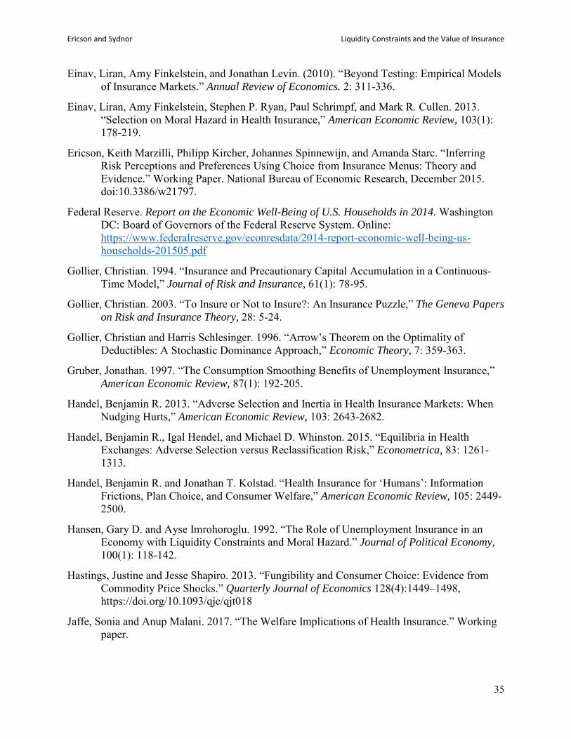
Ericson and Sydnor Liquidity Constraints and the Value of Insurance
35
Einav, Liran, Amy Finkelstein, and Jonathan Levin. (2010). “Beyond Testing: Empirical Models of Insurance Markets.” Annual Review of Economics. 2: 311-336.
Einav, Liran, Amy Finkelstein, Stephen P. Ryan, Paul Schrimpf, and Mark R. Cullen. 2013. “Selection on Moral Hazard in Health Insurance,” American Economic Review, 103(1): 178-219.
Ericson, Keith Marzilli, Philipp Kircher, Johannes Spinnewijn, and Amanda Starc. “Inferring Risk Perceptions and Preferences Using Choice from Insurance Menus: Theory and Evidence.” Working Paper. National Bureau of Economic Research, December 2015. doi:10.3386/w21797.
Federal Reserve. Report on the Economic Well-Being of U.S. Households in 2014. Washington DC: Board of Governors of the Federal Reserve System. Online: https://www.federalreserve.gov/econresdata/2014-report-economic-well-being-us-households-201505.pdf
Gollier, Christian. 1994. “Insurance and Precautionary Capital Accumulation in a Continuous-Time Model,” Journal of Risk and Insurance, 61(1): 78-95.
Gollier, Christian. 2003. “To Insure or Not to Insure?: An Insurance Puzzle,” The Geneva Papers on Risk and Insurance Theory, 28: 5-24.
Gollier, Christian and Harris Schlesinger. 1996. “Arrow’s Theorem on the Optimality of Deductibles: A Stochastic Dominance Approach,” Economic Theory, 7: 359-363.
Gruber, Jonathan. 1997. “The Consumption Smoothing Benefits of Unemployment Insurance,” American Economic Review, 87(1): 192-205.
Handel, Benjamin R. 2013. “Adverse Selection and Inertia in Health Insurance Markets: When Nudging Hurts,” American Economic Review, 103: 2643-2682.
Handel, Benjamin R., Igal Hendel, and Michael D. Whinston. 2015. “Equilibria in Health Exchanges: Adverse Selection versus Reclassification Risk,” Econometrica, 83: 1261-1313.
Handel, Benjamin R. and Jonathan T. Kolstad. “Health Insurance for ‘Humans’: Information Frictions, Plan Choice, and Consumer Welfare,” American Economic Review, 105: 2449-2500.
Hansen, Gary D. and Ayse Imrohoroglu. 1992. “The Role of Unemployment Insurance in an Economy with Liquidity Constraints and Moral Hazard.” Journal of Political Economy, 100(1): 118-142.
Hastings, Justine and Jesse Shapiro. 2013. “Fungibility and Consumer Choice: Evidence from Commodity Price Shocks.” Quarterly Journal of Economics 128(4):1449–1498, https://doi.org/10.1093/qje/qjt018
Jaffe, Sonia and Anup Malani. 2017. “The Welfare Implications of Health Insurance.” Working paper.

Ericson and Sydnor Liquidity Constraints and the Value of Insurance
36
Johnson E., R. Hassin, T. Baker, A. Bajger, and G. Treuer. 2013. “Can Consumers Make Affordable Care Affordable? The Value of Choice Architecture.” PLoS ONE 8(12): e81521. doi:10.1371/journal.pone.0081521.
Johnson, Eric J., John Hershey, Jacqueline Meszaros, and Howard Kunreuther. 1993. “Framing, Probability Distortions, and Insurance Decisions,” Journal of Risk and Uncertainty, 7(1): 35-51.
Liu, Yanyan and Robert J. Myers. 2016. “The Dynamics of Microinsurance Demand in Developing Countries Under Liquidity Constraints and Insurer Default Risk.” Journal of Risk and Insurance, 83(1): 121-138.
Loewenstein, George, Joelle Y. Friedman, Barbara McGill, Sarah Ahmad, Suzanne Linck, Stacey Sinkula, John Beshears, James J. Choi, Jonathan Kolstad, David Laibson, Brigitte C. Madrin, John A. List, and Kevin G. Volpp. 2013. “Consumers’ Misunderstanding of Health Insurance,” Journal of Health Economics, 32: 850-862.
Lusardi, Annamaria, Daniel J. Schneider, and Peter Tufano. 2011. “Financially Fragile Households: Evidence and Implications” Brookings Papers on Economic Activity, 83-134.
Nyman, J.A. 1999. “The Value of Health Insurance: The Access Motive,” Journal of Health Economics 18(2): 141–152.
Olafsson, Arna and Michaela Pagel. Forthcoming. “The Liquid Hand-to-Mouth: Evidence from Personal Finance Management Software.” Review of Financial Studies.
Poterba, James, 1996. Government intervention in the markets for education and health care: how and why? In: Fuchs, Victor (Ed.), Individual and Social Responsibility. University of Chicago Press. Online: http://www.nber.org/chapters/c6566.pdf
Raviv, Artur. 1979. “The Design of an Optimal Insurance Policy.” The American Economic Review 69(1): 84–96.
Rothschild, Michael and Joseph Stiglitz. 1976. “Equilibrium in Competitive Insurance Markets: An Essay on the Economics of Imperfect Information,” Quarterly Journal of Economics, 90(4): 629-649.
Sydnor, Justin. 2010. “(Over)insuring Modest Risks.” American Economic Journal: Applied Economics 2 (4): 177–99.
Thaler, Richard. 2008. “Mental Accounting and Consumer Choice.” Marketing Science: 27(1), pp. 15–25,
Zeckhauser, Richard. 1970. “Medical Insurance: A Case Study of the Tradeoff Between Risk Spreading and Appropriate Incentives,” Journal of Economic Theory, 2(1): 10-
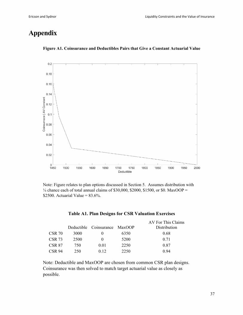
Ericson and Sydnor Liquidity Constraints and the Value of Insurance
37
Appendix
Figure A1. Coinsurance and Deductibles Pairs that Give a Constant Actuarial Value
Note: Figure relates to plan options discussed in Section 5. Assumes distribution with ¼ chance each of total annual claims of $30,000, $2000, $1500, or $0. MaxOOP = $2500. Actuarial Value = 83.6%.
Table A1. Plan Designs for CSR Valuation Exercises
Deductible Coinsurance MaxOOP AV For This Claims
Distribution CSR 70 3000 0 6350 0.68 CSR 73 2500 0 5200 0.71 CSR 87 750 0.01 2250 0.87 CSR 94 250 0.12 2250 0.94
Note: Deductible and MaxOOP are chosen from common CSR plan designs. Coinsurance was then solved to match target actuarial value as closely as possible.

Ericson and Sydnor Liquidity Constraints and the Value of Insurance
38
Appendix A1: Survey details
We fielded a survey using a Qualtrics panel in November and December of 2015 in order
to investigate the links between liquidity constraints, insurance demand and more generally
preferences for smoothing spending shocks through paycheck withdrawals. We contracted with
Qualtrics to provide a 200-person sample and ended up with a final sample of 206 respondents.
We limited the sample to those between 18 and 65 years old. We also targeted specific enrollment
percentages by gender, age, and household income in order to get a sample that was similar to the
overall U.S. working-age population on those characteristics. In order to ensure valid data, we also
included two aggressive attention screeners in the survey and only those who passed both of those
screeners and who took at least one third of the median time for the survey from a controlled pre-
test (11 minutes) were included in the final sample.
Appendix Table A2 gives summary statistics on the self-reported demographic
characteristics of the survey respondents. The balance targeting was successful, as age and
household income breakdowns are close to those reported in the 2013 American Community
Survey. Most importantly, the survey provides a sample with substantial diversity in age, income
and other characteristics. While not a fully representative sample, this gives us increased
confidence that the results from this survey are likely to be more broadly applicable to the U.S.
population. Of course, it is important to remember that the Qualtrics Panels are volunteer panels
and as such the participants are a somewhat selected group even after attempts to obtain balance
on a few target variables. For example, we find that 55% of our sample has an associate degree or
higher, which is around 10% higher than we would expect from 2015 Census reports.23 On the
other hand, we find that just under 70% of our sample reports private health insurance coverage
(employer sponsored and exchange markets) and 11% are uninsured in 2015, which are both close
to to official statistics for the U.S. population in 2015.24
23 See for example: https://www.census.gov/content/dam/Census/library/publications/2016/demo/p20-578.pdf Table 1 reports that the proportion with an associate degree or higher in 2015 was 46.5% for 25 to 34 year olds, 46.7% for 35-44 year olds and 42.6% for 45-64 year olds. 24 See for example: https://www.cdc.gov/nchs/data/nhis/earlyrelease/insur201609.pdf
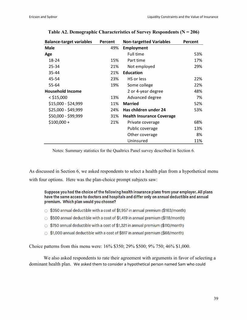
Ericson and Sydnor Liquidity Constraints and the Value of Insurance
39
Table A2. Demographic Characteristics of Survey Respondents (N = 206)
Notes: Summary statistics for the Qualtrics Panel survey described in Section 6.
As discussed in Section 6, we asked respondents to select a health plan from a hypothetical menu
with four options. Here was the plan-choice prompt subjects saw:
Choice patterns from this menu were: 16% $350; 29% $500; 9% 750; 46% $1,000.
We also asked respondents to rate their agreement with arguments in favor of selecting a dominant health plan. We asked them to consider a hypothetical person named Sam who could
Balance-target variables Percent Non-targetted Variables PercentMale 49% EmploymentAge Full time 53%
18-24 15% Part time 17%25-34 21% Not employed 29%35-44 21% Education45-54 23% HS or less 22%55-64 19% Some college 22%
Household Income 2 or 4-year degree 48%< $15,000 13% Advanced degree 7%$15,000 - $24,999 11% Married 52%$25,000 - $49,999 24% Has children under 24 53%$50,000 - $99,999 31% Health Insurance Coverage$100,000 + 21% Private coverage 68%
Public coverage 13%Other coverage 8%Uninsured 11%
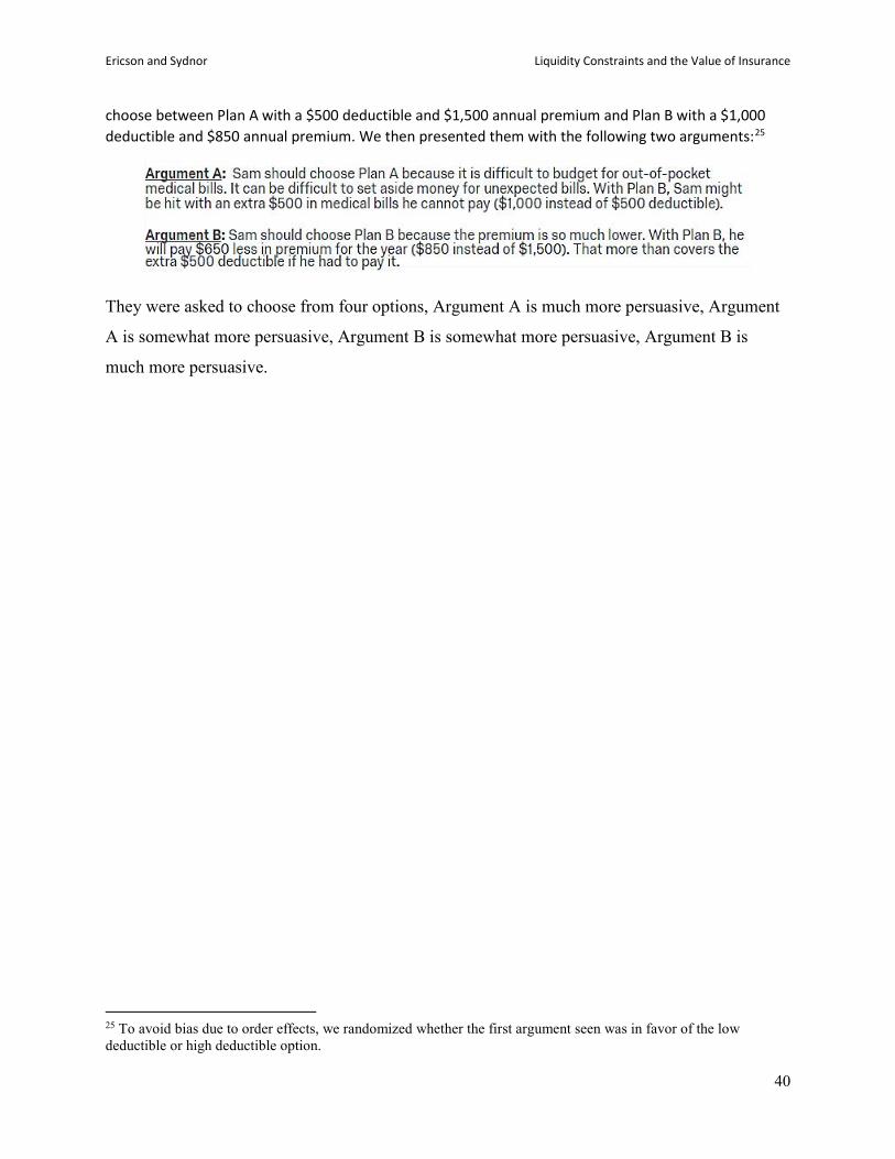
Ericson and Sydnor Liquidity Constraints and the Value of Insurance
40
choose between Plan A with a $500 deductible and $1,500 annual premium and Plan B with a $1,000 deductible and $850 annual premium. We then presented them with the following two arguments:25
They were asked to choose from four options, Argument A is much more persuasive, Argument
A is somewhat more persuasive, Argument B is somewhat more persuasive, Argument B is
much more persuasive.
25 To avoid bias due to order effects, we randomized whether the first argument seen was in favor of the low deductible or high deductible option.