Working Paper 2113 November 2021 Research Department https://doi.org/10.24149/wp2113

Working papers from the Federal Reserve Bank of Dallas are preliminary drafts circulated for professional comment. The views in this paper are those of the authors and do not necessarily reflect the views of the Federal Reserve Bank of Dallas or the Federal Reserve System. Any errors or omissions are the responsibility of the authors.

Bargaining Under Liquidity Constraints: Nash vs. Kalai in the

Laboratory

John Duffy, Lucie Lebeau and Daniela Puzzello

Bargaining Under Liquidity Constraints: Nash vs. Kalai in the Laboratory*

John Duffy†, Lucie Lebeau‡ and Daniela Puzzello§

October 29, 2021

Abstract We report on an experiment in which buyers and sellers engage in semi-structured bargaining in two dimensions: how much of a good the seller will produce and how much money the buyer will offer the seller in exchange. Our aim is to evaluate the empirical relevance of two axiomatic bargaining solutions, the generalized Nash bargaining solution and Kalai's proportional bargaining solution. These bargaining solutions predict different outcomes when buyers are constrained in their money holdings. We first use the case when the buyer is not liquidity constrained to estimate the bargaining power parameter, which we find to be equal to 1/2. Then, imposing liquidity constraints on buyers, we find strong evidence in support of the Kalai proportional solution and against the generalized Nash solution. Our findings have policy implications, e.g., for the welfare cost of inflation in search-theoretic models of money. JEL Codes: C78, C92, D83. Keywords: Bargaining, Monetary Economics, Experimental Economics.

*We gratefully acknowledge funding for this project from the National Science Foundation under grants SES#1529272 and SES#1530820. The experimental protocol used to collect data for this study was approved by the UC Irvine Institutional Review Board, HS# 2015-2082. The views expressed in this paper are those of the authors and are not necessarily reflective of views at the Federal Reserve Bank of Dallas or the Federal Reserve System. †John Duffy, Department of Economics, University of California, Irvine (duffy@uci.edu) ‡Lucie Lebeau, Federal Reserve Bank of Dallas (lucie.lebeau@dal.frb.org) §Daniela Puzzello, Department of Economics, Indiana University, Bloomington (dpuzzell@indiana.edu)

1 Introduction

An important question in economics is how self-interested players bargain in order to achieve

mutually beneficial outcomes. Indeed, there already exists a large experimental literature ex-

ploring various theories of non-cooperative bargaining behavior. For surveys, see e.g., Roth

(1995), Camerer (2003) and Guth and Kocher (2014). A typical bargaining experiment in-

volves a fixed pie, an explicit extensive form for the bargaining process and the absence of any

liquidity constraints.

By contrast, in this paper we study bargaining solutions in settings where the pie size

is determined endogenously and simultaneously with the division of the pie, and bargaining

is only semi-structured. Such settings are commonly used in the labor, money and finance

search, and marketing literatures (see e.g., Lagos and Wright (2005), Aruoba et al. (2007),

Weill (2020) or Iyer and Villas-Boas (2003)) but have not, to our knowledge, been studied

in the laboratory. We further explore the role played by liquidity constraints which create

asymmetries in the bargaining sets between the two players and enable us to distinguish

between two axiomatic solutions as applied to the bargaining problem that we study.1

Indeed, the main contribution of our paper is that we consider the empirical relevance of

two bargaining solutions that have been applied to the two-dimensional bargaining problem

that we study. The first solution is the generalized Nash bargaining solution (Nash (1950),

Nash (1953)) and the second is Kalai’s proportional solution (Kalai (1977)). We focus on

these two axiomatic solutions as they are the most widely used in applied work, and they

can result in different predictions in the two-dimensional bargaining problem that we consider

here, depending on whether or not the liquidity constraints are binding. The novelty of our

approach comes from varying the liquidity constraints that buyers face, that is, the amount

of money the buyer brings to the bargaining game. By varying whether or not buyers face

liquidity constraints, and the restrictiveness of those constraints, we are able to tease apart

distinctions between the Nash and Kalai bargaining solutions so as to clearly identify which

solution better characterizes the data from our experiment.

Nash’s bargaining solution follows uniquely from several axioms: solutions are assumed to

1Liquidity constraints are also empirically relevant; For instance, Gross and Souleles (2002) estimate the

share of potentially liquidity constrained households in the U.S. to be over 66%.

1

be individually rational, Pareto efficient, independent of irrelevant alternatives and invariant to

scale changes in utility representations. By contrast, Kalai’s approach replaces the last axiom,

invariance to scale transformations of utility, with a strong monotonicity axiom, which implies

that the resulting solution exhibits proportionality ; if there are higher gains from trade, then

both parties must gain from that expansion proportionally. A third solution possibility, due

to Kalai and Smorodinsky (1975) replaces the independence of irrelevant alternatives axiom

of Nash with a weaker version of Kalai’s monotonicity axiom. As the applied literature mainly

uses the Nash or Kalai solutions and since the Kalai-Smorodinsky solution responds similarly

to the Nash solution as liquidity constraints are varied, we chose to focus our attention on a

comparison between the Nash and Kalai solutions only.

Relative to the existing literature, we consider an environment that differs in two important

aspects. First, the payoff functions of the buyer and seller are nonlinear and as already noted,

there are two dimensions to the bargaining problem, over quantities and money. Second, we

consider the case where buyers may be liquidity constrained.

We show that in the case where buyers are not liquidity constrained, the Nash and Kalai

approaches yield the same solution. However, in the case where buyers are liquidity constrained

and the payoff functions are nonlinear, we show that the Nash solution will generally differ from

the Kalai solution, enabling a direct test as to which bargaining solution best characterizes

the experimental data.

An alternative approach to the one we pursue here would be to directly test the axioms

that Nash and Kalai rely upon to determine the bargaining solution. However, as we can

directly observe trading behavior in our experiment, it seems less interesting to evaluate more

general axioms, e.g., Pareto optimality, than to consider the relevance of different bargaining

solutions for predicting exchange outcomes. Further, to test the axioms that underlie the two

different bargaining solutions would require testing of different sets of axioms for each solution

that need not overlap. Such an exercise has been attempted by Nydegger and Owen (1974)

who find support for some (but not all) of the axioms found in Nash (1950) and for some

(but not all) of the different axioms found in Kalai and Smorodinsky (1975). More recently,

Navarro and Veszteg (2020) confirm that one axiom assumed in the Nash (1950) and Kalai

and Smorodinsky (1975) solutions – scale invariance – finds little support in their experimental

unstructured bargaining experiments.

2

Our experiment consists of three treatments. In the first treatment, buyers and sellers are

unconstrained in their ability to achieve the first best allocation. In the other two treatments,

buyers are constrained by their money endowments from implementing the first best allocation.

The first, unconstrained treatment, enables us to estimate the distribution of bargaining power

between the buyer and the seller. Given these bargaining weights, the two bargaining solutions

predict different allocations in the two constrained treatments.

To preview our results, in the unconstrained case we estimate that the bargaining weight

is equal to 1/2. Using that bargaining weight we compare the predictions of the Nash and

Kalai bargaining solutions in the constrained case and we find strong evidence favoring the

Kalai proportional solution. Finally, we discuss the implications of our findings for applied

work. Specifically, we show that our estimates have important quantitative implications for

the welfare costs of inflation in search-theoretic models of money.

2 Related Literature

As Karagozoglu (2019) notes, prior to 1982, the experimental literature on bargaining generally

employed unstructured designs. For example, Nydegger and Owen (1974) study two-player

unstructured, face-to-face bargaining over chips where they vary the utility of value of chips

between players and introduce irrelevant constraints to test the axioms of Nash and Kalai

and Smorodinsky. Roth and Malouf (1979) and Roth and Murnighan (1982) study the role

of complete versus partial information about an opponent’s payoffs for outcomes under un-

structured bargaining. Hoffman and Spitzer (1982) and Hoffman and Spitzer (1985) study

unstructured face-to-face bargaining by two or more players in settings where one player has

unilateral power to implement a particular bargaining outcome.

The year 1982 marks an important turning point toward more structured bargaining exper-

iments with the introduction of Rubinstein’s alternating offers bargaining model (Rubinstein

(1982)) and Guth et al.’s ultimatum game (Guth et al. (1982)) both of which have explicit

extensive forms. Subsequently, much research has been conducted using these structured mod-

els of bargaining albeit mainly in the one-dimensional, split a pie framework. For instance

Binmore et al. (1989), Binmore et al. (1998) looked at the role played by outside options and

compared a “split the surplus” solution with a “deal-me-out” solution. In the former solution,

3

both players get their outside option and split equally the remaining pie net of those outside

option values. In deal-me-out, the players agree to split the pie in half unless one player is

worse off than under her outside option, in which case she gets her outside option and the

other player gets the remainder of the pie. The evidence here seems to be more consistent with

the deal-me-out solution.2 Li and Houser (2020) provide a laboratory test of the complete

information stochastic bargaining framework of Merlo and Wilson (1995) where the cake size

and the identity of the proposer follow a stochastic process. Their evidence does not provide

support for the stationary subgame perfect equilibrium prediction. Rather, subjects tend to

agree on proposals associated with the largest equal splits.

More recently there has been a revival of interest in unstructured bargaining experiments.

For instance, Feltovich and Swierzbinski (2011), Anbarci and Feltovich (2013) and Anbarci and

Feltovich (2018) study the role of outside options and disagreement values in one dimensional,

unstructured bargaining games as well as in structured games, such as the Nash demand

game (Nash (1953)). While outside options have to be forgone if parties enter into bargaining,

disagreement values are payoffs earned in the event that a bargain is not reached. They too

find that disagreement values do not matter as much as theory would predict, with subjects

often dividing the pie down the middle regardless of the disagreement values.

Bolton and Karagozoglu (2016) study the role of hard leverage (ultimatum game proposal

rights) versus soft leverage (appeal to a focal precedent) for outcomes in an unstructured

bargaining game and find that focal precedents play an important role in bargaining outcomes.

Dufwenberg et al. (2017) consider unstructured pre-play negotiation in a “lost wallet game”

and vary whether agreed-upon bargaining outcomes are binding or informal (reneging is al-

lowed). They find that regardless of whether negotiated outcomes are binding or informal,

equal splits are the most commonly agreed upon outcome.

Like us, Galeotti et al. (2019) use an unstructured bargaining setting to explore equity-

efficiency trade-offs. However, in their study the bargaining process is over two or three pre-

2Our game, described in Section 3, does not allow us to distinguish between the deal-me-out solution and

the split the surplus solution. Both coincide because outside options are normalized to zero, as is usual in the

search-theoretic literature that makes use of bargaining. In this setup, both of these solutions, when Pareto

efficient, also coincide with the Kalai proportional solution in the special case where the bargaining weights are

symmetric, so that focusing on Kalai bargaining is without loss of generality in our context.

4

defined allocations where an equal split allocation may or may not be efficient and bargaining

only involves online chat between the two parties as to which pre-defined allocation they will

agree upon. Using this design, they find evidence inconsistent with both the Nash (1950) and

Kalai and Smorodinsky (1975) solutions, but they do not address the Kalai (1977) proportional

solution as we do in this paper. Further, they show that focality on equal earnings outcomes is

not universal. Indeed, in decision settings where, unlike in fixed-pie settings, there are trade-

offs between equality and efficiency, a substantial proportion of subjects choose an unequal

and total welfare maximizing allocation over equal and Pareto efficient ones.

Camerer et al. (2019) study unstructured bargaining with one-sided private information.

They find that the incidence of bargaining failures is decreasing in the pie size. They use a

machine learning approach to show that features of the bargaining process play an important

role in the determination of agreements.

Korenock and Munro (2021) study unstructured wage bargaining between firms and work-

ers in a dynamic labor-search model under the assumption that the exogenously determined

match surplus is split equally. They find no effects on wages from changes in the unemployment

rate and an under-reaction of wages to changes in unemployment benefits.

As noted earlier, Navarro and Veszteg (2020) construct unstructured bargaining situations

with the goal of testing the axioms of several bargaining solutions. They provide evidence

against the scale invariance axiom, and show that the Nash bargaining solution and the Kalai-

Smorodinsky solution are poor predictors of bargaining outcomes.

In all of these unstructured bargaining studies, there is typically only a time limit to

bargaining and bargaining typically takes place in a single dimension, e.g., how to divide

a pie. By contrast, we study unstructured bargaining in a two-dimensional setting where

subjects simultaneously decide on both the size of the pie and how to divide it.

There is a related experimental literature on “joint production” where non-cooperative

bargaining occurs among players who have jointly produced the pie, often via some real effort

task. After production has occurred, subjects subsequently bargain over how to divide that

pie. For references see the survey by Karagozoglu (2012). Research questions in that literature

concern whether and how heterogeneities in efforts/abilities to produce the pie, in interaction

with equality, equity and other fairness norms, matter for the subsequent bargaining and di-

vision of the pie. While our bargaining task is related to this “joint production” literature,

5

there are important differences between our set-up and joint production bargaining experi-

ments. First, as noted earlier, subjects in our experiment decide on the size of the pie and the

division of that pie simultaneously, that is, there is no sequential structure to the game that

our subjects play.3 Second, subjects in our setup have distinct roles as buyer/consumers or

seller/producers. If a bargaining agreement is reached, then it is only the seller who actually

produces the good (the buyer supplies money in exchange for this production). Thus, pro-

duction is not joint and in such settings it would be unnatural for the seller to produce first,

before there was any agreement on the terms of trade. Finally, the second stage bargaining

game in the joint-production literature is typically a structured bargaining game, taking the

form of an ultimatum game or the Nash demand game; by contrast we consider a less struc-

tured bargaining game. Still, we see our approach as complementary to the literature on joint

production.

In terms of experimental bargaining outcomes, an early evaluation of the Nash solution

found that participants do not reliably implement that solution (Nydegger and Owen (1974));

instead, participants are more likely to end up in the Kalai–Smorodinsky solution (Heckathorn

(1978)). More recent work often finds divisions close to equal splits, i.e., both participants

receive identical payoffs at the end of the experiment. Distributions close to equal splits occur

even if the punishment for not coming to an agreement clearly favors one participant over

the other (Anbarci and Feltovich (2013)), or if the participants have incomplete information

about one another (Butler et al. (2007)).

Last but not least, there is a relevant applied theoretical literature employing different

price formation mechanisms—including generalized Nash and Kalai bargaining—in monetary

economics, and studying their implications for monetary equilibria and the transmission of

monetary policy, e.g., Lagos and Wright (2005), Molico (2006), Aruoba et al. (2007), Craig and

Rocheteau (2008), Rocheteau and Wright (2005). These studies show that the efficiency of the

monetary equilibrium, the welfare costs of inflation, and the impact of monetary policy depend

on the trading protocol and the bargaining weights. A common approach in this literature

is to calibrate the bargaining parameter, for example fixing it to 1 (i.e., the consumer makes

3Taking seriously the sequential structure of joint production bargaining games, once the size of the pie is

determined, the costs are sunk and so it should not matter for bargaining outcomes whether and how the pie

was produced by the bargainers or not. The experimental literature, however, shows otherwise.

6

a take-it-or-leave-it offer), fixing it to 0.5 (assuming symmetry), or targeting retail markups

(the ratio of price to marginal cost) observed in the data in the United States. Using the

latter method in a model where the bargaining setup is virtually similar to the one built

into our experiment, and imposing the Nash bargaining solution, Lagos and Wright (2005)

estimate the consumer’s bargaining power to range between 0.315 and 0.404. In a closely

related but slightly different model, Aruoba et al. (2011) obtain a consumer bargaining weight

of 0.92, also using Nash bargaining. Using Kalai bargaining, Bethune et al. (2019) obtain

an estimate of 0.72, while Venkateswaran and Wright (2013) and Davoodalhosseini (2021)

estimate the consumer’s bargaining power to range, respectively, between 0.68 and 0.86 and

between 0.75 and 0.87. The range of estimates is due to variation in the targeted markup value

as well as preference parameters and specifics of the model. Our study provides experimental

evidence that supports the use of the Kalai solution, and provides an additional data point

for estimates of consumers’ bargaining power, suggesting that the assumption of symmetric

bargaining powers is appropriate in settings close to Lagos and Wright (2005).

Our paper adds to the literature reviewed here in three ways: 1) We consider a two-

dimensional bargaining game where players endogenously and simultaneously determine both

the size of the pie, i.e., the quantity to be produced, and how to divide that pie, i.e., the

amount of money the buyer offers the seller. 2) We further consider the role of liquidity

constraints where one party, the buyer, comes to the bargaining table with constraints on

the amount of money that s/he can offer; these constraints enable us to differentiate between

two axiomatic bargaining solutions due to Nash and Kalai. 3) We provide evidence on the

appropriate bargaining solution and weights in such a setting that will be useful to researchers

working with such models; specifically, we provide an application to the welfare cost of inflation

in money-search models.

3 Theoretical Framework

We focus on a bargaining problem where a buyer and a seller need to determine the terms

of trade in their match. The bargaining problem is inspired by the “bargaining stage” of the

monetary model proposed by Lagos and Wright (2005) and captures many interesting bargain-

ing situations where the outcome of the bargaining problem includes the size of the surplus, in

7

addition to the surplus division between the two parties. Examples of such bargaining prob-

lems with endogenous surplus determination include labor-management negotiations, political

parties during coalition-building processes following elections and family negotiations.

There are two agents: a buyer (consumer) and a seller (producer). The buyer gets utility

u(q) from consuming quantity, q, but he cannot produce for himself. The buyer is endowed

with m tokens, which can be interpreted as money. He can offer y ≤ m tokens in exchange for

some amount q, produced by the seller. The seller incurs a cost c(q) from producing quantity q

of the good. Production is thus made to order (it does not occur in advance) and is conditional

on the two parties reaching an agreement.

If an exchange of y tokens for an amount q of the consumption good is agreed to, then the

buyer’s payoff is Sb = u(q)− y and the producer’s payoff is Ss = y − c(q), such that the total

surplus is equal to S = u(q)− c(q). If no agreement is reached, then the buyer and the seller

get a payoff of zero. Note that the choice of q determines the joint gains from trade (size of

the pie or total surplus), while y determines how these gains are split between the buyer and

the seller. Units of the good and tokens are perfectly divisible.4 Information about utility

and cost functions is complete. Tokens have a redemption value in terms of points only in the

event that an exchange is agreed to, and then only in the amount of tokens actually exchanged;

otherwise, tokens are worthless. This is equivalent to normalizing the buyer’s threat point to

0.5 Note that in Appendix B, we show that the predictions that we test in our experiment

remain unchanged when allowing for non-zero disagreement values.

The utility and cost functions satisfy the following assumptions: u′ > 0, u′′ < 0, c′ > 0, c′′ >

0, u(0) = c(0) = 0. There exists q∗ such that u′(q∗) = c′(q∗). That is, q∗ is the amount that

maximizes the joint surplus in a pair.

Figure 1 shows the utility function of the buyer against the cost function of the seller using

the parameterization of our experiment (see also Section 4). The bargaining problem is to

choose q ∈ [0, q], where q > 0 s.t. u(q) = c(q) and to choose y ≤ m. A proposal is a (q, y) pair

offered by either the buyer or the seller. The first best solution is given by q∗ (q∗ = 4 in the

4While the theory assumes perfect divisibility, in the experiment we limited units of q and y to increments

of size 0.01.5If we allowed tokens to have a redemption value, then, in the event of no exchange, the threat point of the

buyer would be m. In that case, the surplus of the buyer would remain the same (u(q)+m−y)−m = u(q)−y.

8

Figure 1: Seller’s production cost and buyer’s consumption utility as parametrized in the

experiment. Gains from trade are maximized for q = 4.

experiment).

3.1 Solutions to the Bargaining Problem

In this section, we apply the axiomatic approach to characterize the solution to the bargaining

problem. We focus on the generalized Nash bargaining and the Kalai proportional solutions.

According to the axiomatic approach, “One states as axioms several properties that it would

seem natural for the solution to have and then one discovers that the axioms actually determine

the solution uniquely” (Nash (1953)). The main difference between the generalized Nash

bargaining and Kalai proportional solutions hinges upon one of the axioms. Specifically Kalai’s

solution satisfies strong monotonicity (i.e., as the bargaining set expands, each player gets a

higher surplus), while the Nash solution does not. This difference generates distinct bargaining

outcomes when the buyer is liquidity-constrained. Recall that an agreement consists of a pair

(q, y) where q is the amount produced by the seller, and y ≤ m is the amount of tokens the

buyer transfers to the seller. If the buyer and seller strike an agreement, the buyer’s surplus is

given by Sb = u(q)− y and the seller’s surplus is given by Ss = −c(q) + y, such that the total

surplus is equal to S = u(q)− c(q). In case of no agreement, both parties’ payoff equals 0, i.e.,

the disagreement point is (0, 0). The set of feasible utility levels for this bargaining problem

9

is given by

S(m) = {(u(q)− y,−c(q) + y) : 0 ≤ y ≤ m and q ≥ 0}.

The left panel of Figure 2 depicts the bargaining set for three values of m (30, 60 and 171)

associated with the parameterization of our experiment, restricting our attention to the region

where both players’ surpluses are positive (i.e., their participation constraint is satisfied). Note

that as m increases, the bargaining set expands, which implies that as the buyer’s money

holdings m increase, more outcomes can be attained. The Pareto frontier of the bargaining

set is linear when the buyer is not liquidity constrained, and it is concave when the liquidity

constraints bind (see also Aruoba et al. (2007) for details). Next, we describe what bargaining

outcome is selected under the generalized Nash bargaining solution and the Kalai bargaining

solution.

3.1.1 Generalized Nash Bargaining

The Nash (1950) solution satisfies the axioms of Pareto optimality, scale invariance, and

independence of irrelevant alternatives. Pareto optimality implies that the solution is such

that there is no attainable outcome that makes one player better off without making the other

player worse off. Scale invariance implies that the solution is invariant to affine transformations

of the buyer or seller’s surplus. Independence of irrelevant alternatives means that, if some

outcomes are removed from the bargaining set and the solution is not among them, then the

solution must remain the same. The Nash solution is given by the following optimization

problem:

maxq,y

[u(q)− y]θN [y − c(q)]1−θN

subject to

0 ≤ y ≤ m,

where θN ∈ [0, 1] denotes the buyer’s bargaining power. Let m∗N = (1 − θN )u(q∗) + θNc(q∗).

Then, the solution is given by:

If m ≥ m∗N ,

q = q∗, (1)

y = m∗N = (1− θN )u(q∗) + θNc(q∗). (2)

10

If m < m∗N , the consumer is money constrained, so y = m and q is the implicit solution

to:

m =(1− θN )c′(q)u(q) + θNu

′(q)c(q)

θNu′(q) + (1− θN )c′(q). (3)

3.1.2 Kalai or Proportional bargaining

The Kalai (1977) solution satisfies the axioms of Pareto optimality, independence of irrelevant

alternatives and strong monotonicity. Strong monotonicity implies that players cannot be

made worse off as the bargaining set expands and greater surplus levels become attainable.

The Kalai solution does not satisfy the axiom of scale invariance. It is given by:

maxq,y

[u(q)− y]

subject to

u(q)− y =θK

1− θK[y − c(q)]

y ≤ m,

where θK ∈ [0, 1] denotes the buyer’s bargaining power. This can be rewritten as:

maxqθK [u(q)− c(q)]

subject to:

(1− θK)u(q) + θKc(q) ≤ m.

Let m∗K = (1 − θK)u(q∗) + θKc(q∗). If m ≥ m∗K , the Kalai solution has the same functional

form as in the Nash solution:

q = q∗, (4)

y = m∗K = (1− θK)u(q∗) + θKc(q∗). (5)

If m < m∗K , the buyer is money constrained, so y = m and q is the implicit solution to:

m = (1− θK)u(q) + θKc(q). (6)

11

3.2 Comparison of Nash and Kalai

When the buyer is not liquidity constrained, the bargaining parameters θK and θN have the

same interpretation: they pin down the fraction of the total surplus assigned to the buyer.

The two solutions are observationally equivalent in the unconstrained case. Therefore, in what

follows, we set θK = θN = θ.6 Both the Nash and Kalai solutions are the same when m is large

enough, in the unconstrained case. That is, q = q∗, and y = m∗ = (1− θ)u(q∗) + θc(q∗), i.e.,

the first best is achieved and θ determines how the total surplus u(q∗) − c(q∗) is distributed

between the buyer and seller. However, when the buyer is liquidity constrained, the two

solutions differ.

Under Nash bargaining, the buyer spends all her/his money, i.e., y = m and so q is pinned

down by:

m = [1−Θ(q)]u(q) + Θ(q)c(q), where Θ(q) =θu′(q)

θu′(q) + (1− θ)c′(q).

Under Kalai bargaining, we also have y = m, but q is determined by

m = (1− θ)u(q) + θc(q).

The two solutions differ so long as q < q∗. Importantly, Θ(q) depends on q while θ is a

constant.

This implies that, under Kalai, the buyer’s surplus is Sb ≡ u(q)− y = θ[u(q)− c(q)], that

is, the buyer’s surplus share, Sb/S, stays constant and is equal to θ. Further, the buyer’s

surplus increases in q up to q∗, since [u(q)− c(q)] is increasing for q ≤ q∗. Under Nash, on the

other hand, the buyer’s surplus is given by Sb ≡ u(q)− y = Θ(q)[u(q)− c(q)], and the buyer’s

surplus share, Θ(q), depends on q. While [u(q) − c(q)] is increasing for q ≤ q∗, it is easy to

show that Θ(q) is decreasing in q. We can show that the buyer’s surplus is non-monotonic

in q, first increasing as q increases but then decreasing as q gets closer to q∗. Also, note that

Θ(q) ≥ θ for q ≤ q∗. This implies that the buyer obtains a higher share of the surplus under

Nash as long as the liquidity constraint is binding. The seller’s surplus is increasing under

6Following the applied literature from which our game is derived, we take θ as a primitive of the model and

assume that it is exogenously fixed. We discuss in Section 5.4 the possibility of allowing θ to vary as a function

of liquidity constraints.

12

both solutions.7

We illustrate the differences between the two solutions in the case where the bargaining

weight is θ = 1/2. The Nash solution is given by the tangency points of the Nash product

level curves with the bargaining set, while the Kalai solution is given by the intersection of

the 45 degree line with the bargaining set. The left panel of Figure 2 compares the buyers’

and sellers’ surplus allocations as the buyers’ endowment of tokens, m, increases. The figure

shows the bargaining sets for the three cases we study in the experiment, labeled m = 30,

m = 60 and m = 315. Notice first that liquidity constraints (here, when m < 171) produce

asymmetries in the bargaining set that the two players face; the maximum buyer’s surplus

(vertical intercept) is always greater than the maximum seller’s surplus (horizontal intercept).

Notice further that under the Nash solution, the buyer’s surplus increases and then decreases

as m increases, and the buyer’s surplus is always greater than or equal to the seller’s surplus.

By contrast, under the Kalai solution, when θ = 1/2, the buyer’s and seller’s surpluses are

always monotonically increasing and are equal. These differences between the two bargaining

solutions are the main focus of our experiment.8

4 Experimental Design and Hypotheses

We employ a 3×1 experimental design, where the treatment variable is the buyer’s endowment

of money (or “tokens”), m. We adopt a between-subjects design, i.e., each subject participated

in only one environment, either m = 30, m = 60 or m = 315. Our main outcome variables are

the quantities q and amounts of tokens (money) y that buyers and sellers bargain over.

7Note that here, we compare the Nash and Kalai outcomes for a given bargaining weight, θ. However, another

way to compare the two solutions would be to start from a given allocation (Sb,Ss) on the Pareto frontier (or

equivalently, a given quantity and payment pair generating such an allocation) and compute the bargaining

weights implied by both solutions. Under Kalai, the implied bargaining weight would be θK = Sb/(Sb + Ss),

i.e., simply the buyer’s share of the total surplus. One can show that the bargaining weight implied by the Nash

solution, θN , would necessarily be lower, θN < θK , as long as q < q∗. Also, the difference with θK increases as

liquidity constraints are tightened (i.e., θN decreases).8These differences remain if we allow for a non-zero, and possibly asymmetric, disagreement point. See

Appendix B for details. The right panel of Figure 2 can also be used to compare the bargaining path under

Kalai and Nash in the (q, y) space instead of the surplus space. For m = 30 and m = 60, the Nash solution

predicts a higher quantity traded.

13

m = 30 m = 60 m > 171

Figure 2: Surplus predictions (left panel) and terms of trade predictions (right panel) under

Nash and Kalai bargaining for θ = 1/2. The circle and triangle markers depict outcomes when

m ∈ {30, 60, 315}, from left to right.

4.1 Model Parameterization

In parameterizing the model, we had several objectives. First, we did not want to make the

first best choice too focal, so we chose to make q∗ off-center between 0 and q. Second, we

made q∗ and u(q∗) − c(q∗) integer values and we sought to have a significant slope on both

sides of u(q∗)− c(q∗) so that the first best was sufficiently salient. Third, we wanted there to

be large, significant differences between the Nash and Kalai solutions so that we would have

some chance of detecting those solutions in our data.

With these considerations in mind, we chose:

u(q) = 74.1752q0.6

c(q) = 8.23249q1.51678.

It follows that:

q∗ = 4, u(q∗) = 170.41, c(q∗) = 67.41, u(q∗)− c(q∗) = 103.

4.2 Treatments

The maximum m needed to achieve the first best satisfies m− u(q∗) = 0, i.e., it corresponds

to the transfer of tokens required to compensate the seller assuming he/she has all of the

14

bargaining power, in which case the buyer’s gains from trade are equal to 0. Given our

model parameterization, m = 170.41, so for our “unconstrained” treatment we set m to be

much higher than m and equal to m = 315. For our two “constrained” treatments, we set

m < 170.41 ≡ m. Specifically, we chose m = 60 and m = 30. Both of these values are

less than c(q∗) = 67.41 to ensure that liquidity constraints were binding regardless of the

bargaining weight θ. Further, these two values for the constrained treatment nicely capture

the non-monotonicity in the buyer’s surplus as m is varied as illustrated in the left panel of

Figure 2.

In all other respects, the environment was held constant. Each session consisted of 10

subjects who participated in 30 rounds of bargaining as either a buyer or a seller. At the

beginning of the session, subjects were randomly assigned a role as a buyer or seller (5 of

each) and they maintained the same role in all 30 rounds.9

In each round, buyers and sellers were randomly and anonymously paired and were tasked

with bargaining over q and y within T = 2 minutes. Aside from the time limit and the

requirement that proposals consist of (q,y) pairs, bargaining was largely unstructured. Still,

because of the time limit and the restriction on proposals, we refer to our experimental design

as involving semi-structured bargaining.10

Figures 3 and 4 show screenshots of the top and bottom parts of the bargaining interface

for a buyer in the unconstrained treatment where m = 315 (the seller’s interface is similar).11

On the top part of this screen (Figure 3), subjects had two slider bars, one for quantity, q,

and one for tokens, y. By moving the position of one or the other slider bar on values for q

or y subjects were informed of the payoff to themselves and to the other player if the implied

proposal of (q,y) was accepted. Thus, the sliders also worked as calculators for the subjects,

avoiding the need for them to directly calculate payoffs. The buyer’s payoff was calculated as

Sb = u(q) − y and the seller’s payoff was calculated as Ss = y − c(q), where u(q) and c(q)

were parameterized as discussed above and illustrated on the decision screen. The calculators

showed both the buyer’s and the seller’s payoff from any given proposal. All payoffs were

denoted in “points” and subjects understood that their monetary payoffs were increasing in

9We chose this design to enable subjects to gain experience with a particular role.10See also Camerer et al. (2019).11The constrained case is also similar, with the only difference being that the slider for tokens was restricted

to [0, 60] or [0, 30].

15

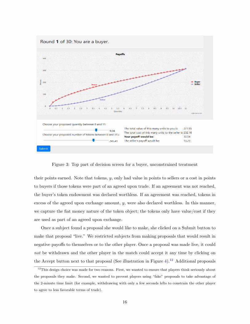
Figure 3: Top part of decision screen for a buyer, unconstrained treatment

their points earned. Note that tokens, y, only had value in points to sellers or a cost in points

to buyers if those tokens were part of an agreed upon trade. If an agreement was not reached,

the buyer’s token endowment was declared worthless. If an agreement was reached, tokens in

excess of the agreed upon exchange amount, y, were also declared worthless. In this manner,

we capture the fiat money nature of the token object; the tokens only have value/cost if they

are used as part of an agreed upon exchange.

Once a subject found a proposal she would like to make, she clicked on a Submit button to

make that proposal “live.” We restricted subjects from making proposals that would result in

negative payoffs to themselves or to the other player. Once a proposal was made live, it could

not be withdrawn and the other player in the match could accept it any time by clicking on

the Accept button next to that proposal (See illustration in Figure 4).12 Additional proposals

12This design choice was made for two reasons. First, we wanted to ensure that players think seriously about

the proposals they make. Second, we wanted to prevent players using “fake” proposals to take advantage of

the 2-minute time limit (for example, withdrawing with only a few seconds lefts to constrain the other player

to agree to less favorable terms of trade).

16

Figure 4: Bottom part of decision screen for a buyer, unconstrained treatment

made by either player within the 2 minute round were added to the existing set of proposals

and did not replace any prior proposal.

Buyers and sellers could see each others’ submitted proposals at all times under columns

for buyer and seller proposals. If there were many proposals made in a round, then a scroll-bar

appeared allowing subjects to review all live proposals. Proposals were only live for duration

of each 2 minute round; the set of proposals was cleared out at the start of each new round.

A round ended when either a proposal was agreed to or the 2 minute time limit had expired,

whichever came first. Importantly, our experiment was implemented in two phases. In the

first phase, we explored the unconstrained treatment (where m = 315) in order to estimate

the bargaining weight, θ. As noted earlier, we picked m = 315, as it was well above u(q∗). In

the unconstrained treatment, we found strong evidence that θ = 1/2, as shown in Section 5.2.

With that knowledge, we designed the second phase of the experiment, where we studied

environments where the buyer’s money holdings were sufficiently low that the first best could

17

not be achieved. Specifically, in the constrained treatments, m = 60 and m = 30.13

As Figure 2 shows in these constrained cases, the buyer’s surplus under the Nash solution

is first increasing and then decreasing, whereas under the Kalai solution, the buyer’s surplus

is strictly increasing and is equal to the seller’s surplus in all three treatments. Note that in

the unconstrained case, the Nash and Kalai solutions coincide.

Summarizing, our three treatments involve three different values for m:

1. Unconstrained: m = 315 ≥ u(q∗)

2. Constrained-High: m = 60 < c(q∗)

3. Constrained-Low: m = 30 < c(q∗).

4.3 Hypotheses

Table 1 provides predictions for q, y, the per unit price y/q, the seller and buyer’s surpluses,

Ss and Sb, the total surplus, S, and the ratio of the buyer’s surplus to the total surplus, Sb

S ,

under the Nash and Kalai bargaining solutions in the θ = 1/2 case for all three treatments.14

Based on the theoretical predictions, we have the following hypotheses.

Hypothesis 1. In the unconstrained case, subjects achieve the first best.

This hypothesis checks whether there are any inefficiencies in the unconstrained case.

Hypothesis 2. As m increases, the agreed upon q, the amount of tokens spent y, the

total surplus S, and the seller’s surplus Ss all increase.

Hypotheses 1 and 2 are valid under both bargaining solutions and are independent of θ.

However, the buyer’s surplus, Sb, may increase or decrease in m depending on the bargaining

solution.

Hypothesis 3a (Nash) As m increases, the buyer’s surplus, Sb, is increasing and then

decreasing as q increases toward q∗.

Hypothesis 3b (Kalai) As m increases, the buyer’s surplus, Sb, is monotonically in-

creasing as q increases toward q∗.

13While we conducted our experiment in two stages, we employed a between subjects design. Each subject

participated in only a single treatment, either m = 315, m = 60 or m = 30.14We use predictions for the θ = 1/2 case because, as we show below in Section 5.2, this is the empirical

estimate for θ that emerges in the unconstrained case.

18

Table 1: Theoretical predictions, Nash vs. Kalai, θ = 1/2.

m = 315 q y y/q Ss Sb S SbS

Nash 4 118.91 29.73 51.5 51.5 103 .5

Kalai 4 118.91 29.73 51.5 51.5 103 .5

m = 60 q y y/q Ss Sb S SbS

Nash 2.17 60 27.65 33.27 58.19 91.46 .64

Kalai 1.69 60 35.5 41.71 41.71 83.42 .5

m = 30 q y y/q Ss Sb S SbS

Nash 1.24 30 24.19 19.59 54.4 73.99 .74

Kalai 0.625 30 48 25.96 25.96 51.92 .5

Hypothesis 3a is the prediction of the Nash bargaining solution, while hypothesis 3b is the

prediction of the Kalai bargaining solution.

5 Results

In this section we first report on the number of sessions and results relevant to the question

of the appropriate bargaining weight and solution. Then, we report on an analysis of the

bargaining process data.

5.1 Sessions, Subjects and Payments

The experiment was programmed in oTree (Chen et al. (2016)) and was conducted over net-

worked computers in the Experimental Social Science Laboratory at UC Irvine. Subjects were

undergraduate students from a variety of different majors and had no prior experience with

our study. The were recruited using Sona Systems software. At the start of each 90 minute

session, subjects were given written instructions which were read out loud. All participants

had to successfully complete comprehension test questions before proceeding to the bargaining

task. Sample instructions and comprehension test questions are found in Appendix A.

19

Following the instructions and test which took about 30 minutes, the remaining hour was

devoted to the 30 bargaining rounds (maximum of 2 minutes each).

As noted earlier, subjects earned points in each round depending on bargaining outcomes.

At the end of the session two rounds were randomly chosen. The sum of subjects’ point totals

from those two rounds were multiplied by 0.25 to determine subjects’ monetary earnings

from the bargaining task. In addition, subjects earned a $7 show up payment. Table 2

provides details concerning the number of sessions and the average payoffs including the show-

up payment.

Table 2: Sessions and Average Earnings.

Treatment Session No. Average Earnings

m=315 1 $30.25

m=315 2 $32.75

m=315 3 $29.66

m=315 4 $32.68

m=315 5 $30.09

m=60 1 $26.39

m=60 2 $27.81

m=60 3 $25.18

m=60 4 $27.84

m=60 5 $25.83

m=30 1 $19.51

m=30 2 $18.07

m=30 3 $19.34

m=30 4 $18.55

m=30 5 $19.70

20

Table 3: Random-effect estimation of the buyer’s share of surplus in accepted offers.

Buyer’s surplus

(1) (2) (3) (4)

Total surplus, S 0.5012 0.4994 0.4987 0.4989

(0.0032) (0.0018) (0.0019) (0.0019)

Observations 698 574 412 348

Standard errors clustered at the session level in parentheses

5.2 Estimation of the Bargaining Weight

Our first result concerns the buyer’s share of the total surplus. We examine the buyer’s share

in the unconstrained case because under the Nash and Kalai solutions, the buyer’s share gives

us an estimate of the bargaining weight θ.

To estimate the bargaining weight, we focus on accepted offers and regress the buyer’s

surplus Sbi on the total surplus achieved by each pair, Si. Specifically we run the regression

Sbi = θSi + εi,

using a random effects regression estimator where i indexes an individual buyer.15 We consider

several specifications that vary in terms of how close the quantity is to the first best prediction

of q∗ = 4. Specifically, the sample we use consists of accepted offers in the unconstrained

treatment for four different neighborhoods of q∗ = 4:

(1) all (2) s.t. |q − 4| < 0.5

(3) s.t. |q − 4| < 0.1 (4) s.t. |q − 4| < 0.05.

The results are reported in Table 3. We see that regardless of any restrictions placed on traded

quantities q, the estimate θ is not statistically different from 0.5.

Finding 1. The buyer’s share of the surplus in the unconstrained case is equal to 0.5.

15Regression results obtained when random effects are indexed at the individual seller level are reported in

Table D3 in Appendix D.

21

Table 4: Average agreed-upon outcomes by treatment.

q y yq Ss Sb S Sb

S

m = 315 4.03 119.67 29.82 50.99 51.09 102.08 .50

m = 60 1.69 59.05 35.88 40.65 42.14 82.79 .50

m = 30 0.67 29.70 47.19 25.09 28.11 53.21 .52

Finding 1 suggests that we can use θ = 1/2 to evaluate our theoretical predictions in the

constrained case, where they differ among the two solutions. The predictions for the case

where θ = 1/2 were reported earlier in Table 1.

5.3 Which solution?

Figure 5 shows the distribution of traded quantities and tokens over all five sessions of each

of the three treatments. Mean values are reported in Table 4.16 Figure 5 and Table 4, in

conjunction with Table 1, which reports the theoretical predictions for θ = 1/2, indicate that

there is overall support for aspects of the theoretical predictions captured in Hypotheses 1

and 2, and more support for the Kalai solution, as formalized in Hypotheses 3b. We provide

a more rigorous analysis of the data next.

We focus first on the unconstrained case, where we see that in case of agreement, the mean

traded quantity is 4.03 and the mean traded tokens are 119.69. Using a Wilcoxon signed-rank

test on session-level averages for agreed upon trades, we find that we cannot reject the null

hypothesis that in the unconstrained treatment, q = 4 and y = 118.91, i.e., the first best is

achieved (p-values=.626 and .4375, respectively).

Finding 2. Consistent with Hypothesis 1, in the unconstrained case, we cannot reject the null

that subjects achieve the first best.

We next consider traded quantities and tokens across all three treatments. In addition to

the averages displayed in Table 4, histograms show the distributions of traded quantities and

tokens in Figure 5.

16Means by session and for each first/last 15 rounds are provided in Appendix D in Table D2.

22

Figure 5: Distribution of traded quantities and tokens by treatment.

Finding 3. Consistent with Hypothesis 2, as m increases, the traded quantity q, the amount

of tokens spent y, the total surplus S and the seller’s surplus Ss all increase.

Support for Finding 3 is found in rows 1-4 of Table 5, which reports results from non-

parametric Jonckheere tests for ordered alternatives using session-level average data over all

periods, and the first and second halves of each session (periods 1-15 and 16-30). Specifically,

we test the null hypothesis that population medians for each treatment value for m (xm) for

the variables q, y, and S, Ss are the same, i.e., H0: x30 = x60 = x315, against the ordered

alternative hypothesis predicted by theory: HA: x30 ≤ x60 ≤ x315, with at least one strict

inequality. We find that we can easily reject the null in favor of the alternative in all cases.

Next, we study the impact of varying the liquidity constraint, m, on the buyer’s surplus,

so as to discriminate between Hypotheses 3a and 3b.

Finding 4. Consistent with Hypothesis 3b (Kalai) but counter to Hypothesis 3a (Nash) the

buyer’s surplus is monotonically increasing as m increases.

23

m = 30 m = 60 m > 171

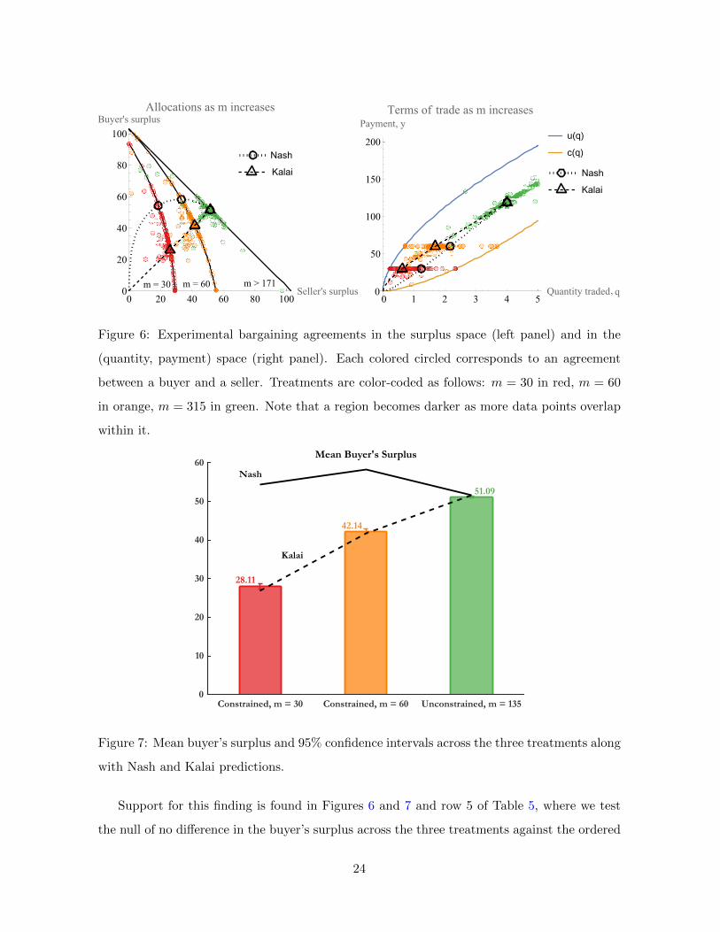
Figure 6: Experimental bargaining agreements in the surplus space (left panel) and in the

(quantity, payment) space (right panel). Each colored circled corresponds to an agreement

between a buyer and a seller. Treatments are color-coded as follows: m = 30 in red, m = 60

in orange, m = 315 in green. Note that a region becomes darker as more data points overlap

within it.

Mean Buyer's Surplus

28.11

42.14

51.09

Kalai

Nash

Constrained, m = 30 Constrained, m = 60 Unconstrained, m = 1350

10

20

30

40

50

60

Figure 7: Mean buyer’s surplus and 95% confidence intervals across the three treatments along

with Nash and Kalai predictions.

Support for this finding is found in Figures 6 and 7 and row 5 of Table 5, where we test

the null of no difference in the buyer’s surplus across the three treatments against the ordered

24

Table 5: Results and p-values from Jonckheere tests of ordered alternatives for the variables,

q, y, S, Ss and Sb, all periods, first half (periods 1-15) and second half (periods 16-30), using

session-level average data.

Row No., Hypotheses: All First Half Second Half

Variable H0 vs. HA periods Periods 1-15 Periods 16-30

1 H0 : q30 = q60 = q315 Reject H0 Reject H0 Reject H0

q HA : q30 ≤ q60 ≤ q315 p = .0000 p = .0000 p = .0000

2 H0 : y30 = y60 = y315 Reject H0 Reject H0 Reject H0

y HA : y30 ≤ y60 ≤ y315 p = .0000 p = .0000 p = .0000

3 H0 : S30 = S60 = S315 Reject H0 Reject H0 Reject H0

S HA : S30 ≤ S60 ≤ S315 p = .0000 p = .0000 p = .0000

4 H0 : Ss30 = Ss60 = Ss315 Reject H0 Reject H0 Reject H0

Ss HA : Ss30 ≤ Ss60 ≤ Ss315 p = .0000 p = .0000 p = .0000

5 H0 : Sb30 = Sb60 = Sb315 Reject H0 Reject H0 Reject H0

Sb HA : Sb30 ≤ Sb60 ≤ Sb315 p = .0000 p = .0000 p = .0000

alternative predicted by the Kalai (but not by the Nash) solution, using session-level average

data. We find that we can reject the null of no difference in favor of the alternative that the

buyer’s surplus Sb, increases as m increases from 30 to 60 to 315, which is consistent with the

Kalai solution.17

To quantify these effects, we also run the regression

Sbi = β11{m=30} + β21{m=315} + εi, (7)

using a random effects regression estimator where i indexes an individual buyer. We focus on

accepted offers, and report results for two different specifications:

17We also tested the null hypothesis that the buyer’s surplus was equal in pairwise comparisons between the

three treatments using non-parametric Mann Whitney tests on session-level average data, i.e., Sb30 vs. Sb60; Sb60

vs. Sb315; Sb30 vs. Sb315; We are always able to reject the null of no difference in favor of the alternative that the

buyer’s surplus is higher when m is higher (p = .0079 for all three two-sided tests), which again favors the Kalai

solution and runs counter to the non-monotonic prediction for the buyer’s surplus under the Nash solution.

25

Table 6: Random-effects estimation of the impact of varying the liquidity constraint, m, on

the buyer’s surplus.

Buyer’s surplus

(1) (2)

m = 30 -13.9488 -14.2499

(1.0885) (1.1902)

m = 315 8.9191 9.0271

(0.8067) (0.8106)

Constant (m = 60) 42.1993 42.3712

(0.7856) (0.7943)

Observations 2028 1801

Standard errors clustered at the session level in parentheses

(1) all accepted offers

(2) accepted offers s.t. |q − 4| < 0.5 when m = 315, y − 60 < 0.5 when m = 60, and

y − 30 < 0.5 when m = 30.18

The results are reported in Table 6.19 For both specifications, consistent with Kalai’s pre-

dictions, the buyer’s surplus significantly decreases when m is reduced from 60 to 30, and

significantly rises when m is increased from 60 to 315.

5.4 Discussion

Given the estimated bargaining weight of θ = 0.5, the Kalai solution coincides with the

“efficient equal split” outcome, or the case where the buyer and seller surpluses are maximized

subject to the constraint that both surpluses are equal. Efficient equal split is not a general

18These conditions ensure that offers are close to the Pareto frontier, i.e., players are close to behaving

rationally by proposing a Pareto-efficient joint production.19Regression results obtained when random effects are indexed at the individual seller level are reported in

Table D4 in Appendix D.

26

property of the Kalai solution. For values of θ different from 0.5, one can show that 1) buyer

and seller’s surpluses will not be equal under the Kalai solution; 2) in the presence of liquidity

constraints, total earnings efficiency remains lower under the Kalai solution as compared with

the Nash solution.

We do not pursue here the exercise of varying θ, as that would involve adding more

structure to our bargaining game and complicate interpretations across treatments; in the

present setup, θ does not enter explicitly as a parameter affecting choices anywhere in our

game as it is a model primitive. Instead, θ is estimated using data for the case where buyers

are not liquidity constrained. Further, we have no reason to think that θ would change as

liquidity constraints become binding, as existing theory is silent on this issue.

As a thought exercise, however, suppose we fixed the buyer’s share, Sb/S = 0.5, and asked

how the bargaining weight would have to change as the liquidity constraint became binding

so as to make the allocation consistent with the Nash solution rather than the Kalai solution.

This is equivalent to solving for θN such that Θ(q) = 0.5. We obtain

θN =c′(q)

u′(q) + c′(q). (8)

Plugging in the values for q predicted by the Kalai solution for m ∈ {30, 60, 315} into (8), we

respectively obtain θN = 0.15, θN = 0.31, and θN = 0.5. That is, large changes in θN across

environments would be needed in order for the Nash solution to fit the data.

6 The Bargaining Process

In this section we consider the process by which buyers and sellers reached a trade agreement

in each two minute round.

Overall, 91% of negotiations ended with an agreement. More specifically, the looser the

constraint on tokens, the higher the agreement rate: 89% for m = 30, 91% for m = 60 and

94% for m = 315. Table D1 in Appendix D reports agreement rates for the first 15 and the

last 15 rounds, by session.

Figure 8 shows the share of the surplus that buyers assign to themselves as part of their

offers, as the negotiation unfolds. The three panels correspond to the three treatments. The

sample is restricted to negotiations that ended with an agreement during sessions 1 to 6.20 In

20The sample here is restricted to the first six sessions because timestamps tracking the order in which

27

each panel, offers are ranked by their order relative to the last offer made. For example, in

the left panel, the yellow dots represent all the fourth-to-last offers made by buyers (i.e., the

third subsequent offer was the agreed-upon offer). The black square represents the median

offer in this sample, and the black cross the average. We can see that buyers start out making

proposals that significantly favor themselves (above the 0.5 equal split line), but they adjust

these proposals downward as the negotiation proceeds. The bargaining process is similar for

sellers, who also start out making proposals that greatly favor themselves before agreeing to

approximately equal splits as the bargaining time limit approaches (see Figure E1 in Appendix

E).

This process data analysis reveals that subjects do not immediately jump to the final

outcome where the total surplus is split equally as reported in Section 5. That is, the equal

split final outcome is not due to an inherent desire for fairness on the part of players. Rather,

subjects initially try to extract more surplus for themselves and only converge to an equal

split as a result of the back-and-forth bargaining process.

To obtain an estimate of the compromises made by players as the negotiation unfolds, we

study a new variable,

∆ player’s share = player’s share in first offer round − agreed-upon player’s share.

We then regress this new variable on a dummy variable indicating whether the player or her

negotiation partner made the first offer. Observations include all rounds that ended with

an agreement in sessions 1 to 6. Since each recorded offer corresponds to two observations

(one recorded for the buyer and one recorded for the seller), we run two separate regressions,

splitting the sample by roles. Results for the sample restricted to buyers are presented in

Table 7 while results for the sample restricted to sellers are available in Appendix D in Table

D5.

When the player makes the first offer, she initially proposes to allocate to herself a share of

the total surplus that is, on average, 8.71 percentage points higher than is eventually agreed-

upon. On the other hand, if her trade partner made the first offer, the player eventually

obtains a share of the total surplus that is, on average, 4.80 percentage points higher than

was originally proposed. Finding 5 summarizes this analysis. Similar conclusions can be made

proposals were made were not recorded for subsequent sessions.

28

4th to last 3rd to last 2nd to last Last

Buyer's Offer

0.35

0.4

0.45

0.5

0.55

0.6

0.65

Bu

yer'

s sh

are

of

surp

lus

m = 30

4th to last 3rd to last 2nd to last Last

Buyer's Offer

0.35

0.4

0.45

0.5

0.55

0.6

0.65

Bu

yer'

s sh

are

of

surp

lus

m = 60

4th to last 3rd to last 2nd to last Last

Buyer's Offer

0.35

0.4

0.45

0.5

0.55

0.6

0.65

Bu

yer'

s sh

are

of

surp

lus

m = 315

Median

Mean

Figure 8: Buyers’ share of the surplus in their own offers, by rank of the offer relative to

the accepted offer and by treatment. Colored circles represent all offers. Median offers are

represented with a black square, and mean offers are represented by a black cross.

Table 7: Random-effect estimation of the change in a player’s share of surplus between the

first offer and the accepted offer, dependent on having made the first offer. Random effects

are indexed at the individual player level. Sample is restricted to buyers.

∆ Player’s share

Player made the first offer -0.1351

(0.0222)

Constant 0.0480

(0.0089)

Observations 835

Standard errors clustered at the session level in parentheses

29

Table 8: Average number of proposals made by a pair of players during one round.

Type of negotiation

All Agreement No agreement

All treatments

All rounds 7.22 6.84 11.15

1-15 6.65 6.21 10.47

16-30 7.79 7.44 12.11

m = 30

All rounds 11.37 10.98 14.31

1-15 9.98 9.49 13.29

16-30 12.75 12.43 15.63

m = 60

All rounds 5.44 5.23 7.55

1-15 5.05 4.8 7.24

16-30 5.84 5.66 7.93

m = 315

All 4.85 4.48 10.43

1-15 4.93 4.47 9.91

16-30 4.77 4.49 11.53

when the sample is restricted to sellers.

Finding 5. If more than one proposal is made, the initial proposal is more favorable to the

player making the proposal than is the final agreed upon proposal.

Note that the bargaining process delineated above, with both players starting by propos-

ing higher shares of surplus to themselves before converging towards a potential agreement,

generates delays. Table 8 shows the average number of proposals made by a pair of play-

ers during one round (over the entire sample), broken down across treatments, rounds, and

whether bargaining ended with an agreement. On average, players made 7.22 proposals per

round. This number is markedly higher for rounds that did not end up with an agreement.

While we do not have timed evidence, this finding suggests that players who agreed on a trade

were typically not constrained by the time limit, since they typically made fewer offers than

their counterparts who did not agree. It is also interesting to note that the more stringent is

the liquidity constraint, the greater is the number of offers made on average by the players

30

(and thus the larger the delays): it took fewer than 5 proposals, on average, for players in the

unconstrained treatment to agree, compared to almost 11 proposals for players in the most

constrained treatment.

7 Welfare Cost of Inflation

The results we reported on in the previous section provide strong support for the Kalai bar-

gaining solution over the Nash solution and for equal bargaining weights for buyers and sellers.

In this section we show how these findings can be of use to researchers working in the search-

money literature, who make use of the bargaining setting that our experiment studies. In

particular, we show how our findings on bargaining weights and bargaining solution have

important implications for the estimation of the welfare costs of inflation.21

Consider the inverse demand curve for real money balances, with money demand on the

x-axis and the nominal interest rate on the y-axis. The empirical money demand curve is

represented by the circles in Figure 9 for the years 1900-2000, where each observation cor-

responds to a year. Money demand corresponds to the aggregate balance of M1 divided by

nominal GDP, while the nominal interest rate corresponds to the rate on short-term commer-

cial paper. The original method developed to estimate the welfare cost of inflation is due to

Bailey (1956) and was later expanded upon by Lucas (2000). It consists in first estimating

the demand curve and then measuring the area under the curve between the relevant nominal

interest rates, where the latter are mapped into inflation rates (Π) using the Fisher equation,

i = r + Π.

Craig and Rocheteau (2006, 2008) highlight that the Bailey-Lucas approach is only correct

if the private benefits of real money balances to money holders are equal to their social benefits.

Indeed, the money demand curve only captures the benefits of money to its holders, not to

society. Since any transaction is two-sided, conditional on sellers extracting some surplus from

transactions, the welfare triangle approach underestimates the benefits of real money balances

(and thus underestimates the cost of inflation). Obtaining a correct estimate therefore requires

21We recognize that this section may not appeal to all readers, but the question of the appropriate bargaining

solution to use in search-money models and the implications for the welfare cost of inflation did serve as an

impetus for this project, and so we feel we would be remiss not to include this discussion here. Readers who

are not interested in this topic can skip to the concluding section 8.

31

0.05 0.1 0.15 0.2 0.25 0.3 0.35 0.4 0.45 0.5

Money demand

0.01

0.03

0.05

0.07

0.09

0.11

0.13

0.15

No

min

al

inte

rest

rate

Data

Fitted Curve

Figure 9: Money demand curve in the US, 1900-2000. Empirical observations in black circles

(source: Craig and Rocheteau, 2006). Non-linear least square curve fit for θ = 0.5 under the

Kalai bargaining solution in orange solid curve.

accounting for the surplus obtained by sellers in transactions. For a given surplus received

by a buyer (money holder), the surplus received by the seller depends entirely on the way in

which terms of trade are determined. For example, in a transaction where the buyer receives

a surplus Sb, the seller would receive a surplus Ss = (1− θ) Sb/θ, assuming Kalai bargaining

with a buyer’s bargaining weight of θ. A different bargaining solution or a different distribution

of bargaining powers would lead to inferring a different surplus for the seller.

Using a typical search-theoretical model of money where competitive markets alternate

with decentralized markets with bilateral trades that make money essential, Craig and Ro-

cheteau (2006, 2008) are then able to estimate the welfare cost of inflation for four different

trading protocols (fixed markup, Nash bargaining, Kalai bargaining, and take-it-or-leave-it

offers) and a variety of distributions of bargaining powers. They calibrate their model to the

US economy between 1900 and 2000.

We follow a similar method but calibrate the decentralized market to reflect our experi-

32

mental setup. Specifically, we estimate the money demand curve and the cost of inflation using

the parameters from the experiment, varying both the distribution of bargaining powers and

the bargaining protocol assumed.22 Following the literature, we focus on estimating the cost

of a 10% inflation regime compared to a no-inflation regime. Given a discount rate of 3%, this

is equivalent to comparing an economy with a i = 13% nominal interest rate to an economy

with a i = 3% nominal rate. Note that a nominal interest rate of 0% (thus an inflation rate

of -3%) corresponds to the Friedman rule.

Table 9 shows our results. Considering both the Kalai and Nash bargaining solutions, the

Table 9: Estimates of the quantities traded bilaterally and of the welfare cost of inflation.Buyer’s bargaining Quantity traded, q Welfare cost (% of GDP),

power, θ i = 0% (Friedman rule) i = 3% (No inflation) i = 13% (10% inflation) from i = 3% to i = 13%

Kalai

0.33 4.00 2.84 0.32 5.70

0.50 4.00 2.70 0.43 3.35

0.66 4.00 2.70 0.74 2.13

1.00 4.00 3.06 1.68 1.20

Nash

0.33 1.54 1.04 0.51 3.67

0.50 2.17 1.53 0.76 2.86

0.66 2.74 1.98 1.02 2.26

1.00 4.00 3.06 1.68 1.20

table reports the quantity traded in bilateral meetings as well as the cost of 10% inflation as

a function of the buyer’s bargaining weight.

First notice that the higher is the inflation rate, the higher is the nominal interest rate,

and the lower is the quantity that is traded, q. Indeed, the higher the inflation rate, the

more costly it is to hold real money balances from one period to the next (in other words, the

nominal interest rate is the opportunity cost of holding real money balances). As this cost

increases, buyers economize by carrying fewer real balances, and thus they cannot purchase

as many units of the consumption good from sellers. This phenomenon is partially due to

a hold up problem: as long as θ < 1, buyers do not extract all of the surplus generated by

carrying real balances, which leads them to “underinvest” in real balances. This disappears

when θ = 1, in which case the first-best quantity of goods is traded both under the Nash and

Kalai bargaining solutions, q = q∗ = 4. Interestingly, note that under the Nash solution, even

when the Friedman rule is in place so that carrying real money balances is costless (i = 0),

buyers may not carry the optimal amount of real balances, leading to suboptimal trade sizes.

22See Appendix C for details about the model and the estimation.

33

This is due to the non-monotonicity of the Nash solution, as depicted in Figure 2. At some

point, carrying additional real balances worsens the buyer’s bargaining position under the

Nash solution as it reduces the amount of the surplus that she can extract. Even if real money

balances are costless, this is another reason for buyers to limit their money holdings.23

Estimates obtained under the specification in line with our experimental results are high-

lighted in grey. The corresponding estimated money demand curve is represented in Figure 9.

Finding 6. Under Kalai bargaining and with a buyer’s bargaining power of 0.5, the cost of a

10% inflation amounts to 3.35% of GDP. Assuming instead that buyers have all the bargaining

power (θ = 1) leads to underestimating the welfare cost of inflation by a factor of 2.79 (for

a cost of 1.20% of GDP). Setting the bargaining power equal to θ = 0.5 but using the Nash

bargaining solution instead of Kalai leads to underestimating the cost of inflation by a factor

of 1.17 (for a cost of 2.86% of GDP).

8 Conclusion

We have studied a bargaining setting where players simultaneously determine both the size

of the gains from trade and the division of those gains. We have further considered the case

where one party, the buyer, is constrained in terms of the amount of money that they can

bring to the bargaining table. Such liquidity constraints are a common phenomenon and

make the bargaining set asymmetric between the two players. Under the Nash bargaining

solution, the presence of liquidity constraints gives rise to a larger surplus going to the buyer

relative to the seller and larger total gains from trade than under the Kalai solution, where

the surpluses are predicted to be equal (given the bargaining weight of 1/2) regardless of

liquidity constraints. These two different solutions are used in the money search literature to

understand such questions as the welfare cost of inflation.

The evidence from our experiment clearly favors the Kalai bargaining solution over the

Nash solution. Still, this is just a first step in understanding how liquidity constrained players

approach the bargaining problem.

23An interesting result is that while in partial equilibrium, for a given amount of money holdings, the Nash

bargaining leads to a higher total surplus shared between a buyer and a seller, in general equilibrium, Nash

bargaining leads to lower real money balances holdings and therefore lower surpluses.

34

It is interesting to note that by favoring a solution close to the proportional Kalai bar-

gaining solution rather than Nash bargaining, players effectively agree to share a smaller pie,

decreasing total welfare, in order to achieve more equality. The Nash solution would allow for

a larger joint production, albeit at the expense of the seller. Theory predicts that this welfare

result would be overturned were the liquidity constraints endogenized through a costly ex-ante

choice of real balances by buyers (see, e.g., Lebeau (2020), Rocheteau et al. (2020)). In that

case, playing according to the Nash solution rather than the Kalai solution would lead the

buyer to carry fewer real balances, making the negotiation more liquidity-constrained, even-

tually resulting in lower trade volumes and total welfare. In that case, it would also be to the

advantage of the buyer to implement Kalai bargaining. This suggests that our findings would

be strengthened were liquidity constraints endogenized rather than imposed upon subjects.

A promising avenue to test this hypothesis in the lab would be to consider the following

two stage game. First buyers decide how much to borrow in terms of money. Then, in the

second stage, bargaining takes place. Finally, in the payoff stage, buyers have to repay their

borrowings with interest and realize their payoffs. Higher interest rates would also capture

higher inflation rates, allowing us to explore the welfare costs of inflation more directly.

Other promising investigations include the implementation of bargaining settings that

provide non-cooperative foundations to Kalai’s solution (see, e.g., Dutta (2012, 2021), Hu and

Rocheteau (2020)) as well as the incorporation of unstructured bargaining in fully dynamic

settings (e.g., Duffy and Puzzello (2021), Jiang et al. (2021)). We leave these extensions to

future research.

References

Anbarci, N. and N. Feltovich (2013): “How sensitive are bargaining outcomes to changes

in disagreement payoffs?” Experimental Economics, 16, 560–596, https://doi.org/10.

1007/s10683-013-9352-1.

——— (2018): “How fully do people exploit their bargaining position? The effects of bargain-

ing institution and the 50–50 norm,” Journal of Economic Behavior & Organization, 145,

320–334, https://doi.org/10.1016/j.jebo.2017.11.020.

35

Aruoba, S. B., G. Rocheteau, and C. Waller (2007): “Bargaining and the Value of

Money,” Journal of Monetary Economics, 54, 2636–2655, http://dx.doi.org/10.1016/

j.jmoneco.2007.07.003.

Aruoba, S. B., C. J. Waller, and R. Wright (2011): “Money and capital,” Journal of

Monetary Economics, 58, 98–116, https://doi.org/10.1016/j.jmoneco.2011.03.003.

Bailey, M. J. (1956): “The welfare cost of inflationary finance,” Journal of Political Econ-

omy, 64, 93–110, https://doi.org/10.1086/257766.

Bethune, Z., M. Choi, and R. Wright (2019): “Frictional goods markets: Theory and

applications,” The Review of Economic Studies, 87, 691–720, https://doi.org/10.1093/

restud/rdz049.

Binmore, K., C. Proulx, L. Samuelson, and J. Swierzbinski (1998): “Hard bargains

and lost opportunities,” The Economic Journal, 108, 1279–1298, https://doi.org/10.

1111/1468-0297.00343.

Binmore, K., A. Shared, and J. Sutton (1989): “An outside option experiment,” The

Quarterly Journal of Economics, 104, 753–770, https://doi.org/10.2307/2937866.

Bolton, G. E. and E. Karagozoglu (2016): “On the influence of hard leverage in a

soft leverage bargaining game: The importance of credible claims,” Games and Economic

Behavior, 99, 164–179, https://doi.org/10.1016/j.geb.2016.08.005.

Butler, C. K., M. J. Bellman, and O. A. Kichiyev (2007): “Assessing power in spa-

tial bargaining: When is there advantage to being status-quo advantaged?” International

Studies Quarterly, 51, 607–623, https://doi.org/10.1111/j.1468-2478.2007.00466.x.

Camerer, C. F. (2003): Behavioral game theory: Experiments in strategic interaction,

Princeton university press.

Camerer, C. F., G. Nave, and A. Smith (2019): “Dynamic unstructured bargaining with

private information: theory, experiment, and outcome prediction via machine learning,”

Management Science, 65, 1867–1890, https://doi.org/10.1287/mnsc.2017.2965.

36

Chen, D. L., M. Schonger, and C. Wickens (2016): “oTree—An open-source platform for

laboratory, online, and field experiments,” Journal of Behavioral and Experimental Finance,

9, 88–97, https://doi.org/10.1016/j.jbef.2015.12.001.

Craig, B. and G. Rocheteau (2006): “Inflation and welfare: A search approach,” Federal

Reserve Bank of Cleveland Policy Discussion Paper, 06-12.

——— (2008): “Inflation and welfare: A search approach,” Journal of Money, Credit and

Banking, 40, 89–119, https://doi.org/10.1111/j.1538-4616.2008.00105.x.

Davoodalhosseini, S. M. (2021): “Central bank digital currency and monetary policy,”

Journal of Economic Dynamics and Control, 104150, https://doi.org/10.1016/j.jedc.

2021.104150.

Duffy, J. and D. Puzzello (2021): “The Friedman Rule: Experimental Evidence,” Inter-

national Economic Review, forthcoming, https://doi.org/10.1111/iere.12549.

Dufwenberg, M., M. Servatka, and R. Vadovic (2017): “Honesty and informal agree-

ments,” Games and Economic Behavior, 102, 269–285, https://doi.org/10.1016/j.geb.

2016.12.008.

Dutta, R. (2012): “Bargaining with revoking costs,” Games and Economic Behavior, 74,

144–153, https://doi.org/10.1016/j.geb.2011.06.006.

——— (2021): “Bargaining as a struggle between competing attempts at commitment,” Work-

ing Paper 1, https://dx.doi.org/10.2139/ssrn.3800521.

Feltovich, N. and J. Swierzbinski (2011): “The role of strategic uncertainty in games:

An experimental study of cheap talk and contracts in the nash demand game,” European

Economic Review, 55, 554–574, https://doi.org/10.1016/j.euroecorev.2010.07.001.

Galeotti, F., M. Montero, and A. Poulsen (2019): “Efficiency versus equality in bar-

gaining,” Journal of the European Economic Association, 17, 1941–1970, https://doi.

org/10.1093/jeea/jvy030.

37

Gross, D. B. and N. S. Souleles (2002): “Do liquidity constraints and interest rates

matter for consumer behavior? Evidence from credit card data,” The Quarterly Journal of

Economics, 117, 149–185, https://doi.org/10.1162/003355302753399472.

Guth, W. and M. G. Kocher (2014): “More than thirty years of ultimatum bargaining ex-

periments: Motives, variations, and a survey of the recent literature,” Journal of Economic

Behavior & Organization, 108, 396 – 409, https://doi.org/10.1016/j.jebo.2014.06.

006.

Guth, W., R. Schmittberger, and B. Schwarze (1982): “An experimental analysis of

ultimatum bargaining,” Journal of Economic Behavior & Organization, 3, 367–388, https:

//doi.org/10.1016/0167-2681(82)90011-7.

Heckathorn, D. (1978): “A paradigm for bargaining and a test of two bargaining models,”

Behavioral Science, 23, 73–85, http://dx.doi.org/10.1002/bs.3830230204.

Hoffman, E. and M. L. Spitzer (1982): “The Coase theorem: Some experimental tests,”

The Journal of Law and Economics, 25, 73–98, https://doi.org/10.1086/467008.

——— (1985): “Entitlements, rights, and fairness: An experimental examination of subjects’

concepts of distributive justice,” The Journal of Legal Studies, 14, 259–297, https://doi.

org/10.1086/467773.

Hu, T.-W. and G. Rocheteau (2020): “Bargaining under liquidity constraints: Unified

strategic foundations of the Nash and Kalai solutions,” Journal of Economic Theory, 189,

105098, https://doi.org/10.1016/j.jet.2020.105098.

Iyer, G. and M. Villas-Boas (2003): “A bargaining theory of distribution channels,”

Journal of Marketing Research, 40, 80–100, https://doi.org/10.1509/jmkr.40.1.80.

19134.

Jiang, J., D. Puzzello, and C. Zhang (2021): “Inflation, Output and Welfare in the

Laboratory,” Working paper.

Kalai, E. (1977): “Proportional solutions to bargaining situations: interpersonal utility

comparisons,” Econometrica, 45, 1623–1630, https://doi.org/10.2307/1913954.

38

Kalai, E. and M. Smorodinsky (1975): “Other solutions to Nash’s bargaining problem,”

43, 513–518, https://doi.org/10.2307/1914280.

Karagozoglu, E. (2012): “Bargaining games with joint production,” in The Oxford Hand-

book of Economic Conflict Resolution, Oxford University Press, 359–372, http://doi.org/

10.1093/oxfordhb/9780199730858.013.0024.

——— (2019): “On “going unstructured” in bargaining experiments,” in The Future of Eco-

nomic Design: The Continuing Development of a Field as Envisioned by Its Researchers,

ed. by J.-F. Laslier, H. Moulin, M. R. Sanver, and W. S. Zwicker, Springer, 295–304,

http://dx.doi.org/10.1007/978-3-030-18050-8_40.

Korenock, O. and D. Munro (2021): “Wage bargaining in a matching market: experimen-

tal evidence,” Labour Economics, 73, https://doi.org/10.1016/j.labeco.2021.102078.

Lagos, R. and R. Wright (2005): “A unified framework for monetary theory and policy

analysis,” Journal of Political Economy, 113, 463–484, https://doi.org/10.1086/429804.

Lebeau, L. (2020): “Credit frictions and participation in over-the-counter markets,” Journal

of Economic Theory, 189, 105100, https://doi.org/10.1016/j.jet.2020.105100.

Li, S. and D. Houser (2020): “Stochastic bargaining in the lab,” Working paper.

Lucas, R. E. (2000): “Inflation and Welfare,” Econometrica, 68, 247–274, https://doi.

org/10.1111/1468-0262.00109.

Merlo, A. and C. Wilson (1995): “A stochastic model of sequential bargaining with

complete information,” Econometrica, 63, 371–399, https://doi.org/10.2307/2951630.

Molico, M. (2006): “The distribution of money and prices in search equilibrium,” Inter-

national Economic Review, 47, 701–722, https://doi.org/10.1111/j.1468-2354.2006.

00393.x.

Nash, J. F. (1950): “The bargaining problem,” Econometrica, 18, 155–162, https://doi.

org/10.2307/1907266.

——— (1953): “Two-person cooperative games,” Econometrica, 21, 128–140, https://doi.

org/10.2307/1906951.

39

Navarro, N. and R. F. Veszteg (2020): “On the empirical validity of axioms in unstruc-

tured bargaining,” Games and Economic Behavior, 121, 117–145, http://dx.doi.org/10.

1016/j.geb.2020.01.003.

Nydegger, R. V. and G. Owen (1974): “Two-person bargaining: An experimental test of

the Nash axioms,” International Journal of Game Theory, 3, 239–249, https://doi.org/

10.1007/BF01766877.

Rocheteau, G., T.-W. Hu, L. Lebeau, and Y. In (2020): “Gradual bargaining in decen-

tralized asset markets,” Review of Economic Dynamics, forthcoming, https://doi.org/

10.1016/j.red.2020.10.008.

Rocheteau, G. and R. Wright (2005): “Money in search equilibrium, in competitive

equilibrium, and in competitive search equilibrium,” Econometrica, 73, 175–202, https:

//doi.org/10.1111/j.1468-0262.2005.00568.x.

Roth, A. E. (1995): Bargaining Experiments, Princeton University Press, 253–348, https:

//doi.org/10.1515/9780691213255-006.

Roth, A. E. and M. W. Malouf (1979): “Game-theoretic models and the role of infor-

mation in bargaining.” Psychological Review, 86, 574, https://psycnet.apa.org/doi/10.

1037/0033-295X.86.6.574.

Roth, A. E. and J. K. Murnighan (1982): “The role of information in bargaining: An

experimental study,” Econometrica, 50, 1123–1142, https://doi.org/10.2307/1911866.

Rubinstein, A. (1982): “Perfect equilibrium in a bargaining model,” Econometrica, 50, 97–

109, https://doi.org/10.2307/1912531.

Venkateswaran, V. and R. Wright (2013): “Pledgability and liquidity: A new monetarist

model of financial and macroeconomic Activity,” Working Paper 19009, National Bureau of

Economic Research, https://doi.org/10.3386/w19009.

Weill, P.-O. (2020): “The Search Theory of Over-the-Counter Markets,”

Annual Review of Economics, 12, 747–773, https://doi.org/10.1146/

annurev-economics-091819-124829.

40

Appendix For Online Publication Only

A Experimental Instructions

Note: The following instructions were used in the constrained m = 60 treatment. Other

instructions are similar.

Welcome to this experiment in the economics of decision-making. Please read these in-

structions carefully as the cash payment you earn at the end of today’s session may depend

on how well you understand these instructions. If you have a question at any time, please

feel free to ask the experimenter. There is no talking for the duration of this 2-hour session.

Please turn off your cell phone and any other electronic devices.

Your Role and Matching

There are 10 participants in today’s session. You will participate in 30 rounds of decision-

making using the networked computer workstations of the laboratory. Prior to the first round,

one-half of participants will be randomly assigned the role of Buyer and the other half the

role of Seller. You will remain in the same role in all 30 rounds.

In each and every round, the computer program randomly and anonymously matches

Buyers and Sellers in pairs. All possible pairings of one Buyer with one Seller are equally

likely in each round. Thus, while the player you are paired with will always be of the opposite

type, they are likely to change from round to round. You will not know the identity of any of

the players you are paired with, nor will they know your identity, even after the experiment

is over.

Your Decision in Each Round

In each round, Sellers can produce a good that is valuable to Buyers only. In each round

Buyers have an endowment of 60 tokens that can be used to purchase units of the good that

Sellers produce. A round involves bargaining between the Buyer and Seller over the quantity

of the good the Seller will produce, q, and the number of tokens, τ , the Buyer will give the

Seller in exchange.

A proposal thus consists of a pair, (q, τ). Quantities, q, can range from 0 to 11, inclusive,

1

in increments of up to 2 decimal places. The number of tokens, τ , can range from 0 to 60,

inclusive, in increments of up to 2 decimal places. Proposals can be made by either the Buyer

or the Seller at any time during each 2-minute bargaining round. Any number of proposals

can be made by either player and in any order over the duration of the bargaining round.

Once a proposal is made, it is shown on both the Buyer and the Seller’s decision screens and

is considered “live”. If the player not making the proposal chooses to accept that proposal,

the bargaining round is declared over and the proposed exchange of q units of the good for τ

tokens is implemented. The payoffs from such an agreed upon exchange are explained below.

Proposals submitted by one player can be accepted by the other player at any time during each

2-minute round. If no proposal is made or there is no agreement on any proposal by players

within each 2-minute bargaining round, then the round is declared over and no exchange takes

place.

Payoffs From Exchange Outcomes

1. If a proposal is accepted within the 2-minute bargaining round, then an exchange takes

place. In that case:

• The Buyer’s payoff is given by:

Buyer’s payoff in points = u(q)− τ. (A1)

Here u(q) is an increasing function of the quantity q representing the buyer’s value

from consuming q units of the good. This function is illustrated on your deci-

sion screen, and Table A1 provides the actual function for u(q) along with a non-

exhaustive list of possible values for u(q). Note that while u(q) is increasing in q,

these increases are lower with higher values for q. Notice also that each token a

Buyer gives to the Seller reduces the Buyer’s payoff by one point. Importantly,

tokens that are not offered as part of an agreed upon proposal have no payoff in

points to the Buyer. That is, if an agreed upon proposal involves an exchange of

τ tokens, then the Buyer loses τ points. Any remaining tokens held by the buyer,

60− τ , have 0 value.

2

Table A1: Buyer values u(q) = (74.1752)q0.6 and Seller costs c(q) = (8.23249)q1.51678 in points.

q u(q) in points c(q) in points Difference u(q)− c(q) pts.

0 0.00 0.00 0.00

0.25 32.29 1.01 31.28

0.5 48.94 2.88 46.06

0.75 62.42 5.32 57.09

1 74.18 8.23 65.94

1.25 84.80 11.55 73.25

1.5 94.60 15.23 79.38

1.75 103.77 19.24 84.53

2 112.43 23.56 88.87

2.25 120.66 28.17 92.50

2.5 128.54 33.05 95.49

2.75 136.10 38.19 97.91

3 143.39 43.57 99.82

3.25 150.45 49.20 101.25

3.5 157.29 55.05 102.24

3.75 163.94 61.12 102.81

4 170.41 67.41 103.00

4.25 176.72 73.90 102.82

4.5 182.89 80.60 102.29

4.75 188.92 87.48 101.44

5 194.82 94.56 100.26

5.25 200.61 101.83 98.79

5.5 206.29 109.27 97.02

5.75 211.87 116.89 94.97

6 217.34 124.69 92.66

6.25 222.73 132.65 90.08

6.5 228.04 140.78 87.26

6.75 233.26 149.07 84.19

7 238.41 157.53 80.88

7.25 243.48 166.14 77.34

7.5 248.48 174.91 73.58

7.75 253.42 183.83 69.59

8 258.29 192.89 65.40

8.25 263.11 202.11 61.00

8.5 267.86 211.47 56.39

8.75 272.56 220.98 51.58

9 277.21 230.63 46.58

9.25 281.80 240.41 41.39

9.5 286.35 250.34 36.01

9.75 290.84 260.40 30.45

10 295.30 270.59 24.71

10.25 299.70 280.92 18.79

10.5 304.07 291.37 12.70

10.75 308.39 301.96 6.43

11 312.68 312.68 0.00

3

• The Seller’s payoff is given by:

Seller’s payoff in points = τ − c(q) (A2)

Each token a Seller receives from a Buyer increases the Seller’s payoff by one point.

Recall that tokens only have value to the Seller in terms of points (and a cost to

the Buyer in terms of points) if a proposal is accepted. Notice also that the Seller’s

payoff is decreased by c(q), which represents the Seller’s cost of producing q units.

This cost function, c(q), is illustrated on your decision screen. Table A1 provides

the actual function for c(q) along with a non-exhaustive list of possible values for

c(q). Note that while c(q) is increasing in q these increases are higher with higher

values for q.

2. If no proposal is made or is accepted within a 2-minute bargaining round then no ex-

change takes place. In that case:

• Both the Buyer and the Seller payoffs are 0 for that round.

The Decision Screen

The decision screen you face is illustrated in Figures 1-2. The top part of this screen, as

shown in Figure 1, illustrates the functions u(q) for Buyers and c(q) for Sellers. Below this

illustration are two slider bars, one for the quantity, q, and the other for tokens, τ , which are

repeated in Figure 2, which illustrates the bottom part of the decision screen from the Buyer’s

perspective (the Seller’s perspective is similar). By moving the slider bars for q and τ you will

see, to the right of these slider bars, how the Buyer’s value, u(q), and the Seller’s cost, c(q),

will be affected by the choice of q as well as the payoff to you and the other player from your

proposal of (q, τ). You can move both slider bars as often as you wish to experiment with

various proposals. When you find a proposal that you would like to submit to the other player,

press the blue Submit button, which makes your proposal ‘live’. This means that the other

player can accept your proposal at any time during the two-minute round. Once submitted,

proposals cannot be withdrawn. Note that proposals that would result in negative payoffs

to either you or the other player are not allowed. The computer program will check whether

4

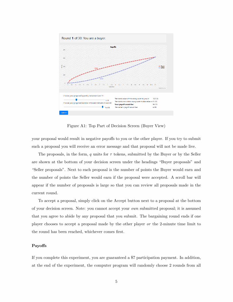
Figure A1: Top Part of Decision Screen (Buyer View)

your proposal would result in negative payoffs to you or the other player. If you try to submit

such a proposal you will receive an error message and that proposal will not be made live.

The proposals, in the form, q units for τ tokens, submitted by the Buyer or by the Seller

are shown at the bottom of your decision screen under the headings “Buyer proposals” and

“Seller proposals”. Next to each proposal is the number of points the Buyer would earn and

the number of points the Seller would earn if the proposal were accepted. A scroll bar will

appear if the number of proposals is large so that you can review all proposals made in the

current round.

To accept a proposal, simply click on the Accept button next to a proposal at the bottom

of your decision screen. Note: you cannot accept your own submitted proposal; it is assumed

that you agree to abide by any proposal that you submit. The bargaining round ends if one

player chooses to accept a proposal made by the other player or the 2-minute time limit to

the round has been reached, whichever comes first.

Payoffs

If you complete this experiment, you are guaranteed a $7 participation payment. In addition,

at the end of the experiment, the computer program will randomly choose 2 rounds from all

5

Figure A2: Bottom Part of Decision Screen (Buyer View)

30 rounds played. Your payoff in points from those 2 rounds will be converted into dollars at

the rate of 1 point = $0.25. Your dollar payoff from the chosen rounds will be added to your

participation payment. Your total payment will be made to you in cash and in private.

Summary of the Experiment

1. Prior to the first round, you will be randomly assigned a role as a Buyer or a Seller. You

will remain in the same role in all 30 rounds of the experiment.

2. In each round, Buyers and Sellers are randomly paired and have 2 minutes to bargain

over an amount, q, of the good the Seller will produce for the Buyer and the amount of

tokens, τ , the Buyer will give the Seller in exchange.

3. Bargaining consists of making proposal pairs of (q, τ). Proposals can be made by either

player, in any order. Proposals that would result in negative payoffs to either player are

not allowed.

4. Once submitted, proposals are considered live and can be accepted at any time.

5. If a proposal, (q, τ), is accepted by the other player, the bargaining round is over. In

that case, the Buyer’s payoff in points for the round is u(q) − τ . The Seller’s payoff in

6

points is τ − c(q).

6. The Buyer’s tokens have no value or cost (i.e., they are worthless) unless a proposal is

accepted. In that case, the τ tokens offered yield τ points to the Seller and cost the

Buyer τ points. Any excess tokens held by the Buyer, 60− τ , have 0 value or cost.

7. If no proposal is made or is accepted within the 2-minute bargaining round, then both

players earn 0 points.

8. At the end of the experiment, 2 rounds, from all 30 rounds, will be randomly chosen for

payment. Your points from those 2 rounds will be converted into dollars at the rate of

1 point = $0.25 cents.

Questions?

Now is the time for questions. If you have a question, please raise your hand and your question

will be answered in private.

Quiz

To check your understanding of the instructions, we ask you to complete the following quiz

before we move on to the experiment. The numbers in these quiz questions are for illustration

purposes only. The actual numbers in the experiment may be quite different. When you have

completed the quiz, please raise your hand. An experimenter will check your answers. If there

are any wrong answers we will go over the relevant part of the instructions again.

1. My role as a Buyer or as a Seller will (circle choice):

a. change every round.

b. remain the same in all rounds.

2. Suppose a player makes a proposal of q = 3.25 and τ = 50, and this proposal is accepted

by the other player. What is the payoff in points to the Buyer from this proposal? (Use

Equation (A1) and Table A1). What is the payoff in points to the Seller from

this proposal? (Use Equation (A2) and Table A1).

7

3. Suppose a player makes a proposal of q = 1 and τ = 60, and this proposal is accepted

by the other player. What is the payoff in points to the Buyer from this proposal? (Use

Equation (A1) and Table A1). What is the payoff in points to the Seller from

this proposal? (Use Equation (A2) and Table A1).

4. If several proposals are made but none are accepted by the end of a 2-minute trading

round, then (circle choice):

a. the last proposal made will be implemented.

b. both players will earn 0 for the round.

5. True or false: If I make a proposal in a round, I can later withdraw it and make a

proposal that is better for me. Circle one: True False

6. True or false: At the end of the experiment my payoff in points from two randomly

chosen rounds will be converted into dollars at the rate of 1 point = $0.25. Circle one:

True False

8

B Non-zero disagreement values

Figure B1: Pareto frontiers and predicted allocations under Nash and Kalai solutions with a

(10,5) disagreement point compared to allocations with a (0,0) disagreement point.

In our experiment, the disagreement point was normalized to (0, 0). This section shows

that the theoretical predictions that we test for in Hypotheses 1 to 3 remain identical if the

disagreement point is different from zero.

Assume that if the two players do not agree on a trade, the buyer obtains db > 0 and the

seller obtains ds > 0. The Nash bargaining problem is

maxq,y

[u(q)− y − db]θ [y − c(q)− ds]1−θ s.t. y ≤ m, (B1)

while the Kalai bargaining problem is

maxq,y

u(q)− y − db s.t. u(q)− y − db =θ

1− θ[y − c(q)− ds] and y ≤ m. (B2)

After redefining Sb ≡ u(q) − y − db, Ss ≡ y − c(q) − ds, and S ≡ u(q) − c(q) − db − ds, it is

easy to show that we still obtain Sb = θS and Ss = (1 − θ)S under Kalai. Under Nash, we

also still have Sb = Θ(q)S and Ss = [1−Θ(q)]S, where q is given by

min

[q∗, q :

θu′(q)[c(q) + ds] + (1− θ)c′(q)[u(q)− db]θu′(q) + (1− θ)c′(q)

]. (B3)

Because the Nash and the Kalai solution predict how the net pie (i.e., net of disagreement

payoffs) is split, changing disagreement values only has an impact on the size of what can be

9

shared, not on how it is shared between the two players. More precisely, the buyer still earns a

share θ of the net pie according to the Kalai solution, and a share Θ(q) according to the Nash

solution. In addition, the buyer’s surplus under Nash is still non-monotone, first increasing

then decreasing as the liquidity constraint is relaxed.

Figure B1 provides a graphical illustration using the same parameters as those used in

the laboratory and imposing θ = 0.5, comparing the paths and allocations as m increases

when (ds, db) = (0, 0) and when (ds, db) = (10, 5). Going from the former to the latter

disagreement point, the origin translates to (10, 5), with the new axes now represented in

blue. The bargaining path predicted by Kalai is then represented by the blue dashed line,

while the blue dotted line is the new path under Nash. Blue squares represent the newly

predicted allocations for m = 30, m = 60 and m = 315. Surpluses can be obtained by taking

the difference between the axis value corresponding to the new allocations and the new origin,

(10, 5). Shares of the total surplus remain identical conditional on the quantity traded, but

gross payoffs generically differ.

10

C Welfare cost of inflation

Model. We embed the model of bilateral trade used in our experiment into a general search-

theoretic model of monetary exchange. The resulting model is equivalent to the one by Lagos

and Wright (2005) and can be described as follows.

The economy is populated by a continuum of agents of measure one. Time is discrete

and infinite. In each period, there are two subperiods. In the first subperiod, agents may

meet bilaterally in a decentralized market. An agent meets with another player who likes

the good they can produce with probability σ. In this case, he becomes a buyer in the

bilateral meeting. He may instead meet another player whose good they would like to consume,

also with probability σ. In that case, he becomes a seller. We assume that there are no

meetings where both agents like each other’s products (no double-coincidence of wants), such

that with probability 1 − 2σ, an agent does not get the opportunity to trade in the first

subperiod. In that decentralized market, the production of q units of good costs c(q), while

their consumption provides u(q) utils. In addition, payments require money, available in

supply M in the economy. In the second subperiod, there is a centralized and frictionless

competitive market where all costs and utilities are linear.

In the decentralized market, when an agent gets the opportunity to buy from another

agent, he can purchase a quantity q of output against a payment z(q), for a payoff u(q)−z(q).

Choosing money holdings is thus equivalent to choosing a trade quantity q. Thus agents pick q

to maximize their expected trade surplus net of the cost of holding the real balances required

to purchase that amount of goods:

q = arg max {−iz(q) + σ[u(q)− z(q)]} . (C1)

Solving for this program determines the quantity of goods purchased in bilateral meetings, q(i),

as a function of the nominal interest rate, i. In addition, we can solve for a payment function

z(q), which depends on the specifics of the bargaining solution. With Kalai bargaining, z(q) =

(1 − θ)u(q) + θu(q). With Nash bargaining, z(q) = u(q) − Θ(q)[u(q) − c(q)]. We can then

obtain individual money demand as a function of real balances,

z(i) = z ◦ q(i). (C2)

Aggregate money demand is equal to M/(σM + pA), where A is the real output and p is the

11

price in the centralized market. Using z = M/p, we can rewrite aggregate money demand as

L(i) =z(i)

σz(i) +A. (C3)

Calibration and money demand curve estimation. Consistent with the calibration

used in our experiment, we assume u(q) = 74.1752q0.6 and c(q) = 8.23249q1.51678. Regarding

the determination of the terms of trade, we vary both the bargaining protocol (Nash and Kalai

bargaining), and the distribution of bargaining powers (θ ∈ {0.33, 0.50, 0.66, 1}), leading to

8 different specifications. For each specification, we estimate A and σ by fitting (C3) to our

empirical money demand curve by non-linear least squares.

Welfare cost estimations. To estimate the welfare cost of a 13% nominal interest rate

(10% inflation) compared to a 3% nominal interest rate (0% inflation), we start from the

no-inflation steady state and compute the drop in consumption that would make a planner

indifferent with a 10% inflation steady state. Mathematically, the cost ∆ must satisfy

σ {u[q(0.03)(1−∆)]− c[q(0.03)]} −A∆ = σ {u[q(0.13)]− c[q(0.13)]} . (C4)

Table 9 reports 100∆ for the 8 specifications we consider.

12

D Additional Tables

Table D1: Agreement rates for all treatments and sessions.

m = 30 m = 60 m = 315

Session \ Round 1-15 16-30 All 1-15 16-30 All 1-15 16-30 All

1 0.91 0.90 0.90 0.93 0.89 0.91 0.89 0.92 0.91

2 0.91 0.91 0.91 0.93 0.97 0.95 0.99 0.99 0.99

3 0.84 0.93 0.89 0.87 0.93 0.90 0.8 0.92 0.86

4 0.85 0.91 0.88 0.92 0.93 0.93 0.97 1.00 0.99

5 0.84 0.87 0.85 0.85 0.86 0.86 0.92 0.97 0.95

All 0.87 0.90 0.89 0.90 0.92 0.91 0.91 0.96 0.94

13

Table D2: Mean outcomes for all treatments and all sessions.

Tre

atm

entm

=30

Mea

nQ

uan

tity

Mea

nT

oken

sM

ean

Buye

rSurp

lus

Mea

nT

otal

Surp

lus

Mea

nB

uye

rShar

e

Ses

sion\R

ound

All

1-1

516-3

0A

ll1-

1516

-30

All

1-15

16-3

0A

ll1-

1516

-30

All

1-15

16-

30

10.6

60.

66

0.6

629

.82

29.7

029

.93

27.3

027

.27

27.3

252.

4752

.34

52.6

10.

510.

510.

50

20.6

30.

63

0.6

329

.41

29.0

329

.80

26.6

427

.10

26.1

751.

9451

.97

51.9

10.

510.

510.

50

30.7

20.

73

0.7

129

.83

29.6

430

.00

30.5

931

.26

29.9

955.

3055

.61

55.0

20.

540.

550.

54

40.6

50.

66

0.6

429

.80

29.6

829

.92

26.6

227

.52

25.7

351.

9852

.74

51.2

30.

490.

510.

47

50.6

90.

69

0.6

929

.65

29.5

029

.80

29.4

229

.42

29.4

154.

3454

.18

54.5

00.

540.

530.

54

All

0.6

70.

67

0.6

729

.70

29.5

129

.89

28.1

128

.47

27.7

553.

2053

.33

53.0

80.

520.

520.

51

Tre

atm

entm

=60

Mea

nQ

uan

tity

Mea

nT

oken

sM

ean

Buye

rSurp

lus

Mea

nT

otal

Surp

lus

Mea

nB

uye

rShar

e

Ses

sion\R

ound

All

1-1

516-3

0A

ll1-

1516

-30

All

1-15

16-3

0A

ll1-

1516

-30

All

1-15

16-

30

11.7

81.

78

1.7

859

.28

58.6

759

.95

45.0

945

.80

44.3

284.

2284

.38

84.0

40.

530.

540.

52

21.6

41.

61

1.6

658

.93

57.8

859

.93

40.3

940

.17

40.5

981.

7980

.86

82.6

80.

490.

490.

49

31.6

61.

63

1.6

958

.43

57.8

159

.01

41.9

041

.27

42.5

082.

4181

.58

83.1

90.

510.

500.

51

41.6

81.

68

1.6

859

.66

59.3

559

.96

41.4

341

.78

41.0

883.

0183

.00

83.0

20.

500.

500.

49

51.6

81.

64

1.7

258

.93

58.0

159

.84

41.9

941

.56

42.4

282.

5781

.85

83.2

70.

500.

500.

50

All

1.6

91.

67

1.7

059

.05

58.3

559

.74

42.1

442

.15

42.1

382.

7982

.36

83.2

20.

500.

510.

50

Tre

atm

entm

=31

5

Mea

nQ

uan

tity

Mea

nT

oken

sM

ean

Buye

rSurp

lus

Mea

nT

otal

Surp

lus

Mea

nB

uye

rShar

e

Ses

sion\R

ound

All

1-1

516-3

0A

ll1-

1516

-30

All

1-15

16-3

0A

ll1-

1516

-30

All

1-15

16-

30

13.9

94.

11

3.8

711

9.14

122.

2311

6.10

50.5

850

.40

50.7

610

2.19

101.

8210

2.55

0.49

0.49

0.49

24.0

84.

19

3.9

712

1.27

124.

1211

8.41

51.0

650

.80

51.3

210

2.52

102.

0810

2.96

0.50

0.50

0.50

34.0

64.

11

4.0

211

9.65

120.

5211

8.87

51.6

951

.55

51.8

110

1.45

100.

3610

2.42

0.51

0.52

0.51

43.8

33.

74

3.9

211

4.51

112.

0711

6.93

51.2

150

.93

51.4

910

2.10

101.

2710

2.93

0.50

0.50

0.50

54.1

94.

35

4.0

312

3.87

128.

2211

9.70

50.9

350

.39

51.4

610

2.06

101.

1910

2.90

0.50

0.50

0.50

All

4.0

34.

10

3.9

611

9.67

121.

3811

8.01

51.0

950

.80

51.3

710

2.08

101.

3810

2.76

0.50

0.50

0.50

14

Table D3: Random-effect estimation of the buyer’s share of surplus in accepted offers. Random

effects are indexed at the individual seller level. The sample in column (1) includes all accepted

offers in the unconstrained treatment. Column (2) includes the subsample s.t. |q − 4| < 0.5.

Column (3) includes the subsample s.t. |q − 4| < 0.1. Column (4) includes the subsample s.t.

|q − 4| < 0.05.

Buyer’s surplus

(1) (2) (3) (4)

Total surplus, S 0.5006 0.4997 0.5000 0.5005

(0.0027) (0.0014) (0.0017) (0.0019)

Observations 698 574 412 348

Standard errors clustered at the session level in parentheses

Table D4: Random-effect estimation of the impact of varying the liquidity constraint, m, on

the buyer’s surplus. Random effects are indexed at the individual seller level. The sample in

column (1) includes all accepted offers, and the sample in column (2) includes accepted offers

s.t. |q − 4| < 0.5 when m = 315, y − 60 < 0.5 when m = 60, and y − 30 < 0.5 when m = 30.

Buyer’s surplus

(1) (2)

m = 30 -14.0669 -14.3074

(1.0303) (1.1053)

m = 315 8.9472 9.1411

(0.7480) (0.7373)

Constant (m = 60) 42.1275 42.2828

(0.7304) (0.7264)

Observations 2028 1801

Standard errors clustered at the session level in parentheses

15

Table D5: Random-effect estimation of the change in a player’s share of surplus between the

first offer and the accepted offer, depending on having made the first offer. Random effects

are indexed at the individual player level. The sample is restricted to sellers.

∆ Player’s share

Player made the first offer -0.1348

(0.0219)

Constant 0.0861

(0.0186)

Observations 835

Standard errors clustered at the session level in parentheses

16

E Figures

4th to last 3rd to last 2nd to last Last

Seller's Offer

0.35

0.4

0.45

0.5

0.55

0.6

0.65

Sell

er'

s sh

are

of

surp

lus

m = 30

4th to last 3rd to last 2nd to last Last

Seller's Offer

0.35

0.4

0.45

0.5

0.55

0.6

0.65

Sell

er'

s sh

are

of

surp

lus

m = 60

4th to last 3rd to last 2nd to last Last

Seller's Offer

0.35

0.4

0.45

0.5

0.55

0.6

0.65

Sell

er'

s sh

are

of

surp

lus

m = 315

Median

Mean

Figure E1: Seller’ share of the surplus in their own offers, by rank of the offer relative to

the accepted offer and by treatment. Colored circles represent all offers. Median offers are

represented with a black square, and mean offers are represented by a black cross.

17