Liquidity and the Dynamic Pattern of Asset Price Adjustment:

A Global View*

by

Ansgar Belke

(University of Duisburg-Essen and DIW Berlin)

Walter Orth

(University of Cologne)

Ralph Setzer

(Deutsche Bundesbank and European Commission)

Paper to be presented at the NERO Meeting, September 21, 2009,

OECD Headquarters, Paris

Abstract

Global liquidity expansion has been very dynamic since 2001. Contrary to conventional

wisdom, high money growth rates have not coincided with a concurrent rise in goods prices.

At the same time, however, asset prices have increased sharply, significantly outpacing the

subdued development in consumer prices. This paper examines the interactions between

money and goods and asset prices at the global level. Using aggregated data for major OECD

countries, our VAR results support the view that different price elasticities on asset and goods

markets explain the observed relative price change between asset classes and consumer goods.

JEL-Code: E31, E52, F01, F42

Keywords: Global liquidity, inflation control, monetary policy transmission, asset prices

* E-mail: ansgar.belke@uni-due.de, walter.orth@uni-koeln.de, ralph.setzer@ec.europa.eu. We thank Juan J.

Dolado, Falko Fecht, Stefan Gerlach, Jürgen von Hagen, Heinz Hermann, Manfred J.M. Neumann, Andreas

Rees, Julian Reischle, colleagues at the Bundesbank and an anonymous referee for helpful comments. The paper

benefited also from comments by participants at the SES annual conference 2008 in Perth, the 2008 meeting of

the committee for economic policy of the Verein für Socialpolitik, the INFINITI conference on International

Finance in Dublin, the ECOMOD 2008 conference in Berlin, the EEFS annual conference in Prague, and the

workshop on "Policy Challenges from the Current Financial Crisis" in Brunel. Mark Weth and Sebastian Schich

provided us with valuable data on house prices. The paper does not necessarily reflect the views of the Deutsche

Bundesbank or the European Commission.

-1-

1. Introduction

Global liquidity has been expanding steadily since 2001. In most industrial countries and

more recently also in some emerging market economies with a dollar peg, especially China,

broad money growth has been running well ahead of nominal GDP. Surprisingly enough, for

a long time goods price inflation had been widely unaffected by the strong monetary

dynamics in many regions in the world. Only with a considerable lag surplus liquidity poured

into raw material, food and goods markets. Over the same time horizon, however, many

countries have experienced (in some cases two) sharp but sequential booms in asset prices,

such as real estate or share prices (Schnabl and Hoffmann, 2007). Many observers interpret

the sequence of increases of asset prices as the result of liquidity spill-overs to certain asset

markets (Adalid and Detken, 2007, Greiber and Setzer, 2007). Between 2001 and 2006, for

instance, house prices strongly increased in the US (55%), the euro area (41%), Australia

(59%), Canada (61%) and a number of further OECD countries; the HWWI commodity price

index surged by 110% in the same period and stock prices more than doubled in nearly all

major markets from 2003 to 2006.

From a monetary policy perspective, the different price dynamics of assets and goods prices

in recent years raises the question as to whether the money-inflation nexus has been changed

(thereby calling into question the close long-term relationship between monetary and goods

price developments that was observed in the past) or whether effects from previous policy

actions are still in the pipeline. To investigate the relative importance of these developments,

this study tries to establish an empirical link between money, asset prices and goods prices.

For this purpose, we estimate a variety of VAR models including a measure of global

liquidity, proxied by a broad monetary aggregate in the OECD countries under consideration

(United States, Euro area, Japan, United Kingdom, Canada, South Korea, Australia,

Switzerland, Sweden, Norway and Denmark) and analyse the impact of a shock to global

liquidity on global asset and goods price inflation. The basic idea is that different price

-2-

elasticities of supply lead to differences in the dynamic pattern of price adjustment to a global

liquidity shock. While goods prices adjust only very slowly to changing global monetary

conditions due to plentiful supply of consumer goods from emerging markets, asset prices

such as housing and commodity prices react much faster since the supply of real estate and

commodities cannot be easily expanded. Thus disequilibria on these markets are generally

balanced out by price adjustments.

The main emphasis is on globally aggregated variables which implies that we do not

explicitly deal with spill-overs of global liquidity to national variables. We strictly follow

Rüffer and Stracca (2006, p. 8) in this respect and argue that the concept of global liquidity is

useful but that it does not allow us to distinguish whether what we observe at a global level is

due to the simple aggregation of the impacts in the individual economies or, at least to some

extent, also to a spill-over across countries. The main motivation for this specific way of

proceeding is heavily related to recent research according to which inflation appears to be a

global phenomenon. So far, the relationship between money growth, different categories of

asset prices and goods prices has been little studied in an international context. Only recently,

a number of authors suggested specific interactions of global liquidity with global consumer

price and asset price inflation (Baks and Kramer, 1999, Sousa and Zaghini, 2006, and Rüffer

and Stracca, 2006). However, so far no study has tried to systematically analyze the dynamic

pattern of price adjustment to a global liquidity shock.

The remainder of the paper is organised as follows: in section 2, we convey an impression of

the global perspective of the monetary transmission process. In section 3, we develop some

simple theoretical considerations to illustrate the potential role of different supply elasticities

as potential drivers of asset- and goods-specific price adjustments to global liquidity shocks.

In section 4 we turn to an econometric analysis using the VAR technique on a global scale.

Moreover, we conduct a wide array of robustness checks. Section 5 finishes with some policy

conclusions.

-3-

2. The global perspective of monetary transmission

Both with respect to global inflation and to global liquidity performance, available evidence

becomes stronger that the global instead of the national perspective is more important when

the monetary transmission mechanism has to be identified and interpreted. For instance,

Ciccarelli and Mojon (2005) find empirical evidence in favour of a robust error-correction

mechanism, meaning that deviations of national inflation from global inflation are corrected

over time. Similarly, Borio and Filardo (2007) argue that the traditional way of modelling

inflation is too country-centred and a global approach is more adequate. Considering the

development of global liquidity over time, the question is often raised whether and to what

extent global factors are responsible for it. Rüffer and Stracca (2006) investigate this aspect

for the G7 countries in the framework of a factor analysis and conclude that around fifty

percent of the variance of a narrow monetary aggregate can be traced back to one common

global factor. One prominent example of such a global factor is, for instance, the

expansionary monetary policy stance of the Bank of Japan (BoJ) during the last years. It has

been characterised by a significant accumulation of foreign reserves and by extremely low

interest rates - at some time approaching zero. By means of carry trades, financial investors

took up loans in Japan and invested the proceeds in currencies with higher interest rates. Such

kind of capital transactions has impacts on the development of monetary aggregates far

beyond the special case of Japan and national borders in general (see, e.g., Schnabl and

Hoffmann, 2007).

An additional argument in favour of focusing on global instead of national liquidity is that

national monetary aggregates have become more difficult to interpret due to the huge increase

of international capital flows. Simply accounting for the external sources of money growth

and then mechanically correcting for cross-border portfolio flows or M&A activity, on the

presumption of their likely less relevant direct effects on consumer prices, is not a sufficient

reaction. Instead, these transactions have to be investigated with respect to their information

-4-

content and potential wealth effects on residents’ income and on asset prices which might

backfire to goods prices as well (Papademos, 2007, p. 4, Pepper, 2006). In the same vein,

Sousa and Zaghini (2006) argue that global aggregates are likely to internalize cross-country

movements in monetary aggregates - due to capital flows between different regions - that may

make the link between money, inflation and output more difficult to disentangle at the country

level. Giese and Tuxen (2007) stress the fact that in today's linked financial markets shifts in

the money supply in one country may be absorbed by demand elsewhere, but simultaneous

shifts in major economies may have significant effects on worldwide asset and goods price

inflation.

Some critics might argue that global liquidity, as measured in one currency, can only change

in quantitative terms if one assumes a fixed exchange rate system worldwide. Note, however,

that international liquidity spill-over effects may occur regardless of the exchange rate system.

Under pegged exchange rate regimes official foreign exchange interventions result in a

transmission of monetary policy shocks from one country to another. In a system of flexible

exchange rates, the validity of the "uncovered interest rate parity" (UIP) relationship should in

theory prevent cross-border monetary spill-overs. According to this theory, the expected

appreciation of the low-yielding currency in terms of the high-yielding currency should be

equal to the difference between (risk-adjusted) interest rates in the two economies. However,

the violation of the UIP – often referred to as the “forward premium puzzle”- is a common

empirical finding in the literature on macroeconomics and finance. The enduring existence of

carry trades can be taken as evidence that exchange rates diverge from fundamentals for

lengthy periods, as the exposure of a carry trade position involves a bet that UIP does not hold

over the investment period. It can be ascribed to flights to quality, excessive risk-taking or

infrequent revisions of investor portfolio decisions.1

More generally, the experience of

1 Jylhä, Suominen and Lyytinen (2008) very clearly and conclusively demonstrate the failure of the UIP based

on capital flows of the hedge funde branch. Brunnermeier, Nagel and Pedersen (2008) explicitly deal with the

relation between carry trades and currency crises. Plantin and Shin (2008) show in a dynamic global games

-5-

Iceland whose monetary policy autonomy was undermined by carry trades can be mentioned

here.

In addition, currency substitution may enable international liquidity spill-overs in a

framework of flexible exchange rates. Both older and recent studies have shown that investors

hold an array of currencies, and that these money holdings change in response to changes in

the relative opportunity cost of holding one currency to another (Miles 1978 and Santis,

Favero and Roffia 2008). These international adjustments of money holdings allow the

transmission of monetary shocks from one economy to another (via money demand) even in

system of flexible exchange rates.

Note as well that exchange rates might quite rarely be considered as truly flexible across our

estimation period anyway, as, for instance, Reinhart and Rogoff (2004) classify only 4.5% of

the exchange rate regimes under their investigation as "freely floating".

The concept of “global liquidity" has attracted growing attention in the empirical literature in

recent years. One of the first studies in this field is Baks and Kramer (1999) who use different

indices of liquidity in seven industrial countries to explore the dimension of the relationship

between liquidity and asset returns. The authors find evidence that there are important

common components in G7 money growth and that an increase in G7 money growth is

consistent with higher G7 real stock returns and lower G7 real interest rates.

Recently, a number of studies have applied VAR or VECM models to data aggregated on a

global level. Important contributions include Rüffer and Stracca (2006), Sousa and Zaghini

(2006) and Giese and Tuxen (2008). These studies find significant and distinctive reaction of

consumer prices to a global liquidity shock. In contrast, the relationship between global

liquidity and asset prices is mixed. In the study by Rüffer and Stracca (2006), e.g., a

composite real asset price index that incorporates property and equity prices does not show

framework that carry trades can be destabilizing and lead to “exchange rate bubbles” within an elaborated model

which derives the potential impact of carry trades on the UIP. Bacchetta and van Wincoop (2007) attribute the

violation of the UIP to infrequent revisions of investor portfolio decisions.

-6-

any significant reaction to a global liquidity shock. Giese and Tuxen (2007) find no evidence

that share prices increase as liquidity expands; however, they cannot empirically reject

cointegration relationships which imply a positive impact of global liquidity on house prices.

3. The price adjustment process

As far as the impact of monetary policy on asset prices is concerned, the most recent and

innovative studies are – with an eye on the subprime crisis not surprisingly - concerned with

the relationship between monetary policy and house prices. However, we will show below

that large parts of the arguments can be transferred without major modifications to other asset

classes as well. Some authors have recently emphasized the role of housing for the

transmission of monetary policy, although drawing on interest rate changes as policy

instruments rather than on changes in money aggregates (see e.g. Del Negro and Otrok, 2007,

Giuliodori, 2005, Goodhart and Hofmann, 2001, assuming that all asset prices react with a lag

to monetary policy shocks, and Iacoviello, 2005, ignoring additional asset prices).2

Recently, the global aspects of house price developments have gained importance. A study by

the IMF deals with this issue and analyses the recent house price boom from a global point of

view.3 Similar to some of the studies mentioned above a factor analysis is performed and a

global factor is extracted. It is estimated that 40% of national house price developments can

be explained by global factors. The study concludes that there are strong international

linkages of the factors that determine house prices and that the recent house price bubble is

indeed a highly global phenomenon. There are at least two possible explanations for these

findings. First, there is empirical evidence for the existence of a global business cycle

(Canova, 2007) and since house prices are meant to move largely pro-cyclically, this can be

seen as one major common force that drives house prices all over the world. Second, if there

are arbitrage relationships between house prices and globally traded securities like shares, the

2 Further examples are Goodhart and Hofmann (2007) and Mishkin (2007).

3 See the essay "The Global House Price Boom" in International Monetary Fund (2004), chapter 2.

-7-

global factors that affect these securities influence house prices as well (think, for instance, of

a global stock market crash).4

One aspect which has been largely neglected by the previous literature is why house prices

(and other asset prices) have risen so sharply in recent years while consumer price

development has been subdued. Some insights into the relationship between money, asset

prices and consumer prices can be derived from the dynamic price adjustment to a liquidity

shock across different sectors of the economy. In the short term, an expansionary monetary

policy providing the markets with more liquidity should trigger an immediate price reaction in

sectors with low price elasticity of supply, but a more subdued price reaction in sectors with

high elasticity of supply. Over time, however, elastic good prices also adjust to the new

equilibrium by proportional changes of the price level, i.e. it is plausible to argue that in the

long term changes in money supply do not lead to any effects on real money or real output.

Figure 1 illustrates (in an extreme form) the price-quantity changes as a result of a monetary

expansion in markets with high (left graph) and low (right graph) price elasticity of supply.

The aggregated supply of price elastic goods Se in the short-term (SR) is characterized by

infinite price elasticity so that additional demand triggered by a liquidity shock (from De1 to

De2) can be satisfied without any price increase. Consequently, the liquidity shock translates

into an increase in output achieving a new short-term equilibrium at 1ep . In contrast, goods

characterized by restrictions in supply cannot be expanded easily and are thus quantity

insensitive to a monetary expansion. Additional demand (shift from Di1 to Di2) is then fully

reflected in a rise of house prices to 1ip .

In the long-term, prices will also react on the price elastic goods market as the well-

documented neutrality of money holds; any change in money supply is met with a

proportional change in the price level that keeps real money and real output in both sectors

unchanged (at 2ep and 2i

p ).

4 See IMF (2004) for this argument.

-8-

Figure 1: Short- and long-run impact of a liquidity shock to price elastic (left-hand side) and

price inelastic good (right-hand side).

The possibility of different dynamic adjustments of price elastic and inelastic goods to a

monetary shock may provide an explanation for the recent upward shift in relative prices

between assets and consumer goods.5

This assumption can be well motivated with

developments in international trade. Due to high degree of competition in international goods

markets and vast supply of cheap labour in many emerging markets around the world, which

weighs heavily on the prices of manufactured goods, in the short-term goods prices remain

unaffected by the increase in aggregate demand. Only in the long-term, increasing capacity

utilization will translate into higher wages, putting upward pressure on prices

In contrast, asset prices such as housing, but also commodity prices are generally assumed to

be restricted in supply. Land cannot be expanded easily (Japan) and/or all real estate

transactions involve high costs (continental Europe). The latter implies that housing supply is

5 Note that the supply elasticities that are noted above are short-and long-run elasticities. Hence, their empirical

relevance will be checked later on within the impulse-response framework.

-9-

inelastic at least within a certain price interval.6 Thus, additional demand for housing is

immediately reflected in a rise of house prices.

Similarly, a number of constraints in the commodity market such as finite supply prevent

producers in the commodity market from adjusting quantities to short-term price incentives.

Moreover, as argued by Browne and Cronin (2007), the price adjustment process in

commodity markets is relatively fast because participants are more equally empowered with

more balanced information and resources than their consumer goods counterparts. This

enables them to react quickly to changes in monetary conditions.

4. Empirical analysis

4.1 Data description and aggregation issues

In the following empirical analysis, we analyze whether monetary transmission corresponds

with our prior that different price elasticities of supply determine the ordering of the different

asset/goods classes in the transmission process of global liquidity. For this purpose we use

quarterly time series from 1984Q1 to 2006Q4 for the United States, the euro area, Japan,

United Kingdom, Canada, South Korea, Australia, Switzerland, Sweden, Norway and

Denmark, so that in our analysis 72.2% of the world GDP in 2006 and presumably a

considerably larger share of global financial markets are represented.7

For the aforementioned 11 countries, we gather real GDP (GDP), the GDP deflator (PGDP),

the short term money market rate (IS), and a broad monetary aggregate (M). Further, to

capture developments in asset and commodity markets, we include a nominal house price

index (HPI) and the HWWI commodity price index (COM).8 The latter is already a global

variable (measured in US dollars) so that no aggregation is needed. The monetary aggregate

we use is M2 for the US, M3 for the Euro Area, M2 plus cash deposits for Japan, M4 for the

6 For a detailed discussion of the relevance of these arguments see Gros (2007), OECD (2005) and Shiller (2005).

7 Own calculations based on IMF data.

8 The HWWI commodity price index provides an encompassing gauge of price trends in commodity markets. It

consists of crude oil (63%), industrial raw materials (23%), coal (4%), and foodstuffs (10%).

-10-

UK and mostly M3 for the other countries. The data stem from the IMF, the OECD, the BIS

and the ECB and are seasonally adjusted if available or treated with the X12-ARIMA

procedure.9

In the next step, we aggregate the country-specific series to obtain global series considering

the principles mentioned by Beyer, Doornik and Hendry (2000) and employing the method as

used by Giese and Tuxen (2007) in the same context. First, we calculate variable GDP

weights for each country by using market exchange rates to convert nominal GDP into a

single currency. This is in contrast to previous literature which has mostly relied on

aggregation by purchasing power exchange rates. However, precise purchasing power rates

are difficult to measure and not uncontroversial. Moreover, as a stylized fact, deviations from

actual and purchasing power rates have proven to be quite persistent and should therefore not

be neglected (Taylor, 2000). Nevertheless, we check for the sensitivity of our results to the

choice of exchange rates in our robustness section. The weight of a country i in period t

therefore is:

tagg

titi

tiGDP

eGDPw

,

,,

, = (1)

with tiGDP , as the gross domestic product for country i at time t, tie , the nominal exchange

rate of the domestic currency to the US dollar, and taggGDP , the aggregated GDP for all

countries in our sample at time t.

Second, we compute for each variable (measured in domestic currency) the growth rate,

denoted by tig , and aggregate them by using the weights calculated in (1):

∑=

=11

1

,,,

i

tititagg gwg (2)

Finally, aggregate levels are then obtained by choosing an initial value of 100 and multiplying

with the computed global growth rates. This gives the level of each variable as an index:

9 House price are based on OECD data (see Schich and Weth, 2008).

-11-

)1(2

,∏=

+=T

t

taggT gindex (3)

This method is applied to all variables except the interest rate, for which aggregation is

performed without calculating growth rates.

The main advantage of the chosen aggregation scheme is that it avoids a potential bias

resulting from different national definitions of broad money. Given the different definitions of

monetary aggregates across countries, the building of a simple sum of national monetary

aggregates - a method frequently applied in the related literature - would under-represent

countries with narrower definitions of the monetary aggregate and vice versa.

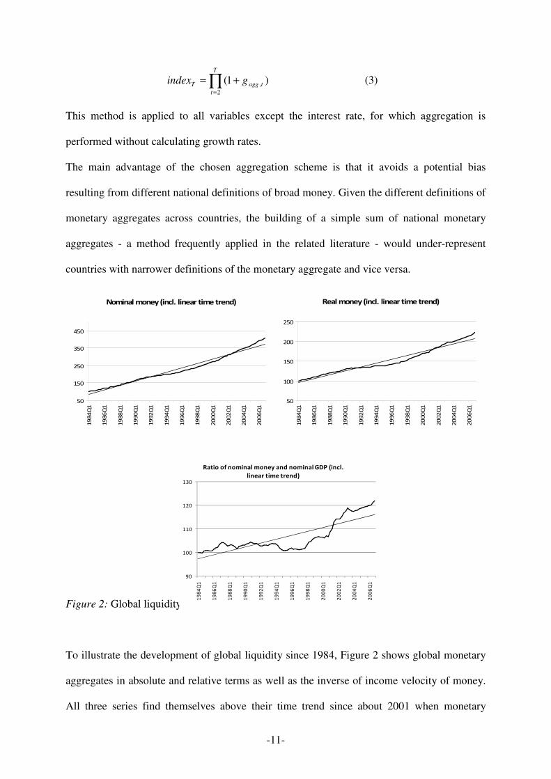
Figure 2: Global liquidity since 1984.

To illustrate the development of global liquidity since 1984, Figure 2 shows global monetary

aggregates in absolute and relative terms as well as the inverse of income velocity of money.

All three series find themselves above their time trend since about 2001 when monetary

Nominal money (incl. linear time trend)

50

150

250

350

450

1984Q1

1986Q1

1988Q1

1990Q1

1992Q1

1994Q1

1996Q1

1998Q1

2000Q1

2002Q1

2004Q1

2006Q1

Real money (incl. linear time trend)

50

100

150

200

250

1984Q1

1986Q1

1988Q1

1990Q1

1992Q1

1994Q1

1996Q1

1998Q1

2000Q1

2002Q1

2004Q1

2006Q1

90

100

110

120

130

1984Q1

1986Q1

1988Q1

1990Q1

1992Q1

1994Q1

1996Q1

1998Q1

2000Q1

2002Q1

2004Q1

2006Q1

Ratio of nominal money and nominal GDP (incl.

linear time trend)

-12-

policymakers turned to a more expansionary policy in the course of the rapid downturn in

stock markets and a number of further shocks such as September 11th. Money growth

remained strong throughout the last years, as indicated by the persistent growth of the ratio of

nominal money to nominal GDP – a measure frequently applied as an indicator of excess

liquidity.10

Overall, the graphical inspection provides some first glance for the view that

global liquidity is indeed at a high level and that the term excess liquidity can be justified

rather easily when analyzing the most recent period.

Figure 3 displays the remaining aggregated economic variables of interest. The GDP deflator

series clearly elucidates the moderate inflation which started to emerge around the mid-90s

and has persisted until 2006 although monetary aggregates expanded heavily in recent years.

Global short-term interest rates were at a historically low level from 2002 to 2005, since the

monetary policy stance was extremely loose during this period.11

Interestingly, the global time

series show that the recent years of global excess liquidity are accompanied by strong price

increases in both housing and commodity markets. The ongoing discussion about the linkage

of global excess liquidity and asset price inflation is not least based on this phenomenon. In

the following econometric analysis we will investigate the causal connection of global

liquidity and asset and commodity price inflation in a more formal framework.

10

See, for instance, Rüffer and Stracca (2006). 11

One might regard the deviation from an estimated Taylor rate as a more accurate measure in this respect.

However, these numbers create a rather similar picture. See International Monetary Fund (2007), Chapter 1, Box

1.4.

-13-

Figure 3: Global series of GDP deflator, short-term interest rate, real GDP, commodity prices

and house prices

4.2 The VAR Methodology

The econometric framework employed is a vectorautoregressive model (VAR) which allows

us to model the impact of monetary shocks on the economy while taking care of the feedback

between the variables since all of them are treated as endogenous.12

Based on the VAR

analysis, we apply impulse response analyses which provides insights into the short- and

long-run relationship of our variables of interest.

Consider first the traditional reduced-form VAR model:

ttt uCZYL +=Γ )(

(4)

12

Of course, one could model exogenous variables as well, but this option is not used here. One reason is that we

consider a world model, where there are no exogenous variables by definition. Moreover, from an econometric

point of view, we refer to our point estimates. They reveal that no variable is weakly exogenous. Instead, all

variables cannot be rejected to be endogenous.

-14-

where tY is the vector of the endogenous variables and )(LΓ is a matrix polynomial in the lag

operator L for which ip

i i LAIL ∑ =+=Γ

1)( , so that we have p lags. tZ is a matrix with

deterministic terms, C is the corresponding matrix of coefficients, and tu is the vector of the

white noise residuals where serial correlation is excluded, so that:

0)( =tuE (5)

≠

=Σ=

st

stuuE st

:0

:)( | (6)

Since Σ is not a diagonal matrix, contemporaneous correlation is allowed. In order to model

uncorrelated shocks, a transformation of the system is needed. Using the Cholesky

decomposition 'PP=Σ , taking the main diagonal of P to define the diagonal matrix D and

premultiplying (4) with 1: −=Ψ DP yields the structural VAR (SVAR) representation:

ttt eZCYLK +=*)( (7)

ip

i

i LALK ∑=

+Ψ=1

*)( (8)

The contemporaneous relations between the variables are now directly explained in Ψ , which

is a lower triangular matrix with all elements of the main diagonal being one. The innovations

te are by construction uncorrelated: ''''''')( 11|DDDPPPDPPPeeE tt ==ΨΨ=ΨΣΨ=

−− .

Similarly, the Cholesky decomposition is used to construct orthogonal innovations out of the

moving average representation of the system which is the cornerstone of the impulse response

analysis.

Furthermore, the use of the Cholesky decomposition implies a recursive identification scheme

which involves restrictions about the contemporaneous relations between the variables. The

latter are given by the (Cholesky) ordering of the variables and might considerably influence

the results of the analysis. Therefore, different orderings are used to prove the robustness of

our results.

-15-

Unit root tests indicate that all our series are integrated of order one. Thus the question arises

whether one should take differences of the variables in order to eliminate the stochastic trend.

However, Sims, Stock and Watson (1990) show that Ordinary Least Squares estimates of

VAR coefficients are consistent under a broad range of circumstances even if the variables are

nonstationary.13

Therefore, we strictly follow this approach and estimate the VAR model in

levels.

13

Estimating the VAR in levels does not pose any problems, if all variables are stationary (I(0)). If some

variables have a unit root (I(1)) and the series are not cointegrated, a VAR in levels or first differences makes no

difference asymptotically. Taking first differences only tends to be better in samples smaller than ours (Hamilton,

1994, pp. 553, 652). However, if two or more variables are I(1) and cointegrated, the first difference estimates

are biased if there is cointegration because the error-correction term is omitted. An alternative in the latter case

would be to estimate a VECM. However, since it is hard to identify with any degree of accuracy the underlying

structural parameters of a VECM which includes a large number of variables, for practical reasons we derive

impulse responses from a VAR in levels, which due to its simplicity seems to be a more appropriate technique.

-16-

4.3 Empirical findings

4.3.1 The baseline model

We are starting our VAR analysis by estimating a benchmark model which includes the

traditional macroeconomic variables output (GDP), GDP deflator (PGDP), short-term interest

rate (IS), and broad money (M). Further, we include the house (HPI) and the commodity price

index (COM) in our model in order to test for different price reaction of assets and goods to a

liquidity shock. In addition, a constant and a linear time trend are added. All variables are

taken in log-levels except the interest rate. Our benchmark specification is thus given by the

following vector of endogenous variables (along with the corresponding Cholesky ordering):

( , , , , , )t t

x GDP PGDP COM HPI M IS= (9)

The Cholesky ordering of the basic specification follows the principle that monetary variables

should be ordered last, since they are expected to react faster to the real economy than vice

versa (Favero, 2001). Within the monetary variables, we impose the restriction that money

does not react contemporaneously to interest rates which helps to interpret our liquidity shock

as a money supply shock.14

The price variables PGDP, COM and HPI are ordered in the

middle given that they are supposed to react to the monetary variables only with a lag. In

general, the results are very robust to changes in the ordering within the three blocks. To

determine lag length, we apply the usual criteria.15

Most of the criteria point at a lag length of

two, which is also sufficient to avoid serial correlation among the residuals and seems to be

appropriate in order to estimate a model which is parsimonious where possible.16

While this is

true not only for the benchmark specification but also for the following models we will

continue with two lags for the whole analysis.

14

For a money demand shock, interest rates should be ordered before money in order to enable economic agents

to adjust their money holdings immediately to changes in the opportunity costs of holding money. 15

To be explicit, we used the Likelihood Ratio test, the Final Prediction Error, the Akaike information criterion,

the Schwarz criterion and the Hannan-Quinn criterion. 16

To test for autocorrelation of the residuals, we performed the Lagrange Multiplier test.

-17-

Figure 4: Impulse response analysis for benchmark specification17

Figure 4 displays the impulse responses with respect to an unexpected increase in global

liquidity. (See the appendix for the whole array of impulse responses.) Referring to our

theoretical considerations outlined above (se Figure 1), it helps us to disentangle short-run

from longer-run elasticities. In particular for certain asset prices, but to a lower extent, also for

17

The confidence intervals of our impulse responses display two standard deviations and are calculated via the

studentized Hall bootstrap method.

-18-

consumer prices, the price elasticity of supply is time-varying, i.e. is low in the short run, but

increases over time (see Fig. 1). Short-run elasticities correspond with the estimated short-run

responses of the respective variable of interest, i.e. the different asset prices, to a global

liquidity shock. Accordingly, long-run elasticities are mirrored by the long-run responses.

Figure 4 has all features expected from our theoretical considerations: The GDP deflator

reacts slowly but moves upwards significantly after about eleven quarters. Thus, in our model

money matters for and causes goods price inflation although substantial time lags have to be

taken into account. Quicker positive responses to a global liquidity shock are given by the

house price and the commodity price index (after three and nine quarters respectively). From

a theoretical point of view, the lower price elasticity of supply in the housing and in the

commodity market compared to the goods market should contribute to this finding. Initially,

the spurt in demand will come up against an inelastic supply driving prices up sharply,

especially if the spurt in demand is unanticipated as it is in the VAR methodology used here.

This will provide the incentive for an increase in supply according to, say, a Tobin Q theory

of investment. This, in turn, could lead to over-supply and a collapsing asset price. So, the

money story that we are using can explain not just booming asset prices but also collapsing

asset prices.18

These results also provide some interesting interpretations for the post-2001 period.

Apparently, abundant global liquidity contributed to the bull market in the real estate sector.

Following the downturn in the housing market triggered by the subprime crisis, money

balances werethen flowing largely into commodity markets putting upward pressure on

commodity prices.

It is also of interest that commodity prices react later than house prices to a shock of global

liquidity. This is consistent with anecdotical evidence during the recent food price hike when

global demand, driven by “hunger for return”, turned to commodities after house prices had

18

We owe this point to an anonymous referee.

-19-

collapsed. On a more theoretical level, one could argue that house prices react faster than

commodity prices to an unexpected increase in liquidity since expectations of future

economic growth might be even more important for commodities than for real estate and, thus,

shocks to global liquidity only pour into commodity markets when economic growth

accelerates.19

Moreover, speculation may play a more important role in housing markets. If

assets can be stored, people expecting a price rise can take some amount off today’s market,

driving up the price now, in the expectation that they can sell it at a higher price later.

Commodities which are characterized by a lower degree of storability than housing, then

display less distinguished and slower price increases than housing (Krugman, 2008).

The remaining impulse responses of our benchmark model are also in line with economic

theory. The negative reaction of the interest rate to a liquidity shock is consistent with the

interpretation of our liquidity shock as a money supply shock. GDP moves up temporarily but

not permanently as a result of the liquidity shock, which is in line with the theoretical

assumption that money is neutral for the real economy in the long run. Interestingly, the price

puzzle (the absence of a decline of the price level due to a positive interest rate shock), which

is often found in similar VAR models, does not appear in our model (see Figure A1 in the

appendix). Note also that the response of our variables to an interest rate shock is very

consistent with the dynamic adjustment to a global liquidity shock. Moreover, since a

negative interest rate shock has similar consequences for house and consumer prices as a

positive liquidity shock, a pure money supply shock (a growing money stock accompanied by

a decreasing interest rate) should give even higher effects than our money-only shocks given

above. Further, it is of interest to see that house price shocks have predictive content for

future goods price inflation suggesting that house prices should be taken into account by

monetary authorities as they signal changes in expected goods price inflation (see Goodhart

and Hofmann 2007 for similar results).

19

Note the striking similarity in the impulse responses of a liquidity shock to output and to commodity prices.

-20-

4.3.2 Augmenting the VAR with stocks and gold

Given that the dynamics of the benchmark model is found to be plausible, the next step in our

VAR analysis is to augment our baseline model with further asset variables. Specifically, we

include the gold price (in US dollars) and, alternatively, a globally aggregated stock price

index in our model.20

Similar to house and commodity prices these time series are

characterized by significant upwards movements in recent years (Figure 5).

Figure 5: Gold and global stock prices.

Gold prices are of particular interest given that the actual amount of gold which can be

produced in any year is only a minor share of the stock of gold. Thus the increase in the

quantity of gold supplied in response to an aggregate demand shock is only a small fraction of

the stock of gold, resulting a in a very steep supply curve.

In the Cholesky ordering, we put gold just behind the house price index, given its assumed

sensitiveness to monetary policy shocks; however, results are again very robust to changes in

the ordering within the “price block”:

( , , , , , , )t t

x GDP PGDP COM HPI GOLD M IS= (10)

20

Note that the HWWI commodity price index does not include gold and thus there arise no problems of

multicollinearity. Data for stock prices are from Datastream. For each country in our sample we use the key

national stock market index and aggregate the series to a global index as described in section 4.1.

Stocks

100

400

700

1000

1300

1600

1984Q

1

1986Q

1

1988Q

1

1990Q

1

1992Q

1

1994Q

1

1996Q

1

1998Q

1

2000Q

1

2002Q

1

2004Q

1

2006Q

1

Gold

0

40

80

120

160

200

-21-

Figure 6: Impulse response analysis for model augmented with gold price.

Figure 6 displays the impulse responses of our extended model that are of main interest.

Global liquidity shocks again positively and significantly influence the price level for goods

and services (GDP deflator), housing and commodities. Interestingly, the response of the gold

price is even faster. Gold prices react significantly after three quarters to an unexpected

increase in global liquidity. This confirms our theoretical assumption that the price elasticity

of supply is decisive to what degree global liquidity shocks are reflected in the price level.

The quantity of gold cannot be easily extended so that the supply of gold is relatively price-

inelastic and the reaction speed of the gold price is therefore quicker compared to other asset

prices.

-22-

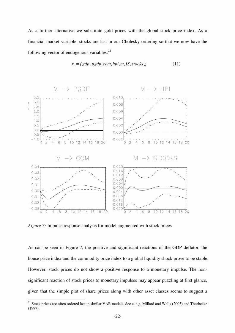
As a further alternative we substitute gold prices with the global stock price index. As a

financial market variable, stocks are last in our Cholesky ordering so that we now have the

following vector of endogenous variables:21

( , , , , , , )t t

x gdp pgdp com hpi m IS stocks= (11)

Figure 7: Impulse response analysis for model augmented with stock prices

As can be seen in Figure 7, the positive and significant reactions of the GDP deflator, the

house price index and the commodity price index to a global liquidity shock prove to be stable.

However, stock prices do not show a positive response to a monetary impulse. The non-

significant reaction of stock prices to monetary impulses may appear puzzling at first glance,

given that the simple plot of share prices along with other asset classes seems to suggest a

21

Stock prices are often ordered last in similar VAR models. See e, e.g, Millard and Wells (2003) and Thorbecke

(1997).

-23-

quite high correlation (Figures 3 and 5). However, a closer inspection of the time series also

reveals significant differences across asset classes. The empirical realisation of the coefficient

of variation calculated over our whole sample period amounts to 0.61 for stock prices but only

to 0.27 for house prices. The dot.com bubble and its burst are fully reflected in the stock price

time series whereas no such accentuated blip becomes obvious in the house price time series.

These observations are in line with the suggestion by many scholars that house prices tend to

move in long cycles whereas stock prices as a stylized fact can be best characterized as

random walks (see, for instance, Gros, 2007). Moreover, our result is consistent with

theoretical considerations according to which the relationship between money and stock

prices is less pronounced than for other asset classes (Deutsche Bundesbank, 2007, Fischer,

Lenza, Pill, and Reichlin, 2008). On the one hand, higher liquidity tends to increase

household’s assets, and a part of the associated wealth increase may be held in the form of

shares. On the other hand, high (expected) securities returns make the holding of shares more

attractive than holding money. This may trigger important substitution effects, i.e. shifts

between money and shares. As a result, the relationship between the developments in the

stock market and money holdings is not clear cut.22

4.4 Robustness checks

To check for the robustness of our results, we additionally estimated several alternative

versions of our model. First, we changed the lag lengths (especially 4 lags) with nearly no

consequences for our results. Second, we used different Cholesky orderings in order to avoid

that our results rely on any particular assumption regarding the structural equations of our

VAR model. No major changes in the results occurred.

22

The ambiguous relationship between money and stock prices is also reflected in the results of other empirical

studies. While Kontolemis (2002) finds a dominant substitution effect in the relationship between money and

stock prices, Bruggemann, Donati, and Warne (2003) obtain a prevalent wealth effect.

-24-

Figure 7: Impulse response analysis for sample period beginning in 1990 (first row) and 1995

(second row)

As a third robustness check, we restricted the sample to the period from 1990 and 1995 on,

respectively. This is motivated by the insight that the widespread capital account and trade

liberalization since 1990 should contribute to the different dynamics in the price-money

relationship. To overcome the problem of increasing estimation variability due to declining

degrees of freedom, we used just one lag for this analysis. As is revealed by Figure 7 the

results remain pretty stable and especially the main direction of the liquidity shocks is once

again confirmed. Thus, there is some evidence for the view that the different price

adjustments in consumer and asset prices to a liquidity shock are phenomena which are not

only related to the most recent period but exist throughout our observation period (although

they may be more apparent in recent years given the large expansion in liquidity in the post-

-25-

2001 period). Again, there is a significant transmission mechanism reaching from housing

markets to consumer markets. However, the results should be interpreted with care due to the

short sample period.

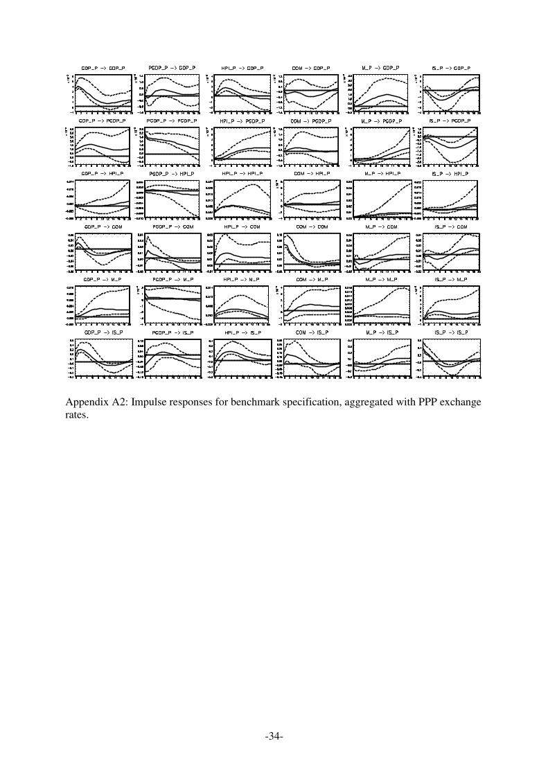
Fourth, we used an alternative aggregation scheme for our global aggregates in order to find

out if the results are sensible in this respect. As we used market exchange rates so far for the

calculation of the individual country weights we also checked for the alternative of using PPP

exchange rates in the aggregation procedure. (This results in a substitution in equation (1):

PPP

tie , instead of tie , ).23

Figure 8 displays selected impulse responses of our benchmark model

when using PPP aggregation. (See Appendix A2 for the full set of impulse responses.) The

main empirical findings are not affected. Global liquidity shocks again lead to a temporary

increase of the output variable and to a permanent and significant increase of the GDP

deflator, the house price index and the commodity price index. The high robustness of the

results to the aggregation scheme should not come as a surprise given that many variables in

our sample are highly correlated at an international level – a phenomenon which renders the

form of aggregation less important.

23

The base year for our PPP exchange rates is 1999.

-26-

Figure 8: Impulse response analysis for benchmark specification; aggregation with PPP

exchange rates

5. Conclusions

In this paper, we have analyzed the effects of global liquidity shocks on goods prices and a

variety of asset prices. We come up with the following empirical results: First, we find

support of the conjecture that monetary aggregates may convey useful leading indicator

information on variables such as house prices, gold prices, commodity prices and the GDP

deflator at the global level. In contrast, stock prices do not show any positive response to a

liquidity shock - a result which might be related to the relatively higher importance of

substitution effects for this asset class. Second, our VAR results support the view that

different price elasticities on asset and goods markets explain the recently observed relative

price change between asset classes and consumer goods. In line with theoretical reasoning,

-27-

the price reaction of asset prices takes place faster than that of goods prices. Third, we find

significant spill-over effects from housing markets to goods price inflation suggesting that a

forward-looking monetary policy has to take asset price developments into account. In sum,

we would therefore like to argue that global liquidity deserves at least the same attention as

the worldwide level of interest rates has received in the recent intensive debate on the world

savings versus liquidity glut hypothesis, if not possibly more.

Against the background of our results the still high level of global liquidity has to be

interpreted as a threat for future stable and low inflation and financial stability. Since global

excess liquidity is found to be an important determinant of asset and goods prices, there might

be at least three implications for the adequate conduct of monetary policy. First, monetary

policy has to be aware of different time lags in the transmission from liquidity to different

categories of prices. In particular, strong money growth might be a good indicator of

emerging future bubbles in the real estate sector and later on also of bubbles in gold and

commodity markets. However, it does not seem to be a good leading indicator for stock prices.

Second, this pattern should, on the contrary, also be taken into account when assessing the

consequences of a slowing down or smooth reversal in global excess liquidity - for instance,

the risks and options in the light of Bretton Woods II.

If it is indeed true that floating exchange rates no longer impart monetary autonomy to

national monetary policies, then this has serious implications for the future organization and

operation of monetary policy.24

If global liquidity plays a significant role within the

transmission mechanism on a global or on a national level, central banks almost certainly tend

to lose influence. From the perspective of central banks, this is a clear disadvantage of

globalization for monetary policy (up to now the discussion focused more on the advantages

as, for instance, the inflation curbing effects). For instance, the traditional interest rate channel

could be distorted in some countries. Imagine a central bank raises its policy rate in order to

24

We are grateful to an anonymous referee for calling our attention to this point.

-28-

fight inflationary pressures. Thereupon parts of global excess liquidity pour into the home

country in order to profit from the interest rate differential and counteract the restrictive

interest rate policy. A further research question raised by our paper is to what extent the

phenomenon of global excess liquidity makes a coordination of national monetary policies

useful (abstracting from practicability issues). Go-it-alone policies by national central banks

in order to prevent unsolicited effects of global excess liquidity on national variables

potentially evaporate.

If excess liquidity - as reflected by our orthogonal money shock variables - creates such huge

distortions in asset prices (severe misalignment) and in overall inflation, along with the severe

misallocation of resources that goes along with these, and arguably the global systemic

collapse we are currently undergoing, then either long-run neutrality of money is compatible

with huge real economic distortions in the wake of strong money expansion or it is even hard

to claim that money is neutral in the long run (as we find in the impulse response analysis),

unless this long run is chronologically so far in the future that it becomes irrelevant to any

policy consideration. However, this is a more general issue, not unique to our paper and,

hence, left to further research.

References

Adalid, R., Detken, C., 2007. Liquidity Shocks and Asset Price Boom/Bust Cycles. ECB

Working Paper Series 732, Frankfurt a. M.

Baks, K., Kramer, C. F., 1999. Global Liquidity and Asset Prices: Measurement, Implications,

and Spillovers. IMF Working Papers 99/168, Washington, D.C.

Belke, A., Gros, D., 2007. Instability of the Eurozone? On Monetary Policy, House Prices and

Labor Market Reforms. IZA Discussion Papers 2547, Bonn.

-29-

Beyer, A., Doornik, J.A., Hendry, D.F., 2000. Constructing Historical Euro-Zone Data.

Economic Journal 111, 308-327.

Borio, C. E. V., Filardo, A., 2007. Globalisation and Inflation: New Cross-Country Evidence

on the Global Determinants of Domestic Inflation. BIS Working Papers 227, Basle.

Browne, F., Cronin, D. 2007. Commodity Prices, Money and Inflation. ECB Working Paper

738, European Central Bank, Frankfurt a. M.

Brunnermeier, M.K., Nagel, S., Pedersen, L.H., 2008. Carry Trades and Currency Crashes.

NBER Working Paper 14473, National Bureau of Economic Research, Cambridge/MA,.

Bruggemann, A., Donati, P., Warne, A. (2003). Is the Demand for Euro Area M3 Stable?,

ECB Working Paper 255, European Central Bank, Frankfurt a. M.

Canova, F., Ciccarelli, M., Ortega, E., 2007. Similarities and Convergence in G-7 Cycles.

Journal of Monetary Economics 54 (3), 850-878.

Ciccarelli, M., Mojon, B., 2005. Global Inflation. ECB Working Paper 537, Frankfurt a.M.

Congdon, T., 2005. Money and Asset Prices in Boom and Bust. The Institute of Economic

Affairs, London.

Deutsche Bundesbank, 2007. The Relationship Between Monetary Developments and the

Real Estate Market. Monthly Report, July, 13-24.

Del Negro, M., Otrok, C., 2007. 99 Luftballons: Monetary Policy and the House Price Boom

across US States. Journal of Monetary Economics 54 (7), 1962-1985.

Favero, C. A., 2001. Applied Macroeconometrics. Oxford University Press, New York.

Fischer, B., Lenza, M., Pill, H., Reichlin, L., 2008. Money and Monetary policy: the ECB

Experience 1999-2006. In Beyer, A., Reichlin L. (eds)..The Role of Money: Money and

Monetary Policy in the Twenty-First Century. Conference Volume of the 4th ECB Central

Bank Conference, 102-175.

-30-

Giese, J. V.,Tuxen, C. K., 2007. Global Liquidity, Asset Prices and Monetary Policy:

Evidence from Cointegrated VAR Models. Unpublished Working Paper. University of

Oxford, Nuffield College and University of Copenhagen, Department of Economics.

Giuliodori, M., 2005. The Role of House Prices in the Monetary Transmission Mechanism

Across European Countries. Scottish Journal of Political Economy 52 (4), 519-543.

Goodhart, C. A. E., Hofmann, B., 2001. Asset Prices, Financial Conditions, and the

Transmission of Monetary Policy. Federal Reserve Bank of Kansas City Proceedings, March.

Goodhart, C. A. E., Hofmann, B., 2007. House Prices and the Macroeconomy: Implications

for Banking and Price Stability. Oxford University Press, Oxford.

Greiber, C., Setzer, R., 2007. Money and Housing: Evidence for the Euro Area and the US.

Deutsche Bundesbank Discussion Paper Series 1: Economic Studies 07/12, Frankfurt a. M.

Gros, D. (2007): Bubbles in Real Estate? A Longer-Term Comparative Analysis of Housing

Prices in Europe and the US, CEPS Working Document No. 276, October, Brussels.

Hamilton, J. D. 1994, Time Series Analysis, Princeton University Press, Princeton, NJ.

Krugman, P., 2008. Commodity Prices (Wonkish), New York Times, March 19th

.

Kontolemis, Z. 2002. Money Demand in the Euro Area: Where Do We Stand (Today)?.

International Monetary Fund, IMF Working Paper, No. 185.

Iacoviello, M., 2005. House Prices, Borrowing Constraints, and Monetary Policy in the

Business Cycle. American Economic Review 95 (3), 739-764.

International Monetary Fund, 2004. The Global House Price Boom, in: World Economic

Outlook - The Global Demographic Transition, Chapter II, pp. 71-89. September 2004,

Washington, D.C.

International Monetary Fund, 2007. What is Global Liquidity?, in: World Economic Outlook

- Globalization and Inequality, Chapter I, pp. 34-37. October 2007, Washington, D.C.

-31-

Jylhä, P., Suominen, M. and Lyytinen, J.-P., 2009. Arbitrage Capital and Currency Carry

Trade Returns. Paper presented at the American Finance Association (AFA) Conference,

January 3-5, San Francisco.

Miles, M.A., 1978. Currency Substitution, Flexible Exchange Rates, and Monetary

Independence. American Economic Review 68, 428-436.

Millard, S. P., Wells, S. J.,2003. The Role of Asset Prices in Transmitting Monetary and other

Shocks. BoE Working Papers 188, Bank of England, London.

Mishkin, F. S., 2007. Housing and the Monetary Transmission Mechanism. NBER Working

Paper 13518.

OECD, 2005. Recent House Price Developments: The Role of Fundamentals, in: OECD

Economic Outlook 78, Chapter III, pp. 193-234.

Papademos, L., 2007. The Effects of Globalisation on Inflation, Liquidity and Monetary

Policy. Speech at the conference on the ”International Dimensions of Monetary Policy”

organised by the National Bureau of Economic Research, S’Agar`o, Girona, June 11th 2007.

Pepper, G. with Olivier, M., 2006. The Liquidity Theory of Asset Prices. Wiley Finance.

Plantin, G., Shin, H.S., 2008. Carry Trades and Speculative Dynamics. Available at SSRN:

http://ssrn.com/abstract=898412, February.

Reinhart, C. M., Rogoff, K. S., 2004. The Modern History of Exchange Rate Arrangements:

A Reinterpretation. Quarterly Journal of Economics 119 (1), 1-48.

Roffia, B., Zaghini, A., 2007. Excess Money Growth and Inflation Dynamics. ECB Working

Paper 749, Frankfurt a. M.

Rueffer, R., Stracca, L., 2006. What Is Global Excess Liquidity, and Does It Matter? ECB

Working Paper 696, Frankfurt a. M.

De Santis, R. A., Favero, C., Roffia, B., 2008. Euro Area Money Demand and International

Portfolio Allocation. ECB Working Paper 926, Frankfurt a. M.

-32-

Schich, S., Weth, M., 2008. Demographic Changes and Real House Prices. Forthcoming.

Deutsche Bundesbank, Frankfurt a. M.

Schnabl, G., Hoffmann, A. 2007. Monetary Policy, Vagabonding Liquidity and Bursting

Bubbles in New and Emerging Markets – An Overinvestment View. CESifo Working Paper

2100, Munich.

Shiller, R., 2005. Irrational Exuberance. 2nd edition. Princeton University Press, New Jersey.

Sims, C. A., Stock, J. H., Watson, M. W., 1990. Inference in Linear Time Series Models with

Some Unit Roots. Econometrica 58 (1), 113-144.

Sousa, J. M., Zaghini, A., 2006. Global Monetary Policy Shocks in the G5: A SVAR

Approach. CFS Working Paper 2006/30, Frankfurt a. M.

Taylor, M., 2000. Purchasing Power Parity Over Two Centuries: Strengthening the Case for

Real Exchange Rate Stability, Journal of International Money and Finance, 19, 759-64.

Thorbecke, W., 1997. On Stock Market Returns and Monetary Policy. Journal of Finance 52

(2), 635–654.

-33-

Appendix

Appendix A1: Impulse responses for benchmark specification, aggregated with market

exchange rates.

-34-

Appendix A2: Impulse responses for benchmark specification, aggregated with PPP exchange

rates.