liquid phase ion mobility spectrometry - … · throughout my student life: ... liquid phase ion...

LIQUID PHASE ION MOBILITY SPECTROMETRY

By MAGGIE TAM

A dissertation submitted in partial fulfillment of the requirements for the degree of

DOCTOR OF PHILOSOPHY

WASHINGTON STATE UNIVERSITY Department of Chemistry

DECEMBER 2006

© Copyright by MAGGIE TAM, 2006 All Rights Reserved

ii

To the Faculty of Washington State University:

The members of the Committee appointed to examine the dissertation

of MAGGIE TAM find it satisfactory and recommend that it be accepted.

_________________________________

Chair

_________________________________

_________________________________

iii

Acknowledgement

I would like to thank Dr. Herbert H. Hill, Jr. for his continuous motivation and support

throughout my graduate study, and for his teachings and inspiration. He provided me

with opportunities to present at international conferences and to work on interesting

projects.

I would like to thank my committee: Dr. William F. Siems and Dr. James O. Schenk

for their guidance over the years. I would like to thank Dr. Siems for offering me the

valuable opportunity to work in the mass spectrometry core facilities, and for

teaching me the art and logic of troubleshooting. I would like to thank past and

present members from the Hill Research Group, especially Dr. Laura M. Matz and

Dr. Brian H. Clowers. Most sincere gratitude to Dr. Prabha Dwivedi for helping me

through trying times. I would like to thank my colleagues at LBB2 for sharing their

knowledge and experiences: Dr. Stephen Halls, Dr. Gerhard Munske, Dr. Xiaoting

Tang, Lisa Washburn, and Dr. Si Wu.

I would like to thank the professional staff in the WSU Chemistry Department for

their administrative support: Paula Broemmeling, Carrie Giovannini, Debbie

Arrasmith, Marie Martin, Nikki Clark, Roger Crawford, and Gary Johnson. I would

like to acknowledge the assistance from the staff of WSU Technical Services:

George Henry, Lauren Frei, Fred Schuetze, John Rutherford, Duke Beattie, and

Steve Watson, for their immense patience, expertise, and help on instrumental and

electrical problems. I would like to thank the WSU Research Foundation, especially

Dr. Brian Kraft, for the patent application.

iv

I would like to thank our collaborators, Dr. Amy Moll from Boise State University, Dr.

Prashanta Dutta from Washington State University, and their students, for

broadening my research experiences.

I would like to acknowledge financial support from the National Institute of Health

(NIBIB) and the Army Research Office for funding the thesis project, the WSU

Chemistry Department and Laboratory for Biotechnology and Bioanalysis, Unit 2, for

the TA positions. I would like to show appreciation for the Stacey Research

Scholarship, Jim and Lee Ruck Fellowship, and Don Matteson Fellowship, awarded

by the WSU Chemistry Department.

I would like to thank my WSU friends for providing me with lots of encouragement,

comfort, and laughter, especially Yan Liu, Wei Liao, Geoffrey and Adeline Puzon.

Most important of all, I would like to thank my family for their encouragement

throughout my student life: the Tam Family and the Chen family, my daughter

Audrey for bringing sunshine to my life, and my husband Jack for his confidence,

understanding, and support.

v

LIQUID PHASE ION MOBILITY SPECTROMETRY

Abstract

by Maggie Tam, Ph.D.

Washington State University

December 2006

Chair: Herbert H. Hill, Jr.

Liquid phase ion mobility spectrometry was developed as a novel analytical

separation method, by replacing the drift gas with a non-electrolyte containing

liquids. Preliminary studies demonstrated that liquid phase ion mobility spectrometry

was achievable. A miniaturized liquid phase ion mobility spectrometer obtained a

similar resolving power as a gas phase ion mobility spectrometer ten times its size.

A new ionization source, called electrodispersion ionization, was introduced. The

non-radioactive electrodispersion ionization source produced liquid phase ions in

non-electrolytic liquid medium. Visualization of the electrodispersion ionization

process showed electrodispersed droplets of aqueous sample. Exploration of the

sample flow rate established the pulsing controllability of electrodispersion ionization.

Pulsed electrodispersion ionization source was developed and evaluated for liquid

phase ion mobility spectrometry. Results demonstrated the capability of pulsed

electrodispersion ionization as a multipurpose ionization source for liquid phase ion

vi

mobility spectrometry, merging three important instrumental processes into a single

source: sample introduction, sample ionization, and pulsed ion injection.

vii

Table of Contents

Acknowledgement....................................................................................................... iii

Abstract ........................................................................................................................v

List of Tables...............................................................................................................xi

List of Figures............................................................................................................. xii

Chapter One: Introduction ......................................................................................... 1

History of ion mobility in liquid phase ................................................................. 1

Gas Phase Ion Mobility as an Analytical Separation Tool.................................. 4

Liquid Phase Ion Mobility as an Analytical Separation Tool............................... 9

Specific Aims .................................................................................................... 12

Attribution ......................................................................................................... 13

References ....................................................................................................... 14

Chapter Two: Electrodispersion Ionization in Liquids.............................................. 18

Abstract ............................................................................................................ 18

Introduction....................................................................................................... 19

Experimental Section........................................................................................ 22

Results and Discussions .................................................................................. 26

Conclusions ...................................................................................................... 32

Acknowledgements .......................................................................................... 33

viii

References ....................................................................................................... 34

Chapter Three: Liquid Phase Ion Mobility Spectrometry......................................... 51

Abstract ............................................................................................................ 51

Introduction....................................................................................................... 52

Experimental Section........................................................................................ 57

Results and Discussions .................................................................................. 62

Conclusions ...................................................................................................... 67


References ....................................................................................................... 68

Chapter Four: Design, Construction, and Evaluation of an Integrated Liquid Phase

Ion Mobility Spectrometer ......................................................................................... 83

Abstract ............................................................................................................ 83

Introduction....................................................................................................... 84

Design and Fabrication of Integrated Liquid Phase Ion Mobility Spectrometer 88

Results and Discussion .................................................................................... 92


References ....................................................................................................... 99

Chapter Five: Evaluation of Pulsed Electrodispersion Ionization Source for Liquid

Phase Ion Mobility Spectrometry ............................................................................ 109

Abstract .......................................................................................................... 109

ix

Introduction..................................................................................................... 110

Experimental Section...................................................................................... 112

Results and Discussion .................................................................................. 115

Conclusions .................................................................................................... 119

Acknowledgements ........................................................................................ 120

References ..................................................................................................... 121

Chapter Six: Conclusions ...................................................................................... 138

Appendix I: Additional Data from Parametric Studies of Electrodispersion Ionization

................................................................................................................................ 145

Appendix II: Additional Graphic Representations of Liquid Phase Ion Mobility

Spectrometers......................................................................................................... 152

Appendix III: Electric Circuit for Pulsed Electrodispersion Ionization Source ....... 167

Appendix IV: Secondary Electrospray Ionization-Ion Mobility Spectrometry for

Explosive Vapor Detection...................................................................................... 171

Abstract .......................................................................................................... 171

Introduction..................................................................................................... 173

Experimental Section...................................................................................... 175

Results And Discussion.................................................................................. 178

Conclusions .................................................................................................... 186

Acknowledgement .......................................................................................... 186

x

References ..................................................................................................... 187

xi

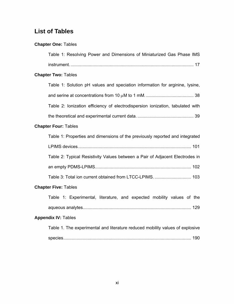
List of Tables

Chapter One: Tables

Table 1: Resolving Power and Dimensions of Miniaturized Gas Phase IMS

instrument. ..................................................................................................... 17

Chapter Two: Tables

Table 1: Solution pH values and speciation information for arginine, lysine,

and serine at concentrations from 10 μM to 1 mM. ....................................... 38

Table 2: Ionization efficiency of electrodispersion ionization, tabulated with

the theoretical and experimental current data. .............................................. 39

Chapter Four: Tables

Table 1: Properties and dimensions of the previously reported and integrated

LPIMS devices............................................................................................. 101

Table 2: Typical Resistivity Values between a Pair of Adjacent Electrodes in

an empty PDMS-LPIMS............................................................................... 102

Table 3: Total ion current obtained from LTCC-LPIMS. .............................. 103

Chapter Five: Tables

Table 1: Experimental, literature, and expected mobility values of the

aqueous analytes......................................................................................... 129

Appendix IV: Tables

Table 1. The experimental and literature reduced mobility values of explosive

species......................................................................................................... 190

xii

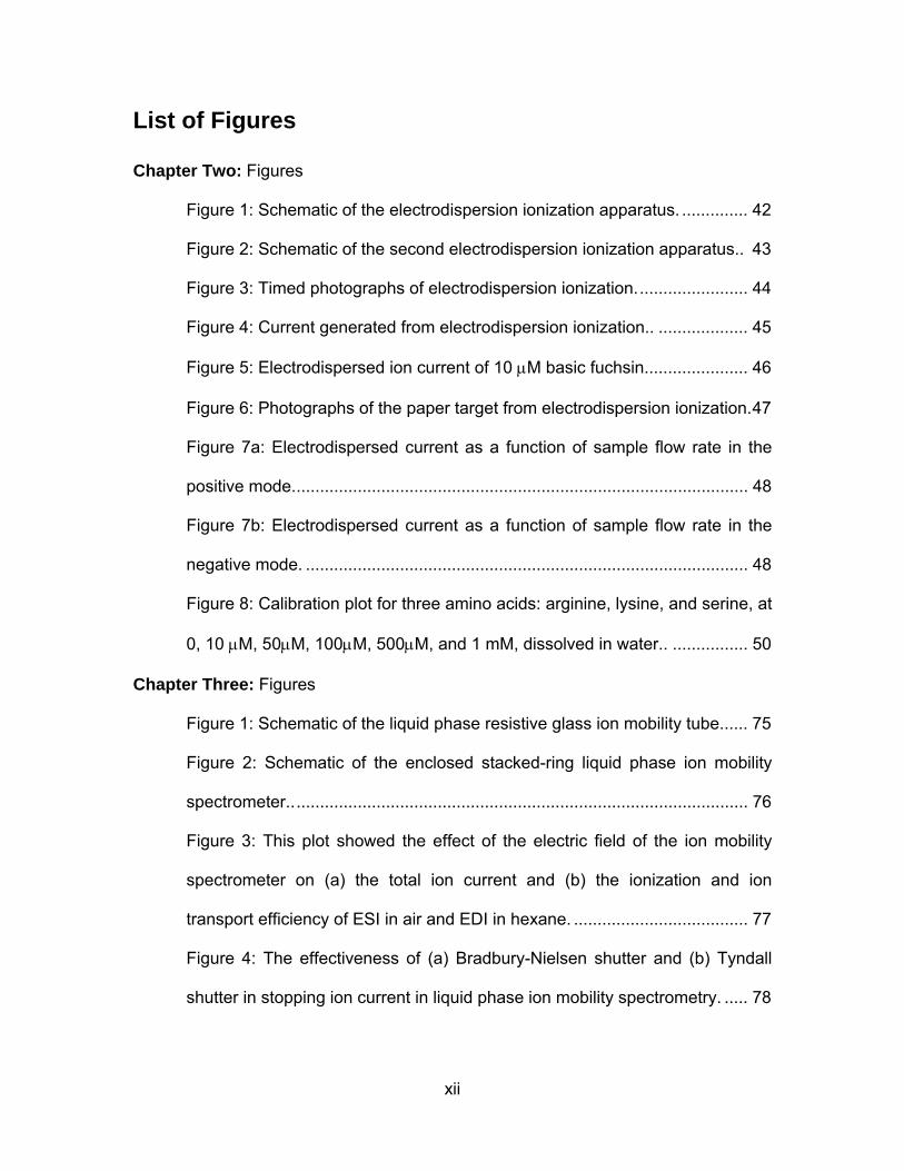
List of Figures

Chapter Two: Figures

Figure 1: Schematic of the electrodispersion ionization apparatus. .............. 42

Figure 2: Schematic of the second electrodispersion ionization apparatus.. 43

Figure 3: Timed photographs of electrodispersion ionization........................ 44

Figure 4: Current generated from electrodispersion ionization.. ................... 45

Figure 5: Electrodispersed ion current of 10 μM basic fuchsin...................... 46

Figure 6: Photographs of the paper target from electrodispersion ionization.47

Figure 7a: Electrodispersed current as a function of sample flow rate in the

positive mode................................................................................................. 48

Figure 7b: Electrodispersed current as a function of sample flow rate in the

negative mode. .............................................................................................. 48

Figure 8: Calibration plot for three amino acids: arginine, lysine, and serine, at

0, 10 μM, 50μM, 100μM, 500μM, and 1 mM, dissolved in water.. ................ 50

Chapter Three: Figures

Figure 1: Schematic of the liquid phase resistive glass ion mobility tube...... 75

Figure 2: Schematic of the enclosed stacked-ring liquid phase ion mobility

spectrometer.................................................................................................. 76

Figure 3: This plot showed the effect of the electric field of the ion mobility

spectrometer on (a) the total ion current and (b) the ionization and ion

transport efficiency of ESI in air and EDI in hexane. ..................................... 77

Figure 4: The effectiveness of (a) Bradbury-Nielsen shutter and (b) Tyndall

shutter in stopping ion current in liquid phase ion mobility spectrometry. ..... 78

xiii

Figure 5: Ion current of solvent blank, 10 μM basic fuchsin, and 1 μM

tetraethylammonium bromide. ....................................................................... 79

Figure 6: LPIMS spectra in mineral oil........................................................... 80

Figure 7: LPIMS spectra in mineral oil........................................................... 81

Figure 8: Pulsed electrodispersion ionization-liquid mobility spectrum of 10

μM basic fuchsin, dissolved in methanol-water (90:10, v/v), drifting in hexane.

....................................................................................................................... 82

Chapter Four: Figures

Figure 1: Schematic of the LTCC-LPIMS. ................................................... 105

Figure 2: (a) Top-view schematic of the third generation of PDMS-LPIMS

prototype. (b) Close-up three-dimensional view and (c) top-view of the sample

nozzle.. ........................................................................................................ 106

Figure 3: The surface methyl groups of poly(dimethylsiloxane) are oxidized to

hydroxyl group by oxygen plasma. .............................................................. 107

Figure 4: Plot of total ion current being measured at successive electrodes

along the PDMS channel in benzene.. ........................................................ 108

Chapter Five: Figures

Figure 1: Schematic of liquid phase ion mobility spectrometer (LPIMS) with

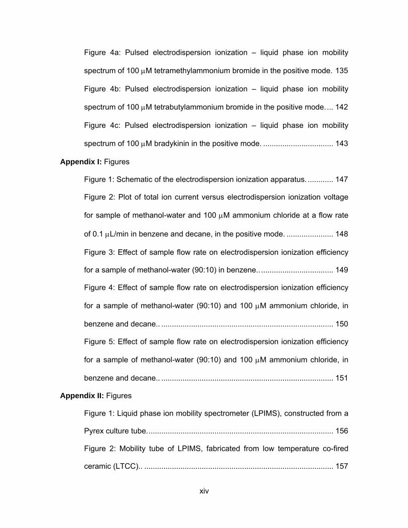
pulsed electrodispersion ionization (EDI). ................................................... 132

Figure 2: Pulsed electrodispersion ionization – liquid phase ion mobility

spectra of the solvent blank (methanol-water, 90:10 vol/vol) f. ................... 133

Figure 3: Pulsed electrodispersion ionization – liquid phase ion mobility

spectra of the solvent blank (methanol-water, 90:10 vol/vol) was obtained

over 30 minutes (179 spectra) in the positive mode.................................... 134

xiv

Figure 4a: Pulsed electrodispersion ionization – liquid phase ion mobility

spectrum of 100 μM tetramethylammonium bromide in the positive mode. 135

Figure 4b: Pulsed electrodispersion ionization – liquid phase ion mobility

spectrum of 100 μM tetrabutylammonium bromide in the positive mode.... 142

Figure 4c: Pulsed electrodispersion ionization – liquid phase ion mobility

spectrum of 100 μM bradykinin in the positive mode. ................................. 143

Appendix I: Figures

Figure 1: Schematic of the electrodispersion ionization apparatus. ............ 147

Figure 2: Plot of total ion current versus electrodispersion ionization voltage

for sample of methanol-water and 100 μM ammonium chloride at a flow rate

of 0.1 μL/min in benzene and decane, in the positive mode. ...................... 148

Figure 3: Effect of sample flow rate on electrodispersion ionization efficiency

for a sample of methanol-water (90:10) in benzene.................................... 149


for a sample of methanol-water (90:10) and 100 μM ammonium chloride, in

benzene and decane.. ................................................................................. 150


for a sample of methanol-water (90:10) and 100 μM ammonium chloride, in

benzene and decane.. ................................................................................. 151

Appendix II: Figures

Figure 1: Liquid phase ion mobility spectrometer (LPIMS), constructed from a

Pyrex culture tube........................................................................................ 156

Figure 2: Mobility tube of LPIMS, fabricated from low temperature co-fired

ceramic (LTCC).. ......................................................................................... 157

xv

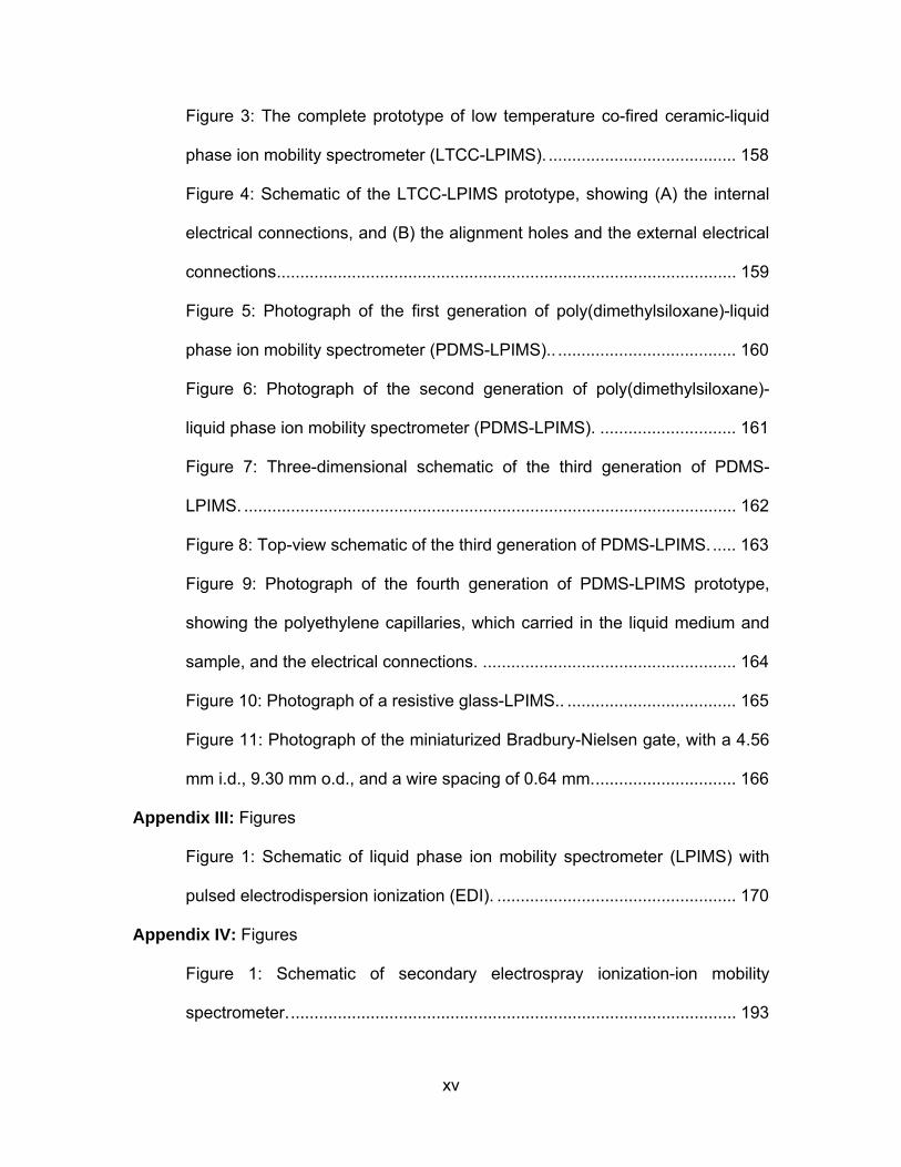
Figure 3: The complete prototype of low temperature co-fired ceramic-liquid

phase ion mobility spectrometer (LTCC-LPIMS). ........................................ 158

Figure 4: Schematic of the LTCC-LPIMS prototype, showing (A) the internal

electrical connections, and (B) the alignment holes and the external electrical

connections.................................................................................................. 159

Figure 5: Photograph of the first generation of poly(dimethylsiloxane)-liquid

phase ion mobility spectrometer (PDMS-LPIMS).. ...................................... 160

Figure 6: Photograph of the second generation of poly(dimethylsiloxane)-

liquid phase ion mobility spectrometer (PDMS-LPIMS). ............................. 161

Figure 7: Three-dimensional schematic of the third generation of PDMS-

LPIMS. ......................................................................................................... 162

Figure 8: Top-view schematic of the third generation of PDMS-LPIMS. ..... 163

Figure 9: Photograph of the fourth generation of PDMS-LPIMS prototype,

showing the polyethylene capillaries, which carried in the liquid medium and

sample, and the electrical connections. ...................................................... 164

Figure 10: Photograph of a resistive glass-LPIMS.. .................................... 165

Figure 11: Photograph of the miniaturized Bradbury-Nielsen gate, with a 4.56

mm i.d., 9.30 mm o.d., and a wire spacing of 0.64 mm............................... 166

Appendix III: Figures

Figure 1: Schematic of liquid phase ion mobility spectrometer (LPIMS) with

pulsed electrodispersion ionization (EDI). ................................................... 170

Appendix IV: Figures

Figure 1: Schematic of secondary electrospray ionization-ion mobility

spectrometer................................................................................................ 193

xvi

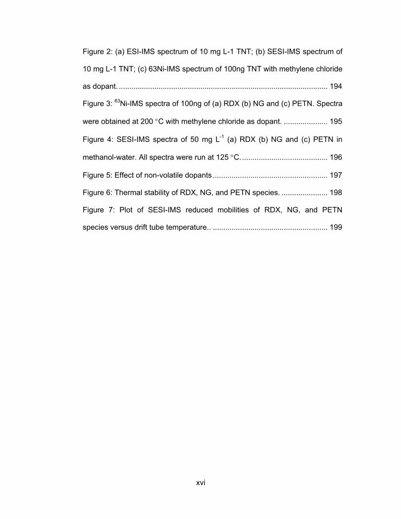
Figure 2: (a) ESI-IMS spectrum of 10 mg L-1 TNT; (b) SESI-IMS spectrum of

10 mg L-1 TNT; (c) 63Ni-IMS spectrum of 100ng TNT with methylene chloride

as dopant. .................................................................................................... 194

Figure 3: 63Ni-IMS spectra of 100ng of (a) RDX (b) NG and (c) PETN. Spectra

were obtained at 200 °C with methylene chloride as dopant. ..................... 195

Figure 4: SESI-IMS spectra of 50 mg L-1 (a) RDX (b) NG and (c) PETN in

methanol-water. All spectra were run at 125 °C.......................................... 196

Figure 5: Effect of non-volatile dopants ....................................................... 197

Figure 6: Thermal stability of RDX, NG, and PETN species. ...................... 198

Figure 7: Plot of SESI-IMS reduced mobilities of RDX, NG, and PETN

species versus drift tube temperature.. ....................................................... 199

1

Chapter One

Introduction

This project proposed to explore ion mobility in liquid phases as a novel analytical

separation technique in a miniaturized setting. Liquid phase ion mobility

spectrometry (LPIMS) separates analyte ions in an electric field established, not by

electrolyte, but by a series of metal electrodes held at decreasing potentials. The

development of a miniaturized LPIMS will have broad impact in separation sciences,

providing real-time separation of complex mixtures in the liquid phase.

History of ion mobility in liquid phase

Research of ion mobility in liquid phases began in the early 20th century as a series

of physical experiments evolving from conductivity studies of dielectric liquids. The

liquid media studied were liquid hydrocarbons, insulating oils and liquefied noble

gases.

Bialobrzeski and Jaffé conducted the first experiments of mobility measurements in

dielectric liquids in the early 20th century. Bialobrzeski [1] worked on the relation

2

between ion mobility and the viscosity (η) of the dielectric liquid medium and Jaffé [2]

performed ion mobility experiments in hexane. In 1937, Adamczewski [3] performed

the first systematic ion mobility experiments in a series of liquid saturated

hydrocarbons (pentane, hexane, heptane, octane and nonane) and studied the

relation of ion mobility to the coefficient of viscosity. Adamczewski concluded that the

mobility (μ) of ion was inversely proportional to η3/2 at constant temperature, known

as the Adamczewski’s relation:

-3/2μ = Aη (1)

where A is a numerical coefficient characteristic of each type of ions.

In the 1950s, measurements of mobility of helium ions in liquefied helium were done

by Williams [4], L. Meyer et al [5], Careri et al [6] and Atkins [7]. In 1964, Gzowski [8]

measured mobility of positive and negative ions in pure and mixtures of

hydrocarbons. Although the ions were not identified, he concluded that (1) positive

ions of different mobilities were present; (2) mobility of negative ions were greater

that that of positive ions in all the liquids studied; (3) mobility of negative ions were

found to be inversely proportional to viscosity of liquid, known as the Walden’s Rule:

-1μ = Aη (2)

and (4) mobility of positive ions were found to be inversely proportional to η3/2, same

as Adamczewski’s finding in 1937.

3

Adamczewski carried out more physical experiments on ion mobility in saturated

hydrocarbons [9] and formulated a relation between ion mobility and the number of

carbon atoms in the molecules of saturated hydrocarbons CnH2n+2 [10]:

( )1 21 2450- × n +2.33 n-1 -1.25

(0.45n) Tμ= 96e e⎧ ⎫⎡ ⎤⎨ ⎬⎢ ⎥⎣ ⎦⎩ ⎭ (3)

Interests in mobility studies in dielectric liquids continued, mostly used for physical

investigations of positive and negative intrinsic ions of the liquids in the study of the

breakdown process of dielectric liquids [11-13], the study of ion recombination and

diffusion in liquids subjected to high-energy radiation [14;15], and the study of

dielectric liquid properties in particle counters and spark chambers [16;17].

Investigations of ions from extrinsic analyte were less studied. Researchers studied

the mobilities of sulfur hexafluoride [18], methyl halides [18],

tetramethylparaphenylenediamine [19;20], quinones [20;21], porphines [20;21], and

fullerenes [20;22], with the samples dissolved in the same dielectric liquid medium

where experiments were conducted.

Up to this date, there has been no research performed on using ion mobility

spectrometry in liquid phases as an analytical separation technique for aqueous

phase analytes.

4

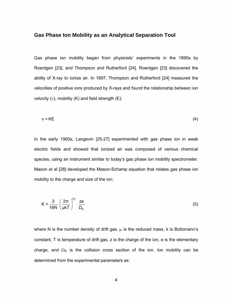
Gas Phase Ion Mobility as an Analytical Separation Tool

Gas phase ion mobility began from physicists’ experiments in the 1890s by

Roentgen [23], and Thompson and Rutherford [24]. Roentgen [23] discovered the

ability of X-ray to ionize air. In 1897, Thompson and Rutherford [24] measured the

velocities of positive ions produced by X-rays and found the relationship between ion

velocity (ν), mobility (K) and field strength (E):

ν = KE (4)

In the early 1900s, Langevin [25-27] experimented with gas phase ion in weak

electric fields and showed that ionized air was composed of various chemical

species, using an instrument similar to today’s gas phase ion mobility spectrometer.

Mason et al [28] developed the Mason-Schamp equation that relates gas phase ion

mobility to the charge and size of the ion:

1 2

D

3 2π zeK =16N μkT Ω

⎛ ⎞⋅ ⋅⎜ ⎟⎝ ⎠

(5)

where N is the number density of drift gas, μ is the reduced mass, k is Boltzmann’s

constant, T is temperature of drift gas, z is the charge of the ion, e is the elementary

charge, and ΩD is the collision cross section of the ion. Ion mobility can be

determined from the experimental parameters as:

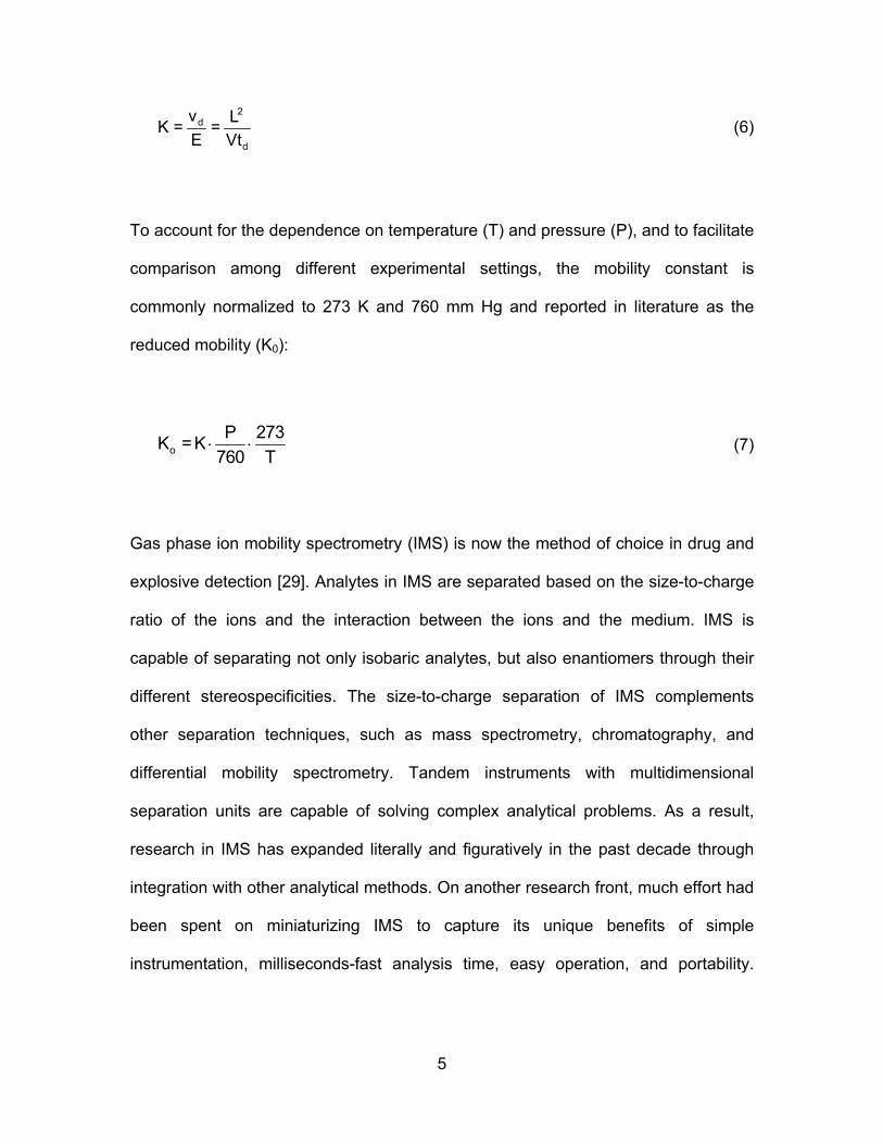
5

2d

d

v LK = =E Vt

(6)

To account for the dependence on temperature (T) and pressure (P), and to facilitate

comparison among different experimental settings, the mobility constant is

commonly normalized to 273 K and 760 mm Hg and reported in literature as the

reduced mobility (K0):

oP 273K =K

760 T⋅ ⋅ (7)

Gas phase ion mobility spectrometry (IMS) is now the method of choice in drug and

explosive detection [29]. Analytes in IMS are separated based on the size-to-charge

ratio of the ions and the interaction between the ions and the medium. IMS is

capable of separating not only isobaric analytes, but also enantiomers through their

different stereospecificities. The size-to-charge separation of IMS complements

other separation techniques, such as mass spectrometry, chromatography, and

differential mobility spectrometry. Tandem instruments with multidimensional

separation units are capable of solving complex analytical problems. As a result,

research in IMS has expanded literally and figuratively in the past decade through

integration with other analytical methods. On another research front, much effort had

been spent on miniaturizing IMS to capture its unique benefits of simple

instrumentation, milliseconds-fast analysis time, easy operation, and portability.

6

Portable IMS devices are widely employed by first responders for the rapid detection

of explosives and warfare agents.

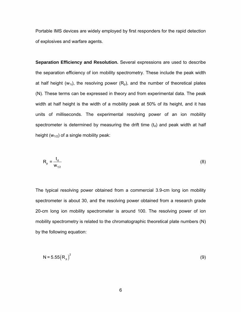
Separation Efficiency and Resolution. Several expressions are used to describe

the separation efficiency of ion mobility spectrometry. These include the peak width

at half height (w½), the resolving power (Rp), and the number of theoretical plates

(N). These terms can be expressed in theory and from experimental data. The peak

width at half height is the width of a mobility peak at 50% of its height, and it has

units of milliseconds. The experimental resolving power of an ion mobility

spectrometer is determined by measuring the drift time (td) and peak width at half

height (w1/2) of a single mobility peak:

dp

1 2

tR =

w (8)

The typical resolving power obtained from a commercial 3.9-cm long ion mobility

spectrometer is about 30, and the resolving power obtained from a research grade

20-cm long ion mobility spectrometer is around 100. The resolving power of ion

mobility spectrometry is related to the chromatographic theoretical plate numbers (N)

by the following equation:

( )2pN = 5.55 R (9)

7

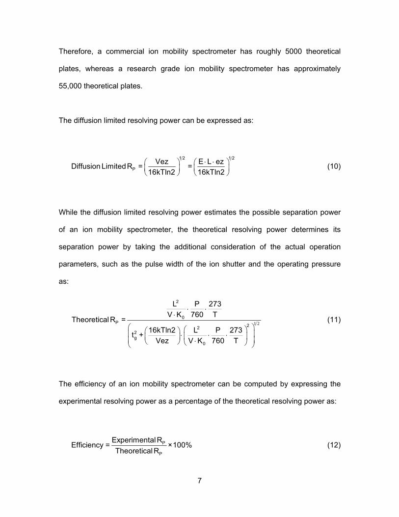
Therefore, a commercial ion mobility spectrometer has roughly 5000 theoretical

plates, whereas a research grade ion mobility spectrometer has approximately

55,000 theoretical plates.

The diffusion limited resolving power can be expressed as:

1 2 1 2

PVez E L ezDiffusion Limited R = =

16kTln2 16kTln2⋅ ⋅⎛ ⎞ ⎛ ⎞

⎜ ⎟ ⎜ ⎟⎝ ⎠ ⎝ ⎠

(10)

While the diffusion limited resolving power estimates the possible separation power

of an ion mobility spectrometer, the theoretical resolving power determines its

separation power by taking the additional consideration of the actual operation

parameters, such as the pulse width of the ion shutter and the operating pressure

as:

1 2

2

0P 22

2g

0

L P 273V K 760 T

Theoretical R =16kTln2 L P 273t +

Vez V K 760 T

⋅ ⋅⋅

⎛ ⎞⎛ ⎞⎛ ⎞⎜ ⎟⋅ ⋅ ⋅⎜ ⎟⎜ ⎟⎜ ⎟⋅⎝ ⎠ ⎝ ⎠⎝ ⎠

(11)

The efficiency of an ion mobility spectrometer can be computed by expressing the

experimental resolving power as a percentage of the theoretical resolving power as:

P

P

Experimental REfficiency = ×100%

Theoretical R (12)

8

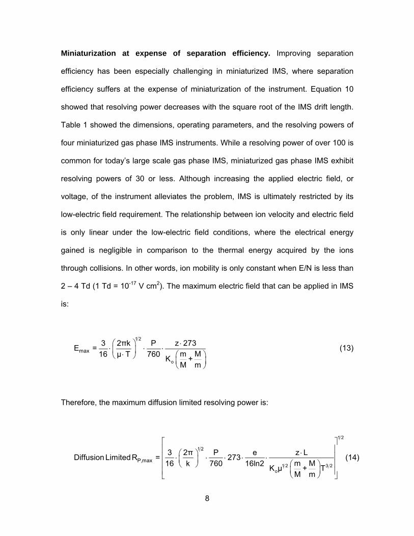
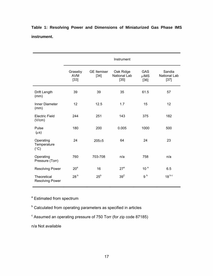
Miniaturization at expense of separation efficiency. Improving separation

efficiency has been especially challenging in miniaturized IMS, where separation

efficiency suffers at the expense of miniaturization of the instrument. Equation 10

showed that resolving power decreases with the square root of the IMS drift length.

Table 1 showed the dimensions, operating parameters, and the resolving powers of

four miniaturized gas phase IMS instruments. While a resolving power of over 100 is

common for today’s large scale gas phase IMS, miniaturized gas phase IMS exhibit

resolving powers of 30 or less. Although increasing the applied electric field, or

voltage, of the instrument alleviates the problem, IMS is ultimately restricted by its

low-electric field requirement. The relationship between ion velocity and electric field

is only linear under the low-electric field conditions, where the electrical energy

gained is negligible in comparison to the thermal energy acquired by the ions

through collisions. In other words, ion mobility is only constant when E/N is less than

2 – 4 Td (1 Td = 10-17 V cm2). The maximum electric field that can be applied in IMS

is:

1 2

o

max3 2πk P z 273E =

m M16 μ T 760 K +M m

⎛ ⎞ ⋅⋅ ⋅ ⋅⎜ ⎟⋅ ⎛ ⎞⎝ ⎠

⎜ ⎟⎝ ⎠

(13)

Therefore, the maximum diffusion limited resolving power is:

1 2

1 2

1 2 3 2o

P,max3 2π P e z LDiffusion Limited R = 273

m M16 k 760 16ln2 K μ + TM m

⎡ ⎤⎢ ⎥⋅⎛ ⎞⎢ ⎥⋅ ⋅ ⋅ ⋅ ⋅⎜ ⎟ ⎛ ⎞⎢ ⎥⎝ ⎠

⎜ ⎟⎢ ⎥⎝ ⎠⎣ ⎦

(14)

9

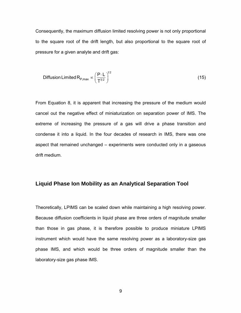
Consequently, the maximum diffusion limited resolving power is not only proportional

to the square root of the drift length, but also proportional to the square root of

pressure for a given analyte and drift gas:

1 2

3 2P,maxP LDiffusion Limited RT⋅⎛ ⎞∝ ⎜ ⎟

⎝ ⎠ (15)

From Equation 8, it is apparent that increasing the pressure of the medium would

cancel out the negative effect of miniaturization on separation power of IMS. The

extreme of increasing the pressure of a gas will drive a phase transition and

condense it into a liquid. In the four decades of research in IMS, there was one

aspect that remained unchanged – experiments were conducted only in a gaseous

drift medium.

Liquid Phase Ion Mobility as an Analytical Separation Tool

Theoretically, LPIMS can be scaled down while maintaining a high resolving power.

Because diffusion coefficients in liquid phase are three orders of magnitude smaller

than those in gas phase, it is therefore possible to produce miniature LPIMS

instrument which would have the same resolving power as a laboratory-size gas

phase IMS, and which would be three orders of magnitude smaller than the

laboratory-size gas phase IMS.

10

Nitrate ion will be used here to predict the resolving power and analysis time of a

miniaturized LPIMS in comparison with a laboratory-size gas phase IMS. Nitrate ion

has a gas phase ion mobility of 2.31 cm2 V-1 s-1 [30]. It has a drift time of 9.1 ms in a

13-cm long gas phase IMS drift tube operating at an drift voltage of 3860 V, 700 Torr

and 250 °C [30]. The diffusion-limited resolving power of this gas phase IMS system

is 88. The ion mobility of nitrate ion in water is 7.40 x 10-4 cm2 V-1 s-1 [31]. Supposed

the LPIMS instrument was reduced by a factor of 100 to 1.3 mm, which is on the

scale of a chip channel, the nitrate ion would have a drift time of 5.9 ms with the

LPIMS drift tube operating at the same drift voltage of 3860 V and at ambient

temperature. This LPIMS instrument would have a diffusion-limited resolving power

of 116, a better resolving power than the gas phase IMS instrument due to the

reduced operating temperature. The high operating temperature was required in gas

phase IMS to desolvate solvent molecules from the electrosprayed droplet. The

desolvation mechanism in LPIMS would not require high temperature and thus it

could be operated at ambient temperature.

The above nitrate calculation demonstrated that scaling down the LPIMS instrument

by two orders of magnitude, the LPIMS analysis time remained on the same

millisecond scale and LPIMS could realize a better resolving power than gas phase

IMS.

Significance of a Miniaturized High-Resolution LPIMS. The development of

LPIMS would have broad impact in the separation sciences, providing rapid

separations with high resolution. It would be suitable for military application in

11

detecting chemical and biological warfare agents, for environmental application in

detecting water contaminants, for forensic application in detecting illicit drugs and for

clinical application in detecting serum proteins. At this small scale, LPIMS could be

developed into real-time high-resolution micro sensors. The small scale also means

that LPIMS could be mass-produced in a cost-effective way and become an

inexpensive and disposable instrument.

12

Specific Aims

The primary goal of this project was to develop a miniaturized ion mobility

spectrometer in the liquid phase. While ion mobility in gases has been developed

into a successful analytical separation tool – gas phase ion mobility spectrometry,

ion mobility in liquids has never been explored as a separation technique. The

specific aims of this research are to:

1. Develop and evaluate a liquid phase ionization source suitable for LPIMS.

2. Design and construct a miniaturized separation device based on LPIMS.

3. Demonstrate the capability of LPIMS as a novel analytical detection method.

13

Attribution

The LPIMS instruments in Chapter 2, 3, and 5 were built by Tam, assisted by

Technical Service, Washington State University. The low temperature co-fired

ceramic LPIMS instrument in Chapter 4 was designed jointly by Tam, Donald

Plumlee, and Brian Jacques (from Dr. Amy Moll’s group, Materials Science and

Engineering, Boise State University), and fabricated by Plumlee and Jacques. The

poly(dimethylsiloxane) LPIMS microchannels in Chapter 4 were designed jointly by

Tam and Nazmul Al-Mamun (from Dr. Prashanta Dutta’s group, School of

Mechanical and Materials Engineering, Washington State University), and fabricated

by Al-Mamun. All the experiments were planned and conducted by Tam, except part

of the poly(dimethylsiloxane)-LPIMS experiments in Chapter 4, which was performed

by Tam and Al-Mamun. Chapter 2 and 3 were written in the format as required by

Analytical Chemistry. Chapter 5 was written in the format as required by Journal of

Chromatography. Chapter 4 was written in the format as required by the Review of

Scientific Instruments. The LabView-based data acquisition program and IGOR data

input macros were written by Brian H. Clowers [32]. Appendix III was prepared in the

format required by Analytical Chemistry (M. Tam, H. H. Hill, Jr., Analytical Chemistry,

2004, 76, 2741). The experiments and thesis were conducted under the supervision

and scientific guidance of Dr. Herbert H. Hill, Jr.

14

References

1. C. Bialobrzeski, Le Radium 8, p. 1 (1911).

2. G. Jaffé, Die elektrische Leitfähigkeit des reinen Hexans, Annalen der Physik 333, pp. 326-370 (1909).

3. I. Adamczewski, Mobilités des Ions dans la Série des carbures d'Hydrogčne Liquides et Leur Rapport avec le Coefficient de Viscositč, Annls de Physique 8, pp. 309-359 (1937).

4. R. L. Williams, Ionic Mobilities in Argon and Helium Liquids, Canadian Journal of Physics 35, p. 134 (1957).

5. L. Meyer and F. Reif, Mobilities of He Ions in Liquid Helium, Physical Review 110, pp. 279-280 (1958).

6. G. Careri, F. Scaramuzzi and J. O. Thomson, Heat Flush and Mobility of Electric Charges in Liquid Helium I. - Non Turbulent Flow, Nuovo Cimento 13, pp. 186-196 (1959).

7. K. R. Atkins, Ions in Liquid Helium, Physical Review 116, pp. 1339-1343 (1959).

8. O. Gzowski, Mobility of Ions in Liquid Dielectrics, Nature 194, p. 173 (1962).

9. I. Adamczewski and J. H. Calderwood, Viscosity and Charge Carrier Mobility in the Saturated Hydrocarbons, Journal of Physics D: Applied Physics 8, pp. 1211-1218 (1975).

10. I. Adamczewski and J. H. Calderwood, The Mobility of Fast Charge Carriers in Liquid Paraffins and its Dependence on Molecular Structure, Journal of Physics D: Applied Physics 9, pp. 2479-2483 (1976).

11. J. A. Kok, Electrical Breakdown of Insulating Liquids. Interscience Publishers, New York (1961).

12. M. J. Morant, Photo-Injection of Charge into Dielectric Liquids, Nature (London) 187, pp. 48-49 (1960).

13. A. M. Sletten, Electric Strength and High-Field Conduction Current in n-Hexane, Nature (London) 183, pp. 311-312 (1959).

14. G. Jaffé, Zur Theorie der Ionisation in Kolonnen, Annalen der Physik 347, pp. 303-344 (1913).

15

15. J. F. Fowler and F. T. Farmer, Conductivity induced in Unplasticized 'Perspex' by X-rays, Nature (London) 175, pp. 516-517 (1955).

16. H. J. Plumley, Conduction of Electricity by Dielectric Liquids at High Field Strengths, Physical Review 59, pp. 200-207 (1941).

17. I. Adamczewski, Liquid-filled Ionization Chambers as Dosimeters, Colloques Internationaux du Centre National de la Recherche Scientifique 179, pp. 21-44 (1970).

18. A. O. Allen, M. P. Haas and A. Hummel, Measurement of Ionic Mobilities in Dielectric Liquids by Means of Concentric Cylindrical Electrodes, Journal of Chemical Physics 64, pp. 2587-2592 (1976).

19. N. Houser and R. C. Jarnagin, Electron Ejection from Triplet State in Fluid Solutions, Journal of Chemical Physics 52, pp. 1069-1078 (1970).

20. S. K. Lim, M. E. Burba and A. C. Albrecht, Mobilities of Radical Cations and Anions, Dimer Radical Anions, and Relative Electron Affinities by Times of Flight in n-hexane, Journal of Physical Chemistry 98, pp. 9665-9675 (1994).

21. K. S. Haber and A. C. Albrecht, Time-of-Flight Technique for Mobility Measurements in the Condensed Phase, Journal of Physical Chemistry 88, pp. 6025-6030 (1984).

22. M. E. Burba, S. K. Lim and A. C. Albrecht, Relative Electron Affinity of C60 and C70 and the Stokes' Law Radius of the C70 Radical Anion in n-Hexane by Time-of-Flight Mobility Measurements, Journal of Physical Chemistry 99, pp. 11839-11843 (1995).

23. W. C. Röentgen, Science 3, pp. 726-729 (1896).

24. J. J. Thomson and G. P. Rutherford, Conduction of Electricity through Gases. Dover, New York (1928).

25. P. Langevin, L'Ionistiondes Gaz, Ann. de Chim. Phys. 28, pp. 289-384 (1903).

26. P. Langevin, Une Formule Fondamentale de Théorie Cinétique, Ann. de Chim. et de Phys. 5, pp. 245-188 (1905).

27. G. A. Eiceman, Advances in Ion Mobility Spectrometry - 1980-1990, Critical Reviews in Analytical Chemistry 22, pp. 17-36 (1991).

28. H. E. Revercomb and E. A. Mason, Theory of Plasma Chromatography/Gaseous Electrophoresis -- A Review, Analytical Chemistry 47, pp. 970-983 (1975).

29. R. Wilson and A. Brittain, Explosives in the Service of Man. Royal Society of Chemistry, Cambridge (1997).

16

30. G. R. Asbury and Jr. H. H. Hill, Negative Ion Electrospray Ionization Ion Mobility Spectrometry, International Journal for Ion Mobility Spectrometry 2, pp. 1-8 (1999).

31. P. W. Atkins, Physical Chemistry (5th Edn). W. H. Freeman and Company, USA (1994).

32. B. H. Clowers, Separation of Gas Phase Isomers Using Ion Mobility and Mass Spectrometry, Washington State University, Pullman WA (2005).

33. J. I. Baumbach, S. Sielemann and P. Pilzecker, Coupling of Multi-Capillary Columns with two Different Types of Ion Mobility Spectrometer, International Journal for Ion Mobility Spectrometry 3, pp. 28-37 (2000).

34. A. B. Kanu, P. E. Haigh and Jr. H. H. Hill, Surface Detection of Chemical Warfare Agent Simulants and Degradation Products, Analytica Chimica Acta 553, pp. 148-159 (2005).

35. J. Xu, W. B. Whitten and J. M. Ramsey, Space Charge Effects on Resolution in a Miniature Ion Mobility Spectrometer, Analytical Chemistry 72, pp. 5787-5791 (2000).

36. St. Sielemann, J. I. Baumbach, H. Schmidt and P. Pilzecker, Quantitative Analysis of Benzene, Toluene, and m-Xylene with the Use of a UV-Ion Mobility Spectrometer, Field Analytical Chemistry and Technology 4, pp. 157-169 (2000).

37. K. B. Pfeifer and A. N. Rumpf, Measurement of Ion Swarm Distribution Functions in Miniature Low-Temperature Co-Fired Ceramic Ion Mobility Spectrometer Drift Tubes, Analytical Chemistry 77, pp. 5215-5220 (2005).

17

Table 1: Resolving Power and Dimensions of Miniaturized Gas Phase IMS

instrument.

Instrument

Graseby

AVM [33]

GE Itemiser

[34]

Oak Ridge

National Lab [35]

GAS μIMS [36]

Sandia

National Lab [37]

Drift Length (mm)

39

39

35

61.5

57

Inner Diameter (mm)

12

12.5

1.7

15

12

Electric Field (V/cm)

244

251

143

375

182

Pulse (μs)

180

200

0.005

1000

500

Operating Temperature (°C)

24

205±5

64

24

23

Operating Pressure (Torr)

760

703-708

n/a

758

n/a

Resolving Power

20a

16

27a

10 a

6.5

Theoretical Resolving Power

28 b

25b

39C

9 b

18 b c

a Estimated from spectrum

b Calculated from operating parameters as specified in articles

c Assumed an operating pressure of 750 Torr (for zip code 87185)

n/a Not available

18

Chapter Two

Electrodispersion Ionization in Liquids

Abstract

A new ionization source, called electrodispersion ionization (EDI), was developed for

generating liquid-phase ions. EDI, the liquid-phase analogue of gas-phase

electrospray ionization (ESI), produced ions from aqueous samples in a non-

electrolyte containing liquid medium. Visualization of the electrodispersed droplets

was demonstrated with aqueous solutions of two dyes, basic fuchsin and

bromothymol blue. Continuous and stable current from electrodispersion ionization

was measured for inorganic and organic ions by a Faraday plate at a distance of 10

mm away from the ionization source. Quantitative ionization of the method was

investigated for several amino acids with detection limits measured in the low ppm

range. Under certain operation conditions, combinations of applied voltage and

sample flow rate can lead to pulsing of the ion current for the EDI source. Control of

this pulsing phenomenon may lead to the elimination of the need for an ion gate in

such applications as liquid phase ion mobility spectrometry.

19

Introduction

Mass spectrometry (MS), ion mobility spectrometry (IMS), and field asymmetric

waveform ion mobility spectrometry (FAIMS) are important analytical separation

techniques sharing a common operational feature – they all require the production of

analyte ions. The conversion of the analyte of interest into charged particles allows

distinctive ion manipulation, separation, and detection. Because analysis would be

impossible should the sample remain neutral, production of ions is a requisite for

these analytical methods. In these instruments, an ion can be accelerated and

decelerated by the use of electric and/or magnetic fields. A mixture of analyte ions

can be separated based on their mass, momentum, charge, size, and interactions

with the medium. Any ionizable chemical is capable of being detected as discharge

current by Faraday plate, or indirectly as secondary or cascading particles by

electron multiplier, photon multiplier, and multichannel plate. Furthermore, the

charge count is related to the sample concentration and thus, quantification can be

routinely accomplished. In addition, because the ions can be guided from one

spectrometer to another, the tandem coupling of these methods provides a powerful

separation process that can produce a wealth of multidimensional information.

Examples of multidimensional ion separation methods include tandem MS [1-5],

tandem IMS [6;7], tandem IMS and MS [6;8-11], tandem FAIMS and MS [12;13],

tandem FAIMS, IMS, and MS [14].

Because all of these powerful analytical methods separate charged analyte, a wide

variety of ionization methods have been developed. Electron impact ionization,

20

chemical ionization, fast atom/ion bombardment, electrospray ionization, matrix

assisted laser desorption ionization, and desorption electrospray ionization are a few

examples of established ionization methods which have been used in combination

with MS or IMS [15-25]. Although these ionization sources ionize gas, liquid, and

solid samples, they produce only gas-phase ions.

The production of liquid-phase ions have been less investigated. Radioactive

ionization, x-ray irradiation, photo-ionization, and field emission are liquid-phase

ionization sources that have been used in the studies of electrical properties of

dielectric liquids. These sources produce liquid-phase ions of liquid hydrocarbons,

insulating oils, liquefied noble gases, and the impurities within. Ionization by radiation

generated positive and negative ions of the irradiated dielectric liquids with alpha

particles emitted from radioactive substances such as polonium-210 [26-29],

bismuth-212 (ThC) and polonium-212 (ThC’) [30], and plutonium-239 [31]; gamma

particles emitted from bismuth-214 (RaC) [32]; or with a beam of x-ray [33-36]. In

photo-ionization, ions were produced by illuminating the photocathode inside the

liquid medium with an intense ultraviolet light [37;38]. Field emission in the liquid-

phase, where ions were created by applying a high voltage to a thin tungsten wire

[39-41], was basically an extension of the gas-phase field ionization techniques

devised by Müller [42].

These liquid-phase ionization methods primarily focused on ionizing the liquid

medium and thus were incompatible for the analytical purpose of selectively ionizing

a sample analyte, and not the liquid medium. Such an ionization source would be

advantageous especially for liquid phase ion mobility spectrometry (LPIMS), which is

21

being developed as a new analytical separation method [43-45]. In liquid phase ion

mobility spectrometry, aqueous analytes are ionized in a non-electrolyte containing

liquid and moved along the spectrometer by an electric field established, not by

electrolytes, but by a series of metal electrodes held at decreasing potentials.

Analytes separate based on the difference in mobilities through an electric field in a

non-electrolytic liquid medium. Imperative to the progress of LPIMS is the

development of an adequate ionization method that is capable of ionizing aqueous

solution of analytes in a non- electrolytic liquid environment.

In this paper, a new ionization source, called electrodispersion ionization (EDI), for

liquid phase is introduced. Advantages of EDI over existing liquid-phase ionization

techniques include the following: (1) EDI ionizes aqueous phase analytes; (2) EDI

ionizes the aqueous sample in a non-electrolyte containing liquid phase, eliminating

the need to create a window for external irradiation; and (3) EDI is non-radioactive.

There are two proposed EDI mechanisms: one mechanism that involves the balance

between surface tension and Coulombic repulsion, much like the charge residue

model of ESI [23]; and another mechanism that involves the ejection of charges from

the dispersed droplet, much like the ion evaporation method of ESI [23]. More

comprehensive study and theoretical assessment are required to elucidate the

mechanistic properties of the EDI process. The primary purpose of this study,

however, was to introduce this novel approach for ion production in non-electrolyte

containing liquids and to demonstrate that the ions could be produced and that they

could be transferred through a non-electrolyte containing medium and with detection

as discharge current by a Faraday plate.

22

Experimental Section

Instrumentation. First Ionization Chamber. A transparent enclosed ionization

chamber was constructed from a Pyrex culture tube (13 mm o.d., 100 mm length)

(Figure 1), including an EDI source and a Faraday plate. Aqueous sample was

injected by a Harvard syringe pump “11” (Harvard Apparatus, Holliston, MA) through

two lengths of fused silica capillary that were joined together by a metal union (250

μm bore). Voltage was applied to the metal union. The capillary entered into the

Pyrex culture tube via a polytetrafluoroethylene (PTFE)/silicone septum. A stainless

steel Faraday plate was inserted through a slit on the culture tube, cut with a rotating

blade, and sealed with silicone rubber (Technical Services, Washington State

University, Pullman, WA). Total ion current was detected by the Faraday plate,

collected and amplified (106 gain) by a Keithley 427 current amplifier (Keithley

Instruments, Cleveland, OH) and then processed by a LabView (National

Instruments, Austin, TX)-based data acquisition system written in-house [46].

Experiments Conducted in the First Ionization Chamber. The first experiment was to

electrodisperse an aqueous solution of 0.16 mM bromothymol blue into decanol.

Video of the electrodispersion process was captured with a digital camcorder at 24

frames per second and the EDI current was measured concurrently. The

bromothymol blue solution was allowed to flow in the sample capillary. When a blue

colored drop could be seen at the tip of the capillary, the sample flow was stopped.

The digital filming and current detection began. No voltage was applied to the

23

sample capillary until after 9 s had passed, when -10 kV was applied. The voltage at

the sample capillary remained at -10 kV for the remaining of the experimental run.

The effect of sample flow rate on EDI was investigated in the positive and negative

modes, with decanol as the liquid medium. Aqueous solutions of 270 μM acetic acid

and 640 μM ammonium hydroxide were used as samples. +10 kV or -10 kV was

applied to the sample capillary continuously, depending on the polarity of the

experiment. The sample flow rates varied from 0.1 to 5.0 μL/min. The culture tube

was rinsed with decanol three times between each experimental run. Current was

measured continuously for 10 minutes.

Sensitivity of EDI was shown with calibration of three amino acids, arginine, lysine,

and serine. The amino acids were dissolved individually in purified water, in

concentrations from 10 μM to 1 mM. The amino acids were electrodispersed at

+3000V into a liquid medium of decanol and the sample flow rate was maintained at

1 μL/min. Once more, the culture tube was rinsed with decanol three times between

each experimental run.

Second Ionization Chamber. A second apparatus was constructed to accommodate

the EDI source, a Faraday plate, and a paper target (Figure 2). An aqueous sample

of basic fuchsin was introduced via a fused silica capillary (25 μm i.d. and 150 μm

o.d.), with a high voltage applied to the solution in the capillary. The current was

detected by the Faraday plate, located directly behind a piece of 1” x 2” high gloss

laser paper (Hewlett Packard Company, Palo Alto, CA). Both the Faraday plate and

the paper target were virtually grounded through the current amplifier. The

24

microscope slide, used to support the piece of paper and the Faraday plate, was

immersed into a 50-mL Pyrex beaker filled with the IMS medium. Inside the beaker,

the sample capillary was positioned 10 mm away from a paper target, and

perpendicular to the target. The detected current signal was collected and amplified

by the current amplifier, and acquired by a LabView-based data acquisition system.

Experiments Conducted in the Second Ionization Chamber. In this part of

experiment, a colored sample solution was electrodispersed towards the paper

target in a liquid medium, in order to provide simple verification that the

electrodispersed sample could travel across the liquid medium and arrive at the

detector. The experiment was first conducted in air with electrospray ionization (ESI),

and then repeated in hexane and benzene with EDI for comparison between the two

similar ionization sources. The beaker was unfilled during the ESI experiment, and

filled with hexane or benzene in the EDI experiments. 10 μM of basic fuchsin was

delivered at a rate of 0.5 μL/min. Aqueous solution of basic fuchsin had various

intensities of pink, depending on the concentration of the solution. The ionization

voltage of +2000 V was applied at 15 s after data collection started, for an interval of

100 s, and was terminated at 115 s. A photograph of each piece of paper was

immediately taken after each experiment with a digital camera. A fresh piece of

paper was used for each experiment.

Chemicals. The liquid media used in the experiments were decanol (Aldrich

Chemical, Milwaukee WI), benzene (Fisher Scientific, Fair Lawn NJ), and hexane (J.

T. Baker, Phillipsburg NJ). 0.16 mM of bromothymol blue solution was prepared in

25

methanol-water (50:50, vol/vol) with 0.3% ammonium hydroxide. This was to ensure

that bromothymol blue, with a pKa of 7.10 [47] be present dominantly in its anionic

form, where over 99.99% of bromothymol blue was present as anions in 0.3%

ammonium hydroxide. HPLC grade methanol (JT Baker, Phillipsburg NJ) and 18.1

MΩ water were used. 640 μM of ammonium hydroxide solution was diluted from

30% stock standard (JT Baker, Phillipsburg NJ) in methanol-water (50:50, vol/vol).

270 μM of acetic acid solution was diluted from 37% stock standard (Fisher

Scientific, Fair Lawn NJ) in methanol-water (50:50, vol/vol). L-Lysine, L-Arginine, and

L-Serine (Sigma Chemical, St. Louis MO) were dissolved individually in water as 100

mM solutions. Additional solutions ranging in concentrations from 10 μM to 10 mM

were prepared by diluting from these 100 mM stock solutions. The aqueous solution

of 10 μM basic fuchsin, 4-((4-amino-3-methylphenyl)(4-aminophenyl)methylene)

cyclohexa-2,5-dieniminium chloride, was prepared in methanol-water (90:10,

vol/vol).

Calculations. The pH values and speciation of arginine, lysine and serine solutions

in Table 1 were calculated by solving the acid dissociation equilibriums, charge

balance, and mass balance [48].

For determining the ionization efficiency of electrodispersion ionization, the

experimental current (IExperimental) data was compared with the theoretical current.

Theoretical current (ITheoretical) is the amount of current obtained from all of the

samples introduced, by considering the sample concentration (c) and the sample

flow rate (f):

26

TheoreticalI = c × f ×F (1)

where F is Faraday’s constant. The ionization efficiency was defined by expressing

the experimental current as a percentage of the theoretical current:

Experimental

Theoretical

IIonization Efficiency = × 100%

I (2)

Results and Discussions

Digital Imaging of Electrodispersion Ionization. This experiment was conducted

in the apparatus depicted in Figure 1, with decanol as the liquid medium. The

photographs in Figure 3 were captured as still frames from the digital film of the

electrodispersion process. The time, at which the frames were captured, was labeled

underneath each photograph. A drop of bromothymol blue solution was suspended

at the end of the capillary, as shown in Figure 3A. There was no sample flow. An EDI

voltage of -10 kV was applied from 9.5 s until the end of the run. From the

procession of images, the blue drop of bromothymol blue was observed to gradually

reduce in size over time, until it was no longer visible. In addition, there was mist of

tiny droplets streaming from the end of the sample capillary. The mist was marked

with dotted circles on the photographs where it was more noticeable, in Figures 3C-

G, and 3P.

27

The corresponding current signal, measured at the Faraday plate, was plotted

against time in Figure 4. There was no current from 0 s to 9 s, when no voltage had

been applied to the sample capillary. The related photographs in Figure 3A and 3B,

at 0 s and 5 s, showed that the bromothymol blue droplet remained stationary at the

end of the capillary. After the -10 kV was applied from 9.5 s, the current rose to 0.7

μA (Figure 3). The bromothymol blue droplet in Figure 3C, at 10 s, was observed to

burst away from the capillary and a small mist of droplets was noticed around the

end of the capillary. The current gradually decreased from 0.7 μA to 0.48 μA over the

next twenty seconds (Figure 4). Figures 3D-P showed the bromothymol blue droplet

gradually reduced in size. The bromothymol blue droplet was last visible in Figure 3K

at 18 s and the final mist of droplets was visible in Figure 3P at 26 s. The current

experienced a sharp decay at 25.4 s, from 0.48 μA to 0.00 μA. The current remained

at zero level from 30 s to 60 s (Figure 4) and there was no bromothymol blue drop or

mist of droplets observable in Figure 3Q-T. The correlation between the

photographic procession and the current signal of the electrodispersion ionization

confirmed that the current measured resulted from the electrodispersed aqueous

sample. Similar images and corresponding current data from the EDI process were

obtained using aqueous solution of 0.3% ammonium hydroxide and methanol-water

solvent (50:50, vol/vol) (not shown).

Visual Evidence of Ion Transport through a Non-electrolyte Containing Liquid

Medium. While current data of electrodispersive ionization from the previous section

proved that aqueous ions were produced in the organic medium and that the ions

had traveled a distance to reach the detector, it was uncertain whether the current

28

originated from the sample or from oxidation of the liquid medium. More direct proof

was necessary to eliminate doubts that ions did travel from the ionization source,

through the liquid medium, to the detector. The method proposed was to

electrodisperse an aqueous solution of a dye into the liquid medium, position a piece

of paper at a distance from the ionization source, and watch for a color spot to

appear on the piece of paper.

The second ionization chamber (Figure 2) was used for this experiment. EDI in

hexane and in benzene was compared with ESI in air. Aqueous sample of 10 μM

basic fuchsin was delivered continuously at 0.5 μL/min and the EDI voltage of

+2000V was applied between 15 s and 115 s. It was observed that the total ion

current of EDI in hexane and benzene was comparable to that of ESI in air (Figure

5). There was zero current when the ionization voltage was not applied. The current

rose after the voltage was switched on at 15 s and the current remained at a steady

level until the voltage was switched off at 115 s, after which the current gradually

decayed back to the zero current. The time taken for the current to decay to zero

after the voltage had terminated was 3.2 s, 6.7 s, and 8.3 s for ESI in air, EDI in

hexane, and EDI in benzene, respectively. The apparent current spike at 15 s was

due to a ringing resulting from switching on the high voltage power supply. The

current level for ESI in air was 0.34 ± 0.02 nA, 0.80 ± 0.01 nA for EDI in hexane, and

1.02 ± 0.02 nA for EDI in benzene.

Photographs of the corresponding pieces of paper showed pink spots of basic

fuchsin from electrospray in air, electrodispersion in hexane and benzene (Figure 6).

29

The diameter of the pink dye was the widest for ESI in air (1.03 mm), followed by

that of EDI in hexane (0.52 mm), and of EDI in benzene (0.29 mm). Coulombic

repulsion of the ionization spray is much larger in air than in the liquid due to the

three orders of magnitude difference in diffusion between the gas phase and the

liquid phase. The initial ion plume was speculated to be broader in air than in liquids,

and thus resulting in a wider spot on the paper target in air. The difference in size of

the pink dye between the two liquid media could be associated with their difference

in viscosity. The viscosity of hexane was 0.326 cP and that of benzene was 0.604 cP

[49]. The mobility and diffusion of an ion is inversely proportional to the viscosity of

the medium [50-52]. Hence, the diffusion of ions is faster in hexane than in benzene,

and this resulted in a wider spot on the paper target in hexane.

Effect of Sample Flow Rates. The effect of sample flow rates was investigated in

the apparatus depicted in Figure 1. The current detected on the Faraday plate was

plotted versus time for the two samples, 270 μM acetic acid (Figure 7a) and 640 μM

ammonium hydroxide (Figure 7b) for the range of sample flow rates. A steady ion

current was measured for flow rates from 1.5 to 5.0 μL/min, and the current

increased with the flow rates from 0.208 to 0.292 μA for acetic acid and from 0.180

to 0.314 μA for ammonium hydroxide, with an average noise of 0.002 μA. However,

at sample flow rates of 1.0 μL/min and below, the ion current was periodic. As the

sample flow rate decreased, the period between current lengthened and the current

period shortened. For the positive mode, the period decreased from 29 s, 23 s, to 15

s, for 1.0, 0.5, and 0.1 μL/min of sample flow rate, respectively. For the negative

30

mode, the interval increased from 7 s, 25 s, to 99 s, for 1.0, 0.5, and 0.1 μL/min of

sample flow rate, respectively.

As the flow rate was reduced, with the EDI voltage maintained at 10 kV, the sample

ions were in fact ejected at a faster rate than they were being delivered.

Consequently, there existed a period of time when the sample was depleted of

analytes and no current was measured. When the flow rate increased, the sample

depletion rate decreased, and the period of zero-current was abbreviated. When the

flow rate was sufficiently fast, at 1.5 μL/min and above, analytes were no longer

completely depleted from the sample and a continuously stable current was

observed. Alternatively, a stable ion current could be achieved at the lower flow rates

with a lower EDI voltage, demonstrating that the EDI source could operate in a

continuous or pulsed mode, by adjusting the applied voltage in relation to the sample

flow rate. The advantage of having a pulsed ionization source is the possible

omission of a physical ion shutter, and thus simplifying the process of miniaturizing

an ion mobility spectrometer. Moreover, smaller sample volumes would be required

for pulsed ionization, as the sample would not be continuously ionized and

dispersed.

Calibration of Amino Acids. Figure 8 demonstrates the quantitative response of

three amino acids: arginine, lysine, and serine, using the first ionization chamber.

The amino acids were dissolved in water, with no additional organic solvents or

acids. Concentrations from 10 μM to 1 mM were used, with a sample flow rate of 1

μL/min and an EDI voltage of +3000V. It was observed that the current increased

31

with concentration for lysine and arginine, yet the current did not change appreciably

with concentration for serine (Figure 8). The calibration slope for arginine was 1.68

mA/ mM and 1.39 mA/ mM for lysine. The detection limit, as defined as three times

the noise level, was 31 μM (5.4 ppm) for arginine and 12 μM for lysine (1.8 ppm).

The difference in sensitivities among lysine, arginine, and serine may have been

related to their pKa values. Table 1 provides the speciation of these amino acids in

the unbuffered solution as a function of concentration and pH. Under the conditions

used in this experiment, serine existed primarily as the neutral species and thus did

not ionize appreciably during the electrodispersion process. On the other hand,

lysine with a pKa of 10.3 [53] and arginine with a pKa of 13.2 [53] existed

predominantly in the 1+ state (MH+).

For concentrations between 10 μM and 1 mM of arginine and lysine, more than

99.5% were present as the singly charged (MH)+, fewer than 0.02% as the doubly

charged (M+2H)2+, fewer than 0.5% as the neutral species, and a negligible amount

as the negatively charged (M-H)- (Table 1). In contrast, fewer than 0.02% of serine

are present as (MH)+, more than 99.5% are neutral, and fewer than 0.5% are

negatively charged (Table 1). The results showed that when the sample analyte was

largely present as its neutral species, there was an insignificant amount of current

signal detected. However, when the sample analyte was present mostly in its ionized

form, there was ample detectable current. These results suggested electrodispersion

ionization was a process capable of transferring ions pre-existing in the aqueous

sample solution and dispersing them into the organic liquid medium.

32

Efficiency of Ionization. The ionization efficiency of electrodispersion ionization,

interpreted as a percentage of the theoretical ion output, was determined for the

above EDI experiments of basic fuchsin, ammonium hydroxide, acetic acid, arginine,

and lysine (Table 2). Data for 10 μM of arginine and lysine were not included as this

concentration was below the detection limit for both amino acids. For basic fuchsin,

ammonium hydroxide, and acetic acid, the average ionization efficiency was 15%.

The average ionization efficiency for arginine and lysine was 86%. It was not

apparent on why there were more ions detected than ions injected at 50 and 100 μM

of arginine and lysine, although this may have been due to the existence of doubly

charged species under these conditions. The EDI data of the ammonium hydroxide

and acetic acid showed that the ionization efficiency increased with decreasing

sample flow rate, which was also observed with ESI in gas phase IMS [54].

Conclusions

The results demonstrate the viability of a new ionization method suitable for the

ionization of analytes from aqueous phase samples in non-electrolyte containing

liquids. This ionization method may be especially useful in combination with liquid

phase ion mobility spectrometry and other liquid phase separation methods for ions.

Electrodispersion ionization is effective in delivering pre-existent positive and

negative ions from aqueous sample solution and dispersing them into the organic

liquid medium, with its ionization efficiency dependent upon the sample flow rate.

Electrodispersion ionization is capable of ionizing aqueous solutions of inorganic and

organic analytes in non-aqueous liquid medium. Furthermore, electrodispersion

33

ionization can operate in continuous and pulsing modes. In addition to its potential

use as an ionization method for analytical methods, it may be useful for the creation

of ions or the dispersion of reactants into non-aqueous phases for chemical

syntheses.

Acknowledgements

This work was supported by the National Institutes of Biomedical Imaging and

Bioengineering, National Institutes of Health (Grant R21EB001950).

34

References

1. A. K. Shukla and J. H. Futrell, Tandem Mass Spectrometry: Dissociation of Ions by Collisional Activation, Journal of Mass Spectrometry 35, pp. 1069-1090 (2000).

2. K. F. Medzihradszky, J. M. Campbell, M. A. Baldwin, A. M. Falick, P. Juhasz, M. L. Vestal and A. L. Burlingame, The Characteristics of Peptide Collision-Induced Dissociation Using a High-Performance MALDI-TOF/TOF Tandem Mass Spectrometer, Analytical Chemistry 72, pp. 552-558 (2000).

3. J. N. Louris, J. S. Brodbeltlustig, R. G. Cooks, G. L. Glish, G. J. Vanberkel and S. A. McLuckey, Ion Isolation and Sequential Stages of Mass-Spectrometry in a Quadrupole Ion Trap Mass-Spectrometer, International Journal of Mass Spectrometry and Ion Processes 96, pp. 117-137 (1990).

4. J. V. Johnson, R. A. Yost, P. E. Kelley and D. C. Bradford, Tandem-in-Space and Tandem-in-Time Mass-Spectrometry - Triple Quadrupoles and Quadrupole Ion Traps, Analytical Chemistry 62, pp. 2162-2172 (1990).

5. F. W. McLafferty, Tandem Mass Spectrometry. John Wiley, New York (1983).

6. S. I. Merenbloom , S. L. Koeniger, S. J. Valentine, M. D. Plasencia and D. E. Clemmer, IMS-IMS and IMS-IMS-IMS/MS for Separating Peptide and Protein Fragment Ions, Analytical Chemistry 78, pp. 2802-2809 (2006).

7. S. L. Koeniger, S. I. Merenbloom, S. J. Valentine, M. F. Jarrold, H. R. Udseth, R. D. Smith and D. E. Clemmer, An IMS-IMS Analogue of MS-MS, Analytical Chemistry 78 , pp. 4161-4174 (2006).

8. B. K. Bluhm, K. J. Gilig and D. H. Russell, Development of a Fourier-Transform Ion Cyclotron Resonance Mass Spectrometer-Ion Mobility Spectrometer, Review of Scientific Instruments 71, pp. 4078-4086 (2000).

9. F. W. Karasek, S. H. Kim and Jr. H. H. Hill, Mass Identified Mobility Spectra of p-Nitrophenol and Reactant Ions in Plasma Chromatography, Analytical Chemistry 48, pp. 1133-1137 (1976).

10. B. H. Clowers and Jr. H. H. Hill, Mass Analysis of Mobility-Selected Ion Populations Using Dual Gate-Ion Mobility-Quadrupole Ion Trap Mass Spectrometry, Analytical Chemistry 77, pp. 5877-5882 (2005).

11. R. Guevremont, K. W. M. Siu, J. Y. Wang and L. U. Ding, Combined Ion Mobility Time-Of-Flight Mass Spectrometry Study Of Electrospray-Generated Ions, Analytical Chemistry 69, pp. 3959-3965 (1997).

35

12. R. Guevremont and R. W. Purves, High Field Asymmetric Waveform Ion Mobility Spectrometry-Mass Spectrometry: An Investigation of Leucine Enkephalin Ions Produced by Electrospray Ionization, Journal of the American Society for Mass Spectrometry 10, pp. 492-501 (1999).

13. E. W. Robinson, D. E. Garcia, R. D. Leib and E. R. Williams, Enhanced Mixture Analysis of Poly(Ethylene Glycol) Using High-Field Asymmetric Waveform Ion Mobility Spectrometry Combined with Fourier Transform Ion Cyclotron Resonance Mass Spectrometry, Analytical Chemistry 78, pp. 2190-2198 (2006).

14. K. Q. Tang, F. M. Li, A. A. Shvartsburg, E. F. Strittmatter and R. D. Smith, Two-Dimensional Gas-Phase Separations Coupled to Mass Spectrometry for Analysis of Complex Mixtures, Analytical Chemistry 77, pp. 6381-6388 (2005).

15. M. Barber, Fast Atom Bombardment Mass Spectrometry, Analytical Chemistry 54, pp. A645-657 (1982).

16. C. B. Shumate and Jr. H. H. Hill, Coronaspray Nebulization and Ionization of Liquid Samples for Ion Mobility Spectrometry, Analytical Chemistry 61, pp. 601-606 (1989).

17. S. Lee, T. Wyttenbach and M. T. Bowers, Gas Phase Structures of Sodiated Oligosaccharides by Ion Mobility Ion Chromatography Methods, International Journal of Mass Spectrometry 167, pp. 605-614 (1997).

18. S. Myung, J. M. Wiseman, S. J. Valentine, Z. Takats, R. G. Cooks and D. E. Clemmer, Coupling Desorption Electrospray Ionization with Ion Mobility/Mass Spectrometry or Analysis of Protein Structure: Evidence for Desorption of Folded and Denatured States, Journal of Physical Chemistry B 110, pp. 5045-5051 (2006).

19. R. W. Purves and R. Guevremont, Electrospray Ionization High-Field Asymmetric Waveform Ion Mobility Spectrometry-Mass Spectrometry, Analytical Chemistry 71, pp. 2346-2357 (1999).

20. A. O. Nier, A Mass Spectrometer for Isotope and Gas Analysis, Review of Scientific Instruments 18, pp. 398-411 (1947).

21. A. G. Harrison, Chemical Ionization Mass Spectrometry. CRC Press, Boca Raton, FL (1983).

22. M. Barber, R. S. Bardoli and R. D. Segwick, Fast Atom Bombardment of Solids (F.A.B.): A New Ion Source for Mass Spectrometry, Journal of the Chemical Society, Chemical Communications pp. 325-327 (1981).

23. P. Kebarle, A Brief Overview of the Present Status of the Mechanisms Involved in Electrospray Mass Spectrometry, Journal of Mass Spectrometry 35, pp. 804-817 (2000).

36

24. Z. Takats, J. M. Wiseman, B. Gologan and R. G. Cooks, Mass Spectrometry Sampling Under Ambient Conditions with Desorption Electrospray Ionization, Science 306, pp. 471-473 (2004).

25. M. Karas, U. Bahr and U. Giessman, Matrix-Assisted Laser Desorption Ionization Mass-Spectrometry, Mass Spectrometry Reviews 10, pp. 335-357 (1991).




29. G. Aniansson, New Method for Measuring the α-Particle Range and Straggling in Liquids, Physical Review 98, pp. 300-302 (1955).

30. M. S. Malkin and H. L. Schultz, Electron Mobilities in Liquid Argon, Physical Review 83, pp. 1051-1052 (1951).

31. D. W. Swan, Electron Attachment Processes in Liquid Argon containing Oxygen or Nitrogen Impurity, Proceedings of the Physical Society (London) 82, pp. 74-84 (1963).

32. G. W. Hutchinson, Ionization in Liquid and Solid Argon, Nature 162, pp. 610-611 (1948).

33. O. Gzowski and J. Terlecki, A Method for Measuring the Mobility of Ions in Dielectric Liquids, Acta Physica Polonica 18, pp. 191-198 (1959).

34. O. Gzowski, Mobility of Ions in Liquid Dielectrics, Nature 194 , p. 173 (1962).

35. B. Jachym, Mobility of Ions in Dielectric Liquids of High Viscosity, Acta Physica Polonica 24, pp. 785-790 (1963).

36. B. Jachym, Ion Mobility in Liquid Cyclohexane, Acta Physica Polonica 24, pp. 243-247 (1963).

37. O. H. LeBlanc. Jr., Electron Drift Mobility in Liquid n-Hexane, Journal of Chemical Physics 30, pp. 1443-1447 (1959).

38. J. Terlecki, Measurement of the Mobility of Negative Ions in Saturated Hydrocarbon Liquids with High Electric Fields, Nature 194, pp. 172-173 (1962).

39. B. L. Henson, Mobility of Positive Ions in Liquefied Argon and Nitrogen, Physical Review 135, pp. A1002-1008 (1964).

37

40. B. Halpern and R. Gomer, Field Ionization in Liquids, Journal of Chemical Physics 51, pp. 1048-1056 (1969).

41. B. Halpern and R. Gomer, Field Emission in Liquids, Journal of Chemical Physics 51, pp. 1031-1047 (1969).

42. E. W. Müller and K. Bahadur, Field Ionization of Gases at a Metal Surface and the Resolution of the Field Ion Microscope, Physical Review 102, pp. 624-631 (1956).

43. H. H. Hill, Jr. and M. Tam. Ion Mobility Spectrometry Method and Apparatus. US Patent. 7,071,465. July 4, 2006.

44. M. Tam and H. H. Hill, Jr. Liquid Phase Ion Mobility Spectrometry. 14th International Symposium on Ion Mobility Spectrometry. Paris, France. 2005.

45. M. Tam and H. H. Hill, Jr. Analytical Detection by Liquid Phase Ion Mobility Spectrometry. 54th American Society for Mass Spectrometry Conference on Mass Spectrometry. Seattle, WA. 2006.


47. D. Gupta, Journal of Pharmaceutical Science 57, pp. 2140-2142 (1968).

48. M. M. Benjamin, Water Chemistry. McGraw-Hill, New York (2001).

49. D. R. Lide, CRC Handbook of Chemistry and Physics (85th Edn). CRC Press, Boca Raton, FL (2004).

50. D. R. Baker, Capillary Electrophoresis. John Wiley & Sons, Inc., New York, NY (1995).

51. J. S. Townsend, The Diffusion of Ions into Gases, Philosophical Transactions of the Royal Society of London A193, pp. 129-158 (1900).

52. W. Nernst, Zur Kinetik der in Lösung befindlichen Körper - I. Theorie der Diffusion, Zeitschrift fuer Physikalische Chemie 2, pp. 613-637 (1888).

53. S. Budavari, The Merck Index (12th Edn). Merck Research Laboratories, Whitehouse Station NJ (1996).

54. X. Tang, J. E. Bruce and Jr. H. H. Hill, Characterizing Electrospray Ionization Using Atmospheric Pressure Ion Mobility Spectrometry, Analytical Chemistry 78, pp. 7751-7760 (2006).

38

Table 1: Solution pH values and speciation information for arginine, lysine,

and serine at concentrations from 10 μM to 1 mM.

Fractional Dissociation

Amino Acid

Formal Conc. (mM)

pH

(M+2H)2+

(M+H)+

M

(M-H)-

Arginine 0.01 6.87 0.002% 99.531% 0.467% 0.000%

0.05 6.65 0.004% 99.715% 0.281% 0.000% 0.10 6.52 0.005% 99.785% 0.210% 0.000% 0.50 6.21 0.010% 99.889% 0.101% 0.000% 1.00 6.07 0.013% 99.912% 0.075% 0.000%

Lysine 0.01 6.82 0.002% 99.578% 0.419% 0.000% 0.05 6.57 0.004% 99.761% 0.234% 0.000% 0.10 6.44 0.006% 99.822% 0.172% 0.000% 0.50 6.11 0.012% 99.906% 0.082% 0.000% 1.00 5.98 0.017% 99.923% 0.060% 0.000%

Serine 0.01 6.10 n/a 0.012% 99.907% 0.080% 0.05 6.24 n/a 0.009% 99.882% 0.109%

0.10 6.55 n/a 0.004% 99.772% 0.223% 0.50 6.67 n/a 0.003% 99.700% 0.297% 1.00 6.88 n/a 0.002% 99.517% 0.481%

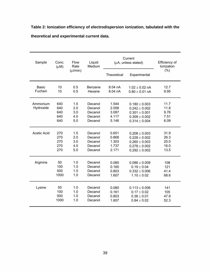
39

Table 2: Ionization efficiency of electrodispersion ionization, tabulated with the

theoretical and experimental current data.

Current

(μA, unless stated)

Sample

Conc. (μM)

Flow Rate

(μl/min)

Liquid Medium

Theoretical

Experimental

Efficiency of Ionization

(%)

10 0.5 Benzene 8.04 nA 1.02 ± 0.02 nA 12.7 Basic

Fuchsin 10 0.5 Hexane 8.04 nA 0.80 ± 0.01 nA 9.95

640 1.5 Decanol 1.544 0.180 ± 0.003 11.7 640 2.0 Decanol 2.058 0.242 ± 0.002 11.8 640 3.0 Decanol 3.087 0.301 ± 0.001 9.76 640 4.0 Decanol 4.117 0.309 ± 0.002 7.51

Ammonium Hydroxide

640 5.0 Decanol 5.146 0.314 ± 0.004 6.09

270 1.5 Decanol 0.651 0.208 ± 0.003 31.9 270 2.0 Decanol 0.868 0.228 ± 0.002 26.3 270 3.0 Decanol 1.303 0.260 ± 0.003 20.0 270 4.0 Decanol 1.737 0.278 ± 0.002 16.0

Acetic Acid

270 5.0 Decanol 2.171 0.292 ± 0.002 13.5

50 1.0 Decanol 0.080 0.086 ± 0.009 108 100 1.0 Decanol 0.160 0.19 ± 0.04 121 500 1.0 Decanol 0.803 0.332 ± 0.006 41.4

Arginine

1000 1.0 Decanol 1.607 1.10 ± 0.02 68.6

50 1.0 Decanol 0.080 0.113 ± 0.006 141 100 1.0 Decanol 0.161 0.17 ± 0.02 105 500 1.0 Decanol 0.803 0.38 ± 0.01 47.9

Lysine

1000 1.0 Decanol 1.607 0.84 ± 0.02 52.3

40

Figure Captions

Figure 1: Schematic of the electrodispersion ionization apparatus. The ionization

chamber was built using a Pyrex culture tube (A) closed with an open top screw cap

(B) and a polytetrafluoroethylene (PTFE)/silicone septum (C). The aqueous sample

was delivered through a fused silica capillary (D), which had a high voltage applied

to it via a metal connection. The current was measured at the Faraday plate (E).

Figure 2: Schematic of the second electrodispersion ionization apparatus. The

ionization apparatus included a fused silica capillary (A) for delivering aqueous

sample, a paper target (B) and a Faraday plate (C) for detection, and a microscope

slide (D) for supporting the paper target and the Faraday plate. The ionization

apparatus was housed inside a 50-mL Pyrex beaker (E) filled with the appropriate

liquid medium.

Figure 3: Timed photographs of electrodispersion ionization. A drop of bromothymol

blue solution was introduced into a liquid medium of decanol through a fused silica

capillary. The time, at which the photograph was captured, was labeled underneath

the individual photograph. There was no applied EDI voltage from 0 s to 9.5 s, after

which -10 kV was applied until 60 s.

Figure 4: Current generated from electrodispersion ionization. An aqueous solution

of Bromothymol Blue was electrodispersed into a liquid medium of decanol. The

signal corresponded to the photographs in Figure 3.

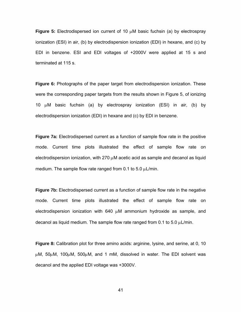
41

Figure 5: Electrodispersed ion current of 10 μM basic fuchsin (a) by electrospray

ionization (ESI) in air, (b) by electrodispersion ionization (EDI) in hexane, and (c) by

EDI in benzene. ESI and EDI voltages of +2000V were applied at 15 s and

terminated at 115 s.

Figure 6: Photographs of the paper target from electrodispersion ionization. These

were the corresponding paper targets from the results shown in Figure 5, of ionizing

10 μM basic fuchsin (a) by electrospray ionization (ESI) in air, (b) by

electrodispersion ionization (EDI) in hexane and (c) by EDI in benzene.

Figure 7a: Electrodispersed current as a function of sample flow rate in the positive

mode. Current time plots illustrated the effect of sample flow rate on

electrodispersion ionization, with 270 μM acetic acid as sample and decanol as liquid

medium. The sample flow rate ranged from 0.1 to 5.0 μL/min.

Figure 7b: Electrodispersed current as a function of sample flow rate in the negative

mode. Current time plots illustrated the effect of sample flow rate on

electrodispersion ionization with 640 μM ammonium hydroxide as sample, and

decanol as liquid medium. The sample flow rate ranged from 0.1 to 5.0 μL/min.

Figure 8: Calibration plot for three amino acids: arginine, lysine, and serine, at 0, 10

μM, 50μM, 100μM, 500μM, and 1 mM, dissolved in water. The EDI solvent was

decanol and the applied EDI voltage was +3000V.

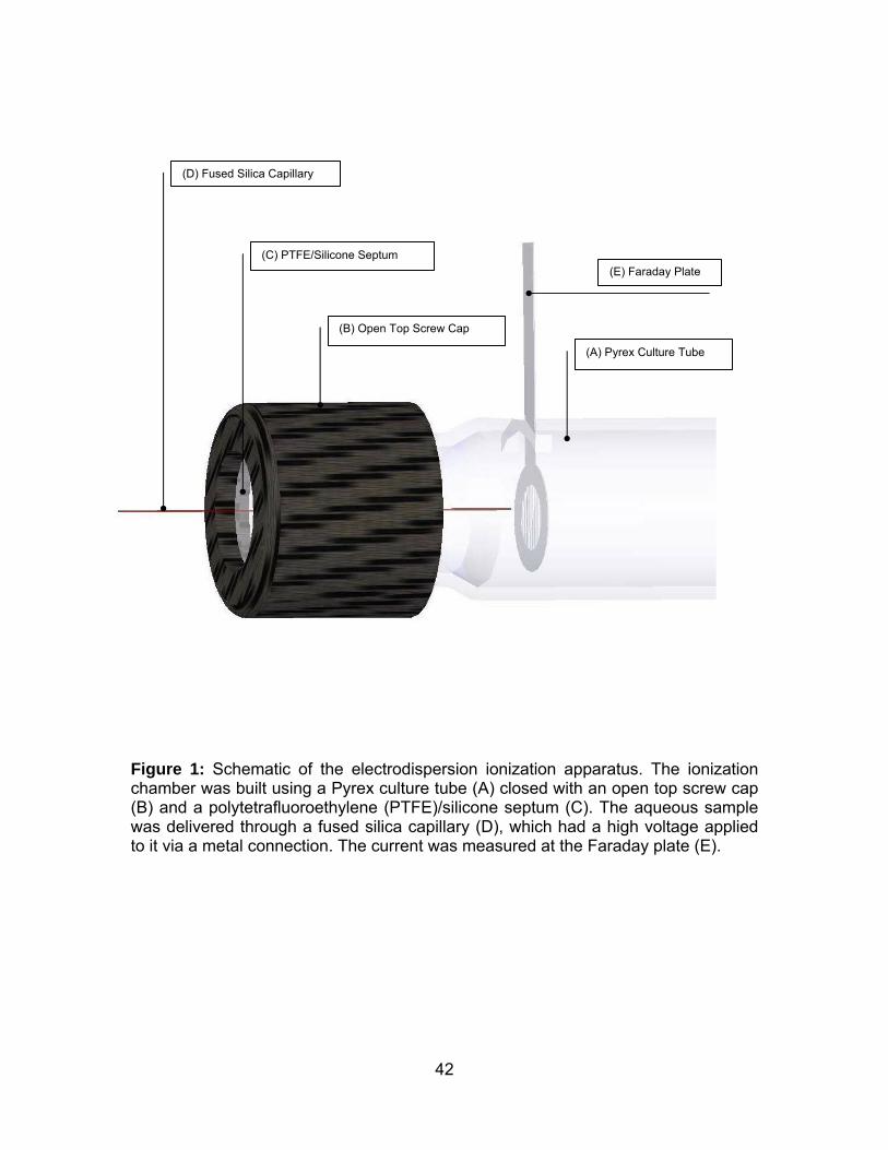
42

Figure 1: Schematic of the electrodispersion ionization apparatus. The ionization chamber was built using a Pyrex culture tube (A) closed with an open top screw cap (B) and a polytetrafluoroethylene (PTFE)/silicone septum (C). The aqueous sample was delivered through a fused silica capillary (D), which had a high voltage applied to it via a metal connection. The current was measured at the Faraday plate (E).

(D) Fused Silica Capillary

(C) PTFE/Silicone Septum

(B) Open Top Screw Cap

(E) Faraday Plate

(A) Pyrex Culture Tube

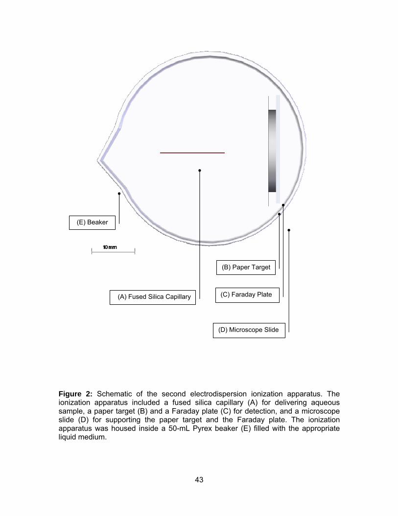
43

Figure 2: Schematic of the second electrodispersion ionization apparatus. The ionization apparatus included a fused silica capillary (A) for delivering aqueous sample, a paper target (B) and a Faraday plate (C) for detection, and a microscope slide (D) for supporting the paper target and the Faraday plate. The ionization apparatus was housed inside a 50-mL Pyrex beaker (E) filled with the appropriate liquid medium.

(C) Faraday Plate (A) Fused Silica Capillary

(B) Paper Target

(D) Microscope Slide

(E) Beaker

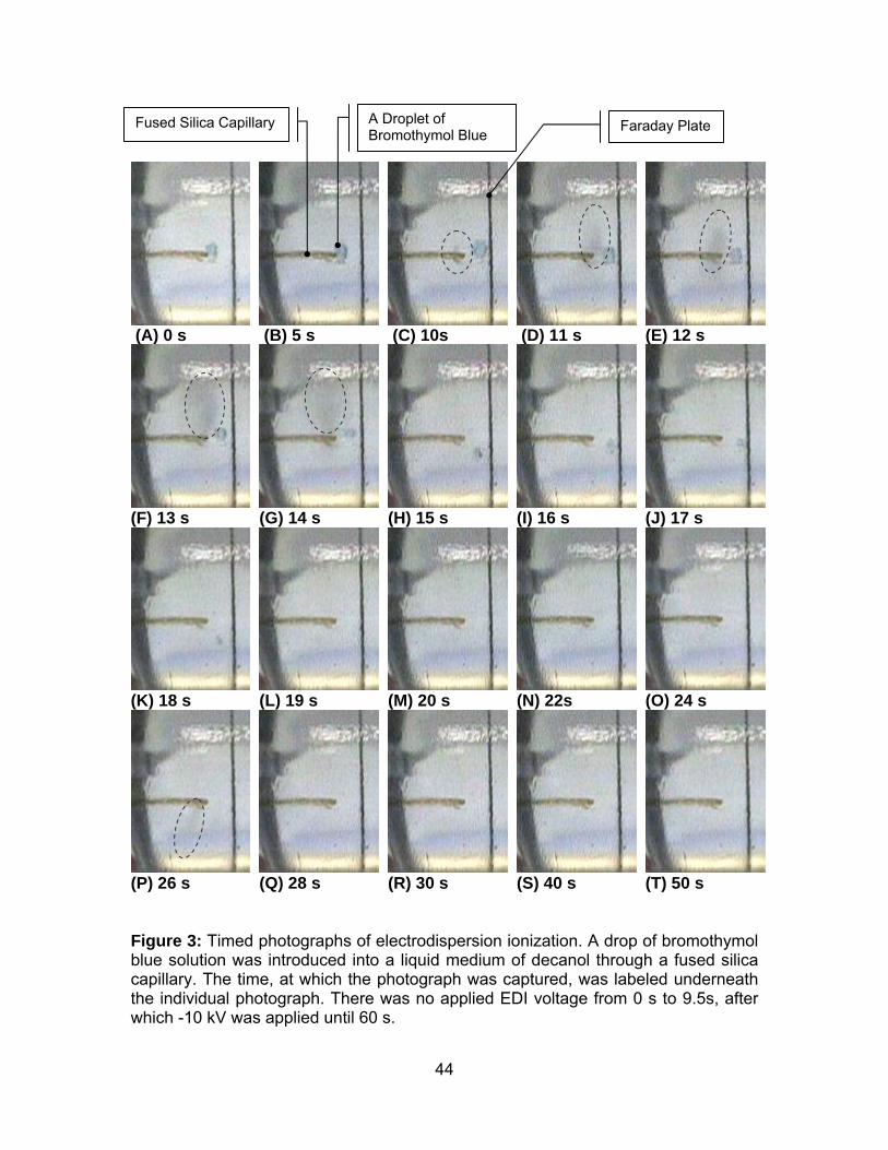
44

(A) 0 s (B) 5 s (C) 10s (D) 11 s (E) 12 s

(F) 13 s (G) 14 s (H) 15 s

(I) 16 s (J) 17 s

(K) 18 s (L) 19 s (M) 20 s

(N) 22s (O) 24 s

(P) 26 s (Q) 28 s (R) 30 s

(S) 40 s (T) 50 s

Figure 3: Timed photographs of electrodispersion ionization. A drop of bromothymol blue solution was introduced into a liquid medium of decanol through a fused silica capillary. The time, at which the photograph was captured, was labeled underneath the individual photograph. There was no applied EDI voltage from 0 s to 9.5s, after which -10 kV was applied until 60 s.

A Droplet of Bromothymol Blue

Fused Silica Capillary Faraday Plate

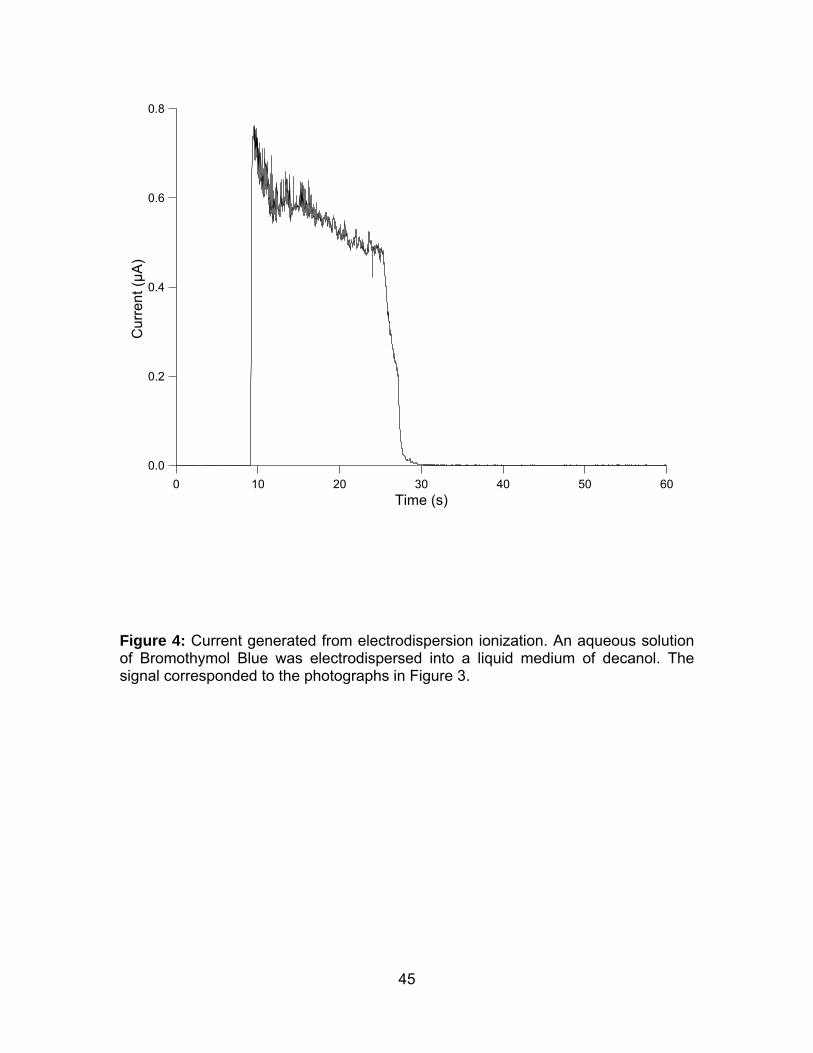
45

0.8

0.6

0.4

0.2

0.0

Cur

rent

(µA

)

6050403020100Time (s)

Figure 4: Current generated from electrodispersion ionization. An aqueous solution of Bromothymol Blue was electrodispersed into a liquid medium of decanol. The signal corresponded to the photographs in Figure 3.

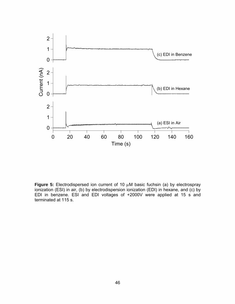
46

2

1

0

160140120100806040200Time (s)

2

1

0Cur

rent

(nA

)2

1

0

(a) ESI in Air

(b) EDI in Hexane

(c) EDI in Benzene

Figure 5: Electrodispersed ion current of 10 μM basic fuchsin (a) by electrospray ionization (ESI) in air, (b) by electrodispersion ionization (EDI) in hexane, and (c) by EDI in benzene. ESI and EDI voltages of +2000V were applied at 15 s and terminated at 115 s.

47

Figure 6: Photographs of the paper target from electrodispersion ionization. These were the corresponding paper targets from the results shown in Figure 5, of ionizing 10 μM basic fuchsin (a) by electrospray ionization (ESI) in air, (b) by electrodispersion ionization (EDI) in hexane and (c) by EDI in benzene.

(a) ESI in Air (b) EDI in Hexane (c) EDI in Benzene

1 mm 1 mm 1 mm

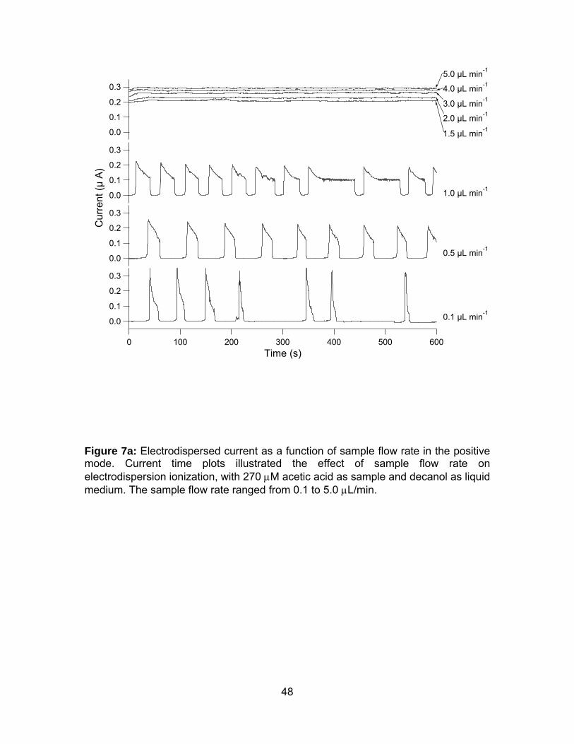
48

0.3

0.2

0.1

0.0

6005004003002001000Time (s)

0.3

0.2

0.1

0.0

0.3

0.2

0.1

0.0

Cur

rent

(µ A

)

0.3

0.2

0.1

0.0

0.1 µL min-1

0.5 µL min-1

1.0 µL min-1

2.0 µL min-13.0 µL min-14.0 µL min-1

1.5 µL min-1

5.0 µL min-1

Figure 7a: Electrodispersed current as a function of sample flow rate in the positive mode. Current time plots illustrated the effect of sample flow rate on electrodispersion ionization, with 270 μM acetic acid as sample and decanol as liquid medium. The sample flow rate ranged from 0.1 to 5.0 μL/min.

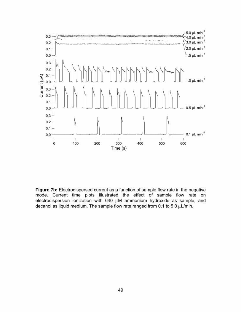
49

0.3

0.2

0.1

0.0

6005004003002001000Time (s)

0.3

0.2

0.1

0.0

0.3

0.2

0.1

0.0

Cur

rent

(µA)

0.3

0.2

0.1

0.0

0.1 µL min-1

0.5 µL min-1

1.0 µL min-1

1.5 µL min-1

2.0 µL min-13.0 µL min-14.0 µL min-15.0 µL min-1

Figure 7b: Electrodispersed current as a function of sample flow rate in the negative mode. Current time plots illustrated the effect of sample flow rate on electrodispersion ionization with 640 μM ammonium hydroxide as sample, and decanol as liquid medium. The sample flow rate ranged from 0.1 to 5.0 μL/min.

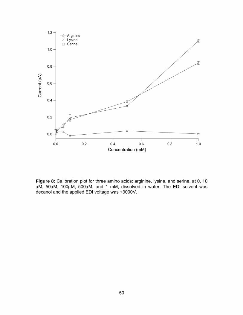
50

1.2

1.0

0.8

0.6

0.4

0.2

0.0

Cur

rent

(µA)

1.00.80.60.40.20.0Concentration (mM)

ArginineLysineSerine

Figure 8: Calibration plot for three amino acids: arginine, lysine, and serine, at 0, 10 μM, 50μM, 100μM, 500μM, and 1 mM, dissolved in water. The EDI solvent was decanol and the applied EDI voltage was +3000V.

51

Chapter Three

Liquid Phase Ion Mobility Spectrometry

Abstract

Aqueous phase analyte ions were extracted into and transported through a non-

electrolyte containing liquid to produce a novel analytical method, called liquid phase

ion mobility spectrometry. The movement of ions was directed by an electric field

established by using a series of metal rings connected with resistors. Spectra of

ammonium nitrate, sodium chloride, and fuchsin demonstrated liquid phase ion

mobility spectrometry. Although complex and inadequately resolved, these spectra

revealed that the ions could be transported and separated in an ion mobility

spectrometer operating in a liquid phase. Preliminary data with pulsed

electrodispersion ionization showed that a 5-mm long miniaturized liquid phase ion

mobility spectrometer had a resolving power of 17. By replacing the gas medium in

gas phase IMS with a non-electrolyte containing liquid medium, a miniaturized liquid

phase ion mobility spectrometer obtained a similar resolving power as a gas phase

IMS ten times its size.

52

Introduction

Interest in ion mobility spectrometry (IMS), first called plasma chromatography and

sometimes called ion chromatography or gas phase electrophoresis, expanded

exponentially in the last 15 years, as judged by the growth of IMS publications from

less than 20 per year in 1990 to over 135 per year in 2005. Ion mobility spectrometry

separates compounds based on the differences in mobilities in a weak electric field.

Ion mobilities depend on the size and charge of the ion as well as the interaction

between the ions and the separation medium. Reports have shown not only the

separation of isobaric analytes through their size-to-charge ratios in conventional ion

mobility spectrometry [1-5], but also the separation of enantiomers through their

different stereospecificities in chiral ion mobility spectrometry [6]. In addition, the

size-to-charge separation of IMS complements other separation techniques, such as

differential mobility spectrometry, mass spectrometry, and chromatography. Tandem

instruments with multidimensional separation modes were integrated for unraveling

complex metabolomes [7;8], protein structures [9;10] and carbohydrate identities [1].

The addition of IMS to other instruments can improve instrumental selectivity [11-13].

In an effort to increase the capabilities and separation efficiency of IMS, larger and

larger IMS instruments have been constructed. A record 210-cm long IMS drift tube

[14] and a tandem IMS-IMS drift tube of 182 cm in total length were introduced

recently [10]. The 210-cm long IMS was coupled to a quadrupole time-of-flight mass

spectrometer (QTOF MS). Lossless ion transmission from the mega long IMS to the

QTOF MS was made possible by an ion funnel whose inner diameter tapered

gradually [14]. Characterization of fragment ions were made possible by the two

53

staged IMS-IMS, where molecular ions underwent collisional activation after the first

stage of IMS [10].

In contrast to IMS instrument enlargement, much effort has also been spent on

miniaturizing IMS to capture its unique benefits of simple instrumentation and

milliseconds-fast analysis time [15-19]. Miniaturized IMS instruments have vast

applications, from medical, industrial, environmental, to military interests, as

personal chemical sensors for military personnel and first line responders [20;21],

building air quality sensors [22-24], and medical diagnostic sensors [25-27]. These

applications require compact, lightweight, and inexpensive analytical devices that

can also provide selective and sensitive monitoring in real-time. Unfortunately, most

miniaturized IMS instruments developed to date have significantly reduced resolving

powers relative to their larger counter parts. While resolving powers greater than 100

are common today for most large-scale IMS instruments, miniaturized instruments

exhibit resolving powers less than 30.

IMS resolution is not only dependent upon resolving power, but also upon

separation. Resolving power is a measure of the sharpness of a peak, while

separation is a measure of the difference in the average migration times of the

product ions of two analytes. Thus, the resolution (RS) between two analytes, with

reduced mobility values K0A and K0B, increase with the IMS resolving power:

0A 0BS P

0A

K - KR = 0.59R

K⎛ ⎞⎜ ⎟⎝ ⎠

(1)

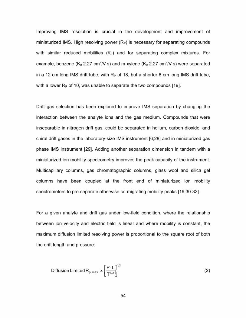
54

Improving IMS resolution is crucial in the development and improvement of

miniaturized IMS. High resolving power (RP) is necessary for separating compounds

with similar reduced mobilities (K0) and for separating complex mixtures. For

example, benzene (K0 2.27 cm2/V⋅s) and m-xylene (K0 2.27 cm2/V⋅s) were separated

in a 12 cm long IMS drift tube, with RP of 18, but a shorter 6 cm long IMS drift tube,

with a lower RP of 10, was unable to separate the two compounds [19].

Drift gas selection has been explored to improve IMS separation by changing the

interaction between the analyte ions and the gas medium. Compounds that were

inseparable in nitrogen drift gas, could be separated in helium, carbon dioxide, and

chiral drift gases in the laboratory-size IMS instrument [6;28] and in miniaturized gas

phase IMS instrument [29]. Adding another separation dimension in tandem with a

miniaturized ion mobility spectrometry improves the peak capacity of the instrument.

Multicapillary columns, gas chromatographic columns, glass wool and silica gel

columns have been coupled at the front end of miniaturized ion mobility

spectrometers to pre-separate otherwise co-migrating mobility peaks [19;30-32].

For a given analyte and drift gas under low-field condition, where the relationship

between ion velocity and electric field is linear and where mobility is constant, the

maximum diffusion limited resolving power is proportional to the square root of both

the drift length and pressure:

1 2

3 2p, maxP LDiffusion Limited RT⋅⎡ ⎤∝ ⎢ ⎥⎣ ⎦

(2)

55

Voltage and electric field do not play a role in the maximum diffusion limited

resolving power derivation because it is based on the notion that the highest electric

field under the low-field condition is used. It is apparent from equation (2) that

increasing the pressure of the medium would cancel out the negative effect of

miniaturization on separation efficiency of IMS. The extreme of increasing the

pressure of a gas will drive a phase transition and condense it into a liquid.

The objective of this project was to investigate the one parameter that had remained

consistent in the forty years of research in IMS – to replace the gaseous medium

with a liquid medium. Because of the low diffusion rates of analyte ions in liquids, it

should be able to miniaturize the instrumentation for liquid phase ion mobility

spectrometry (LPIMS) without concomitant loss in resolving power.

Although gas phase IMS has been called gas phase electrophoresis, LPIMS is

different from liquid phase electrophoresis. Like electrophoresis, ions in LPIMS

migrate under the influence of an electric field. While the electric field in

electrophoresis is established by the charged electrolyte in the liquid medium,

LPIMS does not require the presence of charged electrolyte. In LPIMS, the

spectrometer has decreasing potential with length that establishes an external

electric field. Because the liquid media in LPIMS contain no electrolyte, the only ion

current is carried by the ions produced in the ionization source. Hence, a universal

Faraday plate can be used to detect the ion current from the analyte. Besides the

advantage of offering a simple detection method, the lack of electrolyte in the liquid

medium permits the use of higher voltage in LPIMS without experiencing

degradation of resolving power due to joule heating.

56

Research of ion mobility in liquid phases began in the early 20th century as a series

of physical experiments evolving from conductivity studies of dielectric liquids. The

liquid media studied were liquid hydrocarbons, insulating oils and liquefied noble

gases. Bialobrzeski and Jaffé conducted the first experiments of mobility

measurements in dielectric liquids. Bialobrzeski [33] worked on the relation between

ion mobility and the viscosity (η) of the dielectric liquid medium in 1911 and Jaffé

[34] performed ion mobility experiments in hexane in 1913. In 1937, Adamczewski

[35] performed the first systematic ion mobility experiments in a series of liquid

saturated hydrocarbons and studied the relation of ion mobility to the coefficient of

viscosity. Adamczewski concluded that the mobility (μ) of ion was inversely

proportional to η3/2 at constant temperature, known as the Adamczewski’s relation. In

the 1950s, measurements of mobility of helium ions in liquefied helium were done by

Williams [36], L. Meyer et al [37], Careri et al [38] and Atkins [39]. In 1964, Gzowski

[40] measured mobility of positive and negative ions in pure and mixtures of

hydrocarbons. Although the ions were not identified, he concluded that (1) positive

ions of different mobilities were present; (2) mobility of negative ions were greater

that that of positive ions in all the liquids studied; (3) mobility of negative ions were

found to be inversely proportional to viscosity of liquid, known as the Walden’s Rule;

and (4) mobility of positive ions were found to be inversely proportional to η3/2, same

as Adamczewski’s finding in 1937.

Interests in mobility studies of dielectric liquids persisted. A majority of which

consisted of the physical investigations of positive and negative intrinsic ions of the

dielectric liquids in the study of the breakdown process of dielectric liquids [41-43],

57

the study of ion recombination and diffusion in liquids subjected to high-energy

radiation [44;45], and the study of dielectric liquid properties in particle counters and

spark chambers [46;47]. Investigations of ions from extrinsic analyte were less

studied. Examples were the analyses of sulfur hexafluoride [48], methyl halides [48],

tetramethylparaphenylenediamine [49;50], quinones [50;51], porphines [50;51], and

fullerenes [50;52]. In these instances, the samples were dissolved in the same

dielectric liquid medium where experiments were conducted. Up to this date, there

has been no research performed on using ion mobility spectrometry in liquid phases

as an analytical separation technique for aqueous phase analytes.

For the application of liquid phase ion mobility to analytical chemistry, however,

analyte ions, typically in aqueous samples, need to be introduced into the liquid

medium and transported through it in order to measure their mobilities. This paper

presents the concept of a chemical separation and analysis method based on ion

mobility spectrometry using a liquid phase instead of a gas phase as the medium

through with analyte ions migrate. LPIMS, on a miniaturized scale, is a novel

analytical separation method that is capable of achieving better separation power

than a gas phase IMS of the same dimension.


Instrumentation. Resistive Glass LPIMS. The apparatus consisted of an

electrodispersion ionization source (EDI), a mobility tube, and a Faraday plate

(Figure 1). The apparatus was placed inside a Pyrex dish (10 cm o.d. and 5 cm

58

height) filled with the liquid medium. The ion mobility tube was a resistive glass tube

(Burle Technologies Inc., Lancaster, PA) with a 4.1 mm i.d., 5.4 mm o.d., and 5 mm

in length. The internal surface resistance was 10 MΩ and the external surface

resistance was discontinued. Electrodes were attached to either ends of the resistive

glass tube. Voltage was applied to the front electrode. The end electrode was

grounded through a 430-kΩ resistor.

The aqueous sample of 10 μM basic fuchsin was delivered through a fused silica

capillary by a syringe pump (Pump 11 Plus, Harvard Apparatus, Holliston, MA) at 0.5

μL/min. A polyetheretherketone (PEEK) microelbow junction (Upchurch Scientific In.,

Oak Habor, WA) was used to allow a 90° bend of the fused silica capillary. The end

of the fused silica capillary was positioned approximately 2 mm in front of the ion

mobility tube. The EDI voltage, applied to a metal union, was set at 2000 V above

the ion mobility tube voltage. For example, when the voltage applied to the ion

mobility tube was 500 V, then the EDI voltage was 2500 V. The aqueous sample

was electrodispersed into the liquid medium and transported through the ion mobility

tube by the applied electric field. Total ion current was measured on the Faraday

plate, located 2.3 mm behind the resistive glass tube. The signal was amplified at

109 volts per ampere by a Keithley 427 current amplifier (Keithley Instruments,

Cleveland, OH) and acquired by a LabView (National Instruments, Austin, TX) based

data acquisition system. The mobility experiments were carried out in hexane while

varying the electric field on the ion mobility tube from 0 to 6000 V/cm. The

experiments were repeated with electrospray ionization (ESI) in air for comparison.

In order to establish the background current level in the two media, experiments

59

were also run with voltages applied to the ion mobility tube, but in the absence of

sample ionization.

The gating efficiency of Bradbury-Nielsen shutter was examined using an extended

variation of the above instrumentation, where the Bradbury-Nielsen shutter was

placed between two lengths of resistive glass tube of the same dimension. The

Bradbury-Nielsen shutter was constructed from two Macor ceramic rings with 4.56

mm i.d., 9.30 mm o.d., and a thickness of 2.26 mm. Alloy 46 stainless steel wires of

76 μm diameter (California Fine Wire Company, Grover Beach, CA) were wound at

0.64 mm parallel spacing. The shutter wires were sandwiched between the two

Macor rings and secured with a ceramic adhesive (Resbond 940, Cotronics Corp.,

Brooklyn, NY). Alternate wires on the Bradbury-Nielsen shutter were electrically

insulated, such that this would create an electrical field, orthogonal to the electric

field on the ion mobility spectrometer, when a potential was applied across these

alternate wires. The pulsing of the ion shutter was controlled by a Double Pole

Single Throw (DPST) two-way switch, constructed by Technical Services of

Washington State University.

Stacked-Ring LPIMS. Preliminary LPIMS data was obtained from an enclosed liquid

mobility spectrometer constructed at Washington State University (Figure 2). The ion

mobility spectrometer was produced by hollowing out half-cylinders from two Teflon

blocks. Slits for conducting electrodes were cut into the Teflon block at 1-mm apart.

Stainless steel electrodes (Fotofab, Chicago IL) were inserted into each slit. While

keeping each of the sixteen electrodes vertically aligned, the two Teflon blocks were

60

carefully combined and physically sealed by nylon screws at each of the four

corners. The ion mobility spectrometer had a 5 mm i.d. and a length of 20 mm. The

dimensions of this LPIMS were chosen to be a 1:10 model of the current gas phase

IMS in the Hill Research Lab. Liquid medium of mineral oil was pumped into the IMS

tube at the entry and exit, labeled as (D) and (E) in Figure 2. Aqueous samples were

introduced into the IMS tube through a fused silica capillary with a stainless steel

sleeve. The EDI voltage was applied to the stainless steel sleeve. The electrodes

were connected externally in series with 1-MΩ resistors. With 1000 V applied to the

first electrode, the electric field of the mobility tube was 482 V/cm.

In order to time the arrival of ions at the Faraday plate, a Tyndall ion shutter was

used [53]. A photo-etched gate electrode, with parallel wires 0.14 mm wide and 0.46

mm spacing, was positioned at the sixth electrode. To close the shutter, the voltage

of the gate electrode was electrically shorted to the eighth electrode to form a

potential well that stopped the ions from migrating forward. To open the shutter, the

voltage of the gate electrode was switched back to its normal voltage, in line with the

resistor series, allowing ions to migrate forward.

For the ammonium nitrate experiment, an aqueous solution of 2.8 mM ammonium

nitrate was injected into the LPIMS at 0.25 μL/min. +3000V was applied to the first

electrode with an electric field of +1714 V/cm. The voltage on the gate electrode was

+2100 V. The ion shutter pulse width was 5 s. For the sodium chloride experiment,

an aqueous solution of 2.2 mM of sodium chloride was delivered at 1 μL/min. The

61

EDI voltage was +1000V. The voltage on the gate electrode was measured to be

+684 V and the electric field was +558 V/cm. A faster gate pulse of 0.2 s was used.

The effectiveness of the Tyndall shutter was examined in this apparatus with the

upper Teflon block removed, due to a leakage problem. The LPIMS was placed

inside a Pyrex dish filled with hexane. The spectrometer had a total length of 29.5

mm and an electric field of 1695 V/cm. Methanol-water (90:10, vol/vol), with flow rate

of at 0.1 μL/min, was ionized by an EDI voltage of +6000V.

Materials and Reagent. The liquid media used in these experiments were hexane

(J. T. Baker, Phillipsburg NJ) and USP grade mineral oil (Penreco, Karns City PA).

10 μM basic fuchsin (4-((4-amino-3-methylphenyl)(4-

aminophenyl)methylene)cyclohexa-2,5-dieniminium chloride) and 1 μM

tetraethylammonium bromide (Sigma-Aldrich, St. Louis, MO) were both prepared in

methanol-water (90:10, vol/vol). 2.8 mM of ammonium nitrate (Fisher Scientific, Fair

Lawn NJ) and 2.2 mM of sodium chloride (JT Baker, Phillipsburg NJ) were prepared

in methanol-water (50:50, vol/vol). The methanol solvent used was HPLC grade (JT

Baker, Phillipsburg NJ). The 18.1 MΩ water used was ultra-purified with a water

purification system (Barnstead Int., Dubuque, IA).

62

Results and Discussions

Ion transmission through non-electrolyte containing liquids. The initial objective

was to demonstrate that ions can travel through a non-electrolyte containing liquid

under the influence of an electric field. The experiments were conducted in the

apparatus shown in Figure 1, with hexane as the liquid medium. Ions were

generated in hexane from a 10 μM aqueous solution of fuchsin by placing a high

voltage on a capillary in which an aqueous sample was flowing into the hexane at a

rate of 0.5 μL/min. In a manner similar to electrospray ionization, small charged

droplets of aqueous sample in hexane were generated through Coulombic repulsion.

This ionization process has been called electrodispersion ionization (EDI)[54].

Current in the apparatus was measured with the electric field of the mobility tube

varied from 0 to 6000 V/cm. For comparison between EDI and its gas phase

analogue, electrospray ionization (ESI), the experiments were conducted in air. The

same aqueous sample was ionized by ESI for the same range of IMS electric field.

The ionized sample traveled through the mobility tube in the respective medium. The

experiments were also repeated without sample ionization to establish the

background current level.

The background current levels in hexane and air were quite similar. At 5000 V/cm,

the background current in hexane was 4 pA, with a noise level of ±7 pA; and the

background current in air was 1 pA, with a noise level of ±4 pA. While there were

arcing between the two electrodes attached to the resistive glass tube at 5000 V/cm

63

in air, there was no arcing in hexane. However, gas bubbles could be observed at an

electric field of 6500 V/cm and above in hexane, possibly due to electrochemical

oxidation of impurities in hexane.

Results showed that the electrodispersed ion moved along an ion mobility

spectrometer in the non-electrolyte containing hexane under the influence of an

electric field. Furthermore, the total ion current increased with the electric field of the

mobility tube for both EDI in hexane and for ESI in air (Figure 3a). The total EDI

current reached a maximum of 1.4 nA at 6000 V/cm and the ESI current reached a

maximum of 1.2 nA at 4500 V/cm. Figure 3b showed that ionization and ion transport

efficiency also increased with the electric field. The efficiency leveled off at 15% for

an electric field of 4000V/cm and above.

Effectiveness of Ion Shutters in the Liquid Phase. Prior to conducting liquid

phase ion mobility experiments. Bradbury-Nielsen shutter and Tyndall shutter were

evaluated in the liquid phase. The electric field of the LPIMS was 600 V/cm and

1695 V/cm used in the examination of Bradbury-Nielsen shutter and Tyndall shutter,

respectively. Figure 4a and b showed the percentage of the total ion current stopped

by the Bradbury-Nielsen shutter and the Tyndall shutter, respectively, in hexane.

The Bradbury-Nielsen shutter was able to stop 90% of the ions at an orthogonal field

of 6000 V/cm (10 times the electric field of the LPIMS) and it was able to stop 95% of

the ions at an orthogonal field of 11100V/cm (18.5 times the electric field of the

LPIMS) (Figure 4a). These results suggested that an effective Bradbury-Nielsen

shutter would require an orthogonal field of 19000V/cm (32 times the electric field of

64

the LPIMS). Unfortunately, at higher orthogonal fields, noise increased and arcing

between the gate wires occurred.

The maximum reverse field of obtainable on the Tyndall shutter was13690 V/cm,

which was 8 times greater than the electric field of the LPIMS, stopped 95% of the

total ion current (Figure 4b). This suggested that a reverse field of 14260V/cm, or 8.5

times greater than the forward mobility field, would be sufficient in stopping the ions

from migrating further.

To further evaluate the effectiveness of the Tyndall shutter, ion current from

electrodispersed samples was measured while the shutter was held in the closed

position for the first 10 s, and then opened for the following 10 s of the spectrum.

The samples analyzed were 10 μM basic fuchsin, 1 μM tetraethylammonium

bromide, and the methanol-water sample blank. Figure 5 showed that substantial

current was registered for the three samples when gate was opened, compared to

when gate was close. The current measured for the sample blank was 8.2 ± 0.7 pA,

24.5 ± 0.8 pA for fuchsin, and 27.6 ± 0.9 pA for tetraethylammonium bromide. Gate

pulse ringing was registered at 0 s and 10 s when the ion shutter closed and

opened. After the ion shutter closed, the current decayed to zero in 5 s. This was the

time required for the ions remaining in the spectrometer from the previous

experiment to reach the detector. After the ion shutter opened, there was a delay

between 1.5 s to 2.0 s before the current rose. This time delay was the time the ions

required to travel from the ion shutter to the Faraday plate, or their mobility time.

65

Gated liquid phase ion mobility spectrometry. LPIMS spectra were obtained by

introducing short pulses of ions through the Tyndall ion shutter, using the apparatus

depicted in Figure 2, in mineral oil. The ion shutter pulse width was 5 s. The positive

LPIMS spectrum of 2.8 mM of ammonium nitrate, at a flow rate of 0.25 μL/min,

showed a prominent current signal (Figure 6, black). The complexity of the

ammonium nitrate spectrum indicated that the ions had not been completely

desolvated. The two most intense peaks, at 10.1 s and 42.9 s, had mobility values of

2.1 10-4 cm2/Vs and 5.0 10-5 cm2/Vs, respectively. The mobility value of

ammonium ions in water is 7.6 10-4 cm2/Vs [55]. With a viscosity of 57 cP, the

mineral oil is about 60 times more viscous than water. The ion mobility is inversely

proportional to the viscosity of the medium and hence the ion mobility in mineral oil

should be 60 times slower than that in water. The expected mobility of ammonium

ion in mineral oil would be 1.3 10-5 cm2/Vs. The experimental mobility values were

4 and 16 times faster than expected. Although this spectrum was noisy and relatively

low resolution, it showed that LPIMS is achievable and possible.

The ion shutter pulse width was shortened to 0.2 s in the subsequent experiment to

reduce peak broadening. The background spectrum in the absence of sample was

shown in blue (Figure 7). The positive LPIMS spectrum of sodium chloride in Figure

7 (black spectrum) was less complex than the ammonium nitrate spectrum and

showed a signal peak at 15.6 s with a mobility of 1.4 10-4 cm2/Vs. The literature

value of ion mobility of sodium ion in water of 5.2 10-4 cm2/Vs [55] and the

expected mobility of Na+ in mineral oil is 8.7 10-6 cm2/Vs. The experimental ion

mobility value of 1.4 10-4 cm2/Vs was 16 times faster than anticipated.

66

Preliminary demonstration of pulsed EDI-LPIMS. Electrodispersion ionization

source was operated in a pulse mode, using the apparatus depicted in Figure 1. No

ion shutter was used. The pulsed injection of ions was controlled by alternating the

EDI voltage between a voltage sufficient to induce ionization (+2000V) and a lower

voltage (+500V). The EDI voltage was maintained at the upper voltage for 0.5 s, and

switched to the lower voltage for the remaining of the experiment.

Figure 8 showed the pulsed EDI-LPIMS spectrum of 10 μM basic fuchsin, at a flow

rate of 0.1 μL/min, drifting in hexane at an electric field of 978 V/cm. The spectrum in

full scale was displayed, as an insert in Figure 8, to show the voltage ringing from

the ionization pulse at 0 s and 0.5 s. The pulsed injection of ions significantly

reduced the spectrum complexity in comparison with the gated spectra. Because

ions were only introduced during the ionization pulse, there were no additional

aqueous analyte injected into the spectrometer while the mobility data was collected.

A single peak was observed for basic fuchsin at a drift time of 1.01 s and a mobility

of 2.72 10-3 cm2/V⋅s. The peak width was 0.06 s, which was shorter than the 0.5 s

ionization pulse. This suggested that at a low sample flow rate, the sample was

ejected at a faster rate than it was being delivered. The LPIMS had a resolving

power of 17.

This resolving power was better than several gas phase IMS that were 8 to 12 times

longer [18;19;56]. The resolving power per unit drift length of miniature gas phase

IMS ranged from 1.1 cm-1 to 7.7 cm-1 [18;19;56-58]. The resolving power per unit drift

length of this 5-mm LPIMS was 34 cm-1.

67

Conclusions

This first demonstration of liquid phase ion mobility spectrometry, with

electrodispersion ionization, introduces the concept of a new analytical separation

technique on a miniature scale. Aqueous ions are moved along the LPIMS by an

electric field, established by conducting electrodes held at decreasing potentials, in a

non-electrolyte containing liquid medium. The ion transport efficiency of LPIMS

improves linearly with the applied electric field of the spectrometer. The gate injected

LPIMS spectra are inadequately resolved, due to the extension of solvation and the

inefficiency of the ion shutters. While further approaches are necessary to assist

sample desolvation and to improve gating of ions, pulsed EDI-LPIMS data

demonstrated LPIMS as a promising novel analytical technique for the liquid phase.

Acknowledgements



68

References

1. B. H. Clowers, B. Bendiak, P. Dwivedi, W. E. Steiner and Jr. H. H. Hill, Separation of Sodiated Isobaric Disaccharides Using Electrospray Ionization-Atmospheric Pressure Ion Mobility-Time of Flight Mass Spectrometry, Journal of the American Society for Mass Spectrometry 16 , pp. 660-669 (2005).

2. S. N. Jackson, H. Y. N. Wang and A. S. Woods, Direct Tissue Analysis of Phospholipids in Rat Brain Using MALDI-TOFMS and MALDI-Ion Mobility-TOFMS, Journal of the American Society for Mass Spectrometry 16, pp. 133-138 (2005).

3. C. A. Srebalus, J. W. Li., W. S. Marshall and D. E. Clemmer, Gas Phase Separations of Electrosprayed Peptide Libraries, Analytical Chemistry 71, pp. 3918-3927 (1999).

4. G. R. Asbury and Jr. H. H. Hill, Separation of Amino Acids by Ion Mobility Spectrometry, Journal of Chromatography A 902, pp. 433-437 (2000).

5. C. S. Creaser and J. R. Griffiths, Atmospheric Pressure Ion Mobility Spectrometry Studies of Cyclic and Acyclic Polyethers, Analytica Chimica Acta 436, pp. 273-279 (2001).

6. P. Dwivedi, C. Wu and Jr. H. H. Hill, Gas Phase Chiral Separations by Ion Mobility Spectrometry, Analytical Chemistry ASAP DOI: 10.1021/ac0608772 (2006).

7. V. Ruzsanyi, J. I. Baumbach, S. I. Sielemann, P. Litterst, M. Westhoff and L. Freitag, Detection of human metabolites using multi-capillary columns coupled to ion mobility spectrometers, Journal of Chromatography A 1084, pp. 145-151 (2005).

8. P. Wu, P. Dwivedi, S. J. Klopsch, G. J. Puzon, L. Xun and Jr. H. H. Hill, Metabolic Profiling by Ion Mobility Mass Spectrometry (IMMS), Manuscript in Preparation, (2006).

9. S. I. Merenbloom , S. L. Koeniger, S. J. Valentine, M. D. Plasencia and D. E. Clemmer, IMS-IMS and IMS-IMS-IMS/MS for Separating Peptide and Protein Fragment Ions, Analytical Chemistry 78, pp. 2802-2809 (2006).

10. S. L. Koeniger, S. I. Merenbloom, S. J. Valentine, M. F. Jarrold, H. R. Udseth, R. D. Smith and D. E. Clemmer, An IMS-IMS Analogue of MS-MS, Analytical Chemistry 78 , pp. 4161-4174 (2006).

11. D. A. Atkinson, Jr. H. H. Hill and T. D. Shultz, Quantification of Mammalian Lignans in Biological-Fluids Using Gas-Chromatography with Ion Mobility

69

Detection, Journal of Chromatography-Biomedical Applications 617, pp. 173-179 (1993).

12. B. T. Ruotolo, G. F. Verbeck, L. M. Thomson, A. S. Woods, K. J. Gillig and D. H. Russell, Distinguishing between Phosphorylated and Nonphosphorylated Peptides with Ion Mobility-Mass Spectrometry, Journal of Proteome Research 1, pp. 303-306 (2002).

13. L. M. Matz, H. M. Dion and Jr. H. H. Hill, Evaluation of Capillary Liquid Chromatography-Electrospray Ionization Ion Mobility Spectrometry with Mass Spectrometry Detection, Journal of Chromatography A 946, pp. 59-68 (2002).

14. K. Tang, A. A. Shvartsburg, H-N Lee, D. C. Prior, M. A. Bauschbach, F. Li, A. V. Tolmachev, G. A. Anderson and R. D. Smith, High-Sensitivity Ion Mobility Spectrometry/Mass Spectrometry Using Electrodynamic Ion Funnel Interfaces, Analytical Chemistry 77, pp. 3330-3339 (2005).

15. J. Xu, W. B. Whitten, T. A. Lewis and J. M. Ramsey, A Miniature Ion Mobility Spectrometer with a Pulsed Corona-Discharge Ion Source, International Journal for Ion Mobility Spectrometry 4 , pp. 3-6 (2001).

16. J. I. Baumbach, D. Berger, J. W. Leonhardt and D. Klockow, Ion Mobility Sensor in Environmental Analytical Chemistry -- Concept and First Results, Intern. J. Environ. Anal. Chem. 52, pp. 189-193 (1993).

17. J. Xu, W. B. Whitten and J. M. Ramsey, Pulsed-Ionization Miniature Ion Mobility Spectrometer, Analytical Chemistry 75, pp. 4206-4210 (2003).


19. St. Sielemann, J. I. Baumbach, H. Schmidt and P. Pilzecker, Quantitative Analysis of Benzene, Toluene, and m-Xylene with the Use of a UV-Ion Mobility Spectrometer, Field Analytical Chemistry and Technology 4, pp. 157-169 (2000).

20. J. P. Carrico, A. W. Davis, D. N. Campbell, J. E. Roehl, G. R. Sima, G. E. Spangler, K. N. Vora and R. J. White, Chemical Detection and Alarm for Hazardous Chemicals Using Ion Mobility Instrumentation, American Laboratory 18, p. 152 (1986).

21. D. D. Fetterolf and T. D. Clark, Detection of Trace Explosive Evidence by Ion Mobility Spectrometry, Journal of Forensic Science 38, pp. 28-39 (1993).

22. Z. Karpas, Y. Pollevoy and S. Melloul, Determination of Bromine in Air by Ion Mobility Spectrometry, Analytica Chimica Acta 249, pp. 503-507 (1991).

23. H. R. Bollan, D. J. West and J. L. Brokenshire, Assessment of Ion Mobility Spectrometry for Monitoring Monoethanolamine in Recycled Atmospheres,

70

International Journal for Ion Mobility Spectrometry 1, pp. 48-53 (1998).

24. G. Gordon, G. Pacey, B. Bubnis, S. Laszewski and J. Gaines, Safety in the Workplace: Ambient Chlorine Dioxide Measurements in the Presence of Chlorine, Chemical Oxidation 4, pp. 23-30 (1997).

25. J. P. Dworzanski, W. H. McClennen, P. A. Cole, S. N. Thorton, H. L. C. Meuzelaar, N. S. Arnold and A. P. Snyder, Field-Portable, Automated Pyrolysis-GC/IMS System for Rapid Biomarker Detection in Aerosols: a Feasibility Study, Field Analytical Chemistry and Technology 1, pp. 295-305 (1997).

26. V. Ruzsanyi, S. Sielemann and J. I. Baumbach, Determination of VOCs in Human Breath Using IMS, International Journal for Ion Mobility Spectrometry 5, pp. 45-48 (2002).

27. Z. Karpas, W. Chaim, B. Tilman, R. Gdalevsky and A. Lorber, A Diagnosis of Vaginal Infections by Ion Mobility Spectrometry, International Journal for Ion Mobility Spectrometry 5, pp. 49-54 (2002).

28. L. M. Matz and Jr. H. H. Hill, Investigation of Drift Gas Selectivity in High Resolution Ion Mobility Spectrometry with Mass Spectrometry Detection, Journal of the American Society for Mass Spectrometry 13, pp. 300-307 (2002).

29. A. B. Kanu and H. H. Hill, Jr. Drift Gas Selectivity with Thermal Desorption Ion Mobility Spectrometry. Gordon Research Conference. 2005.

30. S. Sielemann, J. I. Baumbach, P. Pilzecker and G. Walendzik, Detection of trans-1,2-dichloroethene, trichloroethene and tetrachloroethene using Multi-Capillary Columns Coupled to Ion Mobility Spectrometers with UV-Ionization Sources, International Journal for Ion Mobility Spectrometry 2, pp. 15-21 (1999).

31. A. B. Kanu, C. Wu, and H. H. Hill, Jr. Rapid Pre-Separation for Eliminating False Positive Interferences from Drugs, Explosives and Chemical Warfare Agents in Ion Mobility Spectrometry. Gordon Research Conference. 2005.

32. A. P. Snyder, C. S. Harden, A. H. Brittain, M. G. Kim, N. S. Arnold and H. L. C. Meuzelaar, Portable Hand-Held Gas-Chromatography Ion Mobility Spectrometry Device, Analytical Chemistry 65, pp. 299-306 (1993).

33. C. Bialobrzeski, Le Radium 8, p. 1 (1911).

34. G. Jaffé, Über die Ionisation flüssiger Dielektrika durch Radiumstrahlen, Annalen der Physik 330, pp. 257-284 (1908).

35. I. Adamczewski, Mobilités des Ions dans la Série des carbures d'Hydrogčne Liquides et Leur Rapport avec le Coefficient de Viscositč, Annls de Physique 8, pp. 309-359 (1937).

71




39. K. R. Atkins, Ions in Liquid Helium, Physical Review 116, pp. 1339-1343 (1959).

40. O. Gzowski, Mobility of Ions in Liquid Dielectrics, Nature 194, p. 173 (1962).

41. J. A. Kok, Electrical Breakdown of Insulating Liquids. Interscience Publishers, New York (1961).

42. M. J. Morant, Photo-Injection of Charge into Dielectric Liquids, Nature (London) 187, pp. 48-49 (1960).

43. A. M. Sletten, Electric Strength and High-Field Conduction Current in n-Hexane, Nature (London) 183, pp. 311-312 (1959).

44. G. Jaffé, Zur Theorie der Ionisation in Kolonnen, Annalen der Physik 347, pp. 303-344 (1913).

45. J. F. Fowler and F. T. Farmer, Conductivity Induced in Unplasticized 'Perspex' by X-rays, Nature (London) 175, pp. 516-517 (1955).

46. H. J. Plumley, Conduction of Electricity by Dielectric Liquids at High Field Strengths, Physical Review 59, pp. 200-207 (1941).

47. I. Adamczewski, Liquid-filled Ionization Chambers as Dosimeters, Colloques Internationaux du Centre National de la Recherche Scientifique 179, pp. 21-44 (1970).

48. A. O. Allen, M. P. Haas and A. Hummel, Measurement of Ionic Mobilities in Dielectric Liquids by Means of Concentric Cylindrical Electrodes, Journal of Chemical Physics 64, pp. 2587-2592 (1976).

49. N. Houser and R. C. Jarnagin, Electron Ejection from Triplet State in Fluid Solutions, Journal of Chemical Physics 52, pp. 1069-1078 (1970).

50. S. K. Lim, M. E. Burba and A. C. Albrecht, Mobilities of Radical Cations and Anions, Dimer Radical Anions, and Relative Electron Affinities by Times of Flight in n-hexane, Journal of Physical Chemistry 98, pp. 9665-9675 (1994).

51. K. S. Haber and A. C. Albrecht, Time-of-Flight Technique for Mobility Measurements in the Condensed Phase, Journal of Physical Chemistry 88, pp.

72

6025-6030 (1984).

52. M. E. Burba, S. K. Lim and A. C. Albrecht, Relative Electron Affinity of C60 and C70 and the Stokes' Law Radius of the C70 Radical Anion in n-Hexane by Time-of-Flight Mobility Measurements, Journal of Physical Chemistry 99, pp. 11839-11843 (1995).

53. A. M. Tyndall, The Mobility of Positive Ions in Gases. Cambridge University Press, Cambridge, U.K. (1938).

54. M. Tam and H. H. Hill, Jr. Electrodispersion Ionization in Liquids, Submitted (2006).

55. A. P. Snyder, C. S. Harden, A. H. Brittain, M-G Kim, N. S. Arnold and H. L. C. Meuzelaar, Portable Hand-Held Gas Chromatography/Ion Mobility Spectrometry Device, Analytical Chemistry 65, pp. 299-306 (1993).


57. J. I. Baumbach, S. Sielemann and P. Pilzecker, Coupling of Multi-Capillary Columns with two Different Types of Ion Mobility Spectrometer, International Journal for Ion Mobility Spectrometry 3, pp. 28-37 (2000).

58. J. Xu, W. B. Whitten and J. M. Ramsey, Space Charge Effects on Resolution in a Miniature Ion Mobility Spectrometer, Analytical Chemistry 72, pp. 5787-5791 (2000).

73

Figure Captions

Figure 1: Schematic of the liquid phase resistive glass ion mobility tube. The

aqueous sample was ionized by the electrodispersion ionization source (A) into the

liquid medium, contained inside a Pyrex dish (B), and transported through the

resistive glass tube (C) by an electric field. The current was measured by the

Faraday plate (D).

Figure 2: Schematic of the enclosed stacked-ring liquid phase ion mobility

spectrometer. The units comprising the spectrometer were: (A) Teflon blocks, (B)

stainless steel electrodes, (C) Faraday plate, (D) liquid medium entry, (E) liquid

medium exit, and (F) sample inlet.

Figure 3: This plot showed the effect of the electric field of the ion mobility

spectrometer on (a) the total ion current and (b) the ionization and ion transport

efficiency of ESI in air and EDI in hexane. The background current levels in air and

hexane were shown for comparison in (a).

Figure 4: The effectiveness of (a) Bradbury-Nielsen shutter and (b) Tyndall shutter

in stopping ion current in liquid phase ion mobility spectrometry.

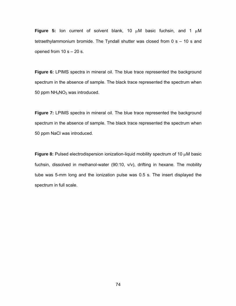
74

Figure 5: Ion current of solvent blank, 10 μM basic fuchsin, and 1 μM

tetraethylammonium bromide. The Tyndall shutter was closed from 0 s – 10 s and

opened from 10 s – 20 s.

Figure 6: LPIMS spectra in mineral oil. The blue trace represented the background

spectrum in the absence of sample. The black trace represented the spectrum when

50 ppm NH4NO3 was introduced.

Figure 7: LPIMS spectra in mineral oil. The blue trace represented the background

spectrum in the absence of sample. The black trace represented the spectrum when

50 ppm NaCl was introduced.

Figure 8: Pulsed electrodispersion ionization-liquid mobility spectrum of 10 μM basic

fuchsin, dissolved in methanol-water (90:10, v/v), drifting in hexane. The mobility

tube was 5-mm long and the ionization pulse was 0.5 s. The insert displayed the

spectrum in full scale.

75

Figure 1: Schematic of the liquid phase resistive glass ion mobility tube. The aqueous sample was ionized by the electrodispersion ionization source (A) into the liquid medium, contained inside a Pyrex dish (B), and transported through the resistive glass tube (C) by an electric field. The current was measured by the Faraday plate (D).

(A) Electrodispersion Ionization Source

(C) Resistive Glass Tube (D) Faraday Plate

(B) Pyrex Dish Filled with Liquid Medium

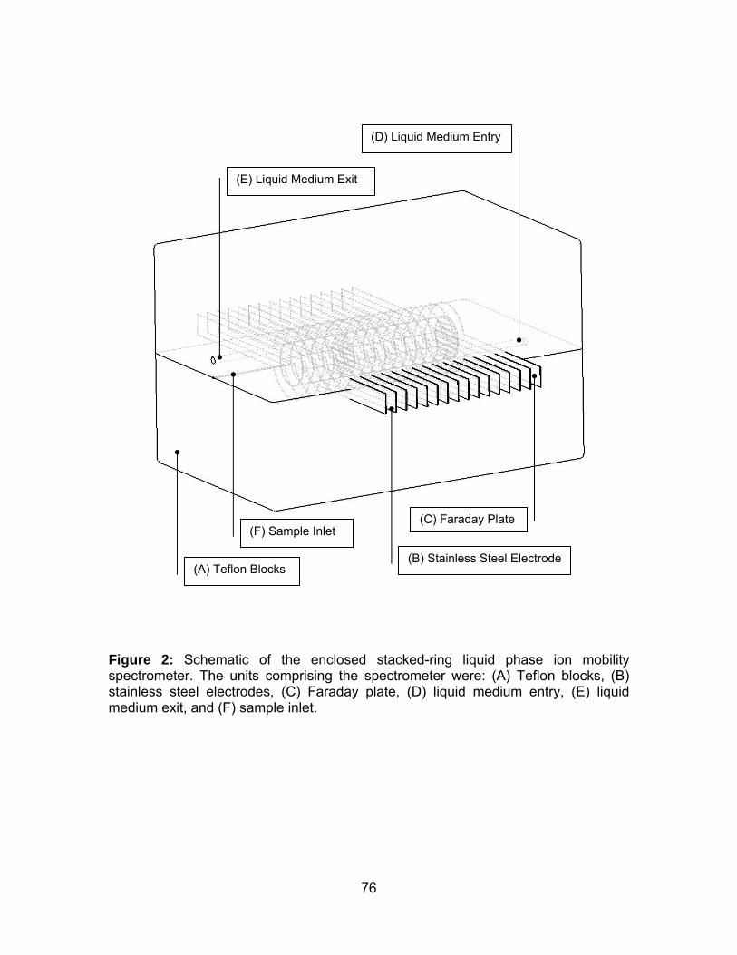
76

Figure 2: Schematic of the enclosed stacked-ring liquid phase ion mobility spectrometer. The units comprising the spectrometer were: (A) Teflon blocks, (B) stainless steel electrodes, (C) Faraday plate, (D) liquid medium entry, (E) liquid medium exit, and (F) sample inlet.

(C) Faraday Plate

(D) Liquid Medium Entry

(E) Liquid Medium Exit

(A) Teflon Blocks

(F) Sample Inlet

(B) Stainless Steel Electrode

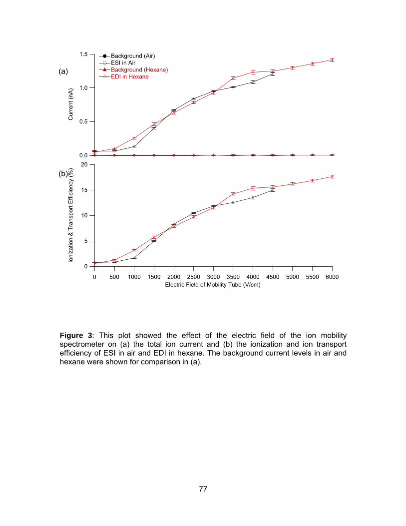
77

1.5

1.0

0.5

0.0

Cur

rent

(nA

)

600055005000450040003500300025002000150010005000Electric Field of Mobility Tube (V/cm)

20

15

10

5

0

Ioni

zatio

n &

Tra

nspo

rt E

ffici

ency

(%)

Background (Air)ESI in AirBackground (Hexane)EDI in Hexane

Figure 3: This plot showed the effect of the electric field of the ion mobility spectrometer on (a) the total ion current and (b) the ionization and ion transport efficiency of ESI in air and EDI in hexane. The background current levels in air and hexane were shown for comparison in (a).

(a)

(b)

78

100

80

60

40

20

0

% T

otal

Ion

Cur

rent

Sto

pped

175001500012500100007500500025000Orthogonal Electric Field (V/cm)

100

75

50

25

0

% T

otal

Ion

Cur

rent

Sto

pped

3500300025002000150010005000Depth of Potential Well (V)

Figure 4: The effectiveness of (a) Bradbury-Nielsen shutter and (b) Tyndall shutter in stopping ion current in liquid phase ion mobility spectrometry.

(a)

(b)

79

0.05

0.04

0.03

0.02

0.01

0.00

Cur

rent

(nA

)

20181614121086420Time (s)

Solvent blank10 µM basic fuchsin1 µM tetraethylammonium bromide

Figure 5: Ion current of solvent blank, 10 μM basic fuchsin, and 1 μM tetraethylammonium bromide. The Tyndall shutter was closed from 0 s – 10 s and opened from 10 s – 20 s.

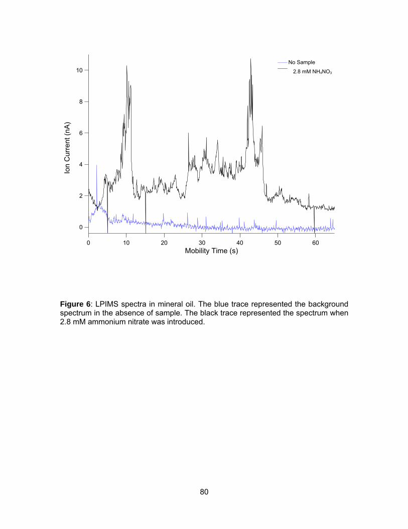
80

10

8

6

4

2

0

Ion

Cur

rent

(nA)

6050403020100Mobility Time (s)

No Sample50 ppm NH4NO3

Figure 6: LPIMS spectra in mineral oil. The blue trace represented the background spectrum in the absence of sample. The black trace represented the spectrum when 2.8 mM ammonium nitrate was introduced.

2.8 mM NH4NO3

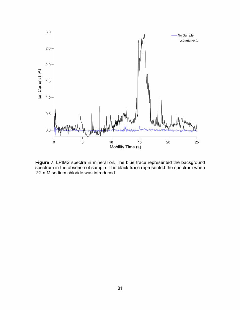
81

3.0

2.5

2.0

1.5

1.0

0.5

0.0

Ion

Cur

rent

(nA

)


No Sample50 ppm NaCl

Figure 7: LPIMS spectra in mineral oil. The blue trace represented the background spectrum in the absence of sample. The black trace represented the spectrum when 2.2 mM sodium chloride was introduced.

2.2 mM NaCl

82

0.20

0.15

0.10

0.05

0.00

-0.05

Cur

rent

(nA

)

5.04.03.02.01.00.0Mobility Time (s)

-1.5

-1.0

-0.5

0.0

0.5

1.0

1.5

Cur

rent

(nA)


Figure 8: Pulsed electrodispersion ionization-liquid mobility spectrum of 10 μM basic fuchsin, dissolved in methanol-water (90:10, v/v), drifting in hexane. The mobility tube was 5-mm long and the ionization pulse was 0.5 s. The insert displayed the spectrum in full scale. The spectrum was averaged 50 times.

83

Chapter Four

Design, Construction, and Evaluation of an

Integrated Liquid Phase Ion Mobility Spectrometer

Abstract

This paper presents two integrated miniaturized liquid phase ion mobility

spectrometry devices. Counterflow of liquid medium was necessary to remove

uncharged analyte in liquid phase ion mobility spectrometer. While this could not be

achieved in existing instruments, new designs were explored to address this

particular issue. In addition, alternative fabrication processes were considered in

terms of cost-effective mass production. Low temperature co-fired ceramics and

poly(dimethylsiloxane) are widely used in production of miniaturized and microfluidic

instruments. Liquid phase ion mobility spectrometers fabricated from these two

materials were evaluated based on the ability of liquid containment, electrical

integrity, and ion transport efficiency.

84

Introduction

Liquid phase ion mobility spectrometry (LPIMS) has recently been developed as a

novel analytical separation technique in the non-electrolyte containing liquids [1-3].

Liquid phase ions, produced from electrodispersion ionization (EDI) [4], are moved

along the spectrometer by an electric field. The electric field is established, not by

electrolytes in the liquid medium, but by multiple guard rings stationed along the

spectrometers.

The two existing designs for miniaturized LPIMS instrument. The first prototype was

an arrangement of guard rings sealed inside two pieces of Teflon block. It was a

1:10 model of the unidirectional stacked-ring gas phase ion mobility spectrometers

(IMS) in our laboratory. Half cylinders of 5-mm i.d. were hollowed out from two

Teflon blocks. The guard rings, inserted into slits of the Teflon blocks, were

connected in series by resistors and electrically insulated from one another. The two

Teflon blocks were sealed to form a liquid phase ion mobility spectrometer with an

i.d. of 5 mm and a length of 20 mm. An electric field was established by applying a

voltage to the first guard ring, and grounding the last guard ring through a resistor.

Ion signal were collected as a discharge current on a Faraday plate.

The second prototype utilized resistive glass tubes (Burle Technologies Inc.,

Lancaster, PA). Resistive glass tubes had been used in gas phase ion mobility

spectrometry in 1980s by Spangler [5;6]. Results obtained from the resistive coated

mobility tube were compared to those obtained from a conventional stacked-ring

85

mobility tube. It was found that while the resolving power was similar between the

two systems, the resistive coated mobility tube offered better sensitivity, possibly due

to the more uniform electric field in the resistive coated mobility tube [5]. The

resistive glass tubes (Burle) were fabricated from proprietary lead silicate glass,

which surface was converted to semi-conductor by reducing in hydrogen. The great

reduction in parts and assembly requirements were suitable for constructing

miniaturized LPIMS instrument. Individual guard rings, resistors, and their

connections, were replaced by a single piece of resistive glass tube. The resistive

glass LPIMS prototype had 4.1 mm i.d., 5.4 mm o.d., 5 mm length, and total

resistance of 8 MΩ to 10 MΩ. Electrodes were attached to either ends of the

resistive glass tube to provide electrical contact. The front electrode was used for

applying voltage to the spectrometer, while the end electrode was grounded via a

resistor.

Although the two existing prototypes demonstrated the feasibility of LPIMS, the

inherent design problems need to be addressed. The first prototype encountered

leakage problem. Subsequent LPIMS experiments were conducted by removing the

top Teflon block and immersing the prototype in a container of liquid medium.

Without proper containment, the second resistive glass LPIMS prototype were also

immersed in a container of liquid medium. Previous LPIMS results suggested the

need for a counterflow of liquid medium to remove uncharged analyte molecules

from the spectrometer (Chapter 5).

86

Low-temperature co-fired ceramic (LTCC), a type of ceramic sheet that was

frequently used in integrated microelectronic packaging, ceramic printed wiring

boards, and radiofrequency modules. LTCC comprises of alumina particles, lead

oxide and silicon dioxide glass particles, and proprietary organic binding compounds.

Before subjecting to high heat in a furnace, or the firing process, the LTCC sheet is

flexible and machineable. Electronic circuits can be printed onto the ceramic sheet

by applying conductive and resistive pastes. During the firing process, the organic

binder is burnt off, and glass and alumina fuse into a monolithic structure. This

process benefits miniaturization of ion mobility instruments because the electronic

circuits are printed embedded within the mobility tube, and eliminates the need for

external resistors. LTCC, with its breakdown voltage of 40 kV mm-1 and chemical

inertness, is suitable for the application of LPIMS. Much of the LTCC fabrication

process can be performed automatically by machines. Given the low cost of the

LTCC sheets, this would be a cost-effective way of mass-producing LPIMS devices.

Pfeifer et al explored LTCC as a potential solution for mass-producing miniaturized

gas phase IMS [7]. Their rolled design eliminated many parts by machine-printing

electrodes and resistors onto an unfired sheet of pliable low temperature co-fire

ceramic. The printed low temperature co-fire ceramic was rolled into the required

size. After subjected to high heat treatment, the rolled tube with the printed

electrodes and resistors fused with the ceramic into one piece. Only minimal manual

connections were required for this fabrication process.

Poly(dimethylsiloxane) (PDMS), also known as dimethicone, which had previously

been used to produce chip-based microfluidic systems for electrophoresis, DNA

sequencing, polymerase chain reaction, and immunoassays [8;9].The first capillary

87

zone electrophoresis on a PDMS chip was reported in 1997 by Effenhauser [10].

PDMS is a polymeric structure with repeating [SiO(CH3)2] monomeric units.

Polycarbonate and polymethylmethacrylate (PMMA) are two other polymeric

substrates that have been used for microfluidic systems. The unique properties of

PDMS make it suitable for preparing microfluidic devices. It is optically transparent

(down to 240 nm), gas permeable, water impermeable, flexible, and inexpensive. It

has low chemical reactivity, high dielectric strength (20 kV/mm), and a high operating

temperature range (-50 to 200°C). The viscoelasticity property of PDMS lends itself

to be useful as adhesives, lubricants, damping fluids, and heat transfer fluids. The

non-toxic, non-flammable, and biocompatible nature of PDMS have allowed its use

in other applications, including being used as an anti-caking agent by the food

industry, as an anti-foaming agent by the pharmaceutical industry, as knuckle

replacement implants and breast implants by the medical device industry. PDMS is

also suitable for constructing the ionization source. An electrospray ionization source

fabricated by PDMS was recently reported [11], where the hydrophobicity of PDMS

was stated to improve electrospray ionization by forming smaller Taylor cone from.

This suggested that integrating electrodispersion ionization source with LPIMS in a

single device would be viable.

The design objectives for an integrated LPIMS device should include all the requisite

components (an inlet for the electrodispersion ionization source, a liquid medium

inlet and outlet, insulated and contained housing, embedded electrodes and

resistors), with undemanding fabrication process, and have the capacity for mass

production and further miniaturization. This study presents the design and fabrication

88

of integrated miniaturized devices of LPIMS with LTCC and PDMS materials. The

devices were evaluated on basis of liquid containment, electrical integrity, and ion

transport efficiency.

Design and Fabrication of Integrated Liquid Phase Ion Mobility

Spectrometer

Design of Low Temperature Co-fired Ceramics LPIMS

The LPIMS ceramic device composed of the desolvation region, the ion shutter

region, the drift region, the aperture grid/Faraday plate region, and an insulating

base region. The mobility tube had a 3.8 mm i.d.. The LPIMS included 28 layers of

LTCC in the desolvation region, 5 layers in the gate region, 42 layers in the drift

region, 10 layers in the aperture grid/Faraday plate region, and 5 layers in the

insulating end region. This amounted to a total length of 18.1 mm, a drift length of

10.4 mm, and a total resistance of 5.8 MΩ. The design should provide a very

homogeneous electric field, having 50 electrodes per cm of drift length.

The obvious advantage of a LTCC device was the great reduction in electrical

connections. The electrodes and resistors were connected by vias and embedded

within the LTCC structure. The LTCC device had only five external connections for

grounding, sensing ion shutter reference voltage, delivering ion shutter voltage and

89

drift tube voltage, and outputting ion signal. These five connections were located on

the underside of the LTCC mobility tube.

The LTCC mobility tube was enclosed by three pieces of Teflon end caps. The first

and second pieces of Teflon end caps sandwiched a septum membrane that fitted

into the counter bore of the end cap. The fused silica capillary from EDI source was

introduced through this septum. The second and the third pieces of Teflon end caps,

located at either ends of the LTCC mobility tube, were sealed with two pieces o-

rings. The three pieces of Teflon end caps were tightened physically with three

screws. The third Teflon end cap supported five pogo pins, which pushed into the

five external electrical connectors on the underside of the mobility tube. The pogo

pins were connected to external electrical wire for inputting voltages, grounding, and

outputting signal. The schematic of the complete LTCC-LPIMS device was illustrated

in Figure 1, showing the position of the o-rings and septum within the device.

The LTCC (Green Tape 951, DuPont Microcircuit Materials, Research Triangle Park

NC) was intended for layering up to 30 sheets. Since a LPIMS would require 90

sheets of LTCC, LPIMS was constructed in multiple segments that were bonded with

pressure-sensitive adhesive to form the final mobility tube. In addition, the use of

multiple segments allowed for integration of external electrodes, such as ion shutter

and target screen, and for easy compilation of different mobility regions – the

desolvation, the Tyndall gate, the drift tube, and the aperture grid/faraday regions.

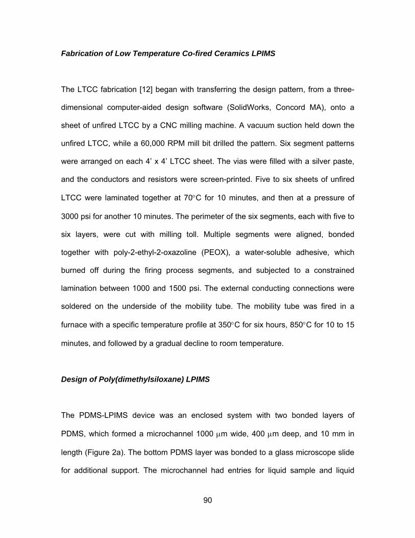
90

Fabrication of Low Temperature Co-fired Ceramics LPIMS

The LTCC fabrication [12] began with transferring the design pattern, from a three-

dimensional computer-aided design software (SolidWorks, Concord MA), onto a

sheet of unfired LTCC by a CNC milling machine. A vacuum suction held down the

unfired LTCC, while a 60,000 RPM mill bit drilled the pattern. Six segment patterns

were arranged on each 4’ x 4’ LTCC sheet. The vias were filled with a silver paste,

and the conductors and resistors were screen-printed. Five to six sheets of unfired

LTCC were laminated together at 70°C for 10 minutes, and then at a pressure of

3000 psi for another 10 minutes. The perimeter of the six segments, each with five to

six layers, were cut with milling toll. Multiple segments were aligned, bonded

together with poly-2-ethyl-2-oxazoline (PEOX), a water-soluble adhesive, which

burned off during the firing process segments, and subjected to a constrained

lamination between 1000 and 1500 psi. The external conducting connections were

soldered on the underside of the mobility tube. The mobility tube was fired in a

furnace with a specific temperature profile at 350°C for six hours, 850°C for 10 to 15

minutes, and followed by a gradual decline to room temperature.

Design of Poly(dimethylsiloxane) LPIMS

The PDMS-LPIMS device was an enclosed system with two bonded layers of

PDMS, which formed a microchannel 1000 μm wide, 400 μm deep, and 10 mm in

length (Figure 2a). The bottom PDMS layer was bonded to a glass microscope slide

for additional support. The microchannel had entries for liquid sample and liquid

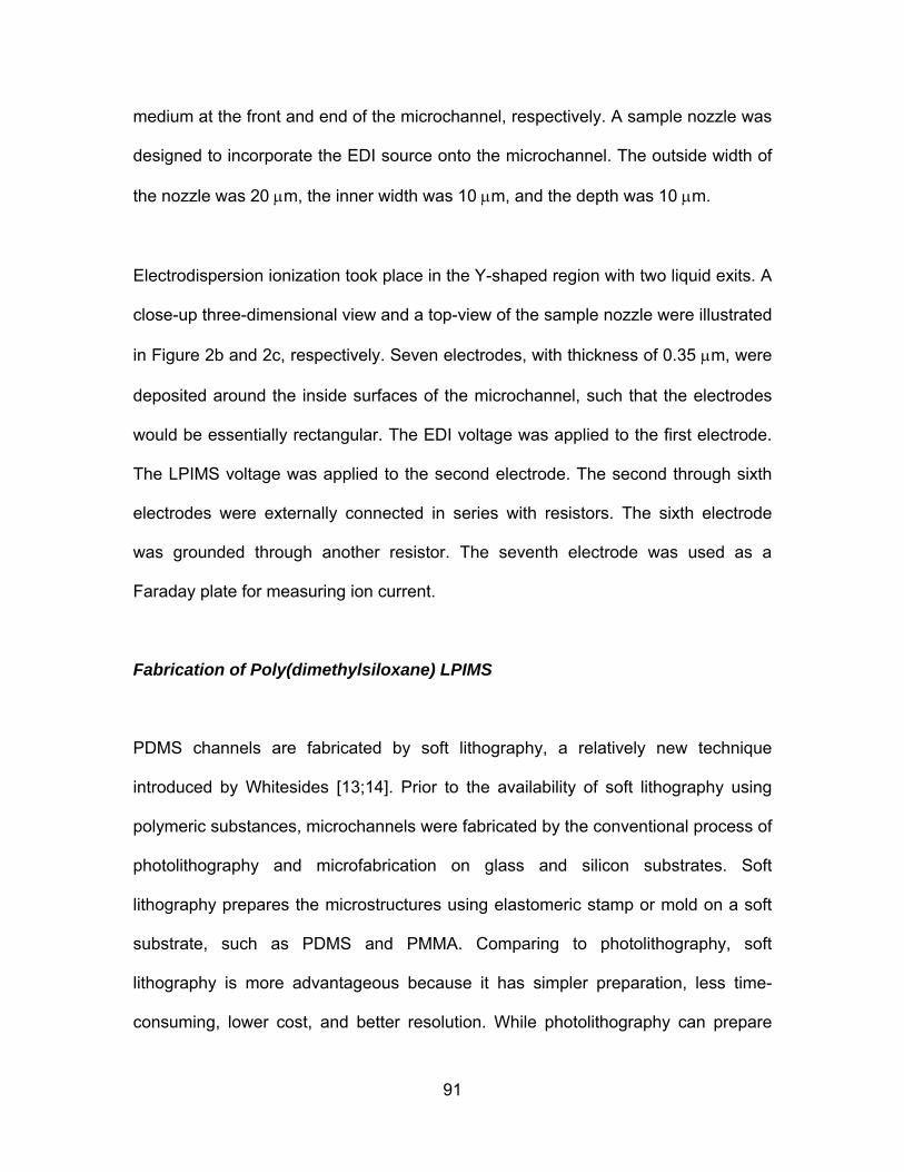
91

medium at the front and end of the microchannel, respectively. A sample nozzle was

designed to incorporate the EDI source onto the microchannel. The outside width of

the nozzle was 20 μm, the inner width was 10 μm, and the depth was 10 μm.

Electrodispersion ionization took place in the Y-shaped region with two liquid exits. A

close-up three-dimensional view and a top-view of the sample nozzle were illustrated

in Figure 2b and 2c, respectively. Seven electrodes, with thickness of 0.35 μm, were

deposited around the inside surfaces of the microchannel, such that the electrodes

would be essentially rectangular. The EDI voltage was applied to the first electrode.

The LPIMS voltage was applied to the second electrode. The second through sixth

electrodes were externally connected in series with resistors. The sixth electrode

was grounded through another resistor. The seventh electrode was used as a

Faraday plate for measuring ion current.

Fabrication of Poly(dimethylsiloxane) LPIMS

PDMS channels are fabricated by soft lithography, a relatively new technique

introduced by Whitesides [13;14]. Prior to the availability of soft lithography using

polymeric substances, microchannels were fabricated by the conventional process of

photolithography and microfabrication on glass and silicon substrates. Soft

lithography prepares the microstructures using elastomeric stamp or mold on a soft

substrate, such as PDMS and PMMA. Comparing to photolithography, soft

lithography is more advantageous because it has simpler preparation, less time-

consuming, lower cost, and better resolution. While photolithography can prepare

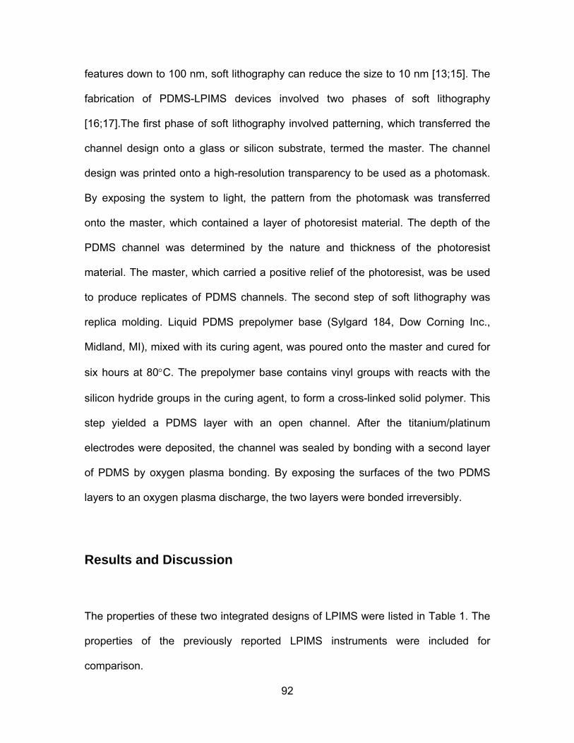
92

features down to 100 nm, soft lithography can reduce the size to 10 nm [13;15]. The

fabrication of PDMS-LPIMS devices involved two phases of soft lithography

[16;17].The first phase of soft lithography involved patterning, which transferred the

channel design onto a glass or silicon substrate, termed the master. The channel

design was printed onto a high-resolution transparency to be used as a photomask.

By exposing the system to light, the pattern from the photomask was transferred

onto the master, which contained a layer of photoresist material. The depth of the

PDMS channel was determined by the nature and thickness of the photoresist

material. The master, which carried a positive relief of the photoresist, was be used

to produce replicates of PDMS channels. The second step of soft lithography was

replica molding. Liquid PDMS prepolymer base (Sylgard 184, Dow Corning Inc.,

Midland, MI), mixed with its curing agent, was poured onto the master and cured for

six hours at 80°C. The prepolymer base contains vinyl groups with reacts with the

silicon hydride groups in the curing agent, to form a cross-linked solid polymer. This

step yielded a PDMS layer with an open channel. After the titanium/platinum

electrodes were deposited, the channel was sealed by bonding with a second layer

of PDMS by oxygen plasma bonding. By exposing the surfaces of the two PDMS

layers to an oxygen plasma discharge, the two layers were bonded irreversibly.

Results and Discussion

The properties of these two integrated designs of LPIMS were listed in Table 1. The

properties of the previously reported LPIMS instruments were included for

comparison.

93

A. Liquid Containment

i) Low Temperature Co-fired Ceramics LPIMS

The containment of the liquid medium within the LPIMS was achieved for both

LTCC-LPIMS and PDMS-LPIMS devices. There were several noteworthy

operational details. The end surfaces of the LTCC-LPIMS mobility tube was ground

smooth to ensure a tight seal between the Teflon end caps and the mobility tube.

The distance between the second and the third Teflon end caps was equal at all

points around the circumference of the mobility tube for proper alignment between

the external electrical connectors on the underside of the mobility tube and the pogo

pins in the third end cap. This alignment was also necessary for sealing the mobility

tube between the two end caps. The firing process had caused internal cracks, from

the center channel to an alignment pinhole, within one structure, which caused liquid

medium from the center channel to leak through the alignment pinhole. This was

resolved by sealing the alignment pins inside their pinholes with epoxy.

ii) Poly(dimethylsiloxane) LPIMS

The infusion of non-polar organic solvent into the PDMS microchannel with was

impeded by the nature of the PDMS surface. The surface of PDMS is hydrophobic

due to the methyl groups. During the oxygen plasma process, which was used to

bond two layers of PDMS, the methyl group on the PDMS surface is oxidized to

silanol groups [9] (Figure 3)[18]. The PDMS surface remained hydrophilic if it were in

contact with water, which was used to clean the microchannels following the

fabrication process. However, the oxidation of surface methyl groups is reversible in

94

air within 30 minutes [9], and the infusion difficulty was overcome by injecting air

through the microchannel for 30 minutes, prior to introduction of liquid medium. The

typical resistivity values between pairs of adjacent electrodes of an empty PDMS

microchannel were listed in Table 2. The resistance between adjacent pair of

electrodes was usually in the 1011 Ω range for a freshly prepared microchannel. After

rinsing the channel with air for 30 minutes, the surface of the microchannel returned

to being hydrophobic and the resistance between adjacent pair of electrodes was

normally in the 1012 Ω range.

B. Electrical Integrity


The LTCC mobility tube was made by stacking multiple layers of LTCC sheets with

printed conducting electrodes and resistance materials. Electrical integrity was

achieved by preventing misalignment. Two alignment holes were drilled at the same

position for each layer. Alignment pins were used to arrange the multiple layers in a

stacking position. The most significant disadvantage of the LTCC-LPIMS device was

the 20% variation in resistivity of the resistance material. This problem could be

solved by trimming the resistance material with laser after the firing process [7].

However, the laser trimming was not feasible for this LTCC device because the

resistance materials were embedded. The large variance in resistivity would severely

affect the homogeneity of the applied electric field, and thus lowering the resolving of

the instrument. Improvement in layer-to-layer resistivity reproducibility would be

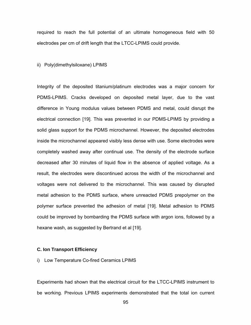
95

required to reach the full potential of an ultimate homogeneous field with 50

electrodes per cm of drift length that the LTCC-LPIMS could provide.


Integrity of the deposited titanium/platinum electrodes was a major concern for

PDMS-LPIMS. Cracks developed on deposited metal layer, due to the vast

difference in Young modulus values between PDMS and metal, could disrupt the

electrical connection [19]. This was prevented in our PDMS-LPIMS by providing a

solid glass support for the PDMS microchannel. However, the deposited electrodes

inside the microchannel appeared visibly less dense with use. Some electrodes were

completely washed away after continual use. The density of the electrode surface

decreased after 30 minutes of liquid flow in the absence of applied voltage. As a

result, the electrodes were discontinued across the width of the microchannel and

voltages were not delivered to the microchannel. This was caused by disrupted

metal adhesion to the PDMS surface, where unreacted PDMS prepolymer on the

polymer surface prevented the adhesion of metal [19]. Metal adhesion to PDMS

could be improved by bombarding the PDMS surface with argon ions, followed by a

hexane wash, as suggested by Bertrand et al [19].

C. Ion Transport Efficiency


Experiments had shown that the electrical circuit for the LTCC-LPIMS instrument to

be working. Previous LPIMS experiments demonstrated that the total ion current

96

between 1 and 2 nA was obtained from ionizing an aqueous sample at 0.5 μL/min

with an EDI voltage of 1000 V above the target screen, for a drift distance of 2 mm.

The LTCC-LPIMS had a drift length of 18.9 mm. The applied electric field of the drift

region was 586 V/cm. The sample was an aqueous solution of 10 μM basic fuchsin,

dissolved in methanol-water (90:10, vol/vol). The sample flow rate was 0.5 μL/min.

The drift liquid, benzene, had a flow rate of 100 μL/min, or a linear velocity of 0.015

cm/s. The linear velocity of basic fuchsin in benzene at 586V/cm was anticipated to

be 1 cm/s. Therefore, the counterflow of benzene should impede the migration of

basic fuchsin ions by only 1.5% and would not hamper ion detection.

The EDI current data was tabulated in Table 3. When the EDI voltage and the

LPIMS tube voltage were both zero, there was no current registered. When 2000V

was applied to the mobility tube, 0.127 nA was measured. This current originated

from the benzene background. When 2000V was applied to the EDI source, no

ionization should occur because the EDI voltage equaled that of the target screen.

There was no electric field between the EDI source and the LPIMS tube to induce

ionization. However, a higher current of 0.137 nA was measured. As the EDI voltage

increased, while maintaining the LPIMS voltage at 2000V, the total ion current also

increased. When the EDI voltage was 1000V above that of the target screen, 0.145

nA was measured, which was 0.018 nA above the background current of 0.127 nA.

A control test was run at the end of the experiment set, the target screen was

maintained at 2000V, but there was no applied EDI voltage. The current measured

for the control test was 0.158 nA, which was the highest current level detected for

97

the experiment set. This indicated that the background current level rose with

experimental time. The current was possibly arisen from water droplets

contamination and not originating from EDI. The results for ion transport efficiency

were inconclusive. Further testing will be necessary.


To evaluate ion transport in PDMS-LPIMS microchannel, total ion current was

measured with successive electrodes being used as the Faraday plate. The liquid

medium, benzene, was flowing at a rate of 5 μL/min. The EDI voltage was applied to

electrode 1 and was set at 1500V above that of the electrode 2. The electric field of

the channel was set at +800V per electrode, except when the electrode 2 was used

as the Faraday plate. For example, when the total ion current was being measured

at the electrode 3, +800V was applied to the electrode 2; and when the total ion

current was being measured at the electrode 7, +4000V, +3200V, +2400V, +1600V,

and +800V were applied to the electrode 2, 3, 4, 5, and 6, respectively. Using

electrode 2 as the Faraday plate was equivalent to measuring ion detection right

after ionization. Measuring current at electrode 3 and beyond was equivalent to

allowing the electrodispersed ion to travel along a length of ion mobility tube prior to

ion detection. Therefore, effectiveness of ion transport can be determined by

expressing the ion current detected as a fraction of the total electrodispersed current

detected at the electrode 2.

98

The first set of experiments used benzene as the sample, and methanol-water

(90:10, vol/vol) was used in the second set of experiments. The sample flow rate

was 0.5 μL/min. Figure 4 showed the total ion current measured at successive

electrodes along the PDMS channel in benzene with the two samples. The data

showed that EDI signal of methanol-water was substantially greater than that of

benzene. The EDI signal of methanol-water decreased with the increasing distance

traveled. The ion transport efficiency declined to 32% of total electrodispersed ion

current at electrode 3 and 0.45% at electrode 4. The results showed that the EDI

signal could not be detected beyond the electrode 4, or a distance of 4 mm. The

rapid reduction in ion transport efficiency with increasing migration distance could be

hindered by the electrode design. The current electrodes were 1 mm wide and the

electrodes spacing was also 1 mm. For the length of 10 mm from electrode 2 to

electrode 7, there were 5 mm of zero-field region where the main ion movement was

by diffusion. Future designs of PDMS-LPIMS should utilize narrower electrode

widths.

Acknowledgements



99

References


2. H. H. Hill, Jr. and M. Tam. Ion Mobility Spectrometry Method and Apparatus. US Patent 7,071,465. 2006.


4. M. Tam and Jr. H. H. Hill, Electrodispersion Ionization in Liquids, Submitted (2006).

5. J. P. Carrico, D. W. Sickenberger, G. E. Spangler and K. N. Vora, Simple Electrode Design for Ion Mobility Spectrometer, J. Phys. E: Sci. Instrum. 16, pp. 1058-1062 (1983).

6. G. E. Spangler, K. N. Vora and J. P. Carrico, Miniature Ion Mobility Spectrometer Cell, J. Phys. E: Sci. Instrum. 19, pp. 191-198 (1986).


8. P. A. Auroux, D. Iossifidis, D. R. Reyes and A. Manz, Micro Total Analysis Systems. 2. Analytical Standard Operations and Applications, Analytical Chemistry 74, pp. 2637-2652 (2002).

9. S. K. Sia and G. M. Whitesides, Microfluidic Devices Fabricated in Poly(dimethylsiloxane) for Biological Studies, Electrophoresis 24, pp. 3563-3576 (2003).

10. C. S. Effenhauser, G. J. M. Bruin, A. Paulus and M. Ehrat, Integrated Capillary Electrophoresis on Flexible Silicone Microdevices: Analysis of DNA Restriction Fragments and Detection of Single DNA Molecules on Microchips, Analytical Chemistry 69, pp. 3451-3457 (1997).

11. K. Huikko, P. Östman, K. Grigoras, S. Tuomikoski, V. -M. Tianen, A. Soininen, K. Puolanne, A. Manz, S. Franssila, R. Kostiainen and T. Kotiaho, Poly(dimethylsiloxane) Electrospray Devices Fabricated with Diamond-like Carbon-Poly(dimethylsiloxane) Coated SU-8 Masters, Lab Chip 3, pp. 67-72 (2003).

12. Donald Gene Plumlee, Fabrication of a Miniature Ion Mobility Spectrometry in

100

Low Temperature Co-fired Ceramics, Boise State University, Boise, Idaho (2003).

13. Y. Xia and G. M. Whitesides, Soft Lithography, Angewandte Chemie International Edition 37, pp. 550-575 (1998).

14. J. C. McDonald and G. M. Whitesides, Poly(dimethylsiloxane) as a Material for Fabricating Microfluidic Devices, Accounts of Chemical Research 35, pp. 491-499 (2002).

15. W. W. Y. Chow, K. F. Lei, G. Shi, W. J. Li and Q. Huang, Microfluidic Channel Fabrication by PDMS-Interface Bonding, Smart Materials and Structures 15, p. S112-S116 (2006).

16. H. Cui, K. Horiuchi, P. Dutta and C. F. Ivory, Isoelectric Focusing in a Poly(dimethylsiloxane) Microfluidic Chip, Analytical Chemistry 77, pp. 1303-1309 (2005).

17. N. H. Al Mamum, Fabrication of a Microchip Device for Liquid Phase Ion Mobility Spectrometry, Washington State University, Pullman, WA (2006).

18. D. C. Duffy, J. C. McDonald, O. J. A. Schueller and G. M. Whitesides, Rapid Prototyping of Microfluidic Systems in Poly(dimethylsiloxane), Analytical Chemistry 70, pp. 4974-4984 (1998).

19. A. Delcorte, S. Befany, C. Poleunis, M. Troosters and P. Bertrand, Improvement of Metal Adhesion to Silicone Films: a TOF-SIMS Study. In Adhesion Aspects of Thin Films (Edited by K. L. Mittal), VSP, The Netherlands (2005).

101

Table 1: Properties and dimensions of the previously reported and integrated

LPIMS devices.

Previously Reported Devices

Integrated Devices

Teflon

Resistive

Glass

LTCC

PDMS

Housing Material:

Teflon

Pyrex

LTCC

PDMS

Channel Properties:

Shape Cylindrical Cylindrical Cylindrical Rectangular Cross Section 4.76 mm i.d. 4.1 mm i.d. 3.8 mm i.d. 1.0 mm (w)

0.4 mm (h) Total Length (mm) 20.0 14.5 18.1 10.0 Drift Length (mm)

13.3 5.0 10.4 10.0

Resistors:

External

Surface

Embedded

External

Number of electrodes:

16

Continuous

65

6

Insulator: Material Teflon n/a LTCC PDMS

Resistivity (ohm-cm) 1018 n/a 1014 1013

Dielectric Strength (kV/mm)

60 n/a 20 21

Sample Introduction:

Fused silica

capillary

Fused silica

capillary

Fused silica

capillary

Sample nozzle

incorporated into main channel

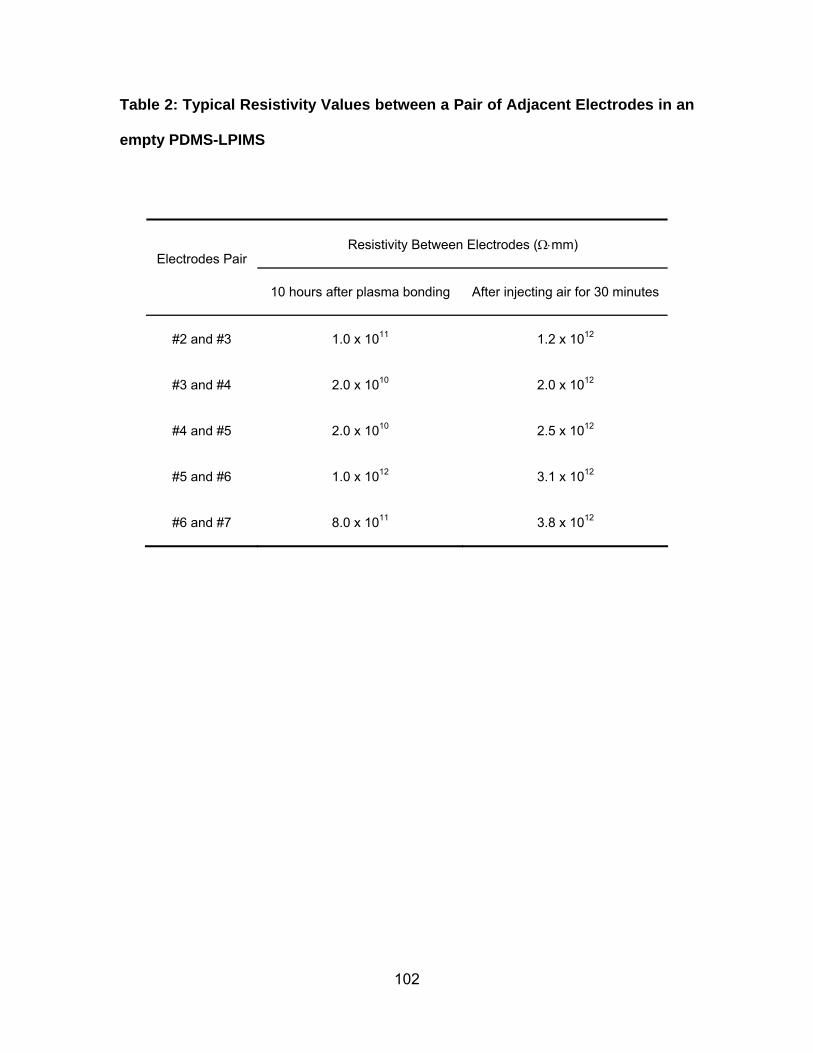
102

Table 2: Typical Resistivity Values between a Pair of Adjacent Electrodes in an

empty PDMS-LPIMS

Resistivity Between Electrodes (Ω⋅mm)

Electrodes Pair

10 hours after plasma bonding

After injecting air for 30 minutes

#2 and #3

1.0 x 1011

1.2 x 1012

#3 and #4

2.0 x 1010

2.0 x 1012

#4 and #5

2.0 x 1010

2.5 x 1012

#5 and #6

1.0 x 1012

3.1 x 1012

#6 and #7

8.0 x 1011

3.8 x 1012

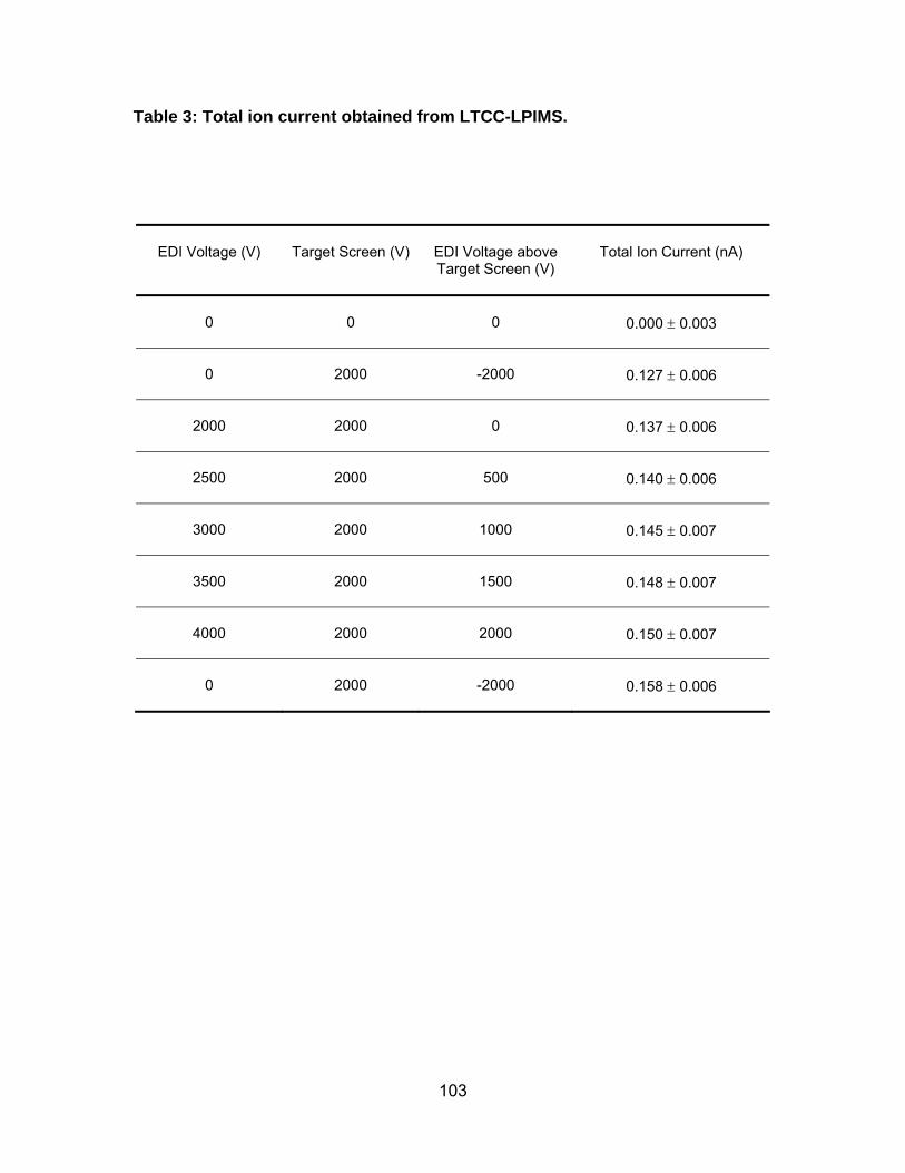
103

Table 3: Total ion current obtained from LTCC-LPIMS.

EDI Voltage (V)

Target Screen (V)

EDI Voltage above Target Screen (V)

Total Ion Current (nA)

0

0

0

0.000 ± 0.003

0

2000

-2000

0.127 ± 0.006

2000

2000

0

0.137 ± 0.006

2500

2000

500

0.140 ± 0.006

3000

2000

1000

0.145 ± 0.007

3500

2000

1500

0.148 ± 0.007

4000

2000

2000

0.150 ± 0.007

0

2000

-2000

0.158 ± 0.006

104

Figure Captions

Figure 1: Schematic of the LTCC-LPIMS (A) with its sealing Teflon end caps (B),

external electrical connections (C), liquid medium entry (D) and exit (E). The three

pieces of Teflon end caps were tightened with three screws (F), and sealed with two

pieces of o-rings (G) and a membrane (H) that fitted into the counter bore of the end

caps.

Figure 2: (a) Top-view schematic of the third generation of PDMS-LPIMS prototype.

The PDMS channel was 1000 μm wide, 400 μm deep and 1 cm long. (b) Close-up

three-dimensional view and (c) top-view of the sample nozzle. The outside width of

the nozzle was 50 μm, the inner width was 10 μm, and the depth was 10 μm.

Figure 3: The surface methyl groups of poly(dimethylsiloxane) are oxidized to

hydroxyl group by oxygen plasma. The oxidation reaction is reversible in air within

30 minutes.

Figure 4: Plot of total ion current being measured at successive electrodes along the

PDMS channel in benzene. The sample used were benzene ( ) and methanol-water

(90:10, vol/vol) ( ).

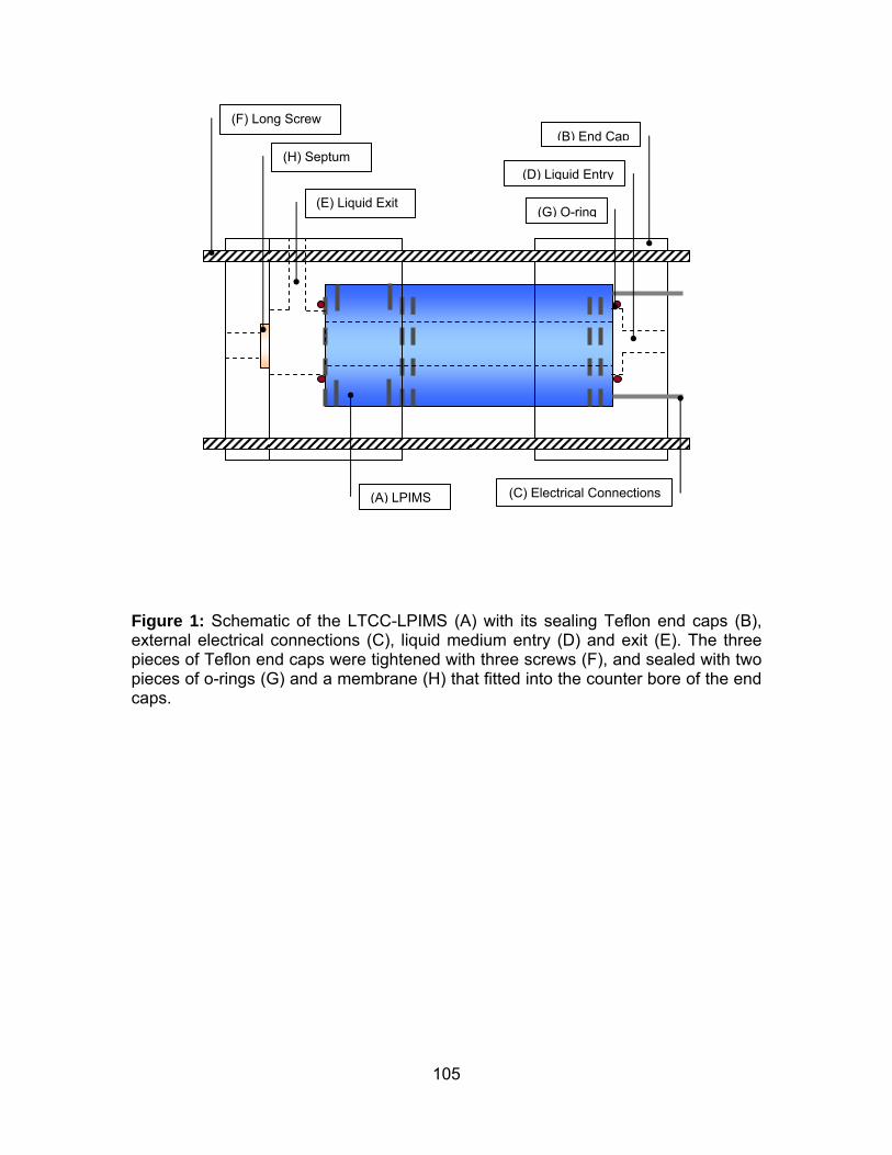
105

Figure 1: Schematic of the LTCC-LPIMS (A) with its sealing Teflon end caps (B), external electrical connections (C), liquid medium entry (D) and exit (E). The three pieces of Teflon end caps were tightened with three screws (F), and sealed with two pieces of o-rings (G) and a membrane (H) that fitted into the counter bore of the end caps.

(B) End Cap

(C) Electrical Connections

(F) Long Screw

(H) Septum (D) Liquid Entry

(A) LPIMS

(E) Liquid Exit (G) O-ring

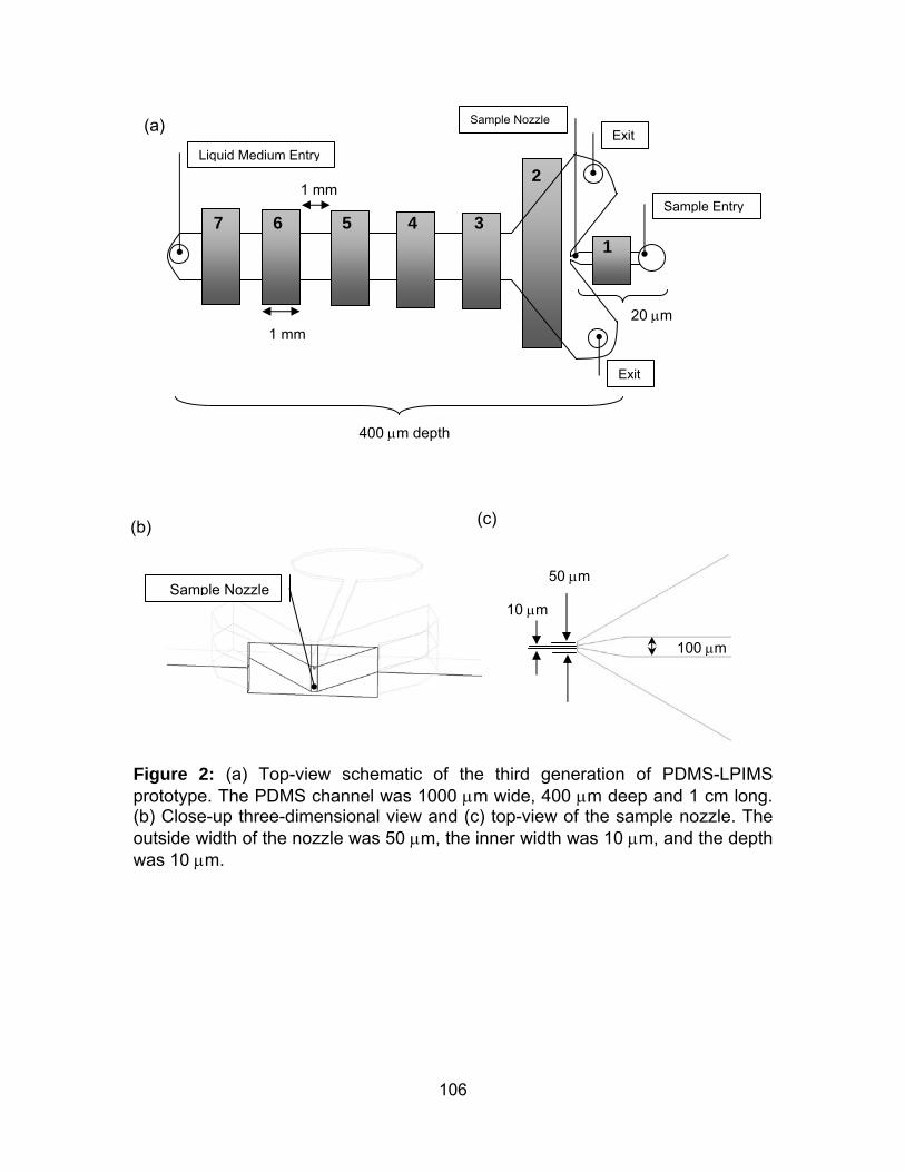
106

Figure 2: (a) Top-view schematic of the third generation of PDMS-LPIMS prototype. The PDMS channel was 1000 μm wide, 400 μm deep and 1 cm long. (b) Close-up three-dimensional view and (c) top-view of the sample nozzle. The outside width of the nozzle was 50 μm, the inner width was 10 μm, and the depth was 10 μm.

(a) Sample Nozzle

1

2

3 4 5 6 7

1 mm

1 mm 20 μm

400 μm depth

Sample Entry

Liquid Medium Entry

Exit

Exit

(b) (c)

10 μm

100 μm

Sample Nozzle 50 μm

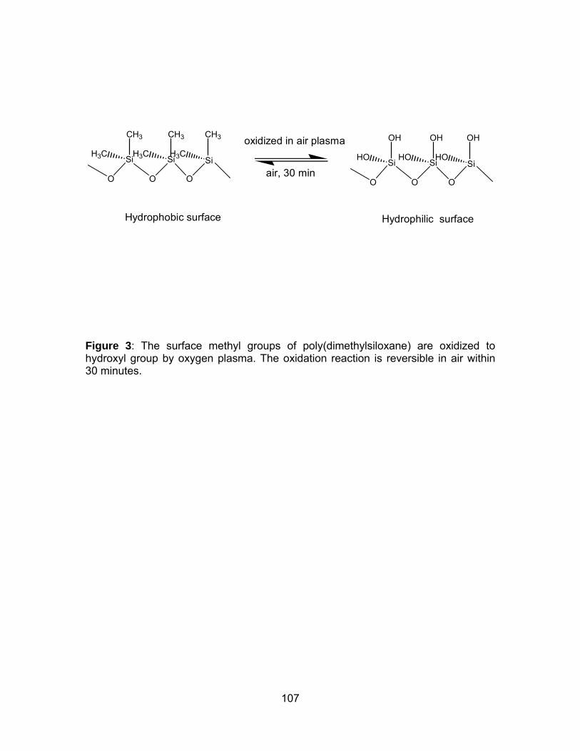
107

Si

CH3

OO

H3C Si

O

CH3

H3CSi

CH3

H3CSi

OH

OO

HO Si

O

OH

HOSi

OH

HO

air, 30 min

oxidized in air plasma

Hydrophobic surface Hydrophilic surface

Figure 3: The surface methyl groups of poly(dimethylsiloxane) are oxidized to hydroxyl group by oxygen plasma. The oxidation reaction is reversible in air within 30 minutes.

108

2.5

2.0

1.5

1.0

0.5

0.0

Tota

l Ion

Cur

rent

(nA)

654321

Electrode Number Used as Faraday Plate

Sample = BenzeneSample = Methanol-Water (9:1, v/v)

Figure 4: Plot of total ion current being measured at successive electrodes along the PDMS channel in benzene. The sample used were benzene ( ) and methanol-water (90:10, vol/vol) ( ).

109

Chapter Five

Evaluation of Pulsed Electrodispersion Ionization

Source for Liquid Phase Ion Mobility

Spectrometry

Abstract

Pulsed electrodispersion ionization source was developed and evaluated for liquid

phase ion mobility spectrometry in liquid hexane. The pulsed electrodispersion was

achieved by alternating the voltage applied to the ionization source, between a

voltage sufficient to induce electrodispersion and a lower voltage. A miniaturized

resistive glass liquid phase mobility spectrometer of 5 mm length was used. The use

of a pulsed ionization eliminated the need for an ion shutter. Liquid phase ion

mobility spectra of methanol-water solvent, tetramethylammonium,

tetrabutylammonium, and bradykinin demonstrated the capability of pulsed

electrodispersion ionization as a multipurpose ionization source for liquid phase ion

mobility spectrometry. This study presented pulsed electrodispersion ionization as a

multipurpose ionization source for generating liquid phase ions. Three important

instrumental processes were merged into a single source: sample introduction,

sample ionization, and pulsed ion injection.

110

Introduction

Liquid phase ion mobility spectrometry (LPIMS) is a newly developed analytical

separation technique [1-3]. The separation is based upon the difference in mobilities

of ions traveling through a non-electrolytic liquid medium under the influence of an

externally established electric field. Ionization in LPIMS was achieved by

electrodispersion ionization (EDI) [4], which was designed to deliver aqueous ions

into non-aqueous liquid medium. LPIMS is a time-of-flight analyzer that detects ion

signal as a function of the analyte arrival time. Because EDI is a continuous

ionization source, an ion shutter was used to introduce short pulses of ions into

LPIMS [5]. It is anticipated that a pulsed ionization source would be appropriate for

LPIMS.

Other time-of-flight analyzer, time-of-flight mass spectrometer (TOF-MS) and gas-

phase ion mobility spectrometer (IMS), interface well with pulsed ionization sources.

Pulsed glow discharge-TOF-MS is used to provide rapid elemental and molecular

analyses through its sequential “hard” and “soft” ionization processes [6-11]. Matrix-

assisted laser desorption ionization is a widely used ionization source for TOF-MS,

performing routine mass measurements of peptides and proteins [12-14] and

enabling analysis of biomolecules and synthetic polymers up to 350 kDa with sub

picomole sensitivities [15-17].

Early works of gas-phase IMS were conducted with pulsed ionization sources, such

as electron-impact [18-23], Townsend discharge [24-26], thermionic emitter [19;27],

111

and spark discharge sources [28]. These ion mobility spectrometers contained no

physical ion shutters because the ionization pulses were short, in comparison to the

drift times. The pulsing of the ionization source doubled as the gating mechanism.

Bradbury-Nielsen shutter [29] and Tyndall shutter [30] were implemented into ion

mobility spectrometers to provide more precise timing of ions [31-35]. With the

introduction of ion shutters, continuous ionization sources, such as radioactive

ionization and electrospray ionization, are made compatible with IMS. Radioactive

ionization sources (63Nickel, 241Americium, and Tritium) are frequently employed in

portable and handheld IMS instruments because they require neither power supply

nor maintenance. Radioactive ionization-IMS has been used for detecting a diversity

of compounds, from atmospheric [36;37] and environmental [38-42] pollutants,

explosives [43-45], drugs [46-49], chemical warfare agent simulants [50;51], to

derivatized whole cell bacteria [52]. Electrospray ionization-IMS was introduced in

the late 1980s [53] that had become invaluable in the research of proteomics [54-

60], glycomics [61-63], and metabolomics [64]. In addition to these popular

continuous ionization sources, there are current reports in exploring pulsed

ionization sources for IMS. Pulsed corona discharge ionization and distributed

plasma ionization were developed as alternative non-radioactive ionization sources

[65-70]. MALDI was used as a interchangeable replacement of EDI to make use of

its capability to form primarily singly charged ions and its ability to ionize bio- and

synthetic polymers [71-76].

EDI is the liquid phase analogue of electrospray ionization (ESI). Like ESI, which

was recently developed in pulsation mode with mass spectrometry [77-80], EDI can

operate in continuous and pulsing modes. The pulsing of EDI is controlled by

112

adjusting the applied EDI voltage relative to the sample flow rate [4]. The goal of this

study was to demonstrate the merge of three important instrumental processes:

sample introduction, sample ionization, and ion gating, in pulsed EDI for miniaturized

liquid phase ion mobility spectrometry.


Instrumentation

The pulsed EDI-LPIMS system consisted of a pulsed electrodispersion ionization

source and a liquid phase ion mobility spectrometer (Figure 1). The pulsed EDI

source comprised of a standard electrodispersion ionization source [4] and a pulsed

voltage circuit. Aqueous sample was introduced by a syringe that was connected

through a grounded metal union to a fused silica capillary. EDI voltage was applied

to a second metal union. A micro-elbow junction allowed for a 90° bend of the fused

silica capillary. The pulsed voltage circuit contained four 2.5 MΩ resistors in series

and was controlled by a Double Pole Single Throw (DPST) two-way switch,

constructed by Technical Services of Washington State University. The EDI voltage

was alternated between an upper voltage and a lower voltage. The upper voltage

was sufficient to induce electrodispersion ionization, which was 2200V above the

voltage of the spectrometer. There was no ionization at the lower voltage, which was

half the value of the upper voltage. The pulsed voltage circuit was capable of

switching a maximum voltage of 10 kV. The pulse width and frequency was

synchronized with a LabView (National Instruments, Austin, TX)-based data

113

acquisition program [81]. At the beginning of each mobility experiment, a 5-V signal

was sent by the data acquisition program to the two-way switch, opening the first

two-way switch and closing the second two-way switch for the duration of the pulse

width, 0.05 s, at a frequency of 0.1 Hz. At the end of the 0.05 s pulse, the first two-

way switch closed and the second two-way switch opened.

The liquid phase ion mobility spectrometer consisted of a resistive glass tube (Burle

Electro-Optics Inc., Sturbridge MA) and a Faraday plate (Figure 1). The resistive

glass tube had a 4.1-mm i.d., 5-mm length, and a total inner surface resistance of 10

MΩ. There were electrodes attached to either ends of the spectrometer. +500 V the

was applied to the front electrode of the spectrometer. The spectrometer was

grounded through a 430 kΩ resistor at the end electrode. The Faraday plate was

located 2 mm behind the spectrometer. The current signal was amplified at 109

volts/ampere by a Keithley 427 model (Keithley Instruments, Cleveland, OH) and

acquired by the data acquisition program.

Materials and Reagents

The liquid medium, through which ions drifted, was hexane (J. T. Baker, Phillipsburg,

NJ). Tetraalkylammonium salts and bradykinin (Sigma-Aldrich, St. Louis, MO) in

micro-molar concentrations were used as the sample analytes. The samples were

prepared in methanol-water (90:10, vol/vol) with HPLC grade methanol (J. T. Baker,

Phillipsburg, NJ) and 18.1 MΩ water. Tetramethylammonium bromide and

tetrabutylammonium bromide were individually dissolved as 10 mM solutions and

114

further diluted to 10 μM and 100 μM. Bradykinin was prepared from bradykinin

acetate as 10 mM solutions and diluted to 100 μM. The solvent blank was methanol-

water (90:10, vol/vol).

Calculations

Liquid phase ion mobility (μ) was calculated as the ratio of ion velocity (v) to the

applied electric field (E). In terms of the spectrometer length (L) and the mobility time

(t), the liquid phase ion mobility was expressed as:

Lμ =E t⋅

(1)

Because the liquid phase ion mobility spectrometry was miniaturized, with a length of

5 mm (L1), the distance between the end of the resistive glass mobility spectrometer

and the Faraday plate (L2) became significant. It would be necessary to take into

consideration the electric field between the end of the spectrometer and the Faraday

plate for the mobility calculation. The distance of L2 was 2 mm. When a voltage of

+507 V was applied to the front electrode of the spectrometer, the end electrode had

a voltage of +18 V. Therefore, the electric field across L1 was +978 V/cm (E1) and

the electric field across L2 was +90V/cm (E2). Therefore, the mobility value was more

accurately represented as:

1 2

1 2

L L 1μ = +E E t⎛ ⎞

⋅⎜ ⎟⎝ ⎠

(2)

115

The expected mobility values of ions in hexane (μ in hexane) were estimated by

adjusting the literature mobility values of ions in water (μ in water) for the viscosity

difference between the two liquid medium.

in hexanewater

in waterhexane

ημ = μ ×

η (3)

Water has a viscosity of 0.89 cP, while the less viscous hexane has a viscosity of

0.326 cP [82]. Consequently, analytes are expected to have 2.7 times faster

mobilities in hexane than in water, as the mobility of ions is inversely proportional to

the viscosity of the liquid medium [83].


LPIMS Spectra of Solvent Blank

Liquid phase ion mobility spectra of the methanol-water solvent blank were obtained

using pulsed electrodispersion ionization for sample introduction, sample ionization,

and ion gating. 179 spectra were collected consecutively over 30 minutes at 10-s

intervals. An EDI voltage of +2700 V was applied for a pulse width of 0.05 s.

The solvent peaks shifted to longer mobility time over the course of the experiment.

The first 8.5 minutes of the data (51 averages), the last 2.5 minutes of data (15

averages), and the entire 30 minutes of data (179 averages) were compared (Figure

116

2). There were two solvent peaks, at 0.49 s and 0.54 s, observed in the averaged

spectrum for the first 8.5 minutes of the experiment (Figure 2a). The solvent peaks

had shifted to 0.62 s, 0.67 s, 0.73 s, and 0.80 s in the averaged spectrum in the last

2.5 minutes of the experiment (Figure 2b). The solvent peaks were assumed to be

solvated proton ions. The fact that the mobility time of the solvent peaks increased

with experimental duration suggested that the solvent ions were surrounded by an

increasing amount of solvation molecules. Conventional gas phase ion mobility

spectrometry has a unidirectional counter flow of drift gas that keep the drift region

clean by continuously sweeping out neutral molecules [84]. Because the liquid

hexane medium was stationary in this study, any uncharged solvent molecules

would remain inside the spectrometer. Subsequent ion-molecule reactions, between

ionized and uncharged solvent molecules, produced ions of increasing sizes and

longer drift times.

The three-dimensional plot of current intensity, mobility time, and consecutive

spectrum number (Figure 3) revealed that two populations of ions were present: a

major group of ions with a drift time of 0.51 s (A in Figure 3) and a minor group of

ions with drift times between 1 s and 2 s (B in Figure 3). The minor group of ions,

also observed in Figure 2c as a broad peak, was presumably larger cluster ions of

the solvent.

Figure 3 showed that the solvent peaks shifted progressively from 0.51 ± 0.05 s at

the start of the experiment, to 0.71 ± 0.06 s towards the end of the experiment. The

mobility value of the solvent ions, calculated with equation 2, had decreased from

117

(5.4 ± 0.5) x 10-3 cm2/V⋅s to (3.8 ± 0.3) x 10-3 cm2/V⋅s. The estimated mobility value

of proton in hexane, was calculated by adjusting the literature mobility value of

proton in water, (3.623 x 10-3 cm2/V⋅s) [85], for the viscosity difference (equation 3).

The estimated mobility value of proton in hexane was 9.9 x 10-3 cm2/V⋅s. However,

migration of proton in water involves a transfer process of proton among water

molecules through forming and disrupting hydrogen bonds. This mechanism of

proton migration, first proposed by Grotthuss [86] in 1806, is continually being

studied and modeled [87-89]. The Grotthuss mechanism was assumed to have

negligible effect in the liquid medium used in this experiment, as there are no

hydrogen bonds formed between the protons and the non-polar hexane. Therefore,

the migration of proton in hexane involves the actual movement of proton molecules

through hexane. The mobilities of solvated proton ions in hexane are therefore

expected to be slower than the estimated mobility of 9.9 x 10-3 cm2/V⋅s in the

absence of proton migration by Grotthus mechanism. The experimental mobility

value of 5.4 x 10-3 cm2/V⋅s for the solvent ions in hexane was indeed slower than the

estimated mobility of proton in hexane by 1.8 times.

LPIMS Spectra of Analytes

Pulsed EDI-LPIMS of tetramethylammonium bromide, tetrabutylammonium bromide,

and bradykinin were conducted in hexane in the positive mode. The samples were

dissolved in the solvent blank of methanol-water (90:10, vol/vol) at a concentration of

100 μM. The sample flow rates were 0.1 μL/min. An EDI voltage of +2650 V was

applied for a pulse width of 0.05 s.

118

The EDI-LPIMS spectra of tetramethylammonium, tetrabutylammonium ions, and

bradykinin were shown in Figure 4a – 4c. All the analyte spectra showed a sharp

and intense peak. Both tetraalkylammonium spectra featured a 0.28 s peak and the

bradykinin spectrum had a 0.19 s peak. It was assumed that the 0.19 s and the 0.28

s peaks were not an analyte peak since it had a faster mobility time than the solvent

ions. Tetramethylammonium spectrum had a unique peak at 0.76 s, with a

corresponding mobility value of 3.6 x 10-3 cm2/V⋅s; while tetrabutylammonium

spectrum had a characteristic peak at a slower mobility time of 0.89 s, with a mobility

value of 3.1 x 10-3 cm2/V⋅s. The bradykinin spectrum had overlapping peaks between

0.6 s and 1.7 s, with the two most intense peaks at 0.67 s and 1.18 s. The 0.67 s

peak in the bradykinin spectrum was most likely solvent ions, because its mobility

value of 4.1 x 10-3 cm2/V⋅s was in close proximity to that of the solvent ions.

The experimental mobility values of tetramethylammonium, tetrabutylammonium,

and bradykinin were compared with the literature mobility values in water and the

estimated mobility values in hexane (Table 1). The mobility value of bradykinin in

water was not available in literature and thus, the mobility value for a fluorescein

isothiocyanate (FITC)-labeled bradykinin was provided instead. The FITC label

increased the mass of bradykinin from 1060 Da to 1436 Da [90]. While the mobility

value of the solvent ions were slower than that expected in hexane, due to the

absence of Grotthus mechanism in non-polar hexane, the three analytes all had

faster mobilities than anticipated. Tetramethylammonium, with its mobility value of

3.6 x 10-3 cm2/V⋅s, was 2.8 times faster than its estimated mobility value in hexane;

tetrabutylammonium, with its mobility value of 3.6 x 10-3 cm2/V⋅s, was 5.6 times

119

faster; and bradykinin, with its mobility value of 2.3 x 10-3 cm2/V⋅s, was 6 times

faster. Ions in water are surrounded by a shell of solvation sphere due to the ion-

dipole interaction with water molecules [85]. Singh et al previously reported that, in

aqueous solutions of acetonitrile, the solvation sphere surrounding copper ions

consisted of acetonitrile molecules [91]. The replacement of solvation molecules,

from water to acetonitrile molecules, increased the hydrodynamic radius of the

copper ions. The mobility of copper ions was, therefore, slower in the aqueous

acetonitrile solution, compared with its mobility in water. Based on the same line of

reasoning, ions in hexane would not have a shell of solvation sphere due to the lack

of ion-dipole interaction between the ions and the non-polar hexane. As a result,

mobility of ions in hexane was faster than predicted.

Conclusions

Electrodispersion ionization is a liquid phase ionization source capable of generating

ions in short pulses. Pulsed electrodispersion ionization source is useful for pulsed

injection of aqueous ions in liquid phases. This is useful for liquid phase ion mobility

spectrometry, especially in a miniaturized instrument. A pulsed ionization source

eliminates the need for a physical ion shutter, thus simplifying the manufacturing

process. A pulsed ionization source also reduces sample consumption. The results

suggest that a counterflow of liquid medium will be useful in removing uncharged

molecule in the liquid phase ion mobility spectrometer.

120

Acknowledgements



121

References

1. H. H. Hill, Jr. and M. Tam. Ion Mobility Spectrometry Method and Apparatus. US Patent 7,071,465. July 4, 2006.



4. M. Tam and H. H. Hill, Jr. Electrodispersion Ionization in Liquids, Submitted (2006).

5. M. Tam and H. H. Hill, Jr. Liquid Phase Ion Mobility Spectrometry, Manuscript in Preparation (2006).

6. W. Hang, W. O. Walden and W. W. Harrison, Microsecond Pulsed Glow Discharge as an Analytical Spectroscopic Source, Analytical Chemistry 68, pp. 1148-1152 (1996).

7. R. E. Steiner, C. L. Lewis and V. Majidi, Consideration of a Millisecond Pulsed Glow Discharge Time-of-Flight Mass Spectrometer for Concurrent Elemental and Molecular Analysis, Journal of Analytical Atomic Spectrometry 14, pp. 1537-1541 (1999).

8. D. Fliefel, K. Fuhrer, M.Gonin and D. Gunther, Evaluation of a Pulsed Glow Discharge Time-of-Flight Mass Spectrometer as a Detector for Gas Chromatography and the Influence of the Glow Discharge Source Parameters on the Information Volume in Chemical Speciation Analysis, Analytical and Bioanalytical Chemistry 386, pp. 169-179 (2006).

9. R. E. Steiner, C. L. Lewis and F. L. King, Time-of-Flight Mass Spectrometry with a Pulsed Glow Discharge Ionization Source, Analytical Chemistry 69, pp. 1715-1721 (1997).

10. L. Li, C. M. Barshick, J. T. Millay, A. V. Welty and F. L. King, Determination of Bromine in Flame-Retardant Plastics Using Pulsed Glow Discharge Mass Spectrometry, Analytical Chemistry 75, pp. 3953-3961 (2003).

11. L. Li, J. T. Millay, J. P. Turner and F. L. King, Millisecond Pulsed Radio Frequency Glow Discharge Time of Flight Mass Spectrometry: Temporal and Spatial Variations in Molecular Energetics, Journal of the American Society for Mass Spectrometry 15, pp. 87-102 (2004).

122

12. M. Mann, R. C. Hendrickson and A. Pandey, Analysis of Proteins and Proteomes by Mass Spectrometry, Annual Review of Biochemistry 70, pp. 437-473 (2001).

13. W. Pusch and M. Kostrzewa, Application of MALDI-TOF Mass Spectrometry in Screening and Diagnositc Research, Current Pharmaceutical Design 11, pp. 2577-2591 (2005).

14. B. Spengler and R. J. Cotter, Ultraviolet-Laser Desorption Ionization Mass-Spectrometry of Proteins above 100000 Daltons by Pulsed Ion Extraction Time-of-Flight Analysis, Analytical Chemistry 62, pp. 793-796 (1990).

15. R. Kaufmann, Matrix-Assisted Laser Desorption Ionization (MALDI) Mass Spectrometry: a Novel Analytical Tool in Molecular Biology and Biotechnology, Journal of Biotechnology 41, pp. 155-175 (1995).

16. H. J. Rader and W. Schrepp, MALDI-TOF Mass Spectrometry in the Analysis of Synthetic Polymers, Acta Polymerica 49, pp. 272-293 (1998).

17. S. E. M. Moore, A. R. Hemsley, A. N. French, E. Dudley and R. P. Newton, New Insights from MALDI-TOF MS, NMR, and GC-MS: Mass Spectrometry Techniques Applied to Palynology, Protoplasma 228, pp. 151-157 (2006).

18. D. L. Albritton, T. M. Miller, D. W. Martin and E. W. McDaniel, Mobilities of Mass-Identified H3

+ and H+ Ions in Hydrogen, Physical Review 171, pp. 94-102 (1968).

19. T. M. Miller, J. T. Moseley, D. W. Martin and E. W. McDaniel, Reactions of H+ in H2 and D+ in D2; Mobilities of Hydrogen and Alkali Ions in H2 and D2 Gases, Physical Review 173, pp. 115-123 (1968).

20. J. T. Moseley, R. M. Snuggs, D. W. Martin and E. W. McDaniel, Mobilities, Diffusion Coefficients, and Reaction Rates of Mass-Identified Nitrogen Ions in Nitrogen, Physical Review 178, pp. 240-248 (1969).

21. J. Heimerl, R. Johnsen and M. A. Biondi, Ion-Molecule Reactions, He+ + O2 and He+ + N2, at Thermal Energies and Above, Journal of Chemical Physics 51, pp. 5041-5048 (1969).

22. H. L. B. a. M. A. B. R. Johnsen, Ion-Molecule Reactions Involving N2+, N+, O2+,

and O+ Ions from 300K to ~1eV, Journal of Chemical Physics 52, pp. 5080-5084 (1970).

23. R. M. S. D. W. M. a. E. W. M. J. T. Moseley, Longitudinal and Transverse Diffusion Coefficients of Mass-Identified N+ and N2

+ Ions in Nitrogen, Physical Review Letters 21, pp. 873-875 (1968).

24. J. A. Hornbeck, Microsecond Transient Currents in the Pulsed Townsend Discharge, Physical Review 58, pp. 374-379 (1951).

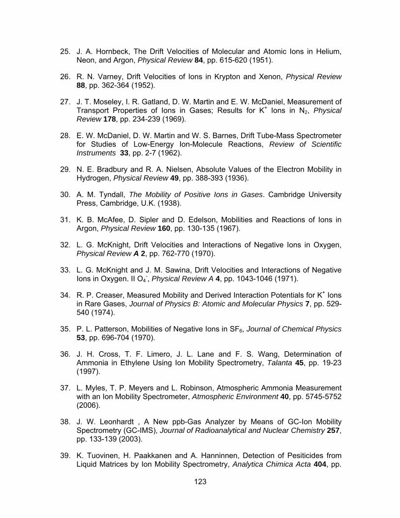
123

25. J. A. Hornbeck, The Drift Velocities of Molecular and Atomic Ions in Helium, Neon, and Argon, Physical Review 84, pp. 615-620 (1951).

26. R. N. Varney, Drift Velocities of Ions in Krypton and Xenon, Physical Review 88, pp. 362-364 (1952).

27. J. T. Moseley, I. R. Gatland, D. W. Martin and E. W. McDaniel, Measurement of Transport Properties of Ions in Gases; Results for K+ Ions in N2, Physical Review 178, pp. 234-239 (1969).

28. E. W. McDaniel, D. W. Martin and W. S. Barnes, Drift Tube-Mass Spectrometer for Studies of Low-Energy Ion-Molecule Reactions, Review of Scientific Instruments 33, pp. 2-7 (1962).

29. N. E. Bradbury and R. A. Nielsen, Absolute Values of the Electron Mobility in Hydrogen, Physical Review 49, pp. 388-393 (1936).

30. A. M. Tyndall, The Mobility of Positive Ions in Gases. Cambridge University Press, Cambridge, U.K. (1938).

31. K. B. McAfee, D. Sipler and D. Edelson, Mobilities and Reactions of Ions in Argon, Physical Review 160, pp. 130-135 (1967).

32. L. G. McKnight, Drift Velocities and Interactions of Negative Ions in Oxygen, Physical Review A 2, pp. 762-770 (1970).

33. L. G. McKnight and J. M. Sawina, Drift Velocities and Interactions of Negative Ions in Oxygen. II O4

-, Physical Review A 4, pp. 1043-1046 (1971).

34. R. P. Creaser, Measured Mobility and Derived Interaction Potentials for K+ Ions in Rare Gases, Journal of Physics B: Atomic and Molecular Physics 7, pp. 529-540 (1974).

35. P. L. Patterson, Mobilities of Negative Ions in SF6, Journal of Chemical Physics 53, pp. 696-704 (1970).

36. J. H. Cross, T. F. Limero, J. L. Lane and F. S. Wang, Determination of Ammonia in Ethylene Using Ion Mobility Spectrometry, Talanta 45, pp. 19-23 (1997).

37. L. Myles, T. P. Meyers and L. Robinson, Atmospheric Ammonia Measurement with an Ion Mobility Spectrometer, Atmospheric Environment 40, pp. 5745-5752 (2006).

38. J. W. Leonhardt , A New ppb-Gas Analyzer by Means of GC-Ion Mobility Spectrometry (GC-IMS), Journal of Radioanalytical and Nuclear Chemistry 257, pp. 133-139 (2003).

39. K. Tuovinen, H. Paakkanen and A. Hanninnen, Detection of Pesiticides from Liquid Matrices by Ion Mobility Spectrometry, Analytica Chimica Acta 404, pp.

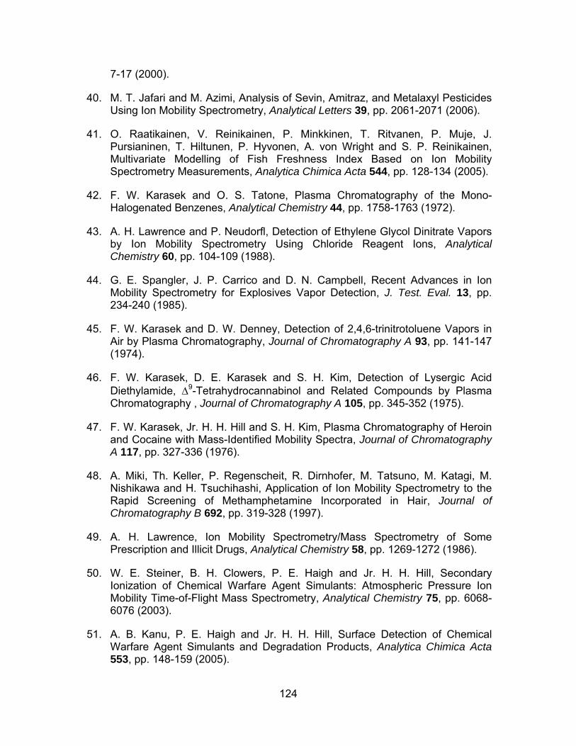
124

7-17 (2000).

40. M. T. Jafari and M. Azimi, Analysis of Sevin, Amitraz, and Metalaxyl Pesticides Using Ion Mobility Spectrometry, Analytical Letters 39, pp. 2061-2071 (2006).

41. O. Raatikainen, V. Reinikainen, P. Minkkinen, T. Ritvanen, P. Muje, J. Pursianinen, T. Hiltunen, P. Hyvonen, A. von Wright and S. P. Reinikainen, Multivariate Modelling of Fish Freshness Index Based on Ion Mobility Spectrometry Measurements, Analytica Chimica Acta 544, pp. 128-134 (2005).

42. F. W. Karasek and O. S. Tatone, Plasma Chromatography of the Mono-Halogenated Benzenes, Analytical Chemistry 44, pp. 1758-1763 (1972).

43. A. H. Lawrence and P. Neudorfl, Detection of Ethylene Glycol Dinitrate Vapors by Ion Mobility Spectrometry Using Chloride Reagent Ions, Analytical Chemistry 60, pp. 104-109 (1988).

44. G. E. Spangler, J. P. Carrico and D. N. Campbell, Recent Advances in Ion Mobility Spectrometry for Explosives Vapor Detection, J. Test. Eval. 13, pp. 234-240 (1985).

45. F. W. Karasek and D. W. Denney, Detection of 2,4,6-trinitrotoluene Vapors in Air by Plasma Chromatography, Journal of Chromatography A 93, pp. 141-147 (1974).

46. F. W. Karasek, D. E. Karasek and S. H. Kim, Detection of Lysergic Acid Diethylamide, Δ9-Tetrahydrocannabinol and Related Compounds by Plasma Chromatography , Journal of Chromatography A 105, pp. 345-352 (1975).

47. F. W. Karasek, Jr. H. H. Hill and S. H. Kim, Plasma Chromatography of Heroin and Cocaine with Mass-Identified Mobility Spectra, Journal of Chromatography A 117, pp. 327-336 (1976).

48. A. Miki, Th. Keller, P. Regenscheit, R. Dirnhofer, M. Tatsuno, M. Katagi, M. Nishikawa and H. Tsuchihashi, Application of Ion Mobility Spectrometry to the Rapid Screening of Methamphetamine Incorporated in Hair, Journal of Chromatography B 692, pp. 319-328 (1997).

49. A. H. Lawrence, Ion Mobility Spectrometry/Mass Spectrometry of Some Prescription and Illicit Drugs, Analytical Chemistry 58, pp. 1269-1272 (1986).

50. W. E. Steiner, B. H. Clowers, P. E. Haigh and Jr. H. H. Hill, Secondary Ionization of Chemical Warfare Agent Simulants: Atmospheric Pressure Ion Mobility Time-of-Flight Mass Spectrometry, Analytical Chemistry 75, pp. 6068-6076 (2003).


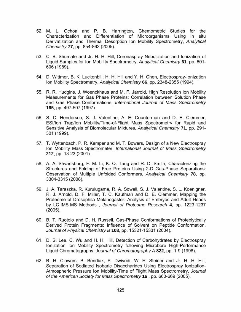
125

52. M. L. Ochoa and P. B. Harrington, Chemometric Studies for the Characterization and Differentiation of Microorganisms Using in situ Derivatization and Thermal Desorption Ion Mobility Spectrometry, Analytical Chemistry 77, pp. 854-863 (2005).

53. C. B. Shumate and Jr. H. H. Hill, Coronaspray Nebulization and Ionization of Liquid Samples for Ion Mobility Spectrometry, Analytical Chemistry 61, pp. 601-606 (1989).

54. D. Wittmer, B. K. Luckenbill, H. H. Hill and Y. H. Chen, Electrospray-Ionization Ion Mobility Spectrometry, Analytical Chemistry 66, pp. 2348-2355 (1994).

55. R. R. Hudgins, J. Woenckhaus and M. F. Jarrold, High Resolution Ion Mobility Measurements for Gas Phase Proteins: Correlation between Solution Phase and Gas Phase Conformations, International Journal of Mass Spectrometry 165, pp. 497-507 (1997).

56. S. C. Henderson, S. J. Valentine, A. E. Counterman and D. E. Clemmer, ESI/Ion Trap/Ion Mobility/Time-of-Flight Mass Spectrometry for Rapid and Sensitive Analysis of Biomolecular Mixtures, Analytical Chemistry 71, pp. 291-301 (1999).

57. T. Wyttenbach, P. R. Kemper and M. T. Bowers, Design of a New Electrospray Ion Mobility Mass Spectrometer, International Journal of Mass Spectrometry 212, pp. 13-23 (2001).

58. A. A. Shvartsburg, F. M. Li, K. Q. Tang and R. D. Smith, Characterizing the Structures and Folding of Free Proteins Using 2-D Gas-Phase Separations: Observation of Multiple Unfolded Conformers, Analytical Chemistry 78, pp. 3304-3315 (2006).

59. J. A. Taraszka, R. Kurulugama, R. A. Sowell, S. J. Valentine, S. L. Koenigner, R. J. Arnold, D. F. Miller, T. C. Kaufman and D. E. Clemmer, Mapping the Proteome of Drosophila Melanogaster: Analysis of Embryos and Adult Heads by LC-IMS-MS Methods , Journal of Proteome Research 4, pp. 1223-1237 (2005).

60. B. T. Ruotolo and D. H. Russell, Gas-Phase Conformations of Proteolytically Derived Protein Fragments: Influence of Solvent on Peptide Conformation, Journal of Physical Chemistry B 108, pp. 15321-15331 (2004).

61. D. S. Lee, C. Wu and H. H. Hill, Detection of Carbohydrates by Electrospray Ionization Ion Mobility Spectrometry following Microbore High-Performance Liquid Chromatography, Journal of Chromatography A 822, pp. 1-9 (1998).

62. B. H. Clowers, B. Bendiak, P. Dwivedi, W. E. Steiner and Jr. H. H. Hill, Separation of Sodiated Isobaric Disaccharides Using Electrospray Ionization-Atmospheric Pressure Ion Mobility-Time of Flight Mass Spectrometry, Journal of the American Society for Mass Spectrometry 16 , pp. 660-669 (2005).

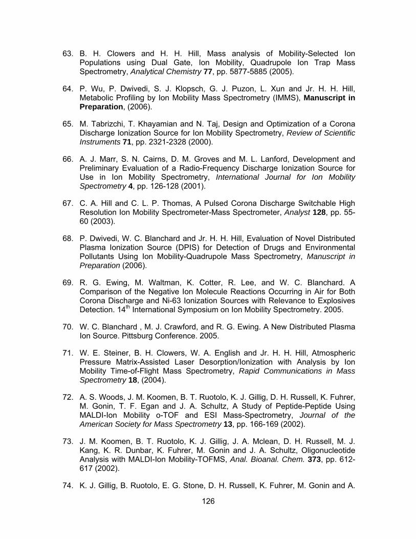
126

63. B. H. Clowers and H. H. Hill, Mass analysis of Mobility-Selected Ion Populations using Dual Gate, Ion Mobility, Quadrupole Ion Trap Mass Spectrometry, Analytical Chemistry 77, pp. 5877-5885 (2005).

64. P. Wu, P. Dwivedi, S. J. Klopsch, G. J. Puzon, L. Xun and Jr. H. H. Hill, Metabolic Profiling by Ion Mobility Mass Spectrometry (IMMS), Manuscript in Preparation, (2006).

65. M. Tabrizchi, T. Khayamian and N. Taj, Design and Optimization of a Corona Discharge Ionization Source for Ion Mobility Spectrometry, Review of Scientific Instruments 71, pp. 2321-2328 (2000).

66. A. J. Marr, S. N. Cairns, D. M. Groves and M. L. Lanford, Development and Preliminary Evaluation of a Radio-Frequency Discharge Ionization Source for Use in Ion Mobility Spectrometry, International Journal for Ion Mobility Spectrometry 4, pp. 126-128 (2001).

67. C. A. Hill and C. L. P. Thomas, A Pulsed Corona Discharge Switchable High Resolution Ion Mobility Spectrometer-Mass Spectrometer, Analyst 128, pp. 55-60 (2003).

68. P. Dwivedi, W. C. Blanchard and Jr. H. H. Hill, Evaluation of Novel Distributed Plasma Ionization Source (DPIS) for Detection of Drugs and Environmental Pollutants Using Ion Mobility-Quadrupole Mass Spectrometry, Manuscript in Preparation (2006).

69. R. G. Ewing, M. Waltman, K. Cotter, R. Lee, and W. C. Blanchard. A Comparison of the Negative Ion Molecule Reactions Occurring in Air for Both Corona Discharge and Ni-63 Ionization Sources with Relevance to Explosives Detection. 14th International Symposium on Ion Mobility Spectrometry. 2005.

70. W. C. Blanchard , M. J. Crawford, and R. G. Ewing. A New Distributed Plasma Ion Source. Pittsburg Conference. 2005.

71. W. E. Steiner, B. H. Clowers, W. A. English and Jr. H. H. Hill, Atmospheric Pressure Matrix-Assisted Laser Desorption/Ionization with Analysis by Ion Mobility Time-of-Flight Mass Spectrometry, Rapid Communications in Mass Spectrometry 18, (2004).

72. A. S. Woods, J. M. Koomen, B. T. Ruotolo, K. J. Gillig, D. H. Russell, K. Fuhrer, M. Gonin, T. F. Egan and J. A. Schultz, A Study of Peptide-Peptide Using MALDI-Ion Mobility o-TOF and ESI Mass-Spectrometry, Journal of the American Society for Mass Spectrometry 13, pp. 166-169 (2002).

73. J. M. Koomen, B. T. Ruotolo, K. J. Gillig, J. A. Mclean, D. H. Russell, M. J. Kang, K. R. Dunbar, K. Fuhrer, M. Gonin and J. A. Schultz, Oligonucleotide Analysis with MALDI-Ion Mobility-TOFMS, Anal. Bioanal. Chem. 373, pp. 612-617 (2002).

74. K. J. Gillig, B. Ruotolo, E. G. Stone, D. H. Russell, K. Fuhrer, M. Gonin and A.

127

J. Schultz, Coupling High-Pressure MALDI with Ion Mobility/Orthogonal Time-of-Flight Mass Spectrometry, Analytical Chemistry 72, pp. 3965-3971 (2000).

75. J. Gidden, M. T. Bowers, A. T. Jackson and J. H. Scrivens, Gas-Phase Conformations of Cationized Poly(styrene) Oligomers, Journal of the American Society for Mass Spectrometry 13, pp. 499-505 (2002).

76. S. Lee, T. Wyttenbach and M. T. Bowers, Gas-Phase Structures of Sodiated Oligosaccharides by Ion Mobility Ion Chromatography Methods, International Journal of Mass Spectrometry 167, pp. 605-614 (1997).

77. Y. Lu, F. Zhou, W. Shui, L. Bian, Y. Guo and P. Yang, Pulsed Electrospray for Mass Spectrometry, Analytical Chemistry 73, pp. 4748-4753 (2001).

78. L. Y. Yeo, D. Lastochkin, S. C. Wang and H. C. Chang, A New AC Electrospray Mechanism by Maxwell-Wagner Polarization and Capillary Resonance, Physical Review Letters 92, pp. 133902-1-133902-4 (2004).

79. B. F. Chao, C. J. Chen, F. A. Li and G. R. Her, Sheathless Capillary Electrophoresis-Mass Spectrometry Using a Pulsed Electrospray Ionization Source, Electrophoresis 27, pp. 2083-2090 (2006).

80. J. Wei, W. Shui, F. Zhou, Y. Lu, K. Chen, G. Xu and P. Yang, Naturally and Externally Pulsed Electrospray, Mass Spectrometry Reviews 21, pp. 148-162 (2002).


82. D. R. Lide, CRC Handbook of Chemistry and Physics (85th Edn). CRC Press, Boca Raton, FL (2004).

83. D. R. Baker, Capillary Electrophoresis. John Wiley & Sons, Inc., New York, NY (1995).

84. M. A. Baim and Jr. H. H. Hill, Tunable Selective Detection for Capillary Gas Chromatography by Ion Mobility Spectrometry, Analytical Chemistry 54, pp. 38-43 (1982).

85. P. W. Atkins, Physical Chemistry (5th Edn). W. H. Freeman and Company, USA (1994).

86. C. J. T. von Grotthuss, Sur la Décomposition de l'eau et des Corps qu'elle Tient en Dissolution ŕ l'aide de L'électricité Galvanique, Ann. Chim. LVIII, pp. 54-74 (1806).

87. M. Eigen and L. de Maeyer, Self-Dissociation and Protonic Charge Transport in Water and Ice, Proceedings of the Royal Society of London. Series A 247, pp. 505-533 (1958).

128

88. Y. Wu and G. A. Voth, A Computer Simulation Study of the Hydrated Proton in a Synthetic Proton Channel, Biophysical Journal 85, pp. 864-875 (2003).

89. U. W. Schmitt and G. A. Voth, The Computer Simulation of Proton Transfer in Water, Journal of Chemical Physics 111, pp. 9361-9381 (1999).

90. D. E. Raymond, A. Manz and H. M. Widmer, Continuous Separation of High Molecular Weight Compounds Using a Microliter Volume Free-Flow Electrophoresis Microstructure, Analytical Chemistry 68, pp. 2515-2522 (1996).

91. I. D. MacLeod, D. M. Muir, A. J. Parker and P. Singh, Solvation of Ions. Some Applications. II. Electrolysis of Copper (I) Sulphate in Water-Nitrile Mixtures, Australian Journal of Chemistry 30, pp. 1423-1437 (1977).

92. R. A. Robinson and R. H. Stokes, Electrolyte Solutions (Second Edn). Butterworths Publications Limited, London, England (1965).

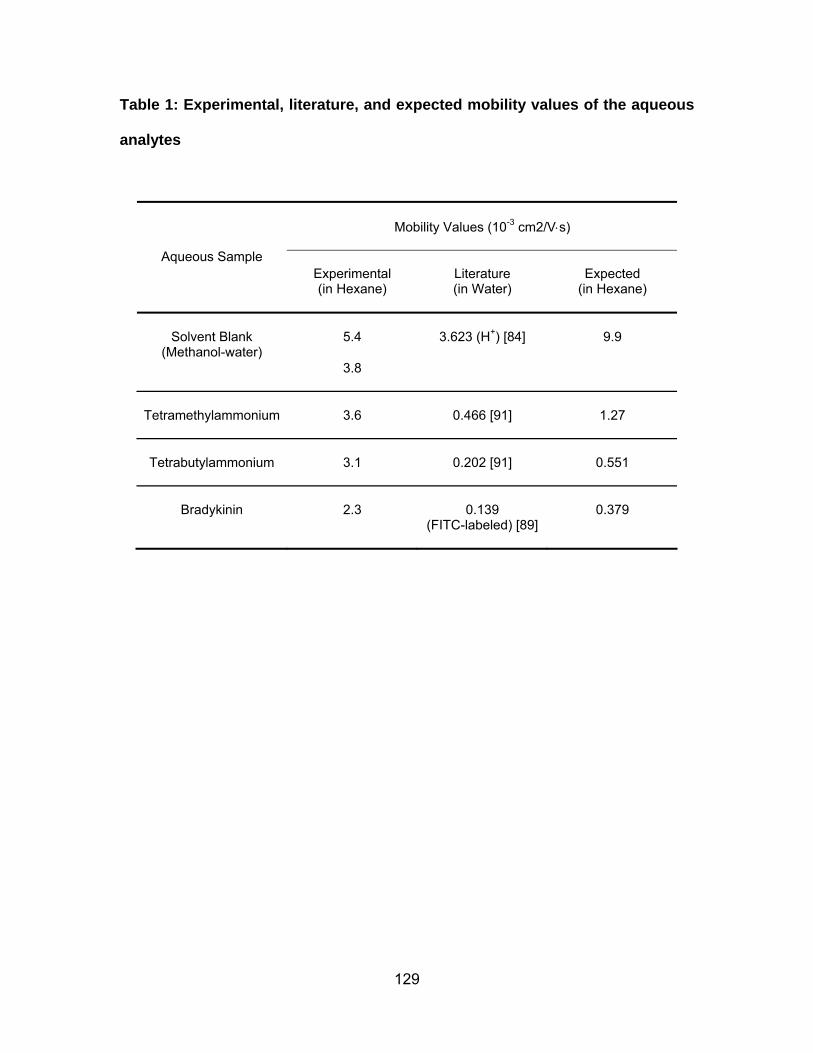
129

Table 1: Experimental, literature, and expected mobility values of the aqueous

analytes

Mobility Values (10-3 cm2/V⋅s)

Aqueous Sample Experimental (in Hexane)

Literature (in Water)

Expected

(in Hexane)

5.4

3.623 (H+) [84]

9.9

Solvent Blank

(Methanol-water) 3.8

Tetramethylammonium

3.6

0.466 [91]

1.27

Tetrabutylammonium

3.1

0.202 [91]

0.551

Bradykinin

2.3

0.139

(FITC-labeled) [89]

0.379

130

Figure Captions

Figure 1: Schematic of liquid phase ion mobility spectrometer (LPIMS) with pulsed

electrodispersion ionization (EDI). The components included a pulsed

electrodispersion ionization source, a resistive glass ion mobility spectrometer, and a

Faraday plate, all of which were rested inside a Pyrex dish filled with the liquid

medium.

Figure 2: Pulsed electrodispersion ionization – liquid phase ion mobility spectra of

the solvent blank (methanol-water, 90:10 vol/vol) for (a) the first 8.5 minutes (51

averages), (b) the final 2.5 minutes (15 averages), and (c) the entire 30 minutes (179

averages).

Figure 3: Pulsed electrodispersion ionization – liquid phase ion mobility spectra of

the solvent blank (methanol-water, 90:10 vol/vol) was obtained over 30 minutes (179

spectra) in the positive mode. The 3D plot showed that there were two populations of

ions, the first group of ions with higher current intensity (A) and the second group of

ions with lower current intensity (B).

Figure 4a: Pulsed electrodispersion ionization – liquid phase ion mobility spectrum

of 100 μM tetramethylammonium bromide in the positive mode.

Figure 4b: Pulsed electrodispersion ionization – liquid phase ion mobility spectrum

of 100 μM tetrabutylammonium bromide.

131

Figure 4c: Pulsed electrodispersion ionization – liquid phase ion mobility spectrum

of 100 μM bradykinin in the positive mode.

132

Figure 1: Schematic of liquid phase ion mobility spectrometer (LPIMS) with pulsed electrodispersion ionization (EDI). The components included a pulsed electrodispersion ionization source, a resistive glass ion mobility spectrometer, and a Faraday plate, all of which were rested inside a Pyrex dish filled with the liquid medium.

(B) Electrodispersion Ionization Source

(C) Resistive Glass Ion Mobility Spectrometer

(D) Faraday Plate (B) Pyrex Dish Filled with Liquid Medium

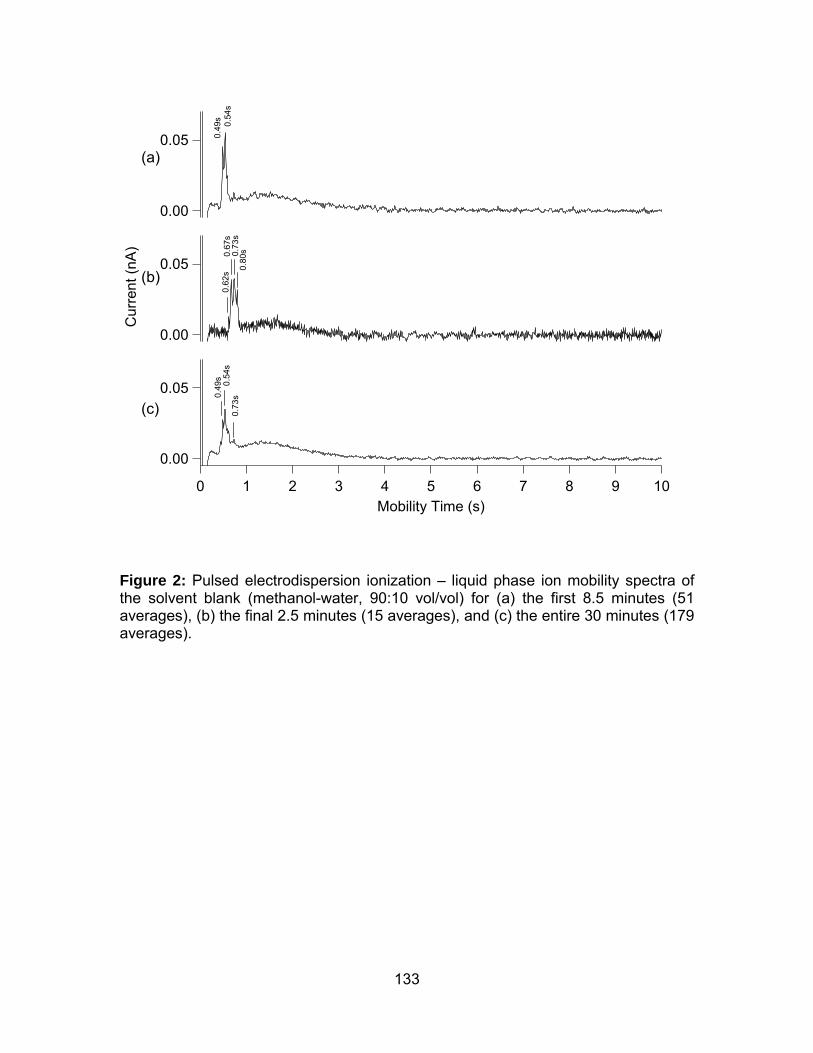
133

0.05

0.00

Cur

rent

(nA

)


0.05

0.00

0.05

0.000.

49s 0.54

s0.

62s

0.67

s

0.80

s0.73

s

0.49

s 0.54

s0.

73s

Figure 2: Pulsed electrodispersion ionization – liquid phase ion mobility spectra of the solvent blank (methanol-water, 90:10 vol/vol) for (a) the first 8.5 minutes (51 averages), (b) the final 2.5 minutes (15 averages), and (c) the entire 30 minutes (179 averages).

(a)

(b)

(c)

134

Figure 3: Pulsed electrodispersion ionization – liquid phase ion mobility spectra of the solvent blank (methanol-water, 90:10 vol/vol) was obtained over 30 minutes (179 spectra) in the positive mode. The 3D plot showed that there were two populations of ions, the first group of ions with higher current intensity (A) and the second group of ions with lower current intensity (B).

Cur

rent

(nA

)

Spectrum N

umber

A

B

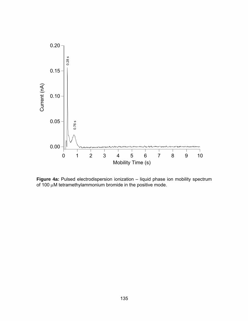
135

0.20

0.15

0.10

0.05

0.00

Cur

rent

(nA)


0.76

s

0.28

s

Figure 4a: Pulsed electrodispersion ionization – liquid phase ion mobility spectrum of 100 μM tetramethylammonium bromide in the positive mode.

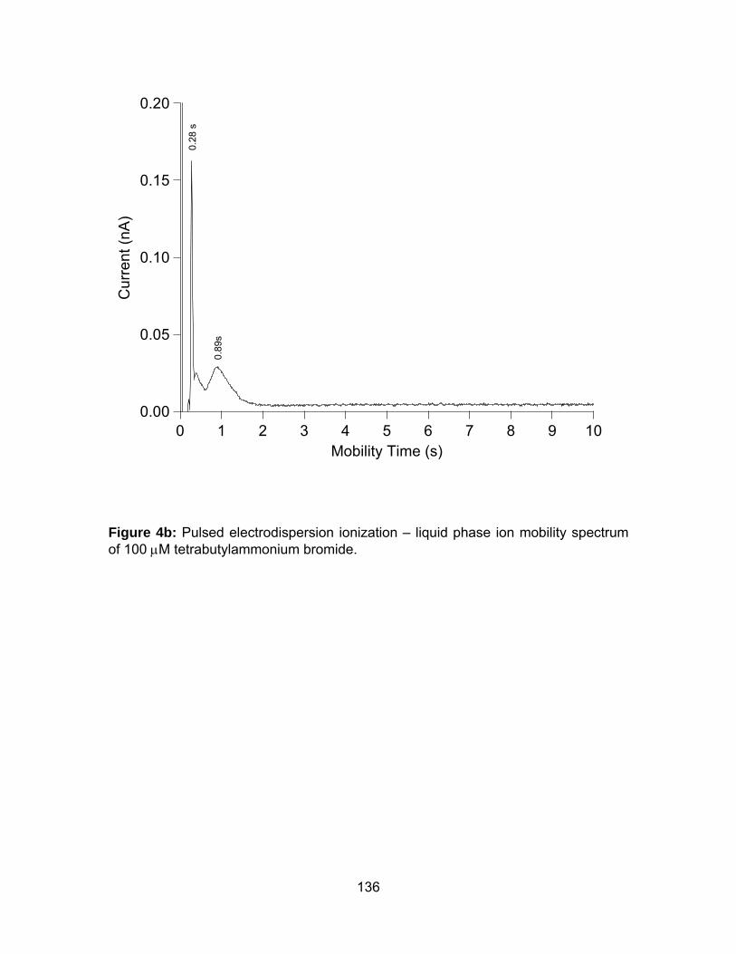
136

0.20

0.15

0.10

0.05

0.00

Cur

rent

(nA)


0.89

s

0.28

s

Figure 4b: Pulsed electrodispersion ionization – liquid phase ion mobility spectrum of 100 μM tetrabutylammonium bromide.

137

0.25

0.20

0.15

0.10

0.05

0.00

Cur

rent

(nA)


1.18

s

0.67

s

Figure 4c: Pulsed electrodispersion ionization – liquid phase ion mobility spectrum of 100 μM bradykinin in the positive mode.

138

Chapter Six

Conclusions

Portable devices based on gas phase ion mobility spectrometry are widely employed

by first responders for the rapid detection of explosives and warfare agents because

of its simple instrumentation, low maintenance, and milliseconds-fast analysis time.

However, improving separation efficiency has been especially challenging in

miniaturized IMS. The maximum attainable resolving power is proportional to the

square root of the IMS drift length. Therefore, separation power of IMS suffers at the

expense of miniaturization. With the concept of the maximum resolving power also

being proportional to the square root of the operational pressure, this project

introduced a novel analytical method, called liquid phase ion mobility spectrometry.

139

i) Electrodispersion ionization was developed as a suitable ionization source

for liquid phase ion mobility spectrometry.

Prior to the development of liquid phase ion mobility spectrometry (LPIMS), it was

critical to identify a suitable ionization source. Without an appropriate ion source,

LPIMS, whose separation and detection required the conversion of the analytes into

charged particles, could not be demonstrated. The potential ionization source should

have the capability to ionize aqueous solution of analytes in a non-electrolyte

containing liquid medium. Since the measurement of discharge current by Faraday

plate was the intended detection method, the ionization source should selectively

ionize the aqueous analyte, and not the liquid medium. Additionally, it would be ideal

for the ionization source to be non-radioactive. The inclusion of radioactive material

and generation of radioactive waste would hinder the implementation of LPIMS as a

portable and rapid personal diagnostic tool.

A new ionization source, called electrodispersion ionization, was developed to

address these criteria. EDI produced ions from aqueous phase analytes in non-

electrolyte containing liquids. EDI was effective in delivering pre-existent positive and

negative ions from aqueous sample solution and dispersing them into the organic

liquid medium. Its ionization efficiency was dependent upon the sample flow rate.

Visualization of the electrodispersed droplets was demonstrated with aqueous

solutions of two dyes, basic fuchsin and bromothymol blue. Continuous and stable

current from EDI was measured for inorganic and organic ions by Faraday plate.

Quantitative ionization of the method was investigated for several amino acids with

detection limits measured in the low ppm range.

140

Under certain operation conditions, combinations of applied voltage and sample flow

rate can lead to pulsing of the ion current for the EDI source. Control of this pulsing

phenomenon may lead to the elimination of the need for an ion gate in such

applications as liquid phase ion mobility spectrometry. EDI may be especially useful

in combination with liquid phase ion mobility spectrometry and other liquid phase

separation methods for ions. In addition, EDI may be useful for the creation of ions

or the dispersion of reactants into non-aqueous phases for chemical syntheses.

141

ii) Ion transport in liquid phase ion mobility spectrometry was demonstrated.

Efficiency of Bradbury-Nielsen shutter and Tyndall shutter were

investigated in the liquid phase.

Ions produced from EDI were were moved along by an electric field along the LPIMS

in a liquid medium. Liquid phase ion mobility spectrometry with electrodispersion

ionization was demonstrated for the first time. The LPIMS spectra of ammonium

nitrate and sodium chloride were inadequately resolved possibly due to the

extension of analyte solvation and the inefficiency of the ion shutters.

The efficiency of two types of ion shutters, Tyndall and Bradbury-Nielsen shutters,

for LPIMS was investigated. The total ion current leaking pass the ion shutters

decreased with increasing orthogonal field of Bradbury-Nielsen shutter and with

increasing reverse field of Tyndall gate. 95% of the total ion could be stopped with

an orthogonal field 32 times greater and a reverse field 8.5 times greater than the

electric field of the LPIMS for the Bradbury-Nielsen shutter and Tyndall shutter,

respectively.

142

iii) Integrated system of liquid phase ion mobility spectrometry were designed,

constructed, and evaluated.

Directing the research towards the ultimate goal of using LPIMS as a personal

diagnostic tool, attempts were made to integrate the components of LPIMS into an

inexpensive and disposable composite device which could be mass produced cost

effectively. New instrument designs and alternative fabrication processes were

explored: low temperature co-fired ceramics (LTCC) and poly(dimethylsiloxane)

(PDMS) fabricated with Micro-Electro-Mechanical Systems technology. 90 sheets of

LTCC sheet, with embedded conducting electrodes and resistors, were fused into a

single LTCC-LPIMS device. The electrical connections for LTCC-LPIMS were limited

to only five inputs and outputs. The instrumental parts and fabrication process time

of LPIMS were further reduced with the incorporation of the EDI source into the

PDMS-LPIMS. Identical PDMS-LPIMS microchannels could be replicated with ease

after a master, which carried a positive relief of the LPIMS microchannel pattern,

was patterned. Ion transport efficiency was a major issue for both LTCC-LPIMS and

PDMS-LPIMS that needed to be solve.

143

iv) Liquid phase ion mobility spectrometry with pulsed electrodispersion

ionization was demonstrated.

As with other time-of-flight analyzer, it was anticipated that LPIMS would interface

well with a pulsed ionization source. The use of a pulsed ionization eliminated the

need for an ion shutter in LPIMS and thus simplifying the fabrication process. A

pulsed ionization source also required smaller sample volumes.

Previous experiments showed that pulsing of the ion current for the EDI source was

controlled by combinations of applied voltage and sample flow rate. Pulsed EDI was

achieved by alternating the voltage applied to the ionization source, between a

voltage sufficient to induce electrodispersion and a lower voltage. Pulsed EDI-LPIMS

of methanol-water solvent blank in hexane showed that the amount of solvation for

the solvent ions increased with experimental duration. This suggested the necessity

of a counter flowing liquid medium for the removal of uncharged molecule in the

LPIMS. Mobility values of tetramethylammonium, tetrabutylammonium, and

bradykinin, obtained from pulsed EDI-LPIMS spectra, were three to five times faster

than those predicted for singly charged analyte in hexane. It was speculated that the

absence of ion-dipole interaction between the ions and the non-polar hexane

displaced the solvation sphere that would otherwise exist in aqueous solution.

APPENDIX

145

Appendix I

Additional Data from Parametric Studies of

Electrodispersion Ionization

146

Figure Captions

Figure 1: Schematic of the electrodispersion ionization apparatus.

Figure 2: Plot of total ion current versus electrodispersion ionization voltage for

sample of methanol-water and 100 μM ammonium chloride at a flow rate of 0.1

μL/min in benzene and decane, in the positive mode. The total ion current increased

with EDI voltage. The onset voltage of EDI was 300V, 250V, 400V, and 450V, for

methanol-water in benzene, ammonium chloride in benzene, methanol-water in

decane, and ammonium chloride in decane, respectively.

Figure 3: Effect of sample flow rate on electrodispersion ionization efficiency for a

sample of methanol-water (90:10) in benzene. The sample flow rate studied were

0.05 μL/min ( ), 0.1 μL/min ( ), 0.2 μL/min ( ), and 0.5 μL/min ( ).


sample of methanol-water (90:10) and 100 μM ammonium chloride, in benzene and

decane. The range of sample flow rates was from 0.02 μL/min to 2.0 μL/min. The

EDI voltage was +750V.


sample of methanol-water (90:10) and 100 μM ammonium chloride, in benzene and

decane. The sample flow rate studied were from 0.02 μL/min to 2.0 μL/min. The EDI

voltage was -750V.

147

Figure 1: Schematic of the electrodispersion ionization apparatus.

(D) Fused Silica Capillary

(C) PTFE/Silicone Septum

(B) Open Top Screw Cap

(E) Faraday Plate

(A) Pyrex Culture Tube

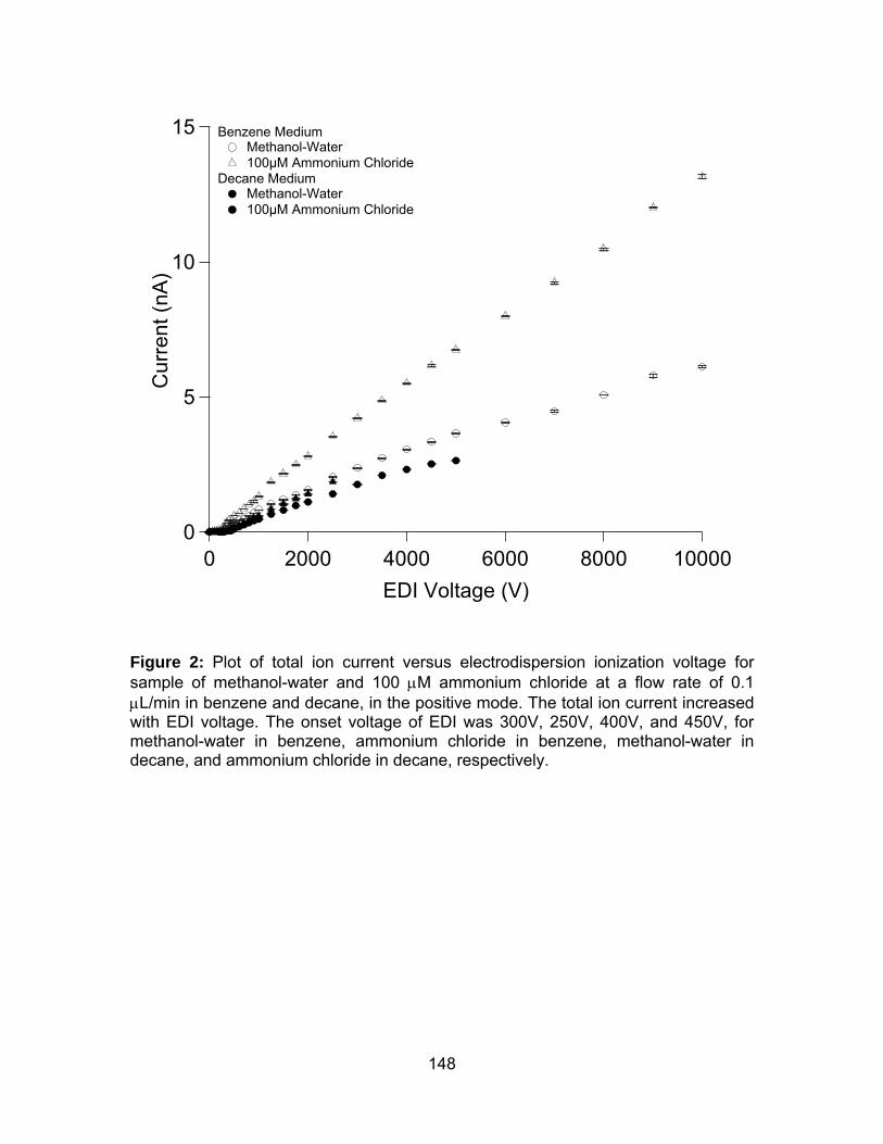
148

15

10

5

0

Cur

rent

(nA

)

1000080006000400020000EDI Voltage (V)

Benzene MediumMethanol-Water100µM Ammonium Chloride

Decane MediumMethanol-Water100µM Ammonium Chloride

Figure 2: Plot of total ion current versus electrodispersion ionization voltage for sample of methanol-water and 100 μM ammonium chloride at a flow rate of 0.1 μL/min in benzene and decane, in the positive mode. The total ion current increased with EDI voltage. The onset voltage of EDI was 300V, 250V, 400V, and 450V, for methanol-water in benzene, ammonium chloride in benzene, methanol-water in decane, and ammonium chloride in decane, respectively.

149

0

1

2

3

4

5

0 1000 2000 3000 4000 5000 6000 7000 8000 9000 10000

Applied Voltage

Cur

rent

(nA

)

Figure 3: Effect of sample flow rate on electrodispersion ionization efficiency for a sample of methanol-water (90:10) in benzene. The sample flow rate studied were 0.05 μL/min ( ), 0.1 μL/min ( ), 0.2 μL/min ( ), and 0.5 μL/min ( ).

150

1.5

1.0

0.5

0.0

Cur

rent

(nA

)

2.01.51.00.5Sample Flow Rate (µL/min)

Benzene MediumMethanol-Water 100 µM Ammonium Chloride

Decane MediumMethanol-Water 100 µM Ammonium Chloride

Figure 4: Effect of sample flow rate on electrodispersion ionization efficiency for a sample of methanol-water (90:10) and 100 μM ammonium chloride, in benzene and decane. The range of sample flow rates was from 0.02 μL/min to 2.0 μL/min. The EDI voltage was +750V.

151

1.5

1.0

0.5

0.0

Cur

rent

(nA

)

2.01.51.00.5Sample Flow Rate (µL/min)

Benzene Medium100 µM Ammonium Chloride

Decane MediumMethanol-Water 100 µM Ammonium Chloride

Figure 5: Effect of sample flow rate on electrodispersion ionization efficiency for a sample of methanol-water (90:10) and 100 μM ammonium chloride, in benzene and decane. The sample flow rate studied were from 0.02 μL/min to 2.0 μL/min. The EDI voltage was -750V.

152

Appendix II

Additional Graphic Representations of Liquid

Phase Ion Mobility Spectrometers

153

Figure Captions

Figure 1: Liquid phase ion mobility spectrometer (LPIMS), constructed from a Pyrex

culture tube. The electric field was established by multiple stainless steel electrodes

connected in series with resistors. The photograph also showed the sample inlet,

liquid medium inlet and outlet, and the electrical connections.

Figure 2: Mobility tube of LPIMS, fabricated from low temperature co-fired ceramic

(LTCC). The photograph showed that the diameter of the device was smaller than

that of a quarter.

Figure 3: The complete prototype of low temperature co-fired ceramic-liquid phase

ion mobility spectrometer (LTCC-LPIMS): photograph displaying the LPIMS mobility

tube (A), the sealing Teflon end caps (B – D), the external electrical connections (E),

the liquid medium entry (F), and the liquid medium exit (G). The three pieces of

Teflon end caps were physically tightened with three screws and sealed with two

pieces of o-rings and a membrane that fitted into the counter bore of the end caps.

Figure 4: Schematic of the LTCC-LPIMS prototype, showing (A) the internal

electrical connections, and (B) the alignment holes and the external electrical

connections: (1) aperture grid, where the spectrometer voltage was grounded via an

external resistor, (2) ion shutter sense line, (3) ion shutter voltage input, (4)

spectrometer voltage input, and (5) Faraday plate.

154

Figure 5: Photograph of the first generation of poly(dimethylsiloxane)-liquid phase

ion mobility spectrometer (PDMS-LPIMS). The PDMS-LPIMS microchannel was

1000 μm wide, 400 μm deep, and 5 cm long. There were 24 sputtered gold

electrodes. The sample inlet was a fused silica capillary inserted at the front end of

the LPIMS-PDMS.

Figure 6: Photograph of the second generation of poly(dimethylsiloxane)-liquid

phase ion mobility spectrometer (PDMS-LPIMS). The PDMS channel was 1000 μm

wide, 400 μm deep and 5 cm long. There were 26 machine-sputtered gold

electrodes. The sample inlet and the drift liquid inlet were polyethylene tubing,

located at the front and back end of the PDMS channel. Electrical wires were

connected to each of the 26 gold electrodes with conducting silver paste.

Figure 7: Three-dimensional schematic of the third generation of PDMS-LPIMS. The

PDMS channel was 1000 μm wide, 400 μm deep and 1 cm long. The sample inlet

was incorporated into the PDMS design.

Figure 8: Top-view schematic of the third generation of PDMS-LPIMS. The

microchannel was 1000 μm wide, 400 μm deep and 1 cm long. There were 6

sputtered platinum electrodes. EDI voltage was applied at electrode 0. The sample

nozzle was incorporated into the PDMS design near electrode 1. Electrode 6 was

used as the Faraday plate.

155

Figure 9: Photograph of the fourth generation of PDMS-LPIMS prototype, showing

the polyethylene capillaries, which carried in the liquid medium and sample, and the

electrical connections. The bottom PDMS layer was bonded to a glass microscope

slide for additional support.

Figure 10: Photograph of a resistive glass-LPIMS. A miniature Bradbury-Nielsen

gate was inserted between two resistive glass tubes, one being used as the

desolvation region and another for the drift region. The sample was introduced via a

fused silica capillary and ionized by electrodispersion ionization. The instrument was

held steady by a poly(dimethylsiloxane) cover, and immersed into a Pyrex beaker

filled with the liquid medium.

Figure 11: Photograph of the miniaturized Bradbury-Nielsen gate, with a 4.56 mm

i.d., 9.30 mm o.d., and a wire spacing of 0.64 mm.

156

Figure 1: Liquid phase ion mobility spectrometer (LPIMS), constructed from a Pyrex culture tube. The electric field was established by multiple stainless steel electrodes connected in series with resistors. The photograph also showed the sample inlet, liquid medium inlet and outlet, and the electrical connections.

LIQUID MEDIUM OUTLET

SPECTROMETER VOLTAGE

CONNECTION

PYREX DRIFT TUBE

GATE CONNECTION

LIQUID MEDIUM INLET

DETECTOR CONNECTION

GROUND CONNECTION

AQUEOUS SAMPLE OUTLET

IONIZATION VOLTAGE

CONNECTION

157

Figure 2: Mobility tube of LPIMS, fabricated from low temperature co-fired ceramic (LTCC). The photograph showed that the diameter of the device was smaller than that of a quarter.

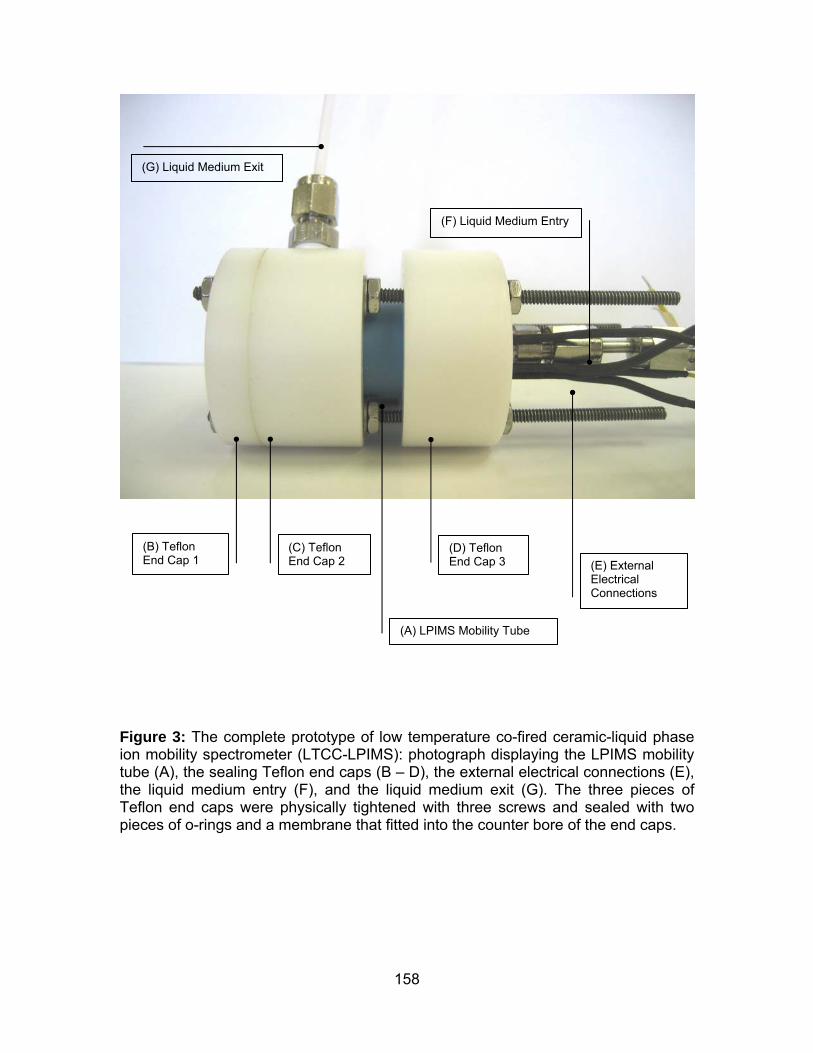
158

Figure 3: The complete prototype of low temperature co-fired ceramic-liquid phase ion mobility spectrometer (LTCC-LPIMS): photograph displaying the LPIMS mobility tube (A), the sealing Teflon end caps (B – D), the external electrical connections (E), the liquid medium entry (F), and the liquid medium exit (G). The three pieces of Teflon end caps were physically tightened with three screws and sealed with two pieces of o-rings and a membrane that fitted into the counter bore of the end caps.

(B) Teflon End Cap 1

(C) Teflon End Cap 2

(D) Teflon End Cap 3 (E) External

Electrical Connections

(G) Liquid Medium Exit

(F) Liquid Medium Entry

(A) LPIMS Mobility Tube

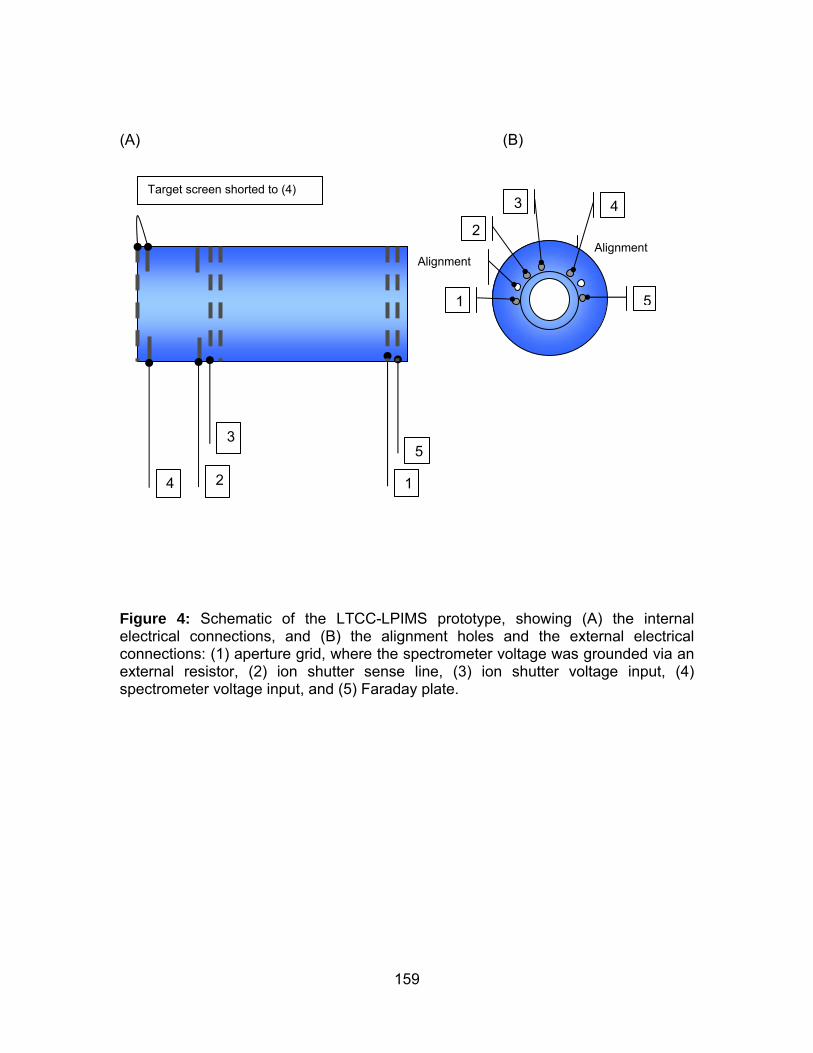
159

(A) (B)

Figure 4: Schematic of the LTCC-LPIMS prototype, showing (A) the internal electrical connections, and (B) the alignment holes and the external electrical connections: (1) aperture grid, where the spectrometer voltage was grounded via an external resistor, (2) ion shutter sense line, (3) ion shutter voltage input, (4) spectrometer voltage input, and (5) Faraday plate.

Alignment

4 2

5

1

3

Target screen shorted to (4)

5

4 3

2

1

Alignment

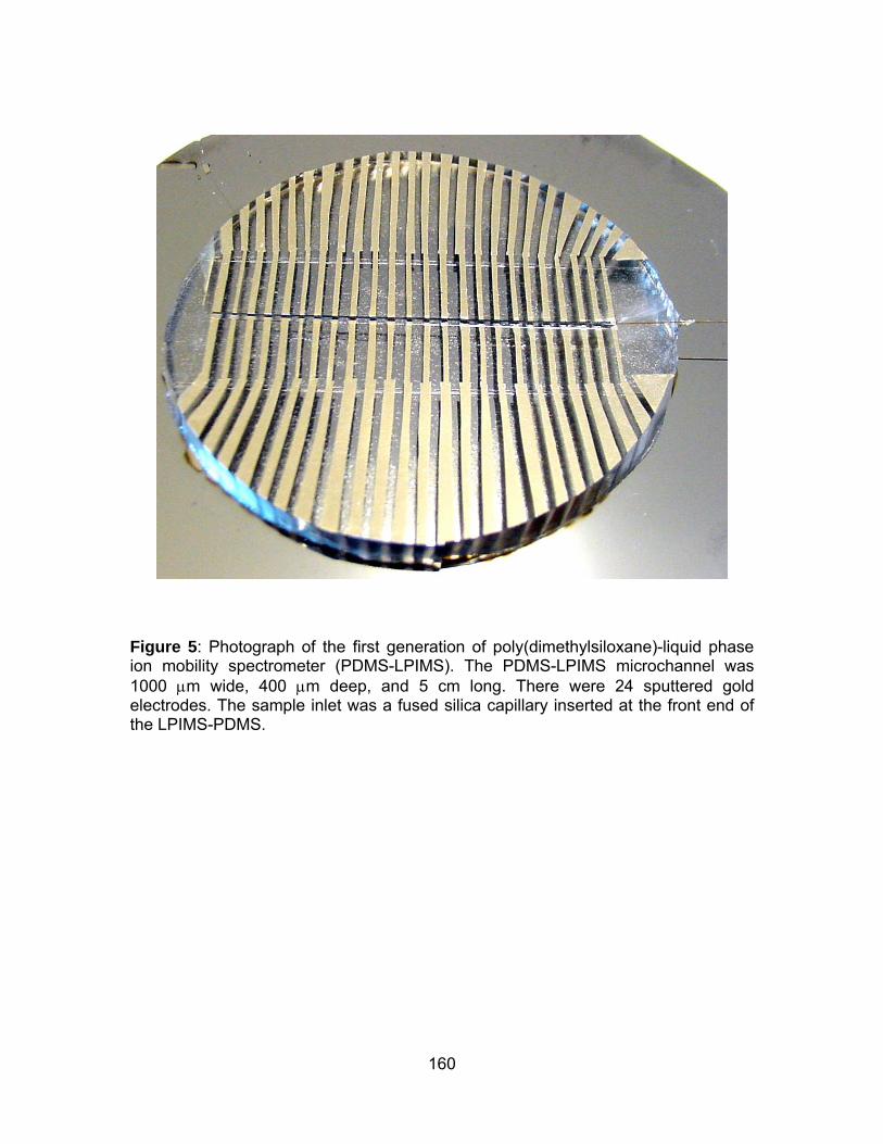
160

Figure 5: Photograph of the first generation of poly(dimethylsiloxane)-liquid phase ion mobility spectrometer (PDMS-LPIMS). The PDMS-LPIMS microchannel was 1000 μm wide, 400 μm deep, and 5 cm long. There were 24 sputtered gold electrodes. The sample inlet was a fused silica capillary inserted at the front end of the LPIMS-PDMS.

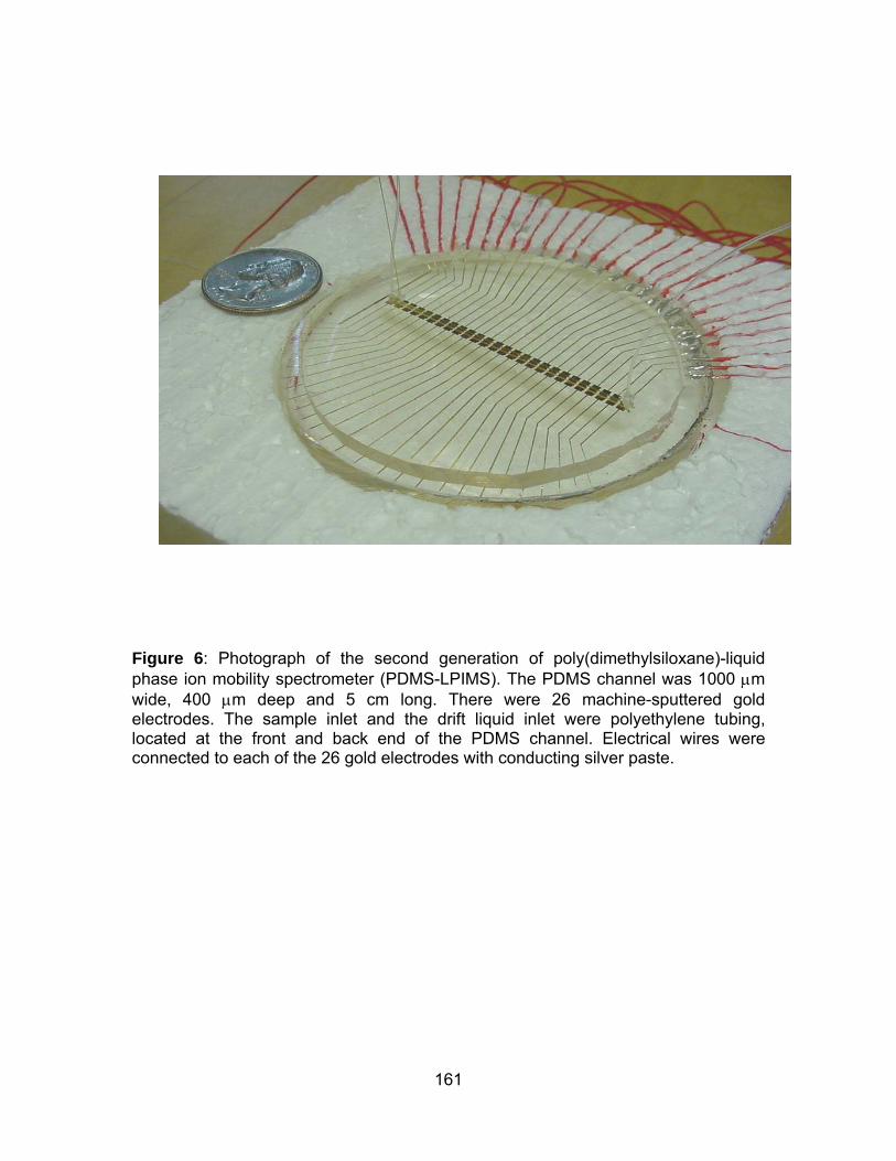
161

Figure 6: Photograph of the second generation of poly(dimethylsiloxane)-liquid phase ion mobility spectrometer (PDMS-LPIMS). The PDMS channel was 1000 μm wide, 400 μm deep and 5 cm long. There were 26 machine-sputtered gold electrodes. The sample inlet and the drift liquid inlet were polyethylene tubing, located at the front and back end of the PDMS channel. Electrical wires were connected to each of the 26 gold electrodes with conducting silver paste.

162

Figure 7: Three-dimensional schematic of the third generation of PDMS-LPIMS. The PDMS channel was 1000 μm wide, 400 μm deep and 1 cm long. The sample inlet was incorporated into the PDMS design.

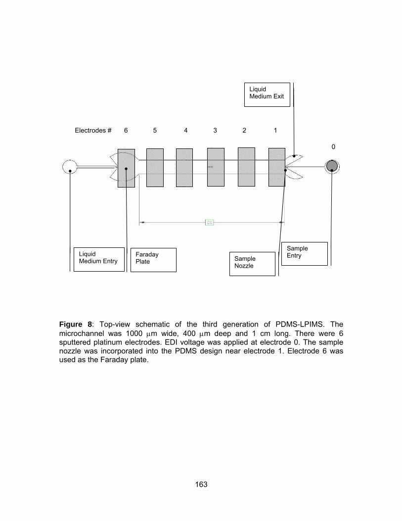
163

Figure 8: Top-view schematic of the third generation of PDMS-LPIMS. The microchannel was 1000 μm wide, 400 μm deep and 1 cm long. There were 6 sputtered platinum electrodes. EDI voltage was applied at electrode 0. The sample nozzle was incorporated into the PDMS design near electrode 1. Electrode 6 was used as the Faraday plate.

Electrodes # 6 5 4 3 2 1

0

Liquid Medium Entry

Liquid Medium Exit

Sample Entry Sample

Nozzle

Faraday Plate

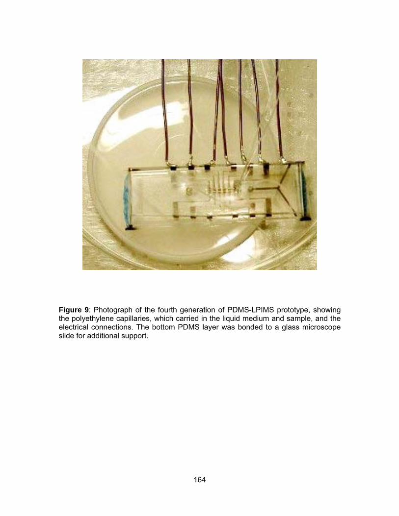
164

Figure 9: Photograph of the fourth generation of PDMS-LPIMS prototype, showing the polyethylene capillaries, which carried in the liquid medium and sample, and the electrical connections. The bottom PDMS layer was bonded to a glass microscope slide for additional support.

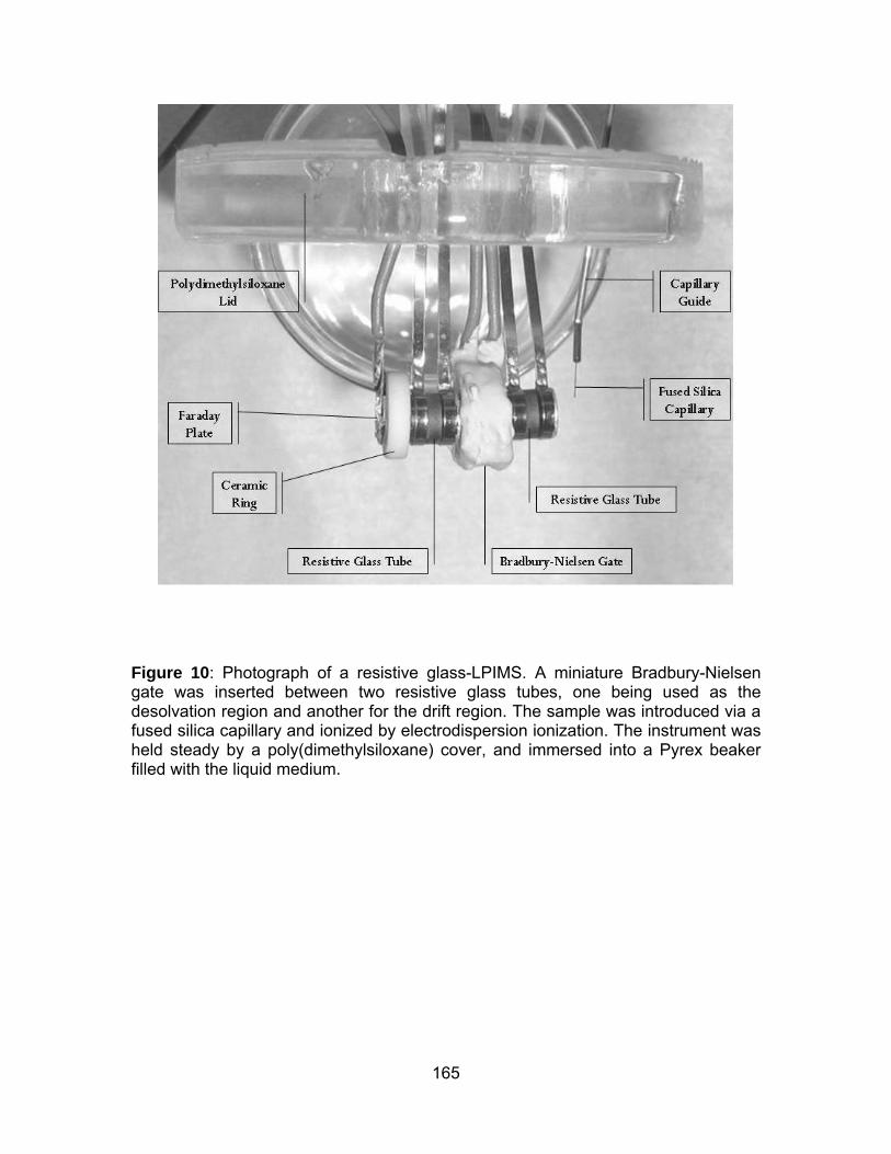
165

Figure 10: Photograph of a resistive glass-LPIMS. A miniature Bradbury-Nielsen gate was inserted between two resistive glass tubes, one being used as the desolvation region and another for the drift region. The sample was introduced via a fused silica capillary and ionized by electrodispersion ionization. The instrument was held steady by a poly(dimethylsiloxane) cover, and immersed into a Pyrex beaker filled with the liquid medium.

166

Figure 11: Photograph of the miniaturized Bradbury-Nielsen gate, with a 4.56 mm i.d., 9.30 mm o.d., and a wire spacing of 0.64 mm.

167

Appendix III

Electric Circuit for Pulsed Electrodispersion

Ionization Source

The electrical connections for pulsed electrodispersion ionization was shown in

Figure 1. Aqueous sample was introduced by a syringe pump. The syringe was

connected to a fused silica capillary through a grounded metal union. EDI voltage

was applied to the second metal union. A micro-elbow junction allowed a 90° bend of

the capillary. The pulsing of the electrodispersion ionization source was controlled by

a Double Pole Single Throw (DPST) two-way switch, designed and constructed by

Technical Services at Washington State University. The two-way switch consisted of

two reed switches (HSR-10K, Hermetic Switch Inc., Chickasha, OK), current coils,

electronic circuits and supporting power supplies. The function of two-way switch

was to alter the voltage applied to the electrodispersion ionization source between a

voltage high enough to cause electrodispersion and a lower voltage. The two-way

switch was also used for controlling the voltage applied to the ion shutter. The

schematic of the two-way switch circuit and the electrical connections for pulsed

electrodispersion ionization was shown in Figure 1.

168

The HSR-10K reed switch could toggle voltages up to a maximum of 10 kV. Each

reed switch had two overlapping ferromagnetic reeds with tungsten contacts,

hermetically sealed inside a glass capsule. A coil of wire wrapped around the glass

capsule (187 turns). Contact between the two reeds was made by a magnetic field,

generated by passing a current through the coil. The two reeds “bounced” when the

contact was made and a steady state was reached within 100 μs. The contact was

broken with the removal of the magnetic field. The first reed switch operated as the

normally close (NC) switch, with its two reeds closed at its unactuated position. The

first reed switch was connected to a voltage insufficient for electrodispersion

ionization. The second reed switch operated as the normally open (NO) switch, with

its two reeds open at its unactuated position. The second reed switch was connected

to a voltage sufficient for electrodispersion ionization.

At the beginning of each mobility run, a 5-V pulse was sent by the LabView data

acquisition system to the two-way switch that opened the first reed switch (NC) and

closed the second reed switch (NO). The duration of this 5-V pulse was dictated by

the user at the LabView computer interface. The typical pulse was 50 ms. After the

indicated pulse, the first switch (NC) would be closed and the second reed switch

(NO) would be opened.

169

Figure Captions

Figure 1: Schematic of liquid phase ion mobility spectrometer (LPIMS) with pulsed

electrodispersion ionization (EDI). The components included a pulsed

electrodispersion ionization source, a resistive glass ion mobility spectrometer, and a

Faraday plate, all of which were rested inside a Pyrex dish filled with the liquid

medium. Aqueous sample was introduced by a syringe pump. The syringe was

connected to a fused silica capillary through a grounded metal union. EDI voltage

was applied to the second metal union. A micro-elbow junction allowed a 90° bend of

the capillary. R1, R2, R3, and R4 were 2.5 MΩ resistors. NC was the normally closed

reed switch of the two-way switch for controlling the EDI pulse and NO was the

normally open reed switch. LPIMS voltage (HV1) was applied to the front electrode.

The end electrode of LPIMS was grounded through a 430 kΩ resistor (R5).

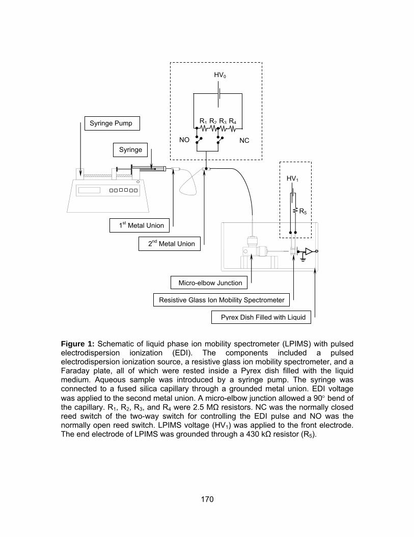
170

Figure 1: Schematic of liquid phase ion mobility spectrometer (LPIMS) with pulsed electrodispersion ionization (EDI). The components included a pulsed electrodispersion ionization source, a resistive glass ion mobility spectrometer, and a Faraday plate, all of which were rested inside a Pyrex dish filled with the liquid medium. Aqueous sample was introduced by a syringe pump. The syringe was connected to a fused silica capillary through a grounded metal union. EDI voltage was applied to the second metal union. A micro-elbow junction allowed a 90° bend of the capillary. R1, R2, R3, and R4 were 2.5 MΩ resistors. NC was the normally closed reed switch of the two-way switch for controlling the EDI pulse and NO was the normally open reed switch. LPIMS voltage (HV1) was applied to the front electrode. The end electrode of LPIMS was grounded through a 430 kΩ resistor (R5).

HV1

R5

Micro-elbow Junction

Resistive Glass Ion Mobility Spectrometer

HV0

R1 R2 R3 R4

NCNO

Syringe Pump

Syringe

1st Metal Union

2nd Metal Union

Pyrex Dish Filled with Liquid

171

Appendix IV

Secondary Electrospray Ionization-Ion Mobility

Spectrometry for Explosive Vapor Detection

Abstract

The unique capability of secondary electrospray ionization (SESI) as a non-

radioactive ionization source to detect analytes in both liquid and gaseous samples

was evaluated using aqueous solutions of three common military explosives: cyclo-

1,3,5-trimethylene-2,4,6-trinitramine (RDX), nitroglycerin (NG) and pentaerythritol

tetranitrate (PETN). The adducts formed between the compounds and their

respective dissociation product, RDX⋅NO2-, NG⋅NO3

- and PETN⋅NO3-, gave the most

intense signal for the individual compound but were more sensitive to temperature

than other species. These auto-adducts were identified as RDX⋅NO2-, NG⋅NO3

- and

PETN⋅NO3- and had maximum signal intensity at 137, 100, and 125°C, respectively.

The reduced mobility values of the three compounds were constant over the

temperature range from 75 °C to 225 °C. The signal-to-noise ratios for RDX, NG and

PETN at 50 mg/L in methanol-water were 340, 270, and 170, respectively, with a

nominal noise of 8±2 pA. In addition to the investigation of auto-adduct formation,

172

the concept of doping the ionization source with non-volatile adduct-forming agents

was investigated and described for the first time. The SESI-IMS detection limit for

RDX was 116 μg/L in the presence of a traditional volatile chloride dopant and 5.30

μg/L in the presence of a non-volatile nitrate dopant. In addition to a lower detection

limit, the nitrate dopant also produced a greater response sensitivity and a higher

limit of linearity than did the traditional volatile chloride dopant.

173

Introduction

Ion mobility spectrometry (IMS) is the established method of choice for the detection

of explosives,1-7 in which radioactive 63Ni ionization source is used to ionize

explosive vapors thermally desorbed from solid particles. A volatile dopant is

frequently employed in 63Ni-IMS to provide a reactant ion.8 The most common

dopant is methylene chloride.3;5;8-16 Other dopants have also been experimented,

including o-dichlorobenzene,3 carbon tetrachloride,4;15 hexachloroethane,6 methyl

chloride,15 trichloromethane,15 chlorobenzene,15 methylene bromide,9;11;16 methyl

bromide,15 methyl iodide9;15 and nitrogen dioxide.10 The use of dopants is also

common in explosives detection by liquid chromatography mass spectrometry (LC-

MS) with electrospray ionization or atmospheric pressure chemical ionization. The

dopant was either added to the LC mobile phase or added post-column. Salts of

ammonium were often used including ammonium acetate17-19, ammonium

formate20;21, ammonium chloride,22;23 and ammonium nitrate23.

The use of a radioactive ionization source such as the 63Ni source in IMS explosive

detection increases the bureaucracy associated with using these detectors in the

field and limits the type of doping agents that can be employed to produce sensitive

and selective reactant ions. Electrospray ionization24 and corona discharge25;26 have

been examined as an alternative non-radioactive ionization source. In this study a

novel non-radioactive ionization source called secondary electrospray ionization

(SESI)27;28 was investigated for the detection of explosives.

174

Secondary electrospray ionization was first introduced by Chen and Hill27 in 1994

when they demonstrated that electrospray ionization (ESI) not only could ionize

solvated analytes, but ESI could also be used to produce reactant ions, from

electrospraying a solvent, to ionize neutral gaseous analytes. Later, Wu et al28

evaluated the analytical figures of merit of SESI, in comparison with ESI, in the

analysis of illicit drugs, and concluded that SESI was a more sensitive ionization

technique than ESI.

The ionization mechanism for SESI is similar to that of atmospheric pressure

chemical ionization, where gas phase reactant ions are produced in the ionization

source and reacted with the sample analyte in the gas-phase forming a charged

analyte, which can then be separated and detected by IMS. In SESI, reactant ions

are produced from the electrospray process. Wu et al28 reported than SESI had

higher ionization efficiency than ESI in the IMS analysis of illicit drug samples.

The primary purposes of this study was to evaluate the unique capability of SESI to

ionize both liquid and gaseous samples using three common military explosives and

to demonstrate the use of non-volatile doping agents for the production of unique

reactant ions. Additionally, this paper investigated the temperature effect on the

stability of the response ions of these explosives, reporting the effect of temperature

on both K0 and sensitivity of the compounds studied.

175


Instrumentation. The SESI-IMS system was constructed at Washington State

University (Figure 1). The SESI-IMS system consisted of a water-cooled ESI source,

a sample introduction unit and an ion mobility spectrometer.

The water-cooled ESI source used in this study has been described in detail by

Clowers et al.29 A voltage of –10 kV was applied to the electrospray needle. The

electrospray solvent was delivered by a Micro-Tech Ultra Plus II MicroLC system

(Micro-Tech Scientific, Vista, CA) at 10 μL/min via a fused silica capillary. Nitrogen

carrier gas flowed at 50 mL/min inside the cooling cavity of the ESI source. In these

studies, the sample was not introduced into the IMS through the electrospray

process as in normal electrospray IMS.

The sample introduction unit was an assembly of a stainless steel Tee tube fitting

(⅛″) and a perforated stainless steel sample inlet ring connected via a Teflon tubing.

The sample, which was pumped at 10 μL/min by a Harvard syringe pump “11”

(Harvard Apparatus, Holliston, MA), entered the Tee tube fitting through a fused

silica capillary (75 μm I.D.) and was carried to the sample inlet ring by nitrogen gas

flowing at 573 ml/min. The sample introduction unit was heated to approximately 210

°C with heating tape. The elevated temperature of the sample introduction unit

ensured that the sample was completely volatilized before entering the ion mobility

176

tube. The sample inlet ring was located between the electrospray needle and the ion

entrance gate. In the ESI-IMS experiments, the explosive compounds were

introduced through the electrospray. In the SESI-IMS experiments, the explosive

compounds were introduced through the sample introduction unit in Figure 1.

The ion mobility spectrometer was made of a stack of stainless steel guard rings (47

mm I.D.), which were connected in series by resistors and insulated from one

another with alumina rings. The drift region was 14.1 cm in length, with a constant

electric field of -379 V/cm, unless stated otherwise. A Bradbury-Nielsen type shutter

gate was used.30 A target screen and an aperture grid were located at the front and

at the end of the ion mobility tube respectively. Nitrogen drift gas flowed at 800

mL/min countercurrent to the direction at which ions were traveling. The temperature

of the IMS housing was varied between 75 and 225 °C. The TNT experiments were

operated at approximately 235 °C.

Signal was detected by a faraday plate, collected and amplified (109 gain) by a

Keithley 427 current amplifier (Keithley Instruments, Cleveland, OH), then processed

by a LabView (National Instruments, Austin, TX) based data acquisition system

written in-house. Spectra were collected at either 25 or 30 ms interval with a pulse

width of 0.2 ms and were averaged 500 times.

The ITEMISER® (Ion Track Instruments, Wilmington, MA), a commercial 63Ni-IMS

instrument, was operated in the explosive mode with purified air as drift gas and

methylene chloride as dopant. 10 μL of 10 mg/L sample solution was pipetted on a

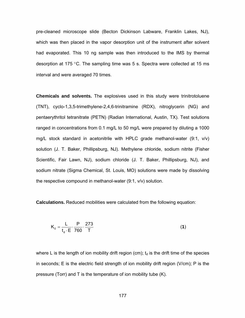
177

pre-cleaned microscope slide (Becton Dickinson Labware, Franklin Lakes, NJ),

which was then placed in the vapor desorption unit of the instrument after solvent

had evaporated. This 10 ng sample was then introduced to the IMS by thermal

desorption at 175 °C. The sampling time was 5 s. Spectra were collected at 15 ms

interval and were averaged 70 times.

Chemicals and solvents. The explosives used in this study were trinitrotoluene

(TNT), cyclo-1,3,5-trimethylene-2,4,6-trinitramine (RDX), nitroglycerin (NG) and

pentaerythritol tetranitrate (PETN) (Radian International, Austin, TX). Test solutions

ranged in concentrations from 0.1 mg/L to 50 mg/L were prepared by diluting a 1000

mg/L stock standard in acetonitrile with HPLC grade methanol-water (9:1, v/v)

solution (J. T. Baker, Phillipsburg, NJ). Methylene chloride, sodium nitrite (Fisher

Scientific, Fair Lawn, NJ), sodium chloride (J. T. Baker, Phillipsburg, NJ), and

sodium nitrate (Sigma Chemical, St. Louis, MO) solutions were made by dissolving

the respective compound in methanol-water (9:1, v/v) solution.

Calculations. Reduced mobilities were calculated from the following equation:

0d

L P 273Kt E 760 T

= ⋅ ⋅⋅

(1)

where L is the length of ion mobility drift region (cm); td is the drift time of the species

in seconds; E is the electric field strength of ion mobility drift region (V/cm); P is the

pressure (Torr) and T is the temperature of ion mobility tube (K).

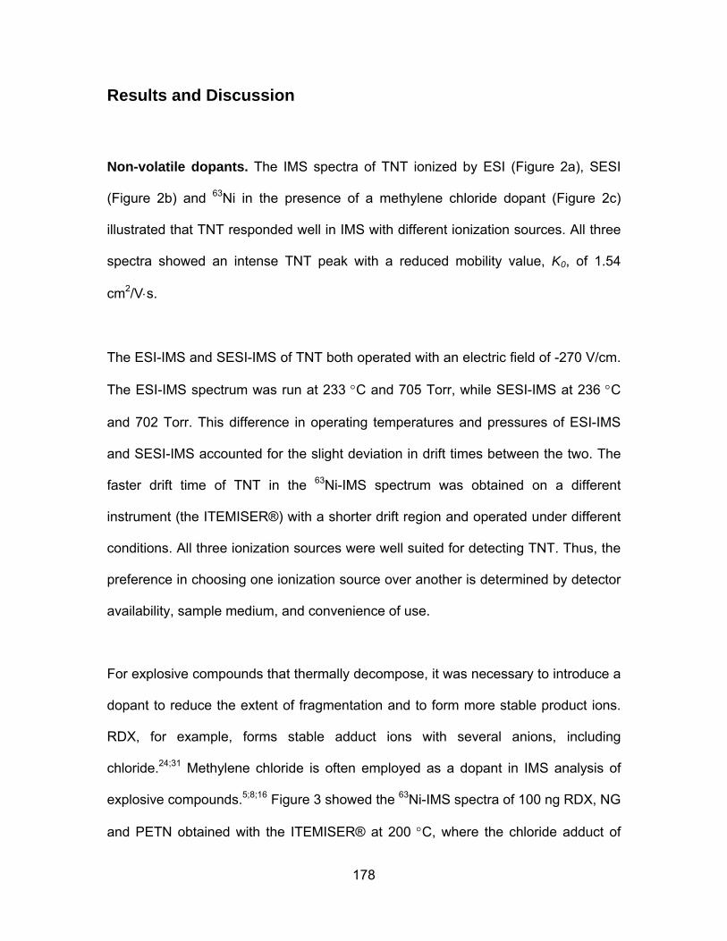
178


Non-volatile dopants. The IMS spectra of TNT ionized by ESI (Figure 2a), SESI

(Figure 2b) and 63Ni in the presence of a methylene chloride dopant (Figure 2c)

illustrated that TNT responded well in IMS with different ionization sources. All three

spectra showed an intense TNT peak with a reduced mobility value, K0, of 1.54

cm2/V⋅s.

The ESI-IMS and SESI-IMS of TNT both operated with an electric field of -270 V/cm.

The ESI-IMS spectrum was run at 233 °C and 705 Torr, while SESI-IMS at 236 °C

and 702 Torr. This difference in operating temperatures and pressures of ESI-IMS

and SESI-IMS accounted for the slight deviation in drift times between the two. The

faster drift time of TNT in the 63Ni-IMS spectrum was obtained on a different

instrument (the ITEMISER®) with a shorter drift region and operated under different

conditions. All three ionization sources were well suited for detecting TNT. Thus, the

preference in choosing one ionization source over another is determined by detector

availability, sample medium, and convenience of use.

For explosive compounds that thermally decompose, it was necessary to introduce a

dopant to reduce the extent of fragmentation and to form more stable product ions.

RDX, for example, forms stable adduct ions with several anions, including

chloride.24;31 Methylene chloride is often employed as a dopant in IMS analysis of

explosive compounds.5;8;16 Figure 3 showed the 63Ni-IMS spectra of 100 ng RDX, NG

and PETN obtained with the ITEMISER® at 200 °C, where the chloride adduct of

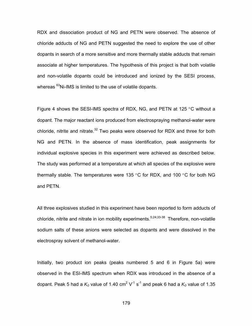
179

RDX and dissociation product of NG and PETN were observed. The absence of

chloride adducts of NG and PETN suggested the need to explore the use of other

dopants in search of a more sensitive and more thermally stable adducts that remain

associate at higher temperatures. The hypothesis of this project is that both volatile

and non-volatile dopants could be introduced and ionized by the SESI process,

whereas 63Ni-IMS is limited to the use of volatile dopants.

Figure 4 shows the SESI-IMS spectra of RDX, NG, and PETN at 125 °C without a

dopant. The major reactant ions produced from electrospraying methanol-water were

chloride, nitrite and nitrate.32 Two peaks were observed for RDX and three for both

NG and PETN. In the absence of mass identification, peak assignments for

individual explosive species in this experiment were achieved as described below.

The study was performed at a temperature at which all species of the explosive were

thermally stable. The temperatures were 135 °C for RDX, and 100 °C for both NG

and PETN.

All three explosives studied in this experiment have been reported to form adducts of

chloride, nitrite and nitrate in ion mobility experiments.5;24;33-38 Therefore, non-volatile

sodium salts of these anions were selected as dopants and were dissolved in the

electrospray solvent of methanol-water.

Initially, two product ion peaks (peaks numbered 5 and 6 in Figure 5a) were

observed in the ESI-IMS spectrum when RDX was introduced in the absence of a

dopant. Peak 5 had a K0 value of 1.40 cm2 V-1 s-1 and peak 6 had a K0 value of 1.35

180

cm2/V⋅s. Peaks 2 and 3, in all of the spectra in Figure 5, corresponded to nitrite and

nitrate ions respectively. Figure 5b is the resulting spectrum when RDX was

electrosprayed in presence of nitrite dopant. Compared with Figure 1a, the signal

intensity of peak 5 increased; Similarly, RDX was electrosprayed in the presence of

nitrate dopant, the signal intensity of peak 6 increased (Figure 5c); When RDX was

electrosprayed in the presence of chloride dopant, a third peak – peak 4, with a K0

value of 1.44 cm2/V⋅s appeared (Figure 5d). The increase in intensity of specific

peaks in different dopant environment suggested that the three peaks of RDX were

M⋅Cl- (K0 1.44), M⋅NO2- (K0 1.40) and M⋅NO3

- (K0 1.35).

Peak assignments for NG and PETN were performed in the same manner, with the

exception of (M-H)- of NG and of PETN, by observing the increased intensity in

different analyte peaks in presence of different dopant additives. The (M-H)- species

of NG and PETN were assigned based on comparison with literature data. Peak

assignments for species of the three explosive compounds are tabulated along with

their respective literature values in Table 1.

The non-volatile dopant studies were repeated with SESI-IMS. The SESI-IMS

spectra of RDX in the absence of any dopant and in the presence of the added

dopants (Figure 5e-h) showed that RDX peaks were more intense when ionized by

SESI than by ESI. It was interesting to note that while reactant ions were present in

the ESI-IMS spectra, no reactant ions of considerable intensity were observed in the

SESI-IMS spectra of RDX. The only difference between the ESI-IMS and SESI-IMS

experiments was the sample introduction method. In ESI-IMS, the analyte was

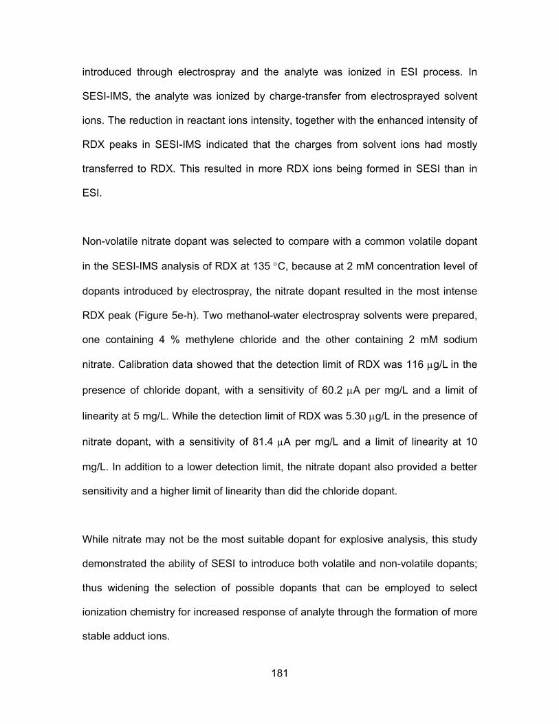
181

introduced through electrospray and the analyte was ionized in ESI process. In

SESI-IMS, the analyte was ionized by charge-transfer from electrosprayed solvent

ions. The reduction in reactant ions intensity, together with the enhanced intensity of

RDX peaks in SESI-IMS indicated that the charges from solvent ions had mostly

transferred to RDX. This resulted in more RDX ions being formed in SESI than in

ESI.

Non-volatile nitrate dopant was selected to compare with a common volatile dopant

in the SESI-IMS analysis of RDX at 135 °C, because at 2 mM concentration level of

dopants introduced by electrospray, the nitrate dopant resulted in the most intense

RDX peak (Figure 5e-h). Two methanol-water electrospray solvents were prepared,

one containing 4 % methylene chloride and the other containing 2 mM sodium

nitrate. Calibration data showed that the detection limit of RDX was 116 μg/L in the

presence of chloride dopant, with a sensitivity of 60.2 μA per mg/L and a limit of

linearity at 5 mg/L. While the detection limit of RDX was 5.30 μg/L in the presence of

nitrate dopant, with a sensitivity of 81.4 μA per mg/L and a limit of linearity at 10

mg/L. In addition to a lower detection limit, the nitrate dopant also provided a better

sensitivity and a higher limit of linearity than did the chloride dopant.

While nitrate may not be the most suitable dopant for explosive analysis, this study

demonstrated the ability of SESI to introduce both volatile and non-volatile dopants;

thus widening the selection of possible dopants that can be employed to select

ionization chemistry for increased response of analyte through the formation of more

stable adduct ions.

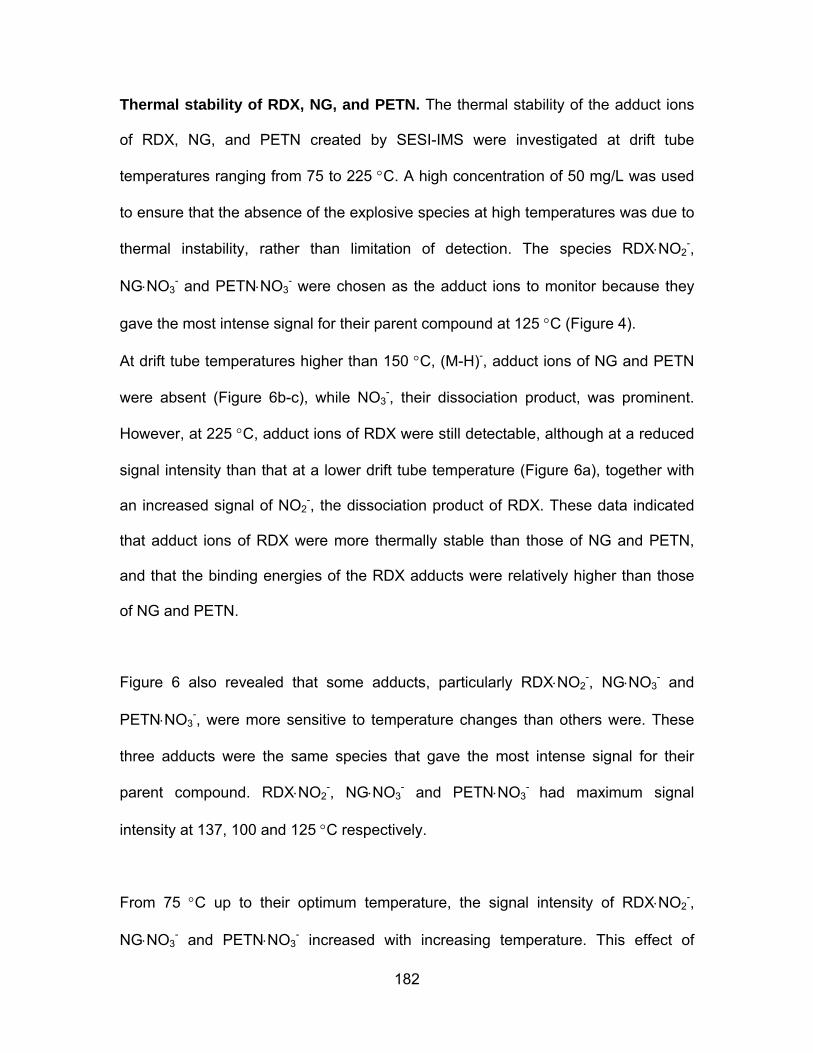
182

Thermal stability of RDX, NG, and PETN. The thermal stability of the adduct ions

of RDX, NG, and PETN created by SESI-IMS were investigated at drift tube

temperatures ranging from 75 to 225 °C. A high concentration of 50 mg/L was used

to ensure that the absence of the explosive species at high temperatures was due to

thermal instability, rather than limitation of detection. The species RDX⋅NO2-,

NG⋅NO3- and PETN⋅NO3

- were chosen as the adduct ions to monitor because they

gave the most intense signal for their parent compound at 125 °C (Figure 4).

At drift tube temperatures higher than 150 °C, (M-H)-, adduct ions of NG and PETN

were absent (Figure 6b-c), while NO3-, their dissociation product, was prominent.

However, at 225 °C, adduct ions of RDX were still detectable, although at a reduced

signal intensity than that at a lower drift tube temperature (Figure 6a), together with

an increased signal of NO2-, the dissociation product of RDX. These data indicated

that adduct ions of RDX were more thermally stable than those of NG and PETN,

and that the binding energies of the RDX adducts were relatively higher than those

of NG and PETN.

Figure 6 also revealed that some adducts, particularly RDX⋅NO2-, NG⋅NO3

- and

PETN⋅NO3-, were more sensitive to temperature changes than others were. These

three adducts were the same species that gave the most intense signal for their

parent compound. RDX⋅NO2-, NG⋅NO3

- and PETN⋅NO3- had maximum signal

intensity at 137, 100 and 125 °C respectively.

From 75 °C up to their optimum temperature, the signal intensity of RDX⋅NO2-,

NG⋅NO3- and PETN⋅NO3

- increased with increasing temperature. This effect of

183

temperature on response indicated the mechanism of adduct formation. Apparently,

RDX⋅NO2-, NG⋅NO3

- and PETN⋅NO3- were adducts formed between the compound

and its decomposition product ion. Since RDX dissociated to NO2-, NG and PETN

dissociated to NO3-, the nitrite and nitrate adduct ions originated from the

dissociation products of their respective compound. This involved two steps: (1) the

molecular ion dissociated to form nitrite or nitrate and (2) the molecule reacted with

the dissociated nitrite or nitrate thus forming an autoionization product.

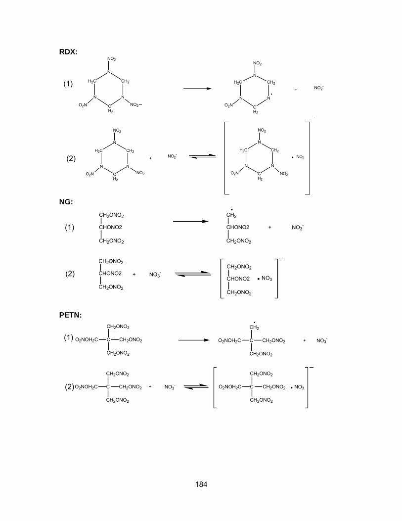
184

RDX:

H2C

N

CH2

N

CH2

N

NO2

NO2

O2N

H2C

N

CH2

N

CH2

N

NO2

O2N

NO2-

+

H2C

N

CH2

N

CH2

N

NO2

NO2

O2N

NO2-

H2C

N

CH2

N

CH2

N

NO2

NO2

O2N

. NO2+

NG:

CHONO2

CH2ONO2

CH2ONO2

CHONO2

CH2ONO2

CH2ONO2

NO3-

CHONO2

CH2

CH2ONO2

CHONO2

CH2ONO2

CH2ONO2

. NO3

NO3-+

+

PETN:

C CH2ONO2

CH2ONO2

CH2ONO2

O2NOH2C

C CH2ONO2

CH2ONO2

CH2ONO2

O2NOH2C NO3-

C CH2ONO2

CH2

CH2ONO2

O2NOH2C

C CH2ONO2

CH2ONO2

CH2ONO2

O2NOH2C . NO3

NO3-+

+

(1)

(2)

(1)

(2)

(1)

(2)

185

Above their optimum temperatures, the signal intensity of RDX⋅NO2-, NG⋅NO3

- and

PETN⋅NO3- decreased with increasing temperature. This decrease in signal intensity

can be attributed to the thermal decomposition of the autoionization products and/or

the advance decomposition of the compound itself into NO2- or NO3

-, as evidenced

by the presence of NO2- for RDX and NO3

- for NG and PETN at high temperatures.

Temperature effect on K0. The reduced mobility values of the molecular ions and

the various adduct ions of RDX, NG and PETN were plotted versus the drift tube

temperature used in this study, from 75 to 225 °C (Figure 7). Error bars were omitted

from the plot because they were smaller in size than the K0 markers. The average

standard deviation for the K0 values was 0.001 cm2/V⋅s, with a maximum standard

deviation of 0.002 cm2/V⋅s. The K0 values of the various explosive species showed a

slight negative dependence on temperature, with the K0 value decreasing by 2% at

most over the temperature range. In conclusion, the K0 values of the explosive

species appeared to be constant (< ± 2%) over a 150 °C temperature range where

SESI-IMS is used.

Signal to Noise Ratio. With 50 ng/μL of liquid sample entering the sample

introduction unit at 10 μL/min, being volatilized at a temperature of 210 °C and

carried by nitrogen gas flowing at 940 mL/min, a 50 ng/μL liquid sample was,

therefore, equivalent to 0.53 mg m-3 or 102 ppbv of RDX, 101 ppbv of NG and 72

ppbv of PETN in nitrogen.

186

In the SESI-IMS experiments, in the absence of added dopant, the signal-to-noise

ratios for 50 mg/L or 0.53 mg/m3 of RDX (137 °C), NG (100 °C) and PETN (125 °C)

were 340, 270 and 170, respectively with a nominal noise of 8 ± 2 pA. At this level of

signal-to-noise ratio measured, the sensitivity of the SESI-IMS system was sufficient

to detect explosives in workplace air samples, where the maximum airborne

concentration of explosives recommended by the American Conference of

Governmental Industrial Hygienists (1986) to be 0.5 mg m-3 for NG and 1.5 mg/m3

for RDX.

Conclusions

SESI is a non-radioactive ionization source, which can be used to detect both vapor

phase and aqueous phase explosives. Non-volatile dopants can be used with SESI

to enhance both sensitivity and selectivity. Data showed that SESI-IMS analysis of

RDX, in the presence of a non-volatile nitrate dopant, produced not only a lower

detection limit, but also a greater response sensitivity and a higher limit of linearity,

than in the presence of a common volatile chloride dopant.

Acknowledgement

The authors thank GE Ion Track (Wilmington, MA) for providing the ITEMISER®

instrument and partial support for the investigation.

187

References

(1) Karasek, K. W.; Denney, D. W. Journal of Chromatography 1974, 93, 141-147.

(2) Karasek, K. W. Research/Development 1974, 25, 32-36.

(3) Spangler, G. E.; Lawless, P. A. Analytical Chemistry 1978, 50, 884-92.

(4) Spangler, G. E.; Carrico, J. P.; Campbell, D. N. Journal of Testing and Evaluation 1985, 13, 234-40.

(5) Lawrence, A. H.; Neudorfl, P. Analytical Chemistry 1988, 60, 104-09.

(6) Fetterolf, D. D.; Clark, T. D. Journal of Forensic Sciences 1993, 38, 28-39.

(7) Ewing, R. G.; Miller, C. J. Field Analytical Chemistry and Technology 2001, 5, 215-21.

(8) Lawrence, A. H.; Neudorfl, P.; Stone, J. A. International Journal of Mass Spectrometry 2001, 209, 185-95.

(9) Proctor, C. J.; Todd, J. F. J. Analytical Chemistry 1984, 56, 1794-97.

(10) Davies, J. P.; Blackwood, L. G.; Davis, S. G.; Goodrich, L. D.; Larson, R. A. Analytical Chemistry 1993, 65, 3004-09.

(11) Brittain, A. H.; Brokenshire, J. L. Proceeding of the Fifth International Workshop on Ion Mobility Spectrometry, Jackson, Wyoming, 1996.

(12) Atkinson, D. A.; Crockett, A. B.; Jenkins, T. F. Proceeding of the Fifth International Workshop on Ion Mobility Spectrometry, Jackson, Wyoming, 1996.

(13) Eiceman, G. A.; Preston, D.; Tiano, G.; Rodriguez, J.; Parmeter, J. E. Talanta 1997, 45, 57-74.

(14) Munro, W. A. ; Thomas, C. L. P.; Langford, M. L. Analytica Chimica Acta 1998, 375, 49-63.

(15) Daum, K. A.; Atkinson, D. A.; Ewing, R. G. Talanta 2001, 55, 491-500.

(16) Daum, K. A.; Atkinson, D. A.; Ewing, R. G.; Knighton, W. B.; Grimsrud, E. P. Talanta 2001, 54, 299-306.

(17) Wu, Z.; Hendrickson, C. L.; Rodgers, R. P.; Marshall, A. G. Analytical Chemistry 2002, 74, 1879-1883.

188

(18) Schreiber, A.; Efer, J.; Engewald, W. Journal of Chromatography A 2000, 869, 411-25.

(19) Casetta, B.; Garofolo, F. Organic Mass Spectrometry 1994, 29, 517-25.

(20) Cassada, D. A.; Monson, S. J.; Snow, D. D.; Spalding, R. F. Journal of Chromatography A 1999, 844, 87-95.

(21) Gapeev, A.; Sigman, M.; Yinon, J. Rapid Communications in Mass Spectrometry 2003, 17, 943-48.

(22) Evans, C. S. ; Sleeman, R.; Luke, J.; Keely, B. J. Rapid Communications in Mass Spectrometry 2002, 16, 1883-91.

(23) Zhao, X.; Yinon, J. Journal of Chromatography A 2002, 977, 59-68.

(24) Asbury, G. R.; Klasmeier, J.; Hill, H. H. Jr. Talanta 2000, 50, 1291-98.

(25) Tabrizchi, M.; Abedi, A. International Journal of Mass Spectrometry 2002, 218, 75-85.

(26) Khayamian, T.; Tabrizchi, M.; Jafari, M. T. Talanta 2003, 59, 327-33.

(27) Chen, Y. H.; Hill, H. H. Jr. Journal of Microcolumn Separations 1994, 6, 515-24.

(28) Wu, C.; Siems, W. F.; Hill, H. H. Jr. Analytical Chemistry 2000, 72, 396-403.

(29) Clowers, B. H.; Steiner, W. S.; Dion, H. M.; Matz, L. M.; Tam, M.; Tarver, E. E.; Hill, H. H. Jr. Field Analytical Chemistry and Technology 2001, 5, 302-12.

(30) Bradbury, N. E.; Nielson, R. A. Phys. Rev. 1936, 49, 388-393.

(31) Rodriguez, J. E. Atmospheric Pressure Chemical Ionization of Nitro-Containing Organic Explosives and Other Nitro-Organic Compounds in Mass Spectrometry and Ion Mobility Spectrometry, Masters Thesis, New Mexico State University: Las Cruces, NM, 1996.

(32) Asbury, G. R.; Hill, H. H. Jr. International Journal for Ion Mobility Spectrometry 1999, 2, 1-8.

(33) Ritchie, R. K.; Kuja, F. J.; Jackson, R. A.; Loveless, A. J.; Danylewych-May, L. L. Proceedings of the Substance Detection Systems, Bellingham, WA, 1994.

(34) Fetterolf, D. D. In Advances in Analysis and Detection of Explosives; edited by J. Yinon; Kluwer Academic Publishers: Dordrecht, 1993; pp. 117-131.

(35) Huang, S. D.; Kolaitis, L.; Lubman, D. M. Applied Spectroscopy 1987, 41, 1371-76.

(36) Spangler, G. E.; Carrico, J. P.; Kim, S. H. Proceedings of the International Symposium on Analysis and Detection of Explosive, Quantico, VA, 1983.

189

(37) Wernlund, R. F.; Cohen, M. J.; Kindel, R. C. Proceedings of the New Concept Symposium and Workshop on Detection and Identification of Explosives, Reston, VA, 1978.

(38) Danylewych-May, L. L. Proceedings of the First International Symposium on Explosive Detection Technology, Atlantic City, NJ, 1991.

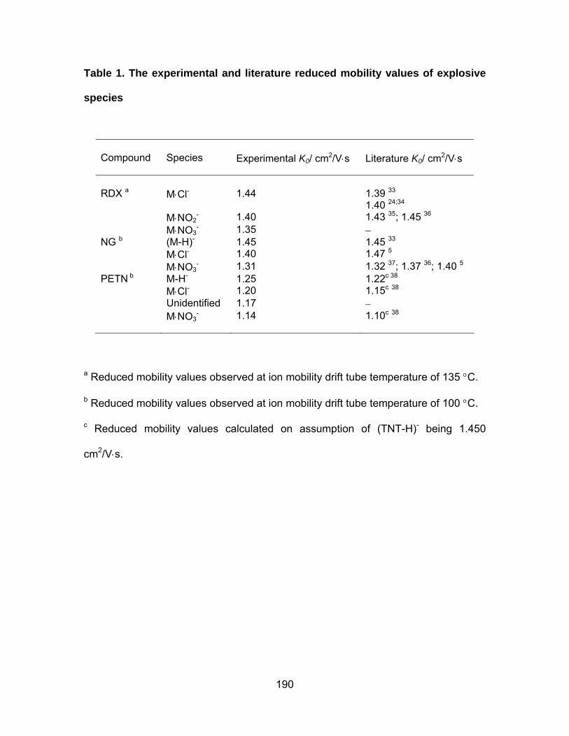
190

Table 1. The experimental and literature reduced mobility values of explosive

species

Compound

Species

Experimental K0/ cm2/V⋅s

Literature K0/ cm2/V⋅s

RDX a

M⋅Cl-

1.44

1.39 33 1.40 24;34

M⋅NO2- 1.40 1.43 35; 1.45 36

M⋅NO3- 1.35 −

NG b (M-H)- 1.45 1.45 33 M⋅Cl- 1.40 1.47 5 M⋅NO3

- 1.31 1.32 37; 1.37 36; 1.40 5 PETN b M-H- 1.25 1.22c 38 M⋅Cl- 1.20 1.15c 38 Unidentified 1.17 − M⋅NO3

- 1.14

1.10c 38

a Reduced mobility values observed at ion mobility drift tube temperature of 135 °C.

b Reduced mobility values observed at ion mobility drift tube temperature of 100 °C.

c Reduced mobility values calculated on assumption of (TNT-H)- being 1.450

cm2/V⋅s.

191

FIGURE CAPTIONS

Figure 1. Schematic of secondary electrospray ionization-ion mobility spectrometer.

Figure 2. (a) ESI-IMS spectrum of 10 mg L-1 TNT; (b) SESI-IMS spectrum of 10 mg

L-1 TNT; (c) 63Ni-IMS spectrum of 100ng TNT with methylene chloride as dopant.

Figure 3. 63Ni-IMS spectra of 100ng of (a) RDX (b) NG and (c) PETN. Spectra were

obtained at 200 °C with methylene chloride as dopant.

Figure 4. SESI-IMS spectra of 50 mg L-1 (a) RDX (b) NG and (c) PETN in methanol-

water. All spectra were run at 125 °C.

Figure 5. Effect of non-volatile dopants: ESI-IMS spectra of 50 mg L-1 RDX in (a)

methanol-water (b) 2 mM NaNO2 (c) 2 mM NaNO3 (d) 2 mM NaCl. SESI-IMS

spectra of 50 mg L-1 RDX in methanol-water with electrospraying (e) methanol-water

(f) 1.45 mM NaNO2 (g) 2 mM NaNO3 (h) 2mM NaCl. All spectra were run at 135 °C.

Peak assignments: (1) Cl- (2) NO2- (3) NO3

- (4) RDX⋅Cl- (5) RDX⋅NO2- (6) RDX⋅NO3

-

Figure 6. Thermal stability of RDX, NG and PETN species: Plots of SESI-IMS signal

intensity versus drift tube temperature of (a) RDX (b) NG and (c) PETN.

Figure 7. Plot of SESI-IMS reduced mobilities of RDX, NG and PETN species

versus drift tube temperature. Average standard deviation for the K0 values was

192

0.001 cm2 V-1 s-1, with maximum standard deviation at 0.002 cm2 V-1 s-1. Error bars

were omitted from the plot because they were smaller in size than the data point

markers.

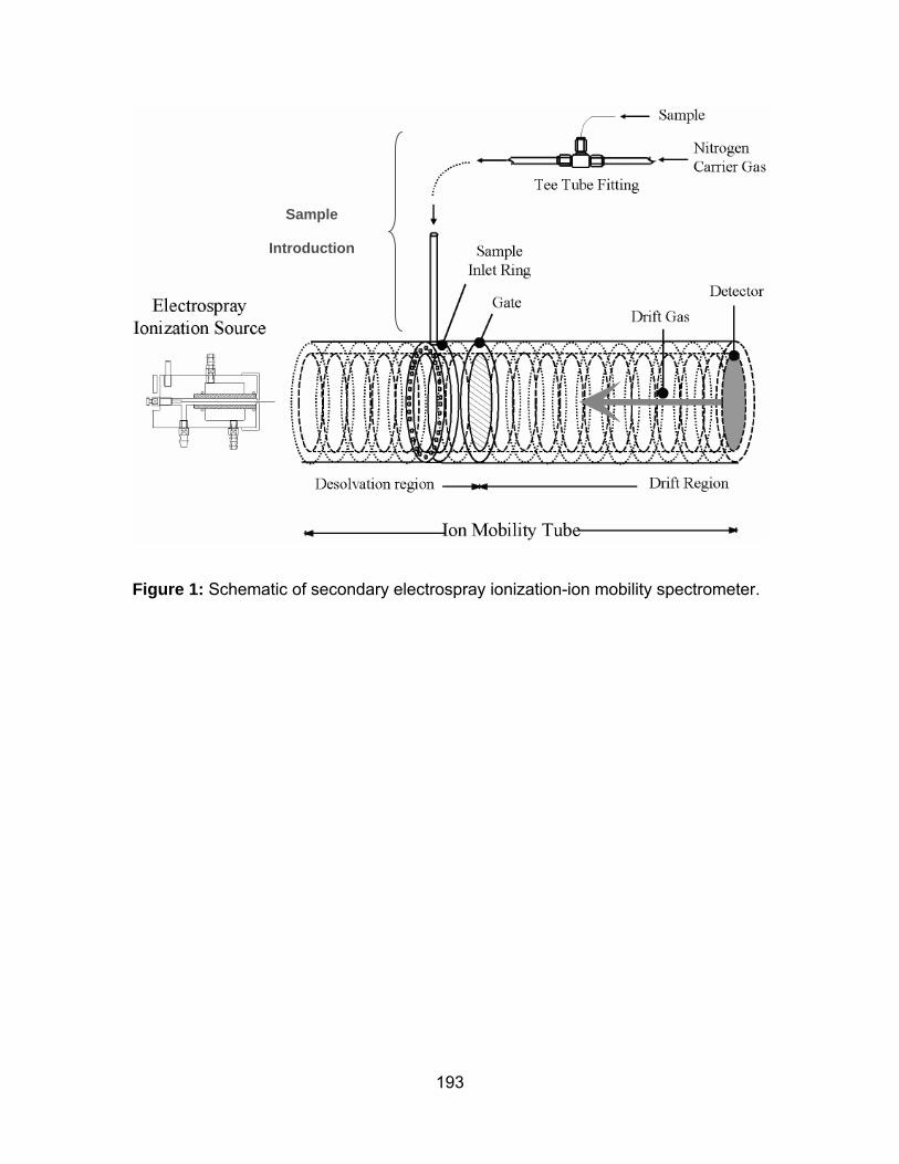
193

Figure 1: Schematic of secondary electrospray ionization-ion mobility spectrometer.

Sample

Introduction

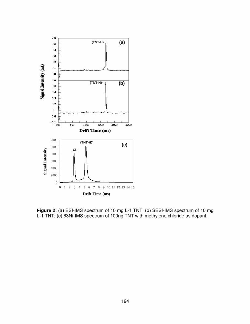
194

0

2000

4000

6000

8000

10000

12000

0 1 2 3 4 5 6 7 8 9 10 11 12 13 14 15

Drift Time (ms)

Sign

al In

tens

ity

Figure 2: (a) ESI-IMS spectrum of 10 mg L-1 TNT; (b) SESI-IMS spectrum of 10 mg L-1 TNT; (c) 63Ni-IMS spectrum of 100ng TNT with methylene chloride as dopant.

(TNT-H)-

(b)

(a)

(TNT-H)-

Cl-

(TNT-H)-

(c)

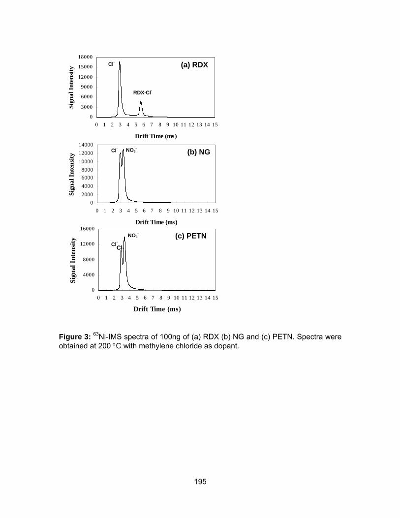
195

Figure 3: 63Ni-IMS spectra of 100ng of (a) RDX (b) NG and (c) PETN. Spectra were obtained at 200 °C with methylene chloride as dopant.

0

3000

6000

9000

12000

15000

18000

0 1 2 3 4 5 6 7 8 9 10 11 12 13 14 15

Drift Time (ms)

Sign

al In

tens

ity

0

4000

8000

12000

16000

0 1 2 3 4 5 6 7 8 9 10 11 12 13 14 15

Drift Time (ms)

Sign

al In

tens

ity

02000400060008000

100001200014000

0 1 2 3 4 5 6 7 8 9 10 11 12 13 14 15

Drift Time (ms)

Sign

al In

tens

ity

Cl-

(a) RDX

(b) NG

(c) PETN

Cl-

Cl- NO3-

NO3-

RDX·Cl-

Cl-

196

Figure 4: SESI-IMS spectra of 50 mg L-1 (a) RDX (b) NG and (c) PETN in methanol-water. All spectra were run at 125 °C.

(a) RDX

(b) NG

(c) PETN

M·NO3-

M·NO2-

M·Cl-

M·NO3-

NO3-

M·NO3-

M·NO2-

NO3-

M·Cl-

(M-H)-

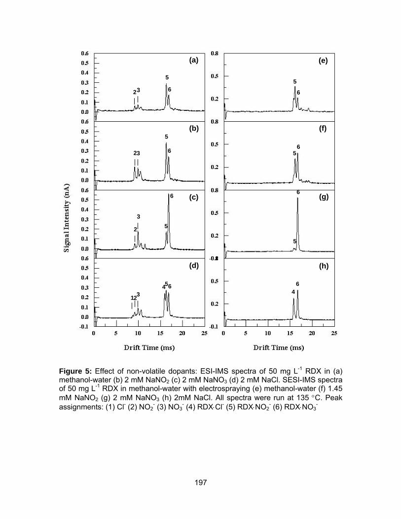
197

Figure 5: Effect of non-volatile dopants: ESI-IMS spectra of 50 mg L-1 RDX in (a) methanol-water (b) 2 mM NaNO2 (c) 2 mM NaNO3 (d) 2 mM NaCl. SESI-IMS spectra of 50 mg L-1 RDX in methanol-water with electrospraying (e) methanol-water (f) 1.45 mM NaNO2 (g) 2 mM NaNO3 (h) 2mM NaCl. All spectra were run at 135 °C. Peak assignments: (1) Cl- (2) NO2

- (3) NO3- (4) RDX⋅Cl- (5) RDX⋅NO2

- (6) RDX⋅NO3-

(a)

(b)

(c)

(d) (h)

(g)

(f)

(e)

1 2 3 4

5

5

5

5

4 6 5

6

6

6

6

6

5

6

5

2

3

2 3

2 3

6

198

0

0.1

0.2

0.3

0.4

0.5

0.6

0.7

50 75 100 125 150 175 200 225 250Temperature (Celsius)

Sign

al In

tens

ity (n

A)

0.0

0.1

0.2

0.3

0.4

0.5

0.6


Sign

al In

tens

ity (n

A)

0.0

0.1

0.2

0.3

0.4


Sign

al In

tens

ity (n

A)

Figure 6: Thermal stability of RDX, NG, and PETN species: Plots of SESI-IMS signal intensity versus drift tube temperature of (a) RDX (b) NG and (c) PETN.

(a) RDX

(b) NG

(c) PETN

M·NO2-

K0 1.17

M·NO3-

M·NO3-

M·Cl-

(M-H)-

M·NO3-

(M-H)-

M·Cl-

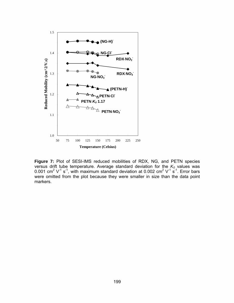
199

1.0

1.1

1.2

1.3

1.4

1.5

50 75 100 125 150 175 200 225 250

Temperature (Celsius)

Red

uced

Mob

ility

(cm

^2/V

.s)

Figure 7: Plot of SESI-IMS reduced mobilities of RDX, NG, and PETN species versus drift tube temperature. Average standard deviation for the K0 values was 0.001 cm2 V-1 s-1, with maximum standard deviation at 0.002 cm2 V-1 s-1. Error bars were omitted from the plot because they were smaller in size than the data point markers.

NG⋅Cl-

(NG-H)-

PETN⋅NO3-

PETN K0 1.17

(PETN-H)-

NG⋅NO3-

RDX⋅NO2-

RDX⋅NO3-

PETN⋅Cl-

liquid phase ion mobility spectrometry - … · throughout my student life: ... liquid phase ion...

Documents