5.8 Liquid-Liquid phase diagrams

Key points 1.  Phase separation of partially miscible liquids

may occur when T is below UCST or above LCST

2.  UCST is the highest T at which phase separation occurs. LCST is the lowest T at which phase separation occurs

3.  The outcome of a distillation of a low-boiling azeotrope depends on whether the liquids become fully miscible before they boil or boiling occurs occurs before mixing is complete

4.  Consider partially miscible liquids

(a) Phase separation •  Suppose a small amount of liquid B is

added to a sample of another liquid B at T’. Liquid B dissolves completely forming a single phase

•  As more B is added, a stage comes at which no more dissolves. The sample consists of two phases in equilibrium; A-rich phase (a’’) and B-rich phase (a’)

•  Lever rule is still applied •  As more B is added, a stage comes at

so much B is present and it can dissolve all the A forming a single phase

5.8 Liquid-Liquid phase diagrams

(b) Critical solution temperature •  Upper critical solution temperature

(UCST) : the highest temperature at which phase separation occurs

•  The phase boundary: ∂∆mixG/∂x = 0

•  Lower critical solution temperature (LCST) : below LCST they mix in all proportions and above which they form two phases

•  Some systems have both upper and lower critical solution temperatures (Figure 5.47)

5.8 Liquid-Liquid phase diagrams

ln x1− x

+ξ 1− 2x( ) = 0

(c) The distillation of partially miscible liquids •  Consider a pair of liquids that are

partially miscible and form a low-boiling azeotrope

•  This combination is quite common because both properties reflect the tendency of A and B to avoid each other

•  (1) The liquids become fully miscible before they boil and (2) the boiling occurs before mixing is complete

•  Distillation of a1 leads to a vapor of composition b1

•  b1 condenses to the completely miscible single-phase solution at b2

•  When this distillate is cooled to b3, phase-separation occurs

5.8 Liquid-Liquid phase diagrams

(c) The distillation of partially miscible liquids •  Distillate obtained from a liquid of

composition of a1 has composition b3 •  The distillate is a two-phase mixture

of b3’ and b3’’ •  A system at e1 forms two phases,

which persist up to the boiling point at e2. The vapor of this mixture has the same composition as liquids (azeotrope)

•  Condensing a vapor of composition e3 gives a two-phase liquid of the same overall composition

5.8 Liquid-Liquid phase diagrams

5.9 Liquid-solid phase diagrams

Key points 1.  At the eutectic composition the liquid phase

solidifies without change of composition 2.  The phase equilibria of binary systems in which

the components react may also be summarized by a phase diagram

3.  In some cases, a solid compound does not survive melting

(a) Eutectics •  a1 → a2 : The system enters the two-phase

region labeled ‘Liquid+B’. Pure solution begins to come out of solution and remaining liquid becomes richer in A

•  a2 → a3 : More of the solid B forms •  a3 → a4 : At the end of this step, there is less

liquid a3, and its composition is given by e2. This liquid now freeze to give a two-phase system of pure B and pure A

•  The isopleth e2 corresponds to “the eutectic composition”: a liquid with the eutectic composition freezes at a single temperature, without previously depositing solid A or B

•  Thermal analysis is a powerful way of detecting eutectics

•  Eutectic halt

5.9 Liquid-solid phase diagrams

(b) Reacting systems •  Many binary mixtures react to produce

compounds •  For example, Ga + As ⇌ GaAs •  Although three constituents are present,

there are only two components •  Consider A + B ⇌ C •  Consider a system prepared by mixing an

excess of B with A that consists of C and unreacted B

•  The solid deposited on cooling along the isopleth a is C

•  Below a4 there are two solid phases: solid B and solid C phases

•  The pure compound C melts congruently, that is the composition of the liquid it forms is the same as that of the solid

5.9 Liquid-solid phase diagrams

(c) Incongruent melting

•  b1 → b2 : Solid solution rich in Na begins to deposit •  b2 → b3 : A solid solution rich in Na deposits, but a reaction occurs

to form Na2K •  b3 : Three phases are in mutual equilibrium; liquid + Na2K + a solid

solution rich in Na (peritectic line) •  b3 → b4 : The amount of solid compound increases until at b4 the

liquid reaches its eutectic composition. It solidifies to give a two-phase solid of a solid solution rich in K and solid Na2K

5.9 Liquid-solid phase diagrams

• C is not stable as a liquid (Liquid Na2K is unstable) • a1 → a2 : A solid solution rich in Na is deposited • a2 → just below a3 : The sample is entirely solid and consists of a solid solution rich in Na and solid Na2K

5.10 The solvent activity

Key points 1.  The activity is an effective concentration that

preserves the form of the expression for the chemical potential

•  The general form of the chemical potential of a real or ideal solvent is given by a straightforward modification of µA = µA* + RTln(pA/pA*)

•  For an ideal solution, the solvent obeys Raoult’s law and µA = µA* + RTln(xA)

•  The form of this relation can be preserved when the solution does not obey Raoult’s law

•  The quantity aA is the activity of A (an “effective” mole fraction) •  The activity coefficient, ϒ

5.10 The solvent activity

µA = µA∗ + RT lnaA aA =

pAp∗A

aA = γAxA and γA →1 as xA →1

µA =µA∗ +RTlnxA +RTln γA

5.11 The solute activity

Key points 1.  The chemical potential of a solute in an ideal-

dilute solution is defined on the basis of Henry’s law

2.  The activity of a solute takes into account departures from Henry’s law behavior

3.  An alternative approach to the definition of the solute activity is based on the molality of the solute

4.  The biological standard state of a species in solution is defined as pH = 7 (and 1 bar)

•  A solute B that satisfies Henry’s law has a vapor pressure pB = KBxB

•  KB and pB* are characteristics of solute

•  If the solution is ideal, KB = pB* and

5.11 The solute activity (a) Ideal-dilute solutions

µB = µB∗ + RT ln pB

p∗B= µB

∗ + RT ln KB

p∗B+ RT ln xB

µΘB = µB

∗ + RT ln KB

pB∗

µB =µΘ +RTlnxB

µΘB =µB

∗

•  We now permit deviations from ideal-dilute, Henry’s law behavior

•  An activity coefficient : all the deviations from ideality are captured in the activity coefficient ϒB.

5.11 The solute activity (b) Real solutes

µB = µΘ + RT lnaB aB =

pBK B

aB = γBxBaB → xB and γB →1 as xB → 0

•  The selection of a standard state is entirely arbitrary •  In chemistry, compositions are often expressed as molalities, b, in

place of mole fractions

•  We incorporate the deviations from ideality by introducing an

activity and a dimensionless activity coefficient

5.11 The solute activity (c) Activities in terms of molalities

µB =µBΘ +RTlnbB

aB = γBbB

bΘ where γB →1 as bB → 0

µ = µΘ + RT lna

•  The conventional standard state of hydrogen ions : unit activity corresponding to pH = 0

•  In biochemistry, it is common to adopt the biological standard state, in which pH = 7

•  G⊕, H⊕, µ⊕, and S⊕ for the biological standard state

•  7RTln10 = 39.96 kJ/mol. The two standard values differ by about 40 kJ/mol

5.11 The solute activity (d) The biological standard state

µ H+( ) = µΘ H+( )+ RT lna H+( ) = µΘ H+( )− RT ln10( )× pHµ⊕ H+( ) = µΘ H+( )− 7RT ln10

5.12 The activities of regular solutions

Key points 1.  The Margules equations relate the activities of

the components of a model regular solution to its composition

2.  The Margules equations lead to expressions for the vapor pressure of the components of a regular solution

•  Starting point is the expression for the Gibbs energy of mixing for a regular solution

•  Margules equations

5.12 The activities of regular solutions

lnγA = ξ xB2 lnγB = ξ xA

2

ΔmixG = nRT xA ln xA + xB ln xB +ξ xAxB( )

ΔmixG = nRT xA lnaA + xB lnaB( )

aA = γAxA = xAeξxB

2

= xAeξ 1−xA( )2

pA = xAeξ 1−xA( )2{ }p∗A

pA = xAeξp∗A for x << 1

K

5.13 The activities of ions in solutions

Key points 1.  Mean activity coefficients apportion deviations

from ideality equally to the cations and anions in an ionic solution

2.  The Debye-Hückel theory ascribes deviations from ideality to the Coulombic interaction of an ion with the ionic atmosphere that assembles around it

3.  The Debye-Hückel theory limiting law is extended by including two further empirical constants

•  Interactions between ions are so strong that the approximation of replacing activities by molalities is valid only in very dilute solutions

•  In precise work activities themselves must be used •  µ+ : the chemical potential of M+

•  µ- : the chemical potential of X-

•  The molar Gibbs energy of an ideal solution of such ions : •  Real solution of such ions

•  All deviations from the ideality are contained in the last term

5.13 The activities of ions in solutions (a) Mean activity coefficients

Gmideal = µ+

ideal +µ-ideal

Gm = µ+ +µ− = µ+ideal +µ-

ideal + RT lnγ+ + RT lnγ− =Gmideal + RT lnγ+γ−

γ± = γ+γ−( )1 2 : the mean activity coefficient

µ+− = µ+ideal + RT lnγ± µ−− = µ-

ideal + RT lnγ±

•  Generalize the previous approach to the case of a compound MpXq

•  The chemical potential of eqch ion

5.13 The activities of ions in solutions (a) Mean activity coefficients

Gm = pµ+ + qµ− =Gmideal + pRT lnγ+ + qRT lnγ−

γ± = γ p+γq−( )1 s

s = p+ q

µi = µiideal + RT lnγ±

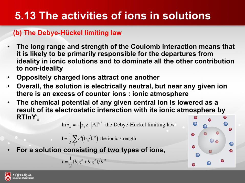
•  The long range and strength of the Coulomb interaction means that it is likely to be primarily responsible for the departures from ideality in ionic solutions and to dominate all the other contribution to non-ideality

•  Oppositely charged ions attract one another •  Overall, the solution is electrically neutral, but near any given ion

there is an excess of counter ions : ionic atmosphere •  The chemical potential of any given central ion is lowered as a

result of its electrostatic interaction with its ionic atmosphere by RTlnϒ±

•  For a solution consisting of two types of ions,

5.13 The activities of ions in solutions (b) The Debye-Hückel limiting law

ln γ± = − z+z− AI1 2 :the Debye-Huckel limiting law

I = 12

z2i bi bΘ( )

i∑ :the ionic strength

I = 12(b+z+

2 + b−z−2 ) bΘ

•  The name ‘limiting law’ was applied because ionic solutions of moderate molalities may have activity coefficients that differe from the values given by Debye-Hückel limitingn law

•  When the ionic strength is high enough,

•  B and C are dimensionless constants and are best regarded as an adjustable empirical parameters

5.13 The activities of ions in solutions (c) The extended Debye-Hückel law

lnγ± = −A z+z− I

1 2

1+BI1 2+CI