linking seasonal and spatial stream carbon dynamics to

Linking Seasonal and Spatial Stream Carbon Dynamics to Landscape Characteristics in Selected Watersheds on the Olympic Peninsula

Roxana Rautu

A thesis Submitted in partial fulfillment of the

Requirements for the degree of

Master of Science

University of Washington 2019

Committee: Bernard Bormann

David Butman Teodora Minkova

Program Authorized to Offer Degree: School of Environmental and Forestry Sciences

i

©Copyright 2019 Roxana Rautu

ii

University of Washington

Abstract

Linking Seasonal and Spatial Stream Carbon Dynamics to Landscape Characteristics in

Selected Watersheds on the Olympic Peninsula

Roxana Rautu

Chair of the Supervisory Committee:

Bernard T. Bormann

School of Environmental and Forestry Sciences

Understanding the factors that affect freshwater export of terrestrially derived carbon is key to creating a

comprehensive model of stream ecology and to developing an accurate carbon budget. Though efforts

have been made to quantify carbon in Pacific Northwest forests, little is known about the carbon in their

freshwater systems. To begin informing this knowledge gap, we collected dissolved organic carbon

(DOC) and water quality data along the stream networks of four small, fish-bearing watersheds in the

Olympic Experimental State Forest on the Olympic Peninsula, WA during the summer and fall of 2018.

Conditional reference random forest models were used to explore how landscape characteristics and

climatic variables affect the spatial and temporal variability of carbon composition and water quality

parameters. We found that slope-related variables and precipitation were the primary drivers of carbon

export. The strengths and magnitudes of these relationships were different for the summer and fall. We

also identified two pools of different carbon composition that were present in three of the four study

watersheds. The results of this study give us a first look at the drivers of carbon export and the quantity

and quality of carbon being exported through freshwater systems. Our work also advises on the spatial

and temporal considerations of stream carbon monitoring. We identify three key questions to pursue in

future studies that will improve our understanding of stream carbon on the Olympic Peninsula and allow

us to monitor it going forward. Our results indicate that future research should explore seasonal

variability, hyporheic influences, and management impacts on carbon dynamics.

iii

Table of Contents

List of Tables ................................................................................................................................................ iv

List of Figures ................................................................................................................................................ v

Chapter 1: Linking Seasonal and Spatial Stream Carbon Dynamics to Landscape Characteristics in

Selected Watersheds on the Olympic Peninsula .......................................................................................... ii

Abstract ..................................................................................................................................................... ii

Introduction................................................................................................................................................ 1

Methods..................................................................................................................................................... 5

Study System and Sample Design........................................................................................................ 5

Field Protocol and Sample Analysis ..................................................................................................... 7

Landscape Metrics Analysis .................................................................................................................. 7

Statistical Analysis ................................................................................................................................ 9

Results .................................................................................................................................................... 10

Watershed Management History and Deciduous Presence ............................................................... 10

Watershed Landscape Analysis .......................................................................................................... 11

Seasonal Carbon Variability ................................................................................................................ 13

Spatiotemporal Patterns of Carbon Variables and Water Quality Parameters ................................... 14

Relationships between DOC, SUVA254, and fDOM ............................................................................. 16

Conditional Random Forest ................................................................................................................ 17

Discussion ............................................................................................................................................... 19

The Olympic Peninsula Mosaic ........................................................................................................... 19

Drivers of Stream Carbon Dynamics .................................................................................................. 20

Identifying Carbon Pools on the Landscape ....................................................................................... 22

Implications for Future Monitoring of Stream Carbon and Water Quality Parameters ....................... 23

Recommendations for Future Studies ................................................................................................ 25

Conclusion............................................................................................................................................... 27

Figures .................................................................................................................................................... 29

Tables ...................................................................................................................................................... 41

References .................................................................................................................................................. 47

Acknowledgements ..................................................................................................................................... 53

iv

List of Tables

Table 1. Summary table of watershed and subwatershed descriptors. The number in parentheses under

“Sample Sites” represents the number of sites sampled in the fall, if different from the summer. ............. 41

Table 2. Median and range values for climatic and landscape variables for all sites. Summer and fall (in

parentheses) values are displayed for climatic variables. VH = Vegetation Height ................................... 42

Table 3. Watershed-scale landscape characteristic values and calculated FRAGSTATS metrics for each

watershed. ................................................................................................................................................... 43

Table 4. Median and range values for stream chemistry throughout summer and fall (parentheses).

Starred variables were not used in data analysis due to data issues or correlation to other variables. ..... 43

Table 5. Mean and standard deviation values (in parentheses) for each carbon and water quality variable

collected at the outlet of each watershed during both seasons. Averages are based on three data points.

Some water quality data is missing in the fall for watershed D due to equipment malfunctioning. ............ 44

Table 6. Measured discharge, DOC concentration, and calculated instantaneous carbon export for the

study watersheds during the three summer (S) and three fall (F) visits. Export values could not be

calculated for the second fall visit for watershed B due to missing discharge data. ................................... 45

Table 7. The R2 value, root mean square error (RMSE), and three most important variables (VI1-VI3) for

each variable from seasonal (summer and fall) conditional reference random forest models. Variable

importance values are reported in parentheses next to the variables. The color of the box represents the

spatial scale of the predictor variable: blue = watershed, green = site, and yellow = climatic. We did not

have enough variability in turbidity during the summer to run a model. ..................................................... 46

v

List of Figures

Figure 1. A map showing the location of the study watersheds, the network sampling design, and the

sample sites. Inset shows the watersheds’ location on the Olympic Peninsula, WA. Lower panels display

the watersheds (black), their corresponding subwatersheds (orange), and the sampling design (red and

yellow stars). Subwatersheds are not labeled in watershed C because we did not sample in them. ........ 29

Figure 2. Maps displaying the watersheds during the summer of 1994 (left) and 2017 NAIP imagery

overlaid with modeled deciduous presence (lime green). White and grey patches in the 1994 photos

represent areas recently harvested, some with exposed bare soil. Polygons overlaid onto the historical

photos represent more recent harvesting activity (mostly thinning) and the year it was completed: yellow

is commercial thinning and red is variable retention harvest. Light green polygons represent older forest.

.................................................................................................................................................................... 30

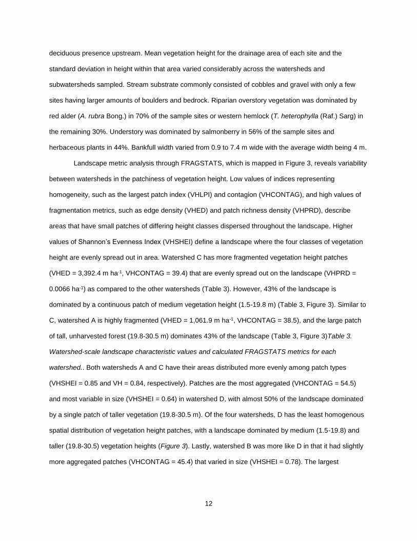
Figure 3. Maps of binned vegetation height classes in each watershed used for landscape metric

analysis. Areas of old forest are delineated in yellow. ................................................................................ 31

Figure 4. Calculated carbon export (g ha-1 hr-1) is plotted with the Hoh River discharge (black line) and

precipitation records in Forks, WA (top solid gray) over the summer and fall field campaigns. Export is

plotted (A) over time and by watershed in the summer (B) and fall (C). ..................................................... 32

Figure 5. Spatiotemporal patterns of conductivity (µS s-1) along the stream networks of the four study

watersheds (A-D). Triangles represent values collected from sub-watershed streams. Yellow boxes

represent summer and blue boxes represent fall. Sample point colors reflect different discharges (m3 hr-1

ha-1) measured at the outlet. ....................................................................................................................... 33

Figure 6. Spatiotemporal patterns of pH along the stream networks of the four study watersheds (A-D).

Triangles represent values collected from sub-watershed streams. Yellow boxes represent summer and

blue boxes represent fall. Sample point colors reflect different discharges (m3 hr-1 ha-1) measured at the

outlet. ........................................................................................................................................................... 33

Figure 7. Spatiotemporal patterns of temperature (ºC) along the stream networks of the four study




Figure 8. Spatiotemporal patterns of % oxygen saturation along the stream networks of the four study




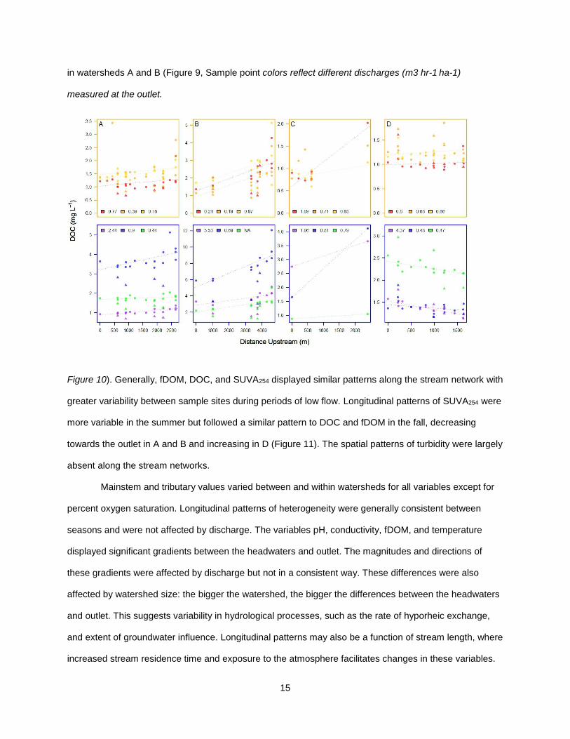
Figure 9. Spatiotemporal patterns of DOC (mg L-1) along the stream networks of the four study




vi

Figure 10. Spatiotemporal patterns of fDOM (RFU) along the stream networks of the four study




Figure 11. Spatiotemporal patterns of SUVA254 (L mg-1 m-1) along the stream networks of the four study




Figure 12. Scatterplots, density plots, and correlation values for DOC (mg L-1), SUVA254 (L mg-1 m-1), and

fDOM (RFU) from all sites. Colors represent the season the data point was collected. ............................ 37

Figure 13. Scatterplots of fDOM (RFU) versus DOC (mg L-1) in each watershed (A-D) and all the

watersheds combined (E). Points are scaled by the corresponding SUVA254 (L mg-1 m-1) value............... 38

Figure 14. DOC (mg L-1) plotted with the most important variables identified by conditional random forest

models. Seasonal linear regressions and the corresponding 95% confidence intervals (shaded areas) are

also plotted with the R2 values reported in the legend. Points are scaled by the corresponding 3-day

precipitation value. ...................................................................................................................................... 39

Figure 15. fDOM (RFU) plotted with the most important variables identified by conditional random forest

models. Seasonal linear regressions and the corresponding 95% confidence intervals (shaded areas) are

also plotted with the R2 values reported in the legend. Points are scaled by the corresponding 1-day

precipitation value. ...................................................................................................................................... 39

Figure 16. SUVA (L mg-1 m-1) plotted with the most important variables identified by conditional random

forest models. Seasonal linear regressions and the corresponding 95% confidence intervals (shaded

areas) are also plotted with the R2 values reported in the legend. Points are scaled by the corresponding

3-day precipitation value. ............................................................................................................................ 40

1

Chapter 1: Linking Seasonal and Spatial Stream Carbon Dynamics to Landscape

Characteristics in Selected Watersheds on the Olympic Peninsula

Introduction

The transfer of material between terrestrial and aquatic systems is a fundamental ecological

process. Climate, hydrological connectivity, and landscape topology all affect the rates and quantities of

terrestrially-derived solutes in a stream at multiple spatial scales (King et al., 2005). A key solute of

interest to researchers and resource managers is carbon. Its export through freshwater streams

represents a significant terrestrial loss of carbon, particularly in Pacific Northwest systems (Butman et al.,

2016; Oliver et al., 2017); however, stream carbon has yet to be fully incorporated into carbon budgets.

Furthermore, the impacts of variability in stream carbon quantity and composition on ecological functions,

the food web, and water quality of Pacific Northwest aquatic systems have been poorly studied. In the

face of climate change and natural and anthropogenic landscape disturbances, questions regarding how

changes in the carbon cycle will affect stream ecology become increasingly important.

Dissolved organic carbon (DOC) is one constituent of stream carbon and a key component of

aquatic life. These solutes serve as important energy sources for aquatic microbes, influence light and

temperature regimes, control pH, and affect the metabolic balance of lakes and streams (Prairie, 2008;

Stanley et al., 2012; Thomas, 1997). They can also affect solubility of toxic metals and organic pollutants

such as mercury (Aiken et al., 2011). The influence of DOC on these stream characteristics is determined

in part by its chemical composition. DOC is composed of non-humic and humic compounds (Wetzel,

2001). Non-humic compounds consist of proteins, simple carbohydrates, amino acids, and lipids that are

usually quickly consumed by heterotrophic bacteria. Humic substances are generally composed of humic

and fulvic acids and humus. These largely hydrophobic aromatics, or chemically stable molecules, are

formed by microbial activity on plant matter; their high molecular weights and complex structures

particularly affect the availability of necessary and toxic metals to aquatic biota (Wetzel, 2001). Dissolved

humic substances have complex effects on cellular processes, microbial growth, and reproductive

outcomes of freshwater organisms that are not well understood (Steinberg et al., 2006). DOC also

contains chromophoric, or colored, dissolved organic matter (cDOM). These brown molecules include

2

tannins that are leached from decaying detritus; in high enough quantities, cDOM can inhibit

photosynthesis by limiting light penetration (Wetzel, 2001). Fluorescent dissolved organic matter (fDOM),

which is the fraction of CDOM that fluoresces, is generally correlated to DOC concentration and can be

measured in situ with specific instruments, providing a mechanism for continual DOC monitoring (Wilson

et al., 2013). Carbon composition is not only important in freshwater ecology but also in treating drinking

water. Chemical disinfectants that are used to purify water can react with humic compounds to form toxic

disinfection by-products such as chloroform (EPA, 2010). Water with a higher concentration of organic

matter not only demands more chlorine to be used in the purification process but also has a higher

potential to form these by-products. The effects of composition and quantity of DOC on water quality

characteristics need to be better understood in natural systems, especially when considering the

treatment of stream water for human consumption.

Both the terrestrial and aquatic carbon cycles influence carbon composition in freshwater. On

land, litterfall, downed woody debris, and root exudation add carbon to the soil (Solinger et al., 2000). The

spatial distribution of ecological and geological weathering functions (Keller, 2019) and decomposition

then determine carbon quantity and composition on the landscape. Soil carbon can be returned to the

atmosphere via respiration, fixated through sorption, or transported to aquatic systems (Keller, 2019).

Generally, allochthonous, or terrestrially derived, carbon is aromatic and composed of particles of high

molecular weight (Mosher et al., 2015). Once in the stream, dissolved carbon can be consumed and

respired by heterotrophic bacteria or carried to the ocean where it is deposited on the coastal shelf,

creating a carbon sink (Abelho, 2001; Butman et al., 2016). DOC can also be produced in situ by

autotrophic aquatic microbes. This autochthonous, or bacterially derived, carbon consists of lower

molecular weight, labile compounds that are often quickly consumed by aquatic heterotrophs (Wetzel,

2001). The processes that drive the allocation of carbon in terrestrial and aquatic systems function at

multiple spatial and temporal scales and are unique to the abiotic characteristics of an area.

Hydrological drivers also determine the composition and amount of carbon delivered to streams.

Barnes et al. (2018) used radiocarbon aging of DOC in U.S. and Arctic waters to develop a framework

illustrating the effects of flow path depth and residence time on carbon dynamics. Shallow flow paths with

low water residence times export higher amounts of aromatic, recently deposited carbon while deep flow

3

paths produce water that is less concentrated in carbon. The DOC present in this subterranean water is

less aromatic and composed of older carbon. Flow path depth also determines the delivery of base

cations and nutrients to the stream, affecting stream metabolism and carbon processing (Battin, 1999). A

gradient of decreasing carbon with increasing soil depth is created as water trickles through the soil

profile and sorption, microbial processing, and remineralization to CH4 and CO2 quickly remove dissolved

carbon compounds (Butman et al., 2016). Thus, the water supplying base flow and groundwater is

typically low in DOC. Dissolved constituents can also undergo transformation in streams by traveling

through hyporheic zones, the areas of sediment below stream beds where groundwater and surface

water mix. These regions can provide a substrate for bacterial biofilms that can either remove or produce

carbon (Schindler & Krabbenhoft, 1998). Hyporheic zones also affect water quality by filtering out

pollutants (Gandy et al., 2007), buffering temperature cycles (Arrigoni et al., 2008), and processing

nutrients (Mulholland et al., 1997). An accurate understanding of a region’s hydrology is crucial for

predicting stream carbon dynamics.

Previous research on stream carbon has primarily focused in natural areas with high amounts of

carbon storage in peat and wetlands. Stream carbon dynamics in these areas have been linked to

landscape attributes such as presence and size of wetlands or peat, mean watershed slope, and forest

soils (Creed et al., 2003; Fellman et al., 2017; Laudon et al., 2011). Studies of headwater streams have

revealed different seasonal patterns of organic and inorganic carbon export (Argerich et al., 2016). The

atmospheric deposition of anthropogenic sulfur and sea salt has also been shown to affect the acidity and

DOC concentration of freshwater systems (Monteith et al., 2007). Though many carbon studies consider

the effects of point sources of carbon, such as wetlands (Walker et al., 2012), few have explicitly related

landscape configuration to carbon fluxes. In order to understand how lateral carbon flux functions in a

watershed, analyses need to be performed at the landscape level.

Studies on the linkage between landscape composition and configuration and resulting stream

chemistry are lacking in the Pacific Northwest. The wet forests of the Olympic Peninsula, WA comprise of

significantly larger accumulations of aboveground biomass as compared to other north temperate forests

and have been extensively managed for timber production (Waring & Franklin, 1979). Though efforts

have been made to quantify carbon in these forests (Gray et al., 2016; Melson et al., 2011), little is known

4

about the carbon in their freshwater systems. Furthermore, the element of human disturbance has not

been assessed, though it is known to affect DOC concentration and composition significantly (Stanley et

al., 2012; Wohl et al., 2017). Data is also scarce on how forest management has affected the aquatic

carbon cycle. Clear-cut areas often export less DOC than unmanaged ones, but the effects of timber

harvests on the direction and magnitude in stream carbon changes are still unclear (Meyer & Tate, 1983;

Stanley et al., 2012). Slashburning can increase soil pH and change the availability of micronutrient

metals and phosphorus in the soil, affecting sorption rates and bacterial communities (Ballard, 2000).

Logging disturbances alter biogeochemical processes in soils by changing soil moisture and temperature

regimes, flow paths, and plant composition (Kreutzweiser et al., 2008). These changes in the soil

chemistry may have had widespread effects on decomposition rates, chemical weathering, and the export

of carbon (Keller, 2019). Timber felling can also induce habitat-specific changes in carbon processing

rates of benthic bacteria in streams (Burrows et al., 2014). Furthermore, landscapes that have received

minimal human development are generally composed of a mosaic of forest seral stages. Current

management practices on the Olympic Peninsula usually involve Douglas-fir plantations, skipping early

seral stages and resulting in homogenous forests dominated by a few species. Eliminating the ecosystem

functions of early and late seral forests could have profound effects on carbon storage and export (Giese

et al., 2003). Exploring the human disturbance dimension will give us new insights into how we can

incorporate carbon fluxes into management decisions.

In this study, we sought not only to expand our knowledge on the spatial and temporal

fluctuations of stream carbon cycling but also to begin informing a key gap in the carbon budget of the

Olympic Peninsula. We asked: how do watershed landscape characteristics influence stream dissolved

organic carbon dynamics? Our objectives were to 1) identify spatial and temporal patterns in carbon

quantity and composition and 2) broadly relate carbon export to landscape composition and configuration.

We expect that some previously established relationships between DOC and landscape characteristics,

such as watershed slope, will be present in our study area. However, due to the variability in

management in the area, we expect to find new relationships between carbon and landscape

composition. This dataset provides a first look at freshwater carbon dynamics for the western Olympic

Peninsula region and identifies potential areas of future research.

5

Methods

Study System and Sample Design

Our study took place in the Clearwater River basin of the Olympic Experimental State Forest

(OESF) on the Olympic Peninsula, WA (Figure 1). The OESF consists of 1,100 km2 of state trust lands

managed by the Washington Department of Natural Resources (WADNR) for revenue production and

ecological values such as long-term productivity and habitat conservation. The specific habitat

conservation strategies, including riparian conservation, are outlined in the habitat conservation plan,

adopted by the state in 1997 (WADNR, 1997). The WADNR’s Forest Land Plan (2016) incorporates

adaptive management to help evaluate its strategy of creating a shifting mosaic of seral stages on its

lands (WADNR, 2016). The goal is to manage the landscape to create a balance of early/mid/late seral

conditions to maintain biodiversity, including the survival of specific late-seral species such as Spotted

Owls and Murrelets. A distinct conservation goal is to provide habitat for viable salmonid populations. This

conservation plan is distinct from the management strategies of the U.S. Forest Service and other DNR

lands that take the approach of permanent fixed reserves.

The region experiences a mild maritime climate and heavy precipitation, ranging from 203 cm to

355 cm per year. Most of this precipitation falls as rain between October and March (Halofsky et al.,

2011). The steep terrain and well drained soils create flashy stream responses with rapid times-to-peak

during rain events (Minkova & Devine, 2016). Thus, we expect the first fall rains to mobilize the carbon

pool that was built up over the summer and produce the most DOC per unit of discharge (Wilson et al.,

2013). Western hemlock (Tsuga heterophylla (Raf.) Sarg.), Sitka spruce (Picea sitchensis (Bong.)

Carriére), and Douglas-fir (Pseudotsuga menziesii (Mirb.) Franco) dominate the landscape with red alder

(Alnus rubra Bong.) common in riparian and recently disturbed areas (Franklin & Dyrness, 1988).

Understory vegetation primarily consists of salal (Gaultheria shallon Pursh), salmonberry (Rubus

spectabilis Pursh), and sword fern (Polystichum munitum (Kaulf.) C. Presl). The Clearwater River is a

mixed bedrock and alluvial stream (Wegmann & Pazzaglia, 2002). Underlying lithology primarily consists

of greywacke in the center of the Peninsula and glacial till closer to the coast.

The four watersheds chosen for this study were designated as part of the Large-Scale Integrated

Management Experiment, referred to as the Type 3 (T3) Watershed Experiment (Bormann & Minkova,

6

2017). A Type 3 stream is the smallest fish-bearing stream size. This collaborative effort between the

WADNR and the University of Washington (UW) looks to evaluate ecosystem sustainability with both

environment and community wellbeing goals by comparing the OESF Forest Land Plan, a 100-year

landscape management plan (WADNR, 2016), to two other management strategies and a no-action

control. Samples were collected in the four watersheds receiving the “Accelerated” treatment that will test

innovative management strategies, including riparian harvesting, across watersheds. We chose to focus

on this treatment because the intensity of the treatments will best allow us to relate management effects

to changes in stream carbon. Within each of the four “Accelerated” watersheds, sub-watersheds, which

are catchments of the tributaries to the mainstem, were delineated by WADNR scientists based on

drainage size. Harvesting treatments will be implemented in a randomly chosen sub-watershed in each

“Accelerated” watershed. Currently, all watersheds are at least 95% forested. Watershed and sub-

watershed characteristics and general management history are summarized in Table 1.

Sampling design was determined with three main objectives in mind. We wanted to 1) explore the

spatial scales at which DOC variation could be compared to watershed characteristics, 2) determine the

spatial and temporal scales at which future monitoring could capture DOC dynamics, and 3) provide pre-

treatment carbon data for the T3 Experiment. To achieve these goals, we devised a longitudinal sampling

design along the stream networks. We collected samples at the T3 outlet, at sub-watershed confluences,

and at points along the mainstem to create a sampling density of a sample every 0.2 miles or less. We

collected three samples at each sub-watershed confluence: one in the sub-watershed tributary, one in the

mainstem before the confluence, and one after the sub-watershed tributary and mainstem had fully mixed

(Figure 1). It was assumed that DOC concentration would change minimally over less than 0.3 km, so the

sample after the mixing of sub-watershed Ba04 and the mainstem was omitted due to its proximity to

Ba03. The sampling method had to be altered in watersheds B and C due to time constraints and difficult

terrain respectively. To explore the effects of different hydrological conditions, we conducted six field

campaigns per watershed in 2018: three in the summer (7/16 – 8/15) and three in the fall (10/10 – 11/1).

Some sites in watersheds A and C could not be visited in the fall due to high flow conditions (Figure 1).

We collected 187 summer and 168 fall samples in total.

7

Field Protocol and Sample Analysis

For DOC sampling, we used a 60mL Luer-Lok Syringe with a 0.7 µm Whatman GF/F glass

microfiber filter to filter 120 ml (two full syringes) of stream water into acid-washed Nalgene bottles. Water

temperature, pH, conductivity, total dissolved solids (TDS), turbidity, fluorescent dissolved organic matter

(fDOM), and % oxygen saturation were recorded using a YSI Exo 2 Sonde during each site visit in order

to characterize stream chemistry in each watershed. Furthermore, we wanted to quantify the relationship

between fDOM and DOC concentration to allow for DOC monitoring in the future. To ensure accuracy,

Sonde measurements were taken every 15-20 seconds for 3-5 minutes and then averaged during data

processing. We were unable to measure chlorophyll values but expect it was low given the known

oligotrophic nature of these streams (Fevold, 1998). Samples and filters were kept cool in the field and

then frozen upon returning to the lab. Discharge was measured at the outlet with a Marsh-McBirney when

the outlet sample was collected. The same cross-section of the river was measured during the summer

and fall field campaigns. Site characteristics such as overstory and understory species composition and

streambed substrate composition were estimated as percentage of cover.

Samples were allowed to reach room temperature before being run on the UW Shimadzu Total

Organic Carbon (TOC-L) Analyzer within a week of collection. We calculated carbon export for these

watersheds using the discharge measured at the outlet and DOC concentration. Samples were also

analyzed on the UW Horiba Aqualog® to obtain fluorescence and absorption data. We used the

absorbance values at 254 nm and DOC concentration to calculate specific ultraviolet absorbance at 254

nm (SUVA254). This value is correlated to the proportion of aromatic content in a DOC sample (Weishaar

et al., 2003). Aromatic, or humic, carbon molecules are produced by microbes breaking down organic

matter (Wetzel, 2001). Thus, high SUVA254 values are indicative of allochthonous, or litter-derived, carbon

sources versus autochthonous, or aquatic bacteria-derived, carbon pools.

Landscape Metrics Analysis

Analyses were performed in ArcGIS v10.4 for the drainage area of each sample site. Pre-

processed spatial data was prepared by the T3 Experiment Analysis team and downloaded from the

WADNR GIS Portal (http://data-wadnr.opendata.arcgis.com/). We used a high spatial resolution (1 x 1 m),

LiDAR-derived digital elevation model (DEM) and shapefiles of the watersheds to calculate multiple

http://data-wadnr.opendata.arcgis.com/

8

landscape characteristics (Table 2). We additionally chose to calculate flow-weighted slope (FWS), which

combines flow accumulation and slope values of a watershed area, because it is a metric that has been

linked to stream chemistry and is not affected by watershed size (Walker et al., 2012). FWS for a

watershed is correlated to mean slope, but its calculation weights the slopes near a stream more heavily

than those further away. Using the WADNR’s RS-Hydro, a LiDAR-based model for mapping stream

types, we estimated the mean stream slope (MeanStreamSlope) and mean stream elevation

(MeanStreamElevation) for the modelled types 3, 4, and 5 streams upstream of each site. We used a

shapefile of modeled unstable slopes of DNR managed surface and timberlands to calculate the percent

of a watershed’s area that was modeled as unstable (ModeledUnstable). This model, which incorporates

slope-statistics and lithology, is used by the WADNR as a conservative estimate to identify areas that

need further geological assessment before allowing harvesting. Like watershed slope, we expect that

slope stability is indicative of soil erosion rates and water residence time, both of which affect the

distribution and transport of terrestrial carbon (Barnes et al., 2018; Lal, 2003).

Aboveground biomass is a key source of carbon for streams in the Pacific Northwest (Fellman et

al., 2017; Lajtha & Jones, 2018). Previous studies have established correlations between LiDAR-derived

vegetation, or canopy, height (VH) and biomass characteristics such as stand height, volume, and basal

area (Dubayah & Drake, 2000; Knapp et al., 2018). These characteristics are also related to stand age

and the resulting attributes and functions of those forests (Means et al., 2000). Using canopy height as a

proxy for forest function, we wanted to see how variability in VH as well as its distribution on the

landscape could affect stream carbon and water quality parameters. To get at the variability, we

calculated the mean, standard deviation, and maximum VH for the drainage area of each sample site. For

those areas, we also explored vegetation distribution across the landscape by calculating 5 landscape-

level metrics in FRAGSTATS v4.2.1.603 using the 8-neighbor rule (McGarigal & Marks, 1995). The 8-

neighbor rule considers two pixels of the same value to be in the same patch if they are horizontally,

vertically, or diagonally adjacent. To minimize computing time, the VH raster was aggregated from 1 x 1

m pixels to 10 x 10 m pixels and reclassified into height bins of 0-5, 5-65, 65-100, and 100+ feet to create

patches of these bins on the landscape. The metrics we chose are described in Table 2 and were picked

to explore how evenly the patches were distributed on the landscape and how patch composition varied.

9

Litter from deciduous trees and shrubs also contribute to stream carbon export through direct

input of organic material and annual renewal of the soil carbon pool (Mcdowell & Fisher, 1976).

Evergreen conifers and shrubs in this area tend to produce litter that is lower in decomposability and

quantity (Prescott et al., 2000). For these reasons, we expected that variability in the presence of

deciduous vegetation in these watersheds could affect DOC concentrations. We used 1 ft. commercial-

grade 4 band cable inspection robot (CIR) LiDAR data to train samples in an area with known deciduous

presence north of our study site. We then applied the classification signatures to 1 m resolution, 4 band

CIR obtained from the USGS for each of our study watersheds. We applied Block Statistics using 4 x 4m

blocks and the Sum function to yield values from 0 to 16 for each block. Zero indicates no deciduous cells

and 16 indicates that all cells were deciduous. We then resampled the Block Statistics raster using the

Majority function to convert the blocks to 4m square cells with the 0 to 16 values retained. Through visual

inspection of obvious deciduous stands along roads, for example, we determined that 100% likelihood of

deciduous presence (the value of 16) produced acceptable results.

Changes in temperature and precipitation have been linked to stream DOC responses by

affecting microbe metabolism (Gillooly et al., 2001) and mobilization of carbon (Bianchi et al., 2013),

respectively. Daily climatic data for Forks, WA, the nearest data source to our study area, was obtained

from the U.S. Climate website (“U.S. Climate Data,” 2019). From this data, we created three variables: the

amount of precipitation that fell on the day the data was collected (1DayPrecip), the total precipitation that

had fallen during the day of collection and two days prior (3DayPrecip), and the cumulative degree days

over the day of data collection and two days prior (3DayDD50). Degree day was calculated by subtracting

50 ºF from the daily average, which is the daily high minus the daily low divided by two.

Statistical Analysis

Classification and regression trees (CARTs), or decision trees, are a useful way to model

complex relationships between predictor and response variables in part because they don’t assume

normal distributions, can account for spatial autocorrelation in the data, and handle complex interactions

between variables (Breiman et al., 1984). They are formed through binary recursive partitioning of the

data and offer a simple interpretation of the effects of different predictor variables on a response variable.

Olden et al. (2008) describe the benefits and drawbacks of CART analysis in greater detail. However, a

10

single decision tree is highly prone to overfitting and error. This can be accommodated by using bootstrap

sampling of the data to generate hundreds of CARTs and create a ‘random forest’. The ‘random’ aspect

refers to the algorithm’s strategy to try a subset of the predictor variables at each node. This method

averages across all bootstrap estimates and calculates variable importance, which is evaluated by

reduction in model error. Furthermore, we chose to use a specific kind of decision tree algorithm called

conditional inference trees. Unlike other decision trees, conditional trees provide a unified framework that

handles selection bias towards variables with more possible splits and overfitting of the data (Sardá-

Espinosa et al., 2017).

We grew a separate conditional random forest model for each season (summer and fall) for

dissolved organic carbon (DOC), specific ultraviolet absorbance at 254 nm (SUVA254), fluorescent

dissolved organic matter (fDOM), pH, conductivity, turbidity, percent oxygen saturation, and temperature

using the data from all sites. Decision trees are not affected by spatial autocorrelation, allowing us to use

all the data collected (Hijmans & Ghosh, 2019). The predictor variables we used in our conditional forest

models are listed in Table 2. Discharge was not used as a predictor variable due to missing data. We did

not run models for total dissolved solids or turbidity because of correlation to conductivity and low

variability in values, respectively. Models were developed using the ‘caret’ and ‘party’ packages in R

version 3.5.1 (R Core Team, 2018). First, we optimized the number of predictor variables to try at each

node using conditional forests and Out-Of-Bag (OOB) error. Then, using the number of predictors that

produced the lowest error, we grew 1000 conditional inference trees for each response variable. Variable

importance was computed by permuting the predictor variable values and assessing the consequent

effect on model error (Breiman, 2001). The larger the increase in model error, the more important that

variable predictor was deemed.

Results

Watershed Management History and Deciduous Presence

Through visual inspection of historical photos from Google Earth (1984-Present) and the available

WADNR’s harvesting records (1992-Present), we broadly summarized management history in each

watershed (Table 1). All watersheds experienced extensive clear-cutting during the 1980s and early

1990s with lax regulations on soil disturbance and an absence of riparian buffers. The large amounts of

11

logging slash associated with harvesting older forests were broadcast burned to open up planting spots

where mostly Douglas-fir was planted within two years of cutting, as per WADNR standards. Red alders

were likely present initially but were mostly removed with herbicides. They remain in riparian areas, along

the roads, and other areas of disturbed soil. WADNR records indicate that intensive harvesting activity

ceased in watersheds C and D approximately 30 years ago (Figure 2). Watersheds A and B have

experienced small areas of more recent clear-cut like harvests (called variable retention harvests) and

more extensive commercial thinning, though the extents and intensities of these disturbances are

significantly lower than those of the 1980s and earlier. Older, unmanaged forest was present in all

watersheds with watershed C having the largest patch. Though our historical analysis only went back to

the 1980s, the spatial distribution of the old forest patches suggests these watersheds experienced

intensive harvesting down to the stream edges in the 1960s and 1970s.

We wanted to explore whether the variability in the size of the carbon pool generated by

deciduous vegetation affected stream chemistry. When visually comparing modeled deciduous presence

to landscape composition in 1994, we see more deciduous presence (lime green) in recently disturbed

areas (white and gray areas) and along roads (Figure 2). In addition, deciduous vegetation appears to be

more common on south and east facing slopes. The amount of deciduous presence varied between the

watersheds. Surprisingly, we find the highest percentage of the landscape as deciduous in watershed D

and the lowest amount in watershed A, suggesting a negative relationship between deciduous presence

and continued management (Table 3). These patterns may be due to reduced use of herbicides to control

for alder in more recent harvests, exposure of understory vegetation through gaps in the canopies of

conifer stands, and natural disturbances such as stream floods. The management practices and timing of

the harvesting before the 1990s may have also affected the patterns of deciduous flora on the landscape.

Our model provides only a conservative estimate of deciduous presence. Improving model accuracy by

correcting for the spectral signature of young conifers and ground-truthing is needed to better understand

the relationship between deciduous presence and management.

Watershed Landscape Analysis

Landscape characteristics for all sample sites are described and summarized in Table 2. Most of

the draining watersheds spanned lower elevations, had medium to steep slopes and contained little

12

deciduous presence upstream. Mean vegetation height for the drainage area of each site and the

standard deviation in height within that area varied considerably across the watersheds and

subwatersheds sampled. Stream substrate commonly consisted of cobbles and gravel with only a few

sites having larger amounts of boulders and bedrock. Riparian overstory vegetation was dominated by

red alder (A. rubra Bong.) in 70% of the sample sites or western hemlock (T. heterophylla (Raf.) Sarg) in

the remaining 30%. Understory was dominated by salmonberry in 56% of the sample sites and

herbaceous plants in 44%. Bankfull width varied from 0.9 to 7.4 m wide with the average width being 4 m.

Landscape metric analysis through FRAGSTATS, which is mapped in Figure 3, reveals variability

between watersheds in the patchiness of vegetation height. Low values of indices representing

homogeneity, such as the largest patch index (VHLPI) and contagion (VHCONTAG), and high values of

fragmentation metrics, such as edge density (VHED) and patch richness density (VHPRD), describe

areas that have small patches of differing height classes dispersed throughout the landscape. Higher

values of Shannon’s Evenness Index (VHSHEI) define a landscape where the four classes of vegetation

height are evenly spread out in area. Watershed C has more fragmented vegetation height patches

(VHED = 3,392.4 m ha-1, VHCONTAG = 39.4) that are evenly spread out on the landscape (VHPRD =

0.0066 ha-1) as compared to the other watersheds (Table 3). However, 43% of the landscape is

dominated by a continuous patch of medium vegetation height (1.5-19.8 m) (Table 3, Figure 3). Similar to

C, watershed A is highly fragmented (VHED = 1,061.9 m ha-1, VHCONTAG = 38.5), and the large patch

of tall, unharvested forest (19.8-30.5 m) dominates 43% of the landscape (Table 3, Figure 3)Table 3.

Watershed-scale landscape characteristic values and calculated FRAGSTATS metrics for each

watershed.. Both watersheds A and C have their areas distributed more evenly among patch types

(VHSHEI = 0.85 and VH = 0.84, respectively). Patches are the most aggregated (VHCONTAG = 54.5)

and most variable in size (VHSHEI = 0.64) in watershed D, with almost 50% of the landscape dominated

by a single patch of taller vegetation (19.8-30.5 m). Of the four watersheds, D has the least homogenous

spatial distribution of vegetation height patches, with a landscape dominated by medium (1.5-19.8) and

taller (19.8-30.5) vegetation heights (Figure 3). Lastly, watershed B was more like D in that it had slightly

more aggregated patches (VHCONTAG = 45.4) that varied in size (VHSHEI = 0.78). The largest

13

continuous patch only took up 27% of the watershed area, but much of the landscape is dominated by

medium and taller vegetation heights like watershed D (Figure 3).

The results of this analysis indicate that harvesting practices created large patches of younger,

shorter forests. Though we see some variability between the watersheds, the metrics do not indicate that

watersheds A and B, which are have been managed more recently, differ significantly from the other two

watersheds. This variability may be attributed to differences in management planning in these areas and

watershed size (larger areas are generally more heterogeneous). Furthermore, areas of older forest

(yellow outlines) differed in configuration and composition from managed areas, with taller vegetation and

smaller, heterogeneously distributed patches (Figure 3). This variability may be indicative of smaller scale

disturbances such as wind or disease.

To characterize the physical properties of each watershed, we also report the mean values of

calculated watershed-scale landscape characteristics and calculated metrics for each watershed in Table

3. We see the biggest differences between watersheds when looking at slope variables and deciduous

presence. Watershed C is significantly steeper than the others while B generally has the lowest slopes.

Watershed D is modeled to have at least twice as much deciduous cover as compared to the rest of the

watersheds. Though watersheds A and D have similar mean slopes, the higher FWS in D suggests that

riparian slopes are steeper. Both underlying lithology and mean slope contributed to modeled slope

stability. Watersheds with higher amounts of glacial till, such as watersheds A and D, were estimated to

have more unstable slopes than watersheds that were primarily greywacke, like B and C. The

heterogeneity in sediment size of glacial till increases slope instability more than the compact rock sheets

of greywacke do. Thus, even though watershed C is significantly steeper than A and D, the underlying

greywacke creates better slope stability.

Seasonal Carbon Variability

Our sampling campaigns captured primarily warm and dry conditions in the summer and a few fall

precipitation events (Table 2). Ranges of the carbon variables (DOC, SUVA254, and fDOM) and water

quality parameter values for each season from all sites are summarized in Table 4. Temperature declined

in the fall as expected. SUVA254 remained largely unchanged between seasons. Other variables

increased in the fall relative to the summer. Fall values also had increased variability for all characteristics

14

except for pH and decreased temperature variability. Stream parameters are summarized by watershed in

Table 5. Watershed B is characterized as warm, slightly acidic, having lower conductivity, and producing

the highest carbon concentrations. On the other end of the spectrum, C is colder, slightly basic, having

higher conductivity, and producing low carbon concentrations. Despite its proximity to B, watershed A is

more similar in pH and temperature to C but has higher concentrations of carbon than C does. D is more

like B with regards to pH, temperature, and SUVA254 values but generally has lower carbon

concentrations than B does.

Instantaneous carbon export, which was calculated for every stream visit, generally increased

during the fall in all watersheds (Table 6). Peak export coincided with the highest flows, not the highest

DOC concentrations. DOC concentrations did not display a clear relationship with discharge, suggesting

that changing conditions and spatial heterogeneity of terrestrial carbon pools exist. Watershed carbon

export decreased during dry periods and increased quickly with precipitation events (Figure 4). Rain

events in September may have contributed to the high carbon export values during the beginning of our

fall sampling despite the lower discharge. Carbon export continually increased in the summer for

watersheds B and C while remaining relatively constant for A and D. In the fall, the same rain event

triggered a larger increase in carbon export in watershed D versus watershed A, possibly due to regional

variability in precipitation.

Spatiotemporal Patterns of Carbon Variables and Water Quality Parameters

The spatial patterns of carbon variables and water quality parameters varied along the

longitudinal position in the stream networks of our four study watersheds (Figures 5 to 11). Temperature

generally increased as water moved towards the outlet, except for during two fall field visits in watershed

A and one in D (Figure 7). Baseflow, which supplies the headwaters, is generally cooler than surface flow,

which increasingly contributes to a river further downstream. Modifications of this longitudinal pattern

suggests a change in hydrological sources and connectivity. Oxygen saturation was generally over 80%

throughout all watershed networks and displayed an increasing trend towards the outlet (Figure 8). In A

and B, conductivity and pH increased and fDOM and DOC decreased in a downstream direction while the

opposite pattern occurred in watershed D. This downstream increase in DOC and fDOM in D can partly

be attributed to its tributaries acting as higher sources of these carbon components relative to tributaries

15

in watersheds A and B (Figure 9, Sample point colors reflect different discharges (m3 hr-1 ha-1)

measured at the outlet.

Figure 10). Generally, fDOM, DOC, and SUVA254 displayed similar patterns along the stream network with

greater variability between sample sites during periods of low flow. Longitudinal patterns of SUVA254 were

more variable in the summer but followed a similar pattern to DOC and fDOM in the fall, decreasing

towards the outlet in A and B and increasing in D (Figure 11). The spatial patterns of turbidity were largely

absent along the stream networks.

Mainstem and tributary values varied between and within watersheds for all variables except for

percent oxygen saturation. Longitudinal patterns of heterogeneity were generally consistent between

seasons and were not affected by discharge. The variables pH, conductivity, fDOM, and temperature

displayed significant gradients between the headwaters and outlet. The magnitudes and directions of

these gradients were affected by discharge but not in a consistent way. These differences were also

affected by watershed size: the bigger the watershed, the bigger the differences between the headwaters

and outlet. This suggests variability in hydrological processes, such as the rate of hyporheic exchange,

and extent of groundwater influence. Longitudinal patterns may also be a function of stream length, where

increased stream residence time and exposure to the atmosphere facilitates changes in these variables.

16

The effects of discharge on carbon quantity and water quality parameter values varied by season

and watershed. Though two of the field campaigns in D in the fall had similar discharge, they show

significantly different conductivity, pH, temperature, DOC, and fDOM values while SUVA254 and percent

oxygen saturation did not change (Figures 5 to 11). A similar effect is seen in watershed C in the fall, but

our interpretation is limited due to only having two data points per field campaign. In A and B, we

captured bigger differences in discharge during both seasons, but there were no consistent stream

responses to changes in flow. Conductivity generally displayed a positive relationship with discharge in

the summer and a negative one in the fall. Higher discharge resulted in lower DOC but surprisingly higher

SUVA254 and fDOM values. The highest concentrations of DOC were recorded in the fall during medium

flow (Figure 9). The highest values of SUVA254 and fDOM occurred during the highest flows in the fall

(Figure 10, Figure 11).

Relationships between DOC, SUVA254, and fDOM

Our sampling period was generally characterized by low DOC concentrations and high SUVA254

and fDOM values. We did not capture significant variability in discharge or precipitation; however, our

data shows variability in the relationships between fDOM, SUVA254, and DOC (Figure 12). This variability

provides key information for understanding the sources of stream carbon. The highest and lowest values

of SUVA254 occurred during the fall and values generally displayed a positive relationship with discharge.

Dissolved organic carbon and fDOM values peaked in the fall and had the lowest values in the summer,

though the range of fall values encompassed those of the summer. The relationship between DOC and

SUVA254 is weakly negative (ρ = -0.32) in the fall and weakly positive (ρ = 0.31) during the summer. The

highest values of SUVA254 occurred at relatively low values of DOC while samples of high DOC had very

low SUVA254, but there is no clear linear relationship between the two variables (Figure 12). Variability in

this relationship could suggest that there are multiple carbon pools of different aromaticity contributing to

the stream. Furthermore, we expect SUVA254 and fDOM to be correlated as they are often indicative of

similar allochthonous carbon pools generated by decaying vegetation. We see a weak positive correlation

between SUVA254 and fDOM in the fall (ρ = 0.4) and a slightly stronger one in the summer (ρ = 0.65).

Again, there is no clear linear relationship between SUVA254 and fDOM, but the relationship across the

seasons is weakly positive (ρ = 0.48; Figure 12). We found a strong overall correlation between fDOM

17

and DOC (ρ = 0.68), but there are two distinct positive relationships that appear during both seasons.

These two relationships are present in at least watersheds A, B, and D (Figure 13). We note that the

steeper slope between fDOM and DOC is characterized by higher SUVA254 values while the gentler slope

has low values. The distinct relationships we observed between the carbon variables suggest that the

carbon in the stream is originating from at least two different carbon pools: one that is richer in aromatic

carbons (estimated by SUVA254) and tannins (fDOM) and another that has as higher proportion of labile

carbon. We cannot confirm whether both carbon pools are present in watershed C as it did not display

much variability in any of the carbon variables; this may be due to limited sampling and lack of variability

in discharge conditions.

Conditional Random Forest

We report the R2 and RMSE of the seasonal conditional forest models and the top three

predictors with their importance values for each response variable modeled (Table 7). Model performance

(R2) varied between seasons and between variables. Generally, watershed-scale variables, especially

those related to slope, and climatic variables were the most important in the models. Fall models were

less accurate (higher RMSE) than summer models for all variables except temperature and percent

oxygen saturation. Site-level characteristics were important for the summer models of fDOM, pH and

conductivity and both seasonal models of percent oxygen saturation. The top three response variables

most accurately modeled by our predictor variables (highest R2 values) were fDOM, pH, and conductivity.

The turbidity, % oxygen saturation, and DOC seasonal models were the least accurate (lowest R2

values). Models that reported “Watershed”, which refers to the study watershed name, as an important

predictor suggest that our study watersheds have significantly different values for the corresponding

variable.

The seasonal models for carbon variables (DOC, SUVA254, and fDOM) vary in accuracy and

important predictor variables (Table 7). Mean slope and percent of watersheds that are modeled as

unstable slopes are strong predictors during both seasons for DOC, suggesting that underlying lithology

influences carbon concentration. Precipitation was an important variable in predicting fall DOC. Only

climatic variables were important for predicting SUVA254 in the fall. The summer SUVA254 model uses the

watershed-scale slope predictors and watershed name as the top predictors. Conditional random forest

18

most accurately models both summer (R2 = 0.83) and fall (R2 = 0.85) fDOM data. Mean slope is an

important variable in both seasons. The summer model also uses the percent of Douglas-fir at the site

and percent of the draining landscape that is modeled as deciduous. In the fall model, 1-day precipitation

and mean stream slope replace those two predictors. We note that the importance values for the second

and third most important variables in both seasonal models are significantly lower than the values for the

most important variable, mean slope.

Landscape and climatic variables do well at predicting pH, conductivity, and temperature but not

turbidity or oxygen saturation. The fall and summer pH models performed similarly well. Mean slope and

watershed were important variables with elevation and 1-day precipitation being important in the summer

and fall respectively. The conductivity summer model had the same predictors as the pH summer model

but placed a greater importance on the watershed name. Fall conductivity was driven by watershed name

and precipitation. The stream temperature seasonal models were primarily driven by air temperature

variables. Fall temperatures (RMSE = 0.31) were more accurately predicted than summer temperatures

(RMSE = 0.50). The poor precision of the turbidity and percent oxygen models can be attributed to either

lack of variability in the data collected as compared to the variability in landscape and climatic

characteristics or the absence of a relationship between the predictor and response variables.

We found seasonal negative relationships between DOC and mean slope (Figure 14). Lower

slope areas showed more variability in DOC export during the fall than did high slope areas. This resulted

in a steeper slope in the fall for the seasonal fitted linear regressions. fDOM displayed similar seasonal

negative relationships with mean slope (Figure 15). SUVA254 had a negative relationship with mean slope,

but unlike fDOM and DOC, it did not differ between seasons (Figure 16). Furthermore, mean slope did not

affect the variability of SUVA254 values as it did for fDOM and DOC. Precipitation had a significant effect

on all three variables. Increased precipitation resulted in higher fDOM and SUVA254 but lower DOC. The

significant effect of this climatic variable in the fall resulted in poor accuracy of the SUVA254 fall linear

regression model (R2 = 0.01).

19

Discussion

The Olympic Peninsula Mosaic

We found that the study watersheds experienced a drastic decrease in management intensity

during the 1990s. Throughout the 1970-80s, harvesting operations created large clear-cuts on the

landscape with lax regulation of ground disturbance and performed high intensity slash burns, leaving

only small areas of untouched forest. Since the 1990s, the WADNR has transitioned to primarily lower

impact pre-commercial and commercial thinning, variable riparian buffers, and small areas of variable-

retention harvest with some pile burning. Landscape metric analyses revealed how previous management

homogenized the distribution of vegetation heights in our study watersheds. This is best observed when

comparing the configuration and patch sizes between untouched forest and managed areas (Figure 3).

Inspection of the large patch of untouched, older forest in watershed C suggests that these natural forests

consist of smaller, heterogeneously distributed patches of tree ages. However, we did not see a signal in

the stream chemistry from these untouched forests, suggesting that the FRAGSTATS analysis we used

may not capture important differences in forest configuration and composition. Furthermore, the areas of

untouched forest were small, dispersed on the landscape, and interspersed with managed areas, which

may have diluted any “old forest” signals. Though we used vegetation height as a proxy for biomass, it did

not account for forest floor biomass, which we expect to be higher in untouched forests. Thus, the

vegetation height bins and configuration metrics we used most likely did not capture variability in forest

function or carbon pool size. However, we expect that creating large, homogenous patches of younger

forests on the landscape has implications for stream carbon by reducing soil carbon storage (Sun et al.,

2004), altering hydrology (Moore & Wondzell, 2005), and impacting biodiversity (Halpern & Spies, 1995).

Though our watersheds displayed some variability in the configuration and intensity of managed

areas, we cannot directly relate management activities to stream chemistry because these differences are

confounded by variability in watershed landscape characteristics, which were identified as primary drivers

of multiple stream variables. Landscape characteristics partly determine the intensity and management

techniques that the WADNR can apply to an area. For example, the stability and steepness of slopes will

affect the accessibility of the timber as well as the harvesting techniques used by loggers. This could

create a correlation between accessibility, which is primarily driven by slope, past harvesting, and

20

distance to roads, making it difficult to isolate the effects of either variable on stream carbon dynamics.

We also expect that the intensive and widespread management of the 1970-80s left stronger legacy

effects on the landscape than more recent management, which is smaller in scale. However, the

prevalence of this management history in our watersheds makes it difficult to identify the consequences

of these changes to stream chemistry. Lastly, we must also consider that the effects of logging on stream

carbon export were most prevalent right after the harvesting and that the system may have recovered to a

point where the induced changes are minimal or nonexistent.

Drivers of Stream Carbon Dynamics

Our results suggest that lithology, climatic conditions, and physical properties of watersheds drive

carbon dynamics on the Olympic Peninsula. These variables are inter-dependent at multiple spatial and

temporal scales and affect both the quality and quantity of carbon that is exported by the land. We found

the strongest predictors of carbon variables to be slope related. Both DOC and fDOM had a steeper

negative relationship with mean slope during the fall as compared to the summer (Figure 14, Figure 15).

Areas with gentler slopes have slower percolation rates, allowing the water to leach more carbon from the

soil before reaching the streams. The relationship between SUVA254 and mean slope did not vary by

season. Aromatic carbon is hydrophobic, so we would not expect increased water residence time to affect

solubility rates. Unlike the study conducted by Walker et al. (2012) in the headwater streams of the Kenai

Lowlands, Alaska, we did not find flow-weighted slope (FWS) to be an important predictor, meaning

stream carbon is not as affected by riparian slope steepness in these watersheds. This suggests that

hydrological connectivity extends past riparian areas, connecting upland sources of carbon and

overwhelming the effects of differences in riparian slopes.

We also did not find a relationship between the size of the drainage area and carbon dynamics at

a sampling site. Area drained is positively correlated with stream length and the amount of time a carbon

compound has spent in the aquatic system. The lack of a relationship between area drained and carbon

dynamics suggests that the streams vary in hydrological characteristics. This is reflected in the different

longitudinal patterns of DOC concentrations we observed in our study watersheds. In watersheds A and

B, increasing the area drained, or moving towards the outlet, results in a lower DOC concentration while

the opposite pattern is observed in D (Figure 9). In addition to the influences of the tributaries in these

21

watersheds, a decrease in DOC along the stream network could suggest carbon processing especially in

the hyporheic zone or dilution through the groundwater inputs (Corson-Rikert et al., 2016). These

influences may be driven in part by lithology, where the porosity of the underlying stream bed affects

hyporheic zone properties. Furthermore, landscape structure, topology, and catchment wetness affect the

spatial pattern of upland-stream connectivity (Jencso et al., 2009). Variability in these components

between our watersheds will have also determined hydrological connectivity, and consequently the

longitudinal patterns of carbon concentrations.

Climatic variables were important in multiple carbon and water quality parameter models,

particularly in the fall when we captured variability in precipitation and discharge. Seasonal changes in

soil moisture and hydrological connectivity most likely resulted in the temporally inconsistent

DOC/discharge relationship we observed (Wilson et al., 2013). We also found that SUVA254 was strongly

driven by precipitation and air temperature and resulted in a changing relationship with DOC. This is most

likely due to precipitation inputs enabling the leaching of surface humic material into the stream via

overland, or surficial, flow (Inamdar et al., 2011). The positive relationship between SUVA254 and

discharge we found is similar to the one observed by Hood et al. (2006) in the H.J. Andrews Experimental

Forest, Oregon. This suggests that a similar hydrologic mechanism is at work in our watersheds where

more aromatic carbon is mobilized during high flow events through increased hydrological connectivity to

near-surface soils. The researchers also found higher SUVA254 values exported by previously harvested

catchments. Though we found significantly higher SUVA254 values than Hood et al. (2006), we were

unable to identify a relationship between SUVA254 values and harvesting history. Some areas that drained

primarily old forest also had recent clear-cuts in them, making it impossible to differentiate between the

SUVA254 contributions of old and young forests. Dissolved iron, which we did not measure, has also been

shown to affect absorbance and may have contributed to the high SUVA254 values (Weishaar et al.,

2003). Small patches of orange iron deposits were observed in some of the streams. In order to relate

carbon composition and quantity to management history explicitly, we need more data collected across

seasons in watersheds that have higher variability in management history as well as watersheds with no

previous management. Data collected under different climatic conditions will also help us better

22

understand how the interaction between precipitation and landscape characteristics affect terrestrial

carbon export to the streams.

Identifying Carbon Pools on the Landscape

Our data suggests that there are two pools of different carbon composition on the landscape that

are present in at least three of the four study watersheds (Figure 13). One has a higher proportion of

aromatic content (SUVA254) and fDOM but low overall DOC; the other has very low SUVA254 and lower

fDOM but higher concentration of overall DOC. The contribution of the highly aromatic pool to the stream

is correlated with the amount of precipitation received 3 days before data collection (Figure 16). The

chemical makeup of this carbon source and its relationship to recent precipitation suggest that it becomes

connected to the stream through surficial flow, which is created when water moves over the surface of the

soil. The type of carbon picked up by this surface water is rich in the products of decomposing litter,

including tannins (fDOM) and humic substances (SUVA254) (Yano et al., 2005). The second carbon pool,

which is rich in non-aromatic DOC, only became apparent in the fall, but its presence in the stream did

not coincide with the highest discharge or precipitation.

We hypothesize two possible sources of this second carbon pool that can explain the temporal

pattern of carbon export we observed. The carbon may have originated from the upper soil layer. The

rhizosphere is a hotspot of microbial activity where plants and microbes exude a range of compounds,

including carbon that is low in molecular weight and non-aromatic, such as organic acids and

polysaccharides (Grayston et al., 1996). The first rains in September may have percolated down into the

root layer and transported these root exudates to the stream (Figure 4). Though we sampled a few days

after the last rain event, we were still able to capture the period when this soil carbon pool was

hydrologically connected. After a week of zero precipitation, hydrological connectivity went down and so

did the input of this carbon source. The precipitation events towards the end of our fall sampling period

may not have been big enough to access this carbon pool. Conversely, it could have been connected

during these events, but the concentration may have been diluted by the influx of DOC-poor waters. We

can determine whether this carbon source is root-derived by sampling DOC during the first fall rains and

comparing the soil and stream carbon composition using PARAFAC analysis.

23

The second carbon pool could also be indicative of seasonal terrestrial inputs of carbon. Before

our fall sampling period, the deciduous trees and shrubs dropped their leaves and quickly began leaching

labile carbon (Abelho, 2001). Generally, these leached substances provide a food source for

heterotrophic bacteria to then colonize and decompose the leaves, resulting in continued in-stream

production of DOC (Mulholland & Hill, 1997). Between our first round of fall sampling and the second, the

leaves finished leaching DOC and microbial colonization occurred, resulting in an abrupt absence of labile

carbon during our second sampling. After colonization, any DOC that was exuded by these bacteria was

quickly taken up by heterotrophs, so we did not detect it in our sampling. This hypothesis can be tested

by timing fall DOC sampling with leaf abscission and perhaps in watersheds with more alder in them.

Determining the source of this carbon pool will be crucial for establishing a carbon cycling

framework on the Olympic Peninsula. The extent to which soil properties, deciduous presence, and other

factors affect carbon dynamics can influence management decisions. Understanding the drivers of carbon

composition can also help us control the export of aromatic carbon, which can have strong implications

for the health and reproduction of aquatic biota (Steinberg et al., 2006). The higher values of conductivity

we recorded in the fall as compared to the summer suggest that the relationships between base cation

concentration and carbon age and quality described by Barnes et al. (2018) may not be as

straightforward in our study system. Furthermore, hyporheic influence, which has wide-ranging effects on

stream chemistry, has yet to be determined in these watersheds. Our data suggests that water moves

through a spatially complex landscape where the effects of management and climate on the connectivity

between terrestrial carbon pools and aquatic systems are still unclear. Though we do not have enough

data to draw strong conclusions, our results show that we must integrate both climatic and landscape

variables to determine carbon pool contributions to the streams.

Implications for Future Monitoring of Stream Carbon and Water Quality Parameters

Previous studies have been able to estimate DOC concentrations from fDOM measurements

after establishing a linear relationship between the two variables (Tunaley et al., 2016; Wilson et al.,

2013). However, we found two distinct relationships between these variables that we attribute to two

different carbon pools supplying the stream. Thus, determining the conditions affecting the timing of the

carbon pool connectivity to the stream can allow us to use the appropriate linear correlation to monitor for

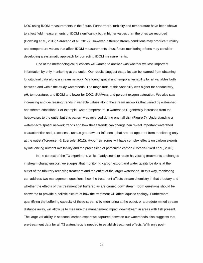
24

DOC using fDOM measurements in the future. Furthermore, turbidity and temperature have been shown

to affect field measurements of fDOM significantly but at higher values than the ones we recorded

(Downing et al., 2012; Saraceno et al., 2017). However, different stream conditions may produce turbidity

and temperature values that affect fDOM measurements; thus, future monitoring efforts may consider

developing a systematic approach for correcting fDOM measurements.

One of the methodological questions we wanted to answer was whether we lose important

information by only monitoring at the outlet. Our results suggest that a lot can be learned from obtaining

longitudinal data along a stream network. We found spatial and temporal variability for all variables both

between and within the study watersheds. The magnitude of this variability was higher for conductivity,

pH, temperature, and fDOM and lower for DOC, SUVA254, and percent oxygen saturation. We also saw

increasing and decreasing trends in variable values along the stream networks that varied by watershed

and stream conditions. For example, water temperature in watershed D generally increased from the

headwaters to the outlet but this pattern was reversed during one fall visit (Figure 7). Understanding a

watershed’s spatial network trends and how these trends can change can reveal important watershed

characteristics and processes, such as groundwater influence, that are not apparent from monitoring only

at the outlet (Torgersen & Ebersole, 2012). Hyporheic zones will have complex effects on carbon exports

by influencing nutrient availability and the processing of particulate carbon (Corson-Rikert et al., 2016).

In the context of the T3 experiment, which partly seeks to relate harvesting treatments to changes

in stream characteristics, we suggest that monitoring carbon export and water quality be done at the

outlet of the tributary receiving treatment and the outlet of the larger watershed. In this way, monitoring

can address two management questions: how the treatment affects stream chemistry in that tributary and

whether the effects of this treatment get buffered as are carried downstream. Both questions should be

answered to provide a holistic picture of how the treatment will affect aquatic ecology. Furthermore,

quantifying the buffering capacity of these streams by monitoring at the outlet, or a predetermined stream

distance away, will allow us to measure the management impact downstream in areas with fish present.

The large variability in seasonal carbon export we captured between our watersheds also suggests that

pre-treatment data for all T3 watersheds is needed to establish treatment effects. With only post-

25

treatment measurements, we will not be able to distinguish between the effects of climate, topology, and

harvesting treatment.

Our results also inform the temporal aspect of monitoring. We found precipitation to have a strong

effect on carbon quality and quantity, suggesting that monitoring efforts should follow precipitation

patterns. Tunaley et al. (2016) found that high DOC concentrations persisted after discharge returned to

baseflow during a rain event with warm, dry antecedent conditions in the Bruntland Burn catchment in NE

Scotland. Thus, monitoring during and after summer rain events could capture periods of high carbon

export. In the fall, wet antecedent conditions are more common and carbon export more closely follows

discharge patterns (Hood et al., 2006). Stream discharge responses to large amounts of precipitation are

flashy and temporally intensive monitoring is needed initially to capture the pattern of carbon flux.

Furthermore, studies have found seasonal patterns of hysteresis but the direction, whether clockwise

(Hood et al., 2006; Wilson et al., 2013) or counterclockwise (Strohmeier et al., 2013), of the relationship

between DOC concentration and discharge varies by study system. Storm event carbon dynamics should

be explored further in order to better understand the temporal patterns of carbon export and inform

monitoring practices.

Through the collection of more data in different climatic conditions and seasons, we can begin

developing a model for carbon export. Wilson et al. (2013) characterized seasonal changes in the DOC

concentration-discharge relationship through multiple power law relationships in Bigelow Brook, MA. To

develop a model with this kind of detail would require predicting DOC from fDOM and sampling

throughout the year. For Deer Creek, CO, Boyer et al. (1997) combined the hydrological model

TOPMODEL with carbon data to investigate hydrological mechanisms controlling DOC concentrations in

Deer Creek, CO. Development of future models will also need to explore the different spatial scales at

which DOC varies to better understand the dominant processes driving network patterns (McGuire et al.,

2014). Also, incorporating sorption-based soil models can give us a better estimate of the quantity and

composition of terrestrial carbon pools (Neff & Asner, 2001). Further quantifying the influences of

landscape and climatic drivers on carbon export in the Olympic Peninsula will best inform model

development.

Recommendations for Future Studies

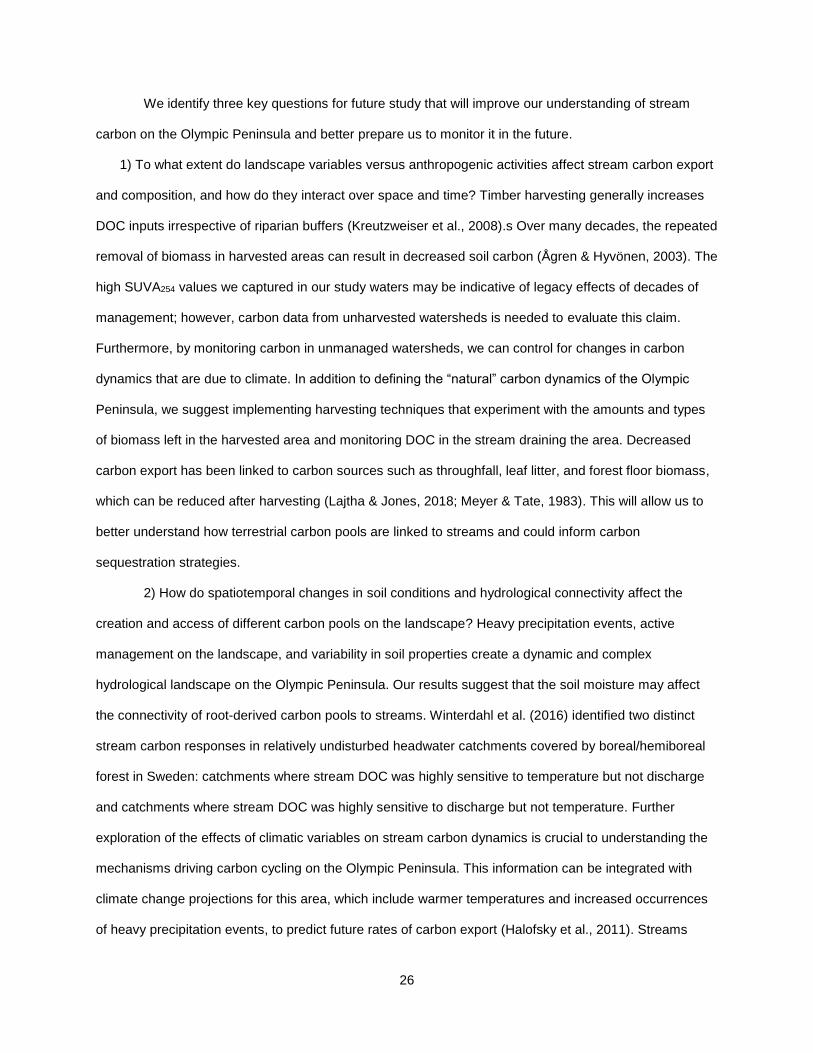
26

We identify three key questions for future study that will improve our understanding of stream

carbon on the Olympic Peninsula and better prepare us to monitor it in the future.

1) To what extent do landscape variables versus anthropogenic activities affect stream carbon export

and composition, and how do they interact over space and time? Timber harvesting generally increases

DOC inputs irrespective of riparian buffers (Kreutzweiser et al., 2008).s Over many decades, the repeated

removal of biomass in harvested areas can result in decreased soil carbon (Ågren & Hyvönen, 2003). The

high SUVA254 values we captured in our study waters may be indicative of legacy effects of decades of

management; however, carbon data from unharvested watersheds is needed to evaluate this claim.

Furthermore, by monitoring carbon in unmanaged watersheds, we can control for changes in carbon

dynamics that are due to climate. In addition to defining the “natural” carbon dynamics of the Olympic

Peninsula, we suggest implementing harvesting techniques that experiment with the amounts and types

of biomass left in the harvested area and monitoring DOC in the stream draining the area. Decreased

carbon export has been linked to carbon sources such as throughfall, leaf litter, and forest floor biomass,

which can be reduced after harvesting (Lajtha & Jones, 2018; Meyer & Tate, 1983). This will allow us to

better understand how terrestrial carbon pools are linked to streams and could inform carbon

sequestration strategies.

2) How do spatiotemporal changes in soil conditions and hydrological connectivity affect the

creation and access of different carbon pools on the landscape? Heavy precipitation events, active

management on the landscape, and variability in soil properties create a dynamic and complex

hydrological landscape on the Olympic Peninsula. Our results suggest that the soil moisture may affect

the connectivity of root-derived carbon pools to streams. Winterdahl et al. (2016) identified two distinct

stream carbon responses in relatively undisturbed headwater catchments covered by boreal/hemiboreal

forest in Sweden: catchments where stream DOC was highly sensitive to temperature but not discharge

and catchments where stream DOC was highly sensitive to discharge but not temperature. Further

exploration of the effects of climatic variables on stream carbon dynamics is crucial to understanding the

mechanisms driving carbon cycling on the Olympic Peninsula. This information can be integrated with

climate change projections for this area, which include warmer temperatures and increased occurrences

of heavy precipitation events, to predict future rates of carbon export (Halofsky et al., 2011). Streams

27

experiencing heavier rain events more often could not only increase their carbon export but could also

transport this carbon further downstream from the source, changing the distribution of nutrients for

aquatic biota (Raymond et al., 2016). Studies have found that increased soil temperatures raise the rates

of litter decay regardless of soil properties, resulting in faster terrestrial carbon losses (Ågren & Hyvönen,

2003; Gregorich et al., 2017). Changes in soil carbon induced by climate change will be reflected in the

streams, possibly resulting in profound changes to aquatic ecology.

3) How do spatiotemporal patterns of carbon on the landscape affect the availability and export of

other nutrients and vice versa? Carbon cycling is linked to processes that function at different spatial and

temporal scales. Chemical weathering, which is driven by plants and parent material composition,

generates multiple pathways through which acids, minerals, and metals are produced, broken down, and

exported (Keller, 2019). Carbon removal is driven in part by the formation of organo-mineral complexes

with Ca, Fe, and other weathered cations. This process of abiotic sorption is a primary pathway through

which carbon is incorporated into soil organic matter in Pacific Northwest forests (Yano et al., 2005).

Furthermore, increases in labile stream DOC result in increased stream metabolism and bacterial growth,

growing the assimilative demand for nitrogen (Bernhardt & Likens, 2002). The presence of nitrogen-fixing

alder in riparian areas has been found to have cascading effects on the surrounding vegetation,

availability of inorganic N, and characteristics of colored dissolved organic matter in the stream (Whigham

et al., 2017). Alder leaves also serve as a direct input of organic matter into the streams. Incorporating

these drivers and modifiers of the carbon cycle will allow us to contextualize carbon export within larger

landscape processes.

Conclusion

Our study provided a first look at carbon dynamics in small, fish-bearing streams on the Olympic

Peninsula. We found that carbon dynamics and water quality parameters were affected by complex

interactions between landscape characteristics and climatic conditions. We also identified two distinct

carbon pools on the landscape, though we did not have enough data to confirm the sources of these

compounds. Many more questions remain, but our results point to three directions of future study that will

inform key gaps in understanding carbon processes. By incorporating carbon-focused questions in

management experiments and exploring the interactions between nutrient cycles at multiple spatial and

28

temporal scales, we can build a conceptual framework that incorporates the effects of human

disturbance, landscape variability, and climate change. This framework can then be used to develop

carbon-conscious management strategies and to better prepare for a future climate.

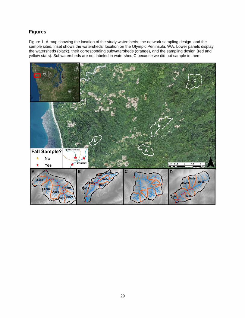
29

Figures Figure 1. A map showing the location of the study watersheds, the network sampling design, and the sample sites. Inset shows the watersheds’ location on the Olympic Peninsula, WA. Lower panels display the watersheds (black), their corresponding subwatersheds (orange), and the sampling design (red and yellow stars). Subwatersheds are not labeled in watershed C because we did not sample in them.

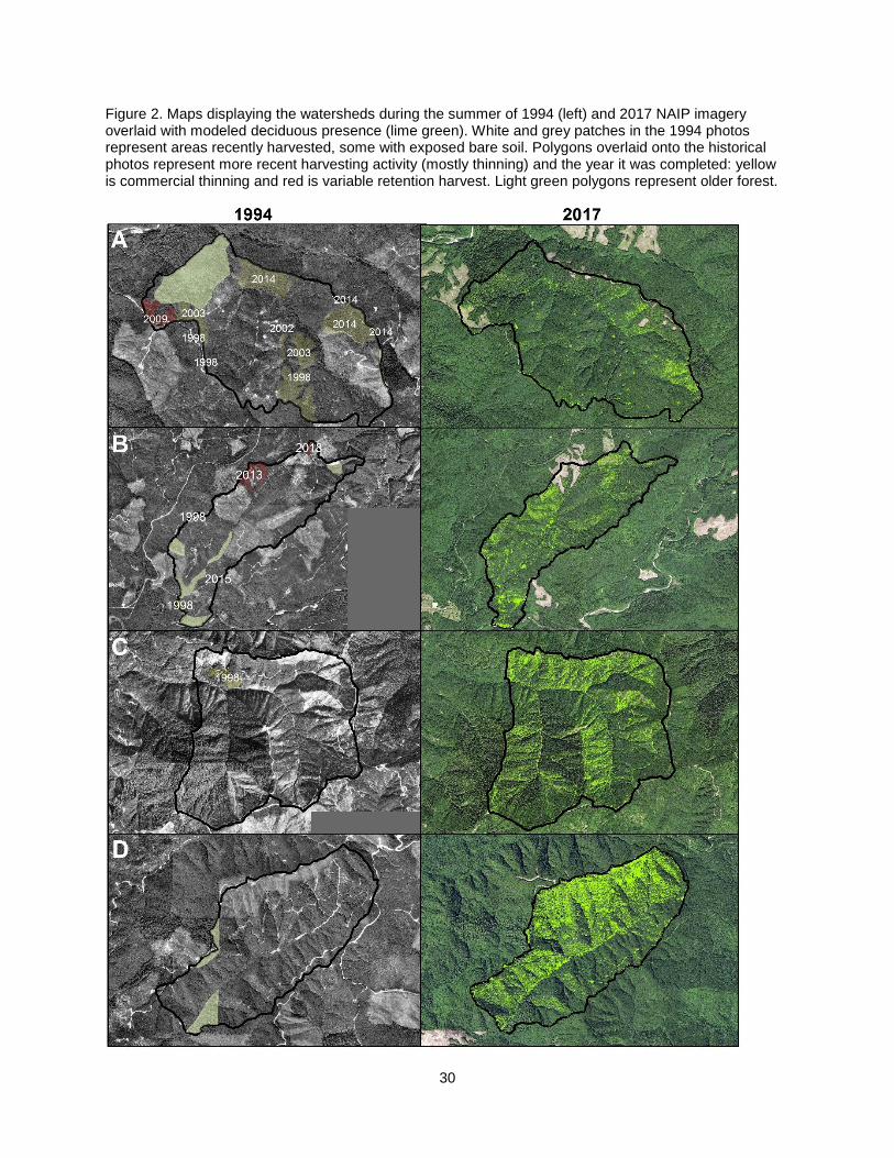
30

Figure 2. Maps displaying the watersheds during the summer of 1994 (left) and 2017 NAIP imagery overlaid with modeled deciduous presence (lime green). White and grey patches in the 1994 photos represent areas recently harvested, some with exposed bare soil. Polygons overlaid onto the historical photos represent more recent harvesting activity (mostly thinning) and the year it was completed: yellow is commercial thinning and red is variable retention harvest. Light green polygons represent older forest.

31

Figure 3. Maps of binned vegetation height classes in each watershed used for landscape metric analysis. Areas of old forest are delineated in yellow.

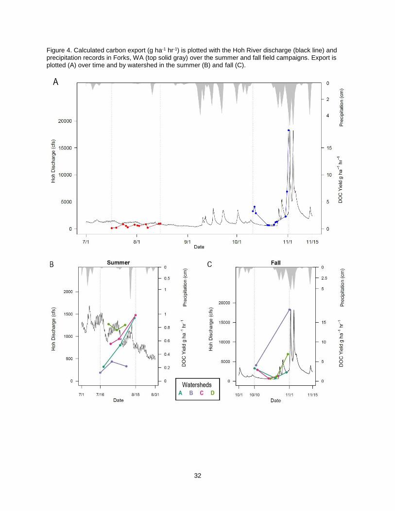
32

Figure 4. Calculated carbon export (g ha-1 hr-1) is plotted with the Hoh River discharge (black line) and precipitation records in Forks, WA (top solid gray) over the summer and fall field campaigns. Export is plotted (A) over time and by watershed in the summer (B) and fall (C).

33

Figure 5. Spatiotemporal patterns of conductivity (µS s-1) along the stream networks of the four study watersheds (A-D). Triangles represent values collected from sub-watershed streams. Yellow boxes represent summer and blue boxes represent fall. Sample point colors reflect different discharges (m3 hr-1

ha-1) measured at the outlet.

Figure 6. Spatiotemporal patterns of pH along the stream networks of the four study watersheds (A-D). Triangles represent values collected from sub-watershed streams. Yellow boxes represent summer and blue boxes represent fall. Sample point colors reflect different discharges (m3 hr-1 ha-1) measured at the outlet.

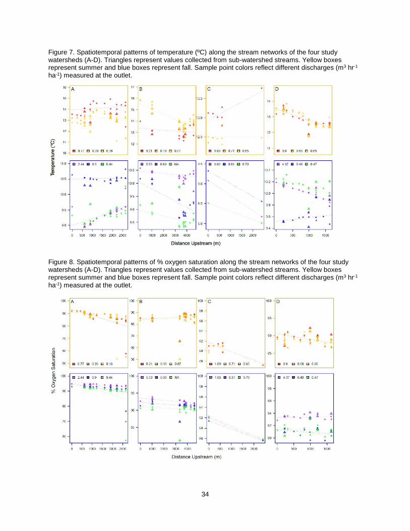
34

Figure 7. Spatiotemporal patterns of temperature (ºC) along the stream networks of the four study watersheds (A-D). Triangles represent values collected from sub-watershed streams. Yellow boxes represent summer and blue boxes represent fall. Sample point colors reflect different discharges (m3 hr-1


Figure 8. Spatiotemporal patterns of % oxygen saturation along the stream networks of the four study watersheds (A-D). Triangles represent values collected from sub-watershed streams. Yellow boxes represent summer and blue boxes represent fall. Sample point colors reflect different discharges (m3 hr-1


35

Figure 9. Spatiotemporal patterns of DOC (mg L-1) along the stream networks of the four study watersheds (A-D). Triangles represent values collected from sub-watershed streams. Yellow boxes represent summer and blue boxes represent fall. Sample point colors reflect different discharges (m3 hr-1


Figure 10. Spatiotemporal patterns of fDOM (RFU) along the stream networks of the four study watersheds (A-D). Triangles represent values collected from sub-watershed streams. Yellow boxes represent summer and blue boxes represent fall. Sample point colors reflect different discharges (m3 hr-1


36

Figure 11. Spatiotemporal patterns of SUVA254 (L mg-1 m-1) along the stream networks of the four study




37

Figure 12. Scatterplots, density plots, and correlation values for DOC (mg L-1), SUVA254 (L mg-1 m-1), and fDOM (RFU) from all sites. Colors represent the season the data point was collected.

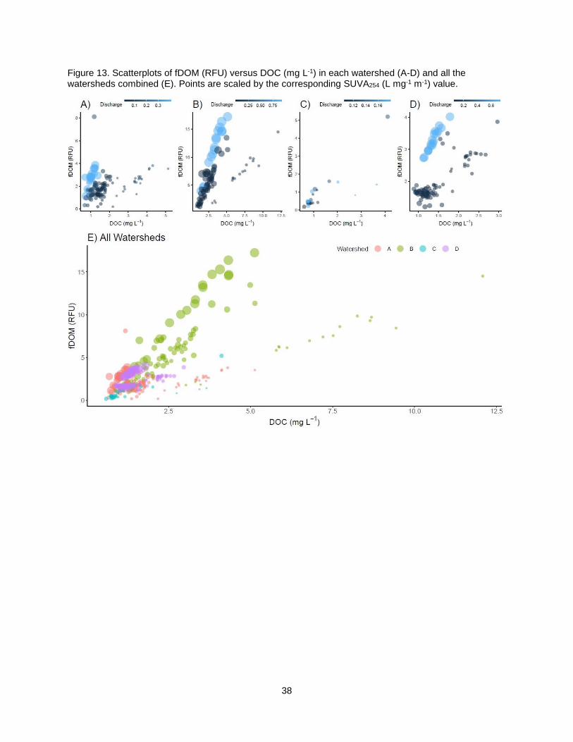
38

Figure 13. Scatterplots of fDOM (RFU) versus DOC (mg L-1) in each watershed (A-D) and all the watersheds combined (E). Points are scaled by the corresponding SUVA254 (L mg-1 m-1) value.

39

Figure 14. DOC (mg L-1) plotted with the most important variables identified by conditional random forest models. Seasonal linear regressions and the corresponding 95% confidence intervals (shaded areas) are also plotted with the R2 values reported in the legend. Points are scaled by the corresponding 3-day precipitation value.

Figure 15. fDOM (RFU) plotted with the most important variables identified by conditional random forest models. Seasonal linear regressions and the corresponding 95% confidence intervals (shaded areas) are also plotted with the R2 values reported in the legend. Points are scaled by the corresponding 1-day precipitation value.

40

Figure 16. SUVA (L mg-1 m-1) plotted with the most important variables identified by conditional random forest models. Seasonal linear regressions and the corresponding 95% confidence intervals (shaded areas) are also plotted with the R2 values reported in the legend. Points are scaled by the corresponding 3-day precipitation value.

41

Tables Table 1. Summary table of watershed and subwatershed descriptors. The number in parentheses under “Sample Sites” represents the number of sites sampled in the fall, if different from the summer.

Watershed Size (km2)

Elev. of Pour

Point (m)

Management Status

Recent Management

(% of Drainage Area)

Geology Sample

Sites Subwatershed

A 3.54 80

Commercial thinnings and

variable retention harvest (2009)

10.2 54% Glacial Drift 46% Greywacke

22 (20)

Aa01 0.47 103.9

Primarily old forest with 2009

variable retention harvest

17.3

Aa02 0.62 112.4 19.0 Aa03 0.47 143.3 19.2 Aa04 0.29 155.9 21.9 Aa05 0.22 178.5 22.8 Aa06 0.44 178.7 21.4

B 6.10 82.3

Patches of old forest and

variable retention harvest (2013)

7.7 95% Greywacke 5% Glacial Drift

16

Ba01 0.66 97.1 14.9 Ba02 0.13 178.9 25.0 Ba03 0.52 187.6 14.1 Ba04 0.91 191.4 10.8

Ba05 0.15 207.1 Variable

retention harvest (2013)

10.1

Ba06 1.14 207.1 10.7

C 6.05 263.6 Largest amount

of untouched forest

16.7 100% Greywacke 7 (2)

D 2.27 68.6 Small patches of untouched forest

near outlet 12.4 100% Glacial Drift 18

Da01 0.11 72.9 28.3 Da02 0.11 91.7 36.3 Da03 0.31 98.1 28.2 Da04 0.27 112.2 30.7 Da05 0.83 112.2 18.3

42

Table 2. Median and range values for climatic and landscape variables for all sites. Summer and fall (in parentheses) values are displayed for climatic variables. VH = Vegetation Height

CATEGORY VARIABLE DESCRIPTION MIN. MEDIAN MAX.

CLIMATE

1DayPrecip Amount of precipitation the day of

data collection; cm 0 (0) 0 (0)

1.4 (3.2)

3DayPrecip 3-day cumulative precipitation; cm 0 (0) 0 (0.7) 1.4

(4.6)

3DayDD50 3-day cumulative degree days

above 50º F 32.6 (1.4)

47.6 (4) 57

(15.5)

WATERSHED

Mean Slope % rise 19.1 52.1 76.0

Mean Stream Slope º 11.1 33.0 51.2

Mean Stream Elevation m 113.3 221.4 643.5

FWS Flow-weighted slope; % 7.7 14.9 36.3

ModeledUnstable % of drainage area that was

modeled unstable 0 44.5 66.8

ModeledDeciduous % of drainage area that was

modeled deciduous 1.3 6.8 35.5

Old Forest % of drainage area that is

unharvested forest 0 1.0 73.9

MeanVH Mean veg. height; m 9.8 19.4 25.7

StDevVH Veg. height standard deviation; m 4 8.5 14.4

MaxVH Maximum veg. height; m 33.8 63.4 85.6

SITE

Stream Substrate Boulders > 250 mm; % 0 15 50

Cobbles 75 – 250 mm; % 5 40 63

Gravel 2 – 64 mm; % 15 40 70

Fines < 2 mm; % 0 5 30

Bedrock % 0 0 50

Overstory ALRU A. rubra Bong.; % 0 60 90

PISI P. sitchensis (Bong.) Carriére; % 0 0 25

TSHE T. heterophylla (Raf.) Sarg.; % 0 30 95

THPL T. plicata Donn ex D. Don; % 0 0 35

ACCI A. circinatum Pursh; % 0 0 10

PSME P. menziesii (Mirb.) Franco; % 0 0 20

Open No canopy; % 0 0 50

Understory WoodyShrubs % of site 5 30 80 HerbsForbs % of site 2 30 60

Ferns % of site 1 10 30 Moss % of site 0 20 87

Grass % of site 0 1 30

Bare % of site 0 0 20

Bankfull Width Width of stream channel at

bankfull flow; m 0.9 4.0 7.4

FRAGSTATS

VH Largest Patch Index (VHLPI)

Area of largest patch divided by total landscape area; %

14.3 43.1 72.4

VH Edge Density (VHED) Sum of lengths of all edge segments divided by total landscape area; m ha-1

558 2308 3851

VH Contagion (VHCONTAG) Nears 0 when patch types are

maximally disaggregated and 100 when maximally aggregated; %

32.5 46.5 64.3

VH Patch Richness Density (VHPRD)

# of different patch types over total landscape area; # 100 ha-1 0.06 1.79 12.4

VH Shannon’s Evenness Index (VHSHEI)

Approaches 1 as distribution of area among patch types becomes

more even 0.45 0.75 0.93

43

Table 3. Watershed-scale landscape characteristic values and calculated FRAGSTATS metrics for each watershed.

VARIABLE WATERSHED

A B C D

Mean Slope (%) 51.4 40.6 73.8 62.2

Mean Stream Slope (º) 30.3 19.2 49.2 34.4

Mean Stream Elevation (m) 194.8 223.4 514.9 167.3

Flow-Weighted Slope (%) 10.2 7.7 16.7 12.4

Modeled Unstable (%) 45.8 12.4 37.1 55.8

Modeled Deciduous (%) 3.7 8.2 10.3 21.8

% Old Forest 11.6 7.5 27.2 4.4

Mean Vegetation Height (m) 22.4 18.9 18.7 20.1

St. Dev. Vegetation Height (m) 10.1 9.4 11.5 7.3

Max Vegetation Height (m) 84.2 82.7 85.8 74.8

VH Largest Patch Index (%) 43.3 27 43.4 47.2

VH Edge Density (m ha-1) 1,061.9 841 3,392.4 712.9

VH Contagion (%) 38.5 45.4 39.4 54.5

VH Patch Richness Density (# per 100 ha) 0.11 0.06 0.66 0.16

VH Shannon’s Evenness Index 0.85 0.78 0.84 0.64

Table 4. Median and range values for stream chemistry throughout summer and fall (parentheses). Starred variables were not used in data analysis due to data issues or correlation to other variables.

VARIABLE DESCRIPTION MIN. MEDIAN MAX. ST. DEV.

DOC mg L-1 0.60 (0.69) 1.25 (1.89) 5.1 (12.1) 0.67 (1.85) SUVA254 L mg-1 m-1 1.1 (0.85) 2.9 (2.7) 6.8 (7.8) 0.76 (2.07)

CONDUCTIVITY µS cm-1 0.66 (16) 42.7 (41) 84.4 (127.9) 14.8 (24.0) PH pH units 6.05 (5.9) 6.9 (6.9) 7.7 (7.6) 0.3 (0.31)

TEMPERATURE °C 11.1 (8) 13.3 (9.7) 15.9 (10.8) 0.8 (0.64) *TOTAL

DISSOLVED SOLIDS

mg L-1 0.64 (14.2) 36 (37.5) 71.1 (116) 12.6 (21.9)

FDOM Relative fluorescence

units (RFU) 0.18 (0.58) 1.64 (2.8) 11.3 (17.2) 2 (3.5)

*TURBIDITY Formazin

Nephelometric Unit (FNU)

0.49 (0.69) 1.3 (1.42) 1,195.8 (34.8)

155 (3.9)

OXYGEN SATURATION

% Saturation 50 (57.2) 88.1 (91.7) 92.2 (94.9) 6 (3.8)

*DISCHARGE m3 hr-1 ha-1 0.01 (0.07) 0.11 (0.11) 0.18 (0.91) 0.05 (0.29)

44

Table 5. Mean and standard deviation values (in parentheses) for each carbon and water quality variable collected at the outlet of each watershed during both seasons. Averages are based on three data points. Some water quality data is missing in the fall for watershed D due to equipment malfunctioning.

VARIABLE SEASON WATERSHED

A B C D

DOC (mg L-1) S 1.3 (0.1) 1.4 (0.3) 0.9 (0.1) 1.2 (0.1)

F 2.1 (1.1) 3.8 (1.9) 1.8 (0.9) 1.8 (0.6)

SUVA254 (L mg-1 m-1) S 2.9 (0.6) 3.0 (0.2) 2.3 (0.7) 3.4 (0.3)

F 2.9 (2.0) 4.2 (2.8) 1.9 (0.9) 3.9 (2.3)

fDOM (RFU) S 1.6 (0.5) 2.2 (0.3) 0.5 (0.1) 1.6 (<0.1)

F 2.1 (0.3) 7.2 (3.7) 1.0 (0.5) 3.3

Conductivity (µS cm-1) S 41.6 (2.5) 47.0 (2.8) 77.9 (5.5) 51.2 (1.5)

F 45.0 (17.6) 34.4 (8.2) 89.5 (29.0) 69.8

pH S 7.3 (0.1) 6.8 (0.2) 7.5 (>0.1) 7.0 (0.1)

F 7.1 (0.1) 6.8 (0.2) 7.6 (0.1) 6.9

Temperature (°C) S 13.2 (0.4) 15.2 (1.1) 12.7 (0.4) 13.4 (0.2)

F 9.9 (0.7) 10.0 (0.7) 9.0 (0.4) 10.2

Total Dissolved Solids (mg L-1)

S 35.0 (1.8) 37.5 (1.7) 66.1 (4.3) 42.9 (1.0)

F 41.3 (16.4) 31.7 (7.8) 83.7 (26.4) 63.3

Turbidity (FNU) S 0.5 (<<0.1) 1.2 (0.6) 0.8 (0.2) 1.2 (0.9)

F 0.9 (0.1) 2.1 (2.3) 0.8 (0.1) 1.8

% Oxygen Saturation S 91.5 (0.3) 84.1 (1.1) 90.2 (0.7) 89.2 (0.3)

F 93.6 (1.1) 91.5 (1.1) 91.9 (0.4) 92.0

45

Table 6. Measured discharge, DOC concentration, and calculated instantaneous carbon export for the study watersheds during the three summer (S) and three fall (F) visits. Export values could not be calculated for the second fall visit for watershed B due to missing discharge data.

Watershed Season Discharge

(m3 ha-1 hr-1) DOC

(mg L-1) Export

(g ha-1 hr-1)

A

S

0.16 1.35 0.21

0.39 1.37 0.53

0.77 1.22 0.94

F

0.90 3.64 3.27

0.44 1.75 0.77

2.44 0.93 2.26

B

S

0.07 1.74 0.12

0.21 1.36 0.29

0.19 1.14 0.22

F

0.70 5.87 4.07

NA 2.18 NA

5.53 3.30 18.25

C

S

0.71 0.78 0.55

0.65 0.96 0.63

1.09 0.90 0.98

F

1.06 2.75 2.90

0.79 0.88 0.70

0.81 1.65 1.33

D

S

0.68 1.25 0.85

0.66 1.16 0.76

0.80 1.04 0.84

F

0.48 1.36 0.65

0.47 2.56 1.19

4.37 1.58 6.88

46

Table 7. The R2 value, root mean square error (RMSE), and three most important variables (VI1-VI3) for each variable from seasonal (summer and fall) conditional reference random forest models. Variable importance values are reported in parentheses next to the variables. The color of the box represents the spatial scale of the predictor variable: blue = watershed, green = site, and yellow = climatic. We did not have enough variability in turbidity during the summer to run a model.

Variable Season R2 RMSE VI1 VI2 VI3

DOC S 0.60 0.44 MeanSlope (0.07) MeanStreamSlope

(0.04) ModeledUnstable

(0.01)

F 0.53 1.27 ModeledUnstable

(0.3) 3DayPrecip (0.3) MeanSlope (0.3)

SUVA254 S 0.42 0.58 MeanSlope (0.03) MeanStreamSlope

(0.02) Watershed (0.02)

F 0.88 0.71 3DayPrecip (3.0) 1DayPrecip (0.08) 3DayDD50 (0.05)

fDOM S 0.83 0.84 MeanSlope (2.6) PSME (0.1) ModeledDeciduous

(0.02)

F 0.85 1.42 MeanSlope (7.2) 1DayPrecip (0.4) MeanStreamSlope

(0.2)

pH S 0.77 0.15 MeanSlope (0.01) Watershed (0.01) Elevation (<0.01)

F 0.74 0.16 MeanSlope (0.04) 1DayPrecip

(<0.01) Watershed (<0.01)

Conductivity S 0.75 7.51 Watershed (28.1) Elevation (15.4) MeanStreamSlope

(11.9)

F 0.82 10.9 3DayPrecip

(190.6) Watershed (132.1) 1DayPrecip (51.1)

Temperature S 0.61 0.50 3DayDD50 (0.1) FWS (0.06) Moss (0.05)

F 0.78 0.31 3DayDD50 (0.12) Watershed (0.06) 1DayPrecip (0.05)

Turbidity F 0.13 2.29 VHSHEI (0.15) VHLPI (0.10) 1DayPrecip (0.1)

% Oxygen S 0.38 4.53 Gravel (1.19) MeanVH (1.14) Watershed (1.05)

F 0.33 3.35 3DayPrecip (0.80) Moss (0.44) MeanVH (0.43)

47

References

Abelho, M. (2001). From Litterfall to Breakdown in Streams: A Review. The Scientific World JOURNAL, 1, 656–680. https://doi.org/10.1100/tsw.2001.103

Ågren, G. I., & Hyvönen, R. (2003). Changes in carbon stores in Swedish forest soils due to increased biomass harvest and increased temperatures analysed with a semi-empirical model. Forest Ecology and Management, 174(1–3), 25–37. https://doi.org/10.1016/S0378-1127(02)00025-7

Aiken, G. R., Hsu-Kim, H., & Ryan, J. N. (2011). Influence of dissolved organic matter on the environmental fate of metals, nanoparticles, and colloids. Environmental Science and Technology, 45(8), 3196–3201. https://doi.org/10.1021/es103992s

Argerich, A., Haggerty, R., Johnson, S. L., Wondzell, S. M., Dosch, N., Corson-Rikert, H., … Thomas, C. K. (2016). Comprehensive multiyear carbon budget of a temperate headwater stream. Journal of Geophysical Research: Biogeosciences, 121(5), 1306–1315. https://doi.org/10.1002/2015JG003050

Arrigoni, A. S., Poole, G. C., Mertes, L. A. K., O’Daniel, S. J., Woessner, W. W., & Thomas, S. A. (2008). Buffered, lagged, or cooled? Disentangling hyporheic influences on temperature cycles in stream channels. Water Resources Research, 44(9), 1–13. https://doi.org/10.1029/2007WR006480

Ballard, T. M. (2000). Impacts of forest management on northern forest soils. Forest Ecology and Management, 133(1–2), 37–42. https://doi.org/10.1016/S0378-1127(99)00296-0

Barnes, R. T., Butman, D. E., Wilson, H. F., & Raymond, P. A. (2018). Riverine Export of Aged Carbon Driven by Flow Path Depth and Residence Time. Environmental Science and Technology, 52(3), 1028–1035. https://doi.org/10.1021/acs.est.7b04717

Battin, T. J. (1999). Hydrologic flow paths control dissolved organic carbon fluxes and metabolism in an Alpine stream hyporheic zone. Water Resources Research, 35(10), 3159–3169. https://doi.org/10.1029/1999WR900144

Bernhardt, E. S., & Likens, G. E. (2002). Dissolved Organic Carbon Enrichment Alters Nitrogen Dynamics in a Forest Stream. Ecological Society of America, 83(6), 1689–1700.

Bianchi, T. S., Garcia-Tigreros, F., Yvon-Lewis, S. A., Shields, M., Mills, H. J., Butman, D., … Grossman, E. L. (2013). Enhanced transfer of terrestrially derived carbon to the atmosphere in a flooding event. Geophysical Research Letters, 40(1), 116–122. https://doi.org/10.1029/2012GL054145

Bormann, B., & Minkova, T. (2017). OESF Large Scale Integrated Management Experiment (OESF T3 Experiment) Project Collaborative Workspace. Retrieved from http://www.onrc.washington.edu/ForestryPrograms/T3-OESF/

Boyer, E. W., Hornberger, G. M., Bencala, K. E., & McKnight, D. M. (1997). Response characteristics of DOC flushing in an alpine catchment. Hydrological Processes, 11(12), 1635–1647. https://doi.org/10.1002/(SICI)1099-1085(19971015)11:12<1635::AID-HYP494>3.0.CO;2-H

Breiman, L. (2001). Random Forests (Vol. 45).

Breiman, L., Friedman, J. H., Olshen, R. A., & Stone, C. J. (1984). Classification And Regression Trees. New York: Routledge. https://doi.org/10.1201/9781315139470

Burrows, R. M., Magierowski, R. H., Fellman, J. B., Clapcott, J. E., Munks, S. A., Roberts, S., … Barmuta, L. A. (2014). Variation in stream organic matter processing among years and benthic habitats in response to forest clearfelling. Forest Ecology and Management. https://doi.org/10.1016/j.foreco.2014.04.041

Butman, D., Stackpoole, S., Stets, E., McDonald, C. P., Clow, D. W., & Striegl, R. G. (2016). Aquatic carbon cycling in the conterminous United States and implications for terrestrial carbon accounting.

48

Proceedings of the National Academy of Sciences, 113(1), 58–63. https://doi.org/10.1073/pnas.1512651112

Corson-Rikert, H. A., Wondzell, S. M., Haggerty, R., & Santelmann, M. V. (2016). Carbon dynamics in the hyporheic zone of a headwater mountain stream in the Cascade Mountains, Oregon. Water Resources Research, 52(10), 7556–7576. https://doi.org/10.1002/2016WR019303

Creed, I. F., Sanford, S. E., Beall, F. D., Molot, L. A., & Dillon, P. J. (2003). Cryptic wetlands: Integrating hidden wetlands in regression models of the export of dissolved organic carbon from forested landscapes. Hydrological Processes, 17(18), 3629–3648. https://doi.org/10.1002/hyp.1357

Downing, B. D., Pellerin, B. A., Bergamaschi, B. A., Saraceno, J. F., & Kraus, T. E. C. (2012). Seeing the light: The effects of particles, dissolved materials, and temperature on in situ measurements of DOM fluorescence in rivers and streams. Limnology and Oceanography: Methods, 10(OCTOBER), 767–775. https://doi.org/10.4319/lom.2012.10.767

Dubayah, R. O., & Drake, J. B. (2000). Lidar Remote sensing for forestry applications. Journal of Forestry, 98(6), 44–46. https://doi.org/10.1093/jof/98.6.44

Fellman, J. B., Buma, B., Hood, E., Edwards, R. T., & D’Amore, D. V. (2017). Linking LiDAR with streamwater biogeochemistry in coastal temperate rainforest watersheds. Canadian Journal of Fisheries and Aquatic Sciences, 74(6), 801–811. https://doi.org/10.1139/cjfas-2016-0130

Fevold, K. L. (1998). Sub-surface controls on the distribution of benthic algae in floodplain back channel habitats of the Queets River. University of Washington, Seattle, WA.

Franklin, J. F., & Dyrness, C. T. (1988). Natural Vegetation of Oregon and Washington. Oregon State University Press. Retrieved from http://www.fsl.orst.edu/rna/Documents/publications/Natural vegetation of Oregon and Washington 1988.pdf

Gandy, C. J., Smith, J. W. N., & Jarvis, A. P. (2007). Attenuation of mining-derived pollutants in the hyporheic zone: A review. Science of The Total Environment, 373(2–3), 435–446. https://doi.org/10.1016/j.scitotenv.2006.11.004

Giese, L. A. B., Aust, W. M., Kolka, R. K., & Trettin, C. C. (2003). Biomass and carbon pools of disturbed riparian forests. Forest Ecology and Management, 180(1–3), 493–508. https://doi.org/10.1016/S0378-1127(02)00644-8

Gillooly, J. F., Brown, J. H., West, G. B., Savage, V. M., & Charnov, E. L. (2001). Effects of Size and Temperature on Metabolic Rate. Science, 293(5538), 2248–2251. https://doi.org/10.1126/science.1061967

Gray, A. N., Whittier, T. R., & Harmon, M. E. (2016). Carbon stocks and accumulation rates in Pacific Northwest forests: Role of stand age, plant community, and productivity. Ecosphere, 7(1), 1–19. https://doi.org/10.1002/ecs2.1224

Grayston, S. J., Vaughan, D., & Jones, D. (1996). Rhizosphere carbon flow in trees, in comparison with annual plants: the importance of root exudation and its impact on microbial activity and nutrient availability. Applied Soil Ecology (Vol. 5).

Gregorich, E. G., Janzen, H., Ellert, B. H., Helgason, B. L., Qian, B., Zebarth, B. J., … Dyck, M. F. (2017). Litter decay controlled by temperature, not soil properties, affecting future soil carbon. Global Change Biology, 23(4), 1725–1734. https://doi.org/10.1111/gcb.13502

Halofsky, J. E., Peterson, D. L., O’Halloran, K. A., & Hawkins Hoffman, C. (2011). Adapting to Climate Change at Olympic National Forest and Olympic National Park. Portland, OR. https://doi.org/NPW-GT-844

Halpern, C. B., & Spies, T. A. (1995). Plant Species Diversity in Natural and Managed Forests of the Pacific Northwest. Ecological Applications, 5(4), 913–934. https://doi.org/10.2307/2269343

49

Hijmans, R. J., & Ghosh, A. (2019). Spatial Data Analysis with R.

Hood, E., Gooseff, M. N., & Johnson, S. L. (2006). Changes in the character of stream water dissolved organic carbon during flushing in three small watersheds, Oregon. Journal of Geophysical Research: Biogeosciences, 111(1), 1–8. https://doi.org/10.1029/2005JG000082

Inamdar, S., Singh, S., Dutta, S., Levia, D., Mitchell, M., Scott, D., … McHale, P. (2011). Fluorescence characteristics and sources of dissolved organic matter for stream water during storm events in a forested mid-Atlantic watershed. Journal of Geophysical Research: Biogeosciences. https://doi.org/10.1029/2011JG001735

Jencso, K. G., McGlynn, B. L., Gooseff, M. N., Wondzell, S. M., Bencala, K. E., & Marshall, L. A. (2009). Hydrologic connectivity between landscapes and streams: Transferring reach- and plot-scale understanding to the catchment scale. Water Resources Research, 45(4). https://doi.org/10.1029/2008WR007225

Keller, C. K. (2019). Carbon Exports from Terrestrial Ecosystems: A Critical-Zone Framework. Ecosystems. https://doi.org/10.1007/s10021-019-00375-9

King, R. S., Baker, M. E., Whigham, D. F., Weller, D. E., Jordan, T. E., Kazyak, P. F., & Hurd, M. K. (2005). Spatial Considerations for Linking Watershed Land Cover to Ecological Indicators in Streams. Ecological Applications (Vol. 15).

Knapp, N., Fischer, R., & Huth, A. (2018). Linking lidar and forest modeling to assess biomass estimation across scales and disturbance states. Remote Sensing of Environment, 205(November 2017), 199–209. https://doi.org/10.1016/j.rse.2017.11.018

Kreutzweiser, D. P., Hazlett, P. W., & Gunn, J. M. (2008). Logging impacts on the biogeochemistry of boreal forest soils and nutrient export to aquatic systems: A review. Environmental Reviews, 16(NA), 157–179. https://doi.org/10.1139/A08-006

Lajtha, K., & Jones, J. (2018). Forest harvest legacies control dissolved organic carbon export in small watersheds, western Oregon. Biogeochemistry. https://doi.org/10.1007/s10533-018-0493-3

Lal, R. (2003). Soil erosion and the global carbon budget. Environment International. Elsevier Ltd. https://doi.org/10.1016/S0160-4120(02)00192-7

Laudon, H., Berggren, M., Ågren, A., Buffam, I., Bishop, K., Grabs, T., … Köhler, S. (2011). Patterns and Dynamics of Dissolved Organic Carbon (DOC) in Boreal Streams: The Role of Processes, Connectivity, and Scaling. Ecosystems, 14(6), 880–893. https://doi.org/10.1007/s10021-011-9452-8

Mcdowell, W. H., & Fisher, S. G. (1976). Autumnal Processing of Dissolved Organic Matter in a Small Woodland Stream Ecosystem (Vol. 57).

McGarigal, K., & Marks, B. J. (1995). FRAGSTATS: spatial pattern analysis program for quantifying landscape structure. Portland, OR. https://doi.org/10.2737/PNW-GTR-351

McGuire, K. J., Torgersen, C. E., Likens, G. E., Buso, D. C., Lowe, W. H., & Bailey, S. W. (2014). Network analysis reveals multiscale controls on streamwater chemistry. Proceedings of the National Academy of Sciences, 111(19), 7030–7035. https://doi.org/10.1073/pnas.1404820111

Means, J. E., Acker, S. A., Fitt, B. J., Renslow, M., Emerson, L., & Hendrix, C. J. (2000). Predicting forest stand characteristics with airborne scanning lidar. Photogrammetric Engineering & Remote Sensing, 66(11), 1367–1371.

Melson, S. L., Harmon, M. E., Fried, J. S., & Domingo, J. B. (2011). Estimates of live-tree carbon stores in the Pacific Northwest are sensitive to model selection. Carbon Balance and Management, 6. https://doi.org/10.1186/1750-0680-6-2

Meyer, J. L., & Tate, C. M. (1983). The Effects of Watershed Disturbance on Dissolved Organic Carbon Dynamics of a Stream. Ecology, 64(1), 33–44.

50

Minkova, T., & Devine, W. (2016). Status and Trends Monitoring of Riparian and Aquatic Habitat in the Olympic Experimental State Forest: Habitat Status Report and 2015 Project Progress Report. Olympia, WA.

Monteith, D. T., Stoddard, J. L., Evans, C. D., De Wit, H. A., Forsius, M., Høgåsen, T., … Vesely, J. (2007). Dissolved organic carbon trends resulting from changes in atmospheric deposition chemistry. Nature, 450(7169), 537–540. https://doi.org/10.1038/nature06316

Moore, R. D., & Wondzell, S. M. (2005). Physical Hydrology and the Effects of Forest Harvesting in the Pacific Northwest: A Review. Journal of the American Water Resources Association, 41(4), 763–784.

Mosher, J. J., Kaplan, L. A., Podgorski, D. C., Mckenna, A. M., & Marshall, A. G. (2015). Longitudinal shifts in dissolved organic matter chemogeography and chemodiversity within headwater streams: a river continuum reprise, 124(1), 371–385. https://doi.org/10.1007/s

Mulholland, P. J., & Hill, W. R. (1997). Seasonal patterns in streamwater nutrient and dissolved organic carbon concentrations: Separating catchment flow path and in-stream effects. Water Resources Research, 33(6), 1297–1306. https://doi.org/10.1029/97WR00490

Mulholland, P. J., Marzolf, E. R., Webster, J. R., Hart, D. R., & Hendricks, S. P. (1997). Evidence that hyporheic zones increase heterotrophic metabolism and phosphorus uptake in forest streams. Limnology and Oceanography, 42(3), 443–451.

Neff, J. C., & Asner, G. P. (2001). Dissolved organic carbon in terrestrial ecosystems: Synthesis and a model. Ecosystems, 4(1), 29–48. https://doi.org/10.1007/s100210000058

Olden, J. D., Lawler, J. J., & Poff, N. L. (2008). Machine Learning Methods Without Tears: A Primer for Ecologists. The Quarterly Review of Biology. https://doi.org/10.1086/587826

Oliver, A. A., Tank, S. E., Giesbrecht, I., Korver, M. C., Floyd, W. C., Sanborn, P., … Lertzman, K. P. (2017). Globally significant yields of dissolved organic carbon from small watersheds of the Pacific coastal temperate rainforest. Biogeosciences Discussions, (January), 1–44. https://doi.org/10.5194/bg-2017-5

Prairie, Y. T. (2008). Carbocentric limnology: looking back, looking forward. Canadian Journal of Fisheries and Aquatic Sciences, 65(3), 543–548. https://doi.org/10.1139/f08-011

Prescott, C. E., Zabek, L. M., Staley, C. L., & Kabzems, R. (2000). Decomposition of broadleaf and needle litter in forests of British Columbia: influences of litter type, forest type, and litter mixtures. Canadian Journal of Forest Research, 30(11), 1742–1750. https://doi.org/10.1139/x00-097

R Core Team. (2018). R: A language and environment for statistical computing. Vienna, Austria: R Foundation for Statistical Computing. https://doi.org/https://www.R-project.org/

Raymond, P. A., Saiers, J. E., & Sobczak, W. V. (2016). Hydrological and biogeochemical controls on watershed dissolved organic matter transport: Pulse- shunt concept. Ecology, 97(1), 5–16. https://doi.org/10.1890/14-1684.1

Saraceno, J. F., Shanley, J. B., Downing, B. D., & Pellerin, B. A. (2017). Clearing the waters: Evaluating the need for site-specific field fluorescence corrections based on turbidity measurements. Limnology and Oceanography: Methods, 15(4), 408–416. https://doi.org/10.1002/lom3.10175

Sardá-Espinosa, A., Subbiah, S., & Bartz-Beielstein, T. (2017). Conditional inference trees for knowledge extraction from motor health condition data. Engineering Applications of Artificial Intelligence, 62, 26–37. https://doi.org/10.1016/j.engappai.2017.03.008

Schindler, J. E., & Krabbenhoft, D. P. (1998). The Hyporheic Zone as a Source of Dissolved Organic Carbon and Carbon Gases to a Temperate Forested Stream. Biogeochemistry, 43(2), 157–174.

Solinger, S., Park, J.-H., Michalzik, B., & Matzner, E. (2000). Controls on the dynamics of dissolved

51

organic matter in soils: a review [ Soils Issues ]. Soil Science, 165(April), 277–304.

Stanley, E. H., Powers, S. M., Lottig, N. R., Buffam, I., & Crawford, J. T. (2012). Contemporary changes in dissolved organic carbon (DOC) in human-dominated rivers: Is there a role for DOC management? Freshwater Biology, 57(SUPPL. 1), 26–42. https://doi.org/10.1111/j.1365-2427.2011.02613.x

Steinberg, C. E. W., Kamara, S., Prokhotskaya, V. Y., Manusadžianas, L., Karasyova, T. A., Timofeyev, M. A., … Menzel, R. (2006, July). Dissolved humic substances - Ecological driving forces from the individual to the ecosystem level? Freshwater Biology. https://doi.org/10.1111/j.1365-2427.2006.01571.x

Strohmeier, S., Knorr, K. H., Reichert, M., Frei, S., Fleckenstein, J. H., Peiffer, S., & Matzner, E. (2013). Concentrations and fluxes of dissolved organic carbon in runoff from a forested catchment: Insights from high frequency measurements. Biogeosciences, 10(2), 905–916. https://doi.org/10.5194/bg-10-905-2013

Sun, O. J., Campbell, J., Law, B. E., & Wolf, V. (2004). Dynamics of carbon stocks in soils and detritus across chronosequences of different forest types in the Pacific Northwest, USA. Global Change Biology, 10(9), 1470–1481. https://doi.org/10.1111/j.1365-2486.2004.00829.x

Thomas, J. D. (1997). The role of dissolved organic matter, particularly free amino acids and humic substances, in freshwater ecosystems. Freshwater Biology, 38(1), 1–36. https://doi.org/10.1046/j.1365-2427.1997.00206.x

Torgersen, C., & Ebersole, J. (2012). Primer for identifying cold-water refuges to protect and restore thermal diversity in riverine landscapes. EPA Scientific Guidance Handbook, (February), 91. https://doi.org/EPA 910-c-12-001

Tunaley, C., Tetzlaff, D., Lessels, J., & Soulsby, C. (2016). Linking high-frequency DOC dynamics to the age of connected water sources. Water Resources Research. https://doi.org/10.1002/2015WR018419

U.S. Climate Data. (2019). Retrieved from https://www.usclimatedata.com/

USEPA. (2010). EPA Drinking Water Guidance on Disinfection By-Products Advice Note No. 4. Version 2. Disinfection By-Products in Drinking Water. Environmental Protection Agency Office of Envrionmental Enforcement.

Walker, C. M., King, R. S., Whigham, D. F., & Baird, S. J. (2012). Landscape and wetland influences on headwater stream chemistry in the Kenai Lowlands, Alaska. Wetlands. https://doi.org/10.1007/s13157-011-0260-x

Waring, R. H., & Franklin, J. F. (1979). Evergreen Coniferous Forests of the Pacific Northwest. Science, 204(4400), 1380–1386.

Washington State Department of Natural Resources. (1997). Habitat Conservation Plan. Olympia, WA.

Washington State Department of Natural Resources. (2016). Forest Land Plan for the Olympic Experimental State Forest. Olympia, WA.

Wegmann, K. W., & Pazzaglia, F. J. (2002). Holocene strath terraces, climate change, and active tectonics: The Clearwater River basin, Olympic Peninsula, Washington State. Bulletin of the Geological Society of America, 114(6), 731–744. https://doi.org/10.1130/0016-7606(2002)114<0731:HSTCCA>2.0.CO;2

Weishaar, J. L., Aiken, G. R., Bergamaschi, B. A., Fram, M. S., Fujii, R., & Mopper, K. (2003). Evaluation of specific ultraviolet absorbance as an indicator of the chemical composition and reactivity of dissolved organic carbon. Environmental Science and Technology. https://doi.org/10.1021/es030360x

Wetzel, R. G. (2001). Limnology: Lake and River Ecosystems. Journal of Phycology (3rd ed., Vol. 37).

52

San Diego, CA: Academic Press.

Whigham, D. F., Walker, C. M., Maurer, J., King, R. S., Hauser, W., Baird, S., … Neale, P. J. (2017). Watershed influences on the structure and function of riparian wetlands associated with headwater streams – Kenai Peninsula, Alaska. Science of the Total Environment, 599–600, 124–134. https://doi.org/10.1016/j.scitotenv.2017.03.290

Wilson, H. F., Saiers, J. E., Raymond, P. A., & Sobczak, W. V. (2013). Hydrologic Drivers and Seasonality of Dissolved Organic Carbon Concentration, Nitrogen Content, Bioavailability, and Export in a Forested New England Stream. Ecosystems. https://doi.org/10.1007/s10021-013-9635-6

Winterdahl, M., Laudon, H., Lyon, S. W., Pers, C., & Bishop, K. (2016). Sensitivity of stream dissolved organic carbon to temperature and discharge: Implications of future climates. Journal of Geophysical Research: Biogeosciences, 121(1), 126–144. https://doi.org/10.1002/2015JG002922

Wohl, E., Hall, R. O., Lininger, K. B., Sutfin, N. A., & Walters, D. M. (2017). Carbon dynamics of river corridors and the effects of human alterations. Ecological Monographs, 87(3), 379–409. https://doi.org/10.1002/ecm.1261

Yano, Y., Lajtha, K., Sollins, P., & Caldwell, B. A. (2005). Chemistry and dynamics of dissolved organic matter in a temperate coniferous forest on andic soils: Effects of litter quality. Ecosystems, 8(3), 286–300. https://doi.org/10.1007/s10021-005-0022-9

53

Acknowledgements

This project would not have been possible without the contributions of many people. I would first

like to thank my incredibly talented committee for supporting my ideas and helping me grow as a scientist.

Thank you to my committee chair, Bernard Bormann, for giving me the freedom and financial support to

develop my own project and teaching me how to balance scientific curiosity with practical applicability. I

am also thankful to Teodora (Teddy) Minkova for her sharp insights, sincere enthusiasm, and enduring

patience in exploring steep terrain with me. I am deeply grateful to David Butman for sharing his lab

space and resources, contributing his expertise throughout the project, and challenging me intellectually. I

would also like to thank everyone who provided support for this project from the UW and SEFS

communities. Linda Stonehocker, Theresa Santman, Deric Kettel, Frank Hanson, and other staff at the

Olympic Natural Resources Center were invaluable in assisting with logistics, ensuring our safety, and

making us feel at home on the Peninsula. I would not have survived my summer field season without the

endless supply of positivity and energy from my intrepid field interns: Lily Allred, Kari Jessett, Thuy Luu,

Chloe May, and Esaac Mazengia. Thank you to Warren Devine (WADNR), Keven Bennett (UW), and

other DNR staff who kindly shared their work with me and patiently responded to my many emails.

Christian Torgersen (UW and USGS) supported the project by offering key insights into the data analysis

process. Thank you to Paul Heffner for his positive attitude during fall field work and completing some of

the initial exploratory analyses of the data. Courtney Bobsin was a supportive field partner and thoughtful

lab mate. Many thanks to Jason James and Catherine Kuhn for taking the time to explain scientific

protocols, sampling methods, and how to use lab machinery. Thank you to the Butman Lab for financially

supporting my analyses in the UW CEE Environmental Engineering Analytical Center and to J. Sean

Yeung for advising the use of the machines. Finally, I am indebted to my friends and family for their acts

of kindness, words of encouragement, and occasional reality checks that kept me sane throughout these

past two years.