liner shipping economics - harbour agency · pdf fileliner shipping economics j.o. jansson...
TRANSCRIPT
Liner Shipping Economics
Liner Shipping Economics J.O. Jansson Swedish Road and Traffic Research Institute Linkoping
and
D. Shneerson Department of Economics University of Haifa
London New York CHAPMAN AND HALL
First published in 1987 by Chapman and Hall Ltd 11 New Fetter Lane, London EC4P4EE Published in the USA by Chapman and Hall 29 West 35th Street, New York NYlO001
© 1987 J.O. Jansson and D. Shneerson
Softcover reprint of the hardcover 1st edition 1987
All rights reserved. No part of this book may be reprinted, or reproduced or utilized in any form or by any electronic, mechanical or other means, now known or hereafter invented, including photocopying and recording, or in any iriformation storage and retrieval system, without permission in writing from the publisher.
British Library Cataloguing in Publication Data
Jansson, Jan Owen Liner shipping economics. I. Shipping 2. Ocean liners I. Title II. Shneerson, Dan 387.5'1 HE593
ISBN-13: 978-94-010-7914-3
Library of Congress Cataloging in Publication Data
Jansson, Jan Owen. Liner shipping economics.
Bibliography: p. Includes index. l. Shipping. 2. Shipping-Rates. 3. Shipping conferences.
I. Shneerson, Dan. II. Title. HE582.J36 1987 387.5'1 86-20718
ISBN-13: 978-94-010-7914-3 DOl: 10.1007/978-94-009-3147-3
e-ISBN-13: 978-94-009-3147-3
Contents
Preface ix
PART I THE LINER SHIPPING INDUSTRY 1
1 Characteristics of demand and supply of liner shipping 3 1.1 An aggregate picture of seaborne trade and the world fleet
tonnage 3 1.2 The development of the shares of the world fleet: developed
countries, flags of convenience and developing countries 7 1.3 Liner shipping, shipping for hire and 'own shipping' 15 1.4 The relative size of the liner shipping industry 22 1.5 Recent development in general cargo shipping 22 1.6 Geographical aspects of liner shipping 30
2 Market organization: the conference system 35 2.l The scope of the conference system 35 2.2 Conference organization and main activities 35 2.3 Why conferences? 42 2.4 Concluding remarks 47
3 The level and structure of freight rates 49 3.1 The general level of freight rates 49 3.2 The structure of freight rates 66 Appendix A: The construction of the CON/SCaN index (1975-85) 84 Appendix B: The liner index of the FRG (1976-85) 88 Appendix C: The construction of an individual line freight rate index 89
4 The art of charging what the traffic can bear 94 4.1 The main form of price discrimination in liner shipping 94 4.2 The role of commodity value for shipping demand elasticity 95 4.3 The role of competition from other sources of goods supply for
shipping demand elasticity 100 4.4 Competition from 'outsiders' and other modes of transport 107 4.5 Summary and conclusions 107
PART II LINER SERVICE OPTIMIZATION 111
5 Ship size and shipping costs 113 5.1 Sizes of ships of different categories: The statistical picture 113

vi Contents
5.2 Plant-size economies in general 5.3 The three ship capacities 5.4 The model 5.5 Estimation of ship size elasticities of handling and hauling
capacities and factor costs 5.6 Economies of size at sea - diseconomies of size in port 5.7 Optimal ship size 5.8 Analysis of the effect on optimal ship size of parameter changes
in the model 5.9 The optimal size of a palletized reefer ship: A case study 5.10 Towards a model of ship size growth
6 Multi-port calling versus trans-shipment 6.1 The general problem: Feeder-transport cost minimization in a
given service range 6.2 The specific problem: The potential of sea-feeder transport 6.3 The very large container carriers and feeder services
7 Shippers' costs of sailings infrequency and transit time 7.1 Storage costs 7.2 Costs of sailings infrequency and transit time for goods which are
not stored by importers 7.3 Loss of value of perishable goods 7.4 How important are shippers' costs? Appendix: Optimal ship size when both shipping company
costs and the shippers' costs are accounted for
8 Port costs and charges and the problem of shipping and port sub-optimizations
8.1 'Public' general cargo transport systems versus 'private' bulk cargo transport systems
8.2 Bottlenecks in ports 8.3 Port charges as a means of coordinating shipping and port
operations
9 A cost minimization model of a liner trade 9.1 A liner trade model - purpose, scope and assumption 9.2 Total producer and user costs 9.3 Optimal ship size, multi-port diversion, and frequency of sailings 9.4 The minimum total cost per ton
PART III ECONOMIC EVALUATION OF THE CONFERENCE SYSTEM
10 The charging floor reconsidered 10.1 Economies of scale?
115 117 117
123 135 138
139 147 149
157
157 157 171
173 173
183 183 184
188
193
193 194
200
205 205 207 211 213
217
219 219
Contents vii
10.2 Common cost and factor indivisibility 223 Appendix: Model of profit-maximizing freight rate making 225
11 The freight rate structure is out of line with the marginal cost structure 238
11.1 Principles of marginal cost-based tariffs 238 11.2 Cross-subsidization between commodities 239 11.3 Excessive averaging of freight rates: Some suggestions for
reforming the tariff construction 242 11.4 Further aspects of a cost-based freight rate structure 247 Appendix: Freight rates and shipping marginal costs
of Israeli imports and exports 254
12 Potential cartel profits become social costs 264 12.1 Empirical evidence of low load factors in liner shipping 264 12.2 Model of supply and demand equilibrium in a liner trade 265 12.3 Some evidence of a negative relationship between the load factor
and the profit potential 273 12.4 Excessive service competition 275
13 Conclusion: price competition in liner shipping should be encouraged
13.1 The two types of ill effects 13.2 Allocative inefficiency effects 13.3 'Slack' effects 13.4 Encourage price competition and service coordination 13.5 Recent attempts of reforming liner conference practices 13.6 Problems of regulating international liner shipping 13.7 Hopes for the future
References
Author index
Subject index
276 276 277 280 281 285 286 287
289
293
295
Preface
The importance of international liner shipping needs little emphasizing. A large majority of international trade moves by sea, and the liner shipping share in total freight revenue exceeds one-half. Notwithstanding, people in general know surprisingly little about the basic facts of the liner shipping industry, and, in particular, about the economics ofliner shipping. Perhaps because it is an international industry, where shipping lines flying many different flags participate, it has tended to fall in between national accounts of domestic industries. Even transport economists have, generally speaking, treated liner shipping rather 'stepmotherly'; besides the work of Bennathan and Walters (1969), a relatively small group of specialized maritime economists, including A. Stromme-Svendsen, T. Thorburn, S. Sturmey, R. Goss, and B.M. Deakin, have in the post-war period made important contributions to the subject, but so far no coherent and reasonably comprehensive treatise of liner shipping economics has appeared. The first purpose of the present volume is therefore obvious: to provide just that.
The book is divided in three parts: Part I The liner shipping industry; Part II Liner service optimization; Part III Economic evaluation of the conference system. Needless to say, all three parts concur to fulfill the first purpose of providing a complete book of liner shipping economics. In Part II a more or less separate, second, purpose has been to develop analytical tools for liner service optimization.
Thereby we use different approaches. First we develop general models of, for example, ship-size optimization, the choice between multi-port calling and trans-shipment, etc. so far as it is fruitful to generalize. Then the general principles derived are illustrated by case studies or practical examples, which hopefully serve the double purpose of (i) conveying to the reader something of the reality of seaborne freight transport, as well as (ii) demonstrating the usefulness of sound theoretical underpinning of empirical studies of liner shipping operations.
A third purpose is to make substantial contribution to the long controversy over the omnipresent price cartels in liner shipping known as liner conferences. This is a very complex and difficult issue, especially in the present period of thorough structural change in liner shipping both technologically and organizationally, which could be sufficient for a whole book - the most recent example is Sletmo and Williams (1981). The present discussion of this longstanding issue is a natural continuation of the general economic analysis of the liner shipping industry in Parts I and II. The main stumbling block is, and has always been, misleading conceptions of the pricing-relevant marginal cost of scheduled transport services. A good century of administered liner freight rates
x Preface
has left costing principles in liner shipping lagging. We suggest various improvements in this field, but realize that the only certain way of exposing costing deficiencies is by freer pricing. Encouragement of price competition does not necessarily mean that all liner conferences have to be dissolved, but rather a change of object ofthe conferences from price fixing to coordination of sailings (schedules), ports of call and feeder services.
Writing this book, we have accumulated debts to many people, not the least to our families. Going back to where it started, our interest in the subject was awakened by working with Professors Thorburn, Walters, and Bannathan; later, contacts with friendly people from the shipping and port industries have been an invaluable factor of production. Informants are too many to mention individually, however, Nachum Gonzarsky of Zim Lines read chapters 1 and 2 and made valuable comments, for which we are grateful, and Y osi Sela of Zim assisted in the construction of the liner freight-rate indices. Shlomit ErgonKarlin devoted a lot of her time to the empirical work of chapters 1,5 and 9 and helped in the organization of the whole manuscript, which we gratefully acknowledge.
Many thanks to the EI-Yam Chair for Shipping and Ports which has generously financed the project in the final stages.
Haifa. October 1985 Jan Owen Jansson Dan Shneerson
PART THE LINER SHIPPING INDUSTRY ONE
In this part we describe the liner shipping industry from different points of view. In chapter 1 we take up some important characteristics of demand and supply of liner shipping including the types of cargo, ships, and trade routes involved. In chapter 2 the very specific market organization is described.
Practically all international liner shipping is organized as routespecific price cartels known as liner conferences. The conference system has existed for more than a century, and naturally has been subject to much discussion, but comparatively little regulatory action. We give a short historical background (see also Deakin, 1973), and outline recent tendencies in national as well as international shipping policy.
In chapters 3 and 4 the intriguing matter of freight rate making in liner shipping is dealt with. In chapter 3 the existing level and structure of freight rates are surveyed, and a hypothesis of ratemaking behaviour - charging what the traffic can bear over and above the direct handling costs - is tested statistically. Chapter 4 develops some ideas of improving the state of the art of freight rate making by combining derived-demand theory with the relevant facts of liner shipping markets.

1 Characteristics of demand and supply of liner shipping
The pattern of seaborne trade and shipping is determined by a multitude of factors, economic, geographic and political. In this chapter we have selected some factors of general importance as well as some factors of specific importance for the purpose of this book. The chapter starts by an aggregate picture, in which the liner shipping sector will gradually be identified from different points of view.
A short historical background is given and the current tendencies of the development of liner shipping are pointed out. The statistical data presented are compiled from the standard sources of currently published shipping statistics, if no other source is given. *
1.1 AN AGGREGATE PICTURE OF SEABORNE TRADE AND THE WORLD FLEET TONNAGE
Nations trade in order to increase their wealth. The role of international transport is to bridge the spatial separation of trading countries. Shipping is by far the most important mode of transport of international trade. In terms of weight something like 90% of all international trade moves by sea, and so far as long-distance trade is concerned virtually all is seaborne. Due to the fact that the average transport distance is much longer in international than in intranational trade, the total transport work in ton-miles performed by shipping dominates over the transport work made by all other modes of freight transport. According to one estimate (Swedish Shipping Gazette) the total ton-miles by sea are more than twice the total ton-miles by road, railway, and air, put together.
In a historic perspective the most striking feature of the development of international trade and shipping is the enormous upsurge in seaborne trade that has occurred in the post-war period. Today the total international trade in tons is about seven times greater than in 1950. This corresponds to a rate of growth per annum of 8%. In the first half of this century - during which two world wars and the great depression have occurred - the average rate of growth of international trade was only about 1% per annum. In the last
*The standard sources of shipping and seaborne trade statistics are: Lloyd's Register of Shipping; Fearnley and Eger's Chartering Co. Ltd; H. P. Drewry (Shipping Consultants) Ltd.
4 The liner shipping industry
decades of the nineteenth century the growth rate was more impressiveabout 4% per annum.
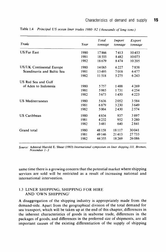
The unit of measurement of the volume of production or supply in shipping is all important. The number of tons (measured in weight) of cargo carried or of capacity offered is not satisfactory, and for two reasons: (i) tons should be weighted by the distance travelled; the number of ton-miles is therefore a superior measure, and (ii) in practically all liner trades volume rather than weight determines the constraint to the carrying capacity; therefore, the number of cubic ton-miles (measured in cubic meters) is a superior measure to the number of weight ton-miles. An example of the importance of distance is the fact that between the end of the 1940s and the middle of the 1970s the annual rate of growth in total ton-miles (in weight) by sea was as high as 12% compared with 8% in tons. The average transport distance has been rising. The rapid economic growth of Japan, the expansion of oil exports from the Persian Gulf to the distant markets of USA and Europe, and the opening of new sources of minerals in Africa, Australia and Brazil, are the main explanation of this observation. An example of the importance of measuring in cubic meters is the liner trade between USA and the Far East. During the years 1980-82 westbound weight tonnage (exports from USA) was 26% higher than eastbound tonnage (see Table 1.4). When measured in volume, the imbalance is reversed. Capacity utilization on the eastbound leg was greater than 90% during that period compared to a utilization of less than 60% on the westbound leg, when the two are measured by the volume of cargo. *
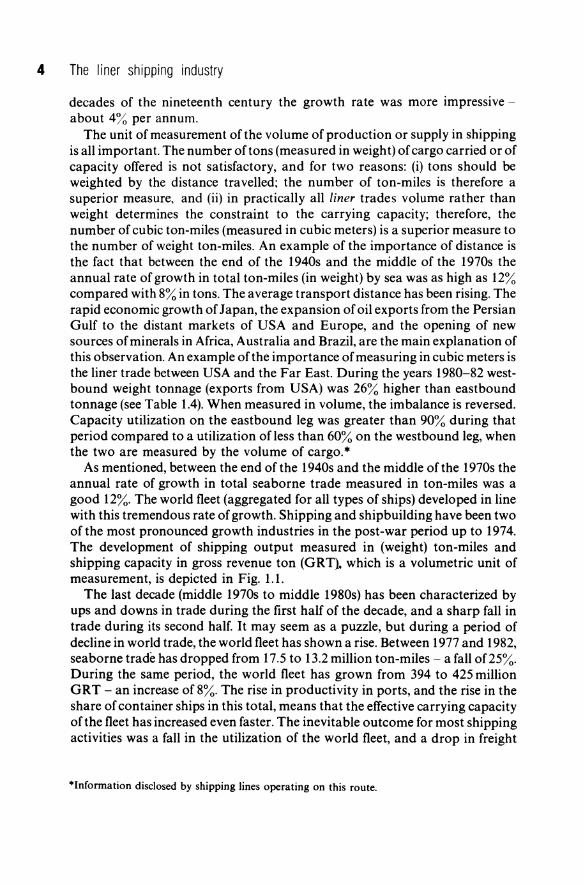
As mentioned, between the end of the 1940s and the middle of the 1970s the annual rate of growth in total seaborne trade measured in ton-miles was a good 12%. The world fleet (aggregated for all types of ships) developed in line with this tremendous rate of growth. Shipping and shipbuilding have been two of the most pronounced growth industries in the post-war period up to 1974. The development of shipping output measured in (weight) ton-miles and shipping capacity in gross revenue ton (GRT). which is a volumetric unit of measurement, is depicted in Fig. 1.1.
The last decade (middle 1970s to middle 1980s) has been characterized by ups and downs in trade during the first half of the decade, and a sharp fall in trade during its second half. It may seem as a puzzle, but during a period of decline in world trade, the world fleet has shown a rise. Between 1977 and 1982, seaborne trade has dropped from 17.5 to 13.2 million ton-miles - a fall of 25%. During the same period, the world fleet has grown from 394 to 425 million GRT - an increase of 8%. The rise in productivity in ports, and the rise in the share of container ships in this total, means that the effective carrying capacity of the fleet has increased even faster. The inevitable outcome for most shipping activities was a fall in the utilization of the world fleet, and a drop in freight
·Information disclosed by shipping lines operating on this route.
"!j
~.
; -;... >-l
::r
(l>
0-
(l>
<:
(l
> 0- '0 3 (l
>
::l ... o ...,
~
~ o §:
'" (l> ~ r:T
o ... ::l
(l>
... ... ~ 0-
(l>
~
::l
0- ~
~ o ... 0::
::>
8 ... ... o ::l
::l
~ ~
0" 19
19
19
19
19
196
196
197
197
197
197
197
I i I I I
197
197
197
1978
19
79
1980
1981
19
82
1983
o o
I I I Mill
ion
G
RT
I I N o o I I I I I
w
o o I I J I
I
.". o l I I
o 196
196
196
196
196
197
197
197
197
197
197
197
197
1978
19
7 19
80
198
1982
19
83 I
lJ1 o o o
I I Mill
iard
to
n -
mile
s
I I I o o o o
I I
I I J
- <.n o o
I I I J 1 J I I J
N o o o
6 The liner shipping industry
rates. The recession that started at the beginning of the 1980s, has plunged still deeper and is likely to stick until the end of the decade.
What explains the lack of response of supply to the fall in demand and the continuous increase in shipping capacity in spite ofthe drop in total ton-miles? We suggest two explanations, one technological and the other institutional. The last ten years were a period of rapid technological development which was triggered by the rise in fuel costs.
The most important technological innovation has been the development of fuel-saving engines. New diesel engines equipped with computers that coordinate the diesel-fuel characteristics with the timing of ignition, save up to 20 tons of fuel out of 66 tons of daily fuel consumption of a middle-size container ship - approximately 30% savings. In 1984 there were about 300 orders for Sulzer's RTA newly developed engine and 250 for the MANB& WL-M C engine.
The fuel-saving operation is not limited to the efficient engine. It has been widely recognized, for instance, that the ship's propeller, in its present form, is quite an obsolete concept. Much progress has been made in experiments with new ideas, like that of Bremer Vulkan, which decreases fuel consumptionly 10%. The new propeller arrangement consists of a conventional four-blade propeller fitted with a second nine-blade reaction propeller. This second propeller, mounted behind the conventional one and not being connected to the engine, turns independently. The inner part of the reaction propeller is curved; it acts as a turbine, the nine blades being driven by the outflow of the four-blade unit. This produces a moment of rotation, which is converted into thrust, which can be used to attain higher speed or to reduce the actual power required from the main engine, thereby reducing fuel consumption.
Hull design and hull cleaning also have had an effect on fuel saving. In 1984 Japanese yards were building twenty bulk carriers for Sanko with a bulbous open stern that reduces friction and improves flow to the propeller and thereby reduces power requirements up to 4%. The inventors of the bulbous open stern maintain that it can be applied to any type of ship. Sandblasting and selfpolishing coatings have also proved to be efficient fuel-saving techniques.
There have been other innovations, for example, the 'Racal-DeccaNavigator' which incorporates in one system practically all the existing navigational instruments, and the Swedish fuel-economizer (Sal-Fe), which keeps watch on the vessel's long-term performance, including fuel quality.
Ships in this era of rapid technological changes have a much shorter life than before. At the beginning ofthe century, ships 50 or 60 years old were still sailing the seas. The Liberty ships were still in operation 30 years after the Second World War. Today, a 15-year-old container ship is considered obsolete. The life-span of a container ship is taken today to be 12 years.
Some institutional factors acted to increase the tendency for more ship building. First, governments protecting employment interests continued to
Characteristics of demand and supply 7
subsidize shipyards. Second, international intervention - in the form of the UNCT AD formula for sharing trade (see chapter 2), have triggered a development of national fleets by the developing countries. The high level of new shipbuilding orders in 1981 and 1982 will prolong the excess capacity, and may present shipping during the rest of the 1980s with the least favourable business environment the industry has known since the Second Warld War.
1.2 THE DEVELOPMENT OF THE SHARES OF THE WORLD FLEET: DEVELOPED COUNTRIES, FLAGS OF CONVENIENCE AND DEVELOPING COUNTRIES
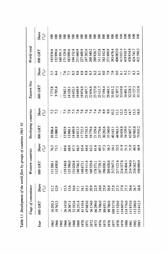
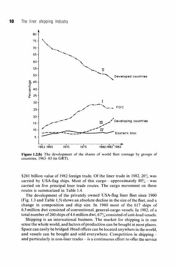
This description of the development of the world fleet concentrates on the changes in its composition by flag in the last twenty years. With the help of Table 1.1 and Fig. 1.2 we see that the fleet of the traditional maritime countries has nearly doubled during the period, while both the flags of convenience* category and the fleet of developing countries has shown a sevenfold increase. These different rates of growth mean that the shares of these groups of countries have changed substantially during the period. Most notable is the decline in the share of developed countries which has gone down by approximately 30%. Flags of convenience have increased their share from 11 % to 28% between 1963 and 1977, but show a slight decline since then. The fleet of developing countries has increased its share from 7% to 18% at an accelerating rate. The Eastern bloc has maintained a fairly constant share throughout the period of approximately 8%.
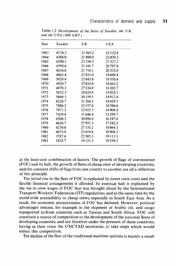
The development of two traditional maritime nations - the UK and Sweden - and that of the USA is shown in Table 1.2 and Fig. 1.3. In 1983 the size of the British fleet was less than that in 1963, and its share has declined from 15% to 5.5%. The share of the USA has dropped from 19.1 % in 1960 to 4.6% - a decline of almost four times. Similarly, the size of the fleet under the Swedish flag has declined during the period, and its share has gone down from 3% to 1%.
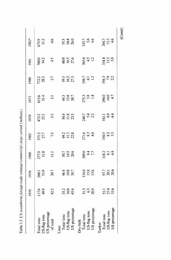
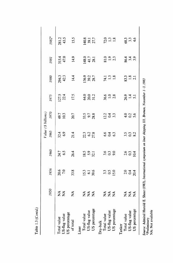
Of the developed countries the share of the USA-flag carriage of seaborne foreign trade to/from the USA has been strikingly low - below 5% - since 1975. Table 1.3 summarizes the development of this trade since 1950. Of a total of 676 million tons handled in 1982, non-liner dry-bulk shipments accounted for half this tonnage, tanker cargo represented 42%, and liner cargo constituted the remaining 8%. Thus, the 55.5 million tons of liner cargo were but a small fraction of the total trade, but they represented half of the
* A flag of convenience is characterized by the following features: (i) The country of registry allows ownership and control of vessels by non-citizens. (ii) Taxes on the income from the ships are not levied locally or are low. (iii) Manning of ships by non-nationals is freely permitted. (iv) There is little control and few regulations by the government over the shipping. Countries affording 'flags of convenience', or 'open registry flags', are Liberia, Panama, Cyprus and Somalia. Of these only Liberia and Panama have a substantial open-registry fleet.
Tab
le 1
.1
Dev
elop
men
t o
f the
wor
ld fl
eet
by g
roup
s o
f cou
ntri
es 1
963-
83
Fla
gs o
f con
veni
ence
W
este
rn c
ount
ries
D
evel
opin
g co
untr
ies
Eas
tern
blo
c W
orld
tot
al
Year
00
0 G
RT
Sh
are
000
GR
T
Shar
e 00
0 G
RT
Sh
are
000
GR
T
Shar
e 00
0 G
RT
Sh
are
(%)
(%)
(%)
(%)
(%)
1963
16
295.
3 11
.2
1112
88.1
76
.3
10 5
06.4
7.
2 77
73.8
5.
3 14
5836
.6
100
1964
19
763.
3 12
.9
1124
50.0
73
.5
1100
0.9
7.2
9785
.4
6.4
1529
99.6
10
0
1965
16
0391
.5
100
1966
26
143.
0 15
.3
1191
40.8
69
.6
1290
3.9
7.5
1294
2.1
7.6
1711
29.8
10
0
1967
28
387.
5 15
.6
1253
96.0
68
.9
13 9
88.1
7.
9 14
328.
1 7.
7 18
2099
.6
100
1968
32
182.
6 16
.6
1310
28.8
67
.5
1448
8.9
7.5
1645
2.1
8.5
1941
52.4
10
0
1969
36
251.
4 17
.1
1407
46.3
66
.5
1601
3.3
7.6
1864
9.9
8.8
2116
60.9
10
0
1970
41
119.
4 18
.1
1486
73.1
65
.4
1772
2.5
7.8
1997
4.9
8.8
2274
89.9
10
0
1971
47
683.
0 19
.3
1591
11.6
64
.4
1871
0.3
7.6
2169
7.7
8.8
2472
02.6
10
0
1972
56
174.
0 20
.9
1695
29.8
63
.2
1977
9.6
7.4
2285
6.8
8.5
2683
40.2
10
0
1973
66
299.
0 22
.9
1785
71.1
61
.6
2132
9.6
7.4
2372
7.0
8.2
2899
26.7
10
0
1974
74
706.
0 24
.0
1877
28.3
60
.3
2377
6.6
7.6
2511
1.7
8.1
3113
22.6
10
0
1975
88
655.
3 25
.9
1960
30.1
57
.3
3028
2.6
8.9
2719
4.4
8.0
3421
62.4
10
0
1976
99
786.
0 26
.8
2094
30.8
56
.3
3334
0.0
9.0
2944
3.1
7.9
3719
99.9
10
0
1977
10
9517
.0
27.8
21
2947
.1
54.1
40
163.
1 10
.2
3105
1.2
7.9
3936
78.4
10
0
1978
11
1520
.0
27.5
21
7121
.6
53.5
44
963.
3 11
.1
3239
7.2
8.0
4060
02.0
10
0
1979
11
4605
.0
27.8
21
4337
.8
51.9
50
458.
8 12
.2
3361
9.8
8.1
413
021.
4 10
0
1980
11
4776
.0
27.3
21
6404
.3
51.5
54
329.
0 12
.9
3440
1.3
8.2
4199
10.7
10
0
1981
11
1855
.0
26.6
21
4744
.0
51.0
62
007.
5 14
.7
3222
8.3
7.7
4208
34.8
10
0
1982
11
3288
.0
26.7
21
0342
.7
49.5
65
983.
8 15
.5
3512
7.2
8.3
4247
41.7
10
0
1983
11
3412
.3
26.8
19
8090
.0
46.9
75
935.
2 18
.0
3515
2.8
8.3
4225
90.3
10
0

..... a:: (!)
0 0 0 0 0 0
450
400
350
300
250
200
150
100
50
. /' ..... ..--.
/" ./ ..
./. ./
World I"ol"al
n. ."",. .. ~ ......... I.· --,.Developed countries
.. /.. "
/'
/
I _.-·-·_·-FOC ".
.// ", m /- Developing countries
./ ."
." " ." /'" lY .-' _ --""" Easl"ern bloc • ..-_fIIIII' ,<~
", . .".,. ----~ --..., ~-
1963 1965 1970 1975 19801982 1983
Figure 1.2(a) Development of the world fleet (000 GRT), by groups of countries.
10 The liner shipping industry
BO
75
70
65
60
55
50
~ 45 E ;; 40 ~ .f. 35
30
25
20
15
10
5
'. " """. ..............
.. , .. , ..
- .... ---
1963 1965 1970
'\. ".
'_" II "- ..
I
........ Developed countries ,
Foe
, ill ~/ Developing countries
"" .... "" _ ....... - IY
Eastern bloc
1975 19BO 19B2 19B3
Figure 1.2(b) The development of the shares of world fleet tonnage by groups of countries, 1963-83 (in GRT).
$281 billion value of 1982 foreign trade. Of the liner trade in 1982, 26% was carried by USA-flag ships. Most of this cargo - approximately 80% - was carried on five principal liner trade routes. The cargo movement on these routes is summarized in Table 1.4.
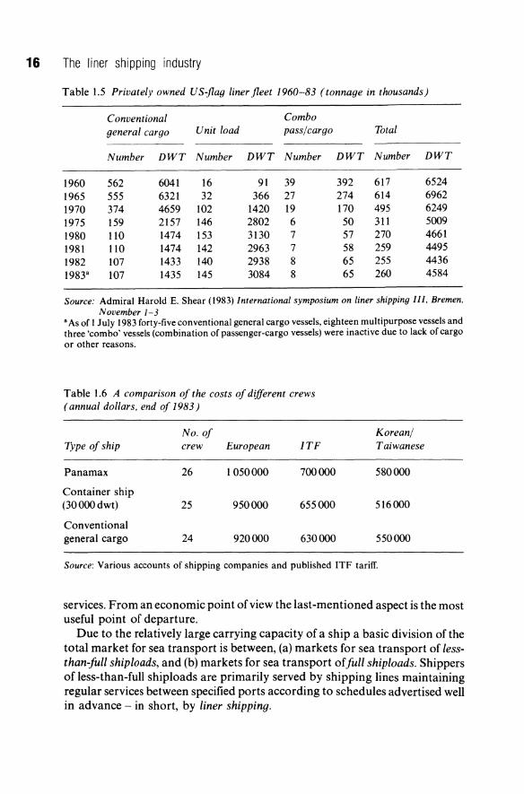
The development of the privately owned USA-flag liner fleet since 1960 (Fig. 1.3 and Table 1.5) shows an absolute decline in the size of the fleet, and a change in composition and ship size. In 1960 most of the 617 ships of 6.5 million dwt consisted of conventional, general-cargo vessels. In 1982, of a total number of260 ships of 4.6 million dwt, 67% consisted of unit-load vessels.
Shipping is an international business. The market for shipping is in one sense the whole world, and factors of production can be bought at most places. Space can easily he bridged. Head offices can be located anywhere in the world, and vessels can be bought and sold everywhere. Competition in shipping -and particularly in non-liner trades - is a continuous effort to offer the service
Characteristics of demand and supply
Table 1.2 Development oj the fleets oj Sweden, the UK and the USA (000 GRT)
Year Sweden UK USA
1963 4176.3 21565.2 23132.8 1964 4308.0 21490.0 22430.2 1965 4290.1 21530.3 21527.3 1966 4399.6 21541.7 20797.4 1967 4634.6 21716.1 20332.6 1968 4865.4 21921.0 19668.4 1969 5029.4 23843.8 19550.4 1970 4920.7 25824.8 18463.2 1971 4978.3 27334.9 16265.7 1972 5632.3 28624.9 15024.1 1973 5669.3 30159.5 14912.4 1974 6226.7 31566.3 14429.1 1975 7486.2 33157.4 14586.6 1976 7971.2 32923.3 14908.4 1977 7429.4 31646.4 15299.7 1978 6508.3 30896.6 16187.6 1979 4636.7 27951.3 17542.2 1980 4234.0 27135.2 18464.3 1981 4033.9 25419.4 18908.3 1982 3787.6 22505.3 19111.1 1983 3432.7 19121.5 19358.5
at the least-cost combination of factors. The growth of flags of convenience (FOC) and its halt, the growth of fleets of cheap crew of developing countries, and the constant shifts of flags from one country to another are all a reflection of this principle.
The initial rise in the fleet of FOC is explained by lower crew costs and the flexible financial arrangements it afforded. Its eventual halt is explained by the rise in crew wages of FOC that was brought about by the International Transport Workers' Federation (ITF) regulations, and at the same time by the world-wide accessibility to cheap crews, especially in South East Asia. As a result, the economic attractiveness of FOC has declined. However, political advantages remain, for example in the shipment of Arabic oil, and cargo transported to/from countries such as Taiwan and South Africa. FOC still constitute a source of competition to the development of the national fleets of developing countries, and are therefore under the pressure of these countries, having as their voice the UNCT AD secretariat, to take steps which would reduce this competition.
The decline of the fleet of the traditional maritime nations is mainly a result
11
12 The liner shipping industry
15
14
13 \
12 \ \
11 \ \ \ 10 \
GI \ 0'1 9 0 \ ..... c: \ cu 8 u \ ... cu \ 0- 7
\ 6 \
\ , 5 .... , -' 4 "- ,,- USA --" 2
3 ...... _ ....... _. -._.-._ ........ "
''-'-'_Sweden
1963 1965 1970 1975 19801982 1983
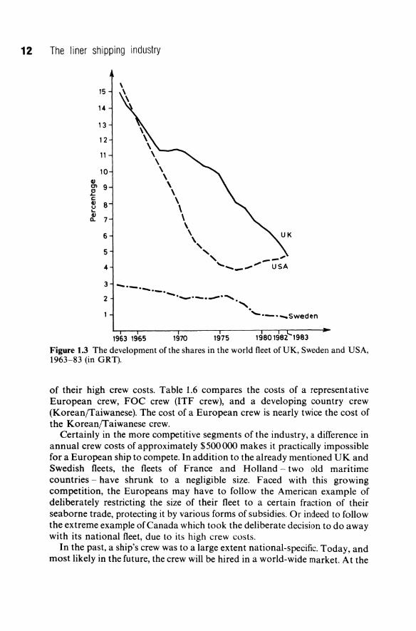
Figure 1.3 The development of the shares in the world fleet of UK, Sweden and USA, 1963-83 (in GRT).
of their high crew costs. Table 1.6 compares the costs of a representative European crew, FOC crew (ITF crew), and a developing country crew (Korean/Taiwanese). The cost of a European crew is nearly twice the cost of the Korean/Taiwanese crew.
Certainly in the more competitive segments of the industry, a difference in annual crew costs of approximately $500000 makes it practically impossible for a European ship to compete. In addition to the already mentioned UK and Swedish fleets, the fleets of France and Holland - two old maritime countries - have shrunk to a negligible size. Faced with this growing competition, the Europeans may have to follow the American example of deliberately restricting the size of their fleet to a certain fraction of their seaborne trade, protecting it by various forms of subsidies. Or indeed to follow the extreme example of Canada which took the deliberate decision to do away with its national fleet, due to its high crew costs.
In the past, a ship's crew was to a large extent national-specific. Today, and most likely in the future, the crew will be hired in a world-wide market. At the
Tab
le 1
.3
US
ocea
nbor
ne[o
reig
n tr
ade
tonn
age/
com
mer
cial
car
go c
arri
ed (
mil
lion
s)
1950
19
56
1960
19
65
1970
19
75
1980
19
81
1982
"
Tot
al t
ons
117.
6 26
0.1
277.
9 37
1.3
473.
2 61
5.6
772.
2 76
0.0
675.
9 U
S-f
lag
tons
49
.9
53.9
31
.0
27.7
25
.2
31.4
28
.2
34.2
31
.2
US
per
cent
age
of
tota
l 42
.5
20.7
11
.1
7.5
5.3
5.1
3.7
4.5
4.6
Lin
er
Tot
al t
ons
35.2
46
.4
50.7
49
.2
50.4
44
.3
59.3
60
.0
55.5
U
S-f
lag
tons
16
.0
18.0
14
.5
11.2
11
.8
13.6
16
.2
16.5
14
.4
US
per
cent
age
45.6
38
.7
28.6
22
.8
23.5
30
.7
27.3
27
.6
26.0
Dry
-bul
k T
otal
ton
s 31
.3
116.
0 10
9.0
171.
6 24
0.7
275.
3 35
6.7
365.
6 33
5.7
US
-fla
g to
ns
6.5
15.8
8.
4 8.
2 5.
4 3.
8 4.
1 4.
5 3.
6 U
S p
erce
ntag
e 20
.9
13.6
7.
7 4.
8 2.
2 1.
4 1.
2 1.
2 4.
6
Tan
ker
T
otal
ton
s 51
.1
97.7
11
8.2
150.
5 18
2.1
296.
0 35
6.3
334.
4 28
4.7
US
-fla
g to
ns
27.4
20
.1
8.1
8.2
8.0
14.0
7.
9 13
.2
13.2
US
per
cent
age
53.6
20
.6
6.9
5.5
4.4
4.7
2.2
3.9
4.6 (C
ontd
.)
Tab
le 1
.3 (
Con
td.)
Val
ue (
$ b
illi
ons)
1950
19
56
1960
19
65
1970
19
75
1980
19
81
1982
"
Tot
al v
alue
N
A
20.6
24
.7
32.4
49
.7
127.
5 29
4.3
315.
4 28
1.2
US-
flag
valu
e N
A
7.0
6.5
6.9
10.3
22
.4
42.3
47
.0
43.5
U
S pe
rcen
tage
of
tota
l N
A
33.8
26
.4
21.4
20
.7
17.5
14
.4
14.9
15
.5
Lin
er
Tot
al v
alue
N
A
15.3
18
.5
22.3
33
.5
64.0
13
6.9
148.
0 14
0.8
US-
flag
valu
e N
A
6.1
5.9
6.2
9.7
20.0
39
.2
41.7
39
.1
US
perc
enta
ge
NA
39
.6
32.1
27
.8
28.8
31
.2
28.7
28
.1
27.7
Dry
-bul
k T
otal
val
ue
NA
3.
3 3.
6 6.
6 12
.2
36.6
74
.1
81.0
72
.0
US-
flag
valu
e N
A
0.5
0.3
0.4
0.4
1.0
1.3
1.9
1.3
US
perc
enta
ge
NA
15
.0
9.0
6.3
3.3
2.8
1.8
2.3
1.8
Tan
ker
Tot
al v
alue
N
A
2.0
2.6
3.5
4.0
26.9
83
.3
86.4
68
.3
US-
flag
valu
e N
A
0.4
0.3
0.3
0.2
1.4
1.8
3.4
3.3
US
perc
enta
ge
NA
20
.4
10.4
8.
2 5.
6 5.
1 2.
1 3.
9 4.
6
Sour
ce:
Adm
iral
Har
old
E. S
hear
(198
3), I
nter
natio
nal
sym
posi
um o
n lin
er s
hipp
ing
III.
Bre
men
, N
ovem
ber
1-3.
198
3 • P
relim
inar
y N
A:
Not
ava
ilabl
e
Characteristics of demand and supply
Table 1.4 Principal US ocean liner trades 1980-82 (thousands of long tons)
Total Import Export Trade Year tonnage tonnage tonnage
US/Far East 1980 17866 7413 10453 1981 18555 8482 10073 1982 18679 8474 10205
US/UK Continental Europe 1980 14065 6227 7838 Scandinavia and Baltic Sea 1981 13495 7018 6477
1982 11 518 5275 6243
US Red Sea and Gulf of Aden to Indonesia 1980 5757 1488 4269
1981 5985 1731 4254 1982 5673 1450 4223
US Mediterranean 1980 5636 2052 3584 1981 6879 3230 3649 1982 5004 2430 2574
US Caribbean 1980 4834 937 3897 1981 4232 952 3280 1982 3481 640 2841
Grand total 1980 48158 18117 30041 1981 49146 21413 27733 1982 44355 18269 26086
Source: Admiral Harold E. Shear (1983) International symposium on liner shipping III, Bremen, November 1-3
same time there is a growing concern that the potential market where shipping services are sold will be restricted as a result of increasing national and international intervention.
1.3 LINER SHIPPING, SHIPPING FOR HIRE AND 'OWN SHIPPING'
A disaggregation of the shipping industry is appropriately made from the demand-side. Apart from the geographical division of the total demand for sea transport, which will be taken up at the end of this chapter, differences in the inherent characteristics of goods in seaborne trade, differences in the packages of goods, and differences in the preferred size of shipments, are all important causes of the existing differentiation of the supply of shipping
15
16 The liner shipping industry
Table 1.5 Privately owned US-flag liner fleet 1960-83 (tonnage in thousands)
Conventional Combo
general cargo Unit load pass/cargo Total
Number DWT Number DWT Number DWT Number DWT
1960 562 6041 16 91 39 392 617 6524 1965 555 6321 32 366 27 274 614 6962 1970 374 4659 102 1420 19 170 495 6249 1975 159 2157 146 2802 6 50 311 5009 1980 110 1474 153 3130 7 57 270 4661 1981 110 1474 142 2963 7 58 259 4495 1982 107 1433 140 2938 8 65 255 4436 1983" 107 1435 145 3084 8 65 260 4584
Source: Admiral Harold E. Shear (1983) International symposium on liner shipping III, Bremen, November /-3
"As of I July 1983 forty-five conventional general cargo vessels, eighteen multipurpose vessels and three 'combo' vessels (combination of passenger-cargo vessels) were inactive due to lack of cargo or other reasons.
Table 1.6 A comparison of the costs of different crews (annual dol/ars, end of 1983)
No. of Korean/ Type of ship crew European ITF Taiwanese
Panamax 26 1050000 700000 580000
Container ship (30000dwt) 25 950000 655000 516000
Conventional general cargo 24 920000 630000 550000
Source: Various accounts of shipping companies and published ITF tariff.
services. From an economic point of view the last-mentioned aspect is the most useful point of departure.
Due to the relatively large carrying capacity of a ship a basic division of the total market for sea transport is between, (a) markets for sea transport of lessthan-full shiploads, and (b) markets for sea transport offull shiploads. Shippers of less-than-full shiploads are primarily served by shipping lines maintaining regular services between specified ports according to schedules advertised well in advance - in short, by liner shipping.

Fin
al
m a
nufac~ured
go
od
s, fru
i~,
vege~ables a
nd
fr
oze
n m
ea
l"
Inte
rme
dia
l"e
g
oo
ds
Pro
cess
ed
m
al"
eri
al
Ra
w m
ate
ria
l
Typ
e o
f g
oo
ds
Ca
rl"o
ns
Bo
xe
s
Cra
l"e
s
Un
pa
cke
d b
ig
art
icle
s (
e.g
ca
rs)
Ba
gs
Dru
ms
Ba
les,
ro
lls
e~c.
Typ
e o
f p
ack
ag
e
DE
MA
ND
Sm
all
ship
me
nl"
s a
t sh
orl
"er
or
I •
I lo
ng
er
inte
rva
ls
Me
diu
m-s
ize
sh
ipm
en
l"s
Fu
ll sh
iplo
ad
s _I
o
nce
or
tWic
e
a ye
ar
Lin
er
ship
pin
g
Sh
ipp
ing
fo
r h
ire
Sh
ipp
ing
un
de
r yo
ur
ow
n
Fu
ll sh
iplo
ad
s H
sl
"eam
('o
wn
m
an
y h
me
s
ship
pin
g ')
a
ye
ar
Siz
e a
nd
an
nu
al
nu
mb
er o
f shipmen~
Typ
e o
f sh
ipp
ing
se
rvic
e
SU
PP
LY
Figu
re 1
.4 S
hipp
ing
dem
and
and
supp
ly a
spec
ts.
Bre
ak-b
ulk
ca
rgo
sh
ips
('co
nve
nh
on
al
line
rs>
)
Bre
ak-b
ulk
ca
rgo
sh
ip
wit
h o
ne
or
mo
re ref
rige
ra~e
d h
old
s
Sp
eci
aliz
ed
'u
nit
lo
ad
' ca
rrie
rs
All-
pu
rpo
se
~ramp s
hip
s
Sp
eci
aliz
ed
d
ry-b
ulk
ca
rrie
rs a
nd
o
il I"
an
kers
Typ
e o
f sh
ip
18 The liner shipping industry
Shippers of full shiploads rely on the ship charter market. They can either enter a long-term charter agreement which may have a duration of6 months to 20 years and more, or they may enter a single-voyage charter agreement, and make use of the spot charter market. Full shiploads make possible 'shipping for hire' transactions - either short or long term.
The development of telecommunication has greatly facilitated the continuous matching of shipping capacity and potential shiploads, which is a prerequisite for the working of a voyage charter market. However, the Baltic Exchange in London, the most important auction market for tramp-ship charters, originated in the 18th century.
We think it is instructive to speak about 'own shipping' (an abbreviation of our own making) as the third main type of shipping services (see Fig. 1.4). Historically 'own shipping' has the oldest origin at least so far as deep-sea shipping is concerned. As the term suggests, merchant shipping used to be conducted by big merchants and trading firms like the East India Company, which had more or less monopolized each particular trade. They owned the ships which carried their goods, and there was not much room for special shipping companies. As international trade grew, however, new demands for shipping arose.
The general technological progress made possible specialization in shipping. The two catalysts for the emergence of liner shipping and voyage charter shipping, were respectively the introduction of steamships during the second half of the nineteenth century which made possible regular shipping services according to schedule, and the development of telecommunication. With these developments 'own shipping' tonnage was offered for the general use by the big trading companies, and shipping lines were thus formed. Today 'own shipping' is confined to specialized shipping activity, especially in the -bulk-shipping market. About one-half of the world tanker fleet is owned or long-time chartered by the oil companies. In the dry-bulk market about 30% of the tonnage is owned by industrial companies.
1.3.1 Shipping activities and ship types
We distinguish three main types of shipping activities: 'liner services', 'shipping for hire', and 'own shipping'. In the past all three activities were served by ships of an 'all-purpose' type. Shipping-for-hire services had mostly been carried out by the so-called 'tramps'. The traditional tramp used to be an all-purpose ship. The idea behind such a ship was to maximize the chances of getting a cargo in any port of the world. The tramp would go to a port wherever and whenever sufficient cargo was available to fill the ship. The ships employed in liner shipping were, like the tramps, exclusively all-purpose ships. The important difference was that liners were designed to carry miscellaneous packaged cargo. That meant in the first place that the liners were equipped with two or

Characteristics of demand and supply 19
more decks. They were also usually faster than the tramps, which is a reflection of the higher average value of time of packaged cargo.
The similarity of the ship types meant that they were all, at least potentially, in competition with each other. Although the main space in the lower holds of a typical all-purpose tramp was intended for loose cargo or big lots of robust packaged cargo, it could also stow small packaged cargo on the single shelter deck. This also meant that conversions of tramps into liners and liners into tramps were not too involved. It was not unusual that an original liner ended its days as a tramp. Or, that a shipping line would occasionally charter a suitable tramp ship for one or more sailings.
The potential savings of specialization and tailor-made ships, have embraced all types of shipping activities. The traditional all-purpose tramp has practically disappeared from the seas. Shipping-for-hire services are nowadays carried out by specialized bulk carriers designed to take one or two types of cargo (e.g. ore and oil, carried by Ore-Bulk-Oil (OBO) ships). Similarly own shipping is nowadays performed by specialized ships. The main point of owning ships for a large goods producer/exporter is that a high degree of cost-reducing specialization of the ships' design can be ventured. The tendency to specialization has also influenced the design of liners. The disadvantages of handling very heterogeneous articles have been mitigated by introducing standard 'unit loads'. Special ships go with each particular type of unit load. Containers and container ships are the dominant and most well-known examples of this development. In 1985 approximately 60% of the liner cargo was carried by the general category of container ships, while the remaining 40% by the non-container category, called 'conventional liners'.
An outcome of the tendency to specialization is that competition between the different types of shipping activities has greatly declined. In particular, the traditional competition between the liner and the all-purpose tramp belongs to the past.
In the future, some competition between the liners and tramp will remain, and will take two forms. First, there are bulk ships that are designed to take both bulk and general cargo or containers. These are few in number and do not constitute a severe threat to the liner trade. One example is the Belgian ABC line, which has been operating six specially designed vessels which can carry both bulk and containers on the Australia-Europe and USA trade routes. The other form of competition is simply that with the general increase in the volume of international trade, the borderline between general cargo and bulk will gradually shift. Some commodities that were potential liner cargo (such as sugar and rice) will become minor bulk, moving in quantities that are sufficient to fill a ship.
Yet, the main source of competition in the liner shipping industry is the liners themselves - either by the independents operating outside the conferences, or by member lines operating within the conferences.
20 The liner shipping industry
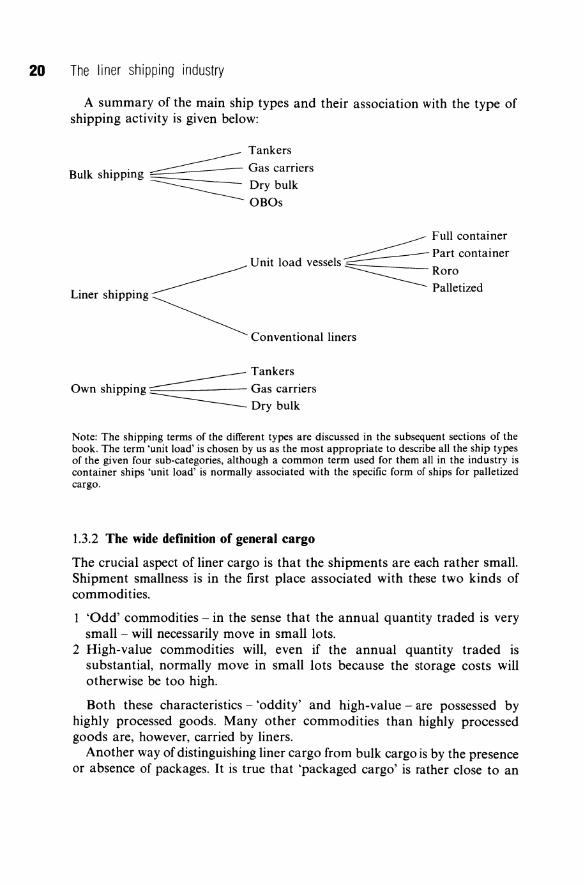
A summary of the main ship types and their association with the type of shipping activity is given below:
Tankers
Bulk shipping ~ Gas carriers -----======- Dry bulk OBOs
__________ Full container
~Part container _________ Unit load vessels ~ Roro
L· h" ---------- Palletized mer s Ippmg
~ Conventionailine"
____ Tankers
Own shipping Gas carriers
----Dry bulk
Note: The shipping terms of the different types are discussed in the subsequent sections of the book. The term 'unit load' is chosen by us as the most appropriate to describe all the ship types of the given four sub-categories, although a common term used for them all in the industry is container ships 'unit load' is normally associated with the specific form of ships for palletized cargo.
1.3.2 The wide definition of general cargo
The crucial aspect of liner cargo is that the shipments are each rather small. Shipment smallness is in the first place associated with these two kinds of commodities.
'Odd' commodities - in the sense that the annual quantity traded is very small - will necessarily move in small lots.
2 High-value commodities will, even if the annual quantity traded is substantial, normally move in small lots because the storage costs will otherwise be too high.
Both these characteristics - 'oddity' and high-value - are possessed by highly processed goods. Many other commodities than highly processed goods are, however, carried by liners.
Another way of distinguishing liner cargo from bulk cargo is by the presence or absence of packages. It is true that 'packaged cargo' is rather close to an
Characteristics of demand and supply 21
exhaustive definition of liner cargo. Exceptions certainly exist. On one hand, articles like cars or logs are often carried by liners in an unpacked shape. On the other hand, large shipments of bagged cargo, for example, can go by bulk shipping.
The real snag of this criterion of distinction is that 'packaged or loose' is not an inherent characteristic of commodities. It is not a characteristic which leads to smallness of shipments, but the causal relationship is the opposite. No matter whether the shipper wants it or not, the goods of a small shipment have normally to be packed in order to 'mix' with other shipments of packaged cargo. This has to be done for stowage reasons, but, of course, also for their own protection, or to avoid causing damage to other goods.
The so-called 'major bulk commodities' - oil, iron ore, coal, bauxite, phosphate rock, grain, and perhaps a few others - are nowadays traded in such large quantities that they come in shiploads in practically all trades. Under this condition transport in loose form will, besides the savings of package costs, make possible the most economic methods of port handling, and the most economic modes of shipping. It is not that these bulk commodities are inherently unsuitable for packaging. For instance, oil in drums used to be a common liner cargo, as recently as in the 1920s.
The conclusion is that liner cargo cannot be defined operationally as a goods category which is predestined to liner shipping. It is useful to divide the total seaborne trade into 'the major bulk commodities', on one hand, and the rest, which can be called general cargo', on the other. Liner shipping has practically nothing to do with the former category. The latter category, is however, by no means reserved for liner shipping. Specialized bulk carriers, that either operate in the spot market, or in the time-charter market, make inroads into liner shipping.
The most important sub-class of general cargo for liner services in terms of freight revenue is final consumer and producer goods - manufactures, textiles, food products etc., tools and machinery. Lawrence (1972, p. 137) estimates that these shipments account for only 10-15% of the general cargo weight, but constitute more than half of all general cargo by value.
Second in importance is what can be loosely described as intermediate goods. Chemicals, steel products and various assembly parts belong to this category. The growth of multinational firms, and the international division of production processes has given a stimulus to trade in intermediate goods.
The third general cargo category is primary products and such processed goods as boards, wood pulp and paper, cement, copper and other metals, scrap iron, etc. These commodities are shared with tramps and specialized bulk carriers. The share of liner shipping in this trade is quite sensitive to relative freight rates.
Finally, the wide definition of general cargo nowadays includes the most important category of unitized cargo - containers, trailers, pallets, etc.
22 The liner shipping industry
1.4 THE RELATIVE SIZE OF THE LINER SHIPPING INDUSTRY
It is remarkable that there exists no published records of the total turnover, value added, or some other measure of the size in economic terms of the liner shipping industry. The main reason for this is probably that liner shipping companies, unless forced to do so, do not bother to report this kind of data. However, estimates of total liner shipping turnover have from time to time been produced on an ad hoc basis. There seems to be a reasonable consensus about the relative importance of liner shipping: total resource costs of liner shipping are about the same as the resource costs of all other branches of shipping put together. For example, in the Rochdale report it was estimated that 'the gross revenue ofthe liner trades amounts to perhaps about one half of the total revenue of the shipping industry' (HMSO, 1970).
In terms of cargo tons, ton-miles, or fleet tonnage the relative size of the liner shipping sector appears much smaller. But neither can this be shown with accurate figures, due to lack of data. * Total ton-miles of general cargo (which is perhaps twice that of liner cargo) and total tonnage of ships for general cargo, can be given and related to the totals of all shipping. From the previously mentioned sources of shipping and seaborne trade statistics, we have extracted these round figures:
Total ton-miles of general cargo: Total dwt of ships for general cargo: Total GRT of ships for general cargo: Total freight revenue of general cargo:
One-fifth of total ton-miles of all seaborne trade One-fifth of total dwt of world fleet One-quarter of total GRT of world fleet Two-thirds of total freight revenue
1.5 RECENT DEVELOPMENT IN GENERAL CARGO SHIPPING
The fact that barely 10% of total seaborne ton-miles is produced by liners while about 50% of total freight revenue is earned in the liner shipping sector means that the average liner freight rate per ton-mile is almost ten times the average freight rate per ton-mile of all other shipping. Why is this so? This question will be fully answered in Part II, where a thorough shipping engineering economy analysis is made. A full answer requires a model which takes into account all important interrelationships between ship design variables and shipping costs.
Part of the answer is, however, very straightforward, and can be given
* An attempt to account for the liner trade between sixty pairs of countries was made by the American consulting company WAF A jointly with Mennelitics. They publish a 5-year forecast of the main commodities moving on these trades, which is updated every 6 months.

Characteristics of demand and supply 23
already at this stage. The stevedoring charges for handling heterogeneous packaged cargo are in general at least ten times higher than the stevedoring charges for handling homogeneous bulk cargo. In view of the fact that total stevedoring charges make up a good half of the total freight cost of break-bulk cargo in, for example, the North Atlantic trades and the North Pacific trades, * the relatively high direct handling (loading and unloading) costs can be said to provide half the explanation of the wide difference between liner freight rates and other shipping freight rates.
For break-bulk cargo it is generally true that the 'journey' from quay to hold and back of a shipment is more expensive than the journey across an ocean. If, in addition, the cost of ship's lay time is included, as it should be, the cost of the loading and unloading, will typically constitute two-thirds or even more of the total freight cost. In view of this rather lopsided cost structure it is not surprising that something radical had to be done about the break-bulk handling costs. The general answer to the soaring costs of stevedoring was unitization of cargo.
1.5.1 Unitization of break-bulk cargo
Break-bulk cargo handling is very labour-intensive. To minimize the lay time a big conventional liner can employ as many as ten gangs of stevedoring labour at a time, which can mean that some one hundred men are engaged in cargo handling simultaneously. (The gang size varies fairly widely from port to port.) The productivity per man-hour is very variable depending on a number of factors: the handling equipment, the type of article being handled, etc. In the port of Stockholm the round figure of 1 ton per man-hour was used as a standard in the 1950s and 1960s. Much higher figures were not reported anywhere in the ports of the world during the late 1960s and the beginning of the 1970s. Table 1.7 indicates that the productivity per gang-hour was typically less than 25 tons, and was on average in a range which corresponds to a figure somewhat above 1 ton per man-hour.
Unitization made an increase in break-bulk handling productivity possible. In 1985 the average productivity in ports of developed countries varied between 200 and 300 tons per gang shift. Given a size of a gang of ten stevedores and 8-hour shifts, 250 tons per gang-shift implies a productivity of 3 tons per man-hour: a three-fold increase over handling productivity in the 1960s.
The level of wages of longshoremen in American ports was such that the stevedoring charges for loading or unloading break-bulk cargo were in the range of $10-20 per ton at the beginning of the 1970s. The stevedoring charges
*In liner trad~sDetween deVeloping countries the proportion of total stevedoring charges in the total freight costs is much less - typically in the range of 20-30% - due to the much lower docklabour wage rate. If chronically congested ports are included in the service, the proportion of stevedoring charges is still less because the lay time cost of ships becomes very dominating.

24 The liner shipping industry
Table 1.7 Break-bulk loading and unloading capacity
Port
Antwerp and Rotterdam Bremen and Hamburg Gothenburg New York Chicago Long Beach and San Francisco Karachi Valparaiso La Valletta
Tons per gang-hour
18-25 14-22 12-20 12-18 12-20 10-15 6-22
10-18 12-15
Sources: A Battelle report pertaining to 1970 and the UNCTAD report Berth Throughput (United Nations, New York, 1973) pertaining to 1971 and 1972.
of West Europe ports were also very high, although not as high as their American counterparts. The European level of break-bulk handling costs was about half the American level.
The container made its first appearance in the 1950s, and in the latter half of the 1960s the breakthrough occurred. One used to speak about the container revolution. This is an adequate expression, which, however, should not obscure the fact that a development had been under way for some time, and can be described as a transition stage between manual break-bulk cargo handling and the container system.
One important innovation which anticipated containerization was the putting together of small-size packages to large units by pre-slinging and palletization for better utilization of crane capacity. This required equipment for lifting and carrying those units which no longer could be handled manually in ship holds and on the quay apron. The forklift truck was the most important answer to this demand.
The increase in package unit size was not without its problems. Given the conventional gear for cargo handling, the bigger units increased the risk of damage and the danger of the work. Furthermore, at least in the past, as cargo had to be lying in the open for rather long periods without protection, unpredictability of rain became an awkward problem (in the temperate zones).
The container was the logical continuation of the trend towards bigger units; it was an answer to several demands. From the handling-of-cargo point of view, by standardization of container dimensions* expensive tailor-made
·Until recently standard container dimensions were 20 x 8 x 8 feet, and 40 x 8 x 8 feet for a large one. Today a standard container has more height and is of dimensions of 20 x 8 x 8.5 feet, and 40 x 8 x 8.5 or 40 x 8 x 9.5 feet respectively. Some shipping lines are using non
standardized containers. Sea-Land still has boxes of dimensions 35 x 8 x 8 feet in use, but these are gradually being removed from operation, and American President Line (APL) are currently using 45 x 8 x 9.5 feet containers, which are not officially approved by the International Container Organization (lCO).
Characteristics of demand and supply 25
container cranes of very-high capacity could achieve sufficiently high degree of capacity utilization to be profitable. The weight per crane was raised to meet the container weight. Cranes of capacity between 30 and 45 tons were designed (container cranes of capacity of less than 30 tons are not in use, and today all new designs lift no less than 35 tons). Thanks to this and by eliminating the need for stowing the cargo in the ship's hold, the continuous work of the crane was not impeded by that notorious bottleneck.
At a container berth, where, as is usual, two container cranes are used simultaneously, fifty to sixty containers an hour can be loaded and/or unloaded, and, which is most significant, the operation does not require more than about ten men, induding the crane-operators. The productivity per manhour in this case is approximately 70 tons. Thanks to the containerization the potential man-hour productivity has risen (conservatively calculated) fifty times!
The new generation of container ships - the very large container carrier (VLCC) - of 3000 to 4400 TEUs (twenty foot equivalent units) may require more than the standard two cranes per berth, and are often supplemented by cranes of other berths. At Port Newark for example, 900-foot container ships are worked by four and sometimes by six container cranes. It should be recalled that while working, container cranes must normally have a space of a hold width between them, due to the dense container traffic on the quay.
However, bearing in mind that the lay time of ships has also been drastically reduced by cargo unitization - in the aforementioned illustrative example the handling performance per ship-hour is about 100 tons in the break-bulk case and about 700 tons in the container case - this question presents itself; Why have not all liner services already been containerized? There are three main reasons why break-bulk cargo handling still prevails in most trades.
All cargo cannot, or is not very suitable to put in a container box. 2 The tremendous labour-saving potential is somewhat of an optical illusion.
The stowage and unstowage of break-bulk cargo in the ship's hold is eliminated, but reappears to some extent in the stuffing and stripping of containers, which are second packages, so to speak.
3 The containers themselves, the container cranes, and the container ships are relatively expensive equipment.
Ofthe three the unsuitability of cargo is the most important one. In addition to the fact that some cargo is not fit to be stowed in a container, there are types of cargo that cannot be mixed within a container (raisins and coffee is an example).
Where the containerization has been carried out, a reduction in freight rates has not occurred; the cost of the capital which has been substituted for labour is very substantial. The hope is that the containerization will halt the trend of soaring freight rates, and not that it will really turn this trend downwards.
For containerization to be really labour-saving it is required that the

26 The liner shipping industry
containers are stuffed already at the premises of the shippers, and are not stripped until the containers have reached their final destinations. In these circumstances the containerization does not only save labour for loading and unloading of ships, but also eliminates the need for expensive break-bulk cargo handling at the landside of the ports, and at inland re-Ioading depots.
In developing countries the potential for door-to-door container transports has so far not seemed very great, depending among other things on the underdeveloped inland transport infrastructure; the stevedoring costs have not yet reached the critical level, where a switch from labour-intensive breakbulk cargo handling to the very capital-intensive container system is justified unless significant inland transport and handling cost savings can be achieved in addition.
A reservation to this observation is that the development of container trade does not depend only on the cost savings achieved at one end of the route. In the trade between developing and developed countries, a developing country may start container services to meet demands set by the developed country, although this development would not be justified by the cost savings of the developing country. Dar es Salaam in Tanzania and Mombasa in Kenya are examples of ports with container-service developments which aim at integrating the trade of these countries with that of the developed nations. The most captive non-containerized trade will consequently be trade between the developing countries.
Container lift-on/lift-off is the most common handling technique. Containers can also be rolled on and off, if the ship is equipped with stern-, bow- or side-ports. In that case the bogies have to be left attached to the containers in order to achieve really speedy handling, which means that the space utilization of the ship's hold cannot be as high as when the containers are stacked on each other. Two great advantages of the roll-on/roll-offtechnique are, on the other hand, (i) that the expensive container cranes are not required, and (ii) that great flexibility as to the combination of different units - containers, trailers, trucks, cars etc. - is obtained. The roll-on/roll-off technique is a development of traditional ferry services. It is predominant on short sea routes, but in the last few years roll-on/roll-off ships have spread into deep-sea trades, particularly into trades including large shipment of motor cars.
On the dense routes of the international trade, fully cellular container ships can be employed. On thin routes, the volume of cargo and the lack of port facilities may encourage the use of mix-ships. Where ports do not have liftonjIift-off container cranes, roll-on/roll-off (RoRo) ships are often being used. There are two methods of handling cargo in a RoRo ship, both requiring little port investment. According to one, any cargo - containerized or otherwise -is put on a chassis, which is connected to a tractor, which carries the load out ofthe ship and the port. Alternatively, the cargo may be put on a 'slave chassis' which is much lower and will be used only in the port area. By the other
Characteristics of demand and supply 27
method - the 'Stow-Ro' technique -large forklifts take the containers up and down the ramp and stow them in/out of the holds ofthe RoRo ship. Such ships are currently in widespread use in the thin trades, and are also used in some dense routes, e.g. the North Atlantic route.
A third unit-load system is represented by the barge-carrying vessels, which have appeared recently. As distinguished from the traditional tug towing a number or barges, the barges (lighters) are carried aboard the mother ship. The so-called lighter aboard (LASH) ships, to which a great deal of attention has been paid, can carry some seventy barges each of 850 tons holding capacity. LASH ships were built during the 1970s. There are fewabout thirty - ships of this kind operating in the mid-1980s.
There is a newer version of the LASH, which is called SEABEE, where the barges are designed according to modular dimensions of containers. LASH ships can also carry containers but are not specifically designed to do so, with the result that some idle space will remain. SEABEEs and LASHs have been operating in a number of different trades and particularly on routes between developing and developed countries. Prudential line and Lykes Brothers line, for example, operate these types of ships in the East African trade. SEABEEs and LASHs are big and expensive vessels. The penetration of container ships to many trades including those of developing countries, has lowered their attractiveness. In the mid-1980s there is no new construction of LASH and SEABEE ships.
1.5.2 Composition of the fleet of general cargo ships, and current tendencies
A decade ago, a very topical question in the shipping world was, how quick, and how far the penetration of containerization will be in liner shipping? Will something be left for conventional liners, or will this ship type be as completely replaced by unit-load carriers in the next decade, as horses were by tractors two or three decades ago? Two developments are relevant to consider: the development of the total general cargo sector, and the development of the modal split in this sector.
The most expansive part of seaborne trade in the post-war period has been the sector represented by the major bulk commodities - especially oil, coal, iron ore and grain. (So far as the oil trade is concerned the expansion came to an abrupt halt in 1975.) The general-cargo sector has been growing steadily but not at quite the same pace. In the 1970s the annual rate of growth has been a good 5%.
The total tonnage of ships for general cargo has been growing much slower in the 1970s than the general-cargo trade in ton-miles. The average rate of growth of this tonnage was only 2%. The explanation for the disparity of the trade and tonnage growth rates is two-fold.
28 The liner shipping industry
The productivity in terms of ton-miles performed per ton of deadweight has been increasing.
2 Specialized bulk carriers have made inroads into the general cargo trade.
The source of the productivity increase is easily pinpointed. During the 1970s the share of unit-load carriers of the total fleet of ships for general cargo has been steadily growing. Under otherwise equal conditions the carrying capacity in ton-miles of a container ship, or a RoRo ship is about three times greater than the carrying capacity of a conventional liner of the same tonnage. (This is probably a conservative estimate. Koike (1983), ofNYK lines, argued that 'the transport efficiency of container ships is believed to be at a level six (6) times that of conventional vessels'.) This is explained by higher speed at sea, and, above all, considerably shorter turn-around times in port of unit-load carriers.
It should, however, be remembered that the price of a container ship (including the containers) per dwt is not far from three times that of a conventional liner. The fact that the total deadweight of ships for general cargo has been slow-growing does not mean that investments in new ships have been slow.
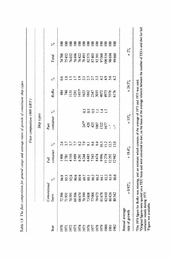
Table 1.8 below gives the composition of the general cargo fleet and the average annual rate of growth of its constituent ship types between 1970 and 1982. By the end of the period all unit-load ships measured in GRTconstituted approximately one-quarter of the total GRT of conventional liners. Bearing in mind that the productivity per GRT of unit-load ship is approximately three times greater, the liner fleet composition in terms of carrying capacity is approximately 40% unit-load ships and 60% conventional liners. Quite another matter is how the total liner cargo is divided between conventional liners and unit load carriers. The old ships do not disappear automatically as they lose business. However, Koike (1983) estimated that out of a total liner cargo trade of 1369.3 billion ton-miles, 561.3 billion ton-miles was container trade, approximately 41 % of the world liner cargo.
Lawrence (1972; p. 141) estimated that the proportion ofliner cargo carried by container ship would rise from 12% in 1970 to 35-40% by 1975 and 50-60% by 1980. This estimate seems belatedly to have come true, if the carryings of all unit-load ships are taken into account.
By the middle of 1980s it appears that the question raised a decade ago has been answered. Containerization has become the dominant form of liner shipping. By 1985 unpublished accounts of shipping lines estimate the container share in the total trade - full and part load - to be around 60%. In conjunction with the tendency to integrate land and sea transport, it can be predicted that all containerizable cargo will eventually 'go containers', with the trade between developing countries being the last to join. As to shipbuilding the rate of growth of container ship and RoRo ship investments is
Tab
le 1
.8
Th
e fl
eet
com
posi
tion
for
gen
eral
car
go a
nd a
vera
ge r
ates
of g
row
th o
f con
stit
uent
shi
p ty
pes
,Fle
et c
ompo
siti
on (
00
0 G
RT
)
Ship
typ
es
Con
vent
iona
l F
ull
Par
t Ye
ar
line
rs
%
cont
aine
r %
co
ntai
ner
%
Ro
Ro
%
T
ota
l %
1970
72
396
96.8
19
08
2.6
484
0.6
7478
8 10
0 19
71
7193
1 95
.3
2781
3.
7 74
0 1.
0 75
452
100
1972
70
591
92.8
43
10
5.7
1131
1.
5 76
032
100
1973
69
506
90.6
58
99
7.7
1291
1.
7 76
696
100
1974
68
674
89.9
62
91
8.2
1457
" 1.
9 76
422
100
1975
70
399
89.7
62
44
7.9
247
b 0.
3 16
23
2.1
7849
3 10
0 19
76
7360
8 89
.1
6685
8.
1 42
0 0.
5 18
62
2.3
8257
5 10
0 19
77
7708
8 88
.2
7543
8.
6 42
5 0.
5 23
47
2.7
8740
3 10
0 19
78
7967
5 86
.2
8674
9.
4 10
07
1.l
3035
3.
3 92
391
100
1979
81
678
84.1
99
96
10.3
13
22
1.4
4072
4.
2 97
068
100
1980
82
610
82.2
11
274
11.2
16
77
J.7
4973
4.
9 10
0534
10
0 19
81
8082
6 81
.9
1229
2 12
.5
5576
5.
6 98
694
100
1982
80
542
80.8
12
942
13.0
-
c 61
76
6.2
9966
0 10
0
Ann
ual
aver
age
rate
of
grow
th
+0
.92
%
+ 1
8.4%
+
53
%
+ 2
4.5%
+
2%
"The
197
4 fi
gure
for
RoR
o w
as m
issi
ng,
and
an e
stim
ate
whi
ch c
onsi
sts
of th
e av
erag
e of
197
3 an
d 19
75 w
as u
sed.
bO
rigi
nal f
igur
es w
ere
quot
ed o
n a
TE
U b
asis
and
wer
e co
nver
ted
to d
wt,
on t
he b
asis
of
the
aver
age
rela
tion
bet
wee
n th
e nu
mbe
r of
TE
Us
and
dwt
for
full
cont
aine
r ve
ssel
s du
ring
197
5.
'Fig
ure
not
avai
labl
e.
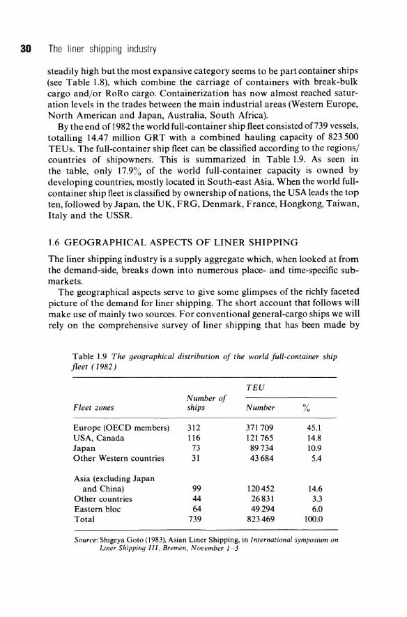
30 The liner shipping industry
steadily high but the most expansive category seems to be part container ships (see Table 1.8), which combine the carriage of containers with break-bulk cargo and/or RoRo cargo. Containerization has now almost reached saturation levels in the trades between the main industrial areas (Western Europe, North American and Japan, Australia, South Africa).
By the end of 1982 the world full-container ship fleet consisted of739 vessels, totalling 14.47 million GRT with a combined hauling capacity of 823500 TEUs. The full-container ship fleet can be classified according to the regions/ countries of shipowners. This is summarized in Table 1.9. As seen in the table, only 17.9% of the world full-container capacity is owned by developing countries, mostly located in South-east A1>ia. When the world fullcontainer ship fleet is classified by ownership of nations, the USA leads the top ten, followed by Japan, the UK, FRG, Denmark, France, Hongkong, Taiwan, Italy and the USSR.
1.6 GEOGRAPHICAL ASPECTS OF LINER SHIPPING
The liner shipping industry is a supply aggregate which, when looked at from the demand-side, breaks down into numerous place- and time-specific submarkets.
The geographical aspects serve to give some glimpses of the richly faceted picture of the demand for liner shipping. The short account that follows will make use of mainly two sources. For conventional general-cargo ships we will rely on the comprehensive survey of liner shipping that has been made by
Table 1.9 The geographical distribution of the world full-container ship fleet (1982)
TEU Number of
Fleet zones ships Number %
Europe (OECD members) 312 371709 45.1 USA, Canada 116 121765 14.8 Japan 73 89734 10.9 Other Western countries 31 43684 5.4
Asia (excluding Japan and China) 99 120452 14.6
Other countries 44 26831 3.3 Eastern bloc 64 49294 6.0 Total 739 823469 100.0
Source: Shigeya Golo (1983). Asian Liner Shipping. in International symposium on Liner Shipping III. Bremen. November 1-3

Characteristics of demand and supply 31
Lawrence (1972). For the description of container ships movements, we rely on data collected by various shipping lines and reported in the International Symposium on Liner Shipping III, Bremen, 1983.
1.6.1 The dominance of intercontinental trade
The geographical characteristic ofliner trade routes which we want to hold up in the first place, is the dominance of intercontinental trade requiring transocean shipping. From the analysis of the geography of seaborne general-cargo trades made by Lawrence (1972; chapter 6) it can be concluded that in terms of tons something like 80% of world seaborne trade in general cargo is intercontinental and 20% is intra-continental. In terms of ton-miles, and shipping demand, the dominance of intercontinental trade is apparently still more pronounced.
For container services the three main routes that link the three regions - the Far East, North America, and Europe - had been containerized almost completely by 1982. These three areas are dominantly the centres of containerized cargo traffic. They generate 91% of the containerized world trade volume. Of a total of98 million tonnes of containerized cargo in 1980,46 million, or 47%, were carried along a longitudinal belt connecting these regions. Container cargo traffic between US/Canada and UK/Continent/the West Mediterranean is estimated at 19 million tonnes or 19% of the world containerized cargo. The second largest container route is the trans-Pacific route between US/Canada and Far East/South East Asia. This trade carried 18 million tonnes, with an 18% share accordingly.
The third largest trade route is the UK/Continent/West Mediterranean to the Far East/South East Asia, with an estimated 9 million tonnes, with a 9% share. The combined total of the above three routes is 47% of the world total.
In the direction of north to south and vice versa, it is estimated that 40 million tonnes were carried, comprising 41 % of the total. This cargo was distributed:
To/from US/Canada: To/from Europe: To/from Asia:
10 million tonnes (10%) 21 million tonnes (21%) 9 million tonnes (9%)
The trade volume in the north-south direction (between developing countries) is still in its infancy and amounts to a little over 2 million tonnes, less than 2.5%.
1.6.2 The dense-route and thin-route sectors
Every pair of general-cargo ports of the world represents, in principle, a specific demand for liner services. The number of such specific demands reaches an almost astronomical figure. It is quite obvious that the number of

32 The liner shipping industry
specific liner services cannot match this figure. Even if one takes countries rather than ports, the number of potential trade routes - each pair of st:aboard countries constitutes a potential trade route - the same statement holds true: the number of direct liner shipping connections is well below the potential number of trade pairs.
Lawrence estimates the number of trade pairs that generate sufficient general cargo to support weekly sailings to be approximately 240. This is only a small fraction ofthe total number of potential trade pairs. It implies that liner services can be offered at a reasonable frequency to the majority of countries in the world only by employing a complex itinerary, in which liners call at ports of different countries. Only a few pairs of trading countries generate sufficient cargo to support weekly services. The implications of trade thinness for the design of liner services are discussed in later chapters.
The degree of concentration of the flows of general cargo is quite remarkable. According to Lawrence's calculations 60% of the total volume of general-cargo trade moves on the fifteen densest routes.
From a demand-side point of view the total liner shipping industry can thus be divided into two quite distinct sectors: the dense-trade-route sector, and the thin-trade-route sector. The former sector dominates in terms oftrade volume, while the latter sector is completely dominating in terms of numbers of routes.
1.6.3 The directional cargo balance
Another important geographical aspect is the directional balance of generalcargo movements. In terms of value it is well known that most countries show a surplus in the trade with some countries and deficits in the trade with other countries. It is unusual that the export and import value balance in each particular relation.
In terms of trade volume the general imbalance between individual trade pairs is far more pronounced. We have calculated the average 'index of imbalance' of the fifteen major general-cargo trades, which, according to Lawrence (1972), generate 60% of total general-cargo trade. The unweighted average ratio ofthe volume of cargo on the fat leg to the volume of cargo on the meagre leg comes to no less than 3.15: 1. Practically every major trade route is unbalanced to a higher or lower degree. Of the trade routes which have been subject to our cost and freight-rate investigation, accounted for in chapter 3, only a few routes were found to be fairly balanced.
1.6.4 Variability of the demand for shipping
Shipping services are not storable. If the supply of shipping capacity exceeds demand, the excess supply cannot be stored and sold again when demand exceeds supply. The generally considerable variability in demand for shipping
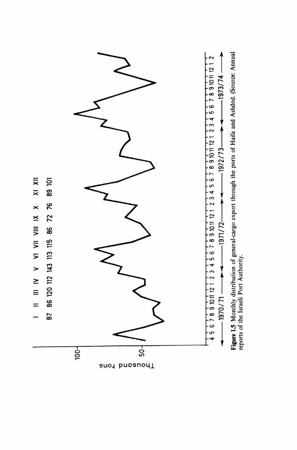
IJ) c 0 .I-
"U
C a IJ) :J
0 .s:: r
II III
IV
V
VI
VI
I VI
II IX
X
XI
XI
I
87
86 1
20 1
12 1
43 1
13 1
15
86
72
76
89 1
01
100 50
4 5
6 7
8 9
1011
12
1 2
3 4
5 6
7 8
9 10
11 1
2 1
2 3
4 5
6 7
8 9
1011
12
1 2
3 4
5 6
7 8
9 10
l'
12 1
2
• 19
7017
1 ~.
..
1971
172
.,. ..
19
7217
3 ~
"4
1973
174
----+
Fig
ure
1.5
Mon
thly
dis
trib
utio
n of
gen
eral
-car
go e
xpor
t th
roug
h th
e po
rts
of H
aifa
and
Ash
dod.
(So
urce
: A
nnua
l re
port
s of
the
Isra
eli
Po
rt A
utho
rity
.
34 The liner shipping industry
is particularly important under these conditions. Three reasons for variations in shipping demand can be distinguished.
First, there are the unpredictable, major single contingencies, which will change the cargo base of shipping services very radically, like political upheavals, changes in climate, or dramatic changes in economic policy. The Korean war and the closure of the Suez Canal are two cases in point. The latter event caused a dramatic increase in shipping requirement. The tanker tonmiles increased by approximately 15% as a consequence of the re-routing of tankers around the Cape of Good Hope.
Second, there are a large number of recurrent, but more or less random minor occurrences, like strikes and other work stoppages, weather changes, variations in production and tastes etc, that affect shipping demand.
Third, there are predictable cyclical fluctuations in demand for shipping. There is a substantial amount of seasonality in the bulk trades. Agricultural products are forthcoming during short harvest periods. Oil to Europe and North America reaches a peak during winter because of heating requirements. But seasonality also characterizes trades in general cargo. This is illustrated in the following example of monthly pattern of Israeli exports of break-bulk cargo (Fig. 1.5). The 'index of seasonality' that appears in the figure (the monthly tonnage as a percentage of the moving average of 12 months) shows that the volume of cargo in the peak month (May) was twice that of the lowest off-peak month (September).
2 Market organization: the conference system
Liner shipping stands out, together with the international airline industry, in the world economy in being almost completely cartelized in the first place as far as pricing is concerned. Unlike the airline industry, the organization of the freight rate making in the liner shipping industry is highly decentralized. Practically every longer trade route of the world is covered by a separate coalition of liner-service operators - the liner conference - which fixes the freight rates on the route concerned. This does not necessarily imply that price competition is wholly ruled out on all liner-trade routes. Outside competition from independent liners and tramps, and to a lesser extent from industrial (bulk) carriers and air freight, occurs at varying intensity. On some routes competition can be fierce occasionally. On other routes the conference members operate in 'splendid isolation'.
2.1 THE SCOPE OF THE CONFERENCE SYSTEM
There is no accurate figure available for the total number of conferences in operation. In Croner's World Directory of Liner Conferences (1976) the number listed is 341. It can be assumed that some conferences covering local short-sea trades are not included in this figure.
Anyway, conferences exist in most liner trades and in practically all intercontinental trades. The broad lines of the geographical distribution of conferences is summarized in Table 2.1. It can be noted that in the normal case a conference covers the trade in one direction only.
Membership in the conferences can vary from two to sixty-five shipping lines flying many different flags. As seen from the table the average number of members of a conference is about eleven.
The itinerary of services covered by conferences varies greatly, depending mainly on the volume oftrade generated in different trading areas, but also on political considerations. Thus, China and Indonesia are covered by conferences serving only these countries. And conference lines calling at Israeli ports will not call at any of the neighbouring ports of Arab countries. In other cases of ' thin trades' it is usual that more than one country is included in the range of a particular conference at one or both ends.
2.2 CONFERENCE ORGANIZATION AND MAIN ACTIVITIES
Liner conferences differ considerably in their organization and the scope of their activities. The conference system is not controlled by a central body like
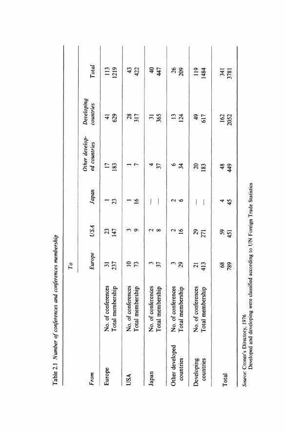
Tab
le 2
.1
Num
ber
of c
orife
renc
es a
nd c
onfe
renc
es m
embe
rshi
p
To
Oth
er d
evel
op-
Dev
elop
ing
Fro
m
Eur
ope
USA
Ja
pan
ed c
ount
ries
co
untr
ies
Tot
al
Eur
ope
No.
of
conf
eren
ces
31
23
1 17
41
11
3 T
otal
mem
bers
hip
237
147
23
183
629
1219
USA
N
o. o
f co
nfer
ence
s 10
3
1 28
43
T
otal
mem
bers
hip
73
9 16
7
317
422
Japa
n N
o. o
f co
nfer
ence
s 3
2 4
31
40
Tot
al m
embe
rshi
p 37
8
37
365
447
Oth
er d
evel
oped
N
o. o
f co
nfer
ence
s 3
2 2
6 13
26
co
untr
ies
Tot
al m
embe
rshi
p 29
16
6
34
124
209
Dev
elop
ing
No.
of
conf
eren
ces
21
29
20
49
119
coun
trie
s T
otal
mem
bers
hip
413
271
183
617
1484
Tot
al
68
59
4 48
16
2 34
1 78
9 45
1 45
44
9 20
52
3781
Sour
ce:
Cro
ner's
Dir
ecto
ry,
1976
D
evel
oped
and
dev
elop
ing
wer
e cl
assi
fied
acc
ordi
ng t
o U
N F
orei
gn T
rade
Sta
tistic
s
Market organization: the conference system 37
IA TA in the air-line industry. Nor is it under any public service obligations similar to these that bind inland 'common carriers' in most countries.
The degree of collusion between conference members varies greatly. A conference may simply comprise
informal gathering or intermittent, irregular meeting at which rates, sailings or other matters of mutual interest are arranged. These may be nothing but an informal understanding that the traffic official of one line will consult those of another whenever any rate changes are contemplated. In most cases however conferences are a formal organization with permanent officers, committees, regular or special meetings, rules and penalties. (Johnson and Huebner, 1960)
Short-sea conferences such as those covering routes between the UK and various European countries fall into the category of 'loose' or 'inactive' conferences. According to the Rochdale report: 'On the short sea routes of Western Europe, the conference arrangements have generally broken down in recent years' (HMSO, 1970). Conferences covering deep-sea trades mostly belong to the other category.
The main activities of an individual conference concern internal affairs of freight rates, supply regulation, and market division. In addition the conference system as a whole maintains a kind of order in the liner shipping industry by dividing the total market into a great number of sub-markets. Conferences define their respective ranges, thereby preventing exaggerated return-load hunting in neighbouring trading areas.
2.2.1 Conference freight rates
The great majority of the freight carried by conference members have rates fixed collectively by the conference, and which are published in rate books (tariffs). The tariff describes the articles included and specifies all the rules and regulations concerning the applicable freight rates. There are also some commodities that move at so called 'open rates'. These are commodities that face particularly strong competition from tramp shipping. The opening of rates is mainly a policy instrument to meet external competition. It is also a means of mitigating the effects of internal competition. Whenever the conflicting interests of some conference members cannot be bridged, a possible solution is to declare rates open. A request by a shipper for a rate reduction may be rejected by some conference members, while approved by others. A compromise is sometimes to declare the commodity in question as open-rate cargo. Another example is when some conferences members are suspected of granting secret rebates on freight rates of certain commodities. The other members may then demand a legalizing of internal competition by declaring these rates open (Fact Finding Investigation, 1961; pp. 154-5).
Changes in freight rates can only be made with the consensus of the
38 The liner shipping industry
conference. The shippers' interests are taken into account in as much as freight rates in the tariff cannot be changed without an advance notice. In the recommendation of the Committee of European National Shipowners' Association (CENSA) made in Brussels in October 1965, in connection with the discussion of a code of conduct in dealings between shipping conferences and shippers, it was stated that: 'As a general recommendation, where freight rate increases are contemplated, the current month plus the next two following should be given as the period of notice. Such a period of notice is, it is understood, already given by most conferences' (UNCT AD, 1970). In practice it is usual that more than 3 months elapse from the date of contemplating across-the-board rate increases, as the internal conference procedure of changing rates is quite complicated (discussed in Fact Finding Investigation, 1961; pp. 49-60 and 66-8). Changes in conference freight rates are said to be typically made in intervals of 6-12 months. The new US Shipping Act, 1984 specifies that 'rates, charges, classifications, rules, or regulations of controlled carriers, may not, without special permission of the commission, become effective sooner than the 30th day after the date of filing with the commission' (Section 9.c of the Act). Freight rates of different conferences are believed, now as before, to tend to move together. McLachlan (1963) constructed correlation indices for changes in freight rates of conferences operating on different routes. How much of this consensus regarding the conferences' listing of freight rates is borne out by our own investigation is discussed in section 3.1.
2.2.2 Do conferences monopolize the trade?
Where no competition from non-conference liners exist, nor competition from tramps or air freight, conferences may enjoy a high degree of monopoly power over the route concerned (there may still be competition from other sources of supply of the commodity). This is a situation that may prevail in some of the thin-trade routes in the world. On the dense main trading routes, one or more of these prerequisites are likely to be violated.
First, competition from the tramps. Traditionally when the bulk market was bad, tramp bulk operators would enter the liner trade, but when the market changed to the better they would make a comeback to the tramp market. During the last few years a different pattern has emerged where a number of bulk operators have established themselves in the liner market, with a declared intention to stay. They normally run fairly regular services, and are capable of combining the carriage of bulk in one direction and containers in the other. Such bulk/container combinations exist, for example, in the trade between USA/Australia, and a bulk/car carriage combination in the trade between Europe and Japan. A Neo Bulk Shipping Study (prepared for the US Department of Commerce by Harbridge House Inc., April 1972) estimated that 35-50% of import liner traffic into the USA and 50-60% of exports

Market organization: the conference system 39
moving on liners, could have been transported as neo-bulk during the period from 1967 to 1970. To take another example of the Australia-to-Europe trade, the most important commodities - by their order of value: wool, fresh fruit, food, metals - may also be carried by tramps or specialized ships.
Competition from air-transport also exists, and is particularly felt in the carriage of high-value cargo. In Israel the share of airborne cargo of the total Israeli trade measured in value was 16% in 1979, while its share measured in weight was 1 %.
The most important source of competition for the liner shipping industry can be described by the phrase: 'we look for the enemy, and the enemy is us', i.e. competition between different shipping lines (of the same conference, of nonconference, or of the same nation) offering liner services. Trans Freight Line (TFL) in the North Atlantic is a good example. Starting operation in the North Atlantic in 1976 among four other independent lines, the company had grown up to control almost 20% of the market by 1982. In fact, the company has grown so much as a 'tolerated outsider' that it has become intolerant towards competition by others and joined certain conferences to protect their interests. * Evergreen is another striking example. The company, mostly operating on routes confined to South East Asia, has grown as an independent line to a size bigger than conference members in some trades. In its turn, similar to the pattern followed by TFL, Evergreen operating as a 'tolerated outsider' in the Far Eastern Freight Conference, has been faced with a growing competition by the state-run line Yangming. The latter, acting as a complete outsider, offered a European service from March 1983 with four 1846-TEU container ships in an attempt to force its way into the closed market. It appeared that Evergreen - the outsider - could no longer avoid Yangming's growing operations and was seeking agreement with the intruder.
More generally, the three major liner routes connecting the three regions -the Far East, North America, and Europe - have increasingly been facing competition by outsiders in recent years. The weight of outsider ships in terms of TEU capacity at the end of 1982 exceeded one-third of the total on all the three key routes. On the USA/Europe and Mediterranean route, the combined TEU capacity of non-conference ships represented about 39% of the total. When both full- and part-container ships are taken into account, the share of non-conference was approximately 23% of the TEU capacity on transpacific routes in 1978, and it had gone up to 34.4% at the end of 1982. On transatlantic routes, the weight of non-conference ships, which was slightly above 20% in 1978, rose to 39% by the end of 1981. On Europe-related routes, there were practically no non-conference ships in 1978, while in 1978 non-conference ships on the Far East/Europe route represented 31 % of the total capacity offered (based on Koike, 1983).
• A speech delivered by John R. Arwood, President TFL, at the International Symposium on Liner Shipping, Bremen, Nov. 1983.
40 The liner shipping industry
2.2.3 Means of self-regulation by conferences
Conferences have employed various measures to protect themselves against the various sources of competition that threaten their existence. The threat to the conference stability comes both from within and from outside the conference; the measures of self-regulation adopted by conferences aim at safeguarding the conference system from both.
(a) Loyalty rebates to secure a stable total demand
Having defined its range in relation to other conferences, the share of a particular conference is then not completely secured. Outsiders can occasionally, or more permanently, challenge the conference lines by underbidding the freight rates fixed by the conference. Naturally it is of interest to the conference as a whole that, when given, the freight rates shippers' demand for liner services are as stable as possible. To secure 'their' cargo, liner conferences have long since found means of securing patronage of shippers. The most important one is the loyalty rebates. According to this system a rebate of the order of 10-15% is granted on a continuous basis to shippers who have signed exc1usivepatronage contracts. Still more efficient (and more controversial) is the 'deferred rebates' system, which means that shippers get the rebate, for example, on a year's freight retroactively but only provided that they have not used a non-member line or tramp at any occasion.
In the USA the system of deferred rebate has not been allowed, as it violates the anti-trust law. The Shipping Act, 1984 endorsed this prohibition. Loyalty rebates have been allowed and are still permitted by the new law. According to the new act, the conditions specifying the loyalty rebate must be published in the tariff book, and must not violate the anti-trust law. Loyalty rebates which discriminate between shippers, whether they have or have not patronised the line in question, are not allowed. (A method employed by shipping lines operating in the USA trade to discriminate among shippers is to grant quantities discount; some shippers - with larger quantities of cargo - will get lower rates than others.) An important contributory cause is mini-bridge routings that have been inaugurated by almost all carriers in the USA trade, and for practical reasons these shipments are not subject to the loyaltycontract systems. Traffic routings via Canadian ports have further weakened the loyalty-contract system. The conference inability to implement loyaltycontract systems in the face of strong competition from non-conference and their own members offering mini-bridge services, was a contributory cause to the weakening of the conference system and its replacement in some cases by a more loose organization of independent rate-setting groups.
(b) Membership restrictions
The total supply of shipping capacity is controlled by the conference in the first place by restricting the membership. Conferences that restrict entry are called
Market organization: the conference system 41
'closed conferences', and they cover most trade routes of the world except the important USA trade. Restriction on entry is not in accordance with US antitrust laws, and is not allowed in trades to and from the USA. In these trades 'open conferences' exist. Any shipping line can enter the applicable conference without the consent of existing members, provided only that the newcomer is prepared to obey all other conference rules.
(c) Market-sharing arrangements
Conference membership restrictions can only be partially effective in regulating the total supply of shipping capacity. It is difficult to check internal competition among existing conference members for a larger market share, unless further restrictions are imposed on the conference members.
All members are supposed to adhere to the fixed freight rates; the main idea of the conference system is to rule out price competition. An individual line may, however, be tempted to lower the rates because the demand facing an individual line is more elastic than the demand facing the whole conference. An individual line will increase its profit by a freight-rate reduction if the other lines stay put. This he could do by offering secret rebates, by reclassification of commodities, or by cheating in the measurement of the cargo. The incentive of an individual member in a cartel to break the cartel rules by 'cheating' in the pricing has been recognized as a main source of a built-in instability of cartels. It appears, however, that liner conferences have managed to protect themselves against this by elaborate systems of control of freight rates actually charged, and by imposing heavy penalties on conference rule-breakers.
Particularly in the USA trade, where conferences are open, self-policing devices have evolved. In these conferences a mandate to police conference members is given to a neutral body, which is eitherformed by the conference or else the conference buys these policing services from an outside concern, normally called 'policing body'. In the closed conference control over members is normally carried out by self-policing, but even here there are examples of buying 'policing body' services, as is the case with the European-Far East closed conference, which, in 1985, granted 9.5% deferred rebate (after 6 months ofloyal use of its services) to shippers. Cheating can be assumed to be practised sometimes in some trades, but not to an extent that really undermines the stability of the conferences.
The main form of competition, then, among member lines is quality, or 'service' competition. Some conferences have sought to avoid 'excessive' service competition by internal agreements to share the market to a higher or lower degree.
In cases where market-pooling arrangements are made two main forms can be distinguished, (i) quantity-pooling agreements, and (ii) revenue-pooling agreements. Output-sharing agreements allocate the total output of the conference among member lines according to some agreed formula. This is

42 The liner shipping industry
implemented in several alternative ways, e.g. allocation of 'cargo quotas', or allocation of 'sailings quotas' and 'ports quotas'.
Cargo quotas can be applied to the total trade of the conference, to specific commodities that are particularly attractive to members, or to the cargo loaded and/or unloaded in a particular port. An example of a comprehensive cargo-sharing agreement is that which applies in the Far Eastern Freight Conference (Deakin, 1973; p.65). According to this arrangement, which has been operative since 1946, the conference sets up a berthing committee which is responsible for estimating the amount of cargo expected at the next period, and on the basis of these estimates the committee allocates the cargo among the lines. Due to the administrative complications cargo quotas are in many cases confined to specific commodities like rubber in the export trade of the Far East.
Sailings quotas are applied more generally by conferences. These specify the maximum number of sailings allowed for each line on the route. Quite often this is combined with entry restrictions to particular ports; each member can make only a limited number of sailings to a specific port, or to a specific group of ports.
Quantity pooling is sometimes supplemented by a revenue-pooling arrangement. The revenue pool to be allocated can vary from 100% of the total freight revenue to a portion of the total revenue of about 40%. In early pooling agreements the quotas were determined according to a measure ofthe capacity of the ships employed by each line. A more common criterion seems now to be the quantity of cargo that has been carried by each line over a period of several years prior to the agreements (Deakin, 1973; p.67).
An important question is whether adjustments can be made in the initial shares agreed by the conference. A failure to carry the allocated quota of cargo, or to make the minimum number of sailings required by an agreement will result in a downward adjustment of the failing conference member's future market share. Upward adjustments are also made, but they seem to be more difficult for an expansive line to get through.
2.3 WHY CONFERENCES?
After the previous description of the various aspects of the conference system, this question springs to one's mind of itself: Why is practically the whole liner shipping industry thoroughly cartelized? It would not be very remarkable if liner conferences were existing in one or two liner trades; the remarkable thing is that all the hundreds of separate liner trades between all continents including all sorts of nations and geographical regions are with very few exceptions covered by conferences.
The only comparable example from another industry of the world economy is the international airline industry. A noteworthy difference is, however, that IAT A is basically an inter-governmental organization of more or less
Market organization: the conference system 43
nationalized companies, whereas the liner conferences are private cartels. An attempt to an explanation of the prevalence ofthe conference system can
start by the somewhat truistic observation that most people would like to lead a quiet life in a profitable business. Competition is seldom something that business men seek for its own sake, and already Adam Smith has noted that wherever business men of the same trade gather the possibility of fixing prices is an easily raised topic for conversation. Price cartels are by no means an unnatural form of industrial organization as far as the industrialists them-selves are concerned. .
The remarkable aspect ofliner conferences is that they are allowed and even approved of by governments in all countries, and have been so since the origin of the conference system at the end of the ninteenth century.
The first conference was formed in 1875 in the UK-Calcutta trade.* Since then conferences have spread first in the main trades at that time - between the UK (and continental Europe) and India, South East Asia, China, and Australia - and have later proliferated in all trades of the world. The rapid replacement of the sailing ships by steamships, which took place at the end of the nineteenth century, increased the carrying capacity of the world fleet quite rapidly. The steamships were both faster and bigger than the ships they replaced. The increase in supply was not matched on the demand side, and severe excess capacity of shipping services was created. A drastic and longlived decline in freight rates was inevitable. The incentive on the part of liner shipowners to get organized was particularly strong. The creation of the first conferences can be attributed to this severe slump.
Shipowners have since those days always been able to make a convincing case for the necessity and desirability of price cartels in liner shipping. The main point of the argumentation has been that in the absence of conferences freight rates would frequently be bid down to the direct handling cost 'floor'. This would be disadvantageous also for shippers, because frequent bankruptcies of shipping companies would mean that regular shipping services could not be maintained; every government consider it to be a national interest that 'vital trade connections' are not jeopardized. Several public inquiries into the conference system have by and large concurred in the shipowners' case for the liner conferences.
2.3.1 Public inquiries into the conference system and international shipping policy
Laws with a bearing on liner conferences have deep roots in the leading shipping nations. The Royal Commission on Shipping Rings was initiated in Britain in 1906 and reported in 1909. The commission's majority verdict on
*The most comprehensive discussion of the historical evolution of conferences is found in Deakin (1973).
44 The liner shipping industry
conferences was favourable. Conferences were acknowledged as a necessary form of organization for providing regular services at stable rates. It was pointed out, however, that the conference system may lead to excessive rates and oversupply; the commission recommended, as a result, that shippers should form trade associations for negotiations with conferences.
This attitude remains in present 'merchant shipping' laws in spite of post-war legislative efforts to prevent restrictive practices including the formation of price cartels in other industries. A notable attempt to take a new look at the shipping price cartels in the advent ofthe c~ntainer age was made in the report of the British committee of inquiry into shipping from 1970 (HMSO, 1970), known as the Rochdale report (after the chairman of the committee, Lord Rochdale). The committee summarized its recommendations so far as liner conferences are concerned in this way.
Members of conferences covering trade to and from the UK should collectively accept a published code of conference practice, which should contain provisions relating to the admission of new members, the publication of tariffs, the provision of information about revenues and costs to representatives of the Government and of shippers, and consultation with the Government and shippers (HMSO, 1970).
The existing form of organization qf the liner shipping industry - price cartels - was accepted.
In the USA the Alexander Committee was formed in 1912 and reported in 1914. It examined the-conference system in the light of the anti-trust laws. The conclusions of the committee were similar to those of the Royal Commission. Conferences were recognized as essential; free price competition cannot work in the liner shipping industry. As a result, liner conferences were exempt from anti-trust laws by the Shipping Act, 1916. A salient feature of USA shipping legislation is that conferences should be 'open', i.e. allow free entry.
Legal controversies have been a much more frequent problem in the US trades than anywhere else, since anti-trust laws are, generally speaking, comparatively vigorously enforced in industry as well as inland and air transportation in the United States. The new Shipping Act, 1984 was therefore welcomed by many commentators. Now the seemingly endless problems would disappear thanks to the very explicit 'anti-trust immunity' bestowed on liner shipping in USA trades.
Much less attention has so far been paid to quite another, potentially fundamental provision of the new act, which may well erode the price cartels in the future. In Section 5(b} (8)* it is stated that 'Each conference agreement must provide that any member of the conference may take independent action on any rate .. .'. In other words, although the law does not prohibit agreements
*For further details, see the Act itself(Public Law 98-237, 98th Congress). For an interpretation of the Act see Friedman and Devierno, 1984.
Market organization: the conference system 45
between conference members on freight rates, as it neither does regarding pooling of traffic or revenue, and coordination of sailings, it makes abundantly clear that it is unlawful to deny individual members the right to charge their own rates. Our interpretation of the new law is that freight rate tariffs produced by liner conferences should be regarded as a sort of list of 'recommended prices', which are issued by many different trade associations, which only serve as guidelines for individual members, and from which every member is free to deviate without fear of retaliation in any form.
Public investigations of liner conferences on a smaller scale, have been initiated by governments of other shipping nations. In general, their conclusions are similar to those of the British inquiries. While the need for conferences is acknowledged, several recommendations are usually made to restrict conference abuse. As a result, during the last 20 years, some legislation to that effect has followed in Japan, Australia, New Zealand and Canada in the form of explicit exceptions from fair trade or restrictive practice Acts. Similarly, work has been going on for some time in the EEC with a view to reconciling shipping policy with Articles 85 and 86 of the Treaty of Rome.
Private shippers' associations started to react on the conference system in the early 1950s. Various points were raised concerning the conference system in the Commission on Sea Transport of the International Chamber of Commerce. The pros and cons of the conference system were listed in an ICC brochure, which recommended that shippers should join in associations acting as counterparts to the conference, but it also gave blessing to the basic cartel system.
During the last two decades, in parallel with the formation of national policies towards conferences, international policy towards liner conferences have become a central issue. The instrument for initiating international policy towards conferences was the United Nations Conference on Trade and Development (UNCTAD). Shortly after its creation in 1964, UNCTAD established a committee on shipping, and a shipping and ports division that have been engaged in research into shipping. The growing criticism in the committee by the developing countries of the liner conferences serving their trades, made the European maritime nations group together in the Consultative Shipping Group (CSG). Two consequences of the CSG's activities were the formation of more shippers' councils in Europe, and the creation of the committee of European National Shipowners Association (CENSA).
UNCT AD being the voice of developing countries has initiated several studies on the establishment and expansion of merchant fleets of developing countries. The climax of these activities and the most influential outcome of UNCT AD's initiatives has been the 'UN Code of Conduct of Liner Conferences'. It was presented for discussion by the Group of 77' (countries in Africa, Asia and South America) at the UNCT AD conference in Santiago, and was adopted by a majority vote at the UN Diplomatic Conference in Geneva in 1974. The code convention came into effect on 6 December 1984. During these
46 The liner shipping industry
10 years intensive negotiations have taken place with the view of reaching a compromise between the main shipping nations and the interests of the majority members ofUNCTAD, the 'Group of 77'. The endorsed code in 1974 stipulated that the convention could not enter into force without the support of at least some OECD governments. This seemed assured at the Diplomatic Conference in Geneva, but subsequent events proved otherwise. The OECD countries decided that a common position on the code was required. In 1979, an agreement - Regulation EEC 954/79, commonly known as the 'Brussels Package - was produced, which sets the terms by which the OECD countries would sign the code convention. After the 'Brussels Package' was accepted by the OECD countries, the code convention was finally put into force in December 1984.
Of the many aspects covered by the code, the most important and most controversial one has been cargo-sharing formula of 40-40-20. According to this formula the division of liner cargo moving between each pair of countries by the conference lines should be: 40% carried by liners of each of the two trading countries, and 20% carried by third parties, so called cross-traders. These notorious magic numbers, according to the code convention are not inflexible, but are merely put as suggestions.
The market-sharing formula (MSF) should be viewed as an outcome of the conflict between shipping policy of nations which possess large merchant navies, and nations which do not, but have aspiration to become selfsupporting or near so in shipping. The MSF is a manifestation of this aspiration, and the conference system is chosen as the most suitable form of market organization to achieve this goal. The MSF is one step away from freedom to compete towards more protectionism of international shipping. But does it constitute in practice a real threat to the fleets of existing nations (i.e., developed nations) and to the freedom of competition, or is it merely a paper tiger?
The most important limitation to the wide applicability of the MSF is the 'Brussels Package'. The Package provides that EEC and (on the basis of reciprocity) OECD conference trades, are not subject to the MSF and the status quo is retained. This means that the majority of the liner trade between the developed countries is excluded from the code. Other considerations that limit the scope of the code are, (i) cargo carried by non-conference lines is excluded from the code, (ii) cargo transported under bilateral trade agreements is excluded, and (iii) military equipment for national defence purposes is excluded. Finally a large number of countries, and most important the USA, have refrained from signing the code convention. According to an estimate of Ross-Bell (1984),just the 'Brussels Package' limits the scope ofthe MSF to 7% of the world liner trade.
Even if this exact figure is not accepted, it is impossible to envisage how the code convention is capable of introducing a 'new order' into liner shipping. When all the qualifications that we mentioned are considered, the MSF will apply only to a small segment of the liner shipping industry.
Market organization: the conference system 47
There may be no direct threat of the code to the status quo of the international liner shipping industry, but there is an indirect one. The code is a deliberate effort to encourage more protectionism and bilateral agreements. It has awakened the aspiration of the developing countries to use their foreign trade as a base for developing their fleet - whether this is liner cargo or bulk, or whether it is carried by conference or non-conference lines. New bilateral agreements, such as that between the USA and Brazil who share equally the trade between them, have emerged. Korea, Japan and the Philippines have declared their intention to build their own fleet that will carry 40% of their foreign trade. The MSF concept has been extended to include bulk services. Some developing countries aim at carrying up to 70% of their bulk cargo in their own ships.
This development is a move towards more protectionism and nationalism of the international liner shipping industry. The aspirations of the 'have nots' are very understandable, when it is borne in mind that, (i) shipping is not just another industry; shipping is the mode by which almost all the goods essential for the support of nations are traded, and (ii) the liner shipping industry, mostly owned by the developed countries, has been characterized by absence of sufficient competition and secrecy of operations. Yet, it is impossible to see how in this case adding a wrong (to a wrong) will make things right. The criterion ofthe MSF concept is not one that is in accordance with the efficiency of the international division of labour. Of the two recent initiatives to set the terms by which conferences operate, the US Shipping Act, 1984 - which is a move towards a more liberal and competitive environment ofliner shipping -will hopefully set the example to follow by other nations pursuing a protective-nationalist policy - whether these are developing or developed countries.
2.4 CONCLUDING REMARKS
The original question whether liner conferences are beneficial or harmful for seaborne trade has latterly receded into the background, while the issue of protectionism in liner shipping has come to the front.
This is unfortunate in our view. The two issues are interrelated. The rigid protectionism which is emerging in the shipping industry is a bad thing, and so is, as we will argue in part III, the conference system in its traditional form. And the latter fosters the former tendency. In order to prevent a complete politicizing of international liner shipping, liner companies should of their own accord offer an alternative to the traditional price cartel organization of the industry rather than fight for the preservation of the 'free enterprise conference system' to quote a typically contradictory party cry by a leading shipping man.
A rather paradoxical fact is that comparatively low profits are made in liner shipping in spite of the cartelization of each trade. The low profitability in liner shipping is, in our view, not a sign of a favourably low level offreight rates but of
48 The liner shipping industry
low efficiency. In part III, in which the welfare aspects of the conference system are discussed, we show that the most probable explanation for the low profitability is that the potential monopoly profits are eliminated by costs of efforts on the part of individual lines to secure the potential high profits.
The opinion that the conferences system is a prerequisite for an orderly forwarding of general cargo trade must not remain unchallenged. We mean that the liner conferences create the need for themselves. The fixing of freight rates out ofline with the marginal costs (see part III) results in tensions which are mistakenly regarded as the justification for the price cartels, and which the conference members try to mitigate by further regulations and restrictions on competition.
At the same time we acknowledge that efficiency of operations require coordination of the scheduled services. How to combine efficient coordination of services and maintain price competition is the subject matter of part III. The US Shipping Act, 1984 is an important step towards a definition of such a role of liner services.
3 The level and structure of freight rates
3.1 THE GENERAL LEVEL OF FREIGHT RATES
3.1.1 Previous studies of the development of the general level of liner freight rates
The following is a description of the development of the general level of conference freight rates, which would agree with the general consensus.
Freight rates are fixed by the conference and are published in their tariff books. The general level of these rates is usually held unchanged for a period of 6 months, whence the conference would announce 'across-the-board' change in the level of rates, i.e. the general level of rates will rise by an equal proportional increase of the rates of all commodities. If we were to plot the general level of freight rates against time, a rising-step function shape is expected to emerge - rates are fixed at a certain level for a period of time, and then rise to a new level, with very few occasions of a fall in the level of rates. Conference freight rates are by and large 'sticky' downwards, which is attributed to the quasi-monopoly power that they possess.
There have been several attempts to substantiate this common belief. The first to mention is the single-handed attempt by McLachlan (1958) who constructed a liner freight rate index for the UK trade for the period 1946-57. McLachlan who based his index on the published conference rates and 'across the board' changes in these rates, did in fact confirm the common belief that liner rates are both stable and are almost always rising. As seen in Fig. 3.1, which compares McLachlan's UK exports index to the tramp freight rate index, liner rates show remarkable stability over the period (especially the period 1946-50), and except for slight declines of approximately 2-3% on several occasions have been consistently rising.
A major attempt to study the development of the level ofliner freight rates was made by Deakin (1973). Deakin studied the development of rates of individual commodities as well as the development of the general level of rates of the whole conference in some trades serving the UK - those with Australia and South East Asia, for the period 1948-70. His rate indices are based on the conference published rates, and except for one case (the trade UK-Australia) they are all unweighted rate indices; that is, they record the average movement of gross revenue per ton of the commodity or the conference concerned. In Figs 3.2 and 3.3 we show two of Deakin's indices for the trades UKIndia/Pakistan, and UK-Australia. The weighted index ofthe UK-Australia conference registers the weighted average movement of rates of individual
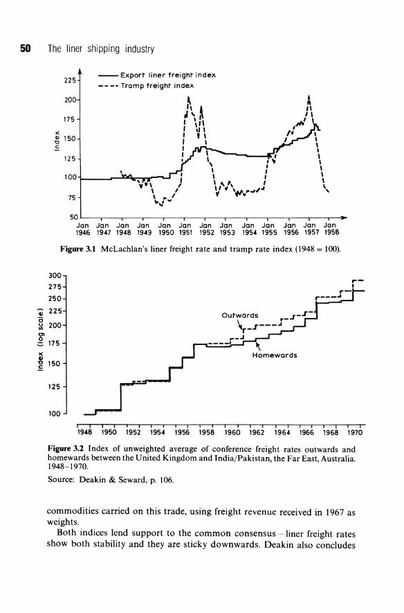
50 The liner shipping industry
GJ C u III
01 0
)( GJ '0 .:
225
200
175
>(
--Export liner freight index
-- -- Tramp freight index
~ J '\ A , \" J ,"
~ 150 I " J , c
125
75
I , I
50L-~~~---.---.--~--.---.---.--,.--, __ -.---.~ Jan Jan Jan Jan Jan Jan Jan Jan Jan Jan Jan Jan Jan 1946 1947 1948 1949 1950 1951 1952 1953 1954 1955 1956 1957 1958
Figure 3.1 McLachlan's liner freight rate and tramp rate index (1948 = 100).
300
275
250
225
200
175
150
125
100
I I I i I I i I I I i I I i I I I iii I I I i 1948 1950 1952 1954 1956 1958 1960 1962 1964 1966 1968 1970
Figure 3.2 Index of un weighted average of conference freight rates outwards and homewards between the United Kingdom and India/Pakistan, the Far East, Australia. 1948-1970.
Source: Deakin & Seward, p. 106.
commodities carried on this trade, using freight revenue received in 1967 as weights.
Both indices lend support to the common consensus -liner freight rates show both stability and they are sticky downwards. Deakin also concludes
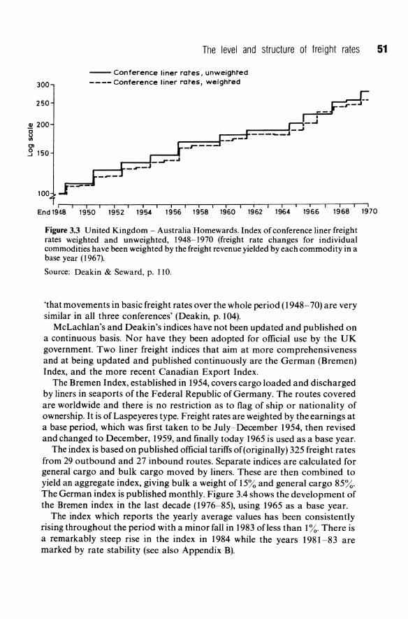
The level and structure of freight rates 51
-- Conference liner ra~es. unweigh~ed 300 ---- Conference liner ra~es, weigh~ed
250
QJ 200 --~===:j-~ ~
01
r- -----~ r-----r-r-
.3 150
100
r------f- oJ" - ...
r--_ ....... -.r- _J
ill I I I I r I I I I End 19-'.8 1950 1952 1954 1956 1958 1960 1962 1964 1966 1968 1970
Figure 3.3 United Kingdom - Australia Homewards. Index of conference liner freight rates weighted and unweighted, 1948-1970 (freight rate changes for individual commodities have been weighted by the freight revenue yielded by each commodity in a base year (1967).
Source: Deakin & Seward, p. 110.
'that movements in basic freight rates over the whole period (1948-70) are very similar in all three conferences' (Deakin, p. 104).
McLachlan's and Deakin's indices have not been updated and published on a continuous basis. Nor have they been adopted for official use by the UK government. Two liner freight indices that aim at more comprehensiveness and at being updated and published continuously are the German (Bremen) Index, and the more recent Canadian Export Index.
The Bremen Index, established in 1954, covers cargo loaded and discharged by liners in seaports of the Federal Republic of Germany. The routes covered are worldwide and there is no restriction as to flag of ship or nationality of ownership. It is of Laspeyeres type. Freight rates are weighted by the earnings at a base period, which was first taken to be luly-December 1954, then revised and changed to December, 1959, and finally today 1965 is used as a base year.
The index is based on published official tariffs of (originally) 325 freight rates from 29 outbound and 27 inbound routes. Separate indices are calculated for general cargo and bulk cargo moved by liners. These are then combined to yield an aggregate index, giving bulk a weight of 15% and general cargo 85%. The German index is published monthly. Figure 3.4 shows the development of the Bremen index in the last decade (1976-85), using 1965 as a base year.
The index which reports the yearly average values has been consistently rising throughout the period with a minor fall in 1983 of less than 1 %. There is a remarkably steep rise in the index in 1984 while the years 1981-83 are marked by rate stability (see also Appendix B).
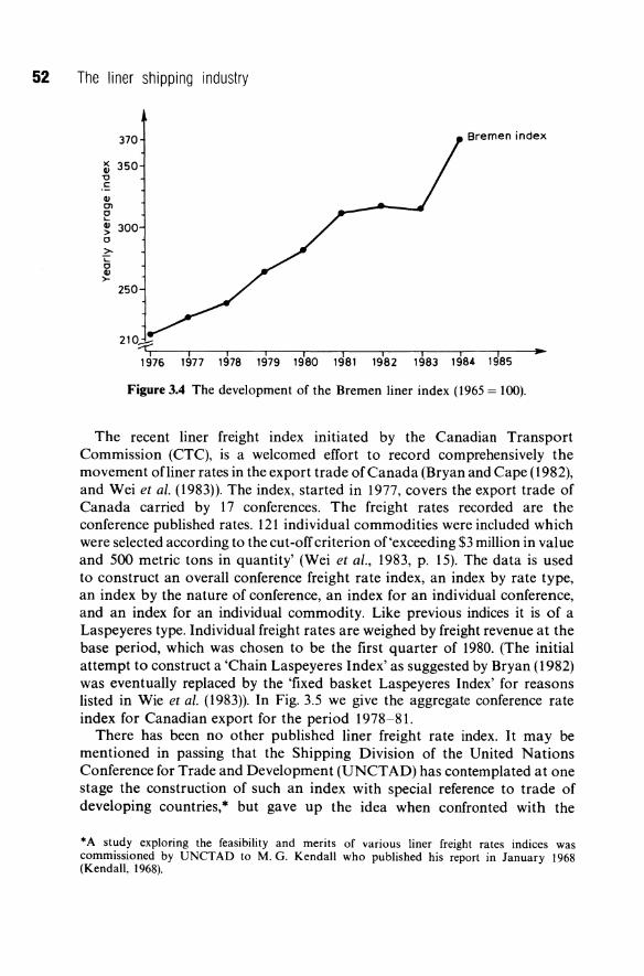
52 The liner shipping industry
370
~ 350 '0 c QJ Ol C
v 300 > c >L: c ~
250
Bremen index
Figure 3.4 The development of the Bremen liner index (1965 = 100).
The recent liner freight index initiated by the Canadian Transport Commission (CTC), is a welcomed effort to record comprehensively the movement ofliner rates in the export trade of Canada (Bryan and Cape (1982), and Wei et al. (1983)). The index, started in 1977, covers the export trade of Canada carried by 17 conferences. The freight rates recorded are the conference published rates. 121 individual commodities were included which were selected according to the cut-off criterion of'exceeding $3 million in value and 500 metric tons in quantity' (Wei et al., 1983, p. 15). The data is used to construct an overall conference freight rate index, an index by rate type, an index by the nature of conference, an index for an individual conference, and an index for an individual commodity. Like previous indices it is of a Laspeyeres type. Individual freight rates are weighed by freight revenue at the base period, which was chosen to be the first quarter of 1980. (The initial attempt to construct a 'Chain Laspeyeres Index' as suggested by Bryan (1982) was eventually replaced by the 'fixed basket Laspeyeres Index' for reasons listed in Wie et al. (1983)). In Fig. 3.5 we give the aggregate conference rate index for Canadian export for the period 1978-81.
There has been no other published liner freight rate index. It may be mentioned in passing that the Shipping Division of the United Nations Conference for Trade and Development (UNCT AD) has contemplated at one stage the construction of such an index with special reference to trade of developing countries,* but gave up the idea when confronted with the
*A study exploring the feasibility and merits of various liner freight rates indices was commissioned by UNCTAD to M. G. Kendall who published his report in January 1968 (Kendall, 1968).
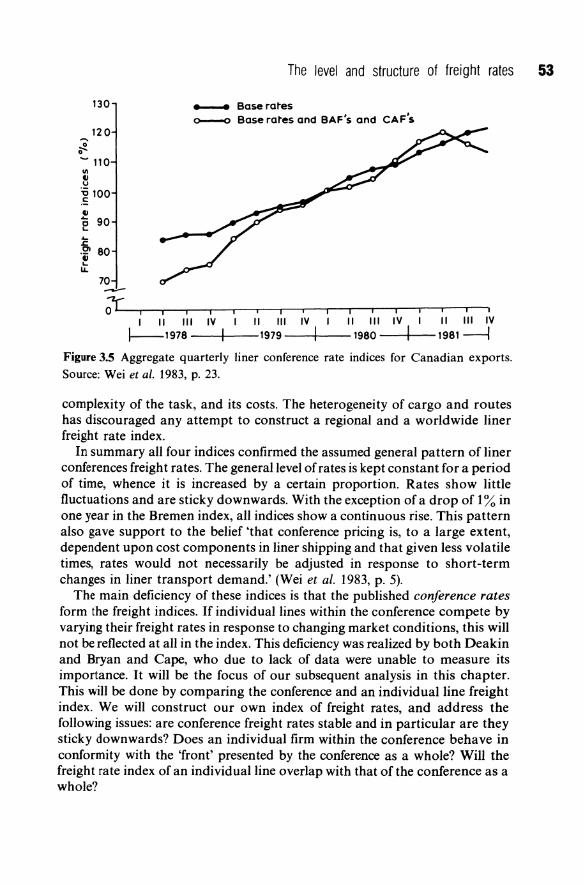
..... o
0"-
130
120
~ 110 1/1
8 .~ 100
GJ "0 90 L.
..... ~ 'ii 80 L. U.
70
The level and structure of freight rates 53
_ Basera~es
0--0 Base ra~es and BAF's and CAF's
I i I I I I II III IV II III IV II III IV II III IV
1-1978---+1--1979---+-1--1980--+-1 -1981---i
Figure 3.5 Aggregate quarterly liner conference rate indices for Canadian exports.
Source: Wei et al. 1983, p. 23.
complexity of the task, and its costs. The heterogeneity of cargo and routes has discouraged any attempt to construct a regional and a worldwide liner freight rate index.
In summary all four indices confirmed the assumed general pattern of liner conferences freight rates. The general level of rates is kept constant for a period of time, whence it is increased by a certain proportion. Rates show little fluctuations and are sticky downwards. With the exception of a drop of 1 % in one year in the Bremen index, all indices show a continuous rise. This pattern also gave support to the belief 'that conference pricing is, to a large extent, dependent upon cost components in liner shipping and that given less volatile times, rates would not necessarily be adjusted in response to short-term changes in liner transport demand.' (Wei et al. 1983, p. 5).
The main deficiency of these indices is that the published conference rates form the freight indices. If individual lines within the conference compete by varying their freight rates in response to changing market conditions, this will not be reflected at all in the index. This deficiency was realized by both Deakin and Bryan and Cape, who due to lack of data were unable to measure its importance. It will be the focus of our subsequent analysis in this chapter. This will be done by comparing the conference and an individual line freight index. We will construct our own index of freight rates, and address the following issues: are conference freight rates stable and in particular are they sticky downwards? Does an individual firm within the conference behave in conformity with the 'front' presented by the conference as a whole? Will the freight rate index of an individual line overlap with that of the conference as a whole?
54 The liner shipping industry
Do rates of individual commodities move in parallel, so that 'across-theboard' changes in rates accord well with the actual rate changes that have taken place, or do actual freight rates of individual commodities move in a different manner?
To answer these questions we construct a liner shipping freight-rate index. This is done for two shipping trade routes: the route FRG (Hamburg/Bremen Ports) to Israel, controlled by the conference CONISCON, and the route west coast of Italy/Sicily and Adriatic ports to North Atlantic ports range, controlled by the conference WINAC. For the first route two indices of the general level of rates over the route, for the period 1975-85, are constructed. One for the whole conference, and a second one for a particular shipping line operating within the conference. For the second trade route, commodity indices are constructed of the three main commodities moving on this trade, for the period 1979-85.
3.1.2 Liner freight rates indices on the FRG to Israel trade route
The trade route selected - FRG to Israel which covers a distance of 3650 miles - constitutes a part of the larger trade zone of north-west Europe to the Mediterranean. The latter is served by more than twenty lines offering more than 25000 containers per month in various combinations of sea and land. Out of these twenty companies only nine call at Israeli ports, offering 10000 containers per month via more than twenty-five different ships. Five out of these nine companies have colluded by forming closed conferences, while the remaining four act as independents (Matthews, 1984).
The part of this trade that is studied here -(FRG to Israel) is served by five shipping lines offering approximately 6700 containers per month. Three of these are organized in a closed conference called CONISCON. They include Zim (Israel), ONOL (FRG), and KNSM (the Netherlands). Together they offer 45% of the total capacity offered on the route, Zim having 63% of the capacity offered by the conference. Of the cargo moved over this route 80% is liner cargo, which mostly consists of finished and semi-finished manufactured goods.
Conferences can best be described as 'price cartels'. The member shipping lines coordinate the freight rates they charge and publish a uniform tariff for all the services provided by them. In other respects, conferences may vary in their degree of control of member lines. They sometimes form a loose organization for the sole purpose of coordinating rates (especially on short sea hauls), and at the other extreme they may exercise tight control over members to the extent of sharing revenue according to some agreed formula. Another important distinction is between 'closed' and 'open' conferences. Closed conferences do not admit free entry to the conference, while open conferences allow free entry. All conferences serving the USA trade are open conferences by the anti-trust law.

The level and structure of freight rates 55
The CONISCON is an example of a conference with tight control over members. It is a closed conference consisting of just three shipping lines (of different nations) operating on the basis of a 'revenue pool', i.e. of sharing revenue. At the same time the conference faces strong competition from the three independent firms (or 'outsiders') that offer more than 50% of the total shipping capacity on the route. The intriguing question is whether the conference can sustain or even raise freight rates when faced with competition from the 'independents'. Can the conference avoid lowering its published freight rates when faced by a situation of excess capacity and strong competition? To answer this question we construct a conference freight-rate index, which is based on the published rates of the conference.
(a) The conference freight rate index
The unit of account for the construction of the index is a standard container of a dimension of 20 x 20 x 8 feet, also called a Twenty-Foot Equivalent Unit (TEU). The freight-rate index is calculated per TEU of a representative commodity mix. CONISCON publishes twenty-nine classes of rates in its tariff, called 'official scale of rates'. Out of this list we have chosen twelve classes of rates, which cover 80% of the total trade. A representative TEU, then, consists of a mix of these twelve commodity groups, being weighted by the revenue share of each class. The conference rates that we use are the 'basic rates' that are quoted to all shippers, under the category 'non-contractors', and prior to any rebates an individual line is allowed to get by mutual agreement. To this basic charge we have added surcharges when applicable (such as the Yom-Kippur war surcharge applicable since 1973), and fuel surcharges.
A freight-rate index compares the average (weighted) of a set of freight-rate relatives; that is, a set of rates in period t is being compared to a corresponding set of rates at some other period. The weights that are assigned to the freight rates are their respective quantities or revenue. They can be fixed at a reference period in the past, in which case the index is of a Laspeyeres type, or they can be fixed at a reference period of the current year in which case the resulting index is a Paasche index. Weights can also change continuously, in which case the index is a 'chain index' - of a Laspeyeres type if last year's weights are used, or of a Paasche type if current weights are used. (For a general discussion on indices see Allen, 1975)
The index we construct is of Laspeyeres type with fixed weights of the base period, which is 1975. The weights used are the revenue share of each commodity group in 1975:
ptWO p --
L - pOWo
where pt is a vector offreight rates Pj (i = 1, ... , 12) at time t
WO is a vector of revenue shares Wj (i = 1, ... , 12) at base year
(3.1 )
PL is a Laspieres price index using a TEU as a unit of measurement
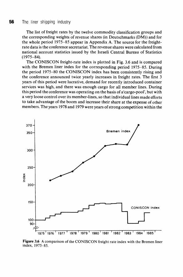
56 The liner shipping industry
The list of freight rates by the twelve commodity classification groups and the corresponding weights of revenue shares (in Deutschmarks (DM)) and for the whole period 1975-85 appear in Appendix A. The source for the freightrate data is the conference secretariat. The revenue shares were calculated from national account statistics issued by the Israeli Central Bureau of Statistics (1975-84).
The CON IS CON freight-rate index is plotted in Fig. 3.6 and is compared with the Bremen liner index for the corresponding period 1975-85. During the period 1975-80 the CONISCON index has been consistently rising and the conference announced twice yearly increases in freight rates. The first 3 years of this period were lucrative, demand for recently introduced container services was high, and there was enough cargo for all member lines. During this period the conference was operating on the basis of a'cargo-pool', but with a very loose control over its member-lines, so that individual lines made efforts to take advantage of the boom and increase their share at the expense of other members. The years 1978 and 1979 were years of strong competition within the
370
350
300
250
200
150
100 90-
Bremen index
CONISCON index
~975 1 1976 i 1977 i 1978 i 1979 i 1980 I 1981 i 1982 i 1983 I 1984 i 1985 I
Figure 3.6 A comparison of the CONISCON freight rate index with the Bremen liner index, 1975-85.

The level and structure of freight rates 57
conference (more on this in section (b)), where each line wanted a bigger bite in the market. This eventually led members to agree to switch from a 'cargo-pool' to a 'revenue pool' agreement by which revenue is shared among members according to an agreed formula and accounts are settled by the conference periodically. The conference also took a decision to tighten the control over members. All this turmoil, while expected to be reflected in individual lines' rate indices (section (b)), are not reflected at all in the conference freight-rate index! During the years 1978-80 the conference index was rising. The internal competition did not induce the conference to lower freight rates. Rather, the conference has presented a unified front to the outsiders, pushing freight rates further up. The local boom in Israel and the general recovery of world economy in the years 1982-83 were expected to cause a further rise in the general level of rates. But against this increase in demand, competition by outsiders intensified, and tipped the balance. In 1982 a newly established Israeli company ISCONT joined the other two outsiders - the German CIS and the British BORCHARD. The conference responded by slightly lowering the level of rates. The drastic measures taken by the Israeli Government to curtail imports in 1983 in combination with the new capacity offering finally stirred a 'cut-throat' competition between the conference and the outsiders. In 1983 the index dropped from 144 to 90 and stayed at that level during the first half of 1984. The next scenario is quite inevitable: all shipping lines serving the route have colluded and agreed on a coordinated policy, which included a reallocation of cargo between the conference and the outsiders and an agreement to raise rates. 'Order' was restored. In the second half of 1984 the freight-rate index began to rise and by 1985 it had reached the same level that prevailed 10 years ago.
The comparison with the Bremen index shows that the similarities lasted as long as the CONISCON index was rising between 1975 and 1980. Thereafter the two indices diverge in their directions. In particular in 1984 the Bremen index shows a steep rise while the CONISCON index is at rock bottom.
The CONISCON general level of rates is not sticky downwards. Conferences, like any other industrial firm, respond to outside competition by lowering rates. The specificity of the liner trade was again demonstrated, and the futility of constructing a worldwide liner index is an inevitable outcome. In contrast to the worldwide competitive tramp market, liner services are specific in time and space, and different route characteristics will lead to entirely different movement of the general level of freight rates.
(b) A freight rate index of an individual firm within the coriference
A true freight-rate index is one that records the actual freight rates that were made by shippers to the shipping lines. Are these charges identical to the rates published by the conference? Do member shipping lines adhere bluntly to the rate policy set by the conference, or will they, when faced with competition, like
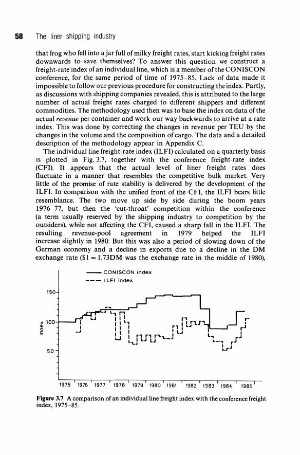
58 The liner shipping industry
that frog who fell into ajar full of milky freight rates, start kicking freight rates downwards to save themselves? To answer this question we construct a freight-rate index of an individual line, which is a member of the CONISCON conference, for the same period of time of 1975-85. Lack of data made it impossible to follow our previous procedure for constructing the index. Partly, as discussions with shipping companies revealed, this is attributed to the large number of actual freight rates charged to different shippers and different commodities. The methodology used then was to base the index on data of the actual revenue per container and work our way backwards to arrive at a rate index. This was done by correcting the changes in revenue per TEU by the changes in the volume and the composition of cargo. The data and a detailed description of the methodology appear in Appendix C.
The individual line freight-rate index (ILFI) calculated on a quarterly basis is plotted in Fig. 3.7, together with the conference freight-rate index (CFI). It appears that the actual level of liner freight rates does fluctuate in a manner that resembles the competitive bulk market. Very little of the promise of rate stability is delivered by the development of the ILFI. In comparison with the unified front of the CFI, the ILFI bears little resemblance. The two move up side by side during the boom years 1976-77, but then the 'cut-throat' competition within the conference (a term usually reserved by the shipping industry to competition by the outsiders), while not affecting the CFI, caused a sharp fall in the ILFI. The resulting revenue-pool agreement in 1979 helped the ILFI increase slightly in 1980. But this was also a period of slowing down of the German economy and a decline in exports due to a decline in the DM exchange rate ($1 = 1.73DM was the exchange rate in the middle of 1980),
-- CONISCON index
--- I LFI index
150
.... >(100+-..... QI o ~
50
1975 1976 1977 1978 1979 1980 1981 1982 1983 1984 1985
Figure 3.7 A comparison of an individual line freight index with the conference freight index, 1975-85.
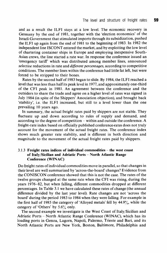
The level and structure of freight rates 59
and as a result the ILFI stays at a low level. The economic recovery in Germany by the end of 1981, together with the 'election economics' of the Israeli Government that stimulated imports through its subsidization, pushed the ILFI up again from the end of 1981 to the beginning of 1983. In 1982 the independent line ISCONT entered the market, and by exploiting the low level of chartering container ships in Europe and employing inexpensive SouthAsian crews, the line started a rate war. In response the conference issued an 'emergency tariff' which was distributed among member lines, announced selective reductions in rate and different percentages, according to competitive conditions. The member lines within the conference had little fat left, but were forced to be stripped to their bones.
Rates by the second half of 1983 began to slide. By 1984, the ILFI reached a level that was less than half its peak level in 1977, and approximately one-third of the CFI peak in 1981. An agreement between the conference and the outsiders to share the trade and agree on a higher level of rates was signed in July 1984 (in spite of the Shippers' Association objection), and brought back 'stability', i.e. the ILFI increased, but still to a level lower than the one prevailing 10 years ago.
In summary, the actual freight rates paid by shippers are not stable. They fluctuate up and down according to rules of supply and demand, and according to the degree of competition - within and outside the conference. A freight-rate index based on officially published conference-rates does not truly account for the movement of the actual freight rates. The conference index shows much greater rate stability, and is different in both direction and magnitude to the movement of the actual freight rates paid by shippers.
3.1.3 Freight rates indices of individual commodities - the west coast of Italy/Sicilian and Adriatic Ports - North Atlantic Range Conference (WINAC)
Do freight rates of individual commodities move in parallel, so that changes in their level are well summarized by 'across-the-board' changes? Evidence from the CONISCON conference showed that this is not the case. The rates of the twelve groups changed at the same rate when the CFI was rising, during the years 1976-82, but when falling, different commodities dropped at different percentages. In Table 3.1 we have calculated these rates of change (the annual difference divided by the last year level). Rate changes are not 'across the board' during the period 1983 to 1984 when they were falling. For example in the first half of 1985 the category of 'Alloyed metals' fell by 44.9%, while the category of 'Others' by 5.6% only.
The second example we investigate is the West Coast of Italy/Sicilian and Adriatic Ports - North Atlantic Range Conference (WINAC), which has its loading ports in Genoa, Lagorn, Napoli, Palermo, Trieste and Bari, and its North Atlantic Ports are New York, Boston, Baltimore, Philadelphia and

Tab
le 3
.l F
reig
ht r
ates
cha
nges
of t
he C
ON
/SC
aN
Cm
ifer
ence
s (r
ates
of a
nnua
l ch
ange
s. i
n pe
rcen
tage
s)
1976
19
77
1978
19
79
1980
19
81
1982
19
83
1984
19
85
/ II
/
II
/
Foo
d A
cros
s-th
e-bo
ard
chan
ges
in f
reig
ht r
ates
-1
9
-20
.0
0 -0
.7
17.0
C
hem
ical
s -8
.0
-22
.0
0 -1
2.0
17
.0
Pha
rmac
euti
cal
and
cosm
etic
s -1
8.0
-3
0.0
0
3.7
16.3
Pl
asti
c an
d ru
bber
-1
9.0
-2
0.6
0
4.9
17.2
T
extil
e an
d le
athe
r -
23.3
-2
8.7
0
4.9
16.3
P
aper
and
woo
d -1
0.0
-3
0.4
0
4.1
18.0
B
uild
ing
mat
eria
ls
-37
.0
-15
.8
0 -1
.8
17.3
A
lloye
d m
etal
s -4
4.9
-3
5.6
0
5.6
17.8
M
achi
nery
and
too
ls
13.2
-
35.3
0
5.6
17.8
M
otor
car
s -2
5.6
-1
6.6
0
16.l
17.8
C
onsu
mer
goo
ds
-23
.9
-23
.3
0 1.
1 17
.2
Oth
ers
-5.6
-2
6.0
0
3.7
17.8
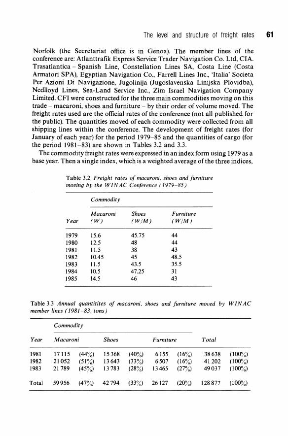
The level and structure of freight rates 61
Norfolk (the Secretariat office is in Genoa). The member lines of the conference are: Atlanttrafik Express Service Trader Navigation Co. Ltd, CIA. Trasatlantica - Spanish Line, Constellation Lines SA, Costa Line (Costa Armatori SPA), Egyptian Navigation Co., Farrell Lines Inc., 'Italia' Societa Per Azioni Di Navigazione, Jugolinija (Jugoslavenska Linijska Plovidba), Nedlloyd Lines, Sea-Land Service Inc., Zim Israel Navigation Company Limited. CFI were constructed for the three main commodities moving on this trade - macaroni, shoes and furniture - by their order of volume moved. The freight rates used are the official rates of the conference (not all published for the public). The quantities moved of each commodity were collected from all shipping lines within the conference. The development of freight rates (for January of each year) for the period 1979-85 and the quantities of cargo (for the period 1981-83) are shown in Tables 3.2 and 3.3.
The commodity freight rates were expressed in an index form using 1979 as a base year. Then a single index, which is a weighted average of the three indices,
Table 3.2 Freight rates oj macaroni. shoes and Jurniture moving by the WINAC ConJerence (1979-85)
Commodity
Macaroni Shoes Furniture Year (W) (W/M) (W/M)
1979 15.6 45.75 44 1980 12.5 48 44 1981 11.5 38 43 1982 10.45 45 48.5 1983 11.5 43.5 35.5 1984 to.5 47.25 31 1985 14.5 46 43
Table 3.3 Annual quantitites oj macaroni. shoes and Jurniture moved by WINAC member lines (1981-83. tons)
Commodity
Year Macaroni Shoes Furniture Total
1981 17115 (44%) 15368 (40%) 6155 (16%) 38638 (100%) 1982 21052 (51%) 13643 (33%) 6507 (16%) 41202 (100%) 1983 21789 (45%) 13 783 (28%) 13465 (27%) 49037 (100%)
Total 59956 (47%) 42794 (33%) 26127 (20%) 128877 (100%)

62 The liner shipping industry
Table 3.4 Commodity indices and a weighted average index of the WINAC Conference (1979-85)
WINAC indices Weighted
Year Macaroni Shoes Furniture averaged index
1979 100 100 100 100 1980 80.13 104.92 100 97.71 1981 73.72 83.06 97.73 85.0 1982 65.99 98.36 110.23 94.34 1983 73.72 95.08 80.68 86.01 1984 67.31 103.28 70.45 85.58 1985 92.95 100.55 97.73 97.97
was constructed. The weights used were the quantities moved by the conference during the whole period of 1981-83 (macaroni 47%, shoes 33%, furniture 20%). These indices are summarized in Table 3.4, and Fig. 3.8.
The WINAC indices do fluctuate quite widely. For example, the index for furniture fell by nearly 40% during 1983 and 1984 and rose again by nearly 40% during 1985. The weighted-average index also shows fluctuation during
>< CLJ "0 C
110
100
\ \
90
80
70
60 ;:;..c
I 1979
\ \ \ \
\ ~ ,
I 1980
.... , "0-. ,
I 1981
, " " " '0'
I 1982
I 1983
I 1984-
0- - -0 Macaroni 0-·_·0 Shoes 0---0 Furniture •........• Weighted average
index
Figure 3.8 Commodity indices and a weighted average index of WINAC Conference, 1979-85.
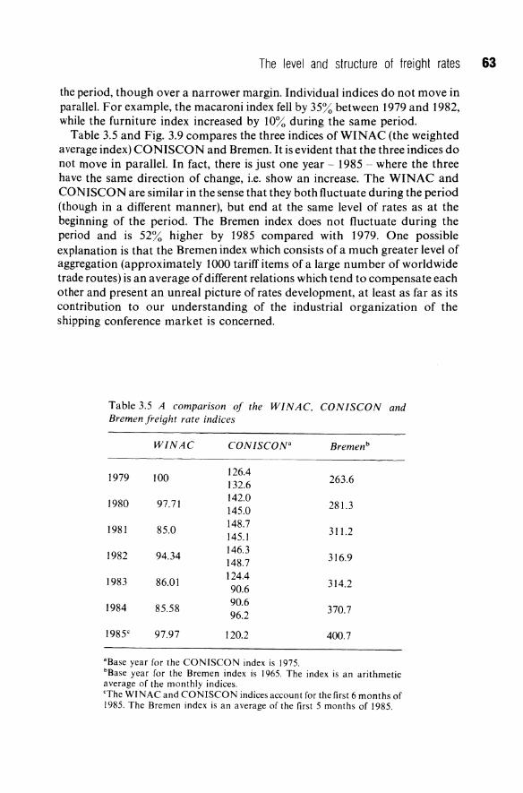
The level and structure of freight rates 63
the period, though over a narrower margin. Individual indices do not move in parallel. For example, the macaroni index fell by 35% between 1979 and 1982, while the furniture index increased by 10% during the same period.
Table 3.5 and Fig. 3.9 compares the three indices ofWINAC (the weighted average index) CONISCON and Bremen. It is evident that the three indices do not move in parallel. In fact, there is just one year - 1985 - where the three have the same direction of change, i.e. show an increase. The WINAC and CONISCON are similar in the sense that they both fluctuate during the period (though in a different manner), but end at the same level of rates as at the beginning of the period. The Bremen index does not fluctuate during the period and is 52% higher by 1985 compared with 1979. One possible explanation is that the Bremen index which consists of a much greater level of aggregation (approximately 1000 tariff items of a large number of worldwide trade routes) is an average of different relations which tend to compensate each other and present an unreal picture of rates development, at least as far as its contribution to our understanding of the industrial organization of the shipping conference market is concerned.
Table 3.5 A comparison of the WINAC, CONISCON and Bremen freight rate indices
WINAC CaNIS CON" Bremenb
1979 100 126.4
263.6 132.6
1980 97.71 142.0
281.3 145.0
1981 85.0 148.7 145.1 311.2
1982 94.34 146.3
316.9 148.7
1983 86.01 124.4 90.6 314.2
1984 85.58 90.6
370.7 96.2
1985C 97.97 120.2 400.7
aBase year for the CONISCON index is 1975. bBase year for the Bremen index is 1965. The index is an arithmetic average of the monthly indices. cThe WINAC and CONISCON indices account for the first 6 months of 1985. The Bremen index is an average of the first 5 months of 1985.

400
350
300 -.--;I' .;
", ",
/ /
/ ._---.----e"
/. .... " ..... Bremen index
.....
~ 250 u c
200
150
100
75
CONISCON index
-------_------.J:==~~~- WINAC index
~L-----'------r-----'-----~------.------r-----.~ 1979 1980 1981 1982 1983 1984 1985 I )0
Figure 3.9 A comparison of the WINAC, CONISCON, and Bremen freight-rate indices, 1979-85.
Table 3.6 A comparison of the I LF I to the spot shipment of grain index
Index
Freight rate per ton of grain, US-Rotterdam Spot grain index, 1LFl,
Year ($) U S-Rotterdam Germany-I srael
1975 5.43 100 100 1976 5.95 109.6 104.1 1977 5.06 93.2 115.3 1978 7.01 129.1 100.1 1979 13.70 252.3 67.8 1980 17.73 326.5 74.15 1981 13.55 249.5 79.4 1982 8.46 155.8 100.3 1983 8.23 151.5 85.1
Sources: The Grain Freight index: lhe Public L"dyer; COllltllodil\' Week. ILFI: Arithmetic Average of the quarterly ILFI index. .

The level and structure of freight rates 65
3.1.4 A comparison of a liner and a dry-bulk freight rate index
How do liner freight rates fluctuate in comparison with the rate fluctuations in the competitive bulk market? We now compare the ILFI to the spot freightrate index of grain shipment from the USA to Rotterdam during the period 1975-83. The annual averages of the ILFI (which smooths the quarterly fluctuations that occur within the year) and the spot grain index (SGI) are shown in Table 3.6 and Fig. 3.10.
Freight rates in the bulk market fluctuate much more widely. This common knowledge still holds true. In the competitive bulk market change in freight rate is the main instrument that clears the market. In the liner shipping market greater reliance is made on adjustments in capacity offered to correct for changes in supply and demand that have taken place.
The two indices do not follow the same pattern. In particular the years 1979 and 1980 were boom years for bulk shipping while for liner shipping, in the case investigated, these were years of depressed market conditions.
A Summary
Some of the dust covering behaviour of conferences has been cleared. The answers to the questions posed at the beginning of this section are:
x III 'C C
350
300
250
200
150
100
50 -r:
0---0 Spot grain index
•• --•• 1 LFI index
1
1975 1
1976 1977 1
1978 1979 i
1980
.--_0""'"
i 1981
." 0 ___
",. ...... -0
i
1982 I'"
1983
Figure 3.10 A comparison of the ILFI to the spot shipment of grain index, 1975-83.
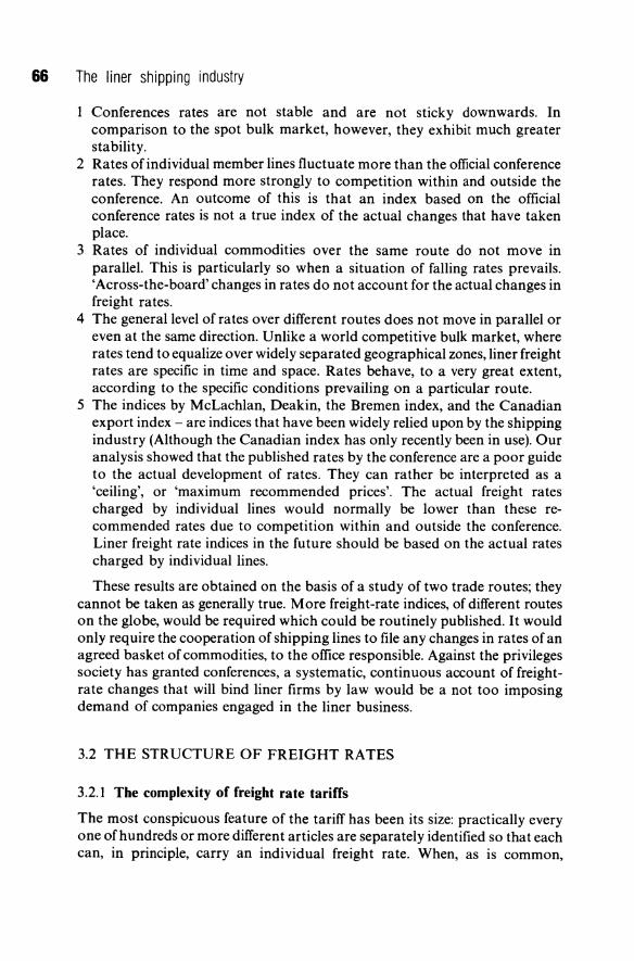
66 The liner shipping industry
Conferences rates are not stable and are not sticky downwards. In comparison to the spot bulk market, however, they exhibit much greater stability.
2 Rates of individual member lines fluctuate more than the official conference rates. They respond more strongly to competition within and outside the conference. An outcome of this is that an index based on the official conference rates is not a true index of the actual changes that have taken place.
3 Rates of individual commodities over the same route do not move in parallel. This is particularly so when a situation of falling rates prevails. 'Across-the-board' changes in rates do not account for the actual changes in freight rates.
4 The general level of rates over different routes does not move in parallel or even at the same direction. Unlike a world competitive bulk market, where rates tend to equalize over widely separated geographical zones, liner freight rates are specific in time and space. Rates behave, to a very great extent, according to the specific conditions prevailing on a particular route.
5 The indices by McLachlan, Deakin, the Bremen index, and the Canadian export index - are indices that have been widely relied upon by the shipping industry (Although the Canadian index has only recently been in use). Our analysis showed that the published rates by the conference are a poor guide to the actual development of rates. They can rather be interpreted as a 'ceiling', or 'maximum recommended prices'. The actual freight rates charged by individual lines would normally be lower than these recommended rates due to competition within and outside the conference. Liner freight rate indices in the future should be based on the actual rates charged by individual lines.
These results are obtained on the basis of a study of two trade routes; they cannot be taken as generally true. More freight-rate indices, of different routes on the globe, would be required which could be routinely published. It would only require the cooperation of shipping lines to file any changes in rates of an agreed basket of commodities, to the office responsible. Against the privileges society has granted conferences, a systematic, continuous account of freightrate changes that will bind liner firms by law would be a not too imposing demand of companies engaged in the liner business.
3.2 THE STRUCTURE OF FREIGHT RATES
3.2.1 The complexity of freight rate tariffs
The most conspicuous feature of the tariff has been its size: practically every one of hundreds or more different articles are separately identified so that each can, in principle, carry an individual freight rate. When, as is common,
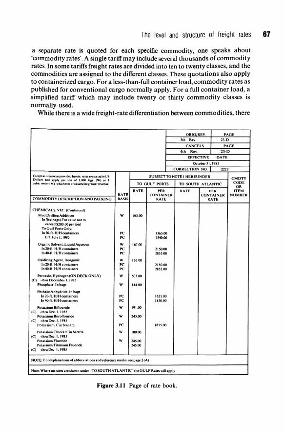
The level and structure of freight rates 67
a separate rate is quoted for each specific commodity, one speaks about 'commodity rates'. A single tariff may include several thousands of commodity rates. In some tariffs freight rates are divided into ten to twenty classes, and the commodities are assigned to the different classes. These quotations also apply to containerized cargo. For a less-than-full container load, commodity rates as published for conventional cargo normally apply. For a full container load, a simplified tariff which may include twenty or thirty commodity classes is normally used.
While there is a wide freight-rate differentiation between commodities, there
ORIGjREV. PAGE
5lh Rev. 23-D
CANCELS PAGE
4th Rev. 23·0 EFFECTIVE DATE
Oclober31.1985
CORRECTION NO. I 2223
E:\cepl as otherwise provided herein, ratesare slated in US SUBJECT TO NOTE I HEREUNDER CMDTY Dollars and apply per Ion of 1,000 Kgs-. (W) or I cubic meter (M) whichever produces the greater revenue. TO GULF PORTS TO SOUTH ATLANTIC CODE
OR RATE PER RATE PER ITEM
RATE CONTAINER CONTAINER NUMBER COMMODITY DESCRIPTION AND PACKING BASIS RATE RATE
CHEMICALS, VIZ.: (Conlinucd)
Mud Drilling Additives W 163.00 In nexibags (For value not to
exceed S200.00perton) To Gulf Ports Only: In 20-ft. H/H containers PC 1365.00
Elf. July I, 1985 PC 1540.00
Organic Solvent. Liquid Aqueous W 167.00 In 20-ft. H/H containers PC 2150.00 In 4O-ft. H/H containers PC 2855.00
Oxidizing Agent,lnorganic W 167.00 In 2O-ft. H/H containers PC 2150.00 In 4O-ft. H/H containers PC 2855.00
Peroxide. Hydrogen (ON DECK ONLY) W 503.00 (C) ·lhruDecember 1.1985
Phosphate,ln bags W 144.00
Phthalic Anhydride. In bags In 2O-ft. H/H containers PC 1625.00 In 4O-fl:. H/H containers PC 1850.00
Potassium Biflouride W 191.00 (C) ·'hruDec.I,1985
Potassium Boroflouride W 245.00 (C) -lhru Dec. I. 1985
Potassium Carbonate PC 1855.00
Potassium Chlorate. in barrels W 180.00 (C) -lhruDec.I,1985
Potassium Fluoride W 245.00 Potassium Titanium Fluoride 245.00
(C) -lhru Dec. I, 1985
NOTE: For explanations of abbreviations and reference marks. see page 2 (A)
Note: Where no ralesare shown under "TO SOUTH ATLANTIC" the GULF Rates will apply
Figure 3.11 Page of rate book.
68 The liner shipping industry
is very little differentiation between ports. The tariff often contains a classification of the ports included in the conference range into 'base ports' to which 'base rates' apply and 'outports' to which surcharges apply.
The conferences (excluding USA) normally issue two different tariffs - for non-contractors and contractors. The tariff issued for non-contractors applies equally to all shippers, but is different to the agreed tariff for contractors, i.e. for shippers who enter a long-term agreement with the conference. In the latter case different shippers will be quoted different tariffs. In Fig. 3.11 a page in a typical tariff is reproduced as a concrete illustration.
By all recent experience, it is the volume (measurement capacity) which is the capacity constraint that is binding in liner shipping. However, the freightrate tariffs issued by liner conferences do not adhere to this fact. The base for quoting freight rates of individual commodities is not standardized. Rates of individual commodities are expressed in mainly three different ways.
1 Per weigh t ton (W). 2 Per measurement ton (M). 3 Per weight ton or measurement ton, whichever gives the higher revenue
(WjM).
(A fourth type is ad valorem rates-all or part of the freight rate is paid in proportion to the value of the goods.)
The units of measurment of the different bases can, in addition, vary. A weight ton is usually defined as either a metric ton (1000 kg) or a 'long ton' (1016 kg). A measurement ton used to be commonly defined as 40 cubic feet (in some trades 50 cubic feet), or else, as is usually the case today, as 1 cubic meter, i.e., 35.5 cubic feet. A commodity that is being charged on a weight basis will pay according to its weight irrespective of the volume it occupies. A commodity that pays per volume will do so irrespective of its weight.
Even in the present container age, freight rates are sometimes quoted per weight ton, although it is well known that so far as general cargo is concerned a container is full when its total volume is occupied, and the holding capacity of a container ship is exhausted by container number rather than cargo weight.
Tradition is probably the main explanation for this practice, but also the fact that for less-than-full container loads, the weight of a shipment is often easier to determine than its volume. In this connection something could be mentioned about the traditional way of cargo measurements.
Digression 1: The 'pivot unit' system of cargo summation
It is true that thinking in terms of cargo volume has gained wide currency in the liner shipping industry in the wake of containerization for most other purposes than freight rating. The traditional practice of cargo measurement used to be based on a double-unit system - weight or volume, and almost from the beginning of shipping 'pivot unit' systems of freight charging are known.
The level and structure of freight rates 69
Especially when the ratio of a ship's volume capacity to dead-weight capacity is in the range of the average stowage factor of the commodities moving on the route concerned, it is usual to charge heavy (dense) cargo on the basis of weight, and light cargo on the basis of volume. In between cargo can be difficult to assign to one or the other category, and may move as weight or volume cargo, whichever gives the higher revenue. (The option W / M is motivated by the fact that, depending for example on the packing, a certain commodity may from time to time be presented in slightly varying shapes. To protect against loss of space in the hold as a result of awkward packing, the possibility of charging a commodity, which normally goes under a weight rate, on the basis of volume can be left open.)
The traditional level of the pivot - 40 cubic feet/2240 lbs - used to be quite relevant as it coincides with the stowage factor for coal, which was once the predominant outward cargo from Great Britain. A so-called 'freight-ton' used to be a weight ton for cargo with a stowage factor up to 40 cubic feet/2240 lbs, and 40 cubic feet for cargo with higher stowage factors. Nowadays this stowage factor rarely carries any particular significance. The average stowage factor of liner cargo from industrial countries is more typically to be found in the 70-80 cubic feet per weight-ton range. Not withstanding the old freight-ton thinking may remain and is often used to calculate costs and freight rates per weight ton for high-density commodities, and per cubic meter or foot for low-density cargo. A suspicion that such irrational rate-making behaviour exists can be nursed on account of the remaining widespread practice of measuring total cargo quantities in freight tons. (We have earlier made a preliminary test of this suspicion, however, we found no evidence that the freight ton thinking manifests itself also in the rate-making. Our test has been confined to a restricted material. The refutation of this suspicion cannot be claimed to be conclusive.)
Digression 2: Reasonsfor the current discrepancy between the volume/weightcapacity ratio of liners and the average stowage factor of liner cargo
One may ask why ship designs have not been adjusted to the current average stowage factor of general cargo. It could be argued that the equilibrium state on the fat leg should be that the dead-weight capacity and the cargo volume holding capacity are both binding constraints. In the past this used to be the case in many trades. A number of commodities which nowadays are carried in bulk, and which have comparatively low stowage factors like ore, coal and oil, were once liner cargoes. The loss of these bulk commodities has resulted in an increase in the average stowage factor of the remaining liner cargo. This effect has been strengthened by the development of packaging of manufactured goods. Consumer goods packaging especially has in recent times been heavily influenced by 'point-of-sale appeal', which has led to a considerable increase in
70 The liner shipping industry
the stowage factors. An illustrative somewhat extreme example of this trend is that one packet oftive safety-razor blades in a dispenser attached to a card and protected by a plastic 'bubble' now takes up as much space as twenty packets of ten blades used to do some years ago. The volume-capacityjdead-weightcapacity ratio of older cargo liners which have been built with the old averagestowage factor of liner cargo in mind are getting increasingly out of line with the current average-stowage factor.
Can anything be done about this in the design of new ships? One aspect of container ships is noteworthy in this context. Conventional liners which are full but not down can increase the shiploads by taking deck cargo. It has to be well secured, robust cargo otherwise the risk of loss and damage (from rain and sea) to the cargo is great. The 'deck-cargo principle' has been further exploited with the introduction of the container. The stacks of containers in the open holds of cellular container ships can reach well above the hypothetical deck level without risk of damage to the content of the top containers. The main question ofthe holding-capacity design, however, is why the redundant dead-weight capacity is not stripped off new ships?
Given the volume capacity, the dead-weight capacity can be reduced by increasing the ratio of the beam to the draught of the ship. This capacity reduction will, however, reduce total shipping costs only very slightly, and in a rather limited range of values of the volume-capacityjdead-weight-capacity ratio. The hull cost is primarily determined by the enclosed space (rather than the dead-weight), and the seaworthiness of a big but shallow-drawing ship is rather poor. It seems simply not possible to adjust ship design to keep abreast with the secular trend of general cargo becoming less and less dense. It can sometimes even be a problem for ship operations. As a matter offact, premium should be put on high-density cargo in pronounced measurement trades, because such cargo serves the same purpose as ballast; when bottom loaded it adds stability to the ship.
3.2.2 The pricing principle
A question which has been asked by many observers ofliner conference tariffs is: Can the seemingly complex structure of freight rates be explained by some sort of general principle? (Sturmey, 1967; Abrahamsson, 1968; Heaver, 1973; Gardner, 1978; Evans, 1982; Gilman, 1983.)
The single most important pricing principle that has dominated the transportation industries is the principle of 'charging what the tariff can bear', the 'value-of-service' principle, or in economists' jargon 'price discrimination'. Foster (1975) goes so far as stating that 'price discrimination is rare outside transport but has been common within'. Although a distinction is sometimes made between the three terms, we use them as having the same meaning: prices of different services are not equal to the corresponding marginal costs, but each price exceeds the marginal cost by a mark-up that depends on the

The level and structure of freight rates 71
elasticity of demand (see Locklin, 1954; p. 60). Railway freight-rate making is perhaps the most well-known example of the long-established practice of charging what each traffic can bear. In recent times air-freight transport provides an object lesson of far-reaching freight-rate discrimination. Many thousands of different commodities carry separate rates in the IA T Asanctioned commodity tariffs.
It is to be expected that in the thoroughly cartelized liner shipping industry price discrimination is a particularly prominent feature. Judging from the general attitudes of people in the industry it seems that the principle of charging what the traffic can bear is practiced also in liner shipping at least to the same extent as in railway- and air-freight transport. The shippingconference tariffs are thought to be originally modelled on railway tariffs.
3.2.3 Empirical studies of the structure of freight rates
In break-bulk cargo trades it has always been the policy of conferences in dealings with shippers and regulatory authorities to point out how great a number of factors there are that participate in shaping the level an,' structure offreight rates, and which makes it very difficult to compare individual freight rates. For example, the following rather exhaustive list of twenty-seven factors was suggested by the US delegates in the Inter-American Maritime Conference in 1941.
1 Character of cargo. 2 Volume of cargo. 3 Availability of cargo. 4 Susceptibility to damage. 5 Susceptibility to pilferage. 6 Value of goods. 7 Packing. 8 Package. 9 Stowage.
10 Heavy lifts. 11 Extra length. 12 Goods from other sources of supply. 13 Goods via competitive gateways. 14 Competition from other carriers. 15 Direct cost of operation. 16 Distance. 17 Cost of handling. 18 Lighterage. 19 Special deliveries or devices. 20 Fixed charges. 21 Insurance. 22 Port facilities.
72 The liner shipping industry
23 Port regulations. 24 Port charges and dues. 25 Canal tolls. 26 Port location. 27 Possibility of securing return cargo.
Source: Inter-American Maritime Conference, Report of Delegates of the United States (Washington, Government Printing Office, 1941).
The complexity of freight-rate tariffs, and the allegedly numerous factors of influence on freight rates did not encourage early empirical investigations of freight-rate determination by economists. However, a number of empirical studies of break-bulk freight rates have been made through the years along roughly the same lines (Chinitz, 1956; UNCT AD, 1969; ECLA, 1970; Heaver, 1972, 1973; Deakin, 1973; Bryan, 1974; Shneerson, 1976).
The most comprehensive investigation of freight rates was undertaken by the Economic Commission for Latin America (ECLA, 1970). The object of the study was to determine the factors that underlie the level and structure of freight rates, and to estimate their effect on Latin America's foreign trade. The methodology used was to apply a multiple regression analysis on crosssection data: ninety-three freight tariffs were used for the year 1966. Possible determinants of the structure of rates that were included in the regression analysis were:
The value of the commodity per ton; it is a widely held view that the more valuable an article is, the higher the freight rate it can bear.
2 Loading and discharging costs. 3 Risks of damage and deterioration of merchandise on the voyage. 4 The proportion of total cargo carried represented by each commodity on
any given route. 5 The stowage factor for each commodity.
The form of the regression equation used was both linear and log, and the two gave similar results.
The main result of the study was that out of the five explanatory variables tried, only the value of commodities and the stowage factor were statistically significant. It was found that a reduced form of the model, with the value of commodity and the stowage factor as the only explanatory variables, gave the best explanation of the structure of freight rates on twenty-nine out of thirtythree routes.
The stowage factor was considered as 'representing elements of the operational costs of a vessel, and of an implicit system of distributing these costs among the various commodities' (ECLA, 1970; p. 125). This led to the conclusion that cost factors are the major determinants of the freight rates (ECLA, 1970, pp. 118-19).
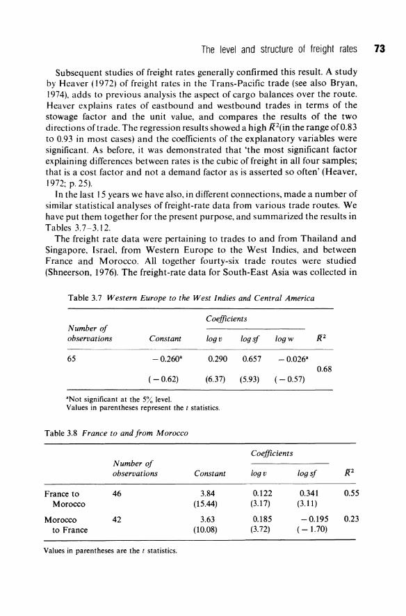
The level and structure of freight rates 73
Subsequent studies of freight rates generally confirmed this result. A study by Heaver (1972) of freight rates in the Trans-Pacific trade (see also Bryan, 1974), adds to previous analysis the aspect of cargo balances over the route. Heaver explains rates of eastbound and westbound trades in terms of the stowage factor and the unit value, and compares the results of the two directions of trade. The regression results showed a high jP(in the range of 0.83 to 0.93 in most cases) and the coefficients of the explanatory variables were significant. As before, it was demonstrated that 'the most significant factor explaining differences between rates is the cubic of freight in all four samples; that is a cost factor and not a demand factor as is asserted so often' (Heaver, 1972; p.25).
In the last 15 years we have also, in different connections, made a number of similar statistical analyses of freight-rate data from various trade routes. We have put them together for the present purpose, and summarized the results in Tables 3.7-3.12.
The freight rate data were pertaining to trades to and from Thailand and Singapore, Israel, from Western Europe to the West Indies, and between France and Morocco. All together fourty-six trade routes were studied (Shneerson, 1976). The freight-rate data for South-East Asia was collected in
Table 3.7 Western Europe to the West Indies and Central America
Coefficients Number of observations Constant log v
65 -0.260" 0.290
(- 0.62) (6.37)
aNot significant at the 5% level. Values in parentheses represent the t statistics.
Table 3.8 France to and from Morocco
France to Morocco
Morocco to France
Number of observations
46
42
Values in parentheses are the t statistics.
Constant
3.84 (15.44)
3.63 (10.08)
log sf logw R2
0.657 - 0.026" 0.68
(5.93) (- 0.57)
Coefficients
log v log sf
0.122 0.341 (3.17) (3.11)
0.l85 -0.195 (3.72) ( - 1.70)
R2
0.55
0.23
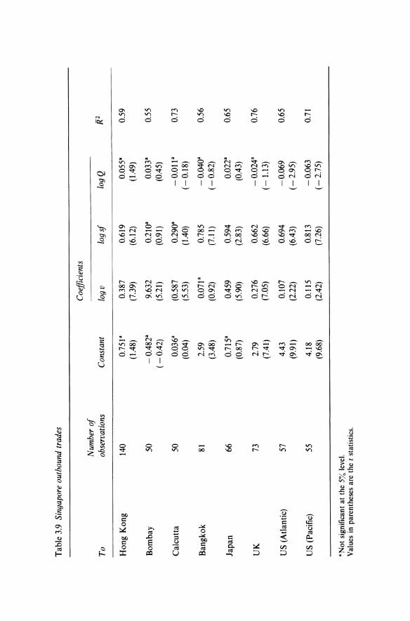
Tab
le 3
.9 S
inga
pore
out
boun
d tr
ades
Coe
ffici
ents
N
umbe
r o
f To
ob
serv
atio
ns
Con
stan
t lo
g v
log
sf
10gQ
R2
Hon
g K
ong
140
0.75
1a
0.38
7 0.
619
0.05
Y
0.59
(1
.48)
(7
.39)
(6
.12)
(1
.49)
Bom
bay
50
-0.
482a
9.
632
0.21
0'
0.03
3a
0.55
(-
0.42
) (5
.21)
(0
.91
) (0
.45)
Cal
cutt
a 50
0.
036a
(0
.587
0.
290a
-O
.Oll
a 0.
73
(0.0
4)
(5.5
3)
(1.4
0)
(-
0.18
)
Ban
gkok
81
2.
59
0.07
1a
0.78
5 -0
.040
a 0.
56
(3.4
8)
(0.9
2)
(7.1
1)
(-
0.82
)
Japa
n 66
0.
71Y
0.
459
0.59
4 O
.022
a 0.
65
(0.8
7)
(5.9
0)
(2.8
3)
(0.4
3)
UK
73
2.
79
0.27
6 0.
662
-0.0
24a
0.
76
(7.4
1)
(7.0
5)
(6.6
6)
(-
1.13
)
US
(Atl
anti
c)
57
4.43
0.
107
0.69
4 -0
.06
9
0.65
(9
.91)
(2
.22)
(6
.43)
(-
2.9
5)
US
(Pa
cifi
c)
55
4.18
0.
115
0.81
3 -0
.06
3
0.71
(9
.68)
(2
.42)
(7
.26)
(-
2.7
5)
a N
ot s
igni
fica
nt a
t th
e 5%
lev
el.
Val
ues
in p
aren
thes
es a
re t
he t
sta
tist
ics.
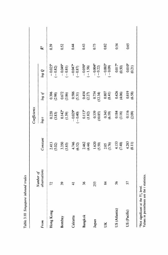
Tab
le 3
.10
Sing
apor
e in
boun
d tr
ades
Coe
ffici
ents
N
umbe
r o
f Fr
om
obse
rvat
ions
C
onst
ant
log
v lo
g sf
lo
g Q
f{2
Hon
g K
ong
72
2.41
3 0.
220
0.39
6 -
O.0
2Y
0.39
(5
.02)
(3
.83)
(2
.98)
(-
0.82
)
Bom
bay
39
3.35
0 0.
142-
0.67
2 -0
.04
9-
0.52
(3
.85)
(1
.59)
(3
.86)
(-
0.8
1)
Cal
cutt
a 41
4.
746
-0.0
29-
0.58
6 -0
.047
-0.
44
(6.5
2)
(-0.
40)
(5.3
1)
( -0.
87)
Ban
gkok
36
2.
462
0.11
3-0.
454
-0.0
50-
0.43
(4
.44)
(1
.82)
(2
.27)
(-
1.56
)
Japa
n 25
3 1.
620
0.33
9 0.
754
-0.0
04-
0.75
(5
.59)
(1
0.85
) (1
2.34
) ( -
0.22
)
UK
84
2.
05
0.34
3 0.
807
-0.0
03-
0.82
(3
.76)
(6
.19)
(8
.41
) (-
0.09
)
US
(Atla
ntic
) 56
4.
153
0.18
4 0.
426
0.01
7-0.
54
(7.4
8)
(3.1
6)
(4.0
6)
(0.5
0)
US
(Pac
ific)
57
4.
283
0.11
6 0.
819
0.01
0-0.
65
(8.1
1 )
(2.0
9)
(6.5
8)
(0.2
1 )
a N
ot s
igni
fica
nt a
t th
e 5%
lev
el.
Val
ues
in p
aren
thes
es a
re t
he t
sta
tist
ics.

Tab
le 3
.11
Thai
land
out
boun
d an
d in
boun
d tr
ades
Out
boun
d In
boun
d
Coe
ffici
ents
C
oeffi
cien
ts
Num
ber
of
Num
ber
of
To
andf
rom
ob
serv
atio
ns
Con
stan
t lo
g v
log
sf
iF
obse
rvat
ions
C
onst
ant
log
v lo
g sf
j{
2
Sing
apor
e 33
2.
399
0.04
28
0.45
1 0.
29
36
2.79
1 0.
178
0.39
1 0.
10
(0.9
94)
(3.2
28)
(2.3
18)
(2.7
77)
Hon
g K
ong
44
2.57
9 0.
185
0.22
7 0.
26
101
2.22
3 0.
330
0.23
38
0.27
(3
.09)
(1
.684
(4
.246
) (1
.23)
Cal
cutt
a 9
2.15
7 0.
1698
0.
552
0.78
63
2.
559
0.15
6 0.
562
0.35
(1
.75)
(2
.083
) (2
.914
) (4
.581
)
Japa
n 35
2.
589
0.16
78
0.56
5 0.
30
129
2.85
6 0.
238
0.25
5 0.
34
(1.7
62)
(2.4
65)
(5.3
04)
(2.5
74)
Bom
bay
8 2.
422
0.12
7"
-0.0
06"
0.30
55
2.
524
0.19
7 0.
361
0.61
(2
.172
) (-
0.02
9)
(3.6
57)
(3.7
16)
UK
21
2.
639
0.17
0 0.
372
0.74
10
9 3.
042
0.14
7 0.
398
0.52
(2
.956
) (3
.586
) (4
.919
) (5
.884
)
US
(Pac
ific
) 13
1.
727
0.64
5 0.
625
0.31
10
8 2.
326
0.28
2 0.
3468
0.
25
(2.3
35)
(1.2
67)
(5.2
87)
(1.8
5)
US
(Atla
ntic
) 9
6.05
0.
182
0.84
5 0.
97
109
2.24
5 0.
498
-0.2
07"
0.33
(8
.31)
(7
.0)
(1.1
81)
(-
0.72
)
aNot
sig
nifi
cant
at
the
5% le
vel.
Val
ues
in p
aren
thes
es a
re t
he t
sta
tistic
s.
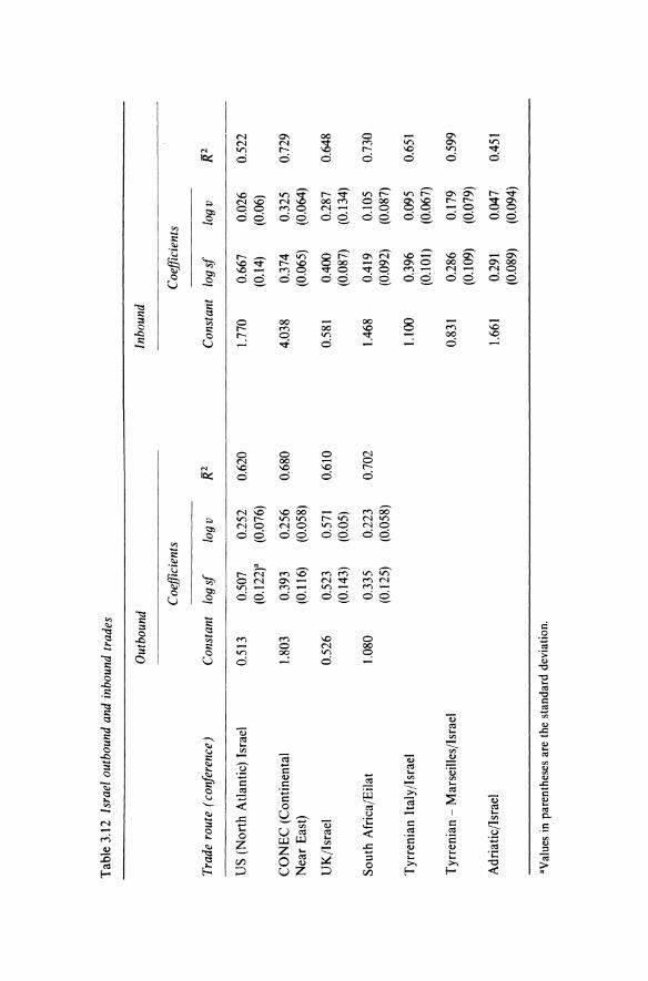
Tab
le 3
.12
Isra
el o
utbo
und
and
inbo
und
trad
es
Out
boun
d In
boun
d
Coe
ffici
ents
C
oeffi
cien
ts
Trad
e ro
ute
(con
fere
nce)
C
onst
ant
log
sf
log
v iF
C
onst
ant
log
sf
log
v IF
US
(Nor
th A
tlant
ic)
Isra
el
0.51
3 0.
507
0.25
2 0.
620
1.77
0 0.
667
0.02
6 0.
522
(0.1
22)"
(0
.076
) (0
.14)
(0
.06)
CO
NE
C (
Con
tinen
tal
1.80
3 0.
393
0.25
6 0.
680
4.03
8 0.
374
0.32
5 0.
729
Nea
r E
ast)
(0
.116
) (0
.058
) (0
.065
) (0
.064
)
UK
/Isr
ael
0.52
6 0.
523
0.57
1 0.
610
0.58
1 0.
400
0.28
7 0.
648
(0.1
43)
(0.0
5)
(0.0
87)
(0.1
34)
Sout
h A
fric
a/E
ilat
1.08
0 0.
335
0.22
3 0.
702
1.46
8 0.
419
0.10
5 0.
730
(0.1
25)
(0.0
58)
(0.0
92)
(0.0
87)
Tyr
reni
an I
taly
/Isr
ael
1.10
0 0.
396
0.09
5 0.
651
(0.1
01)
(0.0
67)
Tyr
reni
an -
Mar
seill
es/I
srae
l 0.
831
0.28
6 0.
179
0.59
9 (0
.109
) (0
.079
)
Adr
iatic
/Isr
ael
1.66
1 0.
291
0.04
7 0.
451
(0.0
89)
(0.0
94)
'Val
ues
in p
aren
thes
es a
re t
he s
tand
ard
devi
atio
n.
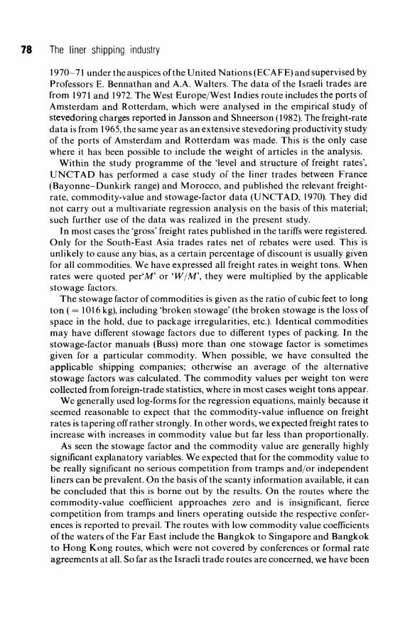
78 The liner shipping industry
1970-71 under the auspices of the United Nations (ECAFE) and supervised by Professors E. Bennathan and A.A. Walters. The data of the Israeli trades are from 1971 and 1972. The West Europe/West Indies route includes the ports of Amsterdam and Rotterdam, which were analysed in the empirical study of stevedoring charges reported in Jansson and Shneerson (1982). The freight-rate data is from 1965, the same year as an extensive stevedoring productivity study of the ports of Amsterdam and Rotterdam was made. This is the only case where it has been possible to include the weight of articles in the analysis.
Within the study programme of the 'level and structure of freight rates', UNCT AD has performed a case study of the liner trades between France (Bayonne-Dunkirk range) and Morocco, and published the relevant freightrate, commodity-value and stowage-factor data (UNCT AD, 1970). They did not carry out a multivariate regression analysis on the basis of this material; such further use of the data was realized in the present study.
In most cases the 'gross' freight rates published in the tariffs were registered. Only for the South-East Asia trades rates net of rebates were used. This is unlikely to cause any bias, as a certain percentage of discount is usually given for all commodities. We have expressed all freight rates in weight tons. When rates were quoted per'M' or 'W/M', they were multiplied by the applicable stowage factors.
The stowage factor of commodities is given as the ratio of cubic feet to long ton ( = 1016 kg), including 'broken stowage' (the broken stowage is the loss of space in the hold, due to package irregularities, etc.). Identical commodities may have different stowage factors due to different types of packing. In the stowage-factor manuals (Buss) more than one stowage factor is sometimes given for a particular commodity. When possible, we have consulted the applicable shipping companies; otherwise an average of the alternative stowage factors was calculated. The commodity values per weight ton were collected from foreign-trade statistics, where in most cases weight tons appear.
We generally used log-forms for the regression equations, mainly because it seemed reasonable to expect that the commodity-value influence on freight rates is tapering off rather strongly. In other words, we expected freight rates to increase with increases in commodity value but far less than proportionally.
As seen the stowage factor and the commodity value are generally highly significant explanatory variables. We expected that for the commodity value to be really significant no serious competition from tramps and/or independent liners can be prevalent. On the basis of the scanty information available, it can be concluded that this is borne out by the results. On the routes where the commodity-value coeffiicient approaches zero and is insignificant, fierce competition from tramps and liners operating outside the respective conferences is reported to prevail. The routes with low commodity value coefficients of the waters of the Far East include the Bangkok to Singapore and Bangkok to Hong Kong routes, which were not covered by conferences or formal rate agreements at all. So far as the Israeli trade routes are concerned, we have been
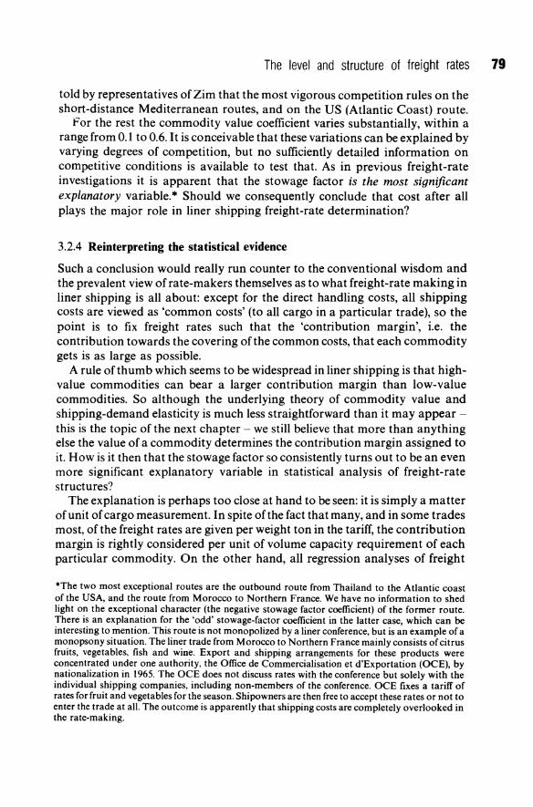
The level and structure of freight rates 79
told by representatives of Zim that the most vigorous competition rules on the short-distance Mediterranean routes, and on the US (Atlantic Coast) route.
for the rest the commodity value coefficient varies substantially, within a range from 0.1 to 0.6. I t is conceivable that these variations can be explained by varying degrees of competition, but no sufficiently detailed information on competitive conditions is available to test that. As in previous freight-rate investigations it is apparent that the stowage factor is the most significant explanatory variable.* Should we consequently conclude that cost after all plays the major role in liner shipping freight-rate determination?
3.2.4 Reinterpreting the statistical evidence
Such a conclusion would really run counter to the conventional wisdom and the prevalent view of rate-makers themselves as to what freight-rate making in liner shipping is all about: except for the direct handling costs, all shipping costs are viewed as 'common costs' (to all cargo in a particular trade), so the point is to fix freight rates such that the 'contribution margin', i.e. the contribution towards the covering of the common costs, that each commodity gets is as large as possible.
A rule of thumb which seems to be widespread in liner shipping is that highvalue commodities can bear a larger contribution margin than low-value commodities. So although the underlying theory of commodity value and shipping-demand elasticity is much less straightforward than it may appear -this is the topic of the next chapter - we still believe that more than anything else the value of a commodity determines the contribution margin assigned to it. How is it then that the stowage factor so consistently turns out to be an even more significant explanatory variable in statistical analysis of freight-rate structures?
The explanation is perhaps too close at hand to be seen: it is simply a matter of unit of cargo measurement. In spite ofthe fact that many, and in some trades most, of the freight rates are given per weight ton in the tariff, the contribution margin is rightly considered per unit of volume capacity requirement of each particular commodity. On the other hand, all regression analyses of freight
*The two most exceptional routes are the outbound route from Thailand to the Atlantic coast of the USA, and the route from Morocco to Northern France. We have no information to shed light on the exceptional character (the negative stowage factor coefficient) of the former route. There is an explanation for the 'odd' stowage-factor coefficient in the latter case, which can be interesting to mention. This route is not monopolized by a liner conference, but is an example of a monopsony situation. The liner trade from Morocco to Northern France mainly consists of citrus fruits, vegetables, fish and wine. Export and shipping arrangements for these products were concentrated under one authority, the Office de Commercialisation et d'Exportation (OCE), by nationalization in 1965. The OCE does not discuss rates with the conference but solely with the individual shipping companies, including non-members of the conference. OCE fixes a tarilT of rates for fruit and vegetables for the season. Shipowners are then free to accept these rates or not to enter the trade at all. The outcome is apparently that shipping costs are completely overlooked in the rate-making.
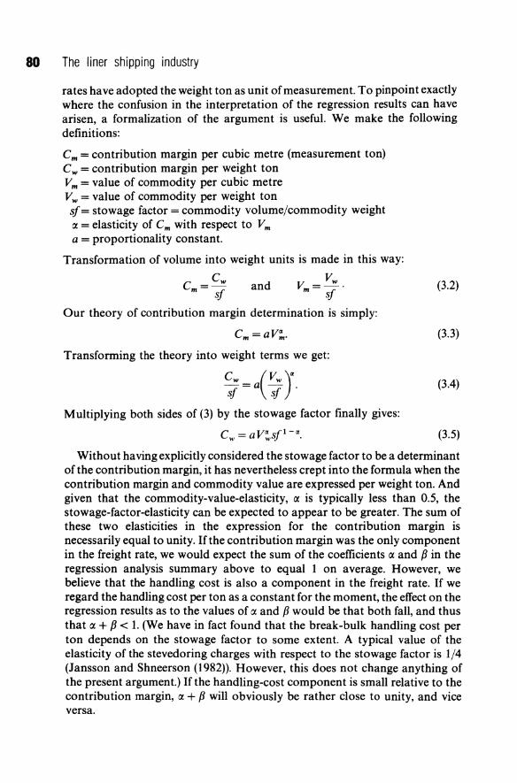
80 The liner shipping industry
rates have adopted the weight ton as unit of measurement. To pinpoint exactly where the confusion in the interpretation of the regression results can have arisen, a formalization of the argument is useful. We make the following definitions:
Cm = contribution margin per cubic metre (measurement ton) Cw = contribution margin per weight ton Vm = value of commodity per cubic metre Vw = value of commodity per weight ton sf = stowage factor = commodity volume/commodity weight oc = elasticity of Cm with respect to Vm a = proportionality constant.
Transformation of volume into weight units is made in this way:
C = Cw m sf and
Vw V =-. m sf
Our theory of contribution margin determination is simply:
Cm=aV~.
Transforming the theory into weight terms we get:
~j=a(:j r Multiplying both sides of (3) by the stowage factor finally gives:
Cw = aV~sfl-a.
(3.2)
(3.3)
(3.4)
(3.5)
Without having explicitly considered the stowage factor to be a determinant ofthe contribution margin, it has nevertheless crept into the formula when the contribution margin and commodity value are expressed per weight ton. And given that the commodity-value-elasticity, oc is typically less than 0.5, the stowage-factor-elasticity can be expected to appear to be greater. The sum of these two elasticities in the expression for the contribution margin is necessarily equal to unity. If the contribution margin was the only component in the freight rate, we would expect the sum of the coefficients oc and f3 in the regression analysis summary above to equal 1 on average. However, we believe that the handling cost is also a component in the freight rate. If we regard the handling cost per ton as a constant for the moment, the effect on the regression results as to the values of oc and f3 would be that both fall, and thus that oc + f3 < 1. (We have in fact found that the break-bulk handling cost per ton depends on the stowage factor to some extent. A typical value of the elasticity of the stevedoring charges with respect to the stowage factor is 1/4 (Jansson and Shneerson (1982)). However, this does not change anything of the present argument.) If the handling-cost component is small relative to the contribution margin, oc + f3 will obviously be rather close to unity, and vice versa.
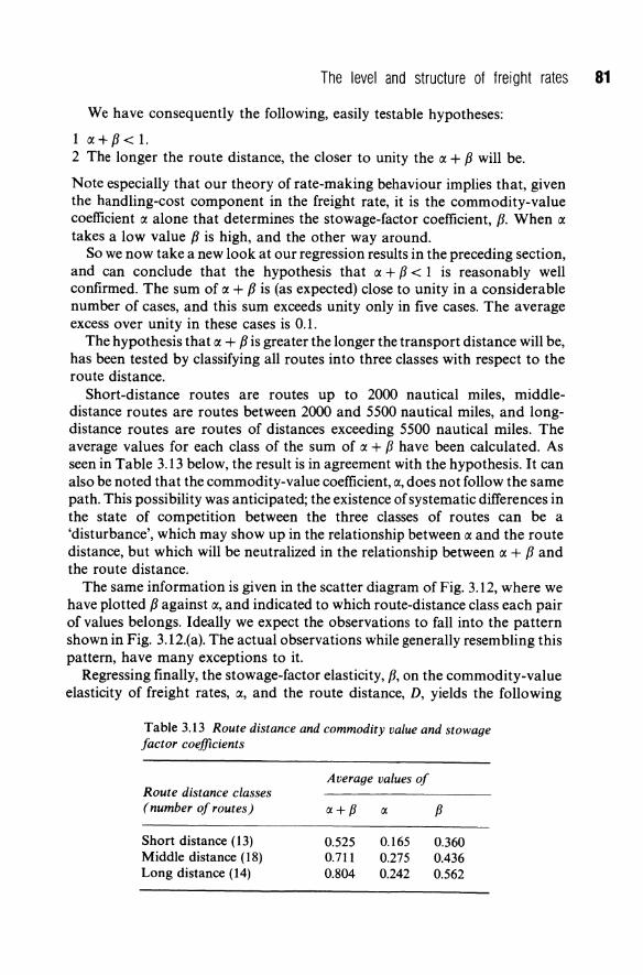
The level and structure of freight rates 81
We have consequently the following, easily testable hypotheses:
1 rx+f3<I. 2 The longer the route distance, the closer to unity the rx + f3 will be.
Note especially that our theory of rate-making behaviour implies that, given the handling-cost component in the freight rate, it is the commodity-value coefficient rx alone that determines the stowage-factor coefficient, f3. When rx takes a low value f3 is high, and the other way around.
So we now take a new look at our regression results in the preceding section, and can conclude that the hypothesis that rx + f3 < 1 is reasonably well confirmed. The sum of rx + f3 is (as expected) close to unity in a considerable number of cases, and this sum exceeds unity only in five cases. The average excess over unity in these cases is O.I.
The hypothesis that rx + f3 is greater the longer the transport distance will be, has been tested by classifying all routes into three classes with respect to the route distance.
Short-distance routes are routes up to 2000 nautical miles, middledistance routes are routes between 2000 and 5500 nautical miles, and longdistance routes are routes of distances exceeding 5500 nautical miles. The average values for each class of the sum of rx + f3 have been calculated. As seen in Table 3.13 below, the result is in agreement with the hypothesis. It can also be noted that the commodity-value coefficient, rx, does not follow the same path. This possibility was anticipated; the existence of systematic differences in the state of competition between the three classes of routes can be a 'disturbance', which may show up in the relationship between rx and the route distance, but which will be neutralized in the relationship between rx + f3 and the route distance.
The same information is given in the scatter diagram of Fig. 3.12, where we have plotted f3 against rx, and indicated to which route-distance class each pair of values belongs. Ideally we expect the observations to fall into the pattern shown in Fig. 3.12.(a). The actual observations while generally resembling this pattern, have many exceptions to it.
Regressing finally, the stowage-factor elasticity, f3, on the commodity-value elasticity of freight rates, rx, and the route distance, D, yields the following
Table 3.13 Route distance and commodity value and stowage factor coefficients
Average values of Route distance classes (number of routes) ex+{3 ex {3
Short distance (13) 0.525 0.165 0.360 Middle distance (18) 0.711 0.275 0.436 Long distance (14) 0.804 0.242 0.562
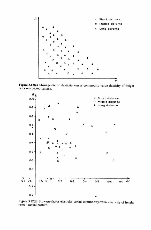
~
• • • • • • • 0 0
0 • 0
0 • 0
)( 0 0 )(
)( 0
0 X
X X
)( X
)( X
)( X
" " " " 0 • 0
0 0 0
)(
X X
" " • 0
0
• "
x Short distance
o Middle distance
A- Long distance
• A-
• 0(
Figure 3.12(a) Stowage-factor elasticity versus commodity-value elasticity of freight rates - expected pattern.
(3
o·g
0·8
0·7
0·6 x
0·5
0·4
0·3
0·2
0·1
().1 0·5
0·1
0·2
.. )(
" 0
)( x
R x
)(
0·5 0'1
•
0
~
" " x x
" 0 0
0 0
x x
I
0·2
x Short distance 0 Middle distance A- Long distance •
0
• x " 0
0 0
0 0
" 0
x
x 0
0·3 0·4 0·5 0·6 0·7 0{
Figure 3.11(b) Stowage-factor elasticity versus commodity-value elasticity of freight rates - actual pattern.
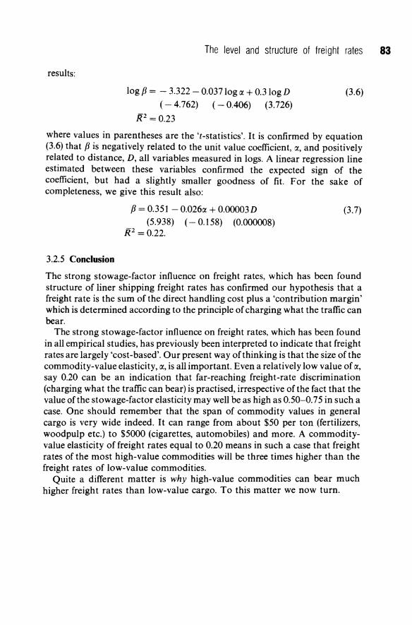
The level and structure of freight rates 83
results:
log fJ = - 3.322 - 0.037 log (I. + 0.3 log D (3.6) ( - 4.762) ( - 0.406) (3.726)
IP =0.23
where values in parentheses are the 't-statistics'. It is confirmed by equation (3.6) that fJ is negatively related to the unit value coefficient, (I., and positively related to distance, D, all variables measured in logs. A linear regression line estimated between these variables confirmed the expected sign of the coefficient, but had a slightly smaller goodness of fit. For the sake of completeness, we give this result also:
3.2.5 Conclusion
fJ = 0.351 - 0.026(1. + 0.00003D
(5.938) (- 0.158) (0.000008) IP = 0.22.
(3.7)
The strong stowage-factor influence on freight rates, which has been found structure of liner shipping freight rates has confirmed our hypothesis that a freight rate is the sum of the direct handling cost plus a 'contribution margin' which is determined according to the principle of charging what the traffic can bear.
The strong stowage-factor influence on freight rates, which has been found in all empirical studies, has previously been interpreted to indicate that freight rates are largely 'cost-based'. Our present way of thinking is that the size of the commodity-value elasticity, (I., is all important. Even a relatively low value of (I., say 0.20 can be an indication that far-reaching freight-rate discrimination (charging what the traffic can bear) is practised, irrespective of the fact that the value of the stowage-factor elasticity may well be as high as 0.50-0.75 in such a case. One should remember that the span of commodity values in general cargo is very wide indeed. It can range from about $50 per ton (fertilizers, woodpulp etc.) to $5000 (cigarettes, automobiles) and more. A commodityvalue elasticity of freight rates equal to 0.20 means in such a case that freight rates of the most high-value commodities will be three times higher than the freight rates of low-value commodities.
Quite a different matter is why high-value commodities can bear much higher freight rates than low-value cargo. To this matter we now turn.
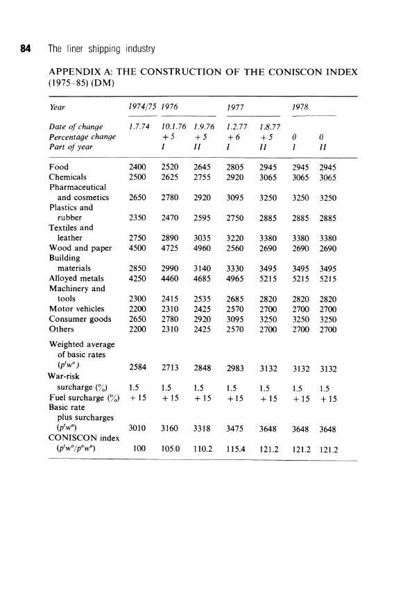
84 The liner shipping industry
APPENDIX A: THE CONSTRUCTION OF THE CONISCON INDEX (1975-85) (DM)
Year 1974/75 1976 1977 1978 ----
Date of change 1.7.74 10.1.76 1.9.76 1.2.77 1.8.77 Percentage change +5 +5 +6 +5 a a Part of year I II I II I II
Food 2400 2520 2645 2805 2945 2945 2945 Chemicals 2500 2625 2755 2920 3065 3065 3065 Pharmaceutical
and cosmetics 2650 2780 2920 3095 3250 3250 3250 Plastics and
rubber 2350 2470 2595 2750 2885 2885 2885 Textiles and
leather 2750 2890 3035 3220 3380 3380 3380 Wood and paper 4500 4725 4960 2560 2690 2690 2690 Building
materials 2850 2990 3140 3330 3495 3495 3495 Alloyed metals 4250 4460 4685 4965 5215 5215 5215 Machinery and
tools 2300 2415 2535 2685 2820 2820 2820 Motor vehicles 2200 2310 2425 2570 2700 2700 2700 Consumer goods 2650 2780 2920 3095 3250 3250 3250 Others 2200 2310 2425 2570 2700 2700 2700
Weighted average of basic rates (p'WO ) 2584 2713 2848 2983 3132 3132 3132
War-risk surcharge (%) 1.5 1.5 1.5 1.5 1.5 1.5 1.5
Fuel surcharge (%) + 15 + 15 + 15 + 15 + 15 + 15 + 15 Basic rate
plus surcharges (p'WO) 3010 3160 3318 3475 3648 3648 3648
CONISCON index (p'WO / pOWO) 100 105.0 110.2 115.4 121.2 121.2 121.2
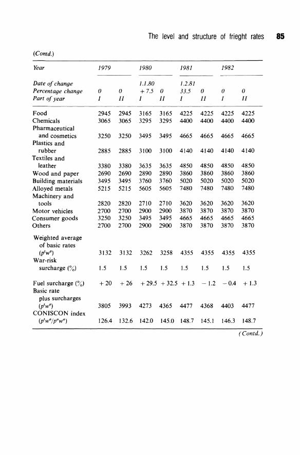
The level and structure of frieght rates 85
(Contd.)
Year 1979 1980 1981 1982
Date of change 1.1.80 1.2.81 Percentage change 0 0 + 7.5 0 33.5 0 0 0 Part of year I II I II I II I II
Food 2945 2945 3165 3165 4225 4225 4225 4225 Chemicals 3065 3065 3295 3295 4400 4400 4400 4400 Pharmaceutical
and cosmetics 3250 3250 3495 3495 4665 4665 4665 4665 Plastics and
rubber 2885 2885 3100 3100 4140 4140 4140 4140 Textiles and
leather 3380 3380 3635 3635 4850 4850 4850 4850 Wood and paper 2690 2690 2890 2890 3860 3860 3860 3860 Building materials 3495 3495 3760 3760 5020 5020 5020 5020 Alloyed metals 5215 5215 5605 5605 7480 7480 7480 7480 Machinery and
tools 2820 2820 2710 2710 3620 3620 3620 3620 Motor vehicles 2700 2700 2900 2900 3870 3870 3870 3870 Consumer goods 3250 3250 3495 3495 4665 4665 4665 4665 Others 2700 2700 2900 2900 3870 3870 3870 3870
Weighted average of basic rates (p'WO ) 3132 3132 3262 3258 4355 4355 4355 4355
War-risk surcharge (%) 1.5 1.5 1.5 1.5 1.5 1.5 1.5 1.5
Fuel surcharge (%) +20 + 26 + 29.5 + 32.5 + 1.3 -1.2 -0.4 +1.3 Basic rate
plus surcharges (p'WO ) 3805 3993 4273 4365 4477 4368 4403 4477
CONISCON index (p'wo/poWO ) 126.4 132.6 142.0 145.0 148.7 145.1 146.3 148.7
(Contd.)
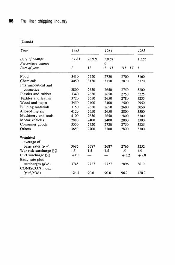
86 The liner shipping industry
(Contd.)
Year 1983 1984 1985
Date of change 1.1.83 26.9.83 7.8.84 1.2.85 Percentage change 0 Part of year I II I II III IV I
Food 3410 2720 2720 2700 3160 Chemicals 4050 3150 3150 2870 3370 Pharmaceutical and
cosmetics 3800 2650 2650 2750 3200 Plastics and rubber 3340 2650 2650 2750 3225 Textiles and leather 3720 2650 2650 2780 3235 Wood and paper 3450 2400 2400 2500 2950 Building materials 3150 2650 2650 2600 3050 Alloyed metals 4120 2650 2650 2800 3300 Machinery and tools 4100 2650 2650 2800 3300 Motor vehicles 2880 2400 2400 2800 3300 Consumer goods 3550 2720 2720 2750 3225 Others 3650 2700 2700 2800 3300
Weighted average of basic rates (p'WO) 3686 2687 2687 2766 3252
War-risk surcharge (%) 1.5 1.5 1.5 1.5 1.5 Fuel surcharge (%) +O.l +3.2 +9.8 Basic rate plus
surcharges (p'WO) 3745 2727 2727 2896 3619 CONISCON index
(p'wo/poWO) 124.4 90.6 90.6 96.2 120.2
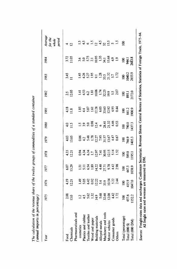
The
calc
ulat
ion
of t
he r
even
ue s
hare
of t
he t
wel
ve g
roup
s o
f com
mod
ities
of a
sta
ndar
d co
ntai
ner
(ann
ual
impo
rts
in p
erce
ntag
e)
Year
19
75
1976
19
77
1978
19
79
1980
19
81
1982
19
83
1984
Av
erag
e fo
r th
e w
hole
pe
riod
Foo
d 2.
88
4.19
6.
07
4.33
4.
03
4.0
4.18
2.
5 3.
45
3.72
4
Che
mic
als
13.0
12
.21
13.2
9 12
.21
13.0
5 11
.5
11.8
12
.05
11
11.0
5 12
P
harm
aceu
tica
ls a
nd
cosm
etic
s 1.
2 1.
49
1.51
0.
94
0.86
1.
5 1.
85
1.41
1.
45
3.6
1.5
Pla
stic
s an
d ru
bber
4.
5 5.
05
5.11
4.
34
4.2
3.9
4.4
4.53
4.
26
5.0
4.5
Tex
tiles
and
lea
ther
5.
62
6.42
6.
54
6.34
5.
48
5.0
5.87
6.
2 5.
27
5.75
6
Woo
d an
d pa
per
1.32
0.
92
1.89
1.
7 1.
78
0.98
1.
61
1.81
1.
95
2.1
1.5
Bui
ldin
g m
ater
ials
14
.9
12.2
2 14
.22
12.9
7 12
.27
12.4
12
.28
10.0
6 9.
1 10
.95
12
Allo
yed
met
als
5.68
5.
4 4.
48
7.41
7.
95
6 6.
05
1.74
1.
28
1.35
4.
5 M
achi
nery
and
too
ls
32.6
8 33
.9
27.7
1 30
.95
31.5
7 28
.41
33.6
5 32
.23
33.5
34
.1
32
Mot
or v
ehic
les
12.0
8 10
.54
9.78
12
.15
13.6
7 21
.32
12.9
2 19
.9
21.3
2 15
.68
15.5
C
onsu
mer
goo
ds
4.42
5.
22
4.42
5.
14
4.47
4.
46
4.95
5.
5 5.
7 4.
9 5
Oth
ers
1.72
2.
44
2.98
1.
52
0.67
0.
53
0.44
2.
07
1.72
1.
9 1.
5
Tot
al (
perc
enta
ge)
100
100
100
100
100
100
100
100
100
100
100
Tot
al (
000
$)
457.
6 41
5.9
447.
5 58
9.8
766.
9 79
0.0
841.
2 89
5.1
1040
.2
944.
1 T
otal
(00
0 O
M)
1152
.2
1047
.0
1038
.9
1195
.1
1405
.3
1437
.3
1900
.9
2172
.0
2655
.9
26g3
.8
Sour
ces:
Fre
ight
-rat
es d
ata
and
surc
harg
es:
Con
fere
nce
Sec
reta
riat
. R
even
ue S
hare
s: C
entr
al B
urea
u of
Sta
tist
ics,
Sta
tist
ics
of F
orei
gn T
rade
, 19
75-8
4.
All
frei
ght
rate
s an
d re
venu
es a
re m
easu
red
in O
M.
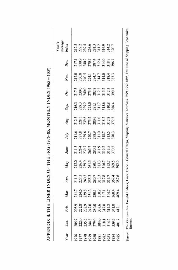
AP
PE
ND
IX B
: T
HE
LIN
ER
IN
DE
X O
F T
HE
FR
G (
1976
-85,
MO
NT
HL
Y I
ND
EX
196
5 =
10
03)
Year
ly
aver
age
Year
Ja
n.
Feb.
M
ar.
Apr
. M
ay
June
Ju
ly
Aug
. Se
p.
Oct
. N
ov.
Dec
. in
dex
1976
20
5.9
205.
9 21
1.7
211.
5 21
2.0
211.
5 21
1.6
212.
5 21
6.3
217.
5 21
7.0
217.
1 21
2.5
1977
22
2.0
222.
8·
224.
6 22
7.3
226.
4 22
6.4
227.
8 22
8.5
229.
3 23
0.0
230.
8 23
0.9
227.
2 19
78
235.
5 23
8.9
239.
8 24
0.3
239.
9 23
9.7
239.
6 23
9.6
239.
2 24
0.0
240.
5 24
0.2
239.
4 19
79
244.
8 24
7.0
251.
3 25
5.3
261.
5 26
5.7
270.
7 27
3.2
275.
0 27
3.4
274.
1 27
0.7
263.
6 19
80
279.
0 28
0.0
280.
3 28
0.7
280.
4 28
0.2
278.
9 28
0.6
281.
1 28
2.8
284.
7 28
7.4
281.
3 19
81
304.
0 30
7.6
310.
9 31
3.3
313.
3 31
1.9
311.
0 31
1.0
311.
7 31
2.2
314.
7 31
2.4
311.
2 19
82
318.
1 31
7.0
317.
1 31
7.8
316.
7 31
9.2
318.
7 31
8.2
315.
6 31
5.2
314.
0 31
4.0
316.
9 19
83
314.
2 31
4.2
314.
7 31
3.7
313.
7 31
3.5
313.
5 31
2.8
310.
8 31
2.3
318.
4 31
8.7
314.
2 19
84
339.
6 34
1.0
360.
4 36
7.4
369.
5 37
0.5
370.
3 37
2.5
386.
4 39
0.7
383.
3 39
6.7
370.
7 19
85
401.
7 41
2.1
409.
4 38
7.6
392.
9
Sour
ce:
The
Ger
man
Sea
Fre
ight
Ind
ices
; L
iner
Tra
de -
Gen
eral
Car
go,
Ship
ping
Sta
tistic
s Ye
arbo
ok 1
979,
19.2
, 189
5, I
nsti
tute
of
Shi
ppin
g E
cono
mic
s,
Bre
men
.

The level and structure of freight rates 89
APPENDIX C: THE CONSTRUCTION OF AN INDIVIDUAL LINE FREIGHT RATE INDEX (QUARTERLY DATA FOR THE PERIOD 1976-85 IN DM AND $)
Revenue data on the Hamburg-Israel trade route (quarterly datafor the period 1976-85 in DM) Revenue first quarter (January-March)
Quantities Average per TEU
Total Weight Weight Year revenue TEUs (tons) Revenue (tons)
1976 468550 285 3595 1614 12.6 1977 586200 292 3533 2008 12.1 1978 321750 195 1755 1650 9.0 1979 417350 357 3945 1169 11.0 1980 405400 326 3227 1244 9.9 1981 689200 539 6040 1279 11.2 1982 661850 409 3967 1618 9.7 1983 684200 412 4162 1661 10.1 1984 458144 399 4271 1148 10.7 1985 1039600 631 7669 1648 12.1
Revenue second quarter (April-June)
Quantities Average per TEU
Total Weight Weight Year revenue TEUs (tons) Revenue (tons)
1976 414000 294 2442 1407 8.3 1977 301250 177 1620 1702 9.1 1978 417150 310 3690 1346 11.9 1979 454700 392 4563 1160 11.6 1980 293600 270 2808 1087 10.4 1981 478950 362 4163 1323 11.5 1982 529950 334 3730 1587 11.2 1983 692400 492 4564 1407 9.3 1984 585000 595 6959 983 11.7 1985 1392450 772 9600 1803.5 12.4
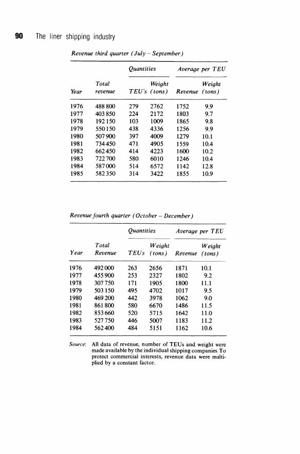
90 The liner shipping industry
Revenue third quarter (July - September)
Quantities Average per TEV
Total Weight Weight Year revenue TEV's (tons) Revenue (tons)
1976 488800 279 2762 1752 9.9 1977 403850 224 2172 1803 9.7 1978 192150 103 1009 1865 9.8 1979 550150 438 4336 1256 9.9 1980 507900 397 4009 1279 10.1 1981 734450 471 4905 1559 10.4 1982 662450 414 4223 1600 10.2 1983 722700 580 6010 1246 10.4 1984 587000 514 6572 1142 12.8 1985 582350 314 3422 1855 10.9
Revenue fourth quarter (October - December)
Quantities Average per TEV
Total Weight Weight Year Revenue TEVs (tons) Revenue (tons)
1976 492000 263 2656 1871 10.1 1977 455900 253 2327 1802 9.2 1978 307750 171 1905 1800 11.1 1979 503150 495 4702 1017 9.5 1980 469200 442 3978 1062 9.0 1981 861800 580 6670 1486 11.5 1982 853660 520 5715 1642 11.0 1983 527750 446 5007 1183 11.2 1984 562400 484 5151 1162 10.6
Source: All data of revenue, number of TEUs and weight were made available by the individual shipping companies, To protect commercial interests, revenue data were multi-plied by a constant factor.
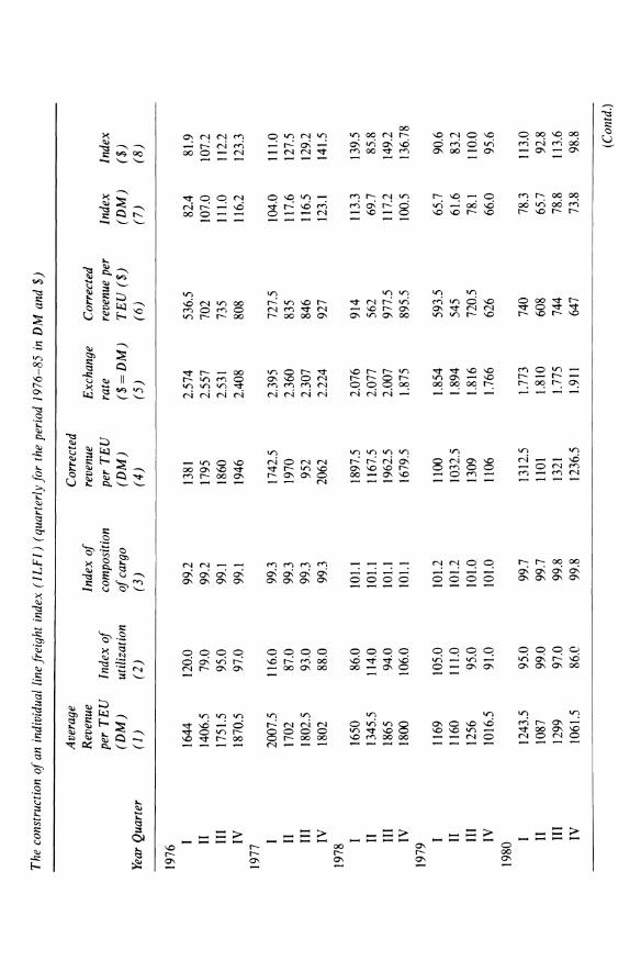
The
cons
truc
tion
of a
n in
divi
dual
lin
e fr
eigh
t in
dex
(I L
F I)
(qu
arte
rly
for
the
peri
od 1
976-
85 i
n D
M a
nd $
)
Ave
rage
C
orre
cted
R
even
ue
Inde
x o
f re
venu
e E
xcha
nge
Cor
rect
ed
per
TE
U
Inde
x o
f co
mpo
sitio
n pe
r T
EU
ra
te
reve
nue
per
Inde
x In
dex
(DM
) ut
iliza
tion
of c
argo
(D
M)
($=
DM
) T
EU
($
) (D
M)
($)
Year
Qua
rter
(1
) (2
) (3
) (4
) (5
) (6
) (7
) (8
)
1976
I 16
44
120.
0 99
.2
1381
2.
574
536.
5 82
.4
81.9
II
14
06.5
79
.0
99.2
17
95
2.55
7 70
2 10
7.0
107.
2 II
I 17
51.5
95
.0
99.1
18
60
2.53
1 73
5 11
1.0
112.
2 IV
18
70.5
97
.0
99.1
19
46
2.40
8 80
8 11
6.2
123.
3 19
77
2007
.5
116.
0 99
.3
1742
.5
2.39
5 72
7.5
104.
0 11
1.0
II
1702
87
.0
99.3
19
70
2.36
0 83
5 11
7.6
127.
5 II
I 18
02.5
93
.0
99.3
95
2 2.
307
846
116.
5 12
9.2
IV
1802
88
.0
99.3
20
62
2.22
4 92
7 12
3.1
141.
5 19
78 I
1650
86
.0
101.
1 18
97.5
2.
076
914
113.
3 13
9.5
II
1345
.5
114.
0 10
1.1
1167
.5
2.07
7 56
2 69
.7
85.8
II
I 18
65
94.0
10
1.1
1962
.5
2.00
7 97
7.5
117.
2 14
9.2
IV
1800
10
6.0
101.
1 16
79.5
1.
875
895.
5 10
0.5
136.
78
1979
I 11
69
105.
0 10
1.2
1100
1.
854
593.
5 65
.7
90.6
II
11
60
111.
0 10
1.2
1032
.5
1.89
4 54
5 61
.6
83.2
II
I 12
56
95.0
10
1.0
1309
1.
816
720.
5 78
.1
110.
0 IV
10
16.5
91
.0
101.
0 11
06
1.76
6 62
6 66
.0
95.6
19
80 I
1243
.5
95.0
99
.7
1312
.5
1.77
3 74
0 78
.3
113.
0 II
10
87
99.0
99
.7
1101
1.
810
608
65.7
92
.8
III
1299
97
.0
99.8
13
21
1.77
5 74
4 78
.8
113.
6 IV
10
61.5
86
.0
99.8
12
36.5
1.
911
647
73.8
98
.8
(Con
td.)
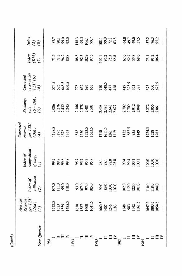
(Con
td.)
Ave
rage
C
orre
cted
R
even
ue
Inde
x o
f re
venu
e E
xcha
nge
Cor
rect
ed
per
TE
U
Inde
x o
f co
mpo
sitio
n pe
r T
EU
ra
te
reve
nue
per
Inde
x In
dex
(DM
) ut
iliza
tion
of c
argo
(D
M)
($=
DM
) T
EU
($
) (D
M)
($)
Year
Qua
rter
(1
) (2
) (3
) (4
) (5
) (6
) (7
) (8
)
1981
I 12
78.5
10
7.0
99.7
11
98.5
2.
086
574.
5 71
.5
87.7
II
13
23
111.
0 99
.7
1195
2.
276
525
71.3
80
.1
III
1559
99
.0
99.8
15
78
2.43
2 64
8.5
94.2
99
.0
IV
1485
.5
110.
0 99
.8
1353
2.
245
602.
5 80
.8
92.0
19
82 I
1618
93
.0
95.7
18
18
2.34
6 77
5 10
8.5
118.
3 II
15
87
107.
0 95
.7
1550
2.
378
652
92.5
99
.5
III
1600
97
.0
95.7
17
23.5
2.
481
695
102.
9 10
6.1
IV
1641
.5
105.
0 95
.7
1633
.5
2.50
1 65
3 97
.5
99.7
19
83 I
1660
.5
99.0
98
.1
1710
2.
408
710
102.
1 10
8.4
II
1407
89
.0
98.1
16
11.5
2.
485
648.
5 96
.2
99.0
II
I 12
46
100.
0 98
.8
1261
2.
643
477
75.3
72
.8
IV
1183
10
7.0
98.8
11
19
2.67
7 41
8 66
.8
63.8
19
84 I
1148
10
2.0
99.4
11
32
2.70
2 41
9 67
.6
64.0
II
98
3 11
2.0
99.4
88
2.5
2.70
9 32
5.5
52.7
49
.7
III
1142
12
2.0
100.
1 93
5 2.
912
321
55.8
49
.0
IV
1161
.5
101.
0 10
0.1
1149
3.
048
377
68.6
57
.5
1985
I 16
47.5
11
6.0
100.
0 12
24.5
3.
272
375
73.1
57
.2
II
1803
.5
118.
0 10
0.0
1528
3.
056
500
91.2
76
.3
III
1854
.5
104.
0 10
0.0
1783
2.
86
623.
5 10
6.4
95.2
IV

Exp
lana
tion
of c
onst
ruct
ion
of IL
FI i
s as
fol
low
s:
Col
umn
1 Fi
gure
obt
aine
d by
div
idin
g to
tal
reve
nue
by t
he n
umbe
r of
TE
Us.
C
olum
n 2
The
inde
x of
util
izat
ion
is ca
lcul
ated
by
divi
ding
the
wei
ght p
er T
EV
at e
very
qua
rter
yea
r by
tha
t of t
he b
ase
year
, whi
ch is
197
5. 1
975
=
10.4
5 to
ns
per
cont
aine
r =
100.
C
olum
n 3
The
con
stru
ctio
n of
the
inde
x of
com
posi
tion
of ca
rgo
is b
ased
on
the
CO
NIS
CO
N in
dex.
The
CO
NIS
CO
N in
dex
uses
the
com
posi
tion
of ca
rgo
(the
re
venu
e sh
ares
) in
197
5 fo
r th
e co
nstr
uctio
n of
the
inde
x. W
e ha
ve c
onst
ruct
ed a
noth
er in
dex
whi
ch u
ses
the
curr
ent r
even
ue s
hare
s as
wei
ghts
. The
di
ffer
ence
bet
wee
n th
ese
two
indi
ces
is th
en a
ttri
bute
d to
cha
nges
in c
ompo
sitio
n of
carg
o th
at h
ave
take
n pl
ace
ever
y ye
ar. T
he in
dex
is eq
ual t
o th
e ra
tio
of th
e C
ON
ISC
ON
inde
x us
ing
curr
ent r
even
ue s
hare
s as
wei
ghts
div
ided
by
the
CO
NIS
CO
N in
dex
usin
g th
e 19
75 r
even
ue s
hare
s as
wei
ghts
, i.e
.
piW
i !p
iWO
In
dex
of c
ompo
sitio
n of
car
go =
--
-
pOw
o pO
wo
Col
umn
4 T
he c
orre
cted
rev
enue
per
TE
V i
s ob
tain
ed b
y di
vidi
ng c
olum
n (I
) by
col
umn
(2)
and
colu
mn
(3).
Col
umn
6 R
even
ue p
er T
EV
in
OM
is
conv
erte
d in
to r
even
ue p
er T
EV
in
$ by
div
idin
g co
lum
n (4
) by
col
umn
(5)
Col
umns
7
and
8 T
he i
ndic
es w
ere
cons
truc
ted
from
col
umns
(5)
and
(6)
usi
ng 1
975
as a
bas
e ye
ar.
The
val
ues
in t
he b
ase
peri
od w
ere
Rev
enue
per
con
tain
er in
OM
in
1975
R
even
ue p
er c
onta
iner
in $
in 1
975
3350
=
100
1310
=
100
At a
n ag
e of
fluc
tuat
ing
exch
ange
rat
e th
e ch
oice
of c
urre
ncy
mak
es a
diff
eren
ce. T
he o
ffic
ial c
urre
ncy
of th
e C
ON
ISC
ON
con
fere
nce
is O
M. B
ut V
S $
is m
ore
ofte
n us
ed a
s a
unit
of cu
rren
cy in
the
ship
ping
bus
ines
s. W
e th
eref
ore
cons
truc
ted
indi
ces
-in
bot
h U
S $
and
OM
. As s
een
from
col
umns
(7)
and
(8) t
he tw
o in
dice
s be
have
diff
eren
tly. T
he in
dex
in V
S cu
rren
cy h
as b
een
risin
g m
uch
fast
er d
urin
g th
e pe
riod
197
6-82
, whi
ch is
exp
lain
ed b
y th
e ris
e in
the
pric
e of
OM
rel
ativ
e to
the
doll
ar d
urin
g th
is p
erio
d. S
ince
198
2 th
is h
as b
een
reve
rsed
, with
the
resu
lt th
at th
e tw
o te
nd fi
rst t
o be
equ
al a
nd
in 1
984
and
1985
the
$ i
ndex
is
low
er t
han
the
OM
ind
ex.
4 The art of charging what the traffic can bear
Freight-rate making with a view to charging what the traffic can bear is an art rather than a science. It is more a matter of'fingerspitzgefiihl' for where the rate ceiling is in each particular case than offormal price-elasticity estimation. The 'rate ceiling' for a commodity is the freight-rate level which, if exceeded, may result in a complete loss of traffic in the commodity concerned. Nevertheless in this chapter we seek to provide the theoretical underpinning of current practice and some of the more useful rules-of-thumb.
First, we should point out that price discrimination by commodity is not necessarily the most effective way of charging what the traffic can bear, but probably the only possible way in a cartel of individual shipping lines.
4.1 THE MAIN FORM OF PRICE DISCRIMINATION IN LINER SHIPPING
The idea of price discrimination is to confiscate as much as possible of the consumers' surplus. Three forms representing successively lower degrees of freight-rate discrimination, i.e. more and more complete consumers' surplus confiscation, can be distinguished.
Each shipment by a shipper of a particular commodity is charged an individual freight rate.
2 Each shipper of a particular commodity is charged an individual freight rate. 3 Each commodity is charged an individual freight rate.
Third-degree' discrimination can be carried out using published tariffs of commodity rates. 'First-' and 'second-degree' discrimination are more difficult to implement; that would require secret contracts with each individual shipper, or secret agreements for each particular shipment. It would probably give rise to too much hard feelings on the part of un favoured shippers ifit were openly published that shippers of the same commodity are charged substantially different freight rates (and it would be disallowed by the Federal Maritime Commission of the United States). Nowadays the railways can arrange the pricing of a large part of their business on the basis of secret contracts. Liner conferences practice almost exclusively third-degree freight-rate discrimination. However, so far as heterogeneous manufactured products are concerned, it is, in principle, possible by defining different products very narrowly to treat almost every individual shipper separately in spite of the fact that only third-degree discrimination, in a literal sense, IS applied. The reason why
The art of charging what the traffic can bear 95
conferences do not go into higher-degree discrimination is primarily that they have to publish the freight rates to maintain the price cartel. Price competition among the conference members could not be avoided if secret contracts were made between each individual shipping line and its shippers.
4.2 THE ROLE OF COMMODITY VALUE FOR SHIPPING DEMAND ELASTICITY
Empirical studies of shipping-demand elasticity of individual commodities are simply non-existent. The theoretical approaches in the literature have in common that they are based on the fact that the demand for transport is a derived demand (Bennathan and Walters, 1969; Sletmo 1972; Sletmo and Williams, 1981). Transport is an input which is not demanded for its own sake, but the demand for transport is derived from the demand for the goods that are transported. The derived-demand approach has provided one well-known short-cut to estimating the elasticity of demand for transport: the idea that the value of a commodity is the decisive factor for the elasticity of demand for transport.
In our view, too much importance has been attached to the value of commodities. The following analysis shows that the value per ton is an insufficient proxy for ranking rate elasticities of shipping demand of different commodities. A number of other factors have to be taken into account as well. We will put forward some new ideas. However, first we will briefly outline the essence of the argument which in one form or another is the basis for attachment of primary importance to the value per ton. The argument is well summarized in the paradox of 'the importance of being unimportant'.
4.2.1 The importance of being unimportant
The meaning of the observation that it can be very important to be unimportant is simply that the smaller the share of an input is in the total cost of a particular final product, the lower the price elasticity of the demand for the input tends to be.
The underlying model is a chain of process stages. If the production factors in one particular stage have no good substitutes, two things determine the factor-price elasticity of the demand for the production factors: the cost of the process stage concerned relative to the total cost, and the price elasticity of demand for the final product. It is easily shown that in the extreme case of no substitution possibilities this simple rule (Marshall's Rule) holds true:
Elasticity of factor demand = Share in total cost x Elasticity of demand for final product
Transport services fit seemingly well into this model. Transport is an
96 The liner shipping industry
indispensible factor of production in most industries. The share of the cost of transportation from seller to buyer in the total costs of production of different goods is very variable. So far as manufactured goods are concerned, the transport costs typically make up 2-4% of the total value of output, while the transport cost content is more likely to be in the range of 20-40% of the total value of relatively 'cheap' primary products like iron ore, coal, timber, etc. In the former case a doubling of the freight rate may raise the total cost by only a few per cent, while in the latter case a doubling of the freight rate can make the total cost go up by 30% or more. Consequently, it is taken for granted that the freight-rate elasticity of the demand for transport is much greater for lowvalue primary commodities than for high-value manufactured goods.
However, the original proposition is that given a particular product, the elasticity of demand for different factors of production thereof can be expected to be more or less proportional to the share of each particular factor in the total cost. A rather different proposition is that the elasticities of the demands for factors of production which are inputs into different final products are more or less proportional to their respective shares in the total costs ofthe different products. Different products are obviously not equally price-elastic. By a simple model it can be shown how the freight rate elasticity of demand for transport is derived from the corresponding goods supply and demand.
4.2.2 Model for freight rate elasticity derivation
Consider the trade between two countries in a particular commodity. The country which exports the commodity is called the 'X country', and the country which imports the commodity is called the 'M country'.
The supply of the exporting country, S, is a function of the fob price, Pfob,
while the demand in the importing country, D, is a function ofthe cifprice, Pcif
S = S(Pfob )
D = D(Pcif).
(4.1)
(4.2)
The difference between P cif and P fob is made up of the shipping freight rate, F, and costs of insurance etc., k, which are assumed to be constant
Pcif - P fob = F + k. (4.3)
The total differentiation of this system of three equations makes it possible to express the differential of F like this:
dF= dD
(~-ds)/~ OPcif OPfob·
(4.4)
The trade equilibrium condition is that supply is equal to demand; this
The art of charging what the traffic can bear 97
equilibrium quantity is denoted Q, and is referred to as the trade volume
S* =D* =Q (4.5)
We define three elasticities. The elasticity ofthe trade volume with respect to the freight rate, is denoted e, the elasticity of supply of export with respect to the fob price is denoted by Es, and the elasticity of demand for import with respect to the cif price is denoted ED
e = (~;)(~) Es= (~)(PfOb)
OPfob S
ED = (~)(PCif) OPcif D
Substituting dQ for dD and dS in equation (4.4) and forming the inverse of the shipping-demand, commodity-demand, and commodity-supply elasticities, observing equilibrium condition (4.5), gives us the following expression
( dF )(Q) Pc if dQ F = (~)(PCif)F
OPcif D
(4.6)
Inverting equation (4.6) and making certain rearrangements, the elasticity of shipping demand can be written in this way:
e = (~iJ[ 1 - (Pfobi:/PCifEs) J. (4.7)
This expression for the elasticity of demand for trade is a product of the shipping cost content of the commodity price F / P cif, and an expression which in most cases is approximately equal to ED' In constant-cost, and nearly constant-cost industries, the value of Es is great, and will completely dominate the four-factor fraction to make the denominator of the right-hand expression close to unity. If the value of ED were also roughly similar for a majority of different commodities, equation (4.7) would be a very handy rule-of-thumb for freight-rate elasticity estimation. In that case the inverse of the freight-rate elasticity would be proportional to commodity unit value, and a structure of freight rates proportional to the respective commodity values - ad valorem charging - would be indicated. However, it is quite clear that ED is not nearly constant. Were the commodity value and demand elasticity entirely uncorrelated, the ad valorem principle would still be not too bad. But suppose there is a systematic relationship between commodity-value and demand elasticity such that they tend to increase more or less at the same rate. That would, of course,

98 The liner shipping industry
be devastating for the idea that high-value commodities can bear much higher freight rates than low-value commodities. Is there such a tendency?
4.2.3 Correlation between commodity unit value and import demand elasticity
When we consider import of goods that differ in the degree of processing, it is clear that, as a general rule, the higher the degree of processing is, the higher the value per ton will be. The point is that there is also a systematic relationship between the degree of processing and the elasticity of total import demand.The demands for raw material and intermediate goods are, like the demand for transport services, 'derived demands', derived from the demands of the final goods concerned. Therefore, from Marshall's Rule it can be expected that the lower the degree of processing of a commodity is, the lower will the elasticity of demand for import be, because the lower the degree of processing is, the lower, on average, the share will be of the cost of the commodity in the total costs of various final goods.
There is ample empirical evidence to support this hypothesis. As an example, the results of two studies of import price-elasticities are given in Table 4.1.
Table 4.1 Elasticities of demand for imports of goods of varying degrees of processing
Import price-elasticities of different goods categories'
Crude materials -0.18 Crude food -0.21 Manufactured food -1.40 Semi-manufactured
goods -1.83 Finished goods -4.05
Import price elasticities in different countriesb
Industrial Manufactured input goods goods
USA -1.18 -3.08 Canada -0.38 -1.62 EEC -1.77 -2.61
UK -0.75 -2.71 Continental
EFTA -0.81 -2.01 Japan -0.45 -2.53
'Source: Houthakker and Magee (1969) Income and price elasticities in world trade, The Review oj Economic:s und Sculislics, May.
bComputed from Balassa and Kreinin (1967) The Review oj Economics and Statistics, May.
The art of charging what the traffic can bear 99
4.2.4 The order of magnitude of the freight rate elasticity of shipping demand in the absence of competition
Now we can put some figures into the freight-rate elasticity formula (4.7) and see what will be the result.
On the likely assumption that the supply of the commodity in question is elastic, equation (4.7) can be approximated to
e;;::: (F/Pcif}ED .
The shipping cost constant of highly processed final goods is seldom greater than a few per cent. Let us consider a range from 1 to 5%. The average value of the import-price elasticity of finished goods is about - 4 according to Table 4.1. The result as to the range of probable e values is consequently - 0.04 to - 0.2. Now take primary products: in this case the shipping cost content can vary from perhaps 10% to (at most) 50%. According to Table 4.1, the average value for the import price-elasticity of crude materials and crude food is about - 0.2. A range of e values from - 0.02 to - 0.1 is thus obtained for primary products.
Contrary to common belief the range of e values coming out for shipping demand of finished products is higher than for shipping demand of primary products. This does not exactly prove out previous point about the serious snag with ad valorem charging; the numerical elaborations of the e formula have been too rough to do more than indicate that by the derived-demand approach it cannot be held that the freight-rate elasticity of demand is generally much higher for high-level commodities than for low-value commodities.
A more significant observation is, however, that the e value ranges are very low in both cases - well below unity, to hold up a crucial benchmark. No refinement of the calculations can change this result. This makes us draw the important conclusion that the elasticity of demand for shipping is not primarily determined purely as that of a derived demand, but by the substitution possibilities, or more exactly, by the existence of competition from other sources of commodity supply and/or from other modes of transport. This conclusion follows inevitably from a simple but fundamental pricetheoretical dictum: the absolute value of the price-elasticity of the demand facing a profit-maximizing seller/producer of goods or services must exceed unity at the current price level because if the price elasticity were less than unity, it would be highly profitable to raise the price: total revenue would increase and total cost would decrease (since output is reduced). We mean that it is inconceivable that each particular liner conference could boost total profits, and get rid of all financial worries of their members, simply by substantially raising all freight rates. That would result in losses of business that most likely would reduce total freight revenue.
It is consequently necessary to supplement the previous analysis of derived-
100 The liner shipping industry
demand elasticity by a discussion of how different substitution possibilities affect the freight-rate elasticity of liner-shipping demand. The following discussion first takes up the possibility of supply from other sources, i.e. import from other countries than the country at the other end of the liner trade in question. Competition from other modes of transport is taken up next.
4.3 THE ROLE OF COMPETITION FROM OTHER SOURCES OF GOODS SUPPLY FOR SHIPPING DEMAND ELASTICITY
The basic point is that in case when the M-country can (and does) import . 'urea' also from other countries than the X-country, ED in the e formula (4.7) above, that is the price elasticity of demand for urea import to the M-country from the X-country, can take practically any higher value than the price elasticity of total demand for import of the commodity in question to the Mcountry.
The problem of estimating ED in the realistic case of exporter(s) in the trade concerned facing competition from exporters of other countries has to be tackled in different ways depending on the character of this competition. In the following discussion we distinguish perfect competition and monopolistic competition.
When it comes to the important case of oligopoly a different approach is called for. In that case ED is not the primary object of study, but rather the 'tolerance level' ofthe freight rates charged to exporters selling in oligopolistic markets.
4.3.1 Estimation of import and shipping demand in the case of perfect competition in the market for the traded goods
In cases where a large number of exporters from different parts of the world are suppliers of a particular commodity imported by the M-country, it would be far too cumbersome to trace out each particular supply curve in order to derive the demand for import from the X-country of the commodity concerned. We think that one can focus more directly on what can loosely be described as the 'trade potential' of the commodity.
The problem is to find an operational measure of the trade potential. It is conceptually some sort of differential - the difference between, on the one hand, the willingness to pay for a particular commodity in the importing country, and on the other the cost of production in the exporting country.
Homogeneous primary products and industrial input goods are traded in world markets characterized by perfect competition, and exporters are largely price-takers. Oligopolistic or monopolistic competition are the typical market forms so far as differentiated intermediate and final products are concerned, and exporters of these products are price-makers to a large extent.
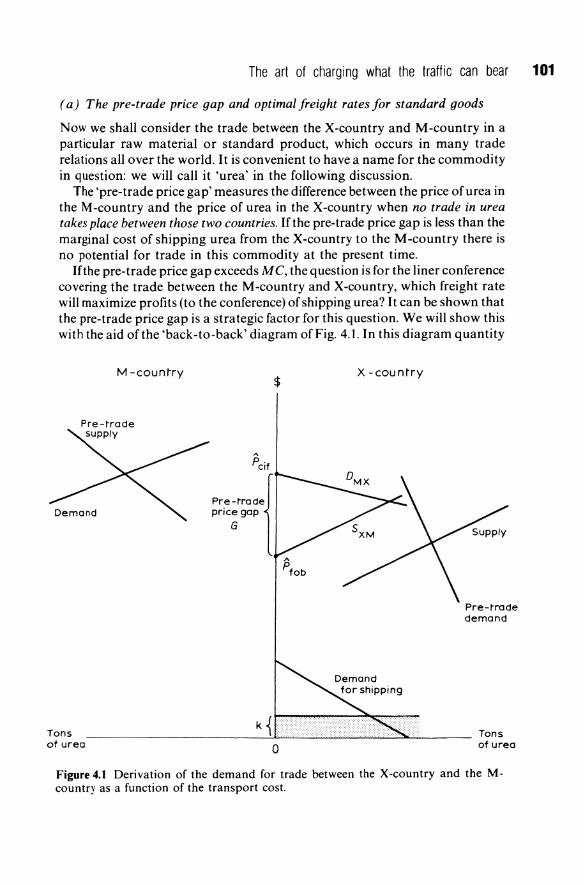
The art of charging what the traffic can bear 101
(a) The pre-trade price gap and optimal freight rates for standard goods
Now we shall consider the trade between the X-country and M-country in a particular raw material or standard product, which occurs in many trade relations all over the world. It is convenient to have a name for the commodity in question: we will caIl it 'urea' in the following discussion.
The 'pre-trade price gap' measures the difference between the price of urea in the M-country and the price of urea in the X-country when no trade in urea takes place between those two countries. If the pre-trade price gap is less than the marginal cost of shipping urea from the X-country to the M-country there is no potential for trade in this commodity at the present time.
If the pre-trade price gap exceeds Me, the question is for the liner conference covering the trade between the M-country and X-country, which freight rate wiIl maximize profits (to the conference) of shipping urea? It can be shown that the pre-trade price gap is a strategic factor for this question. We will show this with the aid of the 'back-to-back' diagram of Fig. 4.1. In this diagram quantity
M -counrry
Pre-rrade price gap
G
$ X -counrry
Pre-rrade demand
Tons ________________________ ~~~~~~~~~~~ _______ Tons of urea 0 of urea
Figure 4.1 Derivation of the demand for trade between the X-country and the Mcountry as a function of the transport cost.
102 The liner shipping industry
of urea supply and demand of the M-country is measured to the left, and quantity of urea supply and demand of the X-country is measured to the right on the horizontal axis. Supply and demand of the M-country depend on the domestic price in the M-country, Pcif' and supply and demand of the Xcountry depend on the domestic price in the X-country, Pfob'
In the pre-trade situation (so far as urea between the X-country and Mcountry is concerned) the price of urea in the X-country, Pfob' is determined by the intersection of the domestic supply curve of the X-country ('Supply and pre-trade demand' in Fig. 4.1). Similarly, in the pre-trade situation the price of urea in the M-country, Pcif' is determined by the intersection of the domestic demand curve of the M-country and the curve for the total supply from possible domestic sources as well as foreign sources except for the X-country ('Demand' and 'Pre-trade supply' in Fig. 4.1).
The supply curve for export of urea from the X-country to the M-country denoted SXM in Fig. 4.1, is derived by subtracting horizontally the pre-trade demand quantity from the supply quantity for each given price in the Xcountry. Similarly, the demand curve for import of urea to the M-country from the X-country, denoted DMX in Fig. 4.1, is derived by subtracting horizontally the domestic demand quantity from the pre-trade supply quantity for each given price in the M-country.
The demand for trade in urea between the X-country and the M-country, DQ, as a function of the total transport cost is in turn derived by taking the vertical difference between DMX and SXM for each given volume of trade.
The demand for shipping of urea, finally, as a function of the freight rate is obtained by moving up the quantity axis to the level of the 'cost, insurance' constant k. Although the urea demand and supply in the M-country and Xcountry are not necessarily linear in their whole ranges, it is a reasonable assumption to regard DMX and SXM and thus the shipping demand curve, which correspond to limited segments of the urea demand and supply curves, as linear. The exact shapes of DMX and SXM can never be established; a linear form is, a priori, the most sensible choice.
After trade has been established, the price of urea changes both in the Mcountry and the X-country. The level of the new prices, Pcif and Pfob depends on the volume of urea trade, Q, that will be moving between the two countries. Let rx represent the (negative) slope of DMX and f3 the slope of SXM' Then the relationships between Pcif and Pfob, respectively, and the trade volume, Q, can be written:
P Cif = PCif - rxQ
Pfob = PfOb + f3Q.
(4.8)
(4.9)
The freight rate, F, equals the difference between P cif and Pfob minus k. The relationship between F and Q is obtained by subtracting equation (4.9) from equation (4.8). The pre-trade price gap is denoted G, which equals the
The art of charging what the traffic can bear 103
difference between P cif and P fob (see Fig. 4.1)
F = Pdf - P fOb - (ex + f3)Q - k
= G - (ex + f3)Q - k. (4.10)
For profit maximization on the part ofthe liner conference it is required that the marginal freight revenue is equal to the marginal cost, Me.
The marginal freight revenue is obtained by taking the derivative of the product FQ with respect to Q
o(FQ) -aQ = G - 2(ex + f3)Q - k. (4.11)
Setting equation (4.11) equal to the marginal shipping cost, MC, and using equation (4.10) to eliminate Q, the optimal freight rate, F*, can be expressed in this way:
F*= G-k+MC 2 . (4.12)
An exceedingly handy rule-of-thumb has been obtained. The optimal freight rate should be equal to the mean of the pre-trade price gap minus k and the marginal shipping cost. This makes sense: If G - k is just above MC there is obviously very little room for a 'contribution margin', for the shipping lines on this particular commodity. The freight rate has to be close to the marginal cost. If G is well above M C, on the other hand, there is room for a good margin. It would be unwise to add such a substantial margin to the marginal cost that the whole pre-trade price gap is exploited. That would kill the trade potential. It would be equally unwise (for profit maximization) to set the freight rate close to the marginal cost. That would make the most of the trade potential, but it would not help shipping profits. A solo monic compromise between these two extremes is apparently the right solution.
Problems of application of this simple rule-of-thumb will arise as soon as the pre-trade stage is far back in the past. When trade in urea between the Xcountry and the M-country has been taking place for a long time, the pre-trade price gap, G, is a hypothetical magnitude, which can be very difficult to estimate. The value of G, say 10 years ago, may have little relevance for the present time. In such a case, how can it be checked that the actual freight rate, F, does not deviate from the profit-maximizing freight rate F*?
(b) The importance of the share of the trade in the total consumption of the importing country, and in the total production of the exporting country
The share of the X-country's export to the M-country, (a) in the total consumption of urea in the M-country, and (b) in the total production of urea in the X-country are two important magnitudes to consider in this connection.
104 The liner shipping industry
From elementary price theory it follows that, if the former share is small, a withdrawal of the supply of urea from the X-country would affect the price of urea in the M-country very little, if at all. If the latter share is small also, it means, similarly, that if the M-country stops importing urea from the Xcountry, it would affect the price of urea in the X-country very little, if at all. The pre-trade price gap is likely to be only slightly larger than the current difference in price of urea between the M-country and the X-country. In these circumstances it is apparent that an increase in the current freight rate for urea could easily result in a complete loss of the urea trade; the demand for shipping urea is likely to be very elastic. Under this condition a decrease in freight rate is the only possibility worth considering, unless, of course, the freight rate already is close to the shipping marginal cost.
If the urea trade from the X-country to the M-country constitutes a relatively large market share in the importing country and/or share in the production, it can be very difficult to predict what the pre-trade price gap would be. There is, unfortunately, no short-cut to the estimation problem of tracing the pre-trade supply and demand curves of the M-country, and the pretrade demand and supply curves of the X-country.
4.3.2 Estimation of import and shipping demand in the case of monopolistic markets for the traded goods
The core of liner cargo is normally constituted by more or less differentiated finished products. Products which are customarily assigned to this category, but which have a number of close substitutes, are probably best dealt with by means of the approach just outlined focusing on the pre-trade price gap. Processed food can be an example of this type of product. When it comes to products which are more markedly differentiated this approach will not do, simply because a 'market price' as distinct from the price of the differentiated product concerned is very difficult, or impossible to identify.
If a certain type of machinery - 'special machinery' from now onproduced in the X-country and exported to the M-country is withdrawn from
this trade, a pre-trade price of special machinery would not exist, because the product in question would not exist in the X-country. It is important for the liner conference, when rate-making, to bear in mind the fact that (by definition) the exporter of special machinery faces a downward-sloping demand curve for his product in the M-country (rather than a given price as in the standardgoods case). The exporter of special machinery has a still greater incentive than the liner conference to estimate the demand for his product in the M-country. The shipping lines in the trade concerned serve exporters of hundreds of heterogeneous products. Each of these exporters should have information on the price elasticity of each particular product of a far more profound nature than the conference rate-makers could ever produce on their own. Therefore, a seemingly natural procedure would be for the conference rate-makers to
The art of charging what the traffic can bear 105
gather the required information en demand in the M-country from the exporters of the X-country.
Conferences do try to get as much relevant information as possible from exporters/importers with a bearing to the elasticity of demand for import. A common practice is that shippers are told that if something happens which threatens the trade in a particular product, the conference is open for discussing the current freight rate. In these discussions the conference is in a position to obtain a lot of useful information. Most rate changes take the form of across-the-board rises by a common percentages. Some articles may, however, be exempted from a general rise, if shippers can give convincing reasons for the necessity of making an exception. For example, the North Atlantic/UK Freight Conference used to request certain information from shippers, whenever an application for rate modifications was made. The shipper concerned was asked to provide information on whether the product in question was hazardous, the nature, size, and weight of packages, the value and the duty, the point of origin and destination, the anticipated volume of total shipments, as well as information on competitive products and their prices (Federal Maritime Commission 1968).
The general problem is, of course, that rate-makers and shippers have sharply conflicting interests when it comes to the crucial matter of what the traffic can bear. If the demand for special machinery in the M-country is rather inelastic the producer of special machinery could earn a handsome profit on the export to the M-country - the price charged in the M-country could exceed the marginal cost of production by a substantial margin. If the liner conference were aware of this fact they could get a substantial share of the cake. The exporter is not very keen to disclose anything which could lead to this. In discussions with the conference the exporter is more likely to overestimate the price elasticity by pointing out all sorts of factors speaking against the supposition that special machinery can bear a very high freight rate.
(a) Indirect way of getting at the demand elasticity via the exporter's profit margin
There are, however, some possibilities of getting some information on the exporter's view on the price elasticity without having to ask him directly.
Were it known what the (marginal) cost of production of special machinery is, the size of the profit margin on export to the M-country would be quite revealing. Presuming profit-maximization on the part of the exporter, one has simply to apply the general relationship between price, marginal revenue, and demand elasticity: ED = P/(MR - P). Substituting Me of production (including other transport costs than the shipping freight rate, that is, k) for M R, a value for ED is obtained.
The problem with this approach is that the marginal cost of production can be difficult to ascertain for an outsider. It may be thought that the fob price or
106 The liner shipping industry
the domestic price in the exporter's home country could be used as an M C proxy. This would be fine in a constant-cost industry. Assuming constant returns to scale is convenient, but hardly generally justified so far as monopolistic and oligopolistic industries are concerned. Decreasing returns to scale, and rising supply curves are to be found almost exclusively in the primary goods sector, i.e. in the extraction industries (mining etc.), agriculture, fishing and forestry. However, increasing returns to scale is the rule rather than the exception in the manufactured-goods sector, and in this case it can be very difficult to infer from Prob where the level of MC may be.
4.3.3 The tolerance level of freight rates for firms selling in oligopolistic markets
So far we have assumed monopoly or monopolistic competition so far as the goods markets are concerned. Exporters of manufactured goods often perceive the foreign markets where they are selling as oligo polis tic. The characteristic of this market form is that each individual seller believes his present market share cannot be increased simply by a price cut, because all the others will follow suit, while a price rise may be disastrous for his market share, as it then can be expected that the others will stay put. This is the well-known case of the kinked demand curve. In this case a shift in the marginal cost of an individual seller will in a wide range have no effect at all on price or quantity supplied, but the seller in question will either simply absorb the cost increase by accepting a lower profit margin or he will succeed in finding a way of offsetting the cost increase, for example by factor substitution.
For the liner conference the question is, when it comes to exporters selling in oligopolistic markets, which freight rate levels can they absorb before they seriously look around for an alternative mode of transport?
In the economically imperfect world we are living in, it is not always true that the price of manufactured goods is equal to the average cost including a normal profit to the owner. Profits vary widely between firms in practice. In cases where super-normal profits are earned, there are better odds for a relatively high freight rate to be accepted than in cases where profit margins are pressed. It is not always possible to obtain reliable information about profit margins. In that case it is close to hand to use product value as a proxy for freight-rate tolerance. Were profit margins proportional, on average, to product prices, this would not be unreasonable. However, on second thought it should be clear that profit per unit of output is more likely to be proportional to the capital cost content in prices. Returns on capital investment minus costs of debt servicing is equal to gross profit. The labour cost content and the input goods cost content in prices, per se, should normally not be related to profit per unit of output. Therefore a superior rule-of-thumb seems to be to take the capital cost content rather than the whole price as a proxy for the willingness to absorb freight costs.
The substitution possibilities as regards the shipping services are obviously
The art of charging what the traffic can bear 107
also of vital importance for the 'tolerance level' of freight rates. We now turn to the second type of competition which is often the most important reason for liner shipping demand being far more elastic than is suggested by just looking at the trade potential.
4.4 COMPETITION FROM 'OUTSIDERS' AND OTHER MODES OF TRANSPORT (SEE ALSO DISCUSSION IN SECTION 2.2.2)
So far as the shipping services offered by liner conference members are concerned, the main source of competition is perhaps that from other lines. That the 'seas are open' is more than a phrase. If a conference raises freight rates so that the trade route becomes very remunerative, other lines will be attracted into the trade - either by forcing their way into the conference, or by operating as 'outsiders'. The threat of potential entrants into the trade is a permanent one, and sets a limit in the first place to the general level offreight rates.
Tramps and specialized bulk-carriers form another source of competition. They mainly compete on the bulk cargo, when the size of the shipment is sufficient to fill a ship. The great bargaining power of big shippers forces down the rates of bulk commodities. Conferences, therefore, often declare rates of these commodities 'open', or else fix the freight rates close to the corresponding tramp rates. Bulk cargo can be important for some liner services. It usually serves to fill gaps in the availability of break-bulk cargo - on the backhaul, or in off-peak periods. The growing use of chartered ships for consolidated parcels of minor bulk commodities, 'neo-bulk shipping', and the possibility of tramps topping up their base cargo (i.e. bulk cargo) with break-bulk cargo have the effect in some trades of extending the impact of tramp competition to most commodities carried there.
Airline competition is a third source that limits the possibility of the conferences to raise freight rates. Technical developments in the airline industry have made competition with liner shipping more intense. Airlines mostly compete on high-value commodities. They are therefore a threat to the 'cream' of the liner trade. (It has been estimated that in 1969 air cargo accounted for 22% of the total dollar value of all foreign trade moving through the New York Boat district, although it comprised less than 1 % of the total tonnage. Madden (1970; p. I). In 1970 air cargo accounted for 16.6% of the value of US exports and 9.4% of the imports value, see McCaul (1970).
4.5 SUMMARY AND CONCLUSIONS
The preceding analysis of the freight-rate elasticity of demand for liner shipping of different commodities can be summarized with reference to Fig. 4.2.
We have discussed the problem in three stages. First we have shown that by
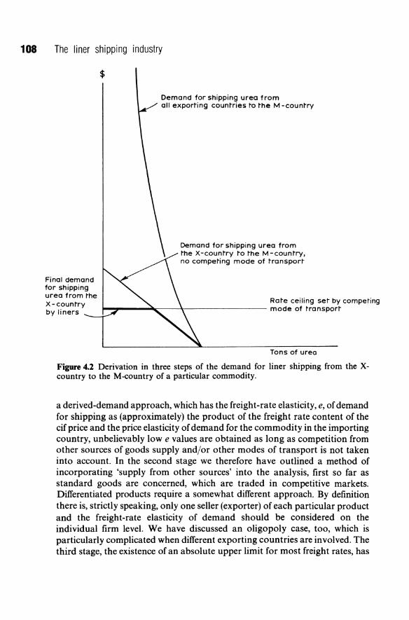
108 The liner shipping industry
Final demand for shipping urea from ~he X-coun~ry
by liners
$
Demand for shipping urea from all expor~ing coun~ries ~o ~he M -coun~ry
Demand for shipping urea from ~he X-coun~ry ~o ~he M-coun~ry,
no compe~ing mode of ~ranspor~
Ra~e ceiling se~ by competing I-..,..--..... ~--\-------- mode of transpor~
Tons of urea
Figure 4.2 Derivation in three steps of the demand for liner shipping from the xcountry to the M-country of a particular commodity.
a derived-demand approach, which has the freight-rate elasticity, e, of demand for shipping as (approximately) the product of the freight rate content of the cif price and the price elasticity of demand for the commodity in the importing country, unbelievably lowe values are obtained as long as competition from other sources of goods supply and/or other modes of transport is not taken into account. In the second stage we therefore have outlined a method of incorporating 'supply from other sources' into the analysis, first so far as standard goods are concerned, which are traded in competitive markets. Differentiated products require a somewhat different approach. By definition there is, strictly speaking, only one seller (exporter) of each particular product and the freight-rate elasticity of demand should be considered on the individual firm level. We have discussed an oligopoly case, too, which is particularly complicated when different exporting countries are involved. The third stage, the existence of an absolute upper limit for most freight rates, has

The art of charging what the traffic can bear 109
been recognized. Depending on the category of cargo, this limit is set by competing 'outsiders' (shipping lines operating outside conferences), tramps, or air cargo carriers.
One important qualification of the previous conclusion about the importance of commodity value for freight rates has come out. The value of products cannot be regarded as a direct factor of great importance for the freight-rate making. For mainly two reasons the freight rates are none the less positively correlated to the value of the traded goods, namely:
Due to competition from tramps and neo-bulk carriers, the average freight rate ceiling is typically much lower for primary goods than for more valuable processed goods.
2 As freight rates are expected to be related to the (absolute) profit margins, they should also be related to the prices (commodities) of the products concerned. The relationship between price and profit margin is, however, an indirect one. The profit margin should be more directly associated with the part of the value added represented by the capital cost. *
*For example, the profit margin per motor car sold from a car-parts assembly plant is normally much lower than the profit margin per motor car sold from a fully integrated car-making plant. The exporter/producer's capital cost per product unit can be expected to be increasing at a markedly degressive rate with increases in the total value (price) per product unit, because the more valuable a product is, the more process stages it is likely to have passed, and the smaller proportion of the total value is likely to have been added by the exporter/producer.
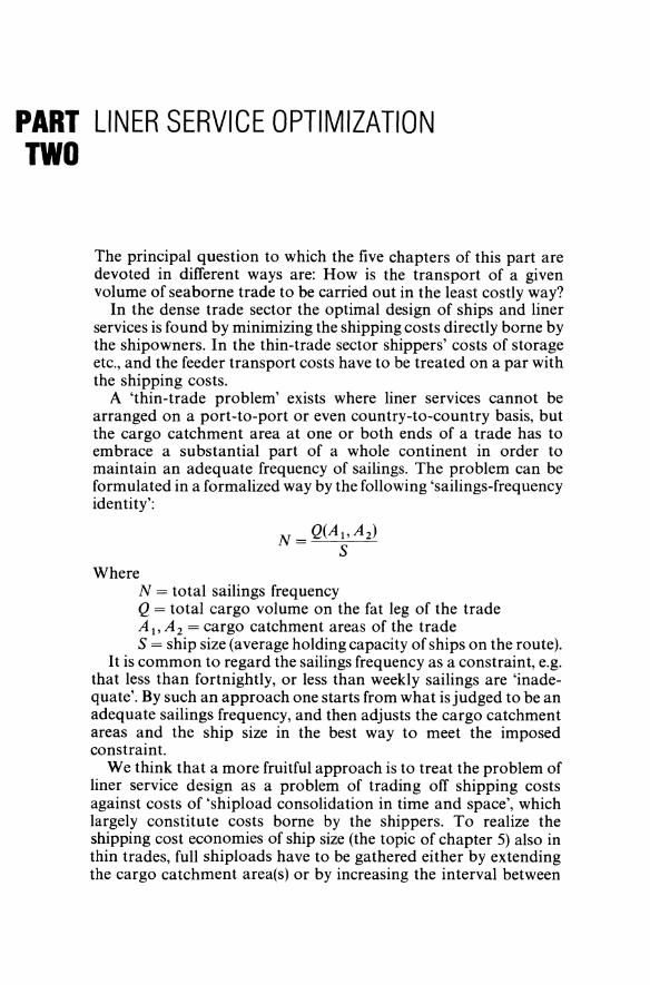
PART LINER SERVICE OPTIMIZATION TWO
The principal question to which the five chapters of this part are devoted in different ways are: How is the transport of a given volume of seaborne trade to be carried out in the least costly way?
In the dense trade sector the optimal design of ships and liner services is found by minimizing the shipping costs directly borne by the shipowners. In the thin-trade sector shippers' costs of storage etc., and the feeder transport costs have to be treated on a par with the shipping costs.
A 'thin-trade problem' exists where liner services cannot be arranged on a port-to-port or even country-to-country basis, but the cargo catchment area at one or both ends of a trade has to embrace a substantial part of a whole continent in order to maintain an adequate frequency of sailings. The problem can be formulated in a formalized way by the following 'sailings-frequency identity':
Where N = total sailings frequency Q = total cargo volume on the fat leg of the trade A1, A2 = cargo catchment areas of the trade S = ship size (average holding capacity of ships on the route).
It is common to regard the sailings frequency as a constraint, e.g. that less than fortnightly, or less than weekly sailings are 'inadequate'. By such an approach one starts from what is judged to be an adequate sailings frequency, and then adjusts the cargo catchment areas and the ship size in the best way to meet the imposed constraint.
We think that a more fruitful approach is to treat the problem of liner service design as a problem of trading off shipping costs against costs of 'shipload consolidation in time and space', which largely constitute costs borne by the shippers. To realize the shipping cost economies of ship size (the topic of chapter 5) also in thin trades, full shiploads have to be gathered either by extending the cargo catchment area(s} or by increasing the interval between
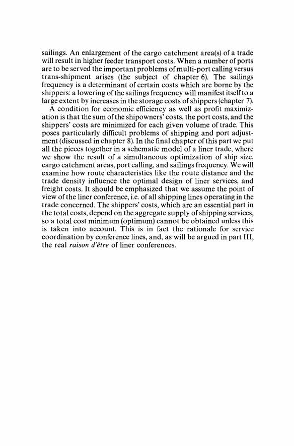
sailings. An enlargement of the cargo catchment area(s) of a trade will result in higher feeder transport costs. When a number of ports are to be served the important problems of multi-port calling versus trans-shipment arises (the subject of chapter 6). The sailings frequency is a determinant of certain costs which are borne by the shippers: a lowering of the sailings frequency will manifest itself to a large extent by increases in the storage costs of shippers (chapter 7).
A condition for economic efficiency as well as profit maximization is that the sum of the shipowners' costs, the port costs, and the shippers' costs are minimized for each given volume of trade. This poses particularly difficult problems of shipping and port adjustment (discussed in chapter 8). In the final chapter of this part we put all the pieces together in a schematic model of a liner trade, where we show the result of a simultaneous optimization of ship size, cargo catchment areas, port calling, and sailings frequency. We will examine how route characteristics like the route distance and the trade density influence the optimal design of liner services, and freight costs. It should be emphasized that we assume the point of view of the liner conference, i.e. of all shipping lines operating in the trade concerned. The shippers' costs, which are an essential part in the total costs, depend on the aggregate supply of shipping services, so a total cost minimum (optimum) cannot be obtained unless this is taken into account. This is in fact the rationale for service coordination by conference lines, and, as will be argued in part III, the real raison d'etre of liner conferences.
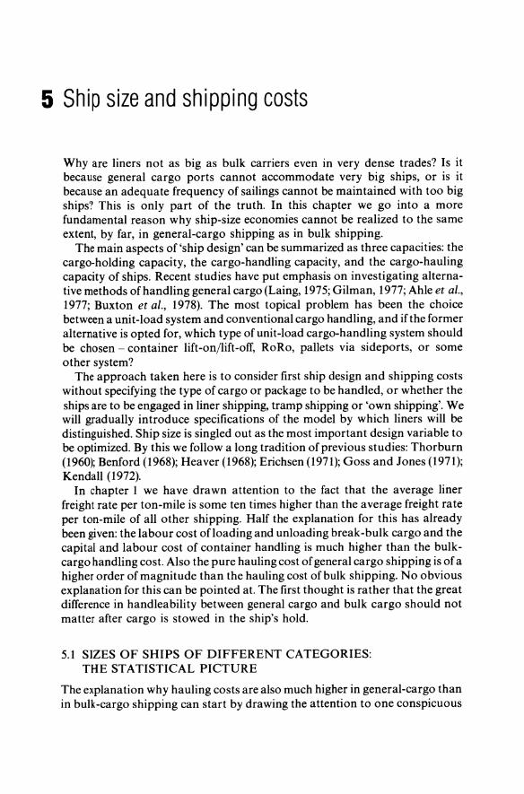
5 Ship size and shipping costs
Why are liners not as big as bulk carriers even in very dense trades? Is it because general cargo ports cannot accommodate very big ships, or is it because an adequate frequency of sailings cannot be maintained with too big ships? This is only part of the truth. In this chapter we go into a more fundamental reason why ship-size economies cannot be realized to the same extent, by far, in general-cargo shipping as in bulk shipping.
The main aspects of 'ship design' can be summarized as three capacities: the cargo-holding capacity, the cargo-handling capacity, and the cargo-hauling capacity of ships. Recent studies have put emphasis on investigating alternative methods of handling general cargo (Laing, 1975; Gilman, 1977; Ahle et al., 1977; Buxton et al., 1978). The most topical problem has been the choice between a unit-load system and conventional cargo handling, and if the former alternative is opted for, which type of unit-load cargo-handling system should be chosen - container lift-on/lift-off, RoRo, pallets via sideports, or some other system?
The approach taken here is to consider first ship design and shipping costs without specifying the type of cargo or package to be handled, or whether the ships are to be engaged in liner shipping, tramp shipping or 'own shipping'. We will gradually introduce specifications of the model by which liners will be distinguished. Ship size is singled out as the most important design variable to be optimized. By this we follow a long tradition of previous studies: Thorburn (1960); Benford (1968); Heaver (1968); Erichsen (1971); Goss and Jones (1971); Kendall (1972).
In chapter 1 we have drawn attention to the fact that the average liner freight rate per ton-mile is some ten times higher than the average freight rate per ton-mile of all other shipping. Half the explanation for this has already been given: the labour cost ofloading and unloading break-bulk cargo and the capital and labour cost of container handling is much higher than the bulkcargo handling cost. Also the pure hauling cost of general cargo shipping is of a higher order of magnitude than the hauling cost of bulk shipping. No obvious explanation for this can be pointed at. The first thought is rather that the great difference in handleability between general cargo and bulk cargo should not matter after cargo is stowed in the ship's hold.
5.1 SIZES OF SHIPS OF DIFFERENT CATEGORIES: THE STATISTICAL PICTURE
The explanation why hauling costs are also much higher in general-cargo than in bulk-cargo shipping can start by drawing the attention to one conspicuous

114 Liner service optimization
difference between general-cargo and bulk-cargo shipping: the size of ships. In Table 5.1 the average sizes of tankers, dry-bulk carriers, container ships,
and conventional general-cargo ships are given. Since the development of ship sizes of the two former categories has been very dynamic in recent years, a time series of figures are presented. In the liner sector the only more important change in ship size that has taken place latterly is the steady growth of the average size of container ships during the 1970s.
These average figures hide, for every ship category, a very wide span of variations in ship sizes. Oil tankers of 500 000 dwt exist, but tanker sizes range down to below 1000 dwt, and the spread is fairly even in terms of numbers of ships. No very pronounced concentration to a particular size range can be discerned. The same pattern applies to the dry-bulk carriers, although the maximum ship size in this category is half that of tankers.
Table 5.1 Average size of ships of different categories
Conventional Dry bulk Container general-
Date Tankers' carriers' Date shipb cargo shipsb
1/1/64 26147 20284 1/7/70 11425 3268 1/1/65 28123 21046 1/7/71 12038 3266 1/1/66 30478 22553 1/7/72 13 814 3259 1/1/67 32902 23996 1/7/73 14972 3249 1/1/68 35211 25834 1/7/74 15269 3248 1/1/69 38304 26916 1/7/75 14902 3296 1/1/70 42985 27596 1/7/76 15091 3391 1/1/71 48060 28484 1/7/77 14878 3494 1/1/72 52526 29552 1/7/78 16335 3561 1/1/73 58252 30465 1/7/79 16868 3591 1/1/74 64439 31643 1/7/80 17030 3593 1/1/75 73487 32185 1/7/81 17386 3602 1/1/76 83973 32599 1/7/82 18025 3576 1/1/77 90682 33366 1/7/83 18197 3556 1/1/78 98941 34024 1/1/79 103762 34250 1/1/80 104603 34468 1/1/81 103403 34679 1/1/82 102376 35462 1/1/83 101 733 36509
Source: Various issues of Drewry (Shipping statistics and economics, H.P. Drewry, Shipping Consultant, Ltd.) Lloyd's Register of Shipping, Statistical Tables, 1970-83.
"Total dwt of ships greater than 10000 dwt divided by number of ships in the category. "Total GRT of ships greater than 100 GRT divided by the number of ships in the category.
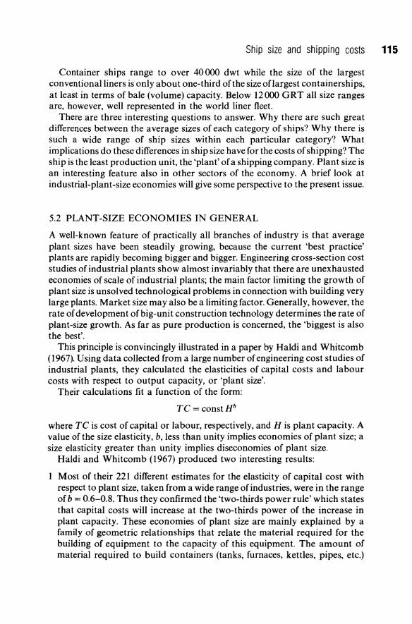
Ship size and shipping costs 115
Container ships range to over 40000 dwt while the size of the largest conventional liners is only about one-third of the size oflargest containerships, at least in terms of bale (volume) capacity. Below 12000 GRT all size ranges are, however, well represented in the world liner fleet.
There are three interesting questions to answer. Why there are such great differences between the average sizes of each category of ships? Why there is such a wide range of ship sizes within each particular category? What implications do these differences in ship size have for the costs of shipping? The ship is the least production unit, the 'plant' of a shipping company. Plant size is an interesting feature also in other sectors of the economy. A brief look at industrial-plant-size economies will give some perspective to the present issue.
5.2 PLANT-SIZE ECONOMIES IN GENERAL
A well-known feature of practically all branches of industry is that average plant sizes have been steadily growing, because the current 'best practice' plants are rapidly becoming bigger and bigger. Engineering cross-section cost studies of industrial plants show almost invariably that there are unexhausted economies of scale of industrial plants; the main factor limiting the growth of plant size is unsolved technological problems in connection with building very large plants. Market size may also be a limiting factor. Generally, however, the rate of development of big-unit construction technology determines the rate of plant-size growth. As far as pure production is concerned, the 'biggest is also the best'.
This principle is convincingly illustrated in a paper by Haldi and Whitcomb (1967). Using data collected from a large number of engineering cost studies of industrial plants, they calculated the elasticities of capital costs and labour costs with respect to output capacity, or 'plant size'.
Their calculations fit a function of the form:
TC= constHb
where TC is cost of capital or labour, respectively, and H is plant capacity. A value of the size elasticity, b, less than unity implies economies of plant size; a size elasticity greater than unity implies diseconomies of plant size.
Haldi and Whitcomb (1967) produced two interesting results:
1 Most of their 221 different estimates for the elasticity of capital cost with respect to plant size, taken from a wide range of industries, were in the range of b = 0.6-0.8. Thus they confirmed the 'two-thirds power rule' which states that capital costs will increase at the two-thirds power of the increase in plant capacity. These economies of plant size are mainly explained by a family of geometric relationships that relate the material required for the building of equipment to the capacity of this equipment. The amount of material required to build containers (tanks, furnaces, kettles, pipes, etc.)
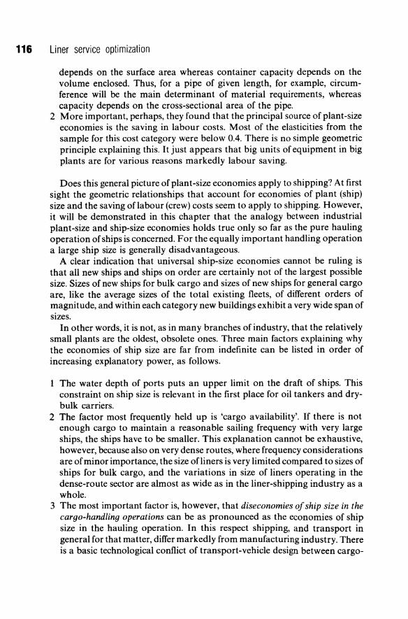
116 Liner service optimization
depends on the surface area whereas container capacity depends on the volume enclosed. Thus, for a pipe of given length, for example, circumference will be the main determinant of material requirements, whereas capacity depends on the cross-sectional area of the pipe.
2 More important, perhaps, they found that the principal source of plant-size economies is the saving in labour costs. Most of the elasticities from the sample for this cost category were below 0.4. There is no simple geometric principle explaining this. It just appears that big units of equipment in big plants are for various reasons markedly labour saving.
Does this general picture of plant-size economies apply to shipping? At first sight the geometric relationships that account for economies of plant (ship) size and the saving of labour (crew) costs seem to apply to shipping. However, it will be demonstrated in this chapter that the analogy between industrial plant-size and ship-size economies holds true only so far as the pure hauling operation of ships is concerned. For the equally important handling operation a large ship size is generally disadvantageous.
A clear indication that universal ship-size economies cannot be ruling is that all new ships and ships on order are certainly not of the largest possible size. Sizes of new ships for bulk cargo and sizes of new ships for general cargo are, like the average sizes of the total existing fleets, of different orders of magnitude, and within each category new buildings exhibit a very wide span of sizes.
In other words, it is not, as in many branches of industry, that the relatively small plants are the oldest, obsolete ones. Three main factors explaining why the economies of ship size are far from indefinite can be listed in order of increasing explanatory power, as follows.
1 The water depth of ports puts an upper limit on the draft of ships. This constraint on ship size is relevant in the first place for oil tankers and drybulk carriers.
2 The factor most frequently held up is 'cargo availability'. If there is not enough cargo to maintain a reasonable sailing frequency with very large ships, the ships have to be smaller. This explanation cannot be exhaustive, however, because also on very dense routes, where frequency considerations are of minor importance, the size ofliners is very limited compared to sizes of ships for bulk cargo, and the variations in size of liners operating in the dense-route sector are almost as wide as in the liner-shipping industry as a whole.
3 The most important factor is, however, that diseconomies of ship size in the cargo-handling operations can be as pronounced as the economies of ship size in the hauling operation. In this respect shipping, and transport in general for that matter, differ markedly from manufacturing industry. There is a basic technological conflict of transport-vehicle design between cargo-
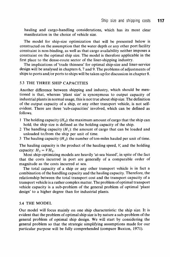
Ship size and shipping costs 117
hauling and cargo-handling considerations, which has its most clear manifestation in the choice of vehicle size.
The model for ship-size optimization that will be presented below is constructed on the assumption that the water depth or any other port facility constraint is non-binding, as well as that cargo availability neither imposes a constraint on the optimal ship size. The model is therefore applicable in the first place to the dense-route sector of the liner-shipping industry.
The implications of 'trade thinness' for optimal ship-size and liner-service design will be analysed in chapters 6, 7 and 9. The problems of adjustments of ships to ports and/or ports to ships will be taken up for discussion in chapter 8.
5.3 THE THREE SHIP CAPACITIES
Another difference between shipping and industry, which should be mentioned is that, whereas 'plant size' is synonymous to output capacity of industrial plants in normal usage, this is not true about ship size. The definition of the output capacity of a ship, or any other transport vehicle, is not selfevident. There are three 'sub-capacities' involved, which can be defined as follows.
The holding capacity (H 0): the maximum amount of cargo that the ship can hold; the ship size is defined as the holding capacity of the ship.
2 The handling capacity (H 1): the amount of cargo that can be loaded and unloaded to/from the ship per unit of time.
3 The hauling capacity (H 2): the number of ton-miles hauled per unit of time.
The hauling capacity is the product of the hauling speed, V, and the holding capacity: H2 = VHo·
Most ship-optimizing models are heavily 'at-sea biased', in spite of the fact that the costs incurred in port are generally of a comparable order of magnitude as the costs incurred at sea.
The total capacity of a ship or any other transport vehicle is in fact a combination of the handling capacity and the hauling capacity. Therefore, the relationship between the total transport cost and the transport capacity of a transport vehicle is a rather complex matter. The problem of optimal transport vehicle capacity is a sub-problem of the general problem of optimal 'plant design' to a higher degree than for industrial plants.
5.4 THE MODEL
Our model will focus mainly on one ship characteristic: the ship size. It is evident that the problem of optimal ship size is by nature a sub-problem of the general problem of optimal ship design. We will start by considering the general problem so that the strategic simplifying assumptions made for our particular purpose will be fully comprehended (compare Buxton, 1971).

118 Liner service optimization
5.4.1 The general problem of optimal ship design
On a dense route where the cargo base is sufficiently substantial not to impose a constraint on the choice of ship design, the optimal ship for the route concerned is defined as the ship that carries cargo of a given composition at the lowest total cost for the shipowner per cargo ton. With this definition there is no need to treat the total number of ships on the route as an independent variable; given the optimal ship, the required total number of ships follows from this and the total volume of cargo to be carried. The route where the ships to be optimized are to be employed is specified by the cargo composition, the directional cargo balance, the route distance, and the characteristics of the ports of call, which can be symbolized by a vector X. The ship-design variables to be optimized are denoted without further specification by the vector Y.
The three ship capacities, H 0, Hi and H 2> as well as the factor costs - ship capital cost, costs of crew, fuel, stevedoring labour etc. - are determined by the design variables, and, in the case of the handling capacity and the costs incurred in port, by the port characteristics in addition.
Ho = Ho(Y)
Hi = Hi(Y,X)
H2=HoV(Y)
The total shipping cost can be divided into two main categories: so-called cargo costs which are by and large proportional to the cargo quantity, and costs which are time-proportional. To the latter category we assign also the fuel cost. This cost is otherwise commonly referred to as a category of its own; it is naturally regarded as miles-proportional, but, given the speed a milesproportional cost can just as soon be treated as a time-proportional cost.
The time-proportional costs incurred in port, and at sea, respectively, are not completely overlapping. The cost offuel is the most important cost, which is (practically) only incurred at sea, and lay-time proportional port charges are only incurred Import. We therefore make this notational distinction: the ith factor cost is in all cases incurred in port, and in some cases at sea, too, and the jth factor cost is in all cases incurred at sea, and in some cases it is incurred in port, too.
Total time cost per day in port = I,J;(X, Y,pJ i
Total time cost per day at sea = I,fiY,p) i
Total cargo cost per ton of cargo, C 3 = I, fk(X, V). k
In the functions for the time-proportional factor costs the applicable factor prices, Pi and Pi' respectively, are also included as arguments. The cargo costs appear to the shipowner as various charges; from the shipowner's point of
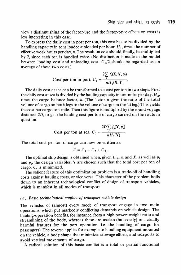
Ship size and shipping costs 119
view a distinguishing of the factor-use and the factor-price effects on costs is less interesting in this case.
To express the daily cost in port per ton, this cost has to be divided by the handling capacity in tons loaded/unloaded per hour, H l' times the number of effective work hours per day, n. The resultant cost should, finally, be multiplied by 2, since each ton is handled twice. (No distinction is made in the model between loading cost and unloading cost. C d2 should be regarded as an average of these two costs.)
2L:!;(X, Y,Pi) Cost per ton in port, C 1 = --'-i ___ _
nH 1(X, Y) .
The daily cost at sea can be transformed to a cost per ton in two steps. First the daily cost at sea is divided by the hauling capacity in ton-miles per day, H 2,
times the cargo balance factor, Ji. (The factor Ji gives the ratio of the total volume of cargo on both legs to the volume of cargo on the fat leg.) This yields the cost per cargo ton-mile. Then this figure is multiplied by the round voyage distance, 2D, to get the hauling cost per ton of cargo carried on the route in question.
2DL:fiY ,p) Cost per ton at sea, C 2 = _--oJ,---. --
JiH z(Y)
The total cost per ton of cargo can now be written as:
C = C 1 + C2 + C3 .
The optimal ship design is obtained when, given D, Ji, n, and X, as well as Pi and Pj' the design variables, Yare chosen such that the total cost per ton of cargo, C, is minimized.
The salient feature of this optimization problem is a trade-off of handling costs against hauling costs, or vice versa. This character of the problem boils down to an inherent technological conflict of design of transport vehicles, which is manifest in all modes of transport.
( a) Basic technological conflict oj transport vehicle design
The vehicles of (almost) every mode of transport engage in two main operations, which put markedly conflicting demands on vehicle design. The hauling-operation benefits, for instance, from a high power: weight ratio and streamlining of the body, whereas these are useless (but costly) or actually harmful features for the port operation, i.e. the handling of cargo (or passengers). The reverse applies for example to handling equipment mounted on the vehicle, a body shape that minimizes stowage efforts, and sideports to avoid vertical movements of cargo.
A radical solution of this basic conflict is a total or partial functional

120 Liner service optimization
Table 5.2 Groups of ship design variables which determine the ship capacities
Capacity determinants
Main dimensions Main dimensions, access to holds,
cargo gear on ship, port facilities Main dimensions, machinery, access
to holds, cargo gear on ship
Capacities
decomposition of the vehicle 'unit'. Railway transport, where the locomotive of a train of freight wagons can be uncoupled and employed elsewhere during the loading and unloading of the wagons, tractors and trailers, tugs and barges, are the most common cases in point. The lighter-aboard-ship (LASH) system is a modern variant of this principle. The characteristic feature of a container transport system is that the most time-consuming part of the loading and unloading operations ~ the stuffing and stripping of the containers ~ is performed when the container ship is engaged in hauling operations. The loading on the ship and the discharge of the filled containers take only a fraction of the time which would be required if the various articles were stowed directly into the ship. If one regards the containers as integral parts of the container ship, the idea of containerization is clearly another variant of the 'tugs and barges' solution to the basic conflict of transportvehicle design.
Disregarding the possibility of a functional decomposition of the vehicle, the typical result of the conflicting demands is a vehicle design which is a compromise between handling and hauling considerations.
The ship design variables, Y can be classified in four broad groups, ship's main dimensions, design of the access to holds, type of cargo gear on ship, and machinery, which can be distinguished as determinants of one or more of the ship capacities according to Table 5.2.
In choosing the main dimensions of a ship, the horsepower of the machinery etc., the positive effect on the cost per ton at sea and the negative effect on the cost per ton in port, or vice versa, are to be balanced.
(b) Continuous design variables and class variables
Most of the design variables are continuous, and the question is how much of this or that design characteristic is to be chosen in order to balance the handling and hauling costs? Some important design characteristics can, however, not be expressed by continuous variables; it is a question of either/or. A typical class variable is the engine type: one has either to choose a steam
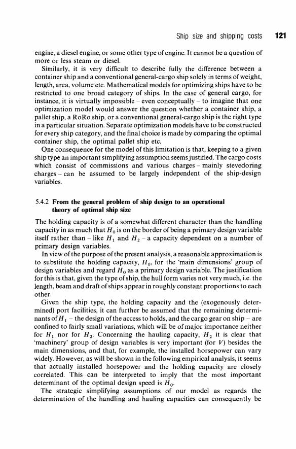
Ship size and shipping costs 121
engine, a diesel engine, or some other type of engine. It cannot be a question of more or less steam or diesel.
Similarly, it is very difficult to describe fully the difference between a container ship and a conventional general-cargo ship solely in terms of weight, length, area, volume etc. Mathematical models for optimizing ships have to be restricted to one broad category of ships. In the case of general cargo, for instance, it is virtually impossible - even conceptually - to imagine that one optimization model would answer the question whether a container ship, a pallet ship, a RoRo ship, or a conventional general-cargo ship is the right type in a particular situation. Separate optimization models have to be constructed for every ship category, and the final choice is made by comparing the optimal container ship, the optimal pallet ship etc.
One consequence for the model of this limitation is that, keeping to a given ship type an important simplifying assumption seems justified. The cargo costs which consist of commissions and various charges - mainly stevedoring charges - can be assumed to be largely independent of the ship-design variables.
5.4.2 From the general problem of ship design to an operational theory of optimal ship size
The holding capacity is of a somewhat different character than the handling capacity in as much that Ho is on the border of being a primary design variable itself rather than -like H 1 and H 2 - a capacity dependent on a number of primary design variables.
In view of the purpose of the present analysis, a reasonable approximation is to substitute the holding capacity, H 0' for the 'main dimensions' group of design variables and regard H 0 as a primary design variable. The justification for this is that, given the type of ship, the hull form varies not very much, i.e. the length, beam and draft of ships appear in roughly constant proportions to each other.
Given the ship type, the holding capacity and the (exogenously determined) port facilities, it can further be assumed that the remaining determinants of H 1 - the design of the access to holds, and the cargo gear on ship - are confined to fairly small variations, which will be of major importance neither for H 1 nor for H 2. Concerning the hauling capacity, H 2 it is clear that 'machinery' group of design variables is very important (for V) besides the main dimensions, and that, for example, the installed horsepower can vary widely. However, as will be shown in the following empirical analysis, it seems that actually installed horsepower and the holding capacity are closely correlated. This can be interpreted to imply that the most important determinant of the optimal design speed is H o.
The strategic simplifying assumptions of our model as regards the determination of the handling and hauling capacities can consequently be
122 Liner service optimization
summarized in this manner. To mark the step from a general ship design optimization model to a model for ship size optimization, the symbol S( = ship size) is replacing H o.
Ho=S
H1 =H 1 (S,X) H2 = SV(S)
Similarly, the time-proportional factor costs incurred in port and at sea are written nS, X, Pj) and liS, p), respectively.
To operationalize the model these relationships have to be specified. Shipbuilding and marine-engineering cost studies have shown that an exponential function is the most suitable form of expressing the relationships between H 1 and H 2, and ship size, as well as between each factor cost and ship size. To an extent this form is a reflection of the fact that certain geometric principles relating volume, surface area, and length are at work. A good example is the cost of painting the hull. This cost is expected to vary in proportion to the surface area of the ship, which in turn is roughly proportional to the two-thirds power of the ship size.
The relationship between handling capacity and size and hauling capacity and size will therefore be expressed as:
H l(S, X) = h 1SE1
H2 = SV(S) = h2SE2
The proportionality constant h1 is specific to each ship type. It also reflects exogenous factors, like cargo composition, port capital and labour productivity. Likewise, h2 is expected to differ among ship types. The exponents E1 and E2 are the elasticities of handling capacity and hauling capacity with respect to ship size.
The basic technological conflict between handling and hauling considerations is expected to manifest itself in a comparatively low value of E l' and in a comparatively high value of E2 : as the ship size is growing the handling capacity is expected to increase much slower than in proportion to S, while the hauling capacity is expected to increase at least in proportion to S.
The time-proportional factor costs are most suitable to write in this way, where factor price and factor use are clearly distinguished.
fj(X, S, pJ = pjqjse;
fj(S,p) = Pjqjse j •
In the case of fuel cost, for instance, Pj represents the price of fuel, and qjsej
represents the fuel consumption per day at sea when cruising at the design speed.
The total time cost in port per ton, C 1, and the total time cost at sea per ton, C 2' are obtained as before, by summing over all i and j, and dividing by the
Ship size and shipping costs 123
handling capacity and hauling capacity respectively, as well as inserting the relevant route characteristics.
2DLPjQjse j
C2 = J.l~2SE2 By including the total cargo costs per ton, C 3' the total cost per ton, C, on the
route concerned can, finally, be written in this form:
(5.1)
Our hypothesis is that economy of ship size is enjoyed in the hauling operation, i.e. that the hauling cost per ton (the second term) is decreasing with increases in ship size. This will be the case if ej - E2 < 0 on balance. On the other hand, we expect that diseconomy of ship size is suffered in the handling operation, i.e. that the handling cost per ton (the first term) is increasing with increases in ship size. This will be the case if ei - E 1 > 0 on balance.
5.5 ESTIMATION OF SHIP SIZE ELASTICITIES OF HANDLING AND HAULING CAPACITIES AND FACTOR COSTS
The values of ei and ej , on one hand, and of E1 and E 2 , on the other hand, are equally important for the issue of (dis)economies of ship size. The relationship between the various factor costs and ship size has been the subject of a number of engineering and economic studies. The least-studied relevant relationship is, strangely enough, that between the handling capacity and ship size, which, as it will appear, is of particular importance for the whole issue of ship size. A notable exception is Professor Thorburn's (1960) study, which includes a tramp-shipping model, in which the observed (by him) markedly diminishing returns to ship size in the handling operation is the strategic ingredient.
In this section we will summarize the empirical evidence with a bearing to the size-elasticities in question that has been produced in previous studies, as well as present the results of the empirical tests of the relationships of our model, which we have been able to make.
5.5.1 The size elasticity of the handling capacity
The time it takes to fill or empty a bathtub of water is proportional to the volume of the tub, given the capacity of the waterpipe or the discharge pipe. The loading or unloading speed in such a case = const So, where S is the size, or

124 Liner service optimization
holding capacity of the tub. This equation implies markedly diminishing returns to size: thus two tubs that are each half as big, but together hold the same amount of water as a large one can be filled and emptied in half the time. There are transport vehicles which suffer similar diminishing returns in their loading and unloading operations. A bus equipped with one entrance and one exit door is a case in point. Freight vehicles are seldom that uneconomically designed. The number of inlets/outlets is, as a rule, increased as the size of the hold becomes larger. The question is: At which rate in relation to the increase in size?
For geometric reasons, it is unconceivable to make the number of inlets/outlets increase in proportion to the volume of the hold. At the very most, they might increase in proportion to the surface area of the hold. In that
2
case the handling capacity could be = const S3. This would still imply diminishing returns to size in the handling operation
(although not necessarily diseconomies of size, as this also depends on the cost of the vehicle as a function of S). A ship that normally loads and unloads its cargo over just one side is not likely to exhibit a size elasticity of the handling speed nearly as high as two-thirds.
These principles were confirmed by Thorburn, who studied tramp ships, and found that loading and unloading capacity increases considerably less than proportionally to the surface area of the ship. His results confirmed in fact an hypothesis that handling speed is roughly proportional to the length of ships. The rationale for such an hypothesis is that the number of hatches (and cranes) is, on average, proportional to length. Provided that the ship dimensions are in constant ratios to one another, the handling capacity becomes proportional to the one-third power of ship size; that is, handling capacity = hIS! where the proportionality constant hI takes different values, depending on the ship type and exogenous factors like the productivity of port capital and labour.
Evidence from the data of loading and unloading performances of ships in the ports of Haifa and Ashdod supports the 'one-third power formula', at least so far as all-purpose tramps and cargo liners are concerned. The relationship between handling capacity and ship size was estimated by applying regression analysis on cross-section data from these ports. Alternative specifications of the equations were tried and two different samples pertaining to different years and different groups of commodities were analysed.
It should be pointed out that the relationship between handling capacity and size was specified assuming all other variables to be constant. Our sample, consisting of different ships calling at the ports investigated over a given period of time, clearly contains the influence of other variables. We did not attempt to construct a model that includes all variables that may affect handling performances, like weather conditions, port congestion, 'priorities' in loading and unloading, and lot size of cargo. This is expected to be reflected in the goodness of fit of the equation that is used. The magnitude of the size
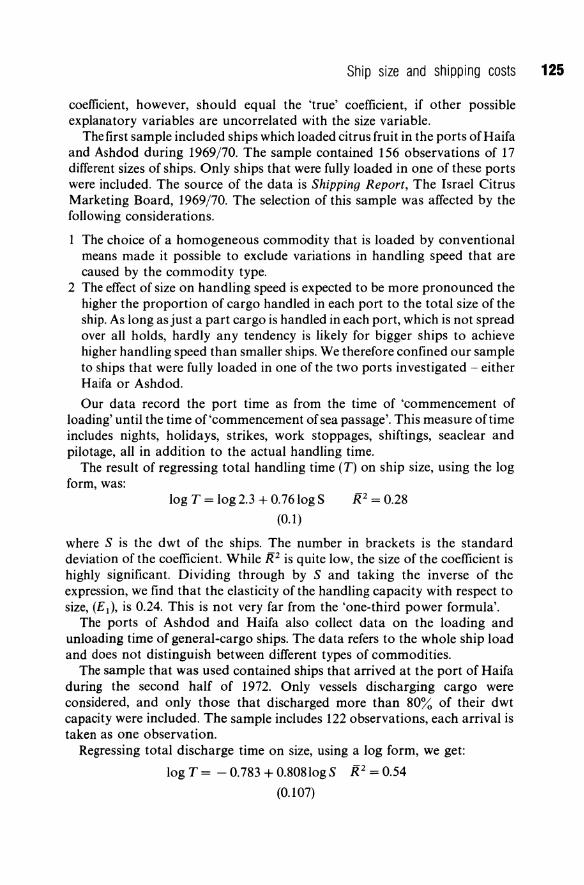
Ship size and shipping costs 125
coefficient, however, should equal the 'true' coefficient, if other possible explanatory variables are uncorrelated with the size variable.
The first sample included ships which loaded citrus fruit in the ports of Haifa and Ashdod during 1969/70. The sample contained 156 observations of 17 different sizes of ships. Only ships that were fully loaded in one of these ports were included. The source of the data is Shipping Report, The Israel Citrus Marketing Board, 1969/70. The selection of this sample was affected by the following considerations.
The choice of a homogeneous commodity that is loaded by conventional means made it possible to exclude variations in handling speed that are caused by the commodity type.
2 The effect of size on handling speed is expected to be more pronounced the higher the proportion of cargo handled in each port to the total size of the ship. As long as just a part cargo is handled in each port, which is not spread over all holds, hardly any tendency is likely for bigger ships to achieve higher handling speed than smaller ships. We therefore confined our sample to ships that were fully loaded in one of the two ports investigated - either Haifa or Ashdod.
Our data record the port time as from the time of 'commencement of loading' until the time of 'commencement of sea passage'. This measure oftime includes nights, holidays, strikes, work stoppages, shiftings, seaclear and pilotage, all in addition to the actual handling time.
The result of regressing total handling time (T) on ship size, using the log form, was:
log T = log2.3 + 0.7610gS
(0.1)
iF = 0.28
where S is the dwt of the ships. The number in brackets is the standard deviation of the coefficient. While iP is quite low, the size of the coefficient is highly significant. Dividing through by S and taking the inverse of the expression, we find that the elasticity of the handling capacity with respect to size, (Ed, is 0.24. This is not very far from the 'one-third power formula'.
The ports of Ashdod and Haifa also collect data on the loading and unloading time of general-cargo ships. The data refers to the whole ship load and does not distinguish between different types of commodities.
The sample that was used contained ships that arrived at the port of Haifa during the second half of 1972. Only vessels discharging cargo were considered, and only those that discharged more than 80% of their dwt capacity were included. The sample includes 122 observations, each arrival is taken as one observation.
Regressing total discharge time on size, using a log form, we get:
log T = - 0.783 + 0.80810g S iF = 0.54
(0.107)
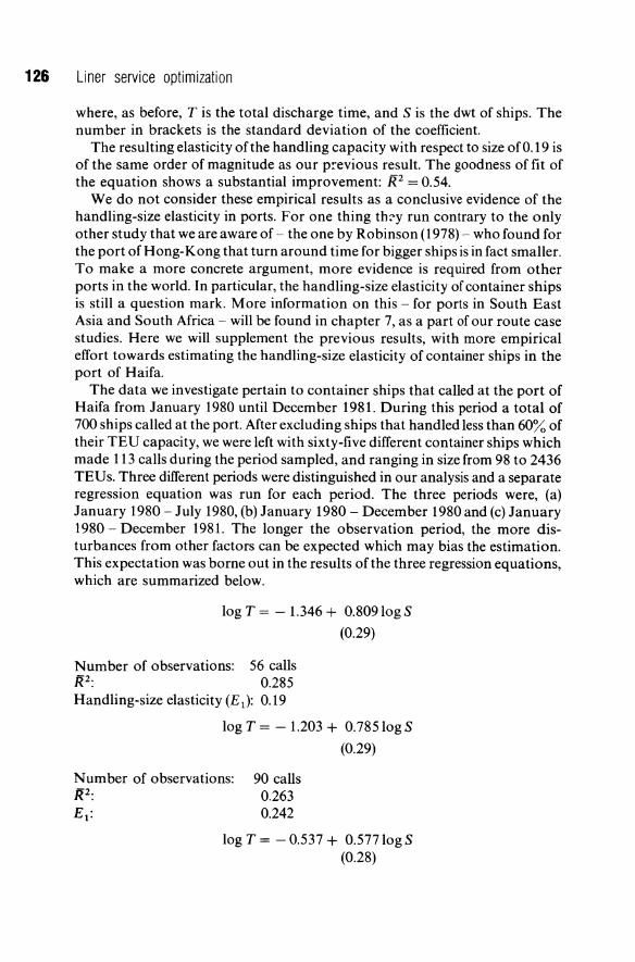
126 Liner service optimization
where, as before, T is the total discharge time, and S is the dwt of ships. The number in brackets is the standard deviation of the coefficient.
The resulting elasticity ofthe handling capacity with respect to size of 0.19 is of the same order of magnitude as our previous result. The goodness of fit of the equation shows a substantial improvement: jp = 0.54.
We do not consider these empirical results as a conclusive evidence of the handling-size elasticity in ports. For one thing th:-y run contrary to the only other study that we are aware of - the one by Robinson (1978) - who found for the port of Hong-Kong that turn around time for bigger ships is in fact smaller. To make a more concrete argument, more evidence is required from other ports in the world. In particular, the handling-size elasticity of container ships is still a question mark. More information on this - for ports in South East Asia and South Africa - will be found in chapter 7, as a part of our route case studies. Here we will supplement the previous results, with more empirical effort towards estimating the handling-size elasticity of container ships in the port of Haifa.
The data we investigate pertain to container ships that called at the port of Haifa from January 1980 until December 1981. During this period a total of 700 ships called at the port. After excluding ships that handled less than 60% of their TEU capacity, we were left with sixty-five different container ships which made 113 calls during the period sampled, and ranging in size from 98 to 2436 TEUs. Three different periods were distinguished in our analysis and a separate regression equation was run for each period. The three periods were, (a) January 1980 - July 1980, (b)January 1980 - December 1980 and (c) January 1980 - December 1981. The longer the observation period, the more disturbances from other factors can be expected which may bias the estimation. This expectation was borne out in the results of the three regression equations, which are summarized below.
log T = - 1.346 + 0.809 log S
(0.29)
Number of observations: 56 calls jP: 0.285 Handling-size elasticity (E 1): 0.l9
log T = - 1.203 + 0.785 log S
(0.29)
Number of observations: 90 calls 0.263 0.242
R2: E 1:
log T = - 0.537 + 0.577 log S (0.28)
Number of observations: iP: E 1 :
113 calls 0.183 0.423
Ship size and shipping costs 127
On the basis of these results it can be concluded that the results obtained for general-cargo ships by and large carryover to container ships. The handlingsize elasticity falls roughly in the same range as is expected for break-bulk ships. We have comparatively less confidence in the result of the third regression.
The proportion of variations explained by the equations, iF, is low for all three equations. This should be attributed to the large number of random influences that affect port operations - number of cranes available at the time ofloading, differences in the handling speed due to the exact berthing location of the ship, number of crew, strikes, and weather conditions. As long as the ship size provides a systematic explanation of the variations in the handling time, all these random variations can be assumed to be commensurate to this systematic component.
In our effort to find some general principles ofliner service optimization, we will make use of the relation HI = hISEl, where a lower limit for the value of El seems to be about 0.2 and a likely upper limit in the neighbourhood of the original value of 0.3 implied by Thorburn's principle. In specific case studies, where data are available, a separate estimate of this relation would be desirable.
5.5.2 The size elasticity of the hauling speed
A high design speed is very costly, both in terms of required horsepower and in terms of fuel consumption. However, to achieve a certain speed the required horsepower is less than proportional to ship size. This phenomenon is explained by the principle that the resistance ofthe water against the ship's hull does not increase at the same rate as the volume of the hull. The cost of the machinery per effect unit also declines. It pays to increase the design speed, as ships get bigger, also for this reason.
According to a time-honoured rule-of-thumb of naval architects, the design speed should increase by the square root of the length of the ship if the block coefficient and the Froude Number are held constant. In ship building this old rule-of-thumb is called the 'inch rule'. It implies that V = const st.
Our estimates of the size elasticity of the hauling speed adhere to the 'inch rule' so far as general-cargo ships are concerned. Three samples from this ship category were taken, and the regression of speed on ship size gave very similar results. As can be seen from Table 5.3, the three general-cargo ship size coefficients are almost identical and all are highly significant. Applying the same regression to tankers and bulk carriers produced different results.
The size elasticity of the hauling speed of tankers is close to zero. The size coefficient is significant at the 1 % level, and the equation (last row in Table 5.3)

128 Liner service optimization
Table 5.3 Results of regressing speed on size: log V = log canst + rx log S + log e
Number of Ship type observations log canst log S iP
General cargo ships' 50 1.3 0.16 0.42 (1.02)d (0.04)
General cargo shipsb 48 1.19 0.17 0.35 (1.01) (0.034)
General cargo shipsc 34 1.2 0.16 0.54 (0.026)
Dry bulk carriers' 50 2.59 0.013 0.015 (1.36) (0.01)
Tankers' 50 2.18 0.05 0.46 (0.08) (0.008)
·Source: World Ships on Order, February 1975. bSource: Shipping Statistics and Economics, H.P. Drewry (Shipping Consultants) Ltd. Various
issues, February-April, 1975. cA sample of ships of Zim Navigation Company taken in February 1976 by Nir Serlin. dFigures in parentheses are standard deviations of the coefficients.
explains 46% of the variations in the design speed. In the case of dry-bulk carriers, no significant relationships were found between the design speed and size.
We can summarize our findings by the following interval for values of the ship-size elasticity of the hauling capacity (= SV), where it seems that values applicable to general-cargo ships are to be found close to the upper limit, and values applicable to bulk-cargo ships (including tankers) are to be found close to the lower limit
where 1.00 < E2 < 1.17.
5.5.3 The size elasticities of the major factor costs
In the shipbuilding literature calculations of ship-size elasticities of various individual input requirements are common. From this source a complete list of ship-size elasticities of all major factor costs is, however, difficult to compile. Shipping economists - notably Thorburn (1960) - have studied the relationship between shipping costs and the size of ships of different types using a somewhat different breakdown of the costs than is usual in engineering-cost studies. The general pattern, if not exactly the size elasticities, of the
Ship size and shipping costs 129
dependence on ship size of the main accounting cost items - capital cost, operating costs (or 'day costs'), and bunker cost - is fairly well documented in the shipping-economics literature. We have contributed some further empirical evidence of the size elasticities of these costs. A disadvantage of adhering to the rather aggregated accounting cost categories is that the real sources of the observed economies of ship size will remain hidden to some extent. In the following discussion we have tried to go into more detail in some respects by drawing on the results of some marine-engineering studies, too.
(a) Capital costs of ship and cargo
The capital cost of the ship and the cargo aboard the ship per day can most adequately be regarded as an opportunity cost. An alternative use of the ship which may be interesting for the owner is, for example, to charter out the ship. In this case the ruling-time charter rate is the ship's capital cost. In another case the best alternative use can be to employ the ship in another liner trade. The net earnings per day foregone by not seizing this opportunity is the ship's capital cost in that case.
The point is in the present connection that at the time when the ship was ordered, the expected total capital cost defined as above, will under competitive conditions coincide on average with the cost of building the ship. The following discussion is therefore concerned with the relationship between the shipbuilding cost and the ship size.
The opportunity cost of the cargo aboard the ship is traditionally calculated as the cost of interest of the goods making up the cargo. Either the exporter or the importer of the goods will suffer a delay in sales revenue corresponding to the time oftransit. This view ofthe transit-time cost of the cargo will do well for the present purpose. In chapter 7 a more penetrating discussion of this matter is presented. Note also that this cost is indirectly borne by the shipowner. The wareowners' interest costs will be reflected in the freight rates that they are prepared to bear. The ship-size elasticity of the interest cost of the cargo is obviously unity, since the ship size is defined as the holding capacity of the ship. The size elasticity of the building cost of the ship is a considerably more involved matter.
The most well-known geometric principle with a bearing to shipbuilding cost is the 'two-thirds power rule'. The holding capacity of any container is equal to the volume, whereas the construction cost tends to be proportional to the surface area of the container, no matter whether it is box-shaped, ballshaped or has the form of a ship's hull. There are, however, many more aspects to the matter of the relationship between ship capital cost and ship size.
The main components of capital costs are, (a) the hull costs, and (b) the cost of the propulsion machinery. The former is about two to three times (in the case oflarge bulk carriers and tankers) the latter. The hull cost is traditionally divided into hull engineering, outfit, and steelwork, of which the latter can

130 Liner service optimization
make up almost one-halfthe total hull cost, although it varies with the price of steel.
The least-important source of the economies of size is, in fact, steel requirement. It is true that the area of the enclosed space varies approximately as the two-third power of ship size. This potential sa ving is, however, offset to a large degree by the need for thicker steel plate as ships get bigger. On the other hand, savings in shipyard cost of labour of erecting the hull structure are possible, as larger elemental pieces of metal are used and larger subassemblies employed for bigger ships.
Engineering studies of shipbuilding economies of ship size indicate that it is the labour input, rather than the input of material, that decreases per ton of dwt as ships get bigger. Erichsen (1971) quotes a number of studies giving formulae for the labour and material costs of hull engineering, outfit, and steel structures that imply that the size elasticities of the labour inputs are in the 0.6-0.7 range, whereas the size elasticities of material requirements exceed 0.8 and even, in the case of the steel structures of container ships, 0.9.
To attain a certain speed, the horsepower requirement of the machinery is less than proportional to ship size. This advantage of size is often traded off against higher speed; but as the construction cost of the machinery per effect unit seems to decrease in a wide range, the cost of machinery contributes to the size economies in capital costs, even if installed horsepower is commensurate with the size of the ship.
This can be exemplified by means of the shipbuilding rule-of-thumb that makes horsepower (HP) proportional to the two-third power of the displace-
2
ment, multiplied by the cube of the design speed; i.e. HP = const S3 V 3 • Given the speed, it is clear that substantial savings in horsepower per dwt ton can be realized. Only a minute increase in speed will, however, easily offset this saving. According to Chapman (1969) the elasticity of the capital cost of a dieselengine plant with respect to the brake horsepower equals 0.614. As for steam turbine plants, Benford (1968) gives a formula in which the capital cost is proportional to the shaft horsepower raised to the power of 0.6.
The results of our empirical analysis suggest that the sum of all the various economies of ship size in shipbuilding cost happens on balance to adhere to the 'two-thirds power rule'.
Our sample consisted of fifty observations of the contracted prices of bulk carriers taken from various issues of Drewry. Only ships that were due for delivery in 1976/77 were included, so that inflation was neutralized. Regressing the costs of new building on the size of the ship, using an exponential form of the regression equation,
log (building cost) = - 4.236 + 0.655 log S iP = 0.34
(0.818) (0.088)
where S is the deadweight tonnage ofthe ship The results clearly conform with the 'two-thirds power rule' but there cannot be a single rationale for this. The
Ship size and shipping costs 131
result should be interpreted in this way. There are more or less marked economies of ship size in the costs of machinery, hull engineering, outfit, steelwork etc., and as a whole it seems that the ship capital cost is proportional to the two-thirds power of the ship size. This result has been confirmed by a number of other studies (see the summary below).
(b) Operating cost
Within the aggregate of operating cost, mutually counteractive forces are concealed. So far as the development of costs with increases in ship size is concerned, the single, most important source of size economies are crew wages. The manning requirement is determined by a fairly fixed number of ' tasks'. The extent of each task will increase much more slowly than in proportion to ship size. This is the same principle, basically, as that exemplified by the simple fact that 'there is no need for more than one driver, however big the car'. Automation in shipping will eventually make crew wages a fixed cost with respect to ship size. Goss and Jones (1971) fix the crew size of dry-bulk carriers at thirty-eight men for all ships bigger than 25000 dwt (the biggest is 200000 dwt). Due to automation and reorganization of the functions of the crew, newly built large bulk ships, container ships and tankers have crews of eighteen to twenty-one men. Erichsen (1971; p.192) gives the elasticities of the crew cost with respect to size as 0.10 for container ships and 0.03 for tankers, claiming that these values are applicable to ships 'having a level of automation which is practical today'.
Crew cost is counterbalanced by maintenance and repair costs and insurance, which together are of an order of magnitude comparable with the crew cost. For smaller ships, crew cost is normally the larger item, but it is the smaller item for bigger ships. The size elasticity of maintenance and repair cost is roughly the same as that of the total capital cost. The size elasticity of insurance is higher for very large ships than for ships of moderate size. Erichsen has calculated this size elasticity as 0.7 for container ships and 1.25 for tankers exceeding 100000 dwt.
Our empirical analysis of crew costs is based on data of thirty-four ships of Zim Navigation Company. Information on costs was taken from the company's accounts. The regression result is summarized below:
log (crew cost) = log 12.8 + 0.03 logS (0.10)
R2 =0.003.
The size elasticity of the crew cost is very small (close to zero) as predicted. The size coefficient, however, is certainly not significant and the proportion of variations explained by the equation is trivially small. Our results, therefore, did not point at any significant relationships between size and crew costs.
We have also explored the relationships between all operating costs (except fuel) and ship size on the same sample. The result was:
132 Liner service optimization
log (operating cost) = log 10.5 + 0.43 log S (0.09)
iP = 0.41.
The explanatory power of the equation is now much greater, and the size coefficient is highly significant. The ship-size elasticity, 0.43 adheres closely to the result of other studies (see below).
( c) Fuel cost
In every marine engineering study that we have consulted, fuel consumption and installed horsepower are assumed to be proportional. Economies of ship size in the fuel consumption can therefore be expected to be enjoyed on account of the fact that for a given design speed the horsepower requirement is somewhat less than proportional to ship size.
This effect can be difficult to isolate as, so far as general-cargo ships are concerned, the design speed is normally not constant with respect to ship size. Normally the observed relationship between fuel consumption and ship size would reveal the total size elasticity of fuel consumption.
We have estimated the partial elasticity of the fuel consumption with respect to ship size by selecting a sample of ships of different sizes of Zim Navigation Company in which the variations in design speed are minute. We have regressed the fuel costs recorded in 1976 on ship size, with the following result:
log(fuel cost) = log 6.25 + O.72logS iP = 0.74.
(0.07)
( d) Port charges on the ship
The most important charges payable by shipping lines in port are the stevedoring charges. These are assigned to the cargo costs.
The port charges intended to recoup the port authorities' cost of berthing facilities, cranes etc., from the shipowners are in total many times less than the stevedoring charges. These port charges are levied partly on the cargo loaded/unloaded by the ships, and partly on the ships themselves in one way or the other. The former category of port charges can obviously be referred to the cargo costs. The latter category of port charges can be further divided into, (a) time-proportional berth occupancy charges, and (b) charges on the ship which are independent of the lay time of the ship.
Concerning group (a) the question is, how the charge per unit of time is differentiated between different ships? In a large majority of cases some measure of ship size - most often the net registered tonnage (see Table 5.4) - is the basis of differentiation. In this majority case the size elasticity of the port charges on the ships can be taken to be unity. If the berth occupancy charges are differentiated according to the length of ships which is the case in some ports, the size elasticity of these charges is as low as one-third.

Ship size and shipping costs 133
Table 5.4 Percentage distribution of cases where port charges on ships were based on
Length Draft N arne of charges GRT NRT of ship of ship
Port time due on ship 21 68 5 Aids to navigation 8 82 Pilotage 28 38 17 Towage 38 12 Berthing/unberthing 25 20 5 Berth occupancy 18 42 30
Source: Port Pricing; Report by the UNCT AD Secretariat, TD/B/C. 4/110, United Nations, New York, 1973.
Other"
6 100 100 100 100 tOO tOO
"The 'other' basis includes flat charges per operation, and, for example, per hour of tug use for towage.
The UNCT AD secretariat has made a survey of the port-charging practices in over 100 ports of the world. Table 5.4 summarizes the findings of the survey as regards the bases of differentiation of both time-dependent and timeindependent port charges. In a majority of cases the berth occupancy charges were time proportional.
The time-independent port charges on the ship are typically paid for specific services like aid to navigation and towage, but can also be imposed on very general grounds; the so-called 'port dues on the ship' in the UNCT AD survey were found to be time-independent in more than half the cases.
The bases for differentiation between ships of the time-independent port charges vary a great deal from one port to another. One common basis of differentiation is, as in the case of time-proportional charges, the GRT or another measure of ship size. In that case the charge can be referred to the cargo costs, because, on the assumption that the total cargo and the ship size are proportional, time-independent charges of the ship, which are differentiated according to ship size will, in effect, be proportional to the tons of cargo handled.
Normally, however, there is a final pot ofleft-overs - port charges which can be assigned neither to the time-proportional costs nor to the cargo costs. These charges can be time-independent flat charges (i.e. invariate ofthe type or size of ships), or time-independent charges, which increase less than in proportion to the ship size.
These 'left-overs', which will be referred to as flat port charges, are so relatively insignificant that they could very well be disregarded in the model. However, there is another analytical problem associated with the model, which so far has not been mentioned, which, as a matter offact, becomes easier to handle if the flat port charges are taken into account.

134 Liner service optimization
( e) Time-independent, flat port charges and transitory time
So far we have implicitly assumed that the time of service of a ship per year is spent either in handling or in hauling operations. This may seem to neglect so called 'transitory time'. Port time typically includes a fixed (but subject to random variations) portion and a portion which is approximately proportional to actual cargo-handling time. The fixed port time is here called transitory time, because it occurs between the time of the start or the end of handling activities and the time of proper hauling activities. (The fact that handling operations do not go on 'round the clock' does not matter as long as the time of stoppages etc., is proportional to effective cargo handling time in the same way as nights are proportional to work days.)
The models would become less handy if a third item of the service time of ships were to be included. A 'trick' which avoids this complication without doing much harm to the realism of the model, is to refer transitory time to atsea time. All costs incurred at sea except fuel costs are also incurred during the transitory time in port. By the following procedure this inaccuracy will be eliminated to some extent.
The model would likewise be less handy if costs were not time-proportional or proportional to tons handled, like the cargo costs. The flat port charges which have been left over, constitute such an irregular item. However, by assuming that the flat charges for pilotage, towage, etc. are incurred during transitory time, the cost per hour of transitory time becomes close to the cost per hour of progress-at-sea time.
Therefore, by simply adding to the distance, D, an increment that - in miles - corresponds to the duration of transitory time, we get rid of two problems at a very small cost in terms of reduced precision. The time at sea on each leg is thus to be regarded as the time from stowing the last ton of cargo in the port ofloading to the placing on the quay of the first ton of cargo in the port of discharge.
( f) Summary of the analysis of the size elasticities of the factor costs
Our findings as to the ship-size elasticities of the time-proportional costs are summarized in Table 5.5. There some comparable results of four other representative studies are included.
As can be seen the general agreement is quite striking so far as the capital and operating costs are concerned, even between different ship types. The lowest size elasticity is in all cases exhibited by the operating costs, and ship capital cost comes in second place.
Our estimate of the partial size elasticity of the fuel cost is consistent with the findings as to dry bulk carriers and tankers of Goss and Jones (1971) and Heaver (1968), but deviates a great deal from Thorburn's (1960) result. The explanation is that dry-bulk carriers and tankers show very small increases, or

Ship size and shipping costs 135
Table 5.5 Ship size elasticities of capital cost, operating cost, and fuel cost
Capital cost
Ship type
Tramps (Thorburn) 0.67
Liner (Getz et al.) 0.6
Dry bulk carrier (Goss and Jones) 0.7
Tanker (Heaver) 0.6
Authors' estimate (regression results) 0.6
Operating cost (except fuel)
0.4
0.6
0.4
0.3
0.4
Fuel cost (for propulsion)
1.00
0.8
0.6
0.72
no increase at all, as we have found in the case of tankers, in design speed with increases in ship size. The considerably higher size elasticity given by Thorburn (1960) is not a partial elasticity, and the design speeds of the ships in his sample were increasing with growing ship size according to the inch rule, which works to raise the total size elasticity of the fuel cost quite substantially.
The wide span of the size elasticities of the berth occupancy charges given in the bottom row gives an exaggerated impression of great variations. In most cases unity is the applicable value. However, it is reported that some ports differentiate the occupancy charges according to ship length rather than according to ship size.
5.6 ECONOMIES OF SIZE AT SEA - DISECONOMIES OF SIZE IN PORT
We have now the required information about shipping costs and ship size for fulfillment of one main purpose of this chapter - the demonstration that economies of ship size are enjoyed at sea, while diseconomies of ship size are suffered in port and that the choice of optimal ship size involves a balancing of the cost per ton at sea and the cost per ton in port.
By applying the estimated size elasticities, ei,ej'£l and E2 to the total cost per ton of equation (5.1), the following conclusions can be drawn.
The difference ej - E2 is negative for all cost items. This is a result of our finding that £2 is greater than 1, while the values of ej range from about 0.4 to 1.0. The total hauling cost per ton, consequently, decreases as ship size increases.

136 Liner service optimization
2 The difference ei - E 1 is positive for all cost items. This is a result of our finding that E 1 is in the 0.2-0.3 range, while the values of ei are in no case less than 0.3. Since cargo costs are invariant to ship size, it is clear that the total handling cost per ton increases with ship size.
We are in a position now to compare the nature of economies of 'plant size' in shipping with that in industry in general.While plant size can unequivocally be defined as plant-output capacity, ship size is certainly not synonymous with the capacity of shipping services. Ship size equals only to holding capacity. It is instead the handling and the hauling capacities which correspond to the plant output capacity. The elasticities of total capital cost and total operating cost will, therefore, be calculated with respect to HI and H 2, and a comparison will be made with the previously cited elasticity values derived by Haldi and Whitcomb (1967). The H I-elasticity of the ith factor cost is given by the ratio e 1/ E 1 and the H 2-elasticity of the jth factor cost is given by the ratio ej /E 2 •
From the discussion ofthe previous section it follows that a size elasticity of the capital cost of 0.6 and a size elasticity of the operating cost of 0.4 are representative. The size elasticities of the handling capacity, E l' can be assumed to be in the 0.2-0.3 range, and the size elasticity of the hauling capacity, E2 ranges from 1.17 down to unity.
Recalling that Haldi & Whitcomb (1967) have found that the capital-cost elasticity with respect to industrial plant capacity is concentrated in the 0.6-0.8 range, and that the labour cost elasticity with respect to industrial plant capacity is normally less than 0.4, it is striking how typically ship capital and operating costs develop with respect to the hauling capacity, H 2' in the range of 0.57-0.67 and 0.34-0.4 respectively and how atypically these costs develop with respect to the handling capacity, HI' 2-3.33 and 0.2-2 respectively.
It should be mentioned that crew costs, rather than operating costs, would be more comparable to the labour costs calculated by Haldi and Whitcomb (1967). The elasticity of crew costs are still lower than that of ship-operating costs. As for fuel costs, Haldi and Whitcomb (1967; p. 192) concluded that 'unit costs for utilities (fuel, electric power, etc.) sometimes decline slightly with size increases, because larger furnaces, motors and other such equipment units perform more efficiently than smaller ones'. This assessment also agrees well with our findings regarding the elasticity offuel cost with respect to the hauling capacity.
5.6.1 Some reflections about the economies and diseconomies of size in port of bulk carriers and tankers
The key aspect of our model of ship-size optimization is that the size elasticity of the handling capacity, E 1 , is comparatively low, lower, in particular, than all values of ei.

Ship size and shipping costs 137
The authors' estimates of the value of E 1 apply to conventional generalcargo liners and tramps. We have no evidence of the value of E1 for bulk carriers and tankers. Can it be assumed that diseconomies of size in port are a valid proposition also for these ship categories?
Some authorities contend that a size elasticity of 0.3 is too low for bulk carriers and tankers. Goss (1970), in a study of bulk carriers, goes as far as saying that 'at the moment I do not think we can even say that most big ships take longer to turn round than most of the smaller ones; for big ships often get the better berths, while small ships may be relegated to the older ones'.
An implicit premise of the theory that handling capacity is proportional to length is that each hold is worked at a constant speed irrespective of ship size. It is only by variations in the number of holds that ships of different size exhibit different overall handling speeds. This premise may be qualified on two counts. Two forces - working in opposite directions on handling capacity - should be mentioned.
First, as each hold is wider and deeper the bigger the ship is, the crane cycle will be longer the bigger the ship is. This would tend to reduce the handling speed per crane. On the other hand, the incentive to improve the handling performance will be greater, the greater the potential cost savings are. The question is how strong this incentive is in different cases, and how costly it is to improve handling performances. Goss and Jones (1971) observe in discussing the economies of size in bulk carriers that 'it is worthwhile providing better equipment on the berths they are to use, and this seems to be supported by the experience of tanker owners, who install more powerful pumps in the larger ships, so that their loading and discharging rates may be roughly proportionate to their size, and their turn round times much the same as the smaller ships'.
The implications of these points may be elucidated by considering the expression for C 1 (the indirect handling cost per ton, i.e. total handling costs per ton minus direct stevedoring charges)
The first point, that the biggest ships get the best berths, would ceteris paribus raise E 1 above the value of 0.3 predicted by the theory of lengthproportional handling capacity. It would, however, not leave all other elasticities in the expression for C 1 unaffected.
It is unlikely that the big ships receive higher-quality port service for nothing. It should be reflected in the port dues - in 'cranage' in particular -which would raise the value of ei pertaining to port charges in the expression above.
The second point, that the ships themselves tend to be equipped such, or
138 Liner service optimization
constructed in a way, that offset the basic loading and unloading diseconomies of size, should also be reflected in the value of e i , besides the value of E 1. The size elasticity ofthe capital cost should go up together with the size elasticity of handling capacity.
The handling operation does present the greatest problem for research into optimal ship design for the simple reason that ports around the world are so very different. The hauling operations of ships do not depend very much on exogenous circumstances but this is certainly not so with regard to operations in port. Many, therefore, felt understandably reluctant to go very deep into the dependence of the handling capacity on ship size. 'I doubt whether any general relationship· .. can be specified and certainly not in a simple way. The area could perhaps be explored by the use of multiple regression analysis, but systematic data on ship turnround is not published··· ' (Goss 1970).
Something has to be assumed about port time, however, in order to produce a complete cost estimation. The almost unanimous choice seems to have been to assume turnround time to be constant, i.e. independent of ship size. This assumption implies that there are significant economies of size also in the handling operation. This implication does not seem to be fully appreciated; constant port time is supposedly considered to be the most 'neutral' assumption. Constant port time means that the handling cost per ton is falling as ship size is increasing because ei - E 1 is negative for all i.
An alternative, equally simple, and more realistic provisional convention would be to assume the indirect handling cost rather than the time in port to be constant. This would mean that the weighted average of ei - E1 is assumed to be equal to zero. In the absence of systematic data for handling speeds of tankers and dry-bulk carriers this seems to be a preferable assumption to base a cost model on.
A great deal of research is required to establish the relationship between handling capacity and ship size. It would be very interesting to examine if cargo-handling productivity improvement have been 'size-biased' to such an extent for tankers and bulk carriers that the point is reached where diseconomies of size in port no longer apply. Finally, it should be pointed out that port charging practices play the role of 'the joker' in this game. To some extent it is up to the port authority whether port diseconomies of ship size will be realized or not by the shipowner.
5.7 OPTIMAL SHIP SIZE
The optimal ship size is obtained by trading off economies of size in the hauling operations with diseconomies of size in the handling operations. The model can be given the standard engineering cost balancing form shown in Fig. 5.1.
The optimum ship size is found at the point where the slope ofthe handling-
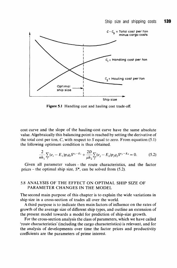
I Optimal I Shipsize~
I
Ship size and shipping costs 139
C - C3 = Total cost per ton minus cargo costs
C1 : Handling cost per ton
Cz: Hauling cost per ton
Ship size
Figure 5.1 Handling cost and hauling cost trade-ofT.
cost curve and the slope of the hauling-cost curve have the same absolute value. Algebraically this balancing point is reached by setting the derivative of the total cost per ton, C, with respect to S equal to zero. From equation (5.1) the following optimum condition is thus obtained.
Given all parameter values - the route characteristics, and the factor prices - the optimal ship size, S*, can be solved from (5.2).
5.8 ANALYSIS OF THE EFFECT ON OPTIMAL SHIP SIZE OF PARAMETER CHANGES IN THE MODEL
The second main purpose of this chapter is to explain the wide variations in ship size in a cross-section of trades all over the world.
A third purpose is to indicate then main factors of influence on the rates of growth of the average size of different ship types, and outline an extension of the present model towards a model for prediction of ship-size growth.
For the cross-section analysis the class of parameters, which we have called 'route characteristics' (including the cargo characteristics) is relevant, and for the analysis of developments over time the factor prices and productivity coefficients are the parameters of prime interest.
140 Liner service optimization
5.S.1 Cargo and route characteristics and optimal ship size
The route characteristics included in the model are: the directional cargo balance, p,; the average handleability of cargo and/or the port productivity, which are both incorporated in hI; the number of work hours per day in port, n.
The effect of a change in the route characteristics on the optimal ship size is shown by calculating the partial derivative of optimal ship size (S*) from equation (5.2) with respect to D, p" n, and hI. On the basis of our results that ei - El is positive and ej - E2 is negative, for every i andj, the following signs of the partial derivatives can easily be shown to apply.
Positive derivatives
Negative derivatives
as* ->0 aD
as* ah 1 > 0,
as* an >0.
as* ap, <0.
Distance, as expected, has a positive effect on ship size, which can be explained in diagrammatical terms by the aid of Fig. 5.1. An increase in D shifts the C 2-
curve proportionately upwards. The slope ofthe C2-curve, therefore, becomes steeper, and the point of the minimum of the C-curve will move to the right in the direction of increasing the ship size.
An increase in the average handleability of cargo, or the level of port productivity per hour, and an increase in the total number of hours of work per day in port will have the same positive effect on ship size. Diagrammatically, an increase in hi or n will shift the C I-curve proportionately downwards so that its slope becomes flatter, which will move the minimum point of the Ccurve to the right.
The cargo balance in the trade is a factor which plays a perhaps somewhat unexpected role for the optimal ship size. The more balanced the route is the smaller the optimal ship size tends to be. An increase in p, will shift the C2-curve downwards so that its slope becomes flatter, which will move the minimum point of the C-curve to the left. In Part III we will return to the issue of optimal ship size and the cargo balance. We will show that in an unbalanced trade, there are two optimal ship sizes: one larger size of ships, which load cargo only in the fat direction and sail in ballast on the meagre leg, and another smaller size of ships, which sail fully loaded on both legs. However, it will be shown that this division of labour will be realized only provided that the levels of freight rates in the two directions are disparate in accordance with the disparate levels of the marginal costs of shipping. As this proviso is not fulfilled
Ship size and shipping costs 141
in liner trades, the two optimal sizes in one and the same trade cannot be observed in reality.
The degree of cargo imbalance is a very interesting aspect in the present connection although it cannot be claimed to be of central importance for the general issue of optimal ship size.
The relative strength of the partial effects of the different route characteristics on optimal ship size can be measured by the respective partial elasticities. It is easily shown that the absolute values of the partial elasticity of S* with respect to each of D, jl, hi and n are all identical.
(~~)(~ )=( _ a~*)(:* )=(~!~)(~~ )=(a!*)(s: )=e. The value of e depends first on the values of the size elasticities ei,ej,E i
and E 2, and second on the factor proportions in the handling and hauling operations, respectively. The former set of values are inherently fixed to a high degree, while the latter set of values show some variations between different trades, in particular between short-sea and deep-sea trades. The variations are, however, not more important than that e seems to be confined to a rather narrow band of values from about 1.00 to 1.25 in the great majority of realistic cases.
The two route characteristics which exhibit by far the widest span of variations are the route distance, D, and the handleability of cargo, expressed in hi' The cargo balance varies only between 1 (representing a trade where zero cargo moves on the meagre leg) and 2 (representing a perfectly balanced trade), and the relative variations are of a similar order of magnitude.
In view of this and the aforementioned fact that the absolute values of partial elasticities of S* with respect to all route characteristics are the same, it is clear that the greatest differences in ship size are to be found between shortsea and deep-sea trades, on one hand, and between trades in different commodities, on the other.
These two aspects - the ship-size distribution with respect to route distance, and the ship-size distribution with respect to cargo handleability - are worthy of a fuller discussion.
( a) Ship size distribution with respect to cargo handleability
In the past the quickest 'loading and unloading' by far was achieved by ships for passengers. Therefore long-distance passenger liners used to be the largest ships on the seas, at least in terms ofGRT. Liquids, like crude oil, are the most easily handled freight, provided that the carrier is built as a tanker. The handling speed attained by some dry-bulk carriers is, however, not much behind that of oil tankers. The giant ships of today are consequently oil tankers and, second, dry-bulk carriers. The reason for the wide span of ship sizes on a given trade route, from conventional general-cargo liners at one end
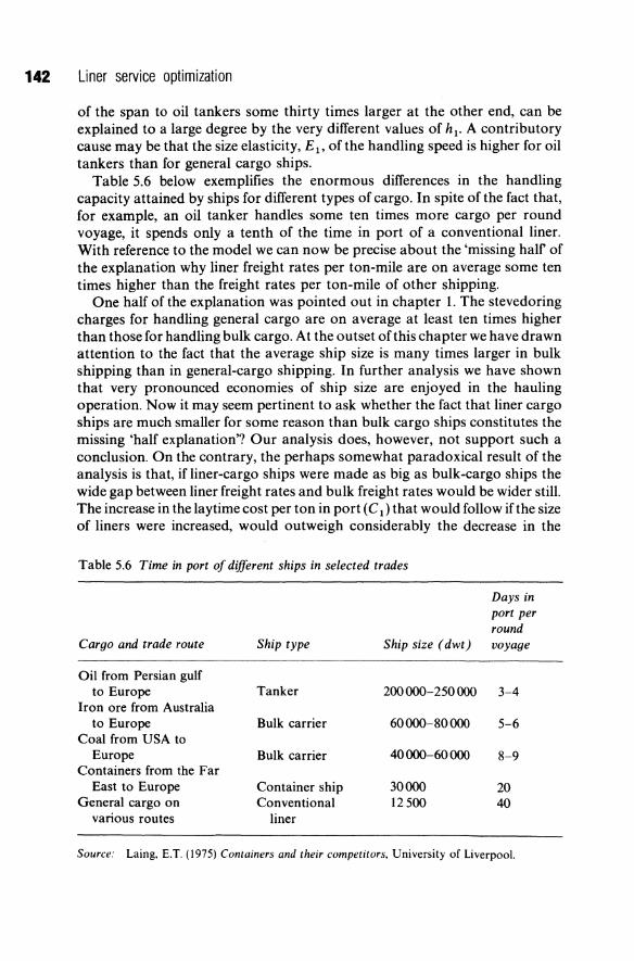
142 Liner service optimization
of the span to oil tankers some thirty times larger at the other end, can be explained to a large degree by the very different values of hI' A contributory cause may be that the size elasticity, E 1 , of the handling speed is higher for oil tankers than for general cargo ships.
Table 5.6 below exemplifies the enormous differences in the handling capacity attained by ships for different types of cargo. In spite of the fact that, for example, an oil tanker handles some ten times more cargo per round voyage, it spends only a tenth of the time in port of a conventional liner. With reference to the model we can now be precise about the 'missing half of the explanation why liner freight rates per ton-mile are on average some ten times higher than the freight rates per ton-mile of other shipping.
One half of the explanation was pointed out in chapter 1. The stevedoring charges for handling general cargo are on average at least ten times higher than those for handling bulk cargo. At the outset of this chapter we have drawn attention to the fact that the average ship size is many times larger in bulk shipping than in general-cargo shipping. In further analysis we have shown that very pronounced economies of ship size are enjoyed in the hauling operation. Now it may seem pertinent to ask whether the fact that liner cargo ships are much smaller for some reason than bulk cargo ships constitutes the missing 'half explanation'? Our analysis does, however, not support such a conclusion. On the contrary, the perhaps somewhat paradoxical result of the analysis is that, if liner-cargo ships were made as big as bulk-cargo ships the wide gap between liner freight rates and bulk freight rates would be wider still. The increase in the lay time cost per ton in port (C 1) that would follow if the size of liners were increased, would outweigh considerably the decrease in the
Table 5.6 Time in port of different ships in selected trades
Days in port per round
Cargo and trade route Ship type Ship size (dwt) voyage
Oil from Persian gulf to Europe Tanker 200000-250000 3-4
Iron ore from Australia to Europe Bulk carrier 60000-80000 5-6
Coal from USA to Europe Bulk carrier 40 000-60 000 8-9
Containers from the Far East to Europe Container ship 30000 20
General cargo on Conventional 12500 40 various routes liner
Source: Laing, E.T. (1975) Containers and their competitors, University of Liverpool.
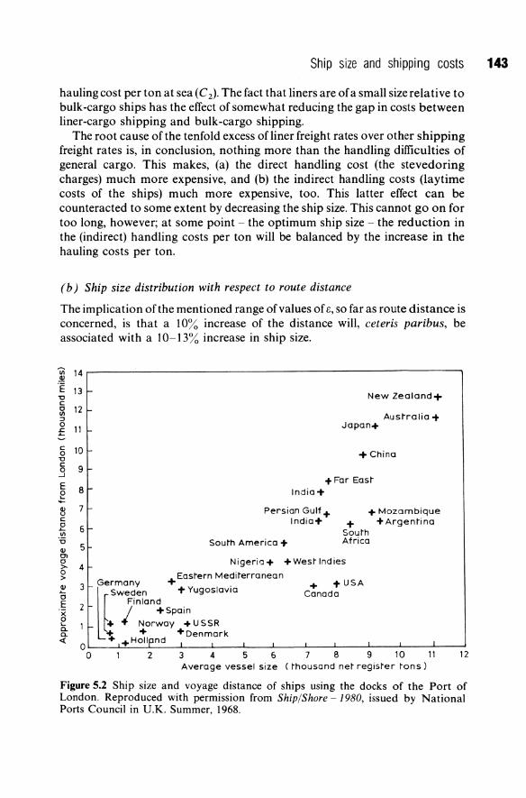
Ship size and shipping costs 143
hauling cost per ton at sea (C 2 ). The fact that liners are ofa small size relative to bulk-cargo ships has the effect of somewhat reducing the gap in costs between liner-cargo shipping and bulk-cargo shipping.
The root cause of the tenfold excess of liner freight rates over other shipping freight rates is, in conclusion, nothing more than the handling difficulties of general cargo. This makes, (a) the direct handling cost (the stevedoring charges) much more expensive, and (b) the indirect handling costs (lay time costs of the ships) much more expensive, too. This latter effect can be counteracted to some extent by decreasing the ship size. This cannot go on for too long, however; at some point - the optimum ship size - the reduction in the (indirect) handling costs per ton will be balanced by the increase in the hauling costs per ton.
(b) Ship size distribution with respect to route distance
The implication of the mentioned range of values of 1::, so far as route distance is concerned, is that a 10% increase of the distance will, ceteris paribus, be associated with a 10-13% increase in ship size.
VI 14 ~ °E 13 f-1:> C 0 12 e-I/) ~ 0
11 ~ ..... c 10 0
1:> C
9 0 ....J
E 8 0 L. .... II! 7 u c 0 6 .L. I/)
0-6 II! 5 01 0 >- 4 0 > II! 3 (; E 2 >( 0 L-a. a. <{
0 0
New Zealand+
Aus~ralia -t Japan+
+ China
+ Far Eas~ India+
Persian Gulf + + Mozambique India+ + +Argen~ina
Sou~h Sou~h America + Africa
Nigeria+ +Wes~ Indies
+ Eas~ern Medi~erranean Germany
~ Sweden + Yugoslavia l Finland I +Spain
+ Norway +USSR ~ + +Denmark
+Hollpnd
1 2 3 4 5 6
+ + USA Canada
7 8 9 10 Average vessel size (rhousand ner regis~er ~ons)
11 12
Figure 5.2 Ship size and voyage distance of ships using the docks of the Port of London. Reproduced with permission from Ship/Shore - 1980, issued by National Ports Council in U.K. Summer, 1968.
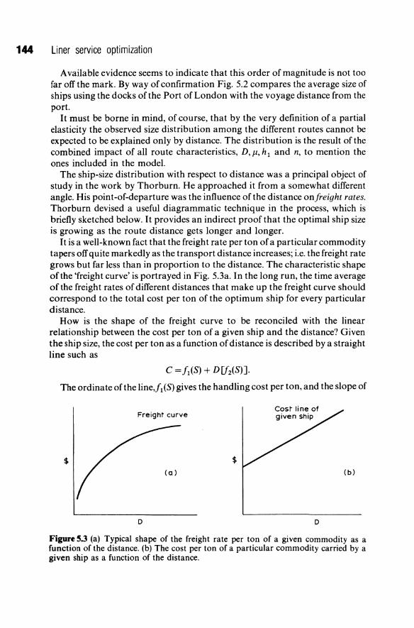
144 Liner service optimization
A vailable evidence seems to indicate that this order of magnitude is not too far off the mark. By way of confirmation Fig. 5.2 compares the average size of ships using the docks of the Port of London with the voyage distance from the port.
It must be borne in mind, of course, that by the very definition of a partial elasticity the observed size distribution among the different routes cannot be expected to be explained only by distance. The distribution is the result of the combined impact of all route characteristics, D, 11, hl and n, to mention the ones included in the model.
The ship-size distribution with respect to distance was a principal object of study in the work by Thorburn. He approached it from a somewhat different angle. His point-of-departure was the influence of the distance onfreight rates. Thorburn devised a useful diagrammatic technique in the process, which is briefly sketched below. It provides an indirect proof that the optimal ship size is growing as the route distance gets longer and longer.
It is a well-known fact that the freight rate per ton of a particular commodity tapers off quite markedly as the transport distance increases; i.e. the freight rate grows but far less than in proportion to the distance. The characteristic shape ofthe 'freight curve' is portrayed in Fig. S.3a. In the long run, the time average of the freight rates of different distances that make up the freight curve should correspond to the total cost per ton of the optimum ship for every particular distance.
How is the shape of the freight curve to be reconciled with the linear relationship between the cost per ton of a given ship and the distance? Given the ship size, the cost per ton as a function of distance is described by a straight line such as
C = fl(S) + D[f2(S)].
The ordinate of the line'!l (S) gives the handling cost per ton, and the slope of
Freight curve
$ $
D
Cos~ line of given ship
D
(b)
Figure 5.3 (a) Typical shape of the freight rate per ton of a given commodity as a function of the distance. (b) The cost per ton of a particular commodity carried by a given ship as a function of the distance.
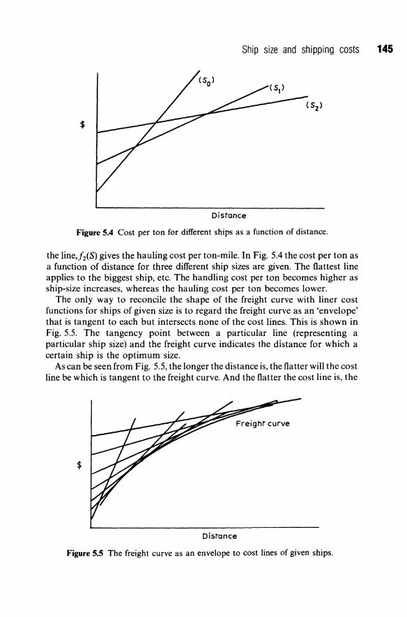
Ship size and shipping costs 145
$
Distance
Figure 5.4 Cost per ton for different ships as a function of distance.
the line,j2(S) gives the hauling cost per ton-mile. In Fig. 5.4 the cost per ton as a function of distance for three different ship sizes are given. The flattest line applies to the biggest ship, etc. The handling cost per ton becomes higher as ship-size increases, whereas the hauling cost per ton becomes lower.
The only way to reconcile the shape of the freight curve with liner cost functions for ships of given size is to regard the freight curve as an 'envelope' that is tangent to each but intersects none of the cost lines. This is shown in Fig. 5.5. The tangency point between a particular line (representing a particular ship size) and the freight curve indicates the distance for which a certain ship is the optimum size.
As can be seen from Fig. 5.5, the longer the distance is, the flatter will the cost line be which is tangent to the freight curve. And the flatter the cost line is, the
Freight curve
$
Distance
Figure 5.5 The freight curve as an envelope to cost lines of given ships.
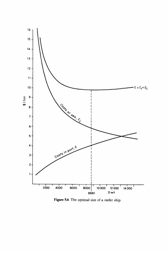
16
15
14
13
12
11
10 C=C1+C2
c: 0
9 ......
~
8
7
6
5
4
3
2
2000 4000 6000 BOOO 10000 12 000 14000
8881 Dwt
Figure 5.6 The optimal size of a reefer ship.

Ship size and shipping costs 147
bigger is the applicable ship. Hence, the longer the distance is, the bigger the optimal ship size will be.
5.9 THE OPTIMAL SIZE OF A PALLETIZED REEFER SHIP: A CASE STUDY
We will now use the model to determine the optimal size of a palletized refrigerated ship. The ship to be optimized will be engaged in the trade of agricultural products, and will shuttle between the port of Haifa (Israel) and the port of Marseilles (France). The quantity carried in 1982 was estimated as the equivalent of to 000 pallets and by 1985 this figure will have risen to 16000 pallets.
* s
13000
12000
11000
10000
9000
8
7000
1200 1300 1400 15001600 1700 1800 190020002100 220023002400 Distance
Figure 5.7 The optimal ship size and distance (a case-study of a reefer ship).
13000
12000
11000
5 * 10000
9000
8000
7000
2500 2m 2900 3100 3300 3500 370039004100 4300 4500 4700 4900 Port productivity
Figure 5.8 The optimal ship size and port productivity (a case-study of a reefer ship).

148 Liner service optimization
The optimal size was arrived at by minimizing total costs per ton of cargo of ships of different sizes. First, the breakdown of costs of 4400 dwt were calculated. These are:
Capital costs per ton per daY,Plql: Operating costs per ton per day, P2q 2: Fuel in port per ton per day, P3q3: Fuel at sea per ton per day, P4Q4:
Port charges per ton per day,psqs:
11000
10500
10000
9500
*
$4.88 $80.2 $0.7 $9.3 $6.9
s 9000
8500
8000
16/11 17/11 18/11 19/11 20/11 Trade balance
Figure 5.9 The optimal ship size and trade balance (a case-study of a reefer ship).
11000
10 500
10000
* 9500 s
9000
8500
8000
7 B 9 10 11 12 13 14 Fuel price
Figure 5.10 The optimal ship size and fuel price (a case-study of a reefer ship).
Ship size and shipping costs 149
The variations of these costs categories with the size of the ship were calculated using our previous estimates of the ei and e j elasticities. For the output elasticities, E1 and E 2 , different values were found. Given the existing equipment and organization, the handling elasticity, E1 , is close to 0, and the hauling elasticity, E 2 , is close to 1, as speed hardly varies at the relevant range of ship sizes. Given values of Piqi, ei , ej , E1 and E 2 , and using equation (5.2), the optimal ship size for this trade is 8881 dwt, equivalent to approximately 400 TEUs (under-deck). Figure 5.6 depicts the costs curves and the optimal ship size.
We have carried out comparative statics of the optimal ship size with respect to distance, trade balance, port productivity, and fuel costs. The variations of ship size with respect to these are summarized in Figs 5.7-5.10. The calculated elasticities of ship size with respect to distance, trade balance and port productivity were all around unity (with a minus sign for the trade balance) and constant. The elasticity of the optimal ship size with respect to fuel was much smaller (0.35) and showed greater variations for different ship sizes.
5.10 TOWARDS A MODEL OF SHIP SIZE GROWTH
Besides the route characteristics the model includes a second group of parameters, which are interesting to analyse, viz. the factor prices, Pi and Pj' the factor use coefficients, qi and qj' and the handling and hauling-capacity coefficients, h1 (which incorporates route and cargo-handleability characteristics, too), and h2 • As distinguished from the cargo and route characteristics, these parameters all undergo more or less continuous changes over time.
The analysis of the effect on optimal ship size of changes in factor prices and productivities is, therefore, particularly relevant for that other important aspect of ship size - the growth in ship size over time. This aspect is interesting for shipbuilders, shipowners, as well as port authorities. Ships have an economic life of 20-30 years. In the choice of ship size, a shipowner has to modify the result of the static optimum ship size by taking into account likely factor price and productivity changes during the lifetime of a ship. Infrastructural investment in ports have almost indefinite physical lives; to avoid premature obsolescence of port facilities long-term forecasting of developments in shipping including the growth of size is a very important task for port planners.
The cost model can be usefully employed to accomodate the long-term effect on ship size of continuous factor productivity and factor-price increases. A distinguishing characteristic of the 'engineering approach' to production functions is that it focuses on the inherently stable relationship between factor inputs and output capacity. The ship-size elasticities constitute 'something to hold on to in a changing world'. This means, more specifically, that factor productivity improvements can be expected to be mainly neutral with respect to the ship-size elasticities. Productivity improvements can take two forms:

150 Liner service optimization
they can be either capacity increasing or input saving. In the former case the handling capacity and/or the hauling capacity will go up, while the use of factor inputs remains constant. In the latter, the use of one or more factor inputs will go down, while the handling and hauling capacities are constant.
An example of a great productivity improvement of the capacity-increasing kind is the introduction of the triple expansion steam engine in the end of the last century, which caused a dramatic increase in the hauling speed without a corresponding increase in fuel consumption. An example of a productivity improvement ofthe input-saving kind is the automation in shipping which has made a large reduction in the manning requirement possible without a decrease in the hauling or handling capacity of ships.
An 'E-neutral' capacity-increasing productivity improvement will be reflected in an increase in hi or h2 (rather than E 1 or E 2), and an 'e-neutral' inputsaving productivity improvement will be reflected in a reduction of qj or qj (rather than ei or e j ).
Our empirical results showed that the size elasticities found in shipping cost studies of quite different ages are of the same order of magnitude, which lends support to our assumption of the relative constancy of size-elasticities.
5.10.1 Partial effects on optimal ship size of factor price and productivity changes
One reason for distinguishing capacity-increasing and input-saving productivity improvements is that the tracing of the effects on optimal ship size is analytically different in each case.
The effects on optimal ship sizes of changes in hi and h2 are easily pinpointed, because the absolute value of the partial elasticity of S* with respect to hi and h2' respectively, is equal to t:, i.e. equal to the partial elasticities of S* with respect to all route characteristics included in the model - the coefficient hi incorporates both cargo handleability and port facility effects on the handling capacity. It is interesting to note that an increase in h2' i.e. an increase in the hauling capacity, tends to reduce the optimal ship size; the partial elasticity is
( 8S*)(h2) 8h 2 S* = -t:o
This is perhaps not generally realized. Diagrammatically it can be explained with the aid of the handling cost and hauling cost curves of Fig. 5.1. An increase in h2 shifts the Crcurve proportionately downwards, which makes the curve flatter. The minimum point of the C-curve will then move to the left, in the direction of reducing the ship size.
The effects on optimal ship size of various input-saving productivity improvements - represented by reductions in qi and qj - are the reflected image of the effects of increases in the corresponding factor prices. This is

Ship size and shipping costs 151
apparent as the total factor costs in the model are written:
and
In practice the most interesting entity is the difference between the percentage rise in each particular factor price and the percentage decline in the corresponding factor-use coefficient. If the productivity changes all the time match the factor price changes, i.e. if the factor costs remain the same for a given ship size, no effect on optimal ship size will emanate.
It is more difficult to trace the partial effect on S* of a change in a factor cost by a diagrammatic analysis, because changes in Pi' Pj' qi' or qj do not give rise to proportionate shifts in the C 1- and C rcurves, and, in addition, both curves can be affected by the change of one parameter value (in case the factor is an input in both the handling and the hauling operation).
Another way of intuitive reasoning seems more illuminating under these circumstances. The basic idea is that a factor price change should result in factor substitution, and a characteristic of the model is that factor substitution takes place exlusively via changes in ship size. Provided that the size elasticities of the various factor costs, ei and ej are different - which they are - the factor proportions will change with changes in ship size. An increase in the price of a factor which is used relatively less by large ships than by small ships will result in some substitution of other factors for the factor which has risen in price by an increase in ship size, and vice versa (see also Johansen, 1972; chap. 9).
As regards factors which are used both in the handling and the hauling operation, the size-elasticities, ei = ej , are decisive for whether a factor price rise will lead to an increase or a decrease in optimal ship size.
As the size elasticity of crew costs is extremely low the continuous increase in crew wages works in the direction of making bigger and bigger ships profitable as the crew-cost proportion in total cost, both at sea and in port, will be less the larger the ship size is.
An increase in the price of capital cost will work in the opposite direction, because the size elasticity of capital cost is above the value of the weighted average size elasticity of all factor costs. If ships become generally dearer to purchase, or to finance, a tendency to go down in ship size would occur, as smaller ships are a bit less capital intensive than larger ships.
Concerning the effects of changes in prices of factors, which are only used either in port or at sea somewhat different considerations are applicable. A general increase in costs at sea will, ceteris paribus, lead to an increase in ship size, whereas a general increase in costs in port will, ceteris paribus, result in a decrease in ship size. In addition, however, the effect of a change in factor cost proportions within the costs at sea and within the costs in port is at work. As the size-elasticity of fuel cost is rather high, an increase in the price of fuel will on this account tend to reduce ship sizes, i.e. act against the mentioned main effect. In the case of berth occupancy charges, on the other hand, this additional effect will work in the same direction as the main effect.
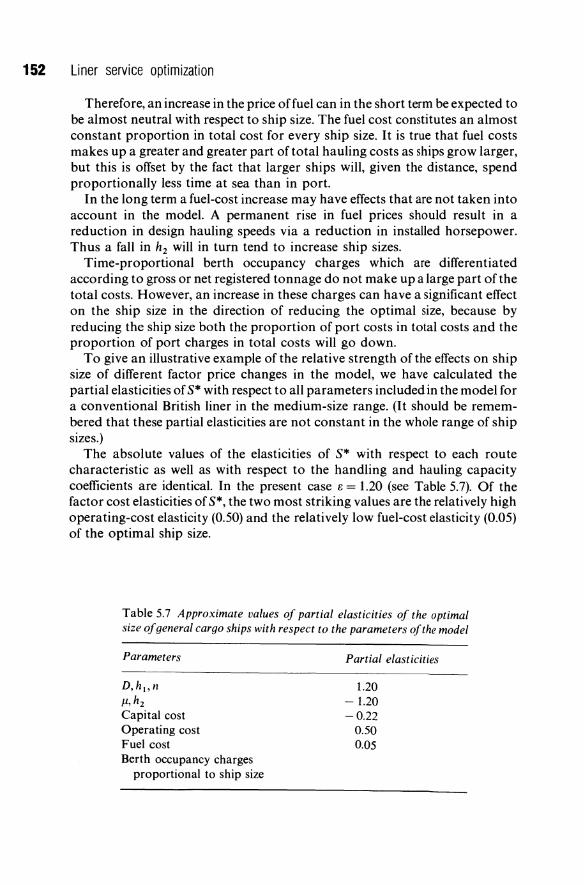
152 Liner service optimization
Therefore, an increase in the price of fuel can in the short term be expected to be almost neutral with respect to ship size. The fuel cost constitutes an almost constant proportion in total cost for every ship size. It is true that fuel costs makes up a greater and greater part of total hauling costs as ships grow larger, but this is offset by the fact that larger ships will, given the distance, spend proportionally less time at sea than in port.
In the long term a fuel-cost increase may have effects that are not taken into account in the model. A permanent rise in fuel prices should result in a reduction in design hauling speeds via a reduction in installed horsepower. Thus a fall in h2 will in turn tend to increase ship sizes.
Time-proportional berth occupancy charges which are differentiated according to gross or net registered tonnage do not make up a large part of the total costs. However, an increase in these charges can have a significant effect on the ship size in the direction of reducing the optimal size, because by reducing the ship size both the proportion of port costs in total costs and the proportion of port charges in total costs will go down.
To give an illustrative example of the relative strength of the effects on ship size of different factor price changes in the model, we have calculated the partial elasticities of S* with respect to all parameters included in the model for a conventional British liner in the medium-size range. (It should be remembered that these partial elasticities are not constant in the whole range of ship sizes.)
The absolute values of the elasticities of S* with respect to each route characteristic as well as with respect to the handling and hauling capacity coefficients are identical. In the present case e = 1.20 (see Table 5.7). Of the factor cost elasticities of S*, the two most striking values are the relatively high operating-cost elasticity (0.50) and the relatively low fuel-cost elasticity (0.05) of the optimal ship size.
Table 5.7 Approximate values of partial elasticities of the optimal size of general cargo ships with respect to the parameters of the model
Parameters
D,h 1 , /I
/1,h z Capital cost Operating cost Fuel cost Berth occupancy charges
proportional to ship size
Partial elasticities
1.20 -1.20 -0.22
0.50 0.05
Ship size and shipping costs 153
5.10.2 A ship size 'growth form' of the model
For predictive purposes it will rarely do to consider the influence of just one or a few ship-size determinants. All the partial elasticities have to be taken into account simultaneously when it comes to forecasting the future development of ship sizes.
It is convenient to give the model a standard 'growth form'. The dependent variable is the rate of growth. in ship size ('S*'), and independent variables are the rates of growth of all factor price and productivity parameters. The model can then be summarized:
where k represents hI' h2,Pi,Pj' qi and qj. Separate forecasts of the rate of growth of all the parameters, k, i.e. of the
development of factor prices and productivities have to be made. The combined effect on ship size growth is then obtained by summing up all the products of the partial elasticities and the forecast rates of growth of the independent variables.
5.10.3 Main factors behind the high rate of growth in ship size in recent times
It is beyond the scope of this study to test the ship-size growth form of the model on historical data of the ship size, factor price, and productivity developments. On the basis of the previous analysis it is, however, possible to pinpoint the likely main causes of some salient features of the development in ship size.
In the first half of this century it is believed that crew wage increases and crew productivity increases were by and large matching one another. Since the Second World War, however, at least so far as the traditional shipping nations - Britain, USA, Holland, and the Scandinavian countries - are concerned the development of seaman's wages has been inflationary, that is Pcrew
has grown at a higher rate than the rate of decline in qcrew. The fall in qcrew
which has occurred means that the manning requirement has gone down thanks to automation for each given ship size. On top of this the crew wage inflation has probably contributed quite considerably to the fall in the total demand for seamen by stimulating the growth in ship size, which has occurred since the war. Increasing the ship size is, as mentioned, one method of reducing the crew labour input per unit of output (ton of cargo).
The most important factor behind the high rate of growth in ship size since the war has, however, been capacity-increasing productivity improvement.
In recent times no very dramatic change in hz has occurred. This stands in vivid contrast to the development of hi. Since the war very significant
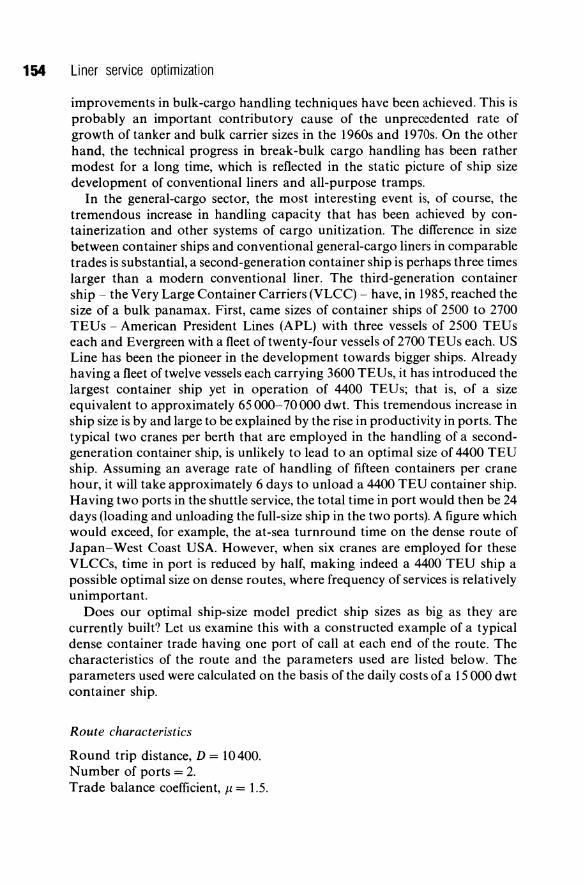
154 Liner service optimization
improvements in bulk-cargo handling techniques have been achieved. This is probably an important contributory cause of the unprecedented rate of growth of tanker and bulk carrier sizes in the 1960s and 1970s. On the other hand, the technical progress in break-bulk cargo handling has been rather modest for a long time, which is reflected in the static picture of ship size development of conventional liners and all-purpose tramps.
In the general-cargo sector, the most interesting event is, of course, the tremendous increase in handling capacity that has been achieved by containerization and other systems of cargo unitization. The difference in size between container ships and conventional general-cargo liners in comparable trades is substantial, a second-generation container ship is perhaps three times larger than a modern conventional liner. The third-generation container ship - the Very Large Container Carriers (VLCC) - have, in 1985, reached the size of a bulk panamax. First, came sizes of container ships of 2500 to 2700 TEUs - American President Lines (APL) with three vessels of 2500 TEUs each and Evergreen with a fleet of twenty-four vessels of 2700 TEU s each. US Line has been the pioneer in the development towards bigger ships. Already having a fleet of twelve vessels each carrying 3600 TEUs, it has introduced the largest container ship yet in operation of 4400 TEU s; that is, of a size equivalent to approximately 65000-70000 dwt. This tremendous increase in ship size is by and large to be explained by the rise in productivity in ports. The typical two cranes per berth that are employed in the handling of a secondgeneration container ship, is unlikely to lead to an optimal size of 4400 TEU ship. Assuming an average rate of handling of fifteen containers per crane hour, it will take approximately 6 days to unload a 4400 TEU container ship. Having two ports in the shuttle service, the total time in port would then be 24 days (loading and unloading the full-size ship in the two ports). A figure which would exceed, for example, the at-sea turnround time on the dense route of Japan-West Coast USA. However, when six cranes are employed for these VLCCs, time in port is reduced by half, making indeed a 4400 TEU ship a possible optimal size on dense routes, where frequency of services is relatively unimportant.
Does our optimal ship-size model predict ship sizes as big as they are currently built? Let us examine this with a constructed example of a typical dense container trade having one port of call at each end of the route. The characteristics of the route and the parameters used are listed below. The parameters used were calculated on the basis of the daily costs of a 15000 dwt container ship.
Route characteristics
Round trip distance, D = 10400. Number of ports = 2. Trade balance coefficient, J1. = 1.5.

Ship size and shipping costs 155
Output functions (daily)
Ton-miles, h2SE2 = 24 X 3.1251.17 where a 15000 dwt ship is assumed to travel at a speed of 16 miles per hour Tons loaded and unloaded, nh1SE1 = 24 x 19.55So. 3.
This assumes productivity of 350 tons per two crane-hour (thirty-five containers of 10 tons each) for a 15000 dwt vessel. Productivity is assumed to increase continuously with ship size by the one-third power of the ship size. This is mostly explained by using more cranes as ship size increases, which on average, for a large number of ships of each size, may lead to a continuous rise in handling productivity. Alternatively discrete number of cranes can be assumed to handle each range of ship sizes. For example, two cranes up to 15000 dwt, three for 15000-25000 dwt, etc.
Daily costs
Total capital costs, Plq1se 1 = 8.88So. 7 .
For a 15000 dwt this amounts to $7441 per day. This calculation is based on a price of $17 million for a newly built 15000 dwt container ship (quotation for
Table 5.8 The optimal ship size of a container ship on a dense route
Costs per ton Costs per ton Total costs in ports at sea per ton
Ship size ($) ($) ($)
3300 3.9066 45.1922 49.0988 3666 4.0564 43.2978 47.3542 4125 4.2335 41.3054 45.5389 4714 4.4462 39.2083 43.6545 5500 4.7098 36.9771 41.6869 6600 5.0489 34.5812 39.6301 8250 5.5096 31.9685 37.4781
11000 6.1910 29.0538 35.2448 16500 7.3604 25.6730 33.0334 25000 8.8948 22.9214 31.8162 30000 9.7070 21.9014 31.6085 31000 9.8637 21.7287 31.5924 32000 10.0187 21.5645 31.5832 33000* 10.1720* 21.4080* 31.5801 * 34000 10.3240 21.2587 31.5827 35000 10.4745 21.1160 31.5905 40000 11.2080 20.4880 31.6960 45000 11.9120 19.9710 31.8830
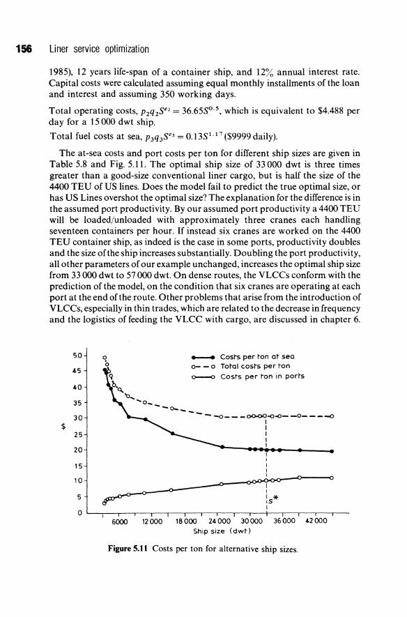
156 Liner service optimization
1985), 12 years life-span of a container ship, and 12% annual interest rate. Capital costs were calculated assuming equal monthly installments of the loan and interest and assuming 350 working days.
Total operating costs, P2Q2se2 = 36.65So. 5 , which is equivalent to $4.488 per day for a 15000 dwt ship.
Total fuel costs at sea, P3Q3se3 = 0.13S1.1 7 ($9999 daily).
The at-sea costs and port costs per ton for different ship sizes are given in Table 5.8 and Fig. 5.11. The optimal ship size of 33000 dwt is three times greater than a good-size conventional liner cargo, but is half the size of the 4400 TEU of US lines. Does the model fail to predict the true optimal size, or has US Lines overshot the optimal size? The explanation for the difference is in the assumed port productivity. By our assumed port productivity a 4400 TEU will be loaded/unloaded with approximately three cranes each handling seventeen containers per hour. If instead six cranes are worked on the 4400 TEU container ship, as indeed is the case in some ports, productivity doubles and the size ofthe ship increases substantially. Doubling the port productivity, all other parameters of our example unchanged, increases the optimal ship size from 33000 dwt to 57000 dwt. On dense routes, the VLCCs conform with the prediction of the model, on the condition that six cranes are operating at each port at the end ofthe route. Other problems that arise from the introduction of VLCCs, especially in thin trades, which are related to the decrease in frequency and the logistics of feeding the VLCC with cargo, are discussed in chapter 6.
$
50
45
40
35
30
25
20
15
10
5
o ;,
_ Cos~s per ton at sea
0- - 0 Total cos~s per ~on
0---0 Cos~s per ~on in ports
--- - -0- __ 00-00-0-0- -0_ ---0
s* I
6000 12000 18000 24000 30000 36000 42000 Ship size (dwt)
Figure 5.11 Costs per ton for alternative ship sizes.
6 Multi-port calling versus trans-shipment
6.1 THE GENERAL PROBLEM: FEEDER-TRANSPORT COST MINIMIZATION IN A GIVEN SERVICE RANGE
The cargo catchment area of a liner conference is best viewed as a stretch of coastline, because the depth of the catchment area is normally left undefined. We will call the cargo catchment area of a particular conference the 'service range' of the conference lines.
The service range (at each end ofthe trade route) is defined either simply as a naturally delimited seaboard of a country or continent like the Atlantic Coast of North America, or, when more exact borderlines in relation to service ranges of other conferences are required, as the seaboard between two given ports, e.g. the Hamburg-Dunkirk range. In either case all the ports to be included in the service (i.e. called at) are not given by the definition of the service range.
It is important to separate the problem of choice of service range from the problem of choice of ports-of-call, i.e. which ports are to be served. In this chapter we take the range for given, and consider only the second problem. In the last chapter of this part (chapter 9) the optimal extent of the service range is considered in a simultaneous minimization of shipping, port, and shippers' costs.
By introducing a somewhat wider definition offeeder transport than is usual the solution of the present problem can be regarded as a straightforward minimization of total feeder transport costs of the liner cargo generated in a given service range.
Each total door-to-door transport is a chain of a number of hauling and handling links. The hauling links can be divided into a trunk line link, and one or more feeder transport links. In the case of a liner-cargo shipment it may seem natural to define the start of the trunk line link where the shipment is loaded on to the liner, and to end where the discharge from the liner takes place. A more appropriate definition is, however, to regard only the sea crossing as the trunk line. Given the cargo catchment area of a liner service, the possible coast-wise cruising and multi-port calling by the liners are a substitute for inland-feeder transport or sea-feeder transport by separate ships.
6.2 THE SPECIFIC PROBLEM: THE POTENTIAL OF SEA-FEEDER TRANSPORT
In the thin-trade sector five to ten or even more calls per round voyage is common in break -bulk cargo shipping on longer routes. This practice has been
158 Liner service optimization
considered by many observers to be a rather costly way of collecting a full shipload together for the trunk haul.
If the cargo in question is easy to handle a shuttle service supported by seafeeder transport may be a viable solution to the thin-trade problem. Whilst trans-shipment has been a common practice in serving the more remote parts of the world (e.g. for shipping of oil), sea-feeder services have never been practised on a large scale in the liner shipping sector. However, already from the start of containerization it was commonly held that a shuttle-service pattern is inherently the least-cost solution of a container service (British Transport Docks Boards 1967). The required feeder transports could be performed by rail, road or sea, whichever turns out to be the cheapest mode in each particular case. Long-distance road transport of containers cannot compete with rail transport as soon as the annual volume of cargo is at all appreciable (Johnson and Garnett, 1971). Sea-feeder transport of unitized cargo is competitive to land-feeder transport, first, where a rail freightliner system does not exist for economic or geographical reasons, and, second, where a good deal of the cargo is generated in the proximity of seaports.
Lately sea-feeder transport of containers has been held up as an integral part of future optimal container transport systems in general (see chapter 8, section 8.2.3), and, more particularly, to be the solution to the old thin-trade problem aggravated by the increase in container ship size. The persistent continued practice of container shipping lines to call at an appreciable number of ports each round voyage may seem 'contrary to the basic idea of containerization', but is probably simply a sign that the point of balance between a trans-shipment solution and traditional multi-port calling is further to the advantage of the latter than has been expected on the basis of McKinney-style model results. Trans-shipping of cargo means that the direct handling costs per ton will be doubled. This is a severe disadvantage even for unitized cargo. Advocates of a shuttle-service/sea-feeder transport system seem to believe that this disadvantage will be offset by savings of the very expensive time of big trunk liners.
From the point of view of the conference lines operating in a particular trade the feeder transport problem can be summarized by the following three questions. Given the service range:
Which ports are to be included in the liner services, i.e. which ports are going to be 'conference ports'?
2 Of the included ports, which ports should be called at by the trunk liners? 3 How should the required feeder transport be organized for cargo generated
in the conference ports which are not called at by the trunk liners?
The solution to this three-phase problem can he either, (a) multi-port calling by the trunk liners at all ports declared to be conference ports, (b) a shuttle service between two 'base ports' at each end supported by sea-feeder transport

Multi-port calling versus trans-shipment 159
from the 'outports' on either side of the respective base ports, or (c) a 'mixed system' meaning that the liners call at more than one port at each end every round voyage, but not at all conference ports; feeder transports are arranged by the shipping lines for the cargo generated in the conference ports which are not called at by the trunk liners.
6.2.1 Comparative costs of the two extreme cases
By a schematic model we shall compare the costs of alternatives (a) and (b) above. In a following section alternative (c) will be discussed by a 'marginalis tic' approach; in that case the optimum solution is found by trying out different combinations starting from excluding the most unlikely 'marginal' port. Here we will consider the service range at one end of a containerized liner trade route, where a given number of ports are situated in the service range. In case a shuttle service is arranged, one port in the middle will be appointed the 'base port': this location ofthe base port is preferable from the point of view of feeder-transport distance minimization. The remaining ports on either side of the base port are called 'outports'. We will alllow for different proportions of the total cargo volume generated in the base port and in the outports, on one hand, and for differences in cargo volumes between different outports, on the other hand. In two respects, however, we will assume that all ports are similar, (a) the cargo handling performance is the same in all ports, and (b) the balance of import and export of liner cargo is the same in all ports, and consequently equal to the directional balance of the total trade flow on the route.
The consequences in terms of the trunk-liner's time requirements of making a diversion to call at a number of outports besides the base port can be divided into additional handling time, additional hauling time and additional transitory time, and be considered separately.
Additional time for actual cargo handling is insignificant. A given quantity of cargo is loaded and unloaded each round voyage no matter what the number of ports of call is. If a given number of cranes is used in each port -irrespective of whether a full shipload or a part load is handled - total effective handling time should be independent of the number of ports of call. In the RoRo case this holds true without reservation.
2 Considerable additional time at sea will be incurred by coastwise cruising in the service range.
3 Considerable additional transitory time will also be incurred by multi-port calling. The most reasonable assumption about this category of ships' time is that the transitory time per call at a particular port fluctuates widely in a random fashion but is, in principle, independent both of the ship size and the quantity of cargo loaded/unloaded in the port.
Against the costs of the additional time of multi-port calling diversions of the trunk liners, the costs ofthe total time of the feeder ships are to be put. We
160 Liner service optimization
assume that only one size - the optimal size for the total feeder transport task - is represented in the fleet of feeder ships.
(a) Simplifying assumptions regarding the size-elasticities of shipping costs and capacities
With the approach taken in the modelling of shipping costs in chapter 5, we need not specify the total time requirements either of the trunk liners, or of the feeder ships, but can express the comparative costs on a per ton basis directly. A strategic simplification of the model of chapter 5 is afforded by the following 'square-root approximation' of the ship-size elasticities of the handling and hauling costs per ton and ton-mile, respectively.
THE AVERAGE SIZE ELASTICITY OF THE HANDLING COSTS PER TON
(ei - Ed. It so happens that, provided that the berth occupancy charges are differentiated according to the size of the ships and that the value of the cargo is relatively high, the weighted average of the size-elasticities of the timeproportional costs incurred in port (see Table 5.5), just exceeds 0.7. We have previously concluded that the size-elasticities of the handling capacity is likely to range between 0.2 and 0.3 for general-cargo ships (see section 5.5.1). Assuming that a value close to the lower limit of his range applies to container ships, it follows that the size elasticity of the total indirect handling costs per ton is about 0.5.
THE AVERAGE SIZE ELASTICITY OF THE HAULING COSTS PER TON-MILE
(ej - E2)' The weighted average size elasticity of the main factor costs incurred per day at sea - the costs of capital, bunkers, crew etc. - is just above 0.6 (see Table 5.5). We have also concluded (see page 128) that the size elasticity of the hauling capacity is confined to the range of 1.00 to 1.17, and that the values applicable to liners are to be found in the upper-half range. Therefore, in view of the considerable facilitation of the calculations achieved, fixing the size elasticity ofthe total hauling costs per ton at the round figure of 0.5 seems well justified.
According to the 'square-root approximation' we thus have:
Indirect handling cost per ton = a 1 -j(S) ,
where S stands for ship size, and the proportionality constant a1 incorporates the level of port productivity;
I· '1 1 Hau mg cost per ton-ml e = a 2 -j(S) .
To get the hauling cost per ton the hauling cost per ton-mile is to be multiplied by the round-voyage distance, and divided by the directional cargo balance factor, J1.. As before the coast-to-coast route distance is denoted by D.

Multi-port calling versus trans-shipment 161
We will now make explicit use of the concept of the 'gross round-voyage distance' which was developed in chapter 5 in the discussion of transitory time. By converting the total expected transitory time per round voyage to voyage miles, and adding these 'miles' to the actual (net) nautical miles of the round voyage, the gross distance, G, is obtained. The round-voyage G of a shuttle service is consequently equal to 2D plus the transitory time in port at both ends converted to miles.
In the comparison of the multi-port calling costs per ton with the costs per ton ofa shuttle-service/sea-feeder transport system, we will only go into details of one service range. The organization of the operations in the other service range is held constant throughout the comparison. It is therefore inappropriate to include the transitory time suffered at the other end in the round voyage distance 2D; to get the gross distance G only the transitory time suffered in the service range at one end has to be added.
(b) The comparative costs excluding the direct handling costs
The ports of call in the service range under study are numbered from one end to the other 1 ... k . .. n, where the kth port is the base port, which will be used in case a shuttle service supported by sea-feeder transports is organized. Any port in the sequence of ports including the base port is called the ith port, and any port in the sequence of port excluding the base port is called the jth port. The distance from each port to the base port is denoted d~. The distance of feeder transport of export and import between an outport and the base port is consequently equal to 2d~.
The distance between successive pairs of ports included in the service is denoted d: + l' In the multi-port calling case the coastwise cruising distance is assumed to be equal to the sum of all these distances.
The expected transitory time per call converted to miles at sea is denoted t; or tj depending on the context.
We can then define the following gross distances.
GROSS DIST ANCES
Shuttle service round-voyage gross distance,
Multi-port calling diversion gross distance,
Round-voyage gross distance of feeder transports to serve the jth port,
A verage round-voyage gross distance of feeder transports,
G1 =2D + t k • n n
ci1 = I d:+ 1 + I t j . i=l Uk
n
I QPd~+tj+tk) G f = ,,--U~k ---:-n----
I Qj Uk
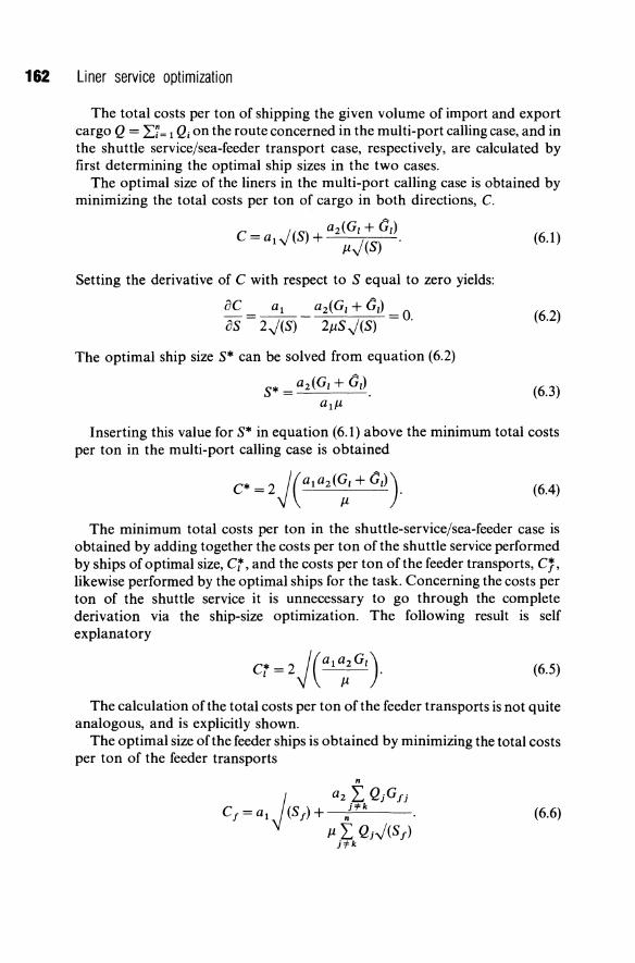
162 Liner service optimization
The total costs per ton of shipping the given volume of import and export cargo Q = Li = 1 Qi on the route concerned in the multi-port calling case, and in the shuttle service/sea-feeder transport case, respectively, are calculated by first determining the optimal ship sizes in the two cases.
The optimal size of the liners in the multi-port calling case is obtained by minimizing the total costs per ton of cargo in both directions, C.
C = I(S) a2(GI + Gl )
a1v + JlJ(S)
Setting the derivative of C with respect to S equal to zero yields:
ac =~_ a2(GI + Gl) =0 as 2.,)(S) 211.8 J(S) .
The optimal ship size S* can be solved from equation (6.2)
S* = a2 (GI + Gl ).
a1Jl
(6.1)
(6.2)
(6.3)
Inserting this value for S* in equation (6.1) above the minimum total costs per ton in the multi-port calling case is obtained
(6.4)
The minimum total costs per ton in the shuttle-service/sea-feeder case is obtained by adding together the costs per ton of the shuttle service performed by ships of optimal size, ct, and the costs per ton of the feeder transports, Cj, likewise performed by the optimal ships for the task. Concerning the costs per ton of the shuttle service it is unnecessary to go through the complete derivation via the ship-size optimization. The following result is self explanatory
(6.5)
The calculation of the total costs per ton of the feeder transports is not quite analogous, and is explicitly shown.
The optimal size of the feeder ships is obtained by minimizing the total costs per ton of the feeder transports
(6.6)
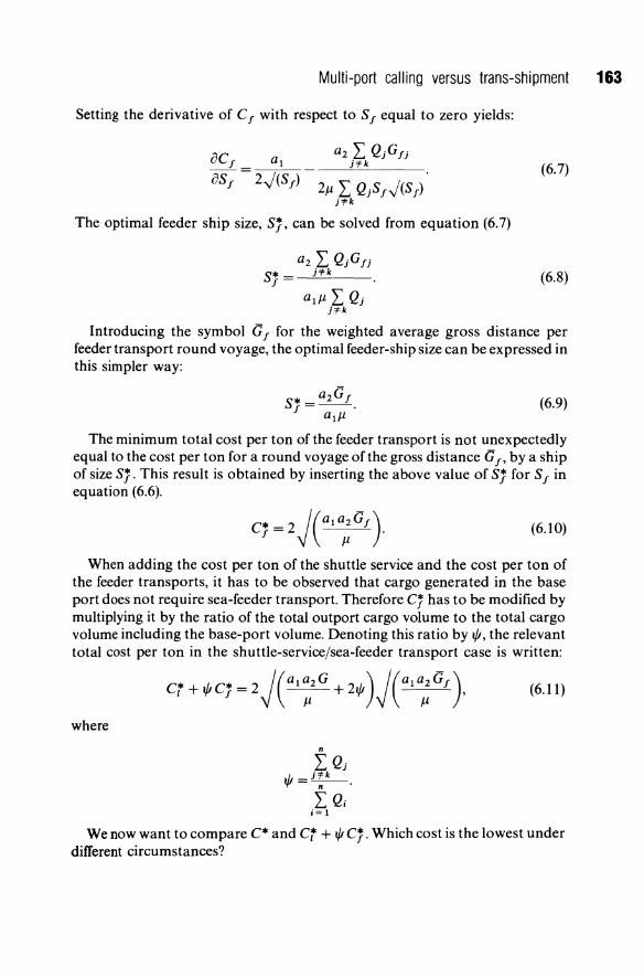
Multi-port calling versus trans-shipment 163
Setting the derivative of C f with respect to Sf equal to zero yields:
2/1 L QjS f.j(S f) Hk
The optimal feeder ship size, Sj, can be solved from equation (6.7)
a 1 /1 L Qj Hk
(6.7)
(6.8)
Introducing the symbol Gf for the weighted average gross distance per feeder transport round voyage, the optimal feeder-ship size can be expressed in this simpler way:
S* _ a2 Gf f - a1 /1
(6.9)
The minimum total cost per ton of the feeder transport is not unexpectedly equal to the cost per ton for a round voyage of the gross distance G f' by a ship of size Sj. This result is obtained by inserting the above value of Sj for Sf in equation (6.6).
(6.10)
When adding the cost per ton of the shuttle service and the cost per ton of the feeder transports, it has to be observed that cargo generated in the base port does not require sea-feeder transport. Therefore Cj has to be modified by multiplying it by the ratio of the total outport cargo volume to the total cargo volume including the base-port volume. Denoting this ratio by tjJ, the relevant total cost per ton in the shuttle-servicejsea-feeder transport case is written:
ct + tjJCj = 2 J (a 1 : 2 G + 2tjJ )J (a 1 a~ Gf ). (6.11)
where
We now want to compare C* and ct + tjJ Cj. Which cost is the lowest under different circumstances?
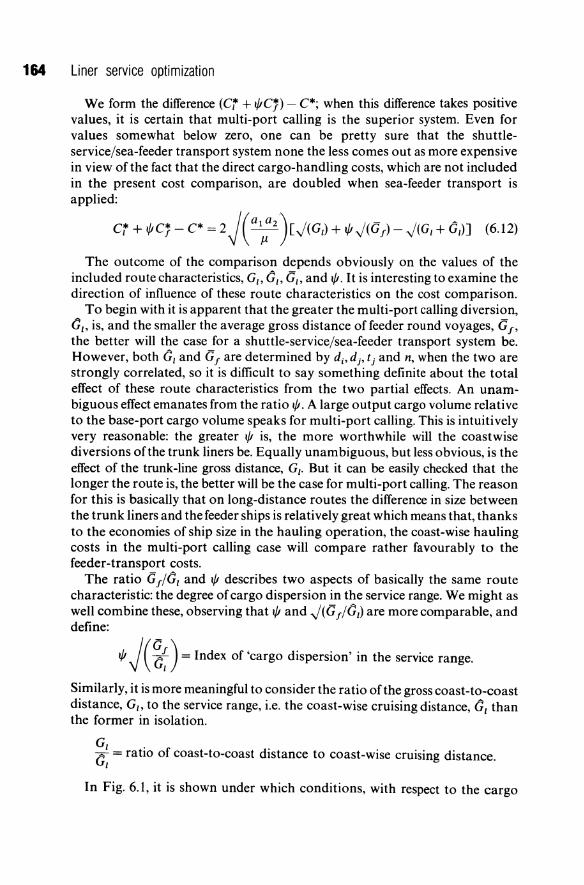
164 Liner service optimization
We form the difference (Cr + I/ICj) - C*; when this difference takes positive values, it is certain that multi-port calling is the superior system. Even for values somewhat below zero, one can be pretty sure that the shuttleservice/sea-feeder transport system none the less comes out as more expensive in view of the fact that the direct cargo-handling costs, which are not included in the present cost comparison, are doubled when sea-feeder transport is applied:
Cr + I/ICj - C* = 2 J (a1;2) [J(GI) + I/IJ(af ) - J(GI + GI)] (6.12)
The outcome of the comparison depends obviously on the values of the included route characteristics, GI , GI , ai' and 1/1. It is interesting to examine the direction of influence of these route characteristics on the cost comparison.
To begin with it is apparent that the greater the multi-port calling diversion, GI , is, and the smaller the average gross distance of feeder round voyages, a f' the better will the case for a shuttle-service/sea-feeder transport system be. However, both GI and af are determined by di,d j , tj and n, when the two are strongly correlated, so it is difficult to say something definite about the total effect of these route characteristics from the two partial effects. An unambiguous effect emanates from the ratio 1/1. A large output cargo volume relative to the base-port cargo volume speaks for multi-port calling. This is intuitively very reasonable: the greater 1/1 is, the more worthwhile will the coastwise diversions ofthe trunk liners be. Equally unambiguous, but less obvious, is the effect of the trunk-line gross distance, GI . But it can be easily checked that the longer the route is, the better will be the case for multi-port calling. The reason for this is basically that on long-distance routes the difference in size between the trunk liners and the feeder ships is relatively great which means that, thanks to the economies of ship size in the hauling operation, the coast-wise hauling costs in the multi-port calling case will compare rather favourably to the feeder-transport costs.
The ratio a f/GI and 1/1 describes two aspects of basically the same route characteristic: the degree of cargo dispersion in the service range. We might as well combine these, observing that 1/1 and J(a f/GI) are more comparable, and define:
1/1 J ( ~ ) = Index of 'cargo dispersion' in the service range.
Similarly, it is more meaningful to consider the ratio of the gross coast-to-coast distance, GI , to the service range, i.e. the coast-wise cruising distance, GI than the former in isolation.
G . G: = ratIo of coast-to-coast distance to coast-wise cruising distance.
In Fig. 6.1, it is shown under which conditions, with respect to the cargo
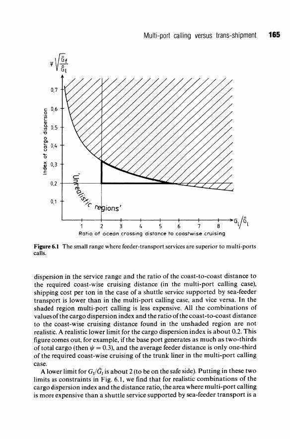
0,7
5 0,6
~ QJ
~ D,S "ii o 0> o 0,4 u
'0 ~ 0,3 "C c:
0,1
Multi-port calling versus trans-shipment 165
2 3 4 5 6 7 8 Raho of ocean crossing distance to coastwise cruising
Figure 6.1 The small range where feeder-transport services are superior to multi-ports calls.
dispersion in the service range and the ratio of the coast-to-coast distance to the required coast-wise cruising distance (in the multi-port calling case), shipping cost per ton in the case of a shuttle service supported by sea-feeder transport is lower than in the multi-port calling case, and vice versa. In the shaded region multi-port calling is less expensive. All the combinations of values of the cargo dispersion index and the ratio of the coast-to-coast distance to the coast-wise cruising distance found in the unshaded region are not realistic. A realistic lower limit for the cargo dispersion index is about 0.2. This figure comes out, for example, if the base port generates as much as two-thirds of total cargo (then t/J = 0.3), and the average feeder distance is only one-third of the required coast-wise cruising of the trunk liner in the multi-port calling case.
A lower limit for Gt/(J/ is about 2 (to be on the safe side). Putting in these two limits as constraints in Fig. 6.1, we find that for realistic combinations of the cargo dispersion index and the distance ratio, the area where multi-port calling is more expensive than a shuttle service supported by sea-feeder transport is a
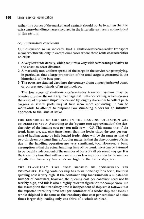
166 Liner service optimization
rather tiny corner of the market. And again, it should not be forgotten that the extra cargo-handling charges incurred in the latter alternative are not included in this picture.
( c) Intermediate conclusions
Our discussion so far indicates that a shuttle-service/sea-feeder transport seems worthwhile only in exceptional cases where these route characteristics co-exist:
1 A very low trade density, which requires a very wide service range relative to the coast-to-coast distance.
2 A markedly non-uniform spread of the cargo in the service range implying, in particular, that a large proportion of the total cargo is generated in the hinterland of the base port.
3 The ports are situated deep into the country along a much-indented coast, or on scattered islands of an archipelago.
The low score of shuttle-service/sea-feeder transport systems may be counter intuitive; the main argument against multi-port calling, which stresses the waste of expensive ships' time caused by lengthy diversions to collect partcargoes in several ports may at first seem more convincing. It can be worthwhile to attempt to pinpoint two stumbling blocks for an intuitive approach to the issue at stake.
THE ECONOMIES OF SHIP SIZE IN THE HAULING OPERATION ARE
UNDERESTIMATED. According to the 'square-root approximation' the sizeelasticity of the hauling cost per ton-mile is = - 0.5. This means that if the trunk liners are, say, nine times larger than the feeder ships, the cost per tonmile of hauling cargo by fully loaded feeder ships will be the same as that of two-thirds-empty trunk liners. Another matter is that the diseconomies of ship size in the handling operation are very significant, too. However, a basic assumption is that the actual handling time of the trunk liners can be assumed to be roughly independent of the number of ports of call per round voyage. It is the transitory time that will increase more or less in proportion to the number of calls. But transitory time costs are high for the feeder ships, too.
THE TRANSITORY TIME COST SHOULD BE CONSIDERED PER
CONT AINER. If a big container ship has to wait one day for a berth, the total queuing cost is very high. If the container ship loads/unloads a substantial number of containers, however, the queuing cost per container need not be terribly high, and this is also a highly relevant figure for the comparison. On the assumption that transitory time is independent of ship size it follows that the expected transitory time cost per container of a feeder ship that loads a whole shipload is the same as the transitory time cost per container of a nine times larger ship loading only one-third of a whole shipload.

Multi-port calling versus trans-shipment 167
6.2.2 A marginalistic approach
The problem of multi-port calling versus a shuttle-service/sea-feeder transport system has so far been discussed in 'either/or' terms. This must not obscure the fact that a mixed system is an interesting alternative in many trades, where the cargo base is markedly unevenly distributed between the ports of a service range. An extreme output in a deep-sea trade may well be best served by trans-shipment if only a modest volume of cargo is generated in the port, without all the other ports having to be served in the same way.
The previous model for calculation of the comparative shipping costs of pure multi-port calling and a shuttle-service/sea-feeder transport system is useful also when a marginalistic approach is taken. When we want to examine whether a 'marginal port' should be dropped from the itinerary of the trunk liners, and instead be served by sea-feeder transport to the nearest trunk-liner port of call, the gross diversion distances Gl is replaced by the diversion required solely on account of a call at the jth port, Glj , and the average gross feeder-transport distance, Gf , is replaced by the gross feeder-transport distance from thejth port to the nearest port of call, G fj' The trunk-liner gross distance, G l , should not be interpreted as the shuttle-service distance now, but as the gross round-voyage distance of the liners including calls at outports except for the jth port.
The value oft/! now represents the ratio of the cargo volume generated at the jth port to the total cargo volume of the trade. This ratio can now be much lower than assumed in Fig. 6.1. The horizontal boundary line can be moved downwards considerably, and the area where sea-feeder transport is a feasible alternative will increase downwards in the diagram. On the other hand, the relevant ratio of the gross distance to the diversion required to call at the marginal port on the horizontal axis, is in most realistic cases much greater than 2, so the previous lower limit is now moved forward to the right in Fig. 6.1. The meaning of all this is simple enough: the likelihood that a marginal port should be skipped by the trunk liners (and served by feeder transport) increases with, (a) decreases in the proportion of the total cargo generated in the marginal port, and (b) increases in the relative (to the total round voyage) diversion necessary to call at the marginal port. To give some examples, the model predicts that when the cargo generated in the marginal port is no more than 5, 10, 15, or 20% of the total cargo, the required diversion must not be more than approximately 1 %, respectively, of the gross distance of the round voyage to make it worthwhile.
( a) Variability in demand - some further considerations regarding 'marginal ports'
One interesting aspect of this problem is the importance of variations over time in the cargo volume generated in a marginal port. The best can be made of the fact that such variations occur by exercising a certain amount of flexibility in the itinerary from one round voyage to another.

168 Liner service optimization
The core of the idea is to regard a particular marginal port as a 'groupage depot', and hold it open to the last possible day each round, whether or not a call will actually be made at the marginal port. If very little cargo has arrived at the marginal port one particular round, it is cheaper to haul this quantity of cargo by another means of transport - road, rail, or sea-feeder transportto a nearby port, which normally generates a sufficient quantity of cargo to warrant a call, than to make a separate call at the marginai port. Figure 6.2 depicts the essentials of the matter.
A basic premise of the situation at hand is that the jth port has just passed the test for inclusion in the liner services. In other words, it has been established that the sum of the additional inland-feeder-transport costs, which the shippers would incur ifthejth port were excluded, exceeds the incremental cost of the diversion (in the form of cruising time and/or transitory time) required for calling at thejth port. The horizontal line of Fig. 6.2 gives the level of the incremental cost per call at the jth port. This cost is independent of the quantity of cargo loaded/unloaded, Qj' since it is assumed that this quantity will be handled anyway but not necessarily in the jth port. The upper digressively increasing curve represents the cost of the cheapest feeder (land or sea) transport alternative of Qj to and from a nearby port of call.
It is assumed that the quantity of cargo generated in the jth port fluctuates such that it sometimes is less than Qj (see Fig. 6.2), and sometimespresumably more often otherwise the port should not have been included in the first place - is greater than Qj" Ifless cargo than Qj is expected (the quantity
$
I'" IQ· I )
I Qj
(2) Total cost of feeder transport between the j th port and a nearby port of call
(1) Incremental cost of a call at t"he j th port"
Figure 6.2 Costs per round voyage, (1) calling at the jth port, and (2) hauling the cargo generated in the jth port to/from a nearby port of call.
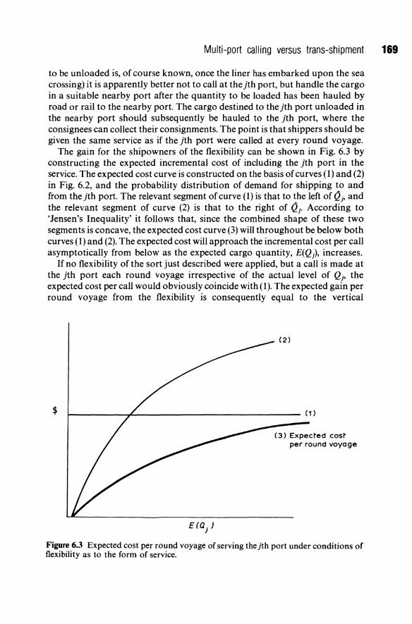
Multi-port calling versus trans-shipment 169
to be unloaded is, of course known, once the liner has embarked upon the sea crossing) it is apparently better not to call at the jth port, but handle the cargo in a suitable nearby port after the quantity to be loaded has been hauled by road or rail to the nearby port. The cargo destined to the jth port unloaded in the nearby port should subsequently be hauled to the jth port, where the consignees can collect their consignments. The point is that shippers should be given the same service as if the jth port were called at every round voyage.
The gain for the shipowners of the flexibility can be shown in Fig. 6.3 by constructing the expected incremental cost of including the jth port in the service. The expected cost curve is constructed on the basis of curves (1) and (2) in Fig. 6.2, and the probability distribution of demand for shipping to and from the jth port. The relevant segment of curve (1) is that to the left of (L, and the relevant segment of curve (2) is that to the right of Qj. According to 'Jensen's Inequality' it follows that, since the combined shape of these two segments is concave, the expected cost curve (3) will throughout be below both curves (1) and (2). The expected cost will approach the incremental cost per call asymptotically from below as the expected cargo quantity, E(Q), increases.
If no flexibility of the sort just described were applied, but a call is made at the jth port each round voyage irrespective of the actual level of Qj' the expected cost per call would obviously coincide with (1). The expected gain per round voyage from the flexibility is consequently equal to the vertical
$
(2)
r---------~---------------------------- (1)
(3) Expec~ed cos~ per round voyage
Figure 6.3 Expected cost per round voyage of serving the jth port under conditions of flexibility as to the form of service.
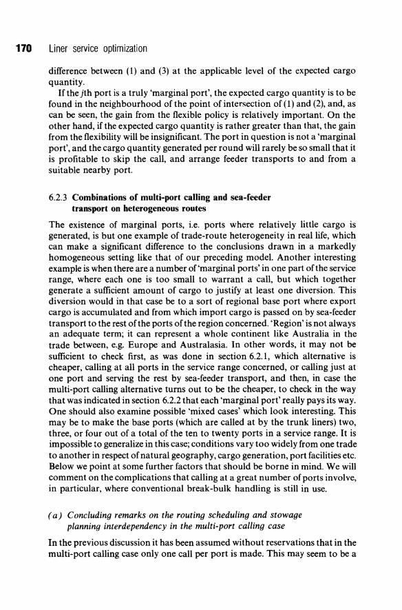
170 Liner service optimization
difference between (1) and (3) at the applicable level of the expected cargo quantity.
Uthejth port is a truly 'marginal port', the expected cargo quantity is to be found in the neighbourhood of the point of intersection of (1) and (2), and, as can be seen, the gain from the flexible policy is relatively important. On the other hand, if the expected cargo quantity is rather greater than that, the gain from the flexibility will be insignificant. The port in question is not a 'marginal port', and the cargo quantity generated per round will rarely be so small that it is profitable to skip the call, and arrange feeder transports to and from a suitable nearby port.
6.2.3 Combinations of multi-port calling and sea-feeder transport on heterogeneous routes
The existence of marginal ports, i.e. ports where relatively little cargo is generated, is but one example of trade-route heterogeneity in real life, which can make a significant difference to the conclusions drawn in a markedly homogeneous setting like that of our preceding model. Another interesting example is when there are a number of 'marginal ports' in one part ofthe service range, where each one is too small to warrant a call, but which together generate a sufficient amount of cargo to justify at least one diversion. This diversion would in that case be to a sort of regional base port where export cargo is accumulated and from which import cargo is passed on by sea-feeder transport to the rest of the ports of the region concerned. 'Region' is not always an adequate term; it can represent a whole continent like Australia in the trade between, e.g. Europe and Australasia. In other words, it may not be sufficient to check first, as was done in section 6.2.1, which alternative is cheaper, calling at all ports in the service range concerned, or calling just at one port and serving the rest by sea-feeder transport, and then, in case the multi-port calling alternative turns out to be the cheaper, to check in the way that was indicated in section 6.2.2 that each 'marginal port' really pays its way. One should also examine possible 'mixed cases' which look interesting. This may be to make the base ports (which are called at by the trunk liners) two, three, or four out of a total of the ten to twenty ports in a service range. It is impossible to generalize in this case; conditions vary too widely from one trade to another in respect of natural geography, cargo generation, port facilities etc. Below we point at some further factors that should be borne in mind. We will comment on the complications that calling at a great number of ports involve, in particular, where conventional break-bulk handling is still in use.
( a) Concluding remarks on the routing scheduling and stowage planning interdependency in the multi-port calling case
In the previous discussion it has been assumed without reservations that in the multi-port calling case only one call per port is made. This may seem to be a
Multi-port calling versus trans-shipment 171
rather strong assumption at closer scrutiny at least in cases where the number of ports of call is relatively great. Some final comments on certain relevant problems which so far have been left out of consideration can be appropriate.
In particular so far as a break-bulk cargo shipping is concerned, the choice of ports of call for a particular service can be rather difficult owing to the complicated interrelationships between routing, scheduling and stowage planning. With containerization the skill of stowage planning has to some extent become redundant, due to the possibility of container 'shifting'.
To give flavour of the intricacy of a meticulous optimization of a break-bulk liner service a few comments on the interdependency of routing, scheduling and stowage planning will be made. In deep-sea trades it is usual that liners call at some eight to ten ports per round voyage. This causes very tricky problems of operations analysis. In which order are the ports to be called at? How is the cargo to be stowed in order to minimize the sum of handling time and hauling time? Moreover, these questions have to be given answers which are consistent with a viable schedule, i.e. the time span between ships (given the ship size) has to be such that the demand for hold space is adequately matched. Consider a ship steaming fully loaded towards the first port of call, port 1, in a range of ports, where the cargo is to be discharged, but also where cargo for the backhaul is to be loaded. It is obviously a great advantage for the shipowner to avoid calling twice at port 1, i.e. once for unloading, and once for loading on the return. This is easily accomplished if one hold is reserved for cargo destined to and originating from port 1; if the cargo to be discharged in port 1 is concentrated in one hold, the total handling speed will be lower compared to a situation where a number of holds are being worked simultaneously. Spreading out cargo destined to port 1 over several holds, on the other hand, may require a second call at port 1 for the loading of cargo, unless this cargo is quantitatively insignificant.
It should also be mentioned that the stowage planning has to take stability aspects into account. For instance, it may seem pertinent to stow cargo destined to a particular port vertically and along the whole ship-side with a view to working every hold simultaneously, and avoid calling twice at the same port. However, such 'lop-sided' emptying of the ship is not possible for stability reasons.
6.3 THE VERY LARGE CONTAINER CARRIERS (VLCC) AND FEEDER SERVICES
The introduction of the VLCCs has forced shipping lines to call at fewer base ports, and rely to a greater extent on feeder services. Several lines have introduced around the world service combined with their VLCCs. Evergreen operates twenty-four ships in their round-the-world service (R WS) - twelve in the eastbound and twelve in the westbound leg. US Line operates twelve ships in the R WS, and there are others which, on a smaller scale, provide R WS - the Danish Barbar Blue Line, the Belgium ABC line, the Singaporian Neptune

172 Liner service optimization
Orient Line (NOL), and the Hong Kong based Orient Oversea Container Line (OOCL). When VLCC ships are used in these services (or indeed elsewhere) such as the US Line's 4400 TEUs and Evergreen's 2700 TEUs, the pattern that is envisaged is of the big vessels calling at few ports (San FranciscoYokohama, for example) and feeder services - by land or sea - transporting the cargo to the base port. Producers' economies of ship size, it is hoped, will be made possible by the smooth efficient feeder services that would fill the VLCC.
Against this, our feeder-services model delivers the following message: do not overrate the savings in costs by substituting sea-feeder transport for multiport calling by ocean liners, and do not underrate the extra costs of double handling. Technically, the system of a shuttle service provided by VLCC, supported by feeder services, look quite appealing, but cost comparisons speak a different language.
The only conceivable way by which these VLCC can survive, is by increasing their own share at the expense of others. Their time-proportional share of cargo will probably have to be tripled, to fill the ship. This may well be possible to achieve on dense routes. Approximately four ships depart daily from Yokohama to the US West coast. Replacing these by one or two VLCC may be obtained without imposing extra costs to shippers due to lower frequency.
On other thin-trade routes, the VLCC would mean either too high feeder costs or else too low frequency service - both undermining the chances of success of the VLCC.
7 Shippers' costs of sailings infrequency and transit time
The greatest problems in the optimization of the liner shipping serving a particular trade are associated with the quantification of shippers' costs. In chapter 5 we have already dealt with the interest costs of cargo in transit. In this chapter we move ashore and examine some other items of shippers' costs which will rise by a lowering of the sailings frequency and/or increase in transit time.
The fact that there is a shorter or longer interval between the placing of an order overseas and the date of delivery gives rise to costs to shippers of, in principle, three different kinds, depending on the type of goods.
A lengthening of delivery times takes the form of an increase in the storage costs.
2 A lengthening of delivery times takes the form of disruption costs for the importers/users of goods which are not stored by them.
3 A lengthening of delivery times takes the form of a decrease in value of the traded goods.
The first-mentioned type of cost is the only one really susceptible to monetary quantification. Therefore, the following discussion is largely about storage costs. At the end of the chapter some further comments are made on the nature of the other two types of cost.
7.1 STORAGE COSTS
Generally speaking, the storage of goods is often necessary because the rate of production and the rate of consumption of the goods are more or less illmatched. Two extreme examples are storage of agricultural products, which are forthcoming in a short harvest period, and storage of seasonal sport equipment like skis, which may be produced at a fairly constant rate throughout the year, but used only during a relatively short period. Over the business cycle large stocks are built up and run down in all industry with the purpose of maintaining capacity utilization and employment at a reasonably constant level.
This main type of stockholding is not relevant in the present connection. Here we shall focus on the storage costs which are dependent on transportservice characteristics. Then we shall go into more specialized storage functions.
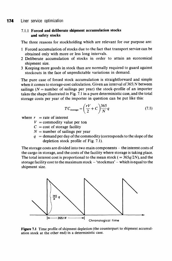
174 Liner service optimization
7.1.1 Forced and deliberate shipment accumulation stocks and safety stocks
The three reasons for stockholding which are relevant for our purpose are:
Forced accumulation of stocks due to the fact that transport service can be obtained only with more or less long intervals.
2 Deliberate accumulation of stocks in order to attain an economical shipment size.
3 Keeping more goods in stock than are normally required to guard against stockouts in the face of unpredictable variations in demand.
The pure case of forced stock accumulation is straightforward and simple when it comes to storage-cost calculation. Given an interval of 365/ N between sailings (N = number of sailings per year) the stock-profile of an importer takes the shape illustrated in Fig. 7.1 in a pure deterministic case, and the total storage costs per year of the importer in question can be put like this:
( rv )365 TCstorage = 2 + C N q
where r = rate of interest V = commodity value per ton C = cost of storage facility N = number of sailings per year
(7.1)
q = demand per day of the commodity (corresponds to the slope of the depletion stock profile of Fig. 7.1).
The storage costs are divided into two main components - the interest costs of the cargo in storage, and the costs of the facility where storage is taking place. The total interest cost is proportional to the mean stock ( = 365q/2N), and the storage facility cost to the maximum stock - 'stockmax' - which is equal to the shipment size.
·1 Chronological ~ime
Figure 7.1 Time profile of shipment depletion (the counterpart to shipment accumulation stock at the other end) in a deterministic case.
Shippers' costs 175
7.1.2 Trade-offs for different categories of shippers
The pure-and-simple case above is seldom wholly relevant, because few shippers would choose to send or receive shipments continuously. The transport costs per ton of small shipments is normally higher than of larger shipments mainly for two reasons: there are certain costs which are by and large fixed per shipment, and so far as full-shipload shipments are concerned, the freight rate per ton is decreasing with shipment size because of economies of ship size.
In the inventory management literature costs which will increase almost commensurately with the number of deliveries per year are commonly referred to as 'billing cost', although the cost for general documentation is not the only cost which is basically fixed per shipment. The cost of the inland transport from the port to the importer's warehouse is also a cost which is almost fixed per shipment as long as the shipment size does not exceed a full truckload, or a full container when applicable. For convenience we use the name 'billing cost', B, for the costs which can be assumed to be fixed per shipment.
The optimal pattern of deliveries is that which minimizes the total storage, billing and freight costs, given the annual volume of import, Q ( = 365q). The main control variable is the number of shipments per year received by the importer in question, n, and a main constraint on the optimization problem is supposedly the sailings frequency, N, so far as shippers of general cargo are concerned. We can write total shipper's cost in the two cases of general cargo and bulk cargo in this way:
( rv )Q TCgeneral cargo = 2 + C -;;- + nB + QF (7.2)
where n < N
TCbu1k = (r; + C )~+ nB+ QF(~} (7.3)
The two differences between general cargo and bulk shippers are, (a) that the latter can choose without constraints when shipments are to be dispatched, and (b) the freight rate per ton (F) is a decreasing function of bulk cargo shipment ( = shipload) size.
For bulk-cargo shippers the tapering off offreight costs with respect to ship size is such an important effect that the trade-off often results in quite large voluntary 'shipment accumulation' stocks. When it comes to general-cargo shippers, the control variable n does not appear in the freight-cost term, but only in the storage-cost and billing-cost terms. It is obvious that the trade-off of part-load shippers, i.e. users of liner shipping services, results in far less stockholding than in the case of bulk cargo. This does not mean that storage costs are unimportant in liner shipping service optimization. The cargo is
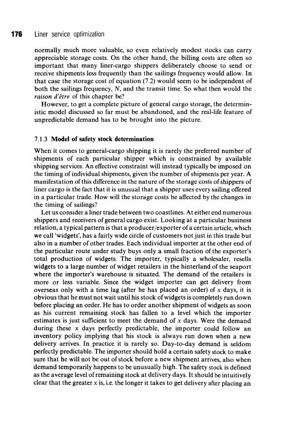
176 Liner service optimization
normally much more valuable, so even relatively modest stocks can carry appreciable storage costs. On the other hand, the billing costs are often so important that many liner-cargo shippers deliberately choose to send or receive shipments less frequently than the sailings frequency would allow. In that case the storage cost of equation (7.2) would seem to be independent of both the sailings frequency, N, and the transit time. So what then would the raison d'etre of this chapter be?
However, to get a complete picture of general cargo storage, the deterministic model discussed so far must be abandoned, and the real-life feature of unpredictable demand has to be brought into the picture.
7.1.3 Model of safety stock determination
When it comes to general-cargo shipping it is rarely the preferred number of shipments of each particular shipper which is constrained by available shipping services. An effective constraint will instead typically be imposed on the timing of individual shipments, given the number of shipments per year. A manifestation of this difference in the nature of the storage costs of shippers of liner cargo is the fact that it is unusual that a shipper uses every sailing offered in a particular trade. How will the storage costs be affected by the changes in the timing of sailings?
Let us consider a liner trade between two coastlines. At either end numerous shippers and receivers of general cargo exist. Looking at a particular business relation, a typical pattern is that a producer/exporter of a certain article, which we call 'widgets', has a fairly wide circle of customers not just in this trade but also in a number of other trades. Each individual importer at the other end of the particular route under study buys only a small fraction of the exporter's total production of widgets. The importer, typically a wholesaler, resells widgets to a large number of widget retailers in the hinterland of the seaport where the importer's warehouse is situated. The demand of the retailers is more or less variable. Since the widget importer can get delivery from overseas only with a time lag (after he has placed an order) of x days, it is obvious that he must not wait until his stock of widgets is completely run down before placing an order. He has to order another shipment of widgets as soon as his current remaining stock has fallen to a level which the importer estimates is just sufficient to meet the demand of x days. Were the demand during these x days perfectly predictable, the importer could follow an inventory policy implying that his stock is always run down when a new delivery arrives. In practice it is rarely so. Day-to-day demand is seldom perfectly predictable. The importer should hold a certain safety stock to make sure that he will not be out of stock before a new shipment arrives, also when demand temporarily happens to be unusually high. The safety stock is defined as the average level of remaining stock at delivery days. It should be intuitively clear that the greater x is, i.e. the longer it takes to get delivery after placing an
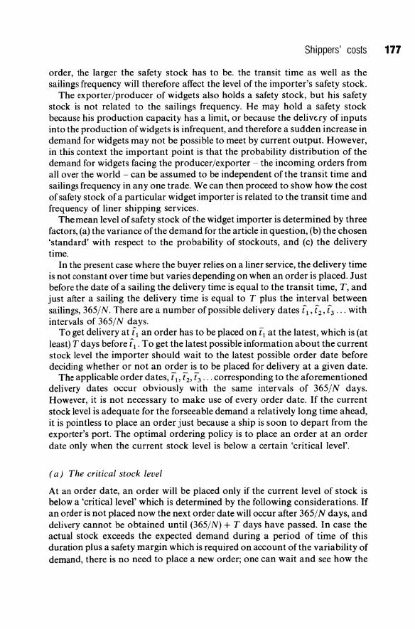
Shippers' costs 177
order, the larger the safety stock has to be. the transit time as well as the sailings frequency will therefore affect the level of the importer's safety stock.
The exporter/producer of widgets also holds a safety stock, but his safety stock is not related to the sailings frequency. He may hold a safety stock because his production capacity has a limit, or because the delivf..fy of inputs into the production of widgets is infrequent, and therefore a sudden increase in demand for widgets may not be possible to meet by current output. However, in this context the important point is that the probability distribution of the demand for widgets facing the producer/exporter - the incoming orders from all over the world - can be assumed to be independent of the transit time and sailings frequency in anyone trade. We can then proceed to show how the cost of safety stock of a particular widget importer is related to the transit time and frequency of liner shipping services.
The mean level of safety stock of the widget importer is determined by three factors, (a) the variance of the demand for the article in question, (b) the chosen 'standard' with respect to the probability of stock outs, and (c) the delivery time.
In the present case where the buyer relies on a liner service, the delivery time is not constant over time but varies depending on when an order is placed. Just before the date of a sailing the delivery time is equal to the transit time, T, and just after a sailing the delivery time is equal to T plus the interval between sailings, 365/ N. There are a number of possible delivery dates t1 , t2 , G ... with intervals of 365/ N days.
To get delivery at tl an order has to be placed on f1 at the latest, which is (at least) T days before t1 • To get the latest possible information about the current stock level the importer should wait to the latest possible order date before deciding whether or not an order is to be placed for delivery at a given date.
The applicable order dates, fl' f2' t3'" corresponding to the aforementioned delivery dates occur obviously with the same intervals of 365/N days. However, it is not necessary to make use of every order date. If the current stock level is adequate for the forseeable demand a relatively long time ahead, it is pointless to place an order just because a ship is soon to depart from the exporter's port. The optimal ordering policy is to place an order at an order date only when the current stock level is below a certain 'critical level'.
(a) The critical stock level
At an order date, an order will be placed only if the current level of stock is below a 'critical level' which is determined by the following considerations. If an order is not placed now the next order date will occur after 365/ N days, and delivery cannot be obtained until (365/N) + T days have passed. In case the actual stock exceeds the expected demand during a period of time of this duration plus a safety margin which is required on account of the variability of demand, there is no need to place a new order; one can wait and see how the

178 Liner service optimization
situation is at the following order date. The safety margin should be determined according to a chosen standard with respect to the probability of stock outs.
The safety margin can be calculated by using Chebyshev's Inequality, which states that the probability of a random variable, X, taking a value which differs from the expected value, E(X), by more than K standard deviations, is less than 1/K2. If a standard is set implying that the probability of stockouts must not exceed P, and assuming a symmetrically distributed demand, it follows that the safety margin has to be 1/.J(2P) standard deviations of the expected demand. Denoting the variance Var(X), the safety margin is thus equal to .J [Var( X)/2P].
The safety margin does not constitute the whole safety stock as previously defined. To derive a useful expression for the safety stock, let us assume that the daily rate of demand is a random variable, q, which is independent of the previous actual development of demand. The variance of the daily demand is written S2. On these assumptions the expected demand during a period of time of (365/N) + T days (e.g. from tl to (2 in Fig. 7.2 and the corresponding variance are q(365/N + T), and s2(365/N + T), respectively.
The critical stock level can then be specified thus:
Critical stock level = (3!5 + T)q + sJ[(365/~ + TJ. (7.4)
(b) Safety stock as afunction of transit time and sailings frequency
At the date of delivery, (2 in Fig. 7.2, the expected level of stock (just before replenishment) is equal to the expected level of stock at the date when the order was placed, t2 in Fig. 7.2, minus the expected demand during the delivery time,
An order is placed
'\1 I
t2 t, Calendar ~ime
Figure 7.2 A segment of the stock time profile during which an order is placed and delivery occurs.

Shippers' costs 179
which is equal to qT. The fact that an order was placed at t;. indicates that the level of stock was below the critical level at this particular order date. The critical level can have been hit at any date between tl and t2. On average the level of stock should have fallen to the critical level at a date just between two consecutive order dates. This means that on delivery day just before replenishment the stock is expected to equal the critical level minus (365/2N + T)q. We have defined the safety stock as the expected stock just before replenishment. We thus have:
365 J[(365/N) + T] Safety stock = q 2N + s 2P . (7.5)
As is seen, the safety stock is greater than the 'safety margin' included in the critical stock level. The reason for the addition of the product of half the interval between sailings and q is that the delivery dates occur with a certain interval. If delivery could be obtained at any day only provided that the order is placed T days before, the critical stock level would be equal to the safety margin.
Using this expression for the safety stock to make expression (7.2) above for the total costs of general-cargo shippers more complete, we can write:
TC = c: + C )~ + (rV + C){2~ + s J[(365~~ + T]} + nB + QF.
(7.6)
The sailings frequency, N, is a determinant of the safety stock, but not ofthe shipment accumulation stock unless the choice ofthe number of shipments, n, is constrained by N. It is also noteworthy that the safety stock is independent of n. The number of shipments is determined by a trade-off of billing costs against the costs of shipment accumulation stock without regard to the safety stock.
In the main case of liner-cargo shipping the effect on storage costs of a change in the sailings frequency is revealed as a change in the costs of safety stocks only. Further insight into this relationship will be gained by making certain specifications by which a numerical example can be considered.
( c) Numerical example
Suppose first that the probability distribution of demand adheres to the Poisson distribution. Then the standard deviation is equal to the square root of the mean: s = J(q), and the safety stock amounts to:
Safety stock in Poisson case = JL + J[(Q/N) + (TQ/365)]. (7.7) 2N 2P
Next we will fix certain values of T and P. On a deep-sea route the transit time (including loading and unloading time in port) is several weeks. Let us
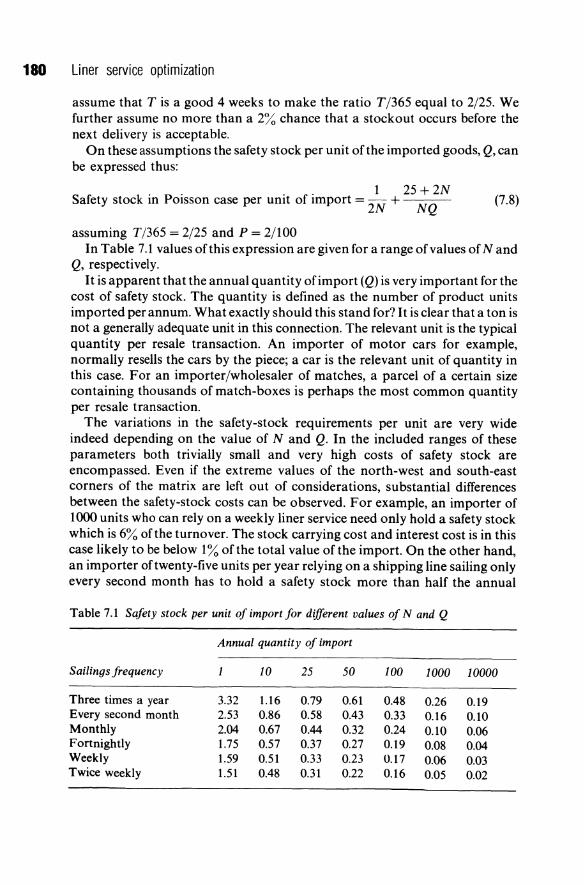
180 Liner service optimization
assume that T is a good 4 weeks to make the ratio T/365 equal to 2/25. We further assume no more than a 2% chance that a stockout occurs before the next delivery is acceptable.
On these assumptions the safety stock per unit of the imported goods, Q, can be expressed thus:
. 1 25 + 2N Safety stock in Poisson case per unit of Import = 2N + NQ (7.8)
assuming T/365 = 2/25 and P = 2/100 In Table 7.1 values of this expression are given for a range of values of Nand
Q, respectively. It is apparent that the annual quantity of import (Q) is very important for the
cost of safety stock. The quantity is defined as the number of product units imported per annum. What exactly should this stand for? It is clear that a ton is not a generally adequate unit in this connection. The relevant unit is the typical quantity per resale transaction. An importer of motor cars for example, normally resells the cars by the piece; a car is the relevant unit of quantity in this case. For an importer/wholesaler of matches, a parcel of a certain size containing thousands of match-boxes is perhaps the most common quantity per resale transaction.
The variations in the safety-stock requirements per unit are very wide indeed depending on the value of Nand Q. In the included ranges of these parameters both trivially small and very high costs of safety stock are encompassed. Even if the extreme values of the north-west and south-east corners of the matrix are left out of considerations, substantial differences between the safety-stock costs can be observed. For example, an importer of 1000 units who can rely on a weekly liner service need only hold a safety stock which is 6% of the turnover. The stock carrying cost and interest cost is in this case likely to be below 1 % of the total value of the import. On the other hand, an importer oftwenty-five units per year relying on a shipping line sailing only every second month has to hold a safety stock more than half the annual
Table 7.1 Safety stock per unit of import for different values of Nand Q
Annual quantity of import
Sailings frequency 1 10 25 50 100 1000 10000
Three times a year 3.32 1.16 0.79 0.61 0.48 0.26 0.19 Every second month 2.53 0.86 0.58 0.43 0.33 0.16 0.10 Monthly 2.04 0.67 0.44 0.32 0.24 0.10 0.06 Fortnightly 1.75 0.57 0.37 0.27 0.19 0.08 0.04 Weekly 1.59 0.51 0.33 0.23 0.17 0.06 0.03 Twice weekly 1.51 0.48 0.31 0.22 0.16 0.05 0.02

Shippers' costs 181
turnover, which will cost him nearly 10% of the total value. As regards highvalue goods this cost is well above the normal freight rate. A number of interesting features of the pattern of safety-stock requirements is revealed by the matrix.
Successive halvings of the sailings frequency have an accelerated effect on the safety-stock requirements. For all except the very big importer the safety-stock requirements will increase by less than 20% as a result of reducing the frequency from twice a week to a fortnightly service, while a further four-fold reduction to sailings every second month will increase the safety-stock requirements by 60-70%. This supports the general view of many liner-service operators that a lower frequency than fortnightly sailings is unacceptable, while it is almost inconsequential for shippers if more than one sailing per week is offered - at least in a deep-sea trade.
2 The safety stock requirement of very small importers would be almost prohibitive if the assumed standard with respect to the probability of stockouts is maintained. This standard is likely to be lowered considerably when the import quantity is only a couple of units per year, and in the extreme case no stock is held at all, but the article in question is not ordered until the need for it has actually arisen. The latter category of import will apparently not fall under the present main heading: 'Cargo for which costs of a low-sailings frequency are revealed as storage costs', and is consequently taken up in the next section.
3 The safety-stock requirements of a very big shipper is almost trivial unless the sailings frequency is extremely low. The very big importer is likely to want to receive many shipments per year. According to a well-known formula the optimal number of shipments is proportional to the square root of the annual turnover. In case Q is very large it thus can happen that the sailings frequency becomes an effective constraint on the choice of N. Under such circumstances the cost of safety stock is not the only item of the total storage cost which depends on N. To this case we now turn.
7.1.4 Additional costs of shipment accumulation stock when the sailings frequency imposes a constraint on the number of shipments
A shipper who uses the liner services on the route practically every sailing, can be assumed to dispatch a smaller number of shipments per year than he would like. For such a shipper N will affect both the shipment accumulation stock and the safety stock. The relationship between costs of accumulation stock and N can be expressed as the costs of deviating from the optimal stock in an unconstrained situation.
In a case where the sailings frequency is not an effective constraint the optimal number of shipments, n *, is found by taking the first derivative of total shipper's costs, TC, as written in equation (7.6), with respect to n, setting the
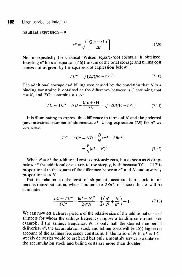
182 Liner service optimization
resultant expression = 0
* = J[Q(C + rv)] n 2B'
(7.9)
Not unexpectedly the classical 'Wilson square-root formula' is obtained. Inserting n* for n in equation (7.6) the sum ofthe total storage and billing cost comes out as given by the square-root expression below:
TC* = J[2BQ(c + rV)]. (7.10)
The additional storage and billing cost caused by the condition that N is a binding constraint is obtained as the difference between TC assuming that n = N, and TC* assuming n < N:
TC - TC* = NB + Q(c2:rV) - J[2BQ(c + rV)]. (7.11)
It is illuminating to express this difference in terms of N and the preferred (unconstrained) number of shipments, n*. Using expression (7.9) for n* we can write:
TC - TC* = NB + B n*2 - 2Bn* N
B =~n*-N)2.
N (7.12)
When N = n* the additional cost is obviously zero, but as soon as N drops below n* the additional cost starts to rise steeply, both because TC - TC* is proportional to the square of the difference between n* and N, and inversely proportional to N.
Put in relation to the cost of shipment, accumulation stock in an unconstrained situation, which amounts to 2Bn*, it is seen that B will be eliminated:
TC - TC* _ (n* - N)2 _ ~(n* N) _ TC* - 2n*N -2 N+n* 1. (7.13)
We can now get a clearer picture of the relative size of the additional costs of shippers for whom the sailings frequency impose a binding constraint. For example, if the sailings frequency, N, is only half the desired number of deliveries, n*, the accumulation stock and billing costs will be 25% higher on account of the sailings frequency constraint. If the ratio of N to n* is 1:4-weekly deliveries would be preferred but only a monthly service is available -the accumulation stock and billing costs are more than doubled.
Shippers' costs 183
7.2 COSTS OF SAILINGS INFREQUENCY AND TRANSIT TIME FOR GOODS WHICH ARE NOT STORED BY IMPORTERS
Some liner cargo is not likely to be stored at all in the importing country. In this case the relationship between shippers' costs and the delivery time cannot be easily estimated. The typical importer of this type of cargo is a producer of goods or services. Traders, wholesalers/importers are normally not interested to deal in goods which are demanded so infrequently and irregularly that the storage costs per unit are bound to be rather high.
If a certain input article used in the production process by a firm is expected to be badly needed at frequently occurring occasions, the firm is likely to hold a safety stock. A goods manufacturing enterprise holds, aside from the stocks of input material, stocks of tools and equipment which are quantitatively important in the production process. It is, however, uneconomic to have spare items of everything. The smaller the required number of items of a particular tool or equipment is from experience, and the more irregularly the need arises, the less likely it is that items are held in store.
When an accident happens and some special equipment breaks down beyond repair the cost caused by the interruption can be very substantial indeed. This is an inevitable fact oflife of goods production; one cannot afford a complete plant in reserve, standing idle most of the time. Therefore, there exist articles in liner cargo which are not stored by the importers, and are not ordered until the need for the articles actually occurs.
An attempt to quantify the expected costs of delivery time of such articles will obviously encounter serious difficulties. By the nature of the type of articles concerned each case is a 'special case'.
Two approaches to at least a partial quantification of these costs should, however, be mentioned. First, an upper limit to the delivery time costs can perhaps be assumed to be constituted by the hypothetical costs of safety stocks. The person who knows the costs of delivery time best in each particular case is the importer himself. The fact that he does not store a particular article should imply that he expects the costs of a safety stock to be greater than the costs of the risk of occasionally being short of the article in question.
Secondly, it may be possible to get an idea of how importers would evaluate a change in delivery time for goods which are not stored by them from the observed propensity, under different circumstances, of these importers to resort to the many times more expensive alternative of air transport.
7.3 LOSS OF VALUE OF PERISHABLE GOODS
We can define perishable goods as goods the quality of which deteriorates with the passage of time. The shorter the time lag between production and consumption is, the higher will be the value of such goods in the hands of the consumers. One time lag is constituted by the transit time, and another by the
184 Liner service optimization
storage time. All efforts should be aimed at minimizing the storage time. Exporters of perishable goods should send as many shipments per unit of time as the sailing frequency allows. Shipment accumulation on account of billing costs is normally not contemplated.
The transit time is one inevitable component of the total time lag between production and consumption. On the assumption that both the rate of production and the rate of consumption are roughly constant over time, the other time lag will on average be equal to the interval between sailings. (Half the time lag occurs in the exporting country and half the time lag occurs in the importing country.)
The introduction of refrigerated holds of ships as well as storage facilities, and the advances in refrigeration techniques have mitigated quite radically the loss of value in transit or storage of certain foodstuffs like meat. The capacity costs of ships and storage facilities have, on the other hand, gone up.
The natural and best approach to a quantification of the delivery-time costs of perishable foodstuff is simply to read off the market evaluation of different qualities with respect to freshness of a certain kind of goods. Other types of 'perishable' goods are mail, newspapers, magazines and the like. Mention can, finally, be made of goods which fall in value because a general slump occurs in the market concerned during the time in transit. In the days when trans-ocean transport took several months a very important cost of time for delivery used to be the risk for a price fall on commodity exchanges in the importing country. To guard against this risk futures markets have arisen. Nowadays this is a less important aspect so far as liner shipping is concerned. Transit times are much shorter and the proportion in liner cargo of primary products which can suddenly rise or fall in price has decreased.
7.4 HOW IMPORT ANT ARE SHIPPERS' COSTS?
How important are shippers' costs? Will their inclusion in the total costs per ton affect significantly the optimal size of the ship? To answer these questions we will construct an example of container services in a thin trade. We take our example at the end of chapter 5 as a starting point. The round trip distance is 10400 miles and the trade is served by two ports - one at each end of the route. This is a simplification since there will be more than two ports of call in a thin trade, but which would not significantly alter the results. All other parameters are as described in pages 154-156. We take the low port-productivity figure of 350 tons per hour (two cranes handling together thirty-five containers of 10 tons each per hour), which yielded an optimal ship size of 33000 dwt. The trade volume on the dense leg is equal to the size of the optimal ship (33000 dwt) times the annual frequency of sailings (ten), which gives a total of 330 000 tons annually. Trade is not balanced. Trade on the thin leg is half in volume, i.e. 165000 tons. To measure the effect of users' costs we consider alternative frequencies (or what are implied ship sizes), holding the total volume of trade
Shippers' costs 185
unchanged. Thus, we will compare the costs of one ship of 33000 dwt, two ships of 16 500 dwt, three ships of 11 000 dwt etc. For each alternative we will calculate the shipping-company costs per ton (producers' costs), and the shippers' costs per ton (users' costs), which include the interest costs of cargo in transit and the costs of safety stock. The optimal ship size is the one that brings the sum of the shipping company's costs per ton and the shippers' costs per ton to a minimum. The calculation of the shipping company's costs was discussed in chapter 5 and will not be repeated here. The calculation of the users' costs per ton needs more explanation.
The interest costs on cargo in transit varies with the size ofthe ship. Similar to the costs of capital and crew, they are incurred all the time - at sea and in ports - and can be treated in a similar way. Let us denote: r = the interest rate per ton per day; v = the average value of ton of cargo per day. The interest costs per ton of cargo in transit, Cr , is equal to:
[ rvS DrvS ] Cr = n(h 1SE') + j.lh 2SE2 (7.14)
where all other notations are as explained in chapter 5. Total interest costs (the numerator) increase in proportion to the size of the ship, S. This is so for both ports and at sea. It equals the interest costs, r, times the average value per ton, v, times the number of tons carried, S. The interest costs per ton in ports (the first term) rise with the ship size because E1 (which we assumed in the example to take a value of 0.3) is less than the interest cost ship-size elasticity (which equals unity). Interest costs per ton at sea decline with ship size, since E2 equals 1.1 7.
In the calculation of the costs of safety stock, we assume that demand facing each importer follows the Poisson distribution, and we can write the safety stock in the Poisson case as:
S ~ k (Q) J[(Q/N) + (TQ/365)] a ety stoc = 2N + 2P (7.15)
(see equation (7.7». The costs of safety stock per ton for alternative frequencies (and ship sizes)
was calculated using equation (7.15), making the following assumptions:
The costs of safety stock is incurred by each importer, and should be calculated separately for each one. The aggregate costs of safety stock is then arrived at by adding up the costs of safety stock of all importers. This calculation should be carried out separately for importers at each end of the route.
2 The price per ton of the safety stock includes the interest costs on goods in storage plus the charges for the actual storage.
The values of the parameters needed for the calculation are listed below. We have tested the sensitivity of the results to alternative values of two

186 Liner service optimization
parameters - the average value of cargo per ton, and the interest rate. We therefore conducted nine-ship optimization for each combination of interest rate and value of cargo.
Values of parameters required to calculate shippers' costs:
{Rl = 10%
Annual interest rate, R R2 = 12% R3 = 14%
which assuming 350 operating days of the ship gives:
{rl = 0.00029
Interest rate per day, r r 2 = 0.00034. r3 = 0.0004
Alternative values per ton of cargo were considered for the following range:
Raw materials: value per container, $10000 value per container, $20000 value per container, $30000.
Leather and cloths: TVs:
Assuming the same utilization for all three, of 12 tons per container,
{
Vl = $833.333 The value per ton of cargo, v V 2 = $1666.666.
V3 = $2500.000
The daily interest costs per ton, rv, for these alternative combinations, are summarized in Table 7.2.
The round-trip time is 36 days, and the frequency of service, N, is 10. Delivery time, T, is half the round-trip time, and equals 18 days. Although
Table 7.2 Interest costs per ton per day, rv,for alternative values of interest rates and values of cargo
v($)
833.333 1666.666 2500.000
r
0.1
0.2381 0.4762 0.7143
0.12
0.2857 0.5714 0.8571
0.14
0.3333 0.6666 1.00
Storage charges per ton were calclated on the basis of $5 per day per container and a utilization of 12 tons per container.
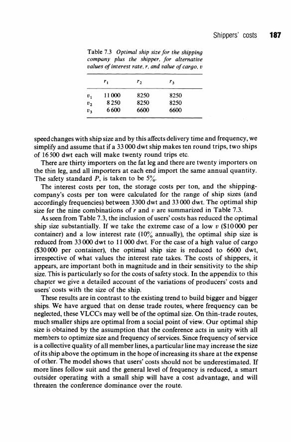
Table 7.3 Optimal ship size for the shipping company plus the shipper, for alternative values of interest rate, r, and value of cargo, v
11000 8250 6600
8250 8250 6600
8250 8250 6600
Shippers' costs 187
speed changes with ship size and by this affects delivery time and frequency, we simplify and assume that if a 33000 dwt ship makes ten round trips, two ships of 16500 dwt each will make twenty round trips etc,
There are thirty importers on the fat leg and there are twenty importers on the thin leg, and all importers at each end import the same annual quantity, The safety standard P, is taken to be 5%,
The interest costs per ton, the storage costs per ton, and the shippingcompany's costs per ton were calculated for the range of ship sizes (and accordingly frequencies) between 3300 dwt and 33000 dwt. The optimal ship size for the nine combinations of r and v are summarized in Table 7,3.
As seen from Table 7.3, the inclusion of users' costs has reduced the optimal ship size substantially. If we take the extreme case of a low v ($10000 per container) and a low interest rate (10% annually), the optimal ship size is reduced from 33000 dwt to 11000 dwt. For the case of a high value of cargo ($30000 per container), the optimal ship size is reduced to 6600 dwt, irrespective of what values the interest rate takes. The costs of shippers, it appears, are important both in magnitude and in their sensitivity to the ship size. This is particularly so for the costs of safety stock. In the appendix to this chapter we give a detailed account of the variations of producers' costs and users' costs with the size of the ship.
These results are in contrast to the existing trend to build bigger and bigger ships. We have argued that on dense trade routes, where frequency can be neglected, these VLCCs may well be of the optimal size. On thin-trade routes, much smaller ships are optimal from a social point of view. Our optimal ship size is obtained by the assumption that the conference acts in unity with all members to optimize size and frequency of services. Since frequency of service is a collective quality of all member lines, a particular line may increase the size of its ship above the optimum in the hope of increasing its share at the expense of other. The model shows that users' costs should not be underestimated. If more lines follow suit and the general level of frequency is reduced, a smart outsider operating with a small ship will have a cost advantage, and will threaten the conference dominance over the route.
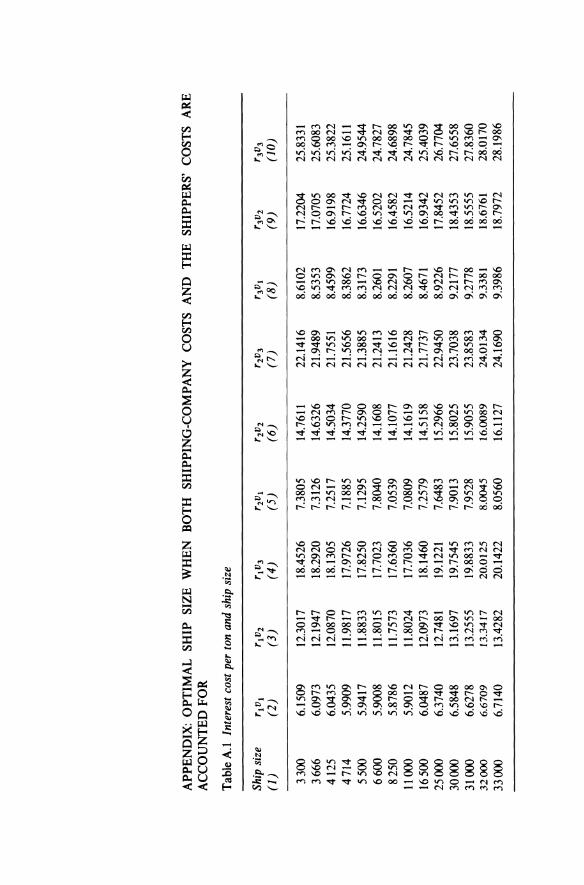
APP
EN
DIX
: O
PT
IMA
L
SH
IP
SIZ
E
WH
EN
B
OT
H
SH
IPP
ING
-CO
MP
AN
Y
CO
STS
AN
D
TH
E
SH
IPP
ER
S'
CO
STS
AR
E
AC
CO
UN
TE
D F
OR
Tab
le A
.l In
tere
st c
ost
per
ton
and
ship
siz
e
Ship
siz
e r 1
v 1
r 1v 2
r 1
v 3
r 2v 1
r 2
v 2
r2v 3
r 3
v l
r 3v 2
r3
v 3
(1)
(2)
(3)
(4)
(5)
(6)
(7)
(8)
(9)
(10
)
3300
6.
1509
12
.301
7 18
.452
6 7.
3805
14
.761
1 22
.141
6 8.
6102
17
.220
4 25
.833
1 36
66
6.09
73
12.1
947
18.2
920
7.31
26
14.6
326
21.9
489
8.53
53
17.0
705
25.6
083
4125
6.
0435
12
.087
0 18
.130
5 7.
2517
14
.503
4 21
.755
1 8.
4599
16
.919
8 25
.382
2 47
14
5.99
09
11.9
817
17.9
726
7.18
85
14.3
770
21.5
656
8.38
62
16.7
724
25.1
611
5500
5.
9417
11
.883
3 17
.825
0 7.
1295
14
.259
0 21
.388
5 8.
3173
16
.634
6 24
.954
4 66
00
5.90
08
11.8
015
17.7
023
7.80
40
14.1
608
21.2
413
8.26
01
16.5
202
24.7
827
8250
5.
8786
11
.757
3 17
.636
0 7.
0539
14
.107
7 21
.161
6 8.
2291
16
.458
2 24
.689
8 11
000
5.90
12
11.8
024
17.7
036
7.08
09
14.1
619
21.2
428
8.26
07
16.5
214
24.7
845
1650
0 6.
0487
12
.097
3 18
.146
0 7.
2579
14
.515
8 21
.773
7 8.
4671
16
.934
2 25
.403
9 25
000
6.37
40
12.7
481
19.1
221
7.64
83
15.2
966
22.9
450
8.92
26
17.8
452
26.7
704
3000
0 6.
5848
13
.169
7 19
.754
5 7.
9013
15
.802
5 23
.703
8 9.
2177
18
.435
3 27
.655
8 31
000
6.62
78
13.2
555
19.8
833
7.95
28
15.9
055
23.8
583
9.27
78
18.5
555
27.8
360
32
00
0
6.67
09
13.3
417
20.0
125
8.00
45
16.0
089
24.0
134
9.33
81
18.6
761
28.0
170
3300
0 6.
7140
13
.428
2 20
.142
2 8.
0560
16
.112
7 24
.169
0 9.
3986
18
.797
2 28
.198
6

Tab
le A
.2
Cos
ts o
f sti
fety
sto
ck a
nd s
hip
size
Safe
ty s
tock
per
im
port
er
Cos
ts o
f saf
ety
stoc
k pe
r to
n (t
on
s)
($)
Ship
siz
e T
hin
leg
Den
se l
eg
WI V
I W
IV2
WIV
3 W
2VI
W2V
2 W
2V3
W3
VI
W3V
2 W
3V
3
3300
0 67
9.06
3 52
4.27
1 28
.711
9 39
.152
2 49
.592
5 30
.799
1 43
.326
6 55
.854
1 32
.886
3 47
.501
0 62
.120
0 16
500
380.
627
297.
726
16.2
008
22.0
919
27.9
827
17.3
786
24.4
473
31.5
160
18.5
563
26.8
027
35.0
516
1100
0 27
9.89
3 22
1.12
3 11
.974
1 16
.328
2 20
.682
3 12
.844
6 18
.069
1 23
.293
6 13
.715
0 19
.810
0 25
.906
8 82
50
229.
190
182.
531
9.84
57
13.4
256
17.0
057
10.5
613
14.8
571
19.1
529
11.2
770
16.2
885
21.3
015
6600
19
8.64
0 15
9.26
5 8.
5629
11
.676
5 14
.790
1 9.
1853
12
.921
4 16
.657
5 9.
8078
14
.166
3 18
.526
2 55
00
178.
214
143.
702
7.70
50
10.5
067
13.3
084
8.26
51
11.6
269
14.9
887
8.82
52
12.7
471
16.6
702
4714
16
3.59
2 13
2.55
9 7.
0908
9.
6691
12
.247
5 7.
6062
10
.700
0 13
.793
9 8.
1217
11
.730
9 15
.341
3 41
25
152.
608
124.
186
6.62
93
9.03
99
11.4
505
7.11
12
10.0
037
12.8
962
7.59
32
10.9
675
14.3
430
3666
14
4.05
3 11
7.66
3 6.
2699
8.
5498
10
.829
7 6.
7257
9.
4614
12
.l970
7.
1815
10
.372
9 13
.565
3 33
00
137.
202
112.
439
5.98
20
8.15
73
10.3
325
6.41
69
9.02
70
11.6
371
6.85
18
9.89
67
12.9
425
Col
umn
2 is
cal
cula
ted
by u
sing
equ
atio
n (1
6).
Col
umn
3 is
cal
cula
ted
by m
ulti
plyi
ng th
e pr
ice
per
ton
per d
ay o
f the
hol
ding
sto
ck, w
, by
the
annu
al q
uant
ity
times
the
num
ber
of im
port
ers
times
350
day
s di
vide
d by
the
ann
ual
quan
tity
of
all
impo
rter
s.
w, is
the
sum
of
the
inte
rest
rat
e pe
r to
n pe
r da
y, r
, pl
us t
he r
enta
l st
orag
e co
sts
per
ton
per
day.
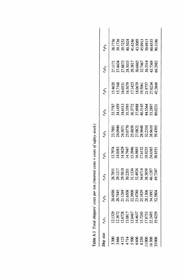
Tab
le A
.3
Tot
al s
hipp
ers'
cost
s pe
r to
n (i
nter
est
cost
s +
cost
s o
f saf
ety
stoc
k)
Ship
siz
e rt
vt
rtvz
r t
v 3
rZv t
rz
vz
r Zv 3
r 3
V t
r3v Z
r3
v 3
3300
12
.132
9 20
.459
0 28
.785
1 13
.797
4 23
.788
1 33
.778
7 15
.462
0 27
.117
1 38
.775
6 36
66
12.3
672
20.7
445
29.1
217
14.0
383
24.0
940
34.1
459
15.7
168
27.4
434
39.1
736
4125
12
.672
8 21
.126
9 29
.581
0 14
.362
9 24
.507
1 34
.651
3 16
.053
1 27
.887
3 39
.725
2 47
14
13.0
817
21.6
508
30.2
201
14.7
947
25.0
770
35.3
595
16.5
079
28.5
033
40.5
024
5500
13
.646
7 22
.390
0 31
.133
4 15
.394
6 25
.885
9 36
.377
2 17
.142
5 29
.381
7 41
.624
6 66
00
14.4
637
23.4
780
32.4
924
16.9
893
27.0
822
37.8
988
18.0
679
30.6
865
43.3
089
8250
15
.724
3 25
.182
9 34
.671
4 17
.615
2 28
.964
8 40
.314
5 19
.506
1 32
.746
7 45
.991
3 llO
OO
17.8
753
28.1
306
38.3
859
19.9
255
32.2
310
44.5
364
21.9
757
36.3
314
50.6
913
1650
0 22
.249
5 34
.189
2 46
.128
7 24
.636
5 38
.961
0 53
.289
7 27
.023
4 43
.736
9 60
.455
5 33
000
35.4
259
52.5
804
69.7
347
38.8
551
59.4
393
80.0
231
42.2
849
66.2
982
90.3
186
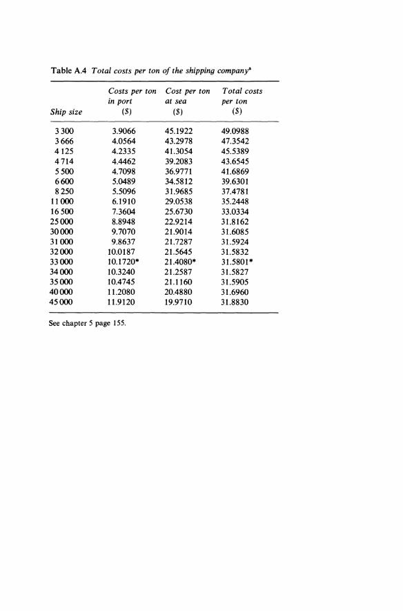
Table A.4 Total costs per ton of the shipping company·
Costs per ton Cost per ton Total costs in port at sea per ton
Ship size ($) ($) ($)
3300 3.9066 45.1922 49.0988 3666 4.0564 43.2978 47.3542 4125 4.2335 41.3054 45.5389 4714 4.4462 39.2083 43.6545 5500 4.7098 36.9771 41.6869 6600 5.0489 34.5812 39.6301 8250 5.5096 31.9685 37.4781
11000 6.1910 29.0538 35.2448 16500 7.3604 25.6730 33.0334 25000 8.8948 22.9214 31.8162 30000 9.7070 21.9014 31.6085 31000 9.8637 21.7287 31.5924 32000 10.0187 21.5645 31.5832 33000 10.1720* 21.4080* 31.5801* 34000 10.3240 21.2587 31.5827 35000 10.4745 21.1160 31.5905 40000 11.2080 20.4880 31.6960 45000 11.9120 19.9710 31.8830
See chapter 5 page 155.
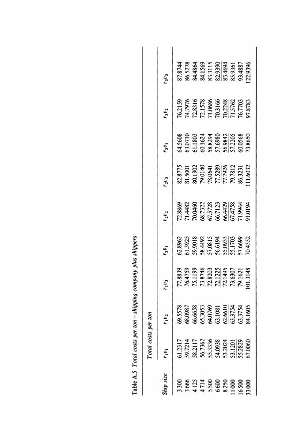
Tab
le A
.5
Tot
al c
osts
per
ton
-sh
ippi
ng c
ompa
ny p
lus
ship
pers
Tot
al c
osts
per
ton
Ship
siz
e r1
v 1
r 1v 2
r 1
v 3
r 2v 1
r 2
v 2
r 2v 3
r 3
v l
r 3v 2
r3
v 3
3300
61
.231
7 69
.557
8 77
.883
9 62
.896
2 72
.886
9 82
.877
5 64
.560
8 76
.215
9 87
.874
4 36
66
59.7
214
68.0
987
76.4
759
61.3
925
71.4
482
81.5
001
63.0
710
74.7
976
86.5
278
4125
58
.211
7 66
.665
8 75
.119
9 59
.901
8 70
.046
0 80
.190
2 61
.180
3 72
.831
6 84
.486
4 47
14
56.7
362
65.3
053
73.8
746
58.4
492
68.7
322
79.0
140
60.1
624
72.1
578
84.1
569
5500
55
.333
6 64
.076
9 72
.820
3 57
.081
5 67
.572
8 78
.064
1 58
.829
4 71
.068
6 83
.311
5 66
00
54.0
938
63.1
081
72.1
225
56.6
194
66.7
123
77.5
289
57.6
980
70.3
166
82.9
390
8250
53
.202
4 62
.661
0 72
.149
5 55
.093
3 66
.442
9 77
.792
6 56
.984
2 70
.224
8 83
.469
4 11
000
53.1
201
63.3
754
73.6
307
55.1
703
67.4
758
79.7
812
57.2
205
71.5
762
85.9
361
1650
0 55
.282
9 63
.375
4 79
.162
1 57
.669
9 71
.994
4 86
.323
1 60
.056
8 76
.770
3 93
.488
7 33
000
67.0
060
84.1
605
101.
3148
70
.435
2 91
.019
4 11
1.60
32
73.8
650
97.8
783
122.
9396
8 Port costs and charges and the problem of shipping and port sub-optimizations
The technical progress in ports seems to be the strategic factor for the development both of ships and ports. No giant tankers and bulk carriers would appear on the seas unless a multiplication of the bulk-cargo handling capacity, and the boom in investments in deep-water facilities had occurred in the post-war period. The container revolution would likewise not have happened unless a great number of container ports had emerged almost 'over night' at the end of the 1960s.
The key characteristic of the relationship between the development of ship design and the development of port design is the interdependency. On one hand, improvements in the cargo-handling technique in ports has made new types of ships, and bigger ships profitable. On the other hand, the profound change in ship design thus induced has, in turn, put new demands on the adjustments of the ports.
An individual shipowner takes the general development of ports, and an individual port authority takes the general development of ships as exogenously given from their different points of view. Nevertheless, the total effect on ports of shipowners' decisions about ship investment is of a most profound nature, and the same is true about the total effect on ships of port authorities decisions about port investment.
8.1 'PUBLIC' GENERAL CARGO TRANSPORT SYSTEMS VERSUS 'PRIVATE' BULK CARGO TRANSPORT SYSTEMS
In the analysis of the previous chapters of ship size and liner-service design we have treated shipowners' and shippers' costs and port charges equally. It is very pertinent to argue that the port charges should reflect the complete realport costs caused by ships of different type and size in order to attain a true optimum. In a 'closed system' context represented by, for example, some bulk transport systems where the ware owner is a shipowner and port owner as well, such a total-cost calculation is a matter of course. However, general cargo ports normally serve many different trades and shipping lines and numerous different shippers. And it is in fact impossible to devise a system of port charges which faithfully reflects investment costs caused by different ships without being in conflict with the aim of optimal use of existingfacilities. We argue that it is illusory to think that the port authorities could steer the ship-design development in an optimal way by exacting the full 'port cost responsibility'
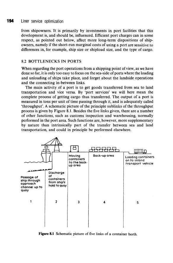
194 Liner service optimization
from shipowners. It is primarily by investments in port facilities that this development is, and should be, influenced. Efficient port charges can in some respect, as pointed out below, affect more long-term dispositions of shipowners, namely if the short-run marginal costs of using a port are sensitive to differences in, for example, ship size or shipload size, and the type of cargo.
8.2 BOTTLENECKS IN PORTS
When regarding the port operations from a shipping point of view, as we have done so far, it is only too easy to focus on the sea-side of ports where the loading and unloading of ships take place, and forget about the landside operations and the connecting in-between links.
The main activity of a port is to get goods transferred from sea to land transportation and vice versa. By 'port services' we will here mean the complete process of getting cargo thus transferred. The output of a port is measured in tons per unit of time passing through it, and is adequately called 'throughput'. A schematic picture of the principle sublinks of the throughput process is given by Figure 8.1. Besides the five links given, there are a number of other functions, such as customs inspection and warehousing, normally performed in the port area. Such functions are, however, more supplementary by nature than intrinsically part of the transfer between sea and land transportation, and could in principle be performed elsewhere.
Passage of ship through approach channel up to quay
Discharge of con~ainers from ship's hold to quay
2 3
Back-up area
4
Loading conroiners on to inland ~ransport vehicle
5
Figure 8.1 Schematic picture of five links of a container berth.
Port costs and charges 195
That the chain is as strong as its weakest link is an outworn phrase but nevertheless useful point of departure. In every activity which consists of distinguishable links it is generally desirable to seek to attain harmony in the sense that the capacity of each link is equal. When the potential capacity of one link has been increased relatively by some innovation or other, every effort ought to be devoted to the improvement of the other links of the chain, in order to realize the full potential of the original innovation. Technical developments should be so canalized that the rate of increase in 'strength' of each link of the chain is on average more or less the same. In the short term, however, disharmony may occur from time to time on account of the inevitable shortterm random occurrence of major innovations.
Containerization has meant a definite breaking of the bottleneck in seaborne general-cargo transport which has been prevailing for centuries -the stowage and unstowage of cargo in the ship's holds. The breaking of this bottleneck has had a far-reaching impact on the other links of the transport chain.
The container was the logical continuation of the trend towards bigger package units. It was an answer to several demands. By standardization of container dimensions, the multi-purpose conventional cranes could be replaced by specialized high-capacity container cranes. The loading/unloading capacity per crane-hour was as a result multiplied something like thirty times!
When two container cranes, and, as sometimes happens three container cranes at a time are working on a ship, the turnround time of a container ship is only about a tenth of the turnround time of a conventional liner loading/unloading the same quantity of cargo. RoRo methods of loading and unloading big standardized units constitute, for similar reasons, an equally dramatic improvement of the capacity per unit length of quay.
One would have thought that containerization should tip the balance in favour of direct transfer of cargo between sea and, in particular, rail inland transport, i.e. omitting transit storage. Each container constitutes a complete carload. Tallying should not be an impediment to continuous direct loading or unloading. However, this does not seem to have happened. Direct rail-to-ship transfer of containers is not considered practical since the train of cars would have to be continuously moved to bring the containers within reach of the cranes during loading and unloading.
8.2.1 Increasing demand for back-up space
Land requirements of container, RoRo and packaged timber (or other big unit load) berths are very much greater than of a conventional break-bulk berth. On the other hand, berth throughput is many times higher in the former case. The picture is therefore incomplete as long as the land requirement per throughput ton is not paid attention to. Typical (round) figures for the total
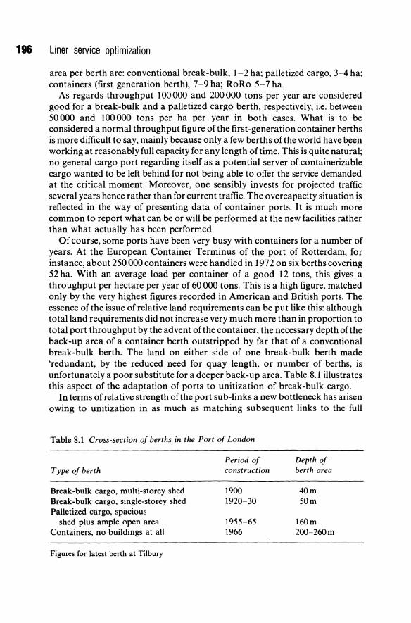
196 Liner service optimization
area per berth are: conventional break-bulk, 1-2 ha; palletized cargo, 3-4 ha; containers (first generation berth), 7-9 ha; RoRo 5-7 ha.
As regards throughput 100000 and 200000 tons per year are considered good for a break-bulk and a palletized cargo berth, respectively, i.e. between 50000 and 100000 tons per ha per year in both cases. What is to be considered a normal throughput figure of the first-generation container berths is more difficult to say, mainly because only a few berths of the world have b~en working at reasonably full capacity for any length oftime. This is quite natural; no general cargo port regarding itself as a potential server of containerizable cargo wanted to be left behind for not being able to offer the service demanded at the critical moment. Moreover, one sensibly invests for projected traffic several years hence rather than for current traffic. The overcapacity situation is reflected in the way of presenting data of container ports. It is much more common to report what can be or will be performed at the new facilities rather than what actually has been performed.
Of course, some ports have been very busy with containers for a number of years. At the European Container Terminus of the port of Rotterdam, for instance, about 250 000 containers were handled in 1972 on six berths covering 52 ha. With an average load per container of a good 12 tons, this gives a throughput per hectare per year of 60 000 tons. This is a high figure, matched only by the very highest figures recorded in American and British ports. The essence of the issue ofrelative land requirements can be put like this: although total land requirements did not increase very much more than in proportion to total port throughput by the advent of the container, the necessary depth of the back-up area of a container berth outstripped by far that of a conventional break-bulk berth. The land on either side of one break-bulk berth made 'redundant, by the reduced need for quay length, or number of berths, is unfortunately a poor substitute for a deeper back-up area. Table 8.1 illustrates this aspect of the adaptation of ports to unitization of break-bulk cargo.
In terms ofrelative strength of the port sub-links a new bottleneck has arisen owing to unitization in as much as matching subsequent links to the full
Table 8.1 Cross-section of berths in the Port of London
Type of berth
Break-bulk cargo, multi-storey shed Break-bulk cargo, single-storey shed Palletized cargo, spacious
shed plus ample open area Containers, no buildings at all
Figures for latest berth at Tilbury
Period of construction
1900 1920-30
1955-65 1966
Depth of berth area
40m 50m
160m 200-260m
Port costs and charges 197
potentials of the traditional bottlenek - the capacity to load and unload ships is next to impossible in ports designed for traditional break-bulk handling. What is needed more than anything else is supporting land for storage of containers in transit and to move them about in feeding the container cranes. In particular, if the obsolete finger-pier configuration still remains with hardly any back-up area at all except for some narrow - and, to make things worse, multi-storey - sheds, the problems of adaptation to the container age are very pressing. In addition, the water depth is insufficient in many older ports to accommodate the new bigger ships.
The problem is manifest in the tendency of ports to move out of town, down the river etc., to cheaper sites and deeper water. In some old ports, where cities have grown up around the port, this is the only economically feasible (although not always available) way out for the port. In San Francisco, for example, no site for a modern container port was available at the right moment, and as a result the containerizable business went across the San Francisco Bay from its historical port to Oakland, where appropriate land was plentiful. In New York City all major improvements to cargo piers on the Manhattan waterfront have been arrested. New facilities are located chiefly at Port Elisabeth, New Jersey. The development of the Port of London is a wellknown example of the need to build new berths further and further down the river estuary.
Second-generation container berths are built to comprise a paved area twice as large as the first-generation ones - about 16 ha instead of8 ha. The practical capacity of second-generation berths is, likewise, about twice that of firstgeneration berths, which leave throughput per hectare roughly unchanged. At least this is the picture that comes out from a comparison of the typical performance of first-generation berths with the highest throughputs reported so far at recently constructed berths. As was mentioned the practical capacity of the former is about 10000 tons per week per berth. This can be compared with some second-generation throughput 'records': at the four single-user berths of the Sealand terminal of Port Elisabeth a throughput equivalent to a good 20000 tons per berth per week has been achieved, and in the port of Oakland, the second-largest container port in the USA, the highest figure per berth amounted to about 26000 revenue tons per week at the beginning of the 1970s. In Japan the port of Kobe has recorded a container throughput at the Port Island C berth of about 30000 tons per week at the beginning of the 1980s.
8.2.2 The shipload size rather than the throughput volume determines the required back-up space
New containerships are getting bigger and bigger, and so are the shiploads of containers. Regardless, by and large, of the total throughput handled at the berth per year, space has to be provided which is at least proportional to the
198 Liner service optimization
size of the shipload. There are usually two resting areas for the containers, one close to the quayside and the other further away. The substantial additional area which is required for internal movements of the containers have to be considerably more than proportional to the shipload size for smooth and safe carriage of containers to and from the stacking area. This is a principal source of diseconomies of shipload size. As mentioned second-generation container berths are built to comprise a paved area twice as large as the first-generation berths. Where will this end? Still larger shiploads of containers to be handled at a time are anticipated. Deep-sea container ships of a carrying capacity around the equivalent of 2000 20-foot containers are now common. Still bigger ships are being put into operation on the longest liner-trade routes. The ScanDutch fleet of cellular container ships, for instance, which provide a service between Northern Europe and the Far East, have a capacity ranging from 2200 up to 2700 20-foot containers. It is rare that a whole shipload of containers of this size is loaded or unloaded in one port. The usual route pattern is that more than one port is called at at either end. The ScanDutch ships call at Gothenburg, Hamburg and Rotterdam in Europe and at Singapore, Kobe and Tokyo in the Far East.
It is expected, however, that the original idea of shuttle-services between pairs of central ports supplemented by feeder-services at either end will eventually come true. Consequently container-port authorities are preparing to cope with container flows coming intermittently in lumps of 2000 containers. Crane capacity is not a great problem; 2000 containers should be possible to load and unload in 30-80 hours depending on the number of cranes employed to achieve a reasonably quick turpround. The question is, however, how soon the next ship can be received? How quickly can a sufficient amount of the backup area be cleared so that another container 'avalanche' can be coped with.
Is the rapid increasing land requirement an inevitable consequence of the growth in size of container ships? Is it not possible to apply a less land-intensive technique of container handling in the ports? From American experience the following conclusion can be drawn. Two types of marshalling area designs are prevalent. In one, the containers remain on the trailer chassis with complete flexibility of movement. The container trailer combination is towed by the prime mover to an assigned location in the yard, remaining readily accessible for coupling to yard tractor for loading aboard ship. This method of operation requires more marshalling area than any other. The other system in common use requires block storage of the containers, usually two and sometimes three or even four high. Containers are placed by straddle carriers and may be rehandled a number of times before leaving the stackyard for good. In the case of export containers stacking height is not a great problem. Containers destined for a certain ship can and must be prestacked in the reverse order in which they will be loaded. As far as import containers are concerned, however, this land-saving method cannot be economically used to such an extent, because it is known exactly when the receivers will collect the containers.
Port costs and charges 199
Block storage minimizes the capital investment in rubber-tired chassis and land area but adds to yard operating costs and can cause delays in the loading and unloading of the ships.
The development of container terminals towards larger and larger 'plants' of higher and higher throughput capacity can be characterized as a process of 'breaking design bottlenecks'.
The meaning of a design bottleneck is that in one link of the production chain pronounced diseconomies of further capacity expansion prevail, whereas, at least on average, economies of further capacity expansion are enjoyed in the other links. The second condition is crucial. The idea of breaking a bottleneck is that something is to be gained in other links by a greater total capacity of the plant. When this is no longer the case the addition of another plant is likely to be the best way of further increasing capacity.
The question is now, if the design of a modern container berth represents the final stage where all major bottlenecks are overcome. The characteristic low berth-occupancy rate is perhaps a sign that this stage is not yet reached. If the capacities oflinks 2-5 (see Fig. 8.1) could be enhanced there are still gains to be made in the form of higher berth-occupancy rates and still quicker turnround of ships.
8.2.3 Third-generation container ship and port design
Are there more economies of ship size to be reaped in the process of strengthening links 2-5? The appearance of VLCCs of up to 4400 TEUs, is a sign that this is the case as far as the at-sea ~osts of the shipping company are concerned. For port design this imposes a great burden on links 2-5 and will restrict the number of ports that can be called at, just for this reason. The proposed tailor-made container terminal operated by conveyor belts suggested by Meeusen (1971) and its counterpart super container ship design proposed by Rath (1973), have not been adopted. Rath in order to provide solutions to, (a) problems of longitudinal strength and torsion of open deck VLCC, and (b) the increase in crane cycle as the beam and depth of ship increase, suggested a new design of super container ships which would remedy these size disadvantages. This includes the reintroduction of completely closed decks, and the abandoning of the lift-onllift-off principle of container loading and unloading.
Horizontal stowage of containers by means of conveyor belts, would replace the conventional methods of handling containers. The ships would have no vertical cells but horizontal longitudinal lanes beside and above each other from the bow to the stern. The containers from the lower lanes would be moved to the higher lanes, and vice versa by elevators. Two lanes would be used for loading and unloading containers in a continuous stream. This should increase the handling speed quite considerably.
The container terminal has to be tailor-made to these ships to meet the
200 Liner service optimization
'systems integration' requirement. The conveyor belts would transport the containers in different directions to and from the ship. Computer-controlled overhead cranes would move the containers between the conveyor belts and the stacking bays, and also to and from rail cars and trucks.
Such a system has been proposed by the consulting engineer, Meeusen (1971) for the layout of the Rijnpoort container terminal of the Port of Rotterdam. The terminal is planned to handle ultimately no less than the equivalence of 1.5 million 40-foot containers per year. The salient feature of the proposal is that on the seaside of the giant terminal the inlet and outlet for the ocean-going traffic is confined to the two conveyor belts moving containers in and out of a super container ship.
The proposed layout is interesting in the present context in that in its final shape it represents the theoretical extreme endpoint of the capacity-deepening era of the development of general-cargo port design. The terminal can be regarded as one giant berth with a twenty times greater throughput than the throughput of an existing berth. Although a huge back-up area is required the productivity per cubic metre in envisaged to be about three times higher than current performances with regard to container throughput per unit of berth area. In this sense the proposal, if it will be realized, represents a breaking of the prevailing bottleneck - the land hunger of the handling operations on the back-up area. The complete automation of these operations will allegedly cure this to a large extent.
Rath's (1973) and Meeusen's (1971) ideas have not been adopted by the industry. The new VLCCs are open-deck container ships and are handled by lift-on/lift-off cranes in ports, with the main difference that four to six cranes rather than two are being employed. The bottlenecks that will be created in links 2-5 and the way of coping with these are issues the industry will have to face, in the future.
8.3 PORT CHARGES AS A MEANS OF COORDINATING SHIPPING AND PORT OPERATIONS
One question which springs to mind when bigger and more specialized ships and ports are built is: Whoever can afford the risk of investing a super berth which requires super container ships to be profitable, or in a super container ship which requires super berths? No one is likely to venture such an investment unless assurance is given that the complementary factors are available.
Against this background the strong tendency to vertical integration in general-cargo transport which has been noticeable in the wake of containerization is not surprising. A similar means to the same end is the more-and-morecommon practice that ports investing in container berths attempt to have the shipping line(s) share the risk by binding up the user(s) by long-term hire contracts before the investments are carried out. Many shipping lines
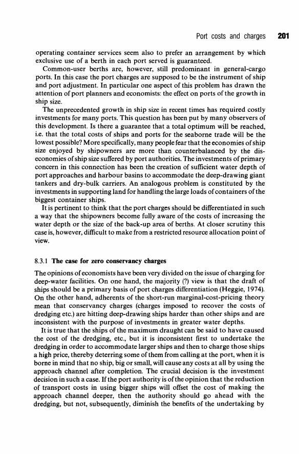
Port costs and charges 201
operating container services seem also to prefer an arrangement by which exclusive use of a berth in each port served is guaranteed.
Common-user berths are, however, still predominant in general-cargo ports. In this case the port charges are supposed to be the instrument of ship and port adjustment. In particular one aspect of this problem has drawn the attention of port planners and economists: the effect on ports of the growth in ship size.
The unprecedented growth in ship size in recent times has required costly investments for many ports. This question has been put by many observers of this development. Is there a guarantee that a total optimum will be reached, i.e. that the total costs of ships and ports for the seaborne trade will be the lowest possible? More specifically, many people fear that the economies of ship size enjoyed by shipowners are more than counterbalanced by the diseconomies of ship size suffered by port authorities. The investments of primary concern in this connection has been the creation of sufficient water depth of port approaches and harbour basins to accommodate the deep-drawing giant tankers and dry-bulk carriers. An analogous problem is constituted by the investments in supporting land for handling the large loads of containers of the biggest container ships.
It is pertinent to think that the port charges should be differentiated in such a way that the shipowners become fully aware of the costs of increasing the water depth or the size of the back-up area of berths. At closer scrutiny this case is, however, difficult to make from a restricted resource allocation point of view.
8.3.1 The case for zero conservancy charges
The opinions of economists have been very divided on the issue of charging for deep-water facilities. On one hand, the majority (?) view is that the draft of ships should be a primary basis of port charges differentiation (Heggie, 1974). On the other hand, adherents of the short-run marginal-cost-pricing theory mean that conservancy charges (charges imposed to recover the costs of dredging etc.) are hitting deep-drawing ships harder than other ships and are inconsistent with the purpose of investments in greater water depths.
It is true that the ships of the maximum draught can be said to have caused the cost of the dredging, etc., but it is inconsistent first to undertake the dredging in order to accommodate larger ships and then to charge those ships a high price, thereby deterring some of them from calling at the port, when it is borne in mind that no ship, big or small, will cause any costs at all by using the approach channel after completion. The crucial decision is the investment decision in such a case. If the port authority is of the opinion that the reduction of transport costs in using bigger ships will offset the cost of making the approach channel deeper, then the authority should go ahead with the dredging, but not, subsequently, diminish the benefits of the undertaking by

202 Liner service optimization
charging for the use of the (then) costless approach channel. The case for a zero conservancy charge for the use of uncongested dredged approach channels, advocated by Goss (1968; p. 160) is an example of this principle (see also Bennathan and Walters, 1983). This is a principle of general validity. (For an excellent statement of the same principle applied to road investments to accommodate heavy traffic, see Walters (1968), especially chapter IV.) The extra cost of designing any service-rendering facility, whatever it may be, in order to accommodate customers with particular requirements, cannot justify special 'surcharges' unless the marginal costs of actually rendering the service do vary between customers. When this is not the case, it is true that a problem of equity arises. It may seem hard on the 'small one', and rather too favourable for the 'big one', that the latter shall pay no more than the former, in spite of the fact that the latter has caused a major part of the facility construction costs.
Those who have criticized the idea of zero conservancy charges from a purely resource allocation point of view seem to be particularly uneasy about the long-run effects of , subsidizing' deep-drawing ships. It is true that by such a policy of port charging shipowners contemplating investments in still bigger ships do not take the consequent port costs into account. The reply to this argument is simply that it is the port authority that should take both ship costs and port costs into account when investing in deeper water. The port authority cannot really, unfortunately some may think, pass over this responsibility to shipowners via the port charging system. * Port authorities should be leading and shipowners lagging. It is an illusion to think that ports are 'helpless victims' of an inevitable development of ship-size growth. A port authority who finds that an investment to accommodate bigger ships is not justified -that the port costs would exceed the expected benefits accruing to shipowners - should, of course, not make the investment out of sheer 'growthmania' or on some other irrational ground.
I t is true that from the point of view of an individual port the problem looks quite different. Who is leading, and who is lagging? A general impression is that many port authorities take a rather passive attitude in this matter, believing that the continuous ship-size growth is an inevitable fact oflife. They think that they are 'adjusting' to this development. It is, of course, an illusion to some extent. Every port that undertakes water deepening and investments in higher crane capacity contributes more or less to the growth in ship sizes, even
*To be sure, schemes can be imagined by which port authorities in unison place the responsibility entirely with the shipowners. For example, suppose that port authorities publish charges on ships which at present cannot be accommodated. Then they wait and see. If no ships more deep-drawing than present port water depths are built then there is no need for investment in deeper port waters. On the other hand, if a sufficient number of ships are ordered which will require deeper port waters, the required investments will be carried out. The problem of this scheme is, of course, that an individual shipowner will be very reluctant to be the first to take the risk of ordering a ship which may be impossible to use because no other, or too few other, shipowners follow his example for port authorities to consider it worthwhile to deepen their ports. A favourable development of ship sizes may never be realized under these circumstances.
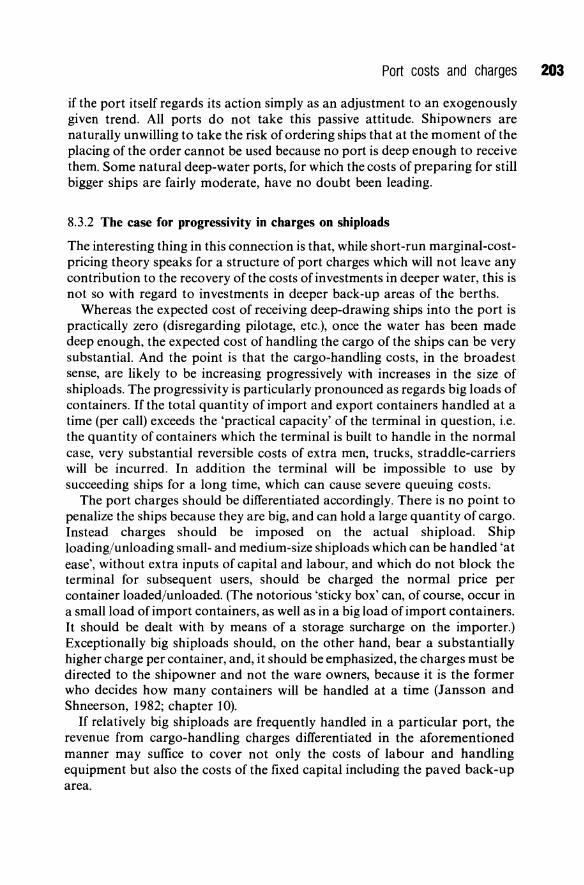
Port costs and charges 203
if the port itself regards its action simply as an adjustment to an exogenously given trend. All ports do not take this passive attitude. Shipowners are naturally unwilling to take the risk of ordering ships that at the moment of the placing of the order cannot be used because no port is deep enough to receive them. Some natural deep-water ports, for which the costs of preparing for still bigger ships are fairly moderate, have no doubt been leading.
8.3.2 The case for progressivity in charges on shiploads
The interesting thing in this connection is that, while short-run marginal-costpricing theory speaks for a structure of port charges which will not leave any contribution to the recovery of the costs of investments in deeper water, this is not so with regard to investments in deeper back-up areas of the berths.
Whereas the expected cost of receiving deep-drawing ships into the port is practically zero (disregarding pilotage, etc.), once the water has been made deep enough, the expected cost of handling the cargo of the ships can be very substantial. And the point is that the cargo-handling costs, in the broadest sense, are likely to be increasing progressively with increases in the size of shiploads. The progressivity is particularly pronounced as regards big loads of containers. If the total quantity of import and export containers handled at a time (per call) exceeds the 'practical capacity' of the terminal in question, i.e. the quantity of containers which the terminal is built to handle in the normal case, very substantial reversible costs of extra men, trucks, straddle-carriers will be incurred. In addition the terminal will be impossible to use by succeeding ships for a long time, which can cause severe queuing costs.
The port charges should be differentiated accordingly. There is no point to penalize the ships because they are big, and can hold a large quantity of cargo. Instead charges should be imposed on the actual shipload. Ship loading/unloading small- and medium-size shiploads which can be handled 'at ease', without extra inputs of capital and labour, and which do not block the terminal for subsequent users, should be charged the normal price per container loaded/unloaded. (The notorious 'sticky box' can, of course, occur in a small load of import containers, as well as in a big load of import containers. It should be dealt with by means of a storage surcharge on the importer.) Exceptionally big shiploads should, on the other hand, bear a substantially higher charge per container, and, it should be emphasized, the charges must be directed to the shipowner and not the ware owners, because it is the former who decides how many containers will be handled at a time (Jansson and Shneerson, 1982; chapter 10).
If relatively big shiploads are frequently handled in a particular port, the revenue from cargo-handling charges differentiated in the aforementioned manner may suffice to cover not only the costs of labour and handling equipment but also the costs of the fixed capital including the paved back-up area.
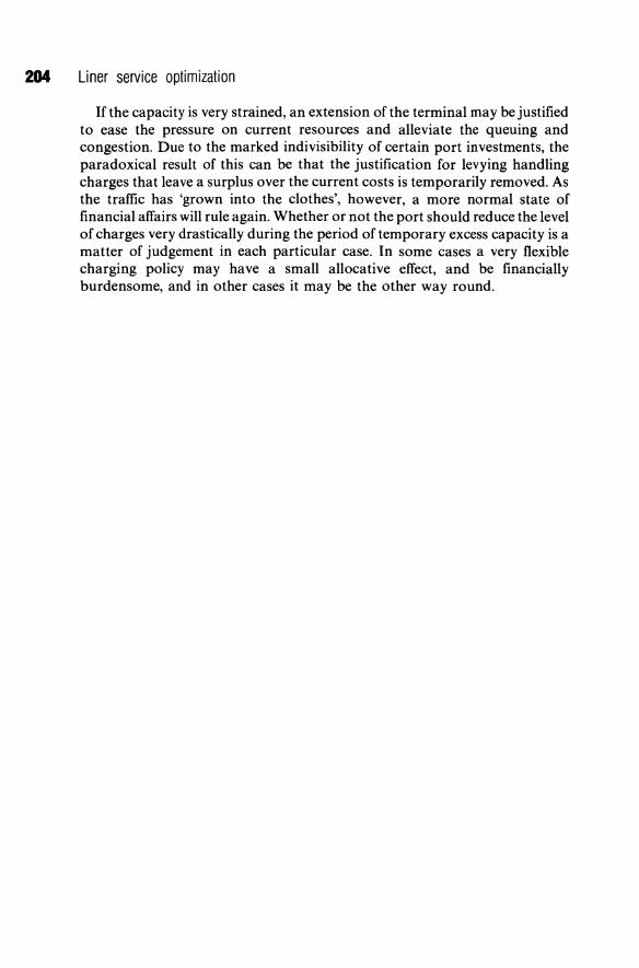
204 Liner service optimization
If the capacity is very strained, an extension of the terminal may be justified to ease the pressure on current resources and alleviate the queuing and congestion. Due to the marked indivisibility of certain port investments, the paradoxical result of this can be that the justification for levying handling charges that leave a surplus over the current costs is temporarily removed. As the traffic has 'grown into the clothes', however, a more normal state of financial affairs will rule again. Whether or not the port should reduce the level of charges very drastically during the period of temporary excess capacity is a matter of judgement in each particular case. In some cases a very flexible charging policy may have a small allocative effect, and be financially burdensome, and in other cases it may be the other way round.
9 A cost minimization model of a liner trade
9.1 A LINER TRADE MODEL - PURPOSE, SCOPE AND ASSUMPTION
The least-cost condition of servicing each level of output at the lowest possible cost per ton, should now be extended to include simultaneous determination of ship size, ports-of-call, and frequency.
The problem of designing liner services in thin trades is a problem of trading off shipping costs against costs of 'shipload consolidation in time and space'. To realize the shipping-cost economies of ship size in thin trades, full shiploads have to be gathered either by extending the cargo catchment, i.e. calling at more ports, or by increasing the intervals between sailings. Extending the cargo catchment area will result in higher shipping costs to the shipowner, and an increase in the interval between sailings will increase storage costs of shippers. The trade-off between the rise in these two cost categories and the fall in shipowners' costs as ship size increases, is at the heart of optimizing liner services in thin trades. The design ofliner services in thin trades should include simultaneous optimization of ship size, cargo catchment areas, and sailings frequency.
If substantial economies of scale exist, then liner services on thin routes may be out to compete with their non-schedule rivals. It would be interesting to study whether intercontinental liner shipping between Africa, South America, Southern Asia, Australia, Northern Europe etc., where the density of the general-cargo trade is relatively low, is at any great disadvantage as compared to liner shipping in the main trades of the world, or, in other words, whether significant economies of trade density exist in liner shipping. The fact that each particular market - liner trade - normally accommodates several shipping lines, suggests that these economies of scale are not marked. Second, the model should serve the shipping lines as a frame for optimizing their services to meet the objective of carrying the total cargo at the minimum costs per ton. The model, by its simplifying assumptions, cannot serve as a substitute to a detailed system-analysis approach that will have to be adopted in each specific case. It will help, though, to exemplify the directions of the effect of these variables when considered simultaneously.
The first question is to define the relevant markets, and this in turn will define the density of demand for a particular transport service. The model is adapted in the first place to intercontinental liner shipping. This implies, typically, that the trade between two opposite continental coasts, such as the Pacific coast of North America and East Asia (including Japan) or the west coast of Africa and the east coast of South America, constitutes the total

206 Liner service optimization
shipping demand of a particular market. The density of demand is then defined as the trade volume per kilometre of coast. This affords an admittedly imperfect demarcation of the system, unless clearcut geographical boundaries happen to exist as they do for liner shipping between Australia and New Zealand for example. In other cases some overlapping of markets is inevitable in reality, but there is no better alternative than to regard the different liner trades of the world as separate markets.
Another problem of system demarcation concerns the question of how far 'upstream' the cost analysis should be taken. In a narrow sense shipping service can be defined as the carriage of cargo from the quay of port A to the quay of port B. But more generally both the feeder transport costs (inland and sea) and the waiting costs should be included in the cost analysis of scheduled transport systems. In the present case this would mean that all the costs of transport - door-to-door and storage costs at the premises of consignors and consignees - should be taken into account. However, a departure from this general rule will be made in the following model. The ports of loading and discharge for each individual consignment will be treated as given. Under this condition, inland feeder-transport costs (to the port of loading and from the port of discharge) will be constant. Only feeder-transport operations undertaken by the liners themselves in the form of coastal diversions will be taken into account. Storage costs that are incurred either at the ports or at the consignors/consignee place, will be included in the cost model.
A third problem is that it cannot be assumed that one shipping line only serves each individual trade. However, in most trades the liner conferences act as a coordinating body. In the model it is assumed that the design of the shipping services fulfills the efficiency condition that each level of output is produced at the least total social costs. This is a necessary condition both for net social benefit maximization, and for total profit maximization. In other words, it is assumed that the liner conference/price cartel acts in accordance with the objective of maximizing the total profits of all members.
Given the above limitations and assumptions, the model is constructed as follows: consider the trade in general (liner) cargo between two continents separated by a sea; the problem is to design the liner-shipping services in such a way as to minimize the total social costs of transporting - in the widest sense -the total volume oftrade between a given number of ports - ml at one end, and m2 at the other. *
*The number of ports to be included in the services, "'1 and "'2 will be treated as given in the present model. Experiments with a more comprehensive model have shown that these design variables are only slightly dependent on the density of trade. Fixing values for"" and "'2 will not thus have much effect on the result regarding the magnitude of the economies of scale. The main determinants of Iii! and "'2 are the inland transport costs, and the transitional time of ships per call. There is little dependence only between"" and "'2 and the other design variables. The choice regarding ports-of-call is thus restricted to the question of how many of the given ports should be visited at each sailing. Needless to say, the different shipping lines should not call at the same subset of ports, but should divide the total market between them so that the conference most conveniently covers the whole trade.
A cost minimization model 207
The setting is homogenized in that the same quantity of cargo is assumed to be generated between each pair of ports. The total demand for shipping consists of the trade flows in both directions. Very few trades are well balanced. It is therefore appropriate to allow for an export-import imbalance (in measurement tons), and designate: total cargo flow, Q = X + M; 'export' (the trade flow on the fat leg), X = Q/p,; 'import' M = (1 - 1/p,)Q.
The measure of trade balance, p" assumes values between 1 and 2. The value ofthe lower limit indicates that the ships go in ballast in one direction, and the value of the upper limit indicates that the trade is perfectly balanced.
In spite of the fact that the ports served by the conference liners are given, the itineraries of the ships can be fixed in widely differing ways. At one extreme each ship could call at every port on each round voyage, which would require the maximum coastal diversion at each end, but which would also give the highest possibly frequency of sailings between each pair of ports (given the ship size). It is not necessary, of course, to call at every port on each round trip. Any number of ports-of-call between ml + m2 and two per round trip is possible. However, the fewer the ports-of-call, the lower will be the frequency of sailings between each pair of ports.
The other trade-off is between size and number of ships: given the itinerary of the ships, as the ships increase in size, so will the shipping cost per ton drop and the shippers' storage costs rise. Consequently, the design variables to be optimized are: number of round trips per year in the trade concerned, n; ship size, S; number of ports-of-call at one end per round trip, m l ; number of portsof-call at the other end, m2 ; frequency of sailings between each pair of ports, N.
Having discussed the shippers' costs of storage, and the feeder-transport costs, i.e. the costs of shipload consolidation in time and space, we are now in a better position to tackle the complete 'thin trade problem' of liner-service design.
Consider now the trade between two continents. Each coastline is divided into a number of ports generating an equal amount of cargo. The exports from each port to any other port on the other side is X, and the corresponding import volume is (p, - 1)X, when p, is the trade balance. (The ratio of total cargo volume to that of the fat leg.) ml is the number of ports on one end of the route, m2 is the number of ports at the other end. The total intercontinental trade is then = Xm l m2 . The maximum number of separate liner services is m l m2' implying shuttle services between each pair of ports. The trade density, X, has obviously to be very great indeed to warrant this pattern. It is most likely that each service should include a number of ports at each end. The question is how many for an optimum? We will answer this with a model that includes both producers' and users' costs.
9.2 TOTAL PRODUCER AND USER COSTS
The shipping costs directly borne by the shipowners are grouped into, (a) those costs which are time-proportional and incurred all the time, i.e. crew and

208 Liner service optimization
capital costs, (b) fuel costs which are incurred only during hauling time, which is proportional to the sailing distance, and (c) berth occupancy charges which are assumed to be time-proportional, and which are, of course, incurred only in port. The annual total costs of the first group are thus proportional to the product of the total number of round voyages, n, and the round voyage time, T; the total fuel costs are proportional to the total miles sailed by all ships, nD; and the total port charges are proportional to the total port time of all ships, which is equal to twice (loading and unloading) the total trade flow, Q, divided by the handling capacity, H, which - given the port productivity - is a function of the ship size.
The total costs of the shipping lines engaged in the trade can thus be written:
TCprod = nTUl(S) + fz(S)] + nDf3(S) + ;lZS/4(S) (9.1)
where the round trip time is
D 2Q T = V(S) + (ml + mz)h + nH l(S)" (9.2)
The three components of the round-trip time are from left to right, the total hauling time at sea, the total transitional time (h = transitional time per call), and the total time in port.
The round-trip distance is made up of two sea-crossings and the coastal cruising at each end, the length of which depends on the number of ports-ofcall. Assuming for simplicity that the ports at each end are equidistant, the diversion necessary to call at another port is always equal to d. Designating the coast-to-coast distance, D, we thus have:
D = 2Do + (ml + mz - 2)d. (9.3)
For the shippers the total costs appear in the form of liner freight rates, certain port charges, inland transport costs, insurance and interest costs on cargo in transit, and storage costs. None of these cost items can be disregarded because they are relatively insignificant. However, given that for each individual shipment, the port of loading and discharge is always the nearest port served by liner shipping, the inland transport costs do not vary with the design variables of the model and need not be considered. The direct cargohandling costs, i.e. stevedoring charges, and port charges on cargo, are also constant, However, in this case the constancy represents an inherent characteristic of the costs concerned, and is not due to any limitation of the analysis; it would be a bit misleading to leave them out.
Bearing in mind that cargo-handling charges are paid for loading as well as unloading, the total direct handling costs are written:
Total cargo-handling costs = 2CoQ. (9.4)
The interest cost on cargo in transit is a size-dependent cost which can

A cost minimization model 209
generally be written as the product of the total input of ship-days per year in the trade multiplied by the interest cost of an average cargo per day.
Total interest costs on cargo in transit = nTJs(S).
The storage cost, finally, belongs to another category: this cost is a function of the frequency of sailings between each pair of ports, N. As in the case of cargo costs, it can be assumed that storage costs are incurred by both exporters and importers.
Total storage cost = 2C I (N) Q.
Summing up the costs borne by the shippers, we get the total user costs:
(9.5)
Apart from the level offreight rates and cargo costs, the questions of greatest concern to the shippers are apparently the frequency of sailings between each particular pair of ports and the transit time. In a given trade, the average frequency of sailings, N, is determined by the ship size and the number of portsof-call per round trip. The total number of ports at each end is mi and m2 ,
respectively. This means that there are mi m2 pairs of ports to be served. On each round trip, m i m2 pairs enjoy service. The average frequency of sailings is therefore equal to the total number of round trips per annum, n, multiplied by the ratio of mI m2 to mI m2 •
m I m2 Xm I m2 N = n-~ = ----=---==---
m1m2 cP SmI m2 (9.6)
where cP is the mean load factor (occupancy rate) on the export leg, and thus S is the practical holding capacity. Adding total producer costs according to equation (9.1) and total user costs according to equation (9.5), and dividing by Q, gives us the following expression for the total social cost per ton:
_ nT nD 2 AC = 2Co + 2C I (F) + Q[fl (S) + f2(S) + fs(S)] + QJ3(S) + H I(S/4(S),
(9.7)
Inserting X/cPS for n, and the aforementioned expression (9.2) for T, and rearranging the terms, yields the following result:
AC = 2C + 2C(N) D[fI(S) + f2(S) + f3(S)V(S) + Js(S)] + IlcPSV(S)
(mi + m2)h[fl(S) + f2(S) + fs(S)] + IlcPS
(9.8)
2[f1 (S) + f2(S) + f4(S) + fs(S)] + HI (S) .
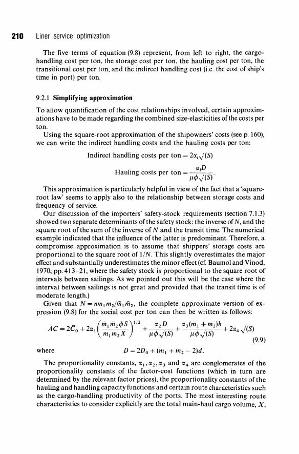
210 Liner service optimization
The five terms of equation (9.8) represent, from left to right, the cargohandling cost per ton, the storage cost per ton, the hauling cost per ton, the transitional cost per ton, and the indirect handling cost (i.e. the cost of ship's time in port) per ton.
9.2.1 Simplifying approximation
To allow quantification of the cost relationships involved, certain approximations have to be made regarding the combined size-elasticities ofthe costs per ton.
Using the square-root approximation of the shipowners' costs (see p. 160), we can write the indirect handling costs and the hauling costs per ton:
Indirect handling costs per ton = 2cx i .j(S)
H I· cxp au mg costs per ton = A. / .
J.1'f'y (S)
This approximation is particularly helpful in view of the fact that a 'squareroot law' seems to apply also to the relationship between storage costs and frequency of service.
Our discussion of the importers' safety-stock requirements (section 7.1.3) showed two separate determinants ofthe safety stock: the inverse of N, and the square root of the sum of the inverse of N and the transit time. The numerical example indicated that the influence of the latter is predominant. Therefore, a compromise approximation is to assume that shippers' storage costs are proportional to the square root of liN. This slightly overestimates the major effect and substantially underestimates the minor effect (cf. Baumol and Vinod, 1970; pp.413-21, where the safety stock is proportional to the square root of intervals between sailings. As we pointed out this will be the case where the interval between sailings is not great and provided that the transit time is of moderate length.)
Given that N = nm l m2 /m l m2 , the complete approximate version of expression (9.8) for the social cost per ton can then be written as follows:
- (mlm2<PS)l/2 cx2D cx3(ml + m2)h / AC = 2Co + 2cx l ml m2 X + J.1<P.j(S) + J.1<P.j(S) + 2cx4y (S)
(9.9)
where D = 2Do + (ml + m2 - 2)d.
The proportionality constants, CXl,CX2,CX3 and CX 4 are conglomerates of the proportionality constants of the factor-cost functions (which in turn are determined by the relevant factor prices), the proportionality constants of the hauling and handling capacity functions and certain route characteristics such as the cargo-handling productivity of the ports. The most interesting route characteristics to consider explicitly are the total main-haul cargo volume, X,
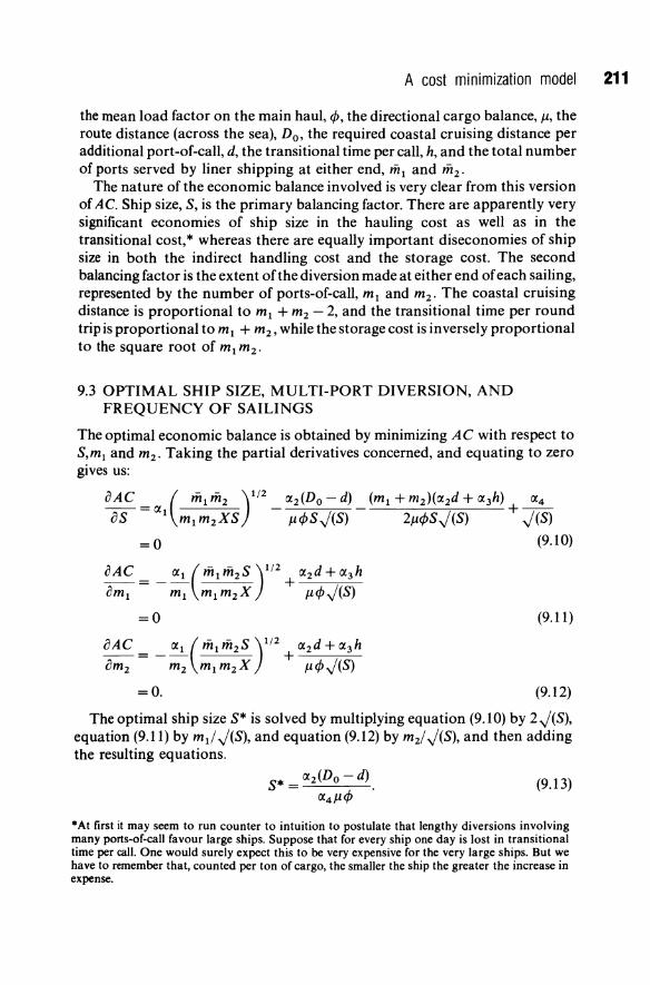
A cost minimization model 211
the mean load factor on the main haul, ¢, the directional cargo balance, f.l, the route distance (across the sea), Do, the required coastal cruising distance per additional port-of-call, d, the transitional time per call, h, and the total number of ports served by liner shipping at either end, ml and m2 •
The nature of the economic balance involved is very clear from this version of AC. Ship size, S, is the primary balancing factor. There are apparently very significant economies of ship size in the hauling cost as well as in the transitional cost, * whereas there are equally important diseconomies of ship size in both the indirect handling cost and the storage cost. The second balancing factor is the extent of the diversion made at either end of each sailing, represented by the number of ports-of-call, ml and m2. The coastal cruising distance is proportional to m l + m2 - 2, and the transitional time per round trip is proportional to m l + m2 , while the storage cost is inversely proportional to the square root of m l m2 .
9.3 OPTIMAL SHIP SIZE, MULTI-PORT DIVERSION, AND FREQUENCY OF SAILINGS
The optimal economic balance is obtained by minimizing AC with respect to S,m 1 and m2. Taking the partial derivatives concerned, and equating to zero gives us:
o AC = IX ( ml m2 )1/2 _ 1X2(Do - d) _ (ml + m2)(IX2d + 1X3h) ~ as I mlm2XS f.l¢SJ(S) 2wPSJ(s) + J(S)
= 0 (9.10)
oAC = _ ~(ml m2S )1/2 + 1X2d + 1X3h om l ml ml m2X f.l¢J(S)
=0 (9.11)
oAC = _ ~(ml m2S )1/2 + 1X2d + 1X3h om2 m2 ml m2X f.l¢J(S)
=0. (9.12)
The optimal ship size S* is solved by multiplying equation (9.10) by 2J(S), equation (9.11) by md J(S), and equation (9.12) by m2/ J(S), and then adding the resulting equations.
S* = 1X2(Do - d). 1X4f.l¢
(9.13)
·At first it may seem to run counter to intuition to postulate that lengthy diversions involving many ports-of-call favour large ships. Suppose that for every ship one day is lost in transitional time per call. One would surely expect this to be very expensive for the very large ships. But we have to remember that, counted per ton of cargo, the smaller the ship the greater the increase in expense.
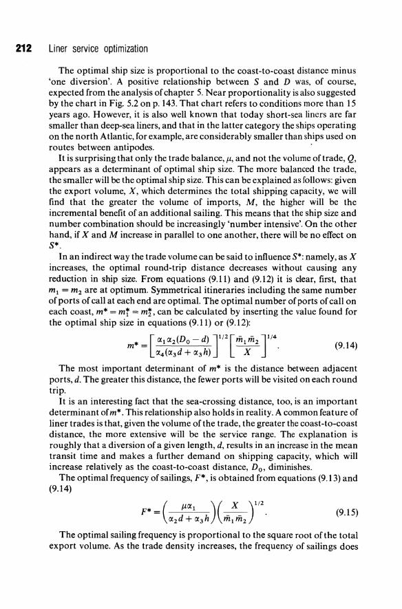
212 Liner service optimization
The optimal ship size is proportional to the coast-to-coast distance minus 'one diversion'. A positive relationship between Sand D was, of course, expected from the analysis of chapter 5. Near proportionality is also suggested by the chart in Fig. 5.2 on p. 143. That chart refers to conditions more than 15 years ago. However, it is also well known that today short-sea liners are far smaller than deep-sea liners, and that in the latter category the ships operating on the north Atlantic, for example, are considerably smaller than ships used on routes between antipodes.
It is surprising that only the trade balance, jJ., and not the volume of trade, Q, appears as a determinant of optimal ship size. The more balanced the trade, the smaller will be the optimal ship size. This can be explained as follows: given the export volume, X, which determines the total shipping capacity, we will find that the greater the volume of imports, M, the higher will be the incremental benefit of an additional sailing. This means that the ship size and number combination should be increasingly 'number intensive'. On the other hand, if X and M increase in parallel to one another, there will be no effect on S*.
In an indirect way the trade volume can be said to influence S*: namely, as X increases, the optimal round-trip distance decreases without causing any reduction in ship size. From equations (9.11) and (9.12) it is clear, first, that m1 = m2 are at optimum. Symmetrical itineraries including the same number of ports of call at each end are optimal. The optimal number of ports of call on each coast, m* = m! = m!, can be calculated by inserting the value found for the optimal ship size in equations (9.11) or (9.12):
m* = [Ct1 Ct2(Do - d) J1 /2 [m1 m2 J1 /4. Ct4 (Ct 3d + !X3h) X
(9.14)
The most important determinant of m* is the distance between adjacent ports, d. The greater this distance, the fewer ports will be visited on each round trip.
It is an interesting fact that the sea-crossing distance, too, is an important determinant ofm*. This relationship also holds in reality. A common feature of liner trades is that, given the volume ofthe trade, the greater the coast-to-coast distance, the more extensive will be the service range. The explanation is roughly that a diversion of a given length, d, results in an increase in the mean transit time and makes a further demand on shipping capacity, which will increase relatively as the coast-to-coast distance, Do, diminishes.
The optimal frequency of sailings, F*, is obtained from equations (9.13) and (9.14)
F* = ( jJ.Ct1 )(~)1/2 Ct 2 d+Ct3 h m 1 m2
(9.15)
The optimal sailing frequency is proportional to the square root of the total export volume. As the trade density increases, the frequency of sailings does
A cost minimization model 213
not increase commensurately; instead, the advantage of a greater trade volume is partly exploited by reducing the diversions caused by multiple calls at ports.
9.4 THE MINIMUM TOTAL COST PER TON
By inserting the values for S* and m* in equation (9.9), we obtain the total cost per ton at optimum. It is interesting coincidence that the total cost per ton is found to comprise, apart from the direct handling cost, two pairs of equal entities which can be identified as the storage cost (2C 1) and 'diversion cost' (2C 3 ::: the cost of coastal cruising and transitional time), on the one hand, and the sea-crossing cost (2C 2 ) and the indirect handling cost (2C4 ) on the other. (Note that each cost is incurred twice for each shipment.)
and
and
AC* = 2eo + 2CT + 2C! + 2C~ + 2C:
C* C* = [a2a4(Do - d)]1/4 2 + 4 11¢ .
(9.16)
(9.17)
(9.18)
Looking at equation (9.17), we can see that Q is a determinant of the storage and diversion costs. As we found previously, the frequency of sailings increase with increases in Q, but not fully in proportion to the increase in Q. A parallel effect is that the coastal diversions will be less extensive.
Looking at equation (9.18), we can observe that the trade volume is not a determinant of the sea-crossing and indirect handling costs. The reason as we have seen, is that the optimal ship size is independent of the trade volume. On the other hand, the trade balance, 11, has the effect of reducing these costs. So far as C! is concerned, a better trade balance does reduce costs, despite the fact that the optimal ship size falls with increases in 11. The economy of a higher overall load factor, however, is a stronger force.
What about the difference between the costs ofliner shipping in a thin trade and the costs in a trade where the density is ten or twenty times greater or even more? Equalizing the sea-crossing cost and diversion cost, letting this represent the extreme thin trade case and Q = co, C! = C~ = 0 represent the extreme dense trade case, the maximum ratio that can be expected of the cost of a thin route to the cost of a dense route (all factors except trade density being constant) appears to be about 5:3.
Needless to say, the factor prices contained in ai' a2' a3, and a4 are not the same all over the world. In reality we can therefore find many examples of higher costs in dense trades than in thin trades. Above all, the direct handling cost Co varies greatly from port to port. Cargo handling is particularly
214 Liner service optimization
expensive in American and Scandinavian ports. On the other hand, the indirect handling cost, C4 , is sometimes very high in many ports in low-wage countries, due to long queues. But these inter-trade differences are irrelevant in our present context. There is very little competition between liner shipping of different trades. Where it is relevant to compare costs, however, is between different forms of shipping in one and the same trade. Our purpose here has been to examine whether a low density of trade is likely to put liner shipping at any appreciable disadvantage in competition with tramp shipping and other possible forms of bulk services in which costs are commonly held to be largely independent of the trade density.
The conclusion is that a thin-route problem does exist in liner shipping, but that its gravity is not severe. In comparison to thin-route problem in public passenger transport, for example, it is quite minute.
9.4.1 Freight rates and distance
It is also interesting to note that the elasticity of C! with respect to coast to coast distance, Do, is as little as about O.S. A four-fold increase in the route distance will only double the sea-crossing cost. The total cost per ton is written:
AC* = 2eo + 4[C(1 (C(2 d + C(3 h)J1/2 (:~~ y/4 + 4[ C(2C(4~; - d) J/2
(9.19)
Since the total cost per ton, A C*, also contains the direct handling cost, the storage cost, and the diversion cost, which are all independent of Do, it follows that the elasticity of AC* with respect to Do is considerably less than the seacrossing cost elasticity. We can express the elasticity of AC* with respect to Do - d in this simple way:
[ AC* ][(Do - d)] C! (9.20) (Do-d) AC* =Co+C!+C!+C~+Cf
The distance elasticity of the total cost per ton is approximately equal to the share of the sea-crossing cost in the total cost per ton. As only the sea-crossing cost and indirect handling cost is increasing with distance, this elasticity is slightly increasing with distance. We have found that at optimum values the sea-crossing cost is equal to the indirect handling cost, and the storage cost is equal to the diversion cost; therefore one can give an interval of 0.17-0.3 as a likely range for the distance elasticity of the total cost per ton, where the lower value is applicable to short-sea trade routes, and the higher to deep-sea trades.
The freight rate comprises all these cost items except the storage cost, C 1.
Therefore, it is expected that the distance elasticity of the level offreight rates is to be found in the higher range. It is quite an interesting question, how liner freight rates in different trades vary with respect to route distance. The
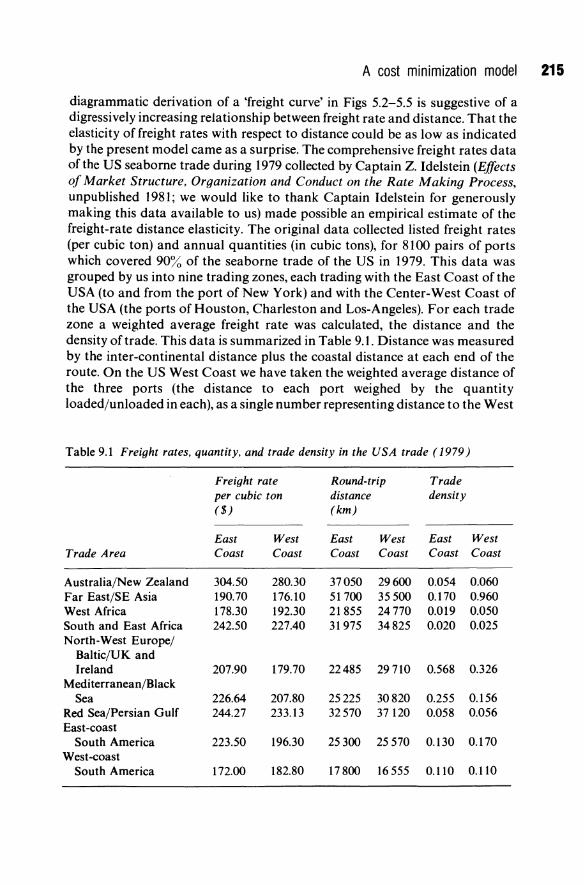
A cost minimization model 215
diagrammatic derivation of a 'freight curve' in Figs 5.2-5.5 is suggestive of a digressively increasing relationship between freight rate and distance. That the elasticity of freight rates with respect to distance could be as low as indicated by the present model came as a surprise. The comprehensive freight rates data of the US seaborne trade during 1979 collected by Captain Z. Idelstein (Effects of Market Structure. Organization and Conduct on the Rate Making Process, unpublished 1981; we would like to thank Captain Idelstein for generously making this data available to us) made possible an empirical estimate of the freight-rate distance elasticity. The original data collected listed freight rates (per cubic ton) and annual quantities (in cubic tons), for 8100 pairs of ports which covered 90% of the seaborne trade of the US in 1979. This data was grouped by us into nine trading zones, each trading with the East Coast of the USA (to and from the port of New York) and with the Center-West Coast of the USA (the ports of Houston, Charleston and Los-Angeles). For each trade zone a weighted average freight rate was calculated, the distance and the density of trade. This data is summarized in Table 9.1. Distance was measured by the inter-continental distance plus the coastal distance at each end of the route. On the US West Coast we have taken the weighted average distance of the three ports (the distance to each port weighed by the quantity loaded/unloaded in each), as a single number representing distance to the West
Table 9.1 Freight rates. quantity. and trade density in the USA trade (1979)
Freight rate Round-trip Trade per cubic ton distance density ($) (km)
East West East West East West Trade Area Coast Coast Coast Coast Coast Coast
Australia/New Zealand 304.50 280.30 37050 29600 0.054 0.060 Far East/SE Asia 190.70 176.10 51700 35500 0.l70 0.960 West Africa 178.30 192.30 21855 24770 0.019 0.050 South and East Africa 242.50 227.40 31975 34825 0.020 0.025 North-West Europe/
Baltic/UK and Ireland 207.90 179.70 22485 29710 0.568 0.326
Mediterranean/Black Sea 226.64 207.80 25225 30820 0.255 0.156
Red Sea/Persian Gulf 244.27 233.13 32570 37120 0.058 0.056 East-coast
South America 223.50 196.30 25300 25570 0.130 0.170 West-coast
South America 172.00 182.80 17800 16555 0.110 0.110
216 Liner service optimization
Coast. The trade density was measured by dividing the volume of trade by the coastal distance.
Given that the 'freight curve' tapers off, and the log relation was used in our system liner optimization, the relation between freight rates as dependent variable, distance and trade density as independent variables was estimated by a regression line of a log form:
log y = 2.940 + 0.223 log Xl - 0.056 log X 2
(2.260) (1.7 59) ( - 1.728)
(the figures in parentheses are the t statistics)
where: y = freight rate per cubic ton
Xl = distance in km
X 2 = trade density.
and jp =0.2 (9.21)
The regression results are in full support of the model's prediction. The freight-rate distance elasticity of 0.22 is within the range of 0.17~0.3 that the model predicted, just above the middle of this range. The freight-rate elasticity with respect to trade density is negative. Thus, the required freight rate declines with the intensity of demand, but very slightly so. The size elasticity is - 0.05. We may conclude on the basis of our model and the US evidence that distance as well as thin-trade routes are not very potent barriers to trade.
PART ECONOMIC EVALUATION OF THREE THE CONFERENCE SYSTEM
In this part we take up, at last, the controversial issue of the pricecartel organization of the liner shipping industry - the conference system. In the model of a liner trade in the previous chapter, we assumed that the shipping lines forming the conference in the trade could and should behave as a single unit when it comes to total system cost minimization. There we did not take up the revenue side. Now when it comes to pricing policy, an obvious question following from the preceding analysis is: why do not liner companies organized in liner conferences earn large monopoly profits? One part of the answer is that conference lines face competition from independent shipping lines in many trades, from the airlines who erode their high-value cargo, and from the tramps and neo-bulk services who compete for the minor bulk cargo. They are further constrained by shippers' councils, which can represent a significant countervailing power as compared to a large number of unorganized customers. On the other hand, the absence of supernormal profits should not necessarily be taken as a sign of health of the liner shipping industry implying that market performances are satisfactory. Our following discussion will show that this interpretation is incorrect.
We argue that the freight-rate making of liner conferences are obsolete. In the container age the continued practice of constructing detailed tariffs of commodity freight rates seems particularly archaic. More fundamentally, the more than lOO-year-old tradition of 'charging what the traffic can bear' has led to a generally low cost consciousness in the liner shipping industry: as will be demonstrated, the freight-rate structure is grossly out of line with the marginal cost of structure. The great disadvantage with the pricefixing power of the liner conference is that individual shipping companies, which, potentially, would like to pursue a more adequate, and innovative pricing policy than the more or less bureaucratic conferences, are easily tempted to adhere to established practices in exchange for a more quiet life attained by conference membership.
In line with our discussion in the previous chapter, we think that there is an economic rationale for coordination of the services
provided by individual shipping lines. Schedules and frequency are collective characteristics of liner markets. Shippers' costs depend on the services of all the lines collectively. In the absence of coordination of services, particularly in thin trades, the least-cost solution of the transport system would be difficult to obtain. Thus there is a raison d'etre for liner conferences. We envisage a new role for the conferences. They are needed not to prevent price competition, but to facilitate the coordination of sailings, ports of call, and possible sea-feeder transport services.
Before we make recommendations for change, it should be made clear exactly what is wrong with the pricing policy and practice of liner conferences.

10 The charging floor reconsidered
In chapters 3 and 4, it was shown that the freight-rate making by liner conferences is exceedingly simple so far as the underlying costing is concerned. It is basically a matter of establishing a 'charging floor' consisting of the direct handling costs. On the other hand, the determination of the appropriate contribution margin over and above the charging floor is a very elaborate exercise in the art of charging what the traffic can bear. It is a matter of coming as close as possible to the 'charging ceiling' of each commodity, without ever exceeding it.
We mean, and have argued so far over a decade (Jansson, 1974), that this pricing principle results in the freight-rate structure being grossly out of line with the corresponding marginal-cost structure. The main failure is that no shipping capacity limit is taken into account, and thereby a large volume of low-rated cargo is not paying its way, and large-scale cross-subsidization between commodities is taking place. This is not the only instance of crosssubsidization in liner shipping, but probably the most far-reaching form. We will take up other forms later on. To begin with we will concentrate on the question whether many low-rated commodities are carried at freight rates below their marginal costs. We mean that it is easily checked that this is so: take almost any liner trade, where a reasonable rate of capacity utilization obtains, and consider the withdrawal of, say one-third of the total number of ships in the trade, as well as one-third of the least-paying commodities. The result for the remaining ships would be a great rise in profitability.
This argument is not unchallenged (Gedda and Koch, 1966; Laing, 1975/76; Evans, 1977; Australian Department of Transport, 1977; Zerby and Conlon 1982). There are two lines of counter argument: one is that the disadvantage for the shippers of the remaining (high-rated) cargo of the lower frequency of sailings, that the capacity reduction would necessarily bring with it, is sufficiently great to offset the apparent gains ofthe shipowners, and another is that from the point of view of an individual shipping line the capacity costs of ships are common costs to all cargo carried, which cannot be allocated between commodities, each one of which comes in quantities well below what would be required to fill a ship. We take up these two arguments immediately under the headings of Economies of scale? and Common costs and factor indi visi bili ty.
10.1 ECONOMIES OF SCALE?
The former line of argument is an extension - which is entirely justified - of the ordinary concept of economies of scale in production to a total-system-
220 Economic evaluation of the conference system
cost context, where the producer (shipping line) costs and user (shipper) costs are treated as equal. If the sum of the costs of the shipping lines and the shippers per ton of cargo carried, is increasing with decreases in the total cargo volume, which is another way of saying that diseconomies of smaller-scale operations (i.e. economies of scale) apply, it may be true that the pricingrelevant marginal cost is as low as the current charging floor. This is not an either/or issue, which can be settled just by logic, but a matter of estimation of the cost relationship involved. Our model of a liner trade developed in the preceding chapter makes it possible to get an idea of how the total-system costs per ton are related to the total cargo volume in the trade, or 'trade density'. The relevant concept of 'scale' in this connection is the density of demand for shipping in the trade.
Before tackling the problem of economies of trade density, it is useful to make a distinction, discussed in the theoretical literature concerning externalities, and which is particularly relevant in the present context, namely, (a) economies of scale of a firm (shipping line), and (b) economies of scale of an industry (trade route). The former concept is relevant for questions of industrial concentration, and viability of competition.
Even if the firms of an industry are facing seemingly constant costs, it may be that the industry as a whole enjoys decreasing costs, as the total output of the industry is expanding. (The opposite case can also exist, i.e. increasing-cost industries consisting of constant-cost firms.) The economies of scale are then said to be external to the firms.
10.1.1 Economies of firm size
The relevant question to ask when it comes to possible economies of scale on the firm level is, what will happen to the unit cost of a representative firm if the firm will secure a large market share?
Significant economies of firm size are mostly to be found in industries consisting of single-plant firms. Economies of plant size and economies of firm size are then obviously synonymous. Multi-plant firms are presumably operating with plants of optimal size (at the time of construction of the plants), and the economies of scale in the production can be expected to be exhausted. Mergers of multi-plant firms can rarely be justified on production technological grounds, but marketing considerations, or simply a wish to restrict competition is the rationale. Shipping lines are multi-plant ( = ships) firms. A merger oftwo lines ofthe same conference is unlikely to result in any savings in shipping costs. The same number of ships will be plying the route concerned in much the same way as before. Of course, there is a possibility that savings in 'costs ashore' - overheads including the costs of general management and administration - can be achieved. A common experience is, however, that beliefs that savings in administrative costs can arise from agglomeration are largely illusory. That this is so also in liner shipping is supported by a crosssection analysis of a large number of shipping lines undertaken by Ferguson
The charging floor reconsidered 221
et al. (1961), which showed that the administrative costs amounted to about 10% of gross revenue regardless of the fleet size. A similar result is reported to have been reached in an investigation of USA shipping lines 10 years later (Devanney et al., 1972)
If there were unexploited economies offirms size in liner shipping one would expect that the number of shipping lines per trade are steadily falling. An attempt to examine whether a tendency towards concentration of lines on a route exists, was made at the same time by Ferguson et al. (1961). The case history studied by them failed to reveal any such tendency to concentration. The conclusion was that for ships on a deep-sea route further cost advantages of increasing the fleet size above four or five are doubtful. An upper limit of fifteen to twenty ships employed by one line (on anyone route under study) had been in existence for a long time.
The recent emergence of container service consortia in some trades is above all a reflection of the need to pool financial resources in order to adjust to a thoroughly changed technology. It may also imply that the smallest viable carrying capacity of a line has increased. The fact that a container ship normally replaces three or four conventional liners is important for the issue of economies of scale. So far containerization is concentrated to the densest routes of world trade. It is likely, however, that a tendency of ship sizes to grow faster than the liner business will spread to many other routes in the future.
10.1.2 Economies of trade density
When we move on to the industry level the issue of economies of scale appears in a somewhat different light. The relationship between the cost per ton - of users and producers - and the trade density on the route, i.e. the cargo flow per coastline kilometer at optimum in the previous model was (see p.213):
AC* = 2eo + 2CT + 2Ci + 2Cj + 2Ct
- +(mlm2)* [IXIIX2(Do - d)]+ = 2Co + 4[1X 1(1X 2d + 1X3h)] W/>Q + 4 fl.</> (10.1)
where Q is the total trade density, Co is the direct handling costs, ml , m2' Do, d, fl., </> and h are route characteristics, and lXI' 1X2' and 1X3 are constants.
The extent of the economies of scale can be measured by the elasticity of AC* with respect to Q. The first and third terms of AC* are apparently independent of Q, while the elasticity of the second term with respect to Q is equal to - 0.25. The overall elasticity thus depends on the ratio of the second term to the total cost per ton. This ratio falls as Q increases.
( 8AC*)( Q ) ( CT + Cj ) E = ----aQ AC* = - 0.25 Co + q + Ci + Cj + ct (10.2)
A more revealing expression for this elasticity can be obtained with the help
222 Economic evaluation of the conference system
of the equalities C! = C! and C! = Cl by considering the elasticity in terms of the direct handling cost, (Co), the sea-crossing cost, (C 2), and the diversion cost, (C 3)·
( 2C! ) E= -0.25 Co +2C!+2C! . (10.3)
A value of E almost as low as - 0.25 is clearly outside the realistic range. It would mean the diversion cost completely dominating the sea-crossing cost and the direct handling cost, which is never the case in reality. We can get a good idea of a realistic range of values for E by taking levels for the individual cost items which are typical of existing liner services. As has been mentioned, the service range at each end can embrace the coastline of a whole continent. Nevertheless, it is very unusual for the coastal diversion to be as long as the sea-crossing leg of a round trip because the really extensive service ranges are to be found only in connection with long-distance trade routes. It can also be shown that greater diversions (in relation to the coast-to-coast distance) are inefficient under most conditions. The increase in service frequency which will be attained is insufficient compensation for the additional shipping capacity required and the extending of the transit time.
In a short-sea trade the direct handling cost (stevedoring charges) is the dominating item. This means that neither C! nor C! is of an order of magnitude comparable to Co. In this case, the value of E barely differs from zero. In a deep-sea trade the sea-crossing cost and indirect handling cost (C! = Cl) can be on the level of the direct handling cost. A safe lower limit for the value of E under these conditions is obtained by setting Co = C! = C!. This gives us E = - 0.08.
The question is then how serious is the conflict between allocative efficiency and equity in liner shipping, given the inherent decreasing-cost character of this mode of transport. In other words: what level of freight rates can be expected in relation to the shipowners' average cost as a result of the application of the principle of (social) optimal pricing to liner shipping?
Setting freight rates equa~ to 'the average social cost of the marginal ship' and observing the conditions of design efficiency, we find that the total freight revenue falls short ofthe total shipping costs ( = shipowners' costs) by half the diversion cost. In other words, the optimal freight rate per ton of cargo, PC, is equal to the sum of the shipowners' costs per ton, except for the diversion cost at one end.
PC= 2(C! + Cn + C!. (10.4)
The optimal freight rate would fall short of the shipping cost per ton by about 0.2 at most. In relatively dense trades this fraction would be considerably smaller. For example if the total diversion cost at optimum is 0.3 of the sea-crossing cost, the discrepancy between the shipping cost and the optimal freight rate would only be 7% of the former.
The charging floor reconsidered 223
10.2 COMMON COST AND FACTOR INDIVISIBILITY
In discussions of liner shipping economics and policy the question of the optimal level of freight rates has not been much to the fore; nor should it be. Full cost pricing and optimal pricing would not produce very different results. However, in a multi-product enterprise like a shipping line another pseudoproblem ('pseudo' in our view) often looms large: How are the capacity costs to be allocated between different products using the capacity in common? To this problem we now turn.
The 'common cost' argument is, taken literally, simply fallacious. The ideas that the common capacity cost should be ignored in pricing disregards the basic notion of 'opportunity cost'. The opportunity cost of shipping capacity should not be zero on the fat leg in the normal case. When it happens to be zero, it is a signal to reduce capacity, and not to reduce the charging floor down to the level of the direct handling costs. After the appropriate capacity reduction (ship withdrawal) is made, it is time to set prices, and then, in a situation of supply and demand matching each other, the shadow price of capacity is far from zero. In an appendix to this chapter a model of profitmaximizing freight-rate making is presented, where the proper role of the opportunity cost of shipping capacity in costing and pricing is developed at some length.
When discussing the matter of the pricing-relevant marginal cost in shipping, it often turns out that the real problem is not that the shipping capacity cost is a common cost, but that a ship is an 'indivisible' factor of production, and, therefore, the capacity cost should not be included in the marginal cost. This is a general problem of 'part-load' transport markets, both for passengers and freight. When the 'part-loads' are relatively small- e.g. a single passenger on a busy bus carrying, say, sixty passengers, or a typical general-cargo consignment on a deep-sea liner - a problem of capacity indivisibility may appear. However, on routes where a reasonably large number of vehicles are engaged in a regular service, it seems that this problem has been exaggerated out of all proportion.
10.2.1 The average cost of a marginal vehicle
Where a marginal unit of capacity constitutes a relatively large capacity addition, a problem offactor indivisibility can arise. What decides whether it is a reasonable approximation to treat the number of least capacity units as a continuous variable, is not whether five, twenty-five or seventy-five passengers can be carried by an additional bus, or if 1000, 5000, or 25 000 tons of cargo can be carried by an additional liner ship; the crucial factor is rather the number of vehicles engaged on the route concerned. Treating this number as a continuous variable when calculating the pricing-relevant cost, is the same thing as approximating the marginal cost by the 'average cost of the marginal plant'. If there is only one plant serving a particular market, the average cost of
224 Economic evaluation of the conference system
an additional plant is certainly a poor marginal cost approximation in wide output intervals. If there had originally been 100 plant, it could have been a nearly perfect Me approximation. There is obviously no magic limit in this respect below which it can be deemed illegitimate to disregard factor indivisibility. Suffice it to say that, compared to other industries for which the 'average cost of the marginal plant' is a widely accepted approximation of the marginal cost, the production of transport services, where each vehicle corresponds to a separate plant, looks with few exceptions like quite a suitable area of application. This opinion seems not, however, to be generally approved of in the transport economics profession. There is a number of conceivable reasons for this.
10.2.2 Confusion of short-run marginal cost and average variable cost
First, the idea that capacity is a variable input in the pricing-relevant run for scheduled transport services of freight and passengers, is not - strangely enough - generally accepted by leading economists. However, operators of the services would be at a complete loss in the price-making, if they were to follow the recommendation that prices should be based on the short-run marginal costs, which, as illustrated in Fig. 10.1, are steeply rising as the capacity limit corresponding to each individual curve is approached:* Which short-run curve should be chosen as a match for the demand curve? Our answer is that, since pricing and capacity adjustment should be carried out simultaneously, a medium-run curve which, however, takes an entirely different path than the short-run ones, is the natural match for the demand curve. The failure by economists to point this out has led price-makers, in their bewilderment, to resort to the only firm ground in sight - the basically constant level ofthe direct handling costs. Therefore, low-value cargo thought to be unable to bear anything but very low charges are accepted for freight rates well below the pricing-relevant costs. The received costing principle, unfortunately, is to set the charging floor at the level of the handling cost.
Referring to Fig. 10.1, the result is that the 'wrong' (far too large) output is produced. As an interesting curiosity it can be mentioned that operators seldom make the mistake of equalizing capacity and expected demand. They are well aware of the fact that this would make the quality of service unacceptably low. A reasonable amount of reserve capacity is provided. Then a situation arises which seemingly justifies the chosen pricing policy; the ships usually sail with spare capacity: so was it not right to accept also low-paying cargo?
·In a realistic case where shipping demand shows substantial random variations from one sailing to another, the short-run marginal cost takes the smooth, although rapidly rising shape of Fig. 10.1, rather than the right-angled 'rigid capacity' shape that can be assumed in a deterministic demand model. The model in the appendix assumes a deterministic setting, but one point of the discussion there is that the basic conclusions will nevertheless be the same.
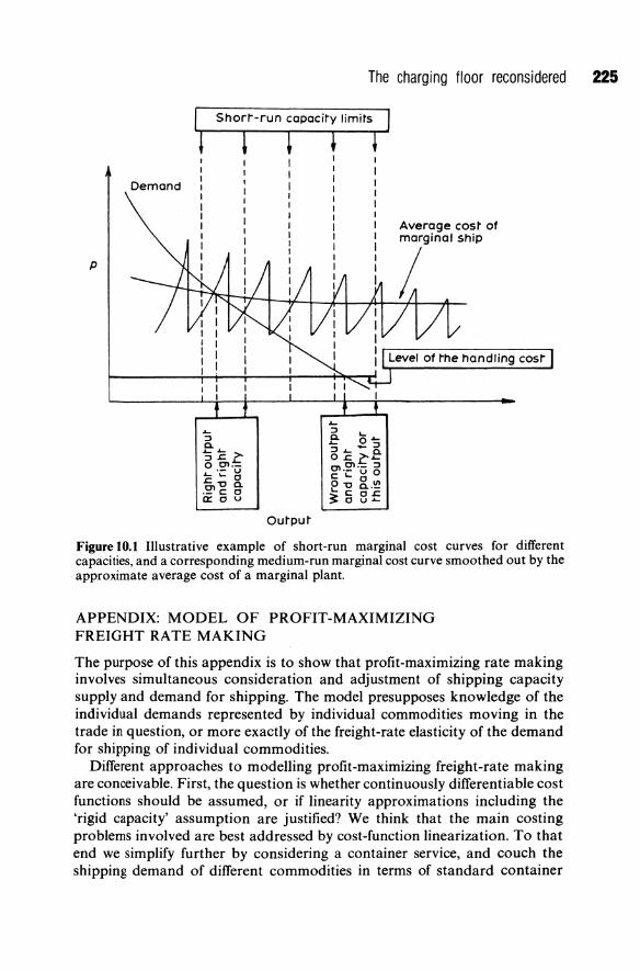
Demand
p
...... ::l a. 31::L" o 0'1._
.- u ........... 0 .g,"O a. ._ c: C 0: C u
Output
The charging floor reconsidered 225
Average cost of marginal ship
i
Figure 10.1 Illustrative example of short-run marginal cost curves for different capacities, and a corresponding medium-run marginal cost curve smoothed out by the approximate average cost of a marginal plant.
APPENDIX: MODEL OF PROFIT-MAXIMIZING FREIGHT RATE MAKING
The purpose of this appendix is to show that profit-maximizing rate making involves simultaneous consideration and adjustment of shipping capacity supply and demand for shipping. The model presupposes knowledge of the individual demands represented by individual commodities moving in the trade in question, or more exactly of the freight-rate elasticity of the demand for shipping of individual commodities.
Different approaches to modelling profit-maximizing freight-rate making are conceivable. First, the question is whether continuously differentiable cost functions should be assumed, or if linearity approximations including the 'rigid capacity' assumption are justified? We think that the main costing problems involved are best addressed by cost-function linearization. To that end we simplify further by considering a container service, and couch the shipping demand of different commodities in terms of standard container
226 Economic evaluation of the conference system
units. Thereby, we get rid of the notational problems posed in the case of break-bulk liner shipping.
Secondly, there is the eternal question of whether a short-run perspective is sufficient for discussing pricing, or if it is necessary to probe into a 'longer run'. For pedagogical reasons we start by couching the model in conventional short-run terms in order to make the eventual choice of a 'medium-run' approach self-evident.
A.l Profit maximization in the short run
In concord with established conventions, the short run is defined to imply that shipping capacity on the route is fixed. When it comes to scheduled liner services, it should mean that the schedule is given, too. In other words, we consider demand and supply of liner services with a planning horizon no further ahead than the current schedule is announced to apply. This can involve a period of time like the following 6, 9, or 12 months. For simplicity, let us assume that the current schedule ofliner services in the trade under study is fixed for exactly 1 year henceforth. This means in turn that we have to regard as an unalterable precondition for the freight-rate making that in the coming year: a given number of round voyages will be performed on the route; each ship has a given holding capacity; each round voyage is scheduled to take no more or no less than a given number of days. The freight rates to be fixed now should apply during the whole of next year like the schedule. This can be regarded as part of the service offered to shippers, but is also justified for reasons of practicability, especially under the present conditions when all freight-rate changes have to be approved by the liner conference. The possibility of selling out shipping services just before departure time when the cargo happens to fall well short of capacity is consequently conceivable only so far as open-rated cargo is concerned. Similarly, the possibility to raise freight rates to the market-clearing level each sailing when excess demand seems to occur is ruled out. Under these circumstances it is ill-advised to aim at 100% capacity utilization. Given that demand includes a significant stochastic element, optimum is obtained when the cargo volume on the fat leg equals the practical capacity, which is equal to the maximum capacity minus the spare capacity buffer required to offer a reasonable quality of service.
One has also to check that the total loading and unloading time requirement of the cargo one is planning to take on is not greater than is allowed for in the present schedule. The round voyage time is divisible into port time, cruising time at sea, and transition time between at-sea time and port time proper. With the present approach cruising time and transition time per round voyage is assumed to be given. Only port time is variable; port time proper is assumed to be proportional to the cargo volume handled.
For the same reason that makes a certain holding capacity reserve

The charging floor reconsidered 227
warranted, i.e. the stochastic element in demand, allowance should be made for a certain amount of reserve time. On average, the ship sails loaded to its practical capacity on the fat leg. Occasionally, however, a cargo larger than the practical capacity is lifted. Then more time is required for loading and unloading than the average port time requirement. This is taken into account by not letting the expected port time per round voyage be quite equal to the difference between the scheduled total round voyage time and the at-sea time plus transition time, but allowing for a certain amount of reserve time. Notionally we simply make the transition time constant A include also the reserve time per round voyage considered necessary.
The rate-making can consequently start by laying down the following constraints. We continue to adhere to the convention of naming the cargo on the fat leg 'export cargo'. Therefore we have:
The total volume of export cargo must not exceed the practical capacity, i.e.
x ~ n4>B. (A.t)
The total volume of import cargo must not exceed the practical capacity, i.e.
M~n4>B. (A.2)
The total time required for loading and unloading containers must not exceed the total scheduled round-voyage time minus total at-sea time and transition time including reserve time, i.e.
where
t(Q) ~ n( R - ~ - A )
x = export cargo lifted per year M = import cargo lifted per year Q = total (export + import) cargo lifted per year n = number of round voyages put in per year
(A.3)
B = 'bale' holding capacity of ships (maximum number of standard container units per ship)
4> = practical rate of holding capacity utilization t = gross loading and unloading time per container (including a
certain proportion of idle time) R = scheduled round-voyage time D = round-voyage distance V = cruising speed A = transition and reserve time.
Given these constraints the problem is now to maximize the net revenue by charging every commodity moving on each leg of the route individual freight rates. The cargo quantities (stuffed in containers) that will be forthcoming can, in principle, be regarded as functions of the freight rates. On the fat leg we have,
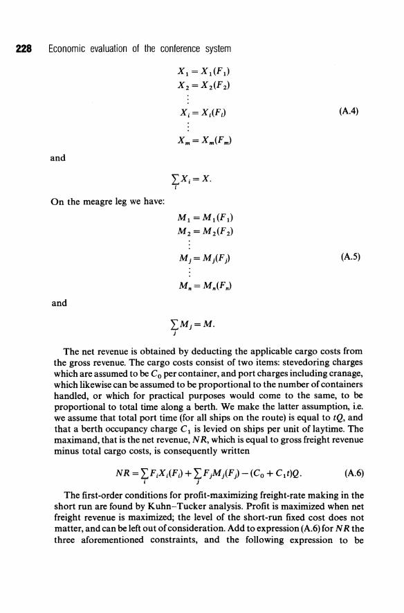
228 Economic evaluation of the conference system
and
On the meagre leg we have:
and
Xl =XI(FI)
X 2 =X2 (F 2 )
IXi=X. i
MI = MdF I )
M2 = M 2 (F2)
(AA)
(A.S)
The net revenue is obtained by deducting the applicable cargo costs from the gross revenue. The cargo costs consist of two items: stevedoring charges which are assumed to be Co per container, and port charges including cranage, which likewise can be assumed to be proportional to the number of containers handled, or which for practical purposes would come to the same, to be proportional to total time along a berth. We make the latter assumption, i.e. we assume that total port time (for all ships on the route) is equal to tQ, and that a berth occupancy charge C I is levied on ships per unit of lay time. The maximand, that is the net revenue, N R, which is equal to gross freight revenue minus total cargo costs, is consequently written
NR = I FiXi(Fi) + I FjMj(F) - (Co + Clt)Q. (A.6) i j
The first-order conditions for profit-maximizing freight-rate making in the short run are found by Kuhn-Tucker analysis. Profit is maximized when net freight revenue is maximized; the level of the short-run fixed cost does not matter, and can be left out of consideration. Add to expression (A.6) for N R the three aforementioned constraints, and the following expression to be
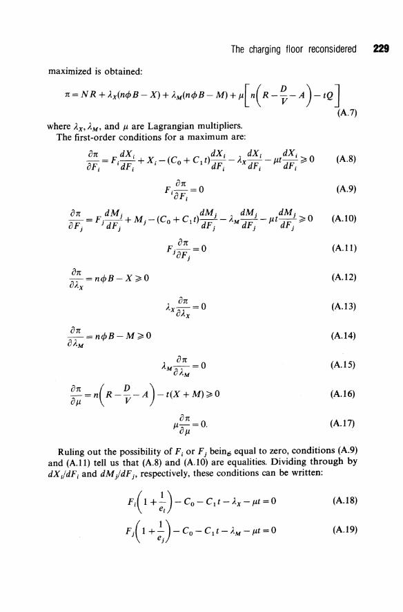
The charging floor reconsidered 229
maximized is obtained:
n=NR+Ax(n4>B-X)+AM(n4>B-M)+/{n(R- ~-A )-tQ ] where Ax, AM' and 11 are Lagrangian multipliers.
The first-order conditions for a maximum are:
on p.-=O
'oF;
on dM· dM· dM· dM· of. = F j dF ~ + M j - (Co + C 1 t) dF ~ - AM d/ - I1t dF ~ ~ 0
J J J J J
on F·-=O JoFj
an Ax OA = 0
x
on AM OAM = 0
an ( D ) -=n R---A -t(X +M)~O all v
on 11 011 = O.
(A. 7)
(A.8)
(A. 9)
(A. 10)
(A.ll)
(A.12)
(A. 13)
(A.14)
(A.15)
(A.16)
(A.17)
Ruling out the possibility of F; or F j bein6 equal to zero, conditions (A.9) and (A.1l) tell us that (A.8) and (A.1O) are equalities. Dividing through by dXJdF; and dM/dF j , respectively, these conditions can be written:
F{l + :J-CO-C1t-AX-l1t=O
Fj(l+ :J-CO-C1t-AM -l1t =O
(A.18)
(A.19)
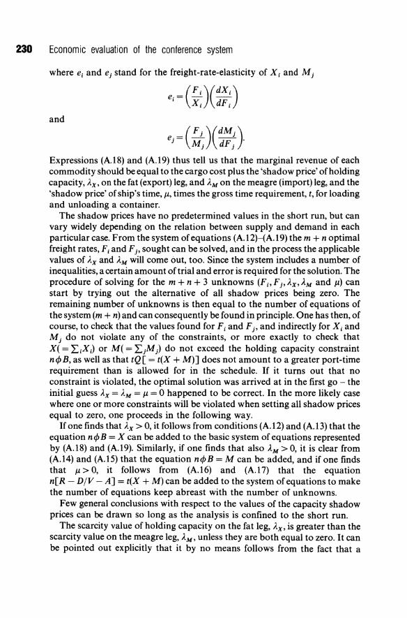
230 Economic evaluation of the conference system
where ei and ej stand for the freight-rate-elasticity of Xi and M j
ei=(Fi)(dXi) Xi dF i
and
. = (F j )(dMj ) eJ M· dF.· J J
Expressions (A.18) and (A.l9) thus tell us that the marginal revenue of each commodity should be equal to the cargo cost plus the 'shadow price' of holding capacity, Ax, on the fat (export) leg, and AM on the meagre (import) leg, and the 'shadow price' of ship's time, Il, times the gross time requirement, t, for loading and unloading a container.
The shadow prices have no predetermined values in the short run, but can vary widely depending on the relation between supply and demand in each particular case. From the system of equations (A. l2)-(A. 19) the m + n optimal freight rates, Fi and Fj, sought can be solved, and in the process the applicable values of Ax and AM will come out, too. Since the system includes a number of inequalities, a certain amount of trial and error is required for the solution. The procedure of solving for the m + n + 3 unknowns (Fi' Fj, Ax, AM and Il) can start by trying out the alternative of all shadow prices being zero. The remaining number of unknowns is then equal to the number of equations of the system (m + n) and can consequently be found in principle. One has then, of course, to check that the values found for Fi and Fj, and indirectly for Xi and M j do not violate any of the constraints, or more exactly to check that X( = LiXi) or M( = LjM) do not exceed the holding capacity constraint n¢B, as well as that tQ[ = t(X + M)] does not amount to a greater port-time requirement than is allowed for in the schedule. If it turns out that no constraint is violated, the optimal solution was arrived at in the first go - the initial guess AX = AM = Il = ° happened to be correct. In the more likely case where one or more constraints will be violated when setting all shadow prices equal to zero, one proceeds in the following way.
If one finds that Ax > 0, it follows from conditions (A.l2) and (A. 13) that the equation n¢B = X can be added to the basic system of equations represented by (A.l8) and (A.l9). Similarly, if one finds that also AM> 0, it is clear from (A.l4) and (A.l5) that the equation n¢B = M can be added, and if one finds that Il > 0, it follows from (A.l6) and (A.l7) that the equation n[R - D/V - A] = t(X + M) can be added to the system of equations to make the number of equations keep abreast with the number of unknowns.
Few general conclusions with respect to the values of the capacity shadow prices can be drawn so long as the analysis is confined to the short run.
The scarcity value of holding capacity on the fat leg, Ax, is greater than the scarcity value on the meagre leg, AM, unless they are both equal to zero. It can be pointed out explicitly that it by no means follows from the fact that a

The charging floor reconsidered 231
'meagre leg' can be identified that the associated capacity shadow price, AM, is necessarily equal to zero, or, which is the reflected image thereof, as can be seen from (A.14) and (A. IS), that the average load factor will be less than c/J on the meagre leg. If shipping capacity happens to be on the low side in relation to demand, and the difference in demand intensity between the two legs is not very marked, it may well be that the load factors should be the same, i.e. equal to ¢, implying full practical capacity utilization on both legs. The value of f.1. -
the scarcity value of ship's time - is equally indeterminate, a priori, as the values of Ax and AM in the present short-run setting. Two main cases are conceivable as is clear from (A.l7): either f.1. = 0 in which case the schedule includes so much reserve time that it never happens that cargo has to be rejected due to shortage of time, or f.1. > 0 in which case time is a scarce resource. If the schedule happens to be very tight it would frequently be necessary to decline to accept cargo in order to be able to keep the schedule. This could justify quite a substantial contribution margin on time-consuming articles in break-bulk cargo shipping - in a container service no freight-rate differentiation can, of course, be justified, on account of differences in handleability of individual articles inside the boxes. The main message is, however, addressed to those responsible for fixing the schedule. A very high value of f.1. is a sign that the schedule is too tight, and calls for a revision of the timetable rather than the freight-rate tariff.
More than anything else the present discussion should convey the feeling that the short run is not the right setting for freight-rate making. If an analysis of the preceding kind leads to the conclusion that Ax = AM = 0, and that the practical capacity will not be fully utilized in any direction, the right policy would not be to fix the freight rates in accordance with these conditions, bearing in mind that these freight rates have to apply at least for 1 year. The right policy is instead immediately to start adjusting the shipping capacity downwards, and then, or rather simultaneously, carry out the freight-rate making.
Similarly, if a short-run Kuhn-Tucker analysis reveals that the scarcity values Ax and AM are very high following a sudden jump in demand, let us say, the right policy is to adjust to this situation both by capacity additions and freight-rate adjustments. It seems clear that freight-rate making in liner shipping is a medium-run affair, and we now turn to the problem of profit maximization in the medium run.
A.2 Profit maximization in the medium run
In the medium run shipping capacity on the route concerned is variable. The shipping company(ies) operating there can vary the number of round voyages made on the route by re-allocating their ships between trade routes, by chartering in and chartering out ships, or even buying and selling ships. In addition to the cargo costs, the shipping costs proper, i.e. the costs of the ships

232 Economic evaluation of the conference system
themselves and their operation are variable costs in the medium run. On the assumption that ships of the same type and size are used, the shipping costs are by and large proportional to the total number of round trips put in on the route. A more detailed cost analysis calls for some modifications of that approximative relationship: it should be taken into account that the proportions of ships' time spent at sea and in port make a difference. The main items - ship capital and crew costs - are proportional to ship-time irrespective of how the time is spent, while the fuel costs are proportional to the total cruising distance (given the cruising speed) and the berth occupancy charges to the total time spent alongside a berth in port. We thus have the total cargo handling and shipping costs (TC) of the liners operating on the route as follows:
where
TC=Q(CO+c1t)+n[ Cz( A+ ~+t(;)+C3D ]
= Q[Co + t(C 1 + Cz)] + n[ C2 ( A + ~) + C3DJ
Co = stevedoring charges per container C 1 = port charges per unit of time of occupying a berth C2 = ship capital and crew cost per unit of time C3 = fuel cost per nautical mile.
(A.20)
The aforementioned three constraints change character when the medium run is considered. When capacity is a control variable a necessary condition for profit maximization is that full capacity utilization is obtained on the fat leg.
x = n<jJB. (A.la)
compared to (A.t) the inequality sign has been dropped. Capacity constraint (A.2), on the other hand, stands as it is, since it is not possible, a priori, to tell whether or not the capacity constraint should be binding on the meagre leg.
M ~ n<jJB. (A.2)
The third constraint implying that each round voyage must not exceed the scheduled time drops out, as the timetable determination is part of the medium-run demand and supply adjustment. In other words the unknowns to solve for now include the numbers of round trips put in per year, in addition to the freight rates F; and F j •
The relevant maxim and for profit maximization in the medium run is the difference between gross freight revenue and the total costs according to (A.20). Adding side-condition (A.la) and capacity constraint (A.2), the following expression to be maximized is obtained:
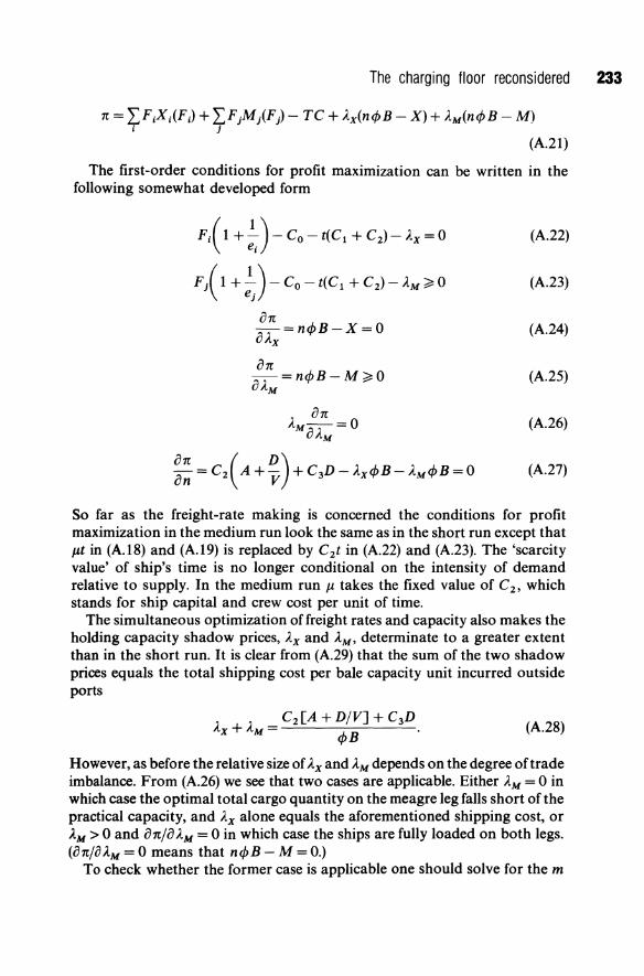
The charging floor reconsidered 233
n = 'L'piXi(Fi) + 'LFjMj(F) - TC + Ax(ncpB - X) + AM(ncpB - M) i j
(A.2I)
The first-order conditions for profit maximization can be written in the following somewhat developed form
F{ 1 +~)- Co - t(C1 + C2)- Ax =0
F j (l+ :J-Co-t(Cl+C2)-AM~0 on -=ncpB-X=O oAx
on oA =ncpB-M~O
M
(A.22)
(A.23)
(A.24)
(A.25)
(A.26)
(A.27)
So far as the freight-rate making is concerned the conditions for profit maximization in the medium run look the same as in the short run except that Jl.t in (A.18) and (A.19) is replaced by C2t in (A.22) and (A.23). The 'scarcity value' of ship's time is no longer conditional on the intensity of demand relative to supply. In the medium run Jl. takes the fixed value of C 2 , which stands for ship capital and crew cost per unit of time.
The simultaneous optimization offreight rates and capacity also makes the holding capacity shadow prices, Ax and AM, determinate to a greater extent than in the short run. It is clear from (A.29) that the sum of the two shadow prices equals the total shipping cost per bale capacity unit incurred outside ports
A A _ C2 [A + D/V] + C3D x + M - cpB . (A.28)
However, as before the relative size of Ax and AM depends on the degree oftrade imbalance. From (A.26) we see that two cases are applicable. Either AM = 0 in which case the optimal total cargo quantity on the meagre leg falls short of the practical capacity, and Ax alone equals the aforementioned shipping cost, or AM> 0 and on/oAM = 0 in which case the ships are fully loaded on both legs. (on/oA.M = 0 means that ncpB - M = 0.)
To check whether the former case is applicable one should solve for the m

234 Economic evaluation of the conference system
export freight rates in question, (F i ), on the assumption that
AX=[C2(A+~)+C3D J/<fJB and for the n import freight rates (Fj ) on the assumption that AM = O.
These freight rates yield in turn a set of (may be) optimal export cargo quantities X! ... xt .. . X:, and a set of (may be) optimal import cargo quantities M! ... Mj . .. M:. The check is then simply to add up all xt and all Mj to see whether the (may be) optimal total import cargo really is less than the (may be) optimal total export cargo. If one finds that M* > X* condition (A.27) is violated, since X* is equal to total practical capacity. In this event the second case is indicated, i.e. the case where AM > 0, and the optimal total cargo quantities on the two legs are equal. The optimal solution in the second case is obtained by the addition of the equality M* = X*, which makes the number of equations equal to the number of unknowns.
The basic character of the optimal solution in the second case is quite clear as far as the values of the shadow prices are concerned. When the trade is completely balanced
Ax=AM=t[ C2(A+~)+C3D J/<fJB. The more unbalanced it is, the larger the difference between Ax and AM will be. At a certain point AM becomes equal to zero, and the first case is applicable. How unbalanced the trade has to be in order for that case to apply is not possible to say in general. It depends on the freight-rate making elasticities of the individual commodities moving in the trade concerned.
A.2.1 Diagrammatic illustration
A diagrammatic illustration of the main point concerning the 'allocation,t of the n-proportional capacity costs between the fat and meagre legs is quite instructive. For expository reasons we have then to speak in aggregate terms: the curve designated NMRM in Fig. A.I represents the net marginal revenue for import cargo as a function of the total import cargo volume, and the curve designated NMR is the sum of the net marginal revenue of import and export cargo as a function of the total export cargo volume. The addition of 'net' before marginal revenue means that the cargo-proportional costs are deducted. Offered shipping capacity should be equal to the total export cargo volume. The optimal level of capacity is found where the marginal capacity cost - the Me-curve of Fig. A.1 - and NMR intersect. At that capacity level
tThis is, of course, a misleading term. One does not start by allocating total capacity costs between the two legs, but the profit maximization yields two capacity shadow prices, Ax and AM' the sum of which equals the capacity unit cost. The relative size of Ax and AM' however, is not predetermined.
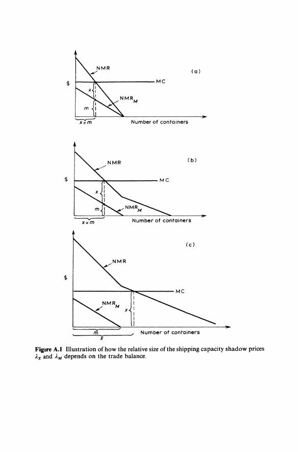
(a)
$ f--4.:--------- Me
Number of containers
( b)
$
Number of containers
$
Number of containers
Figure A.I Illustration of how the relative size ofthe shipping capacity shadow prices Ax and AM depends on the trade balance.
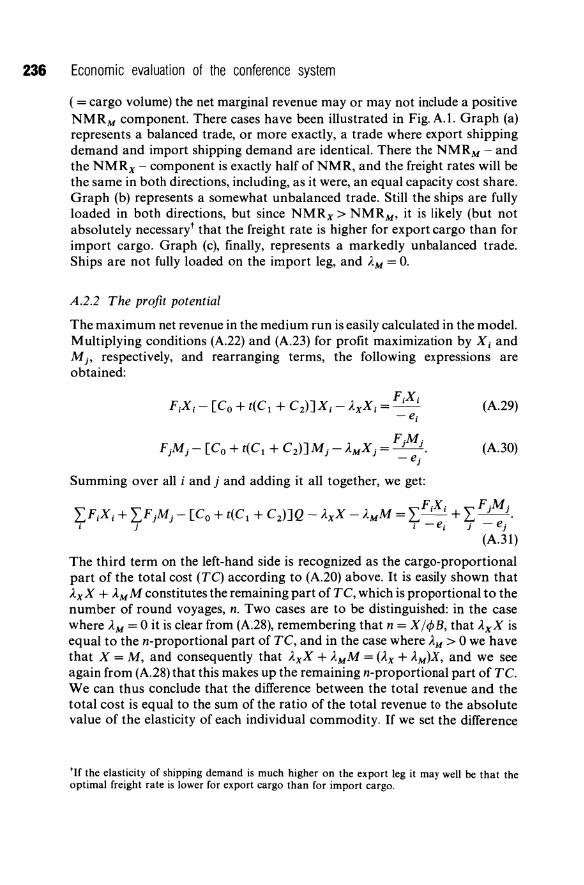
236 Economic evaluation of the conference system
( = cargo volume) the net marginal revenue mayor may not include a positive NMRM component. There cases have been illustrated in Fig. A.I. Graph (a) represents a balanced trade, or more exactly, a trade where export shipping demand and import shipping demand are identical. There the NMRM - and the NMRx - component is exactly half of NMR, and the freight rates will be the same in both directions, including, as it were, an equal capacity cost share. Graph (b) represents a somewhat unbalanced trade. Still the ships are fully loaded in both directions, but since NMRx > NMRM, it is likely (but not absolutely necessaryt that the freight rate is higher for export cargo than for import cargo. Graph (c), finally, represents a markedly unbalanced trade. Ships are not fully loaded on the import leg, and AM = O.
A.2.2 The profit potential
The maximum net revenue in the medium run is easily calculated in the model. Multiplying conditions (A.22) and (A.23) for profit maximization by Xi and M j' respectively, and rearranging terms, the following expressions are obtained:
(A.29)
(A. 30)
Summing over all i and j and adding it all together, we get:
F,x. F·M· 'LFiXi + 'LFjMj - [Co + t(C! + C2)]Q - AxX - AMM = 'L-'-' + 'L_J_l. i j i -ei j - ej
(A.31)
The third term on the left-hand side is recognized as the cargo-proportional part of the total cost (TC) according to (A.20) above. It is easily shown that AxX + AMM constitutes the remaining part of TC, which is proportional to the number of round voyages, n. Two cases are to be distinguished: in the case where AM = 0 it is clear from (A.28), remembering that n = X/<IJB, that AxX is equal to the n-proportional part of TC, and in the case where A.M > 0 we have that X = M, and consequently that AxX + AMM = (Ax + AM)X, and we see again from (A.28) that this makes up the remaining n-proportional part of TC. We can thus conclude that the difference between the total revenue and the total cost is equal to the sum of the ratio of the total revenue to the absolute value of the elasticity of each individual commodity. If we set the difference
tIf the elasticity of shipping demand is much higher on the export leg it may well be that the optimal freight rate is lower for export cargo than for import cargo.
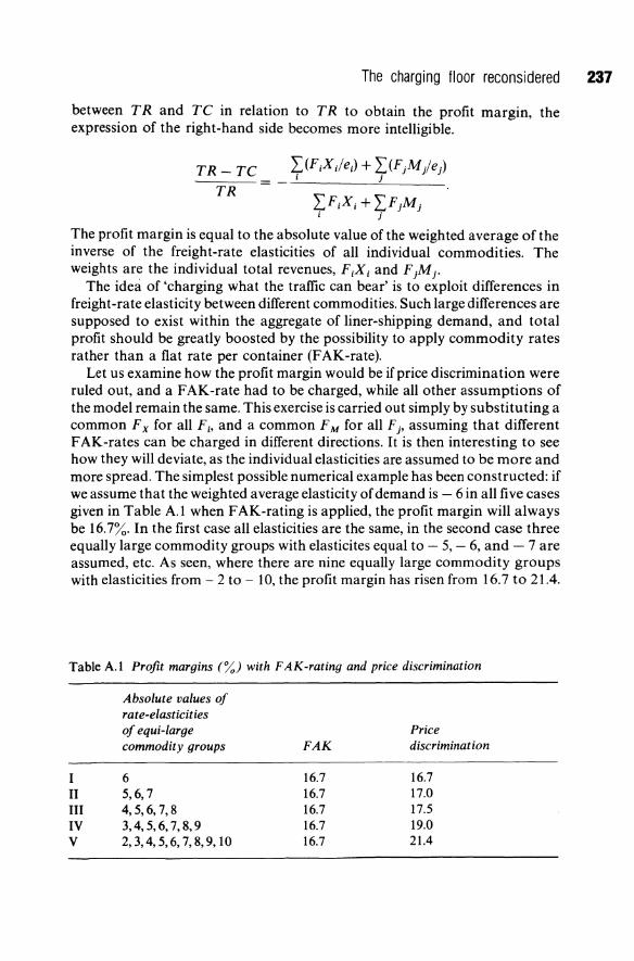
The charging floor reconsidered 237
between TR and TC in relation to TR to obtain the profit margin, the expression of the right-hand side becomes more intelligible.
TR-TC TR
~(FiXje;) + ~(FjM/ej) , }
IJiXi + L FjMj i j
The profit margin is equal to the absolute value of the weighted average of the inverse of the freight-rate elasticities of all individual commodities. The weights are the individual total revenues, FiXi and F .Mj.
, }
The idea of 'charging what the traffic can bear' is to exploit differences in freight-rate elasticity between different commodities. Such large differences are supposed to exist within the aggregate of liner-shipping demand, and total profit should be greatly boosted by the possibility to apply commodity rates rather than a flat rate per container (FAK-rate).
Let us examine how the profit margin would be if price discrimination were ruled out, and a FAK-rate had to be charged, while all other assumptions of the model remain the same. This exercise is carried out simply by substituting a common F x for all Fi> and a common F M for all Fj, assuming that different F AK-rates can be charged in different directions. It is then interesting to see how they will deviate, as the individual elasticities are assumed to be more and more spread. The simplest possible numerical example has been constructed: if we assume that the weighted average elasticity of demand is - 6 in all five cases given in Table A.l when FAK-rating is applied, the profit margin will always be 16.7%. In the first case all elasticities are the same, in the second case three equally large commodity groups with elasticites equal to - 5, - 6, and - 7 are assumed, etc. As seen, where there are nine equally large commodity groups with elasticities from - 2 to - 10, the profit margin has risen from 16.7 to 21.4.
Table A.1 Profit margins (%) with F AK-rating and price discrimination
Absolute values of rate-elasticities of equi-large Price commodity groups FAK discrimination
I 6 16.7 16.7 II 5,6,7 16.7 17.0 III 4,5,6,7,8 16.7 17.5 IV 3,4,5,6,7,8,9 16.7 19.0 V 2,3,4,5,6,7,8,9,10 16.7 21.4
11 The freight rate structure is out of line with the marg i nal cost structu re
In this chapter we will show in what respects, and to what extent actual freight rates deviate from the marginal costs. We start by outlining the costing principles which should underlie a cost-based tariff of freight rates, which will serve as the basis of comparison for the following examination of existing tariffs.
11.1 PRINCIPLES OF MARGINAL COST-BASED TARIFFS
In the demonstrated absence of appreciable economies of trade density, and excluding extremely thin and/or short-distance routes, a freight-rate tariff based on the marginal costs is quite a straightforward matter.
The objects offreight rates should be different packages including containers of specified sizes, or 'articles' which we use synonymously, rather than commodities. The package type and size is, however, not a sufficient specification of the articles of a marginal cost-based tariff.
The principal determinants of the marginal costs of shipping different articles are, the article 'handle ability', the ports of loading/unloading, the season when a shipment is sent, the shipment direction. For costing purposes the marginal cost of the kth article can conveniently be divided into, (a) a direct cargo-cost component, (b) an indirect handling-cost component, and (c) a hauling-cost component. The direct cargo cost consists primarily of stevedoring charges. The indirect handling costs are represented by lay time costs of ships in port.
Our investigation of the structure of break-bulk cargo handling costs (Jansson and Shneerson, 1982) indicates that a very substantial proportion of the variations in both the direct and indirect handling costs are explained by the package type, the package weight, and the stowage factor. The stowage factor is the ratio of package measurement (including broken stowage) to package weight. Alternatively the package measurement alone can be used (as a substitute for the stowage factor) as an article characteristic without reducing the explanatory power by much.
The applicable hauling costs can be regarded as the sum of, (a) the product of the bale capacity and the shadow price per unit of bale capacity, and (b) the product of the deadweight capacity requirement and the shadow price per unit of deadweight capacity. In a markedly unbalanced trade both holding capacity shadow prices are zero on the meagre leg, and on the fat leg the shadow price of deadweight capacity is zero in a pronounced 'measurement
The freight rate and marginal cost structure 239
trade', However, in less-clearcut cases the two shadow prices can take nonzero values on both legs on account of the possibilities that the normal capacity constraint can occasionally be reversed, so that ships may sometimes be loaded down before they are full.
11.2 CROSS-SUBSIDIZATION BETWEEN COMMODITIES
How much out ofline with the marginal cost structure are existing freight-rate structures? Immediately below we will give some examples of the degree of cross-subsidization between commodities, which is the main anomaly of present tariffs. In the next section we take up for discussion some other forms of cross-subsidization which have quite the opposite cause. The practice of 'averaging' of freight rates, ignoring a number of cost-influencing factors, implies too little differentiation with respect to port of loading and port of unloading, for example, and main-haul and back-haul cargo imbalance.
In previous work it has been shown on the basis offreight rate and cost data pertaining to US trades that 'intra-tariff cross-subsidization in liner shipping' (Jansson, 1974) was a salient feature in the 1960s, i.e. that on one and the same trade route, covered by one conference tariff, about half the cargo was moving at rates above the corresponding marginal costs, and the remaining cargo was moving at rates below the marginal costs. The rate-cost disparities were generally appreciable, and many examples of very substantial differences - both positive and negative - were found.
We have followed up this work, and here we will present some material which applies to a number of trade routes to and from Israel in the years of 1971-72. The level of freight rates and costs has doubled since those days. The freight-rate inflation has by and large been brought about by across-theboard rises, and there is nothing to suggest that freight rates of general cargo have become more in line with the marginal costs during this time.
The routes studied were in the Mediterranean trade on one hand, and in the trade with the USA, on the other. The latter trade includes two routes: the East Coast route, and the Gulf route. Comparisons of freight rates and costs were made for both conventional ships and container ships. The container ships were operating in the Mediterranean trade. The sample of commodities was taken from the applicable rate books. Commodities were selected on the basis of two criteria, (a) the importance in terms of their shares in the trade, and (b) for container ship - whether or not they were easily containerizable. Altogether, in consultation with the shipping lines operating on these routes, 473 freight rates of commodities being moved were compared to their costs.
The cost data were obtained from the accounts of the shipping companies. The data of the Mediterranean trade are from 1972; the data of the US trade are from 1971. The cost allocation has been greatly simplified by the fact that all trade routes under study are measurement trades, and that all two-leg routes are either markedly unbalanced, or, in some cases, nearly perfectly

300
250 (a)
200
150
100
50
50
100
(b)
500
400
300
200
100
50
50
450 (c)
400
300
200
100 50
50
100
Figure 11.1 (a) Percentage deviations of freight rates and marginal costs of Israeli imports in the US Atlantic trade. (b) Percentage deviations of freight rates and marginal

175
150
125
100
75
50
25
25
50
70 60 50 40 30 20 10
10 20 30 40 50 60 70 80
150
100
50
50
100
(d)
(el
~~~~~~~~~~~-
(f)
costs of Israeli exports in the US Atlantic trade. (c) Percentage deviations of freight rates and marginal costs of Israeli imports in the Mediterranean trade by conventional liners. (d) Israeli exports in the Mediterranean trade by conventional liners. (e) Israeli imports. in the Mediteranean trade by container ships. (f) Israeli exports in the Mediterranean trade by container-ships.

242 Economic evaluation of the conference system
balanced. In the US trade there was a marked excess of imports to Israel over exports. All at-sea costs, therefore, were allocated to the 'fat' inbound leg. In the Mediterranean trade the volume of export was approximately equal to the volume of import. In this case the hauling costs were divided equally between the two legs.
Direct handling costs were obtained from the tariffs of stevedoring charges. For the allocation of indirect handling costs we have used our results from previous studies of the influence on the handling performance of articles of different characteristics in American ports (Jansson and Shneerson, 1982). The use of these results for allocating indirect handling costs incurred also in Mediterranean ports, including Israeli ports, is, an approximation. We think that this is preferable to the alternative of not differentiating the indirect handling costs at all.
(a) The results
Lists of freight rates and marginal costs of commodities included in the sample are given as an appendix to this chapter. The charts below summarize the result of comparing the freight rates and the marginal costs. The six charts of Fig. l1.1(aHt) illustrate the percentage deviations of freight rates from the marginal costs. Each stem in the charts represents a percentage ratio of the difference between each freight rate and the applicable marginal cost to the marginal cost. For each particular route the values of these percentages are arranged in falling order (from left to right). Negative differences between freight rates and marginal costs are given by stems directed downwards.
The impression of widely disparate freight rates and marginal costs is very strong. As can be seen a general tendency is that the upwards disparities are on average larger than the downward disparities. (The negative difference between a freight rate and the marginal cost can, of course, not exceed 100% of the marginal cost, while no upper limit exists for positive differences.) This must not be interpreted to mean that the trades are necessarily very profitable. Each freight rate is represented by one stem irrespective of the volume of cargo carried. It can be safely guessed that the average quantity of commodities of the loss-making category is greater than the average quantity of commodities of the profit-making category.
11.3 EXCESSIVE AVERAGING OF FREIGHT RATES: SOME SUGGESTIONS FOR REFORMING THE TARIFF CONSTRUCTION
When looking at commodity freight rates the conclusion is that far too much differentiation is practiced. 'Commodity' is not a very valid cost factor. Examining existing freight-rate structures from other aspects, one finds too little freight-rate differentiation. Excessive averaging of freight rates is another

The freight rate and marginal cost structures 243
shortcoming in liner conference rate-making. We will now make some suggestions for adjusting freight rates more closely
to the marginal costs in a number of respects. We want to stress that this should not mean that tariffs become very complicated. One must be prepared to compromise between the desideratum of strict cost adherence and the desideratum of simplicity and lucidity of tariffs. To show this we start by discussing the more technical aspects of tariff construction, first for break-bulk cargo, and then for containers.
11.3.1 A cost-based tariff for break-bulk cargo
A linear form of the basic relationship between the shipping marginal costs of different articles and the article characteristics is:
(12.1)
where M C ijk = the marginal cost of shipping from the ith port to the jth port an article of the kth package type
rn = package measurement w = package weight
aijkrn = measurement-proportional cost component bijkW = weight-proportional cost component
Cijk = fixed cost per package unit (independent of package size).
In the common case where more than one port is called at in each service range the tariff construction will be somewhat involved in view of the likely possibility that some of the coefficients, aijk , and bijb and Cijk take different values for different ports for each given package type.
The technically most suitable tariff format would be a number of 'article matrices' of the kind shown by Fig. 11.2 with three entries for each pair of ports. One entry gives the charge per rn3, a second entry gives the charge per ton (1000 kg), and a third entry gives the fixed charge per package unit, which consequently is independent of the package size.
There have to be as many article matrices as there are package types. The most insignificant package types could perhaps be grouped together under a heading like 'general cargo, not otherwise specified'. In the example above we have suggested that a range of package weights is specified. An additional charge could be levied on exceptional units, both on unusually small and unusually big units, if there are good cost reasons for this.
More important is a peak and off-peak differential. The basic freight rates should be specified to apply to a period of time, e.g. the slack season. Outside this period one or more extra peak charges should be levied on top of the basic freight rates. Needless to say, the periods given in the example of Fig. 11.2 are entirely fictive. Finally, a quantity rebate may be justified. If this is the case, a simple way of making the freight rate of a given article taper off with increases
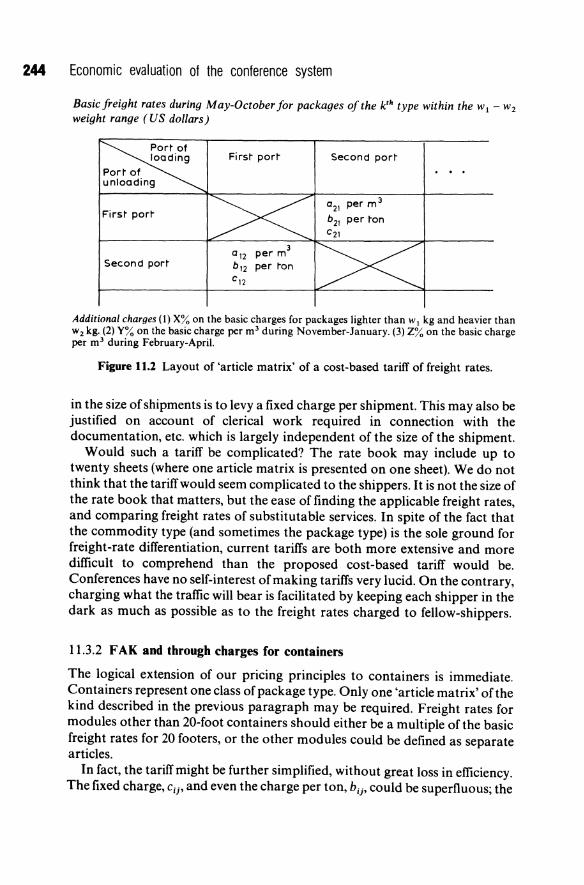
244 Economic evaluation of the conference system
Basicfreight rates during May-October for packages of the k'h type within the WI - w2
weight range (US dollars)
Port of loading
Port of unloading
First porr
Second port
Firsr porr
0 12 per m3
b 12 per ron c 12
Second porr
0 21 per m 3
b21 per ron C21
Additional charges (1) X% on the basic charges for packages lighter than WI kg and heavier than W 2 kg. (2) Y% on the basic charge per m3 during November-January. (3) Z% on the basic charge per m3 during February-April.
Figure 11.2 Layout of 'article matrix' of a cost-based tariff of freight rates.
in the size of shipments is to levy a fixed charge per shipment. This may also be justified on account of clerical work required in connection with the documentation, etc. which is largely independent of the size of the shipment.
Would such a tariff be complicated? The rate book may include up to twenty sheets (where one article matrix is presented on one sheet). We do not think that the tariff would seem complicated to the shippers. It is not the size of the rate book that matters, but the ease of finding the applicable freight rates, and comparing freight rates of substitutable services. In spite of the fact that the commodity type (and sometimes the package type) is the sole ground for freight-rate differentiation, current tariffs are both more extensive and more difficult to comprehend than the proposed cost-based tariff would be. Conferences have no self-interest of making tariffs very lucid. On the contrary, charging what the traffic will bear is facilitated by keeping each shipper in the dark as much as possible as to the freight rates charged to fellow-shippers.
11.3.2 F AK and through charges for containers
The logical extension of our pricing principles to containers is immediate. Containers represent one class of package type. Only one 'article matrix' of the kind described in the previous paragraph may be required. Freight rates for modules other than 20-foot containers should either be a multiple of the basic freight rates for 20 footers, or the other modules could be defined as separate articles.
In fact, the tariff might be further simplified, without great loss in efficiency. The fixed charge, cij ' and even the charge per ton, bij , could be superfluous; the

The freight rate and marginal cost structures 245
former because it would practically be identical to all containers, and the latter because for containerizable cargo, the effect of weight will be nil in most cases. The tariff would then have a single charge per cubic metre that will vary according to the ports of loading and unloading. And if a full container load is shipped, a single tariff per container that again will vary according to productivity in ports.
This is in fact the so called F AK rate ('freight of all kinds'). It has been contemplated as a substitute to the discriminatory structure of rates at the introductory stages of containerization, but has gained little ground since. Recently there has been a tendency for the shipping lines to offer container space to forwarding agents or other 'Non-vessel-operators' (NVOs) at F AK terms. The forwarding agents in their turn sell this space to individual shippers at a discriminatory structure of rates. This intermediate step is unnecessary and harmful. The shipping line can offer both a full-container load and a partcontainer load at F AK principles according to the scheme proposed here.
The appearance of containers in general-cargo shipping has raised some other tariff technical problems. Shipping lines have been anxious to keep the commodity rates (to make it possible to charge what the tariff can bear). This is obviously an aim which is in some conflict with the encouragement - on transport technical grounds - of 'through' container transports. If a container can be stuffed already at the premises of the consignor, and not stripped until it has reached its final destination, the maximum economy can be achieved.
The idea to match the door-to-door transport concept in the pricing policy was soon brought up. Whereas break-bulk freight rates have always applied to port-to-port (usually quay-to-quay, to be more exact) transports, an innovation in the wake of containerization was to offer all-inclusive, door-to-door freight rates. It would seem very natural to levy the 'through charges' per container. This would be the ultimate solution with regard to simplicity and efficiency. However, this has not happened. The wide freight-rate differentiation by commodities remains. Moreover, 'through charges' are difficult to apply with the present conference system, because inclusion of the feeder transport service in the freight rates gives individual conference members an opportunity to concede 'secret rebates' to shippers of the most coveted highrated cargo by subsidizing the feeder transport. This problem would disappear after the introduction of cost-based freight rates. Until recently another problem of liner conference through charges was that they were disallowed by US anti-trust laws. The inland part ofthe through transport was carried out by carriers not enjoying anti-trust immunity like the shipping lines, and therefore conferences were not permitted to fix through charges. This problem is now eliminated by the US Shipping Act, 1984. The new law clearly provided that conferences may lawfully receive authority from the Federal Maritime Commission (thereby receiving anti-trust immunity) for collective setting of intermodal through rates.
In a cost-based tariff of door-to-door container rates, points offreight origin
246 Economic evaluation of the conference system
and destination should replace the ports of loading and unloading. An accurately differentiated tariff could, however, be quite vast. The snag of a system ofthrough charges is that either the reflection of costs will be imperfect as to the inland transport costs, or the number of cargo generation and destination areas has to be quite large, which will make the tariff less handy. This snag can be avoided by giving up the idea of a single all-inclusive freight rate per container. The basic rate can instead cover just the port-to-port, or when applicable, the groupage depot-to-groupage depot transport. Such charges would anyway be required for container shippers who prefer to attend to the land transports themselves. A through charge would then consist of two components: the port-to-port rate and a charge which depends on the inland transport distance. Charges applicable to less-than-container-Ioad shippers who prefer to use possible pick-up/delivery services offered by the shipping lines would, similarly, consist of two components: a depot-to-depot basic charge and a distance-dependent additional charge. These charges can, of course, not be on a per-container basis but should apply to packages like break-bulk freight rates.
It is often held up as a disadvantage from a marketing point of view not to be able to quote a specific all-inclusive price for a specific through transport. Some proponents of door-to-door through charges seem prepared to disregard differences in inland location completely, and advocate the charging of just one single freight rate per container irrespective of the freight origin and destination as well as the ports ofloading and unloading. We can see no point in going to such an extreme for the sake of 'streamlining' freight-rate tariffs.
11.3.3 Abandonment of commodity freight rates and adoption of service classes
One radical difference between the type of our proposed freight-rate tariff and existing tariffs, which is worth emphasizing again, is that the type of commodity, which is the chief current freight-rate determinant is virtually irrelevant in our proposal. It is mainly in cases where commodities are handled in loose form that the commodity type is a principal cost factor. Packaged cargo is very dominating so far as liner shipping is concerned. Indirectly the type of commodity will playa role for the freight rates in so far that the measurement and weight of packages are influenced by the content. There may be some other intrinsic commodity qualities affecting the freight-rate structure.
Fragile commodities are more damage-prone and cause higher costs of claims than other commodities. If this fact is not reflected in the tariff, a source of controversy between shipper and shipowner emerges. Who should stand the risk of damage of fragile commodities? A fundamental principle is that, if the packing is inadequate the shipper should blame himself in case damages occur, and if the packing is adequate the carrier should regard it as his
The freight rate and marginal cost structures 247
responsibility to bring the shipment concerned safely to its destination. The problem is that it is very difficult to determine in every case what is adequate packing. The carrier can, of course, simply refuse to take on shipments of fragile commodities, which are clearly inadequately packaged. Borderline cases can, however, cause a lot of trouble. The goodwill of the shipping lines which frequently refuse shipments on account of inadequate packing will be damaged. A way out of this dilemma could be to introduce a class for 'fragile articles' in the tariff. Borderline cases (as to the packing of potentially fragile articles) need then not be refused, but classified as fragile articles. A freight-rate addition would compensate the carrier for the extra care that has to be devoted to fragile articles.
Other 'classes' can be envisaged, which on strict cost grounds would involve some degree of freight-rate differentiation between commodities. High-value commodities, and urgent (e.g. perishable) commodities would incur relatively high hauling costs. The idea of liner shipping is certainly to guarantee that space will be offered regularly, at pre-determined dates; but, as this guarantee cannot be regarded as absolute, some cargo will, from time to time, be left behind. At present, shipping lines apply a kind of implicit quality differentiation by a bookings policy which always gives priority to high-rated cargo on the occasions when demand exceeds supply. This is better done openly. A class for 'express shipments' could be established. Express shipments would never need to queue. A freight-rate addition is justified for express shipments, because such cargo causes extra capacity costs. At the other end of the scale a low 'stand-by rate' could be charged to shippers who are prepared to let their cargo always take the end position in the queue. Such cargo imposes obviously no queuing cost on other cargo, and causes little or no capacity costs.
11.4 FURTHER ASPECTS OF A COST-BASED FREIGHT RATE STRUCTURE
The cost-based tariff outlined above will look very different from the present liner conference tariffs. The question is, if the radical changes in the structure of freight rates will have any significant positive effects, i.e. if the pattern of seaborne trade and/or the allocation of resources for general-cargo transport will be significantly improved. It may well be that the seaborne trade that flows between each pair of trading areas will undergo only minor changes. The important effects will be on the arrangements of the transports of a by-andlarge given trade volume. The shipper's choice of type and size of break-bulk cargo packages and unit loads, and the seasonal timing of the shipments will be changed for the better. The distribution between the ports of call of the given volume of cargo in each particular trade will likewise be more efficient. Also the shipowners' choice of type and size of ships can be improved. Below we will develop in some more detail these effects of introducing a cost-based tariff of liner freight rates.
248 Economic evaluation of the conference system
11.4.1 Peak/off-peak redistribution of cargo
Given the annual trade volume on a particular route, there is, as a rule, considerable scope for redistribution in time of the trade flows, if only an incentive to do so is provided. In case there is a large difference between the average cargo flow per week during the peak season and that during off-peak, a redistribution of the cargo flow results in a seasonal levelling of the demand for shipping space would be very beneficial. The fleet size could be reduced proportionally to the decrease in peak demand. This will not be balanced by any need for additional ships during off-peak, because ships are then sailing with low load factors. The cost saving will not equal the whole of the possible reduction in shipping cost. The adjustment of the timing of trade flows is not costless. The main means of achieving a peak/off-peak redistribution of cargo flows is through additional storage. To arrive at the system cost savings of a peak/off-peak freight-rate differential the additional storage costs have to be deducted from the shipping-cost saving.
In liner shipping peak-load pricing has been very unusual on deep-sea routes, where the conference system is particularly well established. In shortsea shipping, at least so far as passenger services are concerned, price differentiation according to season is not unusual. A good example is the services between Gothenburg and Felixstowe, and Gothenburg and Amsterdam, which used to be run by Tor Lines, where the addition to the off-peak level of prices during the peak season is about 60%.
11.4.2 Optimal choice of type and size of break-bulk packages and unit loads
We have found in earlier investigations (Jansson and Shneerson, 1982) that tariffs of stevedoring charges for break-bulk cargo in the port of Rotterdam faithfully reflect the handling costs. This seems to be the case also in many other important ports. It is common that shipowners are major shareholders in stevedoring companies - Sweden is one example - and this tends to remove the temptation of charging what the traffic can bear on the part of stevedoring companies. To base the stevedoring tariffs on the handling costs seem to be regarded as the most equitable principle.
However, in order for cost-reflecting stevedoring charges to have any positive effects on the shipper's choice of package type and size a necessary condition is that the shipping lines pass on 'the message' from the stevedoring companies in an undistorted form. It is doubtful that this condition is generally fulfilled at the present time. Bearing in mind that the indirect handling costs are equally sensitive to the type and size of packages as the direct handling costs, a significant improvement in total efficiency could be made in the breakbulk cargo sector with regard to the packaging by introducing truly cost-based liner freight rates.
In the unit load sector the choice for the ware owners is highly restricted by
The freight rate and marginal cost structures 249
definition. The idea of unitization is, of course, that standardized loads are to be formed. So far the pattern has been that the ships that are employed in a particular liner service are either specialized unit-load carriers of a given type, or conventional liners. As was mentioned briefly in chapter 1 of current tendencies in general-cargo shipping, 'multi-purpose services' may well be an important part of the picture in the future. 'Flexibility' in the sense of ability to combine containers, trailers, and other unit loads as well as odd-shaped articles is a more-and-more common word of honour in liner shipping nowadays. Especially in the thin-trade sector it is a great advantage to offer a service which makes use of the whole potential cargo base rather than specializes on one category of cargo. The price mechanism has an important role to play in the evolution of multi-purpose services.
At present the most difficult aspect of introducing a container service into a certain trade is to evaluate the effects on shippers' costs of packaging, storage and feeder transport in a case where it is a matter of either/or. By adhering to the traditional principles of freight-rate making, operators of multi-purpose services will forfeit a golden opportunity to get valuable information about the shippers' costs and benefits of different general-cargo transport systems.
11.4.3 Premiums for efficient ports and outport surcharges
It is customary that liner conferences do not differentiate the freight rates of their tariffs with respect to ports within the service range. This practice has been rightly criticized. It fails to give an inducement to shippers to choose the most efficient port: with respect to the ports of loading and unloading, a differentiation of freight rates should be made not only on account of stevedoring charges that differ between ports, but also to reflect differences in the indirect handling costs, and expected waiting times.
There is another possible ground for differentiation offreight rates between ports, which is more complicated. If a particular port is awkwardly situated in relation to the rest of the ports, and, in addition, generates just a small quantity of cargo, it is a costly port to serve for the shipping lines regardless of stevedoring productivity and charges. The question is whether this is a rational ground for a freight-rate differential?
This type of question is a long-lived source of controversy between, on one hand, average cost-pricing proponents who think along 'cost responsibility' lines, and, on the other, marginal cost-pricing proponents. The recommendations ofthe two schools go widely apart. The total cost per ton, i.e. the average cost of the 'outport' is very high, whereas the marginal cost, i.e. the cost of another ton may seem rather low. The key point ofthe argument of economists of the marginal cost-pricing school is that this issue is by nature an investment problem in the first place. The question whether or not a particular port is to be included in the service should be answered by weighing the total separable cost against the total separable benefits. Once a decision is taken to include the
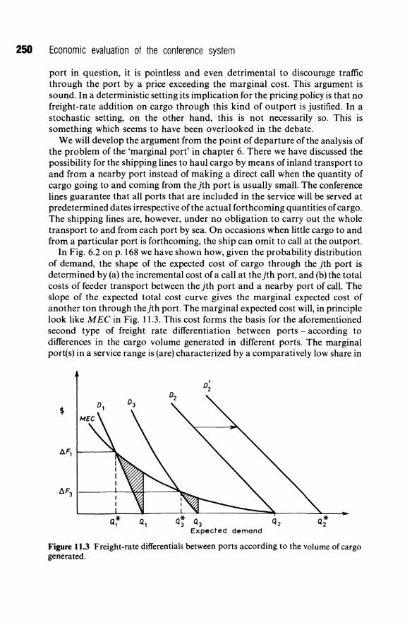
250 Economic evaluation of the conference system
port in question, it is pointless and even detrimental to discourage traffic through the port by a price exceeding the marginal cost. This argument is sound. In a deterministic setting its implication for the pricing policy is that no freight-rate addition on cargo through this kind of outport is justified. In a stochastic setting, on the other hand, this is not necessarily so. This is something which seems to have been overlooked in the debate.
We will develop the argument from the point of departure of the analysis of the problem of the 'marginal port' in chapter 6. There we have discussed the possibility for the shipping lines to haul cargo by means of inland transport to and from a nearby port instead of making a direct call when the quantity of cargo going to and coming from the jth port is usually small. The conference lines guarantee that all ports that are included in the service will be served at predetermined dates irrespective ofthe actual forthcoming quantities of cargo. The shipping lines are, however, under no obligation to carry out the whole transport to and from each port by sea. On occasions when little cargo to and from a particular port is forthcoming, the ship can omit to call at the outport.
In Fig. 6.2 on p. 168 we have shown how, given the probability distribution of demand, the shape of the expected cost of cargo through the jth port is determined by (a) the incremental cost of a call at the jth port, and (b) the total costs of feeder transport between the jth port and a nearby port of call. The slope of the expected total cost curve gives the marginal expected cost of another ton through thejth port. The marginal expected cost will, in principle look like M EC in Fig. 11.3. This cost forms the basis for the aforementioned second type of freight rate differentiation between ports - according to differences in the cargo volume generated in different ports. The marginal port(s) in a service range is (are) characterized by a comparatively low share in
A~ I------~--~~----~~
a' 2
Q, * Q3 Q3 Q2
Expected demand
Q* 2
Figure 11.3 Freight-rate differentials between ports according to the volume of cargo generated.

The freight rate and marginal cost structures 251
the total cargo volume of the trade. In Fig. 11.3 we show how differences in the shares of the trade should be reflected in the freight-rate structure, on the neutral assumption that all ports in the service range concerned are equal with regard to capacity and costs. Suppose that there are three ports in the range: one base port and one outport on either side. The marginal expected cost curve is the same for all ports, but each port has an individual demand curve. The base port generates the greatest demand. The intersection of the base-port demand curve and the marginal expected cost curve occurs at a level very close to zero.
In a situation without freight-rate differentiation between the ports the base port cargo volume is Q2 and the outport cargo volumes are Ql and Q3' When proper freight-rate differentials are introduced, the outport volumes decrease to Q! and Q!. The introduction of the freight-rate differentials I1F 1 and I1F 3 causes a shift to the right of the demand curve of the base port. (No shifts ofthe outport demand curves occur, because F 2 = 0.) The base-port cargo volume will increase to Q2' The sums of Ql + Q2 + Q3 and Q! + Q! + Q! may well be the same. What has happened is in the first place a redistribution of the cargo flows toward a concentration to the base port. It is also seen that the smaller the demand for a particular port is (the more to the left the demand curve is situated) the higher the freight rate differential will be.
lt is possible that a 'very marginal' port will be entirely excluded from the services after the introduction of this type of freight-rate differentiation. This can, however, not be established on the basis of the short-run cost picture of Fig. 11.3. Given the new sets of expected demands for different ports, the entire routing and scheduling should be reconsidered from scratch.
On the condition that the same ports will be served 'before and after', the efficiency gain from introducing outport freight-rate differentials can, in principle, be measured for each outport by the area between the marginal expected cost curve and the demand curve in the trade volume interval corresponding to the volumes generated with and without a proper freight-rate differential. In Fig. 11.3 the relevant areas are shaded. The gain in efficiency takes the form of a reduction in the number of calls at each outport. To obtain the net gain the consequent increase in land feeder-transport costs has to be subtracted from the savings for the shipowners.
11.4.4 Effects on optimal ship size of introducing a fat-Ieg/mea~e-Ieg freight rate differential
The failure of present freight rates to reflect trade imbalances may at first sight not seem very harmful from an allocative point of view. There is no reason to suppose anything but a very low freight-rate cross elasticity of the demands for shipping space in opposite directions. The rise of fat-leg levels of freight rates and the lowering of meagre-leg levels of freight rates will in general not influence the pattern of trade flows very much.
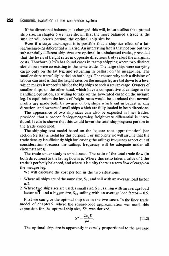
252 Economic evaluation of the conference system
If the directional balance, }1, is changed this will, in turn, affect the optimal ship size. In chapter 5 we have shown that the more balanced a trade is, the smaller will, ceteris paribus, the optimal ship size be.
Even if }1 stays unchanged, it is possible that a ship-size effect of a fatleg/meagre-leg differential will arise. An interesting fact is that not one but two substantially different ship sizes are optimal in unbalanced trades, provided that the levels of freight rates in opposite directions truly reflect the marginal costs. Thorburn (1960) has found cases in tramp shipping where two distinct size classes were co-existing in the same trade. The large ships were carrying cargo only on the fat leg, and returning in ballast on the meagre leg. The smaller ships were fully loaded on both legs. The reason why such a division of labour can arise is that the freight rates on the meagre leg are bid down to a level which makes it unprofitable for the big ships to seek a return cargo. Owners of smaller ships, on the other hand, which have a comparative advantage in the handling operation, are willing to take on the low-rated cargo on the meagre leg. In equilibrium the levels of freight rates would be so related that normal profits are made both by owners of big ships which sail in ballast in one direction, and owners of small ships which are fully loaded in both directions.
The appearance of two ship sizes can also be expected in liner trades, provided that a proper fat-Ieg/meagre-Ieg freight-rate differential is introduced. It can be shown that this would lower the total shipping cost per ton in the trade concerned.
The shipping cost model based on the 'square root approximation' (see section 6.2.1(a)) is I.seful for this purpose. For simplicity we will assume that the trade density is sufficiently high for leaving the sailings frequency aspect out of consideration (because the sailings frequency will be adequate under all circumstances).
The trade under study is unbalanced. The ratio of the total trade flow (in both directions) to the fat leg flow is }1. Where this ratio takes a value of 2 the trade is perfectly balanced, and where it is unity there is a zero flow of cargo on the meagre leg.
We will calculate the cost per ton in the two situations:
Where all ships are of the same size, S l' and sail with an average load factor }1/2.
2 Where t~o ship sizes are used; a small size, S 21' sailing with an average load factor = i, and a bigger size, S 22 sailing with an average load factor = 0.5.
First we can give the optimal ship size in the two cases. In the liner trade model of chapter 9, where the square-root approximation was used, this expression for the optimal ship size, S*, was derived:
S* = 2a 2D. }1a 1
(11.2)
The optimal ship size is apparently inversely proportional to the average

The freight rate and marginal cost structures 253
load factor f-l/2. We thus have:
( 11.3)
and
The three sizes are as seen ranked in this order:
S2l < Sl < S22·
The corresponding costs per ton are directly obtained from equation (9.19) by inserting the respective average load factors in the right-hand term, and ignoring the left-hand term (which stands for feeder transport and storage costs) of the equation.
(11.4)
and
The three costs are as seen ranked in this order:
C 2l < C l < C 22 ·
The relevant comparison is between C l and the weighed average of C2l and C22 , which is designated C2 . The relevant weights are 2(f-l- 1) and 2 - f-l. (The ratio of the total cargo carried by the smaller ships to the total cargo carried by the bigger ships is equal to 2(f-l- 1)/(2 - f-l)).
C2 __ 2(f-l- I)C2l + (2 - f-l)C22
f-l
4(f-l- l)a l a2D + 2(2 - f-l)2a l a2 D
f-l
(11.5)
After some rearrangements C 2 can be written as a product of C 1 and a factor which is solely determined by f-l.
C -C [J(2)+f-l][J(2)-I] 2- 1 Jf-l . (11.6)
The question is, whether the right-hand factor is smaller or greater than unity? For both extreme values of f-l, 1 and 2, respectively, the factor is equal to unity as expected. Both in a perfectly balanced trade, and in a trade where zero cargo moves on the meagre leg, a single ship size is optimal for obvious reasons.
For all in-between values of f-l the right-hand factor takes values which are less than unity. It can be concluded that in unbalanced trades the total costs per ton, C 2, obtained by using two ship sizes is lower than the costs per ton, C 1,
obtained by using a single ship size.
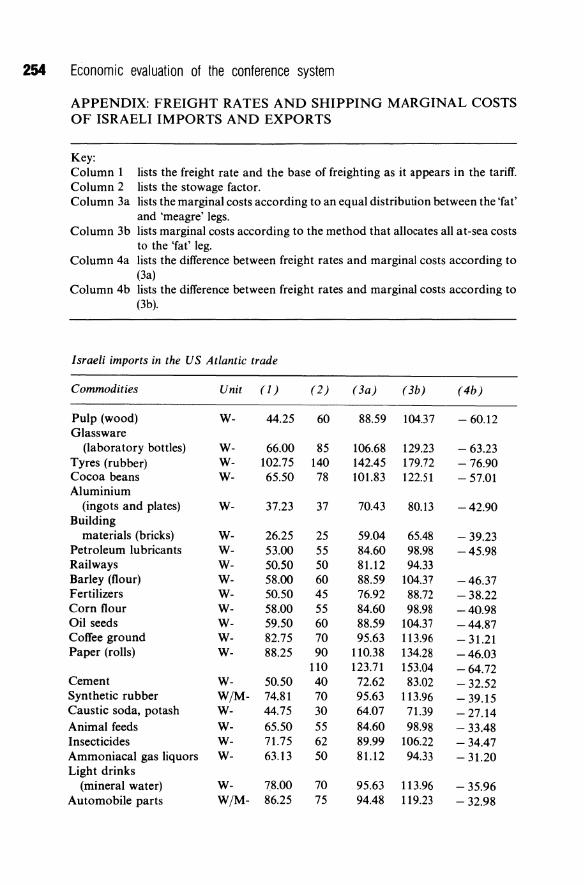
254 Economic evaluation of the conference system
APPENDIX: FREIGHT RATES AND SHIPPING MARGINAL COSTS OF ISRAELI IMPORTS AND EXPORTS
Key: Column 1 lists the freight rate and the base of freighting as it appears in the tariff. Column 2 lists the stowage factor. Column 3a lists the marginal costs according to an equal distribution between the 'fat'
and 'meagre' legs. Column 3b lists marginal costs according to the method that allocates all at-sea costs
to the 'fat' leg. Column 4a lists the difference between freight rates and marginal costs according to
(3a) Column 4b lists the difference between freight rates and marginal costs according to
(3b).
Israeli imports in the US Atlantic trade
Commodities Unit (1) (2) (3a) (3b) (4b)
Pulp (wood) w- 44.25 60 88.59 104.37 - 60.12 Glassware
(laboratory bottles) w- 66.00 85 106.68 129.23 - 63.23 Tyres (rubber) w- 102.75 140 142.45 179.72 -76.90 Cocoa beans w- 65.50 78 101.83 122.51 - 57.01 Aluminium
(ingots and plates) w- 37.23 37 70.43 80.13 -42.90 Building
materials (bricks) w- 26.25 25 59.04 65.48 - 39.23 Petroleum lubricants w- 53.00 55 84.60 98.98 -45.98 Railways W- 50.50 50 81.12 94.33 Barley (flour) W- 58.00 60 88.59 104.37 -46.37 Fertilizers W- 50.50 45 76.92 88.72 - 38.22 Corn flour W- 58.00 55 84.60 98.98 -40.98 Oil seeds W- 59.50 60 88.59 104.37 -44.87 Coffee ground W- 82.75 70 95.63 113.96 - 31.21 Paper (rolls) W- 88.25 90 110.38 134.28 -46.03
110 123.71 153.04 -64.72 Cement W- 50.50 40 72.62 83.02 - 32.52 Synthetic rubber WjM- 74.81 70 95.63 113.96 - 39.15 Caustic soda, potash w- 44.75 30 64.07 71.39 - 27.14 Animal feeds w- 65.50 55 84.60 98.98 - 33.48 Insecticides W- 71.75 62 89.99 106.22 - 34.47 Ammoniacal gas liquors W- 63.13 50 81.12 94.33 - 31.20 Light drinks
(mineral water) W- 78.00 70 95.63 113.96 - 35.96 Automobile parts WjM- 86.25 75 94.48 119.23 - 32.98

(Contd.)
Commodities Unit (1) (2) (3a) (3b) (4b)
Nuts W- 95.25 70 110.32 134.28 - 39.03 Starches w- 97.75 80 103.16 124.30 - 26.55 Paperboard w- 81.75 70 95.62 113.96 - 32.21 Asbestos sheets w- 68.13 50 81.12 94.33 - 25.90 Honey W- 67.00 48 79.19 91.70 -24.70 Pitch petroleum W- 66.00 45 76.92 88.72 - 22.72 Copper wire WjM- 57.31 35 68.11 77.11 -19.80 Sugar W 69.00 47 78.47 90.74 - 21.70 Raw wool W- 116.50 100 123.29 143.25 - 26.50
200 182.31 232.19 - 115.69 Pigments and paints WjM- 49.74 23 56.39 62.13 - 12.39 Fruit and vegetable
juices W- 78.00 55 84.60 98.98 - 20.98 Milk powder W- 89.25 68 94.42 112.28 -29.03 Steel (tubes, bars) W- 50.50 20 53.96 58.73 -8.23
40 72.62 83.02 - 32.52 Wood blocks W- 73.00 45 76.92 88.72 - 15.72 Rails (steel) W- 44.00 15 47.63 51.28 -7.28 Copper mate and copper
waste W- 49.50 18 51.76 56.33 -6.83 Hydrocarbons (gas) W- 65.25 33 66.46 75.00 -9.75 Vegetables, fruits
(fresh) W- 68.00 50 31.12 94.33 - 16.33 90 110.32 134.28 - 56.88
Fruits (dried) W- 78.00 50 81.18 74.33 - 16.33 Metal cuttings WjM- 72.56 45 76.92 88.72 - 16.16 Nickel ingots W- 61.50 12 44.26 47.21 14.29 Printed matter (books) WjM- 105.88 55 84.60 98.98 6.90 Fish, fish products W- 132.00 50 81.12 94.33 -2.28
90 110.32 134.28 37.57 Agricultural (p) W 172.50 125 148.92 189.Q1 - 16.51
machinery (v) 222.18 33.17 Jute fibres W- 123.19 73 98.15 117.42 5.77 Sporting ammunition WjM- 114.61 53 83.24 97.14 17.47 Military equipment WjM- 81.25 (50) 81.12 94.33 -13.08
138.13 (85) 106.68 129.23 8.90 Meat extract, juices W- 116.75 55 84.60 98.98 17.77 Chocolate WjM- 126.25 65 92.55 109.73 16.52 Stainless steel W- 78.00 10-12 43.04 45.76 32.24 Photographic mats WjM- 127.50 60 88.59 104.37 23.13 Soups WjM- 129.75 60 88.59 104.37 25.38 Yarn (synthetic) W- 173.25 120 76.11 161.77 11.48 Leather goods Ft- 164.00 105 120.30 148.82 15.18 Animal oil, fat W- 118.50 39 71.90 82.06 36.44
(Contd.)
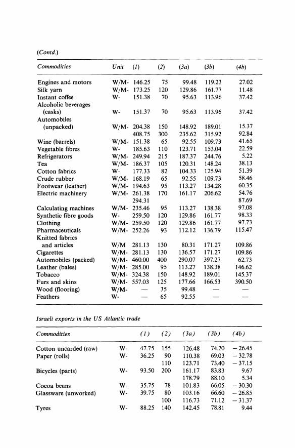
(Contd.)
Commodities Unit (1) (2) (3a) (3b) (4b)
Engines and motors W/M- 146.25 75 99.48 119.23 27.02 Silk yarn W/M- 173.25 120 129.86 161.77 11.48 Instant coffee W- 151.38 70 95.63 113.96 37.42 Alcoholic beverages
(casks) W- 151.37 70 95.63 113.96 37.42 Automobiles
(unpacked) W/M- 204.38 150 148.92 189.01 15.37 408.75 300 235.62 315.92 92.84
Wine (barrels) W/M- 151.38 65 92.55 109.73 41.65 Vegetable fibres W- 185.63 110 123.71 153.04 22.59 Refrigerators W/M- 249.94 215 187.37 244.76 5.22 Tea W/M- 186.37 105 120.31 148.24 38.13 Cotton fabrics W- 177.33 82 104.33 125.94 51.39 Crude rubber W/M- 168.19 65 92.55 109.73 58.46 Footwear (leather) W/M- 194.63 95 113.27 134.28 60.35 Electric machinery W/M- 261.38 170 161.17 206.62 54.76
294.31 87.69 Calculating machines W/M- 235.46 95 113.27 138.38 97.08 Synthetic fibre goods W- 259.50 120 129.86 161.77 98.33 Clothing W/M- 259.50 120 129.86 161.77 97.73 Pharmaceuticals W/M- 252.26 93 112.12 136.79 115.47 Knitted fabrics
and articles W/M 281.13 130 80.31 171.27 109.86 Cigarettes W/M- 281.13 130 136.57 171.27 109.86 Automobiles (packed) W/M- 460.00 400 290.07 397.27 62.73 Leather (bales) W/M- 285.00 95 113.27 138.38 146.62 Tobacco W/M- 324.38 150 148.92 189.01 145.37 Furs and skins W/M- 557.03 125 177.66 166.53 390.50 Wood (flooring) W/M- 35 99.48 Feathers W- 65 92.55
Israeli exports in the US Atlantic trade
Commodities (1) (2) (3a) (3b) (4b)
Cotton uncarded (raw) W- 47.75 155 126.48 74.20 - 26.45 Paper (rolls) W- 36.25 90 110.38 69.03 - 32.78
110 123.71 73.40 - 37.15 Bicycles (parts) W- 93.50 200 161.17 83.83 9.67
178.79 88.10 5.34 Cocoa beans W- 35.75 78 101.83 66.05 - 30.30 Glassware (un worked) W- 39.75 80 103.16 66.60 - 26.85
100 116.73 71.12 - 31.37 Tyres W- 88.25 140 142.45 78.81 9.44

(Contd.)
Commodities (1) (2) (3a) (3b) (4b)
Light drinks (mineral water) w- 45.25 70 95.63 63.77 - 18.52
Chemicals (harmless) w- 46.75 70 95.63 63.77 -17.02 Glues w- 48.50 70 95.63 63.77 -15.27 Pharmaceuticals
(medicines) w- 65.75 93 112.12 69.67 -3.92 Glassware (bottles) W- 61.25 85 106.38 67.75 -6.50 Milk powder w- 49.50 68 94.42 63.36 - 13.86 Glass (plates, sheets) w- 33.00 43 74.77 55.15 - 12.15 Oil seeds w- 48.00 60 28.59 61.18 - 13.08 Asbestos sheets w- 41.00 50 81.12 57.96 -16.96 Fertilizers w- 41.75 45 76.92 56.11 - 14.36 Wood blocks W- 13.00 45 76.92 56.11 - 13.11 Tea W/M- 86.63 105 120.31 72.36 14.27 Honey w- 47.25 48 79.90 57.30 -10.05 Garden and field seeds w- 50.00 50 81.12 57.96 -7.96
100 116.73 71.12 - 21.12 Metal scrap w- 50.00 30 64.07 50.00 0
81.12 57.96 -7.96 Printer matter (books) W/M- 54.66 55 84.60 59.47 -4.81 Steel (tubes, bars) w- 43.25 20 53.96 54.19 - 1.16
40 72.62 44.41 -10.94 Preserves w- 55.25 55 84.60 59.47 -4.22 Chocolate w- 63.25 65 92.55 62.67 0.58 Ammoniacal liquors w- 81.25 50 81.12 69.03 12.22 Nuts w- 53.75 90 110.32 57.96 -4.23 Alcoholic beverages
(casks) w- 72.25 70 95.63 63.77 8.48 Linoleum, floor covers w- 75.00 70 95.62 56.11 18.89 Sporting ammunition w- 63.25 53 83.24 58.89 4.36 Wine (barrels) w- 72.75 65 92.55 62.67 10.08 Automobile parts W/M- 82.50 75 99.48 65.28 17.22 Fruit and vegetable
juices w- 88.75 55 84.60 59.47 8.32 Starches w- 88.75 80 103.10 66.60 22.15 Building materials (bricks) W- 44.75 25 59.04 47.37 -2.62 Pigments, paints W/M- 42.26 23 56.39 45.92 -3.66 Soups w- 76.50 60 88.59 61.08 15.42 Jams, jellies w- 80.50 45 91.50 56.11 24.39 Tractor parts W/M- 88.59 75 99.48 65.28 23.31 Raw wool w- 63.00 100 123.29 71.12 - 8.12
200 182.31 88.16 - 25.16 Aluminium (ingots
and plates) W- 63.00 37 70.43 53.21 9.79 Fruits (dried) w- 77.00 50 81.12 57.96 19.04
(Contd.)

(Contd.)
Commodities (1) (2) (3a) (3b) (4b)
Veneer and plywood Ft- 143.06 75 120.30 65.28 77.78 Leather goods Ft- 143.06 105 120.30 72.36 70.70 Polyethylene sheets W/M- 121.19 70 95.62 63.77 57.42 Nickel ingots W- 76.00 12 44.26 38.60 37.40 Meat extract, juices W- 131.50 55 84.60 59.47 72.03 Clothing W/M- 189.75 120 129.86 75.24 114.51 Fish, fish products W- 144.00 50 81.12 57.96 86.04
90 110.32 69.03 74.97 Refrigerators W/M- 255.31 215 187.37 90.11 165.20 Plastic articles W- 161.75 65 92.55 62.67 99.03 Footwear (leather) W/M- 194.25 95 113.27 69.03 125.22 Agricultural machinery (p)W- 200.63 125 148.92 80.59 120.04
(v) 233.44 152.85
Instant coffee W- 212.50 70 95.63 63.77 148.73 Synthetic fibre goods W- 50.25 120 129.86 75.24 175.01 Knitted fabrics articles W/M- 221.81 130 80.31 72.24 149.57
Automobiles W/M- 191.25 150 148.92 80.59 110.66 (unpacked) 382.50 300 235.62 100.14 282.36
Automobiles (packed) W/M- 445.00 400 290.07 109.81 335.19 Electric Mechinery W/M- 333.63 170 161.17 83.83 249.80 Feathers W- 354.25 65.90 92.55 62.67 285.22
69.03 291.58
Israeli exports in the Mediterranean trade by conventional liners
Commodities (1) (2) (3b) (4b)
Bricks W- 12.01 25 31.28 -14.20 Paper W- 17.02 96 27.33 - 10.31 Tyres W/M- 36.14 85 26.19 -9.95 Vipla W- 20.57 110 29.70 - 9.45 Urea W- 17.02 75 24.68 -7.66 Seeds W- 17.02 55-70 21.49 -6.99
24.01 -4.47 Carbon black W- 25.91 115 30.24 -5.03 Copper plates W/M- 8.39 16 13.20 -4.31 Greasy wool W- 27.39 122 31.39 -3.70 Metal ingots W- 16.49 35 14.43 -3.02
15.49 40 18.51 1.06 Light drinks
(soda water) W- 21.08 70 24.01 -2.93 Cement W- 17.02 40 18.84 -1.82 Coffee (ground) bags W- 22.35 70 24.01 -1.66
tins W/M- 42.90 18.39 Beans, peas W- 20.07 56 21.11 -1.07
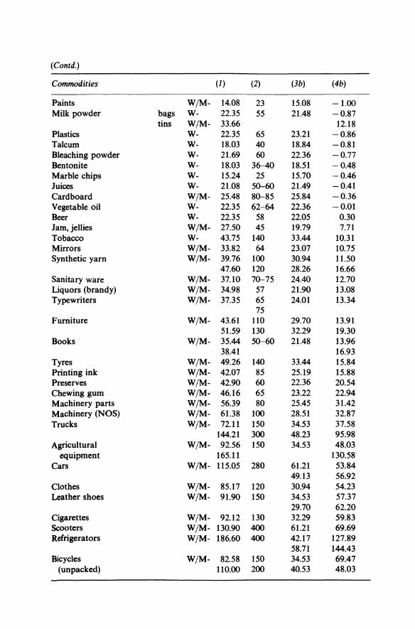
(Contd.)
Commodities (1) (2) (3b) (4b)
Paints W/M- 14.08 23 15.08 -1.00 Milk powder bags W- 22.35 55 21.48 -0.87
tins W/M- 33.66 12.18 Plastics W- 22.35 65 23.21 -0.86 Talcum W- 18.03 40 18.84 -0.81 Bleaching powder W- 21.69 60 22.36 -0.77 Bentonite W- 18.03 36-40 18.51 -0.48 Marble chips W- 15.24 25 15.70 -0.46 Juices W- 21.08 50-60 21.49 -0.41 Cardboard W/M- 25.48 80-85 25.84 -0.36 Vegetable oil W- 22.35 62-64 22.36 -0.01 Beer W- 22.35 58 22.05 0.30 Jam, jellies W/M- 27.50 45 19.79 7.71 Tobacco W- 43.75 140 33.44 10.31 Mirrors W/M- 33.82 64 23.07 10.75 Synthetic yarn W/M- 39.76 100 30.94 11.50
47.60 120 28.26 16.66 Sanitary ware W/M- 37.10 70-75 24.40 12.70 Liquors (brandy) W/M- 34.98 57 21.90 13.08 Typewriters W/M- 37.35 65 24.01 13.34
75 Furniture W/M- 43.61 110 29.70 13.91
51.59 130 32.29 19.30 Books W/M- 35.44 50-60 21.48 13.96
38.41 16.93 Tyres W/M- 49.26 140 33.44 15.84 Printing ink W/M- 42.07 85 25.19 15.88 Preserves W/M- 42.90 60 22.36 20.54 Chewing gum W/M- 46.16 65 23.22 22.94 Machinery parts W/M- 56.39 80 25.45 31.42 Machinery (NOS) W/M- 61.38 100 28.51 32.87 Trucks W/M- 72.11 150 34.53 37.58
144.21 300 48.23 95.98 Agricultural W/M- 92.56 150 34.53 48.03
equipment 165.11 130.58 Cars W/M- 115.05 280 61.21 53.84
49.13 56.92 Clothes W/M- 85.17 120 30.94 54.23 Leather shoes W/M- 91.90 150 34.53 57.37
29.70 62.20 Cigarettes W/M- 92.12 130 32.29 59.83 Scooters W/M- 130.90 400 61.21 69.69 Refrigerators W/M- 186.60 400 42.17 127.89
58.71 144.43 Bicycles W/M- 82.58 150 34.53 69.47
(unpacked) 110.00 200 40.53 48.03
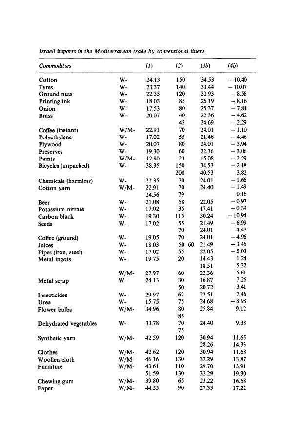
Israeli imports in the Mediterranean trade by conventional liners
Commodities (1) (2) (3b) (4b)
Cotton W- 24.13 150 34.53 -10.40 Tyres W- 23.37 140 33.44 -10.07 Ground nuts W- 22.35 120 30.93 -8.58 Printing ink W- 18.03 85 26.19 - 8.16 Onion W- 17.53 80 25.37 -7.84 Brass W- 20.07 40 22.36 -4.62
45 24.69 -2.29 Coffee (instant) W/M- 22.91 70 24.01 -1.10 Polyethylene W- 17.02 55 21.48 -4.46 Plywood W- 20.07 80 24.01 -3.94 Preserves W- 19.30 60 22.36 -3.06 Paints W/M- 12.80 23 15.08 -2.29 Bicycles (unpacked) W- 38.35 150 34.53 - 2.18
200 40.53 3.82 Chemicals (harmless) W- 22.35 70 24.01 -1.66
Cotton yam W/M- 22.91 70 24.40 -1.49 24.56 79 0.16
Beer W- 21.08 58 22.05 -0.97 Potassium nitrate W- 17.02 35 17.41 -0.39 Carbon black W- 19.30 115 30.24 -10.94 Seeds W- 17.02 55 21.49 -6.99
70 24.01 -4.47 Coffee (ground) W- 19.05 70 24.01 -4.96 Juices W- 18.03 50-60 21.49 -3.46 Pipes (iron, steel) W- 17.02 55 22.05 -5.03 Metal ingots W- 19.75 20 14.43 1.24
18.51 5.32 W/M- 27.97 60 22.36 5.61
Metal scrap W- 24.13 30 16.87 7.26 50 20.72 3.41
Insecticides W- 29.97 62 22.51 7.46 Urea W- 15.75 75 24.68 -8.98
Flower bulbs W/M- 34.96 80 25.84 9.12 85
Dehydrated vegetables W- 33.78 70 24.40 9.38 75
Synthetic yam W/M- 42.59 120 30.94 11.65 28.26 14.33
Clothes W/M- 42.62 120 30.94 11.68 Woollen cloth W/M- 46.16 130 32.29 13.87 Furniture W/M- 43.61 110 29.70 13.91
51.59 130 32.29 19.30 Chewing gum W/M- 39.80 65 23.22 16.58 Paper W/M- 44.55 90 27.33 17.22
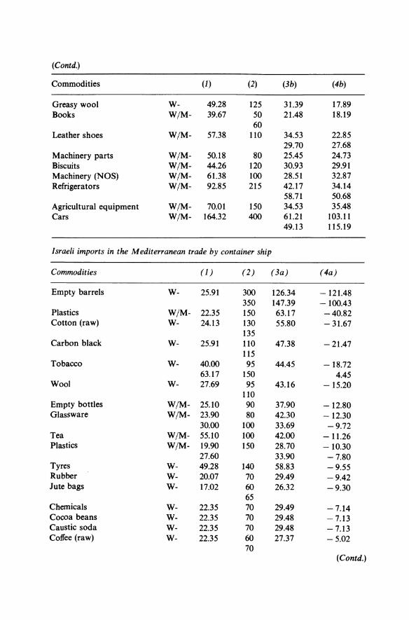
(Contd.)
Commodities (1) (2) (3b) (4b)
Greasy wool W- 49.28 125 31.39 17.89 Books W/M- 39.67 50 21.48 18.19
60 Leather shoes W/M- 57.38 110 34.53 22.85
29.70 27.68 Machinery parts W/M- 50.18 80 25.45 24.73 Biscuits W/M- 44.26 120 30.93 29.91 Machinery (NOS) W/M- 61.38 100 28.51 32.87 Refrigerators W/M- 92.85 215 42.17 34.14
58.71 50.68 Agricultural equipment W/M- 70.01 150 34.53 35.48 Cars W/M- 164.32 400 61.21 103.11
49.13 115.19
Israeli imports in the Mediterranean trade by container ship
Commodities (1) (2) (3a) (4a)
Empty barrels W- 25.91 300 126.34 - 121.48 350 147.39 -100.43
Plastics W/M- 22.35 150 63.17 -40.82 Cotton (raw) W- 24.13 130 55.80 - 31.67
135 Carbon black W- 25.91 110 47.38 - 21.47
115 Tobacco W- 40.00 95 44.45 -18.72
63.17 150 4.45 Wool W- 27.69 95 43.16 -15.20
110 Empty bottles W/M- 25.10 90 37.90 -12.80 Glassware W/M- 23.90 80 42.30 -12.30
30.00 100 33.69 -9.72 Tea W/M- 55.10 100 42.00 - 11.26 Plastics W/M- 19.90 150 28.70 -10.30
27.60 33.90 -7.80 Tyres W- 49.28 140 58.83 -9.55 Rubber W- 20.07 70 29.49 -9.42 Jute bags W- 17.02 60 26.32 -9.30
65 Chemicals W- 22.35 70 29.49 -7.14 Cocoa beans W- 22.35 70 29.48 -7.13 Caustic soda W- 22.35 70 29.48 -7.13 Coffee (raw) W- 22.35 60 27.37 -5.02
70 (Contd.)
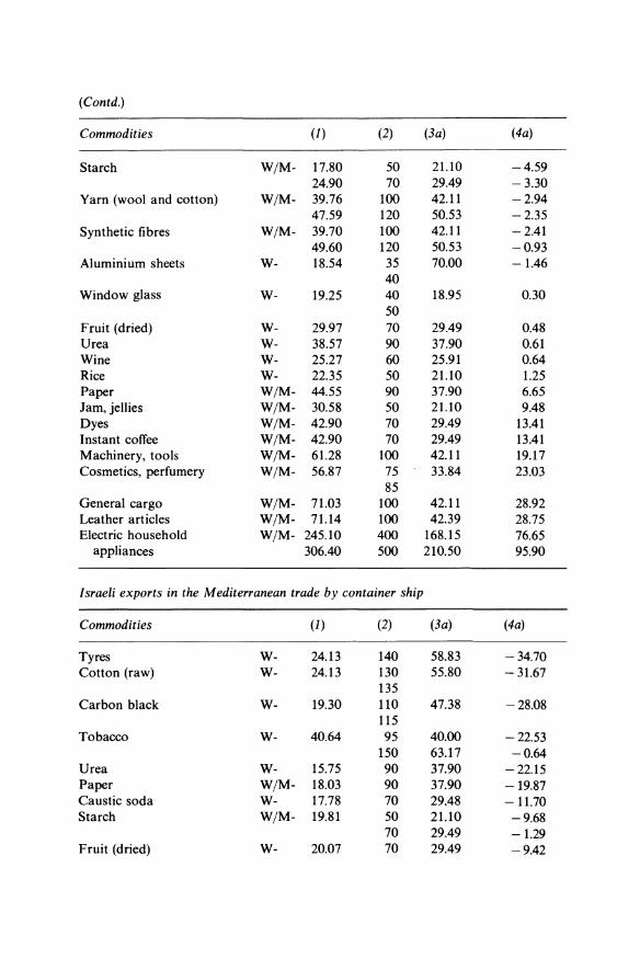
(Contd.)
Commodities (1) (2) (3a) (4a)
Starch W/M- 17.80 50 21.10 -4.59 24.90 70 29.49 -3.30
Yarn (wool and cotton) W/M- 39.76 100 42.11 -2.94 47.59 120 50.53 -2.35
Synthetic fibres W/M- 39.70 100 42.11 - 2.41 49.60 120 50.53 -0.93
Aluminium sheets W- 18.54 35 70.00 -1.46 40
Window glass W- 19.25 40 18.95 0.30 50
Fruit (dried) W- 29.97 70 29.49 0.48 Urea W- 38.57 90 37.90 0.61 Wine W- 25.27 60 25.91 0.64 Rice W- 22.35 50 21.10 1.25 Paper W/M- 44.55 90 37.90 6.65 Jam, jellies W/M- 30.58 50 21.10 9.48 Dyes W/M- 42.90 70 29.49 13.41 Instant coffee W/M- 42.90 70 29.49 13.41 Machinery, tools W/M- 61.28 100 42.11 19.17 Cosmetics, perfumery W/M- 56.87 75 33.84 23.03
85 General cargo W/M- 71.03 100 42.11 28.92 Leather articles W/M- 71.14 100 42.39 28.75 Electric household W/M- 245.10 400 168.15 76.65
appliances 306.40 500 210.50 95.90
Israeli exports in the Mediterranean trade by container ship
Commodities (1) (2) (3a) (4a)
Tyres W- 24.13 140 58.83 - 34.70 Cotton (raw) W- 24.13 130 55.80 - 31.67
135 Carbon black W- 19.30 110 47.38 -28.08
115 Tobacco W- 40.64 95 40.00 -22.53
150 63.17 -0.64 Urea W- 15.75 90 37.90 - 22.15 Paper W/M- 18.03 90 37.90 -19.87 Caustic soda W- 17.78 70 29.48 - 11.70 Starch W/M- 19.81 50 21.10 -9.68
70 29.49 -1.29 Fruit (dried) W- 20.07 70 29.49 -9.42
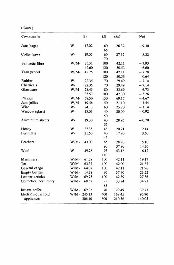
(Contd.)
Commodities (1) (2) (3a) (4a)
Jute (bags) W- 17.02 60 26.32 -9.30 65
Coffee (raw) W- 19.05 60 27.37 - 8.32 70
Synthetic fibre W/M- 35.51 100 42.11 -7.93 42.60 120 50.53 -6.60
Yarn (wool) W/M- 42.75 100 42.11 -7.78 120 50.53 -0.64
Rubber W- 22.35 70 29.49 -7.14 Chemicals W- 22.35 70 29.49 -7.14 Glassware W/M- 28.43 80 33.69 -6.73
35.57 100 42.30 -5.26 Plastics W/M- 58.50 150 69.17 -4.67 Jam, jellies W/M- 19.56 50 21.10 -1.54 Wine W- 24.13 60 25.20 - 1.14 Window (glass) W- 18.03 40 20.00 -0.92
50 Aluminium sheets W- 19.30 40 28.95 -0.70
35 Honey W- 22.35 48 20.21 2.14 Fertilizers W- 21.50 40 17.90 3.60
45 Feathers W/M- 43.00 65 28.70 5.10
90 37.90 14.30 Wool W- 49.28 95 43.16 6.12
110 Machinery W/M- 61.28 100 42.11 19.17 Tea W/M- 63.37 100 42.00 21.37 General cargo W/M- 64.07 100 42.11 21.96 Empty bottles W/M- 14.38 90 37.90 23.52 Leather articles W/M- 69.75 100 42.39 27.36 Cosmetics, perfumery W/M- 68.57 75 33.84 34.73
85 Instant coffee W/M- 69.22 70 29.49 39.73 Electric household W/M- 245.13 400 168.45 95.90
appliances 306.40 500 210.56 140.05

12 Potential cartel profits become social costs
The divergences between existing freight-rate structures and the marginal cost structure discussed in the previous chapter are bad. Even worse, we think is another source of inefficiency, namely: the price-rigging power itself of linershipping conferences easily causes both excess capacity and excessive service competition between conference members. It has puzzled many observers that in the thoroughly cartelized liner-shipping industry, supernormal profits are generally absent. Some commentators have suggested that liner-shipping companies do not want to maximize profits. A more plausible explanation, in our view, is that the potential monopoly profits are turned into costs - costs of inputs into the fight for the expected reward. Compare Posner (1975), who summarizes the general phenomenon thus: 'Competition to obtain a monopoly results in the transformation of expected monopoly profits into social costs.'
The transformation of potential monopoly profits into social costs can take somewhat different forms. A basic common feature is that, in the first place, rigged freight rates will induce individual lines to compete by putting in more ships on the route, in order to increase their share in the trade. Given a level of freight rates well above the level of marginal costs, it is profitable (from a private point of view) for an individual line to increase its sailings. The trouble is, of course, that every shipping line tries the same thing, with the end result of high costs and low profits for everybody. The exertion of the price-fixing power of liner conferences, tends to raise the level of costs to practically any level of freight rates that is initially established.
In the second stage, given low load factors and the absence of super-normal profits, two things can happen: first individual lines are now willing to carry relatively low-rated minor bulk cargo for filling up space, and secondly each individual shipping line will try to overbid its competitors for high-rated cargo in respect of various qualities of service, with the end result of a too high quality of service from a welfare economic point of view, and a further increase in costs.
12.1 EMPIRICAL EVIDENCE OF LOW LOAD FACTORS IN LINER SHIPPING
In spite of the fact that liners are filling up empty space by tramp cargo as far as possible, rather low load factors can be observed. In the 1980s the main explanation for this is the over-supply of container ships ordered in the boom period of the 1970s. But even in the year of 1979, for which we have very
Cartel profits and social costs 263
carefully compiled statistics, it seems that load factors were rather low, at least in trades to and from the USA.
The calculation of capacity utilization was made possible by the carefully compiled statistics of the USA trade in 1979, compiled by Captain Zvi Idelstein (Effects of Marketing Structure. Organization and Conduct on the Rate Making Process, unpublished 1981). It was done by dividing the total trade measured in cubic meters, carried between USA East and West Coasts and all foreign trade areas, by the total annual capacity offered, measured in TEUs. Cargo quantities measured comprised all liner trade to and from all foreign ports in the countries trading with the USA, to and from the following USA ports:
North Atlantic: Boston, New York, Philadelphia, Baltimore, Norfolk, Newport News.
South Atlantic: Savannah, Charleston, Jacksonville, Miami.
Pacific: Portland, Seattle, Stockton, Oakland, San Francisco, Los Angeles, Long Beach, San Diego.
Gulf: Tampa, New Orleans, Houston, Galveston.
Capacity offered was calculated on the basis of actual sizes of vessels sailing on these routes and their actual frequencies. This was done for each of the nine trading areas listed in Table 12.1. In cases where the same ships were used for trading to Canada, the available capacity offered to the USA trade was reduced accordingly. All trade examined was containerized cargo. Therefore, shipping capacity was expressed in standard container units, where a ship of 15000 dwt is equivalent to 1000 TEUs.
The capacity utilization was calculated by us for the fat leg only. It was calculated by dividing the actual volume carried per container, by the maximum volume capacity per container which was taken to be 1060 cubic feet, or 30.23 cubic metres. The resulting load factors are very low (column 4.1). The average container capacity utilization in 1979 in USA seaborne trade was equal to 0.326. Even after allowance for 50% broken stowage of commodities, load factors on all trade routes except the Far East and South East Asia remained low. The average capacity utilization in this case amounted to 0.49.
12.2 MODEL OF SUPPLY AND DEMAND EQUILIBRIUM IN A LINER TRADE
We will here present a model of how supply and demand equilibrium is brought about in a liner-shipping cartel. Rather than drawing on one of the existing approaches to cartel and oligopoly theory our model is based on a feature which is the key to understanding why liner shipping is so prone to excess capacity, and which is exclusively associated with the provision of

Tab
le 1
2.1
Cap
acit
y ut
iliz
atio
n o
f con
tain
er s
ervi
ces
in t
he U
SA t
rade
(19
79)
Uti
liza
tion
Uti
liza
tion
rat
e (i
n vo
lum
e)
Supp
ly o
f shi
ppin
g (4
) T
rade
Vol
ume
capa
city
C
ubic
(1
) (2
) m
etri
c N
o a
llow
ance
50
%
tons
per
fo
r br
oken
al
low
ance
U
S Im
port
E
xpor
t 10
00
1000
T
EU
st
owag
e fo
r br
oken
T
rade
are
a re
gion
( 1
000
c.m
. to
ns)
dwt
TE
Us
(3)
(4.1
) st
owag
e (4
.2)
Aus
tral
ia a
nd N
ew Z
eala
nd
EC
14
17
1293
16
57
110.
46
12.8
3 0.
42
0.64
W
C
451
614
979
65.2
5 9.
41
0.31
0.
47
Far
Eas
t an
d S
outh
-E
C
7701
57
92
7689
51
2.51
15
.03
0.50
0.
75
Eas
t A
sia
WC
13
024
1642
1 16
732
1115
.47
14.7
2 0.
49
0.73
Wes
t A
fric
a E
C
245
1444
27
16
118.
05
7.98
0.
26
0.40
W
C
Sou
th a
nd E
ast
Afr
ica
EC
62
8 90
4 16
29
108.
62
8.32
0.
27
0.41
W
C
29
97
6.50
4.
46
0.15
0.
22

Nor
thw
est
Eur
ope
Bal
tic
EC
98
07
1005
6 16
479
1098
.61
9.15
0.
30
0.45
U
K a
nd I
rela
nd
WC
15
04
1111
19
39
129.
29
11.6
3 0.
38
0.58
Med
iter
rani
an a
nd
EC
47
63
5577
80
10
534.
03
10.4
4 0.
34
0.52
B
lack
Sea
W
C
645
257
826
55.0
8 11
.71
0.39
0.
58
Red
Sea
and
E
C
95
3744
65
92
439.
47
8.52
0.
28
0.42
P
ersi
an G
ulf
WC
16
1 20
5 13
.68
11.7
7 0.
39
0.58
Eas
t co
ast
Sou
th A
mer
ica
EC
24
33
4803
62
42
416.
12
11.5
4 0.
38
0.57
W
C
294
222
465
37.0
0 7.
94
0.26
0.
39
Wes
t co
ast
Sou
th A
mer
ica
EC
17
95
1592
33
31
222.
09
8.08
0.
27
0.40
W
C
202
198
660
44.0
2 4.
59
0.15
0.
23
Col
umn
(1)
lists
the
tra
de v
olum
e to
(im
port
s) a
nd f
rom
(ex
port
s) t
he U
SA;
trad
e vo
lum
e is
mea
sure
d in
cub
ic m
etri
c to
ns.
Col
umn
(2)
lists
the
sup
ply
of s
hipp
ing
capa
city
on
the
trad
e ro
utes
, m
easu
red
in d
wt
and
TE
Us
(20
foot
con
tain
er e
quiv
alen
t).
Col
umn
(3)
is c
alcu
late
d by
div
idin
g th
e vo
lum
e of
tra
de (
1) b
y th
e nu
mbe
r of
TE
Us
(3)
of th
e 'fa
t' le
g of
eac
h tr
ade
rout
e.
Col
umn
(4)
the
util
izat
ion
rate
is c
alcu
late
d by
div
idin
g th
e ac
tual
vol
ume
of c
argo
car
ried
per
con
tain
er (3
) by
the
max
imum
vol
ume
that
can
be
carr
ied
-10
60
cubi
c fe
et,
or
30.2
3 cu
bic
met
ers.
E
C,
Eas
t C
oast
; W
C,
Wes
t C
oast
.
268 Economic evaluation of the conference system
scheduled transport services. The feature referred to can be summarized by the phrase 'demand follows supply'.
It should be emphasized that our rather schematic description of the mechanism that generates excess capacity does not apply to the same extent to all conferences. It applies to conferences that regulate freight rates but do not regulate supply. As far as conferences that have market sharing agreements are concerned, the future share of each line is often determined by the current capacity of its fleet on the route. Adjustments in market shares are made from time to time on the basis of the capacity offered by each line and the amount of cargo that it actually carries, so the incentive to compete by adding capacity still exists.
12.2.1 'Demand follows supply' and excess capacity
A goods manufacturer who is a price-taker can adjust to a fall in demand by reducing production capacity, without fear of losing customers. Take, for example, a manufacturer of wireless sets who is a member of a price cartel, and who produces 1000 sets per week. If demand for his products falls by 50% he can (after a while) get rid of the resulting excess capacity by making a comparable reduction in productive capacity. His previous level of capacity utilization can be maintained.
The situation is different for a shipping line. A shipowner is employing, for example, four ships on a route, but each ship is sailing half empty every voyage. At first sight, the obvious thing for the shipowner to do, in order to secure fullcapacity utilization, is to take two of his ships out of service. The trouble is, however, that business might well drop at more or less the same rate as offered capacity, and the remaining two ships would still sail half empty!
'Demand follows supply' rather than the other way round is a feature of liner-shipping services offered at a 'rigged' price. Unless rate concessions are made to the shippers originally catered for, a contracting liner has great difficulty in keeping its customers and maintaining its market share so that an appreciably higher load factor can be achieved. Shippers would have to postpone some shipments or dispatch them earlier to adjust to the sparser schedule of this shipowner, and why should they do something for nothing?
Alternatively, the shipowner in the above example may substitute four halfas-big ships for the original ships. This will raise the load factors but it will also raise the cost per unit of capacity, assuming that the original size of the ships is the optimal size for the route. Such a radical change of the fleet is, to be sure, not made in ajiffy, and, moreover, shipowners are naturally reluctant to invest in 'plant' well below best-practice size. If the competitors continue to use ships ofthe optimal size, and eventually manage to raise load factors, the shipowner stuck with the small ships will be at a serious disadvantage. It can be observed that a multi-plant goods manufacturing firm, which is reducing its total capacity, will as a matter of course, lessen the number of plants, and not the capacity per plant.

Cartel profits and social costs 269
In the following model we assume that shipping lines act in the same way, i.e. expand and contract the carrying capacity by adding and withdrawing ships, or sailings by ships of the optimal size. It seems that basically similar results would be obtained in a model where the possibility to go down in size when the load factor is unsatisfactory is allowed for, because this will also increase the cost per ton as a result of a decrease in demand.
We will assume the following setting of the model.
The flow of demand for shipping space on a particular route is uniform over time and shippers are indifferent as to which ship or shipping line takes their cargo, as long as it is the nearest in time. The first ship that offers space gets the business.
2 There is no 'flocking' of ships on the route. Equal intervals between all sailings are maintained. If a particular line wants to increase its sailing by putting an additional ship, other carriers - out of self interest - will adjust their schedule accordingly.
3 The freight rates are fixed according to the principle of charging what the traffic can bear. The average level of freight rates is thus determined by, on the one hand, the composition of cargo as to high-value and low-value commodities, and, on the other, by possible outside competition. This means that the potential monopoly profits of the conference members is exogenously given. The basic idea of the model is, however, that in equilibrium only normal profits will be earned on average. The potential profits are turned into social costs.
The following notations will be used in the model.
S = ship size; the same for all ships of all lines. F = level of freight rates, i.e. the weighted average of the freight rates of all
commodities quoted in the tariff. Q = total cargo volume on the route associated with the fixed freight rates.
We assume that the sailings frequency does not affect the total demand for shipping space.
Qi = total cargo volume carried by the ith shipping line; i = 1, ... , k. N = total number of sailings by all lines on the route. Ni = total number of sailings by the ith line.
The basic property of our model is expressed by the equality:
Qi Ni
Q N (12.1)
The market share of the ith company equals the ratio of the number of sailings of the ith company to the total number of sailings.
Equilibrium on the model route is reached when no shipping line will find it profitable to add or substract from the carrying capacity provided. This is to say, that the marginal revenue product (MRP) of a sailing of each line shall equal the incremental cost of a sailing.

270 Economic evaluation of the conference system
The MRP of a sailing of the ith company, MRPi is equal to the marginal product in terms of tons of cargo resulting from an additional sailing times the marginal revenue of a ton of cargo. The marginal product of the ith company can be expressed as the derivative ofQi with respect to N i • On the assumptions of fixed (collectively by the conference) freight rates, and of a uniform expected demand for shipping of each particular commodity, the marginal revenue equals the weighted average freight rate, F. We can thus write:
dQiMRPi=-d F.
Ni
From equation (12.1) the total carrying per year of the ith company is given:
N· Qi=Q;. (12.2)
The derivative of Qi with respect to Ni is:
dQi Q(N -Ni) dNi N 2
(12.3)
We further denote: b = the load factor, which by assumption is identical for all sailings in the trade and thus equal to the ratio of the total volume of trade, Q, to the total carrying capacity, SN. (It is interesting to note that an empirical investigation of annual average load factors of airlines supports this assumption. According to Vance (1972), 'there is little variation in the jet average load factor among airlines'.)
Si = the market share of the ith company, which by definition is equal to the ratio of Qi to Q, which in its turn equals the ratio of Ni to N.
The change in quantity carried as a result of an additional sailing of the ith company can be written in terms of band Si:
dQi - = bS(1-s.) dNi ,. (12.4)
The net cost of an additional sailing of the ith company, i.e. the total incremental cost minus the costs which are proportional to the volume of cargo handled, can, on the assumption of constant returns to scale of a firm, be expressed as the product of the ship size, S, and the shipping cost per unit of capacity (ton) of the ith company, Ci • The equilibrium condition that MRPi
should be equal to the cost of an additional sailing can consequently be written:
bS(1 - s;)F = SCi' (12.5)
This equilibrium represents a system of k equations. There are k + 1 endogenous variables: the market shares of k companies and the common load factor. By adding the identity that the sum of all market shares is unity to the
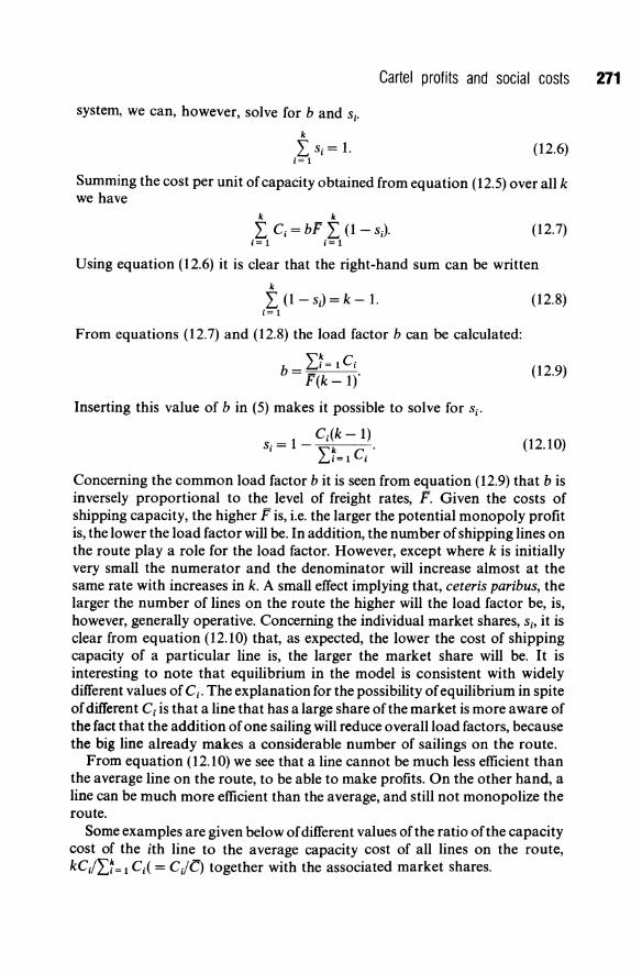
Cartel profits and social costs 271
system, we can, however, solve for band Si.
k
LSi = 1. i= 1
(12.6)
Summing the cost per unit of capacity obtained from equation (12.5) over all k we have
k k
L C i = bF L (1 - S;). (12.7) i= 1 i= 1
Using equation (12.6) it is clear that the right-hand sum can be written k
L (1 - Si) = k - 1. i= 1
From equations (12.7) and (12.8) the load factor b can be calculated:
b L7= 1 C i
= F(k-1)"
Inserting this value of b in (5) makes it possible to solve for Si.
Ci(k - 1) Si = 1-,,~ C ..
L.,1=1 I
(12.8)
(12.9)
(12.10)
Concerning the common load factor b it is seen from equation (12.9) that b is inversely proportional to the level of freight rates, F. Given the costs of shipping capacity, the higher F is, i.e. the larger the potential monopoly profit is, the lower the load factor will be. In addition, the number of shipping lines on the route playa role for the load factor. However, except where k is initially very small the numerator and the denominator will increase almost at the same rate with increases in k. A small effect implying that, ceteris paribus, the larger the number of lines on the route the higher will the load factor be, is, however, generally operative. Concerning the individual market shares, Si' it is clear from equation (12.10) that, as expected, the lower the cost of shipping capacity of a particular line is, the larger the market share will be. It is interesting to note that equilibrium in the model is consistent with widely different values of C i • The explanation for the possibility of equilibrium in spite of different Ci is that a line that has a large share ofthe market is more aware of the fact that the addition of one sailing will reduce overall load factors, because the big line already makes a considerable number of sailings on the route.
From equation (12.10) we see that a line cannot be much less efficient than the average line on the route, to be able to make profits. On the other hand, a line can be much more efficient than the average, and still not monopolize the route.
Some examples are given below of different values ofthe ratio ofthe capacity cost of the ith line to the average capacity cost of all lines on the route, kCiL~= 1 Ci ( = Ci/C) together with the associated market shares.
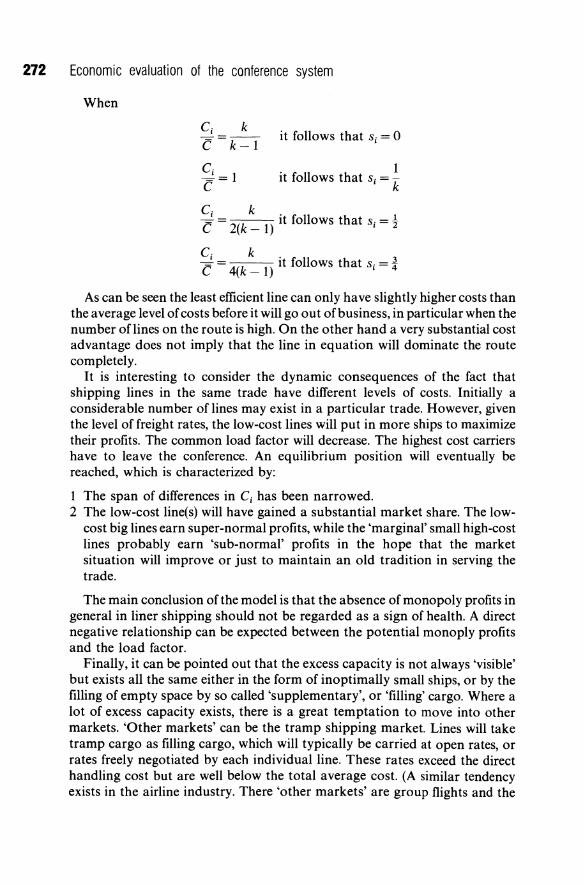
272 Economic evaluation of the conference system
When
C i k
C k-l it follows that Si = 0
C. ~-1 C- it follows that Si = ~
k . ~ 1 1 2(k _ 1) It 0 lows that Si = 2
k . 3 4(k _ 1) It follows that Si = 4
As can be seen the least efficient line can only have slightly higher costs than the average level of costs before it will go out of business, in particular when the number oflines on the route is high. On the other hand a very substantial cost advantage does not imply that the line in equation will dominate the route completely.
It is interesting to consider the dynamic consequences of the fact that shipping lines in the same trade have different levels of costs. Initially a considerable number of lines may exist in a particular trade. However, given the level of freight rates, the low-cost lines will put in more ships to maximize their profits. The common load factor will decrease. The highest cost carriers have to leave the conference. An equilibrium position will eventually be reached, which is characterized by:
1 The span of differences in C i has been narrowed. 2 The low-cost line(s) will have gained a substantial market share. The low
cost big lines earn super-normal profits, while the 'marginal' small high-cost lines probably earn 'sub-normal' profits in the hope that the market situation will improve or just to maintain an old tradition in serving the trade.
The main conclusion of the model is that the absence of monopoly profits in general in liner shipping should not be regarded as a sign of health. A direct negative relationship can be expected between the potential monoply profits and the load factor.
Finally, it can be pointed out that the excess capacity is not always 'visible' but exists all the same either in the form of inoptimally small ships, or by the filling of empty space by so called 'supplementary', or 'filling' cargo. Where a lot of excess capacity exists, there is a great temptation to move into other markets. 'Other markets' can be the tramp shipping market. Lines will take tramp cargo as filling cargo, which will typically be carried at open rates, or rates freely negotiated by each individual line. These rates exceed the direct handling cost but are well below the total average cost. (A similar tendency exists in the airline industry. There 'other markets' are group flights and the
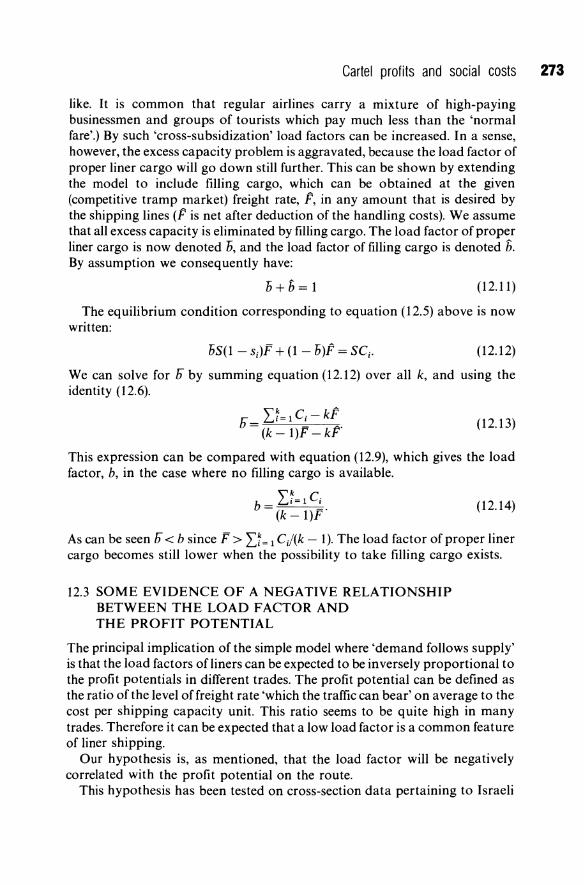
Cartel profits and social costs 273
like. It is common that regular airlines carry a mixture of high-paying businessmen and groups of tourists which pay much less than the 'normal fare'.) By such 'cross-subsidization' load factors can be increased. In a sense, however, the excess capacity problem is aggravated, because the load factor of proper liner cargo will go down still further. This can be shown by extending the model to include filling cargo, which can be obtained at the given (competitive tramp market) freight rate, F, in any amount that is desired by the shipping lines (F is net after deduction of the handling costs). We assume that all excess capacity is eliminated by filling cargo. The load factor of proper liner cargo is now denoted 0, and the load factor of filling cargo is denoted b. By assumption we consequently have:
(12.11)
The equilibrium condition corresponding to equation (12.5) above is now written:
oS(1 - sJF + (1 - o)F = SCi' (12.12)
We can solve for Ei by summing equation (12.12) over all k, and using the identity (12.6).
(12.13)
This expression can be compared with equation (12.9), which gives the load factor, b, in the case where no filling cargo is available.
b = L~=l Ci .
(k - 1)F (12.14)
As can be seen Ei < b since F > L~ = 1 C i/( k - 1). The load factor of proper liner cargo becomes still lower when the possibility to take filling cargo exists.
12.3 SOME EVIDENCE OF A NEGATIVE RELATIONSHIP BETWEEN THE LOAD FACTOR AND THE PROFIT POTENTIAL
The principal implication of the simple model where 'demand follows supply' is that the load factors ofliners can be expected to be inversely proportional to the profit potentials in different trades. The profit potential can be defined as the ratio of the level of freight rate 'which the traffic can bear' on average to the cost per shipping capacity unit. This ratio seems to be quite high in many trades. Therefore it can be expected that a low load factor is a common feature of liner shipping.
Our hypothesis is, as mentioned, that the load factor will be negatively correlated with the profit potential on the route.
This hypothesis has been tested on cross-section data pertaining to Israeli
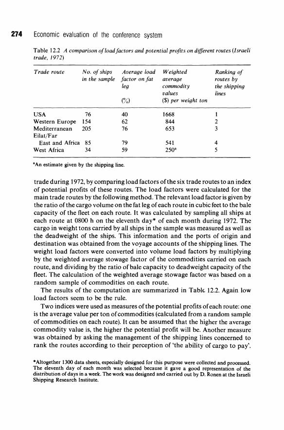
274 Economic evaluation of the conference system
Table 12.2 A comparison of load factors and potential profits on different routes (Israeli trade, 1972)
Trade route No. of ships Average load Weighted Ranking of in the sample factor on fat average routes by
leg commodity the shipping values lines
(%) ($) per weight ton
USA 76 40 1668 1 Western Europe 154 62 844 2 Mediterranean 205 76 653 3 Eilat/Far
East and Africa 85 79 541 4 West Africa 34 59 250' 5
a An estimate given by the shipping line.
trade during 1972, by comparing load factors ofthe six trade routes to an index of potential profits of these routes. The load factors were calculated for the main trade routes by the following method. The relevant load factor is given by the ratio of the cargo volume on the fat leg of each route in cubic feet to the bale capacity of the fleet on each route. It was calculated by sampling all ships at each route at 0800 h on the eleventh day* of each month during 1972. The cargo in weight tons carried by all ships in the sample was measured as well as the deadweight of the ships. This information and the ports of origin and destination was obtained from the voyage accounts of the shipping lines. The weight load factors were converted into volume load factors by multiplying by the weighted average stowage factor of the commodities carried on each route, and dividing by the ratio of bale capacity to deadweight capacity of the fleet. The calculation of the weighted average stowage factor was based on a random sample of commodities on each route. .
The results of the computation are summarized in Tabk 12.2. Again low load factors seem to be the rule.
Two indices were used as measures of the potential profits of each route: one is the average value per ton of commodities (calculated from a random sample of commodities on each route). It can be assumed that the higher the average commodity value is, the higher the potential profit will be. Another measure was obtained by asking the management of the shipping lines concerned to rank the routes according to their perception of 'the ability of cargo to pay'.
* Altogether 1300 data sheets, especially designed for this purpose were collected and processed. The eleventh day of each month was selected because it gave a good representation of the distribution of days in a week. The work was designed and carried out by D. Ronen at the Israeli Shipping Research Institute.
Cartel profits and social costs 275
The ranking of the routes by the shipping lines (column (5» was identical to the ranking according to the average unit value of commodities.
The comparison of the load factor with 'potential profits' of the routes generally proves the point. With the exception of the West African trade route, the load factor increases as trade becomes poorer. Capacity utilization is particularly low on the potentially most rewarding USA route. The West African route has not the highest load factor, in spite of being the potentially least rewarding trade. This route is, however, somewhat exceptional. Most cargo on this route consists oflogs and wood, which are carried under a special contract.
12.4 EXCESSIVE SERVICE COMPETITION
Our model shows that given the price-fixing power of conferences, the expected monopoly profits attract new entrants as well as induces existing firms to expand capacity. The hope of an individual line for a high reward will be frustrated for the very reason that all nourish the same hope. The expected monopoly profits will be wiped out in the end.
In equilibrium when only normal profits are made, and excess capacity exists, a second stage of wasteful competition may take place. Now, every line wants to increase the capacity utilization. Differentiation of services will take place. Each line will offer special qualities to increase its market share, and fill up the empty space. The service competition that follows the creation of excess capacity will tend to raise freight rates still further to compensate for losses made by the least successful of the service-competing conference members. Such competition can rightly be called 'excessive service competition'. The absence of price competition gives shippers no chance of deciding on how much quality of service they are prepared to pay for.
The aspect of excessive service competition that has been paid most attention to is the in optimally high speed of many liner ships. Devanney et al. (1972) for example, have found that the liners on the route between the USA Atlantic coast and the South American Pacific coast have excessive speed - by some 5 knots - from the point of view of shippers' cost minimization. This has contributed to a 25% increase in the freight rates: 'as compared to an efficient system, the present system utilizes 2t times too many ships, which average about a factor of 2 too small and 40% too fast' (Devanney et al., 1972). This figure was obtained by comparing the actual fleet to a simulated efficient one. This estimate may contain an upwards bias of the degree of excess capacity because the load factor of the efficient fleet was unrealistically assumed to be 100%. It is also pointed out that 'similar and indeed greater amounts of overcapacity have been observed in another study on shipping in Latin America' (ECLA, 1968).
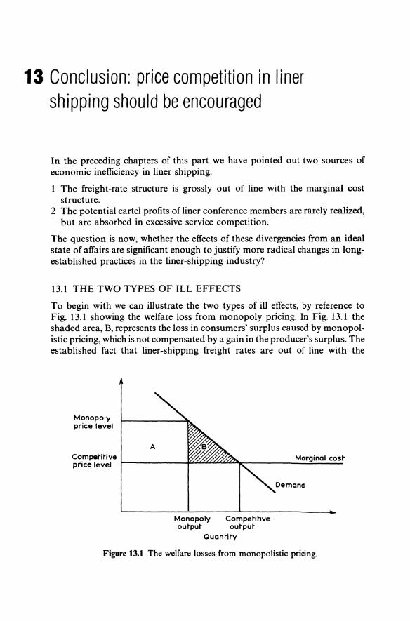
13 Conclusion: price competition in liner shipping should be encouraged
In the preceding chapters of this part we have pointed out two sources of economic inefficiency in liner shipping.
The freight-rate structure is grossly out of line with the marginal cost structure.
2 The potential cartel profits of liner conference members are rarely realized, but are absorbed in excessive service competition.
The question is now, whether the effects of these divergencies from an ideal state of affairs are significant enough to justify more radical changes in longestablished practices in the liner-shipping industry?
13.1 THE TWO TYPES OF ILL EFFECTS
To begin with we can illustrate the two types of ill effects, by reference to Fig. 13.1 showing the welfare loss from monopoly pricing. In Fig. 13.1 the shaded area, B, represents the loss in consumers' surplus caused by monopolistic pricing, which is not compensated by a gain in the producer's surplus. The established fact that liner-shipping freight rates are out of line with the
Monopoly price level
Competitive Marginal cost price level t-------t=""'~"""-"La~-------.:~--.:......:..:~
Monopoly Competitive output output
Quantity
Figure 13.1 The welfare losses from monopolistic pricing.
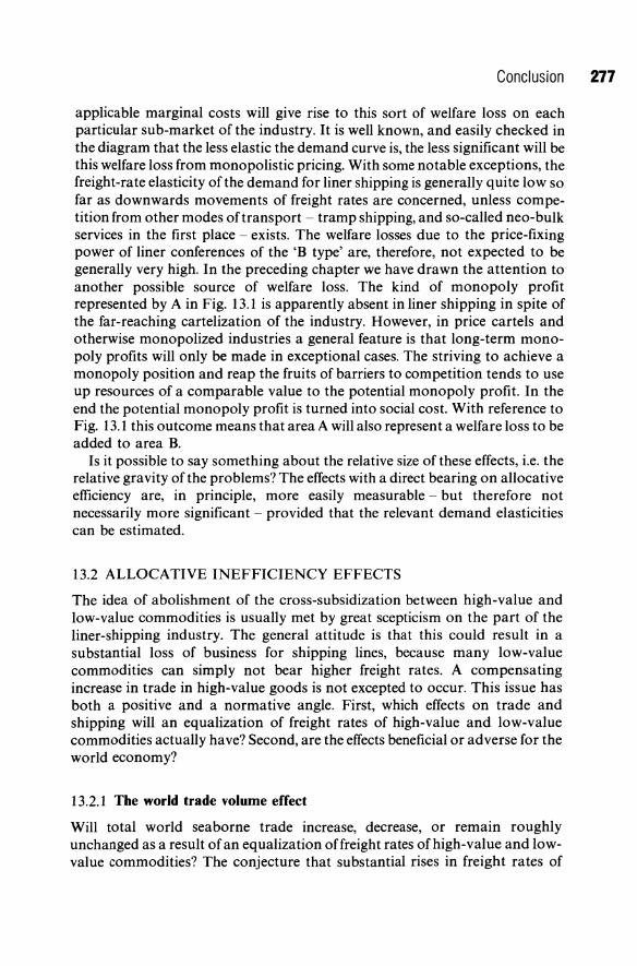
Conclusion 277
applicable marginal costs will give rise to this sort of welfare loss on each particular sub-market of the industry. It is well known, and easily checked in the diagram that the less elastic the demand curve is, the less significant will be this welfare loss from monopolistic pricing. With some notable exceptions, the freight-rate elasticity of the demand for liner shipping is generally quite low so far as downwards movements of freight rates are concerned, unless competition from other modes of transport - tramp shipping, and so-called neo-bulk services in the first place - exists. The welfare losses due to the price-fixing power of liner conferences of the 'B type' are, therefore, not expected to be generally very high. In the preceding chapter we have drawn the attention to another possible source of welfare loss. The kind of monopoly profit represented by A in Fig. 13.1 is apparently absent in liner shipping in spite of the far-reaching cartelization of the industry. However, in price cartels and otherwise monopolized industries a general feature is that long-term monopoly profits will only be made in exceptional cases. The striving to achieve a monopoly position and reap the fruits of barriers to competition tends to use up resources of a comparable value to the potential monopoly profit. In the end the potential monopoly profit is turned into social cost. With reference to Fig. 13.1 this outcome means that area A will also represent a welfare loss to be added to area B.
Is it possible to say something about the relative size of these effects, i.e. the relative gravity of the problems? The effects with a direct bearing on allocative efficiency are, in principle, more easily measurable - but therefore not necessarily more significant - provided that the relevant demand elasticities can be estimated.
13.2 ALLOCA TIVE INEFFICIENCY EFFECTS
The idea of abolishment of the cross-subsidization between high-value and low-value commodities is usually met by great scepticism on the part of the liner-shipping industry. The general attitude is that this could result in a substantial loss of business for shipping lines, because many low-value commodities can simply not bear higher freight rates. A compensating increase in trade in high-value goods is not excepted to occur. This issue has both a positive and a normative angle. First, which effects on trade and shipping will an equalization of freight rates of high-value and low-value commodities actually have? Second, are the effects beneficial or adverse for the world economy?
13.2.1 The world trade volume effect
Will total world seaborne trade increase, decrease, or remain roughly unchanged as a result of an equalization offreight rates of high-value and lowvalue commodities? The conjecture that substantial rises in freight rates of
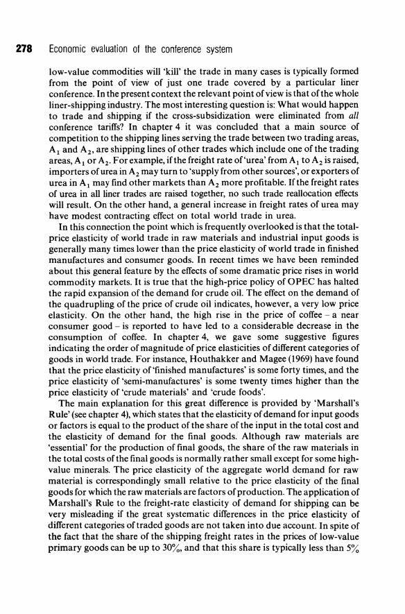
278 Economic evaluation of the conference system
low-value commodities will 'kill' the trade in many cases is typically formed from the point of view of just one trade covered by a particular liner conference. In the present context the relevant point of view is that of the whole liner-shipping industry. The most interesting question is: What would happen to trade and shipping if the cross-subsidization were eliminated from all conference tariffs? In chapter 4 it was concluded that a main source of competition to the shipping lines serving the trade between two trading areas, Al and A2 , are shipping lines of other trades which include one of the trading areas, Al or A2. For example, if the freight rate of , urea' from Al to A2 is raised, importers of urea in A2 may turn to 'supply from other sources', or exporters of urea in Al may find other markets than A2 more profitable. If the freight rates of urea in all liner trades are raised together, no such trade reallocation effects will result. On the other hand, a general increase in freight rates of urea may have modest contracting effect on total world trade in urea.
In this connection the point which is frequently overlooked is that the totalprice elasticity of world trade in raw materials and industrial input goods is generally many times lower than the price elasticity of world trade in finished manufactures and consumer goods. In recent times we have been reminded about this general feature by the effects of some dramatic price rises in world commodity markets. It is true that the high-price policy of OPEC has halted the rapid expansion of the demand for crude oil. The effect on the demand of the quadrupling of the price of crude oil indicates, however, a very low price elasticity. On the other hand, the high rise in the price of coffee - a near consumer good - is reported to have led to a considerable decrease in the consumption of coffee. In chapter 4, we gave some suggestive figures indicating the order of magnitude of price elasticities of different categories of goods in world trade. For instance, Houthakker and Magee (1969) have found that the price elasticity of 'finished manufactures' is some forty times, and the price elasticity of 'semi-manufactures' is some twenty times higher than the price elasticity of 'crude materials' and 'crude foods'.
The main explanation for this great difference is provided by 'Marshall's Rule' (see chapter 4), which states that the elasticity of demand for input goods or factors is equal to the product of the share of the input in the total cost and the elasticity of demand for the final goods. Although raw materials are 'essential' for the production of final goods, the share of the raw materials in the total costs ofthe final goods is normally rather small except for some highvalue minerals. The price elasticity of the aggregate world demand for raw material is correspondingly small relative to the price elasticity of the final goods for which the raw materials are factors of production. The application of Marshall's Rule to the freight-rate elasticity of demand for shipping can be very misleading if the great systematic differences in the price elasticity of different categories of traded goods are not taken into due account. In spite of the fact that the share of the shipping freight rates in the prices of low-value primary goods can be up to 30%, and that this share is typically less than 5%
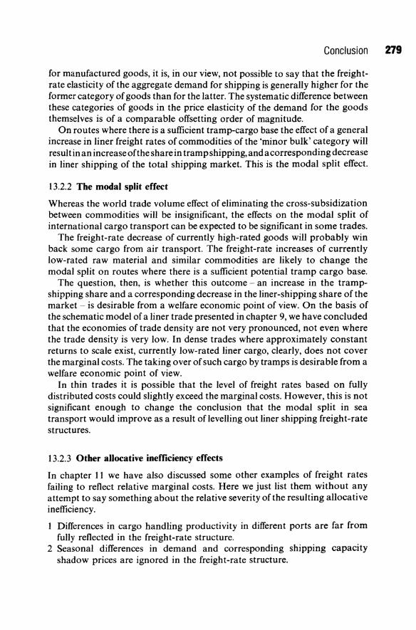
Conclusion 279
for manufactured goods, it is, in our view, not possible to say that the freightrate elasticity of the aggregate demand for shipping is generally higher for the former category of goods than for the latter. The systematic difference between these categories of goods in the price elasticity of the demand for the goods themselves is of a comparable offsetting order of magnitude.
On routes where there is a sufficient tramp-cargo base the effect of a general increase in liner freight rates of commodities of the 'minor bulk' category will result in an increase ofthe share in tramp shipping, and a corresponding decrease in liner shipping of the total shipping market. This is the modal split effect.
13.2.2 The modal split effect
Whereas the world trade volume effect of eliminating the cross-subsidization between commodities will be insignificant, the effects on the modal split of international cargo transport can be expected to be significant in some trades.
The freight-rate decrease of currently high-rated goods will probably win back some cargo from air transport. The freight-rate increases of currently low-rated raw material and similar commodities are likely to change the modal split on routes where there is a sufficient potential tramp cargo base.
The question, then, is whether this outcome - an increase in the trampshipping share and a corresponding decrease in the liner-shipping share of the market - is desirable from a welfare economic point of view. On the basis of the schematic model of a liner trade presented in chapter 9, we have concluded that the economies of trade density are not very pronounced, not even where the trade density is very low. In dense trades where approximately constant returns to scale exist, currently low-rated liner cargo, clearly, does not cover the marginal costs. The taking over of such cargo by tramps is desirable from a welfare economic point of view.
In thin trades it is possible that the level of freight rates based on fully distributed costs could slightly exceed the marginal costs. However, this is not significant enough to change the conclusion that the modal split in sea transport would improve as a result oflevelling out liner shipping freight-rate structures.
13.2.3 Other allocative inefficiency effects
In chapter 11 we have also discussed some other examples of freight rates failing to reflect relative marginal costs. Here we just list them without any attempt to say something about the relative severity of the resulting allocative inefficiency.
Differences in cargo handling productivity in different ports are far from fully reflected in the freight-rate structure.
2 Seasonal differences in demand and corresponding shipping capacity shadow prices are ignored in the freight-rate structure.
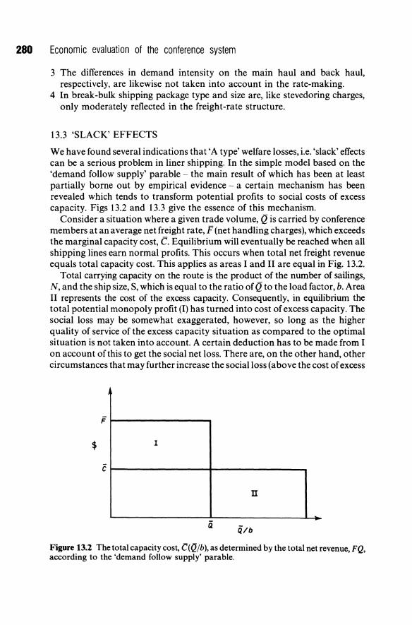
280 Economic evaluation of the conference system
3 The differences in demand intensity on the main haul and back haul, respectively, are likewise not taken into account in the rate-making.
4 In break-bulk shipping package type and size are, like stevedoring charges, only moderately reflected in the freight-rate structure.
13.3 'SLACK' EFFECTS
We have found several indications that 'A type' welfare losses, i.e. 'slack' effects can be a serious problem in liner shipping. In the simple model based on the 'demand follow supply' parable - the main result of which has been at least partially borne out by empirical evidence - a certain mechanism has been revealed which tends to transform potential profits to social costs of excess capacity. Figs 13.2 and 13.3 give the essence of this mechanism.
Consider a situation where a given trade volume, Q is carried by conference members at an average net freight rate, F (net handling charges), which exceeds the marginal capacity cost, C. Equilibrium will eventually be reached when all shipping lines earn normal profits. This occurs when total net freight revenue equals total capacity cost. This applies as areas I and II are equal in Fig. 13.2.
Total carrying capacity on the route is the product of the number of sailings, N, and the ship size, S, which is equal to the ratio of Q to the load factor, b. Area II represents the cost of the excess capacity. Consequently, in equilibrium the total potential monopoly profit (I) has turned into cost of excess capacity. The social loss may be somewhat exaggerated, however, so long as the higher quality of service of the excess capacity situation as compared to the optimal situation is not taken into account. A certain deduction has to be made from I on account of this to get the social net loss. There are, on the other hand, other circumstances that may further increase the social loss (above the cost of excess
F ~----------------~
$ I
c ~-----------------+----------------~
II
a
Figure 13.2 The total capacity cost, C( (JIb), as determined by the total net revenue, FQ, according to the 'demand follow supply' parable.

Conclusion 281
F ~ ________ ..,
$ I
C~------------r------------r----, II I I
I I
" l I F ~-------------~! -------.-.I----t,
Q+Q
~i~ure 1~.3 The total capacity cost, C(Q + Q), as determined by the total net revenue, FQ + PQ, according to the 'demand follow supply' parable incorporating the possibility to lift filling cargo.
capacity). If the capacity costs of the conference members are different, the level offreight rates will be such that the high-cost lines think it isjust worthwhile to continue operating in the trade. In this case the cost of the excess capacity underrates the possible shipping-cost savings. An additional possibility to reduce costs is that the most efficient lines outcompete (in price) the inefficient ones with the result that the mean level of capacity costs is lowered.
Expansion into the tramp market will not reduce these losses. The average level of tramp rates, ft, is typically well below C, but of course, positive (otherwise filling cargo would not interest liners). Assuming that all sailings on the route are now filled up, the total net revenue area takes the shape shown in Fig. 13.3.
A 'tail' of thickness ft is added to the total net revenue area. The length ofthe tail is determined by the additional quantity of filling cargo, Q, which is obtained in the tramp-shipping market. The total sailings is now No which exceeds sailings in the original situation, where no filling cargo was available. The areas I and II are the same as those of Fig. 13.2. In equilibrium (where no more than normal profits are made) area II has to equal area I. This condition determines the value of Q. The end result is apparently that the magnitude of the social loss remains the same as in the original situation.
13.4 ENCOURAGE PRICE COMPETITION AND SERVICE COORDINA TION
What can be done about the wasteful practices? If the freight-rate structure were brought in line with the marginal-cost structure, an important precondition for the elimination of the problem would be present. Not only would
282 Economic evaluation of the conference system
allocative efficiency in world trade and shipping be enhanced, but also the wasteful rivalry for the coveted high-rated commodities would disappear.
Is it likely that conferences would voluntarily adopt a fully cost-based tariff, and give up the possibility to charge what the traffic can bear? No, to believe that is wishful thinking. Freight-rate discrimination is a means of more than 100 years standing to increase revenue, and, furthermore, liner conference ratemakers are under the 'common-costs illusion'; all freight rates which exceed the direct handling costs are considered to be profitable. This means that there is no incentive even to raise the freight rates ofloss-making cargo to the level of the true marginal costs.
The only sure policy for elimination of the freight-rate discrimination would be the abolishment of liner conferences as price cartels. This has to be done both by enforcement of new laws, and by encouragement of competition. It is not enough that a regulatory authority tells cartels how to set prices; it has also to ensure that conference members do not prevent individual members pursuing their own pricing policy, i.e. that they do not behave as a price cartel. If that is achieved, price competition within the conference will be introduced. Only real price competition would make the structure of freight rates fully in line with the marginal cost structure.
13.4.1 Exposure of the common-cost illusion
We predicted that price competition would expose the common-cost illusion. With the present conference system the existence of high-rated commodities invites the belief that low-rated commodities (with freight rates below the marginal costs but above the direct handling costs) are profitable, too. Operators tend to think in terms of full shiploads. If a particular commodity moves in a quantity which is insufficient to fill a ship - very few commodities carried by liners move in such large quantities - no capacity costs should be attributed to the commodity in question according to the current thinking. If the freight rates of low-rated commodities exceed the direct handling costs, low-rated commodities will not be rejected, because together with the highrated commodities which will be included in the same shipload, they will contribute to the net profit.
Suppose, however, that the price cartels are dissolved. Competition for the high-rated cargo will then be fierce. The high rates will soon be bid down, and the result would be an equalization of the net marginal revenue of all commodities. Different shipping lines serving the same trade are generally very close substitutes. This means that the freight-rate elasticity of demand of different articles will from the point of view of an individual shipping line appear by and large the same, i.e. very high for all commodities. (This is, of course, not inconsistent with the conference, as a collective body, viewing some commodities as possessing a low elasticity of demand and some commodities as possessing a high elasticity of demand.) This in turn means that the

Conclusion 283
'contribution margin', to talk in cost accounting terms, will be more or less the same for all commodities.
In this situation every article which does not bear its share of the capacity costs will be considered to be loss making since there are no articles to be obtained with compensating, disproportionately high contribution margins.
13.4.2 Will the liner freight rate stability come to an end?
Wide fluctuations of freight rates, even in the short term, are feared by defenders of the conference system to occur if price competition is set free. Many vivid examples of this are to be found in bulk shipping markets. It is unlikely, however, that the short-term ups and downs of tramp freight rates will be copied in liner shipping.
One quality ofliner-shipping services is that the freight rates that will apply at future dates are known by shippers fairly well in advance. The idea of a tariff is that reliable freight-rate information should be available for everybody concerned to facilitate shipment planning for the shippers. This quality of service should be maintained also after setting price-competition free. The service of a shipping line that cannot say in advance what the freight rates will be, would be considered inferior to the services of shipping lines that issue tariffs valid for a considerable period of time ahead. The prevailing period of notice of freight-rate changes should continue to be applied after the introduction of price competition.
A tariff ofthis kind has necessarily to be based on expected costs for a future period of time of some duration. The actual cost of taking on additional cargo on a particular sailing is widely fluctuating. It is frequently almost as low as the direct handling costs, but occasionally it can be very high. The expected cost of additional cargo is an entirely different matter. Over a longer period of time the short-run expected marginal cost will be nearly equal to the total average cost, provided that the liner-service operators make rational decisions about ship and service design. The relevant expected cost when it comes to freightrate making is in the first place determined by the total demand relative to offered capacity of the period of time during which the freight rates ofthe tariff are given. This means that notwithstanding short-term fluctuations in demand (from one sailing to another) reasonable price stability is likely to characterize liner shipping also in the absence of the price cartels. Liner conferences may well continue to produce freight-rate tariffs as 'guidelines' for individual members also in a situation where individual shipping lines/conference members are at liberty to charge their own rates. This may have a stabilizing influence on freight rates. Finally, it should be remembered that even under the current conference umbrella rates do fluctuate in the face of outside competition (section 3.1), certainly more than is apparent by the publicly announced rate changes.
284 Economic evaluation of the conference system
13.4.3 A new role for liner conferences
If liner conference tariffs were to be regarded just as lists of 'recommended prices', what would then be the real raison d'etre of the conferences? Would they then be largely superfluous? The answer is definitely in the negative. Liner conferences have a very important task to fulfil in the coordination of schedules and sailings in each particular trade. As has been argued in a number of previous places, the quality of service in liner trade is to a high degree a collective characteristic of the supply of all shipping lines taken together. The frequency of sailings is the most important aspect, but also the ports of call at each end of the route in question, and the organization of feeder services are matters of great concern for shippers, which are difficult to settle in a satisfactory way without coordination of the actions of individual shipping lines. The schematic liner-trade model of chapter 9 is an illustration of how both user (shippers') costs and the producer costs of the total supply of liner shipping on a particular route should be taken into account in order to carry out the liner service optimization necessary for overall economic efficiency. It is difficult to imagine that this could be obtained even very approximately without fairly close coordination of schedules and itineraries of individual shipping lines. The liner conferences seem to be the natural bodies for this coordination.
At first, it may appear incompatible that the conference members coordinate their sailings etc. for social-cost minimization on the one hand, and enter into price competition with each other, on the other. On second thoughts, however, such seemingly inconsistent behaviour may not be unrealistic at all. Price competition basically means that individual producers/sellers are not prevented from changing their prices, when they consider it profitable, not that very frequent price changes actually take place. Oligopolistic markets similar to a typical liner trade are not characterized by widely dispersed inter-firm price structures, or frequent price changes. On the contrary, equality of prices and price stability are the salient features. So in these respects everything would most likely look pretty much the same after as before the abolishment of restrictions on the pricing policy of individual shipping lines. However, the very fact that any individual line which has obtained a cost advantage over its competitors/fellow conference members, can lower (or, more likely in these days raise by a smaller amount) the price would have a healthy influence on incentives and behaviours of liner-shipping companies.
13.4.4 Assisting the 'invisible hand'
In this connection we want to stress again how important it is for the success of such a new competitive regime that the grossly discriminatory structure of freight rates in present tariffs is eliminated. As long as there remains very profitable cargo as well as moderately profitable and unprofitable cargo, the system would be exposed to strains, which may be too strong for its survival.
Conclusion 285
We have said before that price competition would tend to equalize contribution margins, making all cargo equally (moderately) profitable. However, given the extremely large disparities in contribution margins in the initial position, it may be too much to ask offree price competition to expect that an orderly approaching of the freight rates to the corresponding marginal costs would occur automatically. A helping hand may be needed (in addition to the 'invisible' one) in the form of guidelines issued by an independent (presumably) governmental regulatory body. These guidelines could take the form of the principles outlined in chapter 11 of cost-based freight-rate tariffs.
13.5 RECENT ATTEMPTS OF REFORMING LINER CONFERENCE PRACTICES
Just as we have argued above the report of the British inquiry into shipping (the Rochdale Report, 1970) concluded that economic efficiency requires coordination of services, which cannot be obtained otherwise than by collective decisions by liner conferences. To safeguard against the risk that the 'closed conferences' approved of per se results in too quiet a life for individual members/shipping lines and consequent slackness and inadequate cost consciousness, the committee sensibly pointed out that the admission of new members should not be decided just by the existing conference members: 'Applications from liner operators to become members of a conference ... which cannot be settled by negotiation between existing members and the applicant, should be referred, if the applicant so requested, for adjudication to a panel with an independent chairman on which shippers have representation' (Rochdale Report, 1970; p. 135).
As to the pricing policy of liner conferences, the committee did not go into the details of the freight-rate structure versus the marginal cost structure, but seemed to be concerned mainly with the total cost and revenue ofliner services on different routes; however, it strongly recommended that tariffs 'should be published and available to anybody on request at reasonable cost' (Rochdale Report, 1970; p. 135).On the crucial matter of whether or not the price cartels are a desirable aspect of liner conferences, the committee nowhere explicitly takes a clear stand. Indirectly it can be inferred that the committee took for granted that if conference members are to coordinate sailings, they should also be allowed to agree on freight rates, iffor no other reason, because it may seem impractical to stop them from doing so under this condition.
The USA Shipping Act, 1984 makes a definite exemption of liner shipping from anti-trust laws. On the other hand, a completely new provision is that individual shipping lines are legally sanctioned to charge freight rates which are different from those 'recommended' by the conference. In our view this represents a modern approach to competition policy. It has always been difficult to enforce price-cartel prohibitions. Secret agreements between the producers of a particular product to charge the same price is hard to detect,

286 Economic evaluation of the conference system
especially if the agreement has the character of a mutual 'understanding' that a common pricing policy is to be followed. If potential competitors do not want to compete on price, no government or regulatory authority can force them to do so. Legislation can be much more effective by directing itself to the protection of those who want and dare to pursue an individual pricing policy.
At the time of writing it is difficult to predict how important this change of direction in USA regulatory policy will be in practice in the future. Will it turn out to be true that, as the president of Farrell Lines put it in a recent symposium on new challenges for shipping and ports, 'ocean carriers now move into an era of less government but more marketplace regulation'? (Parks, 1984; p. 147).
13.6 PROBLEMS OF REGULATING INTERNATIONAL LINER SHIPPING
The code ofliner-conference practice in the Rochdale Report was produced to 'safeguard our (British) immediate national interest' (p. 135). It was at the same time recognized that the whole issue had very wide international implications. Since few major trades are served by ships of just one nation if other governments were to impose markedly different and conflicting codes, liner conferences could be faced with a very complicated situation. Therefore the Rochdale committee came up with the interesting idea, with a clear address to shipowners all over the world, that since it is very likely that other governments sooner or later will seek to impose codes of conduct on shipping companies in liner conferences, the wisest step that shipowners could take, would be to agree among themselves on a code of conduct, which (hopefully) would be based on the Rochdale proposals.
According to a later account (UWIST, 1982) by Professor R. Goss, economic adviser to the Rochdale committee, of what followed after the report had been submitted, numerous and lengthy discussions took place on the implementation ofthe code of conduct proposed by the committee. Eventually the Committee of European National Shipowners' Association (including Japanese shipowners) drew up a sort of code of liner conference practice (the 'CENSA Code' of 1972). However, in relation to the Rochdale proposal, it was, in the words of Richard Goss, considerably watered down, in that, for example:
Admission arrangements were weaker, being subject only to the control of shipowners.
2 Tariffs were to be made available to shippers' organizations but not published.
3 Governments were not to be involved.
As a matter of fact the CENSA Code was basically an endorsement of the
Conclusion 287
status quo, and, in particular, it failed to adopt any of the reforms suggested by the Rochdale Committee. 'There must, of course, be some understandable suspicion that a voluntary code produced by the proponents of cartels may tend to be less effective than such a Committee as that chaired by Lord Rochdale would have wished' to quote a typical understatement by Richard Goss.
The main stumbling block is, of course, the notorious problem of regulating an international industry like the liner-shipping industry. Is it at all likely that a code ofliner conference practice, which is designed from the point of view of one particular nation, could be acceptable from a global point of view, or, at least to the other nations concerned involved in the liner shipping, either as exporters/importers of liner cargo, or as suppliers of liner-shipping services? The approach of the Rochdale Committee seemed to begin with rather promising thoughts in this regard thanks to its objectivity and independence. The timing was unfortunate, the report came too late. At that time other forces were gaining momentum in the liner-shipping world. The problems of international agreement on a code of liner-conference practice obviously become aggravated when nations attempt to further other interests than economic efficiency by means ofliner-shipping regulation. This is exactly what happened, and it has caused much controversy and confusion. Certain developing countries have been pressing forward through UNCT AD a code of conduct for liner shipping, which obviously has promotion of their national fleets rather than an economical division of labour in international liner shipping as its primary aim.
13.7 HOPES FOR THE FUTURE
It is, of course, pointless to regret that not just economic efficiency is a goal of national shipping policy. In the present circumstances the only thing one can hope for is that the different issues do not become too blurred and confused. Our recommendation has 'global economic efficiency' as its guiding star, and we mean that it need not be in very serious conflict with various other national ambitions. After all, the liner-trade volume affected by the cargo-sharing guidelines of the UNCT AD code is no more than about 7% of the total trade carried by international liner shipping.
A potentially more interesting event on the international liner shipping scene from an economic point of view is the many new entries of shipping companies from emerging shipping nations, as well as the beginning disintegration of many liner conferences. In recent years a number of major liner-trade routes have to an increasing extent been served by independent shipping lines operating outside the conferences. This has worked without very dramatic upheavals. Profits have been low in liner shipping, but this is mainly due to the over-tonnaging created by the over-optimistic container ship

288 Economic evaluation of the conference system
investments in the 1970s (in the prolonged period of shipyard 'sale'). Freight rates should be low in such a situation, in order to help a new equilibrium emerge as quickly as possible.
We are witnessing the last phases of both a technological transformation of traditional break-bulk cargo shipping, and a change of roles on the scenes of international shipping between old shipping lines of the traditional shipping nations, and new entries, which now have learnt the technique of unit-load sea transport, and still have wages at levels far below the USA and the European countries. Conference resistance to freer price competition may retard these changes, but this is not worth endorsing by governments of the declining shipping nations. The best division of labour in international sea transport is obtained when the most efficient operators become price leaders. The USA Shipping Act, 1984 is the first important governmental step towards price competition in liner shipping. Let us hope that other shipping nations will follow suit.

References
Abrahamsson, B.J. (1968) A model of liner price setting. Journal of Transport Economics and Policy, September.
Ahle, T. et al. (1977) Sjoterminaler for Enhetslasttrajik, Kjessler and Mannerstrale AB, Stockholm.
Allen, R.G.D. (1975) Index Number in Theory and Practice, Macmillan, London. Australian Department of Transport (1977) Report on a Review of Overseas Cargo
Shipping Legislation, October. Balassa, B. and Kreinin, M. (1967) Trade liberalization under the Kennedy round, The
Review of Economics and Statistics, May. Baumol, W.S. and Vinod, H.D. (1970) An inventory theoretical model of freight
transport demand. Management Science, March. Benford, H. (1968) General Cargo Ship Economics and Design, College ot Engineering,
University of Michigan. Bennathan, E. and Walters, A.A (1969) The Economics of Ocean Freight Rates, Praeger,
New York. Bennathan, E. and Walters, A.A. (1983) Port Pricing and Investment in Developing
Countries, a World Bank research publication, Oxford University Press, Oxford.
British Transport Docks Board (1967) Containerization: The Key to Low-Cost Transportation. Report by McKinsey & Co., Ltd.
Bryan, A.1. (1974) Regression analysis of ocean freight rates on some Canadian export routes. Journal of Transport Economics and Policy, May.
Bryan, A.1. and Cape, D.M. (1982) Liner Conference Freight Index for Canadian Exports, Canadian Transport Commission, Research Branch, Report No. 1982jOIE, January.
Buss, G. Stowage Factors for all Kinds of Merchandise (compiled by Captain O. Stahlbaum and W. Moth), Verlag OKIS, Hamburg.
Buxton, I.L. (1971) Engineering Economics and Ship Design, The British Ship Research Association, Wallsend.
Buxton, I.L., Daggit, R.P. and King, J. (1978) Cargo Access Equipment for Merchant Ships, E. & F.N. Spon, London.
Central Bureau of Statistics (1975-84) The national accounts of Israel. Monthly Bulletin of Statistics.
Chapman, K.R. (1969) Estimation of Characteristics of Cellular Container Vessels, University of Newcastle, Newcastle.
Chinitz, B. (1956) Rate discrimination in ocean transport, PhD dissertation, Harvard University.
Croner's World Directory of Liner Conferences (1976), Compiled and edited by R.K. Bridges, Croner Publications Ltd, New Malden, Surrey.
Deakin, B.M. in collaboration with T. Seward (1973) Shipping Conferences. A Study of their Origins. Development and Economic Practices, University of Cambridge, Dept. of Applied Economics, Occasional Paper 37, Cambridge University Press, Cambridge.
290 References
Devanney, III, J.W., Livanos, V.M. and Stewart, RJ. (1972) Conference Rate-making and West Coast of South America, Commodity Transportation and Economic Development Laboratory, MIT Press, Chicago.
ECLA (1968) Maritime Freight Rates in the Foreign Trade of Latin America. Economic Commission for Latin America E/CN 12/812/Rev 1. 24 November.
ECLA (1968) Special studies on Latin America, Part 3. Recent Trends in Latin America Maritime Transport, Economic Commission for Latin America, E/CN 12/851, chapter 3.
EEC Regulation 954/79 Erichsen, S. (1971) Optimum Capacity of Ships and Port Terminals, College of
Engineering, University of Michigan. Evans, J.J. (1977) Liner freight rates discrimination and cross-subsidization. Maritime
Policy and Management, 4, 41. Evens., J.J. (1982) Concering the level of line's freight rates. Martime Policy and
Management, 2. Fact Finding Investigation (1961) No.6: The Effects of Steamship Coriference
Organization, Procedure, Rules and Practices upon the Foreign Commerce of the United States, FMC, Washington D.C.
Federal Maritime Commission (1968) Investigation of Ocean Rate Structures in the Trade between US North Atlantic Ports and Ports in UK and Eire. Docket No. 64-65. (Decision 14 August 1968.)
Ferguson, A.R., Allen, R., Lerner, E.M., McGee, J.S., Oi, W.Y., Rapping, L.A. and Sobotka, S.P. (1961) The Economic Value of the United States Merchant Marine, The Transportation Center, Northwest University, Evanston, USA.
Foster, C.D. (1975) The Transport Problem, 2nd rev. edn, Croom Helm, London. Friedmann, P.A. and Devierno, J.A. (1984) The Shipping Act of 1984: The shift from
government regulation to shipper regulation. Journal of Maritime Law and Commerce, July.
Gardner, B. (1978) An alternative model of price determination in liner shipping. Maritime Policy and Management, 3.
Gedda, S. and Kock, A. (1966) Principer for fralsstiittning vid sjotrausport av container. Skips fartsokonomisk Institutt, Bergen.
Getz, J.R., Erichsen, S. and Heirung, E. (1967) Design of a Cargo Liner in Light of the Development of General Cargo Transportation, Society of Naval Architects and Marine Engineers, U.S.A.
Gilman, S. (1977) Shipping technologies for developing countries. Journal of Transport Economics and Policy, January.
Gilman, S. (1983) In Containers and their Competitors, Marine Transport Centre, Liverpool University, Liverpool.
Goss, RO. (1968) Studies in Maritime Economics, Cambridge University Press, Cambridge.
Goss, RO. (ed.) (1970) In The Feature of European Ports, College of Europe, Burges. Goss, RO. and Jones, C.D. (1971) The Economies of Size in Dry Bulk Carriers, HMSO,
London. Goto, S. (1983) In International Symposium on Liner Shipping I II. Bremen, 1-3
November 1983. Haldi, J. and Whitcomb, D. (1967) Economies of scale in industrial plants. Journal of
Political Economy, August.
References 291
Heaver, T. (1968) The Economies of Vessel Size: A Study of Shipping Costs and their Implications to Port Investments, National Harbour Board, Ottawa.
Heaver, T. (1973) A theory of shipping conference pricing and policies. Maritime Studies and Management, 1.
Heaver, T.D. (1972) Trans Pacific trade, liner shipping and conference rates. Logistics and Transportation Review, 8, 2.
Heggie, I. (1974) Charging for port facilities. Journal of Transport Economics and Policy, January.
HMSO (1970) Report by Committee of Enquiry into Shipping, HMSO, London. Houthakker, H.S. and Magee, S. (1969) Income and price elasticities in world trade.
Review of Economics and Statistics, May. Jansson, J.O. (1974) Intratariff cross-subsidization in liner shipping. Journal of
Transport Economics and Policy, September. Jannson, J.O. and Shneerson, D. (1982) Port Economics, MIT Press, Chicago. Johanson, L. (1972) Production Functions, North Holland, Amsterdam. Johnson, E.R. and Huebner, G.G. (1960) Principles of Ocean Transportation, Appleton
Co. New York. Johnson, K.M. and Garnett, H.S. (1971) The Economics of Containerization, University
of Glasgow Social and Economic Studies, 20, George Allen and Unwin, London.
Kendall, M.G. (1968) Liner Freight Index, UNCTAD TD/29, January. Kendall, P.M. (1972) The theory of optimal ship size. Journal of Transport Economics
and Policy, May. Koiki, Y. (1975) in Containers and their Competitors (ed. E.T. Laing), Marine Transport
Centre, Liverpool University, Liverpool. Laing, E.T. (1975) in Containers and their Competitors, Marine Transport Centre,
Liverpool University, Liverpool. Laing, E.T. (1975/76) Tho:: rationality of conference pricing and output policies.
Maritime Policy and Management, 3. Lawrence, S.A. (1972) International Sea Transport: The Years Ahead, Lexington
Books, USA. Locklin, D.P. (1972) The Economics of Transportation, 7th edn (eds I. Homewood and
R.D. Irwin), Chicago. McCaul, J.B. (1970) Air cargo and ocean shipping industry. Paper presented at a
meeting of the New York Metropolitan Section of Naval Architects and Marine Engineers, 22 September.
McLachlan, D.L. (1958) Index numbers of linerfreight rates in UK trades 1946-1957. Yorkshire Bulletin of Economic and Social Research, June.
McLachlan, D.L. (1963) Pricing of Ocean Transportation, PhD dissertation, University of Leeds.
Madden, W.J. (1970) Import, export air cargo highest ever through PA. Newark StarLedger, 21 May.
Matthews, S.J. (1984) North Europe/East Med. carriers halt the rate slide. Containerization International, November.
Meusen, P. (1971) Handling of Container Vessels Beyond the Third Generation, Port of Rotterdam.
Parks, R.V. (1984) in International Symposium: New Challenge for Shipping and Ports, Israel Shipping and Aviation Research Institute, Haifa.
292 References
Posner, R.A. (1975) The social costs of monopoly and regulation. Journal of Political Economy, 83, 4.
Rath, E. (1973) Container Systems, John Wiley, New York. Robinson, R. (1978) The size of vessel and turnaround times. Journal of Transport
Economics and Policy, XII. Rochdale Report (1970), Committee of Enquiry into Shipping, Chairman V.R. Rochdale,
May, Cmnd 4387, HMSO, London. Ross-Bell, I. (1984) International Symposium: New Challenges for Shipping and Ports,
Israel Shipping and Aviation Research Institute, Haifa. Shear, Admiral H.E. (1983) In International Symposium on Liner Shipping III, Bremen,
1-3 November. Shipping Act, 1984, Public Law 98-237, 98th Congress, Washington. Shneerson, D. (1976) The structure of liner freight rates - a comparative route study.
Journal of Transport Economics and Policy, January. Sletmo, G.K. (1972) Demand for Air Cargo, Institute for Shipping Research. The
Norwegian School of Economics and Business Administration, Bergen. Sletmo, G.K., and Williams, E.W. (1981) Liner Conferences in the Container Age,
Macmillan Publishing Co. Inc., New York. Sturmey, S.G. (1967) Economics and liner services. Journal of Transport Economics and
Policy, May. Swedish Shipping Gazette (1976) 52 (Sjofartens Bok 1977) Thomas, R.E., Captain (1968) Stowage: The properties and stowage of cargoes, Brown,
Son and Ferguson Ltd, Glasgow. Thorburn, T, (1960) Supply and Demand of Water Transport, EFI, Stockholm. UNCTAD (1969) The Liner Trade Between France and Morroco, TD/B/C.4/38, Rev.
2, New York. UNCTAD (1970) Consultation in Shipping, second report, TIBC.4/78, UNCTAD
Secretariat, New York. UNCTAD (1970) Level and Structure of Freight Rates. The Liner Trades Between
France (Bayonne-Dunkirk range of ports) and Morroco, TD/B/C. 4/61. January, UNCTAD Secretariat, New York.
US Department of Commerce (1972) A Neo-Bulk Shipping Study, Harbridge House Inc., Washington D.C.
UWIST (1982) Shipping and Competition Policy, Department of Maritime Studies, University of Wales, Cardiff.
Walters, A.A. (1968) The Economics of Road User Charges, World Bank Occasional Paper No.5.
Waters, W.G. II, (1972), Transport Costs, tariffs and the pattern of industrial protection, American Economic Review.
Wei, V., Kurasawa, H., Hennessy, B. and Fortier, S. (1983) Shipping Conference Freight Indicesfor Canadian Export Trade (1978-1981), Canadian Transport Commission Research Branch, Report No. 1984/01, June.
Yance, J.Y. (1972) Non-price competition in jet aircraft capacity. Journal of Industrial Economics, 1, 55-71.
Zerby, J.A. and Conlon, R.M. (1982) Liner costs and pricing policies. Maritime Policy and Management, 9,3.
Author index
Abrahamsson, B.J. 70, 219 Ahle, T. 113 Allen, R.G.D. 55
Balassa, B. 98 Baumol, W.S. 210 Benford, H. 113, 130 Bennathan, E. ix, 78, 95, 202 Bryan, A.I. 72 Buss, G. 78 Buxton, I.L. 113
Chapman, K.R. 130 Chinitz, B. 72
Deakin, B.M. ix, 1,42, 49, 50~51, 66 Devanney, III, J.W. 221, 275
ECLA, Economic Commission for Latin America 72
Erichsen, S. 113, 130, 131 Evans, 70, 219
Ferguson, A.R. 220~21 Foster, CD. 70 Friedman, P.A. 44
Gardner, B. 70, 219 Gedda, S. 70, 219 Gilman, S. 70, 113, 219 Goss, R.D. ix, 113, 131, 135, 137~38,
202,286
Heaver, T. 70, 72~73, 113, 135,219 Heggie, I. 201 Houthakker, H.S. 98, 278
Jansson, J.O. 78, 80, 203, 219, 238, 242 Johanson, L. 151
Johnson, E.R. 37 Johnson, K.M. 158
Kendall, M.G. 52 Kendall, P.M. 113 Koike, Y. 28,39
Laing, E.T. 31, 70, 113,219 Lawrence, S.A. 21, 31, 32, 33 Locklin, D.P. 70
McLachlan, D.I. 38,49,51,66 Magee, S. 98, 278 Matthews, SJ. 54 Meusen, P. I99~200
Parks, R.V. 286 Posner, R.A. 264
Rath, E. 199-200 Robinson, R. 126 Rochdale, V. 37, 44, 285, 287 Ronen, R. 275 Ross-Bell, I. 46
Shear, Admiral 15 Shneerson, D. 72~ 73, 78, 80, 203, 238,
242 Sletmo, G.K. ix, 95 Stromme-Svendsen, A. ix Sturmly, S.G. ix, 70, 219
Thorburn, T. ix, 123-24, 127, 128, 135, 144,252
UNCTAD, United Nations Conference for Trade and Development 72, 78, 133

294 Author index
Walters, A.A. ix, 78, 95, 202 Waters, W.G. 70 Wei, V. 52, 53 Whitcomb, D. 115
Williams, E.W. ix, 95
Vance, J.V. 270
Zerby, J.A. 70, 219
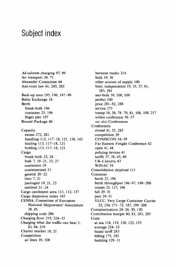
Subject index
Ad-valorem charging 97, 99 Air transport 39, 71 Alexander Committee 44 Anti-trust law 41, 245, 285
Back-up area 195, 196, 197-99 Baltic Exchange 18 Berth
break -bulk 196 container 25, 196 finger pier 197
Brussel Package 46
Capacity excess 272, 281 handling 113, 117-18, 121, 138, 142 hauling 113, 117-18, 121 holding 113, 117-18, 121
Cargo break-bulk 23, 24 bulk 7, 18-21, 23, 27 containers 19 containerized 31 general 20-22 liner 7, 21 packaged 19, 21, 23 unitized 21-24
Cargo catchment area Ill, 112, 157 Cargo dispersion index 165 CENSA, Committee of European
National Shipowners' Association 38,45
shipping code 286 Charging floor 219, 224-25 Charging what the traffic can bear 1,
83,94, 219 Charter market 18,21 Competition
air lines 39, 108
between trades 214 bulk 19,38 other sources of supply 100 liner, independents 19, 55, 57, 81,
283,284 neo-bulk 39, 108, 109 perfect 100 price 281-82, 288 service 275 tramp 18,38,78-79,81, 108, 109,217 within conference 56-57 see also Conferences
Conferences closed 41, 55, 285 competition 39 CONISCON 54-59 Far Eastern Freight Conference 42 open 41, 44 policing devices 41 tariffs 37, 38, 45, 49 UK-Calcutta 43 WINAC 54
Consolidation shipload III Container
berth 25, 196 berth throughput 196-97, 199-200 cranes 25, 127, 196 full 29-31 part 29-31 VLCC, Very Large Container Carrier
25, 154, 171-72, 187, 199-200 Containerization 24-26, 30, 120 Contribution margin 80, 83, 283, 285 Costs
at sea 118, 119, 120, 123, 155 average 224-25 based tariff 285 billing 175, 182 building 129-31

29& Subject index
Costs (Contd.) capital 107, 109, 129, 130, 148, 151 cargo 118, 121, 123 common 79, 217, 223, 282 direct handling 79, 81, 83, 160-61,
213-12,242,249 engineering 115, 122, 130, 139 expected 169-70, 283 expected, marginal 250 feeder 206 fuel 129, 132, 148, 151-52, 156 handling 119, 120, 123-27, 208-14,
238 see also Handling, costs hauling 119, 120, 160-61,210-14 indirect handling 160-61,210,214,
242, 249 in ports 118, 119, 120, 123, 155, 193-
94 interest 209 maintenance 131 marginal 48, 217, 224-25, 279, 281,
283 marginal commodities 242-43, 254-
63 marginal port 166-70 marginal production 103-04, 106 minimization 112, 162-63, 284 operating 129, 131-32, 148, 156 opportunity 129, 223 port charges 148, 151 producers (line) 207-16, 284 repairs and insurance 131 safety 176-81, 182, 183 shipowners 112 shippers (users) 112, 174-75, 184-92,
207-16,284 shipping marginal 238-44 storage 112, 129, 173, 206, 209, 253 system 209 system minimization 205 time proportional 118, 122
Crew size 131 US wages 12 wages 11, 16, 131, 153
Critical stock level 177-81 Cross-subsidization 239-42, 254-63,
272-73, 277, 278
CSG, Consultative Shipping Group 45
Decreasing returns to scale 106 Deferred rebates 40, 41 Demand
derived 1, 95, 98 elasticity 41, 70 factor demand 95 final product demand 95 follows supply 268-73 imports 96-103, 106 kinked 107 ports, expected 250-51 seasonality index 34 shipping 17, 73, 96 shipping geography 30 variability 32, 34, 167, 178
Discrimination, price 70, 71, 94, 282, 284
Diseconomies, ship size 116, 123, 135 Door-to-door service 157, 206
Economies density 220-22 firm 220-21 industry size 220 plant size 115, 116, 220 ship size 111, 116, 123, 130, 135, 138,
166, 211 social 219-20
Economies of scale 205 Efficiency
allocative 277, 282 modal split 279 slack 276-77
Elasticity costs
ship 116, 122-23, 127-28, 130-32, 135-37, 136-37, 140, 148, 150-53 system 221-22
freight rates 80-83 shipping demand 95-101, 108,237,
278,282 European Container Terminal
Rotterdam 196 ' Externalities 220
FAK, Freight all kinds 237,245
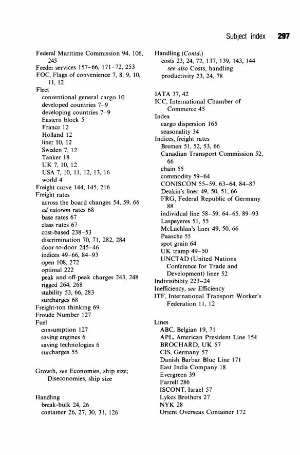
Federal Maritime Commission 94 106 245 ' ,
Feeder services 157-66, 171-72,253 FOC, Flags of convenience 7, 8, 9, 10,
11, 12 Fleet
conventional general cargo 10 developed countries 7-9 developing countries 7-9 Eastern block 5 France 12 Holland 12 liner to, 12 Sweden 7, 12 Tanker 18 UK 7,10,12 USA 7,10, 11, 12, 13, 16 world 4
Freight curve 144, 145, 216 Freight rates
across the board changes 54, 59, 66 ad valorem rates 68 base rates 67 class rates 67 cost-based 238-53 discrimination 70, 71, 282, 284 door-to-door 245-46 indices 49-66, 84-93 open 108, 272 optimal 222 peak and off-peak charges 243, 248 rigged 264, 268 stability 53, 66, 283 surcharges 68
Freight-ton thinking 69 Froude Number 127 Fuel
consumption 127 saving engines 6 saving technologies 6 surcharges 55
Growth, see Economies, ship size; Diseconomies, ship size
Handling break-bulk 24, 26 container 26, 27, 30, 31, 126
Subject index 297
Handling (Contd.) costs 23, 24, 72, 137, 139, 143, 144
see also Costs, handling productivity 23, 24, 78
lATA 37,42 ICC, International Chamber of
Commerce 45 Index
cargo dispersion 165 seasonality 34
Indices, freight rates Bremen 51, 52, 53, 66 Canadian Transport Commission 52
66 '
chain 55 commodity 59-64 CONISCON 55-59, 63-64, 84-87 Deakin's liner 49, 50, 51, 66 FRG, Federal Republic of Germany
88 individual line 58-59, 64-65, 89-93 Laspeyeres 51, 55 McLachlan's liner 49, 50, 66 Paasche 55 spot grain 64 UK tramp 49-50 UNCTAD (United Nations
Conference for Trade and Development) liner 52
Indivisibility 223-24 Inefficiency, see Efficiency ITF, International Transport Worker's
Federation 11, 12
Lines ABC, Belgian 19, 71 APL, American President Line 154 BROCHARD, UK 57 CIS, Germany 57 Danish Barbar Blue Line 171 East India Company 18 Evergreen 39 Farrell 286 ISCONT, Israel 57 Lykes Brothers 27 NYK 28 Orient Overseas Container 172
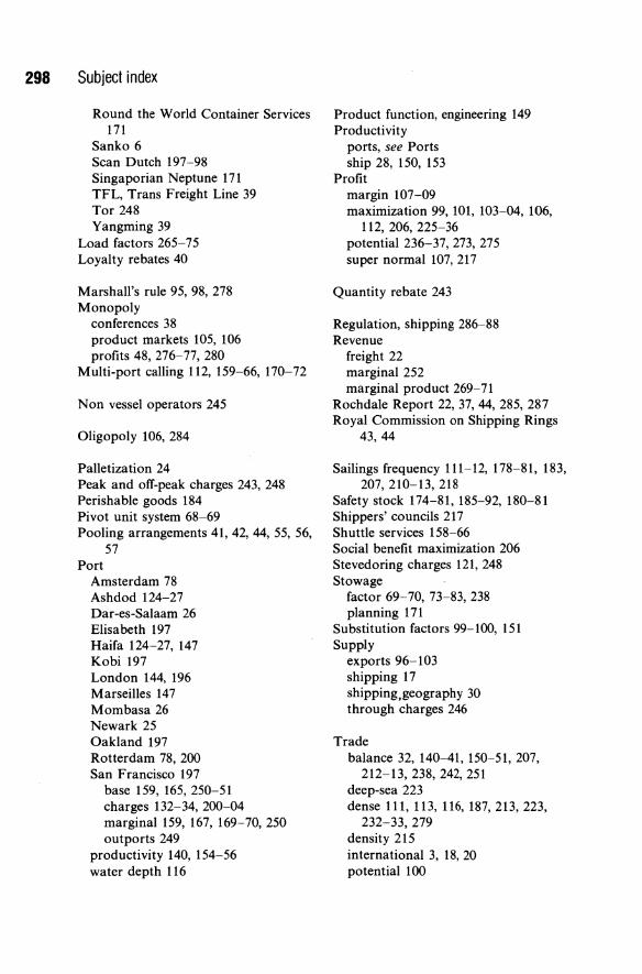
298 Subject index
Round the World Container Services 171
Sanko 6 Scan Dutch 197-98 Singaporian Neptune 171 TFL, Trans Freight Line 39 Tor 248 Yangming 39
Load factors 265-75 Loyalty rebates 40
Marshall's rule 95, 98, 278 Monopoly
conferences 38 product markets 105, 106 profits 48, 276-77, 280
Multi-port calling 112, 159-66, 170-72
Non vessel operators 245
Oligopoly 106, 284
Palletization 24 Peak and ofT-peak charges 243, 248 Perishable goods 184 Pivot unit system 68-69 Pooling arrangements 41, 42, 44, 55, 56,
57 Port
Amsterdam 78 Ashdod 124-27 Dar-es-Salaam 26 Elisabeth 197 Haifa 124-27, 147 Kobi 197 London 144, 196 Marseilles 147 Mombasa 26 Newark 25 Oakland 197 Rotterdam 78, 200 San Francisco 197
base 159, 165, 250-51 charges 132-34,200-04 marginal 159, 167, 169-70,250 outports 249
productivity 140, 154-56 water depth 116
Product function, engineering 149 Productivity
ports, see Ports ship 28, 150, 153
Profit margin 107-09 maximization 99, 101, 103-04, 106,
112, 206, 225-36 potential 236-37,273, 275 super normal 107, 217
Quantity rebate 243
Regulation, shipping 286-88 Revenue
freight 22 marginal 252 marginal product 269-71
Rochdale Report 22,37,44, 285, 287 Royal Commission on Shipping Rings
43,44
Sailings frequency 111-12, 178-81,183, 207, 210-13, 218
Safety stock 174-81,185-92,180-81 Shippers' councils 217 Shuttle services 158-66 Social benefit maximization 206 Stevedoring charges 121, 248 Stowage
factor 69-70, 73-83, 238 planning 171
Substitution factors 99-100, 151 Supply
exports 96-103 shipping 17 shipping,geography 30 through charges 246
Trade balance 32, 140-41, 150-51,207,
212-13,238,242,251 deep-sea 223 dense Ill, 113, 116, 187, 213, 223,
232-33, 279 density 215 international 3, 18, 20 potential 100

Trade (Contd.) routes
Australia-Europe 19 Far East-Europe 4 FRG, Federal Republic of Germany-Israel 54 France-Morocco 73, 78 Israel 73, 274 Italy-North Atlantic 54 Japan-US 154 Mediterranean 239 South East Asia 73 USA 4, 19,40,215,239,274-75
short-sea 222 Tramp market 273, 277, 281 Transit storage 195
Subject index 299
UNCTAD, United Nations Conference for Trade and Development 7, 11, 38, 45-46, 52, 78, 133
shipping code 46-47, 287 Unit value of commodity 73-83, 96, 98,
109 USA
exports and imports 108 major trade routes 265-67 shipping act, 1984 38, 44, 47-48, 245,
285,288 see also Anti-trust law
Value of service pricing 70, 72
Wilson square route formula 182