linear, discrete, dynamic-systems analysis: the z...
TRANSCRIPT

CHAPTER 2
Linear, Discrete, Dynamic-Systems Analysis: The z-Transform
2.1 INTRODUCTION
The unique element in the structure of Fig. 1.1 is the die;ital computer. The fundamental character of the digital computer is that it takes a finite time to compute answers, and it does so with only finite precisioll. The purpose of this chapter is to develop tools of analysis necessary to understand and to guide the design of programs for a computer acting as a linear, dynamic control component. Needless to say, digital computers can do many things other than control linear, dynamic systems; it is our purpose in this chapter to examine their characteristics when doing this elementary control task and to develop the basic analysis tools needed to write programs for a real-time control computer.
2.2 LINEAR DIFFERENCE EQUATIONS
We assume that the analog-to-digital converter (A/D) in Fig. 1.1 takes samples of" the signal y at discrete times and passes them to the computer so that y(kT) = y(kT). The job of the computer is to take these sample values and compute in some fashion the signals to be put out through the digital-to-analog converter (D I A). The characteristics of the AID and D / A converters will be discussed later. Here we consider the treatment of the data inside the computer. Suppose we call the · input signals up to the kth sample eo, el, e2, . .. , ek, and the output signals prior to that time un, UI, U2, . .. , Uk-I. Then, to get the next output, we have the machine com-
13
14 CHAPTER 2 SYSTEMS ANALYSIS
pute some function, which we can express in symbolic form as
(2.1)
Because we plan to emphasize the elementary and the dynamic possibilities, we assume that the function f in (2.1) is linear and depends on only a finite number of past e's and u's. Thus we write
Uk = -alUk-l-a2Uk-2-" ·-anuk-n+boek+blek-l + .. ·+bmek-mo (2.2)
Equation (2.2) is called a linear recurrence equation or difference equation and, as we shall see, has many similarities with a linear differential equation. The name "difference equation" derives from the fact that we could write (2.2) using Uk plus the differences in Uk, which are defined as
VUk = Uk - Uk-l
V2
Uk = VUk - VUk-l
vnUk = Vn-1Uk - Vn-1Uk_l
(first difference),
(second difference),
(nth difference). (2 .3)
If we solve (2.3) for the values of Uk, Uk-I, and Uk-2 in terms of differences, we find
Uk = Uk;,
Uk-l = Uk - VUk;,
Uk-2 = Uk - 2VUk + V2Uk'
Thus, for a second-order equation with coefficients aI, a2, and bo (we let bl = b2 = 0 for simplicity), we find the equivalent difference equation to be
Although the two forms are equivalent, the recurrence form of (2.2) is more convenient for computer implementation; we will drop the form using differences. We will continue, however, to refer to our equations as "difference equations." If the a's and b's in (2.2) are constant, then the computer is solving a constant-coefficient difference equation (CCDE). We plan to demonstrate later that with such equations the computer can control linear constant dynamic systems and approximate most of the other tasks of linear, constant, dynamic systems, including performing the functions of electronic filters. To do so, it is necessary first to examine methods of obtaining solutions to (2.2) and to study the general properties of these solutions.

2.2 LINEAR DIFFERENCE EQUATIONS 15
35
30
25
20
u(k)
15 -b
10 ,I
5 -
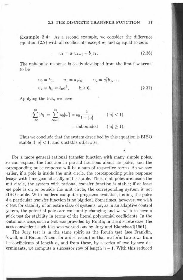
0 0 2 3 4 5 6 7 8
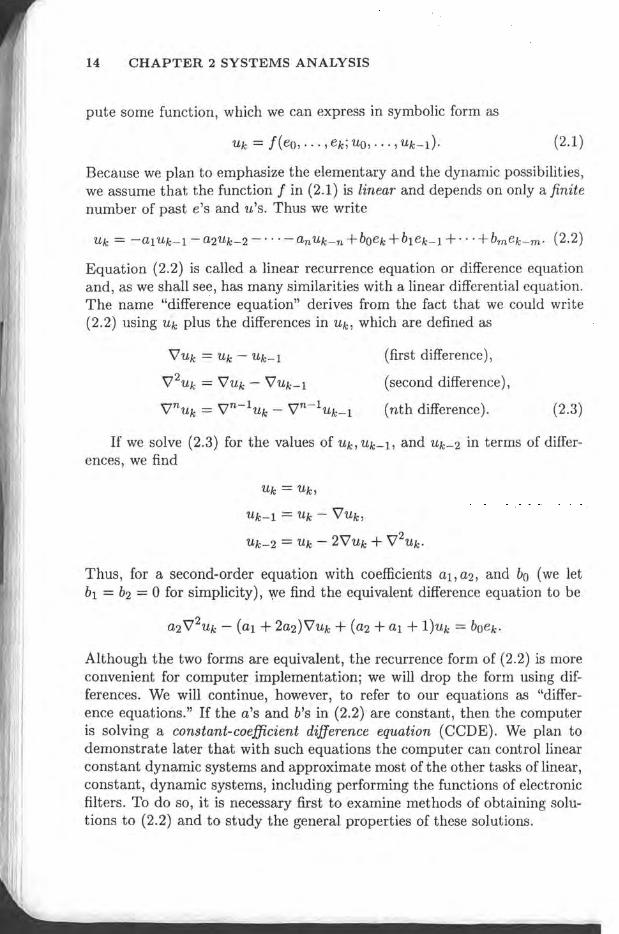
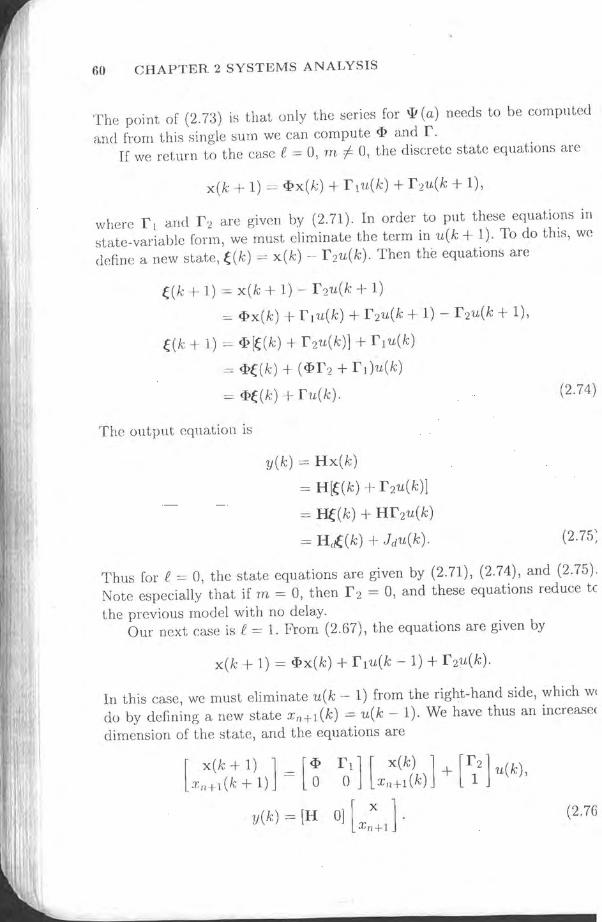
Figure 2.1 The Fibonacci numbers.
To solve a specific CeDE is an elementary matter. We 'need a starting time (k-value) and some initial conditions to characterize the contents of the computer memory at this time. For example, suppose we take the case
(2.4)
and start at k = 2. Here there are no input values, and to compute U2 we need to know the (initial) values for Uo and Ul. Let us take them to be Uo = Ul = 1. The first nine values are 1, 1,2,3,5,8,13,21,34 .... A plot of the values of Uk versus k is shown in Fig. 2.1.
The results, the Fibonacci numbers, are named after the thirteenthcentury mathematicianl who studied them. For example, (2.4) has been used to model the growth of rabbits in a protected environment.2 However that may be, the output of the system represented by (2.4) would seem to be
1 Leonardo Fibonacci of Pisa, who introduced Arabic notation to the Latin world about 1200 A.D. 2Wilde (1964). Assume that Uk represents pairs of rabbits ap.d that babies are born in pairs. Assume that no rabbits die and that a new pair begin reproduction after one period. Thus at time k, we have all the old rabbits, Uk-l, plus the newborn pairs born to the mature rabbits, which are Uk-2.

16 CHAPTER 2 SYSTEMS ANALYSIS
growing, to say the least. If the response of a dynamic system to any finite initial conditions can grow without bound, we call the system unstable. We would like to be able to examine equations like (2.2) and, without having to solve them explicitly, see if they are stable or unstable and even understand the general shape of the solution.
One approach to solving this problem is to assume a form for the solution with unknown constants and to solve for the constants to match the given initial conditions. For continuous, ordinary, differential equations that are constant and linear, exponential solutions of the form est are used. In the case of linear, constant, difference equations, it turns out that solutions of the form zk will do where z has the role of sand k is the discrete independent variable replacing time, t. Consider (2.4). If we assume that u(k) = Azk, we get the equation
Now if we assume z # 0 and A # 0, we can divide by A and multiply by z-k, with the result
or
Z2 = z + 1.
This polynomial of second degree has two solutions, z = 1/2 ± J5/2. Let's call these Zl and Z2. Since our equation is linear, a sum of the individual solutions will also be a solution. Thus, we have found that a solution to (2.4) is of the form
We can solve for the unknown constants by requiring that this general solution satisfy the specific initial conditions given. If we substitute k = 0 and k = 1, we obtain the simultaneous equations
1 = Al + A 2 ,
1 = AlZl + A2Z2.
2.2 LINEAR DIFFERENCE EQUATIONS 17
These equations are easily solved3 to give
A _!+v'5 1 - 2v'5 '
v'5 -1 A2 =-- ·
2v'5
And now we have the complete solution of (2.4) in a closed form. Furthermore, we can see that since Zl = (1 + v'5)/2 is greater than 1, the term in Zl k wiil grow without bound as k grows, which confirms our suspicion that the equation represents an unstable system. We can generalize this result. The equation in Z that we obtain after we substitute u = zk is a polynomial in z known as the characteristic equation of the difference equation. If any solution of this equation is outside the unit circle (has a magnitude greater than one), the corresponding difference equation is unstable in the speCific sense that for some finite initial conditions the solution will grow without bound as time goes to infinity. If all the roots of the characteristic equation are inside the unit circle, the corresponding difference equation is stable.
Example 2.1: Is the equation
u(k) = 0.9u(k - 1) - 0.2u(k - 2)
stable? The characteristic equation is
Z2 - 0.9z + 0.2 = 0,
and the characteristic roots are z = 0.5 and z = 0.4. Since both these roots are inside the unit circle, the equation is stable.
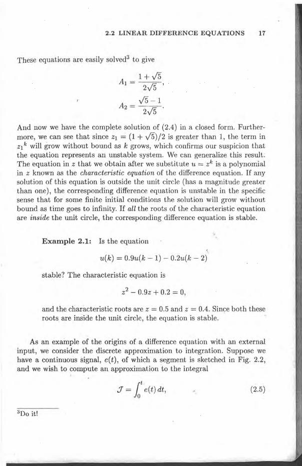
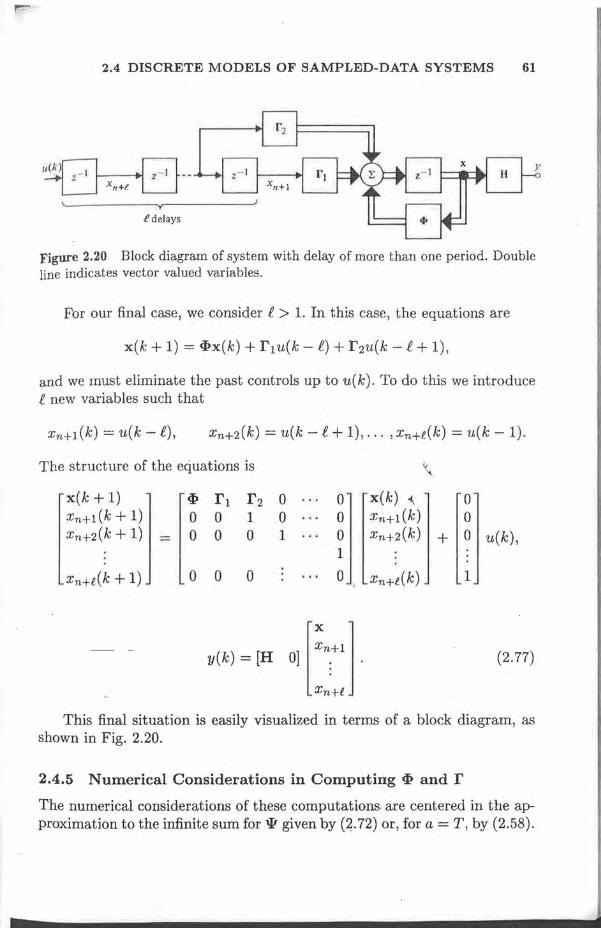
As an example of the origins of a difference equation with an external input, we consider the discrete approximation to integration. Suppose we have a continuous signal, e(t), of which a segment is sketched in Fig. 2.2, and we wish to compute an approximation to the integral
.J = lot e(t) dt, (2.5)
18 CHAPTER 2 SYSTEMS ANALYSIS
e e e
k -- 1 k k-l k k - 1 k
Figure 2.2 Plot of a function and alternative approximations to the area under the curve over a single time interval.
using only the discrete values e(O), ... , e(tk-d, e(tk)' We assume that we have an approximation for the integral from zero to the time tk-I and we call it Uk-I. The problem is to obtain Uk from this information. Taking the view of the integral as the area under the curve e(t), we see that this problem reduces to finding an approximation to the area under the curve between tk-l and tk' Three alternatives are sketched in Fig. 2.2. We can use the rectangle of height ek-I, or the rectangle of height ek, or the trapezoid formed by connecting ek-I to ek by a straight line. If we take the third choice, the area of the trapezoid is
(2.6)
Finally, if we assume that the sampling period, tk - tk-I, is a constant, T, we are led to a simple formula for discrete (trapezoid rule) integration:
(2.7)
If e(t) = t, then ek = kT and substitution of Uk = (T2/2)k2 satisfies (2.7) and is exactly the integral of e. [It should be, because if e( t) is a straight line, the trapezoid is the exact area. J If we approximate the area under the curve by the rectangle of height ek-I, the result is called the Forward Rectangular Rule and is described by
A third possibility is the Backward Rectangular Rule, given by
2.3 THE DISCRETE TRANSFER FUNCTION 19
Each of these integration rules is a special case of our general difference equation (2.2). We will examine the properties of these rules later, in Chapter 4, while discussing means to obtain a difference equation that will be equivalent to a given differential equation.
Thus we see that difference equations can be evaluated directly by a digital computer and that they can represent models of physical processes and approximations to integration. It turns out that if the difference equations are linear with coefficients that are constant, we can describe the relation between u and e by a transfer function, and thereby gain a great aid to analysis and also to the design of linear, constant, discrete controls.
2.3 THE DISCRETE TRANSFER FUNCTION
We will obtain the transfer function of linear, constant, discrete systems by the method of z-transform analysis. A logical alternative viewpoint that requires a bit more mathematics but has some appeal is given in Section 2.7.2. The results are the same. We also show how these same results can be expressed in the state space form in Section 2.3.3.
2.3.1 The z-Transform , '.
If a signal has discrete values eo, el,"" ek, ... we define the z-transform of the signal as the function4 ,5
TO < Izl < Ra, (2.8)
4We use the notation ~ to mean "is defined as." 5In (2.8) the lower limit is -00 so that values of ek on both sides of k = 0 are included. The transform so defined is sometimes called the two-sided z-transform to distinguish it from the one-sided definition, which would be L:;;'" ekz-k. For signals that are zero for k < 0, the transforms obviously give identical results. To take the one-sided transform of Uk-I, however, we must handle the value of U-l,
and thus are initial conditions introduced by the one-sided transform. Examination of this property and other features of the one-sided transform are invited by the problems. We select the two-sided transform because we need to consider signals that extend into negative time when we study random signals in Chapter 8.
20 CHAPTER 2 SYSTEMS ANALYSIS
and we assume we can find values of TO and ilD as bounds on the magnitude of the complex variable z for which the series (2.8) converges. A discussion of convergence is deferred until Section 2.7.
Example 2.2: As an example to illustrate (2.8), consider that the data ek are taken as samples from the time signal e-at l(t) at sampling period T where l(t) is the unit step function, zero for negative t, and one for positive t. Then ek = e-akT l(kT). The z-transform of this is
00 00
L ek z - k = L e-akT z-k
k=-oo 0
e-aT < Izl < 00
z - e-aT
We will return to the analysis of signals and development of a table of useful z-transforms in Section 2.5; we first examine the use of the transform to reduce difference equations to algebraic equations and techniques for representing these as block diagrams.
2.3.2 The Transfer Function
The z-transform has the same role in discrete systems that the Laplace transform has in analysis of continuous systems. For example, the z-transforms for ek and Uk in the difference equation (2.2) or in the trapezoid integration (2.7) are related in a simple way that permits the rapid solution of linear, constant, difference equations of this kind. To find the relation, we proceed by direct substitution. We take the definition given by (2.8) and, in the same way, we define the z-transform of the sequence '{Uk} as
00
U(z) ~ L Uk Z -k
, (2.9) k=-oo
2.3 THE DISCRETE TRANSFER FUNCTION 21
Now we multiply (2.7) by z-k and sum over k. We get
From (2.9), we recognize the left-hand side as U(z). In the first term on the right, we let k - 1 = j to obtain
00 00
L L UjZ-(j+l) = z-lU(z). (2.11) k=-oo j=-oo
By similar operations on the third and fourth terms we can reduce (2.10) to
T U(z) = z-lU(z) + 2[E(z) + z-l E(z)J. (2.12)
Equation (2.12) is now simply an algebraic equation in z and the functions U and E. Solving it we obtain
U(z) = T 1 + z-l E(z). 2 1 - z-l
(2.13)
We define the ratio of the transform of the output to th~ transform of the input as the transfer function, H(z). Thus, in this case, the transfer function for trapezoid-rule integration is
U(z) ~ H(z) = T z + 1. E(z) 2 z - 1
(2.14)
For the more general relation given by (2.2), it is readily verified by the same techniques that
H(z) = bo + b1z- 1 + ... + bmz-m
1 + alz-1 + a2z-2 + ... + anz-n '
and if n 2: m, we can write this as a ratio of polynomials in z as
H(z) = bozn. + blZn-
1 + ... + bm z71-
m
Zfl + al zn - 1 + azzn - 2 + ... "I- an
b(z) - a(z)' (2.15)

22 CHAPTER 2 SYSTEMS ANALYSIS
E(z) U(z) = z- 1 E(z)
Figure 2.3 The unit delay.
The general input-output relation between transforms with linear, constant, difference equations is
U(z) = H(z)E(z). (2.16)
Although we have developed the transfer function with the z-transform, it is also true that the transfer function is the ratio of the output to the input when both vary as zk.
Because H(z) is a rational function of a complex variable, we use the terminology of that subject. Suppose we call the numerator polynomial b(z) and the denominator a( z). The places in z where b( z) = 0 are zeros of the transfer function, and the places in z where a(z) = 0 are the poles of H(z). If Zo is a pole and (z - zo)P H(z) has neither pole nor zero at zo, we say that H(z) has a pole of order p at zoo If p = 1, the pole is simple. The transfer function (2.14) has a simple pole at z = 1 and a simple zero at z = -1.
We can now give a physical meaning to the variable z. Suppose we let all coefficients in (2 .15) be zero except bl and we take bl to be 1. Then H(z) = z-l. But H(z) represents the transform of (2.2), and with these coefficient values the difference equation reduces to
(2.17)
The present value of the output, Uk, equals the input delayed by one period. Thus we see that a transfer function of z-l is a delay of one time unit. We can picture the situation as in Fig. 2.3, where both time and transform relations are shown.
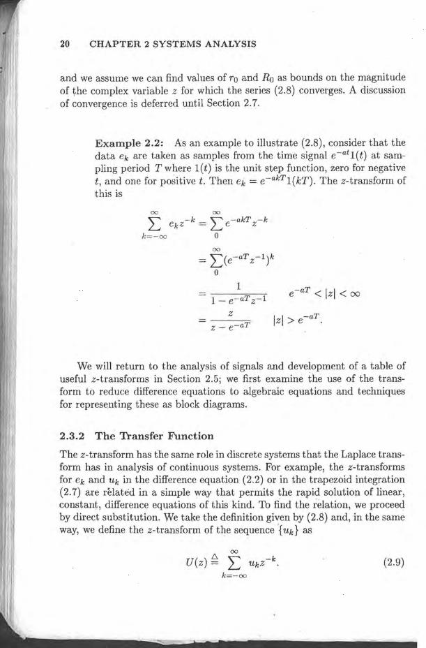
Since the relations of (2.7), (2.14), and (2.15) are all composed of delays, they can be expressed in terms of z- l! Consider (2.7). In Fig. 2.4 we illustrate the difference equation (2.7) using the transfer function z-l as the symbol for a unit delay.
We can follow the operations of the discrete integrator by tracing the signals through Fig. 2.4. For example, the present value of ek is passed to the first summer, where it is added to the previous value ek-l, and the sum is multiplied by T /2 to compute the area of the trapezoid between ek-l and ek. This is the signal marked ak in Fig. 2.4. After this, there is another sum, where the previous output, Uk-I, is added to the new area to form the next
2.3 THE DISCRETE TRANSFER FUNCTION 23
'. I
Figure 2.4 A block diagram of trapezoid integration as represented by (2.7).
value of the integral estimate, Uk. The discrete integration occurs in the loop with one delay, z-l, and unity gain.
2.3.3 Block Diagrams and State-Variable Descriptions
Because (2.16) is a linear algebraic relationship, a system of such relations is described by a system of linear equations. These can be solved by the methods of linear algebra or by the graphical methods of block diagrams. To use block-diagram analysis to manipulate these discrete-transfer-function relationships, there are only four primitive cases: '.( '. 1. The transfer function of paths in parallel is the sum qf the single-path
transfer functions (Fig. 2.5).
2. The transfer function of paths in series is the product of the path transfer functions (Fig. 2.6).
3. The transfer function of a single loop of paths is the transfer function of the forward path divided by one minus the loop transfer function (Fig. 2.7).
4. The transfer function of an arbitrary multipath diagram is given by combinations of these cases. Mason's rule6 can also be used.
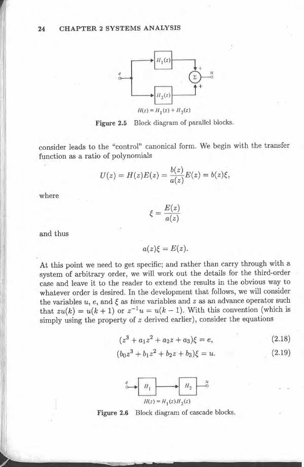
For the general difference equation of (2.2), we already have the transfer function in (2.15). It is interesting to connect this case with a block diagram using only simple delay forms for z in order to see several "canonical" block diagrams and to introduce the description of discrete systems using equations of state.
There are many ways to reduce the difference equation (2.2) to a block diagram involving z only as the delay operator, Z-l. The first one we will
6Mason (1956). See Franklin, Powell, and Emami-Naeini(1986) for a discussion.
24 CHAPTER 2 SYSTEMS ANALYSIS
~ r~ L &--J+
H(z) = HI (z) + H 2(z)
Figure 2.5 Block diagram of parallel blocks.
consider leads to the "control" canonical form. We begin with the transfer function as a ratio of polynomials
where
and thus
b(z) U(z) = H(z)E(z) = a(z) E(z) = b(z)~,
~ = E(z) a(z)
a(z)~ = E(z).
At this point we need to get specific; and rather than carry through with a system of arbitrary order, we will work out the details for the third-order case and leave it to the reader to extend the results in the obvious way to whatever order is desired. In the development that follows, we will consider the variables u, e, and ~ as time variables and z as an advance operator such that zu(k) = u(k + 1) or z-lu = u(k - 1). With this convention (which is simply using the property of z derived earlier), consider the equations
(Z3 + alz2 + a2Z + a3)~ = e,
(boz3 + b1z2 + b2z + b3)~ = U.
~@----+& H(z) = HI (z)H2(z)
Figure 2.6 Block diagram of cascade blocks .
(2.18)
(2.19)
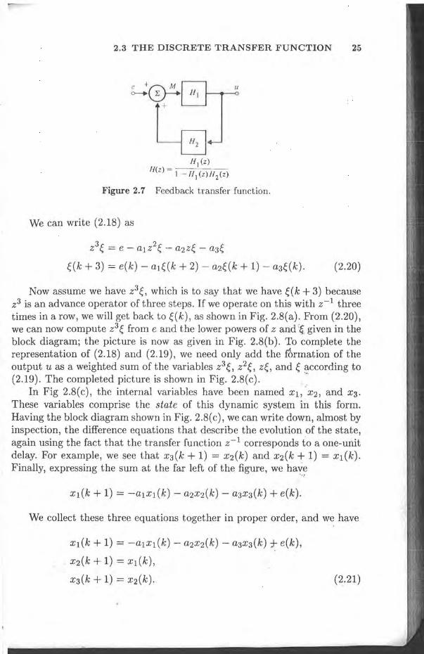
2.3 THE DISCRETE TRANSFER FUNCTION 25
u
HJ (z)
H(z) = \-HJ(z)H
2(z)
Figure 2.1 Feedback transfer function.
We can write (2.18) as
Z3~ = e - alz2~ - a2z~ - a3~
~(k + 3) = e(k) - al~(k + 2) - a2~(k + 1) - a3~(k). (2.20)
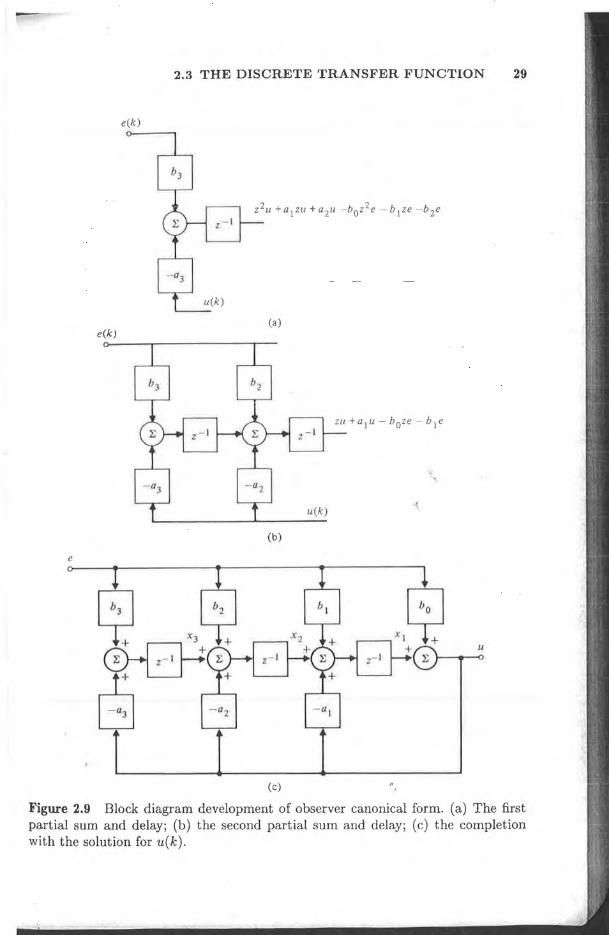
Now assume we have z3~, which is to say that we have ~(k + 3) because z3 is an advance operator of three steps. If we operate on this with z-l three times in a row, we will get back to ~(k), as shown in Fig. 2.8(a). From (2.20), we can now compute z3 ~ from e and the lower powers of z and '~ given in the block diagram; the picture is now as given in Fig. 2.8(b). To complete the representation of (2.18) and (2.19), we need only add the f6rmation of the output u as a weighted sum of the variables z3 ~, z2 ~, z~, and ~ according to (2 .19). The completed picture is shown in Fig. 2.8(c). ".
In Fig 2.8(c), the internal variables have been named Xl, x2, and X3.
These variables comprise the state of this dynamic system in this form. Having the block diagram shown in Fig. 2.8(c), we can write down, almost by inspection, the difference equations that describe the evolution of the state, again using the fact that the transfer function z-l corresponds to a one-unit delay. For example, we see that x3(k + 1) = x2(k) and x2(k + 1) = xI(k). Finally, expressing the sum at the far left of the figure, we have
"f
We collect these three equations together in proper order, and we have
xl(k + 1) = -alxl(k) - a2x2(k) - a3x3(k)::I- e(k),
x2(k + 1) = xl(k),
x3(k + 1) = x2(k). (2.21)

26 CHAPTER 2 SYSTEMS ANALYSIS
W + 3) We)
(a)
Hk + I ) Hk) z" 1
e +
(el
Figure 2.8 Block diagram development of control canonical form. (a) Solving for ~(k); (b) solving for ~(k + 3) from e(k) and past ~\s; (c) solving for U(k) from ~'s.
2.3 THE DISCRETE TRANSFER FUNCTION 27
Using vector-matrix notation,? we can write this in the compact form
where
TJ (2.22a)
and
(2.22b)
The output equation is also immediate except that we must watch to catch all paths by which the state variables combine in the. output. The problem is caused by the bo term. If bo = 0, then u = bl x.1 + b2X2 + b3X3, and the corresponding matrix form is immediate. However, if boo is not 0, Xl
for example not only reaches the output through bl but also by the parallel path with gain -boal. The complete equation is
In vector/matrix notation, we have
where
Cc = [b l - albo b2 - a2bo b3 - a3bo] ,
Dc = [bolo
(2.23a)
(2.23b)
7We assume the reader has some knowledge of matrices. The ;esults we require and references to study material are given in Appendix C. To distinguish vectors and matrices from scalar variables, we will use bold-face type.

28 CHAPTER 2 SYSTEMS ANALYSIS
We can combine the equations for the state evolution and the output to give the very useful and most compact equations for the dynamic system,
x(k + 1) = Aex(k) + B ee(k),
u(k) = Cex(k) + Dee(k), (2.24)
where Ae and B e for this control canonical form arc given by (2.22), and C e and D c are given by (2.23).
The other canonical form we want to illustrate is called the observer canonical form and is found by starting with the difference equations in operator / transform form as
In this equation, the external input is e(k), and the response is u(k), which is the solution of this equation. The terms with factors of z are time-shifted toward the future with respect to k and must be eliminated in some way. To do this, we assume at the start that we have the u( k), and of course the e(k) , and we rewrite the equation as
Here, every term on the right is multiplied by at least one power of z, and thus we can operate on the lot by z-l as shown in the partial block diagram drawn in Fig. 2.9(a).
Now in this internal result there appear a2u and -b2 e, which can be cancelled by adding proper multiples of u and e, as shown in Fig. 2.9(b), and once they have been removed, the remainder can again be operated on by z-l.
If we continue this process of subtracting out the terms at k and operating on the rest by z-l, we finally arrive at the place where all that is left is u alone! But that is just what we assumed we had in the first place, so connecting this term back to the start finishes the block diagram, which is drawn in Fig. 2.9(c).
A preferred choice of numbering for the state components is also shown in the figure. Following the technique used for the control form, we find that the matrix equations are given by
x(k + 1) = Aox(k) + Boe(k),
u(k) = Cox(k) + Doe(k), (2.25)
2.3 THE DISCRETE TRANSFER FUNCTION 29
e(k)
e(k)
e
(c)
Figure 2.9 Block diagram development of observer canonical form. (a) The first partial sum and delay; (b) the second partial sum and delay; (c) the completion with the solution for u(k).

30 CHAPTER 2 SYSTEMS ANALYSIS
where
e(k) z + 1 z2 _ z
,2 _ 0.5, + 0.25
z2_ 1.6z+0.81
u(k)
Figure 2.10 Block diagram of a cascade realization.
[ -a, 1
~] , Ao= -a2 0 -a3 0
[b' - bOa,] Bo= b2 - bOa2 ,
b3 - bOa3
Co = [1 0 0]'
Do = [bol·
The block diagrams of Figs. 2.8 and 2.9 are called direct canonical realizations of the transfer function H(z) because the gains of the ralizations are coefficients in the transfer-function polynomials. Another Ilseful form is obtained if we realize a transfer function by pJacing sev ral fu· t- 01' se ondorder direct forms in series with each other, a cascade canonical form. In this case, the H(z) is represented as a product of fa ·tors, an th pol sand zeros of the transfer function are clearly represented in the coefficients.
For example, suppose we have a transfer function
H(z) = z3 + 0.5z2 - 0.25z + 0.25 z4 - 2.6z3 + 2.4z2 - 0.8z
(z + 1)(z2 - 0.5z + 0.25) = (z2 - z)(z2 - 1.6z + 0.8)'
The zero factor z + 1 can be associated with the pole factor z2 - Z to form one second-order syst,em, and the zero factor z2 - 0.5z + 0.25 can be associated with the second-order pole factor z2-1.6z+0.8 to form another. The cascade factors, which could be realized in a direct form such as control or' observer form, make a cascade form as shown in Fig. 2.10.
2.3.4 Relation of Transfer Function to Pulse Response
We have shown that a transfer function of z-l is a unit delay in the time domain. We can also give a time-domain meaning to an arbitrary transfer func-
2.3 THE DISCRETE TRANSFER FUNCTION 31
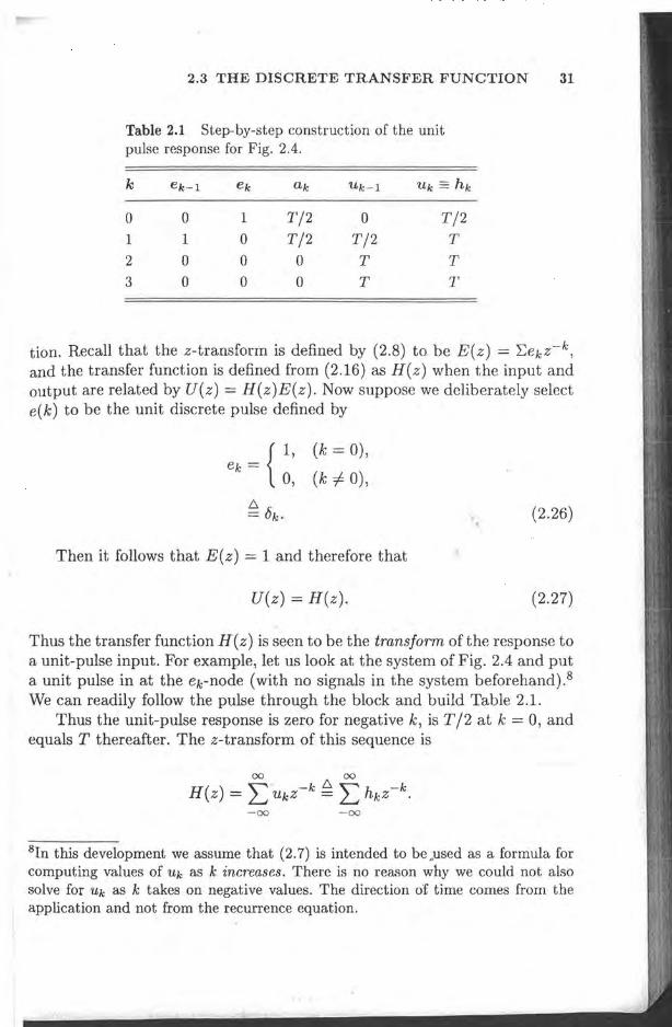
Table 2.1 Step-by-step construction of the unit pulse response for Fig. 2.4.
k Ck-l Ck ak Uk-l Uk == hk
0 0 1 T/2 0 T/2 1 1 0 T/2 T/2 T 2 0 0 0 T T 3 0 0 0 T T
tion. Recall that the z-transform is defined by (2.8) to be E(z) = "L-ekz-k, and the transfer function is defined from (2 .16) as H(z) when the input and output are related by U(z) = H(z)E(z). Now suppose we deliberately select e(k) to be the unit discrete pulse defined by
{I,
ek = 0,
(k = 0),
(k i= 0),
Then it follows that E(z) = 1 and therefore that
U(z) = H(z).
(2.26)
(2.27)
Thus the transfer function H(z) is seen to be the transform ofthe response to a unit-pulse input. For example, let us look at the system of Fig. 2.4 and put a unit pulse in at the ek-node (with no signals in the system beforehand).8 We can readily follow the pulse through the block and build Table 2.1.
Thus the unit-pulse response is zero for negative k, is T /2 at k = 0, and equals T thereafter. The z-transform of this sequence is
00 00
H(z) = L Uk Z -k ~ L hk Z -
k. -00 -00
8In this development we assume that (2.7) is intended to be pused as a formula for computing values of Uk as k increases. There is no reason why we could not also solve for Uk as k takes on negative values. The direction of time comes from the application and not from the recurrence equation.
32 CHAPTER 2 SYSTEMS ANALYSIS
eo + el z - 1
ho + h1 z - 1
eO hO+ el hoz - 1
+ eOh1z- 1 +e2hoz - 2
+e1 h 1z- 2
+ eoh2z-2
+e3hOz - 3
+ e2hl z - 3
+ e1h2z - 3
+eOh3z - 3
+ .. . + .. .
Figure 2.11 Representation of the product E(z}H(z} as a product of polynomials.
If we add T /2 to the zO-term and subtract T /2 from the whole series, we have a simpler sum, as follows:
00 T H( z ) = LTz-k --
k=O 2
T T (1 < Izl) - 1 - z-l 2
2T - T(l- z-l) - 2(1- z-l)
T+Tz- 1
- 2(1- z-l)
Tz+1 2z-1
(1 < Izl). (2.28) = - - -
Of course, this is the transfer function we obtained in (2.13) from direct analysis of the difference equation.
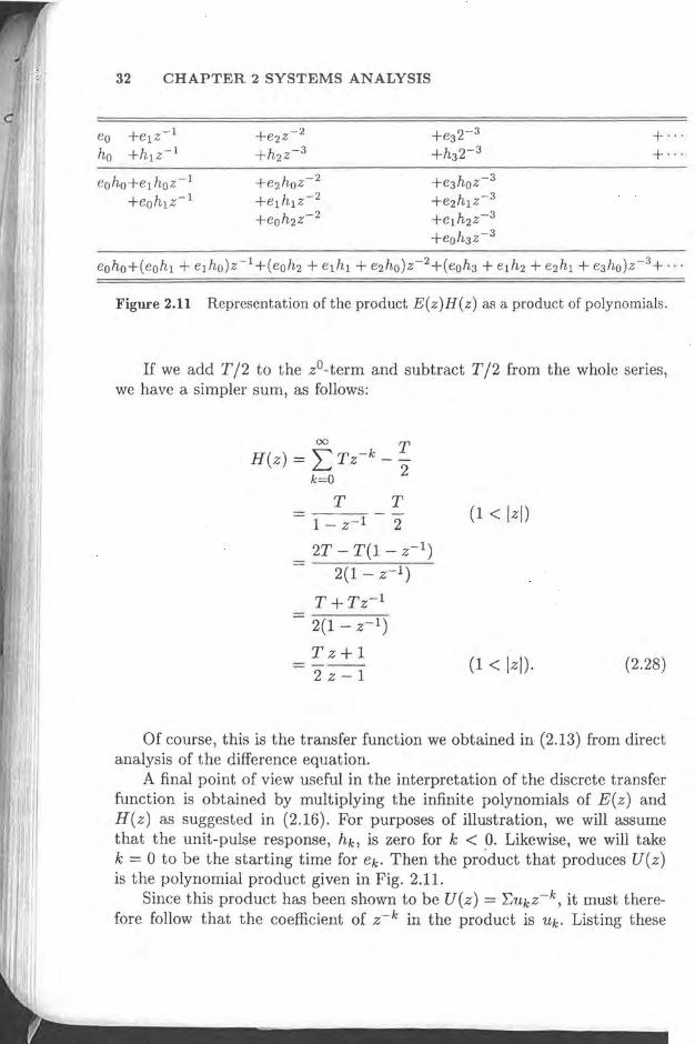
A final point of view useful in the interpretation of the discrete transfer function is obtained by multiplying the infinite polynomials of E(z) and H( z ) as suggested in (2.16). For purposes of illustration, we will assume that the unit-pulse response, hk, is zero for k < O. Likewise, we will take k = 0 to be the starting time for ek. Then the product that produces U(z) is the polynomial product given in Fig. 2.11.
Since this product has been shown to be U(z) = L,Uk Z-k, it must therefore follow that the coefficient of z-k in the product is Uk . Listing these

2.3 THE DISCRETE TRANSFER FUNCTION 33
coefficients, we have the relations
Uo = eoho,
Ul = eOhl + e1ho,
u2 = eOh2 + e1h1 + e2hO,
u3 = eoh3 + e1h2 + e2hl + e3hO'
The extrapolation of this simple pattern gives the result
k
Uk = L ejhk-j· j=O
By exten~ion, we let the lower limit of the sum be -00 and the upper limit be +00:
00
Uk = L ejhk_ j . j=-oo
(2.29)
Negative values of j in the sum correspond to inputs appli~d before time equals zero. Values for j greater than k occur if the unit-pulse response is nonzero for negative arguments. By definition, such a s¥stem, which responds before the input that causes it occurs, is called noncausal. This is the discrete convolution sum and is the analog of the convolution integral that relates input and impulse response to output in linear, constant, continuous systems.
To verify (2.29) we can take the z-transform of both sides:
00 00 00
L Uk Z -k = L z-k L ejhk _ j .
k=-oo k=-oo j=-oo
Interchanging the sum on j with the sum on k leads to
00 00
U(z) = L ej L Z-khk_j'
j=.,.-oo k=-oo
Now let k ~ j = l in the secoIld sum:
00 00
U(z) = L ej L h1z-(l+j),
j=-oo 1=-00
34 CHAPTER 2 SYSTEMS ANALYSIS
but z-(l+j) = z-l [j which leads to , 00 00
U(z) = 2: ejz- j 2: hlZ-l,
j=-OO 1=-00
and we recognize these two separate sums as
U(z) = E(z)H(z).
We can also derive the convolution sum from the properties of linearity and stationarity. First we need more formal definitions of "linear" and
"stationary. " 1. Linearity: A system with input e and output U is linear if superposition
applies, which is to say, if ul(k) is the response to el(k) and u2(k) is the response to e2 (k ), then the system is linear if and only if, for every
scalar a and (3, the response to ael + (3e2 is aUl + (3u2' 2. Stationarity: A system is stationary, or time invariant, if a time shift in
the input results in only a time shift in the output. For example, if we !;ak the system at r st (no internal energy in the system) and apply a certain signal (k), suppose we observe a response u(k). If we repeat this experiment aL any later time when the system is again at rest and we apply Lh sbifted input, e(k - N), if we see u(k - N), then the system
is stationary. .
These properties can be used to derive the convolution in (2.29) as follows. If response to a unit pulse at k = 0 is h(k), then response to a pulse of intensity eo is eoh( k) if the system is linear. Furthermore, if the system is constant, then a delay of the input will delay the response. Thus, if
e = {e l'
0,
k = l,
k =1= l,
then the response will be elhk-l· Finally, by linearity again, the total response at time k to a sequence of
these pulses is the sum of the responses, namely,
or k
Uk = 2: e/hk-I· 1=0
2.3 THE DISCRETE TRANSFER FUNCTION 35
Now note that if the input sequence began in the distant past, we must include terms for l < 0, perhaps back to l = -00. Similarly, if the system should be noncausal, future values of e where l > k may also come in. The general case is thus (again)
00
Uk = L e/hk-/. 1=-00
2.3.5 External Stability and Jury's Test
(2.30)
A very important qualitative property of a dynamic system is stability, and we can consider internal or external stability. Internal stability is concerned with the responses at all the internal variables such as those that appear at the delay elements in a canonical block diagram as in Fig. 2.8 or Fig. 2.9 (the state). Otherwise we can be satisfied to consider only the external stability as given by the study of the input-output relation described for the linear stationary case by the convolution (2.30). These differ in that some internal modes might not be connected to both the input and the output of a given system.
For external stability, the most common definition of appropriate response is that for every Bounded Input, we should have a Bounded Output. If this is true we say the system is BIBO stable. A test for BIBO stability can be given directly in terms of the unit-pulse response, hk .1<'irst we consider a sufficient condition. Suppose the input ek is bounded, that is, there is an M such that
led::; M < 00 for alIi. (2.31)
If we consider the magnitude of the response given by (2.30), it is easy to see that
which is surely less than the sum of the magnitudes as given by
-00
But, because we assume (2.31), this result is in turn bounded by "
00
(2.32) -00
36 CHAPTER 2 SYSTEMS ANALYSIS
Thus the output will be bounded for every bounded input if
00
L I hk- ti < 00 . (2 .33)
l==-oo
This condition is also necessary, for if we consider the bounded (by I!) input
h-l el=--
Ih_ll
=0
and apply it to (2.30), the output at k = 0 is
00
uo = L elh-l l=-oo
(2.34)
Thus, unless the condition given by (2.34) is true, the system is not BIBO stable.
Example 2.3: The test given by (2.34) can be applied to the unit pulse response used to compute (2.13) and given as the uk-column
in Table 2.1 on page 31:
ho = T/2,
hk =T, k > 0, 00
L Ihkl = T/2 + LT = unbounded. 1
(2.35)
Thus this discrete approximation to integration is not (BIBO) stable!
2.3 THE DISCRETE TRANSFER FUNCTION 37
Example 2.4: As a second example, we consider the difference equation (2.2) with all coefficients except al and bo equal to zero:
(2.36)
The unit-pulse response is easily developed from the first few terms to be
Uo = bo ,
k ~ o. (2.37)
Applying the test, we have
(Ial < 1)
= unbounded (Ial ~ 1).
Thus we conclude that the system described by this equation is BIBO stable if lal < 1, and unstable otherwise. '(,
(,
For a more general rational transfer function with many simple poles, Ne can expand the function in partial fractions about its poles, and the :orresponding pulse response will be a sum of respective terms. As we saw )arlier, if a pole is inside the unit circle, the corresponding pulse response iecays with time geometrically and is stable. Thus, if all poles are inside the mit circle, the system with rational transfer function is stable; if at least me pole is on or outside the unit circle, the corresponding system is not 3IBO stable. With modern computer programs available, finding the poles )f a particular transfer function is no big deal. Sometimes, however, we wish o test for stability of an entire class of systems; or, as in an adaptive control ,ystem, the potential poles are constantly changing and we wish to have a luick test for stability in terms of the literal polynomial coefficients. In the :ontinuous case, such a test was provided by Routh; in the discrete case, the nost convenient such test was worked out by Jury and Blanchard(1961).
The Jury test is in the same spirit as the Routh t~st (see Franklin, lowell, and Emami-Naeini for a discussion) in that we for'm two rows from he coefficients of length n, and from these, by a series of two-by-two deerminants, we compute a successor row of length n:- 1. With this reduced
38 CHAPTER 2 SYSTEMS ANALYSIS
length row we form another successor of length n - 2 and so on until we have a row of length 1. The test consists of examining the sign of the first entries in selected rows. As with the Routh test, the Jury test is much more difficult to derive than to use; here we illustrate only the use.
If we have a transfer function H(z) = b(z)ja(z), then this system will be stable if and only if all roots of a(z) = aozn + aiZn- i + ... + an are inside the unit circle. To test for this condition by the Jury test, multiply a( z) by -1 if necessary to make the sign of ao positive. Then form rows of the coefficients, the even rows being in reversed order, as follows:
ao ai an an an-i ao bo bi
bn-i bn-2
The entries in the third row are formed from the second-order determinants using the first column of the first two rows with each of the other columns from these rows starting from the right and dividing by ao· The result can be expressed by the formulas:
an bo = ao - -an,
ao an
bi = ai - -an-i, ao an
bk = ak - -an-k, ao
The elements in the third row are reversed to form the fourth row and the process is repeated. For example, the elements of the fifth row are given by
The original polynomial is stable' ( has all roots inside the unit circle) if all the terms in the first columns of the odd rows are positive, that is, if
ao > O,bo > O,eo > 0, .... This test is readily implemented in a computer program.9
9See STABLE in Table E.1 in Appendix E.

-2.3 THE DISCRETE TRANSFER FUNCTION 39
Example 2.5: To illustrate the use of Jury's test, we consider first the simple second-order polynomial
a(z) = z2 + alz + a2.
Thp. Jury array is
1
(1 - a~)2 - ar(l - a2)2
1 - a§
al a2
al 1 al - ala2
1 - a§
From row three, we have the condition that 1 - a22 > 0, and from this we conclude that
-1 < a2 < 1.
From row five, we can factor out (1 - a2)2 to conclude that
and thus, <.
and
From these inequalities, we can draw the stability triangle shown in Fig 2.12.
- I
Figure 2.12 Stability triangle for the general, real, second-order polynomial.
40 CHAPTER 2 SYSTEMS ANALYSIS
Example 2.6: For the next example, consider the polynomial
a(z) = Z3 - 2.1z2 + 1.6z - 0.4.
The Jury array is
1 -0.4 0.84 0.76
0.1524 -0.139 0.0256
-2.1 1.6
-1.46 -1.46 -0.139 0.1524
1.6 -2.1 0.76 0.84
-0.4 1
The test is from the odd rows: 1 > 0,0.84 > 0,0.1524 > 0, 0.0256 > 0, and we conclude that a system with this polynomial as its denominator would be stable. As a matter of fact, the poles are at z = 0.5 and z = 0.8 ± O.4j.
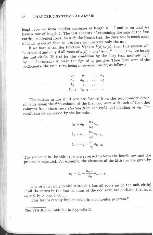
Example 2.7: As a third example, consider the polynomial
Z3 - 2.6z2 + 2.4z - 0.8
The odd rows only of the Jury array are
1 0.36
0.0756 o
-2.6 2.4 -0.68 0.32
-0.0756
-0.8
From these computations we conclude that the polynomial doe~ not have all its roots inside the unit circle; and, because the last term is zero and a small perturbation would send it either way, inside OJ
outside, there must be at least one root exactly on the unit circle, In fact, the roots are z = 1 and z = 0.8 ± O.4j.
As an aid to testing stability, it can be shown that it is necessary for ( stable polynomial (with positive first term) that the polynomial evaluatec
2.4 DISCRETE MODELS OF SAMPLED-DATA SYSTEMS 41
at z = 1 and z = -1 must both be positive. The first value is just the sum of the coefficients, and the second is the sum with alternating sign changes. These two tests are quickly done and can save time if the only purpose is to be sure that the system is stable; many unstable systems will be rejected by these simple tests without going through the entire Jury array. In the previous case, for instance, the sum of coefficients is .zero and we need go no further; the polynomial cannot be stable.
2.4 DISCRETE MODELS OF SAMPLED-DATA
SYSTEMS
The systems and signals we have studied thus far have been defined in discrete time only. Most of the dynamic systems to be controlled, however, are continuous systems and, if linear, are described by continuous transfer functions in the Laplace variable s. The interface between the continuous and discrete domains are the AID and the D I A converters as shown in Fig. 1.1. In this section we develop the analysis needed to compute the discrete transfer function between the samples that come from the digital computer ,to the D I A converter and the samples that are picked up by the AID converter.1° The situation is drawn in Fig. 2.13. <.
2.4.1 Using the z-Transform
We wish to find the discrete transfer function from the input samples u(kT) (which probably come from a computer of some kind) to the output samples, y(kT) picked up by the AID converter. Although it is possibly confusing at first, w follow c;onventi n and call the discrete transfer function G (z) when th ontinuous transfer fun ·tion is G(s). Although G(z) and G(s) are entirely differ nt functions , t,hey do describe the same plant, and the use of s for the continuous transform and z for the discrete transform is always maintained. To find G(z) we need only observe that the y(kT) are samples of the plant output when the input is from the D I A converter. As for the D I A converter, we assume that this device, commonly called a zero-order hold or ZOH, accepts a sample u(kT) at t = kT and holds its output constant
lOIn Chapter 3, a comprehensive frequency analysis of sa;npled data systems is presented. Here we undertake only the special problem of 'finding the sample-tosample discrete transfer function of a continuous system between a D I A and an A/D.

42 CHAPTER 2 SYSTEMS ANALYSIS
y(kT)
Figure 2.13 The prototype sampled-data system.
at this value until the next sample is sent at t = kT + T. The piecewisl constant output of the D / A is the signal, u( t), that is applied to the plant
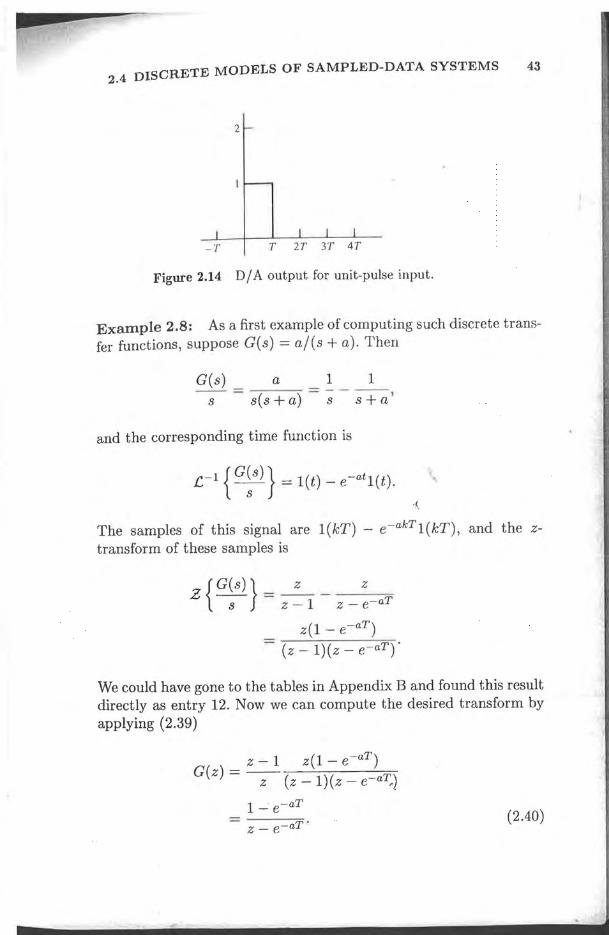
Our problem is now really quite simple because we have just seen tha the discrete transfer function is the z-transform of the samples of the outpu when the input samples are the unit pulse at k = O. If u(kT) = 1 for k = I and u(kT) = 0 for k f. 0, the output of the D 1 A converter is a pulse of widtl T seconds and height 1, as sketched in Fig. 2.14. Mathematically, this puIs· is given by l(t) - l(t - T). Let us call the particular output in response tl the pulse shown in Fig. 2.14 Yl (t). This response is the difference betweeJ the step response [to l(t) ] and the delayed step response [to l(t - T)]. Th Laplace transform of the step response is G (s) 1 s. Thus in the transforr domain the unit pulse response of the plant is
(2.38
and the required transfer function is the z-transform of the samples of th inverse of Y1 (s), which can be expressed as
G(z) = Z{Yl(kT)}
= Z{.c-1{y1(s)}} ~ Z{Yl(S)}
= Z {(I _ e-Ts ) G~S)} .
This is the sum of two parts . The first is Z {G (s) / s }, and the second is
Z{ e-T8 G(s)1 s} = z-l Z{ G(s)1 s}
because e-Ts is exactly a delay of one period. Thus the transfer function
G(z) = (1 _ z-l)Z {G~s)} (2.3!
2.4 DISCRETE MODELS OF SAMPLED-DATA SYSTEMS 43
2
-T T 2T 3T 4T
Figure 2.14 D / A output for unit-pulse input.
Example 2.8: As a first example of computing such discrete transfer functions, suppose G(s) = a/(s + a). Then
G(s) a - s- - s(s + a) = -; - -s +- a '
1 1
and the corresponding time function is
£-1 {G;s)} = l(t) _ e-at l(t).
The samples of this signal are l(kT) - e-akT l(kT), and the ztransform of these samples is
z{G(s)} __ Z _ Z
s - Z - 1 Z - e-aT
z(1 - e-aT )
(z - 1)(z - e- aT )'
We could have gone to the tables in Appendix B and found this result directly as entry 12. Now we can compute the desired transform by applying (2.39)
z - 1 z(1 - e-aT ) G(z) = -- -,-~--,---,---~=
z (z - 1)(z - e-aT~)
1 ~ e-aT
z - e-aT ' (2.40)

44 CHAPTER 2 SYSTEMS ANALYSIS
Example 2.9: We consider the double integrator characteristic of a single mass, such as the satellite, for which the transfer function is G(8) = 1/82. We have
G(z) = (1- z-l)Z {s~ }
This time we refer to the tables in Appendix B and find that the transform of 1/83 is
and therefore
T2 z(z + 1) 2 (z -1)3'
(2.41)
For more complex systems than those in Examples 2.8 and 2.9, use of a CAD package is recommended.l1
2.4.2 Continuous Time Delay
We now c'(msider computing the discrete transfer function of a continuous system with pure time delay. The responses of many chemical processcontrol plants exhibit pure time delay because there is a finite time of transport of fluids or materials between the process and the controls and/or the sensors. Also, we must often consider finite computation time in the digital controller, and this is exactly the same as if the process had a pure time delay. With the techniques we have developed here, it is possible to obtain the discrete transfer function of such processes exactly, as Example 2.10 illustrates.
Example 2.10: We consider the example suggested by the fluid mixer problem described in Appendix A.3, for which
G(s) = e-'\8 H(s).
llSee X-C2D in Table E.l.
1 l

2.4 DISCRETE MODELS OF SAMPLED-DATA SYSTEMS 45
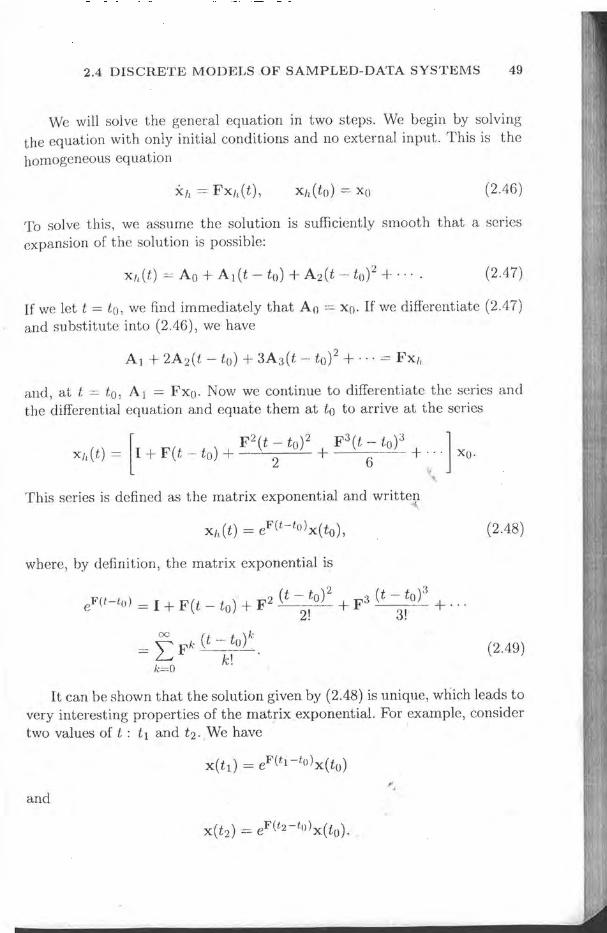
The term e- ),. · re] resents th delay ~f A se n~~. whi ·1I indud s b h tb pr eSB delay and Lbe, 'on~put~tlOn r~elay, if any. 'V'! assuI~e that H(.') is a rational transfer [unct! n, 10 pr~par L~lS functlOn [or cornputati n of the z-transforrn, We -first de·fin' an Integer e and a po 'itivc llurnb ·r m l e~s than 1.0 su h that), = iT - mI' . With thes definitions we can wnte
G(s) _fTsemTsH(s) --=e .
s s
Because C is an integer, this term reduces to z- e when we take the ztransform. Because m < 1, the transform of the other term is quite direct. We select H(s) = a/(s + a) and, after the partial fraction expansion of H (s ) / s, we have
G(z)=-Z ---z - 1 { emTs
emTs
} zP+l S S + a
To complete the transfer function, we need the z-transforms of the inverses of the terms in the braces. The first term is a unit step shifted left by mT seconds, and the second term is an. exponential shifted left by the same amount. Because m < 1, these shifts are less than one full period, and no sample is picked up in~negative time. The signals are sketched in Fig. 2.15.
The samples are given by l(kT) and c aT(k+m)l(kT). The corresponding z-transforms are z/(z - 1) and ze- amT /(z - e-aT ). Consequently the final transfer function is
z - 1 1 {z ze-amT
} G(z) = -z- zP z - 1 - z - e-aT
= z - 1 { Z[Z - e- uT - (z - l)e- (i,mTl} zP .. (z - l)(z - e-nT)
( -amT) Z + 0: = 1 - e n( _ T)' z" z - e a
where the zero position is at - 0: = - (e- amT - e-aT ) / (1 - e-amT ). Notice that this zero is near the origin of the z-p(~tne when m is near 1 and moves outside the unit circle to near - 00 .when m approaches O. For the specific values of the mixer, we take a = 1, T = 1, and
46 CHAPTER 2 SYSTEMS ANALYSIS
2 r-
l I I I I I I I
-2T -T 0 T 2T 3T 4T 5T 6T
2
- 2T -T 0 T 2T 3T 4T 5T 6T
Figure 2.15 Sketch of the shifted signals showing sample points .
). = 1.5. Then we can compute that f = 2 and m = 0.5. For these values, we get
G(z) = z + 0.6065 . z2(z - 0.3679)
2.4.3 State-Space Form
(2.42)
Computing the z-transform using the Laplace transform as in (2.39) is a very tedious business that is unnecessary with the availability of computers. We will next develop a formula using state descriptions that will remove most of the calculations to the computer, where it is better done. A continuous, linear, constant-coefficient system of differential equations can always be expressed as a set of first-order matrix differential equations:
(2.43)
where u is the control input to the system and w is a disturbance input. The output can be expressed as a linear combination of the state, x, and the input as
y = Hx+Ju. (2.44)

2.4 DISCRETE MODELS OF SAMPLED-DATA SYSTEMS 47
u e
Figure 2.16 Satellite attitude control in classical representation.
Often the sampled-data system being described is the plant of a control problem, and the parameter J in (2.44) is zero and will frequently be omitted.
Example 2.11: Application of state representation to the equations of the satellite attitude-control example shown in Fig. 2.16 and described in Appendix A yields
[ ;~] = [~ ~] [~~] + [~] u, ~ ~
F G
e = y = [1 0] [Xl] , '-v-' X2
H \(
"-
(2.45)
which, in this case, turns out to be a rather involved way of writing -<.
The representations (2.43) and (2.44) are not unique. Given one state representation, any nonsingular linear transformation of that state such as { = Tx is also an allowable alternative realization of the same system.
If we let { = Tx in (2.43) and (2.44), we find
t = Ti = T(Fx + Gu + Glw)
= TFx + TGu + TGIW,
t = TFT-I{ + TGu + TGlw,
y = HT-'l{ + Ju.
If we designate the system matrices for the new state { as A, B, C, andD, then '
t = A{+ Bu+ BIW, y =.C{+ Du,

48 CHAPTER 2 SYSTEMS ANALYSIS
where
u~ u(t) I I y(t) ~T) Df A .. F, G, H ~ AID
Figure 2.17 System definition with sampling operations shown.
C = HT- I D = J. ,
Example 2.12: As an illustration, we can let ~l = X2 and ~2 = Xl
in (2.45); or, in matrix notation, the transformation to interchange the states is
T=[~ ~]. In this case T- 1 = T, and application of the transformation equations to the system matrices of (2.45) gives
A = [~ ~] C = [0 1J .
Most often, a change of state is made to bring the description matrices into a useful canonical form. We saw earlier how a single high-order difference equation could be represented by a state description in control or in observer canonical form. Also, there is a very useful state description corresponding to the partial-fraction expansion of a transfer function. State transformations can take a general description for either a continuous or a discrete system and, subject to some technical restrictions, convert it into a description in one or the other of these forms, as needed.
We wish to use the state description to establish a general method for obtaining the difference equations that represent the behavior of the continuous plant. Fig. 2.17 again depicts the portion of our system under consideration. Ultimately, the digital controller will take the samples y(k), operate on that sequence by means of a difference equation, and put out a sequence of numbers, u(k), which are the inputs to the plant. The loop will, therefore, be closed. To analyze the result, we must be able to relate the samples of the output y(k) to the samples of the control u(k). To do this, we must solve (2.43).
2.4 DISCRETE MODELS OF SAMPLED-DATA SYSTEMS 49
We will solve the general equation in two steps. We begin by solving the equation with only initial conditions and no external input. This is the homogeneous equation
)cit = Fxdt), (2.46)
To solve this, we assume the solution is sufficiently smooth that a series expansion of the solution is possible:
(2.47)
If we let t = to, we find immediately that Ao = Xo. If we differentiate (2.47) and substitute into (2.46), we have
and, at t = to, Al = Fxo. Now we continue to differentiate the series and the differential equation and equate them at to to arrive at the series
This series is defined as the matrix exponential and writtel). .. (2.48)
where, by definition, the matrix exponential is
(t - t )2 (t - t )3 eF(t-to) = 1+ F(t _ to) + F2 0 + F3 0 + ...
2! 3!
= ~ Fk (t - to)k ~ k' (2.49) 1.:=0 .
It can be shown that the solution given by (2.48) is unique, which leads to very interesting properties of the matrix exponential. For example, consider two values of t : tl and t2' We have
". and
50 CHAPTER 2 SYSTEMS ANALYSIS
Because to is arbitrary also, we can express X(t2) as if the equation solution began at h, for which
Substituting for x(td gives
We now have two separate expressions for x( t2 ), and, if the solution IS
unique, these must be the same. Hence we conclude that
(2.50)
for all t2, tl, to. Note especially that if t2 = to, then
Thus we can obtain the inverse of eFt by merely changing the sign of t! We will use this result in computing the particular solution to (2.43).
The particular solution when u is not zero is obtained by using the method of variation of parameters. 12 We guess the solution to be in the form
xp(t) = eF(t-tolv(t), (2.51)
where v(t) is a vector of variable parameters to be determined [as contrasted to the constant parameters x(to) in (2.48)]. Substituting (2.51) into (2.43), we obtain
FeF(t-tol v + eF(t-tol v = FeF(t-tol v + Gu,
and, using the fact that the inverse is found by changing the sign of the exponent, we can solve for v as
v(t) = e-F(t-tolGu(t).
12Due to Joseph Louis Lagrange, French mathematician (1736-1813). We assume w = 0, but because the equations are linear, the effect of w can be added later.
2.4 DISCRETE MODELS OF SAMPLED-DATA SYSTEMS 51
Assuming that the control u(t) is zero for t < to, we can integrate v from to to t to obtain
Hence, from (2.51), we get
and simplifying, using the results of (2.50), we obtain the particular solution ( convolution)
(2.52)
The total solution for w = 0 and u i- 0 is the sum of (2.48) and (2.52):
x(t) = eF(t-to)x(to) + rt eF(t-T)Gu(r)dr. ~ lto
~
(2.53)
We wish to use this solution over one sample period to obtain a difference equation: hence we juggle the notation a bit (let t = kT + T and to equal kT) and arrive at a particular version of (2.53):
ikT+T
x(kT + T) = eFT x(kT) + eF(kT+T-T)Gu(r)dr. kT
(2.54)
This result is not dependent on the type of hold because u is specified in terms of its continuous time history, u(t), over the sample interval. A common and typically valid assumption is that of a zero-order hold (ZOH) with no delay, that is,
u(r) = u(kT), kT ::; r < kT + T.
If some other hold is implemented or if there is a delay between the application of the control from the ZOH and the sample po'int, this fact can be accounted for in the evaluation of the integral in (2.54) The equations for a delayed ZOH will be given in the next subsection. To facilitate the solution
52 CHAPTER 2 SYSTEMS ANALYSIS
of (2.54) for a ZOH with no delay, we change variables in the integral from
T to 'T/ such that
Then we have
If we define
'T/ = kT+T-T.
cI> = eFT,
r = loT eFT) d'T/G,
(2.55)
(2.56a)
(2.56b)
Eqs. (2.55) and (2.44) reduce to difference equations in standard form:
x(k + 1) = cI>x(k) + ru(k) + r1w(k),
y(k) = Hx(k), (2.57)
where we include the effect of an impulsive or piecewise constant disturbance, w, and assume that J = 0 in this case. If w is a constant, then rl is given by (2.56b) with G replaced by Gl. If w is an impulse, then rl = Gl.13 The cI> series expansion
can also be written
cI> = 1+ FTq" (2.58)
where
13If w(t) is not a function of only its sample values, then an integral like that of (2.54) is required to describe its influence on x(k + 1). Random disturbancE:ls are treated in Chapt~r 9.
2.4 DISCRETE MODELS OF SAMPLED-DATA SYSTEMS 53
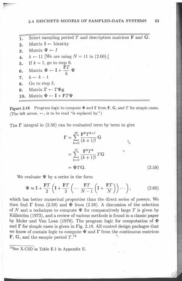
1. Select sampling period T and description matrices F and G. 2. Matrix 1 f- Identity
3. Matrix W f- I 4 . k f- 11 [We are using N = 11 in (2.60).]
5. If k = 1, go to step 9. FT
6. Matrix W f- 1 + k W 7. k f- k-1 8. Go to step 5. 9. Matrix r f- TWg
10. Matrix «l> f- 1 + FTw
Figure 2.18 Program logic to compute c}) and r from F, G, and T for simple cases. (The left arrow, ;-, is to be read "is replaced by.")
The r integral in (2.56) can be evaluated term by term to give
00 FkTk+1 r=2: G
k=O (k + I)!
00 FkTk =2: TG
k=O (k + I)!
=wTG.
We evaluate W by a series in the form
W ~ 1 + FT (I + FT ( ... ~ (I + FT)) ... ) , . 2 3 N-1 N
(2.59)
(2.60)
which has better numerical properties than the direct series of powers. We then find r from (2.59) and «l> from (2.58). A discussion of the selection of N and a technique to compute W for comparatively large T is given by Kallstrom (1973), and a review of various methods is found in a classic paper by Moler and Van Loan (1978). The program logic for computation of «l> and r for simple cases is given in Fig. 2.18. All control design packages that we know of contain logic to compute «l> and r from the continuous matrices F, G, and the sample period T .14 ,.,
14See X-C2D in Table E.1 in Appendix E.
54 CHAPTER 2 SYSTEMS ANALYSIS
To compare this method of representing the plant with the discrete transfer functions, we can take the z-transform of (2.57) with w = 0 and obtain
therefore
[zI - <1>]X(z) = rU( z),
Y(z) = HX(z);
Y(z) = H[zI _ <I>r1r. U(z)
(2.61a)
(2.61b)
(2.62)
Example 2.13: For the satellite attitude-control example, the <1>
and r matrices are easy to calculate using (2.58) and (2.59) and the values for F and G defined in (2.45) . Since F2 = 0 in this case, we have
= [ ~ ~ ] +[ ~ ~] T = [ ~ ~ ] ,
r = [IT+F~; +F:nG = { [~ ~ ] + [ ~ ~] ~2 W] = [T;e ]·
hence, using (2.61), we obtain
~~:~ = [1 0] {z [~ ~] _ [~ ~]} -1 [Ti2] _ T2 (z + 1) - ""2 (z -1)2'
which is the same result that would be obtained using (2.39) and the z-transform tables. .
Note that to compute Y/U we find that the denominator is the determinant det(zI - <1», which comes from the matrix inverse in (2.62) . This
2.4 DISCRETE MODELS OF SAMPLED-DATA SYSTEMS 55
determinant is the characteristic polynomial of the transfer function, and the zeros of the determinant are the poles of the plant. We have two poles at z = 1 in this case, corresponding to the two integrations in this plant's equations of motion.
We can explore further the question of poles and zeros and the statespace description by considering again the transform equations (2.61). An interpretation of transfer-function poles from the perspective of the corresponding difference equation is that a pole is a value of z such that the equation has a nontrivial solution when the forcing input is zero. From (2.61a), this implies that the linear eigenvalue equations
[zI - <I>JX(z) = [OJ
have a nontrivial solution. From matrix algebra the well-known requirement for this is that det(zI - <I» = O. In the present case, we have
det[zI - <I>J = det [[~ ~] - [~ ~]]
= det [ z ~ 1 z ~ 1 ]
= (z _1)2 = 0,
.,
which is the characteristic equation, as we have seen. To compute the poles numerically when the matrices are given, one would use an eigenvalue routine. I5
Along the same line of reasoning, a system zero is a value of z such that the system output is zero even with a nonzero state-and-input combination. Thus if we are able to find a nontrivial solution for X(zo) and U(zo) such that Y(zo) is zero, then Zo is a zero of the system. Combining the two parts of (2.57), we must sati~fy the requirement
[ZI
H- <I> -r] [X(z)] = [OJ
. 0 U(z) . (2.63)
Once more the condition for the existence of nontrivial solutions is that the determinant of the square coefficient system matriJ5 be zero. I6 For the
15See EIGENV in Table E.l. 16We do not consider here the case of different numbers of inputs and outputs.

56 CHAPTER 2 SYSTEMS ANALYSIS
satellite example, we have
[
z - 1
det ~ -T
z -1 o
-T2/2 ] -T o
[ - T
= 1 . det z _ 1
~+T2+cn(Zl) T2 T2
=+2 z +2 T2
= + 2 (z + 1).
Thus we have a single zero at z = -1, as we have seen from the transfer function. Again, to compute the values of the zeros, called transmission zeros, good algorithms exist in matrix algebra.
17
2.4.4 State-Space Models for Systems with Delay
Thus far we have discussed the calculation of discrete state models from continuous, ordinary differential equations of motion. Now we present the formulas for including a time delay in the model and also a time prediction up to one period ;which corresponds to the modified z-transform as defined by Jury. We begin with a state-variable model that includes a delay in control
action. The state equations are
x(t) = Fx(t) + Gu(t - >'),
y=Hx.
The general solution to (2.64) is given by (2 .53); it is
If we let to = kT and t = kT + T, then
kT+T x(kT + T) = eFT x(kT) + ~T eF(kT+T-
T) GU(T - >.) dT.
(2.64)
17 See ZEROS in Table E.1. In using this function, one must be careful to account properly for the zeros that are at infinity; the function might return them as very large numbers that the user must remove to uncover the finite zeros.
2.4 DISCRETE MODELS OF SAMPLED-DATA SYSTEMS 57
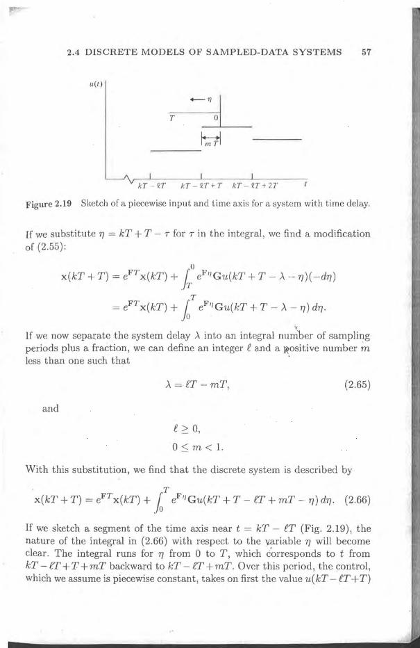
ll(t)
T
kT-2T+T kT-2T+2T
Figure 2.19 Sketch of a piecewise input and time axis for a system with time delay.
If we substitute T/ = kT + T - T for T in the integral, we find a modification of (2.55):
(J
x(kT + T) = eFT x(kT) +.k eF11Gu(kT + T - A - T/)( -dT/)
T = eFT x(kT) + la eF11Gu(kT + T - A - T/) dT/.
'.(
If we now separ:ate the system delay A into an integral number of sampling periods plus a fraction, we can define an integer e and a ~ositive number m less than one such that .
and
A = eT - mT,
e > 0,
O::;m<1.
(2.65)
With this substitution, we find that the discrete system is described by
. T x(kT + T) = eFT x(kT) +.10 eF11Gu(kT + T - P.T + mT - T/) dT/. (2.66)
If we sketch a segment of the time axis near t = kT - P.T (Fig. 2.19), the nature of the integral in (2.66) with respect to the variable T/ will become clear. The integral runs for T/ from 0 to T, which c'arresponds to t from kT - P.T + T + mT backward to kT - P.T + mT. Over this period, the control, which we assume is piecewise constant, takes on first the value u( kT - P.T + T)
58 CHAPTER 2 SYSTEMS ANALYSIS
and then the value u(kT-eT). Therefore, we can break the integral in (2.66)
into two parts as follows:
x(kT + T) == eFT x(kT) + rmT eF77 G dT) u(kT - iT + T) Jo
+ rT eF77G dryu(kT - iT)
JmT == ipx(kT) + rlu(kT - eT) + r2u(kT - iT + T). (2.67)
In (2.67) we defined
rl == rT eF77G dT), and
(2.68)
JmT
To complete our analysis it is necessary to express (2.67) in standard statespace form. To do this we must consider separately the cases of e == 0, e == 1,
For e == 0, A == -mT ac aIding to (2.65), which impli "S not d lay put and i > l. predi tion. Becaus mT is restrict,ed to be less than T, however the outpnt will not show a sampl before k == 0 and the discrete sysLem will b "U a1. The r suit is that the discrete system computed with e == 0, m i 0 will show th . respons> at t == 0, which th · same system with .e == 0 m == 0 would show at t == mT. In other words, by taking £ == 0 and m i 0 w' pi k up th, response values between the normal sampling instants. In z-trans(oT theory, the transform of the syst,em with I. == 1 m 'lOis called th · modifier z_transfo
rm.18 The state-variable form r quires that we valuate the iut 'gral:
in (2.68). To do so we first convert rl to a form similar to tb . integral £0 r2. From (2.68) we factor out tbe onstant matrix G to obtain
rl == rT eF77 dT) G.
JmT
If we set a == ry - mT in this integral, we have
rT- mT rl == Jo eF(mT+u)daG
rT- mT == eFm Jo e
Fu daG.
18See Jury (1964) or Ogata (1987).
(2.6
2.4 DISCRETE MODELS OF SAMPLED-DATA SYSTEMS 59
For notational purposes we will define, for any positive nonzero scalar num
ber, a, the two matrices
'l1(a) :::: - eFu deJ. 1 fa a 0
In terms of these matrices, we have
rl ::::(T - mT)~(mT)'l1(T - mT)G,
r2 ::::mT'l1(mT)G.
(2.70)
(2.71)
The definition (2.70) is also useful from a computational point of view. If we recall the series definition of the matrix exponential,
00 Fkak ~(a) :::: eFa
:::: ~ -,--, k==O k.
then we get
'\.
But now we note that the series for ~(a) can be written as
00 Fk k
~(a) :::: 1+ E k~ .
If we let k :::: j + 1 in the sum, then, as in (2.58), we have
00 Fjai = I+~ aF
;==0 (j + 1)! ".
:::: 1+ alJ1(a)F.
(2.72)
(2.73)
60 CHAPTER 2 SYSTEMS ANALYSIS
The point of (2.73) is that only the series for 'l1 (a) needs to he compnted and from this single sum we can compute <I> and r.
If we return to the case £ = 0, Tn oF 0, the discrete state equations are
where r l and r2 are given by (2.71). In order to put these equations in state-variable form, we must eliminate the term in u(k + 1). To do this, we define a new state, ~(k) = x(k) - r2u(k). Then the equations are
~(k + 1) = x(k + 1) - r2u(k + 1)
= <I>x(k) + rlu(k) + r2u(k + 1) - r2u(k + 1),
~ (k + 1) = <1> [~ ( k) + r 2 u ( k )] + r 1 u ( k )
= <1>( ( k) + (<I> r 2 + r 1 ) U ( k )
= <I>((k) + ru(k) .
The output eqllation is
y(k) = Hx(k)
= H[~(k) + r2u(k)]
= m(k) + H r2U (k)
= Hc/€(k) + hu(k).
(2.74)
Thus for £ = 0, the state equations are given by (2.71), (2.74), and (2.75). Note especially that if m = 0, then r2 = 0, and these equations reduce tc
the previous model with no delay. Our next case is £ = 1. From (2.67), the equations are given by
In this case, we must eliminate u(k - 1) from the right-hand side, which WI
do by defining a new state Xn+l (k) = u(k - 1). We have thus an increa-se< dimension of the state, and the equations are
[ x(lc + 1) 1 [<1> r1l [ x(k) 1 + [r21 u(k),
xn+l(k + 1) - 0 0 x ll+l(k) 1
y(k) = [H 0] [ x 1 Xn+l
(2.76
2.4 DISCRETE MODELS OF SAMPLED-DATA SYSTEMS 61
f--Xn-+-l-+B --
L-________ ~y~--------~
fdelays
Figure 2.20 Block diagram of system with delay of more than one period. Double line indicates vector valued variables.
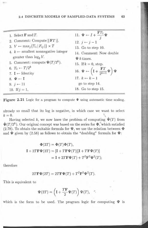
For our final case, we consider f > 1. In this case, the equations are
and we must eliminate the past controls up to u(k). To do this we introduce f new variables such that
Xn+l(k) = u(k - f), xn+2(k) = u(k - f + 1), ... ,xn+e(k) = u(k -1).
The structure of the equations is If
"-
x(k + 1) <I> r1 r2 0 0 x(k) ~ 0 Xn+l (k + 1) 0 0 1 0 0 xn+l(k) 0 xn+2(k + 1) = 0 0 0 1 0 xn+2(k) + 0 u(k),
1
xnH(k + 1) 0 0 0 0 xnH(k) 1
y(k) = [H 0] [:.,+1]. xn+e
(2.77)
This final situation is easily visualized in terms of a block diagram, as shown in Fig. 2.20.
2.4.5 Numerical Considerations in Computing <I> and r The numerical considerations of these computations. are centered in the approximation to the infinite sum for'll given by (2.72) Of, for a = T, by (2.58).
62 CHAPTER 2 SYSTEMS ANALYSIS
The problem is that if FT is large, then (FT)N IN! becomes extremely large before it becomes small, and before acceptable accuracy is realized most computer number repl'esentations will overflow, destroying the value of the computation, KiilIstr"m (1973) has analyzed a technique used by Kalman and Englar (1966), which has b en found effective by Moler and Van Loan (1978). The basi idea comes from (2,50) with t2 - to = 2T and tl - to = T,
namely,
(2.78)
Thus, if T is too large, we can compute the series for T 12 and square the result. If T 12 is too large, we compute the series for T 14, and so on, until we find a k such that T 12k is not too large. We need a test for deciding on the value of k. We propose to approximate the series for 'It, which can be
written
(T) _ N-l[F(TI2k)]1 00 (FTI2k)j _ A
'It k - L ( , , + L . , - 'It + R. 2 j=o J + 1). j=N (J + 1).
We will select k, the factor that decides how much the sample period is divided down, to yield a small remainder term R. Kiillstrom suggests that we estimate the size of R by the size of the first term ignored in ~, namely,
A simpler method is to select k such that the size of FT divided by 2k is less than 1. In this case, the series for FT 12k will surely converge. The rule
is to select k such that n
2k > II FT II = max L I Fij I T. J i=l
Taking the log of both sides, we find
k > 10g2 \I FT \I ,
from which we select
k = max( flog2 \I FT 1\,0), (2.79)
where the symbol r x means the smallest integer greater than x. The maximum of this integer and zero is taken because it is possible that II FT II is
2.4 DISCRETE MODELS OF SAMPLED-DATA SYSTEMS 63
=--1. Select F and T.
2. Comment: Compute // FT II· 3. V ~ maXj{~i / Fij /} x T
4. k ~ smallest nonnegative integer
greater than log2 V.
5. Comment: compute 'l1(T /2 k).
6. Tl ~ T/2 k
7. I ~ Identity
8. 'l1 ~ I
9. j ~ 11
10. Ifj = 1,
11. 'l1 ~ I + F~l 'l1 J
12. j ~ j - 1
13. Go to step 10.
14. Comment: Now double
'l1 k times.
15. If k = 0, stop.
16. 'l1 ~ (I + 2~:1 'l1 ) 'l1
17. k ~ k - 1
go to step 14.
18. Go to step 15.
Figure 2.21 Logic for a program to compute W using automatic time scaling.
already so small that its log is negative, in which case we want to select k = O. ~
Having selected k, we now have the problem of computing ~(T) from 4!(T/2k ). Our original concept was based on the series for cp ;'which satisfied (2.78). To obtain the suitable formula for 'l1, we use the relation between cp and 'l1 given by (2.58) as follows to obtain the "doubling" formula for 'l1:
therefore
cp(2T) = cp(T)cp(T),
1+ 2TF'l1(2T) = [I + TF'l1(T)][1 + TF'l1(T)]
= 1+ 2TF'l1(T) + T2F2'l12(T);
This is equivalent to
.Td')rr\ _ (T I TF .Tdrr\ \ .Trfrr\ X\"'.L) - \..I.'TY\.L}j ~\.L),
which is the form to be used. The program logic for comp'uting 'l1 is

64 CHAPTER 2 SYSTEMS ANALYSIS
shown in Fig. 2.21.19 This algorithm does not include the delay discussed in Section 2.4.4. For that, we must implement the logic shown in Fig. 2.20. 20
2.5 SIGNAL ANALYSIS AND DYNAMIC RESPONSE
In Section 2.3 we demonstrated that if two variables are related by a linear constant difference equation, then the ratio of the z-transform of the output signal to that of the input is a function of the system equation alone, and the ratio is called the transfer function. A method for study of linear constant discrete systems is thereby indicated, consisting of the following steps:
1. Compute the transfer function of the system H (z).
2. Compute the transform of the input signal, E(z).
3. Form the product, E(z)H(z), which is the transform of the output signal, U.
4. Invert the transform to obtain u(kT).
If the system description is available in difference-equation form, and if the input signal is elementary, then the first three steps of this process require very little effort or computation. Th final step, however, is tedious if done by hand, and, because we williat r b pI" ccupied with design f transfer functions to give desirable responses w attach great benefit to gaioing intuition for the kind of response to be exp cted [1' m a transform without actually inverting it. Our approa h to this probl In is to present a r pertoire of elementary signals with known ~ atures and to learn their representation in the transform or z-domain. Thus, when given an unknown transform, we will be able, by reference to these known solutions, to infer the major features of the time-domain signal and thus to determine whether the unknown is of sufficient interest to warrant the effort of detailed time-respons€ computation. To begin this process of attaching a connection between th( time domain and the z-transform domain, we compute the transforms of c few elementary signals.
19See X-C2D in Table E.l 20 See DELAY in Table E.l.