a2 introduction to control theory: discrete time linear

A2 Introduction to Control Theory:Discrete Time Linear Systems

4 lectures Michaelmas Term 2020 Kostas MargellosTutorial sheet 2A2C [email protected]

Syllabus

Discrete time linear systems. The z-transform and its properties. Conversion be-tween difference equations and z-transform transfer functions. Obtaining the dis-crete model of a continuous system plus zero order hold from a continuous (Laplace)transfer function. Mapping from s-plane to z-plane. Significance of pole positionsand implications to stability. Discrete time system specifications. Discrete timestate space systems. Discrete time solutions. Euler discretization.

Lecture notes

These lecture notes are provided as handouts. These notes as well as the lectureslides that follow the same structure are also available on the web (Canvas).

The first four chapters of the notes follow in part lecture material that was producedand was previously taught by Prof. Mark Cannon. His input and his permission touse material from his lecture notes is gratefully acknowledged.

Any comments or corrections shall be sent to [email protected]

2

Recommended text

• G F Franklin, J D Powell & M Workman Digital Control of Dynamic Systems3rd edition, Addison Wesley, 1998.

Other reading

• R C Dorf & R H Bishop Modern Control Systems Pearson Prentice Hall, 2008

• K J Astrom & R M Murray Feedback Systems: An Introduction for Scientistsand Engineers Princeton University Press, 2008

The course follows the first book above which will be referred to as [Franklin etal, 1998]; reference to particular book chapters and sections is provided throughoutthe notes. Consulting the book for detailed elaboration on several concepts as wellas for additional examples and exercises is highly recommended.

3 CONTENTS

Contents

1 Introduction 5

1.1 Digitization . . . . . . . . . . . . . . . . . . . . . . . . . . . . . . 5

1.2 Motivating examples . . . . . . . . . . . . . . . . . . . . . . . . . 6

1.3 Organization of the notes . . . . . . . . . . . . . . . . . . . . . . 8

2 Discrete time linear systems and transfer functions 9

2.1 Sampling and discrete time systems . . . . . . . . . . . . . . . . . 9

2.2 The z-Transform . . . . . . . . . . . . . . . . . . . . . . . . . . . 11

2.3 Properties of the z-transform . . . . . . . . . . . . . . . . . . . . 14

2.4 The discrete transfer function . . . . . . . . . . . . . . . . . . . . 16

2.5 Pulse response and convolution . . . . . . . . . . . . . . . . . . . 18

2.6 Computing the inverse z-transform . . . . . . . . . . . . . . . . . 22

2.7 Summary . . . . . . . . . . . . . . . . . . . . . . . . . . . . . . . 23

3 Discrete models of sampled data systems 24

3.1 Pulse transfer function models . . . . . . . . . . . . . . . . . . . . 24

3.2 ZOH transfer function . . . . . . . . . . . . . . . . . . . . . . . . 28

3.3 Signal analysis and dynamic response . . . . . . . . . . . . . . . . 30

3.4 Laplace and z-transform of commonly encountered signals . . . . . 30

3.5 Summary . . . . . . . . . . . . . . . . . . . . . . . . . . . . . . . 33

4 Step response and pole locations 34

4.1 Poles in the z-plane . . . . . . . . . . . . . . . . . . . . . . . . . 34

4.2 The mapping between s-plane and z-plane . . . . . . . . . . . . . 38

CONTENTS 4

4.3 Damping ratio and natural frequency . . . . . . . . . . . . . . . . 40

4.4 System specifications . . . . . . . . . . . . . . . . . . . . . . . . 40

4.5 Summary . . . . . . . . . . . . . . . . . . . . . . . . . . . . . . . 46

5 Discrete time linear systems in state space form 47

5.1 State space representation . . . . . . . . . . . . . . . . . . . . . . 47

5.2 Solutions to discrete time linear systems . . . . . . . . . . . . . . 50

5.3 Stability of discrete time linear systems . . . . . . . . . . . . . . . 54

5.4 Summary . . . . . . . . . . . . . . . . . . . . . . . . . . . . . . . 58

6 Appendix: The inverse z-transform 60

5 Introduction

1 Introduction

1.1 Digitization?

Discrete time systems are dynamic systems whose inputs and outputs are definedat discrete time instants. Within a control context, digitization is the process ofconverting a continuous controller (Figure 1) into a set of difference equations thatcan be implemented by a computer within a digital control system (Figure 2). Thedigital controller operates on samples of the sensed output, resulting upon analogueto digital (ADC) conversion, rather than the continuous signal y(t). The generateddiscrete time command is then applied to the plant upon digital to analogue (DAC)conversion. This provides practical advantages in terms of accuracy and noiserejection, and simplifies monitoring and simultaneous control of large numbers offeedback loops. However the ability of a digital control system to achieve specifieddesign criteria depends on the choice of digitization method and sample rate.

Figure 1: Continuous controller.

Figure 2: Digital Controller. The dashed box contains sampled signals.

?[Franklin et al, 1998] §3.1

1.2 Motivating examples 6

1.2 Motivating examples

One motivating example involves an autonomous racing platform for miniaturizedcars. For more details regarding this testbed the reader is referred to the set-updeveloped at ETH Zurich (see upper panel of Figure 3), that motivated the recentracing car platform that is now built at University of Oxford (see lower panel ofFigure 3). The platform consists of a race track, an infrared camera based trackingsystem and miniature dnano RC cars. It allows for high-speed, real-time controlalgorithm testing.

Figure 3: Upper panel: RC racing car platform at ETH Zurich (figure taken fromhttp://control.ee.ethz.ch/∼ racing///); Lower panel: RC racing car platform at University ofOxford.

The general architecture underpinning the operation of each car is shown in Figure4. It is based in the following sequence of steps:

1. The camera based vision system captures the cars on the track, each of themcharacterised by a unique marker pattern.

7 Introduction

sensor outputactuation commandreference

control action

Control algorithm

State estimation

Figure 4: Block diagram of control architecture for each racing car.

Figure 5: Embedded board of each car (figure taken from http://control.ee.ethz.ch/∼ racing///).

Figure 6: Left panel: Crazyflie arena; Right panel: On board controller.

2. The position and velocity of each car is estimated by means of some stateestimation algorithm, and is broadcasted to the computer used for controlcalculation.

3. The control inputs (e.g., speed commands) are sent via Bluetooth to the

1.3 Organization of the notes 8

embedded board microcontroller of each car (see Figure 5), which then drivesaround the track.

An additional example involves the CrazyFlies arena, recently developed at theUniversity of Oxford (see Figure 6). The underlying structure and interplay betweenthe continuous dynamics and discrete logic of the on board controller follows thesame rationale with the racing car platform.

The overall configuration in both cases is naturally a discrete system, e.g., see onboard microcontroller. The controller could either be designed in continuous time(using e.g., methods from the first 8 lectures of A2 Introduction to Control The-ory course) using a continuous time model of car, sampled and then implementedapproximately in discrete time, or it could be designed directly as a discrete systemusing a discrete time model of the car. In the sequel we will derive methods thatallow us to analyse both alternatives.

1.3 Organization of the notes

In these notes we will study the entire feedback interconnection of Figure 2: Chapter2 will introduce discrete time linear systems and the notion of sampling continuous-time signals. It will focus on the controller block of Figure 2, and provide themachinery to represent it in discrete-time, introducing the z-transform and thediscrete-time transfer function (similarly to the continuous-time one). Chapter3 will concentrate on obtaining a discrete-time model (transfer function) of theDAC-Plant-Sensor-ADC interconnection, while Chapter 4 will focus on the closed-loop system, and in particular on how we can investigate its stability properties,analyse its response, and verify whether certain performance criteria are met bythe designed controller. Chapter 5 will introduce the the state space formalism fordiscrete time systems, and analyze the structure of their solution in the time-domain,thus complementing the transfer function developments. It will also discuss theeffects of Euler discretization on approximating differential with difference equations.Finally, the Appendix provides a more rigorous treatment and proof of the inversez-transform.

9 Discrete time linear systems and transfer functions


2.1 Sampling and discrete time systems

Discrete time signals typically emanate from continuous time ones by a procedurecalled sampling. If a digital computer is used for this purpose, then we typicallysample the continuous time signal at a constant rate:

T = sample period (or sampling interval);1/T = sample rate (or sampling frequency) in Hz;[2π/T = sample rate in rad s−1].

By tk = kT for k = {. . .−2,−1, 0, 1, 2, 3, . . . } we denote the sampling instantsor sample times, at which we obtain a “snapshot” of the continuous time signal.Sampling a continuous signal produces a sampled signal :

y(t) sample−−−→ y(kT ),

where we refer to y(kT ) as a discrete signal and we will be interchangeably writingit in one of the following ways:

y(kT ) = y(k) = yk.

Such a signal is the outcome of the analogue to digital conversion (ADC) takingplace at the sensor of our system (see Figure 2). With reference to the same figure,at the other end of the process the output of the digital controller u(kT ) mustbe converted back to a continuous time signal. This is usually done by means ofa digital to analogue converter (DAC) and a hold circuit which holds the outputsignal constant during the sampling interval. This is known as a zero-order hold(ZOH); see also Figure 7.

Figure 7: The piecewise constant signal produced by the ZOH.

2.1 Sampling and discrete time systems 10

Discrete time systems are systems whose inputs and outputs are discrete timesignals. Due to this interplay of continuous and discrete components, we canobserve two discrete time systems in Figure 2, i.e., systems whose input and outputare both discrete time signals. The obvious one refers to the controller block, whoseinput is the error signal ek and its output is the actuation command uk. A secondless obvious discrete time system is the one that admits uk as the input and yk asits output. It has the DAC and ADC converters as well as the plant dynamics thatare in continuous time intervened, but still it is a discrete time system. We referto the latter as a sampled data system. Taking the controller block as an example,to derive the corresponding discrete time system suppose we have a access to thetransfer function of the controller, namely,

D(s) = U(s)E(s) = K(s+ a)

(s+ b) .

We first unravel this as

(s+ b)U(s) = K(s+ a)E(s),

and determine the corresponding differential equation with s replaced by d/dt, i.e.,du

dt+ b u = K

(dedt

+ a e).

Definition 1 (Euler’s forward and backward approximation). We define Euler’sforward approximation to the first order derivative by

du

dt≈ uk+1 − uk

Tand de

dt≈ ek+1 − ek

T.

Similarly, we define Euler’s backward approximation to the first order derivativeby

du

dt≈ uk − uk−1

Tand de

dt≈ ek − ek−1

T.

Here we use Euler’s forward approximation in out differential equation to obtain thedifference equation

uk+1 − ukT

+ b uk = K(ek+1 − ek

T+ a ek

).

Finally, to implement the controller we need the new control value, uk+1,

uk+1 = (1− bT )uk +Kek+1 +K(aT − 1)ek.


Normally T , K, a and b are fixed, so what the computer has to calculate everycycle can be encoded by a standard form recursion

uk+1 = −a1uk + b0ek+1 + b1ek.

It should be noted that the coefficients of the difference equation change with T ,hence the sample rate is usually kept fixed; the smaller T the more the discretesystem approximates the continuous one (depending on the Euler approximationused we could formally quantify conditions so that the discrete approximation is atleast not divergent). The obtained recursion provides an input-output representationof the discrete time system. In particular, the output of the system uk+1 dependson the past output uk, as well as on the current and past inputs ek+1 and ek,respectively. Since this dependency is linear, we refer to such systems as discretelinear systems.

2.2 The z-Transform

In continuous (linear) systems the Laplace transform was used to transform differ-ential equations to algebraic ones, since the latter were easier to use in view ofobtaining input-output relationships, and eventually transfer functions. Similarly,for discrete systems, we will define a new transform, the so called z-transform,that will allow us to transform difference or recurrence equations to algebraic onesand construct discrete transfer functions that will allow us to analyze discrete timesystems from an input-output point of view.

Definition 2 (z-Transform). The z-transform E(z) of a discrete signal e(kT )(i.e., {e0, e1, . . .}) is defined by

E(z) = Z{e(kT )

}= Z

{ek}

=∞∑k=0

e(kT ) z−k =∞∑k=0

ek z−k.

Note: There are two differences with the z-transform definition of [Franklin et al,1998], that we will be, however, adopting for this course:

1. In [Franklin et al, 1998] the “two-sided” z-transform is used, with the index k

2.2 The z-Transform 12

starting at −∞ whereas these notes (along with HLT) use the “single-sided”z-transform to correspond to the single sided Laplace transform that you arealready familiar with. In this course, all signal values are defined to be zero fork < 0 so the two definitions yield the same results.

2. In [Franklin et al, 1998] the z-transform definition was based on the assumptionthat upper and lower bounds, respectively, on the magnitude |z| exist, thusensuring convergence of the series in the z-transform definition. Here, weassume throughout that this is the case, and we will impose such bounds ona case by case basis by exploiting convergence conditions for geometric seriesas these are involved in the z-transform definition (see example below).

Example 1. Sample a decaying exponential signal: x(t) = Ce−at U(t), whereU(t) is the unit step function, to give xk = Ce−akT , for k ≥ 0.Then

X(z) =∞∑k=0

xk z−k

= C∞∑k=0

e−akTz−k = C∞∑k=0

(e−aTz−1)k.

This is a geometric series and has a closed form solution if |e−aTz−1| < 1, orequivalently if |z| > e−aT :

X(z) = C

1− e−aTz−1 = Cz

z − e−aT.

Example 2. Suppose we have a sequence ek such that:

e0, e1, e2, e3, e4, . . . = 1.5, 1.6, 1.7, 0, 0, . . .

then delaying e by a period T will create a new sequence (let’s call it fk) with

f0, f1, f2, f3, f4, . . . = 0, 1.5, 1.6, 1.7, 0, . . .


Using the above definition of the z-transform gives:

E(z) =∞∑k=0

ek z−k

= 1.5 + 1.6z−1 + 1.7z−2,

and F (z) =∞∑k=0

fk z−k

= 1.5z−1 + 1.6z−2 + 1.7z−3

= z−1(1.5 + 1.6z−1 + 1.7z−2) = z−1E(z)

This is an example of a z-transform property that holds true more generally, i.e., ifa signal is delayed by a period T , its z-transform gets multiplied by z−1.

Example 3. Consider the exponential signal

x(t) = Ce−at U(t),

where U(t) is the unit step function, delayed by T giving rise to

y(t) = Ce−a(t−T ) U(t− T ) ,

then yk = Ce−a(k−1)T for k ≥ 1. Therefore, the z-transform of yk is

Y (z) =∞∑k=0

yk z−k =

∞∑k=1

Ce−a(k−1)Tz−k

= Cz−1∞∑k=1

(e−aTz−1)k−1

= Cz−1∞∑j=0

(e−aTz−1)j = z−1X(z)

which gives Y (z) = C

z − e−aT.

Z-transform overview

To summarise: X(z) provides an easy way to convert between sequences, recurrenceequations and their closed-form solutions.

2.3 Properties of the z-transform 14

z-TransformX(z)

Sequence{x0, x1, . . .}

Solutionxk = x(k)

Recurrence equationxk = a1xk−1 + · · ·+ anxk−n

2.3 Properties of the z-transform?

Let F (z) = Z{f(kT )

}=

∞∑k=0

fk z−k and G(z) = Z

{g(kT )

}=

∞∑k=0

gk z−k be the

z-transform of f and g, respectively. We then have the following properties:

1. Time delay: Z{f(kT − nT )

}= z−nF (z), for n > 0.

Proof: We have that

Z{f(kT − nT )

}=∞∑k=0

fk−nz−k =

∞∑k=n

fk−nz−k

=∞∑k=0

fkz−(k+n) = z−n

∞∑k=0

fkz−k = z−nF (z),

where the first equality follows from the fact that for all k < n, fk−n is assumedto be zero, and the second inequality follows by a change of the summation index.Note that in [Franklin et al, 1998] no constraint on n is imposed, since the two-sidedz-transform is employed.

2. Linearity: Z{αf(kT ) + βg(kT )

}= αF (z) + βG(z).

Proof: We have that

Z{α f(kT ) + βg(kT )

}=∞∑k=0

(αfk + βgk)z−k

= α∞∑k=0

fkz−k + β

∞∑k=0

gkz−k = αF (z) + βG(z).



3. Differentiation: Z{k f(kT )

}= −z d

dzZ{f(kT )

}.

Proof: We have that

−z ddzZ{f(kT )

}= −z d

dz

∞∑k=0

fkz−k

= −z∞∑k=0

(−k)fkz−k−1 =∞∑k=0

kfkz−k = Z

{k f(kT )

}.

4. Convolution: Z∞∑i=0

f(iT ) g(kT − iT ) = F (z)G(z).

Proof: We have that

Z∞∑i=0

f(iT ) g(kT − iT ) =

∞∑k=0

∞∑i=0

fi gk−i z−k =

∞∑p=0

∞∑i=0

fi gp z−(p+i)

=∞∑i=0

fiz−i

∞∑p=0

gpz−p = F (z)G(z),

where the second equality follows from changing k − i to p, and noticing thatthe summation limits remain unchanged since all terms corresponding to negativeindices are assumed to be zero. For the last equality notice that i and p are arbitraryvariables so each summation corresponds to the z-transform of f and g, respectively.

5. Final value theorem: limk→∞

f(kT ) = limz→1

{(z − 1)F (z)

}, if the poles of

(z − 1)F (z) are inside the unit circle and F (z) converges for all |z| > 1.

Proof: We have that

(z − 1)F (z) = (z − 1)∞∑k=0

fkz−k

=∞∑k=0

fkz−(k−1) −

∞∑k=0

fkz−k

= f0z +∞∑k=1

fkz−(k−1) −

∞∑k=0

fkz−k

= f0z +∞∑k=0

fk+1z−k −

∞∑k=0

fkz−k

= f0z + limK→∞

K∑k=0

(fk+1 − fk)z−k,

2.4 The discrete transfer function 16

where the fourth equality follows from the third one by changing the summationindex of the first summation, and the last one constitutes an equivalent way ofrepresenting a summation limit that tends to infinity.

Take now in both sides the limit as z tends to one. We then have that

limz→1

(z − 1)F (z) = limz→1

(f0z + lim

K→∞

K∑k=0

(fk+1 − fk)z−k),

= f0 + limK→∞

K∑k=0

(fk+1 − fk)

= f0 + limK→∞

fK+1 − f0 = limk→∞

f(kT ),

where the second equality follows from the first one by exchanging the order oflimits and taking the limit as z → 1. The third equality is due to the fact that∑Kk=0(fk+1−fk) is a so called telescopic series, with all intermediate terms cancelling

each other.

It should be noted that the fact that F (z) converges for all |z| > 1 justifies ourassumption that the summation of terms corresponding to negative indices is zeroand ensures that limk→∞ fk exists, while the fact the poles of the poles of (z −1)F (z) are inside the unit circle ensures that taking the limit with respect to z iswell defined, and the exchange of limits in the previous derivation is justified. Sucha condition will be discussed in more detail in Chapter 5. Note that in [Franklin etal, 1998], §4.6.1, an alternative proof is provided.

2.4 The discrete transfer function?

We have already seen that in a typical controller the new control output is calculatedas a function of the new error, plus previous values of error and control output. Ingeneral we have a linear recurrence equation (also often called a linear differenceequation),

uk = −a1uk−1 − a2uk−2 − · · · − ak−nuk−n + b0ek + b1ek−1 + · · ·+ bmek−m

= −n∑i=1

aiuk−i +m∑j=0

bjek−j.

?[[Franklin et al, 1998] et al, 1998] §4.2


Let U(z) and E(z) denote the z-transforms of uk and ek, respectively. Using thelinearity and time delay properties of the z-transform we have that

U(z) = −a1z−1U(z)− a2z

−2U(z)− · · ·+ b0E(z) + b1z−1E(z) + · · ·

Rearranging terms, we obtain the z-transform transfer function:

D(z) = U(z)E(z) = b0 + b1z

−1 + b2z−2 + · · ·

1 + a1z−1 + a2z−2 + · · · .

We can turn the transfer function into a rational function of z by multiplyingnumerator and denominator by zn (so that the last coefficient in the denominatoris an):

D(z) = b0zn + b1z

n−1 + b2zn−2 + · · ·+ bmz

n−m

zn + a1zn−1 + a2zn−2 + · · ·+ an.

Definition 3 (Discrete transfer function). The z-transform transfer functionis given in a factorized form by

D(z) = b0Πmj=1(z − zj)

Πni=1(z − pi)

zn−m,

assuming b0 6= 0. Similarly to the continuous case, zj, j = 1, . . . ,m, are saidto be the zeros and the pi, i = 1, . . . , n, are the poles of D(z), and occureither as real numbers or in complex conjugate pairs.

Clearly when n > m, there are (n−m) zeros at the origin and when n < m, thereare (m− n) poles at the origin. Like continuous systems we must have at least asmany poles as zeros?. If b0 6= 0, we have an equal number of each and if b0 = 0,we have one fewer zero. Likewise if b0 = b1 = 0 we have two fewer zeros, etc.

By defining z-domain transfer functions in this way, we can extend to discrete sys-tems all the techniques that were developed for continuous systems in the s-domain.In particular, series or feedback interconnections among transfer functions as oftenencountered in block-diagrams are addressed identically with the continuous-timecase. However, when it comes to stability and performance analysis certain differ-ences are encountered; these are discussed in Chapter 4.

?A greater number of zeros than poles in D(z) would indicate that the system is non-causal since uk

would then depend on ek+i, for i > 0.

2.5 Pulse response and convolution 18

2.5 Pulse response and convolution

2.5.1 Pulse response

In continuous systems there is a fundamental connection between the transfer func-tion in the frequency domain and the impulse response in the time domain – theyconstitute a Laplace transform pair. We will investigate the analogous property fordiscrete systems.

e(kT )

E(z)D(z)

?

U(z) = D(z)E(z)

u(kT ) = ?

Take the case where e(kT ) is the discrete version of the unit pulse, i.e.,

ek =

1 for k = 0,

0 for k > 0

this can be written as ek = δk, where δk is the δ-function.

In this case

E(z) =∞∑k=0

ek z−k = 1 ⇒ U(z) = D(z)E(z) = D(z).

As we have applied a unit pulse to this system, the output, u(kT ) will be its pulseresponse and U(z) will be the z-transform of the pulse response. This implies that,similarly to the continuous time case,

Fact 1 (Pulse response = transfer function). The transfer function D(z) isthe z-transform of the pulse response.

Example 4. Suppose a controller is defined by the recurrence equation:

uk = uk−1 + T

2 (ek + ek−1).

After some algebraic manipulation we deduce that the transfer function from


E(z) to U(z) is given by

D(z) = U(z)E(z) = T

2

z + 1z − 1

.To verify this, apply a unit pulse, ek = δk and look at the pulse response(assume as always that uk = 0 for k < 0):

k uk−1 ek ek−1 uk

0 0 1 0 T/21 T/2 0 1 T

2 T 0 0 T

3 T 0 0 T... ...

The z-transform of uk is:

U(z) = T/2 + Tz−1 + Tz−2 + Tz−3 + . . .

=∞∑k=0

T z−k − T/2

= T

1− z−1 −T

2 = T

2

z + 1z − 1

, [for |z| > 1],

which is equal to D(z) as expected.

2.5.2 Convolution

Consider the following interconnection:

e(kT )

E(z)D(z)

d(kT )

U(z) = D(z)E(z)

u(kT ) = e(kT ) ∗ d(kT )

Because the system is linear and because e(kT ) is just a sequence of values, forexample, e0, e1, e2, e3, e4, . . . = 1.0, 1.2, 1.3, 0, 0, . . ., we can decompose e(kT ) intoa series of pulses: e(kT ) = 1.0δk + 1.2δk−1 + 1.3δk−2.

2.5 Pulse response and convolution 20

We can now determine the response of u(kT ) for each of the individual pulses andsimply sum them to get the response when the input is e(kT ). Suppose the pulseresponse of the system is:

d0, d1, d2, d3, d4, d5, . . . = 1, 0.5, 0.3, 0.2, 0.1, 0, . . .

Then we obtain:k 0 1 2 3 4 5 6 7

e(kT ) 1 1.2 1.3 0 0 0 0 0e(0) d(kT ) 1 0.5 0.3 0.2 0.1 0 0 0

e(1) d(kT − T ) 0 1.2 0.6 0.36 0.24 0.12 0 0e(2) d(kT − 2T ) 0 0 1.3 0.65 0.39 0.26 0.13 0

u(kT ) 1 1.7 2.2 1.21 0.73 0.38 0.13 0

From the table it can be observed that

u0 = e0d0,

u1 = e0d1 + e1d0,

u2 = e0d2 + e1d1 + e2d0,

u3 = e0d3 + e1d2 + e2d1 + e3d0,...

uk =k∑i=0

ei dk−i,

which is the convolution of the input and the pulse response (sometimes writtenas uk = ek ∗ dk). A graphical calculation of convolution can be shown in Figure 8.From the last row of the table, it can be shown that the z-transform of u(kT ) isgiven by

U(z) =∞∑k=0

u(kT )z−k = 1 + 1.7z−1 + 2.2z−2 + . . .

On the other hand, we can easily calculate the z-transforms of e(kT ) and d(kT )which are given by

E(z) =∞∑k=0

e(kT )z−k = 1 + 1.2z−1 + 1.3z−2 + . . .

D(z) =∞∑k=0

d(kT )z−k = 1 + 0.5z−1 + 0.3z−2 + . . .


It can be directly verified, that U(z) = D(z)E(z), as expected due to the convo-lution property of the z-transform. In general, the following fact holds.

Fact 2 (Prodcust in the z-domain = Convolution in the time domain). Mul-tiplying the input by the transfer function in the z-domain is equivalent toconvolving the input with the pulse response in the time domain.

u0 = e0d0 u1 = e0d1 + e1d0

u2 = e0d2 + e1d1+ e2d0

u3 = e0d3 + e1d2+ e2d1 + e3d0

Figure 8: Graphical illustration of the setps required to compute the convolution of two sequences, i.e.,ek and dk.

It should be noted that for continuous systems, it is usually more convenient tomultiply in the frequency domain than to convolve in the time domain (whichinvolves integrating). However for discrete systems the convolution involves onlymultiplying and adding, so is very easy to perform using a computer.

2.6 Computing the inverse z-transform 22

2.6 Computing the inverse z-transform

We have determined already a few methods to compute the z-transform Y (z) givena sequence yk:

1. Evaluate the sum Y (z) = ∑∞k=0 ykz

−k directly.

This method was used earlier to compute the z-transform of a sequence withonly a finite number of non-zero terms. It was also the method used to computethe z-transform of exponential signals using the formula for a geometric series.

2. Use standard results in tables (e.g. HLT p. 17).

What has not been discussed yet is how to obtain a discrete time signal if its z-transform is available, or in other words, we have not discussed about the inversez-transform Some methods of determining the inverse z-transform yk of a functionY (z) are provided below:

1. Determine the coefficients y0, y1, y2, . . . of 1, z−1, z−2, . . . by computing theMaclaurin series expansion of Y (z). For example,

Y (z) = 1− z−1

1 + z−1 = 1− 2 z−1

1 + z−1 = 1− 2z−1(1− z−1 + z−2 − . . .)

= 1− 2z−1 + 2z−2 − . . . = Z{1,−2, 2,−2, . . .},so {y0, y1, y2, y3, . . .} = {1,−2, 2,−2, . . .} or yk = 2(−1)k − δk.

2. Use standard results in tables (e.g. HLT p. 17). For example,

Y (z) = z sin aTz2 − 2z cos aT + 1 = Z{0, sin(aT ), sin(2aT ), . . .},

hence yk = sin(akT ) for k = 0, 1, . . ..

3. Treat Y (z) as a transfer function and determine its pulse response yk. Forexample,

Y (z) = 1 + 2z−1

1− 2z−1 =⇒ yk − 2yk−1 = δk + 2δk−1Z with yk = 0 for k < 0,

hence {y0, y1, y2, . . .} = {1, 4, 8, 16, . . .} or yk = 2k+1 − δk, for k = 0, 1, . . ..


4. The inverse z-transform is defined by

f(kT ) = Z−1{F (z)}

= 12πj

∮zk−1F (z) dz

(where the contour encircles the poles of F (z)).

Calculating such an integral can be significantly more difficult compared to the(forward) z-transform (see Appendix for a detailed elaboration). This is alsothe case with the inverse Laplace transform, where the standard calculationpractice is to consider the partial fraction expansion of the transfer functionand determine the factors by means of transform tables.

2.7 Summary

This main learning outcomes of the chapter can be summarized as follows:

• Discrete time systems are represented by means of recurrence equations.

• The z-transform of a sequence uk is defined U(z) = ∑∞k=0 uk z

−k.

• The z-transform exhibits certain interesting properties: Time delay; Linearity;Differentiation; Convolution; Final value theorem.

• Discrete transfer functions can be determined directly from linear recurrenceequations using the z-tranform.

• Discrete transfer functions map the z-transform of the input sequence to thez-transform of the output sequence, e.g., U(z) = D(z)E(z).

• The discrete transfer function of a linear system is the z-transform of thesystem’s pulse response.

• Multiplication in the z-domain is equivalent to convolution in the time-domain,e.g., uk = ∑∞

i=0 eidk−i.

• Given the z-transform Y (z), different methods were discussed to obtain itsinverse yk.

24

3 Discrete models of sampled data systems

3.1 Pulse transfer function models?

The z-domain provides a means of handling the discrete part of the system. Itremains to deal with the rest of the system, namely the plant, actuators, sensorsetc, which operate in continuous time, or in other words computing the transferfunction of the so called sampled data system between uk and yk with reference toFigure 2. For convenience, this part is shown in Figure 9. To this end, given thecontinuous part of the system, G(s), driven by a zero-order hold, the problem is tocalculate a transfer function† G(z).

Figure 9: Sampled data system.

To achieve this, first consider the ZOH. For each sample time k it admits uk asinput and has the continuous time signal u(t) (rectangular pulse of height uk andwidth T ) as output (see Figure 10).

Figure 10: Zero-order hold impulse response

For each sample uk, the output of the ZOH is therefore a step of height uk at timetk = kT plus a step of height −uk at time tk+1 = (k + 1)T , so the continuous

?Franklin §4.3†We denote the continuous and discrete transfer functions of a sampled data system G as G(s) and

G(z) respectively. These functions of s and of z will not generally be the same – whether we’re talkingabout the continuous or discrete model is indicated by whether the argument is s or z.


signal at the output of the ZOH has the Laplace transform:

L{uk .U(t− kT )

}− L

{uk .U

(t− (k + 1)T

)}= e−kTs

uks− e−(k+1)Ts uk

s

= uk(1− e−Ts)

se−kTs,

where U(t) is the unit step function at t = 0. By means of superposition, consideringsamples for k = 0, 1, . . ., the Laplace transform of the output of ZOH is given by

U(s) =∞∑k=0

uk(1− e−Ts)

se−kTs.

However, in Section 2.5, it was shown that the pulse response of a system coincideswith its discrete time transfer function, i.e., Y (z) = G(z) when uk = δk. Therefore,to calculate G(z) it suffices to set uk = δk and compute Y (z).

To this end, we can follow a five-step process to compute G(z):

1. Compute Y (s) for uk = δk. Consider the Laplace transfer function of the

output, which is given by G(s)U(s) = ∑∞k=0 uk

(1− e−Ts)G(s)s

e−kTs. Settinguk = δk, all terms in the summation become zero except from the termcorresponding to k = 0. Hence,

Y (s) = (1− e−Ts)G(s)s

.

2. Compute the continuous time output y(t). Taking the inverse Laplacetransform of Y (s),

y(t) = L−1{(1− e−Ts)G(s)

s

}.

3. Compute the discrete time output yk by sampling y(t).

yk =L−1

{(1− e−Ts)G(s)s

}t=kT

.4. Compute the z-Transform G(z). Compute the z-Transform Y (z) of yk,

and recall that for the pulse response we have that G(z) = Y (z). Hence,

G(z) = ZL−1

{(1− e−Ts)G(s)s

}t=kT

.5. Simplify G(z). Recall that e−Ts represents a delay of T , which is equivalent

to z−1 in the z-transform domain. Therefore, the expression for G(z) can besimplified as summarized below.

3.1 Pulse transfer function models 26

The sampled data system transfer function is given by

G(z) = (1− z−1)ZL−1

{G(s)s

}t=kT

.

For simplicity, this operation can be written as (1− z−1)ZG(s)

s

.

Example 5. Suppose that G(s) = a

s+ a. Then, using the formula above,

G(z) is obtained from

G(z) = (1− z−1)ZL−1

{ a

s(s+ a)}

= (1− z−1)ZL−1

{1s− 1

(s+ a)}

= (1− z−1)Z{{U(t)− e−atU(t)

}t=kT

}= (1− z−1)Z

{U(kT )− e−akTU(kT )

}.

But the z-transform of the unit step function is

Z{U(kT )

}=∞∑k=0

z−k = z

z − 1 , for |z| > 1,

and similarly the exponentially decaying term has z-transform

Z{e−akTU(kT )

}=∞∑k=0

e−akTz−k = z

z − e−aT, for |z| > e−aT .

Hence,G(z) = (1− z−1)

( z

z − 1 −z

z − e−aT)

= 1− e−aTz − e−aT

.

Example 6. Now suppose that the ADC and DAC in the previous exampleare not synchronized, and that there is a fixed delay of τ seconds betweensampling the plant output at the ADC and updating the DAC, 0 ≤ τ ≤ T .This situation arises for example if there is a non-negligible processing delay(known as latency) in the controller. The delay has exactly the same effectas a delay of τ in the continuous system, which is represented as a factor


e−sτ multiplying G(s). Thus we can determine a new pulse transfer function,Gτ(z), which represents the same plant as G(z) but now includes the delayof τ :

Gτ(z) = (1− z−1)ZL−1

{ e−sτa

s(s+ a)}

= (1− z−1)Z{U(kT − τ)− e−a(kT−τ)U(kT − τ)

}.

Substituting for

Z{U(kT − τ)} =

∞∑k=1

z−k = 1z − 1 ,

Z{e−a(kT−τ)U(kT − τ)

}=∞∑k=1

e−a(kT−τ)z−k = e−a(T−τ)

z − e−aT,

(recall that τ < T so the impulse response is delayed by at most one sample),and rearranging gives

Gτ(z) = z−1 (1− e−a(T−τ))z + (e−a(T−τ) − e−aT )z − e−aT

.

Notice that if τ = T , then Gτ(z) = z−1G(z), as expected.

Pulse transfer functions of systems with several outputs

A discrete transfer function can only describe the map from one discrete signalto another. This is important to remember when calculating the pulse transferfunctions of systems with more than one output variable.

Consider for example the system in Figure 11, which has two output variables: yand z. The pulse transfer function between uk and yk is

Y (z)U(z) = (1− z−1)Z

{G1(s)s

},

whereas that from uk to zk is clearlyZ(z)U(z) = (1− z−1)Z

{G1(s)G2(s)s

}.

Even though z is related to y via Z(s) = G2(s)Y (s), this cannot be used directlyto simplify computation of the the pulse transfer function from uk to zk because z

3.2 ZOH transfer function 28

and y are related by a purely continuous system, and in particular

(1− z−1)Z{G1(s)G2(s)

s

}6= (1− z−1)Z

{G1(s)s

}Z{G2(s)

}.

Figure 11: Sampled data system with two outputs.

3.2 The ZOH transfer function

In the previous section DAC and ZOH were considered together. We now focus ontheir individual effects on the signals involved, as shown in Figure 12. To this end,recall that the Laplace transform of the signal at the output of the ZOH is givenby U(s) = ∑∞

k=0 uke−kTs(1− e−Ts)/s. However, u∗(t) is a train of Dirac functions,

hence U ∗(s) = ∑∞k=0 uke

−kTs.

As U(s) = ZOH(s)U ∗(s), by a direct comparison between the expressions of U(s)and U ∗(s), we obtain

ZOH(s) = 1− e−Tss

.

This suggests that the DAC conversion process can be represented mathematicallyby two operations: construction of U ∗ from the discrete input signal uk; and, thenfiltering by ZOH(s) = (1− e−sT )/s.

Using the inverse Laplace transform we have that

u∗(t) = L−1{U ∗(s)} = L−1{ ∞∑k=0

uke−kTs

}=∞∑k=0

uk δ(t− kT ) ,

i.e., a train of δ-functions. The time-domain signal u(t) after the ZOH is the filteredversion of u∗ shown in Figure 12. The signals in the output are derived based on asimilar reasoning.


G(s) sample

G(z)

uk yku(t) y(t)

DAC ZOH ADCu*(t) y*(t)

k t t t t kuk u*(t) u(t) y(t) y*(t) yk

Figure 12: Impulse modulation model of sampled signals in a sampled data system.

0 0.2 0.4 0.6 0.8 1 1.2 1.4 1.6 1.8 20

0.2

0.4

0.6

0.8

1

! T / 2 "

| ZO

H (

j ! )

| / T

Figure 13: The gain of the ZOH frequency response,∣∣ZOH(jω)

∣∣.We can compute the ZOH frequency response, which leads to

ZOH(jω) = (1− e−jωT )jω

= Te−jωT/2(ejωT/2 − e−jωT/2)

jωT

= Te−jωT/2sin(ωT/2)ωT/2 ,

which has phase arg{ZOH(jω)

}= −ωT/2, and gain

∣∣∣ZOH(jω)∣∣∣ = T

∣∣∣∣sin(ωT/2)ωT/2

∣∣∣∣ = T |sinc(ωT/2)|.

Therefore, the ZOH introduces a phase lag of −ωT/2, and its magnitude follows asinc function (Figure 13). It can be observed that the magnitude remains approx-imately constant for ω ≤ π

30T (dashed line in Figure 13), while for that value thephase lag becomes negligible, i.e., π

30 ≈ 6◦. This observation suggests that for theeffect of the ZOH to be negligible as far as reproducing a signal close to the originalcontinuous one is concerned, the sampling rate 1/T should be quite high (at least30 times the bandwith for bandlimited signals). Note that this should not be con-fused with the Nyquist’s sampling theorem, which requires sampling with frequency

3.3 Signal analysis and dynamic response 30

at least two times the bandwidth (for bandlimited signals) to avoid aliasing.

3.3 Signal analysis and dynamic response?

The z-transform can be used to compute the response of a discrete system analo-gously to the way that Laplace transforms are used for continuous systems:

u(kT )

U(z)

G(z)

Y (z) = G(z)U(z)

y(kT )

1. Compute the transfer function G(z) of the system.

2. Compute the transform U(z) of the input signal u(kT ) (or look it up in tables).

3. Multiply the transform of the input by the transfer function to find the trans-form of the output Y (z).

4. Invert this transform to obtain the output y(kT ) (or look it up in tables).

3.4 Laplace and z-transform of commonly encountered signals

The following two tables provide the z-transforms for several useful signals. It shouldbe noted that:

1. All of these z-transforms (and Laplace transforms) apply to signals f whereF (z) = Z{f(kT )} (and F(s) = L{f(t)}).

2. In all cases, the functions of t are zero for t < 0.

3. The closed form solutions for F (z) are valid for |z| > |pi|, where pi are theirpole positions.



4. The inverse z-transform can be calculated by means of such tables. Explicitcalculation is significantly more difficult, since it involves computation of acontour integral (see Appendix).

5. If the main objective is to determine the system output yk for a specific inputuk, it may well be easier to perform the convolution of the input with theimpulse response of the system, or to iterate the difference equation. Themain purpose of z-transforms in this context is to predict the system responseusing the poles and zeros of the pulse transfer function, as it will be discussedin Chapter 4.

F(s) f(kT ) F (z)— 1, k = 0; 0, k 6= 0 1— 1, k = m; 0, k 6= m z−m

1s

1(kT ) z

z − 11s2 kT

Tz

(z − 1)2

1s3

12!(kT )2 T 2

2z(z + 1)(z − 1)3

1s4

13!(kT )3 T 3

6z(z2 + 4z + 1)

(z − 1)4

1sm

lima→0

(−1)m−1

(m− 1)!∂m−1

∂am−1e−akT lim

a→0

(−1)m−1

(m− 1)!∂m−1

∂am−1z

z − e−aT

1s+ a

e−akTz

z − e−aT1

(s+ a)2 kTe−akTTze−aT

(z − e−aT )2

1(s+ a)3

12(kT )2e−akT

T 2

2 e−aTz(z + e−aT )(z − e−aT )3

1(s+ a)m

(−1)m−1

(m− 1)!∂m−1

∂am−1e−akT (−1)m−1

(m− 1)!∂m−1

∂am−1z

z − e−aT

a

s(s+ a) 1− e−akT z(1− e−aT )(z − 1)(z − e−aT )

3.4 Laplace and z-transform of commonly encountered signals 32

F(s) f(kT ) F (z)

a

s2(s+ a)1a

(akT−1+e−akT )z[(aT−1+e−aT )z+(1−e−aT−aTe−aT )

]a(z − 1)2(z − e−aT )

b− 1(s+ a)(s+ b) e−akT − e−bkT (e−aT − e−bT )z

(z − e−aT )(z − e−bT )s

(s+ a)2 (1− akT )e−akTz[z − e−aT (1 + aT )

](z − e−aT )2

a2

s(s+ a)2 1− e−akT (1+akT )z[z(1−e−aT−aTe−aT )+e−2aT−e−aT+aTe−aT

](z − 1)(z − e−aT )2

(b− a)s(s+ a)(s+ b) be−bkT − ae−akT

z[z(b− a)− (be−aT − ae−bT )

](z − e−aT )(z − e−bT )

a

s2 + a2 sin akT z sin aTz2 − (2 cos aT )z + 1

s

s2 + a2 cos akT z(z − cos aT )z2 − (2 cos aT )z + 1

s+ a

(s+ a)2 + b2 e−akT cos bkT z(z − e−aT cos bT )z2 − 2e−aT (cos bT )z + e−2aT

b

(s+ a)2 + b2 e−akT sin bkT ze−aT sin bTz2 − 2e−aT (cos bT )z + e−2aT

a2 + b2

s[(s+a)2+b2

] 1−e−akT (cos bkT+ab

sin bkT )

z(Az +B)(z − 1)

(z2 − 2e−aT (cos bT )z + e−2aT

)

A = 1− e−aT cos bT − a

be−aT sin bT

B = e−2aT + a

be−aT sin bT − e−aT cos bT


3.5 Summary

The main learning outcomes of this chapter can be summarized as follows:

• The pulse transfer function:

G(z) = (1− z−1)ZL−1

{G(s)s

}t=kT

,gives the sampled output response of a continuous system G(s), when theinput is supplied by a ZOH.

• The ideal ZOH transfer function ZOH(s) has

gain:∣∣∣ZOH(jω)

∣∣∣ = T∣∣∣sinc(ωT )

∣∣∣, phase: arg{ZOH(jω)

}= −ωT/2.

• The exact response yk of a sampled data system to a discrete input signal ukcan be determined from G(z) by:

– computing Y (z) = G(z)U(z) and yk = Z−1{Y (z)};

– or by iterating the discrete time recurrence equation implied by G(z);

– or by convolution: yk = gk ∗ uk.

34

4 Step response and pole locations

As for continuous systems, the poles, zeros and the d.c. gain of a discrete trans-fer function provide all the information needed to estimate the response. Whendesigning a controller, an understanding of how the poles affect the approximateresponse is often more insightful than the ability to compute the exact response.This chapter provides a characterization of the system response in terms of thelocations of the poles of the discrete transfer function.

4.1 Poles in the z-plane

We will start with the z-transform of a cosine which grows or decays exponentially.This will provide insight on the location of poles in the z-plane and their effect onthe response of the system.

Let y(t) = e−at cos(bt)U(t) (where U(t) is the unit step function). We then havethat

y(kT ) = rk cos(kθ)U(kT ), with r = e−aT , θ = bT,

= rk 12(ejkθ + e−jkθ)U(kT ).

Its z-transform is given by

Y (z) = 12

∞∑k=0

rkejkθz−k + 12

∞∑k=0

rke−jkθz−k

= 12

11− rejθz−1 + 1

21

1− re−jθz−1 [for |z| > r]

= 12

z

z − rejθ+ 1

2z

z − re−jθ

= z(z − r cos θ)(z − rejθ)(z − re−jθ) . [= z(z − r cos θ)

z2 − 2r(cos θ)z + r2 ]

Suppose that this signal is generated by applying a unit pulse to the system withtransfer function:

G(z) = z(z − r cos θ)(z − rejθ)(z − re−jθ) .

Figure 14 shows the poles of this transfer function at z = re±jθ and the zeros atz = 0 and z = r cos θ. Figures 15 and 16 give the responses (when the input is aunit pulse) as r and θ vary.


Figure 14: Pole and zero locations, x = pole, o = zero.

As r is varied (Figure 15):

. r < 1 gives an exponentially decaying envelope;

. r = 1 gives a sinusoidal response with 2π/θ samples per period;

. r > 1 gives an exponentially increasing envelope.

As θ is varied (Figure 16):

. small values of θ give a frequency much less than the sample rate and lots ofsamples in a period (less oscillatory response);

. larger θ values give a frequency nearer to the sample rate and fewer samplesin a period (more oscillatory response).

Some interesting choices of r and θ are shown below.

. For θ = 0, Y (z) simplifies to:

Y (z) = z

z − r,

with one zero at the origin and one pole at z = r. This corresponds to anexponentially decaying response (see Example 1).

. For θ = 0 and r = 1:Y (z) = z

z − 1 ,

which is a unit step (see z-transform tables).

4.1 Poles in the z-plane 36

0 2 4 6 8 10−0.5

0

0.5

1

sample k

y k

r = 0.7θ = π/4

0 2 4 6 8 10−1

−0.5

0

0.5

1

sample k

y k

r = 1.0θ = π/4

0 2 4 6 8 10−5

0

5

10

sample k

y k

r = 1.3θ = π/4

Figure 15: Responses for varying r.

. For r = 0:Y (z) = 1,

which is a unit pulse (see z-transform tables).

. For θ = 0 and −1 < r < 0: We get samples of alternating signs.

For a complete view, Figure 17 summarizes the different responses according to thelocations of the poles in the z-plane.


0 2 4 6 8 100

0.5

1

sample k

y k

r = 0.7θ = 0

0 2 4 6 8 10−0.5

0

0.5

1

sample k

y k

r = 0.7θ = π/2

0 2 4 6 8 10−1

−0.5

0

0.5

1

sample k

y k

r = 0.7θ = π

Figure 16: Responses for varying θ.

Implications of pole locations to the response of the system:

. Poles inside the unit circle (|z| < 1) → stable and convergent response.

. Poles outside the unit circle (|z| > 1) →unstable response.

. Poles on the unit circle (|z| = 1) → constant response or a sustainedoscillation.

. Real poles at 0 < z < 1 → exponential pulse response.

. Real poles near |z| = 1 are slow.

. Real poles near z = 0 are fast.

. Complex poles give faster responses as their angle to the real axis in-creases.

4.2 The mapping between s-plane and z-plane 38

Figure 17: Pulse response for various pole locations (from [Franklin et al, 1998] p.126).

. Complex poles give a more resonant response as they get nearer the unitcircle.

These observations are in direct comparison with poles in the s-plane. Moreover,notice that stability here is defined informally; we discuss about stability moreformally in the next chapter.

4.2 The mapping between s-plane and z-plane

It turns out that the pole structure in the example of the previous section holdstrue more generally. To this end, consider the z-transforms in pages 31 and 32. Itcan be noticed, that if a continuous-time signal F (s) has a pole at s = a, then the


z-transform F (z) always has a pole at z = eaT . This is to be expected since e−sT

and z−1 encode a delay in the continuous and discrete setting, respectively, but weformalize it below.

Fact 3. If s is a pole of a continuous time transfer function F (s), then

z = esT ,

is a pole of the discrete time transfer function F (z). Note that this relationshipdoes not hold for the zeros of F (s) and F (z).

Therefore, the pole locations of a continuous signal in the s-plane map to the polelocations of the sampled signal in the z-plane under the transformation z = esT .Writing s = σ + jω, we obtain

z = e(σ+jω)T = eσTejωT =⇒

|z| = eσT ,

arg(z) = ωT.

s-plane

-z = esT

z-plane

Re(s)

Im(s) Im(z)

Re(z)

ω = π/T��

ω = −π/T@@R

ω = ±π/T6

Figure 18: The mapping z = esT from s-plane to z-plane; the colour coding shows the correspondingregions in the two planes.

This mapping has the following implications:

imaginary axis (s = jω, σ = 0) −→ unit circle (z = ejωT );left-half plane (σ < 0) −→ inside of the unit circle (|eσT | < 1);right-half plane (σ > 0) −→ outside of the unit circle (|eσT | > 1);

[i.e., z-plane poles inside the unit circle are stable]

4.3 Damping ratio and natural frequency 40

negative real axis (ω = 0, −∞ < σ < 0) −→ real axis (0 < z < 1);positive real axis (ω = 0, 0 < σ <∞) −→ real axis (z > 1);negative infinity (σ → −∞) −→ origin (z = 0).

The mapping from s-plane to z-plane is not an one-to-one mapping, because

s = s1 −→ z = es1T implies s = s1 + j2nπ/T −→ z = es1Tej2nπ = es1T ,

for any integer n. On the basis of Nyquist’s sampling theorem, which states that weneed to sample at a frequency at least twice the signal bandwidth, i.e., 1

T > 2 |ω|2π , weonly consider the part of the s-plane within the half-sampling frequency, |ω| < π/T

which maps one-to-one onto the entire z-plane (Figure 18).

4.3 Damping ratio and natural frequency

Recall the s-plane poles with natural frequency ω0,damping ratio ζ < 1:

s2 + 2ζω0s+ ω20 = 0 =⇒ s = −ζω0 ± jω0

√1− ζ2

The z-plane poles under the mapping z = esT are

z = rejθ with r = e−ζω0T , θ = ω0T√

1− ζ2.Figure 19: s-plane poles.

We thus have that:

• Lines of fixed damping ζ, which radiate from the origin of the s-plane map tologarithmic spirals in the z-plane, as shown in Figure 20.

• Lines of constant natural frequency, ω0 which are circles in the s-plane, mapto the shapes shown in Figure 20.

4.4 System specifications?

Control systems may be designed to satisfy certain specifications. However, theresponse of the controlled system is often dictated only by the dominant (i.e., theslowest) poles. Therefore, we aim for a closed-loop response dominated by a pair

?[Franklin et al, 1998] §2.1.6, 2.1.7, 2.2.2, 2.2.4


Figure 20: z-plane lines of constant damping ratio and natural frequency (from [Franklin et al, 1998]p.125). Note that ωn in the figure corresponds to ω0 in these notes.

of complex conjugate poles constituting an approximation to an underdamped 2nd-order system, and impose performance specifications for the resulting system.

Figure 21: Discrete controller and continuous plant.

The discrete control system in Figure 21 has a closed-loop transfer functionY (z)R(z) = D(z)G(z)

1 +D(z)G(z) ,

where Y (z) and R(z) are the z-transforms of the output and reference signal,respectively. Approximating its response by that of a system with a pair of complexconjugate poles, we need to specify the locations of the dominant z-plane poles,i.e., the roots of 1 +D(z)G(z) = 0.

Typically we aim for a damping factor ζ around 0.7 and natural frequency ω0 as high

4.4 System specifications 42

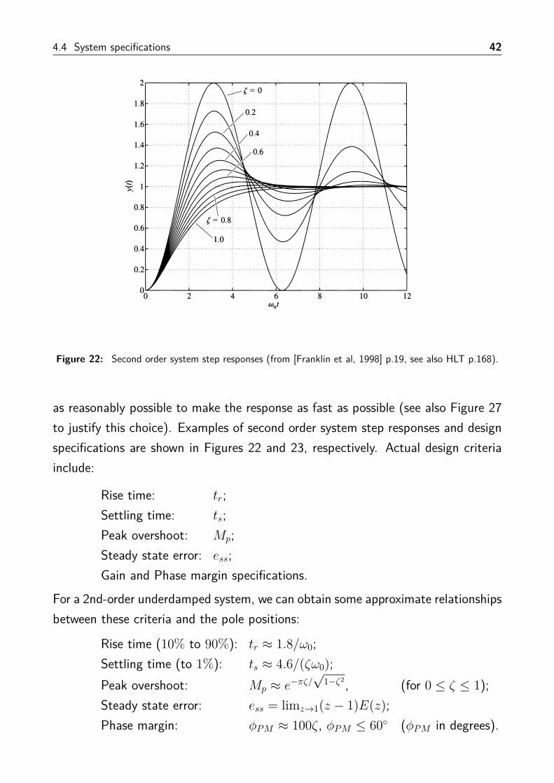
Figure 22: Second order system step responses (from [Franklin et al, 1998] p.19, see also HLT p.168).

as reasonably possible to make the response as fast as possible (see also Figure 27to justify this choice). Examples of second order system step responses and designspecifications are shown in Figures 22 and 23, respectively. Actual design criteriainclude:

Rise time: tr;Settling time: ts;Peak overshoot: Mp;Steady state error: ess;Gain and Phase margin specifications.

For a 2nd-order underdamped system, we can obtain some approximate relationshipsbetween these criteria and the pole positions:

Rise time (10% to 90%): tr ≈ 1.8/ω0;Settling time (to 1%): ts ≈ 4.6/(ζω0);Peak overshoot: Mp ≈ e−πζ/

√1−ζ2, (for 0 ≤ ζ ≤ 1);

Steady state error: ess = limz→1(z − 1)E(z);Phase margin: φPM ≈ 100ζ, φPM ≤ 60◦ (φPM in degrees).


Figure 23: Step response design criteria (from [Franklin et al, 1998] p.20).

To design a controller so as to meet a given specification in terms of ess, ts, Mp

etc., a number of design techniques (including root locus and frequency responsemethods) exist for placing the z-plane poles at desired locations. However theseare beyond the scope of this course. However, we could verify whether certainspecifications are met; this is illustrated by means of the following example.

Example 7. A continuous system with transfer function G(s) = 1/(s(10s +1)) is controlled by a discrete control system with a ZOH, as shown in Fig-ure 21. The closed loop system is required to have: a step response y(kT )with overshoot Mp < 16% and settling time ts < 10 s; and steady-state errorto a unit ramp ess < 1.Validate the satisfaction of these specifications if the sample interval is T = 1s and controller is

uk = −0.5uk−1 + 13(ek − 0.88ek−1).

1. Determine the pulse transfer function of G(s) plus the ZOH:

G(z) = (1− z−1)Z{G(s)

s

}

= (z − 1)zZ{ 0.1s2(s+ 0.1)

}.

4.4 System specifications 44

From the z-transform tables with T = 1 and a = 0.1 we obtain:

G(z) = (z − 1)z

z((0.1− 1 + e−0.1)z + (1− e−0.1 − 0.1e−0.1)

)0.1(z − 1)2(z − e−0.1)

= (0.1− 1 + e−0.1)z + (1− e−0.1 − 0.1e−0.1)0.1(z − 1)(z − e−0.1)

= 0.0484(z + 0.9672)(z − 1)(z − 0.9048) .

2. Determine the controller transfer function D(z): Using the linearity anddelay properties of the z-transform, we obtain

D(z) = U(z)E(z) = 13(1− 0.88z−1)

(1 + 0.5z−1) = 13(z − 0.88)(z + 0.5) .

3. Verify steady state error specification. The transfer function from r to eis given by

E(z)R(z) = 1

1 +D(z)G(z) .

and the steady state error is ess = limk→∞ ek. From the z-transform ofa ramp (see z-transform tables) we obtain that

R(z) = Tz

(z − 1)2 .

By the final value theorem property of the z-transform we thus have that

ess = limz→1

(z − 1)E(z) = limz→1

{(z − 1) Tz

(z − 1)21

1 +D(z)G(z)}

= limz→1

Tz

(z − 1)(1 +D(z)G(z)) , [poles of (z − 1)E(z) in unit circle]

= 1− 0.90480.0484(1 + 0.9672)D(1)

≈ 1D(1) = (1 + 0.5)

13(1− 0.88) = 0.96.

Therefore, ess < 1 as required.

4. Translating the specification on overshoot and settling time into con-straints on the poles of the transfer function from r to y, we obtain:

overshoot: Mp < 16% =⇒ ζ > 0.5;settling time: ts < 10 =⇒ ζω0 > 0.46⇒ radius of poles < 0.63.


The transfer function from r to y is given by

Y (z)R(z) = D(z)G(z)

1 +D(z)G(z) .

It has the following two dominant poles:

z = −0.050± j0.304 = re±jθ

r = |−0.050 + j0.304| = 0.31;θ = tan−1(0.304/0.05) = 1.73.

Notice that, the roots of 1 + D(z)G(z) = 0, are z = 0.876, −0.050 ±j0.304. However the transfer function Y (z)

R(z) has a zero at z = 0.88which effectively cancels the pole at z = 0.876.

By the dominant poles are we have that the specification r < 0.63 issatisfied. Finally, to check that ζ > 0.5, by p. 40 we have that

r = e−ζω0T

θ = ω0T√

1− ζ2

=⇒ ζ√1− ζ2 = ln(1/r)

θ= 0.680 =⇒ ζ = 0.56.

Hence, the controller meets the specifications, as shown by the closedloop step response in Figure 24.

0 1 2 3 4 5 6 7 8 9 10−1.5

−1

−0.5

0

0.5

1

1.5

Time (sec)

Out

put y

and

inpu

t u/1

0

Figure 24: Step response, –+– = output y, –o– = input u× 0.1.

4.5 Summary 46

4.5 Summary


• The pulse response of a 2nd order system is investigated as the radius andargument of its z-plane poles are varied.

• For a sampled data system with a ZOH:

if s = pi is a pole of G(s), then z = epiT is a pole of G(z).

• The locus of s = σ + jω under the mapping z = esT is considered:

. the left half plane (σ < 0) maps to the unit disk (|z| < 1);

. s-plane poles with damping ratio ζ, natural frequency ω0 map to z-planepoles with |z| = e−ζω0T , arg(z) =

√1− ζ2ω0T .

• Design specifications (rise time, settling time, overshoot) translate into con-straints on the ζ and ω0 values of the dominant closed loop poles, that canbe verified for the designed controller.

47 Discrete time linear systems in state space form


We have already seen that discrete time systems emanate from continuous onesvia sampling. In particular, in the previous chapters we focused on such systemsthat are linear, analyzed them and discussed their stability properties by means oftransfer functions. Here, we will revisit the problem of analyzing discrete time linearsystems, but we will do so directly in the discrete time domain.

To this end, this chapter will address the following problems:

1. Provide a unified modelling formalism to represent discrete time linear systems,referred to as state space form.

2. We will provide an explicit characterization of solutions to discrete time linearsystems and discuss how these can be computed.

3. We will discuss how stability can be inferred directly from the system’s statespace representation, without resorting to poles and transfer functions.

5.1 State space representation

Consider a generalization of the plant that is shown in Figure 2, that may havemultiple inputs, encoded by the vector u(t) ∈ Rm, and multiple outputs, encodedby the vector y(t) ∈ Rp. Rather than describing the plant by means of a transferfunction, we have already seen in earlier lectures of A2 Introduction to ControlTheory that, if it is given by a continuous time linear and time-invariant systemwith an input vector u(t) ∈ Rm and an output vector y(t) ∈ Rp, then we canequivalently represent it in the so called state space form. Specifically, the statespace form of a given plant is given by

x(t) = Ax(t) + Bu(t),y(t) = Cx(t) + Du(t).

Vector x(t) ∈ Rn denotes the so called system state that acts as an “internal” vec-tor, whose elements correspond to physical quantities that change over time, hencetheir evolution is described by means of ordinary differential equations (ODEs).

5.1 State space representation 48

Stacking these ODEs together gives rise to the first of the equations in the statespace description above. The second equation is an algebraic one and encodesthe information that is available in the output of the system by means of sensormeasurements. These equations together constitute the state space form of a con-tinuous, time-invariant, linear system and are fully parameterized by the matricesA ∈ Rn×n, B ∈ Rn×m, C ∈ Rp×n and D ∈ Rp×m.

With reference to Figure 2, we would like to analyze the sampled data system withinput uk and output yk, where k ≥ 0 corresponds to any given sampling instance.Recall that for any t ∈ [kT, (k + 1)T ] the state solution of the continuous timelinear system can be written as

x(t) = eA(t−kT )xk +∫ tkTeA(t−τ)Bu(τ)dτ,

where xk = x(kT ) plays the role of the initial condition of the state over thesampling interval under consideration. As the initial condition is not x(0), the termkT appears in the exponential of the first term and the lower limit of the integral inthe second term, to account for the fact that the initial time of the state evolutionis no longer zero but kT . Notice that between consecutive sampling instances kTand (k + 1)T , the control input remains constant to uk as an effect of the ZOH,i.e., we have that

u(t) = uk for all t ∈ [kT, (k + 1)T ).

Evaluating the state solution at t = (k + 1)T and setting xk+1 = x((k + 1)T ), wehave that

xk+1 = eATxk + ∫ (k+1)T

kTeA((k+1)T−τ)Bdτ

uk[change of variables: τ ← τ − kT ]

= eATxk + ∫ T

0eA(T−τ)Bdτ

uk.Moreover, the output equation at the sampled time instances is given by

yk = Cxk + Duk.

where yk = y(kT ). Combining the derived equations for the (next) state xk+1 andthe output yk as functions of xk and uk we obtain the state space description of asampled data, discrete time linear system. This is summarized below.


A sampled data, discrete time linear system is said to be in state space formif it can be written as

xk+1 = Axk +Buk,

yk = Cxk +Duk,

where A = eAT ∈ Rn×n, B = ∫ T0 e

A(T−τ)Bdτ ∈ Rn×m, C = C ∈ Rp×n andD = D ∈ Rp×m. Matrices (A, B, C, D) correspond to the state space formof the continuous time, linear, time-invariant system prior to sampling, and Tdenotes the sampling period.

Example 8. Consider a plant given by the continuous time linear system

x(t) = −x(t) + u(t),y(t) = x(t).

The system is already in state space form with A = −1, B = 1, C = 1 andD = 0 (all scalars). To compute the state space description of the associatedsampled data system with sampling period T , we need to determine matrices(A,B,C,D). To this end, notice that C = C = 1 and D = D = 0, while

A = eAT = e−T ,

B =∫ T

0eA(T−τ)Bdτ =

∫ T0eτ−Tdτ = 1− e−T .

Therefore, the associated discrete time system is given by

xk+1 = e−Txk + (1− e−T )uk,yk = xk.

For the case where unlike the preceding example the system is non-scalar, given acontinuous time state space description we can construct the discrete time one bymeans of the following two steps:

1. Step 1: Compute the matrix exponential eAT . This can be computed asdiscussed in earlier lectures of A2 Introduction to Control Theory. In par-ticular, if A is diagonalizable, we can compute the matrix exponential as

5.2 Solutions to discrete time linear systems 50

eAT = WeΛTW−1, where W is a matrix with the eigenvectors of A as itscolumns (invertible as for diagonalizable matrices eigenvectors are linearly in-dependent) and Λ is a diagonal matrix with the eigenvalues of A as the diagonalentries. Since Λ is diagonal, computing eΛT becomes then easier as it involvescomputing scalar exponentials corresponding to the entries of Λ, i.e.,

eΛT =

eλ1T 0 . . . 00 eλ2T . . . 0... ... . . . ...0 0 . . . eλnT

where λ1, . . . , λn are the eigenvalues of A.

2. Step 2: Compute the integral ∫ T0 eA(T−τ)Bdτ . This should be performedelementwise for every entry of the matrix eA(T−τ)B that appears in the inte-grand, which in turn involves the matrix exponential.

5.2 Solutions to discrete time linear systems

Consider a discrete time linear system in state space form, and an arbitrary initialstate x0. For a given sequence of inputs uk, k = 1, . . ., we can provide an explicitcharacterization of the solution to such systems. In particular, the state xk andoutput yk solution for any instance k, are given by

xk =

zero input transition︷︸︸︷Akx0 +

zero state transition︷︸︸︷k−1∑i=0

Ak−i−1Bui

yk = CAkx0︸︷︷︸zero input response

+k−1∑i=0

CAk−i−1Bui +Duk.

︸︷︷︸zero state response

We will not prove that the expressions for xk and yk satisfy the difference andoutput equation, respectively; this can be achieved using induction. Notice that


once xk is computed, the output solution can be directly determined by means ofyk = Cxk + Duk. The first term in the state solution is the so called zero inputtransition, i.e., the solution of the system if it was autonomous, or in other wordsif ui = 0 for all i. The second term is the so called zero state transition, and it isa discrete time convolution corresponding to the solution of the system when theinitial state is zero. The interpretation of the zero input response and the zero stateresponse is analogous, referring to the output yk instead.

These solutions are in direct correspondence with the ones for continuous timelinear systems; the only difference is that the convolution integral is replaced witha summation involved in discrete time convolution, while the matrix exponential isreplaced by Ak. The latter is the term that is the most difficult to compute so thatwe determine the state output solutions xk and yk. We discuss its computationseparately for systems with a diagonalizable and a non-diagonalizable matrix A.

5.2.1 Diagonalizable matrices

A matrix is called diagonalizable if its eigenvectors are linearly independent. Wehave the following sufficient conditions for a matrix to be diagonalizable:

1. If a matrix A ∈ Rn×n has distinct eigenvalues (i.e., λi 6= λj for all i 6= j), thenits eigenvectors are linearly independent.

2. If a matrix is symmetric (A = A> ∈ Rn×n), then i) its eigenvalues are real; ii)its eigenvectors are orthonormal (hence linearly independent).

Diagonalizability is a desirable property as, if a matrix A is diagonalizable, it canbe decomposed as

A = WΛW−1,

where W is a matrix whose columns are the eigenvectors of A (invertible since theeigenvectors are linearly independent), and Λ is a diagonal matrix whose diagonalentries correspond to the eigenvalues of A. For discrete time linear systems witha diagonalizable matrix A the quantity Ak that appears in the expressions for thestate and output solutions can be computed efficiently in closed form.

5.2 Solutions to discrete time linear systems 52

Fact 4. Consider a discrete time linear system with matrix A ∈ Rn×n beingdiagonalizable, thus admitting a decomposition A = WΛW−1. We then havethat

Ak = WΛkW−1,

where Λk =

λk1 0 . . . 00 λk2 . . . 0... ... . . . ...0 0 . . . λkn

, with λi being the i-th eigenvalue of A.

Proof: We show this by means of induction:

1. Base case (k = 0): We have that WΛ0W−1 = WW−1 = I = A0, hencethe base case is trivially satisfied.

2. Induction hypothesis: Assume the statement holds true for an arbitraryk, i.e., Ak = WΛkW−1.

3. Show the claim for the (k + 1)-th case: By the induction hypothesis wehave that Ak = WΛkW−1. Hence,

Ak+1 = AkA = WΛk��

��:IW−1W ΛW−1 = WΛk+1W−1.

Example 9. Consider a discrete time linear system with difference equation

xk+1 = Axk =1

212

0 1

xk.

Compute the zero input transition if the initial state is x0 =−1

1

.

Step 1: Compute the eigenvalues of A. Since the matrix is triangular, theeigenvalues correspond to the diagonal elements, i.e., λ1 = 1

2 and λ2 = 1.Since the eigenvalues are distinct we infer that A is diagonalizable.Step 2: Compute the eigenvectors of A. By direct calculation we obtain that

corresponding to λ1 : w1 =10

, corresponding to λ2 : w2 =11

.


Step 3: Since A is diagonalizable, we can write it as A = WΛW−1, where

Λ =1

2 00 1

, W =1 10 1

and W−1 =1 −10 1

.We then have that the zero state transition is given by

xk = Akx0 = WΛkW−1x0

=1 10 1

1

2k 00 1

1 −10 1

−1

1

=1− 1

2k−1

1

.

Notice that as k →∞ the state tends to11

.

5.2.2 Non-diagonalizable matrices

A matrix A ∈ Rn×n is called non-diagonalizable if the number of linearly indepen-dent eigenvectors is strictly lower than n. Moreover, not all of its eigenvalues aredistinct, and at least one of them would be repeated. If the matrix A of a givendiscrete time linear system is non-diagonalizable, then we can no longer decomposeA using the eigenvector matrix W as this will no longer be invertible (recall thatthe columns of W are the eigenvectors).

Computing Ak for non-diagonalizable matrices with generic structure is a difficulttask; it requires resorting to the so called Jordan form and will not be addressed inthese notes. However, for a particular class of non-diagonalizable matrices comput-ing Ak can be performed efficiently. We illustrate this by means of an example.

Example 10. Consider the matrix

A =

0 1 00 0 10 0 0

.

5.3 Stability of discrete time linear systems 54

The diagonal elements of A correspond to its eigenvalues, hence A has arepeated eigenvalue λ = 0 with multiplicity equal to 3. To decide whether Ais diagonalizable we have to compute its eigenvectors. Using λ = 0 we obtainonly one eigenvector, i.e.,

0 1 00 0 10 0 0

w1

w2

w3

= 0 ⇒ w2 = w3 = 0, eigenvector: w =

100

Since we only have 1 < 3 linearly independent eigenvectors, A is non-diagonalizable.However, notice that we can still compute Ak efficiently, as A3 = 0 and as aresult, Ak = 0 for all k ≥ 3.

Matrices that exhibit this property (excluding the trivial case of a zero matrix), i.e.,there exists some integer k such that Ak = 0 for all k ≥ k, are called Nilpotent.Triangular n×n matrices with zeros along the main diagonal are all Nilpotent withk ≤ n. For Nilpotent matrices the state solution satisfies

xk = Akx0 = 0 for all k ≥ k.

In other words, the state of the system becomes zero in finite time (k time instances)and stays there from then on. Therefore, for non-diagonalizable but Nilpotent ma-trices A the system’s state solution can be easily computed. Despite the analogiesbetween continuous and discrete time linear systems, this behaviour is not encoun-tered in continuous time systems.

5.3 Stability of discrete time linear systems

In this section we will investigate the stability properties of discrete time linearsystems with no inputs, i.e., systems governed by

xk+1 = Axk.

In other words, we will analyze the so called zero input transition of the statesolution, namely xk = Akx0. However, stability is related to the limiting behaviour


of the system state xk as k → ∞. In particular, we will investigate the stabilityproperties of the equilibrium point xk = 0, as if the state becomes zero for somek, we would have that all subsequent states would be zero as well since xk+1 =Axk = 0. We consider the following notions of stability:

1. Stability: A system is called stable? if we can stay arbitrarily close enough to0 if we start sufficiently close to it.

2. Asymptotic stability: A system is called asymptotically stable if it is stable,and approaches 0 as time tends to infinity, i.e., limk→∞ ‖xk‖ = 0. In otherwords, not only we stay close to 0, but also converge to it.

We then say that a system that is not stable is unstable. We will investigate thesenotions of stability for systems of the form xk+1 = Axk, separately for diagonalizableand non-diagonalizable A matrices.

5.3.1 Diagonalizable matrices

In the case where A is diagonalizable, following the procedure outlined in Fact 4,we can represent the state solution of the system (i.e., the zero input transition inthe absence of inputs) for any k as

xk = Akx0 = WΛkW−1x0.

It follows then that Ak (and as result xk) will be a linear combination of terms λki ,i = 1, . . . , n, where λ1, . . . , λn are the eigenvalues of A. The coefficients of thislinear combination would then depend on the eigenvectors that appear in W andthe initial state, and would dictate how the terms λki , i = 1, . . . , n, mix.

It follows then that the eigenvalues affect the limiting behaviour of the state. Eigen-values are in general complex, hence we can represent them as λi = σi+ jωi, whichimplies that |λi| =

√σ2i + ω2

i . It can be then observed that

• If |λi| = 1 then |λi|k = 1 for all k.?Formally, a system is called stable if for all ε > 0, there exists δ > 0 such that if ‖x0‖ ≤ δ then

‖xk‖ ≤ ε for all k ≥ 0.

5.3 Stability of discrete time linear systems 56

• If |λi| < 1 then limk→∞ |λi|k = 0.

• If |λi| > 1 then limk→∞ |λi|k =∞.

The relationships above sumarize the limiting behaviour for one of the terms thatwould appear in the state solution, i.e., the one related to λki . However, the statesolution would be a mix of such terms corresponding to the different eigenvalues ofA. We are then able to make the following statements related to stability.

Fact 5 (Stability of xk+1 = Axk with diagonalizable A). Consider a discretetime linear system of the form xk+1 = Axk with A ∈ Rn×n diagonalizable.Denote by λi, i = 1, . . . , n, the eigenvalues of A. We then have that thesystem is

• Stable (for all initial conditions) if and only if |λi| ≤ 1 for all i = 1, . . . , n.

• Asymptotically stable (for all initial conditions) if and only if |λi| < 1 forall i = 1, . . . , n.

• Unstable (for some initial conditions) if and only if there exists i suchthat the corresponding eigenvalue has |λi| > 1.

Note that it suffices that at least one eigenvalue has magnitude greater than onefor the system to be unstable. Moreover, if at least one eigenvalue has magnitudeequal to one, while all other ones have magnitude strictly lower than one, then thesystem is stable but not asymptotically stable. The reason is that the contributionof that particular eigenvalue in the state solution is bounded (constant or periodic,hence we only stay “close” to zero but do not converge to it). Notice that this isthe case in Example 9 as one of the eigenvalues is equal to one, hence in the limitthe state does not tend to zero for the particular choice of the initial condition.

These implications of stability are in direct correspondence with the less formalstability observations according to the poles of the system’s transfer function. Inparticular, poles and eigenvalues convey the same information about stability. Infact, a pole is also an eigenvalue of the system’s A matrix; vice verca, if the thereare no pole-zero cancellations, an eigenvalue is also a pole of the system’s transferfunction.


5.3.2 Non-diagonalizable matrices

In the case where A is non-diagonalizable but Nilpotent, then the state reaches zeroin finite time and stays there afterwards (see Example 11), hence we have stabilityand in fact we achieve this in finite time. However, for non-diagonalizable matriceswith generic structure, eigenvalues offer less information as far as determining thesystem’s stability is concerned. To see this, recall first that for non-diagonalizablematrices at least one eigenvalue will be repeated. If for all eigenvalues |λi| ≤1, i = 1, . . . , n, but the repeated eigenvalue is such that |λi| = 1 then, unlikediagonalizable matrices, the response may be stable or unstable according to theinitial condition (and how this relates to eigenvectors). We illustrate this by meansof an example.

Example 11. Consider the system

xk+1 = Axk =1 10 1

xk.The diagonal elements of A correspond to its eigenvalues, hence A has arepeated eigenvalue λ = 1 with multiplicity equal to 2. To decide whether Ais diagonalizable we have to compute its eigenvectors. Using λ = 1 we obtainonly one eigenvector, i.e.,1 1

0 1

w1

w2

=w1

w2

⇒ w2 = 0, eigenvector: w =10

Since we only have 1 < 2 linearly independent eigenvectors, A is non-diagonalizable.By computing a few powers and observing the patterm, notice that for allk ≥ 1

Ak =1 k

0 1

.For different initial states we observe the following:

xk = Akx0 =1 k

0 1

10

=10

,

xk = Akx0 =1 k

0 1

01

=k1

.

5.4 Summary 58

Notice that the first initial state (aligned with the eigenvector) leads to astable solution, while for the second initial state ‖xk‖ tends to inifinity as kincreases.

However, looking into the eigenvalues we can still claim the following.

Fact 6 (Stability of xk+1 = Axk with non-diagonalizable A). Consider adiscrete time linear system of the form xk+1 = Axk with A ∈ Rn×n non-diagonalizable. Denote by λi, i = 1, . . . , n, the eigenvalues of A (at least oneof them would be repeated). We then have that the system is

• Asymptotically stable (for all initial conditions) if and only if |λi| < 1 forall i = 1, . . . , n.

• Unstable (for some initial conditions) if there exists i such that the cor-responding eigenvalue has |λi| > 1.

5.4 Summary


• Given a continuous time linear system with state space description encoded by(A, B, C, D), the associated sampled data (with sampling period T ), discretetime linear system can be written in state space form as

xk+1 = Axk +Buk,

yk = Cxk +Duk,

where A = eAT ∈ Rn×n, B = ∫ T0 e

A(T−τ)Bdτ ∈ Rn×m, C = C ∈ Rp×n andD = D ∈ Rp×m.

• The state and output solutions to discrete linear systems are, respectively,


given by

xk = Akx0 +k−1∑i=0

Ak−i−1Bui,

yk = CAkx0 +k−1∑i=0

CAk−i−1Bui +Duk.

It was shown that for

– Diagonalizable A: Ak = WΛkW−1, where W includes the eigenvectorsof A as columns, while Λ is a diagonal matrix with the eigenvalues of Aon its diagonal.

– Non-diagonalizable A: For the particular class of Nilpotent matrices, Ak =0 for some integer k.

• The stability of discrete time systems of the form xk+1 = Axk was analyzedand conditions to guarantee stability based on the eigenvalues of matrix A

were derived. Irrespective of whether A is diagonalizable or not, if λ1, . . . , λn

denote its eigenvalues, we can claim that:

– Asymptotically stable system if and only if |λi| < 1 for all i = 1, . . . , n.

– Unstable system if there exists i such that |λi| > 1.

60

6 Appendix: The inverse z-transform

We provide in this appendix a formal definition of the inverse z-transform?. Tothis end, consider a discrete time signal f(kT ), k = 0, 1, . . ., and its z-transform(assuming that all values corresponding to negative indices are zero)

F (z) = Z{f(kT )

}= Z

{fk}

=∞∑k=0

fk z−k.

The inverse z-transform is defined as

f(kT ) = Z−1{F (z)}

= 12πj

∮zk−1F (z) dz,

where the contour encircles the region of convergence of F (z) (recall that the z-transform is defined for a particular region of z values where the infinite series sumconverges).

To calculate the integral is rather not easy, and relies on the following result whichis based on Cauchy’s residue calculus. Consider some function G(z) and let zi bethe i-th pole of G(z) which is of order n. The function (z − zi)nG(z) is thenanalytic at zi and as such we can obtain its Taylor series expansion as

(z − zi)nG(z) = A−n + A−n+1(z − zi) + . . .+ A−1(z − zi)n−1 + A0(z − zi)n + . . .

A−1 is then defined as the residue of G(z) at zi, and is denoted as Res(zi). Forsingle poles (i.e., n = 1) the residue is the constant term of the Taylor seriesexpansion. According to Cauchy’s residue calculus we then have that

12πj

∮G(z) dz =

∑i

Res(zi), [Cauchy’s equation]

if G(z) is analytic on the closed contour where the integral is defined, as well as inits interior, except from a finite number of singularities.

Proof of the inverse z-transform: We will show that the right-hand side of theinverse z-transform is indeed f(kT ). To achieve this consider the right-hand sideof the inverse z-transform, and substitute F (z) according to its definition, i.e.,

12πj

∮zk−1F (z) dz = 1

2πj∮zk−1

∞∑`=0

f`z−` dz

= 12πj

∞∑`=0

f`∮zk−1−` dz,

?[Franklin et al, 1998] §4.6.2

61 Appendix: The inverse z-transform

where the integral and the summation can be exchanged as the integration contouris taken in the region where F (z) is convergent.

Letting G(z) = zk−1−`, three cases can be distinguished: i) if k − 1 − ` ≥ 0 thenG(z) has no poles inside the contour, hence there are no residue. ii) if k − ` < 0then G(z) has a pole at zero of order `+ 1− k. This implies that z`+1−kG(z) = 1would be constant, and according to Taylor’s expansion the residue A−1 would bezero. iii) if ` = k then G(z) has a single pole at zero. This implies then thatzG(z) = 1, but the residue A−1 is now 1, the constant term of the Taylor seriesexpansion. Therefore, all terms in the summation preceding the integral would bezero but for the case ` = k where ∑

i Res(zi) = 1, and by Cauchy’s equation withG(z) = zk−1−` we have that 1

2πj∮zk−1−` dz = 1. Hence, the right-hand side of the

inverse z-transform definition becomes1

2πj∮zk−1F (z) dz = f(kT ),

which is indeed the discrete-time signal f(kT ).

Example 12. Let F (z) = zz−1 (with convergence region |z| > 1). We will

show that its inverse z-transform is

f(kT ) =

1, k ≥ 0,0, k < 0.

i.e., the unit step signal.Consider the inverse z-transform

fk = Z−1{F (z)}

= 12πj

∮ z

z − 1zk−1 dz = 1

2πj∮ zk

z − 1 dz,

where the contour encircles the region |z| > 1, where convergence for F (z) isensured.Consider first the case k ≥ 0. Let G(z) = zk

z−1 and notice that it has onlyone single pole at one. Hence, by the Taylor series expansion of (z− 1)nG(z)with n = 1,

(z − 1)G(z) = zk = 1 + k(z − 1) + . . .

with the residue A−1 being equal to 1. By Cauchy’s equation we then havethat 1

2πj∮G(z)dz = 1, which in turn implies that fk = 1 for all k ≥ 0.

62

Consider now the case k < 0. Let G(z) = zk

z−1 and notice that it has a singlepole at one and a pole at zero of order k. For the pole at one, the Taylorexpansion is the same as before, and the residue is 1. For the pole at zero, bythe Taylor series expansion of znG(z) with n = −k (recall k is negative),

z−kG(z) = 1z − 1 = −1(1 + z−1 + z−2 + . . .).

The residue is −1 irrespective of the value of k. Therefore, Res(1)+Res(0) =1− 1 = 0. As a result, by Cauchy’s equation we have that 1

2πj∮G(z)dz = 0,

which in turn implies that fk = 0 for all k < 0.Therefore, we have shown that the inverse z-transform of F (z) = z

z−1 is theunit step as expected from the inverse z-transform tables. However, it shouldbe noted that knowledge of the region of convergence for the z-transform (inthat case |z| > 1) is essential for the determination of the integral’s contour,and hence the correct calculation of the inverse transform.

a2 introduction to control theory: discrete time linear

Documents