Linear Assignment Problems and Extensions ∗

Rainer E. Burkard † Eranda Cela †

Abstract

This paper aims at describing the state of the art on linear assignment problems(LAPs). Besides sum LAPs it discusses also problems with other objective functionslike the bottleneck LAP, the lexicographic LAP, and the more general algebraic LAP. Weconsider different aspects of assignment problems, starting with the assignment poly-tope and the relationship between assignment and matching problems, and focusingthen on deterministic and randomized algorithms, parallel approaches, and the asymp-totic behaviour. Further, we describe different applications of assignment problems,ranging from the well know personnel assignment or assignment of jobs to parallel ma-chines, to less known applications, e.g. tracking of moving objects in the space. Finally,planar and axial three-dimensional assignment problems are considered, and polyhedralresults, as well as algorithms for these problems or their special cases are discussed.The paper will appear in the Handbook of Combinatorial Optimization to be publishedby Kluwer Academic Publishers, P. Pardalos and D.-Z. Du, eds.

Keywords: assignment, assignment polytope, linear assignment problems, al-gorithms, asymptotic behavior.

AMS-classification: 90C27, 68Q25, 90C05

Contents

1 Assignments 3

2 Linear Sum Assignment Problems (LSAPs) 8

3 Algorithms for the LSAP 113.1 Primal-Dual Algorithms . . . . . . . . . . . . . . . . . . . . . . . . . . . . . . . . . . 123.2 Simplex-Based Algorithms . . . . . . . . . . . . . . . . . . . . . . . . . . . . . . . . . 173.3 Other Algorithms . . . . . . . . . . . . . . . . . . . . . . . . . . . . . . . . . . . . . . 213.4 On Parallel Algorithms . . . . . . . . . . . . . . . . . . . . . . . . . . . . . . . . . . . 23

4 Asymptotic Behavior and Probabilistic Analysis 25

5 Bottleneck Assignment Problems 29

6 Assignment Problems with Other ObjectiveFunctions 32

∗This research has been supported by the Spezialforschungsbereich F 003 “Optimierung und Kontrolle”,

Projektbereich Diskrete Optimierung.†Technische Universitat Graz, Institut fur Mathematik B, Steyrergasse 30, A-8010 Graz, Austria.

1

7 Available computer codes and test instances 35

8 Multidimensional Assignment Problems 368.1 General Remarks and Applications . . . . . . . . . . . . . . . . . . . . . . . . . . . . 368.2 Axial 3-Dimensional Assignment Problems . . . . . . . . . . . . . . . . . . . . . . . . 388.3 Planar 3-Dimensional Assignment Problems . . . . . . . . . . . . . . . . . . . . . . . 42

References

2

1 Assignments

Assignment problems deal with the question how to assign n items (e.g. jobs) to n machines(or workers) in the best possible way. They consist of two components: the assignment asunderlying combinatorial structure and an objective function modeling the ”best way”.

Mathematically an assignment is nothing else than a bijective mapping of a finite setinto itself, i.e., a permutation. Assignments can be modeled and visualized in differentways: every permutation φ of the set N = {1, . . . , n} corresponds in a unique way to apermutation matrix Xφ = (xij) with xij = 1 for j = φ(i) and xij = 0 for j 6= φ(i). We canview this matrix Xφ as adjacency matrix of a bipartite graph Gφ = (V,W ;E), where thevertex sets V and W have n vertices, i.e., |V | = |W | = n, and there is an edge (i, j) ∈ E iffj = φ(i), cf. Fig. 1.

φ =

(

1 2 3 43 2 4 1

)

Xφ =

0 0 1 00 1 0 00 0 0 11 0 0 0

4

1

2

3

4

1

2

3

Figure 1: Different representations of assignments

The set of all assignments of n items will be denoted by Sn and has n! elements. Wecan describe this set by the following equations called assignment constraints

n∑

i=1

xij = 1 for all j = 1, . . . , n

n∑

j=1

xij = 1 for all i = 1, . . . , n (1)

xij ∈ {0, 1} for all i, j = 1, . . . , n

Let A be the coefficient matrix of the system of equations (1). Matrix A is totally unimodu-lar , i.e., every square submatrix of A has a determinant of value +1, −1 or 0. By replacingthe conditions xij ∈ {0, 1} by xij ≥ 0 in (1), we get a doubly stochastic matrix . The set ofall doubly stochastic matrices forms the assignment polytope PA. Due to a famous resultof Birkhoff [36], the assignment polytope PA is the convex hull of all assignments:

Theorem 1.1 (Birkhoff [36], 1946)The vertices of the assignment polytope correspond uniquely to permutation matrices.

Differently said every doubly stochastic matrix can be written as convex combination ofpermutation matrices. Further properties of the assignment polytope are summarized inthe following theorem:

Theorem 1.2 (Balinski and Russakoff [22], 1974)Let PA be the assignment polytope for assignments on a set N with n elements. Then

3

1. dim PA = (n− 1)2.

2. Every of the n! vertices of PA coincides with∑n−1k=0

(nk

)

(n− k − 1)! different edges.

3. Any two vertices are joined by a path with at most two edges, i.e., the diameter of PAis 2.

4. PA is Hamiltonian.

A polytope is Hamiltonian, if there exists a closed path along its edges which visits everyvertex of the polytope just once.

Consider a bipartite graph G = (V,W ;E) with vertex sets V = {v1, v2, . . . , vn} andW = {w1, w2, . . . , wn}, and edge set E. A subset M of E is called a matching , if everyvertex of G is incident with at most one edge from M . The cardinality of M is calledcardinality of the matching. The maximum matching problem asks for a matching with asmany edges as possible. A matching M is called a perfect matching , if every vertex of G isincident with exactly one edge from M , i.e., |M | = n. Evidently, every perfect matching isa maximum matching and corresponds to an assignment. The number of different perfectmatchings in a bipartite graph G is given by the permanent of the corresponding n × nadjacency matrix A = (aij) defined by

aij :=

{

1 if (vi, wj) ∈ E

0 if (vi, wj) 6∈ E

The permanent per(A) is defined by

per(A) :=∑

φ∈Sn

a1φ(1)a2φ(2) . . . anφ(n).

The numerical evaluation of a permanent (and the determination of the number of differentperfect matchings in a graph G) is #P-complete (Valiant [162]). This implies that thedetermination of the number of different perfect matchings in G is at least as hard as anyNP-complete problem. The following theorem due to Hall [99] states a necessary andsufficient condition for the existence of a perfect matching in a bipartite graph. Halmosinterpreted such a perfect matching as a marriage between ladies in the set V and gentlemenin set W , and due to this interpretation Hall’s theorem is known as Marriage theorem. Fora vertex v ∈ V let N(v) be the set of its neighbors, i.e., the set of all vertices w ∈W whichare connected with v by an edge in E. Thus N(v) contains the friends of v. Moreover, forany subset V ′ of V let N(V ′) =

⋃

v∈V ′ N(v).

Theorem 1.3 (Marriage theorem, Hall [99], 1935)Let G = (V,W ;E) be a bipartite graph. G contains an assignment (perfect matching,marriage) if and only if |V | = |W | and for all subsets V ′ of V

|V ′| ≤ |N(V ′)| (Hall condition)

This theorem says that by checking the exponentially many subsets V ′ of V we can de-cide, whether the graph G has a perfect matching or not. Hopcroft and Karp [103] gavea polynomial-time algorithm to decide this question. They construct a perfect matching,if it exists, in O(|E|

√

|V |) steps. Alt, Blum, Mehlhorn and Paul [9] improved the com-plexity for dense graphs by a fast adjacency matrix scanning technique and obtain anO(|V |1.5

√

|E|/ log |V |) implementation for the Hopcroft-Karp algorithm.

4

The decision can also be made faster by a randomized algorithm which is a Monte-Carloapproach. This algorithm may err with an arbitrarily small probability in the case that itsoutput does not confirm the existence of a matching. The randomized algorithm is based onthe relationship between the determinant of the Tutte matrix of a graph and the existenceof a perfect matching (Tutte [161]). The Tutte matrix A(x) = (xij) of an (undirected)graph G = (V,E) is a skew symmetric matrix with variable entries xij , xij = −xji, wherexij = xji ≡ 0, if (i, j) is not an edge of G.

Theorem 1.4 (Tutte [161], 1947)Let A(x) be the Tutte matrix of graph G = (V,E). There exists a perfect matching in G, ifand only if the determinant of A(x) is not identically equal to 0.

A randomized algorithm to decide whether G has a perfect matching can be obtainedby generating xij uniformly at random from {1, 2, . . . , 2|E|} and by computing the deter-minant of the corresponding Tutte matrix A(x), and eventually repeating this process afixed number of times. The probability of an error can be estimated by applying a resultof Schwarz [157] on the probability of hitting roots of a given polynomial. By applyingSchwartz’s results one gets that the error probability of the above randomized algorithm isequal to (1/|E|)r , where r is the number of repetitions and |E| is the number of edges ofG. Since an n × n determinant can be evaluated in O(n2.376) time (see Coppersmith andVinograd [60]), and by assuming constant time for the generation of a random number, thisrandomized algorithm is faster than the best existing deterministic algorithm, at least inthe case of dense graphs. This procedure does, however, not compute a perfect matching,it just decides - with an arbitrarily small probability of error - whether the given graph hasone. To compute a perfect matching in G we may delete edges of G and test whether theremaining graph has a perfect matching. This procedure is repeated until no further edgescan be deleted without destroying all perfect matchings in the remaining graph. Obviously,this remaining graph is then a perfect matching. Instead of this naive algorithm Mulmuley,Vazirani and Vazirani [129] propose a parallel algorithm which performs a matrix inversiononly once. The basic idea relies on assigning random weights to the edges of the graph andon generating the random variables xij in the Tutte matrix so that the perfect matchingwith minimum weight is unique. Then, an easy-to-check condition is given for the member-ship of a certain edge to this minimum weighted perfect matching. This algorithm requiresO(|V |3.5|E|) processors to find a perfect matching in O(log2 |V |) time.

Cechlarova [57] gives a necessary and sufficient condition that a bipartite graph Gcontains a unique perfect matching. This is the case, if the rows and columns of theadjacency matrix can be permuted by φ such that in the permuted matrix (aφ(i)φ(j)) all1 entries lie on the main diagonal or below. Cechlarova shows that graphs with a uniqueperfect matching can be recognized in O(|E|) time and the same time complexity is neededfor constructing the unique perfect matching.

The maximum matching problem is particularly easy to solve in so-called convex bipar-tite graphs (Glover [89]). A bipartite graph G = (V,W ;E) with vertex sets V and W andedge set E is convex , if for all i, k, i < k, and j

(i, j), (k, j) ∈ E ⇒ all (i+ 1, j), . . . , (k − 1, j) ∈ E.

Glover described the following simple algorithm for finding a maximum matching in convexbipartite graphs:

1. Compute for every j ∈W the label π(j) := max {i|(i, j) ∈ E}.

5

2. Start with the empty matching M .For i = 1, 2, . . . , |V | do:If there exists an edge (i, j) with unmatched vertex j, then enlarge the matching bythe edge (i, k) with minimum value π(k).

A straightforward implementation of this algorithm has complexity O(n2). Using a methodof Gabow and Tarjan [86] the maximum matching can even be found in linear time. Match-ings in convex graphs are used in the solution of so-called terminal assignment problems.Terminal assignment problems arise in connection with the design of integrated circuits.They can be described as follows: each of n entry terminals positioned on the upper layerof a channel has to be assigned to one of the m exit terminals positioned in the lower layer.The density d(x) of a given assignment at position x is the number of terminals in theupper layer, left to x, which are connected to an exit in the lower layer right to position x,see Fig. 2. The density of an assignment is the maximum of d(x) taken over all positionsx. If there are two upper layers, the density is computed for each upper layer separately

o

x x

d(x d(x)=1)=2

o

Figure 2: An instance of the terminal assignment problem. The densityof this assignment is 2 and is attained at position x0, d(x0) = 2.

and the total density is the maximum of these two densities. In the terminal assignmentproblem the terminals situated in two upper layers are to be assigned such that the resultingchannel routing problem has minimum total density. Rote and Rendl [155] solve the 2-layerterminal assignment problem by a recursive algorithm in linear time using matchings inconvex bipartite graphs.

Flows in networks offer another model to describe assignments. Let G be the bipartitegraph introduced before. We embed G in the network N = (N,A, c) with node set N , arcset A and arc capacities c. The node set N consists of a source s, a sink t and the verticesof V ∪W . The source is connected to every node in V by an arc of capacity 1, every node inW is connected to the sink by an arc of capacity 1, and every edge in E is directed from Vto W and supplied with an infinite capacity. A flow in network N is a function f :A→ IRwith

∑

x∈V ∪W

f(x, y) =∑

x∈V ∪W

f(y, x) , for all y ∈ V ∪W (2)

0 ≤ f(x, y) ≤ c(x, y), for all (x, y) ∈ A (3)

Equalities (2) and (3) are called flow conservation constraints and capacity constraints,

6

respectively. The value z(f) of the flow f is defined as

z(f) :=∑

x∈N

f(s, x) .

1

s t

a

b

c

d

a’

b’

c’

d’

a

b

c

d

a’

b’

c’

d’

11

1

1

1

11 1

11

1

Figure 3: Perfect matching in a bipartite graph and correspondingnetwork flow model. A minimum cut is given by {s, b, b′}. Thdashed edges contribute to the value of the cut.

The maximum network flow problem asks for a flow with maximum value z(f). Obviously, amaximum integral flow in the special network constructed above corresponds to a matchingwith maximum cardinality. A cut in the network N is a subset C of the node set N withs ∈ C and t 6∈ C. The value u(C) of cut C is defined as

u(C) :=∑

x∈C, y 6∈C(x,y)∈A

c(x, y) .

Ford and Fulkerson’s famous Max Flow-Min Cut Theorem [85] states that the value of amaximum flow equals the minimum value of a cut.

This leads immediately to the matching theorem of Konig [116]. Given a bipartitegraph G, a vertex cover (cut) in G is a subset of its vertices such that every edge is incidentwith at least one vertex in this set.

Theorem 1.5 (Konig’s Matching Theorem, 1931)In a bipartite graph the minimum number of vertices in a vertex cover equals the maximumcardinality of a matching.

Let us now translate this theorem in the language of 0-1 matrices. Given a bipartite graphG = (V,W ;E) with |V | = |W | = n, we define an n× n 0-1 matrix B = (bij) as follows

bij :=

{

0 if (i, j) ∈ E

1 if (i, j) 6∈ E

A zero-cover is a subset of rows (columns) of matrix B which contains all 0 elements. Arow (column) which is an element of a zero-cover is called a covered row (covered column).Now we get

Theorem 1.6 There exists an assignment φ with biφ(i) = 0 for all i = 1, . . . , n, if and onlyif the minimum zero cover has n elements.

7

0 0 0∗ 11 0∗ 1 10∗ 0 1 11 0 1 0∗

Figure 4: 0-1 matrix model of a bipartite graph and the corre-sponding minimum vertex cover which corresponds to the cut inFig. 3. An assignment is given by the entries marked by ∗.

A maximum matching corresponds uniquely to a maximum flow in the corresponding net-work N , and therefore to a minimum cut C in this network. From this minimum cut wecan construct a zero-cover in the adjacency matrix: if node i ∈ V of the network does notbelong to cut C, then row i is an element of the zero-cover. Analogously, if node j ∈ Wbelongs to cut C, then column j is an element of the zero-cover.

2 Linear Sum Assignment Problems (LSAPs)

In this section we deal with the classical linear sum assignment problem (LSAP). We firstintroduce the problem and some alternative interpretations, and then discuss some appli-cations of the LSAP.

Let us return to the original model where n items (e.g. jobs) are to be assigned to nmachines (or workers) in the best possible way. Let us assume that the assignment of jobi to machine j incurs a cost cij. In order to complete all jobs in the cheapest possible way,we have to minimize the objective function

n∑

i=1

ciφ(i) , (4)

i.e., we have to find an assignment φ∗ which minimizes (4). Thus, we get the linear sumassignment problem (LSAP) as

minn∑

i=1

ciφ(i) . (5)

Based on the description (1) of the set of all assignments (see Section 1), the LSAP canalso be formulated as a 0-1 linear program:

minn∑

i=1

cijxij

n∑

i=1

xij = 1 j = 1, . . . , n

n∑

j=1

xij = 1 i = 1, . . . , n

xij ∈ {0, 1} i, j = 1, . . . , n.

(6)

8

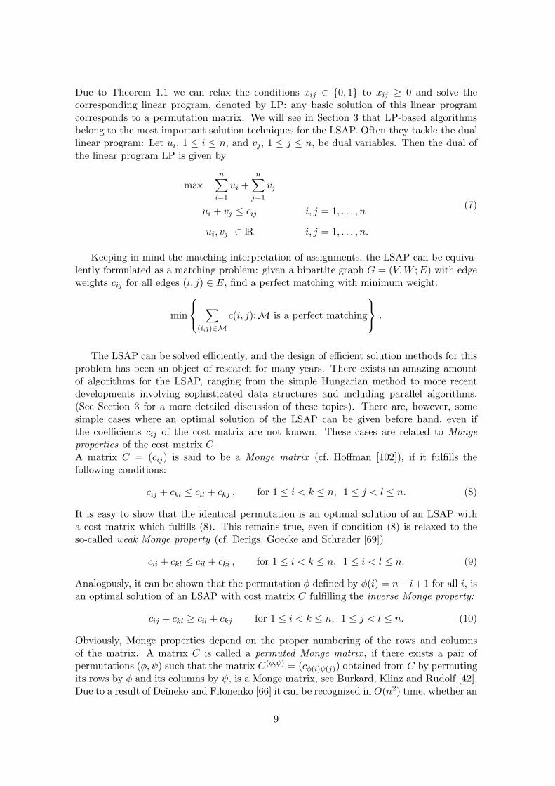
Due to Theorem 1.1 we can relax the conditions xij ∈ {0, 1} to xij ≥ 0 and solve thecorresponding linear program, denoted by LP: any basic solution of this linear programcorresponds to a permutation matrix. We will see in Section 3 that LP-based algorithmsbelong to the most important solution techniques for the LSAP. Often they tackle the duallinear program: Let ui, 1 ≤ i ≤ n, and vj , 1 ≤ j ≤ n, be dual variables. Then the dual ofthe linear program LP is given by

maxn∑

i=1

ui +n∑

j=1

vj

ui + vj ≤ cij i, j = 1, . . . , n

ui, vj ∈ IR i, j = 1, . . . , n.

(7)

Keeping in mind the matching interpretation of assignments, the LSAP can be equiva-lently formulated as a matching problem: given a bipartite graph G = (V,W ;E) with edgeweights cij for all edges (i, j) ∈ E, find a perfect matching with minimum weight:

min

∑

(i,j)∈M

c(i, j):M is a perfect matching

.

The LSAP can be solved efficiently, and the design of efficient solution methods for thisproblem has been an object of research for many years. There exists an amazing amountof algorithms for the LSAP, ranging from the simple Hungarian method to more recentdevelopments involving sophisticated data structures and including parallel algorithms.(See Section 3 for a more detailed discussion of these topics). There are, however, somesimple cases where an optimal solution of the LSAP can be given before hand, even ifthe coefficients cij of the cost matrix are not known. These cases are related to Mongeproperties of the cost matrix C.A matrix C = (cij) is said to be a Monge matrix (cf. Hoffman [102]), if it fulfills thefollowing conditions:

cij + ckl ≤ cil + ckj , for 1 ≤ i < k ≤ n, 1 ≤ j < l ≤ n. (8)

It is easy to show that the identical permutation is an optimal solution of an LSAP witha cost matrix which fulfills (8). This remains true, even if condition (8) is relaxed to theso-called weak Monge property (cf. Derigs, Goecke and Schrader [69])

cii + ckl ≤ cil + cki , for 1 ≤ i < k ≤ n, 1 ≤ i < l ≤ n. (9)

Analogously, it can be shown that the permutation φ defined by φ(i) = n− i+1 for all i, isan optimal solution of an LSAP with cost matrix C fulfilling the inverse Monge property:

cij + ckl ≥ cil + ckj for 1 ≤ i < k ≤ n, 1 ≤ j < l ≤ n. (10)

Obviously, Monge properties depend on the proper numbering of the rows and columnsof the matrix. A matrix C is called a permuted Monge matrix , if there exists a pair ofpermutations (φ,ψ) such that the matrix C(φ,ψ) = (cφ(i)ψ(j)) obtained from C by permutingits rows by φ and its columns by ψ, is a Monge matrix, see Burkard, Klinz and Rudolf [42].Due to a result of Deıneko and Filonenko [66] it can be recognized in O(n2) time, whether an

9

n×n matrix C is a permuted Monge matrix. Moreover, the appropriate permutations φ, ψfor the rows and the columns can also be found within this time bound. As a consequence,the LSAP with a permuted Monge cost matrix can be solved in O(n2) time. The reader isreferred to Burkard et al. [42] for a detailed discussion of Monge properties, and a descriptionof the algorithm of Deıneko and Filonenko.

An important special case of the LSAP with permuted Monge cost matrix arises if the costcoefficients have the form

cij = uivj

with nonnegative numbers ui and vj. Such an LSAP can simply be solved in O(n log n)time by ordering the elements ui and vj.

Theorem 2.1 (Hardy, Littlewood, and Polya [101], 1952)Let 0 ≤ u1 ≤ . . . ≤ un and 0 ≤ v1 ≤ . . . ≤ vn. Then for any permutation φ

n∑

i=1

uivn+1−i ≤n∑

i=1

uivφ(i) ≤n∑

i=1

uivi.

Let us now discuss some applications of the linear sum assignment problem. LSAPsoccur quite frequently as subproblems in more involved applied combinatorial optimizationproblems like the quadratic assignment problem, traveling salesman problems or vehiclerouting problems. Classical direct applications include the assignment of personnel (cf. e.g.Machol [122], Ewashko and Dudding [78]), and the assignment of jobs to parallel machines,but LSAPs have quite a number of further interesting applications. Neng [130] modeled theoptimal engine scheduling in railway systems as an assignment problem. Further applica-tions in the area of vehicle and crew scheduling are described by Carraresi and Gallo [49].

Another application concerns problems in telecommunication, in particular in earth - satel-lite systems. Usually the data to be remitted are buffered in the ground stations and aresent in very short data bursts to the satellite. There they are received by transponders andthen, are transmitted again to the receiving earth station. A transponder just connects onesending station with a receiving station. For a fixed time interval of variable length λk then sending stations are connected with the receiving stations via the n transponders onboardthe satellite, i.e., a certain switch mode is applied. Mathematically, a switch mode Pk cor-responds to a permutation matrix. Then the connections onboard the satellite are changedsimultaneously and in the next time interval new pairs of sending and receiving stationsare connected via transponders, i.e., a new switch mode is applied. Given an (n×n) trafficmatrix T = (tij), where tij describes the amount of information to be remitted from the i-thsending station to the j-th receiving station, we have to determine the switch modes Pk,k = 1, 2, . . ., and the nonnegative lengths λk of the corresponding time slots during whichthe switch modes Pk are applied, such that all data are remitted in the shortest possibletime. Summarizing, our problem consists of finding suited switch modes and correspondinglengths for the time slots during which the switch modes are applied. This leads to thefollowing model:

min∑

kλk

s.t.∑

kλkp

(k)ij ≥ tij , for 1 ≤ i, j ≤ n

λk ≥ 0 , for all k

(11)

10

Since here the time is split among the participating stations, all of them having access tothe satellite, such a traffic model is called time-division-multiple-access (TDMA) model.The problem can be transformed to an LSAP, if a system of 2n fixed switch modesP1, . . . , Pn, Q1, . . . , Qn is installed onboard the satellite, where

∑

k

Pk =∑

l

Ql = 1

and 1 is the matrix with 1-entries only. For details see Burkard [38].

Brogan [37] describes assignment problems in connection with locating objects in space.Let us consider n objects which are detected by two sensors at geographically differentsites. Each sensor measures the angle under which the object can be seen, i.e., it providesn lines, on which the objects lie. The location of every object is found by intersecting theappropriate lines. The pairing of the lines is modeled as follows: let cij be the smallestdistance between the i-th line from sensor 1 and the j-th line from sensor 2. Due tosmall errors during the measurements, cij might even be greater than 0 if some object isdetermined by lines i and j. Solving an LSAP with cost matrix C = (cij) leads to verygood results in practice. A similar technique can be used for tracking n moving objects(e.g. missiles) in space. If their locations at two different times t1 and t2 are known, wecompute the (squared) Euclidean distances between any pair of old and new locations andsolve the corresponding assignment problem in order to match the points in the right way.

For some further applications of assignment problems, including the optimal depletion ofinventory, see Ahuja, Magnanti, Orlin and Reddy [2].

There are also other possibilities for the choice of the objective function in assignmentproblems. For example, if cij is the time needed for machine j to complete job i and all ma-chines run in parallel, the shortest completion time for all jobs is given by max1≤i≤n{ciφ(i)}.This leads to the linear bottleneck assignment problem (LBAP) which will be treated in Sec-tion 5. Other objective functions will be discussed in Section 6.

3 Algorithms for the LSAP

A large number of algorithms, sequential and parallel, have been developed for the linearsum assignment problem (LSAP). They range from primal-dual combinatorial algorithms,to simplex-like methods, cost operation algorithms, forest algorithms, and relaxation ap-proaches. The worst-case complexity of the best sequential algorithms for the LSAP isO(n3), where n is the size of the problem. There is a number of survey papers and bookson algorithms, e.g. Derigs [68], Martello and Toth [126], Bertsekas [30], Akgul [6], and thebook on the first DIMACS challenge edited by Johnson and McGeoch [106]. Among papersreporting on computational experience we mention Derigs [68], Carpaneto, Martello andToth [51], Carpaneto and Toth [56], Lee and Orlin [121], and some of the papers in [106].

Most sequential algorithms for the LSAP can be classified into primal dual algorithmsand simplex-based algorithms. Primal-dual algorithms work with a pair consisting of aninfeasible primal and a feasible dual solution which fulfill the complementarity slacknessconditions. Such algorithms update the solutions iteratively until the primal solution be-comes feasible, while keeping the complementary slackness conditions fulfilled. At this pointthe primal solution is also optimal, according to duality theory.Simplex-based algorithms are special implementations of the primal and the dual simplexalgorithm for linear programming. These algorithms can be applied to solve the LSAP

11

due to Theorem 1.1. Although simplex algorithms are not polynomial in general, there arespecial polynomial implementations of them in the case of the LSAP.More recently, an interior point algorithm has been applied to the LSAP, see Ramakrishnan,Karmarkar, and Kamath [152]. This algorithm produces promising results, in particularwhen applied to large size instances.

From the computational point of view very large scale dense assignment problems withabout 106 nodes can be solved within a couple of minutes by sequential algorithms, see[121].

A number of parallel approaches developed for the LSAP show that the speed upachieved by such algorithms is limited by the sparsity of the cost matrices and/or the de-creasing load across the iterations, see e.g. Balas, Miller, Pekny, and Toth [14], Bertsekas andCastanon [31, 32], Castanon, Smith, and Wilson [53], as well as Wein and Zenios [167, 168].More information on these topics is given in Section 3.4.

3.1 Primal-Dual Algorithms

Primal-dual algorithms work with a pair of an unfeasible primal solution xij , xij ∈ {0, 1},1 ≤ i, j ≤ n, and a feasible dual solution ui, vj , 1 ≤ i, j ≤ n, which fulfill the complementaryslackness conditions:

xij(cij − ui − vj) = 0 , for 1 ≤ i, j ≤ n (12)

We denote cij := cij−ui−vj and call cij reduced costs with respect to the dual solution ui, vj .This pair of solutions is updated iteratively by means of so-called admissible transformationsof the costs matrix C. Also the process of determining the first pair of primal and dualsolutions can be seen as an admissible transformation. A transformation T of a matrixC = (cij) to a matrix C = (cij) is called admissible if for each permutation φ of 1, 2, . . . , nthe following equality holds:

n∑

i=1

ciφ(i) =n∑

i=1

ciφ(i) + z(T ) ,

where z(T ) is a constant which depends only on the transformation T . Clearly, an admis-sible transformation does not change the order of the permutations (feasible solutions ofthe LSAP) with respect to the value of the objective function. Hence the LSAPs with costmatrices C and C are equivalent. We may assume without loss of generality that the entriesof C are nonnegative. (Otherwise we could add a large enough constant to all entries of C.This results in just adding a constant to the objective function, and hence, does not changethe optimal solution of the problem but only its optimal value.)If all entries cij of matrix C are nonnegative and there exists a permutation φ∗ such thatciφ∗(i) = 0, then φ∗ is an optimal solution of the original LSAP with cost matrix C. The

optimal value is equal to z(T ), where T is the transformation from C to C.

Primal-dual algorithms differ on 1) the way they obtain their first pair of a primal and adual solution fulfilling the complementary slackness conditions, and 2) the implementationof the update of dual variables.

The Hungarian method

The first polynomial-time primal-dual algorithm for the LSAP is the Hungarian method dueto Kuhn [118]. In the Hungarian method a starting dual solution is obtained by so-called

12

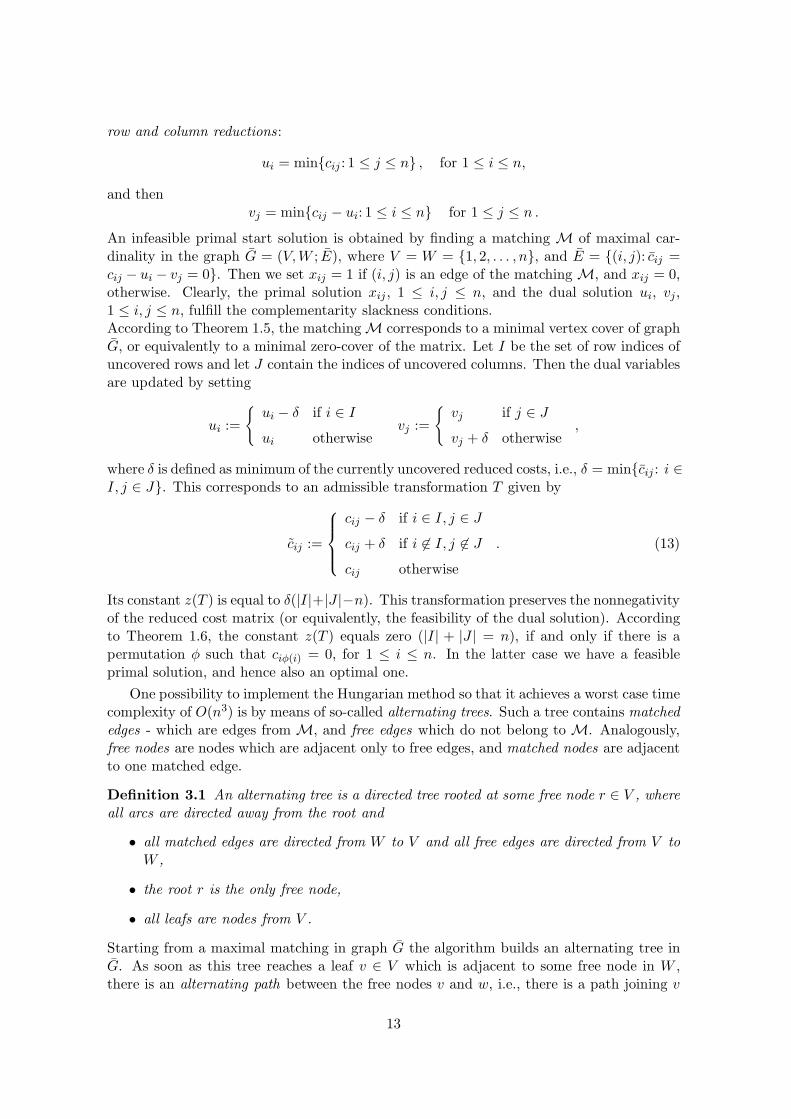
row and column reductions:

ui = min{cij : 1 ≤ j ≤ n} , for 1 ≤ i ≤ n,

and thenvj = min{cij − ui: 1 ≤ i ≤ n} for 1 ≤ j ≤ n .

An infeasible primal start solution is obtained by finding a matching M of maximal car-dinality in the graph G = (V,W ; E), where V = W = {1, 2, . . . , n}, and E = {(i, j): cij =cij − ui − vj = 0}. Then we set xij = 1 if (i, j) is an edge of the matching M, and xij = 0,otherwise. Clearly, the primal solution xij , 1 ≤ i, j ≤ n, and the dual solution ui, vj,1 ≤ i, j ≤ n, fulfill the complementarity slackness conditions.According to Theorem 1.5, the matching M corresponds to a minimal vertex cover of graphG, or equivalently to a minimal zero-cover of the matrix. Let I be the set of row indices ofuncovered rows and let J contain the indices of uncovered columns. Then the dual variablesare updated by setting

ui :=

{

ui − δ if i ∈ I

ui otherwisevj :=

{

vj if j ∈ J

vj + δ otherwise,

where δ is defined as minimum of the currently uncovered reduced costs, i.e., δ = min{cij : i ∈I, j ∈ J}. This corresponds to an admissible transformation T given by

cij :=

cij − δ if i ∈ I, j ∈ J

cij + δ if i 6∈ I, j 6∈ J

cij otherwise

. (13)

Its constant z(T ) is equal to δ(|I|+|J |−n). This transformation preserves the nonnegativityof the reduced cost matrix (or equivalently, the feasibility of the dual solution). Accordingto Theorem 1.6, the constant z(T ) equals zero (|I| + |J | = n), if and only if there is apermutation φ such that ciφ(i) = 0, for 1 ≤ i ≤ n. In the latter case we have a feasibleprimal solution, and hence also an optimal one.

One possibility to implement the Hungarian method so that it achieves a worst case timecomplexity of O(n3) is by means of so-called alternating trees. Such a tree contains matchededges - which are edges from M, and free edges which do not belong to M. Analogously,free nodes are nodes which are adjacent only to free edges, and matched nodes are adjacentto one matched edge.

Definition 3.1 An alternating tree is a directed tree rooted at some free node r ∈ V , whereall arcs are directed away from the root and

• all matched edges are directed from W to V and all free edges are directed from V toW ,

• the root r is the only free node,

• all leafs are nodes from V .

Starting from a maximal matching in graph G the algorithm builds an alternating tree inG. As soon as this tree reaches a leaf v ∈ V which is adjacent to some free node in W ,there is an alternating path between the free nodes v and w, i.e., there is a path joining v

13

and w in G whose edges are alternatively free and matched edges. Such a path is calledan augmenting path, because by exchanging the free and matched edges in it we get a newmaximal matching in G, whose cardinality is larger than that of the previous maximalmatching. In this case we can increase the number of primal variables xij which are equalto 1, and thus improve the primal solution without changing the dual one. There may be atmost n such augmentations because the cardinality of a matching cannot exceed n. Afterhaving performed all possible augmentation steps we get finally a maximal alternating tree,i.e., an alternating tree where all leafs have cardinality equal to 1 in G. At this point, thedual variables - and with them the reduced costs and the graph G - are updated by anadmissible transformation. Thus some new edges are added to G, i.e., additional reducedcosts equal to 0 arise. Now the existing alternating tree can be updated with respectto the new graph G. It is possible to implement the update of dual variables so thatall due updates between two consecutive augmentations are performed by applying O(n2)elementary operations. Since there may be at most n augmentations, this leads to an O(n3)algorithm.

Shortest augmenting path algorithms

Although the Hungarian algorithm described above grows an alternating tree to augmentthe primal solution, in principle only alternating augmenting paths are used. This observa-tion is the conceptual basis of numerous shortest augmenting path algorithms for the LSAP,which belong to the class of primal-dual methods and can also be implemented in O(n3)steps. Given a pair of a primal solution xij, 1 ≤ i, j ≤ n, and a dual feasible solutionui, vj , 1 ≤ i, j ≤ n, which fulfill the complementarity slackness conditions, together withthe reduced costs cij , construct a weighted directed bipartite graph G = (V,W ; E) witharc set E = D ∪ R. Here D = {(i, j): (i, j) ∈ E, xij = 0} is the set of forward arcs, andR = {(j, i): (i, j) ∈ E, xij = 1} is the set of backward arcs. The weights of the backwardarcs are set equal to 0, whereas the weights of the forward arcs are set equal to the corre-sponding reduced costs. We select a free node r in V and solve the single-source shortestpath problem, i.e., compute the shortest paths from r to all nodes of G. The shortest amongall paths from r to some free node in W is used to augment the current primal solution byswapping the free and matched edges. The primal and dual solutions as well as the reducedcosts are updated similarly as in the case of the Hungarian method. It can be shown thateach (unfeasible) primal solution (or equivalently, each matching in G) constructed in thecourse of the algorithm has minimum weight among all solutions of the same cardinality, seee.g. Lawler [119], Derigs [68]. Hence, after n augmentations we obtain an optimal primalsolution. The single-source shortest paths can be computed in O(n2) time in a graph withnonnegative weights, e.g. by applying the Dijkstra algorithm implemented with Fibonacciheaps, see Fredman and Tarjan [80]. This implies that the overall complexity of augmentingpath algorithms amounts to O(n3).

The shortest path computation may stop as soon as the first path joining r with some freenode in W has been computed.

Basically shortest augmenting path algorithms for the LSAP may differ in the way theydetermine a starting pair of primal and dual solutions, and by the subroutine they usefor computing the shortest paths. (The reader is referred to Cherkassky, Goldberg, andRadzik [59] for a review on shortest paths algorithms. For developments on data structuresused in shortest path algorithms the reader is referred to Fredman and Tarjan [80], and toAhuja, Mehlhorn, Orlin, and Tarjan [3].) Most of the existing algorithms use the Dijkstra

14

algorithm for the shortest path computations, e.g. Carpaneto and Toth [56], Jonker andVolgenant [107, 108], and Volgenant [164].Several authors try to speed up the shortest path computations by thinning out the un-derlying bipartite graph, e.g. Carraresi and Sodini [52], Glover, Glover, and Klingman [90].In these algorithms only “short” edges of the graph G are considered in the shortest pathcomputations. A threshold value which is updated after each augmentation is used to deter-mine the short edges. Therefore these algorithms are sometimes called threshold algorithms.Their worst case complexity is also O(n3).Some shortest augmenting path algorithms apply specific implementations of shortest pathscomputations especially suited for sparse matrices, see [56], and [164]. To apply this tech-nique the cost matrix is thinned-out by some heuristic. If no feasible primal solution isfound for the sparse problem, then the cost matrix is enlarged by re-adding some of the“canceled” entries.

The auction algorithm

Another primal-dual algorithm, called the auction algorithm, has been proposed by Bert-sekas [28]. The auction algorithm is similar to the Hungarian method to the extent that theupdates of primal and dual solutions can be modeled by admissible transformations. How-ever, whereas in the Hungarian method the value of the dual objective function increasesafter each such an update, in auction algorithms it is only guaranteed that this value doesnot decrease. Another difference is that in the Hungarian algorithm a matched vertex ofV or W remains matched for the rest of the algorithm, while this property only holds forvertices of V in the case of the auction algorithm. Some vertex of W matched in a certainiteration of the auction algorithm may become free in some further iteration. The originalauction algorithm was developed for maximization problems, where we try to maximizethe objective function of the LSAP under the assignment constraints. In the minimizationcase the auction algorithm associates each vertex of W with an item to be sold, and eachvertex of V with a customer. cij is the cost of item j for customer i, the dual variable vjis the profit on item j, and the difference cij − vj is customer’s i cost margin relative tothe profit on item j. The algorithm starts with a pair of an (unfeasible) primal solution xij(e.g. xij = 0 for all i, j) and a feasible dual solution ui, vj . This pair of solutions fulfills thecomplementarity slackness conditions (12), and is updated iteratively by maintaining (12).The update of the current xij , ui, vj , to obtain the subsequent pair of solutions x′ij , u

′i, v

′j,

is made by choosing a free customer i (i ∈ V ), and by determining the smallest and secondsmallest cost margin u and u, respectively:

u = min{cij − vj: 1 ≤ j ≤ n} , j = argmin{cij − vj : 1 ≤ j ≤ n} ,

u = min{cij − vj : 1 ≤ j ≤ n, j 6= j} .Then the algorithm distinguishes two cases: Case 1, where u < u, or u = u and j is free,and Case 2, where u = u and j is matched. In the first case the algorithm assigns i to j(x′ij

= 1) and updates the dual variables ui and vj so as to preserve dual feasibility: u′i= u

and v′j

= vj + (u− u). If j was not a free vertex, i.e., there was some i such that xij = 1,

the new primal solution sets x′ij

= 0. In the second case, where u = u and there is an index

i such that xij = 1, the algorithm sets ui := u and performs a labeling procedure to either

update the dual variables so as to assign j to i or to get an augmenting path starting from iand ending at some free vertex in W . In the latter case we would have an update of the pair

15

of primal and dual solutions as in the case of the Hungarian method (see [28] for a completedescription). This auction algorithm is pseudopolynomial and runs in O(n2(n + R)) time,where R = max{|cij |: 1 ≤ i, j ≤ n}. The similarity with the Hungarian method allowsthe combination of both algorithms as proposed in [28]. The combined algorithm starts byapplying the auction algorithm, counts the iterations which do not lead to an increase ofthe number of items assigned to customers, and switches to the Hungarian method as soonas the counter exceeds an appropriately defined parameter. It can be shown that the worstcase complexity of this combination is O(n3).

Bertsekas and Eckstein [35] modified the above described auction algorithm to obtain apolynomial-time algorithm with worst case complexity O(n3 log(nR)), where R is definedas above. The algorithm works with a pair of a primal and a dual solution which fulfillsthe ǫ-complementarity conditions

xij(cij − ui − vj) ≥ −ǫ , for 1 ≤ i, j ≤ n.

In terms of the ǫ-complementarity conditions an ǫ-relaxed problem is defined: It consistsof finding a pair of feasible primal and dual solutions of the given LSAP which fulfills theǫ-complementarity conditions. It can be shown that an optimal solution of the 1/n-relaxedproblem (ǫ = 1

n) is also an optimal solution of the initial problem. This fact suggests toapply so-called scaling techniques, i.e., to solve initially the ǫ-relaxed problem for a large ǫ,and then to decrease ǫ gradually until it reaches 1/n.

When ǫ is decreased to ǫ′ the optimal solution of the previous ǫ-relaxed problem is updatedwith “few” efforts to obtain the optimal solution of the ǫ′-relaxed problem. Bertsekas et al.[35] implement this ǫ-scaling in terms of a scaling of the costs. All costs cij are multipliedby n + 1 and a 1-relaxed problem (ǫ = 1) is solved. If xij and ui, vj are optimal primaland dual solutions of the 1-relaxed problem with costs c′ij = (n + 1)cij , then xij and ui

n+1 ,vj

n+1 , is an optimal pair of primal and dual solutions for the 1n -relaxed problem with costs

cij . Consequently, xij is an optimal solution of the LSAP with costs cij . The 1-relaxedsubproblem with costs c′ij is solved by solving M = O(log(nR)) subproblems consecutively.

The m-th subproblem is a 1-relaxed LSAP with costs given byc′ij

2M−m , and is solved by analgorithm similar to the original auction algorithm [28]. For a free node i ∈ V , the valuesu, u, and the index j ∈ W are determined as in the original auction algorithm, and twoanalogous cases are distinguished. The dual variable corresponding to i is set to ui := u+ ǫ

2 ,and the dual variable corresponding to j is set to vj := vj + (u− u) − ǫ

2 .

Bertsekas et al. [35] call bidding the update of ui. The version where one node bids at a timeis called Gauss–Seidel version of the auction algorithm and is better suited for sequentialimplementations (see [35] for more information). Another version, where all free customersbid simultaneously is called Jacobi version of the auction algorithm and is more appropriatefor parallel implementations, see Bertsekas [29].

Pseudoflow algorithms

Other primal-dual algorithms for the LSAP are based on the formulation of the LSAPas a minimum cost flow problem (see Section 1). A pseudoflow is a flow which fulfills thecapacity constraints (3), but does not necessarily fulfill the flow conservation constraints (2).Pseudoflow algorithms work with ǫ-relaxations of the minimum cost flow problem wherethe flow conservation constraints are violated by at most ǫ. They iteratively transformthe starting solution, which is a pseudoflow, into an optimal solution for the ǫ-relaxed

16

problem. Then, ǫ is decreased and the procedure is repeated until ǫ reaches 1n . At that

point an optimal solution of the ǫ-relaxed flow problem is also an optimal solution forthe original flow problem, and hence for the LSAP. The general idea is quite similar to theauction algorithm of Bertsekas et al. [35] which involves ǫ-complementarity conditions. Onedifference is that pseudoflow algorithms apply ǫ scaling, whereas the auction algorithm in[35] applies cost scaling. Another difference concerns the transformation of a pseudoflowinto an optimal solution of the ǫ-relaxed flow problem, which is done by the push-relabelmethod described by different authors, e.g. Goldberg and Tarjan [96], Cherkassky andGoldberg [58]. If ǫ is divided by δ ≥ 2 in each iteration, it can be shown that the pushrelabel algorithm terminates after O(logδ(nR)) iterations, where R is defined as in theprevious section. Different pseudoflow algorithms for the LSAP have been developed byOrlin and Ahuja [133], Goldberg, Plotkin and Vaidya [95], and Goldberg and Kennedy [94].These algorithms are particularly efficient for sparse problems: the worst-case complexity ofthe first two algorithms is O(

√nm log(nR)), where m is the number of finite entries of the

cost matrix C. (Infinite entries correspond to non-existing edges in the matching model.)

3.2 Simplex-Based Algorithms

Simplex-based algorithms for the LSAP are specific implementations of the network simplexalgorithm. The latter is a specialization of the simplex method for linear programming tonetwork problems and is due to Dantzig, see e.g. [65]. The specialization relies on exploitingthe combinatorial structure of network problems to perform more efficient pivots acting ontrees rather than on the coefficient matrix. A number of such algorithms for the LSAP,and more generally for the transportation problem of whom the LSAP is a special case,have been developed in the early 1970s, see e.g. Glover, Karney and Klingman [91], Gloverand Klingman [92]. It is well known that there is a one-to-one correspondence betweenprimal (integer) basic solutions of the LSAP and spanning trees of the bipartite graph Grelated to assignment problems as described in Section 1. Moreover, given the spanningtree, the values of the corresponding dual variables fulfilling the complementarity slacknessconditions are uniquely determined, as soon as the value of one of those variables is fixed(arbitrarily). Every primal feasible basic solution is highly degenerate because it contains2n − 1 variables and n − 1 of them are equal to 0. Hence degeneracy poses a problem,and the first simplex-based algorithms for the LSAP were exponential. The first stepstowards the design of polynomial-time simplex-based algorithms were made by introducingthe concept of so-called strongly feasible trees, due to Cunningham [62, 63] and Barr, Glover,and Klingman [26].

Primal simplex-based algorithms

Primal simplex-based algorithms work with a primal feasible basic solution which corre-sponds to a spanning tree T in G. n of the x variables corresponding to edges of the treeare equal to 1, the other n− 1 edges of the tree correspond to x variables equal to 0. Giventhe primal variables xij , the dual variables ui, vj are uniquely determined by setting one ofthem arbitrarily and computing the others such that the complementarity conditions arefulfilled, i.e., cij = cij − ui − vj = 0 for all i, j such that (i, j) ∈ T . If the reduced costscorresponding to the edges of the co-tree T c = E \ T are nonnegative, the current basis Tis optimal. Otherwise, there is an edge (i, j) = e ∈ TC with cij < 0. Adding this edge to Tcreates a unique cycle C(T, e). The subsequent basis T ′ is given by T ′ := (T \ {f}) ∪ {e},where f = (i′, j′) is some edge in C(T, e), with xi′j′ = min{xij : (i, j) ∈ C(T, e)}.

17

Barr et al. [26] and Cunningham [62, 63] introduced a special type of spanning trees in G,called strongly feasible trees. They showed that the network simplex method for the LSAPcan be implemented so as to visit only bases which correspond to strongly feasible trees.Strongly feasible trees are defined similarly as alternating trees in the Hungarian method.

Definition 3.2 A strongly feasible tree is a rooted directed tree in G with root in V andarcs directed away from the root, such that for all arcs (i, j) with i ∈ V and j ∈W , xij = 1,and for all arcs (i, j) with i ∈W and j ∈ V , xij = 0.

Strongly feasible trees have a number of useful properties with respect to the primal networksimplex algorithm. Before we describe them, let us say that (i, j) = f ∈ TC is a forward(backward) arc if i ∈ V (j ∈W ) lies on the directed path joining the root r of T with j ∈W(i ∈ V ). An arc f which is neither backward nor forward is called a cross arc.

Proposition 3.3 (Barr et al. [26], 1977, Cunningham [62, 63], 1976, 1979) Let T be astrongly feasible tree for an LSAP instance, and let TC be its corresponding co-tree. Then

1. The root has degree 1, every other node from V has degree 2.

2. If the edges e = (i, j) and f = (i′, j′), i, i′ ∈ V , j, j′ ∈ W , satisfy the propertiese ∈ TC, f ∈ c(T, e), and i ≡ i′ then (T \ {f}) ∪ {e} is again a strongly feasible tree.

3. For an e ∈ TC the pivot by the pair (e, f) defined as above is non-degenerate iff e isa forward arc.

Cunningham showed that the primal network simplex algorithm for the LSAP cannot per-form more than O(n2) degenerate pivots at some vertex of the assignment polytope, ifstrongly feasible trees and a specific pivot rule are employed. By combining these ideaswith Dantzig’s pivot rule (the new basic variable is that with the most negative reducedcost), Hung [104] obtained an algorithm which performs at most O(n3log∆) pivots, where∆ is the difference between the objective function value of the starting solution with theoptimal one. Orlin [132] reduced the number of pivots to O(n3 log n) for the primal net-work simplex algorithm with Dantzig’s rule. He exploits the fact that employing stronglyfeasible trees is equivalent to running the standard network simplex algorithm with somelexicographic pivoting rule for an appropriately perturbed problem. (This fact was alsoobserved by Cunningham [62].) By scaling the coefficients of the perturbed problem, anupper bound of O(n2 log ∆) on the number of pivots is obtained. In the case of LSAPs canbe shown that there exists an equivalent problem with cost coefficients bounded by 4n(n!)2,and hence ∆ = O(n log n).

Another primal simplex algorithm which uses a pivot rule similar to Dantzig’s was proposedby Ahuja and Orlin [4]. Assuming that the cost coefficients are integral, the algorithmperforms at most O(n2 logR) pivots and has a worst case complexity of O(n3 logR), whereR is defined as R = max{|cij |: 1 ≤ i, j ≤ n}. The pivot rule involves scaling, and a pivotedge is chosen among those edges (i, j) for which cij ≤ −0.5ǫ. If at any stage in thealgorithm there does not exist a pair (i, j) which fulfills cij ≤ −0.5ǫ, then ǫ is divided by 2.This process is continued until ǫ becomes less than 1. At this point an optimal solution isreached.

Based on strongly feasible trees Roohy-Laleh [154] gave a strongly polynomial primalnetwork-simplex algorithm which performs at most O(n3) pivots and has a worst-case com-plexity of O(n5).

18

Akgul [7] designed a primal simplex algorithm which performs O(n2) pivots and has anoverall worst case complexity of O(n3). Also this algorithm uses strongly feasible trees asbasic solutions and Dantzig’s pivot rule to choose the variable which enters the basis. Aspecial feature of the algorithm is that it solves an increasing sequence of LSAPs whichare subproblems of the original one, in the sense that the edge sets of the correspondinggraphs are subsets of the edge set E for the original problem. The edge set associated witha certain subproblem is obtained by adding some edges incident to a single node to theedge set associated with the previous subproblem. The last subproblem in the sequenceis the original LSAP. The author investigates the structure and properties of so-called cutsets which are sets of vertices whose dual variables are changed during the solution of asubproblem. It can be shown that the cut sets are disjoint, and that edges whose heads liein the cut set are dual feasible for all subgraphs considered afterwards. By exploiting theseproperties it is shown that the optimal solution of the (i+1)-st subproblem can be found byperforming at most k + 2 pivots starting from an optimal solution of the i-th subproblem.

Dual simplex-based algorithms

A spanning tree T of the graph G, besides determining uniquely an integer valued basicsolution for the LSAP, determines also a basic solution of the dual (7) of the LSAP. Thisis done by setting the value of one of the variables arbitrarily, say u1 = 0, and the othervariables so as to fulfill ui + vj = cij for all i, j such that (i, j) ∈ T . This dual solution isunique up to the arbitrary setting of one of the variables. Moreover, this basic dual solutionis feasible iff cij = cij − ui − vj ≥ 0. Clearly, if both primal and dual solutions determinedby T are feasible, then both of them are optimal.

Dual simplex methods for the LSAP work with a tree T which defines a dual feasible basicsolution and keep transforming T iteratively until the corresponding primal solution isfeasible, and hence, optimal. The transformation is done by pivoting on an edge e = (k, l)of E \ T for which the corresponding primal constraint is violated, i.e., xkl ≤ −1. Thisedge is added to the current tree T and one of the edges, say f , contained in the cycleC(T, e) is removed from T to form a new tree T ′ = (T \ {f}) ∪ {e}. In order to keep dualfeasibility the chosen edge f = (i, j) should fulfill i ∈ T (k), j ∈ T (l), where T (k), T (l) are thesubtrees of T which arise when the edge e = (k, l) is removed from T , and contain k and l,respectively.

Different rules for the choice of the edges e and f yield different dual simplex algorithms.Many of these algorithms make use of so-called signatures, introduced by Balinski [18].Therefore, such algorithms are also called signature methods.

Definition 3.4 Consider an LSAP and a spanning tree T in the graph G = (V,W ;E)related to the LSAP. The row (column) signature of T is the vector of the degrees in T ofthe vertices in V (W ) for some arbitrary but fixed order of those vertices.

It can be shown that a spanning tree T which defines a dual feasible basis and whoserow signature contains only one 1 and the other entries equal to 2 is an optimal basis.Consequently, the primal solution defined as follows is optimal. Start with xkl=1 for k ∈ Vbeing the node of degree 1 and (k, l) ∈ T . Set the other variables xij such that theassignment constraints are fulfilled and xij = 0 for (i, j) 6∈ T . Thus the LSAP is reducedto finding a dual feasible tree with row (column) signature (1, 2, 2, . . . , 2). Balinski [18, 19]proposes two algorithms to find such a tree T . Both algorithms start with a tree withrow signature (n, 1, . . . , 1) and dual variables u1 = 0, vj = c1j for 1 ≤ j ≤ n, and ui =

19

minj{cij − vj}, for 2 ≤ i ≤ n. Such a tree is often called a Balinski tree. In the firstalgorithm [18] the choice of the pivoting edges e and f is guided only by the signatures,trying to decrease the number of 1-s in the signature. This makes the algorithm a non-genuine simplex method because it may pivot on some edge e = (k, l) with xkl = 0.Moreover, the algorithm does not stop when an optimal solution with signature differentfrom (1, 2, . . . , 2) is found. The algorithm performs at most O(n2) operations to decreasethe number of 1-s in the signature by 1. Hence its worst case complexity is O(n3).

Goldfarb [97] proposed a similar algorithm based on signatures which solves a sequenceof subproblems of the given LSAP. As in the algorithm of Akgul [7] the subproblems areLSAPs with cost matrices being submatrices of C = (cij). The cost matrix of the k-thsubproblem is defined by the first k rows and the first k columns of C. Balinski’s algorithmis used to solve the k-th subproblem, i.e., to produce a tree corresponding to a dual feasiblebasis with signature (2, . . . , 2, 1). After the transition to the (k + 1)-st subproblem, i.e.,after the introduction of the (k + 1)-st row and column of matrix C, the signature eitherremains optimal or has the form (3, 2, . . . , 2, 1, 1). In the latter case at most k − 1 pivotsare needed to produce a tree with signature (2, . . . , 2, 1) for the (k+1)-st problem. Clearly,this algorithm is not a genuine simplex dual algorithm for the same reasons as Balinski’salgorithm.

The second algorithm of Balinski [19] employs another pivot rule which is a combination ofthe rule based on signatures used in [18] and the classical pivot on an edge e = (i, j) withthe most negative xij. This rule allows the algorithm to visit only so-called strongly dualfeasible trees. These trees are defined in terms of so-called odd and even arcs. Consider atree T corresponding to a dual feasible solution and root it at the first vertex in V (accordingto some fixed arbitrary order) and direct all edges away from the root. An arc (i, j) ∈ Twith i ∈ V , j ∈ W , is called odd arc and an arc (j, i) with j ∈ W and i ∈ V is called evenarc. A dual feasible tree is strongly dual feasible if xij ≥ 1 for all even arcs (i, j) ∈ T , andxij ≤ 0 for all odd arcs (i, j) ∈ T which do not join 1 = i ∈ V with a node j of degree 1in W . The algorithm proposed in [19] pivots only on edges (i, j) for which xij < 0. Hence,this algorithm is a genuine dual simplex method, sometimes also called competitive simplexalgorithm. The number of pivots is at most (n − 1)(n − 2)/2, thus yielding a worst casetime complexity of O(n3).

Kleinschmidt, Lee, and Schannath [114] have shown that this algorithm of Balinski [19] isequivalent to an algorithm proposed earlier by Hung and Rom [105].

Akgul [5] proposed an algorithm similar to Goldfarb’s. The two main differences are:1) Akgul’s algorithm works with strongly dual feasible trees, i.e., it finds a strongly dualfeasible tree for the k-th problem and transforms it into a strongly dual feasible tree forthe (k + 1)-st problem, and 2) the subproblems considered by Akgul are transportationproblems. The algorithm performs at most O(n2) pivots and has a worst case complexityof O(n4).

A similar algorithm was developed by Paparrizos [136]. The main difference to Akgul’salgorithm is that here the subproblems are determined with the help of a Balinski tree.They are, however, solved in the same way as in [5].

Two other signature-guided algorithms were given by Paparrizos [135] and Akgul andEkin [8]. Paparrizos’ algorithm is similar to Balinski’s competitive simplex algorithm [19].The main difference concerns the dual feasibility which is not an invariant of Paparrizos’algorithm. The algorithm starts with a Balinski tree. Then it performs pivots whichmay produce infeasible dual solutions. The pivots are grouped in stages and each stage

20

starts (and stops) with a strongly dual feasible tree. The last tree of the last stage isalso primal feasible and hence optimal. The algorithm visits only so-called strong treeswhich are obtained from strongly feasible trees by dropping the feasibility requirement.The algorithm performs O(n2) pivots but spends as much time to determine the pair ofedges involved in a pivot. Thus the overall complexity is O(n4). Akgul and Ekin [8] givean efficient implementation of Paparrizos’ algorithm, which maintains and updates a forestrather than a single tree. In this way only dual feasible trees are visited. The number ofpivots is again O(n2) but the overall complexity becomes O(n3).

Later, Paparrizos [137] designed a purely infeasible simplex algorithm which performs O(n2)pivots and has worst case complexity of O(n3). This algorithm is similar to the algorithmpresented in [135] since it starts again with a Balinski tree and visits only strong trees.Also the edge inserted to a the current strong tree during a pivot operation is determinedas in [135]. The edge which is removed from the tree is determined, however, by a differentrule. In contrast with the previous algorithm proposed in [135], this algorithm is purelyinfeasible in the sense that it restores dual feasibility only when it stops with an optimalsolution.

3.3 Other Algorithms

A primal algorithm of Balinski and Gomory [20]

The algorithm of Balinski and Gomory is probably the oldest primal algorithm for theLSAP. It works with a perfect matching M in the graph G (i.e., a primal feasible solutionxij, 1 ≤ i, j ≤ n) and dual variables ui, vj , 1 ≤ i, j ≤ n, which fulfill the complementaryslackness conditions. The primal and dual solutions are updated iteratively by maintainingthereby the complementarity slackness conditions. Let E = {(i, j): cij = cij − ui − vj ≥ 0}.If E = E than the primal solution M and the dual solution ui, vj , 1 ≤ i, j ≤ n, are optimal.If there is an edge e = (i, j) 6∈ E, then there exists an edge (r, j) ∈ M. The algorithm buildsan alternating tree T in the subgraph (V,W ; E) of G and grows it by updating the dualvariables similarly as in the primal-dual methods. Then, the matching is changed if thereis a cycle in T ∪ {e}. This procedure is repeated until E = E. A characteristic feature ofthe algorithm is that E grows monotonically in the course of the algorithm, i.e., if an edgebecomes dual feasible at a certain iteration it remains feasible in the subsequent iterationsuntil the algorithm stops. An efficient version of this algorithm with time complexity O(n3)has been described by Cunningham and Marsh [64].

Cost Operator Algorithms

Two other primal algorithms for the transportation problem, and hence also for the LSAP,are the cost operator algorithms developed by Srinivasan and Thompson [158]. In contrastto the algorithm of Balinski and Gomory these algorithms work with primal basic solutions.Both algorithms start with a dual feasible solution ui, vj , 1 ≤ i, j ≤ n, found by the usualrow/column reductions: compute the column minima, subtract them from the columns,then compute the row minima and subtract them from the rows. Then both algorithmsconstruct a primal feasible basic solution xij (xij are reals between 0 and 1), and introducenew costs: cij = ui + vj for all i, j such that xij is in the basic solution, and cij = cij ,otherwise. Thus, xij and ui, vj form a pair of feasible primal and dual solutions for theLSAP with cost matrix (cij). This pair of solutions fulfills the complementarity slacknessconditions. Hence both solutions are optimal. Next both algorithms change step by step

21

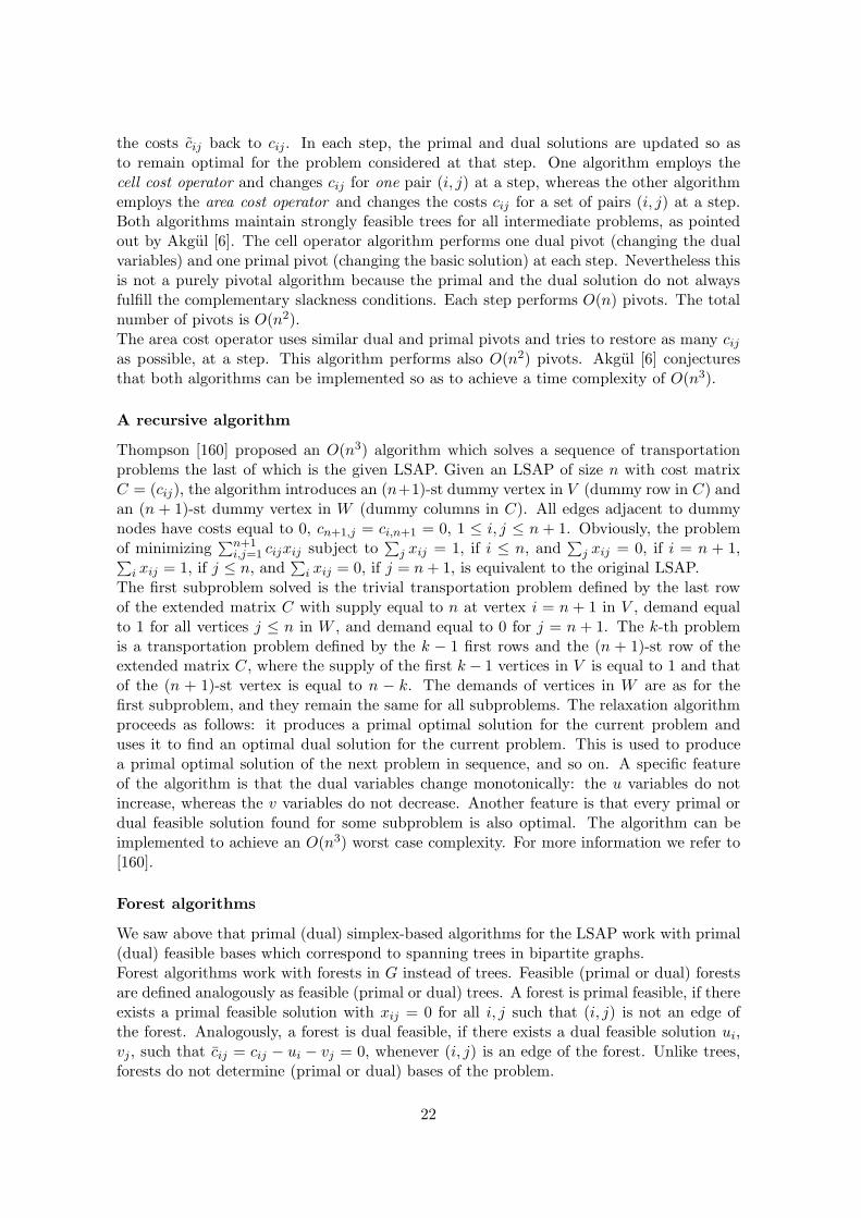
the costs cij back to cij. In each step, the primal and dual solutions are updated so asto remain optimal for the problem considered at that step. One algorithm employs thecell cost operator and changes cij for one pair (i, j) at a step, whereas the other algorithmemploys the area cost operator and changes the costs cij for a set of pairs (i, j) at a step.Both algorithms maintain strongly feasible trees for all intermediate problems, as pointedout by Akgul [6]. The cell operator algorithm performs one dual pivot (changing the dualvariables) and one primal pivot (changing the basic solution) at each step. Nevertheless thisis not a purely pivotal algorithm because the primal and the dual solution do not alwaysfulfill the complementary slackness conditions. Each step performs O(n) pivots. The totalnumber of pivots is O(n2).The area cost operator uses similar dual and primal pivots and tries to restore as many cijas possible, at a step. This algorithm performs also O(n2) pivots. Akgul [6] conjecturesthat both algorithms can be implemented so as to achieve a time complexity of O(n3).

A recursive algorithm

Thompson [160] proposed an O(n3) algorithm which solves a sequence of transportationproblems the last of which is the given LSAP. Given an LSAP of size n with cost matrixC = (cij), the algorithm introduces an (n+1)-st dummy vertex in V (dummy row in C) andan (n + 1)-st dummy vertex in W (dummy columns in C). All edges adjacent to dummynodes have costs equal to 0, cn+1,j = ci,n+1 = 0, 1 ≤ i, j ≤ n + 1. Obviously, the problemof minimizing

∑n+1i,j=1 cijxij subject to

∑

j xij = 1, if i ≤ n, and∑

j xij = 0, if i = n + 1,∑

i xij = 1, if j ≤ n, and∑

i xij = 0, if j = n+ 1, is equivalent to the original LSAP.The first subproblem solved is the trivial transportation problem defined by the last rowof the extended matrix C with supply equal to n at vertex i = n + 1 in V , demand equalto 1 for all vertices j ≤ n in W , and demand equal to 0 for j = n + 1. The k-th problemis a transportation problem defined by the k − 1 first rows and the (n + 1)-st row of theextended matrix C, where the supply of the first k − 1 vertices in V is equal to 1 and thatof the (n + 1)-st vertex is equal to n − k. The demands of vertices in W are as for thefirst subproblem, and they remain the same for all subproblems. The relaxation algorithmproceeds as follows: it produces a primal optimal solution for the current problem anduses it to find an optimal dual solution for the current problem. This is used to producea primal optimal solution of the next problem in sequence, and so on. A specific featureof the algorithm is that the dual variables change monotonically: the u variables do notincrease, whereas the v variables do not decrease. Another feature is that every primal ordual feasible solution found for some subproblem is also optimal. The algorithm can beimplemented to achieve an O(n3) worst case complexity. For more information we refer to[160].

Forest algorithms

We saw above that primal (dual) simplex-based algorithms for the LSAP work with primal(dual) feasible bases which correspond to spanning trees in bipartite graphs.Forest algorithms work with forests in G instead of trees. Feasible (primal or dual) forestsare defined analogously as feasible (primal or dual) trees. A forest is primal feasible, if thereexists a primal feasible solution with xij = 0 for all i, j such that (i, j) is not an edge ofthe forest. Analogously, a forest is dual feasible, if there exists a dual feasible solution ui,vj, such that cij = cij − ui − vj = 0, whenever (i, j) is an edge of the forest. Unlike trees,forests do not determine (primal or dual) bases of the problem.

22

A primal-dual forest algorithm, or more precisely a forest implementation of the Hungarianmethod, has been described by Akgul in [6]. The algorithm iteratively solves a shortestpath problem in the graph G associated with the assignment problem, and equipped withthe reduced costs cij as edge lengths. This is done by growing a forest of alternating treesrooted at a free node in V each and by exploiting the relationship between alternatingtrees and strongly feasible trees. As soon as the leafs of an alternating tree are joined byedges with free nodes in W , a strongly feasible tree arises. The algorithm maintains a setof alternating trees called planted forest , and a set of strongly feasible trees called matchedforest. Each augmentation transforms an alternating tree in a strongly feasible tree, untilthe planted forest becomes empty. The augmentations employ labeling and update of dualvariables like all primal-dual algorithms in general, and the Hungarian method in particular.

An O(n3) forest algorithm is proposed by Achatz, Kleinschmidt, and Paparrizos [1] and isa more efficient variant of the algorithm proposed by Paparrizos in [137]. The algorithmstarts with some basic dual feasible tree rooted at some arbitrary node in V , and constructsa forest by deleting all edges (i, j) where i ∈ V , j ∈W , and i is the father of j with respectto the usual orientation of the tree which directs all edges away from the root. This yieldsa spanning forest which is dual feasible. All nodes in W are considered as roots of theconnected components to which they belong. Further, the algorithm works with superforestswhich are forests where every connected component contains one root, and nodes from W ,which are not roots, have degree equal to 2. The starting forest constructed as above isa superforest . Each superforest is divided into a surplus forest and a deficit forest. Thesurplus forest contains all connected components whose roots have degree larger than 1.The deficit forest is the complement of the surplus forest with respect to the consideredsuperforest. The algorithm constructs a sequence of dual feasible superforests by applyinga special pivoting strategy. It stops when a superforest with an empty surplus forest isfound. It can be shown that this yields a dual optimal solution of the considered LSAP.

3.4 On Parallel Algorithms

Since the late 1980s a number of parallel algorithms for the LSAP has been proposed. Theyare parallelized versions of primal-dual algorithms based on shortest path computations, dueto Kennington and Wang [113], Zaki [170], Balas, Miller, Pekny, and Toth [14], Bertsekasand Castanon [32, 33], parallelized versions of the auction algorithm, due to Zaki [170],Wein and Zenios [167, 168], Bertsekas and Castanon [31], and parallelizations of primalsimplex-based methods, due to Miller, Pekny, and Thompson [128], Peters [138], Barr andHickman [27]. For a good review on parallel algorithms for the LSAP and network flowproblems in general the reader is referred to Bertsekas, Castanon, Eckstein, and Zenios [34].

Parallel implementations of primal-dual shortest path algorithms

The primal-dual parallel algorithms based on shortest path computations can be classifiedinto single node algorithms and multi-node algorithms. Single node algorithms compute ashortest path tree from a single free source node in parallel, i.e., by parallelly scanning thearcs connected to a single node. Most of these algorithms are obtained as implementations ofthe algorithm of Jonker and Volgenant [107]. As shown in [113, 170], considerable speedupscan be obtained in the case of dense assignment problems. Kennington et al. [113] obtaina speedup of 3–4 for a number of processors between 3 and 8. For sparse problems the

23

speedups decrease, since the amount of work which can be performed in parallel decreases.Thus, the effectiveness of these algorithms is limited by the density of the input network.Computational results, e.g. Castanon, Smith, and Wilson [53], show that single instructionstream multiple data stream (SIMD) shared memory massively parallel architectures arewell suited for implementing single node parallel algorithms to solve dense problems.

Multi-node approaches compute multiple augmenting paths starting from different freenodes, and perform multiple augmentations and updates of variables in parallel. Balas etal. [14] propose a synchronous algorithm of this type which employs a coordination protocolto combine all augmentations and changes of the dual variables so as to maintain feasibilityand keep the complementarity slackness conditions fulfilled. Bertsekas et al. [32] extendthis protocol to obtain asynchronous algorithms. The coordination in the asynchronousalgorithm is realized by maintaining a master copy of a pair of primal and dual solutionswhich can be accessed by all processors. The latter compute augmenting paths and variableupdates based on the copy of the primal and dual solution they have, and then checkwhether the update is feasible (the master copy may have been updated in the meanwhile).If the update is feasible, the master copy is updated. The master copy is locked duringthe updates. Computational experience with these algorithms shows that their principallimitation is the decreasing amount of parallel work with the number of iterations. Initiallymany augmenting paths can be found so that many processors can be used effectively. Thenthe load decreases as the number of iterations increases. When comparing synchronousand asynchronous implementations Bertsekas et al. [32] show that for sparse problemsasynchronous algorithms may be outperformed by synchronous algorithms. This is basicallydue to the considerable coordination overhead of the asynchronous algorithms.

Parallel implementations of the auction algorithm

Recall that the auction algorithm computes in each iteration the smallest and the secondsmallest cost margin with respect to the profit for each free customer. Different implemen-tations may compute these differences (also called bids in the maximization version of theLSAP) for all free customers - resulting in the so-called Jacobi methods, for a single freecustomer - resulting in so-called Gauss-Seidel methods, or for a subset of free customers- resulting in so-called block Gauss–Seidel methods. Here again, we have single node andmulti-node algorithms. The multi-node algorithms compute the bids for different customersin parallel, and this is appropriate for Gauss-Seidel and block Gauss-Seidel methods. Singlenode algorithms compute only one bid at a time but perform this computation in parallel.There are also hybrid approaches where multiple bids are computed in parallel and the com-putation of each bid is done in parallel by several processors. Hybrid approaches yield themaximum speedup, if the number of processors assigned to different tasks is chosen prop-erly. Bertsekas and Castanon [31] have proposed a hybrid implementation of the auctionalgorithm which converges to an optimal solution even in the case of a fully asynchronousimplementation.

Computational results of Phillips and Zenios [141] and Wein and Zenios [167] show that mas-sively parallel architectures are appropriate for the implementation of the above mentionedhybrid approach. The obtained speedup is often larger than that achieved by primal-dualshortest path algorithms. Bertsekas and Castanon [31] show that their hybrid approachcan be implemented efficiently on SIMD architectures. These authors also compare syn-chronous versus asynchronous algorithms and show that in the case of auction algorithms,asynchronous implementations really pay off.

24

Parallel implementations of primal simplex-based algorithms

Most of the computation load of primal simplex-based algorithms concerns the computationof the new edge to be included in the basic solution. It would be desirable to include anedge which violates dual feasibility most, but this requires the computation of the reducedcosts for all edges. Many algorithms compute instead a list of candidate edges to enter thebasis and choose among them the edge which violates dual feasibility at most.

Most of parallel primal simplex-based algorithms compute this list of candidates in parallel.One possibility is to assign to each processor a set of rows to investigate. Each processorchooses a pivot row. These rows form a list of candidate edges for pivoting. Then, anotherprocessor performs pivot steps sequentially. This yields a synchronous algorithm. For thetransportation problem such an algorithm has been proposed by Miller at al. [128]. Thecomputational results of Miller et al. show that such procedures yield a good speedup (3–7.5, if 14 processors are employed), when applied to dense problems and implemented on asmall-scale coarse-grain parallel system with distributed memory.

Another approach would be to search for edges to enter the basis in parallel, while pivotoperations are taking place, resulting in an asynchronous algorithm. Such an algorithmwas proposed by Peters [138]. The convergence of the algorithm is guaranteed by the so-called pivot processor which performs a pivot only after having checked whether the pivot isfeasible. It is necessary to check feasibility because the processors searching for pivot edgesdo their job while pivots are taking place, and hence, their computations may be basedon out-of-date information. Computational experience on a shared memory machine showsagain a good speedup which increases with the size of the problem. Peter’s results alsoshow that it pays off to increase the number of processors when the size of the problemsincreases. The time needed to perform a pivot operation induces, however, limitations tothe number of processors which may be used efficiently.

A refinement of the algorithm of Peters was proposed by Barr and Hickman [27]. Theseauthors give an implementation of the algorithm of Barr, Glover, and Klingman [26]. Thisimplementation does not distinguish between search and pivot processors, all processorsmay perform both tasks. The algorithm maintains a queue of tasks and each processorsrefers to the queue to receive its task. Also the pivot operations are divided into so-calledbasis update and flow update operations, and different groups of operations are performedby different processors in parallel. Computational results show that this algorithm is fasterthan that of Peters. This is mainly due to the efficient use of the processors through thetask assignment approach, but also to the splitting of a long pivot task among two differentprocessors.

4 Asymptotic Behavior and Probabilistic Analysis

When dealing with the asymptotic behavior of the LSAP, it is always assumed that the costcoefficients cij are independent random variables with a common prespecified distribution.The main question concerns the behavior of the expected optimal value of the problem asits size tends to infinity.

Let us first consider the question whether a random bipartite graph admits a perfect match-ing. A class of bipartite random graphs (V,W ;E) can be described by specifying the numberof vertices and the probabilities for the existence of each edge. The existence of a perfectmatching in such a graph is intuitively related to the expected number of edges. Erdos andRenyi [74] have shown that O(n log n) edges do not suffice for the existence of a perfect

25

matching. More precisely, for each n ∈ IN the authors introduce a class of random bipartitegraphs G(n) = (V (n),W (n);E(n)) with |V (n)| = |W (n)| = n and |E(n)| = O(n log n), andshow that the probability that a graph chosen uniformly at random from G(n) containsa perfect matching tends to 0 as n tends to infinity. The reason for this behavior is thegrowing probability of the existence of isolated vertices in such graphs as n tends to infinity.

Another scenario is obtained, if a probabilistic model is chosen which avoids isolatedvertices. Consider the class G(n, d) of directed bipartite graphs with n vertices in eachpart, where each vertex has out-degree d, and denote by P (n, d) the probability that agraph chosen uniformly at random from G(n, d) contains a perfect matching. (Matchingsand perfect matchings in directed bipartite graphs are defined as matchings and perfectmatchings of the graphs obtained from the digraphs by removing the orientation of theedges, respectively.) Walkup [165] shows that P (n, 1) tends to 0, but for all d ≥ 2, P (n, d)tends to 1 as n approaches infinity. More precisely

P (n, 1) ≤ 3n1/2(2

e)n , P (n, 2) ≥ 1 − 1

5n, and

P (n, d) ≥ 1 − 1

122(d

n)(d+1)(d−2) for all d ≥ 3

Notice that due to the marriage theorem the existence of a perfect matching in an undirectedbipartite graph regular of degree d is trivial.The above lower bounds on P (n, d) are used by Walkup [166] to show that 3 is an upperbound on the expected optimal value of the LSAP in the case that the cost coefficients cijare independent random variables uniformly distributed on [0, 1]. The idea is to considersparse subgraphs of the graph G related to the LSAP as described in Section 1. Theconsidered subgraphs are regular of degree d and have edges with small weights. Choosingd edges with the smallest weights could create problems since the chosen edges would not beindependent. To avoid this difficulty Walkup replaces each edge by two directed edges withopposite directions, and chooses their weights from distributions such that the minimum ofthe two weights still has uniform distribution on [0, 1]. More precisely, cij can be obtained asmin{aij , bij}, where aij, bij are independent random variables with a common distributionfunction F given by F (λ) = 1 − (1 − λ)0.5. Then, with the help of aij and bij graphs fromthe classes G(n, d), 1 ≤ d ≤ n, are associated with the n×n cost matrix C = (cij), and theexistence results described above are applied to evaluate the expected value of minφ

∑

i ciφ(i)

by means of conditional probabilities.Four years later the upper bound of 3 was improved to 2 by Karp [111]. The proofs forboth bounds are non-constructive and do not lead to heuristics which produce assignmentswith expected optimal value within the given bounds.

Lower bounds for the expected optimal value of the LSAP with independent and uniformlydistributed costs cij on [0, 1] are given by Lazarus [120]. The author exploits the weak du-ality and evaluates the expected value of the dual objective function

∑

i ui+∑

j vj achievedafter the first iteration of the Hungarian method (row and column reductions, see alsoSection 3.1). By computations involving first order statistics it is shown that the expectedvalue of

∑

i ui+∑

j vj - which is a lower bound for the expected optimal value of the LSAP

- is of order 1 + 1e + logn

n . This yields a bound of 1.368. Moreover, Lazarus evaluates themaximum number of 0-s lying in different rows and columns of the reduced cost matrixafter row and column reductions (or, equivalently, after the first iteration of the Hungarianmethod). This evaluation implies that the probability of finding an optimal assignmentafter row/column reductions tends to 0 as n tends to infinity.

26

The lower bound was improved by Goemans and Kodilian [93] to 1.44, and then to 1.51by Olin [131]. 1.51 is currently the best known value. Goemans and Kodilian propose adual heuristic for the LSAP and show that the expected objective function value yieldedby this heuristic is larger than 1.44. The heuristic starts with the dual solution obtained byapplying row/column reductions as in the first iteration of the Hungarian method. Then,this solution is improved by elementary operations in the fashion of the Hungarian method.The analysis of the heuristic builds upon the analysis of Lazarus and essentially exploitsthe fact that the solution obtained after the first iteration of the Hungarian method is withhigh probability highly structured.Also the best known bound given by Olin [131] is obtained from a feasible solution ofthe dual. Again, Olin starts with the solution of the dual obtained by row and columnreductions, after the first iteration of the Hungarian method. Then, this solution is improvedby adding the second smallest element of each row to all elements in that row and bysubtracting to each column the largest among the terms added to the elements of thatcolumn. This transformation leads to a new feasible dual solution which yields an expectedvalue of the objective function equal to 1.47. By applying then an analogous transformationstarting from the columns of the reduced cost matrix, the bound of 1.51 is obtained.

Summarizing, the gap between the lower and the upper bound on the expected optimalvalue of the LSAP is still large. In the case of independent costs cij uniformly distributedin [0, 1], it is believed that the expected value is close to 1.6 as observed by Donath [72] in

his experiments, or more precisely, equal to π2

6 − o(1)(π2

6 − 1.645) as suggested by Mezardand Parisi [127].

Frenk, Houweninge, and Rinnooy Kan [81] as well as Olin [131] have studied the moregeneral situation of an arbitrary distribution function for the cost elements cij . Frenk etal. analyze the asymptotic behavior of the first order statistics in the case of distributionfunctions F defined on (−∞,+∞) (limn→∞ F−1(1/n) = −∞, F−1 being the inverse offunction F ) which fulfill the conditions

∫ +∞

−∞|x|F (x)dx <∞ and lim inf

x→+∞

F (−x)F (−ax) > 1 for some a > 1 ,

as well as for functions F defined on (0,∞) (limn→∞ F−1(1/n) = 0). The estimates on thefirst order statistics are then used to evaluate the expected optimal value of the LSAP alongthe ideas of Walkup [166]. In the case of functions F defined on (−∞,+∞) the authorsshow the following relation for the expectation EZn of the optimal value Zn of the LSAPof size n

(

1 − 3

2√e

)2

≤ lim infn→∞

EZnnF−1(1/n)

≤ lim supn→∞

EZnnF−1(1/n)

<∞ . (14)

In the case that F is defined on (0,∞) an analogous result holds with a lower boundequal to 0 on the left hand-side of (14). In this second case, Olin [131] imposes furtherconditions on F and derives specific bounds which generalize those of Walkup and Lazarus.More precisely, if (i) F admits a continuous density function which is strictly positivein a neighborhood of the origin, (ii) F has finite expected value, and (iii) F−1(0+) :=limy→0+ F−1(y) exists, then

(1 + e−1)F−1(0+) ≤ lim infn→∞

EZn ≤ lim supn→∞

EZn ≤ 3F−1(0+) .

It seems difficult to derive analogous results which hold almost surely under the abovemild conditions on F . However, for special distributions e.g. the uniform distribution,

27

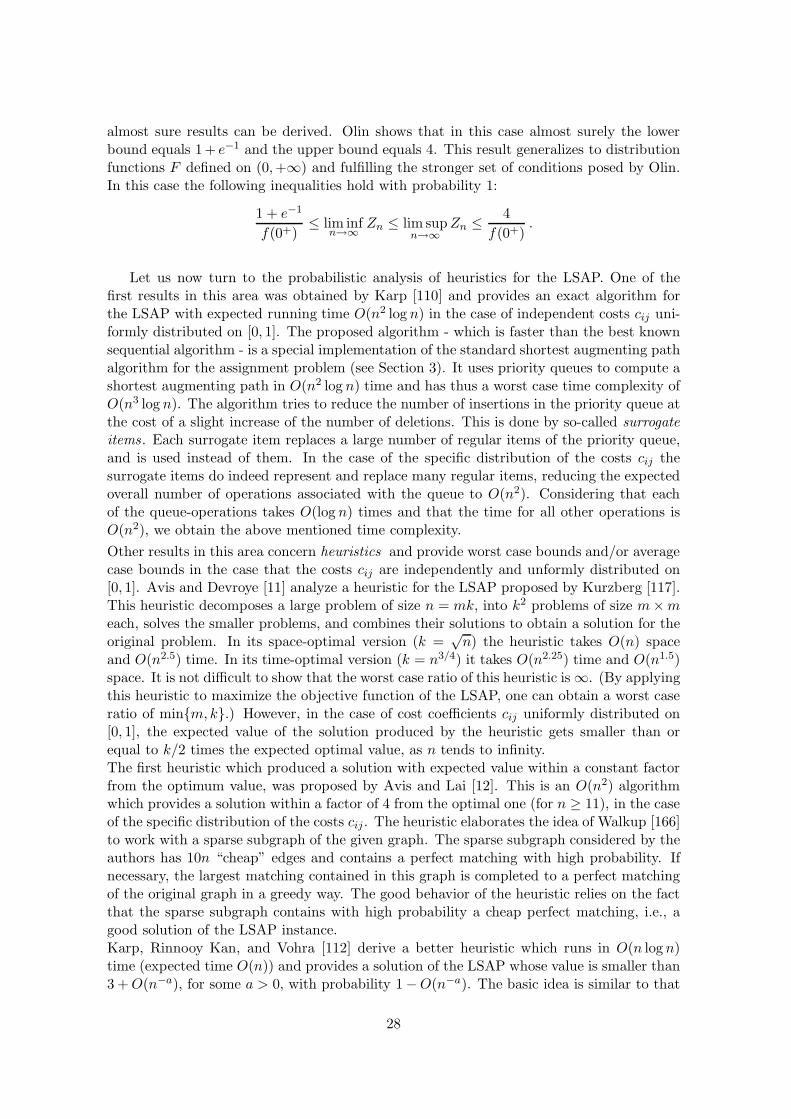
almost sure results can be derived. Olin shows that in this case almost surely the lowerbound equals 1+ e−1 and the upper bound equals 4. This result generalizes to distributionfunctions F defined on (0,+∞) and fulfilling the stronger set of conditions posed by Olin.In this case the following inequalities hold with probability 1:

1 + e−1

f(0+)≤ lim inf

n→∞Zn ≤ lim sup

n→∞Zn ≤ 4

f(0+).

Let us now turn to the probabilistic analysis of heuristics for the LSAP. One of thefirst results in this area was obtained by Karp [110] and provides an exact algorithm forthe LSAP with expected running time O(n2 log n) in the case of independent costs cij uni-formly distributed on [0, 1]. The proposed algorithm - which is faster than the best knownsequential algorithm - is a special implementation of the standard shortest augmenting pathalgorithm for the assignment problem (see Section 3). It uses priority queues to compute ashortest augmenting path in O(n2 log n) time and has thus a worst case time complexity ofO(n3 log n). The algorithm tries to reduce the number of insertions in the priority queue atthe cost of a slight increase of the number of deletions. This is done by so-called surrogateitems. Each surrogate item replaces a large number of regular items of the priority queue,and is used instead of them. In the case of the specific distribution of the costs cij thesurrogate items do indeed represent and replace many regular items, reducing the expectedoverall number of operations associated with the queue to O(n2). Considering that eachof the queue-operations takes O(log n) times and that the time for all other operations isO(n2), we obtain the above mentioned time complexity.

Other results in this area concern heuristics and provide worst case bounds and/or averagecase bounds in the case that the costs cij are independently and unformly distributed on[0, 1]. Avis and Devroye [11] analyze a heuristic for the LSAP proposed by Kurzberg [117].This heuristic decomposes a large problem of size n = mk, into k2 problems of size m×meach, solves the smaller problems, and combines their solutions to obtain a solution for theoriginal problem. In its space-optimal version (k =

√n) the heuristic takes O(n) space

and O(n2.5) time. In its time-optimal version (k = n3/4) it takes O(n2.25) time and O(n1.5)space. It is not difficult to show that the worst case ratio of this heuristic is ∞. (By applyingthis heuristic to maximize the objective function of the LSAP, one can obtain a worst caseratio of min{m,k}.) However, in the case of cost coefficients cij uniformly distributed on[0, 1], the expected value of the solution produced by the heuristic gets smaller than orequal to k/2 times the expected optimal value, as n tends to infinity.The first heuristic which produced a solution with expected value within a constant factorfrom the optimum value, was proposed by Avis and Lai [12]. This is an O(n2) algorithmwhich provides a solution within a factor of 4 from the optimal one (for n ≥ 11), in the caseof the specific distribution of the costs cij . The heuristic elaborates the idea of Walkup [166]to work with a sparse subgraph of the given graph. The sparse subgraph considered by theauthors has 10n “cheap” edges and contains a perfect matching with high probability. Ifnecessary, the largest matching contained in this graph is completed to a perfect matchingof the original graph in a greedy way. The good behavior of the heuristic relies on the factthat the sparse subgraph contains with high probability a cheap perfect matching, i.e., agood solution of the LSAP instance.Karp, Rinnooy Kan, and Vohra [112] derive a better heuristic which runs in O(n log n)time (expected time O(n)) and provides a solution of the LSAP whose value is smaller than3 +O(n−a), for some a > 0, with probability 1−O(n−a). The basic idea is similar to that

28

of Avis and Lai: Construct a “cheap” sparse subgraph of the given graph and show that itcontains a perfect matching with high probability. Again, if the subgraph does not containa perfect matching a solution for the original LSAP instance is determined in a greedy way.The subgraph is introduced in terms of so-called random 2-out bipartite graphs. Such agraph contains a perfect matching with probability 1 − O(n−a) and the matching can befound in O(n log n) time. Further, it is shown how to construct a random 2-out bipartitesubgraph with cheap edges for the given LSAP instance. The expected value of a solutionobtained either as a perfect matching in this subgraph, or by applying a greedy approach,if the former does not exist, equals 3 +O(n−a).

5 Bottleneck Assignment Problems

As mentioned in Section 2 linear bottleneck assignment problems (LBAP)

minφ

max1≤i≤n

ciφ(i) (15)

occur in connection with assigning jobs to parallel machines so as to minimize the latestcompletion time. The first authors who considered bottleneck assignment problems wereFulkerson, Glicksberg and Gross [84]. Gross [98] proved the following duality result forLBAPs which gave rise to the theory of blocking systems, see Edmonds and Fulkerson [73].

Theorem 5.1 (Gross [98], 1959)Let N = {1, 2, . . . , n} and let Sn be the set of all permutations φ of N . Then, for anarbitrary n× n matrix C = (cij) of real numbers

minφ∈Sn

maxi∈N

ciφ(i) = maxA,B⊆N

|A|+|B|=n+1

mini∈A,j∈B

cij . (16)

So-called threshold algorithms play an important role to solve LBAPs. A thresholdalgorithm alternates between two phases. In the first phase a cost element c∗ij - the thresholdvalue - is chosen and a matrix C is defined by

cij :=

{

1 if cij > c∗ij

0 if cij ≤ c∗ij

In the second phase it is checked, whether the bipartite graph with adjacency matrix Ccontains a perfect matching or not. The smallest value c∗ij for which the correspondingbipartite graph contains a perfect matching, is the optimum value of the LBAP (15).There are several ways to implement such a threshold algorithm. One possibility is to orderthe cost elements increasingly and to apply a binary search, in the first phase. This leads toan O(T (n) log n) algorithm, where T (n) is the time complexity for checking the existenceof a perfect matching. Concerning T (n) see the remarks after Theorem 1.3 in Section 1.Another possibility is to mimic the Hungarian method. We start with

c∗ := maxi,j

(mini

cij , minj

cij) (17)

and grow bottleneck augmenting paths as long as the matrix C does not contain an as-signment with objective function value equal to 0, see Page [134], Garfinkel [88], Derigsand Zimmermann [70], Carpaneto and Toth [55] and Derigs [67]. FORTRAN codes for

29

this method can be found in the book by Burkard and Derigs [39] and in Carpaneto andToth [55]. The implementations differ in the determination of a starting solution and inthe applied data structures. One of the most efficient implementations is described inDerigs [67]. A similar approach using the framework of strong spanning trees (see also Sec-tion 3 and Balinski and Gonzalez [21]) is given by Armstrong and Jin [10]. Their algorithmcan be implemented within a running time of O(mn + n2 log n) , where m is the numberof finite entries in matrix C, i.e., the number of edges of the bipartite graph G associatedwith the assignment problem.

An algorithm with the currently best time complexity is obtained by combining thethreshold approach with augmenting paths. This idea goes back to Gabow and Tarjan [87],who gave an algorithm for LBAP with worst case complexity O(m

√n log n). For dense

graphs this bound has been further improved by Punnen and Nair [150]. According tothese authors we first solve

minM∈F ∗

max(i,j)∈M

cij , (18)

where F ∗ is the set of all matchings in G which differ from a maximum matching by at mostn√

n/m edges. Combining the maximum matching algorithm of Alt et al. [9] (see Section1) with binary search, this problem can be solved in O(n1.5√m) time. Then this solutionis extended to a optimal solution of the bottleneck assignment problem by growing at mostn√

n/m augmenting paths. Every augmenting path can be completed in O(m) time, seee.g. Tarjan [159]. Thus the overall complexity of the algorithm becomes O(n

√nm).

Pferschy [139] describes an algorithm with expected running time O(n2), i.e., linear onm in the case that the graph G is dense. In a first step the given graph is thinned outby considering only the 2n log n cheapest edges. This can be done in O(n2) time by usinga linear selection algorithm for finding the 2n log n-smallest edge. In the second step theLBAP on the sparse subgraph is solved by using the method of Gabow and Tarjan. Thisyields O((n log n)3/2) additional elementary operations. Finally the solution is completedto a perfect matching of the full graph by applying again the algorithm of Gabow andTarjan. But this completion step is only necessary with a low probability, namely with aprobability less than O(1/

√n log n). Thus, the expected time needed by the completion is

O(n2), and we get an overall expected running time of O(n2). This algorithm provides notonly a good bound in terms of complexity, but is also very efficient and simple to use.

In a detailed study Pferschy [140] compared different (deterministic) solution proceduresfor LBAPs up to n = 2000. He observed that the fastest algorithm with respect to theoverall running time consists of computing a lower bound for the optimal solution value,e.g. by (17), then finding a maximum matching (using the Hopcroft-Karp procedure) in thesubgraph consisting of the edges with weight less or equal to this bound, and finally aug-menting this matching. Moreover, Pferschy noticed that the selection of a sparse subgraphtakes a considerable amount of time, whereas not much computational efforts are neededto solve the LBAP in sparse subgraphs.

There are again some simple cases when an optimal solution of the LBAP can be givenbefore hand. As in Section 2 these cases are related to Monge properties of the cost matrixC.

Matrix C = (cij) is said to be a bottleneck Monge matrix (cf. Burkard et al. [42]), if itfulfills the following conditions:

max{cij , ckl} ≤ max{cil, ckj} , for 1 ≤ i < k ≤ n, 1 ≤ j < l ≤ n. (19)

30

It is easy to show that the identical permutation is an optimal solution of an LBAP witha bottleneck Monge cost matrix. An analogous result holds for inverse bottleneck Mongematrices defined by

max{cij , ckl} ≥ max{cil, ckj} , for 1 ≤ i < k ≤ n, 1 ≤ j < l ≤ n. (20)

LBAPs with an inverse bottleneck Monge cost matrix are solved by the permutation φ(i) =n − i + 1, for all i. The recognition of permuted bottleneck Monge matrices, however, ismore difficult than solving the bottleneck assignment problem directly, see Klinz, Rudolf,and Woeginger [115], and Burkard et al. [42].

In Pferschy [139] the asymptotic behavior of the LBAP is studied. Pferschy shows thatthe expected value of the optimal solution of an LBAP with independently and identicallydistributed costs tends towards the infimum of the cost range as the size of the problemtends to infinity. He derives explicit lower and upper bounds for the optimum value of anLBAP of size n.

Besides the classical application in scheduling theory bottleneck assignment problemshave also been used in connection with time slot assignment problems (see the descriptionof the telecommunication problem in the earth-satellite systems, Section 2). One variant ofthe time slot assignment problem is to decompose the given traffic matrix in a weighted sumof at most n permutation matrices such that T ≤ ∑n

k=1 λkPk, λk ≥ 0 holds and∑nk=1 λk

is minimum. Balas and Landweer [13] propose a heuristic for this NP-hard problem: solvea series of bottleneck assignment problems in order to determine the weights λk.

A multi-level bottleneck assignment problem has been considered by Carraresi andGallo [50] in connection with the bus drivers’ rostering problem: Daily shifts are to beassigned to bus drivers. To each shift a weight is assigned. This weight represents the costof the shift for the drivers, e.g., length of the shift, lateness, time to reach the startingpoint etc. The problem of finding an equal balance of the shifts leads to minimizing thetotal weight of the shifts assigned to a single driver. For solving this NP-hard optimizationproblem the authors propose to solve a sequence of bottleneck assignment problems.

Lexicographic bottleneck assignment problems (LexBAP) have been considered byBurkard and Rendl [43]. Let C = (cij) be a real n × n matrix and let φ be a permutationof the set {1, 2, . . . , n}. Now let cφ be the vector where the n cost coefficients ci,φ(i),1 ≤ i ≤ n, are ordered decreasingly. The lexicographic bottleneck assignment problem asksfor a solution φ∗ with

cφ∗ = lexminφ∈Sncφ.

The authors propose two solution approaches. The first one scales the cost coefficientsand transforms the LexBAP in a sum assignment problem. (A similar transformation ofbottleneck assignment problems in sum assignment problems had already been proposed byPage [134]). In a second approach the LexBAP is iteratively solved by a series of bottleneckand sum assignment problems. If the LexBAP has k distinct cost coefficients and we denotethe computational complexity of the sum assignment problem by T (n), then LexBAP can besolved in O(T (n)n2 log k) time. Bardadym [25] suggested the following improved algorithm.Order the k distinct cost elements decreasingly and represent any cost coefficient cij by avector dij = (d1

ij , d2ij , . . . , d

kij) with k elements, where drij = 1, if cij is the r−largest cost

coefficient, and drij = 0, otherwise. In this model the lexicographic bottleneck assignmentproblem becomes a lexicographic vector assignment problem which fits in the frameworkof algebraic assignment problems (see Section 6). The solution of this problem involvesO(kT (n)) elementary operations.

31

Balanced assignment problems have been considered by Martello, Pulleyblank, Toth,and de Werra [125]. Given a real n×n matrix C = (cij), the balanced assignment problemcan be formulated as

minφ

[

maxiciφi − min

iciφi

]

.

For solving this problem the authors sort the entries cij non-decreasingly and propose thefollowing O(n4) procedure:

1. Solve the corresponding bottleneck assignment problem. Let φ∗ be its optimal solu-tion.

2. Definel := min

iciφ∗(i), u := max

iciφ∗(i).

If l = u, stop. A balanced solution has been found. Otherwise go to Step 3.

3. Delete in C all elements ≤ l and > u and grow augmenting paths.If there exists a perfect matching, set φ∗ equal to that solution and go to Step 2. Ifno solution exists, then go to Step 4.

4. If u is already the maximum element of matrix C, stop. The present solution isoptimal. Otherwise increase u to the next larger element and return to Step 3.

6 Assignment Problems with Other ObjectiveFunctions

As pointed out by Burkard, Hahn, and Zimmermann [41], sum and bottleneck assignmentproblems are just special cases of a more general problem, the so-called algebraic assignmentproblem which can also be solved efficiently.

Let (H, ∗,≺) be a totally ordered commutative semigroup with composition ∗ and orderrelation ≺. The algebraic assignment problem (AAP) with cost coefficients cij ∈ H can beformulated as

minφ∈Sn

c1φ(1) ∗ c2φ(2) ∗ · · · ∗ cnφ(n) . (21)

For deriving efficient solution procedures we require some additional properties for (H, ∗,≺).We assume that the order relation is compatible with the composition, i.e.,

a ≺ b⇒ a ∗ c ≺ b ∗ c for a, b, c ∈ H ,

and that H is a so-called d-monoid , i.e.,

a ≺ b ⇒ there exists c ∈ H such that a ∗ c = b.

As we will see below, under these conditions the AAP can be solved in O(n4) time. Ifwe additionally require that the weak cancellation rule

if a ∗ c = b ∗ c, then either a = b or a ∗ c = b

applies, the complexity can be improved to O(n3), see Burkard and Zimmermann [46]. Forfurther results in this direction, consult the survey on algebraic optimization by Burkardand Zimmermann [47].

Special models for d-monoids are:

32

• H = IR with addition as composition and the usual (or inverse) order relation. Thismodel leads to sum assignment problems (with a minimization or a maximizationobjective function).

• H is the set of extended real numbers IR (including −∞) with the usual order relation.The composition is defined by a ∗ b := max (a, b). This model leads to bottleneckassignment problems.

• H = IRn, the composition is the vector addition and the order relation is the lexico-graphical order. This leads to lexicographical sum assignment problems.

• H = IR × IR, ≺ is the lexicographical order and the composition is defined by

(a, b) ∗ (c, d) :=

{

(a, b) if a ≥ c

(a, b+ d) if a = c

This leads to the so-called time-cost assignment problem, where a duration measuretij and a cost cij are assigned under these conditions to each pair (i, j). Among allassignments which minimize the overall duration we seek for one which minimizes theoverall cost.

• H = [0, 1], the order relation is the usual “greater than or equal to” order ≥, andthe composition is the multiplication of real numbers. This model leads to reliabilityassignment problems: max Πn

i=1aiφ(i) over all permutations φ of 1, 2, . . . , n.

Algebraic assignment problems can be solved by performing admissible transformations.Let us denote

z[C,φ] := c1,φ(1) ∗ c2,φ(2) ∗ · · · ∗ cn,φ(n) .

Definition 6.1 (Admissible transformations)A transformation T of the n×n matrix C = (cij) to the matrix C = (cij) is called admissiblewith index z(T ), if

z[C,φ] = z(T ) ∗ z[C, φ]

for all φ ∈ Sn.A composition of admissible transformations S and T with indices z(S) and z(T ), re-spectively, is again an admissible transformation with index z(S) ∗ z(T ). Now we get thefollowing optimality criterion:

Theorem 6.2 Let T : C 7→ C be an admissible transformation such that there exists apermutation φ with the following properties:

1. z(T ) ∗ cij ≥ z(T )

2. z[C, φ] ∗ z(T ) = z(T ).

Then φ is an optimal assignment with value z(T ).

Proof. Let φ be an arbitrary permutation. According to Definition 6.1 and properties (1)and (2) of the proposition above we get:

z[C,φ] = z(T ) ∗ z[C, φ] ≥ z(T ) = z(T ) ∗ z[C, φ] = z[C, φ]

Therefore φ is optimal.

Admissible transformations for assignment problems are described by the following theorem:

33

Theorem 6.3 (Admissible transformations for assignment problems [41], 1977)Let I, J ⊆ {1, 2, . . . , n}, m := |I| + |J | − n ≥ 1, and c := min{cij : i ∈ I, j ∈ J}. Then the

transformation C 7→ C defined by

cij ∗ c = cij , for i ∈ I, j ∈ J

cij = cij ∗ c , for i 6∈ I, j 6∈ J

cij = cij , otherwise

is admissible with z(T ) = c∗ c∗ · · · ∗ c, where the expression on the right hand-side containsm factors.

For solving an algebraic assignment problem we can use now the following procedure:

1. Perform row reductions, i.e., perform admissible transformations with I = {i}, J ={1, 2, . . . , n}. Start with i = 1 and let z := z(T ) be the corresponding index. Continuewith i = 2, . . . , n and update z := z∗z(T ). Afterwards all elements are “nonnegative”,namely cij ∗ z ≥ z.

2. Perform column reductions, i.e., perform admissible transformations with J = {j}, I ={1, 2, . . . , n},, for j = 1, 2, . . . , n. Afterwards every row and column contains at leastone generalized 0-element , i.e., an element which fulfills

z ∗ cij = z .

3. Determine a maximum matching in subgraph of the bipartite graph associated withthe assignment problem, which contains only the edges corresponding to the general-ized 0-elements, (cf. Theorem 1.6).

4. If the maximum matching is perfect, then stop: the optimal solution is given by thismatching and z is the optimal value of the objective function.Otherwise, go to Step 5.

5. Determine a minimum cover of the “0-elements”. This cover yields the new indexsets I and J . I contains the indices of the uncovered rows, J contains the indices ofuncovered columns.

6. Perform an admissible transformation determined by the new index sets I and J asin Theorem 6.3, update z := z ∗ z(T ), and go to Step 3.

It is rather straightforward to show that this algorithm yields after at most n2 − 2n + 3admissible transformations an optimal solution of the algebraic assignment problem. If thecomposition ∗ is specialized to “+”, it becomes a variant of the Hungarian method. If thecomposition is specialized to the max operation, then we obtain the bottleneck assignmentproblem and the above algorithm is a variant of the threshold method.

Analogously to (sum) Monge and bottleneck Monge matrices, we can also define Mongematrices in the case that cij are taken from the ordered semigroup H, cf. Burkard et al. [42].The AAP with an algebraic Monge cost matrix is again solved to optimality by the identitypermutation. The problem of recognizing permuted algebraic Monge matrices is rathersubtle. Woeginger [169] has shown that this problem is NP-hard, if n ≥ 3 and the ordered

34

semigroup fulfills no additional property. It becomes polynomially solvable, if e.g. a weakcancellation rule of the form

a ∗ c = b ∗ c⇒ a = b or a ∗ c = c , for a, b, c ∈ H

is fulfilled. For details see Burkard et al. [42].

7 Available computer codes and test instances

FORTRAN listings of a primal-dual algorithm for the LSAP, based on shortest path com-putations done by a version of Dijkstra’s algorithm, can be found in the book by Burkardand Derigs [39]. In that book there is also a code of an algorithm for the linear bottleneckassignment problem (LBAP). This algorithm is obtained as an adaptation of the abovementioned LSAP algorithm to the LBAP, and is described in detail by Derigs and Zim-merman [70]. The differences between the two algorithms are discussed by Burkard andZimmermann [46].

Source codes of another primal-dual algorithm for the LSAP can be downloaded fromhttp://207.158.230.188/assignment.html. One can choose among a C++, a PASCAL,and a FORTRAN implementation of the algorithm of Jonker and Volgenant [108] for denseLSAPs, and among a FORTRAN and a PASCAL implementation for sparse LSAPs. Thereare also PASCAL and FORTRAN codes of an adaptation of the above mentioned algorithmto the LBAP. All codes are available as zip files.

A (compressed) FORTRAN source file - called 548.Z - of an implementation of the Hun-garian algorithm, due to Carpaneto and Toth [54], can be downloaded fromftp://netlib.att.com in /netlib/toms. Other listings of FORTRAN codes for the LSAPcan be found in Carpaneto, Martello, and Toth [51]. These codes are also available fromthe floppy disc included in the book [51].

The C code (compressed tar) of an efficient implementation of the scaling push-relabel algo-rithm of Goldberg and Kennedy [94] for the LSAP can be downloaded from Goldberg’s net-work optimization library at http://www.neci.nj.nec.com/homepages/avg/soft.html.

Finally, listings of 5 FORTRAN codes of auction algorithms for the LSAP can be found inBertsekas’ homepage at http://web.mit.edu/dimitrib/www/auction.txt.The codes are: AUCTION - a forward auction algorithm for symmetric assignment problems,i.e., problems where the cost matrix is symmetric,AUCTION FLP - a version of AUCTION which emploies floating point arithmetic, AUCTION AS

- an auction algorithm for the asymmetric LSAP, AUCTION FR - a forward-reverse auctionalgorithm for symmetric LSAPs, and NAUCTION SP - a combination of the naive auctionalgorithm with sequential shortest paths methods.

Test instances of the LSAP can be downloaded as ascii files from the homepage of theOR-Library maintained by J. Beasley at http://mscmga.ms.ic.ac.uk/pub.Other test instances can be obtained as ascii or uuencoded files from the ELIB library at

ftp://ftp.zib.de/pub/Packages/mp-testdata/assign/index.html.

Let us notice that due to the equivalent formulation of the LSAP as a minimum costflow problem, algorithms developed for the later can also be applied to the LSAP. How-ever, such algorithms are not supposed to exploit the specific features of the LSAP, and

35

hence may not be competitive with algorithms developed especially for the LSAP. BesidesGoldberg’s network optimization library and Bertsekas’ homepage, other codes for networkoptimization can be found in Netlib at

http://www.OpsResearch.com/OR-Links/index.html.Furthermore, C codes (compressed tar files) of implementations of the primal and the dualnetwork simplex algorithm, due to Lobel, can be obtained through

http://www.zib.de/Optimization/index.de.html.

8 Multidimensional Assignment Problems

8.1 General Remarks and Applications

Multi-dimensional (sometimes referred as multi-index ) assignment problems (MAP) arenatural extensions of the linear assignment problem. They have been considered for thefirst time by Pierskalla [143]. The most prominent representatives of this class are axialand planar 3-dimensional assignment problems, which are treated in the subsections below.The general formulation of the MAP is

minn∑

i1=1

· · ·n∑

iN=1

ci1···idxi1···id

s.t.n∑

i2=1

· · ·n∑

id=1

xi1···id = 1, i1 = 1, . . . , n, (22)

n∑

i1=1

· · ·n∑

ik−1=1

n∑

ik+1=1

· · ·n∑

id=1

xi1···id = 1,

for k = 2, . . . , d− 1, and ik = 1, 2, . . . , n,n∑

i1=1

· · ·n∑

id−1=1

xi1···id = 1, id = 1, . . . , n,

xi1···id ∈ {0, 1} for 1 ≤ i1, i2, . . . id ≤ n,

with nd cost coefficients ci1···id .Differently stated the MAP asks for d − 1 permutations φ1, φ2, . . . , φd−1 such that theobjective function becomes minimum:

minφ1,φ2,...,φd−1

n∑

i=1

ciφ1(i)φ2(i)...φd−1(i) .

The multidimensional assignment problem is NP-hard in general, but in the case thatthe array of the cost coefficients is a Monge array (see [42]), it is solved by the identicalpermutations φi = id, for i = 1, 2, . . . , d − 1. A slightly weaker condition is considered inFortin and Rudolf [79]. Burkard, Rudolf and Woeginger [45] have shown, however, thatthe MAP remains NP-hard for d ≥ 3 , if the cost array is inverse Monge. This impliesthat maximizing the objective function with cost elements drawn from a Monge array isNP-hard.In terms of graphs a multidimensional assignment problem can be described as follows:Let a complete d-partite graph G = (V1, V2, . . . , Vd;E) with vertex sets Vi, |Vi| = n, i =1, 2, . . . , d, and edge set E be given. A subset X of V =

⋃di=1 Vi is a clique, if it meets

every set Vi in exactly one vertex. A d-dimensional assignment is a partition of V into n

36

pairwise disjoint cliques. If c is a real valued cost function defined on the set of cliquesof G = (V1, V2, . . . , Vd;E), the d-dimensional assignment problem asks for a d-dimensionalassignment of minimum cost.

Bandelt, Crama, and Spieksma [24] consider cases where the costs c of a clique are notarbitrary, but given as a function of elementary costs attached to the edges of the completed-partite graph. The costs of a clique considered in [24] are sum costs (sum of the lengthsof edges induced by the clique), star costs (minimum length of a spanning star), tour costs(minimum cost of a traveling salesman tour in the clique), and tree costs (minimum cost of aspanning tree in the clique). The authors derive worst case bounds on the ratio between thecosts of solutions obtained by applying simple heuristics and the costs of optimal solutionsfor these special MAPs.

Multidimensional assignment problems in their general form have recently found someapplications as a means to solve data association problems. More specifically, the centralproblem in any multi-target tracking and multi-sensor surveillance is the data associationproblem of partitioning the observations into tracks and false alarms in real time. Generalclasses of these problems can be formulated as multidimensional assignment problems. Inthe following we briefly describe such a formulation for a multi-target tracking problem.The reader is referred to Poore, Rijavec, Liggins, and Vannicola [147] for more details and analternative derivation of the multidimensional assignment formulation. In a target trackingprocess we collect reports from different measurements performed at discrete moments intime denoted by 1, 2, . . . , n. Let us denote by Z(k) a data set of Mk reports (dummy ormissing reports are included) obtained by measurements at time k, and let Zn denote thecumulative set of Z(k), k = 1, 2, . . . , n,

Z(k) = {zkik}Mkik=0 , Zn = {Z(1), Z(2), . . . , Z(n)} .

The index ik = 0 is reserved for missing reports. We are looking for a feasible partitionγ of the data set Zn into data tracks corresponding to different objects and false alarms,which leads to a best possible reproduction of the real life situation. A feasible partitionγ = {γ1, γ2, . . . , γn(γ)} consists of n(γ) tracks γj, 1 ≤ j ≤ n(γ) of reports. Each track γjof a partition γ is given as γj = {z1

i1, z2i2, . . . , znin} and is defined in terms of the properties

it fulfills. First the different tracks may have only missing or dummy reports in common,and no track consists of only dummy reports:

γi ∩ γj ⊂ {z10 , z

20 , . . . , z

n0 } , for i 6= j , and γj 6= {z1

0 , z20 , . . . , z

n0 } , for all j

Further, the union of all tracks together with the track consisting of only dummy reportscovers the cumulative set of data Zn, and each track contains at least one report from theset Z(k), 1 ≤ k ≤ n:

Zn =[

∪n(γ)j=1 γj

]

∪ {z10 , z

20 , . . . , z

n0 } , γj ∩ Z(k) 6= ∅ , for all j, k.

Now we can use 0-1 variables xi1i2...in to characterize a feasible partition γ, where

xi1i2...in =

{

1 if {z1i1 , z

2i2 , . . . , z

nin} ∈ γ

0 otherwise

and the following equalities are fulfilled

M1,M2,...,Mk−1,Mk+1,...,Mn∑

i1,i2,...,ik−1,ik+1,...,in

xi1i2...in = 1 , for k = 1, 2, . . . , n .

37

It is clear that these equalities are similar to those in the formulation (22) of the MAP givenearlier in this section. In the special case where all Mi have a common value we obtain theconstraints of (22).

Let us turn now to the modeling of the objective function. Let γ0 be a reference partition,e.g. the partition consisting of all false reports, and let P (γ|Zn) be the probability of apartition γ given the data set Zn. Without going into details - for which the user is referredto [147] - notice that the maximization of P (γ|Zn)/P (γ0|Zn) over all feasible partitions γwould be a reasonable objective function from the physical point of view. Under naturalprobabilistic assumptions on the space of feasible partitions it can be assumed that

P (γ|Zn)P (γo|Zn)

= Lγ =∏

{z1i1,z2

i2,...,zn

in}∈γ

Li1i2...in ,

where each likelihood ratio Li1i2...in ≡ L(z1i1 , z

2i2 , . . . , z

nin) depends only on the sequence of

reports {z1i1 , z

2i2 , . . . , z

nin} and not on the partition in which this sequence occurs. (The

reader is referred to Poore and Rijavec [146] for a complete list of assumptions under whichthis decomposition is allowed.) By introducing ci1i2...in := − lnLi1i2...in for all i1, i2, . . . , inwe get

−ln[

P (γ|Zn)P (γ0|Zn)

]

=∑

{z1i1,z2

i2,...,zn

in}∈γ

ci1i2...in . (23)

Then the maximization of P (γ|Zn)/P (γ0|Zn) is equivalent to the minimization of the sumin the right hand-side of (23).

For other applications of MAPs in target tracking problems, like track initiation andtrack maintenance, or multi-sensor tracking, the reader is referred to Poore [144] and thereferences therein. Some Lagrangian relaxation algorithms for the MAP have been devel-oped by Poore and Rijavec [146] and Poore and Robertson [148]. These algorithms relax oneor more constraints and derive a set of good Lagrangean multipliers, e.g. by standard non-smooth optimization techniques, in a first phase. In a second phase they involve a so-calledrecovery procedure to construct a good feasible solution of the original problem startingfrom an optimal (or good) solution of the relaxed problem with values of Lagrangean multi-pliers determined in the first phase. A numerical study of data association problems arisingin multi-target and multi-sensor tracking is given in Poore [145].

Pusztaszeri, Rensing, and Liebling [149] describe another interesting MAP which arisesin the context of tracking elementary particles. By solving a five-dimensional assignmentproblem, they reconstruct tracks generated by charged elementary particles produced bythe Large Electron-Positron Collider (LEP) at CERN institute.

8.2 Axial 3-Dimensional Assignment Problems

Consider n3 cost coefficients cijk. The axial 3-dimensional assignment problem (3-DAP)can then be stated as

minn∑

i=1

n∑

j=1

n∑

k=1

cijkxijk

s.t.n∑

j=1

n∑

k=1

xijk = 1 , i = 1, 2, . . . , n ,

38

n∑

i=1

n∑

k=1

xijk = 1, i = 1, 2, . . . , n , (24)

n∑

i=1

n∑

j=1

xijk = 1, i = 1, 2, . . . , n ,

xijk ∈ {0, 1} ∀ 1 ≤ i, j, k ≤ n .

The name stems from the model which assigns the 1-s on the right hand-side to distinctpositions at the axes of a 3-dimensional array. The sum over the corresponding “flat” inthe array must equal the amount assigned to the position on the axis, see Fig. 5. We can

b)

1 1 11

1

1

1

1

1

i

j

k

1 1 1

1 1 1

1 1 1

1

11 1

11

1

11

11

1

1

11

11

1

i

k

j

a)

Figure 5: a) A geometric representation of the axial 3-dimensionalassignment problem for n = 3. b) A geometric representation ofthe planar 3-dimensional assignment problem for n = 3.

think of cijk as the cost of assigning job j to be performed by worker i in machine k. Itfollows that xijk = 1, if job j is assigned to worker i in machine k, and xijk = 0, otherwise.A feasible solution of the above problem will be a three dimensional permutation array ,i.e., a 0-1 array that satisfies the above assignment constraints.Equivalently, a 3-DAP can be described with the help of two permutations φ and ψ

minφ,ψ∈Sn

n∑

i=1

ciφ(i)ψ(i). (25)

Thus this problem has (n!)2 feasible solutions. Karp [109] showed that the 3-DAP is NP-hard in contrast to the sum linear assignment problem (LSAP).

In terms of graph theory, the 3-DAP can be stated as follows: Given a complete 3-partitegraph Kn,n,n with disjoint vertex sets U ,V , and W , find a subset A of n triangles, A ⊆U × V ×W , such that every element of U ∪ V ∪W occurs in exactly one triangle of A andthe total cost

∑

(i,j,k)∈A cijk is minimized.

Euler [75] started the investigation of the axial 3-index assignment polytope (i.e., theconvex hull of feasible solutions to problem (24)) by considering the role of odd cycles fora class of facets of this polytope. Independently Balas and Saltzman [16] investigate indetail the polyhedral structure of the three-index assignment polytope, and show that thispolytope has dimension n3−3n+2. They describe an O(n4) separation algorithm for facetsinduced by certain cliques. Balas and Qi [15] continue the above work and present O(n3)separation algorithms for earlier identified classes of facets as well as for a new class offacets. (Note that since there are n3 variables these are linear-time algorithms). Qi, Balas,

39

and Gwan [151] base their work on linear-time separation algorithms for different facetsand construct a polyhedral procedure for solving the 3-DAP.

Pierskalla [142] was the first, who proposed a heuristic for solving 3-DAP. As for algorithmsto solve the 3-DAP to optimality, branch and bound is a classical one. Most of the al-gorithms split the current problem into two subproblems by fixing one variable xijk to 1and to 0, respectively. In this way the size of the first subproblem decreases. Balas andSaltzman [17] have introduced a branching strategy that exploits the structure of the prob-lem and allows to fix several variables at each branching node. Burkard and Rudolf [44]experiment with different branch and bound schemes for the 3-DAP. In particular, theyinvestigate branching rules stemming from the polyhedral description of the underlyingpolytope, see Balas and Saltzman [16].

Hansen and Kaufman [100] describe a primal-dual method similar to the Hungarian methodfor linear assignment problems. In the case of 3-DAPs, hypergraphs have to be consideredinstead of bipartite graphs. First as many 0-elements as possible are generated among thecost coefficients by generalized row- and column reductions. Then a covering problem issolved for these 0-elements. If the covering number is smaller than n, further 0-elementsare generated by means of an admissible transformation similar to those in Section 6. Ifthe covering number equals n, the corresponding stability problem is solved. Notice thatfor hypergraphs the minimum number of (hyper-)edges in a cover is in general strictlylarger than the cardinality of a stable set, and this is an inherent difficulty for this problemclass. If the stability number equals n, an optimal solution has been found, otherwise abranching is performed. Note the similarity of this method with the approach in Section 6for solving algebraic assignment problems. Due to this similarity the same algorithm solvesthe “algebraic” version of the 3-DAP with cost coefficients drawn from a d-monoid. Thesubproblems of finding a minimum cover and a maximum stable set are in this case, however,NP-hard.

Admissible transformations for 3-DAP are described by the following theorem due toBurkard and Frohlich [40]. Let us first introduce some notation. Let N := {1, 2, . . . , n},I,J ,K ⊆ N and denote I := N \ I J = N \ J , K = N \K. With these definitions we get

Theorem 8.1 (Admissible transformations for the 3-DAP [40], 1980Let a 3-DAP with cost coefficients cijk, i, j, k = 1, 2. . . . , n, be given. For I, J,K ⊆ N withm := n− (|I| + |J | + |K|) ≥ 1 and

c := min{cijk: (i, j, k) ∈ I × J × K}

we define

cijk := cijk − c , (i, j, k) ∈ I × J × K

cijk := cijk + c , (i, j, k) ∈ (I × J ×K) ∪ (I × J ×K) ∪ (I × J × K)

cijk := cijk + 2c , (i, j, k) ∈ I × J ×K

cijk := cijk , otherwise

Then, for any feasible solution φ,ψ of the 3-DAP we have

n∑

i=1

ciφ(i)ψ(i) =n∑

i=1

ciφ(i)ψ(i) +mc.

40

Clearly, row and column reductions are special cases of the admissible transformationsdescribed by the above theorem.

Strong lower bounds are essential for a branch and bound procedure. One of the ap-proaches used to compute lower bounds for the 3-DAP is Lagrangean relaxation. By takingtwo blocks of the constraints of a 3-DAP into the objective function via Lagrangean mul-tipliers, we get a Lagrangian relaxation of (24) (cf. [40]):

L(π, ǫ) := min

n∑

i=1

n∑

j=1

n∑

k=1

(cijk + πj + ǫi)xijk −n∑

j=1

πj −n∑

i=1

ǫi

such thatn∑

i=1

n∑

j=1xijk = 1 , k = 1, 2, . . . , n

xijk ∈ {0, 1} , 1 ≤ i, j, k ≤ n

π ∈ IRn, ǫ ∈ IRn .

L(π, ǫ) is a concave function, and a subgradient method can be used to find its maximum.Let r be a counter of iterations. Start with πr := ǫr := 0 for r = 0. In each iteration r usea greedy algorithm to minimize L(πr, ǫr). Let xrijk be the corresponding optimal solution.Define vri0 := |{xri0,j,k:xi0,j,k = 1}|−1 for i0 = 1, 2, . . . , n, and wrj0 := |{xri,j0,k:xi,j0,k = 1}|−1for j0 = 1, 2, . . . , n. If vr = wr = (0, 0, . . . , 0), then the maximum is reached. Otherwise πand ǫ are updated by setting

πr+1 := πr + λrwr, ǫr+1 := ǫr + λrv

r ,

where λ is a suitable step length λ. This procedure is repeated a prespecified number ofiterations.

Another subgradient procedure for solving a Lagrangean relaxation of the 3-DAP togetherwith computational considerations has been described by Frieze and Yadegar [83]. Burkardand Rudolf [44] report on satisfactory computational results obtained by an algorithm whichuses the classical branching rule combined with a reduction step in every node of the searchtree. The lower bound computation is done by applying the above described subgradientoptimization procedure. Another branch and bound algorithm proposed by Balas andSaltzman [17] solves another Lagrangean relaxation to compute the lower bounds. Thisrelaxation incorporates a class of facet inequalities and is solved by a modified subgradientprocedure. The upper bounds are computed by a primal heuristic based on the principle ofminimizing maximum regret, plus a variable depth interchange phase. A novel branchingstrategy fixes several variables at each node and reduces the size of the branching tree. Theauthors report on satisfactory numerical results.

There exists a number of polynomially solvable special cases of the 3-DAP. As mentionedin Section 8.1, the 3-DAP becomes polynomially solvable, if the cost coefficients are takenfrom a 3-dimensional Monge array (see [42]). Burkard, Rudolf, and Woeginger [45] inves-tigate 3-DAPs with decomposable cost coefficients, where cijk = uivjwk and ui, vj , and wkare nonnegative. It is shown that the maximization version of this problem is polynomiallysolvable, whereas the minimization is in general NP-hard. Moreover, several polynomiallysolvable special cases of the minimization problem are identified.

Crama and Spieksma [61] consider special cases of the graph theoretic formulation of the3-DAP. They assume that the lengths of the edges of the underlying 3-partite graph fulfill

41

the triangle inequality, and that the cost of a triangle is defined either as sum of the lengthsof its sides (problem T∆) or as sum of the lengths of the two shorter sides (problem S∆).The authors prove that the corresponding 3-DAPs are NP-hard. They design, however,heuristics which always deliver feasible solutions whose corresponding value of the objectivefunction is within 3/2 (4/3) from the optimal value, in the case of T∆ (S∆). of the optimalcost. Computational experiments show that the performance of these heuristics is verygood on randomly generated instances.

8.3 Planar 3-Dimensional Assignment Problems

Let n3 cost coefficients cijk be given. Planar 3-dimensional assignment problems (3-PAP)have the following form.

minn∑

i=1

n∑

j=1

n∑

k=1

cijkxijk

s.t.n∑

i=1

xijk = 1 , j, k = 1, 2, . . . , n , (26)

n∑

j=1

xijk = 1 , i, k = 1, 2, . . . , n ,

n∑

k=1

xijk = 1 , i, j = 1, 2, . . . , n ,

xijk ∈ {0, 1} i, j, k = 1, 2, . . . , n .

For a geometric interpretation of the 3-PAP see Fig. 5. Every “flat” in the three-dimensionalarray xijk must contain a (2-dimensional) assignment. Thus the feasible solutions of the3-PAP correspond to Latin squares. Fig. 6 shows a feasible solution for a 3-PAP withn = 3: number 1 represents the assignment in the lowest horizontal flat, number 2 showsthe assignment in the medium flat, and 3 represents the assignment in the upper flat. Dueto this interpretation, the number of feasible solutions of a 3-PAP of size n equals thenumber of Latin squares of order n, and hence increases very fast. The number of differentLatin squares of order d equals d!(d − 1)!T (d), where T (d) is the number of reduced Latinsquares. There is not much known about T (d), the largest value known so far seems to befor d = 9. T (9) =377,597,570,964,258,816 due to Bammel and Rothstein [23]. An explicitformula for the number of Latin squares of order d can be found in Shao and Wei [156],but this formula is difficult to evaluate.

Frieze [82] has shown that the 3-PAP is NP-hard. A description of the polyhedralstructure of the 3-PAP polytope has been given by Euler, Burkard, and Grommes [76].

3-PAPs have interesting applications in time tabling problems. A recent study on timetables and related polyhedra can be found in Euler and Verge [77].

There are not many algorithms known for the 3-PAP. The first branch and bound algo-rithm goes back to Vlach [163]. Vlach computes the lower bounds by applying (generalized)row and column reductions similar to those used in the case of 3-DAPs. Another branchand bound procedure for the planar 3-index assignment problem has been described byMagos and Miliotis [124]. To our knowledge this is the only paper reporting on compu-tational experience with an algorithm which solves the 3-PAP to optimality. The authorsuse a so-called relaxation heuristic to compute upper bounds by relaxing the third group of

42

2

ij

k1 2 3

132

3 1

Figure 6: A latin square representing a feasible solution ofthe planar 3-dimensional assignment problem of size n = 3.

constraints in (26). The remaining problem can be decomposed into n LSAPs, one for eachfixed value of the index k. These LSAPs are solved consecutively, and after solving each ofthem a number of variables are fixed so as to guarantee feasibility for the original problem.The so-found solutions are further improved by a local improvement procedure based onthe relationship between 3-PAPs and Latin squares. More precisely, the current solutionis presented as a Latin square and a cell of the Latin square is selected. The contents ofthis cell is changed according to some prespecified rule. Then, the contents of other cells ofthe Latin square is changed so as to obtain a new Latin square corresponding to a betterfeasible solution of the 3-PAP.The lower bounds are computed by a heuristic to solve the dual and - in a small numberof branch and bound nodes - also by solving a Lagrangean relaxation of the 3-PAP. Theheuristic for the dual is based on row and column reductions in the fashion of the Hungarianmethod. The Lagrangean relaxation is obtained by relaxing the third group of constraintsin (26). Good values for the Lagrangean multipliers are found by standard subgradientoptimization techniques (see also Camerini, Fratta, and Maffioli [48]). For each set offixed multipliers the relaxed problem can again be decomposed in n LSAPs, and is solvedsimilarly as in the case of the relaxation heuristic. The algorithm uses depth first searchand the following branching rule. Fix the indices i and j and let Q be a set of indices k suchthat {(i, j, k): k ∈ Q} is the set of free variables. The set Q1 contains about half as manyelements asQ, namely the indices k for those free variables with smaller reduced costs. Thenthe current node is branched into two new nodes obtained by imposing

∑

k∈Q1xijk = 0 and

∑

k∈Q\Q1xijk = 0.

A nice feature of this branch and bound scheme is that the lower bound is additive, andthe lower bounding procedure works with the reduced costs instead of the original costs ofthe problem. Numerical experiments with instances of size up to 9 show that this reallyhelps. As reported in [124], all instances of size 9 are solved in less than 4 minutes of CPUtime.

The neighborhood structure involved in the improvement procedure mentioned above is alsoused by Magos [123] in a tabu search algorithm. A move in the neighborhood of some Latinsquare is completely determined by changing the contents a certain cell (i, j). This affectsat least 4 other cells and at most 2n of them (n is the size of the problem). These cellshave to be adapted accordingly. There are n2 cells in total and there are n− 1 possibilitiesto change the contents of each of them. Consequently, the neighborhood size is betweenn(n−1)

2 and n2(n−1)4 . There are two nice properties of this neighborhood structure. First,

for each move the change of the objective function can be computed in linear time (O(n)).Secondly, not all moves have to be evaluated in each iteration: moves which put a certain

43

element in a certain cell imply the same change in the objective function, independentlyfrom the solution to which they are applied. The other tabu search elements involved in thisalgorithm, e.g. tabu size, tabu and aspiration criteria, stopping criterion etc., are designedand implemented in a standard way. The numerical results show that the algorithm providesa good trade-off between computation time and solution quality for 3-PAP instances of sizeup to 14.

References

[1] H. Achatz, P. Kleinschmidt, and K. Paparrizos, A dual forest algorithm for the assign-ment problem, in Applied Geometry and Discrete Mathematics, P. Gritzmann and B.Sturmfels, eds., DIMACS Series in Discrete Mathematics and Theoretical ComputerScience 4, AMS, Providence, RI, 1991, pp. 1–11.

[2] R. K. Ahuja, T. L. Magnanti, J. B. Orlin, and M. R. Reddy, Applications of networkoptimization, in Network Models - Handbooks of Operations Research and Manage-ment Science 7), M. O. Ball, T. L. Magnanti, C. L. Monma, and G. L. Nemhauser,eds., Elsevier, Amsterdam, 1995, pp.1–83.

[3] R. K. Ahuja, K. Mehlhorn, J. B. Orlin, and R. E. Tarjan, Faster algorithms for theshortest path problem, Journal of the ACM 37, 1990, 213–223.

[4] R. K. Ahuja and J. B. Orlin, The scaling network simplex algorithm, OperationsResearch 40, Suppl. No. 1, 1992, S5–S13.

[5] M. Akgul, A sequential dual simplex algorithm for the linear assignment problem,Operations Research Letters 7, 1988, 155-158.

[6] M. Akgul, The linear assignment problem, in Combinatorial Optimization, M. Akguland S. Tufecki, eds., Springer Verlag, Berlin, 1992, pp. 85–122.

[7] M. Akgul, A genuinely polynomial primal simplex algorithm for the assignment prob-lem, Discrete Applied Mathematics 45, 1993, 93–115.

[8] M. Akgul and O. Ekin, A dual feasible forest algorithm for the assignment problem,RAIRO Operations Research 25, 1991, 403–411.

[9] H. Alt, N. Blum, K. Mehlhorn, and M. Paul, Computing maximum cardinality match-ing in time O(n1.5

√

m/ log n), Information Process. Letters 37, 1991, 237–240.

[10] R. D. Armstrong and J. Zhiying, Solving linear bottleneck assignment problems viastrong spanning trees, Operations Research Letters 12, 1992, 179–180.

[11] D. Avis and L. Devroye, An analysis of a decomposition heuristic for the assignmentproblem, Operations Research Letters 3, 1985, 279–283.

[12] D. Avis and C. W. Lai, The probabilistic analysis of a heuristic for the assignmentproblem, SIAM Journal on Computing 17, 1988, 732–741.

[13] E. Balas and P. R. Landweer, Traffic assignment in communications satellites, Opera-tions Research Letters 2, 1983, 141–147.

44

[14] E. Balas, D. Miller, J. Pekny, and P. Toth, A parallel shortest path algorithm for theassignment problem, Journal of the ACM 38, 1991, 985–1004.

[15] E. Balas and L. Qi, Linear-time separation algorithms for the three-index assignmentpolytope, Discrete Applied Mathematics 43, 1993, 1–12.

[16] E. Balas and M. J. Saltzman, Facets of the three-index assignment polytope, DiscreteApplied Mathematics 23, 1989, 201–229.

[17] E. Balas and M. J. Saltzman, An algorithm for the three-index assignment problem,Operations Research 39, 1991, 150–161.

[18] M. L. Balinski, Signature methods for the assignment problem, Operations Re-search 33, 1985, 527–537.

[19] M. L. Balinski, A competitive (dual) simplex method for the assignment problem,Mathematical Programming 34, 1986, 125–141.

[20] M. L. Balinski and R. E. Gomory, A primal method for the assignment and trans-portation problems, Management Science 10, 1964, 578–593.

[21] M. L. Balinski and J. Gonzalez, Maximum matchings in bipartite graphs via strongspanning trees, Networks 21, 1991, 165–179.

[22] M. L. Balinski and A. Russakoff, On the assignment polytope, SIAM Review 16, 1974,516–525.

[23] S. E. Bammel and J. Rothstein, The number of 9 × 9 Latin squares, Discrete Mathe-matics 11, 1975, 93–95.

[24] H.-J. Bandelt, Y. Crama, and F. C. R. Spieksma, Approximation algorithms for multi-dimensional assignment problems with decomposable costs, Discrete Applied Mathe-matics 49, 1994, 25–50.

[25] V. A. Bardadym, Modifications of general lexicographic bottleneck optimization prob-lems, Proceedings of the 5-th Twente Workshop on Graphs and Combinatorial Opti-mization, U. Faigle and C. Hoede, eds., 1997, University of Twente, Enschede, TheNetherlands, 27–30.

[26] R. S. Barr, F. Glover, and D. Klingman, The alternating basis algorithm for assignmentproblems, Mathematical Programming 13, 1977, 1–13.

[27] R. S. Barr and B. L. Hickman, A new parallel network simplex algorithm and imple-mentation for large time-critical problems, Technical Report, Department of ComputerScience and Engineering, Southern Methodist University, Dallas, TX, 1990.

[28] D. P. Bertsekas, A new algorithm for the assignment problem, Mathematical Program-ming 21, 1981, 152–171.

[29] D. P. Bertsekas, The auction algorithm: A distributed relaxation method for the as-signment problem, Annals of Operations Research 14, 1988, 105–123.

[30] D. P. Bertsekas, Linear Network Optimization: Algorithms and codes, MIT Press,Cambridge, MA, 1991.

45

[31] D. P. Bertsekas and D. A. Castanon, Parallel synchronous and asynchronous imple-mentations of the auction algorithm, Parallel Computing 17, 1991, 707–732.

[32] D. P. Bertsekas and D. A. Castanon, Parallel asynchronous Hungarian methods forthe assignment problem, ORSA Journal on Computing 5, 1993, 661–674.

[33] D. P. Bertsekas and D. A. Castanon, Parallel primal-dual methods to the minimumcost network flow problem, Computational Optimization and Applications 2, 1993,319–338.

[34] D. P. Bertsekas, D. A. Castanon, J. Eckstein, and S. Zenios, Parallel computing innetwork optimization, in Network Models - Handbooks in Operations Research andManagement Science, Vol. 7, M. O. Ball, T. L. Magnanti, C. L. Monma, and G. L.Nemhauser, eds., Elsevier, Amsterdam, The Netherlands, 1995, pp. 330–399.

[35] D. P. Bertsekas and J. Eckstein, Dual coordinate step methods for linear network flowproblems, Mathematical Programming 42, 1988, 203–243.

[36] G. Birkhoff, Tres observaciones sobre el algebra lineal, Rev. univ. nac. Tucuman (A) 5,1946, 147–151.

[37] W. L. Brogan, Algorithm for ranked assignments with applications to multiobjecttracking, Journal of Guidance 12, 1989, 357–364.

[38] R. E. Burkard, Time-slot assignment for TDMA-systems, Computing 35, 1985, 99–112.

[39] R. E. Burkard and U. Derigs, Assignment and Matching Problems: Solution Methodswith FORTRAN Programs, Springer, Berlin, 1980.

[40] R. E. Burkard and K. Frohlich, Some remarks on 3-dimensional assignment problems,Methods of Operations Research 36, 1980, 31–36.

[41] R. E. Burkard, W. Hahn, and U. Zimmermann, An algebraic approach to assignmentproblems, Mathematical Programming 12, 1977, 318–327.

[42] R. E. Burkard, B. Klinz, and R. Rudolf, Perspectives of Monge properties in optimiza-tion, Discrete Applied Mathematics 70, 1996, 95–161.

[43] R. E. Burkard and F. Rendl, Lexicographic bottleneck problems, Operations ResearchLetters 10, 1991, 303–308.

[44] R. E. Burkard and R. Rudolf, Computational investigations on 3-dimensional axialassignment problems, Belgian J. of Operations Research 32, 1993, 85–98.

[45] R. E. Burkard, R. Rudolf, and G. J. Woeginger, Three dimensional axial assignmentproblems with decomposable cost coefficients, Discrete Applied Mathematics 65, 1996,123–169.

[46] R. E. Burkard and U. Zimmermann, Weakly admissible transformations for solv-ing algebraic assignment and transportation problems, Mathematical ProgrammingStudy 12, 1980, 1–18.

[47] R. E. Burkard and U. Zimmermann, Combinatorial optimization in linearly orderedsemimodules: a survey, in Modern Applied Mathematics, B. Korte ed., North Holland,Amsterdam, 1982, pp. 392–436.

46

[48] P. Camerini, L. Fratta, and F. Maffioli, On improving relaxation methods by modifiedgradient techniques, Mathematical Programming Study 3, 1975, 26–34.

[49] P. Carraresi and G. Gallo, Network models for vehicle and crew scheduling, EuropeanJournal of Operational Research 16, 1984, 139–151.

[50] P. Carraresi and G. Gallo, A multi-level bottleneck assignment approach to the busdrivers’ rostering problem, European Journal of Operational Research 16, 1984, 163–173.

[51] G. Carpaneto, S. Martello, and P. Toth, Algorithms and codes for the assignmentproblem, Annals of Operations Research 13, 1988, 193–223.

[52] P. Carraresi and C. Sodini, An efficient algorithm for the bipartite matching problem,European Journal of Operational Research 23, 1986, 86–93.

[53] D. A. Castanon, B. Smith, and A. Wilson, Performance of parallel assignment algo-rithms on different multiprocessor architectures, Technical Report TP-1245, ALPHAT-ECH, Inc., Burlington, Mass.

[54] G. Carpaneto and P. Toth, Solution of the assignment problem, ACM Transactions onMathematical Software 6, 1980, 104–11.

[55] G. Carpaneto and P. Toth, Algorithm for the solution of the bottleneck assignmentproblem, Computing 27, 1981, 179–187.

[56] G. Carpaneto and P. Toth, Primal-dual algorithms for the assignment problem, Dis-crete Applied Mathematics 18, 1987, 137–153.

[57] K. Cechlarova, The uniquely solvable bipartite matching problem, Operations ResearchLetters 10, 1991, 221–224.

[58] B. V. Cherkassky and A. V. Goldberg, On implementing push-relabel methods for themaximum flow problem, Algorithmica 19, 1997, 390–410.

[59] B. V. Cherkassky, A. V. Goldberg, and T. Radzik, Shortest paths algorithms: theoryand experimental evaluation, Mathematical Programming 73, 1996, 129–174.

[60] D. Coppersmith and S. Vinograd, Matrix multiplication via arithmetic progressions,Journal of Symbolic Computing 9, 1990, 251–280.

[61] Y. Crama and F. C. R. Spieksma, Approximation algorithms for three-dimensionalassignment problems with triangle inequalities, European Journal of Operational Re-search 60, 1992, 273–279.

[62] W. H. Cunningham, A network simplex method, Mathematical Programming 11, 1976,105–116.

[63] W. H. Cunningham, Theoretical properties of the network simplex method, Mathe-matics of Operations Research 4, 1979, 196–208.

[64] W. H. Cunningham and A. B. Marsh, A primal algorithm for optimum matching,Mathematical Programming Study 8, 1978, 50–72.

47

[65] G. B. Dantzig, Linear Programming and Extensions, Princeton University Press,Princeton, NJ, 1963.

[66] V. G. Deıneko and V. L. Filonenko, On the reconstruction of specially structuredmatrices, Aktualnyje Problemy EVM i Programmirovanije, Dnjepropetrovsk, DGU,1979, (in Russian).

[67] U. Derigs, Alternate strategies for solving bottleneck assignment problems - analysisand computational results, Computing 33, 1984, 95–106.

[68] The shortest augmenting path for solving assignment problems - motivation and com-putational experience, in Algorithms and Software for Optimization- Part I, Annals ofOperations Research 4, C. L. Monma ed., Baltzer, Basel, 1985, 57–102.

[69] U. Derigs, O. Goecke, and R. Schrader, Monge sequences and a simple assignmentalgorithm, Discrete Applied Mathematics 15, 1986, 241–248.

[70] U. Derigs and U. Zimmermann, An augmenting path method for solving linear bottle-neck assignment problems, Computing 19, 1978, 285–295.

[71] E. W. Dijkstra, A note on two problems in connection with graphs, Numerische Math-ematik 1, 1959, 269–271.

[72] W. E. Donath, Algorithms and average-value bounds for assignment problems, IBMJournal on Research Development 13, 1969, 380–386.

[73] J. Edmonds and D. R. Fulkerson, Bottleneck extrema, Journal of Combinatorial The-ory 8, 1970, 299-306.

[74] P. Erdos and A. Renyi, On random matrices, Pub. Math. Inst. Hung. Acad. of Sci-ences 8A, 1963, 455-461.

[75] R. Euler, Odd cycles and a class of facets of the axial 3-index assignment polytope,Applicationes mathematicae (Zastowania Matematyki) 19, 1987, 375–386.

[76] R. Euler, R. E. Burkard, and R. Grommes, On Latin squares and the facial structureof related polytopes, Discrete Mathematics 62, 1986, 155–181.

[77] R. Euler and H. Le Verge, Time-tables, polyhedra and the greedy algorithm, DiscreteApplied Mathematics 65, 1996, 207–221.

[78] T. A. Ewashko and R. C. Dudding, Application of Kuhn’s Hungarian assignmentalgorithm to posting servicemen, Operations Research 19, 1971, 991.

[79] D. Fortin and R. Rudolf, Weak algebraic Monge arrays, to appear in Discrete Mathe-matics, 1998.

[80] M. L. Fredman and R. E. Tarjan, Fibonacci heaps and their uses in improved networkoptimization algorithms, Journal of the ACM 34, 1987, 596–615.

[81] J. B. G. Frenk, M. van Houweninge, and A. H. G. Rinnooy Kan, Order statistics andthe linear assignment problem, Computing 39, 1987, 165–174.

[82] A. M. Frieze, Complexity of a 3-dimensional assignment problem, European Journalof Operational Research 13, 1983, 161–164.

48

[83] A. M. Frieze and L. Yadegar, An algorithm for solving 3-dimensional assignment prob-lems with application to scheduling in a teaching practice, Journal of the OperationalResearch Society 32, 1981, 989–995.

[84] R. Fulkerson, I. Glicksberg, and O. Gross, A production line assignment problem,Technical Report RM–1102, The Rand Corporation, Sta. Monica, CA, 1953.

[85] L. R. Ford and D. R. Fulkerson, Maximal flow through a network, Canadian Journalof Mathematics 8, 1956, 399–404.

[86] H. N. Gabow and R. E. Tarjan, A linear time algorithm for a special case of set union,Journal of Computer and System Sciences 30, 1985, 209–221.

[87] H. N. Gabow and R. E. Tarjan, Algorithms for two bottleneck optimization problems,Journal of Algorithms 9, 1988, 411–417.

[88] R. Garfinkel, An improved algorithm for the bottleneck assignment problem, Opera-tions Research 19, 1971, 1747–1751.

[89] F. Glover, Maximum matching in a convex bipartite graph, Naval Research LogisticsQuarterly 14, 1967, 313–316.

[90] F. Glover, R. Glover, and D. Klingman, Threshold assignment algorithm, Mathemat-ical Programming Study 26, 1986, 12–37.

[91] F. Glover, D. Karney, and D. Klingman, Implementation and computational study onstart procedures and basis change criteria for a primal network code, Networks 4, 1974,191–212.

[92] F. Glover and D. Klingman, Improved labeling of L.P. bases in networks, Researchreport CS 218, Center for Cybernetic Studies, University of Texas, Austin, TX, 1974.

[93] M. X. Goemans and M. Kodilian, A lower bound on the expected value of an optimalassignment, Mathematics of Operations Research 18, 1993, 267–274.

[94] A. V. Goldberg and R. Kennedy, An efficient cost scaling algorithm for the assignmentproblem, Mathematical Programming 75, 1995, 153–177.

[95] A. V. Goldberg, S. A. Plotkin, and P. Vaidya, Sublinear-time parallel algorithms formatching and related problems, Journal of Algorithms 14, 1993, 180–213.

[96] A. V. Goldberg and R. E. Tarjan, Finding minimum-cost circulations by successiveapproximation, Mathematics of Operations Research 15, 1990, 430–466.

[97] D. Goldfarb, Efficient dual simplex methods for the assignment problem, MathematicalProgramming 33, 1985, 187–203.

[98] O. Gross, The bottleneck assignment problem, Technical Report P–1630, The RandCorporation, Sta. Monica, CA, 1959.

[99] Ph. Hall, On representatives of subsets, Journal of the London Mathematical Soci-ety 10, 1935, 26–30.

[100] P. Hansen and L. Kaufman, A primal-dual algorithm for the three-dimensional as-signment problem, Cahiers du CERO 15, 1973, 327–336.

49

[101] G. H. Hardy, J. E. Littlewood, and G. Polya, Inequalities, Cambridge UniversityPress, London and New York, 1952.

[102] A. J. Hoffman, On simple linear programming problems, in Convexity , Proceedingsof Symposia in Pure Mathematics 7, V. Klee ed., AMS, Providence, RI, 1963, 317–327.

[103] J. E. Hopcroft and R. M. Karp, An n52 algorithm for maximum matchings in bipartite

graphs, SIAM Journal on Computing 2, 1973, 225–231.

[104] M. S. Hung, A polynomial simplex method for the assignment problem, OperationsResearch 31, 1983, 595–600.

[105] M. S. Hung and W. D. Rom, Solving the assignment problem by relaxation, Opera-tions Research 28, 1980, 969–982.

[106] D. S. Johnson and C. C. McGeoch, eds., Network Flows and Matching - First DIMACSImplementation Challenge, DIMACS Series in Discrete Mathematics and TheoreticalComputer Science 12, AMS, Providence, RI, 1993.

[107] R. Jonker and A. Volgenant, Improving the Hungarian assignment algorithm, Oper-ations Research Letters 5, 1986, 171–175.

[108] R. Jonker and A. Volgenant, A shortest augmenting path algorithm for dense andsparse linear assignment problems, Computing 38, 1987, 325–340.

[109] R. M. Karp, Reducibility among combinatorial problems, in Complexity of ComputerComputations, R. E. Miller and J. W. Thatcher, eds., Plenum Press, New York, 1972,85–103.

[110] R. M. Karp, An algorithm to solve the m× n assignment problem in expected timeO(mn log n), Networks 10, 1980, 143–152.

[111] R. M. Karp, An upper bound on the expected cost of an optimal assignment, inDiscrete Algorithms and Complexity , Academic Press, Boston, 1987, 1–4.

[112] R. M. Karp, A. H. G. Rinnooy Kan, and R. V. Vohra, Average case analysis of aheuristic for the assignment problem, Mathematics of Operations Research 19, 1994,513–522.

[113] J. Kennington and Z. Wang, Solving dense assignment problems on a shared memorymultiprocessor, Report 88-OR-16, Department of Operations Research and AppliedScience, Souther Methodist University, Dallas, TX, 1998.

[114] P. Kleinschmidt, C. W. Lee, and H. Schannath, Transportation problem which canbe solved by the use of Hirsch paths for the dual problems, Mathematical Program-ming 37, 1987, 153–168.

[115] B. Klinz, R. Rudolf and G. J. Woeginger, On the recognition of permuted bottleneckMonge matrices, Discrete Applied Mathematics 60, 1995, 223–248.

[116] D. Konig, Graphok es matrixok, Mat. Fiz. Lapok 38, 1931, 116–119.

[117] J. M. Kurzberg, On approximation methods for the assignment problem, Journal ofthe ACM 9, 1962, 419–439.

50

[118] H. W. Kuhn, The Hungarian method for the assignment and transportation problems,Naval Research Logistics Quarterly 2, 1955, 83–97.

[119] E. L. Lawler, Combinatorial Optimization: Networks and Matroids, Holt, Rinehart,and Winston, New York, 1976.

[120] A. J. Lazarus, Certain expected values in the random assignment problem, OperationsResearch Letters 14, 1993, 207–214.

[121] Y. Lee and J. B. Orlin, On very large scale assignment problems, in Large ScaleOptimization: State of the Art, W. W. Hager, D. W. Hearn, and P. M. Pardalos, eds.,Kluwer Academic Publishers, Dordrecht, The Netherlands, 1994, pp. 206–244.

[122] R. E. Machol, An application of the assignment problem, Operations Research 18,1970, 745–746.

[123] D. Magos, Tabu search for the planar three-index assignment problem, Journal ofGlobal Optimization 8, 1996, 35–48.

[124] D. Magos and P. Miliotis, An algorithm for the planar three-index assignment prob-lem, European Journal of Operational Research 77, 1994, 141-153.

[125] S. Martello, W. R. Pulleyblank, P. Toth, and D. de Werra, Balanced optimizationproblems, Operations Research Letters 3, 1984, 275–278.

[126] S. Martello and P. Toth, Linear assignment problems, in Surveys in CombinatorialOptimization, Annals of Discrete Mathematics 31, S. Martello, G. Laporte, M. Minoux,and C. Ribeiro, eds., North-Holland, Amsterdam, 1987, pp. 259–282.

[127] M. Mezard and G. Parisi, On the solution of the random link matching problems,Journal de Physique 48, 1987, 1451–1459.

[128] D. Miller, J. Pekny, and G. L. Thompson, Solution of large dense transportationproblems using a parallel primal algorithm, Operations Research Letters 9, 1990, 319–324.

[129] K. Mulmuley, U. V. Vazirani, and V. V. Vazirani, Matching is as easy as matrixinversion, Combinatorica 7, 1087, 105–113.

[130] B. Neng, Zur Erstellung von optimalen Triebfahrzeugplanen, Zeitschrift fur Opera-tions Research 25, 1981, B159–B185.

[131] B. Olin, Asymptotic Properties of Random Assignment Problems, Ph.D. Thesis, Divi-sion of Optimization and Systems Theory, Department of Mathematics, Royal Instituteof Technology, Stockholm, 1992.

[132] J. B. Orlin, On the simplex algorithm for networks and generalized networks, Math-ematical Programming Studies 24, 1985, 166–178.

[133] J. B. Orlin and R. K. Ahuja, New scaling algorithms for the assignment and minimumcycle mean problems, Mathematical Programming 54, 1992, 41–56.

[134] E. S. Page, A note on assignment problems, Computer Journal 6, 1963, 241–243.

51

[135] K. Paparrizos, A non-dual signature method for the assignment problem and a gen-eralization of the dual simplex method for the transportation problem, RAIRO Oper-ations Research 22, 1988, 269–289.

[136] K. Paparrizos, A relaxation column signature method for assignment problems, Eu-ropean Journal of Operational Research 50, 1991, 211–219.

[137] K. Paparrizos, An infeasible (exterior point) simplex algorithm for assignment prob-lems, Mathematical Programming 51, 1991, 45–54.

[138] J. Peters, The network simplex method on a multiprocessor, Networks 20, 1990,845–859.

[139] U. Pferschy, The random linear bottleneck assignment problem, RAIRO OperationsResearch 30, 1996, 127–142.

[140] U. Pferschy, Solution methods and computational investigations for the linear bottle-neck assignment problem, Computing 59, 1997, 237–258.

[141] C. Phillips and S. Zenios, Experiences with large scale network optimization on theconnection machine, in The Impact of Recent Computing Advances on OperationsResearch, Operations Research Series 9, Elsevier, 1989, pp. 169–180.

[142] W. P. Pierskalla, The tri-substitution method for the three-multidimensional assign-ment problem, Canadian ORS Journal 5, 1967, 71–81.

[143] W. P. Pierskalla, The multidimensional assignment problem. Operations Research 16,1968, 422–431.

[144] A. B. Poore, Multidimensional assignment formulation of data association problemsarising from multitarget and multisensor tracking, Computation Optimization andApplication 3, 1994, 27–54.

[145] A. B. Poore, A numerical study of some data association problems arising in mul-titarget tracking, in Large Scale Optimization: State of the Art, W. W. Hager, D.W. Hearn, and P. M. Pardalos, eds., Kluwer Academic Publishers, Dordrecht, TheNetherlands, 1994, pp. 339–361.

[146] A. B. Poore and N. Rijavec, Partitioning multiple data sets: multidimensional as-signments and Lagrangian relaxation, in Quadratic assignment and related problems,P. M. Pardalos and H. Wolkowicz, eds., DIMACS Series in Discrete Mathematics andTheoretical Computer Science 16, AMS, Providence, RI, 1994, pp. 317–342.

[147] A. B. Poore, N. Rijavec, M. Liggins, and V. Vannicola, Data association problemsposed as multidimensional assignment problems: problem formulation, in Signal andData Processing of Small Targets, O. E. Drummond ed., SPIE, Bellingham, WA, 1993,pp. 552–561.

[148] A. B. Poore and A. J. Robertson III, A new Lagrangean relaxation based algorithmfor a class of multidimensional assignment problems, Computational Optimization andApplications 8, 1997, 129–150.

52

[149] J. Pusztaszeri, P. E. Rensing, and T. M. Liebling, Tracking elementary particles neartheir primary vertex: a combinatorial approach, Journal of Global Optimization 16,1995, 422–431.

[150] A. P. Punnen and K. P. K. Nair, Improved complexity bound for the maximumcardinality bottleneck bipartite matching problem, Discrete Applied Mathematics 55,1994, 91–93.

[151] L. Qi, E. Balas, and G. Gwan, A new facet class and a polyhedral method for thethree-index assignment problem, in Advances in Optimization, D.-Z. Du ed., KluwerAcademic Publishers, 1994, pp. 256–274.

[152] K. G. Ramakrishnan, N. K. Karmarkar, and A. P. Kamath, An approximate dualprojective algorithm for solving assignment problems, in Network flows and matching–First DIMACS Implementation Challenge, D. S. Johnson and C. C. McGeoch, eds.,DIMACS Series in Discrete Mathematics and Theoretical Computer Science 12, AMS,Providence, RI, 1993, pp. 431–449.

[153] F. Rendl, On the complexity of decomposing matrices arising in satellite communi-cation, Operations Research Letters 4, 1985, 5–8.

[154] E. Roohy-Laleh, Improvements to the theoretical efficiency of the network simplexmethod, Ph.D. Thesis, Carleton University, Ottawa, 1980.

[155] G. Rote and F. Rendl, Minimizing the density in lay-out design, Operations ResearchLetters 5, 1986, 111–118.

[156] J. Shao and W. Wei, A formula for the number of Latin squares, Discrete Mathemat-ics 110, 1992, 293–296.

[157] J. T. Schwarz, Fast probabilistic algorithms for verification of polynomial identities,Journal of the ACM 27, 1980, 701–717.

[158] V. Srinivasan and G. L. Thompson, Cost operator algorithms for the transportationproblem, Mathematical Programming 12, 1977, 372–391.

[159] R. E. Tarjan, Data Structures and Network Algorithms, SIAM, Philadelphia, PA,1983.

[160] G. L. Thompson, A recursive method for solving assignment problems, in Studies onGraphs and Discrete Programming, Annals of Discrete Mathematics 11, P. Hansened., North Holland, Amsterdam, 1981, 319–343.

[161] W. T. Tutte, The factorization of linear graphs, Journal of the London MathematicalSociety 22, 1947, 107–111.

[162] L. G. Valiant, The complexity of computing the permanent, Theoretical ComputerScience 8, 1979, 189–201.

[163] M. Vlach, Branch and bound method for the three-index assignment problem,Ekonomicko-Matematicky Obzor 12, 1967, 181–191.

[164] A. Volgenant, Linear and semi-assignment problems: A core oriented approach, Com-puters of Operations Research 23, 1996, 917–932.

53

[165] D. W. Walkup, On the expected value of a random assignment problem, SIAM Journalon Computing 8, 1979, 440–442.

[166] D. W. Walkup, Matching in random regular bipartite digraphs, Discrete Mathemat-ics 31, 1980, 59–64.

[167] J. Wein and S. Zenios, Massively parallel auction algorithms for the assignment prob-lem, Proceedings of the 3-rd Symposium on the Frontiers of Massively Parallel Com-putations, 1990, pp. 90–99.

[168] J. Wein and S. Zenios, On the massively parallel solution of the assignment problem,Journal of the Parallel and Distributed Computing 13, 1991, 221–236.

[169] G. J. Woeginger, private communication.

[170] H. Zaki, A comparison of two algorithms for the assignment problem, Technical Re-port ORL 90-002, Department of Mechanical and industrial Engineering, Universityof Illinois, Champaign-Urbana, IL, 1990.

54