Linear and nonlinear ion-acoustic waves in non-relativistic quantum plasmas witharbitrary degeneracy

Fernando HaasPhysics Institute, Federal University of Rio Grande do Sul,

CEP 91501-970, Av. Bento Goncalves 9500, Porto Alegre, RS, Brazil

Shahzad MahmoodPhysics Institute, Federal University of Rio Grande do Sul,

CEP 91501-970, Av. Bento Goncalves 9500, Porto Alegre, RS, Brazil andTheoretical Physics Division (TPD), PINSTECH, P. O. Nilore Islamabad 44000, Pakistan

Linear and nonlinear ion-acoustic waves are studied in a fluid model for non-relativistic, unmagne-tized quantum plasma with electrons with an arbitrary degeneracy degree. The equation of state forelectrons follows from a local Fermi-Dirac distribution function and apply equally well both to fullydegenerate or classical, non-degenerate limits. Ions are assumed to be cold. Quantum diffractioneffects through the Bohm potential are also taken into account. A general coupling parameter validfor dilute and dense plasmas is proposed. The linear dispersion relation of the ion-acoustic waves isobtained and the ion-acoustic speed is discussed for the limiting cases of extremely dense or dilutesystems. In the long wavelength limit the results agree with quantum kinetic theory. Using thereductive perturbation method, the appropriate Korteweg-de Vries equation for weakly nonlinearsolutions is obtained and the corresponding soliton propagation is analyzed. It is found that solitonhump and dip structures are formed depending on the value of the quantum parameter for thedegenerate electrons, which affect the phase velocities in the dispersive medium.

PACS numbers: 52.35.Fp, 52.35.Sb, 67.10.Db

I. INTRODUCTION

The study of degenerate plasma is important due toits applications e.g. to strong laser produced plasmas[1], high density astrophysical plasmas such as in whitedwarfs or neutron stars [2], or large density electronicdevices (as in the drain region of n+nn+ diodes [3]). Inplasmas, the quantum effects are more relevant for elec-trons rather than ions because of their lower mass. Thequantum nature of the charge carriers manifests with theinclusion of both Pauli exclusion principle for fermionsand Heisenberg uncertainty principle due to the wave likecharacter of the particles. Accordingly, electrons obeythe Fermi-Dirac statistics and their equation of state isdetermined using the Fermi-Dirac distribution. On theother hand the quantum diffraction effects are usuallymodeled by means of quantum recoil terms in kinetictheory or the Bohm potential in fluid theory, besideshigher order gradient corrections [4, 5].

Accordingly, the wave propagation in a degenerateplasma can be studied using at least two main approachesi.e., kinetic and hydrodynamic models. In kinetic theory,the unperturbed electron distribution is frequently givenby a Fermi-Dirac function, while in hydrodynamics themomentum equation for electrons is made consistent withthe equation of state of a degenerate electron Fermi gas[4, 5]. In fluid models, the ion-sound wave propagationin plasmas with degenerate electrons has been investi-gated by a number of authors [6–12], using the equationof state for a cold (fully degenerate) Fermi electron gas,with a negligible thermodynamic temperature. The en-ergy distribution of a degenerate electron gas described

by the Fermi-Dirac distribution is characterized by inde-pendent parameters, one of which is the chemical poten-tial, while the other is the thermodynamic temperature.On the other hand, the energy spread for the classicalideal electron gas obeying Maxwell-Boltzmann distribu-tion is uniquely determined by the thermodynamic tem-perature. The equation of state for the fully degener-ate electron gas so reduces to an one-parameter problemi.e., the chemical potential. Therefore, it is of interest tostudy the linear and specially nonlinear wave propagationin the intermediate regime, depending on the competitionbetween the two parameters i.e., chemical potential andthermal temperature [13], including quantum diffraction.

Our treatment is specially relevant to borderline sys-tems with T ≈ TF , which are neither strongly degener-ate nor sufficiently well described by classical statistics,where T and TF are resp. the electron thermodynamicand Fermi temperatures. A striking example is providedby inertial confinement fusion plasmas [14], with particledensities ranging from 1030m−3 to 1032m−3, and thermo-dynamic temperatures above 107K. During laser irradi-ation of the solid target, quantum statistical effects tendto be more relevant immediately after compression, be-fore the heating phase. Moreover, laboratory simulationof astrophysical scenarios involving dense plasmas betterfit the intermediate quantum-classical regime [15]. Forthese reasons and potential applications on e.g. ultra-small semiconductor devices operating in a mixed dense-dilute regime [3], it is desirable to have a general macros-copic model covering both classical and quantum statis-tics, besides quantum diffraction.

Previously, Maafa [16] studied the ion-acoustic and

2

Langmuir waves in a plasma with arbitrary degenera-cy of electrons using classical kinetic theory, linearizingthe Vlasov-Poisson system around a Fermi-Dirac equilib-rium. Using quantum kinetic theory, Melrose and Mush-taq derived the electron-ion plasma low-frequency longi-tudinal response including quantum recoil, first for di-lute (Maxwell-Boltzmann equilibrium) plasmas [18] andthen [19] for general degeneracy, in a Fermi-Dirac equili-brium. These works were restricted to linear waves only.Eliasson and Shukla [20] derived nonlinear quantum elec-tron fluid equations by taking the moments of the evo-lution equation for the Wigner function in terms of alocal Fermi-Dirac equilibrium with an arbitrary thermo-dynamic temperature. In this model quantum diffrac-tion manifest in terms of the Bohm potential. The high(classical) as well as the low (degenerate) temperaturelimits of the obtained fluid equations were also discussedin connection to Langmuir waves. Recently Dubinov etal. [21] investigated the nonlinear theory of ion-acousticwaves in isothermal plasmas with arbitrary degeneracy,but without including quantum recoil. They presentedthe equation of state for ions and electrons by consider-ing them as warm (T 6= 0) Fermi gases. The nonlinearanalysis was done using a Bernoulli pseudo-potential ap-proach. The ranges of the phase velocities of the periodicion-acoustic waves and the soliton velocity were investi-gated. However, for simplicity they ignored the quantumBohm potential, which increases the order of the resultingdynamical equations. Our central issue here is to analyzethe combined quantum statistical and quantum diffrac-tion effects on linear and nonlinear ion-acoustic struc-tures in plasmas, in an analytically simple (but hopefullynot simplistic) approach.

The manuscript is organized in the following way. InSection II, the basic set of hydrodynamic equations isproposed and the barotropic equation of state defined,for a general Fermi-Dirac equilibrium. In Section III, thelinear dispersion relation for quantum ion-acoustic wavesis derived, following the fluid model. Comparison withknown results from quantum kinetic theory allows to de-termine a fitting parameter in the quantum force, so thatthe macroscopic and microscopic approaches coincide inthe long wavelength limit. In Section IV, nonlinear wavestructures are studied by means of the reductive per-turbation method and the associated Korteweg-de Vries(KdV) equation. The associated quantum soliton solu-tion is obtained. Section V studies the possibility of for-ward and backward propagating solitons in real systems.Finally, Section VI collect some conclusions.

II. MODEL EQUATIONS

In order to study ion-acoustic waves in unmagnetizedelectron-ion plasmas with arbitrary electron tempera-ture, we use the set of dynamic equations described asfollows [4].

The ion continuity and momentum equations are res-

pectively given by

∂ni∂t

+∂

∂x(niui) = 0 , (1)

∂ui∂t

+ ui∂ui∂x

= − e

mi

∂φ

∂x. (2)

The momentum equation for the inertialess quantumelectron fluid is given by

0 = e∂φ

∂x− 1

ne

∂p

∂x+α ~2

6me

∂

∂x

(1√ne

∂2

∂x2√ne

). (3)

The Poisson equation is written as

∂2φ

∂x2=

e

ε0(ne − ni) , (4)

where φ is the electrostatic potential. The ion fluid den-sity and velocity are represented by ni and ui respec-tively, while ne is the electron fluid density. Also, me

and mi are the electron and ion masses, −e is the elec-tronic charge, ε0 the vacuum permittivity and ~ the re-duced Planck constant. In Eq. (3), α is a dimension-less constant factor to be determined and p = p(ne) isthe electron’s fluid scalar pressure, to be specified by abarotropic equation of state obtained in the continuation.

The last term proportional to ~2 on the right hand sideof the momentum equation for electrons is the quantumforce, which arises due to the quantum Bohm potential,responsible for quantum diffraction or quantum tunnel-ing effects due to the wave like nature of the electrons.The dimensionless quantity α will be selected in order toexactly fit the kinetic theory linear dispersion relation ina three-dimensional Fermi-Dirac equilibrium, as detailedin Section III. It is known that the qualitative role of theBohm potential is to provide extra dispersion. Howe-ver, the precise numerical coefficient in its definition is adebatable subject involving e.g. the dimensionality andthe temperature [22]. For instance, for a local Maxwell-Boltzmann equilibrium, Gardner [23] has found a factorα = 1. Frequently, the factor α is set in order to fit nu-merical results from kinetic theory [24], which is in thespirit of the present work. On the other hand, quantumeffects on ions are ignored in the model in view of theirlarge mass. For simplicity, ion temperature effects arealso disregarded.

In order to derive the equation of state, consider alocal quasi-equilibrium Fermi-Dirac particle distributionfunction f = f(v, r, t) for electrons [25], given by

f(v, r, t) =A

1 + eβ(ε−µ), (5)

where β = 1/(κBT ), ε = mev2/2, v = |v| and µ is the

chemical potential regarded as a function of position rand time t. Besides, κB is the Boltzmann constant, Tis the (constant) thermodynamic electron’s temperatureand v is the velocity. In addition, A is chosen to ensure

3

the normalization∫fd3v = ne, so that

A = − neLi3/2(−eβµ)

(βme

2π

)3/2

= 2( me

2π~

)3, (6)

the last equality following from the Pauli principle (thefactor two is due to the electron’s spin). Therefore, in thefluid description, µ and A are supposed to be slowly vary-ing functions of space and time. Equation (6) containsthe poly-logarithm function Liν(η) of index ν, which canbe generically defined [26] by

Liν(η) =1

Γ(ν)

∫ ∞0

sν−1

es/η − 1ds , (7)

where Γ(ν) is the Gamma function. We also observe thata three-dimensional equilibrium is assumed, although forelectrostatic wave propagation only one spatial variablex is needed in the model equations.

The scalar pressure follows from the standard defini-tion for an equilibrium with zero drift velocity,

p =me

3

∫fv2d3v , (8)

yielding

p =neβ

Li5/2(−eβµ)

Li3/2(−eβµ). (9)

It is worth to consider some limiting cases of thebarotropic equation of state. From Eq. (9), in the di-lute plasma limit case with a local fugacity eβµ � 1 andusing Liν(−eβµ) ≈ −eβµ, one has

p = nekBT , (10)

which is the classical isothermal equation of state.On the opposite, dense limit with a large local fugacity

eβµ � 1, from Liν(−eβµ) ≈ − (βµ)ν/Γ(ν + 1) the result

is

p =2

5n0εF

(nen0

)5/3

, (11)

which is the equation of state for a three-dimensionalcompletely degenerate Fermi gas, expressed in termsof the equilibrium number density n0. In Eq. (11),the electron’s Fermi energy is εF = κBTF =[~2/(2me)] (3π2n0)2/3, which is the same as the equili-brium chemical potential in the fully degenerate case. Inaddition, n0 is the equilibrium electron (and ion) numberdensity.

The present treatment has similarities, as well as somedifferent choices, in comparison to Eliasson and Shuklawork [20]. In this article, also a local quasi-equilibriumFermi-Dirac distribution function was employed. Howe-ver, presently a non-constant chemical potential is ad-mitted. In addition, in Ref. [20] the focus was on

situations involving one-dimensional laser-plasma com-pression experiments, while here it is assumed a three-dimensional isotropic equilibrium. Finally, the presentwork deals with low-frequency (ion-acoustic) instead ofhigh-frequency (Langmuir) waves.

In passing, from Eq. (6) one deduce the useful relation

ne = n0Li3/2(−eβµ)

Li3/2(−eβµ0), (12)

where µ0 is the equilibrium chemical potential, satisfying

− n0Li3/2(−eβµ0)

(βme

2π

)3/2

= 2( me

2π~

)3. (13)

Using the equation of state (9), the chain rule and theproperty dLiν(η)/dη = (1/η)Liν−1(η), the momentumequation (3) for the inertialess electron fluid becomes

0 = e∂φ

∂x− 1

βne

Li3/2(−eβµ)

Li1/2(−eβµ)

∂ne∂x

+α ~2

6me

∂

∂x

(1√ne

∂2

∂x2√ne

). (14)

Finally, using Eq. (12), we have the alternative form

0 = e∂φ

∂x− 1

βn0

Li3/2(−eβµ0)

Li1/2(−eβµ)

∂ne∂x

+α ~2

6me

∂

∂x

(1√ne

∂2

∂x2√ne

), (15)

containing the minimal number of poly-logarithmic func-tions with a non-constant argument.

It is worth noticing that the model does not in-clude collisional damping, which is reasonable if the av-erage electrostatic potential per particle 〈U〉 is muchsmaller than the corresponding average kinetic energy〈K〉. For any degree of degeneracy, one can estimate〈U〉 ≈ e2/(4πε0rS), where the Wigner-Seitz ratio rS isdefined by (4πr3S/3)n0 = 1. On the other hand, from〈K〉 = [me/(2ne)]

∫fv2d3v and evaluating on equili-

brium, one derive the general coupling parameter

g ≡ 〈U〉〈K〉

=1

6

(4

3π2

)1/3e2n

1/30 β

ε0

Li3/2(−eβµ0)

Li5/2(−eβµ0)

= −√βme/2

34/3π7/6

e2

ε0~(Li23/2(−eβµ0))2/3

Li5/2(−eβµ0), (16)

covering both degenerate and non-degenerate systems,in the non-relativistic regime. In the last equality in Eq.(16) it was used the expression (13) of the equilibriumdensity in terms of the equilibrium fugacity z = eβµ0

and the temperature T . In the dilute case, it followsfrom the properties of the poly-logarithm function thatg ∝ 〈U〉/(κBT ), while in the dense case g ∝ 〈U〉/εF ,with µ0 ≈ εF .

4

For both dilute or dense plasmas, the condition forlow collisionality is that the interaction energy shouldbe small in comparison to the kinetic energy, or g � 1[27]. Using Eq. (16), the minimal temperature Tm forlow collisionality (g < 1, relaxing the inequality sign) forboth dilute and dense regimes follows from

κBT > κBTm ≡me

2× 38/3π7/3

(e2

ε0~

)2Li

4/33/2(−eβµ0)

Li5/2(−eβµ0)

2

.

(17)The result is shown in Fig. (1), where T > Tm is equiv-alent to g < 1. Starting from z ≈ 0 and increasing thedensity, larger temperatures are needed for ideality, un-til reaching z = 9.8, T = 8.5 × 104K, corresponding ton0 = 2.9 × 1029m−3. For z > 9.8, smaller temperaturesare admitted, due to the Pauli blocking effect inhibitingcollisions.

0 10 20 30 40 50

30 000

60 000

90 000

z

TmHKL

FIG. 1: Temperatures for the coupling parameter g < 1 inEq. (16) are above the curve, as a function of the fugacityz = eβµ0 .

For the sake of comparison, instead of

〈K〉 =3

2κBT

Li5/2(−eβµ0)

Li3/2(−eβµ0), (18)

Zamanian et al. used [28] the useful simpler expression

〈K〉Z =3

2κBT +

3

5εF (19)

as a measure of the kinetic energy per particle. Moreprecisely, Ref. [28] employed the arithmetic sum of thethermal and Fermi energies, but in Eq. (19) we set somenumerical factors to have agreement with the exact formin the dilute and ultra-dense cases where one has resp.〈K〉 ≈ 3κBT/2 and 〈K〉 ≈ 3 εF /5. In fact, using Eq.(13) expressing the density in terms of the fugacity andthe temperature, as well as the expression of the Fermienergy, one find

〈K〉ZκBT

=3

2+

35/3

10

(π2

)1/3 [−Li3/2(−eβµ0)

]2/3,

where the right-hand sides are functions of the fugacityonly. This expression is shown in Fig. (2), comparedto the more exact result found from Eq. (18). It isseen that the approximate form overestimates the kineticenergy, due to slow convergence. Nevertheless, by con-struction, for extreme degeneracy both quantities givethe same numbers.

0 20 40 60 80 100

1

2

3

4

z

KIN

ET

ICE

NE

RG

YFIG. 2: Comparison between the average kinetic energy 〈K〉 -the continuous curve - given by Eq. (18) and the simpler form〈K〉z - the dashed curve - given by Eq. (19), as a function ofthe fugacity z = eβµ0 . Both energies are normalized to κBT .

On the same spirit one can define a general electronthermal velocity (in the sense of spreading of velocities)

as vT ≡√

2〈K〉/me, which is found from Eq. (18),

vT =

(3

βme

Li5/2(−eβµ0)

Li3/2(−eβµ0)

)1/2

. (20)

In the dilute case one has vT ≈√

3κBT/me, while in the

dense case vT ≈√

(6/5) εF /me.For non-degenerate ions in strongly coupled plasma,

the ion crystallization effects [29, 30] that appear dueto viscoelasticity of the ion fluid in the ion momentumequation and cause damping of the ion-acoustic waveare ignored under the assumptions (in three-dimensionalversion) τm << ωpi and ∂ui/∂t >> (η/ρi)∇2ui+(1/ρi) (ζ + η/3)∇ (∇ · ui), where ρi = nimi is the ionmass density, τm is the viscoelastic relaxation time ormemory function for ions, η is the shear and ζ are thebulk ion viscosity coefficients, respectively.

III. LINEAR WAVES

A. Fluid theory

We linearize the system given by equations (1)-(15) byconsidering the first order perturbations (with a subscript

5

1) relative to the equilibrium, as follows,

ni = n0 + ni1 , ne = n0 + ne1 , ui = ui1 ,

φ = φ1 , µ = µ0 + µ1 . (21)

The dispersion relation is obtained assuming planewave excitations ∼ exp[i(kx− ωt)], yielding

ω2 =ω2pic

2sk

2(

1 + α ~2k2

12memic2s

)ω2pi +

(1 + α ~2k2

12memic2s

)c2sk

2, (22)

where

cs =

√1

mi

(∂p

∂ne

)0

=

√1

βmi

Li3/2(−eβµ0)

Li1/2(−eβµ0)(23)

plays the role of a generalized ion-acoustic speed andωpi =

√n0e2/(miε0) is the ion plasma frequency.

In the long wavelength limit α ~2k4/(12memi) �c2sk

2 � ω2pi it follows from Eq.(22) that ω2 ≈ c2sk

2. In

the dilute case with a small fugacity eβµ0 � 1 the well-known classical result cs ≈ csc ≡

√κBT/mi is verified.

In the opposite, extremely degenerate case where the fu-gacity eβµ0 � 1 one find cs ≈

√(2/3)εF /mi, which is

the ion-acoustic velocity for a three-dimensional ultra-dense plasma [16]. Finally, the very short wavelengthlimit of the dispersion relation gives ion oscillations suchthat ω = ωpi, both in the classical or quantum situations.This happens because the ions are no longer shielded byelectrons when wavelength is comparable to or smallerthan the electron shielding length. It is interesting tonote that taking the square root of both sides of Eq.(22)is identical to Eq.(4.5) in Ref.[17] for the completely de-generate plasma case i.e., for α = 1/3.

Using Eq. (23), the ion-acoustic speed cs normalizedto the purely classical expression csc against z = eβµ0

is shown in Fig.(3). It can be seen that as the value ofz increases (i.e. the degeneracy of electrons and plasmadensity increase) the ion-acoustic speed also increases.

B. Kinetic theory

To endorse the macroscopic modeling, and to set thevalue of the parameter α in front of the quantum force, itis useful to compare with the microscopic (quantum ki-netic) results. Considering the Wigner-Poisson system [4]involving a cold ionic species and electrons, it is straight-forward to derive the linear dispersion relation

1 =ω2pi

ω2+ω2pe

n0

∫f0(v) d3v

(ω − k · v)2 − ~2k4/(4m2e), (24)

where f0(v) is the equilibrium electronic Wigner func-

tion and ωpe =√n0e2/(meε0) is the electron plasma

frequency.

0 20 40 60 80 100

0.6

0.8

1.

1.2

1.4

1.6

1.8

2.

z

cs

csc

FIG. 3: The profile of the ion-acoustic speed cs from Eq. (23),normalized to the classical expression csc, as a function of thefugacity z = eβµ0 .

The longitudinal response of an electron-ion plasma ina Fermi-Dirac equilibrium

f0(v) =A

1 + eβ(ε−µ0)(25)

has been calculated in [19], where A and µ0 are obtainedfrom Eq. (13). Including the first order correction fromquantum recoil, the result is

1 =ω2pi

ω2−

ω2pi

c2sk2

[1 (26)

−me

(ω2 + ~2k4/(12m2

e))

k2κBT

Li−1/2(−eβµ0)

Li1/2(−eβµ0)

],

which follows from Eq. (29) of [19], in a different nota-tion. The first and second terms in the right-hand sideof Eq.(26) are, respectively, the ionic and electronic res-ponses of the plasma.

For the treatment of low-frequency waves, for simplici-ty it is sufficient to consider the static electronic response,so that we set ω ≈ 0 in the last term of Eq. (26). Frominspection, and since we want to retain the first orderquantum correction, this approximation requires ω2 �~2k4/(12m2

e). Under the long wavelength assumptionk2c2s � ω2

pi and the leading order result ω2 ≈ c2sk2, it

follows that

12m2ec

2s

~2� k2 �

ω2pi

c2s. (27)

Taking into account the ion-acoustic velocity from Eq.(23), from Eq. (27) one has the necessary condition

β2~2ω2pi

12�(me

mi

)2(

Li3/2(−eβµ0)

Li1/2(−eβµ0)

)2

. (28)

6

The combined low-frequency and long wavelength re-quirement (28) is more easily worked out in the dilute(eβµ0 � 1) and fully degenerate (eβµ0 � 1) cases.For hydrogen plasma and using the appropriate asymp-totic expansions of the poly-logarithm functions, one findn0/T

2 � 3.5 × 1016m−3K−2 in the non-degenerate si-tuation, and n0 � 4.5×1037m−3 for very dense systems.It is seen that non-degenerate plasmas satisfy (28) moreeasily in denser and colder plasmas, while fully degener-ate plasmas safely fit the assumptions, except for extremedensities (e.g neutron star), which would deserve a rela-tivistic treatment. Otherwise, there would be the needto retain the full electronic response in Eq.(26). As aconsequence, a somewhat more involved dispersion rela-tion would be found. In fact, using n0 from Eq. (13), itcan be shown that the necessary condition (28) is safelyattended for all fugacities, as far as T � 109K, which isreasonable in view of the non-relativistic assumption.

Dropping ω in the electronic response, Eq. (26) con-siderably simplify, reducing to

1 =ω2pi

ω2−ω2pi

c2sk2

(1− ~2k2

12meκBT

Li−1/2(−eβµ0)

Li1/2(−eβµ0)

). (29)

Solving for the frequency yield

ω2 =ω2pic

2sk

2

ω2pi +

(1− β2~2ω2

pe

12

Li−1/2(−eβµ0 )Li3/2(−eβµ0 )

)c2sk

2. (30)

The expression from kinetic theory is valid for wave-lengths larger than the electron shielding length of thesystem. To make a comparison with the result from fluidtheory, it is necessary to expand (30) for small wavenum-bers,

ω2 = c2sk2

[1 +

(−1 +

β2~2ω2pe

12

Li−1/2(−eβµ0)

Li3/2(−eβµ0)

)c2sk

2

ω2pi

]+ O(k6) . (31)

Next, expand the fluid theory expression (22) for smallwavenumbers,

ω2 = c2sk2

[1 +

(−1 +

α~2ω2pi

12memic4s

)c2sk

2

ω2pi

]+O(k6) .

(32)Equations (31) and (32) are equivalent provided we set

α =Li3/2(−eβµ0) Li−1/2(−eβµ0)

[Li1/2(−eβµ0)]2, (33)

which is our ultimate choice. Therefore, to comply withthe results of kinetic theory on quantum ion-acousticwaves in a three-dimensional Fermi-Dirac equilibrium,the numerical coefficient in the quantum force has tobe a function of the fugacity. In particular, with z =exp(βµ0), we have α → 1 for z → 0 and α → 1/3 as

z → ∞. Moreover, as seen in Fig. (4), the coefficientα is a monotonically decreasing function of the fugacity,showing that the quantum force becomes less effective indenser systems. The result α → 1 for non-degeneratesystems agrees with the quantum hydrodynamic modelfor semiconductor devices derived in [23], while α→ 1/3agrees with [31, 32] in the fully degenerate case. Onthe other hand, high frequency waves such as quantumLangmuir waves would be correctly described by a valueα = 3, in order to reproduce the Bohm-Pines [33] dis-persion relation ω2 = ω2

pe + (3/5) k2v2F + (1/4)~2k4/m2e,

where vF = (2EF /me)1/2 is the Fermi velocity.

0 20 40 60 80 100

0.2

0.4

0.6

0.8

1.

z

Α

FIG. 4: Behavior of the numerical coefficient α in Eq. (33),as a function of the fugacity z = exp(βµ0).

The detailed account of the collisionless damping ofquantum ion-acoustic waves has been considered in [19],where the damping rate is shown to be small, as long asthe ion temperature is much smaller than the electrontemperature of the plasma.

IV. NONLINEAR WAVES

Having performed the analysis of linear quantum ion-acoustic waves, it is worth to consider the nonlinear struc-tures which are accessible through our hydrodynamicmodel.

From now on, it is useful to define the rescaling

x =ωpix

cs, t = ωpit , ne,i =

ne,in0

,

ui =uics, Φ =

eφ

mic2s, (34)

so that the model equations (1)-(4) can be written in a

7

normalized form as follows,

∂ni

∂t+

∂

∂x(niui) = 0 , (35)

∂ui

∂t+ ui

∂

∂xui = −∂Φ

∂x, (36)

0 =∂Φ

∂x−

Li1/2(−eβµ0)

Li1/2(−eβµ)

∂ne∂x

+H2

2

∂

∂x

(1√ne

∂2

∂x2

√ne

), (37)

∂2Φ

∂x2= ne − ni , (38)

introducing the quantum parameter H given by

H =β~ωpe√

3

(Li−1/2(−eβµ0)

Li3/2(−eβµ0)

)1/2

. (39)

In the dilute or fully degenerate cases one has resp. H ≈β~ωpe/

√3 or H ≈ ~ωpe/(2εF ). Moreover, from Eq.(12),

ne =Li3/2(−eβµ)

Li3/2(−eβµ0). (40)

In the following, for simplicity the tilde will be omittedin the normalized quantities.

In order to find a nonlinear evolution equation, astretching of the independent variables x, t is definedas follows [6, 12],

ξ = ε1/2(x− V0t) , τ = ε3/2t,

where ε is a small parameter and V0 is the phase velocityof the wave to be determined later on. The perturbedquantities can be expanded in powers of ε,

ni = 1 + εni1 + ε2ni2 + . . . ,

ne = 1 + εne1 + ε2ne2 + . . . ,

ui = εui1 + ε2ui2 + . . . ,

Φ = εΦ1 + ε2Φ2 + . . . ,

µ = µ0 + εµ1 + ε2µ2 + . . . (41)

The lowest order equations give

ni1 = ui1 = ne1 = Φ1 , (42)

and

V0 = ±1 , (43)

which is the normalized phase velocity of the ion-acousticwave in plasmas with arbitrary degeneracy of electrons.From now on, we set V0 = 1 without loss of generality.

Now collecting the next higher order terms, we have

∂ni2∂ξ

=∂ni1∂τ

+∂

∂ξ(ni1ui1) +

+∂ui1∂τ

+ ui1∂ui1∂ξ

+∂Φ2

∂ξ, (44)

∂ne2∂ξ

=∂Φ2

∂ξ+ αne1

∂ne1∂ξ

+H2

4

∂3ne1∂ξ3

. (45)

Using the next higher order Poisson’s equation togetherwith Eqs. (42), (44) and (45) yield the KdV equation forion-acoustic waves in plasmas with arbitrary degeneracyof electrons,

∂Φ1

∂τ+ aΦ1

∂Φ1

∂ξ+ b

∂3Φ1

∂ξ3= 0, (46)

where the nonlinear and dispersive coefficients a and bare resp. defined as

a =3− α

2, b =

1

2

(1− H2

4

). (47)

In the fully classical limit (non-degeneracy and no Bohmpotential), one has a = 1, b = 1/2, recovering the KdVequation for classical ion-acoustic waves [34]. The effectof arbitrary degeneracy of electrons appears in both thenonlinear and dispersive coefficients in the KdV equation(46).

It is easy to derive traveling wave solutions for theproblem. One of them is the one-soliton solution of theKdV equation (46) given by

Φ1 = D sech2(η

W) , (48)

where D = 3u0/a and W =√

4b/u0 are resp. theheight and width of the soliton. The polarity of thesoliton depends on the sign of D. In the co-movingframe one has η = ξ − u0τ , where u0 is the speed ofthe nonlinear structure. Decaying boundary conditionsin the co-moving system were used. For a given pertur-bation speed, one conclude that larger degeneracy (largera, b) gives a smaller scaled amplitude and a larger scaledwidth. This is because it becomes harder to accom-modate more fermions in a localized wave packet understrong degeneracy. The transformed coordinate η can bewritten as η = ε1/2η where η = x−V t and V = V0 +εu0is the soliton velocity in the lab frame.

It can be seen from the relation (47) that the disper-sive coefficient b disappears at H = 2. In principle, thelack of a dispersive term eventually yields the formationof a shock. However, actually in this case a dispersivecontribution could be obtained from a higher-order per-turbation theory, as occurs in the Kawahara equation[35]. In the present context of quantum ion-acousticnonlinear waves, the soliton solution can exist only forH 6= 2, with a proper balance between dispersion andnonlinearity. Notice that for H < 2 the soliton veloc-ity is positive i.e., u0 > 0 (which means V > V0 andit moves with supersonic speed) and we have a hump(bright) soliton structure since a > 0 and D > 0. How-ever, for H > 2 case the dispersive coefficient becomesnegative i.e., b < 0, so that the soliton solution will existonly if u0 < 0 (i.e., V < V0 soliton moves with subsonicspeed), since the width W should have real values. Asu0 is negative in the H > 2 case, the nonlinearity coeffi-cient remains positive i.e., a > 0, therefore D < 0 whichgives a dip (or dark) soliton instead of a hump (or bright)

8

structure [36]. In brief, the model predicts hump solitonsfor H < 2 case and dip solitons for H > 2. Finally, inthe special fine tuning case with H = 2 there is a shockinstead of solitonic solutions, at least within the presentorder of perturbation theory.

V. ON BRIGHT AND DARK PROPAGATINGSOLITONS

The qualitative differences of quantum ion-acousticsoliton propagation for H < 2 or H > 2 deserve acloser examination about the associated physical condi-tions. First, the quantum parameter in Eq. (39) can bere-expressed according to

H2 = − 1

3π

(me

2πκBT

)1/2e2

ε0~Li−1/2(−eβµ0) , (49)

where the equilibrium density in Eq. (13) was employed.From the last equation, one find that H > 2 occurs forsufficiently small temperatures, or

κBT <me

288π3

(e2

ε0~

)2 [Li−1/2(−eβµ0)

]2, (50)

as illustrated in Fig. (5). Low temperature plasmas withT < 103K are therefore candidates for the peculiar darksolitons. Starting from z = eβµ0 ≈ 0 the maximal tem-perature increases until z = 3, T = 1.1 × 103K (cor-responding to n0 = 3.0 × 1026m−3), when it starts todecrease.

0 10 20 30 40 50

200

400

600

800

1000

z

THKL

FIG. 5: The temperatures for H > 2 satisfying Eq. (50) arebelow the curve, where z = eβµ0 .

As an example, in Figs.(6) and(7) the two classes ofquantum ion-acoustic bright or dark solitons are shown,following Eq. (48). The bright soliton (H < 2) moveswith supersonic speed while the dark soliton (H > 2)moves with subsonic speed.

-40-20

020

40x

0

10

20

30t

0.0

0.1

0.2

0.3

F1

FIG. 6: Hump soliton structure for H < 2 is shown movingwith supersonic speed in lab frame. The soliton hump cor-responds to T = 105K, z = 5, u0 = 0.1, ε = 0.1 for whichH = 0.64, n0 = 3.5 × 1029m−3, ωpe = 3.3 × 1016s−1, respec-tively.

-200

2040

x

0

10

2030

t

-0.3

-0.2

-0.1

0.0

F1

FIG. 7: Dip soliton structure for H > 2 is shown moving withsubsonic speed in lab frame. The soliton dip is obtained atT = 103K, z = 5, u0 = −0.1, for which H = 2.03, n0 =3.5× 1026m−3, ωpe = 1.1× 1015s−1, respectively.

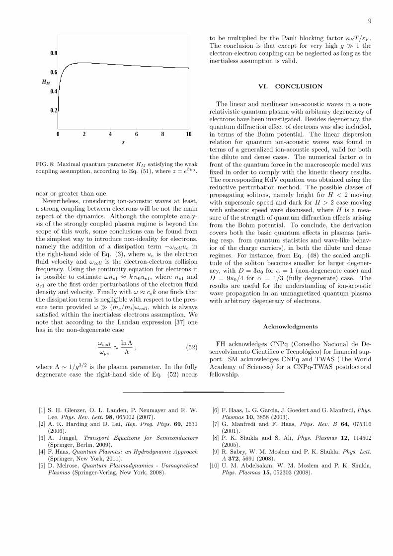
On the other hand, it is interesting to examine theconditions for weak coupling as deduced in the presenttheory. Combining the weak coupling condition yieldingthe minimal temperature in Eq. (17) with Eq. (49) givesan upper bound on the quantum diffraction parameter,or

H2 < H2M ≡ −

(3

π

)1/3 Li−1/2(−eβµ0)Li5/2(−eβµ0)

[Li23/2(−eβµ0)]2/3,

(51)which is shown in Fig. (8). It follows that large H > 2values fall within the strongly coupled regime where cou-pling parameter g for degenerate electrons may become

9

0 2 4 6 8 10

0.2

0.4

0.6

0.8

z

HM

FIG. 8: Maximal quantum parameter HM satisfying the weakcoupling assumption, according to Eq. (51), where z = eβµ0 .

near or greater than one.Nevertheless, considering ion-acoustic waves at least,

a strong coupling between electrons will be not the mainaspect of the dynamics. Although the complete analy-sis of the strongly coupled plasma regime is beyond thescope of this work, some conclusions can be found fromthe simplest way to introduce non-ideality for electrons,namely the addition of a dissipation term −ωcollue inthe right-hand side of Eq. (3), where ue is the electronfluid velocity and ωcoll is the electron-electron collisionfrequency. Using the continuity equation for electrons itis possible to estimate ωne1 ≈ k n0ue1, where ne1 andue1 are the first-order perturbations of the electron fluiddensity and velocity. Finally with ω ≈ csk one finds thatthe dissipation term is negligible with respect to the pres-sure term provided ω � (me/mi)ωcoll, which is alwayssatisfied within the inertialess electrons assumption. Wenote that according to the Landau expression [37] onehas in the non-degenerate case

ωcollωpe

≈ ln Λ

Λ, (52)

where Λ ∼ 1/g3/2 is the plasma parameter. In the fullydegenerate case the right-hand side of Eq. (52) needs

to be multiplied by the Pauli blocking factor κBT/εF .The conclusion is that except for very high g � 1 theelectron-electron coupling can be neglected as long as theinertialess assumption is valid.

VI. CONCLUSION

The linear and nonlinear ion-acoustic waves in a non-relativistic quantum plasma with arbitrary degeneracy ofelectrons have been investigated. Besides degeneracy, thequantum diffraction effect of electrons was also included,in terms of the Bohm potential. The linear dispersionrelation for quantum ion-acoustic waves was found interms of a generalized ion-acoustic speed, valid for boththe dilute and dense cases. The numerical factor α infront of the quantum force in the macroscopic model wasfixed in order to comply with the kinetic theory results.The corresponding KdV equation was obtained using thereductive perturbation method. The possible classes ofpropagating solitons, namely bright for H < 2 movingwith supersonic speed and dark for H > 2 case movingwith subsonic speed were discussed, where H is a mea-sure of the strength of quantum diffraction effects arisingfrom the Bohm potential. To conclude, the derivationcovers both the basic quantum effects in plasmas (aris-ing resp. from quantum statistics and wave-like behav-ior of the charge carriers), in both the dilute and denseregimes. For instance, from Eq. (48) the scaled ampli-tude of the soliton becomes smaller for larger degener-acy, with D = 3u0 for α = 1 (non-degenerate case) andD = 9u0/4 for α = 1/3 (fully degenerate) case. Theresults are useful for the understanding of ion-acousticwave propagation in an unmagnetized quantum plasmawith arbitrary degeneracy of electrons.

Acknowledgments

FH acknowledges CNPq (Conselho Nacional de De-senvolvimento Cientıfico e Tecnologico) for financial sup-port. SM acknowledges CNPq and TWAS (The WorldAcademy of Sciences) for a CNPq-TWAS postdoctoralfellowship.

[1] S. H. Glenzer, O. L. Landen, P. Neumayer and R. W.Lee, Phys. Rev. Lett. 98, 065002 (2007).

[2] A. K. Harding and D. Lai, Rep. Prog. Phys. 69, 2631(2006).

[3] A. Jungel, Transport Equations for Semiconductors(Springer, Berlin, 2009).

[4] F. Haas, Quantum Plasmas: an Hydrodynamic Approach(Springer, New York, 2011).

[5] D. Melrose, Quantum Plasmadynamics - UnmagnetizedPlasmas (Springer-Verlag, New York, 2008).

[6] F. Haas, L. G. Garcia, J. Goedert and G. Manfredi, Phys.Plasmas 10, 3858 (2003).

[7] G. Manfredi and F. Haas, Phys. Rev. B 64, 075316(2001).

[8] P. K. Shukla and S. Ali, Phys. Plasmas 12, 114502(2005).

[9] R. Sabry, W. M. Moslem and P. K. Shukla, Phys. Lett.A 372, 5691 (2008).

[10] U. M. Abdelsalam, W. M. Moslem and P. K. Shukla,Phys. Plasmas 15, 052303 (2008).

10

[11] A. E. Dubinov and A. A. Dubinova, Plasma Phys. Rep.33, 859 (2007).

[12] S. Mahmood and F. Haas, Phys. Plasmas 21, 102308(2014).

[13] A. E. Dubinov and A. A. Dubinova, Plasma Phys. Rep.34, 403 (2008).

[14] G. Manfredi and J. Hurst, Plasma Phys. Control. Fusion57, 054004 (2015).

[15] J. E. Cross, B. Reville and G. Gregori, Astrophys. J. 795,59 (2014).

[16] N. Maafa, Phys. Scripta 48, 351 (1993).[17] B. Eliasson and P.K. Shukla, J. Plasma Phys. 76, 7

(2010).[18] A. Mushtaq and D. B. Melrose, Phys. Plasmas 16,

102110 (2009).[19] D. B. Melrose and A. Mushtaq, Phys, Rev. E 82, 056402

(2010).[20] B. Eliasson and P. K. Shukla, Phys. Scripta 78, 025503

(2008).[21] A. E. Dubinov, A. A. Dubinova and M. A. Sazokin, J.

Commun. Tech. Elec. 55, 907 (2010).[22] J. R. Barker and D. K. Ferry, Semicond. Sci. Technol.

13, A135 (1998).[23] C. L. Gardner, SIAM J. Appl. Math. 54, 409 (1994).[24] H. L. Rubin, T. R. Govindan, J. P. Kreskovski and M.

A. Stroscio, Solid St. Electron. 36, 1697 (1993).[25] R. K. Pathria and P. D. Beale, Statistical Mechanics -

3rd ed. (Elsevier, New York, 2011).[26] L. Lewin, Polylogarithms and Associated Functions

(North Holland, New York, 1981).[27] A. I. Akhiezer, I. A. Akhiezer, R. V. Polovin, A. G.

Sitenko and K. N. Stepanov, Plasma Electrodynamics -vol. I (Pergamon, Oxford, 1975).

[28] J. Zamanian, M. Marklund and G. Brodin, New J. Phys12, 043019 (2010).

[29] P. K. Shukla and B. Eliasson, Rev. Mod. Phys. 83,885(2011).

[30] A. P. Misra and P. K. Shukla, Phys. Rev. E 85, 026409(2012).

[31] D. Michta, F. Graziani and M. Bonitz, Contrib. PlasmaPhys. 55, 437 (2015).

[32] M. Akbari-Moghanjoughi, Phys. Plasmas 22, 022103(2015).

[33] D. Bohm and D. Pines, Phys. Rev. 92, 609 (1953).[34] R. C. Davidson, Methods in Nonlinear Plasma Theory

(Academic Press, New York, 1972).[35] T. Kawahara, Phys. Soc. Japan 33, 260 (1972).[36] V. Yu. Belashov and S. V. Vladimirov, Solitary Waves

in Dispersive Complex Media (Springer-Verlag, Berlin-Heidelberg, 2005).

[37] E. M. Lifshitz and L. P. Pitaevskii, Physical Kinetics(Pergamon, Oxford, 1981).