linear and nonlinear acoustic wave propagation in … · 1. introduction linear and nonlinear...

NASA Contractor Report 4157

NASA-CR-4157 19880015884

Linear and Nonlinear

Acoustic Wave Propagation in the Atmosphere

s. I. Hariharan and Yu Ping

GRANT NAG 1-624 JUNE 1988

.,. "~ 'I. ... , -, -- ~i. _,.. ..

" ,

'- f :- I f 1) -'~ I 'or I, ",

, , r ' ... I •

N!\SI\ 111111111111111111111111111111111111111111111 NF01823

,--

https://ntrs.nasa.gov/search.jsp?R=19880015884 2018-08-18T21:33:52+00:00Z

3 1176013440087

NASA Contractor Report 4157

Linear and Nonlinear Acoustic Wave Propagation in the Atmosphere

s. I. Hariharan and Yu Ping University of Akron Akron, Ohio

Prepared for Langley Research Center under Grant NAG 1-624

NI\SI\ National Aeronautics and Space Administration

Scientific and Technical Information Division

1988

1. Introduction

Linear and Nonlinear Acoustic Wave Propagation in the Atmosphere

s. I. Hariharan*

Yu Ping**

Department of Mathematical Sciences University of Akron, Akron, OH 44325

In this paper we describe procedures for computing linear and nonlinear aspects of acoustic wave

propagation in the atmosphere. Acoustic waves originate from a source that has compact support in

space, as well as in time. Such a phenomena occurs in a situation such as shuttle take off or any general

explosion. The current work concentrates on a situation in which the atmosphere is isothermal.

Although this assumption somewhat over-simplifies the physics, the mathematical and computational

aspects of the problem remain difficult. The main difficulty arises from the effect of gravity, which is

included in this model and plays a crucial role in the nature of the propagation. In the acoustics litera

ture, similar models were used to investigate explosive waves. We cite references [1] and [2] where

linear models were considered for such purposes. Our model is an improvement over the model pro

posed in [1]. Our work appearing in [3] and [4] discuss analysis of the problem in two dimensions. Our

work appearing in [5] discusses the first computational effort in the three-dimensional situation but only

the linear case was discussed. The work reported in this paper includes numerical aspects of nonlineari

ties in the three-dimensional situation.

The main goal of this paper is to capture the effects of these atmospheric acoustic waves numeri

cally. While the goal seems to be simple, there are several obstacles in the process of solving the prob

lem under consideration. The nonlinear problem for the acoustic variables cannot be directly solved

with a reasonable computational effort unless the problem is somewhat simplified by some techniques.

In the sequence of work reported in [3] and [4] the nonlinear problem was reduced to a sequence

of linear problems using appropriate asymptotic expansions. Then one could show the linearized prob

lems were well-posed. There was a question that we could not resolve about the asymptotic expansion.

The expansion may not be uniformly valid. Here, we provide partial justification by considering an

appropriate one dimensional model. We compute the linearized solutions and show the sum of the first

two terms of the expansion yield indeed the solution of the nonlinear problem. Unfortunately, this can

*This work was supported by a grant from National Aeronautics and Space Administration, grant No. NAG -1 - 624, and in part by a National Science Foundation grant, grant No. DMS- 8604047. **Graduate Student.

- 2 -

be done only in a one-dimensional situation, as the cost of computing solutions of the nonlinear prob

lem directly is extremely high. This is because the actual nonlinear acoustic field contains the mean flow

fluid quantities which are orders of magnitude higher than the acoustic quantities. In particular, the

truncation error resulting from the numerical scheme will dominate the acoustic effect unless a very

fine grid and extremely small time steps are used. In the calculations reported on the one-dimensional

situation, 400 mesh points and about 10,000 time steps are needed to directly compute the nonlinear

problem. To carry out this procedure to higher dimensions, it is clear that one requires large computa

tional requirements. The justification for the validity of the asymptotic expansion that we provide here

is computational, and a mathematical proof is a hard task as pointed out in [3]; therefore we leave it as

an open question.

The plan of the paper is as follows. First, we shall present the governing equations and present

the problems that we intend to solve. In these problems, boundary conditions playa crucial role. The

boundary conditions that we use here are different from and better than the ones we used in [5]. The

derivations are not straightforward. They are presented in the appropriate sections. We devote section 2

of the paper to the discussion of the one-dimensional model where the problem can be reduced to a

scalar problem. In section 3, we discuss the sequence of linearized problems and in section 4, we dis

cuss the nonlinear system in the one-dimensional situation. In section 5, we discuss the axisymmetric

three-dimensional problem. We also show the numerical results in sections 3,4 and 5 arising from our

theory and computations. In section 6, we show the numerical schemes that we used for our computa

tions, along with the numerical treatment of our boundary conditions.

1.1 Governing Equations

We shall begin with the statement of the fluid flow problem that governs the acoustic phenomena.

If p. is the ambient pressure and h is the scale height, then the non-dimensional form of the Euler

equations (the equations of continuity, balance of momentum, and energy) are * + div(pq) = 0, ( 1.1)

~ + (q. V)q= __ I_Vji _ 1.k, at 'YP 'Y

(1.2)

[ a }f, 1 -a +q'V =---=tef(x,y,z,t). t p'Y p'Y

( 1.3)

Note that, in equation (1.2), the forcing term - 1 k (k is the unit vector in the z direction) arises due 'Y

to the forcing term per unit mass - gk in the original variables which is due to gravity. In equation

(1.3), f (x ,y ,z ,t) dictates the space-time dependency of the source, and e measures the energy release

per unit volume. For the case of an instantaneous energy release, e is given by

- 3 -

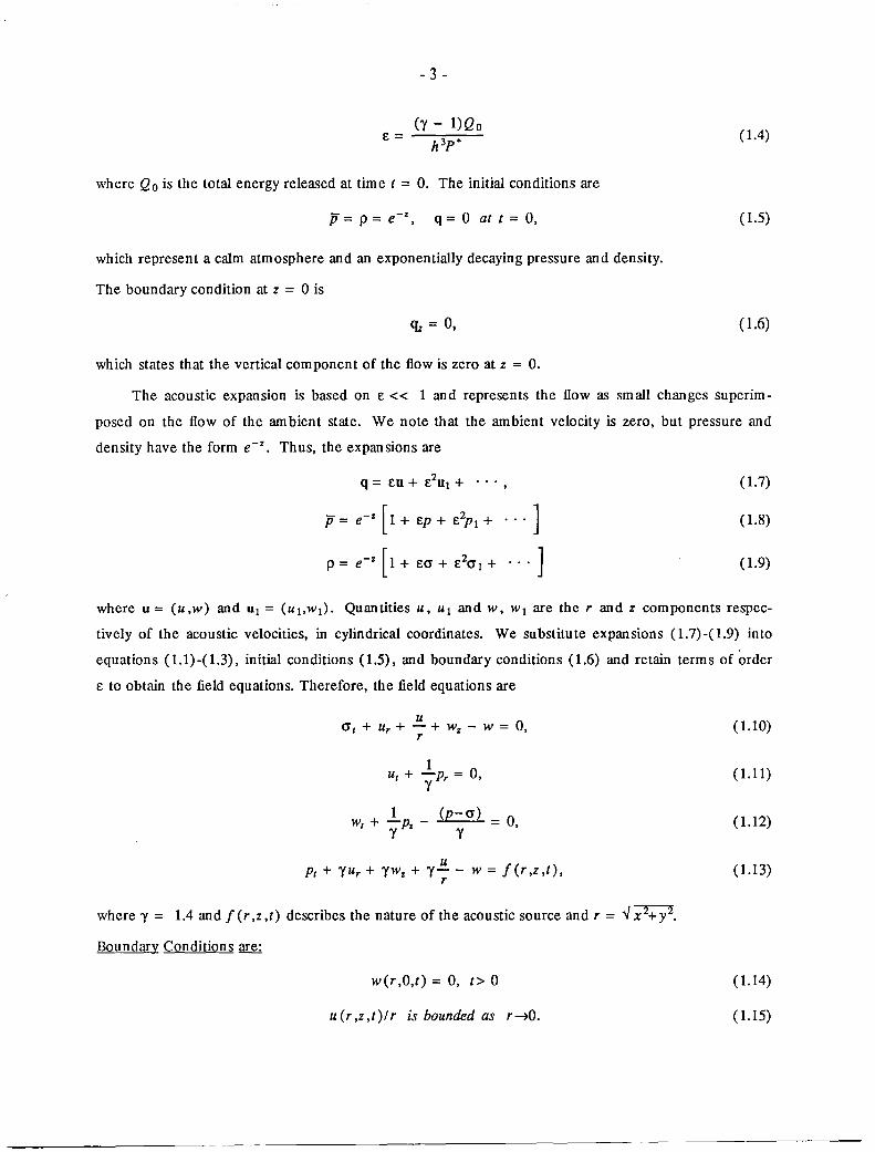
e= (1.4)

where Qo is the total energy released at time t = 0. The initial conditions are

fi = P = e- z, q = ° at t = 0, ( 1.5)

which represent a calm atmosphere and an exponentially decaying pressure and density.

The boundary condition at z = ° is

<Iz = 0, ( 1.6)

which states that the vertical component of the flow is zero at z = 0.

The acoustic expansion is based on e« 1 and represents the flow as small changes superim-

posed on the flow of the ambient state. We note that the ambient velocity is zero, but pressure and

density have the form e- z • Thus, the expansions are

q = eu + e2ul + ( 1.7)

fi = e- z [ 1 + ep + e2pl + ... ] ( 1.8)

p = e- z [1 + eO' + e20'1 + ... ] ( 1.9)

where U = (u,w) and UI = (UloWI)' Quantities u, UI and w, WI are the r and z components respec

tively of the acoustic velocities, in cylindrical coordinates. We su bstitu te expan sions (1.7) -( 1.9) into

equations (1.1)-( 1.3), initial conditions (1.5), and boundary conditions (1.6) and retain terms of order

e to obtain the field equations. Therefore, the field equations are

U 0' t + Ur + - + Wz - W = 0,

r

1 ut + -Pr = 0,

Y

W + ..!.p - (p-O') = 0, t Y Z Y

U Pt + YUr + ywz + Y- - W = f(r,z,t),

r

where Y = 1.4 and f (r ,z ,t) describes the nature of the acoustic source and r = ...j x 2+ y2.

Boundary Conditions are:

w(r,O,t) = 0, t> 0

u(r,z,t)/r is bounded as r~O.

( 1.10)

(1.11)

( 1.12)

(1.13)

(1.14)

( 1.15)

- 4 -

Initial Conditions are:

P = cr = U = W = 0 for t = O. ( 1.16)

In addition, we also need a radiation condition for the problem that describes the behavior of the wave

at infinity. In this problem, a radiation condition must be included for the uniqueness of the solution.

The condition here is that the waves decay at infinity and, when imposed at finite distances, take the

form

1 (u - yp), 1 U

W - -w + at r Z y r R, (1.17a)

1 1 1 U (w - -p)t = -(p - cr) - (-w - ur ) at z = L.

Y Y Y r ( 1.17b)

The derivation is based on [8] and is given in section 5.

We shall denote the problem formed by equations (1.10) - (1.17) by (P). Our procedure advo

cated in [3), as well as in [4), is to solve for the next correction and add the correction to the solution

of (P) to obtain the solution of the nonlinear problem. In this process, the equations governed by the

next order terms contain exactly the same differential operator, except the right hand side contains the

solution of problem (P). We call the the resulting problem of the next order to be (P') and is as fol

lows:

UI crl t + ulr + - + Wlz - WI = flo r

1 u1I + yPlr = 12,

UI PIt + yUlr + YWlz + Y- - WI = 14, r

where fl. f 2. f 3 and f 4 contain solution of the problem (P) and given by

f I = - [(cru)r + (crw)z - cr(w - E..»), r

1 f 2 = -crpr - (UUr + WU Z ),

Y

1 1 h = - [uwr + WWz + -cr(p - cr)] + -crpz, Y Y

U f 4 = crf + pew - Y-) - yp(ur + Wz) - (uPr + wpz). r

( 1.18)

( 1.19)

( 1.20)

( 1.21)

- 5 -

The boundary and initial conditions have the same form as before and are given below.

Boundary Conditions are:

WI(r,O,t) = 0, t > 0,

uI(r,z,t)lr is bounded as r~O.

Initial Conditions are:

PI = 0'1 = UI = WI = 0 for t = O.

The radiation condition takes the form

1 1 UI 1 (UI - yPI)t = -(-Wlz + yWI - -;-) + yO'Pr - UUr

1 U - WUz + -[p(w-Y-) - yp(ur + wz) - (uPr + wpz)] at r = R,

Y r

(1.22)

( 1.23)

(1.24)

(1.25a)

1 Ul 1 1 1 = - y(WI - r--;: - rUlr ) + y(PI - al) + yapZ - [uwr + WWz + ya(p - 0')]

1 U 1 - -p(w - Y-) + p(ur + wz) + -(uPr + wpz) at z = L.

Y r Y (1.25b)

It is shown in [3] and [5], these linearized problems are well-posed. However, it remains to be deter

mined if the expansions proposed in equations (1.6) - (1.8) are uniformly valid. If they are, then we

have a justification to assume that the full nonlinear problem is well-posed in the sense of the results

reported in [3] and [5]. To demonstrate the validity of the asymptotic expansion, we consider a

sequence of one-dimensional models. We show that the resulting linear problems from the asymptotic

expansions indeed lead to the solution of the original nonlinear problem. At the outset, let us

emphasize that even the linear one-dimensional problem does not have a closed form solution. For this

reason, we solve the problem in two essentially different ways to reach an agreement in the solution

that we obtain through numerical methods. In the next section, we reduce the problem to one that is

governed by a scalar wave equation. While the field equations become simple, the formulation of the

radiation condition becomes a laborious task. The derivation is included. In section three, we consider

the linearized systems. In section four, we solve the nonlinear equation. Numerical methods and

derivation of the boundary conditions are included. Here we compare the results obtained in the

preceding two sections. In section five, we solve the three-dimensional axisymmetric model. Again, the

boundary conditions are paid special attention. Also, we formulate the problem in the absence of grav

ity and show the derivation of appropriate nonreflecting conditions. We solve this problem and compare

the effect of gravitation with the solution obtained from the original systems. In section six, we con

clude the paper with the numerical methods that we used.

- 6 -

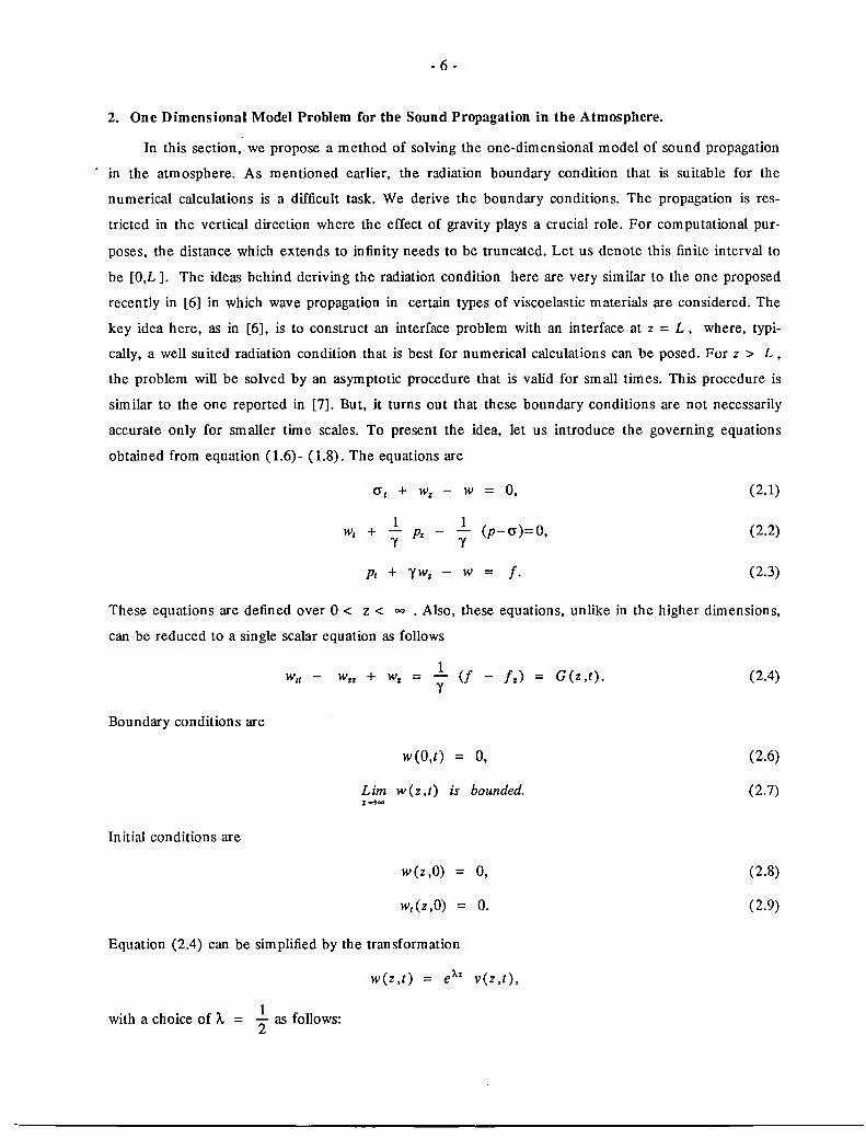
2. One Dimensional Model Problem for the Sound Propagation in the Atmosphere.

In this section, we propose a method of solving the one-dimensional model of sound propagation

in the atmosphere. As mentioned earlier, the radiation boundary condition that is suitable for the

numerical calculations is a difficult task. We derive the boundary conditions. The propagation is res

tricted in the vertical direction where the effect of gravity plays a crucial role. For computational pur

poses, the distance which extends to infinity needs to be truncated. Let us denote this finite interval to

be [O,L]. The ideas behind deriving the radiation condition here are very similar to the one proposed

recently in [6] in which wave propagation in certain types of viscoelastic materials are considered. The

key idea here, as in [6], is to construct an interface problem with an interface at z = L, where, typi

cally, a well suited radiation condition that is best for numerical calculations can be posed. For z > L,

the problem will be solved by an asymptotic procedure that is valid for small times. This procedure is

similar to the one reported in [7]. But, it turns out that these boundary conditions are not necessarily

accurate only for smaller time scales. To present the idea, let us introduce the governing equations

obtained from equation (1.6) - (1.8). The equations are

crt + Wz - W = 0, (2.1)

1 1 (p-cr)=O, (2.2) W t + - pz - -

y y

Pt + YWz - W = I· (2.3)

These equations are defined over ° < z < 00 • Also, these equations, unlike in the higher dimensions,

can be reduced to a single scalar equation as follows

Wit -1

Wzz + Wz = - (f - Iz) Y

Boundary conditions are

W(O,t) = 0,

Lim w(z,t) is bounded. Z-4~

Initial conditions are

W(z ,0) = 0,

Wt(z ,0) = 0.

Equation (2.4) can be simplified by the transformation

W(z ,t) = e AZ v(z ,t),

with a choice of A 1 "2 as follows:

G(z,t). (2.4)

(2.6)

(2.7)

(2.8)

(2.9)

- 7 -

1 --z e 2 G(z,t) = g(z,t). (2.10)

Suppose we want to impose boundary condition, exact or otherwise, at the finite distance L that

simulates the behavior at infinity. We claim that these boundary conditions are of the form

Vz = Bv + Kg, (2.11)

where B and K are operators to be determined. In the event that g has a compact support in

o < z < L, the boundary condition will take the form

Vz = Bv. (2.12)

2.1 Procedure

Initial conditions suggest that we consider the problem in the Laplace transform domain. Doing

so, we obtain

1 A A

-v + g. 4

(2.13)

Here v lows

v(z ,s) and g g(z ,s). The main theme here is to consider an interface problem as fol-

1 vtt = vzz - 4"v + g(z ,t), 0< z < L,

which is the given field equation. Now define O'(z,s;t) such that

S2UA

= UA

1 UA

() zz - 4" + g z ,t , z> L,

with

O'(L,s;t) = v(L,t).

We remark that here t is considered as a parameter. Now it is easily verified that

v(z,s) = J e-stO'(z,s;t)dt. o

(2.14)

(2.15)

(2.16)

(2.17)

The plan here is to solve equation (2.15) subject to the interface condition (2.16) and a radiation

condition which insures the boundedness of v(z ,t) , which translates in the transform domain to

requiring the boundedness of 0' (z ,s;t). As mentioned earlier, our procedure for constructing the solu

tion will be an asymptotic one with s as a parameter and for large s, reflecting the fact that solutions

will be accurate for smaller times. However, asymptotic methods are known for their power. Even

though the expansion is valid for small time in the theoretical treatment, need not be small for real

- 8 -

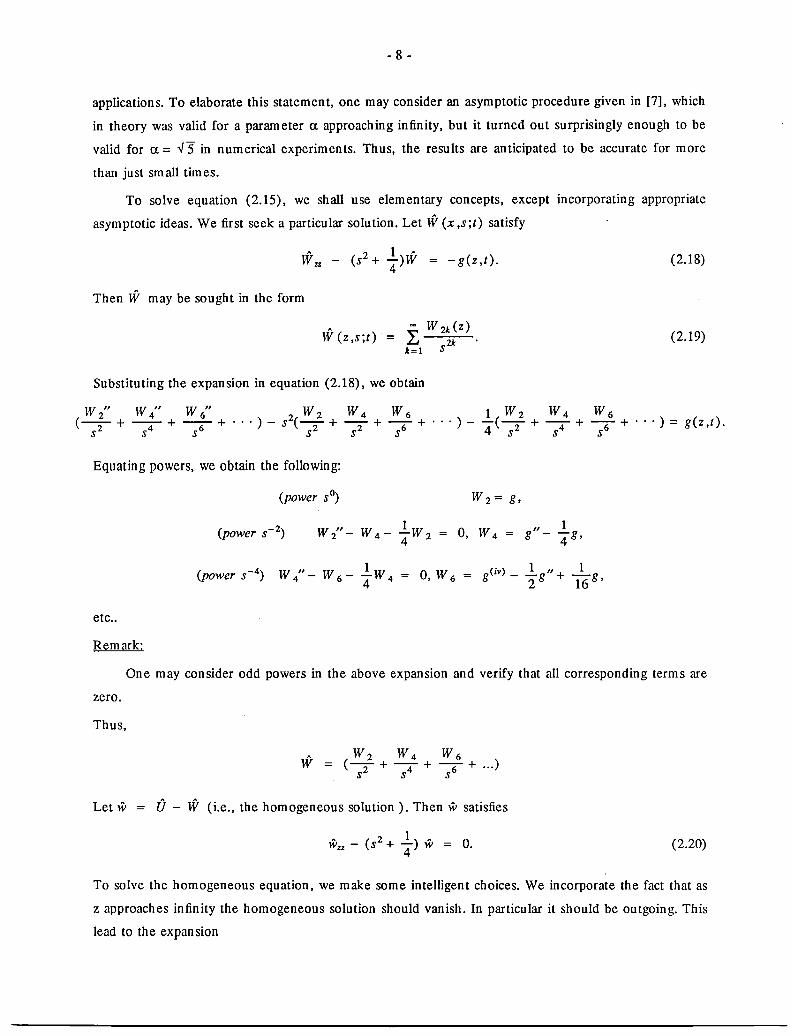
applications. To elaborate this statement, one may consider an asymptotic procedure given in [7], which

in theory was valid for a parameter (l approaching infinity, but it turned out surprisingly enough to be

valid for (l = ..J5 in numerical experiments. Thus, the results are anticipated to be accurate for more

than just sm all tim es.

To solve equation (2.15), we shall use elementary concepts, except incorporating appropriate

asymptotic ideas. We first seek a particular solution. Let W (x ,s;t) satisfy

Wzz

Then W may be sought in the form

2 1 A

(s + "4)W -g(z,t).

W (z ,s;t) = ~ W 2k (z)

.LJ 2k • 1=1 S

Substituting the expansion in equation (2.18), we obtain

(2.18)

(2.19)

W 2" W 4" W 6" 2 W 2 W 4 W 6 1 W 2 W 4 W 6 (-- + -- + -- + ... ) - s (- + - + - + ... ) - -(- + - + - + ... ) = g(z,t).

S2 S4 S6 S2 s2 S6 4 S2 S4 S6

Equating powers, we obtain the following:

etc ..

Remark:

1 W 2"- W 4 - "4W2

1 W 4" - W 6 - - W 4

4 0, W6

W 2 = g,

0, W 4 = g"

g (iv) _ 1" 1 2: g + 16g ,

One may consider odd powers in the above expansion and verify that all corresponding terms are

zero.

Thus,

W 2 W 4 W6 (-2 + -4 + -6 + ... )

S S S

Let w (] - W (i.e., the homogeneous solution ). Then w satisfies

A (2 I)A 0 Wzz - S +"4 W = . (2.20)

To solve the homogeneous equation, we make some intelligent choices. We incorporate the fact that as

z approaches infinity the homogeneous solution should vanish. In particular it should be outgoing. This

lead to the expansion

- 9 -

U U W = e-s(z-L)(U O+ _1 + _2+ "').

S S2 (2.21)

Su bstitu ting the above expan sion in equation (2.20), we have

U' U' U" U" 1 U U -2s(U 0' + _1 + --T- + .... ) + (U 0" + _1_ + -+ + ... ) - -4 (U 0 + _1 + -+ + ... ) O.

s s s s s s

Recall that w = U - W. We also have the requirement that U(L ,s;t) = v(L ,t). Thus,

w(L ,s;t) = v(L ,t) - W (L ,s;t), indicating that the first term independent of s on the right is

v(L ,t). Using this fact in the previous expansion (2.21) and by equating the sl powers, we obtain

U o'= 0; Uo(L,t) = constant; Uo(L,t) = v(L,t).

The next term we obtain in the expansion is

2U ' U " 1 U 0 - 1+ 0-"40=.

Again we note that at z = L the right hand side of w = U - W does not have inverse power of

s, yielding U I(L ,t) = O. Thus, integrating for U 10 we get

1 U I(Z;t) = -iv(L ,t) (z-L)

The next term in the expansion has some interesting features. This time, forcing terms will appear in

the expansion. When doing the expansion, we find that

We see as before from the construction of w that

U 2(L,t) = -W2 = -g(z,t).

Thus, integration yields

1 ( 2 U 2 = 128 vL ,t)(z-L)-g

A similar procedure yields

1 1 3 U 3 = 128 v(L ,t)(z-L) - 3182 v(L ,t)(z-L) - g"(z-L).

We note here that on the boundary z = L , U 3 = O. Moreover, the remaining terms in the

expansion, when evaluated at z = L, yield only terms involving g and its derivatives. Thus summar

izing the results, we have

U (z ,s;t) ... ) + .... (2.22)

- 10 -

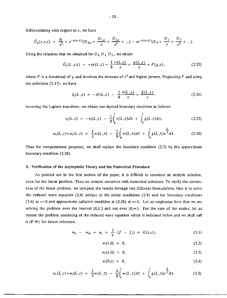
Differentiating with respect to z, we have

Uz(Z,s;t) = g; + e-s(z-L)(Uo,z + U 1,z + u~z + ... ) _ se-s(x-L)(U o + U 1 + u; + ... ). s s s s s

Using the relations that we obtained for U 0, U 1, U 2, we obtain

U~ (L .) = _ (L ) _.! v(L,t) g(L,t) ( z ,s,t SV ,t 8 + +Fg,s),

s s (2.23)

where F is a functional of g and involves the inverses of s4 and higher powers. Neglecting F and using

the definition (2.17), we have

(2.24)

Inverting the Laplace transform, we obtain our desired boundary condition as follows:

I I

vz(L ,t) = -v/(L ,t) - ! J v(L ,'t)d't + J g(L ,'t)d't, o 0

(2.25)

I I L

wz(L ,t)+w/(L ,t) 1

'2w(L ,'t) !J w(L,'t)d't + f g(L,'t)e 2 d't. o 0

(2.26)

Thus for computational purposes, we shall replace the boundary condition (2.7) by the approximate

boundary condition (2.26).

3. Verification of the Asymptotic Theory and the Numerical Procedure

As pointed out in the first section of the paper, it is difficult to construct an analytic solution,

even for the linear problem. Thus we content ourselves with numerical solutions. To verify the correct

ness of tne linear problem, we compute the results through two different formulations. One is to solve

the reduced wave equation (2.6) subject to the initial conditions (2.8) and the boundary conditions

(2.6) at z=O and approximate radiative condition at (2.26) at z=L. Let us emphasize here that we are

solving the problem over the interval [O,L] and not over [0,00). For the ease of the reader, let us

restate the problem consisting of the reduced wave equation which is indicated below and we shall call

it (P-W) for future reference.

w"~ - Wzz + Wz = ~ (f - f z) G(z,t),

W(z ,0) = 0,

W,(z,O) 0,

W(O,t) 0,

I I L

wz(L,t)+w,(L,t) = ~w(L,'t) - !J w(L,'t)d't + J g(L,'t)e 2 d't. o 0

(3.1)

(3.2)

(3.3)

(3.4)

(3.5)

- 11 -

Solving (P-W) numerically is straight-forward. It is solved by an explicit finite difference formula.

This is a standard discretization. The integrals in the boundary condition (3.5) are evaluated by a rec

tangular quadrature formula. It could be shown that problem (P-W) is well-posed in the sense of a

bounded growth of energy. Related ideas can be found in MacCamy [6]. However, the situation here is

different and the related theoretical results will be reported elsewhere.

As mentioned earlier, the comparison could be made by solving the system (2.1) - (2.3) with

appropriate initial and boundary conditions as described in the last section. Still the problem is to be

considered in the truncated domain [O,L J. However, the system involves the primitive variables for the

acoustic components p, p and w. The boundary condition (2.26) thus need to be recast in these vari

ables in an appropriate manner which is suitable for numerical computations. Again, we summarize the

equations that we wish to solve.

cr, + Wz - w = 0 (3.6)

1 1 w, + y pz - y (p-cr)=O (3.7)

p, + YWz - w f (3.8)

The initial conditions are

p cr = w = 0 (at t = 0). (3.9)

The boundary conditions are

w(O,t) = 0 (3.10)

and (3.5). We replace Wz in (3.5) using equation (3.8) so that the left side of the boundary operator

becomes the rate of change of incoming Riemann variable. The result is

a -(p - yw) at

, , L

(1- t) w + f + if w(L,'t)d't - yI g(L,'t)e2 d't. o 0

(3.11)

We shall call the problem (3.6) - (3.11) by (P-Ll). We briefly show the calculations that identify the

Riemann variables associated with the system. First, we note that that the system (3.6) - (3.8) can be

written in the form

with

u, + Auz = H

uT = (cr, w ,p),

1 = (w,-(p - cr),w + f),

y

(3.12)

(3.13)

(3.14)

- 12 -

and

It is easily shown that the eigenvalues of A are (1,-1,0). Corresponding left eigenvectors are

e2 (O,-y ,1)T,

e3 (-y ,0,1)T.

Multiplying on the left of (3.12) by each of these vectors, we obtain

R,+R z = w+p-O"+/,

s, - Sz w - p + 0" + / ,

T, = w - yw + /.

Here

R = P + yw

and

S = p - yw,

(3.15)

(3.16)

(3.17)

(3.18)

are the outgoing and incoming Riemann variables respectively. T = p - y s carries no information, as

it has zero speed. These variables playa crucial role in the numerical implementation of boundary con

ditions. For example, when we implement the boundary condition (3.11), S is determined at the

current time level. However, to obtain the value of p and w, we use equation (3.16) (discretizations

may be seen in section 6.). This determines R . Once R and S are determined, p is determined by

R + S (z L ), p = = 2 (3.19)

R - S (z L ). w = 2y

(3.20)

A similar consideration is given at z = 0, where w = 0. To determine p, one can use equation

(3.17) for S. Once S is determined at z = 0, one immediately obtains

p = S (z = 0). (3.21)

Figures 1. and 2. show a comparison of the results obtained through solving the problems (P-W)

and (P-Ll) numerically. For the test case presented here, the source function / was chosen to have a

- 13 -

compact support in space and time as follows:

{

-a(. - '0>2 e sin 21t t

f(z,t) = 0 O:s; t:S; T, Iz - zol < £

otherwise. (3.22)

Here a = 40, Zo = 0.25L, £ = 0.025L and T = 1. The results are the same. The results shown

here are after 1000 and 7000 time steps, respectively, and the pressure distributions are shown in Fig

ures 1. and 2. In Figure 2., there is a little difference which is due the boundary conditions. However,

the scale is small and the difference is below the truncation error. Thus, with this agreement, we con

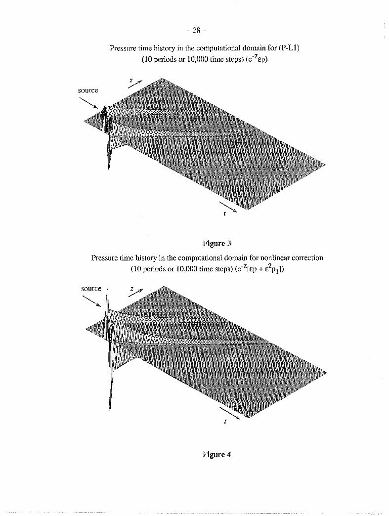
tend that the results are nearly equal to the analytic solution of the problem. In Figure 3, we show the

behavior of the pressure wave as a function of both space and time and time reaching up to 10,000

steps or 10 periods. We see that the wave moves in two directions: one towards the radiation boundary

and the other towards the ground. As one should expect, the wave that hits the ground reflects at

z = 0, and, eventually, all decay to zero. In the calculations reported here, ~z = 0.025, L = 10,

and the perturbation parameter £ = 0.005. There were 400 grid points used for the computations, indi

cating a fine grid. Thus, the results that we obtained here had to be thought of as exact.

3.1 Nonlinear Correction and the Fully Nonlinear Solution

Now we proceed to investigate the nonlinear effects. First, we propose a second-order correction

to the linear problem. This problem results by retaining 0(£2) terms as in equations (1.18) - (1.21).

These equations are

alt + Wlz - WI = -Caw). + aw = f 1> (3.23)

(3.24)

PIt + yWlz - WI = af + aw - ypwz + ywwt = f 3· (3.25)

Initial conditions are

PI = al = WI = 0 for t = O. (3.26)

The boundary condition at z 0 is

Wl(O,t) = 0, t > O. (3.27)

The radiation boundary condition at z = L has the same form as before, which is

(3.28)

- 14 -

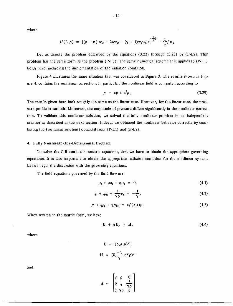
where

-.lL 1 H(L ,'t) = [(p - 0') Wzz - 2wwzt - (y + l)wz wt ]e 2 - r/O'Z.

Let us denote the problem described by the equations (3.23) through (3.28) by (P-L2). This

problem has the same form as the problem (P-L1). The same numerical scheme that applies to (P-Ll)

holds here, including the implementation of the radiation condition.

Figure 4 illustrates the same situation that was considered in Figure 3. The results shown in Fig

ure 4. contains the nonlinear correction. In particular, the nonlinear field is computed according to

(3.29)

The results given here look roughly the same as the linear case. However, for the linear case, the pres

sure profile is smooth. Moreover, the amplitude of pressure differs significantly in the nonlinear correc

tion. To validate this nonlinear solution, we solved the fully nonlinear problem in an independent

manner as described in the next section. Indeed, we obtained the nonlinear behavior correctly by com

bining the two linear solutions obtained from (P-Ll) and (P-L2).

4. Fully Nonlinear One-Dimensional Problem

To solve the full nonlinear acoustic equations, first we have to obtain the appropriate governing

equations. It is also important to obtain the appropriate radiation condition for the nonlinear system.

Let us begin the discussion with the governing equations.

The field equations governed by the fluid flow are

Pt + pqz + q P. = 0,

1 qt + qq. + -PI = yp

1

Y

Pt + qpz + ypqz el (z ,t)p.

When written in the matrix form, we have

where

and

U t + AUz = H,

U = (p,q ,p)T,

-1 T H = (O,-,el p) y

(4.1)

(4.2)

(4.3)

(4.4)

- 15 -

The eigenvalues of A are A. = q + ~ :-' q - ~ :- and q. Left eigenvectors corresponding to

these eigenvalues are

el = (O,y"pp,l)T,

e2 = (O,-y" pp,l)T,

respectively. Multiplying equation (4.4) by el , e2 and e3 we respectfully obtain the following equations:

(y,J pp,!) ~l + (q + ,j ;)(y,JpP,!) [~l = (y,J pp,!) [~p} 1

(-y,Jpp,!) ~l + (q - ,j ;)(-y,JpP,!) [~l = (-y,Jpp,l) [~p} 1 (1,-~) [ql + q (I,-~) [ql = -eL .

yp p yp p yp

(4.5a)

,(4.5b)

(4.6)

For sources that have a compact support as described in the numerical experiments earlier, equation

(4.3) suggests along a stream line that

where

P =Ap'Y,

Po A =

.(4.7)

With the above equations we can describe the fully nonlinear acoustic field and the associated radiation

conditions. Let

q = u'.

Thus, rewriting equation (4.4) in terms of the acoustic variables and dropping the "prime" notations, we

obtain the field equations in the matrix form as follows:

[pI [u (1 + p) u + 0 U

P 0 y(1 + p)

o 1

y(I + p) u

[

u (1 + p) 1 p-p y(I+p)

u(I + p) + ef(I + p)

(4.8)

- 16 -

These equations are to be solved subject to the initial conditions

p = p = u = 0 at t = 0, (4.9)

and boundary conditions

u = 0 at t = 0, (4.10)

and a radiation condition which we shall derive next at z = L.

When the above mentioned acoustic expansions are used in equations (4.5a) and (4.5b) together

with the isentropic relation (4.7), we obtain the following equations:

l.=.!. Ill.=.!. l.=.!. E _l.=.!. R t + (u + (l+p) 2y )R z = _- + -[u + (l+p) 2y ](I+p) 2y + !:L(1+p) 2y

y Y Y (4.11)

l.=.!. Ill.=.!. l.=.!. E _l.=.!. St + (u - (l+p) 2y )Sz = -y + y[u - (1+p) 2y ](1+p) 2y - 7(I+P) 2y (4.12)

and

1 + p (1 + p)Y. (4.14)

Here

2 L:....!. R = u + --(1 + p) 2y (4.15)

Y - 1

and

2 L=...!. S -u + --(1 + p) 2y • (4.16)

Y - 1

These variables as before in the linear case playa crucial role on the numerical, as well as physi

cal, boundary conditions. In this nonlinear situation, the boundary condition that we derived for the

linear case does not hold. Thus, we settle for a condition that is applicable for nonlinear problems

found in Thompson [9]. This is conceptually very simple once the equations are cast in the Riemann

variables. The principle here is that at z = L, for the waves not to reflect in the computational domain

the speed of the incoming variable must be zero. Thus, applying this condition in equation (4.12) for

the incoming variable, we obtain

1 1 L=...l L=...l E f _l.=.!. St = -- + -[u - (1 + p) 2y ](1 + p) 2y - -(1+p) 2y

Y Y Y ( 4.17)

This condition will be the replacing radiation condition for the nonlinear situation.

Numerical implementation of the system of equations (4.8) yields considerable problems. Even

though this is a hyperbolic system, it is not an integrable system. It cannot be cast in conservation or

- 17 -

weak conservation form. For these types of systems, numerical methods are not readily available in the

literature. Thus, we had to modify the Lax - Wendroffs method described in section 6. However, the

numerical treatment of the boundary conditions remain the same.

Again, the same test case that was applied to the linear system was simulated here. The source

was taken to be the same. The results are given in Figure 5. Comparing the results obtained in Figure

4., we see an excellent agreement between the combination of the two solutions of the linearized prob

lems and the full nonlinear solution. Again, we have used a surface plot to show the long time behavior

of the solution. We note in Figure 5. that there is a slight discrepancy in the results after a long time.

This is due to the inaccuracies in the nonlinear boundary condition (4.17). It should be noted once

again that these solutions were obtained from a fine grid (400 grid points) and to obtain the full non

linear problem in higher dimension can be tremendously costly. This is where the concept of solving

two successive linear problems becomes attractive. Indeed, we followed this principle to obtain the

three-dimensional axisymmetric problem which is discussed in the next section.

5. Three-Dimensional Axisymmetric Problem.

Here we consider the procedures for solving the three-dimensional problem. In particular, we

solve the problems (P) and (P') as described in section 1. The procedures for obtaining the radiation

boundary conditions are similar to that which we considered in the last section on the full one

dimensional nonlinear situation. The difficulty here is that the problem is multi-dimensional. Thus, for

the purpose of obtaining radiation conditions, we consider the Riemann variables in the direction where

we wish to impose the boundary condition. Let us consider the computational domain shown in Figure

6. Suppose on rlo which is located at r = R, we want to obtain appropriate radiation condition. We

apply the procedure described in section 4, by considering the system of equations only in the r direc

tion. The first two equations that we obtain are

R t + Rr 1 u = -wz + -w-'Y r

(5.1)

St - Sr 1 u = w - -w+ -z 'Y r

(5.2)

where

1 R = u + -p

'Y

and

1 S = u - -po

'Y

- 18 -

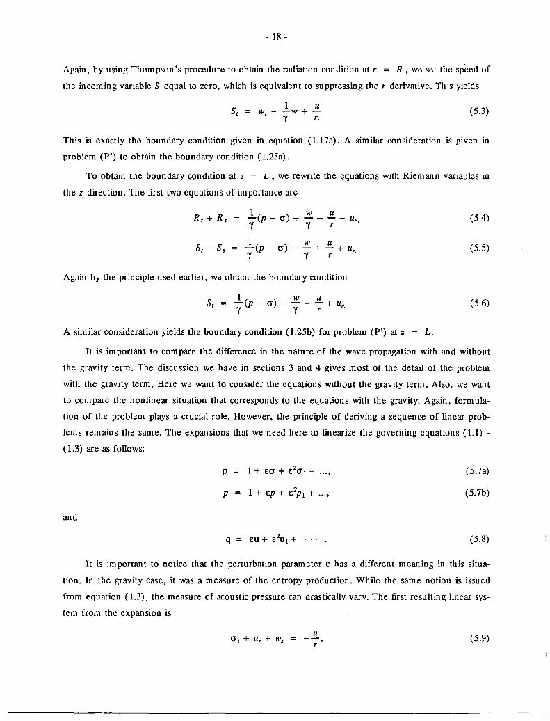
Again, by using Thompson's procedure to obtain the radiation condition at r = R, we set the speed of

the incoming variable S equal to zero, which is equivalent to suppressing the r derivative. This yields

St 1 U

w - -w + z 'Y r.

(5.3)

This is exactly the boundary condition given in equation (1.17a). A similar consideration is given in

problem (P') to obtain the boundary condition (1.25a).

To obtain the boundary condition at z = L, we rewrite the equations with Riemann variables in

the z direction. The first two equations of importance are

R t + R z 1 w U

(5.4) -(p - (1) + - - ur• 'Y 'Y r

St - Sz 1 w U

(5.5) = -(p - (1) - - + -+ Ur. 'Y 'Y r

Again by the principle used earlier, we obtain the boundary condition

1 w U S = -(p - (1) - - + - + U

t 'Y 'Y r r. (5.6)

A similar consideration yields the boundary condition (1.25b) for problem (P') at z = L.

It is important to compare the difference in the nature of the wave propagation with and without

the gravity term. The discussion we have in sections 3 and 4 gives most of the detail of the problem

with the gravity term. Here we want to consider the equations without the gravity term. Also, we want

to compare the nonlinear situation that corresponds to the equations with the gravity. Again, formula

tion of the problem plays a crucial role. However, the principle of deriving a sequence of linear prob

lems remains the same. The expansions that we need here to linearize the governing equations (1.1) -

(1.3) are as follows:

(5.7a)

(5.7b)

and

(5.8)

It is important to notice that the perturbation parameter e has a different meaning in this situa

tion. In the gravity case, it was a measure of the entropy production. While the same notion is issued

from equation (1.3), the measure of acoustic pressure can drastically vary. The first resulting linear sys

tem from the expansion is

u (5.9)

r

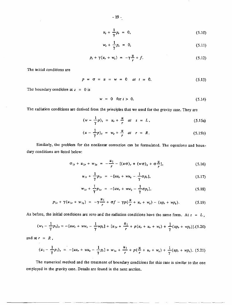
The initial conditions are

- 19 -

1 u, + -Pr = 0,

y

1 W, + -Pz = 0,

Y

U p, + y(ur + wz ) = -y- + f·

r

P = cr = U W = 0 at t = O.

The boundary condition at z = 0 is

W = 0 for t > O.

(5.10)

(5.11)

(5.12)

(5.13)

(5.14)

The radiation conditions are derived from the principles that we used for the gravity case. They are

1 U (w - -p), = U + - at z = L, Y r r (S.ISa)

1 U (u - -p), = W + - at r = R. Y z r (S.ISb)

Similarly, the problem for the nonlinear correction can be formulated. The equations and boun

dary conditions are listed below:

UI U = -- - [(ucr)r + (wcr)z + cr-],

r r

1 UI, + -Plr =

y

1 Wtt + -Ph

y

1 - [UUr + WUz - -crpr] ,

y

1 - [UWr + ww. - -crPz],

y

UI U PI, + y(Ulr + Wlz) = -y- + crf - yp(- + Ur + Wz) - (UPr + Wpz).

r r

(5.16)

(5.17)

(S.18)

(5.19)

As before, the initial conditions are zero and the radiation conditions have the same form. At z = L,

1 1 U I 1 (WI - -PI)' = - [UWr + WWz - -Wpz] + [Ulr + - + p(Ur + Ur + Wz) + -(UPr + wpz)].{S.20)

y y r y

and at r = R,

1 1 UI U 1 (UI - -y PI), = -[uur + wUz - -PrJ + Wiz + - + p(- + Ur + Wz ) + -(UPr + Wpz). (5.21) y r r y

The numerical method and the treatment of boundary conditions for this case is similar to the one

employed in the gravity case. Details are found in the next section.

- 20 -

5.1 Numerical Results and Discussions.

Numerical simulations are made by considering a pulse source above the ground which oscillates

sinusoidally for a finite time as before. The form is similar to the one that we used for the one dimen

sional simulation. It is

{

e-a(r- ro)2sin 21tt 0::;; t::;; T, Ir- rol < E

f(r,t) = 0 otherwise. (5.22)

Here, a = 20 and T = 1 and E = .005. Moreover, r = (r,z) and ro = (0,1). The time step was

chosen to be M = .01. Calculations were carried out up to 1300 steps or 13 periods.

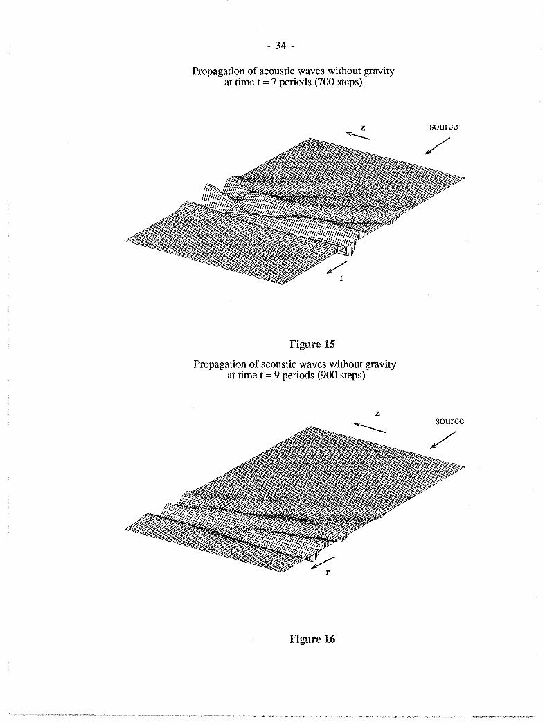
The results reported in this section are three-dimensional plots of pressure distribution over the

entire computational domain at different time intervals. The results reported in Figures 7 through 11

are the nonlinear solutions of the gravitational field equations. Each Figure shows the progress of the

wave at the end increment of one period. The results reported in Figures 12 through 16 correspond to

the same situation without the gravity term. As we see from these figures, the pressure field has higher

intensity in the absence of gravity than the case that includes gravity. However, after a long time the

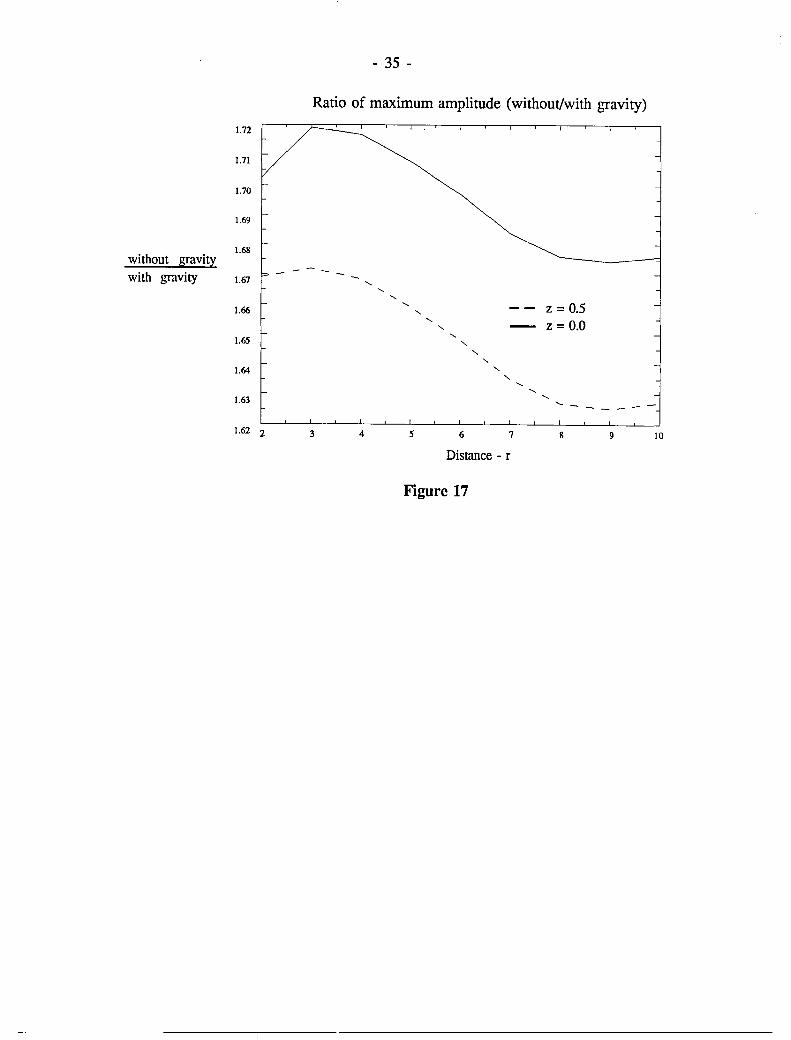
intensity of the gravitational field becomes higher. This is particularly true for large distances. Figure

17. shows the progression of the ratio of the maximum amplitude of the waves in each case. There are

two graphs, one is along the ground z = 0 (Solid line) and the other at z = 0.5 (dashed line). Ini

tially, the ratio of the pressure is higher for the no gravity case. As time progresses, the ratio decreases

and eventually the gravitational field begins to dominate. The nondimensional distances used here in

the z and r directions are 3 and 10 respectively. Since the lengths are nondimensionalized by the scale

height, the distance in the r direction is roughly 100 miles. Thus, in the gravitational field, the sound

tends to propagate longer distances, as suggested by our theory. Our computations are limited for such

short distances due to the cost in computations. The grid size was 75x250. To do more extensive calcu

lations, such as longer ranges, one requires a larger computational facility. The results reported here

took roughly 32 hours of computations on a SUN Microsystem Computer (3/260 - with floating point

accelerator). It took 15 minutes on a CRA Y - XMP-48. These considerations give a rough idea of the

large computational requirements of the problem.

A more realistic situation that could be considered is to include temperature variation and an

improved model of the atmosphere. A better atmospheric model validated with experiments are avail

able in [8]. We shall include this realistic model in a future continuation s>f this paper.

- 21 -

6. Numerical Schemes Used in the Computations.

Here we briefly describe the key numerical methods that we used in our computations. The cen

tral method is the well-known Lax-Wendroff method. In one dimensional conservative systems this

method is commonly known. For details, we refer to [10]. For nonconservative systems, the authors

are not aware of any extensions. Our extension that we used for the computations are presented. Also,

the multidimensional extensions that we used here and are not available in the literature are given here.

We begin with the one-dimensional scheme and the numerical evaluation of the Riemann variables

used to treat the boundary conditions.

6.1 Scheme for Linearized One-Dimensional Equation.

In this case, our equation takes the following form:

u t + F. = 8(u,z)

In the interior we use the Lax-Wendroff scheme, which is

U!+M I

At the boundary z = L ,the Riemann variables satisfy the following conditions:

St = Q(u),

Rt+R. = W (u).

The corresponding discretizations for these equations (see [11]), are

t+ At. S(uf/t.~ = S(u/.t) + S(U/.t_l) - S(u/.t~1~ + 2MQ(u 1)

N--2

O,I, ... N -1.

At z=O we have u=O, and we use the equation satisfied by S to obtain the numerical boundary

condition.

It should be pointed out that in the second order nonlinear correction, the right hand side of all

equations contain the derivatives of the first order problem. We evaluate these quantities using the fol

lowing formulas:

- 22 -

u l = (ul- u'_M )_I_

I !!. t

t+ .1! I+~ I-~ 1 ul 2 = (U 2 - U 2 )_

1 uf. = (Uf+l - utJ~

1+ .1! Uj. 2

6.2. Scheme for One-Dimensional Nonlinear Equations.

In this case, our equation takes the form

ul + A(u)F. = H(u)

M

As mentioned earlier, we modify the Lax-Wendroff scheme to obtain a numerical scheme. In the

event that A is linear, the scheme coincides with the Lax-Wendroff scheme.

it j+1 = ~ (Ul j+l + Ulj) i = O, ... N-l.

i=O, ... N-l

I+~ 1 1+ III 1+ III - 2 (2 2) Uj = "2 u. 1 + u. 1 0+"2 0-"2

1+.1! !!. t 1+ .1! 1+ .1! 1+ ~ ur"'l = uf + A(Uj 2 )-;--(F(u. ?) - F(u. ?)) + MH(Uj 2,Zj)

uZ 0+"2 0-"2 i = 1, ... N-l

6.3. Scheme for Linearized 3-D Equation.

In this case the equations have the form

Here again, we modify the Lax-Wendroff scheme. Our modification is similar to the Richtmyers

scheme given in [10]. Moreover, the equations are in the cylindrical coordinate system. Thus, there is a

singularity on the axis r= O. Our scheme and treatment of the singularity are given below:

".,.l 3 I 1 ( I I I I) U i j = '4u j 1 + 16 U i+l,j + U i-l,1 + u j,j+l + U j,j-l

- 23 -

i = 1, .. .N-l, j = 1,'" M-l

t+ III 1 - 2 (I -1+"1) U·· = - u .. + U· . '.} 2 '.} '.}

1+ Ill!l. .. U!i;M = U .. 2 _ _ t_(F(u!+tJ.~) _ F(u!+tJ.~))

',J '.} 2!l.z .+ 1,J .-1.}

~(G(U!i;M) - G(U!i;M)) + H(U!",:M r.)~ 2!l.r •. }+1 •• }-1 '.} '} 2 i = 1, . . . N - 1, j = 1, .. M - 1

At r=O there is a singularity. We evaluate the singular term using L'Hopitals rule as indicated

below:

u r

Then the scheme is modified at the origin by the following scheme:

(predictor step)

-t 3 1 1(1 I 21) U i.O = "4u i.O + 16 U i+l.0+U i-l.0 + U i.l

ul r i.O = :r uf.l

I 0.7 ( I I) 0.3 ( I I) U z i 0=-;:- Ui+l 0 - Ui-l 0 + -;:- Ui+ll - Ui-ll 'uZ ' • uZ f ,

uttM = uti 0 + !l.tX ti 0 . , ,

Wh X I xt (-I I I) ere i,O = i,O U i,O,ll r i,O,ll z i,O

( corrector step)

ul+M .l(u! + U!+M) i.O 2 •. 0 .,0

-u 1+ M _ 2 -1+"1 '0 -u,o r., - !l.r "

1+"1 1 09(-1+"1 -I+M) 0 1 (-I+M -I+M)) -uz " 0 = - u u + u u !l.z· i+1,O - i-1,O ' i+1,1- i-1,1

U 1+"1 = U!+M + !l.t XH"I i.O .,0 2 i,O

where X!+M = X!+M(U!+"I U/",:"1 U/",:"/) .,0 .,0 ,,0, r ,,0, z .,0 '

On the boundary z=L , we use the Riemann variables R and S together with the nonreflection

condition,

- 24 -

S, = H 2(U"U)

The scheme for these is as follows:

of.,.j = 0.9u;".j + 0.05( u;., .j-1 + u;., .j+ 1)

-1+61 _ 0 9 1+61 005( 1 1+61 ) UN-2.j - • UN-2,j + . UN-2,j-1 + UN-2.j+1

1+ ~ 1 1 2 ( 1 ') ( 1+61 1+6/) Ur = 2~r UN-1.j+1 - UN-1.j-1 + 2~r UN-1.j+1 - UN-1.j-1

The treatment of boundary conditions at r = R boundary are similar to that of z = Labove.

- 25 -

References

[1] Cole, J. D. and C. Greifinger, "Acoustic Gravity Waves from an Energy Source at the Ground in

an Isothermal Atmosphere," J. of Geophysical Res., Vol 74, (1969), pp. 3693-3703.

[2] Pierce, A. D., "Propagation of Acoustic Gravity Waves from a Small Source Above the Ground in

an Isothermal Atmosphere," J. of Acoust. Soc. Am., Vol 35, (1963), pp. 1798-1807.

[3] Hariharan, S. I., 'Nonlinear Acoustic Wave Propagation in Atmosphere," Quart. Appl. Math., Vol.

XLV, No.4, (1987), pp. 735-748.

[4] Hariharan, S. I., "A Model Problem for Acoustic Wave Propagation in the Atmosphere", Proceed

ings of the First IMACS Symposium on Computational Acoustics, North Holland, Eds. D. Lee, R.L.

Sternberg, and M.H. Schultz, Vol. 2, (1988), pp. 65-82.

[5] Hariharan, S. I. and P. K. Dutt, "Acoustic Gravity Waves; a Computational Approach," (March,

1987), NASA, CR - 178270.

[6] R. C. MacCam y, "Absorbing Boundaries for Viscoelasticity," Viscoelasticity and Rheology, Eds. A.

S. Lodge, M. Renardy and J. Nohel, (1985), Academic Press Inc., pp. 323-344.

[7] Hariharan, S. I. and R.C. MacCamy, "Integral Equation Procedures for Eddy Current Problems,"

Journal of Computational Physics, Vol. 45, No. I, 1982, pp. 80-99.

[8] Rogers, P. Hand J. H. Gardner, "Propagation of Sonic Booms in the thermosphere," J. Acoust.

Soc. Am. , No. 67, Vol. 1, (1980), pp. 78-91.

[9] Thompson, K.W., 'Time Dependent Boundary Conditions for Nonlinear Hyperbolic Systems," J.

Compo Phys., Vol. 68, (1987), pp. 1-24.

[10] Richtmyer R.D. and K.W. Morton, Difference Methods for Initial Value Problems, (1967), John

Wiley, New York.

[11] Hagstrom, T. and S. I. Hariharan, "Accurate Boundary Conditions for Exterior Problems in Gas

Dynamics," (March, 1988), NASA, TM - 100807.

- 26 -

Figure captions

1. Comparison between solutions of (P-W) and (P-Ll) at 1000 time steps.

2. Comparison between solutions of (P-W) and (P-Ll) at 7000 time steps.

3. Pressure time history in the computational domain for (P-Ll) (10 periods or 10,000 time steps) (

e-'ep )

4. Pressure time history in the computational domain for nonlinear correction (10 periods or 10,000

time steps) ( e-' [ep + e2pd )

5. Pressure time history in the computational domain for full nonlinear problem (10 periods or

10,000 time steps)

6. Three-Dim en sional COIri pu tational dom ain.

7. Propagation of acoustic gravity waves at time t = 1 period (100 steps)

8. Propagation of acoustic gravity waves at time t = 3 periods (300 steps)




12. Propagation of acoustic waves without gravity at time t = 1 period (100 steps)

13. Propagation of acoustic waves without gravity at time t = 3 periods (300 steps)




18. Rati~ of maximum amplitude ( no gravity/with gravity)

- 27 -

Comparison between solutions of (P-W) and (P-Ll) at 1000 time steps

0.10

.0.08

0.06

0.04

0.02

Pressure 0.00

-0.02

-0.04

-0.06

-0.08

-0.10 0 10 20 30 40 50 60 70 80

Distance

Figure 1

(P-W) (P-Ll)

90 100 110

Comparison between solutions of (P-W) and (P-Ll) at 7000 time steps

0.0003

0.0002

0.0001

0.0000

-0.0001

-0.0002

Pressure -0.0003

-0.0004

-0.0005

-0.0006

-0.0007

o 10 20 30 40 50 60 70 80

Distance

Figure 2

(P-W)

(P-Ll)

90 100 110

- 28 -

Pressure time history in the computational domain for (P-Ll)

(10 periods or 10,000 time steps) (e-zep)

Figure 3

Pressure time history in the computational domain for nonlinear correction

(10 periods or 10,000 time steps) (e-z[£p + £2P1D

Figure 4

z

- 29 -

Pressure time history in the computational domain for full nonlinear problem (10 periods or 10,000 time steps)

Figure 5

r 2 (O,L) 1---------------------.,

source Computational Domain

ground

Figure 6

(R,O)

r

- 30 -

Propagation of acoustic gravity waves at time t = 1 period (100 steps)

Figure 7

Propagation of acoustic gravity waves at time t = 3 periods (300 steps)

source

Figure 8

- 31 -


source

/

Figure 9


source

/

Figure 10

- 32 -


Figure 11

Propagation of acoustic waves without gravity at time t = 1 period (100 steps)

Figure 12

source

/

- 33 -

Propagation of acoustic waves without gravity at time t = 3 periods (300 steps)

Figure 13


z

Figure 14

source

/

- 34 -


Figure 15


z

Figure 16

source

1.72

1.71

1.70

1.69

1.68 without ~avit~ with gravity 1.67

1.66

1.65

1.64

1.63

1.62 2

- 35 -

Ratio of maximum amplitude (without/with gravity)

3 4 5 6 7

Distance - r

Figure 17

z = 0.5 z = 0.0

'-----

8 9 10

NI\5I\ Report Documentation Page Na\tonal Aeronautics and Space Admlnlslrahon

1 Report No 2 Government Accession No 3 RecIpient's Catalog No

NASA CR-4157

4 Title and Subtitle 5 Report Date

Linear and Nonlinear Acoustic Wave Propagation June 1988 in the Atmosphere 6 Performing Organization Code

7 Author(s) 8 Performing Organization Report No

S. I. Hariharan and Yu Ping 10 Work Unit No

505-61-11-02 9 Performing Organization Name and Address

Uni versity of Akron 11 Contract or Grant No

Department of Mathematical Sciences NAGl-624 Akron, OH 44325

13 Type of Report and Period Covered

12 Sponsoring Agency Name and Address

National Aeronautics and Space Administration Contractor Report

Langley Research Center 14 Sponsoring Agency Code

Hampton, VA 23665-5225

15 Supplementary Notes

Langley Technical Monitor: John S. Preisser

16 Ab~tract

This paper describes the investigation of the acoustic wave propagation theory and numerical implementation for the situation of an isothermal atmosphere. A one-dimensional model to validate an asymptotic theory and a three-dimensional situation to relate to a realistic situation are considered. In addition, nonlinear wave propagation and the numerical treatment are included. It is known that the gravitational effects play a crucial role in the low frequency acoustic wave propagation. They propagate large distances and, as such, the numerical treatment of those problems become difficult in terms of posing boundary conditions which are valid for all frequencies. Our treatment is discussed in detail. Open questions are posed.

17 Key Words ISuggested by Author(sl) 18 DIStribution Statement

Sound propagation Unclassified - Unlimited Nonlinear propagation

Long-range sound propagation Subject Category 71

19 Security Classlf (of thiS report) 20 Security Classlf (of thiS page) 21 No of pages 22 Price

Unclassified Unclassi fied 38 AD3

NASA-Langley, 1988 NASA FORM 11126 OCT 86

For sale by the NatIOnal Techmcal InformatIOn Service, Sprmgfield, VlrgmJa 22161-2171

End of Document

------------------~------------------- --

linear and nonlinear acoustic wave propagation in … · 1. introduction linear and nonlinear...

Documents