linear algebra summary - aerostudents · linear algebra summary ... 1.8 the matrix of a linear...
TRANSCRIPT

Linear Algebra SummaryBased on Linear Algebra and its applications by David C. Lay

Preface
The goal of this summary is to offer a complete overview of all theorems and definitionsintroduced in the chapters of Linear Algebra and its applications by David C. Lay thatare relevant to the Linear Algebra course at the faculty of Aerospace Engineering at DelftUniversity of Technology. All theorems and definitions have been taken over directly fromthe book, whereas the accompanying explanation is sometimes formulated in my own words.
Linear Algebra might seem more abstract than the sequence of Calculus courses that arealso taken in the first year of the Bachelor of Aerospace Engineering. A great part of thecourse consists of definitions and theorems that follow from these definitions. An analogymight be of help to your understanding of the relevance of this course. Imagine visitinga relative, who has told you about a collection of model airplanes that are stored in hisor her attic. The aerospace enthusiast you are, you insist on taking a look. Upon arrivalyou are exposed to a complex, yet looking systematic, array of boxes and drawers. Theamount of boxes and drawers seems endless, yet your relative knows exactly which containthe airplane models. Having bragged about your challenging studies, the relative refuses totell you exactly where they are and demands that you put in some effort yourself. However,your relative explains you exactly how he has sorted the boxes and also tells you in whichbox or drawer to look to discover the contents of several other boxes.
A rainy afternoon later, you have completely figured out the system behind the order of theboxes, and find the airplane models in the first box you open. The relative hints at a friendof his, whose father also collected aircraft models which are now stored in his basement.Next Sunday you stand in the friend’s basement and to your surprise you figure out that hehas used the exact same ordering system as your relative! Within less than a minute youhave found the aircraft models and can leave and enjoy the rest of your day. During a familydinner, the first relative has told your entire family about your passion about aerospace,and multiple others approach you about useful stuff lying in their attics and basement. Ap-parently, the ordering system has spread across your family and you never have to spend aminute too long in a stale attic or basement again!
That is were the power of Linear Algebra lies: a systematic approach to mathematical op-erations allowing for fast computation.
Enjoy and good luck with your studies.
1

Contents
1 Linear Equations in Linear Algebra 31.1 Systems of linear equations . . . . . . . . . . . . . . . . . . . . . . . . . . . . 31.2 Row reduction and echelon forms . . . . . . . . . . . . . . . . . . . . . . . . . 51.3 Vector equations . . . . . . . . . . . . . . . . . . . . . . . . . . . . . . . . . . 71.4 The matrix equation Ax = b . . . . . . . . . . . . . . . . . . . . . . . . . . . 91.5 Solution sets of linear systems . . . . . . . . . . . . . . . . . . . . . . . . . . . 111.6 Linear Independence . . . . . . . . . . . . . . . . . . . . . . . . . . . . . . . . 121.7 Introduction to Linear Transformations . . . . . . . . . . . . . . . . . . . . . 141.8 The Matrix of a Linear Transformation . . . . . . . . . . . . . . . . . . . . . 15
2 Matrix algebra 182.1 Matrix operations . . . . . . . . . . . . . . . . . . . . . . . . . . . . . . . . . 182.2 The Inverse of a Matrix . . . . . . . . . . . . . . . . . . . . . . . . . . . . . . 212.3 Characterizations of Invertible Matrices . . . . . . . . . . . . . . . . . . . . . 242.4 Subspaces of Rn . . . . . . . . . . . . . . . . . . . . . . . . . . . . . . . . . . 252.5 Dimension and Rank . . . . . . . . . . . . . . . . . . . . . . . . . . . . . . . . 28
3 Determinants 313.1 Introduction to Determinants . . . . . . . . . . . . . . . . . . . . . . . . . . . 313.2 Properties of Determinants . . . . . . . . . . . . . . . . . . . . . . . . . . . . 323.3 Cramer’s rule, Volume and Linear Transformations . . . . . . . . . . . . . . . 34
4 Orthogonality and Least Squares 374.1 Inner Product, Length, and Orthogonality . . . . . . . . . . . . . . . . . . . . 374.2 Orthogonal Sets . . . . . . . . . . . . . . . . . . . . . . . . . . . . . . . . . . . 404.3 Orthogonal Projections . . . . . . . . . . . . . . . . . . . . . . . . . . . . . . 424.4 The Gram-Schmidt Process . . . . . . . . . . . . . . . . . . . . . . . . . . . . 444.5 Least-Squares Problems . . . . . . . . . . . . . . . . . . . . . . . . . . . . . . 454.6 Applications to Linear Models . . . . . . . . . . . . . . . . . . . . . . . . . . . 46
5 Eigenvalues and Eigenvectors 495.1 Eigenvectors and Eigenvalues . . . . . . . . . . . . . . . . . . . . . . . . . . . 495.2 The Characteristic Equation . . . . . . . . . . . . . . . . . . . . . . . . . . . . 505.3 Diagonalization . . . . . . . . . . . . . . . . . . . . . . . . . . . . . . . . . . . 515.4 Complex Eigenvalues . . . . . . . . . . . . . . . . . . . . . . . . . . . . . . . . 545.5 Applications to Differential Equations . . . . . . . . . . . . . . . . . . . . . . 55
6 Symmetric Matrices and Quadratic Forms 596.1 Diagonalization of Symmetric Matrices . . . . . . . . . . . . . . . . . . . . . . 596.2 Quadratic Forms . . . . . . . . . . . . . . . . . . . . . . . . . . . . . . . . . . 60
2

1Linear Equations in Linear Alge-bra
1.1 Systems of linear equations
A linear equation is an equation that can be written in the form:
a1x1 + a2x2 + ...+ anxn = b
where b and the coefficients an may be real or complex. Note that the common equationy = x + 1 describing a straight line intercepting the y-axis at the point (0, 1), is a simpleexample of a linear equation of the form x2 − x1 = 1 where x2 = y and x1 = x.A system of one or more linear equations involving the same variables is called a system oflinear equations. A solution of such a linear system is a list of numbers (s1, s2, ..., sn)that satisfies all equations in the system when substituted for variables x1, x2, ..., xn. Theset of all solution lists is denoted as the solution set.
A simple example is finding the intersection of two lines, such as:
x2 = x1 + 1
x2 = 2x1
For consistency we write above equations in the form defined for a linear equation:
x2 − x1 = 1
x2 − 2x1 = 0
Solving gives one the solution set (1, 2). A solution can always be validated by substitutingthe solution for the variables and find if the equation is satisfied.
To continue on our last example, we also know that besides an unique solution (i.e. theintersection of two or more lines) there also exists the possibility of two ore more lines beingparallel or coincident, as shown in figure 1.1. We can extent this theory for a linear systemcontaining 2 variables to any linear system and state that
A system of linear equations has
1. no solution, or
2. exactly one unique solution, or
3. infinitely many solutions
3

1.1. SYSTEMS OF LINEAR EQUATIONS
Figure 1.1: A linear system with no solution (a) and infinitely many solutions (b)
A linear system is said to be consistent if it has one or infinitely many solutions. If asystem does not have a solution it is inconsistent.
Matrix notation
It is convenient to record the essential information of a linear system in a rectangular arraycalled a matrix. Given the linear system:
x1 − 2x2 + x3 = 0
2x2 − 8x3 = 8
−4x1 + 5x2 + 9x3 = −9
We can record the coefficients of the system in a matrix as: 1 −2 10 2 −8−4 5 9
Above matrix is denoted as the coefficient matrix. Adding the constants b from the linearsystem as an additional column gives us the augmented matrix of the system: 1 −2 1 0
0 2 −8 8−4 5 9 −9
It is of high importance to know said difference between a coefficient matrix and an aug-mented matrix for later definitions and theorems.The size of a matrix is denoted in the format m× n where m signifies the amount of rowsand n the amount of columns.
Solving a linear system
First we define the following 3 elementary row operations:
1. (Replacement) Replace a row by the sum of itself and the multiple of another row
2. (Interchange) Interchange two rows
4

1.2. ROW REDUCTION AND ECHELON FORMS
3. (Scale) Scale all entries in a row by a nonzero constant
Two matrices are defined as row equivalent if a sequence of elementary row operationstransforms the one in to the other.
The following fact is of great importance in linear algebra:
If the augmented matrices of two linear systems are row equivalent, the two linearsystems have the same solution set.
This theorem grants one the advantage of greatly simplifying a linear system using ele-mentary row operations before finding the solution of said system, as the elementary rowoperations do not alter the solution set.
1.2 Row reduction and echelon forms
For the definitions that follow it is important to know the precise meaning of a nonzerorow or column in a matrix, that is a a row or column containing at least one nonzeroentry. The leftmost nonzero entry in a matrix row is called the leading entry.
A rectangular matrix is in the echelon form if it has the following three properties:
1. All nonzero rows are above any rows of all zeros
2. Each leading entry in a row is to the right of the column of the leading entryof the row below it
3. All entries in a a column below a leading entry are zeros
DEFINITION
� ∗ ∗ ∗0 � ∗ ∗0 0 0 00 0 0 0
Above matrix is an example of a matrix in echelon form. Leading entries are symbolized by� and may have any nonzero value whereas the positions ∗ may have any value, nonzero orzero.
We can build upon the definition of the echelon form to arrive at the reducedechelon form. In addition to the three properties introduced above, a matrixmust satisfy two other properties being:
1. The leading entry in each row is 1
2. All entries in the column of a leading entry are zero
DEFINITION
5

1.2. ROW REDUCTION AND ECHELON FORMS
Extending the exemplary matrix to the reduced echelon form gives us:1 0 ∗ ∗0 1 ∗ ∗0 0 0 00 0 0 0
Where ∗may be a zero or a nonzero entry. We also find that the following theorem must hold:
Uniqueness of the Reduced Echolon Form
Each matrix is row equivalent to only one reduced echelon matrix.
Theorem 1
Pivot positions
A pivot position of a matrix A is a location in A that corresponds to a leading 1 in thereduced echelon form of A. A pivot column is a column containing a pivot position. Asquare (�) denotes a pivot position in matrix 1.2.
Solutions of linear systems
A reduced echelon form of an augmented matrix of a linear system leads to an explicitstatement of the solution set of this system. For example, row reduction of the augmentedmatrix of an arbitrary system has led to the equivalent unique reduced echelon form: 1 0 −5 1
0 1 1 40 0 0 0
There are three variables as the augmented matrix (i.e. including the constants b of thelinear equations) has four columns, hence the linear system associated with the reducedechelon form above is:
x1 − 5x3 = 1
x2 + x3 = 4
0 = 0
The variables x1 and x2 corresponding to columns 1 and 2 of the augmented matrix arecalled basic variables and are explicitly assigned to a set value by the free variableswhich in this case is x3. As hinted earlier, a consistent system can be solved for the basicvariables in terms of the free variables and constants. Carrying out said operation for thesystem above gives us:
x1 = 1 + 5xx3
x2 = 4− x3x3 is free
6

1.3. VECTOR EQUATIONS
Parametric descriptions of solution sets
The form of the solution set in the previous equation is called a parametric representationof a solution set. Solving a linear system amounts to finding the parametric representationof the solution set or finding that it is empty (i.e. the system is inconsistent). The con-vention is made that the free variables are always used as parameters in such a parametricrepresentation.
Existence and Uniqueness Questions
Using our the previously developed definitions we can introduce the following theorem:
Existence and Uniqueness Theorem
A linear system is consistent only if the rightmost column of the augmented matrixis not a pivot column: the reduced echelon form of the of the augmented matrixhas no row of the form:
[0 ... 0 b] with b nonzero
If a linear system is indeed consistent it has either one unique solution, if there areno free variables, or infinitely many solutions if there is one or more free variable.
Theorem 3
1.3 Vector equations
Vectors in R2
A matrix with only one column is referred to as a column vector or simply a vector. Anexample is:
u =
[u1u2
]where u1 and u2 are real numbers. The set of all vectors with two entries is denoted by R2.(similar to the familiar x-y coordinate system)The sum of two vectors such a u and v is obtained as:
u + v =
[u1u2
]+
[v1v2
]=
[u1 + v1u2 + v2
]Given a real number c and a vector u, the scalar multiple of u by c is found by:
cu = c
[u1u2
]=
[cu1cu2
]The number c is called a scalar.
7

1.3. VECTOR EQUATIONS
Figure 1.2: Geometrical representation of vectors in R2 as points and arrows
Vectors in Rn
We can extend the discussion on vectors in R2 to Rn. If n is a positive integer, Rn denotesthe collection of all ordered lists of n real numbers, usually referred to as n× 1 matrices:
u =
u1u2
...un
The vector whose entries are all zero is called the zero vector and is denoted by 0. Theaddition and multiplication operations discussed for R2 can be extended to Rn.
Algebraic Properties of Rn
For all u,v in Rn and all scalars c and d:
(i) u + v = v + u
(ii) (u + v) + w = u + (v + w)
(iii) u + 0 = 0 + 0 = u
(iv) u + (−u) = −u + u = 0
(v) c(u + v) = cu + cv
(vi) (c+ d)u = cu + du
(vii) c(du) = cdu
(viii) 1u = u
Theorem
Linear combinations
Given vectors v1,v2, ...,vp and weights c1, c2, . . . , cp we can define the linear combinationy by:
y = c1v1 + c2v2 + ...+ cpvp
Note that we can reverse this situation and determine whether a vector y exists as a linearcombination of given vectors. Hence we would determine if there is a combination of weightsc1, c2, . . . , cp that leads to y. This would amount to us finding the solution of a n× (p+ 1)matrix where n is the length of the vector and p denotes the amount of vectors available to
8

1.4. THE MATRIX EQUATION AX = B
the linear combination. We arrive at the following fact:
A vector equationx1a1 + x2a2 + ...+ xnan = b
has the same solution as the linear system whose augmented matrix is
[a1 a2 ... an b]
In other words, vector b can only be generated by a linear combination of a1,a2, ...,anif there exists a solution to the linear system corresponding to the matrix above.
A question that often arises during the application of linear algebra is what part of Rncan be spanned by all possible linear combinations of vectors v1,v2, ...,vp. The followingdefinition sheds light on this question:
If v1, ...,vp are in Rn then the set of all linear combinations of v1, ...,vp is denotedas Span{v1, ...,vp} and is called the subset of Rn spanned by v1, ...,vp.That is,Span{v1, ...,vp} is the collection of all vectors that can be written in the form:
c1v1 + c2v2 + ...+ cpvp
with c1, ..., cp scalars.
DEFINITION
Figure 1.3: Geometric interpretation of Span in R3
Let v be a nonzero vector in R3. Then Span{v} is the set of all scalar multiples of v, whichis the set of points on the line through 0 and v in R3. If we consider another vector u whichis not the zero vector or a multiple of v, Span{u,v} is a plane in R3 containing u, v and 0.
1.4 The matrix equation Ax = b
We can link the ideas developed in sections 1.1 and 1.2 on matrices and solution sets to thetheory on vectors from section 1.3 with the following definition:
9

1.4. THE MATRIX EQUATION AX = B
If A is a m×n matrix, with columns a1,a2, ...,an and if x is in Rn then the productof A and x, denoted as Ax, is the linear combination of the columns of A using thecorresponding entries in x as weights; that is,
Ax = [a1,a2, ...,an]
x1x2
...xn
= x1a1 + x2a2 + ...+ xnan
DEFINITION
An equation of the form Ax = b is called a matrix equation*. Note that such a matrixequation is only defined if the number of columns of A equals the number of entries of x.Also note how we area able to write any system of linear equations or any vector equationin the form Ax = b. We use the following theorem to link these concepts:
If A is a m × n matrix with columns a1, ...,an and b is in Rm, then the matrixequation
Ax = b
has the same solution set as the vector equation
x1a1 + ...+ xnan = b
which has the same solution set as the system of linear equations whose augmentedmatrix is
[a1 ... an b]
THEOREM 3
The power of the theorem above lies in the fact that we are now able to see a system oflinear equations in multiple ways: as a vector equation, a matrix equation and simply asa linear system. Depending on the nature of the physical problem one would like to solve,one can use any of the three views to approach the problem. Solving it will always amountto finding the solution set to the augmented matrix.
Another theorem is introduced, composed of 4 logically equivalent statements:
Let A be a m× n matrix, then the following 4 statements are logically equivalent(i.e. all true or false for matrix A):
1. For each b in Rm, the equation Ax = b has a solution
2. Each b is a linear combination of the columns of A
3. The columns of A span Rm
4. A has a pivot position in every row
THEOREM 4
PROOF Statements 1, 2 and 3 are equivalent due to the definition of Rm and the matrixequation. Statement 4 requires some additional explanation. If a matrix A has a pivotposition in every row, we have excluded the possibility that the last column of the aug-mented matrix of the linear system involving A has a pivot position (one row cannot have
10

1.5. SOLUTION SETS OF LINEAR SYSTEMS
2 pivot positions by its definition). If there would be a pivot position in the last column ofthe augmented matrix of the system, we induce a possible inconsistency for certain vectorsb, meaning that the first three statements of above theorem are false: there are possiblevectors b that are in Rm but not in the span of the columns of A.
The following properties hold for the matrix-vector product Ax = b:
If A is a m× n matrix, u and v are vectors in Rn and c is a scalar:
a. A(u + v) = Au +Av
b. Ac(u) = c(Au)
THEOREM 5
1.5 Solution sets of linear systems
Homogeneous Linear Systems
A linear system is said to be homogeneous if it can be written in the form Ax = 0 whereA is a m×n matrix and 0 is the zero vector in Rm. Systems like these always have at leastone solution, namely x = 0, which is called the trivial solution. An important questionregarding these homogeneous linear systems is whether they have a nontrivial solution.Following the theory developed in earlier sections we arrive at the following fact:
The homogeneous equation Ax = 0 only has a nontrivial solution of it has at leastone free variable.
If there is no free variable (i.e. the coefficient matrix has a pivot position in every column)the solution x would always amount to 0 as the last column in the augmented matrix con-sists entirely of zeros, which does not change during elementary row operations.
We can also note how every solution set of a homogeneous linear system can be written asa parametric representation of n vectors where n is the amount of free variables. Lets givean illustration with the following homogeneous system:
x1 − 3x2 − 2x3 = 0
Solving this system can be done without any matrix operations, the solution set is x1 =3x2 + 2x3 .Rewriting this final solution as a vector gives us:
x =
x1x2x3
=
3x2 + 2x3x2x3
= x2
310
+ x3
201
Hence we can interpret the solution set as all possible linear combinations of two vectors.The solution set is the span of the two vectors above.
11

1.6. LINEAR INDEPENDENCE
Parametric vector form
The representation of the solution set of above example is called the parametric vectorform. Such a solution the matrix equation Ax = 0 can be written as:
x = su + tv (s, t in R)
Solutions of nonhomogeneous systems
Suppose the equation Ax = b is consistent for some b, and let p be a solution.Then the solution set of Ax = b is the set of all vectors of the form w = p + vp,where vp is any solution of the homogeneous equation Ax = 0.
THEOREM 6
Figure 1.4: Geometrical interpretation of the solution set of equations Ax = b and Ax = 0
Why does this make sense? Let’s come up with an analogy. We have a big field of grass anda brand-new autonomous electric car. The electric car is being tested and always drives thesame pattern, that is, for a specified moment in time it always goes in a certain direction.The x and y position of the car with respect to one of the corners of the grass field are itsfixed variables, whereas the time t is its free variable: it is known how x and y vary witht but t has to be specified! One of the companies’ employees observes the pattern the cardrives on board of a helicopter: after the car has reached the other end of the field he hasidentified the pattern and knows how x and y vary with t.
Now, we would like to have the car reach the end of the field at the location of a pole, whichwe can achieve by displacing the just observed pattern such that the pattern intersects withthe the pole at the other end of the field. Now each point in time satisfies the trajectoryleading up to the pole, and we have found our solution. Notice how this is similar? Thebehaviour of the solution set does not change, the boundary condition and thus the positionspassed by the car do change!
1.6 Linear Independence
We shift the knowledge applied on homogeneous and nonhomogeneous equations of the formAx = b to that of vectors. We start with the following definition:
12

1.6. LINEAR INDEPENDENCE
An indexed set of vectors {v1, ...,vp} in Rn is said to be linearly independentif the vector equation:
x1v1 + ...+ xpvp = 0
has only the trivial solution. The set {v1, ...,vp} is said to be linearly dependentif there exists weights c1, ..., cp, not all zero, such that:
c1v1 + ...+ cpvp = 0
DEFINITION
Using this theorem we can also find that:
The columns of matrix A are linearly independent only if the equation Ax = 0 hasonly the trivial solution.
Sets of vectors
In case of a set of only two vectors we have that:
A set of two vectors {v1,v2} is linearly dependent if at least one of the vectors is amultiple of the other. The set is linearly independent if and only if neither of thevectors is a multiple of the other.
Figure 1.5: Geometric interpretation of linear dependence and independence of a set of two vectors.
We can extend to sets of more than two vectors by use of the following theorem on thecharacteriziation of linearly dependent sets:
Characterization of Linearly Dependent Sets
An indexed set S = {v1, ...,vp} of more than two vectors is linearly dependent ifand only if at least one of the vectors in S is a linear combination of the others. Infact, if S is linearly dependent and v1 6= 0 then some vj (with j > 1) is a linearcombination of the preceding vectors v1, ...,vj−1.
THEOREM 7
We also have theorems describing special cases of vector sets, for which the linear dependenceis automatic:
13

1.7. INTRODUCTION TO LINEAR TRANSFORMATIONS
If a set contains more vectors than the number of entries in each vector, then theset is linearly dependent. That is, any set {v1, ...,vp} is linearly dependent if p > n.
THEOREM 8
PROOF Say we have a matrix A = [v1 ... vp]. Then A is a n × p matrix. As p > n weknow that the coefficient matrix of A cannot have a pivot position in every column, thusthere must be free variables. Now we know that the equation Ax = 0 also has a nontrivialsolution, thus the set of vectors is linearly dependent.The second special case is the following:
If a set S = {v1, ...,vp} in Rn contains the zero vector 0, then the set is linearlydependent.
THEOREM 9
PROOF Note that if we assume that v1 = 0 we can write a linear combination as follows:
1v1 + 0v2 + ...+ 0vp = 0
As not all weights are zero, we have a nontrivial solution and the set is linearly dependent.
1.7 Introduction to Linear Transformations
A transformation (or function or mapping) T from Rn to Rm is a rule that assigns toeach vector x in Rn a vector T (x) in Rm. The set Rn is called the domain of T and theset Rm is called the codomain of T . The notation T : Rn → Rm indicates that Rn is thedomain and Rm is the codomain of T . For x in Rn, the vector T (x) in Rm is called theimage of x. The set of all images T (x) is called the range of T .
Figure 1.6: Visualization of domain, codomain and range of a transformation
Matrix Transformations
For matrix transformations, T (x) is computed as Ax. Note that A is a m × n matrix:the domain of T is thus Rn as the number of entries in x must be equal to the amount ofcolumns n. The codomain is Rm as the amount of entries (i.e. rows) in the columns of A ism. The range of T is the set of all linear combinations of the columns of A.
14

1.8. THE MATRIX OF A LINEAR TRANSFORMATION
Linear Transformations
Recall from section 1.4 the following two algebraic properties of the matrix equation:
A(u + v) = Au +Av and A(cu) = cAu
Which hold for u,v in Rn and c scalar. We arrive at the following definition for lineartransformations:
A transformation T is linear if:
• (i) T (u + v) = T (u) + T (v) for all u,v in the domain of T
• (ii) T (cu) = cT (u) for all scalars and u in the domain of T
DEFINITION
Note how every matrix transformation is a linear transformation by the algebraic propertiesrecalled from section 1.4. These two properties lead to the following useful facts:
If T is a linear transformation, then
T (0) = 0
andT (cu + dv) = cT (u) + dT (v)
for all vectors u,v in the domain of T and all scalars c, d.
Extending this last property to linear combinations gives us:
T (c1v1 + ...+ cpvp) = cT (v1) + ...+ cpT (vp)
1.8 The Matrix of a Linear Transformation
The discussion that follows shows that every linear transformation from Rn to Rm is actuallya matrix transformation x 7→ Ax. We start with the following theorem:
Let T : Rn → Rm be a linear transformation, then there exists a unique matrix Asuch that
T (x) = Ax for all x in Rn
In fact, A is the m × n matrix whose jth column is the vector T (ej), where ej isthe jth column of the identity matrix in Rn:
A = [T (e1) ... T (en)]
THEOREM 10
The matrix A is called the standard matrix for the linear transformation T . We nowknow that every linear transformation is a matrix transformation, and vice versa. The termlinear transformation is mainly used when speaking of mapping methods, whereas the termmatrix transformation is a means of describing how such mapping is done.
15

1.8. THE MATRIX OF A LINEAR TRANSFORMATION
Existence and Uniqueness Questions
The concept of linear transformations provides a new way of interpreting the existence anduniqueness questions asked earlier. We begin with the following definition:
A mapping T : Rn → Rm is said to be onto Rm if each b in Rm is the image ofone or more x in Rn.
DEFINITION
Figure 1.7: Geometric interpretation of existence and uniqueness questions in linear transformations
Note how the previous definition is applicable if each vector b has at least one solution. Forthe special case where each vector b has only one solution we have the definition:
A mapping T : Rn → Rm is said to be one-to-one if each b in Rm is the image ofonly one x in Rn.
DEFINITION
Note that for above definition, T does not have to be onto Rm. This uniqueness question issimple to answer with this theorem:
Let T : Rn → Rm be a linear transformation. Then T is one-to-one if and only ifthe equation T (x) = 0 has only the trivial solution.
THEOREM 11
PROOF Assume that our transformation T is not one-to-one. Hence there are 2 distinctvectors in Rn which have the same image b in Rm, lets call these vectors u and v. AsT (u) = T (v), we have that:
T (u− v) = T (u)− T (v) = 0
Hence T (x) = 0 has a nontrivial solution, excluding the possibility of T being one-to-one.We can also state that:
Let T : Rn → Rm be a linear transformation and let A be the standard matrix orT . Then:
a. T maps Rn onto Rm only if the columns of A span Rm.
b. T is one-to-one only if the columns of A are linearly independent.
THEOREM 12
16
1.8. THE MATRIX OF A LINEAR TRANSFORMATION
PROOF
a. The columns of A span Rm if Ax = b has a solution for all b, hence every b has atleast one vector x for which T (x) = b
b. This theorem is just another notation of the theorem that T (x) = 0 only having thetrivial solution means that it is one-to-one. Linear independence of columns of Asuggests no nontrivial solution.
17

2Matrix algebra
2.1 Matrix operations
Once again we refer to the definition of a matrix, allowing us to precisely define the matrixoperations that follow.
Figure 2.1: Matrix notation
If A is an m× n matrix, then the scalar entry in the ith row and jth column is denoted asaij and is is referred to as the (i, j)-entry of A. The diagonal entries in an m×n matrix Aare a11, a22, a33, ... and they form the main diagonal of A. A diagonal matrix is a n×n,thus square, matrix whose nondiagonal entries are zero. An m×n matrix whose entries areall zero is called the zero matrix and is written as 0.
Sums and scalar multiples
We can extend the arithmetic used for vectors to matrices. We first define two matrices tobe equal if they are of the same size and their corresponding columns are equal (i.e. allentries are the same). If A and B are m × n matrices, then their sum is computed as thesum of the corresponding columns, which are simply vectors! For example, let A and B be2× 2 matrices, then the sum is:
A+B =
[a11 a12a21 a22
]+
[b11 b12b21 b22
]=
[a11 + b11 a12 + b12a21 + b21 a22 + b22
]More general, we have the following algebraic properties of matrix addition:
18

2.1. MATRIX OPERATIONS
Let A,B and C be matrices of the same size and let r and s be scalars:
a. A+B = B +A
b. (A+B) + C = A+ (B + C)
c. A+ 0 = A
d. r(A+B) = rA+ rB
e. (r + s)A = rA+ sA
f. r(sA) = (rs)A
THEOREM 1
Matrix multiplication
When a matrix B multiplies a vector x, the result is a vector Bx, if this vector is in turnmultiplied by a matrix A the result is the vector A(Bx). It is essentially a composition oftwo mapping procedures. We would like to represent this process as one multiplication ofthe vector x with a given matrix so that:
A(Bx) = (AB)x
Figure 2.2: Matrix multiplication
As shown in figure 2.2. We can easily find an answer to this question, if we assume A to bea m× n matrix, B a n× p matrix and x in Rp. Then:
B(x) = x1b1 + ...+ xpbp
By the linearity of the matrix transformation by A:
A(Bx) = x1Ab1 + ...+ xpAbp
Note however that the vectorA(bx) is simply a linear combination of the vectorsAb1, ..., Abpusing the entries of x as weights. In turn, Ab1 is simply a linear combination of the columnsof matrix A using the entries of b1 as weights! Now it becomes simple to define the follow-ing:
If A is an m × n matrix and if B is an n × p matrix with columns b1, ...,bp thenthe product AB is the m× p matrix whose columns are Ab1, ..., Abp. That is:
AB = A[b1 ... bp] = [Ab1 ... Abp]
DEFINITION
Note how 2.1 is now true for all x using above definition. We can say that: matrix multi-plication corresponds to composition of linear transformations.
19

2.1. MATRIX OPERATIONS
It is important to have some intuition and knowledge about above definition. However, inpractice it is convenient to use the following computation rule:
If the product AB is defined, then the entry in row i and column j of AB is thesum of the products of the corresponding entries in row i of matrix A and columnj in matrix B. Let A be an m× n matrix, then:
(AB)ij = ai1b1j + ai2b2j + ...+ ainbmj
Properties of matrix multiplication
For the following properties it is important to recall that Im denotes the m × m identitymatrix and Imx = x for all x in Rm.
Let A be an m ×m matrix and let B and C be matrices of appropriate sizes forthe products and sums defined:
a. A(BC) = (AB)C (associative law of multiplication)
b. A(B + C) = AB +AC (left distributive law)
c. (B + C)A = BA+ CA (right distributive law)
d. r(AB) = (rA)B = A(rB) for any scalar r
e. ImA = A = AIn (identity for matrix multiplication)
THEOREM 2
Note how properties b and c might be confusing. The importance of these definitions isthat BA and AB are usually not the same, as BA uses the columns of B to form a linearcombination with columns of A as weights. The product AB however uses the columns ofA to form a linear combination with columns of B as weights. If AB = BA, we say that Aand B commute with each other.
Powers of a Matrix
If A is an n × n matrix and k is a positive integer, then Ak denotes the the product of kcopies of A:
Ak = A...A︸ ︷︷ ︸k
20

2.2. THE INVERSE OF A MATRIX
The Transpose of a Matrix
Let A be an m × n matrix, then the transpose of A is the n ×m matrix, denoted by AT ,whose columns are formed from the corresponding rows of A. If
A =
[a bc d
]Then the transpose of A is:
AT =
[a cb d
]
Let A and B denote matrices of size appropriate for the following operations, then:
a. (AT )T = A
b. (A+B)T = AT +BT
c. For any scalar r, (rA)T = rAT
d. (AB)T = BTAT
THEOREM 3
2.2 The Inverse of a Matrix
Recall that the multiplicative inverse of a number such as 4 is 14 or 4−1. This inverse satisfies
the equations:
51
5= 1 55−1 = 1
Note how both equations are needed if we offer a generalization for a matrix inverse, asmatrix multiplication is not commutative (i.e. in general AB 6= BA). The matrices involvedin this generalization must be square.An n× n matrix A is said to be invertible if there exists a n× n matrix C such that:
AC = I CA = I
Where I denotes the n×n identity matrix. In this case C is an inverse of A. Such an inverseis unique and is commonly denoted as A−1. A matrix that is not invertible is commonlycalled a singular matrix, and an invertible matrix is called a nonsingular matrix.
Let A =
[a bc d
]. If ad− bc 6= 0, then A is invertible and:
A−1 =1
ad− bc
[d −b−c a
]If ad− bc = 0, A is not invertible.
THEOREM 4
21
2.2. THE INVERSE OF A MATRIX
The quantity ad− bc is referred to as the determinant of a matrix, and we write:
detA = ad− bc
The definition of the inverse of a matrix also allows us to find solutions to a matrix equationin another way, namely:
If A is an invertible n× n matrix, then for each b in Rn, the equation Ax = b hasthe unique solution x = A−1b
THEOREM 5
This theorem is easily proved by multiplying the matrix equation Ax = b with A−1. Thenext theorem provides three useful facts about invertible matrices.
a. If A is an invertible matrix, then A−1 is invertible and:
(A−1)−1 = A
b. If A and B are invertible n × n matrices, then so is AB, and the inverse ofAB is the product of the inverses of A and B in reverse order. That is:
(AB)−1 = B−1A−1
c. If A is an invertible matrix, then so is AT , and the inverse of AT is thetranspose of A−1. That is:
(AT )−1 = (A−1)T
THEOREM 6
Elementary Matrices
An elementary matrix is one that can be obtained by performing a single elementary rowoperation on an identity matrix.
If an elementary row operation is performed on an m× n matrix A, the resultingmatrix can be written as EA, where the m×m matrix E is created by performingthe same elementary row operation on the identity matrix Im.
Since row operations are reversible, for each elementary matrix E, that is produced by a rowoperation on I,there must be a reverse row operation changing E back to I. This reverserow operation can be represented by another elementary matrix F such that FE = I andEF = I.
Each elementary matrix E is invertible. The inverse of E is the elementary matrixof the same type that transforms E into I.
The following theorem is another way to visualize the inverse of a matrix:
22

2.2. THE INVERSE OF A MATRIX
An n × n matrix A is invertible if and only if A is row equivalent to In, and inthis case, any sequence of elementary row operations that reduces A to In alsotransforms In into A−1.
THEOREM 7
The exact proof of this theorem is omitted here for brevity. It relies mainly on the insightthat any elementary row operation can be represented as an elementary matrix E which al-ways has an inverse. AsA is essentially (Ep...E1)I then there exists a sequence of matrix mul-tiplications (Ep...E1)−1 which transforms I into A. Thus A is (Ep...E1)−1I = (Ep...E1)−1
and is thus the inverse of an invertible matrix, meaning that it is invertible itself. Fromthis theorem it is easy to create the following algorithm for finding the inverse of a matrixA:
Row reduce the augmented matrix [A I]. If A is row equivalent to I, then [A I]is row equivalent to [I A−1]. Otherwise A does not have an inverse.
23

2.3. CHARACTERIZATIONS OF INVERTIBLE MATRICES
2.3 Characterizations of Invertible Matri-ces
In this section we relate the theory developed in chapter 1 to systems of n linear equa-tions with n unknowns and thus square matrices. The main result is given in the nexttheorem.
The Invertible Matrix Theorem
Let A be a square n × n matrix. Then the following statements are equivalent.That is, for a given A, they are either all true or all false.
a. A is an invertible matrix.
b. A is row equivalent to the n× n identity matrix.
c. A has n pivot positions.
d. The equation Ax = 0 has only the trivial solution.
e. The columns of A form a linearly independent set.
f. The linear transformation x 7→ Ax is one-to one.
g. The equation Ax = b has at least one solution for every b in Rn.
h. The columns of A span Rn.
i. The linear transformation x 7→ Ax maps Rn onto Rn.
j. There is an n× n matrix C such that CA = I.
k. There is an n× n matrix D such that AD = I.
l. AT is an invertible matrix.
THEOREM 8
This theorem is named the invertible matrix theorem and its power lies in the fact thatthe negation of one statement allows one to include that the matrix is singular (i.e. notinvertible) and thus all above statements are false for this matrix.
Invertible Linear Transformations
Recall that any matrix multiplication corresponds to the composition of linear mappings.When a matrix A is invertible, the equation A−1Ax = x can be viewed as a statement aboutlinear transformations as seen in figure 2.3.A linear transformation T : Rn → Rn is said to be invertible if there exists a functionS : Rn → Rn such that:
S(T (x)) = x for all x in Rn
T (S(x)) = x for all x in Rn
24

2.4. SUBSPACES OF RN
Figure 2.3: Illustration of how multiplication by A−1 transforms Ax back to x.
The next theorem shows that if such an S exists, it is unique and a linear transformation.We call S the inverse of T and denote it as T−1.
Let T : Rn → Rn be a linear transformation and let A be the standard matrixof T . Then T is invertible if and only if A is invertible. In that case, the lin-ear transformation S(x) = A−1x is the unique function satisfying the previous 2equations.
THEOREM 9
2.4 Subspaces of Rn
We start with the following definition:
A subspace of Rn is any set H in Rn that has three properties:
a. The zero vector is in H.
b. For each u and v in H, the sum u + v is in H.
c. For each u in H and scalar c, the vector cu is in H.
DEFINITION
We can say that a subspace is closed by addition and scalar multiplication. A standardvisualization of such a subspace in R3 is a plane through the origin. In this case Span{v1,v2}is H.Note how Rn is also a subspace as it satisfies all three properties defined above. Anotherspecial example is the subspace only containing the zero vector in Rn. This set is called thezero subspace .
Column Space and Null Space of a Matrix
We can relate subspaces to matrices as follows:
The column space of the matrix A is the set Col A of all linear combinations ofthe columns of A.
DEFINITION
When a system of linear equations is written in the form Ax = b, the column space of A isthe set of all b for which the system has a solution (which is another way of writing abovedefinition). Another definition is:
25

2.4. SUBSPACES OF RN
Figure 2.4: A subspace H as Span{v1,v2}
The null space of a matrix A is the set Nul A of all solutions of the homogeneousequation Ax = 0.
THEOREM 12
When A has n columns, the solutions of the equation Ax = 0 belong to Rn, such that NulA is a subspace of Rn. Hence:
The null space of an m× n matrix A is a subspace of Rn. Equivalently, the set ofall solutions of a system Ax = 0 of m homogeneous linear equations in n unknownsis a subspace of Rn.
DEFINITION
We can easily test if a vector is in Nul A by checking whether Av = 0. This is an implicitdefinition of Nul A as a condition must be checked every time. In contrast, Col A is definedexplicitly as we can make a linear combination of the columns of A and find a vector b inCol A. To create an explicit description of Nul A, we must write the solution of Ax = 0 inparametric vector form.
Basis for a subspace
A subspace of Rn typically contains infinitely many vectors. Hence it is sometimes moreconvenient to work with a ’smaller’ part of a subspace, that consists of a finite number ofvectors that span the subset. We can show that the smallest possible set of a subspace mustbe linearly independent.
A basis for a subspace H in Rn is a linearly independent set in H that spans H.DEFINITION
A great example of such a smaller part of a subset is that of the n × n identity matrixwhich forms the basis of Rn. Its columns are denoted as [e1, ..., en]. We like to call the set{e1, ..., en} the standard basis for Rn.The base of the subspace Nul A is easily found by solving the matrix equation Ax = 0 inparametric vector form.
26

2.4. SUBSPACES OF RN
The base of a subspace Col A is however, more complex to find. Let’s start with the followingmatrix B:
B =
1 0 −3 5 00 1 2 −1 00 0 0 0 10 0 0 0 0
Note how B is in the reduced echolon form. Also note that if we denote the columns ofB as vectors that: b3 = −3b1 + 2b2 and b4 = 5b1 + −b2. As we are able to expressall columns of B in terms of 3 vectors b1,b2,b3, we can express any linear combination ofthe columns of B as a linear combination of 3 vectors! Hence we have found a basis to Col B.
We can extend above discussion to the general matrix A. Note how the linear dependencerelationship between the columns of A and its reduced echolon form B do not change, asboth are the set of solutions to Ax = 0 and Bx = 0, which share a solution set. This bringsus to the following theorem:
The pivot columns of a matrix A form the basis for the column space of A.THEOREM 13
The Row Space
If A is an m × n matrix, each row of A has n entries and thus can be seen as a vector inRn. The set of all linear combinations of the row vectors of A is called the row space andis denoted by Row A. This also implies that Row A is a subspace of Rn. Since each row ofA is a column in AT , we could also write Col AT .
Note however, that we cannot find the basis of the row space of A by simply finding thepivot columns of A: row reduction of A changes the linear dependence relationships betweenthe rows of A. However, we can make us of the following theorem:
If two matrices A and B are row equivalent, then their row spaces are the same. IfB is in echelon form, the nonzero rows of B form a basis for the row space of A aswell for that of B.
THEOREM 14
PROOF If B is obtained by row operations on A, than the rows of B are linear combinationsof the rows of A. Thus, any linear combination of the rows of B is actually also a linearcombination of the rows of A, meaning that Row B is in Row A. Also, as row operationsare reversible, the rows of A are linear combinations of the rows of B: Row A is also in RowB. That means the row spaces are the same. Then, if B is in echelon form, the nonzerorows of B cannot be a linear combination of those below it. Thus the nonzero rows of Bform the basis of both Row A as Row B.
27

2.5. DIMENSION AND RANK
2.5 Dimension and Rank
Coordinate Systems
The main reason for our definition of a subspace H is that each vector in H can be written inonly one way as the linear combination of the basis vectors. Suppose we have the subspaceB = {b1, ...,bp} , and a vector x which can be generated in two ways:
x = c1b1 + ...+ cpbp and x = d1b1 + ...+ dpbp (2.1)
Then subtracting gives:
0 = x− x = (c1 − d1)b1 + ...+ (cp − dp)bp (2.2)
And since B is linearly independent, all weights must be zero. That is, cj = dj for 1 ≤ j ≤ p.Hence both representations are the same.
Suppose the set B = {b1, ...,bp} is a basis for the subspace H. For each x in H,the coordinates of x relative to basis B are the weights c1, ..., cp such thatx = c1b1 + ...+ cpbp, and the vector in Rp
[x]B =
c1...cp
(2.3)
is called the coordinate vector of x (relative to B) or the B-coordinate vectorof x.
DEFINITION
Figure 2.5: A coordinate system of a subspace H in R3
Figure 2.5 illustrates how such a basis B determines a coordinate system of subspace H.Note how the grid on the plane in the figure makes H ’look’ like R2 while each vector isstill in R3. We can see this as a mapping x 7→ [x]B, which is one-to-one between H andR2 and preserves linear combinations. We call such a correspondence isomorphism, and saythat H is isomorphic to R2. In general, if B = {b1, ...,bp} is basis for H, then the mappingx 7→ [x]B is a one-to-one correspondence that makes H look and act like Rp.
28

2.5. DIMENSION AND RANK
The Dimension of a Subspace
The dimension of a nonzero subspace H, denoted by dim H, is the number ofvectors in any basis of H. The dimension of the zero subspace {0} is defined to bezero.
DEFINITION
This makes sense, as in R3, a plane through 0 will be two-dimensional and a line through 0is one-dimensional.
The rank of a matrix A, denoted by rank A, is the dimension of the column spaceof A.
DEFINITION
Since the pivot columns form the basis for Col A, the number of pivot columns is simplythe rank of matrix A.We find the following useful connection between the dimensions of Nul A and Col A:
The Rank Theorem
If matrix A has n columns, then dim A + dim Nul A = n
THEOREM 15
The following theorem will be important in the applications of Linear Algebra:
The Basis Theorem
Let H be a p-dimensional subspace of Rn. Any linearly independent set of exactlyp elements in H is automatically a basis for H. Also, any set of p elements thatspans H is automatically a basis for H.
THEOREM 16
Recall the definition of the basis of a subspace: it is a set of vectors that both spans thesubspace and is linearly independent. Let us take R3 as a subspace. If we would like tocompose a set of 4 vectors, for which we know that they together span the subspace, wewould already know that the coefficient matrix of the systems composed of these 4 vectorscannot contain a pivot position in every column, thus has a nontrivial solution to Ax = 0and thus is linearly dependent. It does not satisfy the requirements of a subspace. However,removing the vector that is a linear combination of other vectors out of the set gives us aset of 3 elements and a set that spans the subspace, and corollary is linearly independent asthere are no free variables ! The key to this theorem is that you cannot have one withoutother, always ending up a basis consisting of p elements for a p-dimensional subspace.
Rank and the Invertible Matrix Theorem
We can use the developed definitions on rank and dimensions to extend upon the InvertibleMatrix Theorem introduced earlier:
29
2.5. DIMENSION AND RANK
The Invertible Matrix Theorem (continued)
Let A be an n × n matrix. Then the following statements are each equivalent tothe statement that A is an invertible matrix.
m. The columns of A form a basis of Rn
n. Col A = Rn
o. dim Col A = n
p. rank A = n
q. Nul A = {0}
r. dim Nul A = 0
THEOREM
PROOF The first statement (m) is easy to prove. By, the basis theorem, any set of nvectors (i.e. the columns of A) that are linearly independent serves as a basis for Rn. Thecolumns of A are linearly independent by multiple previous statements of the InvertibleMatrix Theorem: one is that an invertible matrix only has the trivial solution to Ax = 0as there are no free variables. Hence, the columns are linearly independent and satisfy thebasis theorem. Statement (n) is another way of stating statement (m). Statements (o) and(p) are equivalent and are a consequence of (m) and (n). Statement (q) and statement (r)are equivalent and follow from the rank theorem.
30

3Determinants
3.1 Introduction to Determinants
Recall from section 2.2 that a 2×2 matrix is invertible if and only if its determinant isnonzero. To extend this useful fact to larger matrices, we must define the determinant foran n× n matrix.Consider 3 × 3 matrix A = [aij ] with a11 6= 0. By use of the appropriate elementary rowoperations it is always possible to find that:
A =
a11 a12 a13a21 a22 a23a31 a23 a33
∼ a11 a12 a13
0 a11a22 − a12a21 a13a23 − a13a210 0 a11∆
where
∆ = a11a22a33 + a12a23a31 + a13a21a32 − a11a23a32 − a12a21a33 − a13a22a31
Since A must be invertible, it must be row equivalent to the 3×3 identity matrix and hence∆ must be nonzero. We call ∆ the determinant of the 3× 3 matrix A. We can also groupthe terms and write:
∆ = a11 · det
[a22 a23a32 a33
]− a12 · det
[a21 a23a31 a33
]+ a13 · det
[a21 a22a31 a32
]Note how the determinant of the smaller 2× 2 matrices is computed as discussed in section2.2. For brevity we can also write:
∆ = a11 · detA11 − a12 · detA12 + a13 · detA13
Where Aij can be obtained by deleting the ith row and the jth column of matrix A. Wecan extend the example above to a more general definition of the determinant of an n×nmatrix.
For n ≥ 2, the determinant of an n × n matrix A = [aij ], is the sum of n termsof the form ±a1jdetA1j , with plus and minus signs alternating, where the entriesa11, a12, ..., a1n are from the first row of A. In symbols,
detA = a11detA11 − a12detA12 + ....+ (−1)1+na1ndetA1n
=
n∑j=1
(−1)1+ja1jdetAij
DEFINITION
31

3.2. PROPERTIES OF DETERMINANTS
If we define the (i, j)-cofactor of A to be the number Cij given by
Cij = (−1)i+jdetAij
ThendetA = a11C11 + a12C12 + ...+ a1nC1n
Which is called the cofactor expansion across the first row of A. The following theorembuilds upon this definition.
The determinant of an n × n matrix A can be computed by a cofactor expansionacross any row or down any column. The expansion across the ith row using thecofactor definition is
detA = ai1Ci1 + ai2Ci2 + ...+ ainCin
The cofactor expansion down the jth column is
detA = AijC1j + a2jC2j + ...+ anjCnj
THEOREM 1
Above theorem is very useful for computing the determinant of a matrix containing manyzeros. By choice of the row or column with the least nonzero entries the computation of thedetermined can be shortened.
If A is a triangular matrix, then det A is the product of the entries on the maindiagonal of A.
THEOREM 2
1 1 1 10 1 1 10 0 1 10 0 0 1
In case of a triangular matrix, such as the simple example above, a cofactor expansionacross the first column leads to another triangular 3× 3 matrix whose determinant can becomputed by a cofactor expansion across its first column, leading to a 2×2 matrix etc. Theresult is always the product of the main diagonal’s entries.
3.2 Properties of Determinants
Row Operations
Let A be a square matrix.
a. If a multiple of one row of A is added to another row to produce a matrix B,then det B = det A.
b. If two rows of A are interchanged to produce B, then det B = −det A.
c. If one row of A is multiplied by k to produce B, then det B = k·det A.
THEOREM 3
32

3.2. PROPERTIES OF DETERMINANTS
Suppose square matrix A has been reduced to an echelon form U by row replacements androw interchanges. If we denote the number of interchanges as r, then by use of theorem 3we find that:
detA = (−1)rdetU
Since U is in echelon form, it must be triangular, and thus det U is simply the product ofits diagonal entries u11, ..., unn. If A is indeed invertible, all diagonal entries of U must benonzero. Otherwise, at least one entry is zero and the product is also zero. Thus for thedeterminant of A:
A =
(−1)r ·
(product of
pivots in U
)if A is invertible
0 if A not invertible
Above generalization allows us to conclude that:
A square matrix A is invertible if and only if det A 6= 0.THEOREM 4
Column Operations
Recall from section 2.8 the discussion on row spaces and the accompanying operations onthe columns of a matrix, analogous to row operations. We can show the following:
If A is an n× n matrix, then det AT= detA.THEOREM 5
Above theorem is simple to prove. For an n × n matrix A, the cofactor of a1j equals thecofactor of ai1 in AT . Hence the cofactor expansion along the first row of A equals thatalong the first column of AT , and thus their determinants are equal.
Determinants and Matrix Products
The following theorem on the multiplicative property of determinants shall proof to be usefullater on.
Multiplicative Property
If A and B are n× n matrices, then det AB = (detA)(detB).
THEOREM 6
A Linearity Property of the Determinant Function
For an n × n matrix A, we can consider detA as a function of the n column vectors in A.We can show that if all columns in A except for one are held fixed, then detA is a linearfunction of this one vector variable. Suppose that we chose the jth column of A to vary,then:
A = [a1 ...aj−1 x aj+1 ... an]
33

3.3. CRAMER’S RULE, VOLUME AND LINEAR TRANSFORMATIONS
Define the transformation T from Rn to R by:
T (x) = det[a1 ...aj−1 x aj+1 ... an]
Then we can prove that,
T (cx) = cT (x) for all scalars c and all x in Rn
T (u + v) = T (u) + T (v) for all u,v in Rn
And thus is a linear transformation.
3.3 Cramer’s rule, Volume and Linear Trans-formations
Cramer’s Rule
Let A be an n × n matrix and b any vector in Rn, then Ai(b) is the matrix obtained byreplacing the ith column in A by vector b.
Ai(b) = [a1 ... b ... an]
Cramer’s Rule
Let A be an invertible n × n matrix. For any b in Rn, the unique solution x ofAx = b has entries given by
xi =detAi(b)
detA, i = 1, 2, ..., n
THEOREM 7
Denote the columns of A by a1, ...,an and the columns of the n × n identity matrix I bye1, ..., en. If Ax = b, the definition of matrix multiplication shows that
A · Ii(x) = A[e1 .... x en] = [Ae1 ...x .... ...Aen] = [a1 ... b ... an] = Ai(b)
The use of above computation becomes clear when we use the multiplicative property ofdeterminants and find that:
(detA)(detIi(x)) = detAi(b)
The second determinant on the left is simply xi, as cofactor expansion along the ith rowalways leads to the multiplication of xi and another identity matrix of size (n− 1)× (n− 1)and thus is equal to xi. Hence (detA) · xi = detAi(b), proving above theorem.
A Formula for A−1
By use of Cramer’s rule we can easily find a general formula for the inverse of an n × nmatrix A. Note how the jth column of A−1 is vector x that satisfies
Ax = ej
34

3.3. CRAMER’S RULE, VOLUME AND LINEAR TRANSFORMATIONS
where ej is the jth column of the identity matrix, and the ith entry of x is the (i, j)-entryof A−1. By Cramer’s rule,
{(i, j)− entry ofA−1} = xi =
detAi(ej)
detA
Recall from previous sections that Aji denotes the submatrix of A formed by deleting rowj and column I. A cofactor expansion down column i of AI(ej) shows that
detAi(ej) = (−1)i+jdetAji = Cji
where Cji is a cofactor of A. We can then find that the (i, j)-entry of A−1 is the cofactorCji divided by detA. Thus
A−1 =1
detA
C11 C21 ... Cn1C12 C22 ... Cn2
......
...C1n C2n ... Cnn
The matrix on the right side of above equation is called the adjugant of A, denoted by adjA. Above derivation can then be simply stated as:
An Inverse Formula
Let A be an invertible n× n matrix, then: A−1 = 1detAadjA
THEOREM 8
Determinants as Area or Volume
We can now go on and give geometric interpretations of the determinant of a matrix.
If A is a 2× 2 matrix, the area of the parallelogram determined by the columns ofA is |detA|. If A is a 3× 3 matrix, the volume of the parallelepiped determined bythe columns of A is |detA|.
THEOREM 9
PROOF Recall that row interchanges and addition of the multiple of one row to the otherdo not change the absolute value of the determinant. These two operations suffice to changeany matrix A into a diagonal matrix, such that the determinant is simply the product ofthe diagonal entries and thus the area or volume of the shape defined by the columns of A.
We can also show that column operations do not change the parallelogram or parallelepipedat all. The proof is simple and is geometrically intuitive, thus omitted for brevity:
Let a1 and a2 be nonzero vectors. Then for any scalar c the area of the parallelo-gram determined by a1 and a2 equals the area of the parallelogram determined bya1 and a2 + ca1
THEOREM 10
35

3.3. CRAMER’S RULE, VOLUME AND LINEAR TRANSFORMATIONS
Linear Transformations
Determinants can be used to describe an important geometric property of linear transfor-mations in the plane and in R3. If T is a linear transformation and the set S is the domainof T , let T (S) denote the set of images of points in S.
Let T : R2 7→ R2 be the linear transformation determined by a 2× 2 matrix A. IfS is a parallelogram in R2, then
{area of T (S)} = |detA| · {area of S}
If T is determined by a 3× 3 matrix A, and if S is a paralellepiped in R3, then
{volume of T (S)} = |detA| · {volume of S}
THEOREM 11
PROOF For our proof, we consider a transformation T determined by 2× 2 matrix A. Theset S bounded by a parallelogram at the origin in R2 has the form:
S = {s1b1 + s2b2 : 0 ≤ s1 ≤ 1, 0 ≤ s2 ≤ 1}
As the transformation T is linear as it is a matrix transformation we know that every pointin the set T (S) is of the form:
T (s1b1 + s2b2) = s1T (b1) + s2T (b2) = s1Ab1 + s2Ab2
It follows that the set T (S) is bounded by the parallelogram determined by the columns of[Ab1 Ab2], which can be written as AB where B = [b1 b2]. Then we find that:
{area of T (S)} = |detAB| = |detA| · |detB| = |detA| · {area of S}
And above theorem is proven. Note how any translation of the set S by a vector p simplyresults in the translation of T (S) by T (p) and is thus not influential on the size of theresulting set.
36

4Orthogonality and Least Squares
4.1 Inner Product, Length, and Orthogo-nality
We can extend the well-known geometrical concepts of length, distance and perpendicularityfor R2 and R3 to that of Rn.
The Inner Product
The inner product of two vectors u and v in Rn is written as:
[u1 u2 ... un]
v1v2...vn
= u1v1 + u2v2 + ...+ unvn
DEFINITION
Note how this is simply a matrix multiplication of the form uTv. Using this fact we caneasily deduce the following properties:
Let u,v and w be vectors in Rn and c be scalar, then
a. u · v=v · u
b. (u + v) ·w = u ·w + v ·w
c. (cu) · v = c(u · v) = u · (cv)
d. u · u ≥ 0, andu · u = 0 if and only if u = 0
THEOREM 1
Properties (b) and (c) can be combined several times to produce the following useful factwith regards to linear combinations:
(c1u1 + ...+ cpup) ·w = c1(u1 ·w) + ...+ cp(up ·w)
The Length of a Vector
If v is in Rn then the square root of v · v is defined as it is never negative.
37

4.1. INNER PRODUCT, LENGTH, AND ORTHOGONALITY
The length (or norm) of v is n the nonnegative scalar ‖v‖ defined by
‖v‖ =√
v · v =√v21 + v22 + ...+ v2n, and ‖v‖2 = v · v
DEFINITION
Note how this coincides with the standard notion of length in R2 and R3.
A vector whose length is 1 is called a unit vector. If we divide a nonzero vector v by itsown length - that is multiply by 1/‖v‖ - we obtain a unit vector u because the length of uis equal to ‖v‖(1/‖v‖) . The process of creating u from v is often called normalizing v.
Distance in Rn
For u and v in Rn, the distance between u and v, written as dist(u,v), is thelength of the vector u− v. That is,
dist(u,v) = ‖u− v‖
DEFINITION
Above definition coincides with the usual formulas for the Eucledian distance between pointsin R2 and R3.
Orthogonal Vectors
Note how the vectors in figure 4.1 can only be perpendicular if the distance from u to v isthe same as the distance from u to −v. Note how this is the same as asking the square of
Figure 4.1: Two perpendicular vectors u and v
the distances to be the same. Using this fact it is possible to rewrite this equality as:
‖u− v‖2 = ‖u− (−v)‖2
‖u‖2 + ‖v‖2 − 2u · v = ‖u‖2 + ‖v‖2 + 2u · v−u · v = u · v
Which can only be satisfied if u · v = 0, bringing us to the following definition:
38

4.1. INNER PRODUCT, LENGTH, AND ORTHOGONALITY
Two vectors u and v in Rn are orthogonal (to each other) if u · v = 0.DEFINITION
By the derivation above we also arrive at the following (familiar) theorem:
The Pythagorean Theorem
Two vectors u and v are orthogonal if and only if ‖u + v)‖2 = ‖u‖2 + ‖v‖2
THEOREM 2
Orthogonal Complements
If a vector z is orthogonal to every vector in a subspace W of Rn, then z is said to beorthogonal toW . The set of all vectors z that are orthogonal toW is called the orthogonalcomplement of W and is denoted by W⊥. We introduce the following two facts aboutW⊥.
Figure 4.2: Illustration of vector z orthogonal to subspace W
1. A vector x is in W⊥ if and only if x is orthogonal to every vector in a setthat spans W .
2. W⊥ is a subspace of Rn.
1. Every vector in W can be written as a linear combination of vectors in basis of W ,note how weights of linear combination do not affect whether the linear combinationand vector x are orthogonal as the outcome is always zero due to the orthogonality ofthe basis vectors in x.
2. Inner products and thus the question of orthogonality is only defined for vectors withthe same amount of entries. Hence any orthogonal vector x must be in the same Rnas the vectors in W .
Let A be an m × n matrix. The orthogonal complement of the row space of A isthe null space of A, and the orthogonal complement of the column space of A isthe null space of AT :
(Row A)⊥ = Nul A and (Col A)⊥ = Nul AT
THEOREM 3
39
4.2. ORTHOGONAL SETS
The row-column rule for computing Ax shows that if x is in Nul A, then x is orthogonal toeach row of A (if we treat each row as a vector in Rn). Since the rows of A span the rowspace, x is orthogonal to Row A. This statement also holds for AT and hence the null spaceof AT is the orthogonal complement to Col A as Row AT = Col A.
4.2 Orthogonal Sets
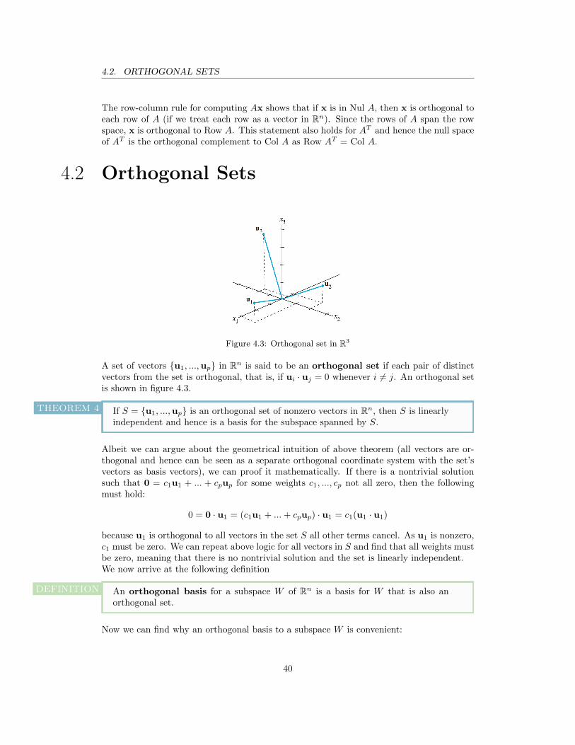
Figure 4.3: Orthogonal set in R3
A set of vectors {u1, ...,up} in Rn is said to be an orthogonal set if each pair of distinctvectors from the set is orthogonal, that is, if ui · uj = 0 whenever i 6= j. An orthogonal setis shown in figure 4.3.
If S = {u1, ...,up} is an orthogonal set of nonzero vectors in Rn, then S is linearlyindependent and hence is a basis for the subspace spanned by S.
THEOREM 4
Albeit we can argue about the geometrical intuition of above theorem (all vectors are or-thogonal and hence can be seen as a separate orthogonal coordinate system with the set’svectors as basis vectors), we can proof it mathematically. If there is a nontrivial solutionsuch that 0 = c1u1 + ... + cpup for some weights c1, ..., cp not all zero, then the followingmust hold:
0 = 0 · u1 = (c1u1 + ...+ cpup) · u1 = c1(u1 · u1)
because u1 is orthogonal to all vectors in the set S all other terms cancel. As u1 is nonzero,c1 must be zero. We can repeat above logic for all vectors in S and find that all weights mustbe zero, meaning that there is no nontrivial solution and the set is linearly independent.We now arrive at the following definition
An orthogonal basis for a subspace W of Rn is a basis for W that is also anorthogonal set.
DEFINITION
Now we can find why an orthogonal basis to a subspace W is convenient:
40

4.2. ORTHOGONAL SETS
Let {u1, ...,up} be an orthogonal basis for a subspace W of Rn. For each y in W ,the weights in the linear combination
y = c1u1 + ...+ cpup
are given by
cj =y · ujuj · uj
(j = 1, ..., p)
THEOREM 5
PROOF As in the preceding proof of the linear independence of an orthogonal set, we findthat:
y · u = (c1u1 + ...+ cpup) · u1 = c1(u1 · u1)
Since u1 · u1 is nonzero, the equation can be solved for c1. Geometrically speaking, we arefinding that part of vector y that lies on the line L formed by cu1 and then dividing this partof y by the length of the vector u1 to find the scalar weight c. Note how this computation ismore convenient than solving a system of linear combinations as used in previous chaptersto find the weights of a given linear combination.
An Orthogonal Projection
Given a nonzero vector u in Rn, consider the problem of decomposing a vector y in Rn intothe sum of two vectors, one a multiple of u and the other orthogonal to u. We wish to write
y = y + z
Where y = αu for some scalar α and z is some vector orthogonal to u. See figure 4.4.Given any scalar α we know that z = y− αu to satisfy the above equation. Then y− y’ is
Figure 4.4: Orthogonal projection of vector y on line spanned by vector u
orthogonal to u if and only if
0 = (y− αu) · u = y · u− (αu) · u = y · u− α(u · u)
That is, the decomposition of y is satisfied with z orthogonal to u if and only if α = y·uu·u
and y = y·uu·uu. The vector y is called the orthogonal projection of y onto u and the
vector z is called the component of y orthogonal to u. The geometrical interpretationof finding the weights of a linear combination as explained in the previous section is onceagain applicable here.If c is any nonzero scalar and if u is replaced by cu in the definition of y then the orthogonalprojection y does not change. We can say that the projection is determined by subspace Lspanned by u. Sometimes y is denoted by projLy and is called the orthogonal projectionof y onto L.
41
4.3. ORTHOGONAL PROJECTIONS
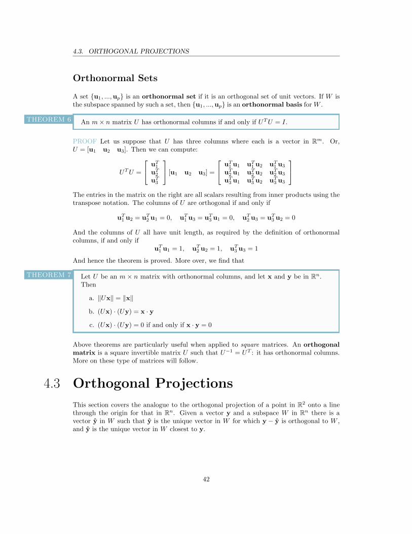
Orthonormal Sets
A set {u1, ...,up} is an orthonormal set if it is an orthogonal set of unit vectors. If W isthe subspace spanned by such a set, then {u1, ...,up} is an orthonormal basis for W .
An m× n matrix U has orthonormal columns if and only if UTU = I.THEOREM 6
PROOF Let us suppose that U has three columns where each is a vector in Rm. Or,U = [u1 u2 u3]. Then we can compute:
UTU =
uT1uT2uT3
[u1 u2 u3] =
uT1 u1 uT1 u2 uT1 u3
uT2 u1 uT2 u2 uT2 u3
uT3 u1 uT3 u2 uT3 u3
The entries in the matrix on the right are all scalars resulting from inner products using thetranspose notation. The columns of U are orthogonal if and only if
uT1 u2 = uT2 u1 = 0, uT1 u3 = uT3 u1 = 0, uT2 u3 = uT3 u2 = 0
And the columns of U all have unit length, as required by the definition of orthonormalcolumns, if and only if
uT1 u1 = 1, uT2 u2 = 1, uT3 u3 = 1
And hence the theorem is proved. More over, we find that
Let U be an m × n matrix with orthonormal columns, and let x and y be in Rn.Then
a. ‖Ux‖ = ‖x‖
b. (Ux) · (Uy) = x · y
c. (Ux) · (Uy) = 0 if and only if x · y = 0
THEOREM 7
Above theorems are particularly useful when applied to square matrices. An orthogonalmatrix is a square invertible matrix U such that U−1 = UT : it has orthonormal columns.More on these type of matrices will follow.
4.3 Orthogonal Projections
This section covers the analogue to the orthogonal projection of a point in R2 onto a linethrough the origin for that in Rn. Given a vector y and a subspace W in Rn there is avector y in W such that y is the unique vector in W for which y − y is orthogonal to W ,and y is the unique vector in W closest to y.
42

4.3. ORTHOGONAL PROJECTIONS
Figure 4.5: Geometric interpretation of orthogonal projection of y onto subspace W .
The Orthogonal Decomposition Theorem
Let W be a subspace of Rn. Then each y in Rn can be written uniquely in theform
y = y + z
where y is in W and z is in W⊥. In fact, if {u1, ...,up} is any orthogonal basis ofW , then
y =y · u1
u1 · u1u1 + ...+
y · upup · up
up
and z = y− y.
THEOREM 8
The vector y in above theorem is called the orthogonal projection of y onto W and isoften written as projWy.
Properties of Orthogonal Projections
The Best Approximation Theorem
Let W be a subspace of Rn, let y be any vector in Rn, and let y be the orthogonalprojection of y onto W . Then y is the closest point in W to y, in the sense that
‖y− y‖ < ‖y− v‖
for all v in W distinct from y.
THEOREM 9
The vector y in above theorem is called the best approximation to y by elements of W .
If the basis to subspace W is an orthonormal set:
If {u1, ...,up} is an orthonormal basis for a subspace W of Rn then
projWy = (y · u1)u1 + (y · u2)u2 + ...+ (y · up)up
if U = [u1 u2 ... up], then
projWy = UUTy for all y in Rn
THEOREM 10
43

4.4. THE GRAM-SCHMIDT PROCESS
PROOF The first equation follows directly from the orthogonal decomposition theorem asuj · uj = 1 for any vector uj in an orthonormal set. The second equation is another way ofwriting the first. Note how the first equation indicates that projWy is essentially a linearcombination of the vectors in the orthonormal basis with weights y ·uj . The equation UTyresults in a vector containing the result of all inner products of y with the rows of UT , andhence the columns of U . Thus, if this resulting vector is used to form a linear combinationwith the columns of U , we arrive back at the first equation.
4.4 The Gram-Schmidt Process
The Gram-Schmidt Process
Given a basis {x1, ...,xp} for a nonzero subspace W of Rn, define
v1 = x1
v2 = x2 −x2 · v1
v1 · v1v1
v2 = x3 −x2 · v1
v1 · v1v1 −
x3 · v2
v2 · v2v2
...
vp = xp −xp · v1
v1 · v1v1 −
xp · v2
v2 · v2v2 − ...−
xp · vp−1vp−1 · vp−1
vp−1
Then {v1, ...,vp} is an orthogonal basis for W . In addition
Span{v1, ...,vk} = Span{x1, ...,xk} for 1 ≤ k ≤ p
THEOREM 11
Suppose for some k < p we have constructed v1, ...,vk so that {v1, ...,vk} is an orthogonalbasis for Wk (note that this always possible as we start out with v1 = x1). If we define thenext vector to be added to the orthogonal set as:
vk+1 = xk+1 − projWkxk+1
By the orthogonal decomposition theorem we konw that vk+1 is orthogonal to Wk. We alsoknow that projWk
xk+1 is in Wk and is thus also in Wk. Now we know that vk+1 is in Wk+1
as the addition of two vectors in a given subspace always leads to another vector in thatsubspace (i.e. closed by addition and subtraction). We have now proven that v1, ...,vk+1 isan orthogonal set of nonzero vectors (making them all linearly independent) in the (k+ 1)-dimensional subspace Wk+1. By the basis theorem it follows that this set is a basis, andthus an orthogonal basis to Wk+1.
Note how we can use the Gram-Schmidt process to find an orthonormal basis by normalizingthe orthogonal basis resulting from the algorithm.
44
4.5. LEAST-SQUARES PROBLEMS
4.5 Least-Squares Problems
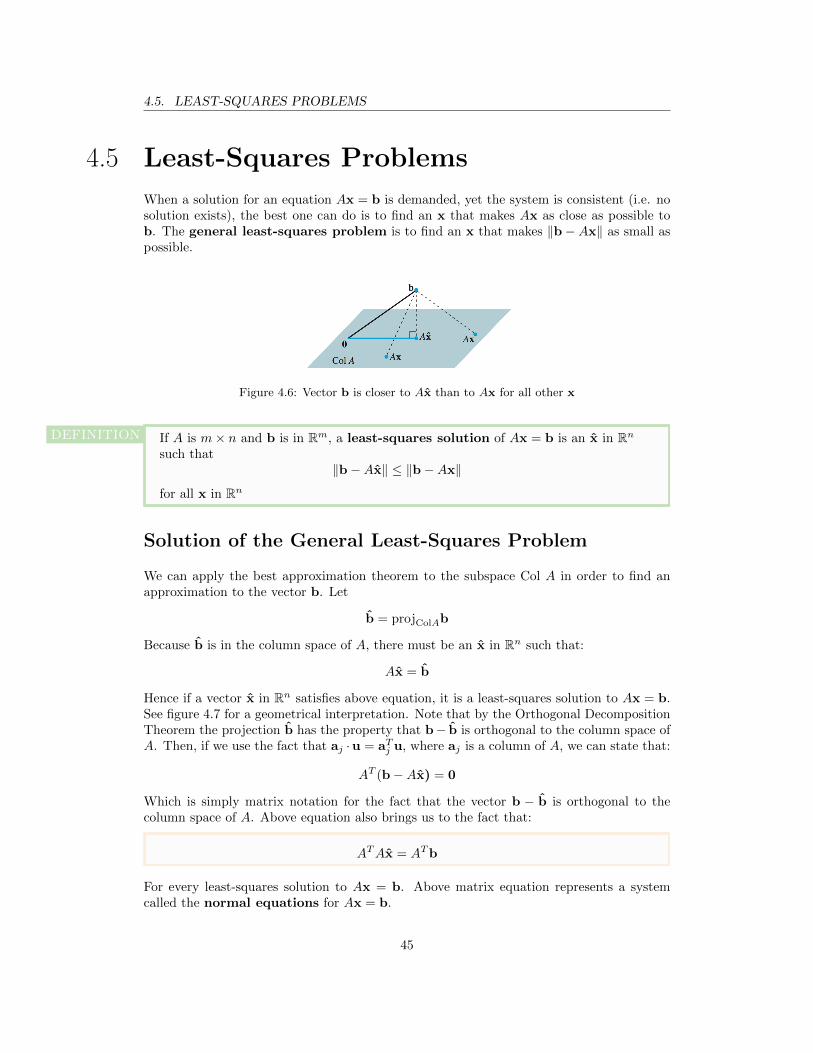
When a solution for an equation Ax = b is demanded, yet the system is consistent (i.e. nosolution exists), the best one can do is to find an x that makes Ax as close as possible tob. The general least-squares problem is to find an x that makes ‖b−Ax‖ as small aspossible.
Figure 4.6: Vector b is closer to Ax than to Ax for all other x
If A is m× n and b is in Rm, a least-squares solution of Ax = b is an x in Rnsuch that
‖b−Ax‖ ≤ ‖b−Ax‖
for all x in Rn
DEFINITION
Solution of the General Least-Squares Problem
We can apply the best approximation theorem to the subspace Col A in order to find anapproximation to the vector b. Let
b = projColAb
Because b is in the column space of A, there must be an x in Rn such that:
Ax = b
Hence if a vector x in Rn satisfies above equation, it is a least-squares solution to Ax = b.See figure 4.7 for a geometrical interpretation. Note that by the Orthogonal DecompositionTheorem the projection b has the property that b− b is orthogonal to the column space ofA. Then, if we use the fact that aj ·u = aTj u, where aj is a column of A, we can state that:
AT (b−Ax) = 0
Which is simply matrix notation for the fact that the vector b − b is orthogonal to thecolumn space of A. Above equation also brings us to the fact that:
ATAx = ATb
For every least-squares solution to Ax = b. Above matrix equation represents a systemcalled the normal equations for Ax = b.
45

4.6. APPLICATIONS TO LINEAR MODELS
Figure 4.7: A least squares solution
The set of least-squares solutions of Ax = b coincides with the nonempty set ofsolutions of the normal equations ATAx = ATb.
THEOREM 13
Solving the augmented matrix of the normal equations leads to a general expression of theset of least-squares solutions.
The next theorem gives useful criteria for determining when there is only one or more least-squares solution of Ax = b (note that the projection of b on Col A is always unique).
Let A be an m× n matrix. The following statements are logically equivalent:
a. The equation Ax = b has a unique least-squares solution for each b in Rm.
b. The columns of A are linearly independent.
c. The matrix ATA is invertible.
When these statements are true, the unique least-squares solution x is given by
x = (ATA)−1ATb
THEOREM 14
PROOF If statement (b) is true, we know that there are no free variables in any equationAx = v and there is one unique solution for every v in Col A, hence also for the least-squaressolution of Ax = b and thus statement (a) is true. Statement (c) follows from the fact thatthere is an unique solution x = (ATA)−1ATb.If a least-squares solution x is used to produce an approximation Ax to b, the distancebetween Ax and b is called the least-squares error of this approximation.
4.6 Applications to Linear Models
In this section, we denote the matrix equation Ax = b as Xβ = y and refer to X as thedesign matrix, β as the parameter vector, and y as the observation vector.
46
4.6. APPLICATIONS TO LINEAR MODELS
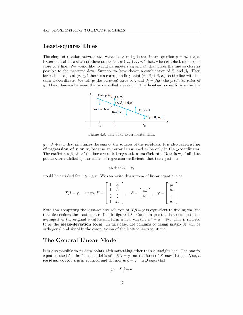
Least-squares Lines
The simplest relation between two variables x and y is the linear equation y = β0 + β1x.Experimental data often produce points (x1, y1), ..., (xn, yn) that, when graphed, seem to lieclose to a line. We would like to find parameters β0 and β1 that make the line as close aspossible to the measured data. Suppose we have chosen a combination of β0 and β1. Thenfor each data point (xi, yi) there is a corresponding point (xi, β0 +β1xi) on the line with thesame x-coordinate. We call yi the observed value of y and β0 + β1xi the predicted value ofy. The difference between the two is called a residual. The least-squares line is the line
Figure 4.8: Line fit to experimental data.
y = β0 + β1x that minimizes the sum of the squares of the residuals. It is also called a lineof regression of y on x, because any error is assumed to be only in the y-coordinates.The coeficients β0, β1 of the line are called regression coefficients. Note how, if all datapoints were satisfied by our choice of regression coefficients that the equation:
β0 + β1xi = yj
would be satisfied for 1 ≤ i ≤ n. We can write this system of linear equations as:
Xβ = y, where X =
1 x11 x2...
...1 xn
, β =
[β0β1
], y =
y1y2...yn
Note how computing the least-squares solution of Xβ = y is equivalent to finding the linethat determines the least-squares line in figure 4.8. Common practice is to compute theaverage x of the original x-values and form a new variable x∗ = x − x∗. This is referredto as the mean-deviation form. In this case, the columns of design matrix X will beorthogonal and simplify the computation of the least-squares solutions.
The General Linear Model
It is also possible to fit data points with something other than a straight line. The matrixequation used for the linear model is still Xβ = y but the form of X may change. Also, aresidual vector ε is introduced and defined as ε = y−Xβ such that
y = Xβ + ε
47

4.6. APPLICATIONS TO LINEAR MODELS
A data fit by curves has the general form
y = β0f0(x) + β1f1(x) + ...+ βnfn(x)
Which can be extended to the familiar matrix equation Xβ = y. Note that fi(x) may beany function of x, and is still used in a linear model as the coefficients βi are unknown.
48

5Eigenvalues and Eigenvectors
5.1 Eigenvectors and Eigenvalues
Figure 5.1: Note how u is an eigenvector of A as Au = −4u. Vector v is not an eigenvector
An eigenvector of an n× n matrix A is the nonzero vector x such that Ax = λxfor some scalar λ. A scalar λ is called an eigenvalue of A if there is a nontrivialsolution x of Ax = λx; such an x is called an eigenvector corresponding to λ.
DEFINITION
Note that we can also say that an eigenvector must satisfy:
Ax− λx = 0
For x 6= 0. Hence:(A− λI)x = 0
Must be satisfied. Thus the set of all eigenvectors for a given λ and matrix A is the nullspace of A− λI. This subspace of Rn is denoted as the eigenspace.
The eigenvalues of a triangular matrix are the entries on its main diagonal.THEOREM 1
PROOF Consider the case of a 3× 3 matrix A. If A is upper triangular, then:
A− λI =
a11 a12 a130 a22 a230 0 a33
− λ 0 0
0 λ 00 0 λ
=
a11 − λ a12 a130 a22 − λ a230 0 a33 − λ
49

5.2. THE CHARACTERISTIC EQUATION
Note that if A would have eigenvalues, then A − λI must have one or more free variablesas otherwise the equation would only be satisfied for the zero vector. Hence, one of thediagonal entries of A − λI must be zero (i.e. the matrix does not have a pivot positionin every column). Thus, for each diagonal entry of A, there exists an eigenvalue λ andaccompanying eigenvectors.
If v1, ...,vr are eigenvectors that correspond to distinct eigenvalues λ1, ..., λr of ann× n matrix A, then the set {v1, ...,vr} is linearly independent.
THEOREM 2
Eigenvectors and Difference Equations
A first-order difference equation is of the form:
xk+1 = Axk (k = 0, 1, 2, ...)
If A is n× n, then this a recursive (i.e. depending on the preceding term) description of asequence {xk} in Rn. We define a solution to be an explicit description of {xk} which doesnot depend directly on A or the preceding terms in the sequence other than the originalterm x0. The simplest way to such a solution is
xk = λkx0
Where x0 is an eigenvector and λ is its corresponding eigenvalue. Note that this holds since
Axk = A(λkx0) = λk(Ax0) = λk(λx0) = λk+1x0 = xk+1
This way of forming a solution makes sense, as we find an eigenvector with respectiveeigenvalue λ such that Ax0 = λx0 which is also in the respective eigenspace as it is simplya multiple of x0 ! Hence we can once again use scalar multiplication by λ to represent Ax,which may continue infinitely.
5.2 The Characteristic Equation
We start this section with an extension of the Invertible Matrix Theorem. The use of thisextension will become evident soon after.
The Invertible Matrix Theorem (continued)
Let A be an n× n matrix. Then A is invertible if and only if:
a. The number 0 is not an eigenvalue of A.
b. The determinant of A is not zero.
THEOREM
The Characteristic Equation
The following scalar equation allows one to directly find the eigenvalues of a square matrixA.
50

5.3. DIAGONALIZATION
A scalar λ is an eigenvalue of an n × n matrix A if and only if λ satisfies thecharacteristic equation
det(A− λI) = 0
This makes sense, since a determinant equal to zero indicates that the matrix is not invert-ible which indicates that it does contain free variables, which means that there are nontrivialsolutions to (A− λI)x = 0) and hence means that λ is an eigenvalue of A.
The n-degree polynomial in λ resulting from the computation of the determinant of an n×nmatrix is called the characteristic polynomial of A. The eigenvalues of A are the rootsof this polynomial. The multiplicity of an eigenvalue λ is its multiplicity as a root of thecharacteristic equation (i.e. how many times the scalar occurs as root).
Similarity
If A and B are n × n matrices, then A is similar to B if there is an invertible matrix Psuch that P−1AP = B, or, equivalently, A = PBP−1. We can also write Q = P−1 andthus Q−1BQ = A. Then A and B are similar. If we change A into P−1AP it is called asimilarity transformation.
I
f n × n matrices A and B are similar, then they have the same characteristicpolynomial and hence the same eigenvalues (with the same multiplicities).
THEOREM 4
PROOF If B = P−1AP , then
B − λI = P−1AP − λP−1P = P−1(AP − λP ) = P−1(A− λI)P
Then using the multiplicative property of determinants:
det(B − λI) = det[P−1(A− λI)P ] = det(P−1) · det(A− λI) · det(P )
Since det(P−1) · det(P ) = det(P−1P ) = det(I) = 1, we see that det(B − λI) = det(A− λI)and hence they have the same characteristic polynomial.
5.3 Diagonalization
This section discusses the useful concept of a diagonal matrix. If we have such a diagonalmatrix D
D =
[d11 00 d22
]
with d11 and d22 nonzero, we have that:
Dk =
[dk11 00 dk22
]
51
5.3. DIAGONALIZATION
If we recall from section 5.2 that a matrix A similar to D can be written as A = PDP−1
with P invertible, then we can easily find an expression to the k-th power of A. We callsuch a matrix A that is similar to a diagonal matrix, diagonalizable.
The Diagonalization Theorem
An n × n matrix A is diagonalizable if and only if A has n linearly independenteigenvectors. In fact, A = PDP−1, with D a diagonal matrix, if and only if thecolumns of P are n linearly independent eigenvectors of A. In this case, the diagonalentries of D are eigenvalues of A that correspond, repsectively, to the eigenvectorsin P .
THEOREM 5
In other words, A is diagonaliziable if and only if there are enough eigenvectors to form abasis of Rn. We call such a basis an eigenvector basis of Rn.
PROOF If P is an n × n matrix with columns v1, ...,vn, and if D is any diagonal matrixwith diagonal entries λ1, ..., λn, then
AP = A[v1 v2 ... vn] = [Av1 Av2 ... Avn]
and
PD = P
λ1 0 ... 00 λ2 ... 0...
......
0 0 ... λn
= [λ1v1 λ2v2 ... λnvn]
Now suppose that A is indeed diagonalizable and A = PDP−1. Then right-multipliyingthis equality with matrix P gives that AP = PD, implying that:
[Av1 Av2 ... Avn] = [λ1v1 λ2v2 ... λnvn]
If we equate columns we find that:Avj = λjvj
for 1 ≤ j ≤ n. As P is invertible, all columns are linearly independent and thus are nonzero.Hence, the equation above implies that λ1, λ2, ..., λn are indeed eigenvalues with correspond-ing eigenvectors v1,v2, ...,vn, which proves the theorem above.
The following theorem is a more brief condition than the previous theorem to see if a matrixis indeed diagonalizable.
An n× n matrix with n distinct eigenvalues is diagonalizable.THEOREM 6
PROOF Let λ1, ..., λn be distinct eigenvalues of a n × n matrix A, then v1, ...,vn are thecorresponding eigenvectors. By theorem 2 in section 5.1, these eigenvectors are linearlyindependent, hence there exists an invertible matrix P composed of n eigenvectors thussatisfying the requirement for A to be diagonalizable.
52
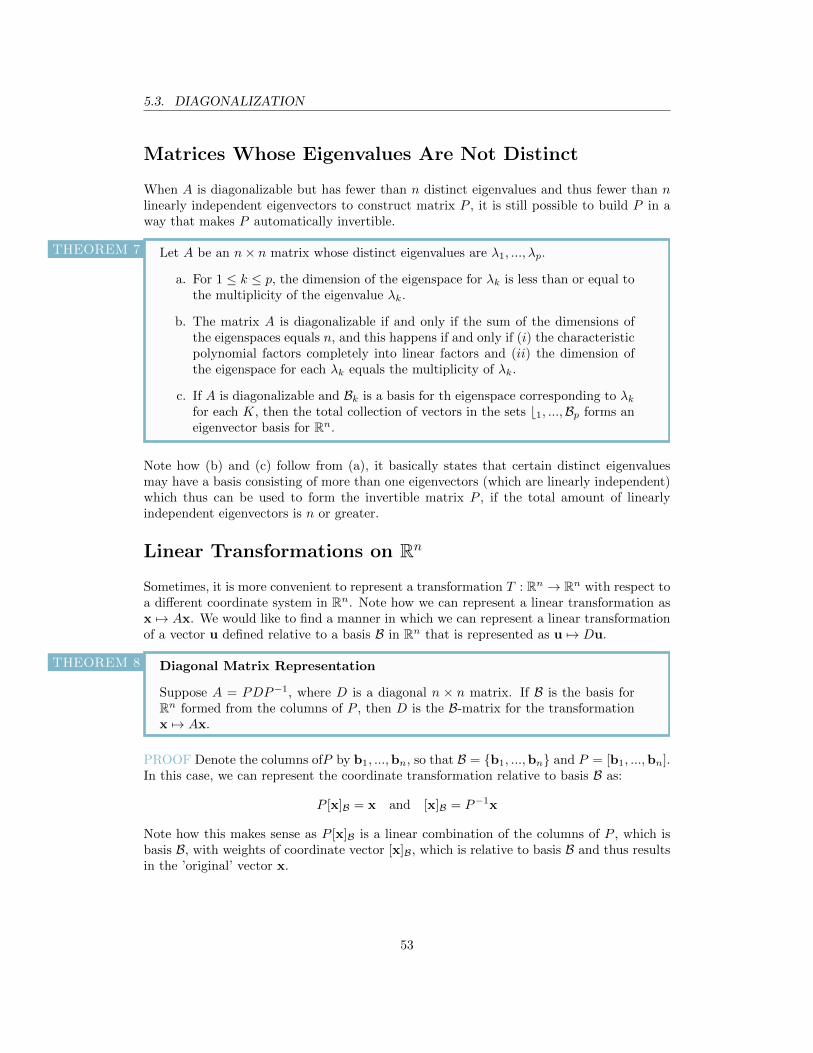
5.3. DIAGONALIZATION
Matrices Whose Eigenvalues Are Not Distinct
When A is diagonalizable but has fewer than n distinct eigenvalues and thus fewer than nlinearly independent eigenvectors to construct matrix P , it is still possible to build P in away that makes P automatically invertible.
Let A be an n× n matrix whose distinct eigenvalues are λ1, ..., λp.
a. For 1 ≤ k ≤ p, the dimension of the eigenspace for λk is less than or equal tothe multiplicity of the eigenvalue λk.
b. The matrix A is diagonalizable if and only if the sum of the dimensions ofthe eigenspaces equals n, and this happens if and only if (i) the characteristicpolynomial factors completely into linear factors and (ii) the dimension ofthe eigenspace for each λk equals the multiplicity of λk.
c. If A is diagonalizable and Bk is a basis for th eigenspace corresponding to λkfor each K, then the total collection of vectors in the sets b1, ...,Bp forms aneigenvector basis for Rn.
THEOREM 7
Note how (b) and (c) follow from (a), it basically states that certain distinct eigenvaluesmay have a basis consisting of more than one eigenvectors (which are linearly independent)which thus can be used to form the invertible matrix P , if the total amount of linearlyindependent eigenvectors is n or greater.
Linear Transformations on Rn
Sometimes, it is more convenient to represent a transformation T : Rn → Rn with respect toa different coordinate system in Rn. Note how we can represent a linear transformation asx 7→ Ax. We would like to find a manner in which we can represent a linear transformationof a vector u defined relative to a basis B in Rn that is represented as u 7→ Du.
Diagonal Matrix Representation
Suppose A = PDP−1, where D is a diagonal n × n matrix. If B is the basis forRn formed from the columns of P , then D is the B-matrix for the transformationx 7→ Ax.
THEOREM 8
PROOF Denote the columns ofP by b1, ...,bn, so that B = {b1, ...,bn} and P = [b1, ...,bn].In this case, we can represent the coordinate transformation relative to basis B as:
P [x]B = x and [x]B = P−1x
Note how this makes sense as P [x]B is a linear combination of the columns of P , which isbasis B, with weights of coordinate vector [x]B, which is relative to basis B and thus resultsin the ’original’ vector x.
53

5.4. COMPLEX EIGENVALUES
If T (x) = Ax for x in Rn, then
[T ]B = [[T (b1)]B ... ...[T (bn)]B]]
= [[Ab1]B, ... [Abn]B]
= [P−1Ab1 ... P−1Abn]
= P−1A[b1 ... bn]
= P−1AP
Since A = PDP−1, we have [T ]B = P−1AP = D, which proves above theorem.
5.4 Complex Eigenvalues
Since the characteristic equation of an n× n matrix involves a polynomial of degree n, theequation always has exactly n roots, counting multiplicities, provided that possibly complexroots are included. The key is to let A also act on the space Cn of n-tuples of complexnumbers.
The matrix eigenvalue-eigenvector theory already developed for Rn applies equally well toCn. So a complex scalar λ if and only if there is a nonzero vector x in Cn such that Ax = x.
Real and Imaginary parts of Vectors
The complex conjugate of a complex vector x in Cn is the vector x in Cn whose entries arethe complex conjugates of the entries in x. The real and imaginary parts of a complexvector x are the vectors Re x and Im x in Rn formed from the real and imaginary parts ofthe entries of x
For example, if x =
3− ii
2 + 5i
=
302
+ i
−115
, then
Re x =
302
, Im x =
−115
, and x =
302
− i −1
15
=
3 + i−i
2− 5i
If B is an m × n matrix with possibly complex entries, then B denotes the matrix whoseentries are the complex conjugates of the entries in B. Properties of conjugates for complexnumbers carry over to complex matrix algebra:
rx = rx, Bx = Bx, BC = BC, and rB = rB
54

5.5. APPLICATIONS TO DIFFERENTIAL EQUATIONS
Eigenvalues and Eigenvectors of a Real matrix That Actson Cn
Let A be an n×n matrix whose entries are real. Then Ax = Ax = Ax. If λ is an eigenvalueof A and x is a corresponding eigenvector in Cn, then
Ax = Ax = λx = λx
Hence λ is also an eigenvalue of A, with x a corresponding eigenvector. This shows thatwhen A is real, its complex eigenvalues occur in conjugate pairs. A complex eigenvaluerefers to an eigenvalue of the form λ = a+ bi, with b 6= 0.
If C =
[a −bb a
]where a and b are real and not both zero, then the eigenvalues of C are
5.5 Applications to Differential Equations
In many applied problems, several quantities are varying continuously in time, and they arerelated by a system of differential equations:
x′1 = a11x1 + ...+ a1nxn
...
x′n = an1x1 + ...+ annxn
Where x1, ..., xn are differentiable functions of t, with derivatives x′1, ..., x′n and constants
aij . The crucial feature of the system above is that it is indeed linear. In order to see thiswe write the system in matrix notation and find:
x′(t) = Ax(t)
where
x(t) =
x1(t)...
xn(t)
, x′(t) =
x′1(t)...
x′n(t)
, and A =
a11 ... a1n...
...an1 ... ann
A solution of equation 5.5 is a vector-valued function that satisfies the equation for all t insome intervfal of real numbers, such as t ≥ 0. Th equation is linear because both differenti-ation of a function and multiplication of vectors by a matrix are linear transformations. Ifu and v are both solutions of x′ = Ax, then cu + dv is also a solution because
(cu + dv)′ = cu′ + cv′
= cAu + dAv = A(cu + dv)
55

5.5. APPLICATIONS TO DIFFERENTIAL EQUATIONS
Note that the zero function is a trivial solution of x′ = Ax. It can be shown that therealways exists what is called a fundamental set of solutions to 5.5. If A is n × n, thenthere are n linearly independent functions in a fundamental set, and each solution of 5.5 isa unique linear combination of these n functions. If a vector x0 is specified, then the initialvalue problem is to construct the function x such that x′ = Ax and x(0) = x0. When Ais diagonal, the solution of such a system of differential equations is simple, consider:[
x′1(t)x′2(t)
]=
[3 00 −5
] [x1(t)x2(t)
]Which represents the system
x′1(t) = 3x1(t)
x′2(t) = −5x2(t)
The system is said to be decoupled as each derivative only depends on its own initial function.The solution to the system is[
x1(t)x2(t)
]=
[c1e
3t
c2e−5t
]= c1
[10
]e3t + c2
[01
]e−5t
Which suggests that for the general equation x′ = Ax, a solution might be a linear combi-nation of functions of the form
x(t) = veλt
for some scalar λ and some fixed nonzero vector v. Observe that, by this suggested solutionwe have that
x′(t) = λveλt
Ax(t) = Aveλt
As eλt is never zero, x′(t) will equal Ax(t) if and only if λv = Av, that is, if and only if λ isan eigenvalue of A and v is a corresponding eigenvector. Thus each eigenvalue-eigenvectorpair provides a solution of x′ = Ax.
Figure 5.2: Origin functioning as a saddle point on the left and as an attractor on the right
Note that if we have two solutions to a system x′(t) = Ax(t), namely x1 and x2, that anylinear combination of these is also a solution of the system by the linearity of differentiationand matrix transformation. Note that the behavior of the solution depends on the exponentλ. If all exponents are negative, the origin functions as an attractor as for large values oft the solution x(t) will approach zero, which is opposite to the behavior of a solution withonly positive exponents. If one exponent is negative and the other is positive, the originfunctions as a saddle point. Both are shown in figure 5.2.
56

5.5. APPLICATIONS TO DIFFERENTIAL EQUATIONS
Decoupling a Dynamical System
The following discussion shows that the method treated in the previous section producesa fundamental set of solutions for any dynamical system described by x′ = Ax when A isn × n and has n linearly independent eigenvectors (i.e. A is diagonalizable). Suppose theeigenfunctions for A are
v1eλ1t, ...,vne
λnt
With v1, ...,vn linearly independent eigenvectors. Let P = [v1...vn] and let D be thediagonal matrix with entries λ1, ..., λn so that A = PDP−1. Now make a change of variable,defining a new function y by
y(t) = P−1x(t) or, equivalently, x(t) = Py(t)
Note how y(t) is the coordinate vector of x(t) relative to the eigenvector basis. If wesubstitute Py in x′ = Ax
d
dt(Py) = A(Py) = (PDP−1)Py = PDy
Since P is a constant matrix, the left side is differentiated to Py′, hence if we left multiplyboth equations with P−1 we have that y′ = Dy, or
y′1(t)y′2(t)
...y′n(t)
=
λ1 0 ... 0
0 λ2...
.... . . 0
0 ... 0 λn
y1(t)y2(t)
...yn(t)
By change of variable from x to y we have decoupled the system of differential equations.Now the solution is simply:
y(t) =
c1eλ1t
...cne
λnt
, where
c1...cn
= y0 = P−1x0
To obtain the general solution x of the original system
x(t) = Py(t) = [v1 ... vn]y(t)
= c1v1eλ1t + ...+ cnvne
λnt
Complex Eigenvalues
First recall that the complex eigenvalues of a real matrix always come in conjugate pairs.Then, we have that two solutions of x′ = Ax are
x1(t) = veλt and x2(t) = veλt
Note that above eigenfunctions are complex, and that most applications require real eigen-functions. Fortunately, the real and imaginary parts of x1 are real solutions of x′ = Ax,because they are linear combinations of the solutions above:
Re(veλt) =1
2[x1(t) + x1(t)], Im(veλt) =
1
2i[x1(t)− x1(t)]
57

5.5. APPLICATIONS TO DIFFERENTIAL EQUATIONS
So let us find an expression for the real and imaginary parts of x1. Recall that it is possible,by the use of Maclaurin series, to show that
eλt = e(a+bi)t = eat · eibt = eat(cos bt+ i sin bt)
By use of this fact the two real solutions of x′ = Ax are
y1(t) = Re x1(t) = [(Re v)cos bt− (Im v)sin bt]eat
y2(t) = Im x1(t) = [(Re v)sin bt+ (Im v)cos bt]eat
Moreover, it can be shown that y1(t) and y2(t) are linearly independent functions (whenb 6= 0).
58

6Symmetric Matrices and QuadraticForms
6.1 Diagonalization of Symmetric Matrices
A symmetric matrix is a matrix A such that AT = A, which means that A must be square.Note that its main diagonal entries may be arbitrary, whereas other entries occur in pairson opposite sides of the main diagonal.
A =
a b cb d ec e f
= AT
If A is symmetric, then any two eigenvectors from different eigenspaces are orthog-onal.
THEOREM 1
Proof Let v1 and v2 be eigenvectors that correspond to distinct eigenvalues, say, λ1 and λ2.To show that v1 · v2 = 0, compute
λv1 · v2 = (λ1v1)Tv2 = (Av1)Tv2
= (vT1 AT )v2 = vT1 (Av2)
= vT1 (λ2v2)
= λ2vT1 v2 = λ2v1 · v2
Hence (λ1 − λ2)v1 · v2 = 0. But λ1 − λ2 6= 0, so v1 · v2 = 0.An n× n matrix A is said to be orthogonally diagonalizable if is an orthogonal matrixP (with P−1 = PT ) and a diagonal matrix D such that
A = PDPT = PDP−1
The diagonalization of above requires n linearly independent orthonormal eigenvectors.When is this possible? If A is orthogonally diagonalizable, then
AT = (PDPT )T = PTTDTPT = PDPT = A
Thus it is possible if A is symmetric. We can then reason the following:
An n × n matrix A is orthogonally diagonalizable if and only if A is a symmetricmatrix.
THEOREM 2
59

6.2. QUADRATIC FORMS
The Spectral Theorem
The set of eigenvalues of a matrix A is sometimes called the spectrum of A, and the followingdescription fo the eigenvalues is called a spectral theorem.
The Spectral Theorem for Symmetric Matrices
An n× n symmetric matrix A has the following properties:
a. A has n real eigenvalues, counting multiplicities.
b. The dimension of the eigenspace for each eigenvalue λ equals the multiplicityof λ as a root of the characteristic equation.
c. The eigenspaces are mutually orthogonal, in the sense that eigenvectors cor-responding to different eigenvalues are orthogonal.
d. A is orthogonally diagonalizable.
THEOREM 3
PROOF Property (a) can be proven by the fact that any vector x in Cn satisfies thatq = xTAx is real, hence λ must be real as xTAx = xλx and xTx is real. Part (c) isTheorem 1. Statement (b) follows from (d).
Spectral Decomposition
Suppose A = PDP−1, where the columns of P are orthonormal eigenvectors u1, ...,un ofA and the corresponding eigenvalues λ1, ..., λn are in the diagonal matrix D. Then, sinceP−1 = PT ,
A = PDPT = [u1 ... u2]
λ1 0. . .
0 λn
uT1
...uTn
= [λ1u1 ... nun]
uT1...
uT2
Then we can represent A as follows:
A = λ1u!uT1 + λ2u2u
T2 + ...+ λnunuTn
This representation of A is called a spectral decomposition of A because it breaks up Ainto terms determined by the spectrum (i.e. eigenvalues) of A. Note how every term is ann× n matrix of rank 1. Why? Each column of matrix λjuju
Tj is a multiple of uj .
6.2 Quadratic Forms
A quadratic form on Rn is a function Q defined on Rn whose value at a vector x in Rn canbe computed by an expression of the form Q(x) = xTAx, where A is an n × n symmetric
60

6.2. QUADRATIC FORMS
matrix. The matrix A is called the matrix of the quadratic form. Note how the simplestexample of a nonzero quadratic form is the inner product Q(x) = xT Ix = ‖x‖2.
Change of Variable in a Quadratic Form
If x represents a variable vector in Rn, then a change of variable is an equation of theform
x = Py, or equivalently, y = P−1x
where P is an invertible matrix and y is a new variable vector in Rn. Here y is the coordinatevector of x relative to the basis of Rn determined by the columns of P .If the change of variable is made in a quadratic form xTAx, then
Figure 6.1: Change of variable in xTAx
xTAx = (Py)TA(Py) = yTPTAPy = yT (PTAP )y
and the new matrix of the quadratic form is PTAP . Since A is symmetric, Theorem 2guarantees that there is an orthogonal matrix P such that PTAP is a diagonal matrix D,and we can write the quadratic form as yTDy. Why would we do this? By ensuring thatthe matrix of the quadratic form is diagonal, we avoid cross-product terms. Hence we havethe following theorem:
The Principal Axes Theorem
Let A be an n × n symmetric matrix. Then there is an orthogonal change ofvariable, x = Py that transforms the quadratic form xTAx into a quadratic formyTDy with no cross-product term.
THEOREM 4
The columns of P in the theorem are called the principal axes of the quadratic form xTAx.The vector y is the coordinate vector of x relative to the orthonormal basis of Rn given bythese principal axes.
A Geometric View of Principal Axes
Suppose Q(x) = xTAx, where A is an invertible 2 × 2 symmetric matrix, and let c be aconstant. It can be shown that the set of all x in R2 that satisfy
xTAx = c
61

6.2. QUADRATIC FORMS
either corresponds to an ellipse (or circle), a hyperbola, two intersecting lines, or a singlepoint, or contains no points at all. If A is a diagonal matrix, the graph is in standard positionas in figure 6.2. If A is not diagonal, the graph is rotated out of standard position as cross-
Figure 6.2: An ellipse and hyperbola in standard position
product terms are introduced. Finding the principal axes (determined by the eigenvectorsof A) amounts to finding a new coordinate system with respect to which the graph is instandard position, as shown in figure 6.3.
Figure 6.3: An ellipse and hyperbola not in standard position
Classifying Quadratic Forms
When A is an n × n matrix, the quadratic form Q(x) = xTAx is a real-valued functionwith domain Rn. Figure 6.4 shows four quadratic forms with domain R2, where the points(x1, x2, z) with z = Q(x) are plotted.
Figure 6.4: Graphs of quadratic forms. Classifications: (a) positive definite, (b) positive semidefi-nite, (c) indefinite, (d) negative definite
62

6.2. QUADRATIC FORMS
A quadratic form Q is:
a. positive definite if Q(x) > 0 for all x 6= 0,
b. negative definite if Q(x) < 0 for all x 6= 0,
c. indefinite if Q(x) assumes both positive and negative values.
DEFINITION
In addition to this definition, Q is said to be positive semidefinite if Q(x) ≥ 0 for all x,and to be negative semidefinite if Q(x) ≤ 0 for all x. Note how both (a) and (b) in figure6.4 are positive semidefinite, but the form in (a) is also positive definite.
Quadratic Forms and Eigenvalues
Let A be an n× n symmetric matrix. Then a quadratic form xTAx is:
a. positive definite if and only if the eigenvalues of A are all positive,
b. negative definite if and only if the eigenvalues of A are all negative, or
c. indefinite if and only if A has both positive and negative eigenvalues.
THEOREM 5
PROOF By the Principal Axes Theorem, there exists an orthogonal change of variablex = Py such that
Q(x) = xTAx = yTDy = λ1y21 + λ2y
22 + ...+ λny
2n
where λ1, ..., λn are the eigenvalues of A.
63