Linear Algebra Notes

Remkes KooistraThe King’s University

September 19, 2016

Contents

1 Introduction 1

1.1 What is Linear Algebra . . . . . . . . . . . . . . . . . . . . . . . . . . . . . . . . . . . . 1

1.2 Vectors and Matrices . . . . . . . . . . . . . . . . . . . . . . . . . . . . . . . . . . . . . . 1

2 Vector Geometry 5

2.1 Definitions . . . . . . . . . . . . . . . . . . . . . . . . . . . . . . . . . . . . . . . . . . . . 5

2.2 Linear Operations . . . . . . . . . . . . . . . . . . . . . . . . . . . . . . . . . . . . . . . 8

2.3 The Dot Product . . . . . . . . . . . . . . . . . . . . . . . . . . . . . . . . . . . . . . . . 11

2.4 The Cross Product . . . . . . . . . . . . . . . . . . . . . . . . . . . . . . . . . . . . . . . 14

2.5 Local Direction Vectors . . . . . . . . . . . . . . . . . . . . . . . . . . . . . . . . . . . . 15

2.6 Projections . . . . . . . . . . . . . . . . . . . . . . . . . . . . . . . . . . . . . . . . . . . 17

2.7 Objects in Rn . . . . . . . . . . . . . . . . . . . . . . . . . . . . . . . . . . . . . . . . . . 18

2.8 Linear and Affine Subspaces . . . . . . . . . . . . . . . . . . . . . . . . . . . . . . . . . . 21

2.9 Loci . . . . . . . . . . . . . . . . . . . . . . . . . . . . . . . . . . . . . . . . . . . . . . . 22

2.10 Spans . . . . . . . . . . . . . . . . . . . . . . . . . . . . . . . . . . . . . . . . . . . . . . 24

2.11 Dimension and Basis . . . . . . . . . . . . . . . . . . . . . . . . . . . . . . . . . . . . . . 25

2.12 Standard Forms . . . . . . . . . . . . . . . . . . . . . . . . . . . . . . . . . . . . . . . . . 26

1

3 Systems of Linear Equations 28

3.1 Definitions . . . . . . . . . . . . . . . . . . . . . . . . . . . . . . . . . . . . . . . . . . . . 28

3.2 Matrix Representation of Systems . . . . . . . . . . . . . . . . . . . . . . . . . . . . . . 29

3.3 Row Operations and Gaussian Elimination . . . . . . . . . . . . . . . . . . . . . . . . . 31

3.4 Solution Spaces and Free Parameters . . . . . . . . . . . . . . . . . . . . . . . . . . . . . 32

3.5 Dimensions of Spans . . . . . . . . . . . . . . . . . . . . . . . . . . . . . . . . . . . . . . 35

3.6 Dimensions of Loci . . . . . . . . . . . . . . . . . . . . . . . . . . . . . . . . . . . . . . . 36

4 Transformations of Euclidean Spaces 37

4.1 Definitions . . . . . . . . . . . . . . . . . . . . . . . . . . . . . . . . . . . . . . . . . . . . 37

4.2 Transformations of R2 or R3 . . . . . . . . . . . . . . . . . . . . . . . . . . . . . . . . . . 38

4.3 Symmetry and Dihedral Groups . . . . . . . . . . . . . . . . . . . . . . . . . . . . . . . . 40

4.4 Matrix Representation . . . . . . . . . . . . . . . . . . . . . . . . . . . . . . . . . . . . . 41

4.5 Matrices in R2 . . . . . . . . . . . . . . . . . . . . . . . . . . . . . . . . . . . . . . . . . 42

4.6 Composition and Matrix Multiplication . . . . . . . . . . . . . . . . . . . . . . . . . . . 44

4.7 Inverse Matrices . . . . . . . . . . . . . . . . . . . . . . . . . . . . . . . . . . . . . . . . 45

4.8 Transformations of Spans and Loci . . . . . . . . . . . . . . . . . . . . . . . . . . . . . . 46

4.9 Row and Columns Spaces, Kernels and Images . . . . . . . . . . . . . . . . . . . . . . . 47

4.10 Decomposition of Transformation . . . . . . . . . . . . . . . . . . . . . . . . . . . . . . . 49

5 Determinants 50

5.1 Definition . . . . . . . . . . . . . . . . . . . . . . . . . . . . . . . . . . . . . . . . . . . . 50

5.2 Calculation of Determinants . . . . . . . . . . . . . . . . . . . . . . . . . . . . . . . . . . 51

5.3 Triangular and Diagonal Determinants . . . . . . . . . . . . . . . . . . . . . . . . . . . . 54

5.4 Properties of Determinants . . . . . . . . . . . . . . . . . . . . . . . . . . . . . . . . . . 55

5.5 Traces . . . . . . . . . . . . . . . . . . . . . . . . . . . . . . . . . . . . . . . . . . . . . . 56

5.6 Cramer’s Rule . . . . . . . . . . . . . . . . . . . . . . . . . . . . . . . . . . . . . . . . . . 57

2

6 Orthogonality and Symmetry 58

6.1 Symmetry, Again . . . . . . . . . . . . . . . . . . . . . . . . . . . . . . . . . . . . . . . . 58

6.2 Matrices of Determinant One . . . . . . . . . . . . . . . . . . . . . . . . . . . . . . . . . 58

6.3 Orthogonal and Special Orthogonal Matrices . . . . . . . . . . . . . . . . . . . . . . . . 59

6.4 Orthogonal Bases and the Gram-Schmidt Process . . . . . . . . . . . . . . . . . . . . . . 60

6.5 Conjugation . . . . . . . . . . . . . . . . . . . . . . . . . . . . . . . . . . . . . . . . . . . 63

7 Eigenvectors and Eigenvalues 66

7.1 Definitions . . . . . . . . . . . . . . . . . . . . . . . . . . . . . . . . . . . . . . . . . . . . 66

7.2 Calculation of Eigenvalue and Eigenvectors . . . . . . . . . . . . . . . . . . . . . . . . . 67

7.3 Diagonalization . . . . . . . . . . . . . . . . . . . . . . . . . . . . . . . . . . . . . . . . . 70

8 Iterated Processes 73

8.1 General Theory . . . . . . . . . . . . . . . . . . . . . . . . . . . . . . . . . . . . . . . . . 73

8.2 Recurrence Relations . . . . . . . . . . . . . . . . . . . . . . . . . . . . . . . . . . . . . . 74

8.3 Linear Difference Equations . . . . . . . . . . . . . . . . . . . . . . . . . . . . . . . . . . 78

8.4 Markov Chains . . . . . . . . . . . . . . . . . . . . . . . . . . . . . . . . . . . . . . . . . 81

8.5 Gambler’s Ruin . . . . . . . . . . . . . . . . . . . . . . . . . . . . . . . . . . . . . . . . . 83

3

License

This work is licensed under the Creative Commons Attribution-ShareAlike 4.0 International License.

Chapter 1

Introduction

1.1 What is Linear Algebra

Algebra is the study of basic mathematical operations (such as addition and multiplication) and howthese operations interact with variables, functions and equations. Starting with the basic operations ofarithmetic on numbers (addition, multiplication, subtraction, division), algebra abstracts these familiarstructures and asks what similar structures exist for other sets. It finds new settings to expand theideas of addition and multiplication; in those new contexts, it wonders which properties still hold andwhich fail.

Linear algebra is the subset of algebra which deals with linear objects. The word ‘linear’ reminds ofus lines. This geometric intuition is correct: linear algebra deals with lines, but not only lines. Thestraightness of lines is the important property. Linear algebra is algebra dealing with straight or flatobjects.

Since we’re talking about lines and flat objects, we’re actually doing geometry. The lines, planes andother flat objects which we want to study are geometric objects. Therefore, linear algebra is a geometricdiscipline. It is the geometry of flat or straight objects. Many texts will start linear algebra with thealgebraic side of the discpline: using vectors and matrices to solve equations and systems of equations.These notes take the opposite approach and start with the geometric side of the discpline.

1.2 Vectors and Matrices

We start with the two most important definitions in linear algebra: the vector and the matrix.

1

Definition 1.2.1. In linear algebra, ordinary numbers (intergers, rational numbers or real numbers)are called scalars.

Definition 1.2.2. A vector is a finite ordered list of scalars. Vectors can be written either as columnsor rows. The scalars in a vector are called its entries, components or coordinates. If our vector hascomponents 4, 15, π and −e (in that order), we write the vector in one of two ways.

415πe

or (4, 15, π,−e)

In these notes, we will exclusively use column vectors.

Definition 1.2.3. A matrix is a rectangular array of scalars. If the matrix has m rows and n columns,we say it is an m×n matrix. The scalars in the matrix are called the entries, components or coefficients.

A matrix is written as a rectangular array of numbers, either in square or round brackets. Here aretwo ways of writing a particular 3× 2 matrix with integer coefficients.

5 6−4 −40 −3

5 6−4 −40 −3

The rows of this matrix are these three vectors:(

56

) (−4−4

) (0−3

)

The columns of this matrix are these two vectors:

5−40

6−4−3

In these notes, we’ll use curved brackets for matrices; however, in many texts and books, square bracketsare very common. Both notations are conventional and acceptable.

If we want to write a general matrix, we can write it this way:

a11 a12 . . . a1na21 a22 . . . a2n. . . . . . . . . . . .an1 an2 . . . ann

2

By convention, when we write an aribitrary matrix entry aij the first index tells us the row and thesecond index tells us the column. For example, a64 is the entry in the sixth row and the fourth column.In the rare occurence that we have matrices with more than 10 rows or columns, we can seperate theindices by commas: a12,15 would be in the twelfth row and the fifteenth column. Row and columnindexing is very convenient. Sometime we even write A = aij as short-hand for a matrix when the sizeis understood.

Here are some initial definitions:

Definition 1.2.4. The rows of a matrix are called the row vectors of the matrix. Likewise the columnsare called column vectors of the matrix.

Definition 1.2.5. A square matrix is a matrix with the same number of rows as columns.

4 −2 8−3 −3 −30 0 −1

0 0 0 1 01 0 0 1 01 0 1 1 00 1 0 0 00 1 1 1 0

Definition 1.2.6. The zero matrix is the unique matrix (one for every size m × n) where all thecoefficients are all zero.

0 00 00 0

0 0 0 0 0 00 0 0 0 0 00 0 0 0 0 00 0 0 0 0 00 0 0 0 0 00 0 0 0 0 0

Definition 1.2.7. The diagonal entries of a matrix are all entries aii where the row and columnindices are the same. A diagonal matrix is a matrix where all the non-diagonal entries are zero.

5 00 20 0

1 0 0 00 −4 0 00 0 8 00 0 0 0

Definition 1.2.8. The identity matrix is the unique n×n matrix (one for each n) where the diagonalentries are all 1 and all other entries are 0.

(1 00 1

)

1 0 00 1 00 0 1

1 0 0 00 1 0 00 0 1 00 0 0 1

Definition 1.2.9. An upper triangular matrix is a matrix where all entries below the diagonal arezero. A lower triangular matrix is a matrix where all entries above the diagonal are zero.

−1 3 50 2 −90 0 1

0 0 2 20 −7 4 00 0 9 −40 0 0 −4

3

Definition 1.2.10. The transpose of a matrix is the matrix formed by switching the rows and columns.Alternatively, it is the mirror of the matrix over the diagonal. If A = aij is a matrix expressed in indices,then the transpose is written AT and has entries aji with indices switched.

A =

3 0 6 −14 −2 −7 06 −6 −1 −2

AT =

3 4 60 −2 −66 −7 −1−1 0 −2

A =

0 0 8 −50 1 1 −20 6 6 −10 0 −4 −4

AT =

0 0 0 00 1 6 08 1 6 −4−5 −2 −1 −4

Definition 1.2.11. A n× n matrix A is symmetric if A = AT .

5 1 −31 2 0−3 0 4

1 4 −2 −94 −4 3 3−2 3 8 −1−9 3 −1 7

Column vectors are just m × 1 matrices and row vectors are just 1 ×m matrices. Sometimes, whenmathematicians want to keep track of the fact that they treat a vector as a column, they will use thetranspose operator:

−2−206

= (−2,−2, 0, 6)T

Sometimes it is useful add seperation to the organization of the matrix.

Definition 1.2.12. An extended matrix is a matrix with a vertical division seperating the columnsinto two groups.

−3 0 6 14 −2 2 −10 0 3 −7

It is convenient to fix notation for collections of matrices of certain sizes.

Definition 1.2.13. The set of all n×m matrices with real coefficients is written Mn,m(R). For squarematrices (n× n), we simply write Mn(R).

4

Chapter 2

Vector Geometry

Vector geometry is the study of positions and directions in straight-line geometry. We first need toestablish the basic environment.

2.1 Definitions

Definition 2.1.1. Let n be a positive integer. Real Euclidean Space or Cartesian Space, written Rn,is the set of all vectors with real number entries. An arbitrary element of Rn is written as a column.

x1x2...xn

We say that Rn has dimension n.

Definition 2.1.2. The scalars xi in a vector are called the entries, coordinates or components of thatvector. Specifically, x1 is the first coordinate, x2 is the second coordinate, and so on. For R2, R3 andR4, we use the letters x, y, z, w instead of xi.

(xy

)∈ R2

xyz

∈ R3

wxyz

∈ R4

5

y

x

(36

)

(00

)

(4−4

)

(−5−2

)

(−77

)

Figure 2.1: Points in the Carteian Plane R2

Definition 2.1.3. In any Rn, the origin is the unique point given by a vector of zeros. It is also calledthe zero vector.

00...0

It is considered the centre point of Cartesian space.

Cartesian space, particularly the Cartesian plane, is a familiar object from high-school mathematics.We usually visualize Cartesian space by way of drawing axes: one in each independent perpendicular

direction. In this visualization, the vector(ab

)corresponds to the unique point we get moving a units

in the direction of the x axis and b units in the direction of the y axis.

As with R2, the point

abc

∈ R3 is the unique point we find by moving a units in the x direction, b units

in the y direction and c units in the z direction.

6

Figure 2.2: Points in Cartesian three-space R3

When we visualize R2, we conventionally write the x axis horizontally, with a positive direction to theright, and the y axis vertically, with a positive direction upwards. There are similar conventions forR3.

Definition 2.1.4. A choice of axis directions in a visualization of Rn is called an orientation.

While we can visualize R2 and R3 relatively easily and efficiently, but we can’t visualize any higher Rn.However, that doesn’t prevent us from working in higher dimensions. We need to rely on the algebraicdescriptions of vectors instead of the drawings and visualizations of R2 and R3.

In our visualizations of R2 and R3, we see the different axes as fundementally different perpendiculardirections. We can think of R2 as the space with two independent directions and R3 as the space withthree independent directions. Similarly, R4 is the space with four perpendicular, independent directions,even though it is impossible to visualize such a thing. Likewise, Rn is the space with n independentdirections.

2.1.1 Vectors as Points and Directions

We can think of a element of R2, say(

14

), as both the point located at

(14

)and the vector drawn from

the origin to the point(

14

). Though these two ideas are distinct, we will frequently change perspective

7

y

x

Point:

(14

)

Vector:

(14

)

Point:

(42

)

Vector:

(42

)

Figure 2.3: Vectors as Points and Directions

between them. Part of becoming proficient in vector geometry is becoming accustomed to the switchbetween the perspectives of points and directions.

2.2 Linear Operations

The previous section built the environment for linear algebra: Rn. Algebra is concerned with operationson sets, so we want to know what operations we can perform on Rn. There are several.

Definition 2.2.1. The sum of two vectors u and v in Rn is the sum taken componentwise.

u+ v =

u1u2...un

+

v1v2...vn

=

u1 + v1u2 + v2

...un + vn

Note that we can only add two vectors in the same dimension. We can’t add a vector in R2 to a vectorin R3.

8

y

x

u =

(13

)

v =

(31

)

u =

(13

)

v =

(31

)

u+ v

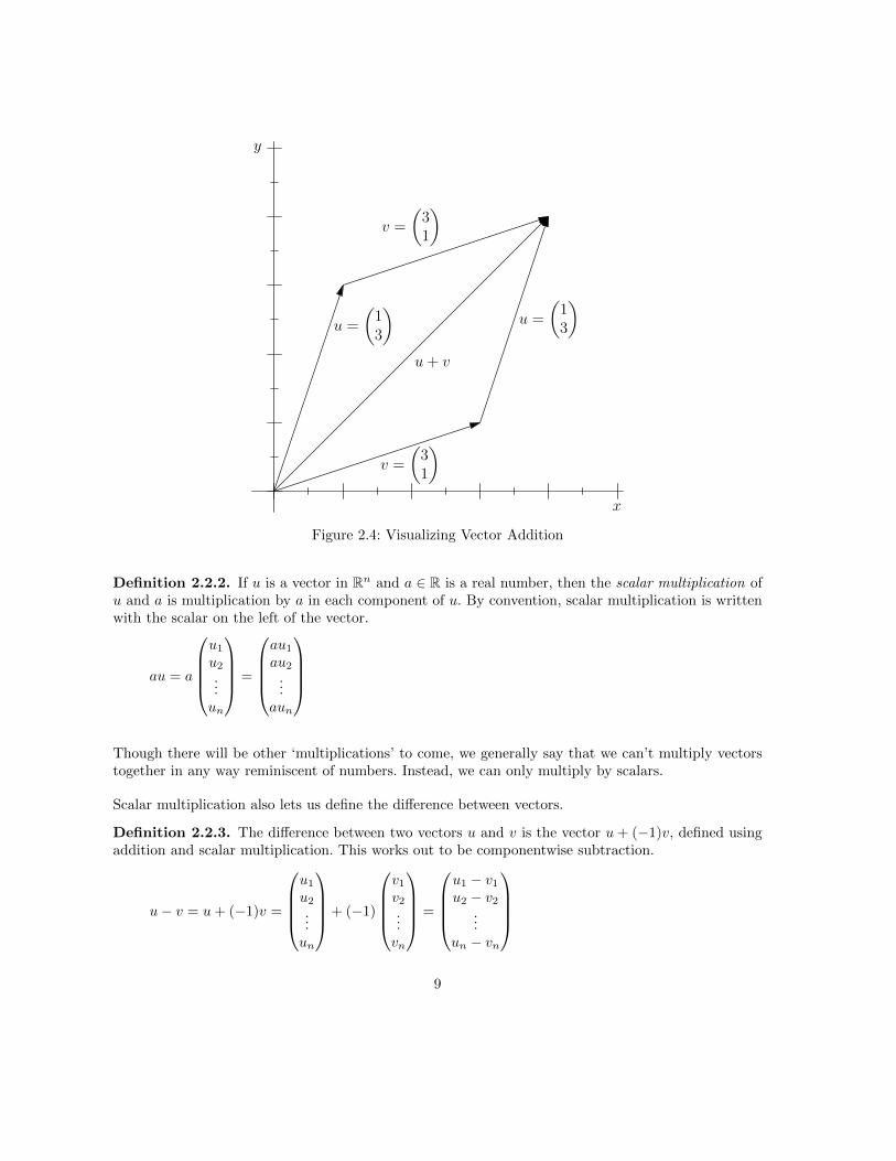
Figure 2.4: Visualizing Vector Addition

Definition 2.2.2. If u is a vector in Rn and a ∈ R is a real number, then the scalar multiplication ofu and a is multiplication by a in each component of u. By convention, scalar multiplication is writtenwith the scalar on the left of the vector.

au = a

u1u2...un

=

au1au2

...aun

Though there will be other ‘multiplications’ to come, we generally say that we can’t multiply vectorstogether in any way reminiscent of numbers. Instead, we can only multiply by scalars.

Scalar multiplication also lets us define the difference between vectors.

Definition 2.2.3. The difference between two vectors u and v is the vector u+ (−1)v, defined usingaddition and scalar multiplication. This works out to be componentwise subtraction.

u− v = u+ (−1)v =

u1u2...un

+ (−1)

v1v2...vn

=

u1 − v1u2 − v2

...un − vn

9

y

x

u =

(12

)

2u =

(24

)

14u =

(1412

)

−u =

(−1−2

)

−2u =

(−2−4

)

Figure 2.5: Visualizing Scalar Multiplication

Definition 2.2.4. Given a set of scalars (such as R), whenever we find a mathematical structure whichhas the two properties of addition and scalar multiplication, we call the structure linear. Rn is a linearspace, because vectors allow for addition and scalar multiplication.

Definition 2.2.5. The length of a vector u in Rn is written |u| and is given by a generalized form ofthe Pythagorean rule for right triangles.

|u| =√u21 + u22 + . . .+ u2n

This length is also called the norm of the vector. A vector of length one is called a unit vector.

If we think of vectors as directions from the origin towards a point, this definition of length gives exactlywhat we expect: the physical length of that arrow in R2 and R3. Past R3, we don’t have a naturalnotion of length. This definition serves as a reasonable generalization to R4 and higher dimensionswhich we can’t visualize. Note also that |u| = 0 only if u is the zero vector. All other vectors havepositive length.

Often the square root is annoying and we find it convenient to work with the square of length.

|u|2 = u21 + u22 + . . .+ u2n

The notions of length and difference allow us to define the distance between two vectors.

10

y

x

u =

(14

)

v =

(42

)

|v − u| =√32 + (−2)2 =

√13

v − u =

(3−2

)

Figure 2.6: Visualizing Distance Between Vectors

Definition 2.2.6. The distance between two vectors u and v in Rn is the length of their difference:|u− v|.

You can check from the definition that |u − v| = |v − u|, so distance doesn’t depend on which comesfirst. If |·| were absolute value in R, this definition would match the notion of distance between numberson the number line.

2.3 The Dot Product

Earlier we said that we can’t multiply two vectors together. However, there are operations similar tomultiplication. The following operations multiplies two vectors, but the result is a scalar instead ofanother vector.

11

Definition 2.3.1. The dot product or inner product or scalar product of two vectors u and v is givenby the following formula.

u · v =

u1u2...un

·

v1v2...vn

= u1v1 + u2v2 + . . .+ unvn

We can think of the dot product as a scalar measure of the similarity of direction between the twovectors. If the two vectors point in a similar direction, their dot product is large, but if they point invery different directions, their dot product is small. However, we already have a measure, at least inR2, of this difference: the angle between two vectors. Thankfully, the two measures of difference agreeand the dot product can be expressed in terms of angles.

Definition 2.3.2. The angle θ between two non-zero vectors u and v in Rn is given by the equation

cos θ =u · v|u||v|

This matches with the definition of angles in R2 and R3, which we can visualize. However, this servesas a new definition for angles between vectors in all Rn when n ≥ 4. Since we can’t visualize thosespaces, we don’t have a way of drawing angles and calculating them with conventional trigonometry.This definition allows us to extend angles in a completely algebraic way.

Definition 2.3.3. Two vectors u and v in Rn are called orthogonal or perpendicular or normal ifu · v = 0.

There are many pairs of orthogonal vectors. Thinking of the dot product as a multiplication, we haveuncovered a serious difference between the dot product and conventional multiplication of numbers. If

a, b ∈ R then ab = 0 implies that one of a or b must be zero. For vectors, we can have(

10

)·(

01

)= 0 even

though neither factor in the product is the zero vector. This is a great example of differing algebraicstructure. Abstractly, when we have a multiplication and a zero opject, two non-zero objects a and bwhich satisfy ab = 0 are called zero divisors. One of the most important properties of ordinary numbersis that there are no zero divisors. Other algebraic structures, such as vectors with the dot product,may have many zero divisors.

Now that we have some operations, it is useful to see how the various operations interact. The followinglist shows some interactions between addition, scalar multiplication, length and the dot product. Someof these are easy to establish from the definition and some take more work.

Proposition 2.3.4. Let u, v, w be vectors in Rn and let a be a scalar in R.

u+ v = v + u Commutative Law for Vector Additiona(u+ v) = au+ av Distributive Law for Scalar Multiplication

u · v = v · u Commutative Law for the Dot Productu · u = |u|2

u · (v + w) = u · v + u · w Distributive Law for the Dot Productu · (av) = (au) · v = a(u · v)|u+ v| ≤ |u|+ |v| Triangle Inequality|au| = |a||u|

12

y

x

u

v

v − u

θ

|v − u|2 = |u|2 + |v|2 − 2|u||v| cos θ

Figure 2.7: The Cosine Law

The last line deserves some attention for the notation. When we write |a||u|, |a| is an absolute value ofa real number and |u| is the length of a vector. The fact that they have the same notation is frustrating,but these notations are conventional.

All of these identities can be established by proof. For example, here is a proof for the triangle inequality,using some of the other properties. In the fifth step, we use the fact that cos θ ≤ 1 for any angle.

|u+ v|2 = (u+ v) · (u+ v)

= u · u+ v · v + u · v + v · u= u · u+ v · v + 2u · v= |u|2 + |v|2 + 2|u||v| cos θ

≤ |u|2 + |v|2 + 2|u||v|= (|u|+ |v|)2

|u+ v|2 ≤ (|u|+ |v|)2|u+ v| ≤ |u|+ |v|

In R2, norms and dot products allow us to recreate some well-known geometric constructions. For

13

example, now that we have lengths and angles, we can state the cosine law in terms of vectors.

|u− v|2 = |u|2 + |v|2 − 2|u||v| cos θ = |u|2 + |v|2 + 2u · v

The proof of the cosine law can now be reduced to manipulations of norms and dot-products of vectors.

|u− v|2 = (u− v) · (u− v) = u · u+ v · v − 2|u||v| = |u|2 + |v|2 − 2|u||v| cos θ

2.4 The Cross Product

The dot product is an operation which can be performed on any two vectors in Rn for any n ≥ 1. Thereare no other conventional products that work in all dimensions. However, there is a special productthat works in three dimensions.

Definition 2.4.1. Let u =

u1u2u3

and v =

v1v2v3

be two vectors in R3. The cross product of u and v is

written u× v and defined by this formula:

u× v =

u2v3 − u3v2u3v1 − u1v3u1v2 − u2v1

The cross product differs from the dot product in several important ways. First, it produces a newvector in R3, not a scalar. For this reason, when working in R3, the dot product is often refered to as thescalar product and the cross product as the vector product. Second, the dot product measures, in somesense, the similarity of two vectors. The cross product measures, in some sense, the difference betweentwo vectors. The cross product has greater magnitude if the vectors are closer to being perpendicular.If θ is the angle between u and v, the dot product was expressed in terms of cos θ. This measuressimilarity, since cos 0 = 1. There is a similar identity for the cross product:

|u× v| = |u||v| sin θ

This identity tells us that the cross product measures difference in direction, since sin 0 = 0. Inparticular, this tells us that |u × u| = 0, implying that u × u = 0 (the zero vector is the only vectorwhich has zero length). This is another very new and strange property of a multiplication: everythingsquares to produce zero. The cross product is obviously very different from multiplication of scalars.

We can also calculate the following:

u · (u× v) =

u1u2u3

·

u2v3 − u3v2u3v1 − u1v3u1v2 − u2v1

= u1u2v3 − u1u3v2 + u2u3v1 − u2u1v3 + u3u1v2 − u3u2v1 = 0

14

A similar calculation shows that v · (u× v) = 0. Since a dot product of two vectors is zero if and only ifthe vectors are perpendicular, the vector v× u is perpendicular to both u and v. (This property turnsout to be very useful for describing planes later in these notes.)

Finally, an easy calculation from the definition shows that u × v = −(v × u). So far, multiplicationof scalars and the dot product of vectors have not depended on order. The cross product is one ofmany products in mathematics which depends on order. If we change the order of the cross product,we introduce a negative sign. Products which do not depend on the order of the factors, such as mul-tiplication of scalars and the dot product of vectors, are called commutative products. Products wherechanging the order of the factors introduces a negative sign are caled anti-commutative products. Thecross product is an anti-commutative product. Other products which have neither of these propertiesare called non-commutative.

An important application of the cross product is describing rotational movtion. Linear mechanicsdescribes the motion of an object through space but rotational mechanics describes the rotation ofan object independanly of its movement through space. A force on an object can cause both kindsof movement, obviously. This table summarizes the parallel questions of linear motion and rotationalmotion in R3:

Linear Motion Rotational MotionStraight line in a vacuum Continual spinning in a vacuumDirection of motion Axis of spinForce TorqueMomentum Angular MomentumMass (resistance to motion) Moment of Intertia (resistance to spin)Velocity Frequency (Angular Velocity)Acceleration Angular Acceleration

How do we describe torque? If there is a linear force applied to an object which can only rotate aroundan axis, and if the linear force is applied at a distance r from the axis, we can think of the force F andthe distance r as vectors. The torque is then τ = r × F . Notice that |τ | = |r||F | sin θ, indicating thatlinear force perpendicular to the radius gives the greatest angular acceleration. That makes sense. IfF and r are colinear, that means we are pushing directly along the axis and no rotation can occur.

The use of cross products in rotational dynamics is extended in many interesting ways. In fluid dy-namics, local rotational products of the fluid result in turbulence, helicity, vorticity and similar effects.Tornadoes and hurricanes are particularly extreme examples of vortices and helices in the fluid whichis the atmosphere. All the descriptions of the force and motion of these vortices involve cross productsin the vectors describing the fluid.

2.5 Local Direction Vectors

We’ve already spoken about the distinction between elements of Rn as points and vectors. There isanother important subtlety that shows up all throughout vector geometry. In addition to thinking of

15

y

x

(22

)

Local

(10

)

Local

(10

)

Figure 2.8: Local Direction Vectors

vectors as directions starting at the origin, we can think of them as directions starting anywhere inRn. We call these local direction vectors.

For example, at the point(

22

)in R2, we could think of the local directions

(10

)or

(01

). These are not

directions starting from the origin, but starting from(

22

)as if that were the origin.

Using vectors to specify local directions is a particularly useful tool. A standard example is cameralocation in a three dimensional virtual environment. First, you need to know the location of thecamera, which is an ordinary vector starting from the origin. Second, you need to know what directionthe camera is point, which is a local direction vector which treats the camera location as the currentorigin.

One of the most difficult things about learning vector geometry is becoming accustomed to localdirection vectors. We don’t always carefully distinguish between vectors at the origin and local directionvectors; often, the difference is implied and it is up to the reader/student to figure out how the vectorsare being used.

16

y

x

(14

)

(41

)

Proj(41

)(14

)

Perp(41

)(14

)

Figure 2.9: Projection and Perpendicular Vectors

2.6 Projections

For any vector v, every vector u can be decomposed into

Definition 2.6.1. Let u and v be two vectors in Rn. The projection of u onto v is a scalar multipleof the vector v given by the following formula.

Projvu =

(u · v|v|2

)v

Note that the bracketted term involves the dot product and the norm, so it is a scalar. Therefore, theresult is a multiple of the vector v. Projection is best visualized as the shadow of the vector u on thethe vector v.

Definition 2.6.2. Let u and v be two vectors in Rn. The part of u which is perpendicular to v is givenby the following formula.

Perpvu = u− Projvu

17

We can rearrange this to be

u = Projvu+ Perpvu

For any vector v, every vector u can be decomposed into a sum of two unique vectors: one in thedirection of v and one perpendicular to v. If u and v are already perpendicular, then the projectionterm is the zero vector. If u is a multple of v, then the perpendicular term is the zero vector. We thinkof this decomposition as capturing two pieces of the vector u: the part that aligns with the directionof v and the part that has nothing to do with the direction of v.

The following relationship between projections and angles is easy to prove from the definitions.

Proposition 2.6.3. If u and v are vectors in Rn and θ is the angle between them, then |Projvu| =|u| cos θ.

2.7 Objects in Rn

Now that we have defined vectors, we want to investigate more complicated objects in Rn. The majorobjects for the course work (linear and affine subspaces) will be defined in the following section. Inthis section, we take a short detour to discover how familiar shapes and solids extend into higherdimensions. I’ll use the standard term polyhedron (plural polyhedra) to refer to a straight-edged objectin any Rn.

2.7.1 Cubes

Let’s start with square objects. The ‘square’ object in RR is the interval [0, 1]. It can be defined bythe inequality 0 ≤ x ≤ 1 for x ∈ R. In R2, the square object is the just the (solid) square. It is all

vectors(xy

)such that 0 ≤ x ≤ 1 and 0 ≤ y ≤ 1. The square can be formed by taking two intervals and

connecting the matching vertices. It has four vertices and four edges.

In R3, the square object is the (solid) cube. It is all vectors

xyz

, such that each coordinate is in the

interval [0, 1]. It can also be seen as two squares with matching vertices connected. Two square giveseight vertices. Eight square edges plus four connecting edges gives the twelve edges of the cube. It alsohas six square faces.

Then we can simply keep extending. In R4, the set of all vectors

xyzw

where all coordinates are in

the interal [0, 1] is called the hypercube or 4-cube. It can be seen as two cubes with pairwise edgesconnected. The cubes each have eight vertices, so the 4-cubes has sixteen vertices. Each cube has 12

18

edges, and their are 8 new connecting edges, so the 4-cube has 32 edges. It has 24 faces and 8 cells. Acell (or 3-face) here is a three dimensional ‘edge’ of a four (or higher) dimensional object.

There is an n-cube in each Rn, consisting of all vectors where all components are in the interval [0, 1].Each can be constructed by joining two copies of a lower dimensional (n− 1)-cube with edges betweenmatching vertices. Since there are two copies with no other new edges, vertices double with each step.The grow of edges, faces, cells and other k-faces is much trickers to determine. (Edges more thandouble, since we add connecting edges in each step) Here is a chart of the number of parts of lowdimensional cubes.

Dimension Vertices Edges Faces Cells 4-Cells 5-Cells 6-Cells 7-Cells0 1 0 0 0 0 0 0 01 2 1 0 0 0 0 0 02 4 4 1 0 0 0 0 03 8 12 6 1 0 0 0 04 16 32 24 8 1 0 0 05 32 80 80 40 10 1 0 06 64 192 240 160 60 12 1 07 128 448 672 560 280 84 14 18 256 1024 1792 1792 1120 448 112 16

2.7.2 Spheres

Spheres are, in some way, the easiest objects to generalize. Spheres are all things in Rn which are exactlyone unit of distance from the origin. The ‘sphere’ in R is just the points −1 and 1. The ‘sphere’ in R2 isthe circle x2 +y2 = 1. The sphere in R3 is the conventional sphere, with equation x2 +y2 +z2 = 1. Thesphere in R4 has equation x2 +y2 + z2 +w2 = 1. The sphere in Rn has equation x21 +x22 + . . .+x2n = 1.For dimensional reasons, since the sphere is usually considered to be a hollow objects, the sphere inRn is called the (n − 1)-sphere. That means the circle is the 1-sphere and the conventional sphere isthe 2-sphere.

A sphere relate to the previous dimension by looking at slices. Any slice of a sphere produces a circle.Likewise, any slice of a 3-sphere produces a 2-sphere.

2.7.3 Simplicies

Though the cubes are more intuitively comfortable, the simplices may be the most fundamentalstraight-line polyhedra. I’ll define them without specifying their vector definition in Rn, since it isslightly more technical than necessary. The 1-simplex is a line segment. The 2-simplex is an equilateraltriangle. It is formed from the 1-simplex by adding one new vertex and drawing edges to the existingvertex such that all edges have the same length. The 3-simplex is a tetrahedron. Again, it is formed by

19

adding one new vertex and drawing lines to all existing vertices such that all line (new and old) havethe same length.

This process extends into higher dimensions. In each stage a new vertex is added and edges connect itto all previous vertices, such that all edges have the same length. The growth of vertices is simple, sinceone is added in each dimension. The growth of edges is not to difficult, since n are added in dimensionn. The growth of other faces is tricker, but summarized in this table. The table is just Pascal’s triangle,for those who know it.

Dimension Vertices Edges Faces Cells 4-Cells 5-Cells 6-Cells 7-Cells0 1 0 0 0 0 0 0 01 2 1 0 0 0 0 0 02 3 3 1 0 0 0 0 03 4 6 4 1 0 0 0 04 5 10 10 5 1 0 0 05 6 15 20 15 6 1 0 06 7 21 35 35 21 7 1 07 8 28 56 70 56 28 8 18 9 36 84 126 126 84 36 9

2.7.4 Cross-Polytope

The only other family of regular solids which extends to all dimensions are called the cross-polytopes.They are, in some way, the diamonds to balance the squares of the cube. In R2, the cross-polytope is

the diamond with vertices(

10

),(−10

),(

01

), and

(0−1

). In each dimension, two vertices are added at ±1 in

the new axis direction, and edges are added connecting the two new vertices to each existing vertex.

In R3, the cross-polytope is the octahedron, with vertices

100

,

−100

,

010

,

0−10

,

001

, and

00−1

. In higher

dimensions, the vertices are all vectors with ±1 in one component and zero in all other components.Each vertex is connected to all other vertices except its opposite.

Here is the table for cross-polytopes.

Dimension Vertices Edges Faces Cells 4-Cells 5-Cells 6-Cells 7-Cells1 2 0 0 0 0 0 0 02 4 4 0 0 0 0 0 03 6 12 8 0 0 0 0 04 8 24 32 16 0 0 0 05 10 40 80 80 32 0 0 06 12 60 160 240 192 64 1 07 14 84 280 560 672 448 128 18 16 112 448 1120 1792 1792 1024 256

20

If we look carefully, we can see that the vertices and the (n−1)-faces of the cubes and the cross-polytopeshave the same sequences. We can also notices other symmetries in the tables. This symmetry comesfrom the fact that the cube and the cross-polytopes are dual. In R3, this can be seen by labeling thecentre of each face of the cube with a vertex and connecting the vertices to make the octahedron.The opposite process for the octahedro recovers the cube. The simplex, should you be wondering, ifself-dual.

2.7.5 Other Platonic Solics

A regular polyhedron is one where all edges, faces, cells, n-cells are the same size/shape and, in addition,the angles between all the edges, faces, cells, n-cells are also the same whever the various objects meet.In addition, the polyhedron is called convex if all angles are greater that π

2 radians. The study of convexregular polyhedra is an old and celebrated part of mathematics.

In R2, there are infinitely many convex regular polyhedra: the regular polygons with any numberof sides. In R3, in addition to the cube, tetrahedron and octahedron, there are only two others: thedodecahedron and the icosahedron. These were well known to the ancient Greeks and are called thePlatonic Solids.

The three families (cube, tetrahedron, cross-polytope) extend to all dimensions, but the dodecahedronand icoahedron are particular to R3. It is a curious and fascinating question to ask what other special,unique convex regular polyhedra occur in higher dimesions.

In R4, there are three others. They are called the 24-cell, the 120-cell and 600-cell, named for thenumber of 3-dimensional cells they contain (the same way the 4-cubes contains 8 3-cubes). The 24-cellis built from 24 octahedral cells. The 120-cell is built from dodecahedral cells and the 600-cell is builtfrom tetrahedral cells. The 120-cell, in some ways, extends the dodecahedron and the 600-cell extendsthe icosahedron. The 24-cell is unique to R4.

It is an amazing theorem of modern mathematics that in dimensions higher that 4, there are no regularpolyhedra other than the three families. Neither the icosahedron nor the dodecahedron extend, andthere are no other erratic special polyhedra found in any higher dimension.

2.8 Linear and Affine Subspaces

In addition to vectors, we want to consider various geometric objects that live in Rn. Since this is linearalgebra, we will be restricting ourselves to flat objects.

Definition 2.8.1. A linear subspace of Rn is a non-empty set of vectors L such that two propertieshold:

• If u, v ∈ L then u+ v ∈ L.

21

• If u ∈ L and a ∈ R then av ∈ L.

These were the two basic operations on Rn: we can add vectors and we can multiply by scalars. Linearsubspaces are just subsets where we can still perform both operations and remain in the subset.

Geometrically, vector addition and scalar multiplication produce flat objects: lines, planes, and what-ever the higher-dimensions analogues are. Also, since we can take a = 0, we must have 0 ∈ L. So linearsubspaces can be informally defined as flat subsets which include the origin.

Definition 2.8.2. An affine subspace of Rn is a non-empty set of vectors A which can be described asa sum v + u where v is a fixed vector and u is any vector in some fixed linear subspace L. With someabuse of notation, we can write this as

A = u+ L

We think of affine subspaces as flat spaces that may be offset from the origin. The vector u is calledthe offset vector. Affine spaces include linear spaces, since we can also take u to be the zero vector andhave A = L. Affine objects are the lines, planes and higher dimensional flat objects that may or maynot pass through the origin.

Notice that we defined both affine and linear subspaces to be non-empty. The empty set ∅ is not alinear or affice subspace.

We need ways to algebraically describe linear and affine substapces. There are two main approaches:loci and spans.

2.9 Loci

Definition 2.9.1. Consider any set of linear equations in the variables x1, x2, . . . , xn. The locus in Rnof this set of equations is the set of vectors which satisfy all of the equations. The plural of locus isloci.

In general, the equations can be of any sort. The unit circle in R2 is most commonly defined as the locusof the equation x2 + y2 = 1. The graph of a function is the locus of the equation y = f(x). However,in linear algebra, we exclude curved objects. We’re concerned with linear/affine objects: things whichare straight and flat.

Definition 2.9.2. A linear equation in variables x1, x2, . . . xn is an equation of the form

a1x1 + a2x2 + . . .+ anxn = c

where ai and c are real numbers

22

Proposition 2.9.3. Any linear or affine subspace of Rn can be described as the locus of some numberof linear equations. Likewise, any locus of any number of linear equations is either an affine subspaceof Rn or the empty set..

The best way to think about loci is in terms of restrictions. We start with all of Rn as the locus ofno equations, or of the equation 0 = 0. There are no restrictions. Then we introduce equations. Eachequation is a restriction on the available points. If we work in R2, adding the equation x = 3 restricts

us to a vertical line passing through the x-axis at(

30

). Likewise, if we were to use the equation y = 4,

we would have a horizontal line passing through the y-axis at(

04

). If we consider the locus of both

equations, we have only one point remaining:(

34

)is the only point that satisfies both equations.

In this way, each additional equation potentially adds an additional restriction and leads to a smallerlinear or affine subspace.

The general linear equation in R2 is given by the equation ax+ by = c for real numbers a, b, c. This isone restriction, so it should drop the dimension from the ambient two to one.

Definition 2.9.4. A line in R2 is the locus of the equation ax+ by = c for a, b, c ∈ R. In general, theline is affine. The line is linear if c = 0.

In R3, we can think of a general linear equation as ax+ by + cz = d for a, b, c, d ∈ R.

Definition 2.9.5. A plane in R3 is the locus of the linear equation ax+ by + cz = d. In general, theplane is affine. The plane is linear if d = 0.

If we think of a plane in R3 as the locus of one linear equation, then the important dimensional factabout a plane is not that it has dimension two but that it has dimension one less that its ambientspace R3. This is how we generalize the plane to higher dimensions.

Definition 2.9.6. A hyperplane in Rn is the locus of one linear equation: a1x1 +a2x2 + . . .+anxn = c.It has dimension n− 1. It is, in general, affine. The hyperplane is linear if c = 0.

All this discussion is pointing towards the notion of dimension. The dimension of Rn is n; it is thenumber of independent directions or degrees of freedom of movement. For subspaces, we also want awell-defined notion of dimension. So far it looks good: the restriction of a linear equation should dropthe dimension by one. Then a line in R3, which is one dimensional in a three dimensional space, shouldbe the locus of two different linear equations.

We would like the dimension of a locus to be simply determined by the dimension of the ambient spaceminus the number of equations. However, there is a problem with the naive approach to dimension. InR2, adding two linear equations should drop the dimension by two, giving a dimension zero subspace:a point. However, consider the equations 3x+ 4y = 0 and 6x+ 8y = 0. We have two equations, but the

23

second is redundant. All points on the line 3x + 4y = 0 are already satisfied by the second equation.So, the locus of the two equations only drops the dimension by one.

In R3 the equations y = 0, z = 0 and y+z = 0 have a locus which is the x axis. This is one dimensionalin a three dimensional space, so the dimension from the three equations has only dropped by two. Oneof the equations is redundant.

This problem scales into higher dimensions. In Rn, if we have several equations, it is almost impossible tosee, at a glance, whether any of the equations are redundant. We need methods to calculate dimension.Unfortunately, those methods will have to wait until later in these notes. For now, we’ll move on fromloci to the second way of describing linear and affine spaces.

2.9.1 Intersection

Definition 2.9.7. If A and B are sets, their intersection A ∩ B is the set of all points they have incommon. The intersection of affine subsets is also an affine subset. If A and B are both linear, theintersection is also linear.

Example 2.9.8. Loci can easily be understood as intersections. Consider the locus of two equations,say the example we have from R2 before: the locus of x = 3 and y = 4. We defined this directly asa single locus. However, we could just as easily think of this as the intersection of the two lines givenby x = 3 and y = 4 seperately. In this way, it is the intersection of two loci. Similarly, all loci are theintersection of planes or hyperplanes.

2.10 Spans

Definition 2.10.1. A linear combination of a set of vectors {v1, v2, . . . , vk} is a sum a1v1 + a2v2 +. . . akvk where the ai ∈ R.

Definition 2.10.2. The span of a set of vectors {v1, v2, . . . , vk}, written Span{v1, v2, . . . , vk}, is theset of all linear combinations of the vectors.

After loci, spans are the second way of defining flat objects. However, since linear combinations allowfor all the coefficients ai to be zero, spans always include the origin. Therefore, spans are always linearsubspaces. To use spans to define general affine objects, we have to add an offset vector.

Definition 2.10.3. An offset span is an affine subspace formed by adding a fixed vector u, called theoffset vector, to the span of some set of vectors.

24

Loci are built top-down, by starting with the ambient space and reducing the number of points byimposing restrictions in the form of linear equations. Their dimension, at least ideally, is the dimensionof the ambient space minus the number of equations or restrictions. Spans, on the other hand, are builtbottom-up. They start with a number of vectors and take all linear combination: more starting vectorsleads to more independent directions and a larger dimension.

In particular, the span of one non-zero vector is a line, in any Rn. That span is just the set of allmultiples of that vector. Similarly, we expect the span of two vectors to be a plane in any Rn. However,here we have the same problem as we had with loci: we may have redundant information. For example,

in R2, we could consider the span Span

{(12

),

(24

)}. We would hope the span of two vectors would be the

entire plane, but this is just the line in the direction(

12

). The vector

(24

), since it is already a multiple

of(

12

), is redundant.

The problem is magnified in higher dimensions. If we have the span of a large number of vectors in Rn,it is nearly impossible to tell, at a glance, whether any of the vectors are redundant. We would like tohave tools to determine this redundancy. As with the tool for dimensions of loci, we have to wait untila later section of these notes.

2.11 Dimension and Basis

Definition 2.11.1. A set of vectors {v1, v2, . . . , vk} in Rn is called linearly independent if the equation

a1v1 + a2v2 + a3v3 + . . .+ akvk = 0

has only the trivial solution: for all i, ai = 0. If a set of vectors isn’t linearly independent, it is calledlinearly dependant.

This may seem like a strange definition, but it algebriaclly captures the idea of independent directions.A set of vectors is linearly independent if all of them point in fundamentally different directions. Wecould also say that a set of vectors is linearly independent is no vector is in the span of the othervectors. No vector is a redundant piece of information; if we remove any vectors, the span of the setgets smaller.

In order for a set like this to be linearly independent, we need k ≤ n. Rn has only n independentdirections, so it is impossible to have more than n linearly independent vectors in Rn.

Definition 2.11.2. Let L be a linear subspace of Rn. Then L has dimension k if L can be written asthe span of k linearly independent vectors.

Let A be an affine subspace of Rn and write A as A = u + L for L a linear subspace and u a offsetvector. Then A has dimension k if L has dimension k.

25

This is the proper, complete definition of dimension for linear and affine spaces. It solves the problem ofredundant information (either redundant equations for loci or redundant vectors for spans) by insistingon a linearly independent spanning set.

Definition 2.11.3. Let L be a linear subspace of Rn. A basis for L is a minimal spanning set; thatis, a set of linearly independent vectors which span L.

Since a span is the set of all linear combinations, we can think of a basis as as way of writing thevectors of L: every vector in L can be written as a linear combination of the basis vectors. A basisgives a nice way to account for all the vectors in L.

Linear subspaces have many (infinitely many) different bases. There are some standard choices.

Definition 2.11.4. The standard basis of R2 is composed of the two unit vectors in the positive xand y directions.

e1 =

(10

)e2 =

(01

)

The standard basis of R3 is composed of the three unit vectors in the positive x, y and z directions.

e1 =

100

e2 =

010

e3 =

001

The standard basis of Rn is composed of vectors e1, e2, . . . , en where ei has a 1 in the ith componentand zeroes in all other components. ei is the unit vector in the positive ith axis direction.

2.12 Standard Forms

Loci can also be defined via dot products. Consider, again, the general linear equation in Rn:

a1u1 + a2u2 + . . .+ anun = c

Let’s think of the variables ui as the components of a variable vector u ∈ Rn. We also have n scalarsai which we can treat as a constant vector a ∈ Rn.

Then we can re-write the linear equation as:

a1u1 + a2u2 + . . .+ anun =

a1a2...an

·

u1u2...un

= a · u = c

26

In this way, a linear equation specifies a certain dot product (c) with a fixed vector (a). A plane in R3

is given by the equation

xyz

·

a1a2a3

= c. The plane is precisely all vectors whose dot product with the

vector

a1a2a3

is the fixed number c.

If c = 0, then we get

xyz

·

a1a2a3

= 0. A linear plane is the set of all vectors which are perpendicular to a

fixed vector

a1a2a3

.

Definition 2.12.1. Let P be a plane in R3 determined by the equation

xyz

·

a1a2a3

= c. The vector

a1a2a3

is called the normal to the plane.

Let H be a hyperplane in Rn determined by the equation

u · a =

u1u2...un

·

a1a2...an

= c

The vector a is called the normal to the hyperplane.

If c = 0, the plane or hyperplane is perpendicular to the normal. This notion of orthogonality stillworks when c 6= 0. In this case, the normal is a local perpendicular direction from a point on the affineplane. Treating any such point as a local origin, the normal points in a direction perpendicular to allthe local direction vectors which lie on the plane.

Now we can build a general process for finding the equation of a plane in R3. Any time we have apoint p on the plane and two local direction vectors u and v which remain on the plane, we can finda normal to the plane by taking u× v. Then we can find the equation of the plane by taking the dotproduct p · (u× v) to find the constant c. We get the equation of the plane.

xyz

· (u× v) = c

If we are given three points on a plane (p, q and r), then we can use p as the local origin and constructthe local direction vectors as q − p and r − p. The normal is (q − p) × (r − p). In this way, we canconstruct the equation of a plane given three points or a single point and two local directions.

27

Chapter 3

Systems of Linear Equations

3.1 Definitions

We now move into the algebraic roots of linear algebra, as opposed to the geometric perspective westarted with. A major problem in algebra is solving systems of equations: given several equations inseveral variables, can we find values for each variable which satisfy all the equations. In general, thesecan be any kind of equations.

Example 3.1.1.

x2 + y2 + z2 = 3

xy + 2xz − 3yz = 0

x+ y + z = 3

This system is solved by

xyz

=

111

. When substitued in the equations, these values satisfy all three.

No other triples satisfies, so this is a unique solution.

In general, solving systems of equations is a very difficult problem. There are two initial techniques,which are usually taught in high-school mathematics: isolating and replacing variables; or performingarithmetic with the equations themselves. Both are useful techniques. However, when the equationsbecome quite complicated, both methods can fail. In that case, it is a problem that can only beapproached with computerized approximation methods. The methodology of these algorithms is awhole branch of mathematics in itself. We are going to restrict ourselves to a class of systems which ismore approchable: systems of linear equations. Recall the definition of a linear equation.

28

Definition 3.1.2. A linear equation in the variables x1, x2 . . . , xn is a equation of the form

a1x1 + a2x2 + . . .+ anxn = c

where ai and c are real numbers.

Given a fixed set of variables x1, x2, . . . , xn, we want to consider systems of linear equations (and onlylinear equations) in those variables. While much simpler than the general case, this is still a commonand useful type of system to consider. Such systems also work well with arithmetic solution techniques,since we can add two linear equations together and still have a linear equation.

This turns out to be the key idea: we can do arithmetic with linear equations. Specifically, there arethree things we can do with a system of linear equation. These three techniques preserve the solutions,that is, they don’t alter the values of the variables that solve the system.

These three operations are:

• Multiple a single equation by a (non-zero) constant. (Multiplying both sides of the equation, ofcourse).

• Change the order of the equations.

• Add one equation to another.

If we combine the first and third, we could restate the third as: add a multiple of one equation toanother. In practice, we often think of the third operation this way.

3.2 Matrix Representation of Systems

We could work with the equations directly and use the three techniques. We would find that with carefulapplication of those techniques, we could always solve the system. However, the notation becomescumbersome for large systems. Therefore, we want a method to encode the information in a nicelyorganized way. We can use matrices.

Consider a general system with m equations in the variables x1, x2, . . . , xn, where aij and ci are realnumbers.

a11x1 + a12x2 + . . . a1nxn = c1

a21x1 + a22x2 + . . . a2nxn = c2

. . .

am1x1 + am2x2 + . . . amnxn = cm

29

We encode this as an extended matrix by taking the aij and the ci as the matrix coefficients. We dropthe xi, keeping track of them implicitly by their positions in the matrix. The result is a m × (n + 1)extended matrix where the vertical line notes the position of the equals sign in the origin equation.

a11 a12 . . . a1n c1a21 a22 . . . a2n c2. . . . . . . . . . . . . . .a11 a12 . . . a1n c1

Example 3.2.1.

−x+ 3y + 6z = 1

2x+ 2y + 2z = −6

5x− 5y + z = 0

We transfer the coefficient into the matrix representation.−1 3 6 12 2 2 −65 −5 1 0

Example 3.2.2.

−3x− 10y + 15z = −34

20x− y + 19z = 25

32x+ 51y − 31z = 16

We transfer the coefficient into the matrix representation.−3 −10 15 −3420 −1 19 2532 51 −31 16

Example 3.2.3. If we are working with three or more variables, sometimes not all equations mentioneach variable.

x− 2z = 0

2y + 3z = −1

−3x− 4y = 9

This system is clarified by adding the extra variables with coefficient 0.

x+ 0y − 2z = 0

0x+ 2y + 3z = −1

−3x− 4y + 0z = 9

30

Then it can be clearly encoded as a matrix.

1 0 −2 00 2 3 −1−3 −4 0 9

In this way we can change any system of linear equations into a extended matrix (with one column afterthe vertical line), and any such extended matrix into a system of equations. The columns representthe variables. In the examples above, we say that the first column is the x column, the second is the ycolumn, the third if the z column, and the column after the vertical line is the column of constants.

3.3 Row Operations and Gaussian Elimination

We had three arithmetic operations on systems of equations. Now that we have encoded systems asmatrices, we need to understand the equivalent operations. Each equation in the system gives a row inthe matrix; therefore, equation operations become row operations.

• Multiply an equation by a non-zero constant =⇒ multiply a row by a non-zero constant.

• Change the order of the equations =⇒ exchange two rows of a matrix.

• Add (a multiple of) an equation to another equation =⇒ add (a multiple of) one row to anotherrow.

Since the original operation didn’t change the solution of a system of equations, the row operation onmatrices preserve the solution of the associated system.

Example 3.3.1. This example shows the encoding of a direction solution.

1 0 0 −30 1 0 −20 0 1 8

The system has three columns before its vertical line, therefore it corresponds to a system of equationin x, y, z. If we translate this back into equations, we get the following system.

x+ 0y + 0z = −3

0z + y + 0z = −2

0x+ 0y + z = 8

Removing the zero terms gives x = −3, y = −2 and z = 8. This equation delivers its solution directly:no work is necessary. We just read the solution off the page.

31

Now we can state our approach to solving linear systems. We want to translate a system into a matrix.We want to use row operations (which don’t change the solution at all) to turn the matrix into onesimilar to the previous example: one where we can just read off the solution. Row operations will alwaysbe able to accomplish this. However, we need to be more specific about the form of the matrix.

Definition 3.3.2. A matrix is a reduced row-echelon matrix, or is said to be in reduced row-echelonform, if the following things are true:

• The first non-zero entry in each row is one. (A row entirely of zeros is fine). These entries arecalled leading ones.

• Each leading one is in a column where all the other entries are zero.

We shall see that as long as an extended matrix is in reduced row-echelon form, we can always directlyread off the solution to the system. Therefore, our goal is take any extended matrix and change it,using only row operations, into reduced row-echelon form.

The general process is called Guassian elimantion or row reduction.

• Take the first row which has a non-zero entry in the first column. (Often we exchange this rowwith the first, so that we are working on the first row). If there are rows of all zeros, then weleave them alone.

• Multiply by a constant to get a leading one in this row.

• Now that we have a leading one, we want to clear all the other entries in the column. Thererfore,we add multiples of the row with the leading one to the other rows, one by one, to make thosecolumn entries zero.

• That produces a column with a leading one and all other entries zero. Then we proceed to thenext column and repeat the process all over again.

3.4 Solution Spaces and Free Parameters

Definition 3.4.1. If we have a system of equations in the variables x1, x2, . . . , xn, the set of values forthese variables which satisfy all the equations is called the solutions space of the system. Since eachset of values is a vector, we think of the solution space as a subset of Rn. For linear equations, this willalways be a affine subset. If we have encoded the system of equations in an extended matrix, we canrefer to the solution space of the matrix instead of the system.

Definition 3.4.2. Since solution spaces are affine, they can be written as u + L where u is a fixedoffset vector and L is a linear space. Since L is linear, it has a basis v1, v2, . . . vk and any vector in Lis a linear combination of the vi. We can write any and all solutions to the system in the followingfashion (where a i ∈ R).

u+ a1v1 + a2v2 + a3v3 + . . .+ akvk

In such a description of the solution space, we call the ai free parameters. One of our goals in solvingsystems is to determine the number of free parameters for each solution space.

32

Let’s return to the example at the start of this section to understand how we read solutions fromreduced row-echelon matrices.

1 0 0 −30 1 0 −20 0 1 8

This example is the easiest case: we have a leading one in each row and column left of the horizontalline, and we just read off the solution, x = −3, y = −2 and z = 8. Several other things can happen,though, which we will also explain by examples.

Example 3.4.3. We might have a row of zeros:

1 0 0 −30 1 0 −20 0 1 80 0 0 0

This row of zeros doesn’t actually change the solution at all: it is still x = −3, y = −2 and z = 8. Thelast line just corresponds to an equation which says 0x + 0y + 0z = 0 or just 0 = 0 which is alwaystrue. Rows of zeros arise when there were originally redundant equations.

Example 3.4.4. We might have a column of zeros. Consider something similar to the previous exam-ples, but now in four variables w, x, y, z. (In that order, so that the first column is the w column, thesecond is the x column, and so on).

1 0 0 0 −30 1 0 0 −20 0 1 0 8

Here the translation gives w = −3, x = −2 and y = 8 but they say nothing about z. A column of zeroscorresponds to a free variable: any value of z solves the system as long as the other variables are set.

Example 3.4.5. The columns of a free variables need not contain all zeros. The following matrix isstill in reduced row-echelon form:

1 0 0 2 −30 1 0 −1 −20 0 1 −1 8

Reduced row-echelon form needs a leading one in each non-zero row, and all other entries in a columnwith a lead one must be zero. This matrix satisfies all the conditions. The fourth column correspondsto the z variable, but lacks a leading one. Any column lacking a leading one corresponds to a freevariable. This translates to the system:

w + 2z = −3

x− z = −2

y − z = 8

33

If we move the z terms over, we get:

w = −2z − 3

x = z − 2

y = z + 8

z = z

We’ve added the last equation, which is trivial to satisfy, to show how all the terms depend on z. Thismakes it clear that z is a free variable, since we can write the solution as follows:

wxyz

=

−3−280

+ z

−2111

Any choice of z will solve this system. If we want specific solutions, we take specific values of z. Forexample, if z = 1, these equations give w = −5, x = −1 and y = 9. We see this solutions as an offsetspane, where the columns of constants is the offset and the parameter gives the span.

Example 3.4.6. We can go further. The following matrix is also in reduced row-echelon form:

(1 0 3 2 −30 1 −1 −1 −2

)

Here, both the third and the fourth columns have no leading one, therefore, both y and z are freevariables. Translating this system gives

w = −3y − 2z − 3

x = y + z − 2

y = y

z = z

wxyz

=

−3200

+ y

−3110

+ z

−2101

Any choice of y and z gives a solution. For example, if y = 0 and z = 1 then w = −5 and x = −1completes a solution. Since we have all these choice, any system with a free variable has infinitely manysolutions.

Example 3.4.7. Finally, we can also have a reduced row-echelon matrix of this form:

1 0 0 −30 1 0 −20 0 1 80 0 0 1

34

The first three row translate fine. However, the third row translates to 0x + 0y + 0z = 1 or 0 = 1.Obviously, this can never be satisfied. Any row which translates to 0 = 1 leads to a contradiction: itmeans that the system has no solutions, since we can never satisfy an equation like 0 = 1.

We summarize the three possible situations for reduced row-echelon matrices.

• If there is a row which translates to 0 = 1, then there is a contradiction and the system has nosolutions. This overrides any other information: whether or not there are free variables elsewhere,there are still no solutions.

• If there are no 0 = 1 rows and all columns left of the vertical line have leading ones, then thereis a unique solution. There are no rows with free variables, and each variable has a value whichwe can read directly from the matrix.

• If there are no 0 = 1 rows and there is at least one column left of the vertical line without aleading one, then each such column represents a free variable. The remaining variables can beexpressed in terms of the free variables and any choices of the free variables leads to a solution.There are infinitely many solutions. The solutions space can always be expressed as a offset span.

In particular, note that there are only three basic cases for the number of solutions: none, one, orinfinitely many. No linear system has exactly two or exactly three solutions.

3.5 Dimensions of Spans

We can now created the desired techniques to solve the dimension problems that we presented earlier.For loci and spans, we didn’t have a way of determining what information was redundant. Row-reduction of matrices gives us the tool we need.

Definition 3.5.1. Let A be a m×n matrix. The rank of A is the number of leading ones in its reducedrow-echelon form.

Given some vectors {v1, v2, . . . , vk}, what is the dimension of Span{v1, v2, . . . , vk}? By definition, it isthe number of linearly independent vectors in the set. Now we can test for linearly independent vectors.

Proposition 3.5.2. Let {v1, v2, . . . , vk} be a set of vectors in Rn. If we make these vectors the rowsof a matrix A, then the rank of the matrix A is the number of linearly independent vectors in theset. Moreover, if we do the row reduction without exchanging rows (which is always possible), then thevectors which correspond to rows with leading ones in the reduced row-echelon form form a maximallinearly independent set, i.e., a basis. Any vector corresponding to a row without a leading one is aredundant vector in the span. The set is linearly independent if and only if the rank of A is k.

35

3.6 Dimensions of Loci

Similarly, we can use row-reduction of matrices to find the dimensions of a loci. In particular, we willbe able to determine if any of the equations were redundant. Recall that we described any affine orlinear subspace of Rn as the locus of some finite number of linear equations. That is, the locus is theset of points that satisfy a list of equations.

a11x1 + a12x2 + . . . a1nxn = c1

a21x1 + a22x2 + . . . a2nxn = c2

. . .

am1x1 + am2x2 + . . . amnxn = cm

This is just a system of linear equations, which has a corresponding matrix.

a11 a12 . . . a1n c1a21 a22 . . . a2n c2. . . . . . . . . . . . . . .a11 a12 . . . a1n c1

So, by definition, the locus of a set of linear equation is just the geometric version of the solution spaceof the system of linear equations. Loci and solutions spaces are exactly the same thing; only loci aregeometry and solution spaces are algebra. The dimension of a locus is same dimensions of a solutionspace of a system. Fortunately, we already know how to figure that out.

Proposition 3.6.1. Consider a locus defined by a set of linear equations. Then the dimension of thelocus is the number of free variables in the solutions space of the matrix corresponding to the system ofthe equations. If the matrix contains a row that leads to a contradction 0 = 1, then the locus is empty.

To understand a locus, we just solve the associated system. If it has solutions, we count the freevariables: that’s the dimenion of the locus. We can get even more information from this process. Whenwe row reduce the matrix A corresponding to the linear system, the equations corresponding to rowswith leading ones (keeping track of exchanging rows, if necessary) are equations which are necessaryto define the locus. Those which end up a rows without leading ones are redundant and the locus isunchanged if those equations are removed.

If the ambient space is Rn, then our equations have n variables. That is, there are n columsn to theright of the vertical line in the extended matrix. If the rank of A is k, and there are no rows that reduceto 0 = 1, then there will be n−k columns without leading ones, so n−k free variables. The dimensionof the locus is the ambient dimension n minus the rank of the matrix k.

This fits our intuition for spans and loci. Spans are built up: their dimension is equal to the rank ofan associated matrix, since each leading one corresponds to a unique direction in the span, adding tothe dimension by one. Loci are restictions down from the total space: their dimension is the ambientdimension minus the rank of an associated matrix, since each leading one corresponds to a real restric-tion on the locus, dropping the dimensions by one. In either case, the question of calculating dimensionboils down to the rank of an associated matrix.

36

Chapter 4

Transformations of EuclideanSpaces

4.1 Definitions

After a good definition of the environment (Rn) and its objects (lines, planes, hyperplanes, etc), thenext mathematical step is to understand the functions that live in the environment and affect theobjects. First, we need to generalize the simple notion of a function to linear spaces. In algebra andcalculus, we worked with functions of real numbers. These functions are rules f : A → B which gobetween subsets of real numbers. The function f assigns to each number in A a unique number in B.They include the very familiar f(x) = x2, f(x) = sin(x), f(x) = ex and many others.

Definition 4.1.1. Let A and B be subsets of Rn and Rm, respectively. A function between linearspaces is a rule f : A→ B which assigns to each vector in A a unique vector in B.

Example 4.1.2. We can define a function f : R3 → R3 by f(x, y, z) = (x2, y2, z2).

Example 4.1.3. Another function f : R3 → R2 could be f(x, y, z) = (x− y, z − y).

Definition 4.1.4. A linear function or linear transformation from Rn to Rm is a function f : Rn → Rmsuch that for two vectors u, v ∈ Rn and any scalar a ∈ R, the function must obey two rules.

f(u+ v) = f(u) + f(v)

f(au) = af(u)

Informally, we say that the function respects the two main operations on linear spaces: addition ofvectors and multiplication by scalars. If we perform addition before or after the function, we get thesame result. Likewise for scalar multiplication.

37

This leads to a very restrictive but important class of functions. We could easily define linear alge-bra as a study of these transformations. There is an alternative and equivalent definition of lineartransformation.

Proposition 4.1.5. A function f : Rn → Rm is linear if and only if it sends linear objects to linearobjects.

Under a linear transformation points, line, planes are changed to other points, lines, planes, etc. Aline can’t be bent into an arc or broken into two different lines. Hopefully some ideas are starting tofit together: the two basic operations of addition and scalar multiplication give rise to spans, whichare flat objects. Linear transformation preserve those operations, so they preserve flat objects. Exactlyhow they change these objects can be tricky to determine.

Lastly, because of scalar multiplication, if we take a = 0 we get that f(0) = 0. Under a linear trans-formation, the origin is always sent to the origin. So, in addition to preserving flat objects, lineartransformation can’t move the origin. We could drop this condition of preserving the origin to getanother class of functions:

Definition 4.1.6. A affine transformation from Rn to Rm is a transformation that preserves affinesubspaces. These transformations preserve flat objects but may move the origin.

Though they are interesting, we don’t spend much time with affine transformations. They can alwaysbe realized as a linear transformation combined with a shift or displacement of the entire space by afixed vector. Since shifts are relatively simple, we can always reduce problems of affine transformationsto problems of linear transformations.

Once we understood functions of real numbers we learned to compose them. We do the same for lineartransformations.

Definition 4.1.7. Let f : Rn → Rm and g : Rm → Rl be linear transformations. Then g ◦f : Rn → Rlis the linear transformation formed by first applying f and then g. Note that the Rm has to match: foutputs to Rm, which is the input for g. Also note that the notation is written right-to-left: In g ◦ f ,the transformation f happens first, followed by g. This new transformation is called the compositionof f and g.

4.2 Transformations of R2 or R3

It is useful for us to specialize to transformations R2 → R2, in order to build experience and intuition.As we noted above, we think of linear transformations as those which preserve flat objects. What canwe do to R2 that preserves lines and preserves the origin?

Proposition 4.2.1. There are five basic types of linear transformation of R2.

38

• Rotations about the origin (either clockwise or counter-clockwise) preserve lines. We can’t rotatearound any other point, since that would move the origin. Since we can choose any angle, thereare infinitely many such rotations. Also, since rotating by θ radians clockwise is the same as2π − θ radians counter-clockwise, we typically choose to only deal with counter-clockwise rota-tions. Counter-clockwise rotations are considered positive and clockwise rotations are considerednegative.

• Reflections over lines through the origin preserve lines. We need a line through the origin or elsethe reflection will move the origin.

• Skews are a little tricker to visualize. A skew is a transformation that takes either veritcal orhorizontal lines (but not both) and tilts them diagonally. It changes squares into parallelograms.The tilted lines are still lines, so it is a linear transformation.

• Dialations are transformation which stretch or shink in various directions.

• Projections are transformations which collapse R2 down to a line through the origin. Two im-portant exampels are projection onto either axis. Projection onto the x axis sends a point (a, b)to (a, 0), removing the y component. Likewise, projection onto the y axis sends a point (a, b) to(0, b), removing the x component. In a similar manner, we can project onto any line though theorigin by sending each point to the closest point on the line. Finally, there is the projection tothe origin which sends all points to the origin.

All linear transformation of R2 are generated by composition of transformations of these five types.

We can also specialize to transformations of R3, though it is not as easy to give a complete account ofthe basic types. However, all of the types listed for R2 generalize.

• Rotations in R3 are no longer about the origin. Instead, we have to choose an axis. Any linethrough the origin will do for an axis of rotation. Any rotation in R3 is determined by an axis ofrotation and an angle of rotation about that axis.

• Reflections are also altered: instead of reflecting over a line, we have to reflect over a plane throughthe origin. Any plane through the origin determines a reflection.

• Skews are similarly defined: one or two directions are fixed and the remaining directions aretilted.

• Dialations are also similar, though we have three possible directions in which to stretch or com-press.

• Like R2, we can project onto the origin, sending everything to zero, or onto a line, sending everypoint to the closest point on a line. Examples include projection onto the axes. However, we canalso project onto planes. Sending (a, b, c) to (a, b, 0), for example, removes the z coordinate; thisis projection onto the xy plane.

39

4.3 Symmetry and Dihedral Groups

Notice that we’ve defined linear function by the objects and/or properties they preserve. This is a verygeneral technique in mathematics. Very frequently, functions are classified by what they preserve. Weuse the word ‘symmetry’ to describe this perspective: the symmetries of a function are the objects oralgebraic properties they preserve. A function exhibits more symmetry if it preserves more objects ormore properties. The conventional use of symmetry in English relates more to a shape than a function:what are the symmetries of a hexagon? We can connect the two ideas: asking for the symmetries of thehexagon can be thought of as asking for the transformations of R2 that preserve a hexagon. This is a bitof a reverse: the standard usage of the word talks about transformation as the symmetries of a shape.Here we start with a transformation and talk about the shape as a symmetry of the transformation:the hexagon is a symmetry of rotation by a sixth of a full turn.

The case of regular polygons, such as the hexagon, is a very useful place for us to start. Transformationswhich do not preserve flat objects may not going to preserve the edge of the polygons. Therefore, wewant to know which linear transformations preserve the regular polygons.

Definition 4.3.1. A Dihedral Group is the group of linear symmetries of a regular polygon. If thepolygon has n edges, then we write Dn for the associated dihedral group. Thus, D3 is the group ofsymmetries of the triangle, D4 is the group of symmetries of the square, D5 is the group of symmetriesof the pentagon, and so on. (Some texts use D2n instead of Dn.)

Example 4.3.2. Let’s first consider the square. For all the polygons we are considering, we assumethe origin is at the centre of the polygon. The square has vertices (1, 1), (1,−1), (−1,−1) and (−1, 1).Conveniently, the vertices are all we need to think about: since linear transformations preserve lines, ifwe know where the vertices go, then we know that the lines connecting them are preserved and hencethe shape is preseved. Which transformations preserve the vertices?

There are two relatively obvious classes that can occur to us. First, there are rotation about the origin.If we rotate by π/2 radians (a quarter turn), the vertices are preserved. Likewise for rotations by π and3π/2 radians. If we are really paying attention, we might also think of rotation by 2π radians, a fullturn. This might seem silly, but the identity transformation (the transformation that leaves everythingfixed) is a very important transformation and should be included in the list. So, for now, we have theidentity and three rotations.

We might also think about reflections. Looking at the square, we can find four lines of reflection: thex-axs, the y-axis, the line x = y and the line x = −y. That brings the total number of transformationto eight: the identity, three rotations, and four reflections. That’s the complete group (stated withoutproof).

You may have noticed that we used the work ‘group’ instead of ‘set’ to describe this collection. ‘Group’is a technical word in mathematics, refering to a set with some extra properties. We won’t go into theformal details, but we’ll use the dihedral groups as archetypical examples. There are three propertiesof the dihedral groups which hold for all groups:

40

• The composition of two elements of the group is still in the group.

• The identity transformation is in the group.

• The inverse operation of any group element is still a group element.

Though we haven’t formally defined inverses, the third property is not to hard to see for the dihedralgroups. For the reflections, if we perform the reflection again we get back to where we started. Thereflections are their own inverses. For rotations, we add another rotation so that we have completed afull turn. The inverse of rotation by π/2 radians is rotation by 3π/2 radians. Equivalently, the inverseis rotation by −π/2 radians.

The first property is a little trickier. We leave it to the reader to try out some compositions of rotationsand reflections to see how the result is still one of the eight symmetries. Likewise, we leave it to thereader to extend this analysis of D4 to other diheadral groups: D3, D5, D6 and so on.

All dihedral groups are composed of the identity, some rotations, and some reflections. D4 is a usefulenough example that we should fix notation. I or Id is the identity transformation, R1 is rotation byπ/2 radians, R2 is rotation by πradians and R3 is rotation by 3π/2 radians. F1 is reflection over the xaxis, F2 over x = y, F3 over the y axis and F4 over y = −x.

4.4 Matrix Representation

Now we get to the second major application of matrices. In addition to succintly encoding linearsystems, matrices can also be used very efficiently to encode linear transformations. This is done bydefining how matrix can act on vectors

Definition 4.4.1. Let A = aij be a m × n matrix and let v be a vector in Rn. There is an action ofA on v, written Av, which defines a new vector in Rm. That action is given in the following formula:

a11 a12 · · · a1na21 a22 · · · a2n...

......

...an1 an2 · · · ann

v1v2...vn

=

a11v1 + a12v2 + . . .+ a1nvna21v1 + a22v2 + . . .+ a2nvn

...an1v1 + an2v2 + . . .+ annvn

This is a bit troubling to work out in general. Let’s see what it looks like slightly more concretely inR2 and R3.

(a bc d

)(xy

)=

(ax+ ybcx+ dy

)

a b cd e fg h i

xyz

=

ax+ by + czdx+ ey + fzgx+ hy + iz

In this way, all m×n matrices determin method of sending vectors in Rn to Rm: a function Rn → Rm. Itis not at all obvious from the definition, but this connection completely describes linear transformations.

41

Proposition 4.4.2. If A is a m× n matrix, then the associated function defined by the matrix actionis a linear function Rn → Rm. Moreover, all linear functions Rn → Rm can be encoded this way.Finally, each linear function is encoded uniquely, i.e., each m × n matrix corresponds to a differenttransformation.

In this way, the set of linear transformation Rn → Rm is exactly the same as the set of m×n matrices.This is a very powerful result: in order to understand linear transformations of Euclidean space, weonly have to understand matrices and their properties.

Recall in the introductory section, we defined some special matrices. Let’s see what these matricesmean in terms of transformations. We’ll look at 3× 3 matrices for these examples.

Example 4.4.3. First, we had the zero matrix: all coefficient are zero.

0 0 00 0 00 0 0

xyz

=

0x+ 0y + 0z0x+ 0y + 0z0x+ 0y + 0z

=

000

The zero matrix corresponds to the transformation that sends all vectors to the origin.

Example 4.4.4. We also had the identity matrix: ones as diagonal coefficients and zeros elsewhere.

1 0 00 1 00 0 1

xyz

=

1x+ 0y + 0z0x+ 1y + 0z0x+ 0y + 1z

=

xyz

The identity matrix corresponds to the transformation which doesn’t change anything. Appropriately,we called this the identity transformation.

Example 4.4.5. Diagonal matrices only have non-zero entires on the diagonal.

a 0 00 b 00 0 c

xyz

=

ax+ 0y + 0z0x+ by + 0z0x+ 0y + cz

=

axbycz

This is a dialation: the x direction is stretched by the factor a, the y direction by the factor b and thez direction by the factor c.

4.5 Matrices in R2

We defined five types of basic transformations in R2. Let’s give them explicit description in terms ofmatrices.

42

• The first class was rotations. To be linear, they needed to fix the origin, so they needed to berotations about the origin. Rotation by θ (counter-clockwise, as per the standard convention) isgiven by the following matrix.

(cos θ − sin θsin θ cos θ

)

In particular, rotations by π/2, π and 3π/2 radians are given by the following matrices, respec-tively.

(0 −11 0

) (−1 00 −1

) (0 1−1 0

)

• The second class was reflections. To preserve the origin, they needed to be reflections over a line

through the origin. In general, take

(ab

)to be a non-zero unit vector in R2, so that Span

{(ab

)}is

a line through the origin. Reflection over this line is given by the following matrix.(a2 − b2 2ab

2ab b2 − a2)

In particular, reflections over the x-axis, the y-axis, the line y = x and the line y = −x are givenby the following matrices, respectively.

(1 00 −1

) (−1 00 −1

) (0 11 0

) (0 −1−1 0

)

• The next set of matrices are skews. We’re not going to give a general form, but consider thefollowing two matrices.

(1 10 1

) (1 01 1

)

The first matrix is a skew by one in the positive y direction, and the second is a skew by one inthe positive x direction. Both change squares into parallelograms. We can generalize this slighty:the following matrices are skews in y and x by the factor a, respectively.

(1 a0 1

) (1 0a 1

)

• Dialations were the next class. To dialate by a in the x direction and by b in the y direction, weuse a diagonal matrix.

(a 00 b

)

• Finally, we have projections. To project onto the line Span

{(ab

)}, we have the following matrix.

1

a2 + b2

(a2 abab b2

)

43

In particular, projections onto the x axis, the y axis, the line y = x and the line y = −x are givenby the following matrices, respectively.

(1 00 0

) (0 00 1

)1

2

(1 11 1

)1

2

(1 −1−1 1

)

Finally, projection to the origin is given by the zero matrix.

(0 00 0

)

4.6 Composition and Matrix Multiplication

We have previously defined the composition of linear transformation. Compositon allows us to combinetransformations: we can now ask what happens if we rotate and then reflect in R2 or any similar ques-tion with known transformations. However, since matrices represent transformations, this compsotionshould somehow be accounted for in the matrix representation. If A is the matrix of S and B is thematrix of T , what is the matrix of S ◦ T? The answer is given by matrix multiplication.

Definition 4.6.1. Let A be a k×m matrix and B a m× n matrix. We can think of the rows of A asvectors in Rm, and the columns of B as vectors in Rm as well. In that kind of thinking, we write thefollowing, using ui for the rows of A and vi for the columns of B:

A =

→ u1 →→ u2 →→ u3 →...

......

→ uk →

B =

↓ ↓ ↓ . . . ↓v1 v2 v3 . . . vn↓ ↓ ↓ . . . ↓

With this understanding, the matrix multiplication of A and B is the k × n matrix where the entiresare the dot products of rows and columns.

AB =

u1 · v1 u1 · v2 u1 · v3 . . . u1 · vnu2 · v1 u2 · v2 u2 · v3 . . . u2 · vnu3 · v1 u3 · v2 u3 · v3 . . . u3 · vn

......

... . . ....

uk · v1 uk · v2 uk · v3 . . . uk · vn

This operation has the desired property: the product of the matrices repesents the composition of thetransformations. Always remember that the composition still works from right to left, so that the matrixmultiplication AB represents the transformation associated to B first, followed by the transformationassociated to A. (This matches our notation for matrix action (Au), so that the closes matrix to thevector acts first.

44

Proposition 4.6.2. Let A be a k× l matrix, B and C be l×m matrices, and D a m×n matrix. Alsolet Ii be the identity matrix in Ri for any i ∈ N. Then there are three important properties of matrixmultiplication.

A(BD) = (AB)D Associative

A(B + C) = AB +AC Distributive

AIl = IkA = A Identity

Note the lack of commutativity: AB 6= BA. In fact, if A and B are not square matrices, if AB isdefined and BA will not be; the indices will not match. Not only are we unable to exchange the orderof matrix multiplication; sometimes that multiplication doesn’t even make sense as an operation. Thismultiplication, where the order of multiplication cannot be changed, is called non-commutative.

Example 4.6.3. Take the following two matrix multiplications, representing rotation by π/2 andreflection over the line y = x in R2.

(0 −11 0

)(0 11 0

)=

(−1 00 1

)

(0 11 0

)(0 −11 0

)=

(1 00 −1

)

The result in the first multiplication is reflection over the y axis, the second over the x axis. When wechange the order of matrix multiplication, we get a different transformation.

4.7 Inverse Matrices

The identity property: AIl = IkA = A reminds us of multiplication by one in R. It is the multiplicationthat doesn’t accomplish anything. In number systems, when we have an identity, we usually have away of getting back to that identity. Zero is the identity in addition. For any number a, we have (−a)so that a+(−a) = 0 gets us back to the identity. One is the identity in multiplication. For any non-zeronumber a, we have 1

a so that a 1a = 1 gets us back to the identity.

For matrices, we have the same question. For any matrix M , is there another matrix N such thatMN = I? Multiplication of numbers alreay shows us that we need to take care: for the number zero,there is no such number. For matrices, we have to be even more cautious.

Definition 4.7.1. Let M be a n×n (square) matrix. The the inverse of M is the unique matrix M−1

(if it exists) such that MM−1 = M−1M = In.

We should note a couple of thing about this definition. First, it only applies to square matrices. We don’teven try to invert non-square matrices. Second, we need to have both orders of multiplication MM−1

and M−1M . This is due to the previous observation that matrix multiplication is non-commutative.

45

In general, these two orders could result in different products. In this case, we insist that both ordersget us back to the identity.

The definition is good, but we are left with the problem of determining which matrices have inversesand calculating those inverses. It turns out there is a convenient algorithm using techniques we alreadyknow. We write an extended matrix (M |In) with our original matrix and the identity next to eachother, separated by a vertical line. Then we row reduce, treating the conglomeration as one matrixwith long rows. If our row reduction of M results in the identity on the left, then the matrix has theform (I|M−1); the right hand side will be the inverse.

This algorithm gives us two observations. First, obviously, it is a way to calculate inverses. But it alsois a condition: an n × n matrix is invertible, in this algorithm, only if we get the identity matrix onthe left after row reduction. This is part of a general result, which is the first of several conditions forintertible matrices.

Proposition 4.7.2. A n × n matrix is invertible if and only if it row reduces to the identity matrixIn. Since the identity has n leading ones, this is equivalent to the matrix having rank n.

Definition 4.7.3. The set of all intervible n×n matrices with real coefficient forms a group. It is calledthe General Linear Group and written GLn(R). If we wanted to change the coefficients to another setof scalars S, we would write GLn(S). When the coefficients are understood, we sometime write GLnor GL(n).

4.8 Transformations of Spans and Loci

Now that we have matrices to describe transformations, we want to know how transformation affect tolinear subspaces. We know that they preserve them, but we want to be more specific: given a particularlinear subspace, can we determine where it goes under a transformation?

The most important property of linear transformations is that they preserve addition and scalar mul-tiplication. That means they preserve the linear combintaions. Let ai be scalars and vi be vectors inRn, with M a m× n matrix.

M(a1v1 + a2v2 + . . .+ akvk) = M(a1v1) +M(a2v2) + . . .+M(akvk)

= a1(Mv1) + a2(Mv2) + . . .+ ak(Mvk)

We see that the image of a linear combination is still a linear combination, just in the vectors Mviinstead of vi. Since all elements of a span are linear combinations, we can say that everything in thespan of the vi is sent to the span of the vectors Mvi. We can summarize these observations in aproposition.

46

Proposition 4.8.1. A linear transformation represented by a m× n matrix M sends spans to spans.In particular, the span Span{v1, v2, . . . , vk} is sent to Span{Mv1,Mv2, . . . ,Mvk}.

Matrices acting on spans are easy: we just figure out where the individual vectors go and the span ofthose vectors will be transformed into the span of their images. Offset spans are almost as easy: consideran affine subspace u+ Span{v1, v2, . . . , vk}. Any element of this looks like u+ a1v1 + a2v2 + . . . akvk.Under M , we have:

M(u+ a1v1 + a2v2 + . . .+ akvk) = Mu+ a1Mv1 + a2Mv2 + . . .+ akMvk

The offset span is still sent to an offset span, with offset Mu and spanning vectors Mvi.

Be careful that the matrix need not preserve the dimension of the span. Even if the vi are linearlyindependant and form a basis for the span, the vectors Mvi need not be linearly independant. Thedimension of the new span might be smaller.

For loci, the picture is much more complicated. Equations do not transform nearly as pleasantly asspans. Planes in R3 are defined by a normal; we might hope that the new plane is defined by theimage of the normal. Unfortunatly, since the matrix may not preserve orthogonality, this will usuallynot happen. For loci, often the best solution is to describe the object as a span or offset span find theimage of the span.

4.9 Row and Columns Spaces, Kernels and Images

Definition 4.9.1. Let M be a m × n matrix. The rowspace of the matrix is the span of the row ofthe matrix, thought of as vectors in Rn. It is a subspace of Rn. The columnspace of the matrix is thespan of the columns of the matrix, thought of as vectors in Rm. It is a subspace of Rm.

Definition 4.9.2. Let M be a m × n matrix. The image of M is all possible outputs of the trans-formation associated to M . It is a subset of Rm. More generally, given any linear subset L of Rn, theimage of L under M is the set of all vectors resulting by the transformation acting on L.

Proposition 4.9.3. The image of a matrix M is the same as its columnspace.

Proof. The image is the set of all outputs of M , acting on the whole space Rn. We can think of Rn asthe span of its standard basis e1, e2, . . . en. The image, then, is the span of Me1,Me2, . . .Men. Thesevectors are precisely the columns of the matrix, so the their span is the columnspace.

47

Example 4.9.4. Look at a 3× 3 vector acting on the standard basis of R3 to see how the images ofthe basis vectors are the columns of the matrix.

−2 −2 07 −3 2−4 −1 2

100

=

−27−4

−2 −2 07 −3 2−4 −1 2

010

=

−2−3−1

−2 −2 07 −3 2−4 −1 2

001

=

022

Definition 4.9.5. Let M be a m×n matrix representing a transformation Rn → Rm. For any u ∈ Rm,the preimage of u is the set of all vector in Rm which are mapped to u by M . It is writtem M−1{u}. Thekernel or nullspace of M is all vectors in Rn which are sent to the zero vector under the transformationassociated to M , i.e., the preimage of the origin.

Proposition 4.9.6. The preimage of u is the solution space of the system of equations associated tothe extended matrix (M |u) where we add the vector u as a column to the matrix M .

Proof. The preimage is all vector v in Rn that are sent to u. If we write v in coordinates x1, . . . , xn,and apply the matrix action, we get a system of m equations with the entries of u as the constants.The matrix encoding of this system is precisely the extended matrix (M |u).

Example 4.9.7. We can look at R2 to build our intuition.(a bc d

)(xy

)=

(x0y0

)

If we write this out in terms of coordinates, we get

ax+ by = x0

cd+ dy = y0

This is the system associated to the extended matrix with(x0y0

)as constants.

The connection between kernels, preimages and solutions spaces is a deep and important connectionbetween the two pieces of this course so far: vector geometry and solving linear system. When westarted with a linear system, we wrote it as an extended matrix. The solution space of that extendedmatrix ((M |u), where u is the column vector as constants) is the same as the vectors v ∈ Rn such thatMv = u. Solutions spaces are preimages and preimages are solutions spaces.

Specifically, the kernel is the linear space of all vector v with Mv = 0. This is a solution space for thelinear system with matrix (M |0), where the column after the dividing line is all zeroes. This gives usa way of calcluation kernels and expressing them as linear spans.

48

4.10 Decomposition of Transformation

Definition 4.10.1. Let L and K be subspaces of Rn. We say that L and K are complementarysubspaces if L ∩K = {0} and all elements of Rn can be expressed as sums of vectors from L and K.The perpendicular subspace to L, written L⊥, is the set of all vectors that are perpendicular to allvectors in L.

The two definitions are together since L and its perpendicular subspace L⊥ are complementary. Perpen-dicular subspaces are prime example of complementary subspaces, though complementary subspacesdo not have to be perpendicular.

In R2, the x-axis and the y-axis are complementary (and perpendicular). Also, the line y = x andthe line y = −x are complementary (and perpendicular). The x-axis and the line y = x are alsocomplementary (though not perpendicular.) Complementary spaces must have dimensions that add tothe total space.

Complementary subspaces let us set up decompositions of transformations. These decompositions area way of breaking apart Rn and Rm to better understanding the action of a transformation.

Definition 4.10.2. Let M be an m× n matrix representing a transformation Rn → Rm. The KerMis a subspace of Rn. It consists of all things sent to 0 by M . Its perpendicular space KerM⊥ is acompletementary space where only the zero vector sent to zero. This space is called the coimage. ThenM sends the coimage to the image in Rm. One this restricted piece of its domain, M acts withoutredundancy: the coimage is sent to a copy of itself, without losing dimension. (It may still be rotated,reflected, stretched, etc). Then the image is in Rn. Its complementary space ImM⊥, is called thecokernel. It consists of all vectors which are perpendicular to anything coming from the transformationM .

The rank of the matrix is the dimension of the image (and thus of the coimage). The fact that comple-mentary subspaces have dimensions that add up to the total spaces gives us a useful rule: the dimensionof the kernel and the dimension of the coimage add to n. The latter is the rank, so we get that thedimensions of the kernel and the rank of the matrix must add to n.

49

Chapter 5

Determinants

5.1 Definition

Linear transformations are defined by their symmetries: they preserve linear subspaces and linearoperations. We use associated matrices to understand these transformations. Matrices are an algebraicdescription, so that questions of transformation can be turned into algebraic problems. To figure outwhich points went to zero under a transformation, we had an algebraic method of calculating the kernelas a solution space. Now that we have the algebraic description of transformations as matrices, we wantto investigate what else the matrix can tell us about the transformation. In this section, we are askingtwo questions in particular.

First, what does the transformation do to the size of object? I choose the vague word ‘size’ intentionallybecause we work in various dimensions. In one dimension, size is length. In two dimensions, size is area.In three dimensions, size is volume. And in higher dimensions, we have some extended notion of volumethat fits that dimension; we can call this hyper-volume. It is important to note that size depends onthe ambient dimension. A square in R2 has some area, some non-zero size. But if we have a flat squaresomewhere in R3, it has no volume, therefore no substantial size in that space.

Second, what does the transformation do to the orientation of an object? Orientating is slightly trickierto understand than size, so we will define it for each dimension. In R, orientation is direction: movingin the positive or negative direction along the numberline. There are only two directions of movement,so two orientations. If we have a transformation of R, we can ask if it changes or preserves thesedirections. In R2, instead of moving in line, we think of moving in closed loops or paths. These pathscan be clockwise or counter-clockwise. Then we can ask if a transformation changes clockwise loops intoother clockwise loops or into counter-clockwise loops. This gives a notion of orientation in R2. In R3,orientation relates to the relative position of positive directions. The axis system in R3 is, conventionally,given by a right-hand-rule. It we know the x and y directions, the right-hand-rule indicates the positive

50

z direction. Then we can ask where these three directions go under a transformation and if a right-hand-rule still applies. If it does, we preserve the origientation. If it doesn’t, and a left-hand-rule wouldwork instead, the transformation reverses orientation. In higher dimension, there are other extentionsof the notion of orientation. In each case, the question is binary: a transformation either preserves orreverses orientary.

Definition 5.1.1. Let M be a square n× n matrix. The determinant of M is a real number, writtendetM , with two properties. Its absolute value |detM | measures the effect that M has on size (length,area, volume, hyper-volume). Its sign (positive or negative) measures the effect on orientation; if thesign is positive, orientation is preserved, and if the sign is negative, orientation is reversed.

That definition is all well and good, but we need to show that such a thing can be constructed. Thenext section gives an algorithm for building determinants.

5.2 Calculation of Determinants

The determinant of a (square) matrix is constructed recursively, starting with 2 × 2 matrices. We’lloften use the notation of replacing the curved braces with straight lines to indicate determinants.

det

(a bc d

)=

∣∣∣∣a bc d

∣∣∣∣ = ad− bc

Example 5.2.1. For the matrix

(1 −32 −1

), the determinant is (1)(−1) − (2)(−3) = −1 + 6 = 5.

Therefore, we know that this matrix multiplies all areas by a factor of 5 and preserves orientation.

Example 5.2.2. Recall that rotations in R2 all have a standard form.(

cos θ − sin θcos θ sin θ

)

The determinant of this expression is (cos θ)(cos θ) − (− sin θ)(sin θ) = cos2 θ + sin2 θ) = 1. So allrotations preserve area and preserve orientation. This makes sense: spinning a shape around the origindoes not change or area, not does it change clockwise paths around an object into counter-clockwisepaths.

Example 5.2.3. Recall we also had a standard form for reflections (we assume that(ab

)is unit vector

when we define reflections, so a2 + b2 = 1).(a2 − b2 2ab

2ab b2 − a2)

The determinant here is ((a2−b2)(b2−a2)−(2ab)(2ab)) = (−a4−b4+2a2b2−4a2b2) = (−a4−b4−2a2) =−(a2 + b2)2 which simplifies to −1. This also makes sense, since area is unchanged but orientation isreversed. A reflection doesn’t change area, but we expect that clockwise paths, when flipped, becomecounter-clockwise paths.

51

Definition 5.2.4. The algorithm for calculating determinant in general is call Co-factor Expansion.It is a recursive algorithm that reduces determinant calculation to determinants of smaller squarematrices, eventually down to 2× 2 matrices.

Co-factor expansion procceds in this way: We choose any column or row of the matrix. We take thecoefficients from that column or row. For each of the coefficients, we multiply that coefficient by thedetminant of the matrix formed by removing both the columnn and row containig that coefficient.Then we add up the determinants of these small matrices multiplied by matching coefficients, with apattern of ± signs. That pattern of ± signs is a checkerboard pattern, as in this 5× 5 matrix:

+ − + − +− + − + −+ − + − +− + − + −+ − + − +

That’s a hard algorithm to intuit from the formal description. Let’s do a number of examples.

Example 5.2.5. Here is a 3× 3 example where we choose the first row:

∣∣∣∣∣∣

5 −2 0−3 3 −21 −5 3

∣∣∣∣∣∣= (+1)5

∣∣∣∣3 −2−5 3

∣∣∣∣+ (−1)(−2)

∣∣∣∣−3 −21 3

∣∣∣∣+ (+1)(0)

∣∣∣∣−3 31 −5

∣∣∣∣

= 5((3)(3)− (−2)(−5)) + 2((−3)(3)− (−2)(1)) + (0)(−3)(−5)− (3)(1)

= 5(−1) + 2(−7) = −19

Example 5.2.6. In this example, we do cofactor expansions along the second column:

∣∣∣∣∣∣

4 0 −8−1 −2 35 0 0

∣∣∣∣∣∣= 0(−1)

∣∣∣∣−1 35 0

∣∣∣∣+ (+1)(−2)

∣∣∣∣4 −85 0

∣∣∣∣+ (0)(−1)

∣∣∣∣4 −8−1 3

∣∣∣∣

= 0((−1)(−)− (3)(5))− 2((4)(0)− (5)(−8)) + 0((4)(3)− (−8)(−1))

= 0− 2(40) + 0 = −80

Example 5.2.7. Here is a 4 × 4 example, where we have to do cofactor expansion twice. The firstexpansion gives us four 3 × 3 matrices. We do cofactor expansion on each to give the 2 × 2 matrices

52

that we know how to calculate. We start with cofactor expansion along the first column:

∣∣∣∣∣∣∣∣

4 −1 −1 60 −3 3 −20 1 1 −2−2 0 0 3

∣∣∣∣∣∣∣∣

= +(+1)(4)

∣∣∣∣∣∣

−3 3 −21 1 −20 0 3

∣∣∣∣∣∣+ (−1)(0)

∣∣∣∣∣∣

−1 −1 61 1 −20 0 3

∣∣∣∣∣∣

+ (+1)(0)

∣∣∣∣∣∣

−1 −1 6−3 3 −20 0 3

∣∣∣∣∣∣+ (−1)(−2)

∣∣∣∣∣∣

−1 −1 6−3 3 −21 1 −2

∣∣∣∣∣∣

= +4

∣∣∣∣∣∣

−3 3 −21 1 −20 0 3

∣∣∣∣∣∣− 0 + 0 + 2

∣∣∣∣∣∣

−1 −1 6−3 3 −21 1 −2

∣∣∣∣∣∣

= 4

[(+1)(0)

∣∣∣∣3 −21 −2

∣∣∣∣+ (−1)(0)

∣∣∣∣−3 −21 −2

∣∣∣∣+ (+1)(3)

∣∣∣∣−3 31 1

∣∣∣∣]

+ 2

[(+1)(−1)

∣∣∣∣3 −21 −2

∣∣∣∣+ (−1)(−3)

∣∣∣∣−1 61 −2

∣∣∣∣+ (+1)(1)

∣∣∣∣−1 63 −2

∣∣∣∣]

= 4 [(0)((3)(−2)− (1)(−2)) + (0)((−3)(−2)− (1)(−2)) + (3)((−3)(1)− (3)(1))]

+ 2 [(−1)((3)(−2)− (−2)(1)) + (3)((−1)(−2)− (3)(6)) + (1)((−1)(−2)− (3)(6))]

= 4 [(3)(−3− 3)] + 2 [(−1)(−6 + 2) + (3)(2− 6) + (2− 18))]

= −72 + 8− 24− 32 = −120

You may have noticed that we always choose a row or column with a maximum number of zeros forco-factor expansion. This is a useful technique, since it removes extra calculation.

If we did cofactor expansion of an arbitrary 3 × 3 matrix, we would get a closed form expression forthe determinant.

∣∣∣∣∣∣

a b cd e fg h i

∣∣∣∣∣∣= aei− ahf − bdi+ bfg + cdh+ ceg

We could use this formula for 3× 3 matrices, if we wished. We could do the same for larger matrices,but it starts to get quite complicated. The computational complexity of the recursive determinantalgorithm grows very quickly. For a 3 × 3 matrix, we had 3 recursions to 2 × 2 matrices, each with 2multiplication terms in the determinant, giving 6 terms. Each term was the multiple of three coefficients,giving 12 total multiplications. For a 4 × 4, the recursions gives 24 terms, each with 4 coefficients, so24 · 3 = 72 multiplications. For a 5 × 5 matrix, we recurse five times to a 4 × 4 matrix, for 120 termseach with 5 coefficients, which is 120 · 4 = 600 multiplications. The pattern continues: there are n!terms in the determinant of a n× n matrix, each with n coefficient, for n!(n− 1) multiplications. Thisis computationally terrifying, making determinants of large matrices computationally very difficult.

53

5.3 Triangular and Diagonal Determinants

For a diagonal matrix, determinants are very straightforward. We can use cofactor expansion alongeach column and take advantage of the zeros in each column.

Example 5.3.1.

∣∣∣∣∣∣∣∣

6 0 0 00 4 0 00 0 −3 00 0 0 −7

∣∣∣∣∣∣∣∣= 6

∣∣∣∣∣∣

4 0 00 −3 00 0 −7

∣∣∣∣∣∣= (6)(4)

∣∣∣∣−3 00 −7

∣∣∣∣ = 24(−3)(−7) = 504

The determinant of a diagonal matrix is just the product of the diagonal elements. Recall that diagonalmatrices are dialations, stretching and shrinking in each axis direciton. Each stretch and shrink is amultiplicative factor affecting size. Stretching by by 3 in x and by 4 in y gives a total change to areaor 3 · 4 = 12. Also, each negative sign indicates a flip along that axis. These flips change orientation.If we have an even number of negative signs (an even number of flips) we get a positive determinant,reflecting the return to our original orientation.

Triangular matrices behave the same as diagonal matrices when calculating determinants.

Example 5.3.2.

∣∣∣∣∣∣∣∣

6 2 −1 30 4 8 20 0 −3 90 0 0 −7

∣∣∣∣∣∣∣∣= 6

∣∣∣∣∣∣

4 8 20 −3 90 0 −7

∣∣∣∣∣∣= (6)(4)

∣∣∣∣−3 90 −7

∣∣∣∣ = 24((−3)(−7)− (9)(0) = 504

Nothing has changed: the entries above the diagonal don’t affect the determinant.

Example 5.3.3.

∣∣∣∣∣∣∣∣

6 0 0 02 4 0 0−5 −4 −3 04 −3 1 −7

∣∣∣∣∣∣∣∣= 6

∣∣∣∣∣∣

4 0 0−4 −3 0−3 1 −7

∣∣∣∣∣∣= (6)(4)

∣∣∣∣−3 01 −7

∣∣∣∣ = 24((−3)(−7)− (0)(1)) = 504

For any triangular matrix (upper or lower), the determinant is just the product of the diagonal entries.This is one of the reasons we will often try to work with diagonal and triangular matrices. It iscurious that the upper/lower coefficients have no effect on the size or orientation of the image of thetransformation. Looking at the actions of skews in R2 can give some intuition into this curiosity.

54

5.4 Properties of Determinants

Algebra is about sets with structre. On the sets Mn(R) of n × n matrices, the determinant is a newalgebraic structre. We would like to investigate how it interacts with existing structure, starting withmatric multiplication.

To compose two transformations, we multiply the matrices. In this composition, the effect on sizeshould stack. If the first transformation doubles size and the second triples it, the composition shouldmultiply size by a factor of 6. Similarly with orientation: if both preserve orientation, the compositionshould as well. If both reverse orientation, reversing twice should return us to the normal orientation.So, two positive or two negatives should result in a positive, and one positive and one negative shouldresult in a negative.

Proposition 5.4.1. Let A and B be two n× n matrices. Then det(AB) = det(A) det(B).

Proposition 5.4.2. If A is an invertible n× n matrix, then detA−1 = 1detA .

Proof. A invertible implies that there exists A−1 with AA−1 = Id. The identity has determinant one,so if we apply the determinant to the equation we get:

det(A) det(A−1) = det(AA−1) = det Id = 1 =⇒ detA−1 =1

detA

In particular, A invertible means that detAmust be non-zero. For A to be invertible, it must have a non-zero determinant. It turns out this property is sufficient as well as necessary. A non-zero determinantpreserves the dimension: it may increase or decrease size but it doesn’t entirely destroy it. Therefore,there is always a way to go back, to reverse the process.

Proposition 5.4.3. A n× n matrix A is invertible if and only if detA 6= 0.

We can update our criteria for invertibility by adding the determinant condition.

Proposition 5.4.4. Let A be an n× n matrix. All of the following properties are equivalent.

• A is invertible.

• A has rank n.

• A row reduces to the identity matrix.

• Ker(A) = {0}.• Im(A) = Rn.

• The columnspace of A is Rn.

• The columns of A are linearly independent.

• The rowspace of A is Rn.

55

• The rows of A are linearly independent.

• Au = v has a unique solution u for any choice of v ∈ Rn.

• detA 6= 0.

Here are three more properties of determinants.

Proposition 5.4.5. Let A and B be n× n matrices and let α ∈ R be a scalar.

det(AT ) = detA

det(AB) = det(BA)

detαA = αn detA

Row reduction is an important operations on matrices. It is convenient to know how the determinantchanges under row operations.

Proposition 5.4.6. Let A be a n× n matrix. If we exchange two rows of A, the determinant changessign (positive to negative, negative to positive). If we multiply a row by a constant α, the determinantis multiplied by the same constant alpha. If we add a multiple of one row to another, the determinantis unchanged.

This last property is the most surprising: adding one row to another, even with a multiple, doesn’tchange the determinant. This also gives us another algorithm for calculating determinants: we can rowreduce the matrix to a triangular matrix and calculate the determinant of the triangular matrix bymultiplying the diagonal elements. If we kept track of the multiplication by constants and the rowexchanges, we can use these rules to calculate the determinant of the original matrix.

All of the properties of determinant listed so far have been multiplicative. The situation for matrixaddition and determinants is less elegant: det(A + B) has no pleasant identity. This is an interestingcontrast from many of the thing in this course: determinants are not linear functions Mn(R)→ R sincethey do not act nicely with addition. Instead, they act nicely with multiplication. On sets with variousalgebraic structure, it is common for an operation to interact well with one structure but poorly withthe others.

5.5 Traces

There is another operation defined on matrices which is similar to the determinant. It is called thetrace.

Definition 5.5.1. Let A be a n × n matrix. Then the trace of A, written trA, is the sum of thediagonal elements.

56

The trace is significantly easier to calculate, being just a simple sum. It only cares about diagonalelements, even for non-triangular or non-diagonal matrices. It has these properties:

tr(A+B) = trA+ trB

tr(kA) = ktr(A)

tr(AB) = tr(BA)

tr(AT ) = tr(A)

tr(AB) 6= (trA)(trB) (for almost all matrices)

Where the determinant worked well with multiplication but not addition, the trace is the opposite. Thetrace is linear (it cooperates with both addition and scalar multiplication), but has no nice identitywith multiplication.

5.6 Cramer’s Rule

There is one algorithmic application of determinants that we should mention here. The method ofsolving systems of equations by row reduction was a good algorithm, but it involved some choice ofhow to proceed. Determinants give us a choice-less straightforward algorithm for sovling systems. Thisis called Cramer’s Rule. It also lets us just solve for the value of one particular variable if we want.(Cramer’s rule is not as universal, since it assume an invertible matrix to encode the system.)

Proposition 5.6.1. Let A be a n × n invertible matrix and let v ∈ Rn. Then (A|v) is an extendedmatrix which encodes a system of n equation in n variables with vector of constants v. The invertibilityof A means that there is a unique solution. Let Ai be the matrix formed by removing the ith column ofA and replacing that column with v, the vectors of constants of the linear system. Then the value of xiin the unique solution of the system is given by the following calculation.

xi =detAidetA

57

Chapter 6

Orthogonality and Symmetry

6.1 Symmetry, Again

Throughout the course, we’ve talked about symmetry and defined types of transformation by theirsymmetries, that is, by what they preserve. We started the entire section of transformation with asymmetry property: linear transformations have the symmetry of preserving flat object (linear sub-spaces). We defined the dihedral groups as the linear transformation which preserved certain polygons.

This persepctive is only strengthened as we get further into the discipline of linear algebra. Ourclassification of matrices, at least geometrically, is almost always a question of symmetry. In thissection, we’re going to define some new classes of matrices in terms of their symmetries.

Recall the notation we’re already established for matrix sets and groups (with real coefficients).

• The set of n×m matrices is written Mn,m(R).

• The set of square (n× n) matrices is written Mn(R).

• The group of invertible matrices is called the general linear group and written GLn(R) or GL(n).

6.2 Matrices of Determinant One

Determinants measure two geometric properites: size and orientation. These are both symmetries. Ifwe have matrices of determinant ±1, we know that they preserve area. If we have matrices of positivedeterminant, we know that they preserve orientation. If we have matrices of determinant one, theypreserve both.

Definition 6.2.1. The group of matrices of determinant one with real coefficients is called the SpecialLinear Group and is written SLn(R) or SL(n).

58

6.3 Orthogonal and Special Orthogonal Matrices

Early in these notes, we defined of dot products, angles between vectors and orthogonality. Recall thatv · w = |v||w| cos θ defines the angle between two vectors v, w ∈ Rn and that v · w = 0 means that thetwo vectors are perpendicular. From our perspective of symmetry, we can ask which matrices preservethese angles. It turns out that this question leads to an important class of matrices.

Definition 6.3.1. An n × n matrix A is called orthogonal if it preserves angles. (The angle betweenv and w is the same as the angle between Av and Aw for all pairs of vectors v, w ∈ Rn.)

Preservation of angles is not the only way to define orthogonal matrices. The following propositionshows the rich structure of this group of matrices. Before stating the proposition, here is a usefuldefinition.

Definition 6.3.2. Let i, j be two indices which range from one to n. The Kronecker Delta is a twiceindexed set of numbers δij which evaluates to 0 whenever i 6= j and 1 whenever i = j.

δij =

{0 i 6= j1 i = j

Proposition 6.3.3. Let A be an n × n matrix. Write A = (a1, a2, . . . , an) where the ai are columnvectors. Then the following seven statements are all equivalent and all can be taken as the definitionof an orthogonal matrix:

(a) A preserves angles: the angle between u and v is the same as the angle between Au and Av forall u, v ∈ Rn.

(b) A preserves lengths: |v| = |Av| for all v ∈ Rn.

(c) A preserves dot producdts: u · v = (Au) · (Av) for all u, v ∈ Rn.

(d) AT = A−1.

(e) ATA = Idn.

(f) ai ⊥ aj for all i 6= j and |ai| = 1.

(g) ai · aj = δij

There are several very surprising statements here. First, preserving angles and preserving lengths areequivalent. This is odd; there isn’t a strong intuition that exactly the same transformations shouldpreserve both properties. Second, we have a convenient algebraic method of identifying orthogonalmatrices in property e). We can multiply by the transpose: if we get the identity, we have an orthog-onal matrix. The equivalence of property e) and property g) is seen in simply calculating the matrixmultiplication; it involves the dot products of all the columns, which must evaluate to 0 or 1 exactlymatching the Kronecker delta. (The Kronecker delta is, more or less, another way of writing the identitymatrix).

Orthogonal matrices can be though of as rigid-body transformations. Since they preserve both lengthsand angles, they preserve the shape of anything formed of vertices and lines: any polygon, polyhedron,of higher dimensional analogue. They may not preserve the position (they may be moved around,rotated, reflected, etc) but they will preserve the shape. This makes orthogonal matrices extremelyuseful, since many applications want to use transformations that don’t destroy polygons or polyhedra.

59

Proposition 6.3.4. Other properties of orthogonal matrices:

• In R2, the only orthogonal transformations are the identity, the rotations and the reflections.

• If A is orthogonal, so if A−1.

• All orthogonal matrices have determinant ±1.

• If A and B are orthogonal, then so are AB and BA.

Even in R3, orthogonality already gets a bit trickier than just the rotations/reflection of R2. Considerthis matrix:

−1 0 00 −1 00 0 −1

This matrix is orthogonal, but it isn’t a rotation or relection in R3. It is some kind of ‘reflection throughthe origin’ where every point is sent to the opposite point with respect to the origin. (The equivalentin R2 is rotation by π radians). It isn’t even a physical transformation: it’s not something we can dowith a physical object without destroying it. However, it satisfies the condition of orthogonality.

Definition 6.3.5. The group of orthogonal n×n matrices is called the Orthogonal Group and is writtenOn(R) or O(n). The group of orthogonal matrices which also preserve orientation (have determinantone) is called the Special Orthogonal Group and is written SOn(R) or SO(n).

6.4 Orthogonal Bases and the Gram-Schmidt Process

Definition 6.4.1. A set of linearly independant non-zero vectors {v1, . . . , vk} is called an orthogonalset if vi · vj = 0 whenever i 6= j. The set is called an orthonormal set if vi · vj = δij . If the set is a basisfor a linear subspace, we use the terms orthogonal basis and orthonormal basis.

In many ways, an orthonomal basis is the best kind of basis for a linear subsapce. All the vectors areperpendicular to each other. All the vectors are unit vectors, which is how we normally like to representdirections. The standard basis {e1, . . . , en} of Rn is the classic example of a orthonormal basis; all otherorthonomal bases are trying to mimic the standard basis.

Given a set of linearly independant vectors {v1, . . . , vk} (usually a basis for a linear subspace), thereis a general algorithm for adjusting them into an orthogonal or orthonomal basis. This algorithm iscalled the Gram-Schmidt algorithm. We define new vectors ui as follows:

u1 = v1

u2 = v2 − Proju1v2

u3 = v3 − Proju1v3 − Proju2

v3

u4 = v4 − Proju1v4 − Proju2

v4 − Proju2v4

......

uk = vk − Proju1vk − Proju2

vk − . . .− Projuk−1v4

60

Conceptually, this algorithm takes the first vector v1 as the first direction. Then in the second step,we take v2 and subtract any portion with lies in the u1 direction. Removing that commonality gives aperpendicular vector. In the third step, we take v3 and remove the projection onto the first two pieces.This again removes any commonality that we had so far, giving a perpendicular direction. We proceedin the same way through the list. The result is an orthogonal basis {u1, . . . , uk}.

The result is not, however, orthonormal. To get an orthonormal set, we divide each ui by its length.This is the orthonormal basis:

{u1|ui|

,u2|u2|

, . . . ,uk|uk|

}

In this way, we can take any basis and turn it into an orthogonal or othonormal basis.

Example 6.4.2.

Span

113

,

022

u1 =

113

u2 =

022

−

022

·

113

∣∣∣∣∣∣

113

∣∣∣∣∣∣

2

113

=

022

− 8

11

113

=1

11

−814−2

|u1| =√

11

u1|u1|

=1√11

113

|u2| =1

11

√264

u2|u2|

=1√264

−814−2

61

Example 6.4.3.

Span

1010

,

1011

,

1111

u1 =

1010

u2 =

1011

−

1010

·

1011

∣∣∣∣∣∣∣∣

1011

∣∣∣∣∣∣∣∣

2 =

1011

−

2

2

1010

=

0001

u3 =

1111

−

1111

·

1010

∣∣∣∣∣∣∣∣

1010

∣∣∣∣∣∣∣∣

2 −

1111

·

0000

∣∣∣∣∣∣∣∣

0001

∣∣∣∣∣∣∣∣

2 =

1111

−

2

2

1010

−

1

1

0001

=

0001

|u1| =√

2 =⇒ u1|u1|

=1√2

1010

|u2| = 1 =⇒ u2|u2|

=

0001

|u3| = 1 =⇒ u3|u3|

=

0100

Example 6.4.4. Sometimes, not all the work is required. Say we are asked to find an orthonormal

62

basis for the following linearly independant set:

31−2−2

,

−3001

,

2020

,

0311

We could go through the whole process, but since these are four linearly independant vectors in R4,they must span the whole space. Therefore, we can take e1, e2, e3 and e4, the standard basis, as theorthonormal basis. No calculation was required.

6.5 Conjugation

Here are two miscelaneous definitions which will be useful in this section.

Definition 6.5.1. Let A be an n × n matrix. The order of A is the smallest positive integer n suchthat An = Id. If no such integer exists, the order of A is ∞.

Definition 6.5.2. Let A be an n× n matrix and v ∈ Rn. The v is a fixed point of A if Av = v.

Here is the major definition for this section.

Definition 6.5.3. Let A and B be n × n matrices with B invertible. The conjugation of A by B isthe matrix B−1AB. (In some contexts, conjugation is BAB−1. We will always write the inverse on theleft.)

To define conjugation (and have it mean anything interesting) we require the non-commutativity of ma-trix multiplication. If matrix multiplication were commutative, we could calculate B−1AB = B−1BA =A, and conjugation would have no effect. Conjugation works because of the non-commutativity of ma-trix multiplication.

Conjugation changes the matrix A, but tends to keep some similarity to the original matrix.

Example 6.5.4. Let’s go back to the dihedral groups. Consider D4, the linear symmetries of thesquare. Using the notation we’ve used before, we have D4 = {Id, R1, R2, R3, F1, F2, F3, F4} By workingwith vertices, we can verify the following conjugations of R1:

R−11 R1R1 = R1

R−12 R1R2 = R1

R−13 R1R3 = R1

F−11 R1F1 = R3

F−12 R1F2 = R3

F−13 R1F3 = R3

F−14 R1F4 = R3

63

This rotation remains a rotation under conjugation. Moreover, it remains a rotation of order 4. Likewise,the conjugates of R3 are R1 and R3. The conjugates of R2 are all R2, which is the only rotation oforder 2. Here are the conjugates of the reflection F1:

R−11 F1R1 = F3

R−12 F1R2 = F1

R−13 F1R3 = F3

F−11 F1F1 = F1

F−12 F1F2 = F3

F−13 F1F3 = F1

F−14 F1F4 = F3

Again, the type of the transformation is preserved: all the conjugates are still reflections. Moreover, itis only conjugate to the other axis reflection, F3. The diagonal reflections F2 and F4 don’t show up.The difference is fixed points: F2 and F4 have two vertices which are fixed points, and F1 and F3 haveno fixed points among the vertices of the square.

The dihedral example motivated the following definition.

Definition 6.5.5. Let G be a group of linear transformations. Let A ∈ G. The conjugacy class of Ais the set of all matrices which are conjugates of A by any other B ∈ G.

Example 6.5.6. For, for D4, we have five conjugacy classes. They are {Id}, {R1, R3}, {R2}, {F1, F3},and {F2, F4}. We can nicely classify these subgroups

{Id} The identity matrix{R1, R3} Rotations of order 4{R2} Rotations of order 2{F1, F3} Reflections with 2 fixed vertices{F2, F4} Reflections with 0 fixed vertices

In this way, the operation of conjugation divides the group perfectly into distinct types of transforam-tion.

We can prove three nice results about conjugation:

Proposition 6.5.7. Let A and B be n × n matrices with B invertible. Conjugation preserves deter-minants: detA = detB−1AB.

Proof.

detB−1AB = detB−1 detAdetB =1

detBdetAdetB = detA

1

detBdetB = detA

64

Proposition 6.5.8. Let A and B be invertible n × n matrices in a finite matrix group G. Then theorder of A is the same as the order of B−1AB.

Proof. One part of this is easy. If the order of A is k, then Ak = Id, so we can calculate:

(B−1AB)k = B−1ABB−1ABB−1AB . . . B−1AB = B−1AkB = B−1IdB = B−1B = Id

This proves that the order of the conjugate is no more than k. However, if (B−1AB)l = Id for l < k, asimilar calculation shows that Al is conjugate to the identity, so it must be the identity. This contradictsthe assumption about the order of A, so the order of B−1AB must also be at least k. That completesthe argument for finite order. For matrices of infinite order, the same argument by contradiction showsthat the conjugate must also have infinite order.

Proposition 6.5.9. Let A and B be n× n matrices with B invertible. The number of fixed points ofA is the same as the number of fixed points of B−1AB.

Proof. A simple calculation shows that if v is a fixed point of A, then B−1v is a fixed point of B−1AB.Since B is invertible, it is a one-to-one transformation, so the number of fixed points is preserved.

65

Chapter 7

Eigenvectors and Eigenvalues

7.1 Definitions

Definition 7.1.1. Let A be an n× n matrix. A non-zero vector v ∈ Rn is an eigenvector for A witheigenvalue λ if Av = λv.

Eigenvectors for a matrix are vectors which do not change direction. They may be dialated by a factorλ (with a flip if λ is negative), but they still point in the same direction. Projections are also included,since we allow λ = 0. Such an eigenvector would represent a direction sent entirely to zero under thetransformation. Note that if v is an eigenvector, then so is αv for any α 6= 0, α ∈ R.

At first glance, this definintion may seem insignificant; interesting, perhaps, but not necessarily central.It turns out that eigenvectors and eigenvalues are one of the most useful and important definitions inlinear algebra. Many problems in applied mathematics reduce to finding the eigenvalues of a particularmatrix.

Before we learn how to calculate eigenvectors and eigenvalues, we can look at some obvious examples.

Example 7.1.2. The identity is the easiest: for any vector v we have Idv = v. Therefore, all vectorsare eigenvectors of the identity with eigenvalue λ = 1.

Example 7.1.3. The zero matrix is similarly easy: it sends all vectors to the origin. All vectors areeigenvectors with eigenvalue λ = 0.

66

Example 7.1.4. Consider a dialation matrix in R3:a 0 00 b 00 0 c

100

=

a00

= a

100

a 0 00 b 00 0 c

010

=

0b0

= b

010

a 0 00 b 00 0 c

001

=

00c

= c

001

Here, all three of the standard basis vectors are eigenvectors. e1 has eigenvalue a, e2 has eigenvalue band e3 has eigenvalue c. If a, b and c are all distinct numbers, there are no other eigenvectors.

Example 7.1.5. Consider a rotation in R2. Assuming the rotation is not trivial (θ 6= 0), then thereare no preserved directions. This rotation has no eigenvectors. However, if we had a rotation in R3, wehave to choose an axis. The axis direction is fixed, so a vector in that direction would be an eigenvectorwith eigenvalue one.

Example 7.1.6. Consider a reflection in R2. A vector along the line of reflection is unchanged, so itwould be an eigenvector with eigenvalue one. A vector perpendicular to the line of reflection is flipedexactly, so it would be an eigenvector with eigenvalue −1. In R3, we reflect over a plane throughthe origin. Any vector in the plane of reflection is unchanged, so that vectors is an eigenvectors witheigenvalue one. Any vector perpendicular to the plane of reflection is precisely fliped, so that vector isan eigenvectors with eigenvalue −1.

Example 7.1.7. Finally, consider projections in R2. Projection onto the x-axis preserves the x axis,

so any vector

(a0

)is an eigenvector with eigenvalue one. However, it sends the y-axis direction to the

origin, so any vector

(0b

)is an eigenvector with eigenvalue zero.

7.2 Calculation of Eigenvalue and Eigenvectors

We would like to have an algorithm for finding eigenvectors and eigenvalues. Remember the definition:v is an eigenvector of A if Av = λv for some real number λ. We can write the scalar multiplication λvas λIdv, since the matrix λId multiplies each entry by λ. Therefore, the equation becomes Av = λIdvor Av−λIdv = 0, where the right hand side is the zero vector. Since matrix action is linear, this is thesame as (A− λId)v = 0.

We assumed that v was non-zero in the definition of eigenvectors. Therefore, the matrix (A − λId)sends a non-zero vector v to the zero vector. This implies (A − λId) has a non-trivial kernel, hencemust have zero determinant. Thererfore, a necessary condition for the existence of a eigenvector witheigenvalue λ is that det(A− λId) = 0. We start our algorithm by computing this determinant.

67

This determinant has terms which involve the entries of A and λ in products. Since A is an n × nmatrix, each term can be the product of n entries. That means that the determinant will be a degreen polynomial in the variable λ.

Definition 7.2.1. Let A be an n× n matrix The polynomial det(A− λId) in the variable λ is calledthe characteristic polynomial of the matrix.

We need an important definition about the roots of polynomials. Recall that α is a root of a polynomialp(λ) if and only if (λ − α) is a factor of the polynomial. However, it may be true that (λ − α)m is afactor for some integer m > 1.

Definition 7.2.2. Let p(λ) be a polynomial in the variable λ and α a root. Let m be the largestpositive integer such that (λ− α)m is a factor of p(λ). Then m is called the multiplicity of the root α.

A degree n polynomial has at most n real roots, so we can find at most n values for λ where thedeterminant vanishes. These will be the possible eigenvalues. However, the polynomial also have atmost n factors, so the sum of all the multiplicities of the roots is also at most n. That implies that ifwe have roots with higher multiplicities, we will certainly have fewer than n roots.

Now we return to the eigenvalue/eigenvector algorithm. When we have an eigenvalue λ, we then wantto find the matching eigenvectors. Such vectors will be in the kernel of (A − λId), so we just have tocalcluate this kernel.

The second step will always find eigenvectors: the determinant of the matrix is zero, so it must have anon-trivial kernel. However, we don’t know now many we will find (what the dimension of the kernelis). In the first step, we are looking for roots of a polynomials of degree n. It may have as many as ndistinct real roots, but it may have far fewer or even none. Recall the identity and the zero matrix,where all vectors in Rn are eigenvectors for the appropriate eigenvalues, and also the rotations in R2

where there were no eigenvectors for any eigenvalue. Also note that solving for roots of polynomials,particular in high degrees, is a very hard problem.

We have a definition that helps us keep track of this information.

Definition 7.2.3. Let A be a n × n matrix and let λ be an eigenvalue of A. Then the eigenspace ofλ, written E(λ), is the set of all eigenvectors for the eigenvalue λ. Equivalently, it is the kernel of thematrix A − λId. The dimension of the eigenspace associated to λ is bounded by the multiplicity of λas a root of the characteristic polynomial.

Example 7.2.4.

A =

(3 11 3

)=⇒ A− λId =

(3− λ 1

1 3− λ

)

The determinant of this is 9− 6λ+λ2− 1 = 8− 6λ+λ2 = (λ− 4)(λ− 2). So the eigenvalues are λ = 4and λ = 2. We calculate the kernel of A− λId first for λ = 2.

A− 2Id =

(1 11 1

)

68

The kernel of this matrix is Span

{(1−1

)}. All multiples of

(1−1

)are eigenvectors for λ = 2. Next we move

on to λ = 4.

A− 4Id =

(−1 11 −1

)

The kernel of this matrix is Span

{(11

)}. All multiples of

(11

)are eigenvectors for λ = 4.

Example 7.2.5.

A =

(0 −22 0

)=⇒ A− λId =

(−λ −22 −λ

)

The characteristic polynomial is λ2 + 4 = 0, which has no roots. Therefore, there are no eigenvalues.

Example 7.2.6. Consider a diagonal matrix.

A =

1 0 0 00 −3 0 00 0 4 00 0 0 0

=⇒ A− λId =

1− λ 0 00 −3− λ 0 00 0 4− λ 00 0 0 −λ

The characteristic polynomial is (1 − λ)(−3 − λ)(4 − λ)(−λ), which clearly has solutions λ = 1, −3,4 and 0. The eigenvectors are just the axis vectors e1, e2, e3 and e4, respectively. Diagonal matriceshave axis vectors as eigenvectors and diagonal entries as eigenvalues.

Example 7.2.7.

A =

0 −6 0 60 −2 0 20 0 2 20 0 0 2

The characteristic polynomial is (λ − 2)(λ + 2)λ2, with roots 0, 2 and −2. The eigenvalue 0 hasmultiplicity 2, so we do have a complete set of real roots. We start with λ = 2.

A− 2Id =

−2 −6 0 60 −4 0 20 0 0 20 0 0 0

The kernel of this is the span of

0001

. Next we go on to λ = −2.

A+ 2Id =

2 −6 0 60 0 0 20 0 4 20 0 0 4

69

The kernel of this is the span of

3100

. Finally, we take λ = 0.

A− 0Id =

0 −6 0 60 −2 0 20 0 2 20 0 0 2

The kernel of this is the span of

1000

. Even though the multiplicity of the eigenvalue is 2, the eigenspace

only has dimension one.

We’ll finish this section with the definition of a nice class of matrices for eigenvalues. Recall a verydefinition from early in these notes: a matrix A is called symmetric if AT = A.

Proposition 7.2.8. A symmetric n × n matrix always has n eigenvalues, counted with multiplicity.Moreover, the eigenspaces all have the maximum dimension, which is the multiplicity of the eigenvalue.

7.3 Diagonalization

Definition 7.3.1. A n×n matrix is called diagonalizable if if has n eigenvalues, counted with multiplic-ity, and if its eigenspaces all have the maximum dimension (their dimension equals their multiplicity).

All symmetric matrices are diagonalizable by the proposition at the end of the previous section. Thereason for the term ‘diagonalizable’ is the following proposition.

Proposition 7.3.2. Let A be a diagonalizable n×n matrix. Then there exists a diagonal n×n matrixD and an intertible n×n matrix S such that D = S−1AS. (Equivalently, A is conjugate to a diagonalmatrix). Moreover, the entries on the diagonal of D are precisely the eigenvalues of A. S can then beconstrusted such that the ith column of S is a eigenvectors for the ith diagonal entry of D.

The proposition gives us the algorithm already. We find the eigenvalues and eigenvectors of A, constructD with the eigenvalues on the diagonal, and construct S with the eigenvectors as columns, matchingin place with D. Then we just need to invert S to have the complete formula. Often we write thediagonalization as A = SDS−1.

Our symmetric matrices are even more pleasant than we noted before.

Proposition 7.3.3. A matrix is diagonalizable with S an orthogonal matrix if and only if the matrixis symmetric. Equivalently, a matrix is symmetric if and only if there is an orthonormal basis of Rnconsisting entirely of eigenvectors. To construct this S we simply take unit eigenvectors for its columns.

70

Example 7.3.4.

A =

(1 33 1

)

The characteristic polynomial is λ2 − 2λ− 8. The roots are λ = 4 and λ = −2. We start with λ = 4.

A− 3Id =

(−3 33 −3

)

The kernel is the span of(

11

). The unit vector is 1√

2

(11

). Next we take λ = −2.

A+ 2Id =

(3 33 3

)

The kernel is the span of(

1−1

). The unit vector is 1√

2

(11

). Then we can construct the diagonal matrix

D and the invertible matrix S.

D =

(4 00 2

)S =

1√2

(1 −11 1

)

Since S is orthogonal, its inverse is its transpose.

1√2

(1 1−1 1

)

This completes the diagonalization.

A =

(1 33 1

)=

1√2

(1 −11 1

)(4 00 2

)1√2

(1 1−1 1

)= SDS−1

Example 7.3.5.

A =

1 3 03 0 00 0 1

The characteristic polynomial is (1−λ)((1−λ)(−λ)− 9) = (1−λ)(λ2−λ− 9). The roots are 1, 1+√37

2

and 1−√37

2 . For convenience, write α for the second root and β for the third root. We start with λ = 1.

A− Id =

0 3 03 −1 00 0 0

The kernel is the span of

001

. Next we take λ = α.

A− αId =

1− α 3 03 −α 00 0 1− α

71

The kernel is the span of

α310

. (We need the calculation 3 − α2−α

3 = 0 in the row reduction). To get

the unit vector, we divide by

√74+2

√37

6 . Then we take λ = β.

A− βId =

1− β 3 03 −β 00 0 1− β

The kernel is the span of

β310

. To get the unit vector, we divide by

√74−2

√37

6 . Then we can construct

D and S.

D =1

2

1 +√

37 0

0 1−√

37 00 0 2

S =

1 +√

37√74 + 2

√37

1−√

37√74− 2

√37

0

6√74 + 2

√37

6√74− 2

√37

0

0 0 1

Since S is orthogonal, the inverse is the transpose.

S−1

1 +√

37√74 + 2

√37

6√74 + 2

√37

0

1−√

37√74− 2

√37

6√74− 2

√37

0

0 0 1

This completes the diagonalization.

A =

1 3 03 0 00 0 1

=

1 +√

37√74 + 2

√37

1−√

37√74− 2

√37

0

6√74 + 2

√37

6√74− 2

√37

0

0 0 1

1

2

1 +√

37 0

0 1−√

37 00 0 2

1 +√

37√74 + 2

√37

6√74 + 2

√37

0

1−√

37√74− 2

√37

6√74− 2

√37

0

0 0 1

= SDS−1

72

Chapter 8

Iterated Processes

8.1 General Theory

Assume that a vector v ∈ Rn represents the state of situation. This state could be a position, keepingwith the geometry of Rn, but typically it is just a list of numbers with some other interpretation. Oncewe have states, which are vectors in Rn, assume we can move from one state to the next over a periodof time called a timestep. If we are in state vk, then after the next second/minute/day/year, we arein the next state vk+1. Thus we have a sequence {vk}∞k=1 of states in Rn. These sequences of vectorrepresent an iterated processes.

How do we move from one state to the next? If the process is linear, then we can describe the progressionas a matrix multiplication. That it, there exists a matrix A such that vk = Avk+1 for all k ∈ N. Noticethat this is only a single matrix: the matrix A goes from one state to the next, no matter where we arein the sequence. In this way, these processes have no memory: each state only depends on the previousstate, not on any of the states before the previous.

The first observation we see is that we need to calculate An for large values of n. In general, thisis computationally difficult. However, if A is diagonalizable, then A = SDS−1 and An = SDnS−1.Higher powers of a diagonal matrix are computationally easy, so diagonalizaing the matrix is often anecessary and natural step.

We can also use the eigenvalue/eigenvector information in our interpretation. A natural question forany kind of modelling is: what is the long term behaviour of the sequence? For iterated processes,we can asnwer this question with eigenvectors. If v is an eigenvector of A with eigenvalue λ, thenAnv = λnv, so the long term behaviour of this state is expressed as multiples of the original state. Thisbehaviour can be broken down into cases depending on the eigenvalue λ.

• If λ = 0, then this is a collapsing state and all future states are simply the zero vector.

73

• If |λ| < 1, then we have exponential decay. The long term behaviour of Anv is exponential decayof the original vector.

• If λ = −1, then we have a 2-period oscilating state. The sequence begins with the state v andjumps back and forth between v and −v.

• If λ = 1, then v is a steady state: the sequence never changes. These steady states are often veryimportant in modelling.

• If |λ| > 1, then we have exponential growth of the original vector. If λ < −1, this growth comeswith ± oscilations as well.

We could ask what happens for complex eigenvalues, since those will naturally also occur. Since thecharacteristic polynomial will have real coefficients, these complex eigenvalues will come in conjugatepairs. As we might learn in other courses, such pairs and the exponential behaviour (λn) give rise tosinusoidal behaviour after clever linear combinations. The reasons will have to wait for another course.

In many models, the coefficients on the matrix will be probabilities, transition terms, growth ratesor other positive real numbers. A will very often be a matrix with all non-negative entries. There isa powerful theorem that tells us what to expect for the eigenvalues/eigenvectors of such a matirx. Itis called the Perron-Frobenius theorem. There are some technical details in the assumptions for thetheorem; we’ll state a weak version first.

Theorem 8.1.1. Let A be a n× n matrix with non-negative coefficients. Then there is a largest non-negative eigenvalue λ1 with an eigenvector which has all non-negative entries. All other eigenvalues λsatisfy |λ| < |λ1|.

The stronger version needs an new definition.

Definition 8.1.2. Let A be an n× n matrix. Then A is called irreducible if for all i and j the existsa positive integer m such that the ijth entry of Am is non-zero.

This definition roughly captures the idea that all the coefficients in the states are somehow related.Using the defitinion, here is a stronger version of the Perron-Frobenius theorem.

Theorem 8.1.3. Let A be a n× n irreducible matrix with non-negative coefficients. There there is aunique largest positive eigenvalue λ1 with a 1-dimensional eigenspace and an eignevector which has allpositive entires. All other eigenvalues λ satisfy |λ| < |λ1|. Moreover, if ri is the sum of the entries ofA in the ith row, then λ is bounded above and below by the largest and the smallest of the |ri|.

8.2 Recurrence Relations

The first use of iterated processes is understanding linear recurrence relations.

74

Definition 8.2.1. A linear recurrence relation is a sequence of numbers {an} for n ∈ N such thatthere is a linear equation expressing ai in terms of the previous k terms. The number k is called theorder of the recurrence relation. The first k terms must be explicitly given.

If we write an = c1an−1 + c2an−2 + . . . + ckan−k, then we can re-interpret this as a matrix and aninterated process. We do this by writing a k-vector wit entries an+k, . . . , an+1. Then the recurrencerelation is given by this matrix equation:

an+kan+k−1

...an+1

c1 c2 . . . ck−1 ck1 0 . . . 0 00 1 . . . 0 0...

.... . .

...0 0 . . . 1 0

an+k−1an+k−2

...an

As long as the ci are all non-zero, this is an irreducible matrix.

A recurrence relation is a recursive way of creating a sequence, but it is difficult to calculate with. If wewanted the 400th term, we would have to calculate all the intermediate terms as well. That leads to anatural question: is there a closed-form equation that calculates the kth term or a recurrence relationdirectly? It turns out eigenvalues and diagonalization can help us here. However, instead of giving adifficult, abstract general form, we’ll work through a familiar example.

Example 8.2.2. One of the most familiar recurrence relations is the fibonacci sequence, which hasorder two. We set f1 and f2 to be 1 and define fn = fn−1 + fn+2 for all n ≥ 3. As we did above, we

can think of two consecutive fibonacci terms as a vector

(fn+1

fn

). If we want to move to the next term,

we have

(fn+2

fn+1

)=

(fn+1 + fnfn+1

). We can turn this into a matrix equation:

(fn+2

fn+1

)=

(fn+1 + fnfn+1

)=

(1 11 0

)(fn+1

fn

)

Let us write A for this matrix. Multiplication by A happens at every state from n = 1 onwards.Therefore, we can write

(fn+2

fn+1

)= An

(f2f1

)= An

(11

)

First, let’s diagonalize A. The characteristic polynomial of A is λ2−λ− 1 and its roots are 1±√5

2 . Thepositive root is a familiar number, called the Golden Ratio, and written φ. We can make the followingobservation:

1−√

5

2=

1−√

5

2

1 +√

5

1 +√

5=

1− 5

2(1 +√

5=

−2

1 +√

5=−1

φ

So we will think of the two roots as φ and −1φ . Since both satisfy the original quadratic, it is also useful

to remember that φ2 = φ+ 1. In addition, there is another form of the second root.

1− φ = 1− 1 +√

5

2=

1−√

5

2=−1

φ

75

Using these identites, we can calculate that for λ = φ, the eigenvector is

(φ1

)and for λ = −1

φ the

eigenvector is

(1−φ

). (Checking them involves use of the various identities which we just derived.)

These two eigenvectors are orthogonal and span R2. That means we can write any vector as a linear

combination of them, including the starting vector for the fibonacci sequence,

(11

). We use projections

onto each vector.

Projφ1

(

11

)=

(11

)·(φ1

)

∣∣∣∣(φ1

)∣∣∣∣2

(φ1

)=

φ+ 1

φ2 + 1

(φ1

)

Proj 1−φ

(

11

)=

(11

)·(

1−φ

)

∣∣∣∣(

1−φ

)∣∣∣∣2

(1−φ

)=

1− φφ2 + 1

(1−φ

)

(11

)=

φ+ 1

φ2 + 1

(φ1

)+

1− φφ2 + 1

(1−φ

)

We return to our matrix expression for the fibonacci terms.

(fn+2

fn+1

)= An

(11

)

= Anφ+ 1

φ2 + 1

(φ1

)+

1− φφ2 + 1

(1−φ

)

=φ+ 1

φ2 + 1An(φ1

)+

1− φφ2 + 1

An(

1−φ

)

=φ+ 1

φ2 + 1φn(φ1

)+

1− φφ2 + 1

(−1

φ

)n(1−φ

)

Then we take the second component of the vector.

fn+1 =φ+ 1

φ2 + 1φn +

φ(φ− 1)

φ2 + 1

(−1

φ

)n

76

We adjust the index and work with the identities and definition of φ to simplify.

fn =φ+ 1

φ2 + 1φn−1 +

φ(φ− 1)

φ2 + 1

(−1

φ

)n−1

=φ2φn−1

φ2 + 1+φ2 − φφ2 + 1

(−1

φ

)n−1

=φn+1

φ2 + 1+φ+ 1− φφ2 + 1

(−1

φ

)n−1

=φn+1

φ2 + 1+

1

φ2 + 1

(−1

φ

)n−1

=φn+1

φ2 + 1− φ

φ2 + 1

(−1

φ

)n

=φ

φ2 + 1

(φn −

(−1

φ

)n)

At this point, we’ll replace the φ terms with their original exact expressions. For the term in front ofthe brackets, we can simplify as follows.

φ

φ2 + 1=

1

φ+ 1φ

=1

φ− −1φ=

11+√5

2 − 1−√5

2

=1

1−1+√5+√5

2

=1

2√5

2

=1√5

This gives us the final expression for the nth fibonacci term.

fn =φ

φ2 + 1

(φn −

(−1

φ

)n)

=1√5

(

1 +√

5

2

)2

−(

1−√

5

2

)n

=(1 +

√5)n − (1−

√5)n

2n√

5

There is a relatively nice closed-form equation for the nth fibonacci term. It is interesting to note thatthe equation involves all these

√5 terms, even though we know that the result, at every stage of the

calculation, must result in an integer. For any n, all the√

5 terms cancel out and leave only an integersolutions. Youy can check that f3 = 2, f4 = 3, f5 = 5 and so on, if you wish.

We can make some other conclusion from this equation. In terms of φ, the long term behaviour of thevector is:

An(

11

)= φn

(φ1

)+

(−1

φ

)n(1−φ

)

But φ > 1 and |−1φ | < 1. So, in the long term, the second part of this expression becomes very small.We look to the behaviour in the limit.

(fn+1

fn

)→ φn

(φ1

)

77

The ratio between fn+1 and fn approaches the ratio φ1 = φ, which is the Golden Ratio. This is a well

known result for the fibonacci sequence which we have now prooved. Interestingly, this limit argumentdoesn’t depend on the choice of f1 and f2 at all: the sequences approaches φ no matter what theoriginal choices were. Also, we have learned that fn grows like φn, which means that the asymptoticbehaviour of the fibonacci sequence is exponential.

We can generalize the fibonacci construction to any second-order linear recurrence relation. If s1 ands2 are given and sn = asn−1 + bsn−2 for real numbers a and b, we have

(sn+2

sn+1

)=

(a b1 0

)

The way to solve this recurrence relation is precisely the same, using eigenvalues and eigenvectorsto write the long term solution exactly. Look at the general form of the characteristic polynomial:λ2 − aλ− b. The quadratic equations gives the roots.

λ =a±√a2 + 4b

2

It is interesting to look at the behaviour for various λ. If a2 + 4b < 0 (and we exclude the use of Cnumbers), there are no solutions and the algorithm doesn’t work. However, we often restrict to positivea and b, where this isn’t a problem.

If a = 2 and b = 3, we have roots 1 and −1. This leads to oscillatory behaviour. If a = 3 and b = 4, wehave roots 4 and −1. The larger eigenvalue wil dominate, but the −1 will still cause small oscillationsas the term grows. If both roots are between −1 and 1, then the terms must shrink to zero. We learna great deal about the asymptotic behaviour of the sequence from these eigenvalues.

8.3 Linear Difference Equations

A generalization of the idea of recurrence relations is linear difference equations. In a linear differenceequation, as in a general iterated process, v is a state of a model at a specific time, and Av is the stateof the model after the next time-step. We now allow much more general matrices A (compared to thespecific form of the previous section).

8.3.1 Leslie Matrices

It’s easiest to work with a specific model to see how this works out. As an example, we will useLeslie Matrices to model the age structure of a population. A population can be broken down intoage categories. Let’s assume a 4+ year life expectency for some kind of small mammal and let’s alsoassume that the animal is fertile after 2 years. We can work with four age categories: < 1 year old(newborns), 1-2 years old (youth), 2-3 years old (adults) and 3+ years old (mature adults).

78

A state vector is then a population split into these four age categories. In a local ecosystem, such a

vector might be

51463021

. There are 148 total animals, split into the four age groups.

Then we have a matrix with tells us how the age distribution changes year-to-year. We have twoelements of this matrix: survival of individuals into the next age category and fertility of adults. Letsset s1 be the survival rate of newborns to youth, s2 of youths to adults and s3 of adults to matureadults. Lets also set f3 to be the fertility of adults and f4 to be the fertility of mature adults. That isenough information to build the complete matrix model.

nk+1

yk+1

ak+1

mk+1

=

0 0 f3 f4s1 0 0 00 s2 0 00 0 s3 0

nkykakmk

Now we can ask two questions: what are the stable ratio between the age categories, and what is thelong term behaviour of the population? Both are answered by eigenvectors and eigenvalues.

These Leslie matrices are irreducible (recall that ireeducible meant that each state connects to theother. By survival and fertility, it is possible to pass from any age category to another over severalyears). This means that there is a unique largest eigenvalue λ with a positive eigenvector. This is thevalue we care about: in the long run, the largest eigenvalue dominates and its eigenvector gives thestable age distribution. If λ = 1, we expect a stable population. If λ > 1, we expect exponential growth,and if λ < 1 we expect exponential decay. Let’s look at some examples for this 4-stage model. I’ve

79

asked a computer to give approximations for the dominant eigenvalue and the matching eigenvector.

0 07

10

6

108

100 0 0

06

100 0

0 07

100

λ = 0.83 v =

1.721.651.19

1

0 07

10

6

108

100 0 0

09

100 0

0 07

100

λ = 0.93 v =

1.631.401.34

1

0 011

10

6

108

100 0 0

09

100 0

0 07

100

λ = 1.03 v =

2.151.681.49

1

0 014

10

6

105

100 0 0

09

100 0

0 07

100

λ = 0.94 v =

2.631.401.34

1

0 014

10

6

107

100 0 0

09

100 0

0 07

100

λ = 1.04 v =

2.581.731.49

1

0 0 150 503

1000 0 0

09

100 0

0 09

100

λ = 1.63 v =

196.373.501.87

1

80

0 0 100 503

1000 0 0

09

100 0

0 09

100

λ = 1.51 v =

144.042.851.69

1

0 0 50 303

1000 0 0

09

100 0

0 09

100

λ = 1.25 v =

79.631.921.38

1

0 0 50 301

1000 0 0

09

100 0

0 09

100

λ = 0.90 v =

89.010.991.00

1

Given these eigenvalue and eigenvector, we can then determine the behaviour of the population and itseventual age structure with interpretation of the results. For some of these models, the popluation willgrow and for others it will diminish. Some choices of survival and fecundity rates lead to dramaticallydifferent age ratio in the population (some more reminiscent of fish or insect populations than of smallmammals).

8.4 Markov Chains

Markov chains are a probabalistic use of iterated processes. Like all iterated processes, we have astate vector v ∈ Rn. Here, v represents a probablistic state and the iterated process asks: what arethe probabilities in the next state? Often, Markov chains are given graph theoretic interpretation. Ifv ∈ Rn, then we can think of a graph on n vertices. Each coefficient of the matrix Aij is the probabilityof going from vertes i to vertex j. In terms of the graph, these transition number can be thought of asdirected labelled edges.

In this interpretation, the ith row gives the total probabilities of all departures from the ith vertex(including Aii, the probability of staying put). Since something must happen in each time step, weinsist that the row sums, ri =

∑j aij , all must equal one.

Definition 8.4.1. A non-negative n × n matrix where all the rows sum to one is called a stochasticmatrix.

81

Stochastic matrices reflect a probabalistic interpretation. They are are non-negative, so the weak formof Perron-Frobenius applies, but they may not be irreducible. (In this graph, this depends on whetheror not each vertex is reachible from all the other vertices).

As with previous iterated processes, we are curious about the long term behaviour. However, forstochastic matrices are are less directly concerned with eigenvalues and eigenvectors. (We can prove,easily from the row sums, that the dominant eigenvalue is λ = 1 and the dominant eigenvector is thevector where all coefficients are 1.) Instead, we are more interested in the matrix An itself. The higherpowers of the matrix calculate the iterated process. Therefore, we can interpret the coefficient (Ak)ijas the probability of starting in vextex i and ending up in vertex j after k timesteps.

(You may notice that this interpretation doesn’t actually work with matrix multiplication on the statevector. It does work if we take AT as the transition matrix. However, we’ll be solely interpreting thematrix in what follows, so this technicality doesn’t bother us.)

Let’s start with some examples on a three vertex graph.

Example 8.4.2. The first example is the trivial case where no movement is possible.

A =

1 0 00 1 00 0 1

Ak =

1 0 00 1 00 0 1

Example 8.4.3. In this case, each vertex goes to the next with probability one.

A =

0 1 00 0 11 0 0

A3n =

1 0 00 1 00 0 1

A3n+1 =

0 0 11 0 00 2 0

A3n+2 =

0 1 00 0 11 0 0

Example 8.4.4. Here is the system where we can stay put or go to each vertex with equal probability.

A =

1

3

1

3

1

31

3

1

3

1

31

3

1

3

1

3

An =

1

3

1

3

1

31

3

1

3

1

31

3

1

3

1

3

Example 8.4.5. Here is a system where the probability of leaving the first vertex is lower than theprobablity of arriving there. (Notice that the ingoing probability, the column sums, do not need to sumto one).

A =

1

2

1

4

1

41

2

1

4

1

41

2

1

4

1

4

An =

1

2

1

4

1

41

2

1

4

1

41

2

1

4

1

4

82

Example 8.4.6. Now the model starts to become more complicated. We approximate the higherpowers of the matrix (via computer calculation).

A =

1

2

1

3

1

61

3

2

9

4

9

0 0 1

A4 ∼=

0.0512 0.0341 0.91450.0341 0.0228 0.943

0 0 1

The values in A4 gives us the probability of transfering from one vertex to another after four steps ofthe process. We start to see, by the high values in the third column, that we are very like to end up onthe third vertex. This makes sense in the model, since there are probabilities of transfering from thefirst and second to the third vertex, but it is impossible to leave the third vertex once we arrive there.

8.5 Gambler’s Ruin

A nice example of a Markov Chain is a model known as the Gambler’s Ruin. This models a simplegambling game with a fixes stake s. The vertices (or states) are 0, s, 2s, 3s, 4s, . . .. For now, let’s takea state vector in R5, with states 0, s, 2s, 3s, 4s. The idea for the model is that the gambler starts witha certain stake and stops either when they reach 0 or 4s.

We need the transition probabilities, which measure the bias of the game. At each state, there is theprobability of winning or losing. At the start, let’s take the easiest of example of a perfectly fair game,where the probabilities are both 1

2 .

83

We get a stochastic matrix for the Gambler’s Ruin problem on 5 states with a perfectly fair game.

A =

1 0 0 0 01

20

1

20 0

01

20

1

20

0 01

20

1

20 0 0 0 1

A4 ∼=

1 0 0 0 00.625 0.125 0 0.125 0.1250.357 0 0.25 0 0.3750.125 0.125 0 0.125 0.625

0 0 0 0 1

A10 ∼=

1 0 0 0 00.734 0.016 0 0.016 0.2340.484 0 0.031 0 0.4840.234 0.016 0 0.016 0.734

0 0 0 0 1

A100 ∼=

1 0 0 0 00.75 < 10−15 0 < 10−15 0.250.5 0 < 10−15 0 0.50.25 < 10−15 0 < 10−15 0.75

0 0 0 0 1

Now the behaviour is easy to see. Ignoring the very tiny terms, starting at one stake, we have a 25%chance of winning, starting at two stakes, we have a 50% change of winning and starting at threestakes, we have a 75% change of winning (where winning is finishing with 4 stakes and leaving). Thisis entirely expected.

Now let’s test the sensitivity to the fairness of the game. What is the house wins 52% of the individual

84

games and the gambler wins 48%? A new stochastic matrix reflects this bias.

A =

1 0 0 0 00.52 0 0.48 0 0

0 0.52 0 0.48 00 0 0.52 0 0.480 0 0 0 1

A4 ∼=

1 0 0 0 00.648 0.125 0 0.115 0.1110.405 0 0.249 0 0.3450.141 0.135 0 0.125 0.600

0 0 0 0 1

A10 ∼=

1 0 0 0 00.763 0.016 0 0.014 0.2070.523 0 0.031 0 0.4460.263 0.017 0 0.016 0.704

0 0 0 0 1

A100 ∼=

1 0 0 0 00.779 < 10−15 0 < 10−15 0.2210.540 0 < 10−15 0 0.4600.281 < 10−15 0 < 10−15 0.719

0 0 0 0 1

Now, starting with one stake, we have a 78% chance of losing and a 22% chance of winning; startingwith two stakes, we have a 54% chance of losing and a 46% chance of winning; and starting with threestakes, we have a 28% chance of losing and a 72% change of winning. We see the effect is slightlyexagerated: a 2% change in the winning percentage of the game made a 3-4% change in our overallwinning probabilities.

Now let’s make the game more slanted. Assume that the house wins 60% of the individual games and

85

the gambler 40%. Again, we have a new stocastic matrix.

A =

1 0 0 0 00.6 0 0.4 0 00 0.6 0 0.4 00 0 0.6 0 0.40 0 0 0 1

A4 ∼=

1 0 0 0 00.744 0.116 0 0.077 0.0640.533 0 0.230 0 0.2370.216 0.173 0 0.115 0.46

0 0 0 0 1

A10 ∼=

1 0 0 0 00.862 0.913 0 0.008 0.1170.675 0 0.025 0 0.3000.393 0.019 0 0.013 0.575

0 0 0 0 1

A100 ∼=

1 0 0 0 00.877 < 10−15 0 < 10−15 0.1230.692 0 < 10−15 0 0.3010.415 < 10−15 0 < 10−15 0.585

0 0 0 0 1

Now, starting with one stake, we have a 87% chance of losing and a 12% chance of winning; startingwith two stakes, we have a 69% chance of losing and a 31% chance of winning; and starting withthree stakes, we have a 42% chance of losing and a 58% change of winning. We see the effect is againexagerated: a 10% change in the winning percentage of the game made nearly a 20% change in ouroverall winning probabilities. Even starting with three stakes, our winning position is not much above50%.

The next extention to problem is to add more tiers. Let’s go back to the perfect fair game, and considera matrix with 8 tiers.

A =

1 0 0 0 0 0 0 00.5 0 0.5 0 0 0 0 00 0.5 0 0.5 0 0 0 00 0 0.5 0 0.5 0 0 00 0 0 0.5 0 0.5 0 00 0 0 0 0.5 0 0.5 00 0 0 0 0 0.5 0 0.50 0 0 0 0 0 0 1

A100 ∼=

1 0 0 0 0 0 0 00.857 0 0 0 0 0 0 0.1430.714 0 0 0 0 0 0 0.2850.571 0 0 0 0 0 0 0.4290.429 0 0 0 0 0 0 0.5710.285 0 0 0 0 0 0 0.7140.143 0 0 0 0 0 0 0.857

0 0 0 0 0 0 0 1

(Some of the middle coefficients of the above matrix are still in the order of 10−5, but for simplicity,I’ve written these all as 0.) We notice that, of the six losing percentages, the first three are less that50% (as we would expect).

86

The name ‘Gambler’s Ruin’ reflects thidea that we let this matrix get arbitrarily large: that we removethe stopping condition of a winning number of stakes. If we do this, the size of the matrix becomesunbounded. In this case, no matter where we start, we’re starting at less than half-way along thiscolumn: our stake is less than half of the (ficticious or now infinite) winning value. As such, ourwinning percentage is very low. Even more, as we let the winning stake become unbounded, theselower probabilities all approach one.

Therefore, we have the Gambler’s ruin: If a Gambler plays a game (even a perfectly fair game) for longenough without a stopping condition of winning a fixed amount, then eventually the Gambler will endup with nothing. This happens with probability one.

87