differential equations - university of nebraska–lincolnbdeng1/teaching/math221/m221...we consider...
TRANSCRIPT
REUNotes08-ODEs May 30, 2008
Chapter Two
Differential Equations

REUNotes08-ODEs May 30, 2008
4 CHAPTER 2
2.1 LINEAR EQUATIONS
We consider ordinary differential equations of the following form
dx
dt= f(t, x).
where x is either a real variable or a vector of several variables, t is a real,independent variable which is often conveniently thought as a time, and fis a given function of both variables. The dimension of the equation isreferred to the dimension of the dependent variable x.
In some cases, f does not depend on both variables. If f does not dependon the time variable, the equation
x′ = f(x)
is called an autonomous equation.For simplicity we denote the derivative either by ‘prime’ x′ = dx/dt or by
‘dot’ x = dx/dt. Thus the equation can also be written as
x′ = f(t, x) or x = f(t, x).
One Dimensional Equations
We begin by considering one of the simplest types of equations – 1 dimen-sional, linear, with constant coefficient
x′ = f(x) = ax, (2.1)
where a is a constant.A solution of the equation is a function x(t) of time t so that the equation
holds when x(t) is substituted in. For example, x(t) = 3e2t is a solution tothe equation
x′ = 2x
because by the chain rule and the derivative of exponential functions,
x′(t) = 3e2t · 2 = 2x(t).
The equation thus holds and 3e2t is a solution. In contrast, x(t) = sin t isnot a solution because
x′(t) = cos t 6= 2x(t) = 2 sin(t).
Method of Trial Solutions. Finding solutions to an arbitrarily given equa-tion is never trivial. Different equation types require different approaches,which usually are not transferable from one type to another. Fortunately forthe equation (2.1) under consideration, what takes to solve it is an educatedinsight not beyond the realm of elementary functions.
The equation x′ = ax says that a solution x(t) is such a function thatits derivative x′(t) is essentially itself ≈ x(t). What types of elementaryfunctions fit this description? There are many. But a simple candidate isthe family of exponential functions of the following form
Cert

REUNotes08-ODEs May 30, 2008
DIFFERENTIAL EQUATIONS 5
with C, r being arbitrary parameters. The question then becomes for whatparameter values of C and r is Cert a solution? To this extent, the equationx′ = ax is the only constraint and there is only one way to find it out – plugit in and see if it fits. First,
[Cert]′ = Cert · r.Setting it to the right hand side of the equation,
[Cert]′ = Cert · r = a[Cert]
which is true if r = a. Hence, we conclude that
x(t) = Ceat
is a solution to the equation for any arbitrary constant C.
General Solutions: The appearance of one arbitrary constant in a solutionis expected for any first order differential equation of one variable becauseof the following reasons. To solve differential equations is to find antideriva-tives, almost always indirectly and implicitly, and each differentiation of onevariable generates one arbitrary ‘integration’ constant upon the completionof such an antiderivative process. Thus, as a rule of thumb, we anticipatetwo arbitrary constants for the solutions of a second order equation of onevariable, or a first order equation of two variables, and so on. In general,we anticipate n×m many arbitrary constants for an nth order equations ofm many variables. Such a solution containing the right amount of arbitraryconstants is called a general solution. Hence, x(t) = Ceat is a generalsolution to the equation x′ = ax.
The arbitrary constant C can be determined by specifying one additionalcondition to the equation. The case we consider almost exclusively is theinitial condition which in general takes the form
x(t0) = x0
with t0, x0 prescribed. In most cases we take t0 = 0. For example, using theinitial condition
x(0) = x0
the arbitrary constant C is determined uniquely by the following
x0 = x(0) = Cea0 = C.
Hence, x(t) = x0eat is the solution to the initial value problem
{
x′ = f(x) = ax
x(0) = x0
Example 2.1.1 Solve the initial value problem{
x′ = −2x
x(1) = 3

REUNotes08-ODEs May 30, 2008
6 CHAPTER 2
−1 −0.5 0 0.5 1 1.5 2−1
−0.8
−0.6
−0.4
−0.2
0
0.2
0.4
0.6
0.8
1
Figure 2.1 Solution portrait of Example 1.
Solution: Since a = −2, x(t) = Ce−2t is the general solution. By the initialcondition
3 = x(1) = Ce−2·1 =⇒ C = 3e2
and the solution to the initial value problem is
x(t) = 3e2e−2t = 3e2(1−t).
da
Typical solutions of the example are sketched in Fig.2.1, as well as itsvector field. Such a portrait is called a solution portrait.
Important properties of this type of equations are the following
• x(t) ≡ 0 is a constant solution, called an equilibrium solution.• If a < 0, all solutions exponentially converge to the equilibrium solution
as t tends to infinity
limt→∞
Ceat = 0.
The equilibrium solution x = 0 is said to be asymptotically stable.• If a > 0, all solutions, except for the equilibrium solution, exponentially
diverge to infinity as t tends to infinity
limt→∞
Ceat =
{
∞, if C > 0
−∞, if C < 0
Such an equilibrium solution x = 0 is said to be asymptotically un-stable.
Two Dimensional Equations
Let
x =
(
x1
x2
)

REUNotes08-ODEs May 30, 2008
DIFFERENTIAL EQUATIONS 7
be a vector of two real variables x1, x2, and
A =
[
a11 a12
a21 a22
]
be a 2× 2 matrix. The system of two linear equations of the following form{
x′
1 = a11x1 + a12x2
x′
2 = a21x1 + a22x2
can also be written in its matrix form
x′ = Ax.
Method of Trial Solutions. Similar to the rationale for the scalar case,we try it out to see if exponential functions of the following form
x = ξeλt =
(
u1
u2
)
eλt
are solutions. Using the derivative convention
x′ =
(
x′
1
x′
2
)
and its resulting algebraic rules, we have
(ξeλt)′ = ξeλt · λ.
Setting it to the right hand side of the equation, we have
(ξeλt)′ = ξeλt · λ = A(ξeλt) = (Aξ)eλt.
Cancelling out eλt we derive the following relation
Aξ = λξ ⇐⇒ (A − λI)ξ = 0.
Since we seek solutions other than the trivial equilibrium solution x = 0,we want ξ 6= 0 for the solution candidate ξeλt. Hence the condition aboveimplies that λ must be an eigenvalue of the matrix A and ξ must be an eigen-vector of the eigenvalue λ. By a reason of matrix theory, λ is an eigenvalueif and only if it is the root the characteristic equation
|A − λI| = λ2 − (a11 + a22)λ + a11a22 − a12a21 = 0.
Depending on the nature of the roots, the method follows up one of threepossibilities, each goes through a distinct set of steps.
Case I: Distinct Real Eigenvalues.
In this case, both λ1, λ2 are real and unequal. We first find one eigenvectorξ1 for eigenvalue λ1 by solving the equation
(A − λ1I)ξ1 =
[
a11 − λ1 a12
a21 a22 − λ2
] (
u1
u2
)
=
(
00
)
.

REUNotes08-ODEs May 30, 2008
8 CHAPTER 2
This gives one eigensolution
x1(t) = ξ1eλ1t
Repeat the same steps for eigenvalue λ2 to find an eigenvector ξ2 and aneigensolution
x2(t) = ξ2eλ2t
By the Superposition Principle, a general solution is obtained as a linearcombination of the eigensolutions:
x(t) = C1x1(t) + C2x2(t) = C1ξ1eλ1t + C2ξ2e
λ2t (2.2)
where C1, C2 are two arbitrary constants.
Example 2.1.2 Solve the initial value problem
x′ =
[
−5 2−4 1
]
x, x(0) =
(
1−1
)
Solution: Solve the characteristic equation
|A − λI| = λ2 + 4λ + 3 = 0.
We get λ1 = −1, λ2 = −3. For λ1, solve the eigenvector equation
(A − λ1I)ξ =
[
−4 2−4 2
] (
u1
u2
)
=
(
00
)
It reduces to
−4u1 + 2u2 = 0 ⇐⇒ u2 = 2u1.
Since only one nonzero eigenvector is needed, we pick one in a practical wayas simple and as convenient as possible. Take u2 = 1 and thus u2 = 2follows. So the corresponding eigensolution is
x1 =
(
12
)
e−t.
Repeat the same steps for λ2 = −3 we find a second eigensolution
x2 =
(
11
)
e−3t.
The general solution then is
x(t) = C1x1(t) + C2x2(t) = C1
(
12
)
e−t + C2
(
11
)
e−3t
The solution to the initial value problem is picked out from the generalsolution by fixing the arbitrary constants C1, C2. To this end, we use theinitial condition
(
1−1
)
= x(0) = C1
(
12
)
+ C2
(
11
)
=
[
1 12 1
] (
C1
C2
)

REUNotes08-ODEs May 30, 2008
DIFFERENTIAL EQUATIONS 9
−1 −0.8 −0.6 −0.4 −0.2 0 0.2 0.4 0.6 0.8 1−1
−0.8
−0.6
−0.4
−0.2
0
0.2
0.4
0.6
0.8
1
−1 −0.8 −0.6 −0.4 −0.2 0 0.2 0.4 0.6 0.8 1−1
−0.8
−0.6
−0.4
−0.2
0
0.2
0.4
0.6
0.8
1
(a) (b)
Figure 2.2 Phase portraits. (a) Example 2, (b) Example 3.
This is a linear equation for C1, C2. Solve it to get C1 = −2, C2 = 3, andthe solution is
x(t) = −2
(
12
)
e−t + 3
(
11
)
e−3t =
(
−2e−t + 3e−3t
−4e−t + 3e−3t
)
da
Fig.2.2(a) is a phase portrait of the equations in the phase plane ofx1, x2. It contains the eigensolutions, and a few typical solutions. Typicalfeatures are the following:
• Eigensolutions x1(t),x2(t) lie on two radial lines through the eigenvec-tors.
• Because the eigenvalues are all negative, all solutions converge to thetrivial solution x = 0, i.e. limt→∞ x(t) = 0.
• Because λ2 < λ1 < 0, eλ2t = e−3t decays to 0 faster than eλ1t = e−t
does, all solutions are dominated by the slower decaying term C1ξ1e−t:
x(t) ∼ C1ξ1eλ1t, as t tends to ∞.
This explains why all solutions are asymptotically tangent to the radialline through the eigenvector ξ1.
The equilibrium point with all negative eigenvalues is called a sink. If theeigenvalues are all positive, all solutions other than the equilibrium pointdiverge without bound. Such an equilibrium point is called a source.
Example 2.1.3 Find a general solution to the equation and sketch aphase portrait.
x′ =
[
−2 30 4
]
x
REUNotes08-ODEs May 30, 2008
10 CHAPTER 2
Solution: Solving the characteristic equation
|A − λI| = λ2 − 2λ − 6 = 0
we get λ1 = −2, λ2 = 4. Solving the eigenvector equation (A − λiI)ξ = 0,we have
ξ1 =
(
10
)
ξ2 =
(
12
)
for λ1 and λ2 respectively. The corresponding general solution is
x(t) = C1x1(t) + C2x2(t) = C1
(
10
)
e−2t + C2
(
12
)
e4t
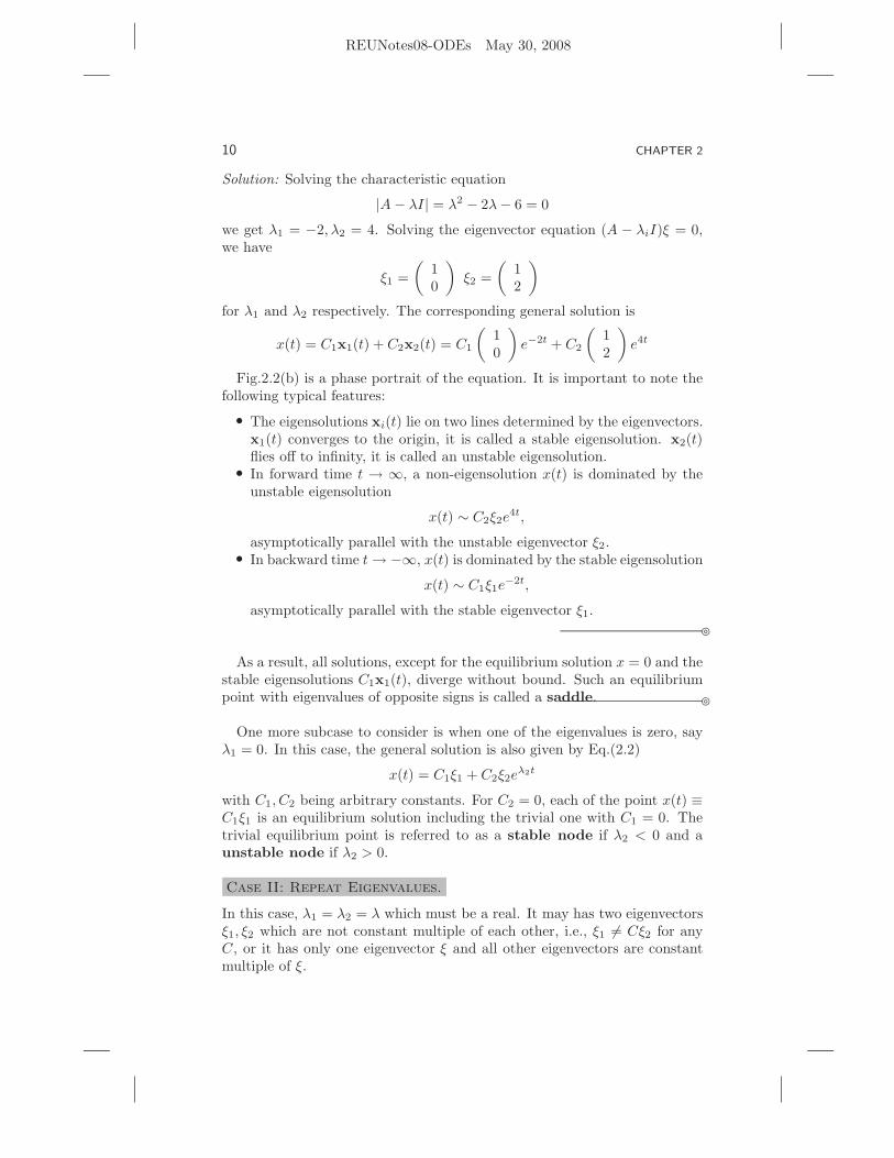
Fig.2.2(b) is a phase portrait of the equation. It is important to note thefollowing typical features:
• The eigensolutions xi(t) lie on two lines determined by the eigenvectors.x1(t) converges to the origin, it is called a stable eigensolution. x2(t)flies off to infinity, it is called an unstable eigensolution.
• In forward time t → ∞, a non-eigensolution x(t) is dominated by theunstable eigensolution
x(t) ∼ C2ξ2e4t,
asymptotically parallel with the unstable eigenvector ξ2.• In backward time t → −∞, x(t) is dominated by the stable eigensolution
x(t) ∼ C1ξ1e−2t,
asymptotically parallel with the stable eigenvector ξ1.da
As a result, all solutions, except for the equilibrium solution x = 0 and thestable eigensolutions C1x1(t), diverge without bound. Such an equilibriumpoint with eigenvalues of opposite signs is called a saddle. da
One more subcase to consider is when one of the eigenvalues is zero, sayλ1 = 0. In this case, the general solution is also given by Eq.(2.2)
x(t) = C1ξ1 + C2ξ2eλ2t
with C1, C2 being arbitrary constants. For C2 = 0, each of the point x(t) ≡C1ξ1 is an equilibrium solution including the trivial one with C1 = 0. Thetrivial equilibrium point is referred to as a stable node if λ2 < 0 and aunstable node if λ2 > 0.
Case II: Repeat Eigenvalues.
In this case, λ1 = λ2 = λ which must be a real. It may has two eigenvectorsξ1, ξ2 which are not constant multiple of each other, i.e., ξ1 6= Cξ2 for anyC, or it has only one eigenvector ξ and all other eigenvectors are constantmultiple of ξ.

REUNotes08-ODEs May 30, 2008
DIFFERENTIAL EQUATIONS 11
If it is the first scenario, it follows the same procedures as in the distinctreal eigenvalue case to obtain a general solution
x(t) = C1ξ1eλt + C2ξ2e
λt.
Generalized Eigensolutions. It is the second scenario that a refinedapproach is required. The method of trial solutions so far gives us only oneeigensolution x1(t) = ξeλt. It is not enough to form a general solution whichrequires two arbitrary constants. The goal is to find a second solution thatis not a constant multiple of x1(t).
To do this, we follow the same rationale that led to our first eigensolutionx1(t), which is obtained from the pool of candidate functions of the form ξeλt
whose derivatives are in the same pool. To find another solution outside thepool, we enlarge it but require still that its functions fit the characterizationthat their derivatives are also in the same pool. Here is such an enlargedpool: functions of this form
(η + tξ)eλt,
which are products of first degree polynomials and exponentials of a fixedparameter λ.
A few simple algebraic manipulations lead to the following
[(η + tξ)eλt]′ = (λη + ξ + tλξ)eλt = A(η + tξ)eλt = (Aη + tAξ)eλt
Cancelling out eλt and equating terms with t and terms without t (sincewe only need to find a solution as pragmatically as possible), we get thefollowing conditions on ξ, η, λ:
Aξ = λξAη = λη + ξ
⇐⇒ (A − λI)ξ = 0(A − λI)η = ξ
The first equation is the same eigenvalue-eigenvector relation obtained whenthe functional pool is the original smaller one, ξeλt. Solution η to the secondequation is called a generalized eigenvector. To find one, we first solvethe eigenvalue-eigenvector problem to get λ, ξ, and then solve the equation
(A − λI)η = ξ
for the generalized eigenvector, if indeed λ is a double eigenvalue, ξ is theonly eigenvector of λ and all others are constant multiple of ξ.
The resulting solution
(η + tξ)eλt
to the differential equation is called a generalized eigensolution.
Example 2.1.4 Find a general solution to the equations and sketch aphase portrait,
x′ =
[
0 4−1 −4
]
x

REUNotes08-ODEs May 30, 2008
12 CHAPTER 2
−1 −0.8 −0.6 −0.4 −0.2 0 0.2 0.4 0.6 0.8 1−1
−0.8
−0.6
−0.4
−0.2
0
0.2
0.4
0.6
0.8
1
−1 −0.5 0 0.5 1−1
−0.8
−0.6
−0.4
−0.2
0
0.2
0.4
0.6
0.8
1
(a) (b)
Figure 2.3 Phase portraits. (a) Example 4, (b) Example 5.
Solution: Solving the characteristic equation
|A − λI| = λ2 + 4λ + 4 = 0
we get λ1 = λ2 = λ = −2. Solve the eigenvector equation
(A − λI)ξ =
[
2 4−1 −2
](
u1
u2
)
=
(
00
)
We get
ξ =
(
−21
)
and the eigensolution x1(t) =
(
−21
)
e−2t.
To find a second solution, we solve the generalized eigenvector equation
(A − λI)η = ξ =⇒[
2 4−1 −2
] (
v1
v2
)
=
(
−21
)
.
It reduces to
v1 + 2v2 = −1.
Since we seek just one solution, assigning v2 = 0, v1 = −1 will do. Hence, ageneralized eigenvector and the corresponding generalized eigensolution are
η =
(
−10
)
and x2(t) = (η + tξ)eλt =
(
−1 − 2tt
)
e−2t respectively.
A general solution is thus given as
x(t) = C1ξe−2t + C2(η + tξ)e−2t =
(
−2C1 + C2(−1 − 2t)C1 + C2t
)
e−2t.
Fig.2.3(a) is a solution portrait of the equations in the phase plane ofx1, x2. It is important to note the following properties:

REUNotes08-ODEs May 30, 2008
DIFFERENTIAL EQUATIONS 13
• There is one radial line that contains solutions, the eigenvector linethrough the origin and the eigensolutions.
• Because of the negative eigenvalue, all solutions converge to the trivialsolution x = 0, i.e. limt→∞ x(t) = 0.
• In forward time as t → ∞, the term tξe−2t decays slower than the termswithout the multiple of t, it approximates and dominates the solution
x(t) ∼ C2ξteλ1t.
This explains why all solutions are asymptotically tangent to the eigen-vector radial line through the origin.
• In backward time as t → −∞, the term tξe−2t diverge faster than theterms without the multiple of t, it also approximates and dominates thesolution
x(t) ∼ C2ξteλ1t.
This explains why all solutions are asymptotically parallel to the eigen-vector line.
da
Remark. Because of the last two properties, a phase portrait for such a casecan be drawn without finding the generalized eigensolution. All needed arethe eigensolution and the vector field at one point. For example, at point(0, 1) the vector field is
A
(
10
)
=
[
0 4−1 −4
] (
01
)
=
(
4−4
)
,
pointing right-down. The only way to incorporate the asymptotic behaviorsand this piece of information on vector field is to have the phase portrait asshown.
Case III: Complex Eigenvalues.
Let λ1,2 = α ± iβ be the eigenvalues. In this case, we only need to use oneeigenvalue, say λ1 = α + iβ. Like all other cases, we proceed to find aneigenvector, which is usually a vector of complex entries. Let
ξ =
(
u1 + iv1
u2 + iv2
)
be an eigenvector with u1, u2, v1, v2 real numbers. We then separate it intoreal and imaginary parts in vector form as
ξ = u + iv where u =
(
u1
u2
)
and v =
(
v1
v2
)
.
That is both u and v are vectors of real entries. Following the deductionfor solutions, we know z(t) = (u + iv)eλt = (u + iv)e(α+iβ)t is a solution.However, it is complex valued, which is not what we eventually want. To findtwo real valued functions, we further separate z(t) into real and imaginary

REUNotes08-ODEs May 30, 2008
14 CHAPTER 2
parts of the form z(t) = x1(t) + ix2(t) with both x1(t),x2(t) real valuedfunctions. (See example below to learn how to carry out the separation.)Since z(t) is a solution, the following lines of reasoning show that bothx1(t),x2(t) are solutions as well.
x′
1(t) + ix′
2(t) = z′(t) = Az(t) = Ax1(t) + iAx2(t).
Equating real and imaginary parts, we have
x′
1(t) = Ax1(t) and x′
2(t) = Ax2(t).
Hence, both x1(t),x2(t) are real valued solutions, and the correspondinggeneral solution is given as usual
x(t) = C1x1(t) + C2x2(t).
Example 2.1.5 Find a general solution to the equations and sketch aphase portrait.
x′ =
[
−1 −24 −5
]
x
Solution: Solving the characteristic equation
|A − λI| = λ2 + 6λ + 13 = 0
gives λ1,2 = −3 ± i2. The eigenvector equation for λ1 is
(A − λ1I)ξ =
[
2 − i2 −24 −2 − i2
] (
z1
z2
)
=
(
00
)
which in components are
(2 − i2)z1 − 2z2 = 04z1 − (2 + i2)z2 = 0.
The two equations are redundant of each other, differing only by a constantmultiple (e.g., multiplying 1 + i and the first equation becomes the secondequation). A simple eigenvector is obtained by assigning z1 = 1 which givesz2 = 1 − i. Hence
ξ =
(
11 − i
)
and z(t) =
(
11 − i
)
e(−3+i2)t.
To separate z(t) into its real and imaginary parts, we use the Euler for-mula for complex exponential:
ea+ib = ea(cos b + i sin b).
Use it to get
e(−3+i2)t = e−3t+i2t = e−3t(cos(2t) + i sin(2t)).
Now using the complex multiplication rule
(a + ib)(c + id) = ac − bd + i(ad + bc),

REUNotes08-ODEs May 30, 2008
DIFFERENTIAL EQUATIONS 15
we separate the solution z(t) into its real and imaginary parts as follows:
z(t) =
(
11 − i
)
e−3t+i2t =
(
11 − i
)
e−3t(cos(2t) + i sin(2t))
=
(
e−3t cos(2t) + ie−3t sin(2t)e−3t(cos(2t) + sin(2t)) + ie−3t(sin(2t) − cos(2t))
)
= e−3t
(
cos(2t)cos(2t) + sin(2t)
)
+ ie−3t
(
sin(2t)sin(2t) − cos(2t)
)
:= x1(t) + ix2(t).
The corresponding general solution is
x(t) = C1x1(t) + C2x2(t)
= C1e−3t
(
cos(2t)cos(2t) + sin(2t)
)
+ C2e−3t
(
sin(2t)sin(2t) − cos(2t)
)
= e−3t
(
C1 cos(2t) + C2 sin(2t)(C1 − C2) cos(2t) + (C1 + C2) sin(2t)
)
Fig.2.3(b) is a solution portrait of the equations in the phase plane ofx1, x2. Important features are as follows:
• Because of the negative real part of the eigenvalue, all solutions convergeto the trivial solution x = 0, i.e. limt→∞ x(t) = 0.
• All solutions spiral around the equilibrium solution x = 0. The directionof spiral can be determined by the vector field at one point. For example,at point (1, 0), the vector field is
A
(
10
)
=
[
−1 −24 −5
] (
10
)
=
(
−14
)
.
It points left-up. Therefore the spiral is counterclockwise.da
Remark. Using the information of the real part of the complex eigenvaluesand the vector field at one point, one can qualitatively sketch the phaseportrait of the equation without solving it. For example, had the real partof the eigenvalues of the example above been positive and the vector field at(1, 0) been the same, solutions would spiral counterclockwise and away fromthe origin. da
Fig. 2.4 illustrates two more examples of the complex eigenvalue case.
Fig.2.4(a) is for the coefficient matrix A =
[
−0.1 −11 −0.1
]
for which the
real part, −0.1, of the eigenvalues is relatively small in magnitude, resultingin a looser spiral than that of Example 2.1.5 seen in Fig.2.3(b). Fig.2.4(b)
is for the coefficient matrix A =
[
0 1−1 0
]
for which the real part is zero,
giving rise to all closed cycles for its orbits. The trivial equilibrium point(0, 0) is referred to as a center. da

REUNotes08-ODEs May 30, 2008
16 CHAPTER 2
−1 −0.8 −0.6 −0.4 −0.2 0 0.2 0.4 0.6 0.8 1−1
−0.8
−0.6
−0.4
−0.2
0
0.2
0.4
0.6
0.8
1
−1 −0.8 −0.6 −0.4 −0.2 0 0.2 0.4 0.6 0.8 1−1
−0.8
−0.6
−0.4
−0.2
0
0.2
0.4
0.6
0.8
1
(a) (b)
Figure 2.4 Phase portraits with complex engensolutions: (a) A looser and clock-wise spiral; (b) A center.
The trivial equilibrium solution x = 0 to the linear equation x′ = Axis said to be asymptotically stable limt→+∞ x(t) = 0. It is not hard toshow that x = 0 is asymptotically stable for a linear system if and onlyif all eigenvalues of A have a negative real part. On the other hand, ifone eigenvalue has a positive real part, then the trivial equilibrium point isasymptotically unstable. For the case of Fig.2.4(b) for which the real partof the complex eigenvalues of A vanishes, the equilibrium point is stable butnot asymptotically stable.
Higher Dimensional Systems and the Routh-Hurwitz Criteria.
Theorem 2.1 (Routh-Hurwitz Criteria1) For the characteristic equa-
tion of an n×n coefficient matrix A of a linear system of equations x′ = Ax,
|λI − A| = λn + b1λn−1 + · · · + bn−1λ + bn = 0,
the eigenvalues λ all have negative real parts if
∆1 > 0, ∆2 > 0, . . . , ∆n > 0,
where
∆k =
∣
∣
∣
∣
∣
∣
∣
∣
∣
∣
∣
b1 1 0 0 0 0 . . . 0b3 b2 b1 1 0 0 . . . 0b5 b4 b3 b2 b1 1 . . . 0...
......
......
.... . .
...
b2k−1 b2k−2 b2k−3 b2k−4 b2k−5 b2k−6 . . . bk
∣
∣
∣
∣
∣
∣
∣
∣
∣
∣
∣
and bi = 0 if i ≥ n.
For the specific case of n = 2, the criteria reduces to
b1 = −tr(A) > 0 and b2 = det(A) > 0.

REUNotes08-ODEs May 30, 2008
DIFFERENTIAL EQUATIONS 17
For n = 3, it becomes
b1 = −tr(A) > 0, b2 =
3∑
k=1
det(Ak) > 0, b3 = − det(A) > 0, and b1b2 > b3,
where tr(A) is the trace of A (the sum of A’s diagonal entries), and Ak isthe matrix obtained from A by deleting the kth row and the kth column ofA.
Exercises 2.1
1. Find the solutions to the equations
(i) x′ = −2x, x(0) = 3
(ii) x′ =x
2, x(1) = 2
2. Find general solutions of the equations, determine the stability of theequilibrium solution x = 0, and sketch the phase portraits, which shouldinclude the eigensolutions of the equations if apply.
(i) x′ =
[
0 −12 −3
]
x
(ii) x′ =
[
1 21 0
]
x
(iii) x′ =
[
1 1−2 3
]
x
(Eigenvalues: (i) −1,−2. (ii) 2,−1. (iii) 2 ± i. )
3. Determine the stability of the equilibrium point x = 0 of the equations.
(i) x′ =
[
2 −11 0
]
x
(ii) x′ =
[
1 −36 −5
]
x

REUNotes08-ODEs May 30, 2008
18 CHAPTER 2
2.2 PHASE LINE AND BIFURCATION
Having solutions in formulas to differential equations are rare nor alwaysdesirable. In most cases we seek a qualitative understanding of the solutionstructure without displaying the solutions in formulas. The nature of suchmethods are inevitably conceptual and geometrical.
Here we introduce a qualitative method for the simplest class of nonlineardifferential equations: the autonomous equations of one dimension:
x′ = f(x).
A solution x(t) is simply a function of the time variable t. They are remark-ably simple for equations. The solution x(t) can behave only in one of thefollowing three ways:
• x(t) remains constant for all t, which is called an equilibrium solution,or equilibrium point.
• x(t) monotone increases either without bound or approaches an equilib-rium point.
• x(t) monotone decreases either without bound or approaches an equi-librium point.
These properties are captured by the graphs below.
On the left is the graph of the right hand of the equation. Its x-intercepts,a, b, c, captures all the equilibrium points. These points divide the phasespace, i.e., the x-axis, into intervals in each of which the rate of changefunction f can take on one sign, positive or negative, since the only placeswhere it can possibly change signs are the equilibrium points at the endpoints of the intervals. This implies that starting at any point inside aninterval with positive f , the solution increases in time and stays in the sameinterval. Similarly, a solution decreases and stays in an interval of negativesign of f if it starts in the same interval. The arrows designate the directionsof the orbital monotonicity.
On the right is a qualitative depiction of some typical solutions as func-tions of the independent variable t. Equilibrium solutions stay as horizontallines. Others either converge to or away from equilibrium solutions. It isuseful to note that this solution portrait does not offer substantially addi-tional information than the features already annotated on the x-axis in the

REUNotes08-ODEs May 30, 2008
DIFFERENTIAL EQUATIONS 19
Existence and Uniqueness of Solutions. An important theoretical question is ifan initial value problem (
x′ = f(t, x)
x(t0) = x0
has a solution and if it has a unique solution. The answer depends on the function f .If f is continuously differentiable with respect to both t and x in a neighborhood ofthe initial point (t0, x0), then it has a unique solution. In fact, the same conclusionholds for somewhat weaker conditions, such as f is Lyapunov continuous. (A typ-ical example of Lyapunov continuity is the function of absolute value f(t, x) = |x|.Piecewise linear functions is another.) Hence, the existence and uniqueness questionis rarely an issue for differential equation models from sciences and engineering fields.
One immediate and importance consequence to the uniqueness of solutions to initialvalue problems is that solutions having different initial conditions never intersect atany moment in time. For example, the solution plot of two different solutions in thetx-space must not intersect.
A special consequence is worth noticing for autonomousequation x′ = f(x) in any dimensions. It is based on theproperty specific for such equations that if x(t) is a solu-tion, so is any time translation x(t + θ). (Just differentiateand plug it into the equation to check.) The projection ofa solution (t, x(t)) to the phase space x is the parameter-ized curve x(t), which is called an orbit. The uniquenessproperty of solutions to initial value problems implies thatan orbit cannot cross itself nor another orbit. For exam-ples, the top two figures on the right are possible orbits butthe bottom two are not. (There are five orbits depicted inthe upper-left figure, including the open dot representingan equilibrium orbit.)
One important exception is Newton’s law of gravity which introduces singularities toequations governing celestial bodies. As a result solutions may not be unique comingout the singularities, and celestial bodies do smash onto each others from time totime.
left figure. In fact, the diagram has captured all important qualitative infor-mation of the equation. For this reason we refer to such a plot as the phaseline, which is extracted and depicted alone as below.
You may have notices that solutions do not behave the same near allequilibrium points. We have the following classifications:
• An equilibrium point is a sink if all solutions nearby converge to it.• An equilibrium point is a source if all solutions nearby diverge from it.• An equilibrium point is a node if some solutions converge to it and
some others diverge from it.
In the example depicted above, a is a sink, b is a source, and c is node.

REUNotes08-ODEs May 30, 2008
20 CHAPTER 2
We also say that a sink is asymptotically stable or a sink attracts allsolutions nearby, and a source is asymptotically unstable or it repels allsolutions nearby. A node is simply unstable.
Example 2.2.1 Sketch the phase lines of equations and classify the equi-librium points.
(a) x′ = x2 − x (b) x′ = (1 − x2)(x − 2)2
x′
x
x′ = x2 − x
0 1+ _+
(a)
x
x′x′ = (1−x2)(x−2)2
−1 1 20
_ + _ _
(b)
Solution: (a) First we plot the right hand of the equation as shown. Itintersects the x-axis at x = 0, 1, which are the equilibrium points. Thesigns of f(x) = x2 − x in intervals partitioned by the equilibrium pointsare determined by the relative position of the graph to the x-axis, + if it isabove the x-axis, − if it is below. The arrows are placed according to thesigns, right arrow for + and left arrow for −. These intervals with assignedarrows are called orbits, which are the projections to the phase space xof the solutions (t, x(t)) from the tx-plane. We conclude from the phase lineplot that equilibrium point x = 0 is a sink and x = 1 is a source.
(b) Following the same steps, the solution is given by the graph. Forstabilities of equilibrium points, x = −1 is a sink, x = 1 is a source, andx = 2 is a node.
da
Phase Lines with Parameter and Bifurcations. We consider nextequations that depends on one parameter,
x′ = f(x, λ),
where t, x are the variables and λ is the parameter. For each fixed λ value,the qualitative dynamics of the equation is captured by its phase line. Thestructure of the phase line may change for a different λ value. To see suchchanges, we may plot the phase lines one λ value a time. But this is cum-bersome and inefficient — it is not possible to draw phase lines for all λvalues.
There is a more effective way. It is based on a lesson learned from thephase line plot. That is, the equilibrium points of the equation together withthe sign of the right hand of the equation determine the phase line structure.The phase line method with parameter is illustrated below.
The steps are summarized as follows.

REUNotes08-ODEs May 30, 2008
DIFFERENTIAL EQUATIONS 21
1. In the xλ-plane, plot the level curve f(x, λ) = 0, called the equilib-rium branch. A point, (x, λ), on the curve gives an equilibrium pointx of the equation for the given parameter λ.
2. The equilibrium branch or branches divides the region of interest intosubregions, in each of which f(x, λ) does not vanish and therefore ithas a fixed sign.
3. To sketch the phase line for a fixed value λ, just draw the horizontalline through λ. Any intersection of the line with the equilibrium brandf(x, λ) = 0 is an equilibrium point for the equation for that λ value.The line is partitioned into intervals by the equilibrium points, fallinginto f > 0 and f < 0 regions. The orbital structure is then drawn onthe line as you would for a phase line.
4. Use solid curves for the parts of the equilibrium branch whose equilib-rium points are stable and dash curves for the ones whose equilibriumpoints are unstable. They are referred to as the stable equilibriumbranches and unstable equilibrium branches, respectively.
In the hypothetical illustration above, we see that there are typical parametervalues for which the qualitative structure of phase lines do not change if onechange the parameter near by, such as the ones not going through the criticalpoints of the equilibrium branch. Yet there are a few atypical parametervalues that stand out, such as the ones going through the critical points. Aslight increase or decrease from these special values give rise to qualitativelydifferent phase lines, especially in the number of equilibrium points and theirstabilities. We refer to such a phenomenon as bifurcation. In particular,we call a point, (x, λ), a bifurcation point, if f(x, λ) = 0 and if the phaseline changes qualitatively near the equilibrium point x when λ varies slightlyfrom λ.
We will introduce the types of bifurcation to be encountered in this chapterthrough examples. These are saddle-node bifurcation, transcritical bifurca-
tion, and Hopf bifurcation. Other types that will not be used are introducedthrough exercises. The Hopf bifurcation is for 2-dimensional systems and itwill be introduced in a later section.
Saddle-Node Bifurcation.
Example 2.2.2 Consider the logistic model with a constant harvest rateH ,
dP
dt= rP
(
1 − P
K
)
− H (2.3)
where r is the maximum per-capita growth rate, K is the carrying capacity,and H is the constant harvest rate. Sketch the phase lines using H as theparameter.Solution: The equilibrium branch is defined by rP (1 − P
K ) − H = 0. By
chance, it can be solved as H = rP (1 − PK ) in the PH-plane. The branch
divides the plane into two parts: P ′ > 0 below the branch and P ′ < 0

REUNotes08-ODEs May 30, 2008
22 CHAPTER 2
Logistic Model. Let P (t) be a population measure of a species at time t. The timet can be in second, or day, or year, etc, and population P can be in a nonnegative
number for the total biomass, or density. The derivativedP (t)
dtis the growth rate,
and1
P (t)
dP (t)
dt
defines the per-capita growth rate. P ′(t) > 0, the population increases. P ′(t) < 0,it decreases. P ′(t) ≡ 0 for all t, it stays at an equilibrium, or steady state, P (t) ≡a constant.
The logistic model for population growth is to assume that the per-capita growth rate
is proportional a dimensionless factor 1 −P (t)
K, that is
1
P (t)
dP (t)
dt= r
�1 −
P (t)
K
�with r, K been nonnegative constants. Since P ≥ 0, r is the maximal per-capita rate,referred to as the intrinsic rate. For P < K, the per-capita rate P ′/P is positive,and the population increases. For P > K, P ′/P < 0, and the population decreases.For this reason, K is called the carrying capacity.
P′
P0 K
+ __
The model is usually presented in the following standard equational form
dP
dt= rP
�1 −
P
K
�By a phase line analysis, we find that P = 0, K are the only equilibrium points, forwhich P = 0 is a source and P = K is a sink. Thus, for any nonvanishing initialpopulation P0, the solution through P0 at t = 0 converges to K, i.e., the populationeventually stabilizes at its carrying capacity K.
above the branch. The branch has a maximum point in H . It is found byelementary calculus to be
(P , H) =
(
K
2,rK
4
)
.
The parameterized phase lines are asshown. Notice the qualitative differencesfor harvesting rate H above and below H.H is a bifurcation value and (P , H) is abifurcation point by definition.
da
More precisely, the bifurcation point (P , H) of this example is a prototyp-ical case of a saddle-node bifurcation. It is characterized by the following.
Definition 2.2 An equilibrium point (x, λ) of
x′ = f(x, λ)
is a saddle-node bifurcation point if it satisfies the following conditions:

REUNotes08-ODEs May 30, 2008
DIFFERENTIAL EQUATIONS 23
• For λ from one side of λ, the equation has two equilibrium points, one
stable and one unstable. Both equilibrium points emerge at x as λ con-
verges to λ• For λ from the other side of λ, the equation does not have an equilibrium
point near x. That is as λ crosses λ into this region, the two equilibrium
points emerge at x and then disappear.
The mathematical results of the example above have the following biolog-ical interpretations.
• For H < H , the right equilibrium point is the continuation of the car-rying capacity, and it is stable. The equilibrium state decreases whenthe harvest rate H increases. Thus this branch right of the bifurcationstate P is called the harvest mediated carrying capacity.
• For H < H , the left equilibrium state is the continuation of the non-existence state P = 0, and it is unstable. In contrast, it increases whenH increases. If the population starts below the left equilibrium, it willreach the extinction state P = 0 in a finite time. If it starts abovethe equilibrium, it converges to and stabilizes at the harvest inducedcarrying capacity. For this reason, the equilibrium branch left of P iscalled the harvest mediated survival threshold.
• Because the threshold branch increases and the capacity branch de-creases as H increases, the two branches head to each other. In thiscase they co... at the bifurcation point P , which is also referred to asa crash fold point. For the harvest rate greater than the critical valueH , the population crashes down and eventually dies out, regardless itsinitial population.
Transcritical Bifurcation.
Example 2.2.3 Consider the logistic model with a constant per-capita
harvest rate,
dP
dt= rP
(
1 − P
K
)
− hP (2.4)
where as before r is the maximum per-capita growth rate, K is the carryingcapacity, and h is the constant per-capita harvest rate. Sketch the phaselines using h as the parameter.Solution: The equilibrium branch is defined by rP (1− P
K )−hP = 0. Unlikethe constant harvest case, it is solved into two branches:
P = 0 and r
(
1 − P
K
)
− h = 0.
The latter defines a line, having h = r as the h-intercept and P = K as theP -intercept.

REUNotes08-ODEs May 30, 2008
24 CHAPTER 2
By inspection, we see that (P , h) =(0, r) is a bifurcation point. Specifically,the threshold branch P = 0 changes itsstability from unstable to stable as h in-creases through r. And the capacitybranch through (K, 0) changes its stabil-ity from stable to unstable.
da
The bifurcation point (P , h) = (0, r) of this example is a prototypical caseof a transcritical bifurcation. It is characterized by the following.
Definition 2.3 An equilibrium point (x, λ) of
x′ = f(x, λ)
is a transcritical bifurcation point if it satisfies the following conditions:
• There are two branches of equilibrium points intersect at (x, λ) at a
nonvanishing angle.• The equilibrium point on any branch of the two exchanges stability as
the parameter λ passes through λ.
In the context of population dynamics, the transcritical bifurcation point(0, r) of the example above is called the capacity transcritical point. Insome cases where the transcritical bifurcation takes place on the survivalthreshold branch, the point is called the threshold transcritical pointinstead.
Exercises 2.2
1. Sketch the phase lines of the equations; determine the stabilities of theequilibrium points; and sketch the solution portraits in the tx-plane aswell.
(i) x′ = −x3 + 2x2 − x
(ii) x′ = −x3 + 2x2 − x + 0.5
(iii) x′ = 2 sin(πx)
2. Find all equilibrium points, and determine their stabilities by the deriva-tive test. Verify your answer schematically by sketch the phase lines.
(i) x′ = x3 − x2 − 2x
(ii) x′ = x − x2 − 0.3x
0.25 + xfor x ≥ 0.

REUNotes08-ODEs May 30, 2008
DIFFERENTIAL EQUATIONS 25
3. Sketch the bifurcation diagram of this one-parameter family of differentialequations
x′ = fa(x) = ax − x3.
The type of bifurcation points this example represent is called Pitch-forkBifurcation.
Problem 4
4. Consider the RC-circuit shown with an ‘N ’ nonlinear IV characteristicsI = F (V ) = V 3 − 2V 2 + V . It is model by this one-parameter family ofequations
CdVC
dt= −F (E + VC) − Iin
with the forcing current Iin being the parameter. Sketch the bifurcationdiagram of the equations, and identify the type of bifurcation.
5. Consider the predator-prey model
x′ = x(1 − x) − x
β + xy
for which the predator population density y is considered as a parameter.For a fixed vale
0 < β < 1
sketch the bifurcation diagram in the first quadrant x ≥ 0, y ≥ 0 with ybeing a parameter.

REUNotes08-ODEs May 30, 2008
26 CHAPTER 2
2.3 PHASE PLANE METHOD
We now extend the phase line method to autonomous systems of two equa-tions
{
x′ = f(x, y)
y′ = g(x, y)(2.5)
where f, g are nice functions which guarantee the uniqueness of solutions toinitial value problems.
In the (x, y) phase space, a solution gives rise to an orbit {(x(t), y(t))} asa curve parameterized by the time variable t. At each point of the orbit, itmoves in the direction and speed given by the velocity vector (x′(t), y′(t)),which is prescribed by the vector field (f(x(t), y(t)), g(x(t), y(t))). That is,an orbit is not just any curve in the phase space. It must follow the vectorfield (f(x, y), g(x, y)) at every point (x, y) in the space. See illustration.
The description above gives rise to the following approximation of orbits.We generate a mesh grid in x, y with a user defined mesh size. At eachgrid point (xi, yj), we plot the vector field (f(xi, yj), g(xi, yj)). Then anorbit starting at any point inside the mesh can be sketched by following thevector field as closely as possible.
Though the method above is suitable for computers, it does not make agood use of human intuitions. This is where the phase plane method enters.It gives an insightful and systematic way to organize the vector field. Insome cases it gives a rather comprehensive, qualitative understanding onthe orbital structure of the equations. In the cases it fails to be complete, itnevertheless gives a good, first order approximation to the structure.
The Method
Like the phase line method, the phase plane method again makes use ofequilibrium points to organize the vector field. Particularly indispensableare the curves defined by f(x, y) = 0 and g(x, y) = 0. If one thinks y as aparameter, the former f(x, y) = 0 would define the equilibrium branch forthe x-equation. Symmetrically, if one thinks x as a parameter, the latterg(x, y) = 0 would define the equilibrium branch for the y-equation. Forthese reasons, we call the curve f(x, y) = 0 the x-nullcline and g(x, y) = 0the y-nullcline.
Here is a brief description for the procedures.
1. In the (x, y) phase space, sketch the x-nullcline f(x, y) = 0. It dividesthe space into regions of f > 0 and f < 0. Use the one-point testingtechnique to label these regions.
2. Do the same for the y-equation: sketch the y-nullcline g(x, y) = 0 andidentify the regions with g > 0 and g < 0.
3. On each segment of the x-nullcline partitioned out by the equilibriumpoints, place a vertical vector filed (x′, y′) = (0, g). The vector points

REUNotes08-ODEs May 30, 2008
DIFFERENTIAL EQUATIONS 27
up if the segment lies in a y′ = g > 0 region, and points down ifotherwise.
4. Do the same for the y-nullcline, in reverse. That is one each segment ofthe y-nullcline, place a horizontal vector filed (x′, y′) = (f, 0), pointingright if it lies in a x′ = f > 0 region or left if it lies in a f < 0 region.
5. In each region bounded by x-nullcline and y-nullcline, the vector field(f, g) never vanish in either component. Place a vector inside the regionaccording to the following convention
sign(x′, y′): [+,+] [+,−] [−,+] [−,−]
vector field (x′, y′): ր ց տ ւ
description: right-up right-down left-up left-down
6. Sketch any special as well a few typical orbits following the directionsof the vector field in the regions bounded by the nullclines. In theillustration below, for example, orbit 1 coming out the equilibriumpoint in the [+, +] region is such a special orbit, called separatrix.It moves right-up in the region. Orbit 2 is another. Orbits 3 and 4are typical ones. Notice that orbit 3 must be drawn to move left-upin the [−, +] region, cross the x-nullcline vertically, turn around in thex-component and move right-up in the [+, +] region. In contrast, whenorbit 4 crosses the y-nullcline, it must do so horizontally.
As one can see in the illustration above, one can fill other special andtypical orbits in the [+,−] and [−,−] regions to complete the steps of themethod. Also, in this hypothetical case, the orbital structure near the equi-librium point shown is completely understood — it has the structure of asaddle point.
A word of caution for beginners. Equilibrium points lie always on null-clines, but only in rare situations a nullcline becomes a solution to the dif-ferential equations.
Phase Portrait of 2-D Linear Systems.
To illustrate the method, we first use it on a linear system to show howthe phase portraits of such systems can be completely understood especially
REUNotes08-ODEs May 30, 2008
28 CHAPTER 2
when combining with the information of their eigensolutions.
Example 2.3.1 Recall the linear system of equations (2.1.3) from Sec.2.1 together with their linearly independent eigensolutions:
x′ =
[
−2 30 4
]
x, x1(t) =
(
10
)
e−2t, x2(t) =
(
12
)
e4t.
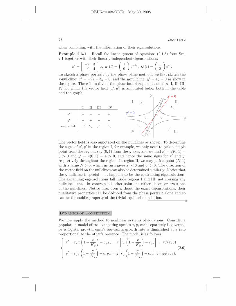
To sketch a phase portrait by the phase plane method, we first sketch thex-nullcline: x′ = −2x + 3y = 0, and the y-nullcline: y′ = 4y = 0 as show inthe figure. These lines divide the plane into 4 regions labelled as I, II, III,IV for which the vector field (x′, y′) is annotated below both in the tableand the graph.
I II III IV
x′ + − − +
y′ + + − −
vector field ր տ ւ ց
The vector field is also annotated on the nullclines as shown. To determinethe signs of x′, y′ in the region I, for example, we only need to pick a simplepoint from the region, say (0, 1) from the y-axis, and we find x′ = f(0, 1) =3 > 0 and y′ = g(0, 1) = 4 > 0, and hence the same signs for x′ and y′
respectively throughout the region. In region II, we may pick a point (N, 1)with a large N > 0, which in turn gives x′ < 0 and y′ > 0. The direction ofthe vector field on the nullclines can also be determined similarly. Notice thatthe y-nullcline is special — it happens to be the contracting eigensolutions.The expanding eigensolutions fall inside regions I and III, not crossing anynullcline lines. In contrast all other solutions either lie on or cross oneof the nullclines. Notice also, even without the exact eigensolutions, theirqualitative properties can be deduced from the phase portrait alone and socan be the saddle property of the trivial equilibrium solution.
da
Dynamics of Competition.
We now apply the method to nonlinear systems of equations. Consider apopulation model of two competing species x, y, each separately is governedby a logistic growth, each’s per-capita growth rate is diminished at a rateproportional to the other’s presence. The model is as follows
x′ = rxx
(
1 − x
Kx
)
− cyxy = x
[
rx
(
1 − x
Kx
)
− cyy
]
:= xf(x, y)
y′ = ryy
(
1 − y
Ky
)
− cxyx = y
[
ry
(
1 − y
Ky
)
− cxx
]
:= yg(x, y).
(2.6)

REUNotes08-ODEs May 30, 2008
DIFFERENTIAL EQUATIONS 29
Here ri, Ki are the intrinsic rates and carrying capacities, and cj > 0 are theper-capita competition coefficient of species j against species i.
Species x is said to be competitive if its per-capita growth rate is positiveat the y-capacity point (0, Ky), that is
1
x
dx
dt
∣
∣
∣
(0,Ky)= f(0, Ky) = rx − cyKy > 0 ⇐⇒ Ky <
rx
cy.
Notice that according to this characterization, species x is competitive ifspecies y’s per-capita adversary impact coefficient cy is relatively small.Similarly, y is competitive if it can grow per-capita at the x-capacity point(Kx, 0) so that
Kx <ry
cx.
Example 2.3.2 (Competitive Coexistence.) Use the phase plane methodto analysis the dynamics of the competition model Eq.(2.6) when bothspecies are competitive, i.e.,
Kx < ry/cx and Ky < rx/cy.
Solution: We begin by sketch the x-nullcline: xf(x, y) = x[rx(1 − x/Kx) −cyy] = 0 which are separated into two branches
x = 0 and rx(1 − x/Kx) − cyy = 0.
The latter is the y-competition mediated x-carrying capacity: along whichx decreases as y increases, having the x-intercept at the x-carrying capacity(Kx, 0), and the y-intercept at the x-capacity transcritical point (0, rx/cy).See the illustration.
Similarly, the y-nullcline yg(x, y) = y[ry(1 − y/Ky) − cxx] = 0 has twobranches
y = 0 and ry(1 − y/Ky) − cxx = 0,
with the latter being the x-competition mediated y-carrying capacity: alongwhich y decreases as x increases, having the y-intercept at the y-carryingcapacity (0, Ky), and the x-intercept at the y-capacity transcritical point

REUNotes08-ODEs May 30, 2008
30 CHAPTER 2
(ry/cc, 0). Because of the dual competitive assumption, the x-capacity tran-scritical rx/cy is greater than the y-capacity Ky on the y-axis and the y-capacity transcritical ry/cx is greater than the x-capacity Kx on the x-axisas shown.
Next, we label the subregions in the first quadrant that are bounded by thenullclines as I, II, III, IV. The signs of f, g in these regions are as shown below.The signs are determined by one-point test technique. For example, in region
I II III IV
x′ + − − +
y′ + + − −
vector field ր տ ւ ց
I, the sign of x′ can be determined by evaluating x′ = xf(x, y) at anypoint in the region. Taking (Kx/2, 0) for convenience, we find x′|(Kx/2,0) =(Kx/2)f(Kx/2, 0) > 0 and hence a ‘+’ sign in the table.
Having determined the directions of the vector field (x′, y′), a representa-tive vector field is placed in each of the region.
One the nullclines, the vector field is either horizontal or vertical. Forexample, on the part of the y-nullcline which forms the common boundaryof region I and region IV , x′ is positive. Hence, it is given a right arrow.
Last, we are ready to sketch special and typical orbits. First, equi-librium orbits are simply the intersections of the x-nullcline and the y-nullcline. There are 4 of them, the trivial mutual extinct state (0, 0), thecompetition-free individual capacity states (Kx, 0), (0, Ky), referred to as thex-equilibrium and the y-equilibrium respectively, and the coexistent statereferred to as the xy-equilibrium. The xy-equilibrium point can be solvedexplicitly from f(x, y) = 0, g(x, y) = 0 if needed.
There are at least four special, non-equilibrium orbits, one in each regionI, II, III, IV, connecting equilibrium orbits without crossing the nullclines.
Last, sketch a few typical solutions to complete the phase portrait. Forexample, starting at any point in region III, below the special orbit converg-ing to E, the orbit must develop left and down, cross the y-capacity nullclinehorizontally, turn upward but still move left, remain in region II thereafterand tend to E. E is asymptotically stable.
We can now conclude that starting at nonvanishing populations for bothspecies x0 > 0, y0 > 0, the orbit converges to the equilibrium point E. Thebiological significance of this result is that mutually competitive species cancoexist at an equilibrium state in a long run.
da
We have used two figures in the example above to highlight the steps. Youcan certainly plot the orbital structure from the right figure onto the left oneif it does not become too cluttered.

REUNotes08-ODEs May 30, 2008
DIFFERENTIAL EQUATIONS 31
Again like the case of phase lines, the phaseportrait of a system of equations captures allessential geometric properties of the solutionsto the system. For example, one can qualita-tively construct the time series of a solutionfrom its orbit in the phase plane. The timesseries on the right are reconstructed for Or-bit 1 from the phase portrait of the exampleabove. We note that the vertical dash lineindicates the time at which the orbit crossesthe x-nullcline before its converging to the co-existing equilibrium point.
Example 2.3.3 (Competitive Tug of War.) Use the phase plane methodto analysis the dynamics of the competition model Eq.(2.6) when bothspecies are not competitive, i.e.,
Kx > ry/cx and Ky > rx/cy.
Solution: We follow the same steps and analysis as in the previous example.The critical difference in result is that the the x-capacity branch and the y-capacity branch switch their relative position with each other, in particularthe competition free capacities Ki switch position with the capacity trans-critical point rj/ci on the axis i. As a result, the vector field are drasticallydifferent in subregion II and IV as shown in the table below. By making
I II III IV
x′ + + − −
y′ + − − +
vector field ր ց ւ տ
appropriate changes to the previous plot, a phase portrait is shown below.Again one can use just one plot by including the orbits in the left figure ifit is not too cluttered.

REUNotes08-ODEs May 30, 2008
32 CHAPTER 2
Orbit 1 and orbit 2 are separatrixes. They divide the first quadrantinto two parts. The region above the separatrixes is the non-competitiveregion for x, in which all orbits converge to the y-capacity state (0, Ky)with x driven to extinction. The region below the separatrixes is the non-competitive region for y, in which all orbits converge to the x-capacity state(Kx, 0) with y driven to extinction. In other words, the outcome depends onthe initial state of the population. Initial states on the separatrixes or theequilibrium state E cannot persist. Any small perturbation will throw thestates into one of the non-competitive regions, driving off one competitor.There is no coexisting state.
da
The remaining case with one species competitive and the other not is leftas an exercise, which leads to the phenomenon of competitive exclusion.
Exercises 2.3
1. The nullclines and some information about the vector field for a systemare given in each of the diagram. Use the phase plane method to sketcha phase portrait of each system.
(a) (b)
(Remark: Problem (b) would expose a weakness of the method.)
2. Consider again Problem 2 of Exercise 2.1. Refine the phase portraits ofthe equations by incorporating the phase plane method.
(i) x′ =
[
0 −12 −3
]
x
(ii) x′ =
[
1 21 0
]
x
(iii) x′ =
[
1 1−2 3
]
x
3. Consider the population model of two competing species Eq.(2.6). Usethe phase plane method to sketch a phase portraits for the case in whichone species is competitive and the other is not. The dynamics outcomeof such a case is referred to as competitive exclusion.

REUNotes08-ODEs May 30, 2008
DIFFERENTIAL EQUATIONS 33
4. Consider the population model of two cooperative species x, y:
x′ = rxx
(
1 − x
Kx
)
+ byxy
y′ = ryy
(
1 − y
Ky
)
+ bxyx
where all parameters ri, bj are positive.
(a) Show that it has an equilibrium point E = (Ex, Ey) with positivecomponents Ex > 0, Ey > 0 under the following condition
bxby <rxry
KxKy
(b) Use the phase plane method to sketch a phase portrait of this case.
REUNotes08-ODEs May 30, 2008
34 CHAPTER 2
2.4 PHASE PLANE WITH FAST AND SLOW TIME SCALES
The dynamics of a system of equations is determined by its vector field. Thephase plane method takes into account the direction of the vector field butignores so far its magnitude. This works well for some cases such the onesconsidered in the previous section. In this section, however, we considersystems for which the magnitude of their vector fields is too obvious toignore. Such are systems having different time scales.
Consider systems of the following form{
εx′ = f(x, y)
y′ = g(x, y)(2.7)
where 0 < ε ≪ 1 is ‘very’ small parameter as signified by the notation ‘≪ 1’.Looking at it from the point view of vector field, it is more convenient towrite it as
x′ =f(x, y)
εy′ = g(x, y)
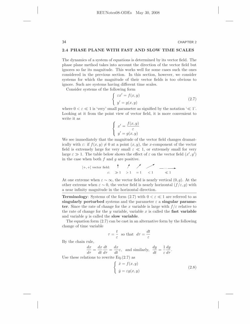
We see immediately that the magnitude of the vector field changes dramat-ically with ε: if f(x, y) 6= 0 at a point (x, y), the x-component of the vectorfield is extremely large for very small ε ≪ 1, or extremely small for verylarge ε ≫ 1. The table below shows the effect of ε on the vector field (x′, y′)in the case when both f and g are positive.
[+,+] vector field: 6 �� �� ��*... -
ε: ≫ 1 > 1 = 1 < 1 ≪ 1
At one extreme when ε ∼ ∞, the vector field is nearly vertical (0, g). At theother extreme when ε ∼ 0, the vector field is nearly horizontal (f/ε, g) witha near infinity magnitude in the horizontal direction.
Terminology: Systems of the form (2.7) with 0 < ε ≪ 1 are referred to assingularly perturbed systems and the parameter ε a singular parame-ter. Since the rate of change for the x variable is large with f/ε relative tothe rate of change for the y variable, variable x is called the fast variableand variable y is called the slow variable.
The equation form (2.7) can be cast in an alternative form by the followingchange of time variable
τ =t
εso that dτ =
dt
εBy the chain rule,
dx
dτ=
dx
dt
dt
dτ=
dx
dtε, and similarly,
dy
dt=
1
ε
dy
dτ.
Use these relations to rewrite Eq.(2.7) as{
x = f(x, y)
y = εg(x, y)(2.8)

REUNotes08-ODEs May 30, 2008
DIFFERENTIAL EQUATIONS 35
where z =dz
dτ.
Because of the conversion relation τ = t/ε, t is called the fast time andτ is called the slow time. For example, if the unit of t is in year, andε = 10−3, then 1 year in the t time scale equals 1000 years in the τ timescale. Correspondingly, the original form Eq.(2.7) is the singularly perturbedsystem in the fast time scale and the equivalent form Eq.(2.8) is the systemin the slow time scale.
Time Scale Method.
The theory of singular perturbation is about how dynamics of singularlyperturbed systems change with their singular parameters. Here we introducethe most elementary geometric method of the theory. It incorporates thethe diverging magnitude of a singularly perturbed vector field into the phaseplane method. Thus, we may call it phase plane method with timescales or simply the time scale method. Essential to the method are twotypes of orbits at the singular limit ε = 0. We begin with the simpler kind.
Fast Orbits.
This orbit type is associated with the slow time scale system (2.8) at thesingular limit ε = 0:
{
x = f(x, y)
y = 0.(2.9)
It is called the fast subsystem of the perturbed systems (2.7,2.8). This mayfirst appear paradoxical and confusing. However, upon a further reflection,it makes a perfect sense — a fast moving object is best analyzed in a slowmotion time scale.
The key realization that drives the analysis for this subsystem is that be-cause x moves so fast, variable y appears frozen in time. The equation y = 0says it all: y stays at its initial state wherever it starts, and therefore it canbe thought as a parameter one value a time. Hence, the orbital structure ofthe subsystem is completely determined by the phase line method with pa-rameter from Sec.2.2. For illustration purposes, let the x-equilibrium branch(more accurately the x-nullcline for the full system), f(x, y) = 0 be as inFig.2.5(a) together with phase lines parameterized by the slow variable y.The phase line x-orbits are called the fast orbits.

REUNotes08-ODEs May 30, 2008
36 CHAPTER 2
Algebraic-to-Differential Reduction Method for Slow Solutions. One wayto find a solution (x(t), y(t)) with an initial point (x(0), y(0)) = (x0, y0) to the slowsubsystem (2.10) is to follow the steps below.
1. Verify that point (x0, y0) is on the x-nullcline, satisfying f(x0, y0) = 0.2. Check if variable x can be uniquely solved as a function of variable y, i.e. x =
x(y), from the algebraic equation f(x, y) = 0 in a small open interval containingy0 satisfying x(y0) = x0.
3. If both conditions above are satisfied, then solve the reduced initial value problem(y′ = g(x(y), y)
y(0) = y0
4. If y(t) is a solution, then a solution to the slow subsystem is found by backwardsubstitution as (x(y(t)), y(t)).
Whether or not this analytical method works critically depends on the second con-dition above. By definition, a point (x∗, y∗) is called a turning point if it satisfiesf(x∗, y∗) = 0 but x cannot be uniquely solved from f(x, y) = 0 as a function of y.Hence, the solution procedure above fails at a turning point. As a result the slowsubsystem may or may not have a solution, or if it does, the solution may not be aunique solution.
Turning points are not new. We have encountered them in a different disguise. Infact, we have the following duality.
Turning Points are Bifurcation Points:
A point (x∗, y∗) is a turning point of the slow subsystem (2.10) if andonly if it is a bifurcation point of the fast subsystem (2.9).
Slow Orbits.
This orbit type is associated with the fast time scale system (2.7) at thesingular limit ε = 0:
{
0 = f(x, y)
y′ = g(x, y)(2.10)
It is called the slow subsystem of the perturbed systems (2.7,2.8). Again,similarly to the reason of analyzing the fast dynamics at the slow time scale,it is best to analyze slowly moving objects at a fast time scale.
The key realization that drives the analysis for this subsystem is that itsorbits must lie on the x-nullcline, f(x, y) = 0, and the dynamics is drivenprimarily by the y-equation. Since the equation is only one-dimensionalon the x-nullcline curves, the phase line method can be adapted onto therestricted curves. As a result the dynamical structure is rather simple.da
Slow Solution Structures. The orbits of the slow subsystem can onlybehave in one of the following three ways:
• Stay at an equilibrium state.• Monotone increase or decrease toward an equilibrium state.

REUNotes08-ODEs May 30, 2008
DIFFERENTIAL EQUATIONS 37
(a) (b)
(c) (d)
Figure 2.5 Time Scale Method
• Monotone increase or decrease toward a turning point of the systemthat defines a boundary point of the x-nullcline branch to which theslow subsystem is restricted.
da
In other words, the structure is completely determined by equilibrium pointsand turning points. It is this geometric approach that we will use predomi-nantly throughout.
The phase line method for the slow subsystem is illustrated as in Fig.2.5(b)which is the continuation of the hypothetical case of Fig.2.5(a). The directedcurves on the x-nullcline are the orbits of the slow subsystem. They arecalled the slow orbits. This hypothetical illustration display all the sloworbit types listed above:
• The intersection of x-nullcline and y nullcline is automatically an equi-librium orbit of the slow subsystem.
• Orbits 1 and 2 converge to the equilibrium point.• The turning points are saddle-node bifurcations at which the slow sub-
system ceases to be well-defined. Orbits 3 and 4 head toward the rightturning point, reaching it at a finite time because of the nonvanishingvelocity of the y variable, and out of bound thereafter.
The reduced equations that define orbits 3 and 4 are completely differentfrom each other. That is why the turning point must not be falsely perceivedas an equilibrium point. For the same reason, the left turning point is notan equilibrium point. It deceptively looks like a source, which is a boundarypoint of two different branches of the slow subsystem.

REUNotes08-ODEs May 30, 2008
38 CHAPTER 2
Why Singular Orbits? The answer lies in the fact that orbits of the perturbed fullsystem (2.7) with 0 < ε ≪ 1 converge to singular orbits as ε → 0. More specifically,let
(xε(t), yε(t))
denote an orbit of Eq.(2.7) having the same initial point
(xε(0), yε(0)) = (x0, y0)
for all 0 < ε ≪ 1. Then the limit limε→0(xε(t), yε(t)) is expected to exist, and thelimit is a singular orbit through the same initial point. In other words, singular orbitsare the 0th order approximation of the dynamical structure of the system when ε issmall.
Singular Orbits.
Incorporating both slow and fast orbits in one figure, we obtain the phaseportrait of the systems (2.7,2.8) at the singular limit ε = 0. For the illustra-tive example, it is shown in Fig.2.5(c). By definition, the concatenation offast and slow orbits with a congruent orientation is called a singular orbit.Shown as examples, the ordered concatenation of singular orbits 1, 2, 3, 4 isone singular orbit. So is the combination with 2, 3, 4. Orbits 5 and 6 formanother. Equilibrium points of the full system is a trivial kind of singularorbits.
Fig.2.5(d) illustrates how a perturbed orbit (with 0 < ε ≪ 1) of the singu-lar orbit {1, 2, 3, 4} (with ε = 0 from (c)) may look like, starting at the sameinitial point. Notice that, the orbit’s profile must also obey the vector fieldbehavior deduced from the phase plane method. For example, it still movesright-up in the region where x′ > 0, y′ > 0, but more flatly so. It crosses thex-nullcline vertically, and the y-nullcline horizontally, respectively.
The time scale method completes the analysis of a singularly perturbedsystem with the phase portrait of special and typical singular orbits. Thesingular orbit structure is considered as the 0th order approximation of theperturbed structure for small 0 < ε ≪ 1 (see the insert discussion on “WhySingular Orbits”).
Example 2.4.1 Consider the same competitive model of two species as(2.6) except for the dimensional notation for the population densities X, Y
X ′ = rxX
(
1 − X
Kx
)
− cyXY
Y ′ = ryY
(
1 − Y
Ky
)
− cxXY .
It is left as an exercise to show that with the following change of variablesand parameters
x =X
Kx, y =
Y
Kx, s = ryt
σy =cyKy
rx, σx =
cxKx
ry, ε =
ry
rx,

REUNotes08-ODEs May 30, 2008
DIFFERENTIAL EQUATIONS 39
the system is transformed into the following dimensionless form
εdx
ds= x (1 − x) − σyxy := xf(x, y)
dy
ds= y (1 − y) − σxxy := yg(x, y).
The dimensionless system becomes a singu-larly perturbed system if 0 < ε ≪ 1, i.e.,species X is much more prolific than speciesY is. Under the competitive coexistence con-dition that
σx, σy < 1
the phase portrait of singular orbits is sketched in the figure. Notice that allsingular orbits not originated from either axis converge to the xy-equilibriumpoint.
da
da
Comparison of Phase Plane and Time Scale Methods. The time scalemethod is based on the phase plane method and compensates the latter’sshortcoming of ignoring vector field’s magnitude. The illustration belowgives an example of this point. Figure (a) is a phase plane illustration inwhich only the direction not the magnitude of a vector field is depicted.Following the vector field, you draw an orbit circling around the equilibriumpoint at the best. One cannot conclude if such an orbit converges to theequilibrium point, or diverges from it, or stays on a cycle. However, ifwe know the system is singularly perturbed like equations (2.7), then thesingular orbit structure at ε = 0 looks like (b), for which all singular orbitsconverge to the equilibrium point. Similarly, if we know the parameter ε isnot a zero singularity rather an infinity singularity that ε ≫ 1 so that x isslow and y is fast, then the singular orbit structure at ε = ∞ looks like (c).Again, all singular orbits converge to the equilibrium point.
(a) (b) (c)

REUNotes08-ODEs May 30, 2008
40 CHAPTER 2
da
Comparison of Time Scales. The il-lustration on the right gives a comparisonbetween the fast time scale t and the slowtime scale τ as to how they may shapethe time series profiles of singular and per-turbed orbits. The orbit in considerationis the perturbed orbit from Fig.2.5(d) withits four fast and slow phases (1, 2, 3, 4)corresponding to those of Fig.2.5(c). In thefast time scale plot against the x variable,the sharp rise (1) and fall (3) become in-stantaneous jumps when ε = 0 which arereferred to as phase transitions. Therelaxed transitions with 0 < ε ≪ 1 takeplace in a t-time interval of order ε, O(ε),which shrink to an instantaneous momentas ε → 0.
In the slow time scale τ , however, these short transitions are slowed downand magnified. So much so that at ε = 0, the magnified τ -interval becomesinfinity, and the fast orbit is stretched indefinitely to the right. It can onlybe done one fast orbit a time.da
Dynamical System Evolution to Higher Dimensions. The most im-portant and useful feature of the time scale method is the dimensional reduc-tion property: both fast and slow subsystems are at least one dimension lessthan the full system. Hence, the method breaks the system down to lowerdimensional slow and fast subsystems, unlock their full structures, only tobuild them up to construct a 0th order approximation of the full system,which in most cases give a qualitatively accurate description of the systemfor small perturbations from its singularity.
The time scale method is a reductionistic approach at its best. It allowsus to understand higher dimensional structures from their lower dimensionalcomponents.
Exercises 2.4
1. Show that the changes of variables and parameters from Example (2.4.1)transform the dimensional system to the dimensionless system as claimed.(Hint: Use the chain rule of differentiation. For example,
dX
dt=
dX
ds
ds
dt= Kxry
dx
ds.
Substitute this into the X-equation and simplify to get the dimensionlesscounterpart. Do the same for the Y -equation.)

REUNotes08-ODEs May 30, 2008
DIFFERENTIAL EQUATIONS 41
2. Consider the same dimensionless competition model from Example (2.4.1).Use the time scale method to sketch a phase portrait of singular orbitsfor the following cases
(a) Competitive Tug of War: σx, σy > 1.
(b) Competitive Exclusion: σx < 1 < σy.
3. The nullclines and some information about the vector field for a systemare given in each of the diagram.
(a) Use the time scale method to sketch typical singular orbits, as-suming x is the fast variable.
(b) Use the time scale method to sketch typical singular orbits, as-suming y is the fast variable.
(i) (ii)
4. Consider the nonlinear RC circuit with an S-shaped IV -characteristicF (Vg , Ig) = 0 for the resistor g. The following singularly perturbed systemmodels the circuit dynamics.
CdVC
dt= −Ig − Iin
εdIg
dt= F (VC + E).
Use the time scale method to sketch the singular phase portrait of thesystem under the following condition:
(a) The VC -nullcline lies below the lower knee point of the S-characteristics.(b) The VC -nullcline lies between the lower and upper knee points of
the S-characteristics.(c) The VC -nullcline lies above the upper knee points of the S-characteristics.

REUNotes08-ODEs May 30, 2008
42 CHAPTER 2
2.5 RELAXATION OSCILLATIONS
Perhaps the most useful advantage of the time scale method over the regularphase plane method is that it can be used to capture large limit cycles forsystems of 2-dimension or higher. A limit cycle of a system is a periodicsolution x(t) satisfying x(t + T ) = x(t) for all t and for a fixed T > 0. Thesmallest of such positive T is called the period of the cycle. We consider twotypes of limit cycles of singularly perturbed systems. For the first type, thesingular limit cycle contains saddle-node turning points only. For the secondtype, the singular limit cycle contains at least one transcritical turning point.We present them by examples. We begin with the saddle-node turning pointcase because it is simpler.
Singular Cycle Through Saddle-Node Turning Points.
We use the FitzHugh-Nagumo circuit as a prototypical example. The circuitand the nonlinear IV -characteristics are shown in the margin. The systemof equations that models the circuit dynamics is given as follows.
CdVC
dt= −F (E + VC) − IL − Iin
LdIL
dt= VC − RIL.
(2.11)
With the following change of the time variable, and introduction of a newparameter
t :=t
L, ε =
C
L,
the circuit equations are transformed into
εdVC
dt= −F (E + VC) − IL − Iin
dIL
dt= VC − RIL.
(2.12)
Here we have used the same notation t for both the original time t and thenew time t/L for conservation of notation.
The new parameter ε captures the energy storage capability of both thecapacitor and the inductor. More specifically, from the capacitor relationV = Q/C we see that the smaller C is, the greater energy the capacitorcan store for the same amount of charge Q. Similarly, from the inductorrelation LI ′ = V we see that the larger L is, the greater potential energythe inductor can store for the same amount of change in the current. Hence,the magnitude of the ratio ε = C/L conveys an unambiguous interpretation:the smaller ε is, the greater energy the two devices as a whole can store.
Let us now use the time scale method to analyze the circuit dynamicstreating ε as a singular parameter. Recall, the phase plane method still

REUNotes08-ODEs May 30, 2008
DIFFERENTIAL EQUATIONS 43
(a) (b)
Figure 2.6
applies, but with the added information on fast and slow time scale dynamicswhen ε is either very small or very large.
To begin, IL-nullcline is a line VC = RIL, through the origin with apositive slope R. The VC -nullcline has the shape of an upside-down letterN , which is transformed from the N -shaped IV -characteristic I = F (V ) forthe nonlinear resistor. To be precise, the VC -nullcline is, IL = −(F (VC +E) + Iin).
There are two broad cases regarding the parameter values of E and Iin.The circuit for which the parameter combination in E and Iin makes the IL-nullcline, VC = RIL, to intersect only VC -nullcline’s middle branch betweenits two extreme points is said in an excitable state. The circuit for whichthe IL-nullcline intersects either the left branch or/and the right branch ofthe VC -nullcline is said in a non-excitable state.
We consider the excitable state as shown in Fig.2.6 and leave the non-excitable state to the Exercises. The singular phase portraits illustrate twocases: Fig.2.6(a): 0 < ε ≪ 1 for which VC is the fast variable; Fig.2.6(b):ε ≫ 1 for which IL is the fast variable. In case (a) all orbits converge toa limit cycle, referred to as relaxation oscillation. In case (b) all orbitsconverge to an equilibrium point. That is, in terms of its energy storagecapability, the circuit destabilizes into oscillation when its energy storagecapability is high, and stabilizes at an equilibrium state when its energystorage capability is low.
Figure 2.7 shows some computational simulations of the circuit with
F (V ) = aV (V 2 + bV + c), a = 2, b = −2, c = 1.1R = 0.5, E = 0.4, Iin = −0.6
Fig.2.7(a) compares limit cycles for two small values of ε. It shows that thesmaller ε is the tighter the cycle hugs round the singular cycle. Fig.2.7(b)shows the time series of both variables for one ε value. Fig.2.7(c) is a bifurca-tion diagram plot. It is generated as follows. We first discretize an ε intervalinto N many points, {ε1, ε2, . . . , εN}. Then for each εk, an orbit is generatedfor a T period of time using the previous the end point of εk−1’s orbit as theinitial point. We then keep only the last T0 < T period of the orbit, and findits maximal and minimal values in the voltage VC . Fig.2.7(c) is the plot ofthe extremes against the parameter ε. To interpret, the nonzero variation

REUNotes08-ODEs May 30, 2008
44 CHAPTER 2
−0.4 −0.2 0 0.2 0.4 0.6 0.8 10.1
0.15
0.2
0.25
0.3
0.35
0.4
0.45
0.5
0.55
0.6
VC
I L
VC
’ = 0
IL’ = 0
ε = 0.001
ε = 0.1
2 2.5 3 3.5 4 4.5 5−0.4
−0.2
0
0.2
0.4
0.6
0.8
1
Time t
VC
IL
ε = 0.001
0 0.5 1 1.5−0.4
−0.2
0
0.2
0.4
0.6
0.8
1
ε
Ra
ng
e o
f V
C
(a) (b) (c)
Figure 2.7
in the minimum and maximum implies that the asymptotic dynamics of thecircuit is a limit cycle, and the lack of variation means an equilibrium point.The plot is generated by the Matlab m.file FHNbifurcation.m.
Singular Cycle Through Transcritical Turning Points.
Consider the following dimensionless predator-prey model which we will de-rive in detail in a later section
εx′ = x(1 − x) − x
β + xy
y′ = y
(
x
β + x− δ − µy
)
.(2.13)
Here x is the dimensionless population density of a prey and y is the dimen-sionless population density of a predator. Without the predator (y = 0), theprey grows according to the logistic model. The functional form
x
β + x
is the dimensionless kill rate per-capita of y. It is referred to as Holling’sType II functional. Parameter β is the semi-saturation rate in the sensethat when x = β the kill rate equals 1/2, half of the dimensionless saturationkill rate 1 = limx→∞
xβ+x .
The predator is a specialist in the sense that its existence depends ex-clusively on the prey x. The dimensionless growth rate is the same as thekill rate. Without it, it dies off at a per-capita rate δ + µy, where µ is theintraspecific mortality rate due to competition amongst the predator.
The time scale parameter ε measures the ratio of reproduction rates ofthe predator and the prey. For small ε, the prey out produces the predator.For large ε, the predator out produces the prey. It is more intuitive toenvision scenarios of the first case. The second case, however, is not thatuncommon such as in cases of biological control, infectious diseases, andparasitic interaction.

REUNotes08-ODEs May 30, 2008
DIFFERENTIAL EQUATIONS 45
(a) (b)
Figure 2.8
Nullclines
The x-nullcline consists of two branches: the trivial branch x = 0, and thenontrivial branch
y = (1 − x)(β + x).
It is a parabola with x tow intercepts: x = −β, x = 1. The latter x = 1corresponds to the predator-free carrying capacity of the prey. The parabolahas a maximal point
(xc, yc) =
(
1 − β
2,(1 + β)2
4
)
The case with β ≥ 1 is left as an exercise. We consider here the case with
0 < β < 1
for which the maximal point lies in the first quadrant relevant to populationdynamics.
Of the parabola, the branch right of the maximal point is the predator-mediated x-carrying capacity when each y is frozen at a fixed constant be-tween y = 0 and y = yc. The branch left of the maximal point is the predatormediated x-survival threshold, corresponding to unstable equilibrium pointof the x-equation when y is fixed at the same constant. The intersection ofthe threshold branch with the trivial branch is
(xt, yt) = (0, β),
referred to as x’s threshold transcritical point.As y increases, the threshold branch increases and the capacity branch
decreases in x (why, biologically?). They emerge at the critical point (xc, yc).Depending on the perspectives, it is a saddle-node bifurcation point of thex-equation when y is considered as parameter. It is a saddle-node turningpoint when both equations are considered as a singularly perturbed systemfor 0 < ε ≪ 1. Biologically, it is considered as a crash-fold point forthe reason that for y lies above the level critical yc, however slightly, the xpopulation will crash to the extinction branch x = 0 regardless its initialsize. Whereas for y lies below it, it is possible for the prey to stabilize at itspredator mediated capacity.
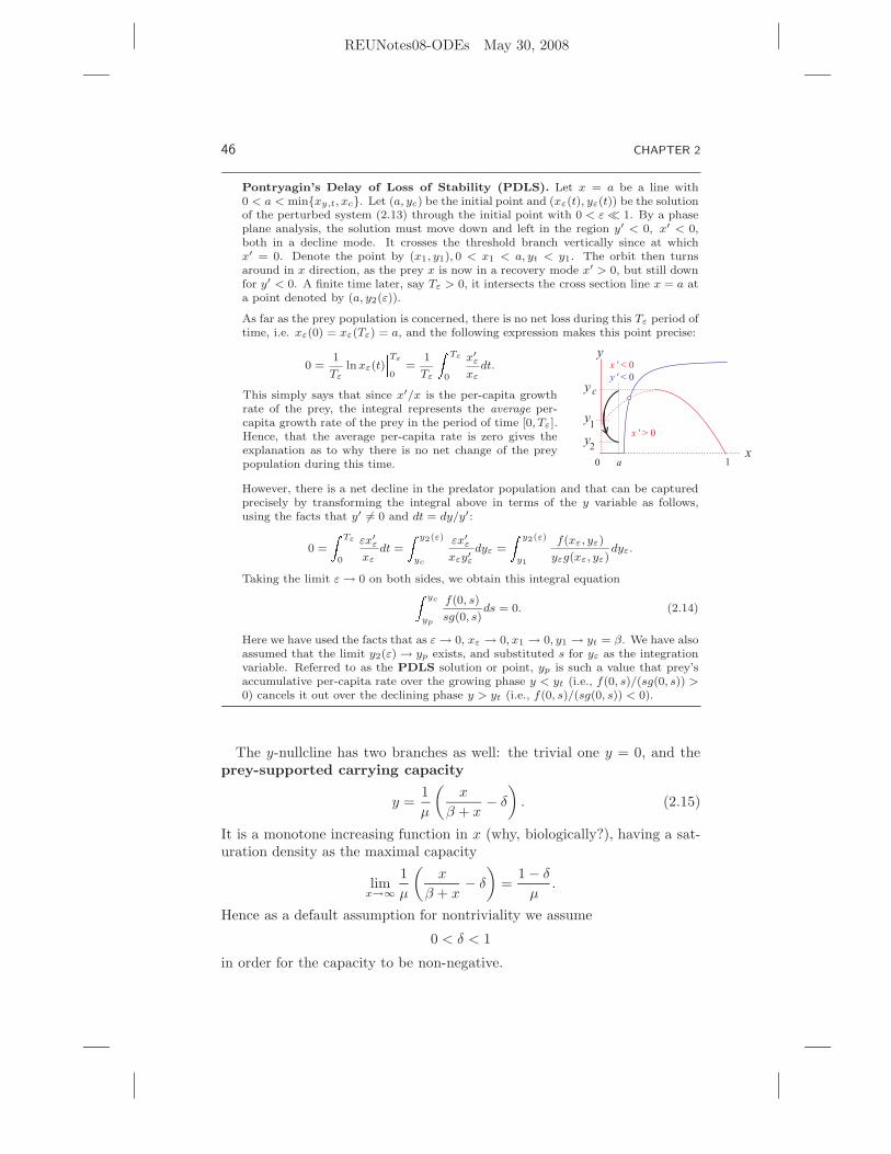
REUNotes08-ODEs May 30, 2008
46 CHAPTER 2
Pontryagin’s Delay of Loss of Stability (PDLS). Let x = a be a line with0 < a < min{xy,t, xc}. Let (a, yc) be the initial point and (xε(t), yε(t)) be the solutionof the perturbed system (2.13) through the initial point with 0 < ε ≪ 1. By a phaseplane analysis, the solution must move down and left in the region y′ < 0, x′ < 0,both in a decline mode. It crosses the threshold branch vertically since at whichx′ = 0. Denote the point by (x1, y1), 0 < x1 < a, yt < y1. The orbit then turnsaround in x direction, as the prey x is now in a recovery mode x′ > 0, but still downfor y′ < 0. A finite time later, say Tε > 0, it intersects the cross section line x = a ata point denoted by (a, y2(ε)).
As far as the prey population is concerned, there is no net loss during this Tε period oftime, i.e. xε(0) = xε(Tε) = a, and the following expression makes this point precise:
0 =1
Tε
lnxε(t)���Tε
0=
1
Tε
Z Tε
0
x′
ε
xε
dt.
This simply says that since x′/x is the per-capita growthrate of the prey, the integral represents the average per-capita growth rate of the prey in the period of time [0, Tε].Hence, that the average per-capita rate is zero gives theexplanation as to why there is no net change of the preypopulation during this time.
However, there is a net decline in the predator population and that can be capturedprecisely by transforming the integral above in terms of the y variable as follows,using the facts that y′ 6= 0 and dt = dy/y′:
0 =
Z Tε
0
εx′
ε
xε
dt =
Z y2(ε)
yc
εx′
ε
xεy′
ε
dyε =
Z y2(ε)
y1
f(xε, yε)
yεg(xε, yε)dyε.
Taking the limit ε → 0 on both sides, we obtain this integral equationZ yc
yp
f(0, s)
sg(0, s)ds = 0. (2.14)
Here we have used the facts that as ε → 0, xε → 0, x1 → 0, y1 → yt = β. We have alsoassumed that the limit y2(ε) → yp exists, and substituted s for yε as the integrationvariable. Referred to as the PDLS solution or point, yp is such a value that prey’saccumulative per-capita rate over the growing phase y < yt (i.e., f(0, s)/(sg(0, s)) >0) cancels it out over the declining phase y > yt (i.e., f(0, s)/(sg(0, s)) < 0).
The y-nullcline has two branches as well: the trivial one y = 0, and theprey-supported carrying capacity
y =1
µ
(
x
β + x− δ
)
. (2.15)
It is a monotone increasing function in x (why, biologically?), having a sat-uration density as the maximal capacity
limx→∞
1
µ
(
x
β + x− δ
)
=1 − δ
µ.
Hence as a default assumption for nontriviality we assume
0 < δ < 1
in order for the capacity to be non-negative.

REUNotes08-ODEs May 30, 2008
DIFFERENTIAL EQUATIONS 47
0 0.2 0.4 0.6 0.8 10
0.1
0.2
0.3
0.4
0.5
0.6
Prey x
Pre
da
tor y
ε = 0.05ε = 0.3
25 30 35 40 45 500
0.1
0.2
0.3
0.4
0.5
0.6
0.7
0.8
0.9
Time t
xy
ε = 0.05
0 0.2 0.4 0.6 0.8 1 1.2 1.40
0.05
0.1
0.15
0.2
0.25
0.3
0.35
0.4
0.45
0.5
ε
Ra
ng
e o
f y
yc
yt
(a) (b) (c)
Figure 2.9
The two branches intersects at a capacity transcritical point
(xy,t, yy,t) =
(
βδ
1 − δ, 0
)
.
It is the x-intercept point of the y-capacity branch (2.15).The combined configuration of the nullclines is such that the capacity
branch of the predator intersects the threshold branch of the prey. Thenecessary condition for this to happen is for the y capacity transcriticalvalue xy,t to lie below the crash-fold point xc:
xy,t =βδ
1 − δ<
1 − β
2= xc.
This is because the y capacity increases with increasing x, and as a result itwill not intersect the x-threshold branch if its minimal point (xy,t, 0) alreadylies above the right most point, (xc, yc), of the threshold branch. Given thisnecessary condition, a sufficient condition is for µ to be small. In fact,when µ = 0, the necessary condition is also sufficient because the y-capacitynullcline degenerates into a vertical line x = xy,t, going through the thresholdbranch of the prey.
Hence, to summarize the nullcline configuration for the analysis below, weassume
xy,t =βδ
1 − δ<
1 − β
2= xc and µ > 0 sufficient small.
Singular Cycle
Figure 2.8 illustrates the two limiting cases:(a) x is fast, y is slow when 0 < ε ≪ 1;(b) x is slow, y is fast when ε ≫ 1.
In (a), all singular orbits from the first quadrant converge to a limit cycle ofrelaxation oscillation which contains two fast orbits, initiating respectively atthe crash-fold point (xc, yc) and the PDLS point (0, yp). In (b), all singularorbits from the first quadrant converge to the coexisting xy-equilibrium state.

REUNotes08-ODEs May 30, 2008
48 CHAPTER 2
Figure 2.9 are computational simulations of the system. They are gener-ated for varying ε values but fixed values of the other parameters:
β = 0.2, δ = 0.2, µ = 1.
Fig.2.9(a) compares limit cycles for two different ε. The smaller ε is, thetighter the cycle is around the singular limit. Fig.2.9(b) is the time series plotfor one parameter value of ε. Notice that the prey population periodicallydips precariously too low. Fig.2.9(c) is a bifurcation diagram with ε beingthe bifurcation parameter. It is generated in the same way as the bifurcationdiagram for the FitzHugh-Nagumo circuit above. Again, a nonzero variationbetween the minimum and maximum implies a limit cycle, and the lack ofa variation means an equilibrium point. The Matlab m.file that generatesthe plot is PPbifurcation.m. Notice that the PDLS phenomenon is clearlyevident. That is, the rebounding (minimum) density of the predator liesbelow the transcritical bifurcation value yt. In contrast, the peak density isnear the saddle-node bifurcation value yc.
Exercises 2.5
1. Consider the equations (2.11) for the FitzHugh-Hagumo circuit. Assumethe IL-nullcline intersects the VC -nullcline only the latter’s branch left ofthe local minimum point. Sketch a phase portrait of singular orbits forthe two singular perturbation cases: (a) 0 < ε ≪ 1, (b) ε ≫ 1.
2. Consider the dimensionless predator-prey system (2.13) when β > 1, 0 <δ < 1 and xy,t < 1. Sketch a phase portrait of singular orbits for the twosingular perturbation cases: (a) 0 < ε ≪ 1, (b) ε ≫ 1.
3. Consider the dimensionless predator-prey system (2.13). In the case that0 < β < 1, 0 < δ < 1 and µ = 0, find the exact formula for the xy-equilibrium point.
4. The derivation of the PDLS point yp from the equation (2.14) does notdepends on the initial point yc. That is, one can start at any initialpoint (a, y0) with y0 > yt, and still derive the same form of the equationbelow for the corresponding PDLS point yp, which now is a function ofy0, yp = yp(y0):
∫ y0
yp
f(0, s)
sg(0, s)ds = 0.
Show that yp(y0) is a decreasing function of y0, and that limy0→∞ yp = 0.5. Show that the singular limit cycle of the predator-prey system (2.13) in
fact contains the crash-fold point (xc, yc) at ε = 0. (Hint: Modify thederivation of the PDLS point yp. More specifically, move the line x = acloser to the crash-fold point so that a < xc. Instead of starting atthe initial point (a, yc), start the orbit, (xε(t), yε(t)), at (a, y0) for anyy0 < yc. According the phase plane analysis, the orbit will cross the x-capacity nullcline at a point (x1(ε), y1(ε)), and then hit the line x = a ata point, (a, y2(ε)), with y2(ε) > yc. Then show limε→0 y2(ε) = yc.)

REUNotes08-ODEs May 30, 2008
DIFFERENTIAL EQUATIONS 49
2.6 LINEARIZATION
The phase line, phase plane, and time scale methods are both geometricaland global in nature. In this section however we turn our attention to amethod for the stability of equilibrium solutions that is analytical and localinstead. It is based on Taylor’s expansion of functions and the stabilityanalysis for linear equations from Sec.2.1.
The basic idea can be fixed by considering autonomous equations of 1variable
x′ = f(x).
The dynamics of the equation is captured completely by the phase linemethod as shown by example below.
In particular, the stability of all equilibrium points can be classified qual-itatively. Therefore, there is little to gain geometrically. However, if wewant to know how fast solutions converge to equilibrium a, for example,the phase line method is ineffective. Since such a question only concerns asmall interval of the equilibrium point a, we can simply ignore the vectorfield f outside the interval. If we keep zooming in at a, then the graph ofthe equation x′ = f(x) would look like a line—the tangent line of f(x) ata: x′ = f(a) + f ′(a)(x − a) = f ′(a)(x − a) since f(a) = 0. In other words,the original equation, which is usually nonlinear, is approximated to the firstorder by the following linear equation
x′ = f ′(a)(x − a)
which is called the linearization of the original equation at equilibrium a.
Property of Hyperbolicity: If f(q), f ′(q) 6= 0, then all essential infor-mation, geometrical and analytical, about the nonlinear equation near theequilibrium point q are preserved.
Take the case in the illustration that f ′(a) < 0 . Geometrically, f(x) > 0if and only if a−δ < x < a for a small δ > 0. Equivalently, f ′(a)(x−a) > 0 ifand only if x < a for the linearization. Therefore, the phase line structuresof both the nonlinear equation and its linearization near a is one of thesame. Most important of all, no small perturbations can change the overall

REUNotes08-ODEs May 30, 2008
50 CHAPTER 2
Higher Order Approximations. The idea of approximation prevails always. Takethe case in illustration as an example that is about the equilibrium point x = d.The linearization equation x′ = 0 would predict that all solutions near x = d areequilibrium solutions which clearly is false for the original equation. However, we canconsider the approximation that is one order higher than the tangent line approxi-mation of the vector field. More precisely, at the equilibrium point d at which thenonlinear vector field f has a quadratic-like tangency to the x-axis, the second orderTaylor’s approximation of the vector field is
f(x) ≈ f(d) + f ′(d)(x − d) +f ′′(d)
2!(x − d)2 =
f ′′(d)
2(x − d)2 6= 0
assuming f(d) = f ′(d) = 0 but f ′′(d) 6= 0. Thus the following equation
x′ =f ′′(d)
2(x − d)2
is an approximation of the nonlinear equation near x = d. It is a good approximationfor two reasons. Qualitatively it gives the same phase line structure near the pointas the original equation. Analytically, one can first check or derive by the methodof separation of variables the following solution to the initial value problem withx(0) = x0 of the approximating equation:
x(t) = d +x0 − d
1 − λ(x0 − d)t, with λ =
f ′′(d)
2.
Secondly, one can show that the difference between the exact soluiton, φ(t, x0), andthe approximate solution is of a smaller order than 1/|t| as t → ±∞.Similarly, for x = c at which f has a cubic-like tangency to the x-axis, the third orderTaylor’s approximation is used to derive the approximating equation
x′ =f ′′′(c)
3!(x − c)3,
assuming f(c) = f ′(c) = f ′′(c) = 0 but f ′′′(c) 6= 0. Again, one can use it to analyzethe original equation near x = c both geometrically and analytically.To summarize, linearization is simply a special but important case in the approxi-mation theory of differential equations. All degenerate cases, i.e. f(q) = f ′(q) = 0,are only secondary and exceptions to the hyperbolicity (i.e. f ′(q) 6= 0). Unlike thehyperbolicity, they can be removed by targeted perturbations to the equations.
qualitative structures of the equilibrium point, the essence of hyperbolicityby definition.
Analytically, we can solve the linearization equation explicitly as follows.If we let u = x − a as the new variable, then
u′ = (x − a)′ = x′ = f(a)(x − a) = f ′(a)u.
That is, the linearization equation is transformed into
u′ = λu
where λ = f ′(a) is a constant. Its general solution is given by
u(t) = Ceλt ⇐⇒ x(t) = a + Cef ′(a)t
Hence, for any initial point x0 from the interval (a − δ, a + δ), the solutionwith x(0) = x0 is given as
x(t) = a + (x0 − a)ef ′(a)t

REUNotes08-ODEs May 30, 2008
DIFFERENTIAL EQUATIONS 51
which converges to a exponentially fast. It is a theoretical fact that this solu-tion to the linearization approximates the solution to the original equation.The precise result can be stated as follows.
There is a sufficiently small δ > 0 so that for any initial point
x0 from the interval of I = (a − δ, a + δ), the solution denoted
by φ(t, x0) to initial value problem x′ = f(x), x(0) = x0 stays in
I for all t > 0 and the difference between the exact solution and
the linear approximation
|φ(t, x0) − [a + (x0 − a)ef ′(a)t]|
converges to zero at a rate faster than the exponential decay
ef ′(a)t as t → +∞.da
The case in illustration that f ′(b) > 0 is the same except that the exactand the approximate solution approach each other backward in time and ata rate faster than the exponential ef ′(b)t as t → −∞. To be precise,
limt→−∞
|φ(t, x0) − [b + (x0 − b)ef ′(b)t]|ef ′(b)t
= 0.
The linearization fails if f ′ = 0 at the equilibrium point, such as the casesin illustration for x = c and x = d. The linearization x′ = 0 is inconclusiveabout the dynamics of the nonlinear equation near these points. In such acase, higher order approximations of the vector field apply, see discussionfrom the inserted box.
We now extend the linearization method to 2-dimensional systems of equa-tions
{
x′ = f(x, y)
y′ = g(x, y).(2.16)
Assume (x, y) = (p, q) is an equilibrium point, i.e.,
f(p, q) = g(p, q) = 0,
and we want know the local stability of the equilibrium point as well as localsolution structure of the equation near the point. The principle rationaleof approximation is the same: solutions of the original equations are deter-mined by the vector field (f, g) their equations define, and as a result, anapproximating vector field of the exact vector field should give approximat-ing solutions to the exact solutions. This approach is particularly useful nearequilibrium points. The approximation is again based on Taylor’s approxi-mation of functions.

REUNotes08-ODEs May 30, 2008
52 CHAPTER 2
As the method goes, we approximate the vector field at the equilibriumpoint (p, q) by their tangent planes respectively as
f(x, y) ≈ f(p, q) +∂f
∂x(p, q)(x − p) +
∂f
∂y(p, q)(y − q)
=∂f
∂x(p, q)(x − p) +
∂f
∂y(p, q)(y − q)
g(x, y) ≈ g(p, q) +∂g
∂x(p, q)(x − p) +
∂g
∂y(p, q)(y − q)
=∂g
∂x(p, q)(x − p) +
∂g
∂y(p, q)(y − q).
The linear system of equations
x′ =∂f
∂x(p, q)(x − p) +
∂f
∂y(p, q)(y − q)
y′ =∂g
∂x(p, q)(x − p) +
∂g
∂y(p, q)(y − q).
is called the linearization of the original system at the equilibrium point(p, q).
To streamline notations, we use
a =∂f
∂x(p, q), b =
∂f
∂y(p, q)
c =∂g
∂x(p, q), d =
∂g
∂y(p, q),
u = x − p, v = y − q,
we rewrite the linearization as{
u′ = au + bv
v′ = cu + dv.(2.17)
The solution structure of this linear system and that of the original systemnear the equilibrium point (p, q) is now a matter of interpretation betweenthe two (2.16, 2.17).
Geometrical Properties of Linearization
First of all, the equilibrium point (p, q) of the original corresponds to thetrivial solution (0, 0) of the linearization. As a result, the origin of the (u, v)coordinate system is located at (p, q) on the (x, y) coordinate. Moreover,the u-axis is simply the translation of the x-axis to the point (p, q), and thesame for the v-axis and y-axis parallel.
More importantly, the u-nullcline
u′ = au + bv =∂f
∂x(p, q)(x − p) +
∂f
∂y(p, q)(y − q) = 0
is the precisely the tangent line of the x-nullcline
f(x, y) = 0

REUNotes08-ODEs May 30, 2008
DIFFERENTIAL EQUATIONS 53
at the equilibrium point (p, q). The most important of all is the propertythat both equations have the same sign polarity near the equilibrium point.This means that if the left side of the x-nullcline f(x, y) = 0 is where x′ > 0locally near the equilibrium point, then it is the left side of the u-nullclinethat is where u′ > 0. This is simply due to the fact that the u-equation isthe tangent plane approximation of the x-equation when both are viewed assurfaces, see the illustration below.
It is easy to see that u′ fails to capture the sign of x′ near the equilibriumpoint if u′ ≡ 0, that is, fx(p, q) = fy(p, q) = 0. In such a case, higher orderapproximation is required, which we will not pursue here.
The exactly same result and explanation apply to the y-equation and itslinearization v′ = cu + dv.
Let
J(p, q) =
[
∂f∂x (p, q) ∂f
∂y (p, q)∂g∂x(p, q) ∂g
∂y (p, q)
]
=
[
a bc d
]
which is referred to as the Jacobian of the vector field at point (p, q). Bydefinition, the equilibrium point (p, q) is said to be hyperbolic if J(p, q)does not have an eigenvalue whose real part is zero. (The real part of a realnumber is the real number itself.)
Topological Conjugacy: The geometrical structures of the nonlinear sys-tem and its linearization near a hyperbolic equilibrium point are the same(which has its technical definition called topological conjugacy). In partic-ular, the equilibrium point is stable for both systems or unstable for bothsystems.
Stability of Hyperbolic Equilibrium Points
The linearized system (2.17) can be written in a matrix form as(
uv
)
′
= J(p, q)
(
uv
)
.
From Sec.2.1 we know that the stability of its equilibrium point is determinedby the eigenvalues of the coefficient matrix J(p, q). Hence, we have thefollowing result
Stability Criteria: A hyperbolic equilibrium point (p, q) of the nonlinearsystem (2.16) is

REUNotes08-ODEs May 30, 2008
54 CHAPTER 2
• stable if the real parts of all eigenvalues of the Jacobian matrix J(p, q)are negative.
• unstable if the real part of one eigenvalue of the Jacobian matrix J(p, q)is positive.
Example 2.6.1 Use linearization to determine the stability of the equilib-rium point (0, 0) of the FitzHugh-Nagumo system
{
x′ = −x(x − a)(x − 1) − y
y′ = 2x − y,
where 0 < a < 1.
Solution: Let f(x, y) = −x(x − a)(x − 1) − y, g(x, y) = 2x − y. Then
J(0, 0) =
[
fx(0, 0) fy(0, 0)gx(0, 0) gy(0, 0)
]
=
[
−a −12 −1
]
.
The linearization of the system at (0, 0) is{
u′ = −au − v
v′ = 2u − v.
The characteristic equation is
|J(0, 0) − λI| = λ2 + (1 + a)λ + (a + 2) = 0.
The eigenvalues are
λ1,2 =−(1 + a) ±
√
(1 + a)2 − 4(a + 2)
2.
Since (1 + a)2 − 4(a + 2) = (1− a)2 − 8 < 0 when 0 < a < 1, the eigenvaluesare complex with real part −(1 + a)/2 < 0. Hence, the equilibrium point isstable for all 0 < a < 1.
da
The example above is one of such a case that it is not too hard to find theequilibrium point and the Jacobian explicitly and the linearization methodis then used directly. The following example is quite different. Finding theequilibrium and the Jacobian proves to be too tedious and too complex ifnot impossible when there is a simpler alternative. The key is to make useof geometrical properties of the linearization.
Example 2.6.2 Consider the dimensionless predator-prey model Eq.(2.13),which is recalled as follows.
εx′ = x(1 − x) − x
β + xy
y′ = y
(
x
β + x− δ − µy
)
.

REUNotes08-ODEs May 30, 2008
DIFFERENTIAL EQUATIONS 55
Consider also the following conditions
xy,t =βδ
1 − δ<
1 − β
2= xc and µ > 0 sufficient small.
so that if x is fast (0 < ε ≪ 1) the system has a singular attracting limitcycle and if x is slow (ε ≫ 1) the system has a singular stable equilibrium.(See Sec.2.5.) Use the method of linearization to determine how the stabilityof the xy-equilibrium point changes with the singular parameter ε.
Solution: Let{
εu′ = au + bv
v′ = cu + dv
be the linearization, where a = ∂f/∂x evalu-ated at an/the xy-equilibrium point and so on.We already know that the u-nullcine au+bv =0 is the tangent line to the x-nullcline at theequilibrium point. Since the tangent line hasa positive slope we have ab < 0. Since we alsoknow that u′ > 0 for (u, v) lies below the tangent line, we must have b < 0(why?). Hence we must have a > 0 and b < 0 as a result. Similarly, cd < 0because the v-nullcline has a positive slope. Again using the fact that v′ < 0for points above it, we conclude that c > 0, d < 0. Notice also that the slopof the v-nullcline, −c/d, is greater than the slope of the u-nullcline, −a/b.Thus,
−c/d > −a/b ⇐⇒ ad − bc > 0. (2.18)
The last inequality is obtained using the fact that b < 0, d < 0We now consider the eigenvalues of the Jacobian at the equilibrium point.
The characteristic equation is
det
∣
∣
∣
∣
aε − λ b
εc d − λ
∣
∣
∣
∣
= λ2 − (a
ε+ d)λ +
ad − bc
ε:= λ2 − Bλ + C
where for simpler notation we used
B =a
ε+ d, C =
ad − bc
ε.
Because a > 0, d < 0, B > 0 if ε ≪ 1 and B < 0 if ε ≫ 1. Also, because of(2.18), C > 0 and C ∼ +∞ if ε ≪ 1 and C ∼ 0 if ε ≫ 1. The eigenvaluesare
λ1,2 =B ±
√B2 − 4C
2.
We now see that
• For ε ≫ 1, B ∼ d < 0 and C ∼ 0+, implying λ1,2 < 0. Hence thexy-equilibrium point is stable.

REUNotes08-ODEs May 30, 2008
56 CHAPTER 2
• For ε ≪ 1, we have B ∼ +∞, C ∼ +∞, and B2 − 4C > 0 but√B2 − 4C < B. Hence, the xy-equilibrium point is a source, thus
unstable.•
In conclusion, as ε changes from very small to very large, the equilibriumpoint changes from being unstable to stable. This is consistent with thebifurcation plot of Fig.2.9(c) from the previous section.
da
Exercises 2.6
1. Some information of the linearization of a system of equations at an equi-librium point is given in each (a) and (b). Use the information to deter-mine the stability of the equilibrium point.
(a) (b)
2. Verify that x = 2 is an equilibrium solution of each equation. Use lin-earization to determine its stability.
(i) x′ = x3 − x2 − 2x
(ii) x′ = 3x − x2 − 3x
1 + x
3. Consider the system of two competing species{
x′ = x(3 − 3x − y)
y′ = y(2 − y − x).
Find the equilibrium point that is inside the first quadrant, and use lin-earization to determine its stability.
4. Find the equilibrium points of the system, and use linearization to deter-mine their stability.
{
x′ = 2x(1 − x2) − y
y′ = x − y.
5. Use linearization method to prove that the equilibrium point of Exercise1(a) above is always stable.

REUNotes08-ODEs May 30, 2008
DIFFERENTIAL EQUATIONS 57
6. Use linearization method to prove that the coexisting equilibrium pointof the model of two competing species Eq.(2.6) is always a saddle if noneof the species is competitive.