linear algebra in maple - applied mathematicsdjeffrey/offprints/k14662_c089.pdf · 89 linear...

89Linear Algebra

in Maple R©

David J. JeffreyThe University of Western Ontario

Robert M. CorlessThe University of Western Ontario

89.1 Introduction . . . . . . . . . . . . . . . . . . . . . . . . . . . . . . . . . . . . . . . . . 89-189.2 Vectors . . . . . . . . . . . . . . . . . . . . . . . . . . . . . . . . . . . . . . . . . . . . . . . 89-289.3 Matrices . . . . . . . . . . . . . . . . . . . . . . . . . . . . . . . . . . . . . . . . . . . . . 89-489.4 Arrays. . . . . . . . . . . . . . . . . . . . . . . . . . . . . . . . . . . . . . . . . . . . . . . . 89-889.5 Efficient Working with Vectors and Matrices . . 89-989.6 Equation Solving and Matrix Factoring . . . . . . . . . 89-12

89.7 Eigenvalues and Eigenvectors . . . . . . . . . . . . . . . . . . . . . 89-14

89.8 Linear Algebra with Modular Arithmetic . . . . . . . 89-15

89.9 Numerical Linear Algebra in Maple . . . . . . . . . . . . . 89-16

89.10 Canonical Forms. . . . . . . . . . . . . . . . . . . . . . . . . . . . . . . . . . . . 89-18

89.11 Structured Matrices . . . . . . . . . . . . . . . . . . . . . . . . . . . . . . . . 89-19

89.12 Functions of Matrices . . . . . . . . . . . . . . . . . . . . . . . . . . . . . . 89-21

89.13 Matrix Stability . . . . . . . . . . . . . . . . . . . . . . . . . . . . . . . . . . . . 89-23

References . . . . . . . . . . . . . . . . . . . . . . . . . . . . . . . . . . . . . . . . . . . . . . . . . . . . 89-24

89.1 Introduction

Maple R© is a general purpose computational system offering symbolic computation, exactand approximate (floating-point) numerical computation, and scientific plotting and graph-ics. The main Maple library is written in the Maple programming language, a rich languagethat allows easy access to advanced mathematical algorithms. A special feature of Maple isaccess for users to much of the library source code, including the ability to trace Maple’sown execution; the only parts of Maple that cannot be traced are those parts that arecompiled, for example, the kernel. Users can also link to lapack and nag library routinestransparently, and thus benefit from fast and reliable floating-point computation. Maplewas started in the early 1980s, and the Maplesoft company was founded in 1988.

There are two linear algebra packages in Maple: LinearAlgebra and linalg. The linalgpackage is older and is considered obsolete; it was replaced by LinearAlgebra in Maple 6.We describe here only the LinearAlgebra package, as contained in Maple 17. The readershould be careful when reading other reference books, or the Maple help pages, to checkwhether the functions being discussed include the obsolete functions vector, matrix,

array (notice the lower-case initial letter) of the older package, or include Vector, Matrix,

Array (with an upper-case initial letter), which are part of the newer package.Maple’s LinearAlgebra package uses a strict data typing based on the notions of abstract

linear algebra [Jac53]. There are strict distinctions between scalars, vectors, matrices, andarrays, of which users should be aware. Another feature of Maple’s linear algebra arisesbecause of the additional considerations that are required in the context of symbolic com-putation. These considerations are usually omitted from standard texts, and are the subjectof additional comments here.

89-1

89-2 Handbook of Linear Algebra

Facts:

1. Maple offers a number of interface options, including the two GUI interfaces “Work-sheet mode” and “Document mode”, and also a non-GUI command-line interface. Weconcentrate here on the Maple 17 worksheet mode.

2. Maple commands are typed after a prompt symbol, which by default is [>, or just>. In examples below, keyboard input is simulated by prefixing the actual commandtyped with the prompt symbol >.

3. In Maple examples below, white space is used to enhance readability. Maple ignoresextra spaces. Also, comments within the code are preceded by # .

4. In some of the examples below, a command is too long to fit on one line. In worksheetmode, shift-enter continues to a new line, and no continuation character is printed; incommand-line Maple, the continuation character backslash ( \ ) is used. Here we usethe worksheet convention. When typing long examples into Maple, either shift-entercan be typed when the end of the line as printed here is reached, or one can ignorethe new line and continue typing, allowing Maple to wrap the command.

5. Maple commands are terminated by either semicolon ( ; ) or colon ( : ). The semicolonallows the output of a command to be displayed; the colon suppresses the outputdisplay, but the command still executes. Before Maple 10, one of the two commandterminators was required, but starting in the Maple 10 GUI a carriage return isequivalent to semicolon, when the default 2-D input is used.

6. To access the commands described below, load the LinearAlgebra package by typingthe command (after the prompt, as shown)> with( LinearAlgebra );

If the package is not loaded, then either a typed command will not be recognized,or a different command with the same name will be used.

7. The results of a command can be assigned to one or more variables. Thus,> a := 1 ;

assigns the value 1 to the variable a, while> (a,b,c) := 1,2,3 ;

assigns a the value 1, b the value 2 and c the value 3.Caution: The operator “colon-equals” ( := ) is assignment, while the operator “equals”( = ) defines an equation with a left-hand side and a right-hand side.

8. A sequence of expressions separated by commas is an expression sequence in Maple,and some commands return expression sequences, which can be assigned as above.

9. Ranges in Maple are generally defined using a pair of periods ( .. ). The rules for theranges of subscripts are given below.

10. Output format in Maple uses spaces to separate elements in vectors and matrices,but here for space saving we also use commas.

89.2 Vectors

Facts:

1. In Maple, vectors are not just lists of elements. Maple separates the idea of themathematical object Vector from the data object Array (see Section 89.4).

2. A Maple Vector can be converted to an Array, and an Array of appropriate shapecan be converted to a Vector, but they cannot be used interchangeably in commands.See the help file for convert to find out about other conversions.

3. Maple distinguishes between column vectors, the default, and row vectors. The twotypes of vectors behave differently, and are not merely presentational alternatives.

Linear Algebra in Maple 89-3

Commands:

1. Generation of vectors:

• Vector( [x1, x2, . . .] ) Construct a column vector by listing its elements. The length of

the list specifies the dimension.

• Vector[column]( [x1, x2, . . . ] ) Explicitly declare the column attribute.

• Vector[row]( [x1, x2, . . . ] ) Construct a row vector by initializing its elements from a

list.

• <v1, v2, . . .> Construct a column vector with elements v1, v2, etc. An element can be

another column vector.

• <v1|v2| . . . > Construct a row vector with elements v1, v2, etc. An element can be another

row vector. A useful mnemonic is to think of the bars, | , as column dividers in a table.

• Vector( n, k−>f(k) ). Construct an n-dimensional vector using a function f(k) to de-

fine the elements. f(k) is evaluated sequentially for k from 1 to n. The notation k−>f(k)is Maple syntax for a univariate function.

• Vector( n, fill=v ) An n-dimensional vector with every element equal to v.

• Vector( n, symbol=v ) An n-dimensional vector containing symbolic components vk.

• map( x−>f(x), V ) Construct a new vector by applying function f(x) to each element

of the vector named V. Caution: the command is map not Map. Several Maple packages,

including LinearAlgebra, define a command Map, but the command map is easier to use.

• RandomVector( n, generator= a .. b) Construct a vector with random integer entries

taken from the interval [a, b]. The default is [−99, 99].

2. Operations and functions:

• v[i] Element i of vector v. The result is a scalar. Caution: A symbolic reference v[i] is

typeset as vi on output in a Maple worksheet.

• v[p..q] Vector consisting of elements vi, p ≤ i ≤ q. The result is a Vector, even for the

case v[p..p]. Either of p or q can be negative, meaning that the location is found by

counting backward from the end of the vector, with −1 being the last element.

• u+v, u-v Add or subtract Vectors u, v.

• a∗v Multiply vector v by scalar a. Notice the operator is “asterisk” (∗).• u . v, DotProduct( u, v ) The inner product of Vectors u and v. See examples for

complex conjugation rules. Notice the operator is “period” (.) not “asterisk” (∗) because

inner product is not commutative over the field of complex numbers.

• Transpose( v ), v∧ %T Change a column vector into a row vector, or vice versa.

Complex elements are not conjugated.

• HermitianTranspose( v ), v∧ %H Transpose with complex conjugation.

• OuterProductMatrix( u, v ) The outer product of Vectors u and v (ignoring the at-

tributes of row or column).

• CrossProduct( u, v ), u &x v The vector product, or cross product, of three-

dimensional vectors u, v.

• Norm( v ) The infinity norm of a vector v. The infinity norm is chosen rather than the

2-norm because in a symbolic context the infinity norm is usually easier to compute and

it leads to less unwieldy expressions than the 2-norm.

• Norm( v, 2 ) The 2-norm or Euclidean norm of vector v. Notice that the second argu-

ment, namely the 2, is necessary, because Norm( v ) is the infinity norm, which is different

from the default in many textbooks and software packages.

• Norm( v, p ) The p-norm of v, namely (∑ni=1 |vi|

p)(1/p) .


Examples:

In Example 5 below, the imaginary unit is the Maple default I. That is,√−1 = I. In the matrix

section, we show how this can be changed. To save space, we shall mostly use row vectors.

1. Generate vectors. The same vector created different ways.

> Vector[row]([0,3,8]): <0|3|8>: Transpose(<0,3,8>): Vector[row]

(3,i->i∧2-1);

[0, 3, 8]

2. Selecting elements.

> V := <a|b|c|d|e|f>: V1 := V[2 .. 4]; V2 := V[-4 .. -1];

V3 := V[-4 .. 4];

V 1 := [b, c, d] , V 2 := [c, d, e, f ] , V 3 := [c, d]

3. A Gram–Schmidt exercise.

> u1 := <3|0|4>: u2 := <2|1|1>: w1n := u1/Norm( u1, 2 );

w1n := [3/5, 0, 4/5]

> w2 := u2 - (u2 . w1n)∗w1n; w2n := w2/Norm( w2, 2 );

w2n :=

[2√

2

5,

√2

2, −3

√2

10

]4. Comparison of norms in a symbolic setting:

> V:= Vector( 1,3,x,y): [ Norm(V), Norm(V,2) ] ;[max(3, |x|, |y|),

√10 + |x|2 + |y|2

]5. Vectors with complex elements. Define column vectors uc,vc and row vectors ur,vr.

> uc := <1 + I,2>: ur := Transpose( uc ): vc := <5,2 − 3*I>:

vr := Transpose( vc ):

The inner product of column vectors conjugates the first vector in the product, and the

inner product of row vectors conjugates the second.

> inner1 := uc . vc; inner2 := ur . vr;

inner1 := 9-11 I , inner2 := 9+11 I

Maple computes the product of two similar vectors, i.e., both rows or both columns, as

a true mathematical inner product, since that is the only definition possible; in contrast, if

the user mixes row and column vectors, then Maple does not conjugate:

> but := ur . vc; but := 9− ICaution: The use of a period (.) with complex row and column vectors together differs from the

use of a period (.) with complex 1 × m and m × 1 matrices. In case of doubt, use matrices and

conjugate explicitly where desired.

89.3 Matrices

Facts:1. One-column matrices and vectors are not interchangeable in Maple.2. Matrices and two-dimensional arrays are not interchangeable in Maple.

Commands:

1. Generation of Matrices. This can be done using either the Matrix command or using angle

bracket notation << . . . >>. Owing to recent improvements in Maple, they are of compa-

rable efficiency.


• Matrix( [[a, b, . . .],[c, d, . . .],. . .] ) Construct a matrix row-by-row, using a list of lists.

• < a, b, . . . ; c, d, . . . ; . . . > Construct a matrix using Matlab-style syntax.

• << a|b|. . .>,<c|d|. . .>,. . .> Construct a matrix row-by-row using vectors. Notice that

the rows are specified by row vectors, requiring the | notation.

• << a,b,. . .>|< c,d,. . .>|. . .> Construct a matrix column-by-column using vectors. No-

tice that each vector is a column, and the columns are joined using | .• Matrix( n, m, (i,j)−>f(i,j) ) Construct a matrix n ×m using a function f(i, j) to

define the elements. f(i, j) is evaluated sequentially for i from 1 to n and j from 1 to m.

The notation (i,j)−>f(i,j) is Maple syntax for a bivariate function f(i, j).

• Matrix( n, m, fill=a ) An n×m matrix with each element equal to a.

• Matrix( n, m, symbol=a ) An n×m matrix containing subscripted entries aij .

• map( x−>f(x), M ) A matrix obtained by applying f(x) to each element of M .

Caution: the command is map not Map. See comment in Section 89.2.

• << A | B>, < C | D>> Construct a partitioned (block) matrix from matricesA,B,C,D.

Note that < A|B > will be formed by adjoining columns; the block < C|D > will be placed

below < A|B >. The Maple syntax is similar to a common textbook notation for parti-

tioned matrices.

• RandomMatrix( n, m, generator=a .. b) Generate a matrix with random integer entries

taken from the interval [a, b]. The default is [−99, 99].

2. Operations and functions

• M[i,j] Element i, j of matrix M . The result is a scalar.

• M[1..−1,k] Column k of Matrix M . The result is a Vector.

• M[k,1..−1] Row k of Matrix M . The result is a row Vector.

• M[p..q,r..s] Matrix consisting of submatrix mij , p ≤ i ≤ q, r ≤ j ≤ s. In Handbook

notation, M [{p, . . . , q}, {r, . . . , s}].• M[RowList,ColList] Matrix with rows and columns specified by the lists (order respected).

• Transpose( M ), M∧ %T Transpose matrix M , without taking the complex conjugate of

the elements.

• HermitianTranspose( M ), M∧ %H Transpose matrix M , taking the complex conjugate

of elements.

• A ± B Add/subtract compatible matrices or vectors A, B.

• A . B Product of compatible matrices or vectors A, B. The examples give details of how

Maple interprets products, since there are differences from other software packages.

• MatrixInverse( A ), A∧(−1) Inverse of matrix A.

• Determinant( A ) Determinant of matrix A.

• Norm( A ) The infinity norm of the matrix A. In a symbolic context, this norm is more

practical than the 2-norm (see example).

• Norm( A, 2 ) The (subordinate) 2-norm of matrix A, namely max‖u‖2 =1 ‖Au‖2 where

the norm in the definition is the vector 2-norm.

Cautions:

(a) Notice that the second argument, i.e., 2, is necessary because Norm( A ) is the infinity

norm, which is different from the default in many textbooks and software packages.

(b) Notice also that this is the largest singular value of A, and is usually different from the

Frobenius norm ‖A‖F , accessed by Norm( A, Frobenius ), which is the Euclidean

norm of the vector of elements of the matrix A.


(c) UnlessA has floating-point entries, this norm usually will not be computable explicitly,

and it may be expensive even to try.

• Norm( A, p ) The (subordinate) matrix p-norm of A, for integers p >= 1 or for p being

the symbol infinity. , which is the default value.

Examples:

1. A matrix product.

> A := <<1|−2|3>,<0|1|1>>; B := Matrix(3, 2, symbol=b); C := A . B;

A :=

[1 −2 3

0 1 1

], B :=

b11 b12

b21 b22

b31 b32

,C :=

[b11 − 2b21 + 3b31 b12 − 2b22 + 3b32

b21 + b31 b22 + b32

].

2. A Gram–Schmidt calculation revisited.

If u1, u2 are m × 1 column matrices, then the Gram–Schmidt process is often written in

textbooks asw2 = u2 −

uT2 u1

uT1 u1u1.

Notice, however, that uT2 u1 and uT1 u1 are strictly 1 × 1 matrices. Textbooks often slide

effortlessly over the conversion of uT2 u1 from a 1× 1 matrix to a scalar. Maple, in contrast,

does not suppose that conversion should be automatic.

Transcribing the printed formula into Maple will cause an error. Here is the way to do it.

We reuse the earlier numerical data.

> u1 := <<3,0,4>>; u2 := <<2,1,1>>; r := u2^%T . u1;

s := u1^%T . u1;

u1 :=

3

0

4

, u2 :=

2

1

1

, r := [10] , s := [25].

Notice the brackets in the values of r and s; they show us that r and s are matrices. Since

r[1,1] and s[1,1] are scalars, we can write

> w2 := u2 - r[1,1]/s[1,1]*u1;

and reobtain the result from Example 89.2.3. Alternatively, u1 and u2 can be converted to

Vectors first and then used to form a proper scalar inner product.

> r := u2[1..−1,1] . u1[1..−1,1]; s := u1[1..−1,1] . u1[1..−1,1]; w2 := u2-r/s*u1;

r := 10 , s := 25 , w2 :=

4/5

1

−3/5

.3. Vector–Matrix and Matrix–Vector products.

Many textbooks treat a column vector and a one-column matrix as equivalent, but this is

not so in Maple. Thus,

> b := <1,2>; B := <<1,2>>; C := <<4|5|6>>;

b :=

[1

2

]B :=

[1

2

]C :=

[4 5 6

].

Only the product B . C is defined, and the product b . C causes an error.

> B . C [4 5 6

8 10 12

].


The rules for mixed products are

Vector[row]( n ) . Matrix( n, m ) = Vector[row]( m )

Matrix( n, m ) . Vector[column]( m ) = Vector[column]( n )

The combinations Vector(n). Matrix(1, m) and Matrix(m, 1). Vector[row](n) cause

errors. If users do not want this level of rigor, then the easiest thing to do is to use only the

Matrix declaration.

4. Comparison of norms in a symbolic setting. The matrix A:=Matrix([[1,2],[3,x]]) has

the infinity-norm Norm(A) equal to 3 + |x| whereas Norm(A,2) is already an expression too

lengthy to reproduce here.

5. Working with matrices containing complex elements.

First, notation: In linear algebra, I is commonly used for the identity matrix. This corre-

sponds to the eye function in MATLAB. However, by default, Maple uses I for the imaginary

unit, as seen in Section 89.2. We can, however, use I for an identity matrix by changing the

imaginary unit to something else, say _i.

> interface( imaginaryunit=_i):

As the saying goes: An _i for an I and an I for an eye.

Now we can calculate eigenvalues using notation similar to introductory textbooks.

> A := <<1,2>|<-2,1>>; I := IdentityMatrix( 2 );

p := Determinant ( x*I-A );

A :=

[1 −2

2 1

], I :=

[1 0

0 1

], p := x2 − 2x+ 5.

Solving p = 0, we obtain eigenvalues 1+2i, 1−2i. With the above setting of imaginaryunit,

Maple will print these values as 1+2 _i, 1-2 _i, but we have translated back to standard

mathematical i, where i2 = −1.

6. Moore–Penrose inverse. Consider the following 3 × 2 matrix M , which contains a symbolic

parameter a.

M =

1 1

a a2

a2 a

.

We compute its Moore–Penrose pseudoinverse and a proviso guaranteeing correctness by the

command

>(Mi, p):= MatrixInverse(M, method=pseudo, output=[inverse, proviso]);

which assigns the 2× 3 pseudoinverse to Mi and an expression which, if nonzero, guarantees

that Mi is the correct (unique) Moore–Penrose pseudoinverse of M . Here we have

Mi :=

(2 + 2 a3 + a2 + a4

)−1−

a3 + a2 + 1

a (a5 + a4 − a3 − a2 + 2 a− 2)

a4 + a3 + 1

a (a5 + a4 − a3 − a2 + 2 a− 2)(2 + 2 a3 + a2 + a4

)−1 a4 + a3 + 1

a (a5 + a4 − a3 − a2 + 2 a− 2)−

a3 + a2 + 1

a (a5 + a4 − a3 − a2 + 2 a− 2)

and p = a2−a. Thus, if a 6= 0 and a 6= 1, the computed pseudoinverse is correct. By separate

computations we find that the pseudoinverse of M |a=0 is[1/2 0 0

1/2 0 0

]and that the pseudoinverse of M |a=1 is[

1/6 1/6 1/6

1/6 1/6 1/6

]


and moreover that these are not special cases of the generic answer returned previously. The

Moore–Penrose inverse is one example of a linear algebra function that is discontinuous,

even for square matrices. We give more examples below.

89.4 Arrays

Before describing Maple’s Array structure, it is useful to say why Maple distinguishesbetween an Array and a Vector or Matrix, when other books and software systems do not.In linear algebra, two different types of operations are performed with vectors or matrices.The first type is described in Sections 89.2 and 89.3, and comprises operations derived fromthe mathematical structure of vector spaces. The other type comprises operations that treatvectors or matrices as data arrays; they manipulate the individual elements directly. As anexample, consider dividing the elements of Array [1, 3, 5] by the elements of [7, 11, 13] toobtain [1/7, 3/11, 5/13].

The distinction between the operations can be made in either of two places: in thename of the operation or the name of the object. In other words, we can overload eitherdata objects or operators. Systems such as Matlab choose to leave the data object un-changed, and define separate operators. Thus, in Matlab the statements [1, 3, 5]/[7, 11, 13]and [1, 3, 5]./[7, 11, 13] are different because the operators are different. In contrast, Maplechooses to make the distinction in the data object, as will now be described.

Facts:

1. The Maple Array is a general data structure akin to arrays in other programminglanguages.

2. An array can have up to 63 indices and each index can lie in any integer range.3. The description here only addresses the overlap between Maple Array and Vector.

Caution: A Maple Array might look the same as a vector or matrix when printed.

Commands:

1. Generation of arrays.

• Array([x1, x2, . . .]) Construct an array by listing its elements.

• Array( m..n ) Declare an empty one-dimensional array indexed from m to n.

• Array( v ) Use an existing Vector to generate an array.

• convert( v, Array ) Convert a Vector v into an Array. Similarly, a Matrix can

be converted to an Array. See the help file for rtable options for advanced methods to

convert efficiently, in-place.

2. Operations (memory/stack limitations may restrict operations).

• a ∧ n Raise each element of a to power n.

• a ∗ b, a + b, a − b Multiply (add, subtract) elements of b by (to, from) elements

of a.

• a / b Divide elements of a by elements of b. Division by zero will produce undefined or

infinity (or exceptions can be caught by user-set traps; see the help file for Numeric Events).

Examples:

1. Array arithmetic.


> simplify( (Array([25,9,4])*Array(1..3,x->x∧2-1 )/Array(<5,3,2>\ ))∧(1/2));

[0, 3, 4]

2. Getting Vectors and Arrays to do the same thing.

> Transpose( map(x->x∗x,<1,2,3> )) - convert(Array( [1,2,3] )∧2, Vector);

[0, 0, 0]

89.5 Efficient Working with Vectors and Matrices

We point out here some aspects of the linear algebra package that are important for workingwith, and programming, Maple efficiently.

Facts:

1. Saving a copy of a matrix in Maple is different from many other computationalpackages. Consider this attempt to save a copy of matrix A in matrix B beforealtering A:> A:=<< 1 | 2 | 3 >>: # Create a 1-by-3 matrix

> B:=A: # Store before modification

> A[1,1]:= -100: # Modify the first entry

> B;

[−100, 2, 3]

The reason for the matrix B changing along with A is that the statement B:=A equatesthe storage addresses of the two matrices, and thus both names point to the samelocation and any change to one will be reflected in the other. The intention of theuser was to store a separate copy of the matrix A before modifying it. The way to dothis is the following.

> A:=<< 1 | 2 | 3 >>: # Create the 1-by-3 matrix as before

> B:=Copy(A) : # Store a copy before modification

> A[1,1]:= -100: # Modify the first entry

> B; A;

[ 1, 2, 3]

[-100, 2, 3]

2. A puzzle will arise for a user who wants to construct a matrix by modifying an iden-tity matrix, and tries > eye := IdentityMatrix(3,3);1 0 0

0 1 0

0 0 1

> eye[1,2]:=4;

Error: invalid assignment

Maple by default stores an identity matrix in a compact form which has no room foradditional elements. To obtain the desired action, proceed> aye := IdentityMatrix(3,3,compact=false);1 0 0

0 1 0

0 0 1


> aye[1,2]:=4; aye

1 4 0

0 1 0

0 0 1

3. Editing and Visualization. By default, the Maple interface writes out explicitly only

matrices smaller than 10 × 10, and otherwise prints a summary of the matrix di-mensions and datatype. If a user wishes to inspect a large matrix, there are severaloptions. Submatrices of size 10× 10 or less will print explicitly. Alternatively, a usercan right-click on the output summary and select Browse from the menu. Elementscan then be interactively edited and the edited matrix is saved on exit. If the editedmatrix has been assigned to a name, the stored matrix will contain the edited ele-ments. The Browse window also offers an image tab which uses greyscale or colors tovisualize the structure of a matrix.

4. Programming with submatrices. In some computation systems, replacing explicit pro-gramming loops with submatrix operations gives efficiency gains. In addition to effi-ciency, many authors, for example [GV96], describe their algorithms using submatri-ces. In Maple, however, using submatrices does not increase efficiency because Maplemakes a copy of each submatrix before executing any requested operation. As anexample, the reader can enter the code below and execute it with his or her ownmatrices. Even without explicit timing, the speed differences will be clear for largermatrices.Suppose we wish to illustrate matrix multiplication as an explicit program, ratherthan use the built-in operation. This function calculates element by element:

mult1 := proc (A, B) local i, j, k, C, arow, acol, brow, bcol;

(arow, acol) := Dimension(A); (brow, bcol) := Dimension(B);

C := Matrix(arow, bcol);

for i to arow do

for j to bcol do

C[i, j] := add(A[i, k]*B[k, j], k = 1 .. acol);

end do;

end do;

return(C);

end proc;

This one uses submatrix operations to multiply a row by a column:

mult2 := proc (A, B) local i, j, C, arow, acol, brow, bcol;

(arow, acol) := Dimension(A); (brow, bcol) := Dimension(B);

C := Matrix(arow, bcol);

for i to arow do

for j to bcol do

C[i, j] := A[i, 1 .. -1].B[1 .. -1, j]

end do;

end do;

return(C);

end proc;


89.6 Equation Solving and Matrix Factoring

Cautions:

1. If a matrix contains exact numerical entries, typically integers or rationals, then thematerial studied in introductory textbooks transfers to a computer algebra systemwithout special considerations. However, if a matrix contains symbolic entries, thenthe fact that computations are completed without the user seeing the intermediatesteps can lead to unexpected results.

2. Some of the most popular matrix functions are discontinuous when applied to matricescontaining symbolic entries. Examples are given below.

3. Some algorithms taught to educate students about the concepts of linear algebra oftenturn out to be ill-advised in practice: computing the characteristic polynomial andthen solving it to find eigenvalues, for example; using Gaussian elimination withoutpivoting on a matrix containing floating-point entries, for another.

Commands:

1. LinearSolve( A, B ) The vector or matrix X satisfying AX = B. If B is a vector, so is

X; otherwise, they are matrices.

2. BackwardSubstitute( A, B ), ForwardSubstitute( A, B ) The vector or matrixX sat-

isfying AX = B when A is in upper or lower triangular (echelon) form, respectively.

3. ReducedRowEchelonForm( A ) The reduced row-echelon form (RREF) of the matrix A.

For matrices with symbolic entries, see the examples below for recommended usage.

4. Rank( A ) The rank of the matrix A. Caution: If A has floating-point entries, see the

section below on Numerical Linear Algebra. On the other hand, if A contains symbolic

entries, then the rank may change discontinuously and the generic answer returned by Rank

may be incorrect for some specializations of the parameters.

5. NullSpace( A ) The nullspace (kernel) of the matrix A. Caution: If A has floating-point

entries, see Section 89.9. Again, on the other hand, if A contains symbolic entries, the

nullspace may change discontinuously and the generic answer returned by NullSpace may

be incorrect for some specializations of the parameters.

6. ( P, L, U, R ) := LUDecomposition( A, method=’RREF’ ) The PLUR, or Turing, fac-

tors of the matrix A. See examples for usage.

7. ( P, L, U ) := LUDecomposition( A ) The PLU factors of a matrix A, when the RREF

R is not needed. This is usually the case for a Turing factoring where R is guaranteed (or

known a priori) to be I, the identity matrix, for all values of the parameters.

8. ( Q, R ) := QRDecomposition( A, fullspan ) The QR factors of the matrix A. The

option fullspan ensures that Q is square.

9. SingularValues( A ) See Section 89.9.

10. ConditionNumber( A ) See Section 89.9.

Examples:

1. The need for Turing factoring.

One of the strengths of Maple is computation with symbolic quantities. When standard

linear algebra methods are applied to matrices containing symbolic entries, the user must

be aware of new mathematical features that can arise. The main feature is the discontinuity

of standard matrix functions, such as the reduced row-echelon form and the rank, both of

which can be discontinuous. For example, the matrix

B = A− λI =

[7− λ 4

6 2− λ

]


has the reduced row-echelon form

ReducedRowEchelonForm(B) =

[1 0

0 1

]λ 6= −1, 10

[1 −4/3

0 0

]λ = 10,

[1 1/2

0 0

]λ = −1.

Notice that the function is discontinuous precisely at the interesting values of λ. Computer

algebra systems in general, and Maple in particular, return “generic” results. Thus, in Maple,

we have

> B := << 7-x | 4 >, < 6 | 2-x >>;

B :=

[7− x 4

6 2− x

],

> ReducedRowEchelonForm( B ) [1 0

0 1

].

This difficulty is discussed at length in [CJ92] and [CJ97]. The recommended solution is to

use Turing factoring (generalized PLU decomposition) to obtain the reduced row-echelon

form with provisos. Thus, for example,

> A := <<1|-2|3|sin(x)>,<1|4*cos(x)|3|3*sin(x)>,<-1|3|cos(x)-3|cos(x)>>;

A :=

1 −2 3 sinx

1 4 cosx 3 3 sinx

−1 3 cosx− 3 cosx

.> ( P, L, U, R ) := LUDecomposition( A, method=’RREF’ ):

The generic reduced row-echelon form is then given by

R =

1 0 0 (2 sinx cosx− 3 sinx− 6 cosx− 3)/(2 cosx+ 1)

0 1 0 sinx/(2 cosx+ 1)

0 0 1 (2 cosx+ 1 + 2 sinx)/(2 cosx+ 1)

This shows a visible failure when 2 cosx+ 1 = 0, but the other discontinuity is invisible, and

one requires the U factor from the Turing (PLUR) factors,

U =

1 −2 3

0 4 cosx+ 2 0

0 0 cosx

to see that the case cosx = 0 also causes failure. In both cases (meaning the cases cosx = 0

and 2 cosx+ 1 = 0), the RREF must be recomputed to obtain the singular cases correctly.

2. QR factoring.

Maple does not offer column pivoting, so in pathological cases the factoring may not be

unique, and will vary between software systems. For example,

> A := <<0,0>|<5,12>>: QRDecomposition( A, fullspan )[5/13 12/13

12/13 −5/13

],

[0 13

0 0

].


89.7 Eigenvalues and Eigenvectors

Facts:

1. In exact arithmetic, explicit expressions are not possible in general for the eigenvaluesof a matrix of dimension 5 or higher.

2. When it has to, Maple represents polynomial roots (and, hence, eigenvalues) implic-itly by the RootOf construct. Expressions containing RootOfs can be simplified andevaluated numerically.

Commands:

1. Eigenvalues( A ) The eigenvalues of matrix A.

2. Eigenvectors( A ) The eigenvalues and corresponding eigenvectors of A.

3. CharacteristicPolynomial( A, ’x’ ) The characteristic polynomial of A expressed us-

ing the variable x.

4. JordanForm( A ) The Jordan form of the matrix A.

Examples:

1. Simple eigensystem computation.

> Eigenvectors( <<7,6>|<4,2>> );[−1

10

],

[−1/2 4/3

1 1

].

So the eigenvalues are−1 and 10 with the corresponding eigenvectors [−1/2, 1]T and [4/3, 1]T .

2. A defective matrix.

If the matrix is defective, then by convention the matrix of “eigenvectors” returned by Maple

contains one or more columns of zeros.

> Eigenvectors( <<1,0>|<1,1>> ); [1

1

],

[1 0

0 0

].

3. Larger systems.

For larger matrices, the eigenvectors will use the Maple RootOf construction. Consider

A :=

3 1 7 1

5 6 −3 5

3 −1 −1 0

−1 5 1 5

.> ( L, V ) := Eigenvectors( A ): The colon suppresses printing. The vector of

eigenvalues is returned as

> L; RootOf

(Z 4 − 13 Z 3 − 4 Z 2 + 319 Z − 386, index = 1

)RootOf

(Z 4 − 13 Z 3 − 4 Z 2 + 319 Z − 386, index = 2

)RootOf

(Z 4 − 13 Z 3 − 4 Z 2 + 319 Z − 386, index = 3

)RootOf

(Z 4 − 13 Z 3 − 4 Z 2 + 319 Z − 386, index = 4

).

This, of course, simply reflects the characteristic polynomial:

> CharacteristicPolynomial( A, ’x’ );

x4 − 13x3 − 4x2 + 319x− 386


The Eigenvalues command solves a 4th degree characteristic polynomial explicitly in

terms of radicals unless the option implicit is used.

4. Jordan form. Caution: As with the reduced row-echelon form, the Jordan form of a matrix

containing symbolic elements can be discontinuous. For example, given

A =

[1 t

0 1

],

> ( J, Q ) := JordanForm( A, output=[’J’,’Q’] );

J,Q :=

[1 1

0 1

],

[t 0

0 1

]with A = QJQ−1. Note that Q is invertible precisely when t 6= 0. This gives a proviso on

the correctness of the result: J will be the Jordan form of A only for t 6= 0, which we see is

the generic case returned by Maple.

Caution: Exact computation has its limitations, even without symbolic entries. If we ask

for the Jordan form of the matrix

B =

−1 4 −1 −14 20 −8

4 −5 −63 203 −217 78

−1 −63 403 −893 834 −280

−14 203 −893 1703 −1469 470

20 −217 834 −1469 1204 −372

−8 78 −280 470 −372 112

,

a relatively modest 6×6 matrix with a triple eigenvalue 0, then the transformation matrix Q

as produced by Maple has entries over 35,000 characters long. Some scheme of compression

or large expression management is thereby mandated.

89.8 Linear Algebra with Modular Arithmetic

There is a subpackage, LinearAlgebra[Modular], designed for programmatic use, thatoffers access to modular arithmetic with matrices and vectors.

Facts:

1. The subpackage can be loaded by issuing the command> with( LinearAlgebra[Modular] ); which gives access to the commands

[AddMultiple, Adjoint, BackwardSubstitute, Basis, Characteristic

Polynomial, ChineseRemainder, Copy, Create, Determinant, Fill,

ForwardSubstitute, Identity, Inverse, LUApply, LUDecomposition,

LinIntSolve, MatBasis, MatGcd, Mod, Multiply, Permute, Random,

Rank, RankProfile, RowEchelonTransform, RowReduce, Swap,

Transpose, ZigZag]

2. Arithmetic can be done modulo a prime p or, in some cases, a composite modulus m.3. The relevant matrix and vector datatypes are integer[4], integer[8], integer[],

and float[8]. Use of the correct datatype can improve efficiency.

Examples:

> p := 13;

> A := Mod( p, Matrix([[1,2,3],[4,5,6],[7,8,-9]]), integer[4] );


1 2 3

4 5 6

7 8 4

,> Mod( p, MatrixInverse( A ), integer[4] );12 8 5

0 11 3

5 3 5

Cautions:

1. This is not to be confused with the mod utilities, which together with the inert Inverse

command can also be used to calculate inverses in a modular way.

2. One must always specify the datatype in Modular commands, or a cryptic error message will

be generated.

89.9 Numerical Linear Algebra in Maple

The previous sections have covered the use of Maple for exact computations of the types metduring a standard first course on linear algebra. However, in addition to exact computation,Maple offers a variety of floating-point numerical linear algebra support.

Facts:

1. Maple can compute with either “hardware floats” or “software floats.”2. A hardware float is IEEE double precision, with a mantissa of (approximately) 15

decimal digits.3. A software float has a mantissa whose length is set by the Maple variable Digits.

Cautions:

1. If an integer is typed with a decimal point, then Maple treats it as a software float.2. Software floats are significantly slower that hardware floats, even for the same preci-

sion.

Commands:

1. Matrix( n, m, datatype=float[8] ) An n×m matrix of hardware floats (initialization

data not shown). The elements must be real numbers. The 8 refers to the number of bytes

used to store the floating point real number.

2. Matrix( n, m, datatype=complex(float[8] )) An n×m matrix of hardware floats, in-

cluding complex hardware floats. A complex hardware float takes two 8-byte storage loca-

tions.

3. Matrix( n, m, datatype=sfloat ) An n×m matrix of software floats. The entries must

be real and the precision is determined by the value of Digits.

4. Matrix( n, m, datatype=complex(sfloat) ) As before with complex software floats.

5. Matrix( n, m, shape=symmetric ) A matrix declared to be symmetric. Maple can take

advantage of shape declarations such as this.

Examples:

1. A characteristic surprise.

When asked to compute the characteristic polynomial of a floating-point matrix, Maple first

computes eigenvalues (by a good numerical method) and then presents the characteristic


polynomial in factored form, with good approximate roots. Thus,

> A:= Matrix( 2, 2, [[666,667],[665,666]],datatype=float[8]):

> CharacteristicPolynomial( A, ’x’ )

(x− 1331.99924924882612− 0.0 i) (x− 0.000750751173882235889− 0.0 i) .

Notice the signed zero in the imaginary part; though the roots in this case are real, approxi-

mate computation of the eigenvalues of a nonsymmetric matrix takes place over the complex

numbers. (n.b.: The output above has been edited for clarity.)

2. Symmetric matrices.

If Maple knows that a matrix is symmetric, then it uses appropriate routines. Without the

symmetric declaration, the calculation is

> Eigenvalues( Matrix( 2, 2, [[1,3],[3,4]], datatype=float[8]) );[−0.854101966249684707 + 0.0 i

5.85410196624968470 + 0.0 i

].

With the declaration, the computation is

> Eigenvalues( Matrix( 2, 2, [[1,3],[3,4]], shape=symmetric,

datatype=float[8]) ); [−0.854101966249684818

5.85410196624968470

].

Cautions: Use of the shape=symmetric declaration will force Maple to treat the matrix as

being symmetric, even if it is not.

3. Printing of hardware floats.

Maple prints hardware floating-point data as 18-digit numbers. This does not imply that all

18 digits are correct; Maple prints the hardware floats this way so that a cycle of converting

from binary to decimal and back to binary will return to exactly the starting binary floating-

point number. Notice in the previous example that the last three digits differ between the

two function calls. In fact, neither set of digits is correct, as a calculation in software floats

with higher precision shows:

> Digits := 30: Eigenvalues( Matrix( 2, 2, [[1,3],[3,4]], \

datatype=sfloat, shape=symmetric ) );[−0.854101966249684544613760503093

5.85410196624968454461376050310

].

4. NullSpace. Consider

> B := Matrix( 2, 2, [[666,667],[665,666]] ): A := Transpose(B).B;

We make a floating-point version of A by

> Af := Matrix( A, datatype=float[8] );

and then take the NullSpace of both A and Af. The nullspace of A is correctly returned as

the empty set — A is not singular (in fact, its determinant is 1). The nullspace of Af is

correctly returned as {[−0.707637442412755612

0.706575721416702662

]}.

The answers are different — quite different — even though the matrices differ only in

datatype. The surprising thing is that both answers are correct: Maple is doing the right

thing in each case. See [Cor93] for a detailed explanation, but note that Af times the vector

in the reported nullspace is about 3.17 · 10−13 times the 2-norm of Af.


5. Approximate Jordan form (not!).1

As noted previously, the Jordan form is discontinuous as a function of the entries of the

matrix. This means that rounding errors may cause the computed Jordan form of a matrix

with floating-point entries to be incorrect, and for this reason Maple refuses to compute the

Jordan form of such a matrix.

6. Conditioning of eigenvalues.

To explore Maple’s facilities for the conditioning of the unsymmetric matrix eigenproblem,

consider the matrix “gallery(3)” from Matlab.

> A := Matrix( [[-149,-50,-154], [537,180,546], [-27,-9,-25]] ):

The Maple command EigenConditionNumbers computes estimates for the reciprocal con-

dition numbers of each eigenvalue, and estimates for the reciprocal condition numbers of the

computed eigenvectors as well. At this time, there are no built-in facilities for the computa-

tion of the sensitivity of arbitrary invariant subspaces.

> E,V,rconds,rvecconds := EigenConditionNumbers( A, output=

[’values’, ’vectors’,’conditionvalues’,’conditionvectors’] ):

> seq( 1/rconds[i], i=1..3 );

417.6482708, 349.7497543, 117.2018824

A separate computation using the definition of the condition number of an eigentriplet

(y∗, λ,x) (see Chapter 21) as

Cλ =‖y∗‖∞‖x‖∞|y∗ · x|

gives exact condition numbers (in the infinity norm) for the eigenvalues 1, 2, 3 as 399, 252,

and 147. We see that the estimates produced by EigenConditionNumbers are of the right

order of magnitude.

89.10 Canonical Forms

There are several canonical forms in Maple: Jordan form, Smith form, Hermite form, andFrobenius form, to name a few. In this section, we talk only about the Smith form (definedin Section 6.6 and Section 32.2).

Commands:

1. SmithForm( B, output=[’S’,’U’,’V’] ) Smith form of B.

Examples:

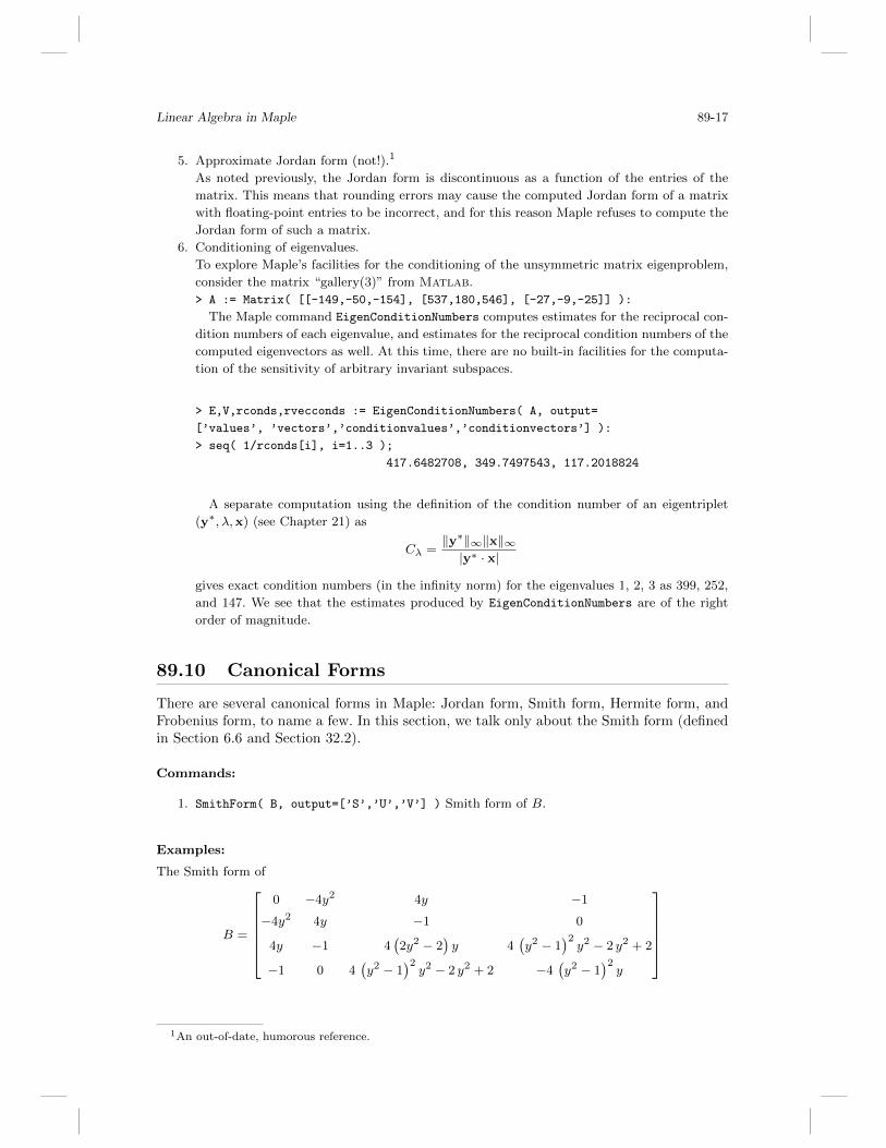
The Smith form of

B =

0 −4y2 4y −1

−4y2 4y −1 0

4y −1 4(2y2 − 2

)y 4

(y2 − 1

)2y2 − 2 y2 + 2

−1 0 4(y2 − 1

)2y2 − 2 y2 + 2 −4

(y2 − 1

)2y

1An out-of-date, humorous reference.


is

S =

1 0 0 0

0 1 0 0

0 0 1/4(2y2 − 1

)20

0 0 0 (1/64)(2 y2 − 1

)6

.Maple also returns two unimodular (over the domain Q[y]) matrices U and V for which A = U.S.V .

89.11 Structured Matrices

Facts:

1. Computer algebra systems are particularly useful for computations with structuredmatrices.

2. User-defined structures may be programmed using index functions. See the help pagesfor details.

3. Examples of built-in structures include symmetric, skew-symmetric, Hermitian, Van-dermonde, and Circulant matrices.

Examples:

Generalized Companion Matrices. Maple can deal with several kinds of generalized companion

matrices. A generalized companion matrix2 pencil of a polynomial p(x) is a pair of matrices C0, C1

such that det(xC1−C0) = 0 precisely when p(x) = 0. Usually, in fact, det(xC1−C0) = p(x), though

in some definitions proportionality is all that is needed. In the case C1 = I, the identity matrix,

we have C0 = C(p(x)) is the companion matrix of p(x). Matlab’s roots function computes roots

of polynomials by first computing the eigenvalues of the companion matrix, a venerable procedure

only recently proved stable.

The generalizations allow direct use of alternative polynomial bases, such as the Chebyshev

polynomials, Lagrange polynomials, Bernstein (Bezier) polynomials, and many more. Further, the

generalizations allow the construction of generalized companion matrix pencils for matrix polyno-

mials, allowing one to easily solve nonlinear eigenvalue problems.

We give three examples below.

If p := 3+2x+x2, then CompanionMatrix( p, x ) produces “the” (standard) companion matrix

(also called Frobenius form companion matrix):[0 −3

1 −2

]and it is easy to see that det(tI − C) = p(t). If instead

p := B30(x) + 2B3

1(x) + 3B32(x) + 4B3

3(x)

where Bnk (x) =(nk

)(1− x)n−k(x+ 1)k/2n is the kth Bernstein (Bezier) polynomial of degree n on

the interval −1 ≤ x ≤ 1, then CompanionMatrix( p, x ) produces the pencil (note that this is not

in Frobenius form)

C0 =

−3/2 0 −4

1/2 −1/2 −8

0 1/2 −52

3

2Sometimes known as “colleague” or “comrade” matrices, an unfortunate terminology that inhibits key-

word search.


C1 =

3/2 0 −4

1/2 1/2 −8

0 1/2 −20

3

(from a formula by Jonsson and Vavasis [JV05] and independently by Winkler [Win04]), and we

have p(x) = det(xC1 − C0). Note that the program does not change the basis of the polynomial

p(x) of Eq. (89.9) to the monomial basis (it turns out that p(x) = 20 + 12x in the monomial basis,

in this case: note that C1 is singular). It is well known that changing polynomial bases can be

ill-conditioned, and this is why the routine avoids making the change.

Next, if we choose nodes [−1,−1/3, 1/3, 1] and look at the degree 3 polynomial taking the values

[1,−1, 1,−1] on these four nodes, then CompanionMatrix( values, nodes ) gives C0 and C1 where

C1 is the 5× 5 identity matrix with the (5, 5) entry replaced by 0, and

C0 =

1 0 0 0 −1

0 1/3 0 0 1

0 0 −1/3 0 −1

0 0 0 −1 1

− 9

16

27

16−27

16

9

160

.

We have that det(tC1 − C0) is of degree 3 (in spite of these being 5 × 5 matrices), and that

this polynomial takes on the desired values ±1 at the nodes. Therefore, the finite eigenvalues of

this pencil are the roots of the given polynomial. See [CW04] and [Cor04], for example, for more

information.

Finally, consider the nonlinear eigenvalue problem below: find the values of x such that the

matrix C with Cij = T0(x)/(i+ j+ 1) +T1(x)/(i+ j+ 2) +T2(x)/(i+ j+ 3) is singular. Here Tk(x)

means the kth Chebyshev polynomial, Tk(x) = cos(k cos−1(x)). We issue the command

> ( C0, C1 ) := CompanionMatrix( C, x );

from which we find

C0 =

0 0 0 −2/15 −1/12 − 2

35

0 0 0 −1/12 − 2

35−1/24

0 0 0 − 2

35−1/24 − 2

631 0 0 −1/4 −1/5 −1/6

0 1 0 −1/5 −1/6 −1/7

0 0 1 −1/6 −1/7 −1/8

and

C1 =

1 0 0 0 0 0

0 1 0 0 0 0

0 0 1 0 0 0

0 0 0 2/5 1/3 2/7

0 0 0 1/3 2/7 1/4

0 0 0 2/7 1/4 2/9

.

This uses a formula from [Goo61], extended to matrix polynomials. The six generalized eigenvalues

of this pencil include, for example, one near to −0.6854 + 1.909i. Substituting this eigenvalue in

for x in C yields a three-by-three matrix with ratio of smallest to largest singular values σ3/σ1 ≈1.7 · 10−15. This is effectively singular and, thus, we have found the solutions to the nonlinear


eigenvalue problem. Again note that the generalized companion matrix is not in Frobenius standard

form, and that this process works for a variety of bases, including the Lagrange basis.

Circulant matrices and Vandermonde matrices.

> A := Matrix( 3, 3, shape=Circulant[a,b,c] );a b c

c a b

b c a

,> F3 := Matrix( 3,3,shape=Vandermonde[[1,exp(2*Pi*I/3),exp(4*Pi*I/3)]] );1 1 1

1 −1/2 + 1/2 i√

3(−1/2 + 1/2 i

√3)2

1 −1/2− 1/2 i√

3(−1/2− 1/2 i

√3)2.

It is easy to see that the F3 matrix diagonalizes the circulant matrix A.

Toeplitz and Hankel matrices. These can be constructed by calling ToeplitzMatrix and

HankelMatrix, or by direct use of the shape option of the Matrix constructor.

> T := ToeplitzMatrix( [a,b,c,d,e,f,g] );

> T := Matrix( 4,4,shape=Toeplitz[false,Vector(7,[a,b,c,d,e,f,g])] );

both yield a matrix that looks like d c b a

e d c b

f e d c

g f e d

,though in the second case only 7 storage locations are used, whereas 16 are used in the first. This

economy may be useful for larger matrices. The shape constructor for Toeplitz also takes a Boolean

argument true, meaning symmetric.

Both Hankel and Toeplitz matrices may be specified with an indexed symbol for the entries:

> H := Matrix( 4, 4, shape=Hankel[a] ); yieldsa1 a2 a3 a4

a2 a3 a4 a5

a3 a4 a5 a6

a4 a5 a6 a7

.

89.12 Functions of Matrices

The exponential of the matrix A is computed in the MatrixExponential command of Mapleby polynomial interpolation (see Section 17.1) of the exponential at each of the eigenvalues ofA, including multiplicities. In an exact computation context, this method is not so “dubious”[MV78, Lab97]. This approach is also used by the general MatrixFunction command.

Examples:

> A := Matrix( 3, 3, [[-7,-4,-3],[10,6,4],[6,3,3]] ):

> MatrixExponential( A ); 6− 7 e1 3− 4 e1 2− 3 e1

10 e1 − 6 −3 + 6 e1 −2 + 4 e1

6 e1 − 6 −3 + 3 e1 −2 + 3 e1

(89.1)


Now a square root: > MatrixFunction( A, sqrt(x), x ):−6 −7/2 −5/2

8 5 3

6 3 3

(89.2)

Another matrix square root example, for a matrix close to one that has no square root:

> A := Matrix( 2, 2, [[epsilon∧2, 1], [0, delta∧2] ] ):

> S := MatrixFunction( A, sqrt(x), x ):

> simplify( S ) assuming positive; [ε

1

ε+ δ

0 δ

](89.3)

If ε and δ both approach zero, we see that the square root has an entry that approaches infinity.

Calling MatrixFunction on the above matrix with ε = δ = 0 yields an error message, Matrix

function x∧(1/2) is not defined for this Matrix, which is correct.

Now for the matrix logarithm.

> Pascal := Matrix( 4, 4, (i,j)->binomial(j-1,i-1) );1 1 1 1

0 1 2 3

0 0 1 3

0 0 0 1

(89.4)

> MatrixFunction( Pascal, log(x), x );0 1 0 0

0 0 2 0

0 0 0 3

0 0 0 0

(89.5)

Now a function not covered in Chapter 17, instead of redoing the sine and cosine examples:

> A := Matrix( 2, 2, [[-1/5, 1], [0, -1/5]] ):

> W := MatrixFunction( A, LambertW(-1,x), x );

W :=

LambertW(−1,−1/5) −5LambertW (−1,−1/5)

1 + LambertW (−1,−1/5)

0 LambertW (−1,−1/5)

(89.6)

> evalf( W ); [−2.542641358 −8.241194055

0.0 −2.542641358

](89.7)

That matrix satisfies W exp(W ) = A, and is a primary matrix function. See [CGH+96] for more

details about the Lambert W function, and [CDH07] for more details on matrix W.

Now the matrix sign function (cf. Section 17.7). Consider

> Pascal2 := Matrix( 4, 4, (i,j)->(-1)∧(i-1)*binomial(j-1,i-1) );1 1 1 1

0 −1 −2 −3

0 0 1 3

0 0 0 −1

. (89.8)


Then we compute the matrix sign function of this matrix by

> S := MatrixFunction( Pascal2, csgn(z), z ): which turns out to be the same matrix (Pascal2).

Note: The complex “sign” function we use here is not the usual complex sign function for scalars

signum(reiθ) := eiθ,

but rather (as desired for the definition of the matrix sign function)

csgn(z) =

1 if Re(z) > 0

−1 if Re(z) < 0

signum(Im(z)) if Re(z) = 0

.

This has the side effect of making the function defined even when the input matrix has purely

imaginary eigenvalues. The signum and csgn of 0 are both 0, by default, but can be specified

differently if desired.

Cautions:

1. Further, it is not the sign function in Maple, which is a different function entirely: That

function (sign) returns the sign of the leading coefficient of the polynomial input to sign.

2. (In general) This general approach to computing matrix functions can be slow for large exact

or symbolic matrices (because manipulation of symbolic representations of the eigenvalues

using RootOf, typically encountered for n ≥ 5, can be expensive), and on the other hand

can be unstable for floating-point matrices, as is well known, especially those with nearly

multiple eigenvalues. However, for small or for structured matrices this approach can be very

useful and can give insight.

89.13 Matrix Stability

As defined in Chapter 26, a matrix is (negative) stable if all its eigenvalues are in the lefthalf-plane (in this section, “stable” means “negative stable”). In Maple, one may test thisby direct computation of the eigenvalues (if the entries of the matrix are numeric) and thisis likely faster and more accurate than any purely rational operation based test such as theHurwitz criterion. If, however, the matrix contains symbolic entries, then one usually wishesto know for what values of the parameters the matrix is stable. We may obtain conditionson these parameters by using the Hurwitz command of the PolynomialTools package onthe characteristic polynomial.

Examples:

Negative of gallery(3) from MATLAB.

> A := -Matrix( [[-149,-50,-154], [537,180,546], [-27,-9,-25]] ):

> E := Matrix( [[130, -390, 0], [43, -129, 0], [133,-399,0]] ):

> AtE := A - t*E; 149− 130 t 50 + 390 t 154

−537− 43 t −180 + 129 t −546

27− 133 t 9 + 399 t 25

(89.9)

For which t is that matrix stable?

> p := CharacteristicPolynomial( AtE, lambda );

> PolynomialTools[Hurwitz]( p, lambda, ’s’, ’g’ );

This command returns “FAIL,” meaning that it cannot tell whether p is stable or not; this is

only to be expected as t has not yet been specified. However, according to the documentation, all

coefficients of λ returned in s must be positive in order for p to be stable. The coefficients returned


are [λ

6 + t, 1/4

(6 + t)2 λ

15 + 433453 t+ 123128 t2,

(60 + 1733812 t+ 492512 t2

)λ

(6 + t) (6 + 1221271 t)

](89.10)

and analysis (not given here) shows that these are all positive if and only if t > −6/1221271.

Acknowledgments

Many people have contributed to linear algebra in Maple, for many years. Dave Hare andDavid Linder deserve particular credit, especially for the LinearAlgebra package and itsconnections to CLAPACK, and have also greatly helped our understanding of the best wayto use this package. We are grateful to Dave Linder and to Jurgen Gerhard for commentson early drafts of this chapter.

References

[Cor93] R.M. Corless. Six, lies, and calculators. Am. Math. Month., 100(4): 344–350, 1993.

[Cor04] R.M. Corless. Generalized companion matrices in the Lagrange basis. In L. Gonzalez-

Vega and T. Recio, Eds., Proc. EACA, pp. 317–322, June 2004.

[CDH+07] R.M. Corless, H. Ding, N.J. Higham, and D.J. Jeffrey. The solution of S*exp(S)=A

is not always the Lambert W function of A. In: ISSAC 2007, C.W. Brown, Ed., pp.

116–121, ACM Press, 2007.

[CGH+96] R.M. Corless, G.H. Gonnet, D.E.G. Hare, D.J. Jeffrey, and D.E. Knuth. On the

Lambert W function. Adv. Comp. Math., 5: 329–359, 1996.

[CJ92] R.M. Corless and D.J. Jeffrey. Well... it isn’t quite that simple. SIGSAM Bull., 26(3):

2–6, 1992.

[CJ97] R.M. Corless and D.J. Jeffrey. The Turing factorization of a rectangular matrix. SIGSAMBull., 31(3): 20–28, 1997.

[CW04] R.M. Corless and S.M. Watt. Bernstein bases are optimal, but, sometimes, Lagrange

bases are better. In Proc. SYNASC, pp. 141–153. Mirton Press, September 2004.

[GV96] G.H. Golub and C.F. Van Loan. Matrix Computations, 3rd ed. Johns Hopkins Press,

Baltimore, MD, 1996.

[Goo61] I.J. Good. The colleague matrix, a Chebyshev analogue of the companion matrix. Q. J.Math., 12: 61–68, 1961.

[Jac53] N. Jacobson. Lectures in Abstract Algebra. II Linear Algebra. Van Nostrand, New

York, 1953.

[JV05] G.F. Jonsson and S. Vavasis. Solving polynomials with small leading coefficients. SIAMJ. Matrix Anal. Appl., 26(2): 400–414, 2005.

[Lab97] G. Labahn, Personal Communication, 1997.

[MV78] C. Moler and C. Van Loan. Nineteen dubious ways to compute the exponential of a

matrix. SIAM Rev., 20(4): 801–836, 1978.

[Win04] J.R. Winkler. The transformation of the companion matrix resultant between the power

and Bernstein polynomial bases. Appl. Num. Math., 48(1): 113–126, 2004.

linear algebra in maple - applied mathematicsdjeffrey/offprints/k14662_c089.pdf · 89 linear...

Documents