linear algebra - bucks county community...

Linear Algebra

Joe Erickson

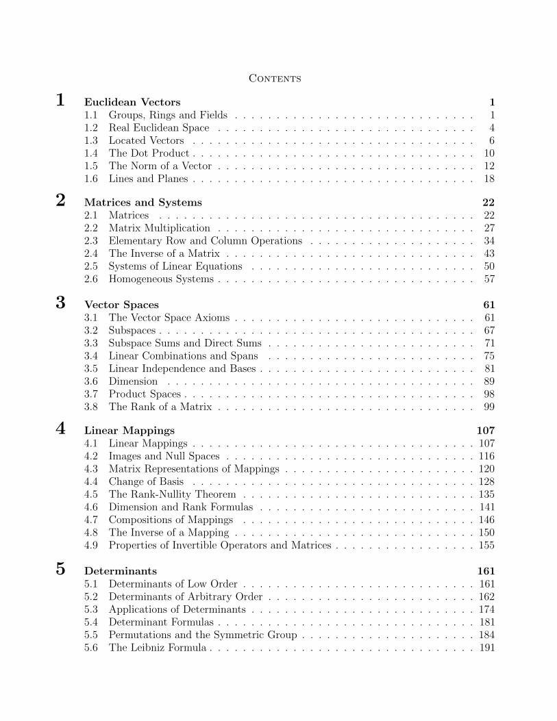
Contents

1 Euclidean Vectors 11.1 Groups, Rings and Fields . . . . . . . . . . . . . . . . . . . . . . . . . . . . . 11.2 Real Euclidean Space . . . . . . . . . . . . . . . . . . . . . . . . . . . . . . . 41.3 Located Vectors . . . . . . . . . . . . . . . . . . . . . . . . . . . . . . . . . . 61.4 The Dot Product . . . . . . . . . . . . . . . . . . . . . . . . . . . . . . . . . . 101.5 The Norm of a Vector . . . . . . . . . . . . . . . . . . . . . . . . . . . . . . . 121.6 Lines and Planes . . . . . . . . . . . . . . . . . . . . . . . . . . . . . . . . . . 18

2 Matrices and Systems 222.1 Matrices . . . . . . . . . . . . . . . . . . . . . . . . . . . . . . . . . . . . . . 222.2 Matrix Multiplication . . . . . . . . . . . . . . . . . . . . . . . . . . . . . . . 272.3 Elementary Row and Column Operations . . . . . . . . . . . . . . . . . . . . 342.4 The Inverse of a Matrix . . . . . . . . . . . . . . . . . . . . . . . . . . . . . . 432.5 Systems of Linear Equations . . . . . . . . . . . . . . . . . . . . . . . . . . . 502.6 Homogeneous Systems . . . . . . . . . . . . . . . . . . . . . . . . . . . . . . . 57

3 Vector Spaces 613.1 The Vector Space Axioms . . . . . . . . . . . . . . . . . . . . . . . . . . . . . 613.2 Subspaces . . . . . . . . . . . . . . . . . . . . . . . . . . . . . . . . . . . . . . 673.3 Subspace Sums and Direct Sums . . . . . . . . . . . . . . . . . . . . . . . . . 713.4 Linear Combinations and Spans . . . . . . . . . . . . . . . . . . . . . . . . . 753.5 Linear Independence and Bases . . . . . . . . . . . . . . . . . . . . . . . . . . 813.6 Dimension . . . . . . . . . . . . . . . . . . . . . . . . . . . . . . . . . . . . . 893.7 Product Spaces . . . . . . . . . . . . . . . . . . . . . . . . . . . . . . . . . . . 983.8 The Rank of a Matrix . . . . . . . . . . . . . . . . . . . . . . . . . . . . . . . 99

4 Linear Mappings 1074.1 Linear Mappings . . . . . . . . . . . . . . . . . . . . . . . . . . . . . . . . . . 1074.2 Images and Null Spaces . . . . . . . . . . . . . . . . . . . . . . . . . . . . . . 1164.3 Matrix Representations of Mappings . . . . . . . . . . . . . . . . . . . . . . . 1204.4 Change of Basis . . . . . . . . . . . . . . . . . . . . . . . . . . . . . . . . . . 1284.5 The Rank-Nullity Theorem . . . . . . . . . . . . . . . . . . . . . . . . . . . . 1354.6 Dimension and Rank Formulas . . . . . . . . . . . . . . . . . . . . . . . . . . 1414.7 Compositions of Mappings . . . . . . . . . . . . . . . . . . . . . . . . . . . . 1464.8 The Inverse of a Mapping . . . . . . . . . . . . . . . . . . . . . . . . . . . . . 1504.9 Properties of Invertible Operators and Matrices . . . . . . . . . . . . . . . . . 155

5 Determinants 1615.1 Determinants of Low Order . . . . . . . . . . . . . . . . . . . . . . . . . . . . 1615.2 Determinants of Arbitrary Order . . . . . . . . . . . . . . . . . . . . . . . . . 1625.3 Applications of Determinants . . . . . . . . . . . . . . . . . . . . . . . . . . . 1745.4 Determinant Formulas . . . . . . . . . . . . . . . . . . . . . . . . . . . . . . . 1815.5 Permutations and the Symmetric Group . . . . . . . . . . . . . . . . . . . . . 1845.6 The Leibniz Formula . . . . . . . . . . . . . . . . . . . . . . . . . . . . . . . . 191

6 Eigen Theory 1946.1 Eigenvectors and Eigenvalues . . . . . . . . . . . . . . . . . . . . . . . . . . . 1946.2 The Characteristic Polynomial . . . . . . . . . . . . . . . . . . . . . . . . . . 2006.3 Applications of the Characteristic Polynomial . . . . . . . . . . . . . . . . . . 2116.4 Similar Matrices . . . . . . . . . . . . . . . . . . . . . . . . . . . . . . . . . . 2166.5 The Theory of Diagonalization . . . . . . . . . . . . . . . . . . . . . . . . . . 2196.6 Diagonalization Methods and Applications . . . . . . . . . . . . . . . . . . . 2266.7 Matrix Limits and Markov Chains . . . . . . . . . . . . . . . . . . . . . . . . 2316.8 The Cayley-Hamilton Theorem . . . . . . . . . . . . . . . . . . . . . . . . . . 232

7 Inner Product Spaces 2377.1 Inner Products . . . . . . . . . . . . . . . . . . . . . . . . . . . . . . . . . . . 2377.2 Norms . . . . . . . . . . . . . . . . . . . . . . . . . . . . . . . . . . . . . . . . 2437.3 Orthogonal Bases . . . . . . . . . . . . . . . . . . . . . . . . . . . . . . . . . 2487.4 Quadratic Forms . . . . . . . . . . . . . . . . . . . . . . . . . . . . . . . . . . 259

8 Operator Theory 2668.1 The Adjoint of a Linear Operator . . . . . . . . . . . . . . . . . . . . . . . . 2668.2 Self-Adjoint and Unitary Operators . . . . . . . . . . . . . . . . . . . . . . . 2698.3 Normal Operators . . . . . . . . . . . . . . . . . . . . . . . . . . . . . . . . . 2768.4 The Spectral Theorem . . . . . . . . . . . . . . . . . . . . . . . . . . . . . . . 278

9 Canonical Forms 2849.1 Generalized Eigenvectors . . . . . . . . . . . . . . . . . . . . . . . . . . . . . 2849.2 Jordan Form . . . . . . . . . . . . . . . . . . . . . . . . . . . . . . . . . . . . 287

10 The Geometry of Vector Spaces 28810.1 Convex Sets . . . . . . . . . . . . . . . . . . . . . . . . . . . . . . . . . . . . 288

Appendix 293Symbol Glossary . . . . . . . . . . . . . . . . . . . . . . . . . . . . . . . . . . . . . . 293

1

1Euclidean Vectors

1.1 – Groups, Rings and Fields

It is assumed that the reader is well familiar with sets and functions. Given a set S, abinary operation from S ×S to S is a function ∗ : S ×S → S, so that for each (a, b) ∈ S ×Swe have ∗(a, b) ∈ S. As is customary we will usually write a ∗ b instead of ∗(a, b). The operation∗ is commutative if, for every a, b ∈ S,

∗(a, b) = a ∗ b = b ∗ a = ∗(b, a),

and associative if, for every a, b, c ∈ S,

∗(a, ∗(b, c)) = a ∗ (b ∗ c) = (a ∗ b) ∗ c = ∗(∗(a, b), c).

Common binary operations are addition of real numbers, + : R× R→ R, and multiplicationof real numbers, · : R× R→ R, both of which are commutative and associative. Recall thatsubtraction and division of real numbers is neither commutative nor associative, and indeeda÷ b is not even defined in the case when b = 0!

Linear algebra is foremost the study of vector spaces, and the functions between vectorspaces called mappings. However, underlying every vector space is a structure known as a field,and underlying every field there is what is known as a ring. Thus we begin with the definitionof a ring and proceed thence.

Definition 1.1. A ring is a triple (R,+, ·) consisting of a set R of objects, along with binaryoperations addition + : R×R→ R and multiplication · : R×R→ R subject to the followingaxioms:

R1. a+ b = b+ a for any a, b ∈ R.R2. a+ (b+ c) = (a+ b) + c for any a, b, c ∈ R.R3. There exists some 0 ∈ R such that a+ 0 = a for any a ∈ R.R4. For each a ∈ R there exists some −a ∈ R such that −a+ a = 0.R5. a · (b · c) = (a · b) · c for any a, b, c ∈ R.R6. a · (b+ c) = a · b+ a · c for any a, b, c ∈ R.

2

As in elementary algebra it is common practice to denote multiplication by omitting thesymbol · and employing juxtaposition:

ab = a · b, a(bc) = a · (b · c), a(b+ c) = a · (b+ c),

and so on.We call the object −a in Axiom R4 the additive identity of a. From Axioms R1 and R4

we see that(−a) + a = a+ (−a) = 0.

As a matter of convenience we define a subtraction operation as follows:

a− b = a+ (−b),so that

a− a = 0

obtains just as in elementary algebra.

Definition 1.2. A ring (R,+, ·) is commutative if it satisfies the additional axiom

R7. a · b = b · a for all a, b ∈ R.

Definition 1.3. A commutative ring (R,+, ·) is a unitary commutative ring if it satisfiesthe additional axiom

R8. There exists some 1 ∈ R such that a · 1 = a for any a ∈ R.

A ring that satisfies Axiom R8 but not R7 is simply called a unitary ring, but we will haveno need for such an entity.

Definition 1.4. Let (R,+, ·) be a unitary ring. The multiplicative inverse of an objecta ∈ R is an object a−1 ∈ R for which

a · a−1 = a−1 · a = 1.

We now have all the necessary pieces in place in order to give the following simple definitionof a field.

Definition 1.5. A field is a unitary commutative ring (R,+, ·) for which 1 6= 0, and everya ∈ R such that a 6= 0 has a multiplicative inverse.

To summarize, a field is a set of objects F, together with binary operations + and · on F,that are subject to the following field axioms:

F1. a+ b = b+ a for any a, b ∈ F.F2. a+ (b+ c) = (a+ b) + c for any a, b, c ∈ F.F3. There exists some 0 ∈ F such that a+ 0 = a for any a ∈ F.F4. For each a ∈ F there exists some −a ∈ F such that −a+ a = 0.F5. a · (b · c) = (a · b) · c for any a, b, c ∈ F.F6. a · (b+ c) = a · b+ a · c for any a, b, c ∈ F.F7. a · b = b · a for all a, b ∈ F.F8. There exists some 0 6= 1 ∈ F such that a · 1 = a for any a ∈ F.

3

F9. For each 0 6= a ∈ F there exists some a−1 ∈ F such that aa−1 = 1.

Commonly encountered fields are the set of real numbers R under the usual operations ofaddition and multiplication, and also the set of complex numbers C. Many results in linearalgebra (but not all) are applicable to both the fields R and C, in which case we will employthe symbol F to denote either. That is, anywhere F appears one can safely substitute either Ror C as desired. Throughout these notes a scalar will be taken to be an object belonging to afield. Throughout the remainder of this chapter all scalars will be real numbers.

Example 1.6. The set of integers Z under the usual operations of addition and multiplicationsatisfies all the field axioms save for one: F9, the axiom that requires every nonzero element ina set of objects to have a multiplicative inverse that also is an element of the set of objects. Themultiplicative inverse for 2 ∈ Z is 2−1, and of course 2−1 = 1/2 does not belong to Z. ThereforeZ is not a field under the usual operations of addition and multiplication.

In contrast, the set of rational numbers

Q =

{p

q: p, q ∈ Z and q 6= 0

}is a field under the usual operations of addition and multiplication, since the reciprocal of anynonzero rational number is also a rational number. �

Example 1.7. A finite field is a field that contains a finite number of elements. One exampleis the set Z2 = {0, 1}, with a binary operation + defined by

0 + 0 = 0, 0 + 1 = 1, 1 + 0 = 1, 1 + 1 = 0,

and a binary operation · defined by

0 · 0 = 0, 0 · 1 = 0, 1 · 0 = 0, 1 · 1 = 1.

Note that the only departure from “usual” addition and multiplication in evidence is 1 + 1 = 0.It is straightforward, albeit tedious, to directly verify that each of the nine field axioms aresatisfied. �

4

1.2 – Real Euclidean Space

Let R denote the set of real numbers. Given a positive integer n, we define real Euclideann-space, or simply n-space, to be the set

Rn = {(x1, x2, . . . , xn) : xi ∈ R for 1 ≤ i ≤ n}. (1.1)

Any ordered list of n objects is called an n-tuple, and the n-tuple (x1, x2, . . . , xn) of realnumbers, when regarded as an element of Rn, is called a point in n-space. Each value xi in(x1, x2, . . . , xn) is called a coordinate of the point, with x1 being the “first” coordinate, x2 the“second” coordinate, and so on. If x is a point in Rn, we write x ∈ Rn and take this as meaning

x = (x1, x2, . . . , xn)

for some real numbers x1, x2, . . . , xn. If xi = 0 for all 1 ≤ i ≤ n, then we obtain the point(0, 0, . . . , 0) called the origin.

Euclidean 2-space is more commonly known as the plane, which is the set

R2 = {(x1, x2) : x1, x2 ∈ R},

with each point (x1, x2) in the plane (or “on the plane”) being a 2-tuple usually called anordered pair. Euclidean 3-space is customarily called simply space, which is the set

R3 = {(x1, x2, x3) : x1, x2, x3 ∈ R},

with each point (x1, x2, x3) in space being a 3-tuple usually called an ordered triple.It is natural to assign a geometrical interpretation to the notion of a point on a plane or

in space. Specifically, in the case of a point p = (p1, p2) ∈ R2 (i.e. a point p on a plane), it isconvenient to think of p as being “located” somewhere on the plane relative to the origin (0, 0).Exactly how the coordinates p1 and p2 of the point p are used to determine a location for pon the plane depends on the coordinate system being used. In R2 the rectangular and polarcoordinate systems are most commonly employed. In R3 there are the rectangular, cylindrical,and spherical coordinate systems, among others. Unless otherwise specified, we will always usethe rectangular coordinate system! For those who may not have encountered the rectangularcoordinate system in R3, Figure 2 should suffice to make its workings known. In the figure the

x1

x2

p

p1

p2

p1

x1

x2

p

p2

Figure 1. At left: p = (p1, p2) in the rectangular coordinate system. At right:p = (p1, p2) in the polar coordinate system.

5

p1

p2

p3

x1

x2

x3

p = (p1, p2, p3)

p1

p2

p3

x1

x2

x3

p = (p1, p2, p3)

Figure 2. Stereoscopic image of R3 with p = (p1, p2, p3) in the rectangularcoordinate system.

positive xi -axis is labeled for i = 1, 2, 3, and so the point p = (p1, p2, p3) shown has coordinatespi > 0 for each i.

It will be convenient to designate operations that allow for “adding” points, as well as“multiplying” them by real numbers and “subtracting” them. The definitions for these operationsmake use of the operations of addition and multiplication of real numbers which are taken to beunderstood.

Definition 1.8. Let p = (p1, p2, . . . , pn) and q = (q1, q2, . . . , qn) be points in Rn, and c ∈ R.Then we define the sum p+ q of p and q to be the point

p+ q = (p1 + q1, p2 + q2, . . . , pn + qn),

and the scalar multiple cp of p by c to be the point

cp = (cp1, cp2, . . . , cpn).

Defining −p = (−p1,−p2, . . . ,−pn), the difference p− q of p and q is given to be

p− q = p+ (−q).

6

1.3 – Located Vectors

A located vector in n-space is an ordered pair of points p, q ∈ Rn. We denote such anordered pair by #„pq rather than (p, q), both to help distinguish it from a point in R2 (which is anordered pair of numbers), and also to reinforce the natural geometric interpretation of a locatedvector as an “arrow” in n-space that starts at p and ends at q. We call p the initial point of#„pq, and q the terminal point, and say that #„pq is “located at p.” If the initial point p is at theorigin (0, 0, . . . , 0), then the located vector #„pq is called a position vector (a vector located atthe origin).

The situation in R2 will be illustrative. In Figure 3 it can be seen that, if p = (p1, p2) andq = (q1, q2), then #„pq may be characterized as an arrow with initial point p that decomposes intoa horizontal translation of q1 − p1 and a vertical translation of q2 − p2.

Two located vectors #„pq and # „uv are equivalent, written #„pq ∼ # „uv, if q − p = v − u. Againconsidering the situation in R2, if p = (p1, p2), q = (q1, q2), u = (u1, u2), and v = (v1, v2), then

#„pq ∼ # „uv ⇔ q − p = v − u⇔ (q1, q2)− (p1, p2) = (v1, v2)− (u1, u2)

⇔ (q1 − p1, q2 − p2) = (v1 − u1, v2 − u2)⇔ q1 − p1 = v1 − u1 and q2 − p2 = v2 − u2.

Thus #„pq ∼ # „uv in R2 if and only if the arrows corresponding to the two located vectors decomposeinto the same horizontal and vertical translations.

If o = (0, . . . , 0) is the origin in Rn, p = (p1, . . . , pn), and q = (q1, . . . , qn), then

#„pq ∼# „

o(q − p).

This is verified by direct calculation:

q − p = (q1 − p1, q2 − p2) = (q1 − p1, q2 − p2)− (0, 0) = (q − p)− o.

Thus, any arbitrary location vector #„pq is equivalent to some position vector, and in the exercisesit will be established that the position vector equivalent to #„pq must be unique.

x

y

#„pq

p

q

p1 q1

p2

q2

q1 − p1

q2 − p2

Figure 3. A vector in the plane R2 located at p.

7

x

y

#„ovv

o

Figure 4. Equivalent located vectors, all belonging to v.

Definition 1.9. Let #„ov be a position vector in Rn. The equivalence class of #„ov, denoted byv, is the set of all located vectors that are equivalent to #„ov. That is,

v = { #„pq : #„ov ∼ #„pq}.The equivalence class v of a located vector #„ov is also called the vector v.

The symbol v is usually handwritten as #„v . If v = (v1, . . . , vn), then it is common to denotev by either

[v1, . . . , vn] or

v1...vn

.The row format exhibited in the first symbol will be used throughout this chapter, but lateron the column format of the second symbol will be favored. Thus v = [v1, . . . , vn] is the set oflocated vectors that are equivalent to the position vector having v = (v1, . . . , vn) as its terminalpoint. A vector of the form [v1, . . . , vn], where the ith coordinate vi is a real number foreach 1 ≤ i ≤ n, is called a Euclidean vector (or coordinate vector) to distinguish it fromthe more abstract notion of vector that will be introduced in Chapter 3. Put another way, aEuclidean vector is an equivalence class of located vectors in a Euclidean space Rn, and it isfully determined by n real-valued coordinates v1, . . . , vn.

The Euclidean zero vector is the vector 0 whose coordinates are all equal to 0; thus if0 ∈ Rn, then

0 = [ 0, 0, . . . , 0︸︷︷︸n zeros

].

A useful way to think of a vector v 6= 0 in Euclidean n-space is as an arrow with a fixedlength and direction, but varying location. For instance we can take the located vector #„ov,naturally depicted as an arrow with initial point at the origin o and terminal point at the pointv, and move the arrow around in a way that preserves its length and direction. See Figure 4.

Remark. If a located vector #„pq is equivalent to #„ov, then strictly speaking we say that #„pq belongsto the equivalence class of located vectors known as vector v. However, sometimes the symbol#„pq itself may be used to represent the vector v, which is in keeping with the common practice

8

x

y

u

vu + v

u

u+ v

o x

y

u

v

v

u

u

u+ v

v

o

Figure 5. The geometry of vector addition.

in mathematics of letting any member of an equivalence class be a representative of that class.Other times we may be given a located vector #„pq in a situation when location is irrelevant, andso refer to #„pq as simply a vector.

Example 1.10. In R3 let p = (2,−3, 4) and q = (−5,−2, 8). Find v = (v1, v2, v3) so that#„pq ∼ #„ov, where o = (0, 0, 0).

Solution. By definition #„pq ∼ #„ov means q − p = v − o, or

(−5,−2, 8)− (2,−3, 4) = (v1, v2, v3)− (0, 0, 0) = (v1, v2, v3).

Thus we have

v = (v1, v2, v3) = (−5− 2,−2− (−3), 8− 4) = (−7, 1, 4).

It follows from this calculation that the located vector #„pq belongs to the equivalence classof located vectors known as the vector v = [−7, 1, 4]. The symbol #„pq itself could be used torepresent the vector [−7, 1, 4], and we may even say that #„pq and [−7, 1, 4] are the “same vector”if location in R3 is unimportant. �

As with points we define operations that allow for adding and subtracting Euclidean vectors,and also multiplying them by real numbers.

Definition 1.11. Let u = [u1, . . . , un] and v = [v1, . . . , vn] be Euclidean vectors in Rn, andc ∈ R. Then we define the sum u + v of u and v to be the vector

u + v = [u1 + v1, . . . , un + vn],

and the scalar multiple cv of v by c to be the vector

cv = [cv1, . . . , cvn].

Defining −v = (−1)v, the difference u− v of u and v is given to be

u− v = u + (−v).

9

There is some geometrical significance to the sum of two vectors, and it suffices to considerthe situation in R2 to appreciate it. Define vectors u = [u1, u2] and v = [v1, v2] in the plane.One representative of u is the located vector # „ou. As for v, from

(u+ v)− u = u+ v − u = v = v − owe have

# „

u(u+ v) ∼ #„ov,

and so# „

u(u+ v) is a located vector—in fact the only located vector—having initial point u thatcan represent v. Finally, a representative for u + v is the located vector

# „

o(u+ v).

Now, if the located vectors # „ou,# „

u(u+ v), and# „

o(u+ v) are all drawn as arrows in R2, they willbe seen to form a triangle such as the one at left in Figure 5. Indeed if #„ov, also representing v,and

# „

v(u+ v)

—easily seen to be another representative of u—are also drawn as arrows, then a parallelogramsuch as the one at right in Figure 5 results. In the figure, it should be pointed out, the variouslocated vectors are labeled only by the vector (u or v) that they represent.

After this section we will refer to located vectors only infrequently, and instead focus mostlyon vectors. Until Chapter 3 the vectors will be strictly of the Euclidean variety, viewed naturallyas arrows in Rn which have length and direction but no particular location. Also we will oftenuse the symbol Rn to denote the set of all Euclidean vectors of the form [x1, . . . , xn], ratherthan the set of all points (x1, . . . , xn). That is,

Rn = {[x1, . . . , xn] : xi ∈ R for 1 ≤ i ≤ n} .

There is no substantive difference between this definition for Rn and the one given by equation(1.1); there is only a difference in interpretation.

Definition 1.12. Two vectors u,v are parallel if there exists some scalar c 6= 0 such thatu = cv.

10

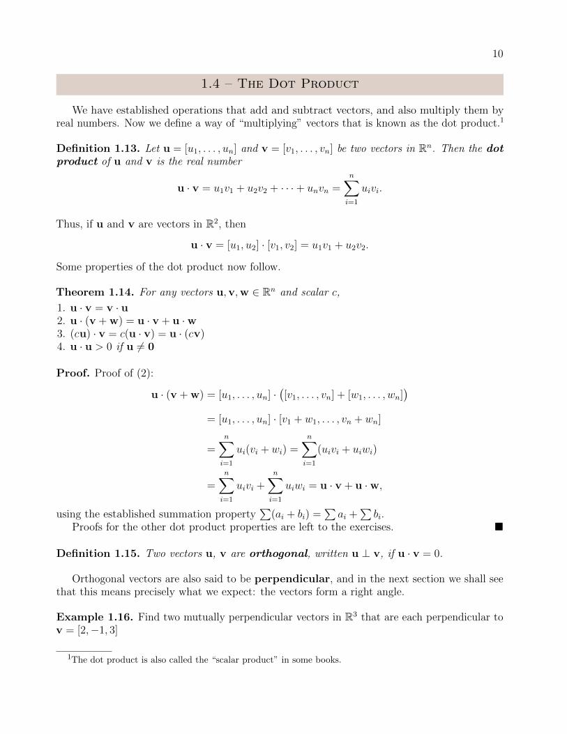
1.4 – The Dot Product

We have established operations that add and subtract vectors, and also multiply them byreal numbers. Now we define a way of “multiplying” vectors that is known as the dot product.1

Definition 1.13. Let u = [u1, . . . , un] and v = [v1, . . . , vn] be two vectors in Rn. Then the dotproduct of u and v is the real number

u · v = u1v1 + u2v2 + · · ·+ unvn =n∑i=1

uivi.

Thus, if u and v are vectors in R2, then

u · v = [u1, u2] · [v1, v2] = u1v1 + u2v2.

Some properties of the dot product now follow.

Theorem 1.14. For any vectors u,v,w ∈ Rn and scalar c,

1. u · v = v · u2. u · (v + w) = u · v + u ·w3. (cu) · v = c(u · v) = u · (cv)4. u · u > 0 if u 6= 0

Proof. Proof of (2):

u · (v + w) = [u1, . . . , un] ·([v1, . . . , vn] + [w1, . . . , wn]

)= [u1, . . . , un] · [v1 + w1, . . . , vn + wn]

=n∑i=1

ui(vi + wi) =n∑i=1

(uivi + uiwi)

=n∑i=1

uivi +n∑i=1

uiwi = u · v + u ·w,

using the established summation property∑

(ai + bi) =∑ai +

∑bi.

Proofs for the other dot product properties are left to the exercises. �

Definition 1.15. Two vectors u, v are orthogonal, written u ⊥ v, if u · v = 0.

Orthogonal vectors are also said to be perpendicular, and in the next section we shall seethat this means precisely what we expect: the vectors form a right angle.

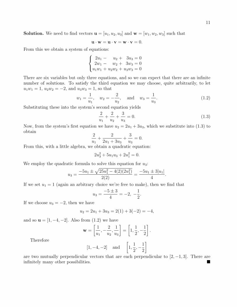
Example 1.16. Find two mutually perpendicular vectors in R3 that are each perpendicular tov = [2,−1, 3]

1The dot product is also called the “scalar product” in some books.

11

Solution. We need to find vectors u = [u1, u2, u3] and w = [w1, w2, w3] such that

u ·w = u · v = w · v = 0.

From this we obtain a system of equations: 2u1 − u2 + 3u3 = 02w1 − w2 + 3w3 = 0u1w1 + u2w2 + u3w3 = 0

There are six variables but only three equations, and so we can expect that there are an infinitenumber of solutions. To satisfy the third equation we may choose, quite arbitrarily, to letu1w1 = 1, u2w2 = −2, and u3w3 = 1, so that

w1 =1

u1, w2 = − 2

u2, and w3 =

1

u3. (1.2)

Substituting these into the system’s second equation yields

2

u1+

2

u2+

3

u3= 0. (1.3)

Now, from the system’s first equation we have u2 = 2u1 + 3u3, which we substitute into (1.3) toobtain

2

u1+

2

2u1 + 3u3+

3

u3= 0.

From this, with a little algebra, we obtain a quadratic equation:

2u23 + 5u1u3 + 2u21 = 0.

We employ the quadratic formula to solve this equation for u3:

u3 =−5u1 ±

√25u21 − 4(2)(2u21)

2(2)=−5u1 ± 3|u1|

4.

If we set u1 = 1 (again an arbitrary choice we’re free to make), then we find that

u3 =−5± 3

4= −2, −1

2.

If we choose u3 = −2, then we have

u2 = 2u1 + 3u3 = 2(1) + 3(−2) = −4,

and so u = [1,−4,−2]. Also from (1.2) we have

w =

[1

u1,− 2

u2,

1

u3

]=

[1,

1

2,−1

2

].

Therefore

[1,−4,−2] and

[1,

1

2,−1

2

]are two mutually perpendicular vectors that are each perpendicular to [2,−1, 3]. There areinfinitely many other possibilities. �

12

1.5 – The Norm of a Vector

Definition 1.17. The norm of a vector v ∈ Rn is ‖v‖ =√

v · v.

If v = [v1, . . . , vn], then

‖v‖ =√

[v1, . . . , vn] · [v1, . . . , vn] =

√∑n

i=1v2i (1.4)

The norm of a vector is also known as the vector’s magnitude or length. Consider alocated vector #„ov in the plane, which is a convenient representative of the vector v = [v1, v2].In §1.2 we saw that #„ov may be depicted as an arrow that starts at the origin o = (0, 0) andends at the point v = (v1, v2). How long is the arrow? The answer is given by the conventional(Euclidean) distance d(o, v) between o and v that is derived from the familiar PythagoreanTheorem:

d(o, v) =√

(v1 − 0)2 + (v2 − 0)2 =√v21 + v22.

On the other hand from (1.4) we have

‖v‖ =√v21 + v22,

and so ‖v‖ = d(o, v), the length of the arrow #„ov representing v. Note that if #„pq ∼ #„ov, wherep = (p1, p2) and q = (q1, q2), then

d(p, q) =√

(q1 − p1)2 + (q2 − p2)2 =√v21 + v22 = d(o, v) = ‖v‖

since q1 − p1 = v1 and q2 − p2 = v2, and so it does not matter which located vector we chooseto represent v: the length of the arrow will be the same! These truths stay true in R3 usingthe usual Euclidean conception of distance in three-dimensional space. In fact, in light of thefollowing definition they remain true in Rn for all n.

Definition 1.18. Let x,y ∈ Rn. The distance d(x,y), between x and y is given by

d(x,y) = ‖x− y‖.

Thus if x = [x1, . . . , xn] and y = [y1, . . . , yn], then

d(x,y) =

√∑n

i=1(xi − yi)2,

which reduces to the usual formula for the distance between points x and y when n equals 2 or3. That is, d(x,y) = d(x, y) in R2 or R3.

Remark. From now on we will frequently use the bold-faced symbol x for the vector [x1, . . . , xn]to represent the point x = (x1, . . . , xn). The logic of doing this is thus: a point x is naturallyidentified with its corresponding position vector # „ox, and # „ox is naturally identified with x. Such“vectorization” of points allows for a uniform notation in the statement of momentous resultsin vector calculus and the sciences. Moreover it places everything under consideration in thesetting of a “vector space,” which is the main object of study in linear algebra. So it must be

13

v

u

o

u

vc

x

o

u

vc v

Figure 6.

remembered: depending on context, x = [x1, . . . , xn] may be interpreted as a vector, a locatedvector, or a point!2

We are now in a position to justify Definition 1.15, by which we mean ground the definitionin more familiar geometric soil. Suppose u,v ∈ Rn are orthogonal vectors, which is to sayu · v = 0 and (since the dot product is commutative) v · u = 0. Recall that located vectorsrepresenting u, v and u + v may be chosen so that their corresponding arrows form a triangle,as at left in Figure 5. A triangle is a planar figure so it does not matter if the located vectorsare in an n-space for some n > 2: we can always orient the situation so that it lies on a plane.Now, ‖u + v‖ is the length of the longest side of the triangle, and ‖u‖ and ‖v‖ are the lengthsof the shorter sides. From the calculation

‖u + v‖2 =(√

(u + v) · (u + v))2

= (u + v) · (u + v)

= (u + v) · u + (u + v) · v = u · u + v · u + u · v + v · v= ‖u‖2 + ‖v‖2,

it can be seen that the lengths of the triangle’s sides obey the Pythagorean Theorem, and so itmust be that the triangle is a right triangle. That is, the sides formed by the located vectorsrepresenting u and v must meet at a right angle and therefore be perpendicular! It is in thissense that orthogonal vectors are also said to be “perpendicular.”

Proposition 1.19. If u,v ∈ Rn are orthogonal vectors, then ‖u + v‖2 = ‖u‖2 + ‖v‖2.

The proof has already been furnished above.

Definition 1.20. Let v 6= 0. The orthogonal projection of u onto v, projv u, is given by

projv u =(u · v

v · v

)v.

Once again it should help to ground the definition in geometry, because ultimately it isgeometry that motivates the definition. Let u,v ∈ Rn with v 6= 0. We represent these vectorsby located vectors with common initial point o as at left in Figure 6. For any c ∈ R let vc = cv.We wish to find the value for c so that the vector x represented by located vector # „vcu at rightin Figure 6 is orthogonal to v. This means c must be such that x · v = 0, and since vc + x = uwe obtain

(u− vc) · v = 0

2It was Henri Poincare who said “Mathematics is the art of giving the same name to different things.”

14

and thusu · v − vc · v = u · v − (cv) · v = 0.

Since (cv) · v = c(v · v) we finally arrive at

c =u · vv · v

. (1.5)

Now, consider the right side of Figure 6 again. It can be seen that the vector vc, as pictured,would be the shadow that u would cast upon v were a light to be directed upon the scenefrom directly overhead. It is in this sense that vc is a projection of u onto v—in particularthe orthogonal projection, since the “light rays” casting the “shadow” are perpendicular to v.Multiplying both sides of equation (1.5) by v gives

vc =(u · v

v · v

)v,

which is projv u as given in Definition 1.20.

Lemma 1.21. If u,v ∈ Rn, v 6= 0, and c is as in (1.5), then u− cv is orthogonal to v.

Proof. Taking the dot product,

(u− cv) · v = u · v − c(v · v) = u · v −(u · v

v · v

)(v · v) = u · v − u · v = 0,

we immediately conclude that u− cv ⊥ v. �

It’s a worthwhile exercise to verify that if u ⊥ v, then u ⊥ av for any scalar a. The lemmawill be used to prove the following.

Theorem 1.22 (Schwarz Inequality). If u,v ∈ Rn, then |u · v| ≤ ‖u‖‖v‖.

Proof. Suppose u,v ∈ Rn. If u = 0 or v = 0, then

|u · v| = |0| = 0 = ‖u‖‖v‖,

which affirms the theorem’s conclusion. So, suppose u,v 6= 0, and let c ∈ R be given by (1.5).Now,

(u− cv) · (cv) = c[(u− cv) · v] = c(0) = 0,

where (u− cv) · v = 0 by Lemma 1.21. Thus u− cv and cv are orthogonal, and by Proposition1.19

‖u‖2 = ‖(u− cv) + cv‖2 = ‖u− cv‖2 + ‖cv‖2.

Since ‖u− cv‖2 ≥ 0, this implies that ‖cv‖2 ≤ ‖u‖2. However,

‖cv‖2 = c2‖v‖2 =(u · v

v · v

)2(v · v) =

(u · v)2

v · v=

(u · v)2

‖v‖2,

and so from ‖cv‖2 ≤ ‖u‖2 we obtain

(u · v)2

‖v‖2≤ ‖u‖2,

whence comes (u ·v)2 ≤ ‖u‖2‖v‖2. Taking the square root of both sides completes the proof. �

15

From the Schwarz inequality we have

− ‖u‖‖v‖ ≤ u · v ≤ ‖u‖‖v‖,

and thus

−1 ≤ u · v‖u‖‖v‖

≤ 1

for any u,v 6= 0. This observation justifies the following definition.

Definition 1.23. Let u,v ∈ Rn be nonzero vectors. The angle between u and v is the numberθ ∈ [0, π] for which

cos θ =u · v‖u‖‖v‖

. (1.6)

Since the function cos : [0, π]→ [−1, 1] is one-to-one and onto, and the fraction in (1.6) onlytakes values in [−1, 1], there will always exist a unique value θ ∈ [0, π] that satisfies (1.6). FromDefinition 1.23 we have a new formula for the dot product:

u · v = ‖u‖‖v‖ cos θ. (1.7)

Some textbooks give this formula as the definition of the dot product, but it is less desirablesince the idea of a dot product is then founded on a geometric notion of angle that becomesproblematic to visualize in Rn for n > 3. However it is worthwhile verifying that the definitionof angle between vectors, as given here, agrees with our geometric intuition. For the sake ofsimplicity we can assume that u and v are nonzero vectors in R2, though the situation does notalter in Rn for n > 2 since two vectors can always be represented by coplanar located vectors.3

The approach will be to let θ be the geometric angle between u and v, and then show that (1.7)must necessarily follow.

Let 0 < θ < π. The vectors u, v, and u − v may be represented by located vectors thatform the triangle in Figure 7 (for convenience we depict θ as an acute angle).

By the Law of Cosines we obtain

‖u− v‖2 = ‖u‖2 + ‖v‖2 − 2‖u‖‖v‖ cos θ,

and since we’re assuming that u = [u1, u2] and v = [v1, v2], we obtain u− v = [u1 − v1, u2 − v2]so that

(u1 − v1)2 + (u2 − v2)2 = (u21 + u22) + (v21 + v22)− 2‖u‖‖v‖ cos θ,

3This is because two located vectors can be defined by three points p, q, and r, such as #„pq and #„pr, and threepoints define a plane.

u

u− v

vθ

Figure 7.

16

and hence

‖u‖‖v‖ cos θ = u1v1 + u2v2 = u · v.

In the cases when θ = 0 or θ = π we find that v = ku = [ku1, ku2] for some nonzero scalark; that is, u and v are parallel vectors, and we have

‖u‖‖v‖ cos θ = ‖u‖‖ku‖ cos θ = |k|(u21 + u22) cos θ. (1.8)

If θ = 0, then k > 0 so that |k| = k and cos θ = 1; and if θ = π, then k < 0 so that |k| = −kand cos θ = −1. In either case, from (1.8) we obtain

‖u‖‖v‖ cos θ = k(u21 + u22) = [u1, u2] · [ku1, ku2] = u · v

as desired.

Example 1.24. Let u = [2,−1, 5] and v = [−1, 1, 1].

(a) Find ‖u‖ and ‖v‖.(b) Find projv u, the orthogonal projection of u onto v.(c) Find proju v, the orthogonal projection of v onto u.(d) Find the angle between u and v to the nearest tenth of a degree.

Solution.

(a) We have

‖u‖ =√

22 + (−1)2 + 52 =√

30 and ‖v‖ =√

(−1)2 + 12 + 12 =√

3.

(b) Since

u · v = (2)(−1) + (−1)(1) + (5)(1) = 2 and v · v = ‖v‖2 = (√

3)2 = 3,

we have

projv u =(u · v

v · v

)v =

2

3[−1, 1, 1] =

[−2

3,2

3,2

3

].

(c) Since

v · u = u · v = 2 and u · u = ‖u‖2 = (√

30)2 = 30,

we have

proju v =(v · u

u · u

)u =

2

30[2,−1, 5] =

[2

15,− 1

15,1

3

].

(d) By definition,


=2√

30√

3=

2

3√

10,

and thus

θ = cos−1(

2

3√

10

)≈ 77.8◦.

�

17

θ θ

Figure 8.

Example 1.25. Find the measure of the angle θ between the diagonal of a cube and thediagonal of one of its faces, as shown in Figure 8.

Solution. It will be convenient to regard the cube as existing in R3, with edges of length 1,and the vertex where the two diagonals meet situated at the origin (0, 0, 0). We can then setup coordinate axes such that the cube diagonal has endpoints (0, 0, 0) and (1, 1, 1), and theface diagonal has endpoints (0, 0, 0) and (0, 1, 1). Thus the diagonals can be characterized aspositions vectors u = [1, 1, 1] and v = [0, 1, 1]. Now,


=[1, 1, 1] · [0, 1, 1]√

12 + 12 + 12√

02 + 12 + 12=

2√6,

and so

θ = cos−1(

2√6

)≈ 35.264◦

is the angle’s measure. �

Problems

1. Find the measure of the angle θ between the diagonal of a cube and one of its edges, asshown below.

θ

18

1.6 – Lines and Planes

In R2 a line L is typically defined to be the solution set to an equation of the form ax+by = cfor constants a, b, c ∈ R, where a and b are not both zero. That is, L is the set of points

{(x, y) : ax+ by = C},

and ax+ by = C is called the Cartesian equation (or algebraic equation) for L. In Rn forn > 2 we can still speak geometrically of lines, of course, but it becomes impossible to define theline using a single Cartesian equation. The most convenient remedy for this is to use vectors,thereby motivating the following definition.

Definition 1.26. Let p,v ∈ Rn with v 6= 0. The line through p and parallel to v ∈ Rn is theset of vectors of the form

{p + tv : t ∈ R}.

A parametric equation (or parametrization) of a line L = {p + tv : t ∈ R} ⊆ Rn is anyvector-valued function x : R→ Rn given by

x(t) = p + tv

for some p ∈ L and vector v parallel to v. (Here t is called a parameter.) Thus we find that

x(t) = p + tv

is one parametrization for L, but there are infinitely many others in existence.Given a parametrization x(t) = p + tv for some line in Rn, the vector p = [p1, . . . , pn] may

more naturally be thought of as the position vector #„op of the point p = (p1, . . . , pn), and so ineveryday speech p may be referred to as a point even though mathematically it is handled as avector. The same applies to the vector

x(t) = [x1(t), . . . , xn(t)]

for each t ∈ R: we may regard it, if desired, as the position vector of the point

x(t) = (x1(t), . . . , xn(t)),

and so refer to it as a point. In contrast, for each t ∈ R the vector tv may be thought of as alocalized vector (i.e. an arrow) with initial point at p and terminal point located at anotherpoint on the line.

Definition 1.27. The line segment in Rn with endpoints p,q ∈ Rn is the set of vectors ofthe form

{p + t(q− p) : t ∈ [0, 1]}.

A natural parametrization for a line segment with endpoints p and q is the vector-valuedfunction x : [0, 1]→ Rn given by

x(t) = p + t(q− p), (1.9)

19

though it is frequently the case in applications that other parametrizations may be considered.In (1.9) we have x(0) = p and x(1) = q, and so as t increases from 0 to 1 we see that we “travel”along the line segment from p to q. However, the alternative parametrization

x(t) = q + t(p− q)

reverses the direction of travel.

Example 1.28. Find a parametrization x(t) of the line containing the points p = (2,−6, 9)and q = (0, 8, 1), such that x(1) = p and x(−2) = q.

Solution. We must have x(t) = p + f(t)(q− p) for some function f such that f(1) = 0 andf(−2) = 1. The simplest such function is a linear one, which is to say f(t) = mt+b for constantsm and b. With the condition f(1) = 0 we obtain b = −m, so that f(t) = m(t− 1). With thecondition f(−2) = 1 we obtain 1 = m(−2− 1), or m = −1/3, and hence b = 1/3. Now we have

x(t) = p +(− 1

3t+ 1

3

)(q− p)

for p = [2,−6, 9] and q = [0, 8, 1], giving

x(t) =[43,−4

3, 19

3

]+ t[23,−14

3, 83

].

Other answers are possible if we choose f to be a nonlinear function. �

In R3 a line P is sometimes defined to be the solution set to an equation of the formax+ by + cz = d for constants a, b, c, d ∈ R, where a, b, c are not all zero. That is, P is the setof points

{(x, y, z) : ax+ by + cz = d},

where ax+ by + cz = d is the Cartesian equation for P . In Rn for n > 3 we may still wishto conceive of planes, but it is no longer possible to define the plane using a single Cartesianequation. The following definition uses vectors to define the notion of a plane for all Rn withn ≥ 3.

Definition 1.29. Let u,v ∈ Rn be nonzero, nonparallel vectors. The plane through pointp ∈ Rn and parallel to u,v is the set of vectors of the form

{p + su + tv : s, t ∈ R}.

A parametric equation (or parametrization) of a plane P = {p+su+ tv : t ∈ R} ⊆ Rn

is any vector-valued function x : R2 → Rn given by

x(s, t) = p + su + tv

for some p ∈ P and vectors u and v parallel to u and v, respectively. (Here and s and t arecalled the parameters.) Thus

x(s, t) = p + su + tv (1.10)

is one parametrization for P among infinitely many.A normal vector for a plane P having parametrization (1.10) is a nonzero vector n such

that n · u = 0 and n · v = 0. A line L is said to be orthogonal to P if L is parallel to n. If L

20

is orthogonal to P and p ∈ L∩ P (i.e. p is the point of intersection between L and P ), then thedistance between any point q ∈ L and P is the length of the line segment pq.

Example 1.30. Find both a parametric and Cartesian equation for the plane P containing thepoint (0, 0, 0) that is orthogonal to the line L having parametric equation

x(t) = [3,−2, 1] + t[2, 1,−3].

Solution. By definition any normal vector n for P must be parallel to L, which in turn meansthat n must be parallel to a direction vector of L. Since [2, 1,−3] is an obvious direction vectorof L, we may let n = [2, 1,−3]. Geometrically speaking, since P contains the point o = (0, 0, 0),P will consist precisely of those points (x, y, z) for which the vector [x, y, z]− [0, 0, 0] = [x, y, z]is orthogonal to n. Since

n · [x, y, z] = 0 ⇔ [2, 1,−3] · [x, y, z] = 0 ⇔ 2x+ y − 3z = 0,

we conclude that 2x+ y − 3z = 0 is a Cartesian equation for P .To find a parametric equation, we use the Cartesian equation to find two other points on P

besides (0, 0, 0), such as p = (1,−2, 0) and q = (0, 3, 1). Now let

u = p− 0 = [1,−2, 0] and v = q− 0 = [0, 3, 1].

A parametric equation for P is x(s, t) = 0 + su + tv, or

x(s, t) = s[1,−2, 0] + t[0, 3, 1]

for s, t ∈ R. �

Example 1.31. Find a normal vector for the plane 3x+ 2y − 2z = 3.

Solution. We first find three points on the plane that are not collinear. This can be done bysubstituting values for x and y in the equation, say, and then solving for z. In this way we findpoints (0, 0, 1/7), (1, 1, 1), and (1, 2, 2).

Example 1.32. Find the distance between the point q = (1,−2, 4) and the plane 3x+2y−2z = 3.

Solution. Letting x = y = 0 in the plane’s equation gives z = 1/7, so p = (0, 0, 1/7) is a pointon the plane. Let

v = #„pq = q− p =[5, 2,−22

7

].

A normal vector for the plane is n = [4,−4, 7]. We project v onto n:

projn(v) =(v · n

n · n

)n = −10

81[4,−4, 7].

The magnitude of this vector,D = ‖ projn(v)‖ = 10

9,

is the sought-after distance. �

21

Problems

1. Let L1 be the line given by x(t) = [1, 1, 1] + t[2, 1,−1], and let L2 be the line with Cartesianequations

x = 5, y − 4 =z − 1

2.

(a) Show that the lines L1 and L2 intersect, and find the point of intersection.(b) Find a Cartesian equation of the plane containing L1 and L2.

2. Let P be the plane in R3 which has normal vector n = [1,−4, 2] and contains the pointa = (5, 1, 3).

(a) Find a Cartesian equation for P .(b) Find a parametric equation for P .

22

2Matrices and Systems

2.1 – Matrices

Let m,n ∈ N, and let F be a field. An m× n matrix over F is a rectangular array ofelements of F arranged in m rows and n columns:

a11 a12 · · · a1na21 a22 · · · a2n...

.... . .

...am1 am2 · · · amn

. (2.1)

The values m and n are called the dimensions of the matrix. The scalar (i.e. element ofF) in the ith row and jth column of the matrix, aij, is known as the ij-entry. To be clear,throughout these notes the entries aij of a matrix are always taken to be elements of some fieldF, which could be the real number system R, the complex number system C, or some other field.

A 1× 1 matrix [a] is usually identified with the scalar a ∈ F that constitutes its sole entry.For n ≥ 2, both n× 1 and 1× n matrices are called vector matrices (or simply vectors). Inparticular an n× 1 matrix

x1x2...xn

(2.2)

is a column vector (or column matrix), and a 1× n matrix[x1 x2 · · · xn

]is a row vector (or row matrix). Henceforth the Euclidean vector [x1, . . . , xn] introduced inChapter 1 will most of the time be represented by its corresponding column vector (2.2) so asto take advantage of the convenient properties of matrix arithmetic.

The matrix (2.1) we typically denote more compactly by the symbol

[aij]m,n,

23

which indicates that the ij-entry is the scalar aij, where i ∈ {1, . . . ,m} is the row number andj ∈ {1, . . . , n} is the column number. We call the sets {1, . . . ,m} and {1, . . . , n} the range ofthe indexes i and j, respectively. If m = n then a square matrix results, and we define

[aij]n = [aij]n,n.

(Care should be taken with this notation: [aij ]m,n denotes an m×n matrix, while [aij ]mn denotesan mn×mn square matrix!) If the range of the indexes i and j are known or irrelevant, we willwrite (2.1) as simply [aij]. Another word about square matrices: The diagonal entries of asquare matrix [aij]n are the entries with matching row and column number: a11, . . . , ann.

Very often we have no need to make any reference to the entries of a matrix, in which casewe will usually designate the matrix by a bold-faced upper-case letter such as A, B, C, and soon. The exception is vector matrices, which are normally labeled with bold-faced lower-caseletters such as a, b, x, y and so on. If we need to make reference to the ij-entry of a matrix A,then the symbol [A]ij stands ready to denote it. Thus if A = [aij]m,n, then

[A]ij = aij.

The set of all m× n matrices with entries in the field F will be denoted by Fm×n. That is,

Fm×n ={

[aij]m,n : aij ∈ F for all 1 ≤ i ≤ m, 1 ≤ j ≤ n}.

From this point onward we also define

Fn = Fn×1

in these notes; that is, Fn is the set of matrices consisting of n entries from F arranged in asingle column. The exception has already been encountered: throughout the first chapter (andonly the first chapter) we always took Rn to signify R1×n. In the wider world of mathematicsbeyond these notes the symbol Fn denotes either row vectors (elements of F1×n) or columnvectors (elements of Fn×1), depending on an author’s whim.

If aij = 0 for all 1 ≤ i ≤ m and 1 ≤ j ≤ n, then we obtain the m× n zero matrix

Om,n = [0]m,n =

0 0 · · · 00 0 · · · 0...

.... . .

...0 0 · · · 0

having m rows and n columns of zeros. In particular we define

On = On,n.

In any case the symbol O will always denote a zero matrix of some kind, whereas 0 will continueto denote more specifically a zero vector (i.e. a row or column matrix consisting of zeros).

Definition 2.1. If A,B ∈ Fm×n and c ∈ F, then we define sum A + B and scalar multiplecA to be the matrices in Fm×n with ij-entry

[A + B]ij = [A]ij + [B]ij and [cA]ij = c[A]ij

for all 1 ≤ i ≤ m and 1 ≤ j ≤ n.

24

Put another way, letting A = [aij] and B = [bij], we have

A + B = [aij + bij] =

a11 + b11 a12 + b12 · · · a1n + b1na21 + b21 a22 + b22 · · · a2n + b2n

......

. . ....

am1 + bm1 am2 + bm2 · · · amn + bmn

and

cA = [caij] =

ca11 ca12 · · · ca1nca21 ca22 · · · ca2n

......

. . ....

cam1 cam2 · · · camn

.Thus matrix addition and matrix scalar multiplications is analogous to the addition and scalarmultiplication of Euclidean vectors. Clearly matrix addition is commutative, which is to say

A + B = B + A

for any A,B ∈ Fm×n. We define the additive inverse of A to be the matrix −A given by

−A = (−1)A = [−aij].

That

A + (−A) = −A + A = O

is straightforward to check.

Definition 2.2. Let A ∈ Fm×n. The transpose of A is the matrix A> ∈ Fn×m such that

[A>]ij = [A]ji

for all 1 ≤ i ≤ n and 1 ≤ j ≤ m.

Put another way, if A = [aij]m,n, then the transpose of A is the matrix A> = [αji]n,m withαji = aij for each 1 ≤ j ≤ n, 1 ≤ i ≤ m. Thus the number aij in the ith row and jth column ofA is in the jth row and ith column of A>, so that

A> =

a11 a21 · · · am1

a12 a22 · · · am2...

.... . .

...a1n a2n · · · amn

. (2.3)

Comparing (2.3) with (2.1), it can be seen that the rows of A simply become the columns ofA>. For example if

A =

[−3 7 4

6 −5 10

],

then

A> =

−3 67 −54 10

.

25

It is easy to see that (A>)> = A. We say A is symmetric if A> = A, and skew-symmetric if A> = −A. The set of all symmetric n× n matrices with entries in the field Fwill be denoted by Symn(F); that is,

Symn(F) ={A ∈ Fn×n : A> = A

}.

The symbol Skwn(F) will denote the set of all skew-symmetric n× n matrices with entries in F:

Skwn(F) ={A ∈ Fn×n : A> = −A

}.

A standard approach to proving that two matrices A and B are equal is to first confirm thatthey have the same dimensions, and then show that the ij-entry of the matrices are equal forany i and j. Thus we verify that A and B are m× n matrices (a step that may be omitted if itis clear), then verify that [A]ij = [B]ij for arbitrary 1 ≤ i ≤ m and 1 ≤ j ≤ n. The proof of thefollowing proposition illustrates the method.

Proposition 2.3. Let A,B ∈ Fm×n, and let c ∈ F. Then

1. (cA)> = cA>

2. (A + B)> = A> + B>

3. (A>)> = A.

Proof.Proof of Part (1). Fix 1 ≤ i ≤ m and 1 ≤ j ≤ n. Then, applying Definitions 2.1 and 2.2,

[(cA)>]ij = [cA]ji = c[A]ji = c[A>]ij = [cA>]ij.

So we see that the ij-entry of (cA)> equals the ij-entry of cA>, and since i and j were arbitrary,it follows that (cA)> = cA>.

Proof of Part (2). We have

[(A + B)>]ij = [A + B]ji = [A]ji + [B]ji = [A>]ij + [B>]ij = [A> + B>]ij,

so the ij-entries of (A + B)> and A> + B> are equal. �

The proof of part (3) of Proposition 2.3, which can be done using the same “entrywise”technique, is left as a problem.

The trace of a square matrix A = [aij]n,n, written tr(A), is the sum of the diagonal entriesof A:

tr(A) =n∑i=1

aii. (2.4)

Since A> = [αij]n,n such that αij = aji, we readily obtain

tr(A>) =n∑i=1

αii =n∑i=1

aii = tr(A).

Other properties of the trace and transpose operations will be established in future sections.A block matrix is a matrix whose entries are themselves matrices. The matrices that

constitute a block matrix are called submatrices. In practice a block matrix is typically

26

constructed from an ordinary matrix A ∈ Fm×n by partitioning the entries into two or moresmaller arrays with the placement of vertical or horizontal rules, such as

a11 · · · a1s a1,s+1 · · · a1n...

. . ....

.... . .

...ar1 · · · ars ar,s+1 · · · arn

ar+1,1 · · · ar+1,s ar+1,s+1 · · · ar+1,n...

. . ....

.... . .

...am1 · · · ams am,s+1 · · · amn

, (2.5)

which partitions the matrix A = [aij]m,n into four submatricesa11 · · · a1s...

. . ....

ar1 · · · ars

,a1,s+1 · · · a1n

.... . .

...ar,s+1 · · · arn

,ar+1,1 · · · ar+1,s

.... . .

...am1 · · · ams

,ar+1,s+1 · · · ar+1,n

.... . .

...am,s+1 · · · amn

,where of course 1 ≤ r < m and 1 ≤ s < n. If we designate the above submatrices as A1, A2,A3, and A4, respectively, then we may write (2.5) as the block matrix[

A1 A2

A3 A4

]or

[A1 A2

A3 A4

],

with the latter representation being preferred in these notes except in certain situations. Ablock matrix is also known as a partitioned matrix.

Problems

1. Prove that (A>)> = A for any A ∈ Fm×n.

2. Prove that (A + B + C)> = A> + B> + C> for any A,B,C ∈ Fm×n.

3. Prove that (aA + bB)> = aA> + bB> for any A,B ∈ Fm×n and a, b ∈ F.

27

2.2 – Matrix Multiplication

The definition of the product of two matrices is relatively more involved than that foraddition or scalar multiplication.

Definition 2.4. Let A ∈ Fm×n and B ∈ Fn×p. Then the product of A and B is the matrixAB ∈ Fm×p with ij-entry given by

[AB]ij =n∑k=1

[A]ik[B]kj

for 1 ≤ i ≤ m and 1 ≤ j ≤ p.

Letting A = [aij]m,n and B = [bij]n,p, it is immediate that AB = [cij]m,p with ij-entry

cij =n∑k=1

aikbkj.

That is,

AB = [aij]m,n[bij]n,p =[∑n

k=1aikbkj

]m,p

, (2.6)

where it’s understood that 1 ≤ i ≤ m is the row number and 1 ≤ j ≤ p is the column numberof the entry

∑nk=1 aikbkj.

Example 2.5. If

A =

[−3 0 6

2 11 −5

]and B =

4 9 −60 −1 2−4 0 −3

,so that A is a 2× 3 matrix and B is a 3× 3 matrix, then AB is a 2× 3 matrix given by

AB =

[−3 0 6

2 11 −5

] 4 9 −60 −1 2−4 0 −3

=

[−3 0 6

] 40−4

[−3 0 6

] 9−1

0

[−3 0 6

]−62−3

[2 11 −5

] 40−4

[2 11 −5] 9−1

0

[2 11 −5]−6

2−3

=

[−36 −27 0

28 7 25

].

The product BA is undefined. �

28

Vectors may be used to better see how the product AB is formed. Let

ai =[ai1 · · · ain

]denote the row vectors of A for 1 ≤ i ≤ m,

a1→ a11 a12 · · · a1na2→ a21 a22 · · · a2n...

......

. . ....

am→ am1 am2 · · · amn

= A (2.7)

and let

bj =

b1j...bnj

denote the column vectors of B for 1 ≤ j ≤ p,

B =

b1 b2 · · · bp↓ ↓ ↓

b11 b12 · · · b1pb21 b22 · · · b2p...

.... . .

...bn1 bn2 · · · bnp

. (2.8)

Then by definition

AB = [aibj]m,p =

a1b1 a1b2 · · · a1bpa2b1 a2b2 · · · a2bp

......

. . ....

amb1 amb2 · · · ambp

,which makes clear that the ij-entry is

[AB]ij = aibj =[[[ai1 · · · ain

]]]b1j...bnj

= ai1b1j + ai2b2j + · · ·+ ainbnj =n∑k=1

aikbkj,

in agreement with Definition 2.4. Note that AB is not defined if the number of columns in A isnot equal to the number of rows in B!

It is common—and convenient—to denote matrices (2.7) and (2.8) by the symbolsa1

a2...

am

and[b1 b2 · · · bp

],

respectively, and so we have

AB =

a1

a2...

am

[b1 b2 · · · bp]=

a1b1 a1b2 · · · a1bpa2b1 a2b2 · · · a2bp

......

. . ....

amb1 amb2 · · · ambp

. (2.9)

29

For any j = 1, . . . , p we have bj ∈ Fn, which is to say bj has n rows and so Abj can be computedfollowing the pattern of (2.9):

Abj =

a1

a2...

am

bj =

a1bja2bj

...ambj

.(This can be verified easily by working directly with Definition 2.4.) Comparing this result withthe right-hand side of (2.9), we see that Abj is the jth column vector of AB; that is, we havethe following.

Proposition 2.6. If A ∈ Fm×n and B = [ b1 · · · bp ] ∈ Fn×p, then

AB = A[b1 · · · bp

]=[Ab1 · · · Abp

].

We see how a judicious use of notation can reap significant labor-saving rewards, leadingfrom the unfamiliar characterization of AB given in Definition 2.4 to the perfectly naturalformula in Proposition 2.6.

Theorem 2.7. Let A ∈ Fm×n, B,C ∈ Fn×p, D ∈ Fp×q, and c ∈ F. Then

1. A(cB) = c(AB).2. A(B + C) = AB + AC (the distributive property).3. (AB)D = A(BD) (the associative property).

Proof.Proof of Part (1). Clearly A(cB) and c(AB) are both m× p matrices. Now, for any 1 ≤ i ≤ mand 1 ≤ j ≤ p,

[A(cB)]ij =n∑k=1

[A]ik[cB]kj Definition 2.4

=n∑k=1

[A]ik(c[B]kj

)Definition 2.1

= c

n∑k=1

[A]ik[B]kj Definition 1.5(F5,6,7)

= c[AB]ij Definition 2.4,

= [c(AB)]ij Definition 2.1,

and so we see the ij-entries of A(cB) and c(AB) are equal.

Proof of Part (2). Clearly A(B + C) and AB + AC are both m× p matrices. For 1 ≤ i ≤ mand 1 ≤ j ≤ p,

[A(B + C)]ij =n∑k=1

[A]ik[B + C]kj Definition 2.4

30

=n∑k=1

[A]ik([B]kj + [C]kj

)Definition 2.1

=n∑k=1

[A]ik[B]kj +n∑k=1

[A]ik[C]kj Definition 1.5(F6)

= AB + AC. Definition 2.4,

which shows equality of the ij entries.

Proof of Part (3). Both matrices will be m×q. Using basic summation properties and Definition2.4,

[(AB)D]ij =

p∑k=1

[AB]ik[D]kj =

p∑k=1

[(n∑`=1

[A]i`[B]`k

)[D]kj

]=

n∑`=1

p∑k=1

[A]i`[B]`k[D]kj

=n∑`=1

([A]i`

p∑k=1

[B]`k[D]kj

)=

n∑`=1

[A]i`[BD]`j = [A(BD)]ij,

and the proof is done. �

In light of the associative property of matrix multiplication it is not considered ambiguous towrite ABD, since whether we interpret it as meaning (AB)D or A(BD) makes no difference.The order of operations conventions dictate that ABD be computed in the order indicated by(AB)D, however.

Proposition 2.8. If A ∈ Fm×n, B ∈ Fn×p, C ∈ Fp×q, and D ∈ Fq×r, then

(AB)(CD) = A(BC)D.

Proof. Let AB = P. We have

(AB)(CD) = P(CD) = (PC)D = [(AB)C]D = [A(BC)]D, (2.10)

where the second and fourth equalities follow from Theorem 2.7(3). Next we obtain

[A(BC)]D = A(BC)D, (2.11)

since the order of operations in evaluating either expression is precisely the same: (1) execute Btimes C to obtain BC; (2) execute A times BC to obtain A(BC); (3) execute A(BC) timesD to obtain A(BC)D.

Combining (2.10) and (2.11) yields (AB)(CD) = A(BC)D. �

There is no useful way to divide matrices, but we can easily define what it means toexponentiate a matrix by a positive integer.

31

Definition 2.9. If A ∈ Fn×n and m ∈ N, then

Am = AA · · ·A︸︷︷︸m factors

=m∏k=1

A.

In particular A1 = A.

The definition makes use of so-called product notation,m∏k=1

xk = x1x2x3 · · ·xm,

which does for products what summation notation does for sums.The Kronecker delta is a function δij : Z×Z→ {0, 1} defined as follows for integers i and

j:

δij =

{1, if i = j

0, if i 6= j

We use the Kronecker delta to define the n× n identity matrix,

In = [δij]n =

1 0 · · · 00 1 · · · 0...

.... . .

...0 0 · · · 1

,the n× n matrix with diagonal entries 1 and all other entries 0. In particular we have

I2 =

[1 00 1

]and I3 =

1 0 00 1 00 0 1

Definition 2.10. For any A ∈ Fn×n we define A0 = In.

If the dimensions of an identity matrix are known or irrelevant, then the abbreviated symbolI may be used. The reason In is called the identity matrix is because, for any n× n matrix A,it happens that

InA = AIn = A.

Thus In acts as an identity with respect to matrix multiplication, just as 1 is the identity withrespect to multiplication of real numbers. In fact it can be shown that In is the identity formatrix multiplication, as there can be no others.

Example 2.11. Show that I2 is the only matrix for which I2A = AI2 = A holds for all 2× 2matrices A.

Solution. Given any 2× 2 matrix

A =

[a11 a12a21 a22

],

32

we have

AI2 =

[a11 a12a21 a22

][1 00 1

]=

[a11(1) + a12(0) a11(0) + a12(1)a21(1) + a22(0) a21(0) + a22(1)

]=

[a11 a12a21 a22

]= A

and

I2A =

[1 00 1

][a11 a12a21 a22

]=

[(1)a11 + (0)a12 (0)a11 + (1)a12(1)a21 + (0)a22 (0)a21 + (1)a22

]=

[a11 a12a21 a22

]= A,

so certainly I2A = AI2 = A holds for all A.Now, let B be a 2× 2 matrix such that

BA = AB = A (2.12)

for all 2× 2 matrices A. If we set A = I2 in (2.12) we obtain BI2 = I2 in particular, whenceB = I2. Therefore I2 is the only matrix for which I2A = AI2 = A holds for all A. �

To show more generally that In is the only matrix for which

InA = AIn = A

for all A ∈ Fn×n involves a nearly identical argument.

Proposition 2.12. Let A ∈ Fn×n.

1. If Ax = x for every n× 1 column vector x, then A = In.2. If Ax = 0 for every n× 1 column vector x, then A = On.

Proof.Proof of Part (1). Suppose that Ax = x for all n× 1 column vectors x. For each 1 ≤ j ≤ n let

ej = [δij]n,1 =

δ1j...δnj

,where once again we make use of the Kronecker delta. Thus ej is the n× 1 column vector with1 in the jth row and 0 in all other rows.

Now, for each 1 ≤ j ≤ n, Aej is an n× 1 column vector with i1-entry equalling

n∑k=1

aikδkj = aijδjj = aij.

for each 1 ≤ i ≤ n. On the other hand Aej = ej by hypothesis, and so

aij = δij =

{0, if i 6= j

1, if i = j

for all 1 ≤ i, j ≤ n. But this is precisely the definition for In, and therefore A = In. �

33

The proof of part (2) of the proposition is similar and left as a problem. Observe that, inthe notation established in the proof of part (1), we have

In =[

[δi1]n,1 · · · [δin]n,1

]=[e1 · · · en

]. (2.13)

Proposition 2.13. Let A ∈ Fm×n and B ∈ Fn×p. Then

(AB)> = B>A>.

Proof. Note that B> is p× n and A> is n×m, so the product B>A> is defined as a p×mmatrix. Fix 1 ≤ i ≤ p and 1 ≤ j ≤ m. We have, using Definition 2.4 and Definition 2.2 twiceeach,

[B>A>]ij =n∑k=1

[B>]ik[A>]kj =

n∑k=1

[B]ki[A]jk =n∑k=1

[A]jk[B]ki = [AB]ji =[(AB)>

]ij.

Thus the ij-entry of B>A> is equal to the ij-entry of (AB)>, so B>A> = (AB)> as was to beshown. �

Problems

1. Given that

x =

3−1

2

, A =

1 2 −33 0 −1−2 1 4

, C =

−4 21 −10 3

compute the following.

(a) x>x

(b) xx>

(c) AC

34

2.3 – Elementary Row and Column Operations

We start by establishing some necessary notation. The symbol En,lm will denote the n× nmatrix with lm-entry 1 and all other entries 0; that is,

En,lm = [δilδmj]n

for any fixed 1 ≤ l,m ≤ n, making use of the Kronecker delta introduced in the last section.Put yet another way, En,lm is the n× n matrix with ij-entry δilδmj:

[En,lm]ij = δilδmj. (2.14)

Usually the n in the symbol En,lm may be suppressed without leading to ambiguity, so thatthe more compact symbol Elm may be used. This will usually be done except in the statementof theorems.

Proposition 2.14. Let n ∈ N and 1 ≤ l,m, p, q ≤ n.

1. En,lmEn,mp = En,lp.2. If m 6= p, then En,lmEn,pq = On.

Proof.Proof of Part (1). Using Definition 2.4 and equation (2.14), the ij-entry of ElmEmp is

[ElmEmp]ij =n∑k=1

[Elm]ik[Emp]kj =n∑k=1

(δilδmk)(δkmδpj) = (δilδmm)(δmmδpj) = δilδpj,

where the third equality is justified since δmk = 0 for all k 6= m, and then we need only recallthat δmm = 1. So ElmEmp is the n× n matrix with ij-entry δilδpj , and therefore ElmEmp = Elp.

Proof of Part (2). Suppose m 6= p. Again using Definition 2.4 and equation (2.14), the ij-entryof ElmEmp is

[ElmEpq]ij =n∑k=1

[Elm]ik[Epq]kj =n∑k=1

(δilδmk)(δkpδqj) = 0,

where the third equality is justified since, for any 1 ≤ k ≤ n, either k 6= m or k 6= p, and soeither δmk = 0 or δkp = 0. Therefore ElmEpq = On. �

Let n ∈ N. For any scalar c 6= 0 define

Mi(c) = In + (c− 1)Eii,

which is the n× n matrix obtained by multiplying the ith row of In by c. Also define

Mi,j = In − Eii − Ejj + Eij + Eji

for i, j ∈ {1, . . . , n} with i 6= j, which is the matrix obtained by interchanging the ith and jthrows of In (notice that Mi,j = Mj,i). Finally, for i, j ∈ {1, . . . , n} with i 6= j, and scalar c 6= 0,define

Mi,j(c) = In + cEji,

35

which is the matrix obtained by adding c times the ith row of In to the jth row of In. Anymatrix of the form Mi,j(c), Mi,j, or Mi(c) is called an elementary matrix.

Definition 2.15. Given A ∈ Fm×n, an elementary row operation on A is any one of themultiplications

Mi,j(c)A, Mi,jA, Mi(c)A.

More specifically we call left-multiplication by Mi,j(c) an R1 operation, left-multiplication byMi,j an R2 operation, and left-multiplication by Mi(c)A an R3 operation. A matrix A′ is calledrow-equivalent to A if there exist elementary matrices M1, . . . ,Mk such that

A′ = Mk · · ·M1A.

An elementary column operation on A is any one of the multiplications

AM>i,j(c), AM>

i,j, or AM>i (c).

More specifically we call right-multiplication by M>i,j(c) a C1 operation, right-multiplication by

M>i,j a C2 operation, and right-multiplication by M>

i (c) a C3 operation. A matrix A′ is calledcolumn-equivalent to A if there exist elementary matrices M1, . . . ,Mk such that

A′ = AM>1 · · ·M>

k .

It’s understood that the elementary matrices in the first part of Definition 2.15 must all bem×m matrices, and the elementary matrices in the second part must be n× n. Also, to beclear, we define M>

i,j(c) = [Mi,j(c)]> and M>

i (c) = [Mi(c)]>. Finally, we define any matrix A

to be both row-equivalent and column-equivalent to itself.When we need to denote a collection of, say, p elementary matrices in a general way, we will

usually use symbols M1, . . . ,Mp. So for each k = 1, . . . , p the symbol Mk could represent anyone of the three basic types of elementary matrix given in Definition 2.15.

Proposition 2.16. Suppose A ∈ Fm×n has row vectors a1, . . . , am ∈ Fn. Let c 6= 0, and let1 ≤ p, q ≤ m with p 6= q.

1. Mp,q(c)A is the matrix obtained from A by replacing the row vector aq by aq + cap:

Mp,q(c)

...

aq...

=

...

aq + cap...

.2. Mp,qA is the matrix obtained from A by interchanging ap and aq:

Mp,q

...

amin{p,q}...

amax{p,q}...

=

...

amax{p,q}...

amin{p,q}...

.

36

3. Mp(c)A is the matrix obtained from A by replacing ap by cap:

Mp(c)

...

ap...

=

...cap

...

.Proof.Proof of Part (1). Fix 1 ≤ i ≤ m and 1 ≤ j ≤ n. Here Mp,q(c) must be m × m, so thatMp,q(c) = Im + cEm,qp, since A is m× n. Then[

Mp,q(c)A]ij

=m∑k=1

[Mp,q(c)

]ik

[A]kj =m∑k=1

[Im + cEqp]ik[A]kj

=m∑k=1

([Im]ik + c[Eqp]ik

)[A]kj =

m∑k=1

[Im]ik[A]kj + c

m∑k=1

[Eqp]ik[A]kj

= [ImA]ij + cm∑k=1

δiqδpk[A]kj = [A]ij + cδiq[A]pj,

where the last equality holds since δpk = 0 for all k 6= p.Now, if i 6= q, then δiq = 0 and we obtain[

Mp,q(c)A]ij

= [A]ij

for all 1 ≤ j ≤ n, which shows that the ith row vector of Mp,q(c)A equals the ith row vector aiof A whenever i 6= q. On the other hand if i = q, then δiq = δqq = 1 and we obtain[

Mp,q(c)A]qj

= [A]qj + c[A]pj

for all 1 ≤ j ≤ n, which shows that the qth row vector of Mp,q(c)A equals the qth row vector ofA plus c times the pth row vector: aq + cap.

Proof of Part (2). For 1 ≤ i ≤ m and 1 ≤ j ≤ n,

[Mp,qA]ij =m∑k=1

[Mp,q]ik[A]kj =m∑k=1

[Im − Epp − Eqq + Epq + Eqp]ik[A]kj

=m∑k=1

([Im]ik − [Epp]ik − [Eqq]ik + [Epq]ik + [Eqp]ik

)[A]kj

=m∑k=1

[Im]ik[A]kj −m∑k=1

[Epp]ik[A]kj −m∑k=1

[Eqq]ik[A]kj +m∑k=1

[Epq]ik[A]kj

+m∑k=1

[Eqp]ik[A]kj

= [ImA]ij −m∑k=1

δipδpk[A]kj −m∑k=1

δiqδqk[A]kj +m∑k=1

δipδqk[A]kj

37

+m∑k=1

δiqδpk[A]kj

= [A]ij − δip[A]pj − δiq[A]qj + δip[A]qj + δiq[A]pj. (2.15)

Now, if i 6= p, q, then δip = δiq = 0, and so for any 1 ≤ j ≤ n we find from (2.15) that[Mp,qA]ij = [A]ij, which shows the ith row vector of Mp,qA equals the ith row vector of A.

If i = p, then from (2.15) we obtain

[Mp,qA]pj = [A]pj − δpp[A]pj − δpq[A]qj + δpp[A]qj + δpq[A]pj = [A]qj

for all 1 ≤ j ≤ n, so that[[Mp,qA]p1 · · · [Mp,qA]pn

]=[[A]q1 · · · [A]qn

]= aq,

and it’s seen that the pth row vector of Mp,qA is the qth row vector of A.Finally, if i = q, then from (2.15) we obtain

[Mp,qA]qj = [A]qj − δqp[A]pj − δqq[A]qj + δqp[A]qj + δqq[A]pj = [A]pj

for all 1 ≤ j ≤ n, so that[[Mp,qA]q1 · · · [Mp,qA]qn

]=[[A]p1 · · · [A]pn

]= ap,

and it’s seen that the qth row vector of Mp,qA is the pth row vector of A.We now see that Mp,qA is identical to A save for a swap of the pth and qth row vectors, as

was to be shown. �

Proposition 2.17. Suppose A ∈ Fm×n has column vectors a1, . . . , an ∈ Fm. Let c 6= 0, and let1 ≤ p, q ≤ n with p 6= q.

1. AM>p,q(c) is the matrix obtained from A by replacing the column vector aq by aq + cap:[

· · · aq · · ·]M>

p,q(c) =[· · · aq + cap · · ·

].

2. AM>p,q is the matrix obtained from A by interchanging ap and aq:[

· · · amin{p,q} · · · amax{p,q} · · ·]M>

p,q =[· · · amax{p,q} · · · amin{p,q} · · ·

].

3. AM>p (c) is the matrix obtained from A by replacing ap by cap:[

· · · ap · · ·]M>

p (c) =[· · · cap · · ·

].

Proof.Proof of Part (1). Observing that the row vectors of A> ∈ Fn×m are a>1 , . . . , a

>n , by Proposition

2.16(1) we have,

Mp,q(c)A> = Mp,q(c)

...

a>q...

=

...

a>q + ca>p...

,

38

and so by Proposition 2.13,

AM>p,q(c) =

(Mp,q(c)A

>)> =

...

a>q + ca>p...

>

=[· · · aq + cap · · ·

].

Proof of Part (2). By Propositions 2.13 and 2.16(2),

AM>p,q =

(Mp,qA

>)> =

Mp,q

...a>min{p,q}

...a>max{p,q}

...

>

=

...a>max{p,q}

...a>min{p,q}

...

>

=[· · · amax{p,q} · · · amin{p,q} · · ·

],

and we’re done. �

The proof of part (3) of Proposition 2.17 is left as a problem.

Definition 2.18. Let A = [aij]m,n. The ith pivot of A, pi, is the first nonzero entry (fromthe left) in the ith row of A:

pi = airi , where ri = min{j : aij 6= 0}

A zero row of a matrix A, which is a row with all entries equal to 0, is said to have nopivot.

Definition 2.19. A matrix is a row-echelon matrix (or has row-echlon form) if thefollowing conditions are satisfied:

1. No zero row lies above a nonzero row.2. Given two pivots pi1 = ai1j1 and pi2 = ai2j2, j2 > j1 whenever i2 > i1.

In a row-echelon matrix, a pivot column is a column that has a pivot. An upper-triangular matrix is a square matrix having row-echelon form. A lower-triangular matrixis a square matrix A for which A> has row-echelon form.

The first condition requires that all zero rows be at the bottom of a matrix in row-echelonform. The second condition requires that if the first k entries of the row i are zeros, then atleast the first k + 1 entries of row i+ 1 must be zeros. Thus, all entries that lie below a pivot ina given column must be zero. Examples of matrices in reduced-echelon form are the following,with pi entries indicating pivots (i.e. nonzero entries) and asterisks indicating entries whose

39

values may be zero or nonzero:0 p1 ∗ ∗ ∗ ∗ ∗ ∗ ∗0 0 p2 ∗ ∗ ∗ ∗ ∗ ∗0 0 0 0 p3 ∗ ∗ ∗ ∗0 0 0 0 0 0 0 p4 ∗0 0 0 0 0 0 0 0 p50 0 0 0 0 0 0 0 0

,

p1 ∗ ∗ ∗ ∗0 p2 ∗ ∗ ∗0 0 p3 ∗ ∗0 0 0 p4 ∗0 0 0 0 00 0 0 0 00 0 0 0 0

,

p1 ∗ ∗ ∗ ∗0 p2 ∗ ∗ ∗0 0 p3 ∗ ∗0 0 0 p4 ∗0 0 0 0 p5

.

The rightmost matrix is a square matrix and therefore happens to be in upper-triangular form.Its transpose,

p1 0 0 0 0∗ p2 0 0 0∗ ∗ p3 0 0∗ ∗ ∗ p4 0∗ ∗ ∗ ∗ p5

,is an example of a matrix in lower-triangular form. The diagonal entries of a square matrix neednot be nonzero in order to have upper-triangular or lower-triangular form, however, so even

∗ ∗ ∗ ∗ ∗0 ∗ ∗ ∗ ∗0 0 ∗ ∗ ∗0 0 0 ∗ ∗0 0 0 0 ∗

and

∗ 0 0 0 0∗ ∗ 0 0 0∗ ∗ ∗ 0 0∗ ∗ ∗ ∗ 0∗ ∗ ∗ ∗ ∗

represent 5× 5 triangular matrices regardless of what values we substitute for the asterisks.

Another way to define an upper-triangular matrix is to say it is a square matrix with allentries below the diagonal equal to 0. Similarly, a lower-triangular matrix is a square matrixwith all entries above the diagonal equal to 0. A diagonal matrix is a square matrix [aij]nthat is both upper-triangular and lower-triangular, so that aij = 0 whenever i 6= j. Any identitymatrix In or square zero matrix On is a diagonal matrix, and (trivially) so too is any 1 × 1matrix [a].

Proposition 2.20. Every matrix is row-equivalent to a matrix in row-echelon form. Thus if Ais a square matrix, then it is row-equivalent to an upper-triangular matrix.

Proof. We start by observing that any 1× n matrix is trivially in row-echelon form for any n.Let m ∈ N be arbitrary, and suppose that an m × n matrix is row-equivalent to a matrix inrow-echelon form for any n. It remains to show that any (m+ 1)× n matrix is row-equivalentto a matrix in row-echelon form for any n, whereupon the proof will be finished by the Principleof Induction.

Let n be arbitrary. Fix A = [aij]m+1,n. We may express A as a partitioned matrix,[B ab bn

],

40

where B = [aij ]m,n−1. Observing that [ B | a ] is an m× n matrix, by our inductive hypothesis itis row-equivalent to a matrix in row-echelon form [ R | c ], and thus[

B ab bn

]∼[

R rb bn

](2.16)

Now, if [b | bn

]=[b1 · · · bn

]consists of all zeros, or the pivot has column number greater than the pivot in the mth row,then the matrix at right in (2.16) is in row-echelon form and we are done. Supposing neither isthe case, let bk be the pivot for [ b | bn ], and let row ` be the lowest row in [ R | r ] that does nothave a pivot which lies to the right of column k. (If k = 1 then set ` = 0.) We now effect asuccession of R2 row operations,

A′ = M`+2,`+1 · · ·Mm,m−1Mm+1,m

[R rb bn

],

which have the effect of moving [ b | bn ] to just below row ` without altering the order of theother rows. (If [ b | bn ] has pivot in the first column it will become the top row since ` = 0.) Wenow have a matrix that either is in row-echelon form, or else rows ` and `+ 1 have pivots in thesame column.

Suppose the latter is the case. If ` = 0, then the first entries of the first and second rowsare nonzero scalars x1 and x2, respectively, and performing the R1 operation M1,2(−x2/x1) ofadding −x2/x1 times the first row to the second row will put a 0 at the beginning of the secondrow. If ` > 0 we need do nothing, and proceed to partition A′ as follows:[

c1 c0 C

]Now, [ 0 |C ] is an m× n matrix, so by our inductive hypothesis it is row-equivalent to a matrix[ 0 |R′ ] in row-echelon form. The resultant (m+ 1)× n matrix,[

c1 c0 R′

],

is in row-echelon form, and since

A =

[B ab bn

]∼[

R rb bn

]∼[c1 c0 C

]∼[c1 c0 R′

]we conclude that A is row-equivalent to a matrix in row-echelon form. �

In the example to follow, and frequently throughout the remainder of the text, we willindicate the R1 elementary row operation of left-multiplying a matrix by Mi,j(c) by writing

cri + rj → rj,

which may be read as “c times row i is added to row j to yield a new row j” (see Prop-osition2.16(1)). Similarly an R2 operation, which occurs when left-multiplying by Mi,j , will be indicatedby

ri ↔ rj,

41

which may be read as “interchange rows i and j” (see Proposition 2.16(2)). Finally an R3operation, which is the operation of left-multiplying by Mi(c), will be indicated by

cri → ri,

which may be read as “c times row i to yield a new row i” (see Proposition 2.16(3)).

Example 2.21. Using elementary row operations, find a row-equivalent matrix for0 1 3 −22 1 −4 32 3 2 −1

that is in row-echelon form.

Solution. Call the matrix A. Then,

Ar1↔r2−−−→

2 1 −4 30 1 3 −22 3 2 −1

−r1+r3→r3−−−−−−−→

2 1 −4 30 1 3 −20 2 6 −4

−2r2+r3→r3−−−−−−−→

2 1 −4 30 1 3 −20 0 0 0

.In terms of elementary matrices we computed

M2,3(−2)M1,3(−1)M1,2A,

multiplying from right to left. �

Example 2.22. A permutation matrix is a square matrix P with exactly one entry equalto 1 in each row and in each column, and all other entries equal to 0. Any such matrix may beobtained by rearranging (i.e. permuting) the rows of the identity matrix. Of course, In itself isa permutation matrix for any n ∈ N, as is the n× n elementary matrix Mi,j that results frominterchanging the ith and jth rows of In.

The matrix

P =

0 1 00 0 11 0 0

is a 3× 3 permutation matrix that is obtained from I3 by performing the R2 operation r1 ↔ r2followed by r2 ↔ r3. By Proposition 2.16(2), P = M2,3M1,2I3, or simply P = M2,3M1,2. Thusfor any 3× n matrix A we have

PA = (M2,3M1,2)A = M2,3(M1,2A),

which shows that left-multiplication of A by P is equivalent to performing the followingoperations: first, the top and middle rows of A will be swapped to give a new matrix A′; andsecond, the middle and bottom rows of A′ will be swapped to give the final product. If a1, a2,and a3 are the row vectors of A, then left-multiplication of A by P may be characterized as theaction of assigning new positions to the row vectors of A. Namely, PA sends a1 to row 3, a2 torow 1, and a3 to row 2. Note how these three placement operations correspond to the placementof the three entries equaling 1 in P: column 1, row 3; column 2, row 1; and column 3, row 2. �

42

Problems

1. Show that, for any 1 ≤ i ≤ n, the matrix En,ii is symmetric: E>n,ii = En,ii.

2. What matrix results from right-multiplication BP of an m× 3 matrix B by the 3× 3 matrixP in Example 2.22? What permutation matrix Q should be used so that BQ permutes thecolumns of B the same way that PA permutes the rows of a 3× n matrix A?

3. Prove part (3) of Proposition 2.16.


43

2.4 – The Inverse of a Matrix

Definition 2.23. An n× n matrix A is invertible if there exists a matrix B such that

AB = BA = In,

in which case we call B the inverse of A and denote it by the symbol A−1. A matrix that isnot invertible is said to be noninvertible or nonsingular.

From the definition we see that

AA−1 = A−1A = In,

provided that A−1 exists. Observe that On does not have an inverse since AOn = On for anyn× n matrix A. Also observe that, of necessity, if A is an n× n matrix, then A−1 must also ben× n.

Proposition 2.24. The inverse of a matrix A is unique.

Proof. Let A be an invertible n× n matrix and suppose that B and C are such that

AB = BA = In and AC = CA = In.

From BA = In we obtain

(BA)C = InC = C,

and since matrix multiplication is associative by Theorem 2.7,

C = (BA)C = B(AC) = BIn = B.

That is, B = C, and so A can have only one inverse. �

Proposition 2.25. If A has 0 as a row or column vector, then A is not invertible.

Proof. Let A be an n × n matrix with row vectors a1, . . . , an. Suppose ai = 0 for some1 ≤ i ≤ n. Let

B =[b1 · · · bn

]be any n× n matrix. Since the ii-entry of AB is

ai · bi = 0 · bi = 0,

it is seen that AB 6= In. Since B is arbitrary, we conclude that A has no inverse. That is, A isnot invertible.

The proof that A is not invertible if it has 0 among its column vectors is similar. �

Theorem 2.26. Let k ∈ N. If A1, . . . ,Ak ∈ Fn×n are invertible, then A1 · · ·Ak is invertibleand

(A1 · · ·Ak)−1 = A−1k · · ·A

−11 .

44

Proof. An inductive argument is suitable. The case when k = 1 is trivially true. Let k ∈ N bearbitrary, and suppose that the invertibility of k matrices A1, . . . ,Ak ∈ Fn×n implies A1 · · ·Ak

is invertible and (A1 · · ·Ak)−1 = A−1k · · ·A

−11 .

Suppose that A1, . . . ,Ak+1 are invertible n× n matrices. Let

B = A2 · · ·Ak+1 and C = A−1k+1 · · ·A−12 .

By the inductive hypothesis B is invertible, with

B−1 = (A2 · · ·Ak+1)−1 = A−1k+1 · · ·A

−12 = C,

and so by Proposition 2.8

(A1 · · ·Ak+1)(A−1k+1 · · ·A

−11 ) = (A1B)(B−1A−11 ) = A1(BB−1)A−11

= A1InA−11 = A1A

−11 = In. (2.17)

(The associativity of matrix multiplication is implicitly used to justify the penultimate equality.)Next, let

P = A1 · · ·Ak and Q = A−1k · · ·A−11 .

By the inductive hypothesis Q is invertible, with

P−1 = (A1 · · ·Ak)−1 = A−1k · · ·A

−11 = Q,

and so by Proposition 2.8

(A−1k+1 · · ·A−11 )(A1 · · ·Ak+1) = (A−1k+1Q)(Q−1Ak+1) = A−1k+1(QQ−1)Ak+1

= A−1k+1InAk+1 = A−1k+1Ak+1 = In. (2.18)

From (2.17) and (2.18) we conclude that A−1k+1 · · ·A−11 is the inverse for A1 · · ·Ak+1. That is,

A1 · · ·Ak+1 is invertible and

(A1 · · ·Ak+1)−1 = A−1k+1 · · ·A

−11 .

Therefore the statement of the theorem holds for all k ∈ N by the Principle of Induction. �

We now proceed to establish some results that will help us determine whether a matrix hasan inverse, and then develop an algorithm for computing the inverse of any invertible matrix.We start by examining elementary matrices, since the calculations involved are much simpler.

Proposition 2.27. An elementary matrix is invertible, with

M−1i,j (c) = Mi,j(−c), M−1

i,j = Mi,j, M−1i (c) = Mi(c

−1).

Proof. Let n ∈ N be arbitrary, let c 6= 0, and let i, j ∈ {1, . . . , n} with i 6= j. Using the factthat E2

ji = On by Proposition 2.14(2), we have

Mi,j(−c)Mi,j(c) = (In − cEji)(In + cEji) = I2n + cInEji − cEjiIn − c2E2ji

= In + cEji − cEji − c2On = In,

45

and

Mi,j(c)Mi,j(−c) = (In + cEji)(In − cEji) = I2n − cInEji + cEjiIn − c2E2ji

= In − cEji + cEji − c2On = In,

and therefore M−1i,j (−c) is the inverse for Mi,j(c).

Next we have

M2i,j = (In − Eii − Ejj + Eij + Eji)

2

= In − Eii − Ejj + Eij + Eji − Eii + EiiEii + EiiEjj − EiiEij − EiiEji

− Ejj + EjjEii + EjjEjj − EjjEij − EjjEji + Eij − EijEii − EijEjj

+ EijEij + EijEji + Eji − EjiEii − EjiEjj + EjiEij + EjiEji

= In − Eii − Ejj + Eij + Eji − Eii + Eii − Eij − Ejj + Ejj − Eji + Eij

− Eij + Eii + Eji − Eji + Ejj = In,

where the third equality owes itself to Proposition 2.14 and the understanding that i 6= j, andso for instance EiiEjj = On, EijEij = On, EiiEii = Eii, EijEji = Eii, and so on. ThereforeMi,j is its own inverse.

Finally we show that the inverse for Mi(c) is Mi(c−1) for any fixed 1 ≤ i ≤ n and c 6= 0.

Since E2ii = Eii by Proposition 2.14(1), we have

Mi(c)Mi(c−1) =

(In + (c− 1)Eii

)(In + (c−1 − 1)Eii

)= In + (c−1 − 1)Eii + (c− 1)Eii + (c− 1)(c−1 − 1)E2

ii

= In + (c−1 − 1)Eii + (c− 1)Eii − (c− 1)Eii − (c−1 − 1)Eii = In,

and similarly Mi(c−1)Mi(c) = In. �

Proposition 2.28. Suppose A is row-equivalent to B. Then A is invertible if and only if B isinvertible.

Proof. Since A is row-equivalent to B, there exist elementary matrices M1, . . . ,Mk such that

Mk · · ·M1A = B. (2.19)

Now, suppose A invertible. The matrices M1, . . . ,Mk are invertible by Proposition 2.27, andsince A is invertible by hypothesis, by Theorem 2.26 we conclude that B is invertible.

Next, suppose B is invertible. From (2.19) we have

A = (Mk · · ·M1)−1B = M−1

1 · · ·M−1k B,

where M−11 , . . . ,M−1

k are all elementary matrices by Proposition 2.27. Thus B is row-equivalentto A, and since B is invertible, the conclusion that A is invertible follows from the first part ofthe proof. �

46

Proposition 2.29. If A is invertible, then A is row-equivalent to an upper-triangular matrixwith nonzero diagonal elements.

Proof. Let A be an n × n matrix. Then A is row-equivalent to an upper-triangular matrixU = [uij]n by Proposition 2.20. Suppose that uii = 0 for some 1 ≤ i ≤ n. Then ukk = 0for all i ≤ k ≤ n, and in particular unn = 0 so that the nth row vector of U is 0. Hence Uis not invertible by Proposition 2.25, and since A ∼ U it follows that A is not invertible byProposition 2.28. We have now proven that if A is row-equivalent to an upper-triangular matrixwith a diagonal element equalling 0, then A is not invertible. This is equivalent to the statementof the proposition. �

Theorem 2.30. An n× n matrix A is invertible if and only if A is row-equivalent to In.

Proof. Suppose A ∈ Fn×n is invertible. By Proposition 2.29 A is row-equivalent to an uppertriangular matrix U = [uij]n with nonzero diagonal elements. We multiply each row i of U byu−1ii (which of course is defined since uii 6= 0) to obtain a row-equivalent upper-triangular matrixU1 with diagonal entries all equal to 1:

M1(u−111 ) · · ·Mn(u−1nn)U = U1. (2.20)

In particular the first column of U′ is e1 as desired, recalling that In = [ e1 · · · en ]. If we add−u12 times the second row of U1 to the first row to obtain a row-equivalent matrix U2,

M2,1(−u12)U1 = U2,

we find in particular that U2 is upper-triangular with first column e1 and second column e2.Proceeding in this fashion to the jth column, we have an upper-triangular matrix

Uj−1 =[e1 · · · ej−1 uj · · · un

]on which we perform a sequence of R1 row operations to obtain a row-equivalent matrix Uj:(

j−1∏i=1

Mj,i(−uij)

)Uj−1 = Mj,1(−u1j) · · ·Mj,j−1(−uj−1,j)Uj−1 = Uj, (2.21)

whereUj =

[e1 · · · ej uj+1 · · · un

]Equation (2.21) holds for j = 2, . . . , n, and gives Un as

Un =

(n−1∏i=1

Mn,i(−uin)

)(n−2∏i=1

Mn−1,i(−ui,n−1)

)· · ·

(1∏i=1

M2,i(−ui2)

)U1.

Observing that Un = In, and recalling (2.20), we finally obtain

In =

(n−1∏i=1

Mn,i(−uin)

)(n−2∏i=1

Mn−1,i(−ui,n−1)

)· · ·

(1∏i=1

M2,i(−ui2)

)(n∏i=1

Mi(u−1ii )

)U,

which demonstrates in explicit terms that U is row-equivalent to In. Now, A ∼ U and U ∼ Inimply that A ∼ In and the first part of the proof is finished.

47

The converse is much easier to prove. Suppose that A is row-equivalent to In. Since In isinvertible, by Proposition 2.28 we conclude that A is invertible. �

This theorem gives rise to a sure method for finding the inverse of any invertible matrixA. If A ∈ Fn×n is invertible, then A ∼ In, which is to say there exist elementary matricesM1, . . . ,Mk such that Mk · · ·M1A = In. Now,

Mk · · ·M1A = In ⇔ (Mk · · ·M1A)A−1 = InA−1

⇔ Mk · · ·M1(AA−1) = A−1

⇔ A−1 = Mk · · ·M1In,

which demonstrates that the selfsame elementary row operations M1, . . . ,Mk that transformA into In will transform In into A−1. In practice we set up a partitioned matrix [ A | In ], andapply identical sequences of elementary row operations to each submatrix until the submatrixthat started as A has become In. At that point the submatrix that started as In will be A−1:

[ A | In ] ∼ [ M1A |M1In ] ∼ · · · ∼ [ Mk · · ·M1A |Mk · · ·M1In ] = [ In |A−1 ].

The next example illustrates the procedure.

Example 2.31. Find the inverse of the matrix 2 4 3−1 3 0

0 2 1

Solution. We employ the same sequence of elementary row operations on both A and I3, asfollows. 2 4 3 1 0 0

−1 3 0 0 1 00 2 1 0 0 1

r2↔r1−−−−−→−r1→r1

1 −3 0 0 −1 02 4 3 1 0 00 2 1 0 0 1

−2r1+r2→r2−−−−−−−−→

1 −3 0 0 −1 00 10 3 1 2 00 2 1 0 0 1

r2↔r3−−−−→

1 −3 0 0 −1 00 2 1 0 0 10 10 3 1 2 0

−5r2+r3→r3−−−−−−−−→

1 −3 0 0 −1 00 2 1 0 0 10 0 −2 1 2 −5

12r2→r2−−−−−→

1 −3 0 0 −1 00 1 1/2 0 0 1/20 0 −2 1 2 −5

3r2+r1→r1−−−−−−−→

1 0 3/2 0 −1 3/20 1 1/2 0 0 1/20 0 −2 1 2 −5

14r3+r2→r2−−−−−−−→

34r3+r1→r1

1 0 0 3/4 1/2 −9/40 1 0 1/4 1/2 −3/40 0 −2 1 2 −5

− 12r3→r3−−−−−−→

1 0 0 3/4 1/2 −9/40 1 0 1/4 1/2 −3/40 0 1 −1/2 −1 5/2

.

48

Therefore

A−1 =

34

12−9

4

14

12−3

4

−12−1 5

2

is the inverse of A. �

Proposition 2.32. If A ∈ Fn×n is invertible, then A> is invertible and

(A>)−1 = (A−1)>.

Proof. Suppose that A ∈ Fn×n is invertible, so that A−1 exists. Now, by Proposition 2.13,

AA−1 = In ⇒ (AA−1)> = I>n ⇒ (A−1)>A> = In

andA−1A = In ⇒ (A−1A)> = I>n ⇒ A>(A−1)> = In.

Now,(A−1)>A> = A>(A−1)> = In

shows that (A−1)> is the inverse of A>. Therefore A> is invertible, and moreover (A>)−1 =(A−1)>. �

Example 2.33. If P ∈ Fn×n is a permutation matrix (see Example 2.22), then P−1 = P>.To see this, first observe that P may be obtained by permuting the rows of In, and sinceany permutation of n objects may be accomplished by performing at most n transpositions(i.e. the operation of swapping two objects), we may write P = M1M2 · · ·Mm, where m ≤ n,and for each 1 ≤ k ≤ m the matrix Mk is an elementary matrix of the form Mi,j for somei, j ∈ {1, . . . , n} with i 6= j.

Next, we claim that any elementary matrix Mi,j is symmetric: M>i,j = Mi,j. To show this,

sinceMi,j = In − Eii − Ejj + Eij + Eji,

we need to show that, generally, E>pp = Epp, and E>pq = Eqp. The former is a problem in §2.3, sowe’ll show the latter. Let i, j ∈ {1, . . . , n} with i 6= j. By Definition 2.2 and equation (2.14),

[E>pq]ij = [Epq]ji = δjpδqi,

whereas by (2.14),[Eqp]ij = δiqδpj = δqiδjp = δjpδqi.

Hence [E>pq]ij = [Eqp]ij , and therefore E>pq = Eqp. It is clear that In is symmetric, so that I>n = In.Now, by Proposition 2.3(2) and the foregoing findings,

M>i,j = (In − Eii − Ejj + Eij + Eji)

> = I>n − E>ii − E>jj + E>ij + E>ji

= In − Eii − Ejj + Eji + Eij = Mi,j.

Finally, we have

P> = (M1M2 · · ·Mm)> = M>m · · ·M>

2 M>1 (Proposition 2.13)

49

= Mm · · ·M2M1 = M−1m · · ·M−1

2 M−11 (Proposition 2.27)

= (M1M2 · · ·Mm)−1 = P−1, (Theorem 2.26)

as was to be shown. �

50

2.5 – Systems of Linear Equations

As usual let F denote a field. A system over F of m linear equations in n unknownsx1, . . . , xn is a set of equations of the form

a11x1 + a12x2 + · · ·+ a1nxn = b1a21x1 + a22x2 + · · ·+ a2nxn = b2

......

......

am1x1 + am2x2 + · · ·+ amnxn = bm

(2.22)

for which aij ∈ F and bi ∈ F for all integers 1 ≤ i ≤ m and 1 ≤ j ≤ n. The scalars aij are thecoefficients of the system, and b1, . . . , bm are the constant terms. If Si is the solution set ofthe ith equation, which is to say

Si =

x1...xn

∈ Fn : ai1x1 + ai2x2 + · · ·+ ainxn = bi

,

then the solution set of the system (2.22) is

S = S1 ∩ · · · ∩ Sm =m⋂i=1

Si,

or equivalently

S =

x1...xn

∈ Fn :

x1...xn

∈ Si for all 1 ≤ i ≤ m

.

A system is consistent if its solution set S is nonempty (i.e. the system has at least onesolution), and inconsistent if S = ∅ (i.e. the system has no solution). A consistent system isdependent if S has an infinite number of elements, and independent if S has precisely oneelement. As we will see later, a system of linear equations has either no solution, precisely onesolution, or an infinite number of solutions. There are no other possibilities.

If we define

A =

a11 a12 · · · a1na21 a22 · · · a2n...

.... . .

...am1 am2 · · · amn

, x =

x1x2...xn

, and b =

b1b2...bm

, (2.23)

then the system (2.22) may be written as the matrix equation Ax = b,a11 a12 · · · a1na21 a22 · · · a2n...

.... . .

...am1 am2 · · · amn

x1x2...xn

=

b1b2...bm

. (2.24)

51

In this representation of the system, all solutions x are expressed as column vectors

x =

x1...xn

, (2.25)

so that the solution set S is given as

S =

x1...xn

∈ Fn∣∣∣∣∣∣x1...xn

∈ Si for all 1 ≤ i ≤ m

.As a further notational convenience we may express the matrix equation (2.24) as an

augmented matrix featuring only the coefficients and constant terms of the system,a11 a12 · · · a1n b1a21 a22 · · · a2n b2...

.... . .

......

am1 am2 · · · amn bm

. (2.26)

We see the augmented matrix is just the partitioned matrix [ A |b ]. The fact that there are ncolumns of coefficients (understood to be the columns to the left of the vertical line) informs usthat there are n variables, and since an n-variable system of equations is fully determined by itscoefficients and constant terms, no information is lost in doing this.

We now consider how the system (2.22) is affected if we left-multiply the correspondingaugmented matrix [ A |b ] by any one of the three elementary matrices Mi,j(c), Mi,j, or Mi(c).

By Proposition 2.16 we know that

Mi,j(c)[ A |b ]

will effect an R1 operation, specifically adding c 6= 0 times the ith row of [ A |b ] to the jth row.What results is a new augmented matrix [ A′ |b′ ] corresponding to a new system of equationsin which c times the ith equation has been added to the jth equation. But is the solution set S ′

of the new system [ A′ |b′ ] any different from the solution set S of the original system [ A |b ]?In the system [ A |b ] the ith and jth equations are

n∑k=1

aikxk = bi andn∑k=1

ajkxk = bj, (2.27)

which have solution sets Si and Sj, respectively; and in the system [ A′ |b′ ] the ith and jthequations are

n∑k=1

aikxk = bi andn∑k=1

(caik + ajk)xk = cbi + bj, (2.28)

which have solution sets S ′i and S ′j, respectively. We will show that Si ∩ Sj = S ′i ∩ S ′j. To start,we first observe that the ith equation of [ A′ |b′ ] is the same as the ith equation of [ A |b ], soS ′i = Si and our task becomes that of showing Si ∩ Sj = Si ∩ S ′j.

52

Let x ∈ Si ∩ Sj be given by (2.25). Thus the scalars x1, . . . , xn are such that the equationsin (2.27) are satisfied. We have, using (2.27),

n∑k=1

(caik + ajk)xk = c

n∑k=1

aik +n∑k=1

ajkxk = cbi + bj,

which shows that x1, . . . , xn satisfy the second equation in (2.28) and so x ∈ S ′j. From x ∈ Siand x ∈ S ′j we have x ∈ Si ∩ S ′j, and therefore Si ∩ Sj ⊆ Si ∩ S ′j.

Now suppose x ∈ Si ∩ S ′j , so that the scalars x1, . . . , xn are assumed to satisfy the equationsin (2.28). Multiplying the first equation by c yields

n∑k=1

caikxk = cbi,

so thatn∑k=1

(caik + ajk)xk −n∑k=1

caikxk = (cbi + bj)− cbi

obtains from the second equation in (2.28), which in turn implies thatn∑k=1

ajkxk = bj

and so x ∈ Sj. Since x ∈ Si also, we conclude that x ∈ Si ∩ Sj and therefore Si ∩ S ′j ⊆ Si ∩ Sj.We have now shown that Si ∩ S ′j = Si ∩ Sj, so that

S ′ = (Si ∩ S ′j) ∩

( ⋂k 6=i,j

Sk

)= (Si ∩ Sj) ∩

( ⋂k 6=i,j

Sk

)=

m⋂k=1

Sk = S.

Thus, performing an R1 operation

Mi,j(c)[ A |b ] = [ A′ |b′ ]

on the augmented matrix [ A |b ] corresponding to a system of equations results in a newaugmented matrix [ A′ |b′ ] that corresponds to a new system of equations that has the samesolution set as the original system. This is clearly also the case whenever performing an R2operation Mi,j [ A |b ], since the outcome yields an augmented matrix corresponding to a systemof equations that is identical to the original system except that the ith and jth equations havetraded places. (Again, a system of equations is a set of equations, and sets are blind to order.)Finally, an R3 operation Mi(c)[ A |b ] results in an augmented matrix corresponding to a systemof equations that is identical to the original system except that the ith equation has beenmultiplied by a nonzero scalar c, which does not alter the solution set of the ith equation andtherefore does not alter the solution set of the system as a whole. We have proven the following.

Proposition 2.34. Any elementary row operation performed on the augmented matrix [ A |b ]of a system of linear equations results in an augmented matrix [ A′ |b′ ] whose correspondingsystem has the same solution set.

Definition 2.35. Two systems of linear equations are equivalent if their correspondingaugmented matrices are row-equivalent.

53

In light of Proposition 2.34 it is immediate that equivalent systems of linear equations havethe same solution set. Thus, to solve a system of linear equations such as (2.22), one fairlyefficient approach is to perform elementary row operations on its corresponding augmentedmatrix until it is in row-echelon form, at which point it is easy to determine the system’s solutionset. The process is known as Gaussian elimination.

Example 2.36. Apply Gaussian elimination to determine the solution set of the system3x + y + 4z + w = 62x + 3z + 4w = 13

y − 2z − w = 0x− y + z + w = 3

Solution. The corresponding augmented matrix for the system is3 1 4 1 62 0 3 4 130 1 −2 −1 01 −1 1 1 3

.We’ll start by interchanging the 1st and 4th rows, since it will be convenient having a 1 at thetop of the 1st column. Also we’ll interchange the 2nd and 3rd rows so as to move the 0 in the2nd column down to a position where row-echelon form requires a 0 entry.

3 1 4 1 62 0 3 4 130 1 −2 −1 01 −1 1 1 3

r1↔r4−−−−→r2↔r3

1 −1 1 1 30 1 −2 −1 02 0 3 4 133 1 4 1 6

−2r1+r3→r3−−−−−−−−→−3r1+r4→r4

1 −1 1 1 30 1 −2 −1 00 2 1 2 70 4 1 −2 −3

−2r2+r3→r3−−−−−−−−→−4r2+r4→r4

1 −1 1 1 30 1 −2 −1 00 0 5 4 70 0 9 2 −3

− 95r3+r4→r4−−−−−−−−→

1 −1 1 1 30 1 −2 −1 00 0 5 4 70 0 0 −26

5−78

5

− 526r4→r4−−−−−−−→

1 −1 1 1 30 1 −2 −1 00 0 5 4 70 0 0 1 3

The fifth matrix above is in row-echelon form, so technically the last row operation is notrequired. On the other hand it certainly is desirable to eliminate any fractions if there’s an easyway to do it. We have obtained the following equivalent system of equations:

x− y + z + w = 3y − 2z − w = 0

5z + 4w = 7w = 3

54

We may now determine the solution to the system by employing so-called “backward substitution.”Taking w = 3 from the 4th equation and substituting into the 3rd equation yields

5z + 4(3) = 7 ⇒ 5z = −5 ⇒ z = −1.

Taking w = 3 and z = −1 and substituting into the 2nd equation yields

y − 2(−1)− 3 = 0 ⇒ y = 1.

Finally, substituting w = 3, z = −1, and y = 1 into the 1st equation yields

x− 1 + (−1) + 3 = 3 ⇒ x = 2.

Therefore the only solution to the system is (x, y, z, w) = (2, 1,−1, 3), which is to say thesolution set is {(2, 1,−1, 3)}. �

Example 2.37. Apply Gaussian elimination to determine the solution set of the system−3x− 5y + 36z = 10−x + 7z = 5x + y − 10z =−4

(2.29)

Write the solution set in terms of column vectors.

Solution. The corresponding augmented matrix for the system is−3 −5 36 10−1 0 7 5

1 1 −10 −4

.We transform this matrix into row-echelon form:−3 −5 36 10

−1 0 7 51 1 −10 −4

r1↔r3−−−−→

1 1 −10 −4−1 0 7 5−3 −5 36 10

r1+r2→r2−−−−−−−→3r1+r3→r3

1 1 −10 −40 1 −3 10 −2 6 −2

2r2+r3→r3−−−−−−−→

1 1 −10 −40 1 −3 10 0 0 0

.We have obtained the equivalent system of equations{

x+ y − 10z =−4y − 3z = 1

From the second equation we havey = 3z + 1,

which, when substituted into the first equation, yields

x = 10z − y − 4 = 10z − (3z + 1)− 4 = 7z − 5.

That is, we have x = 7z− 5 and y = 3z+ 1, and z is free to assume any scalar value whatsoever.

55

Any ordered triple [x, y, z]> that satisfies (2.29) must be of the form

[7z − 5, 3z + 1, z]>

for some z ∈ F, and therefore the solution set is

S ={

[7z − 5, 3z + 1, z]> : z ∈ F}.

Since 7z − 53z + 1z

=

−510

+

7z3zz

=

−510

+ z

731

,we may write

S =

−5

10

+ t

731

: t ∈ F

.�

The solution set S in Example 2.37 is called a one-parameter solution set, meaning allelements of S may be specified by designating a value in the field F for a single parameter(namely z). The solution set of the system in Example 2.36 is a zero-parameter solution set.In general an n-parameter set is a set S whose elements are determined by the values of nindependent variables x1, . . . , xn called parameters . If the values of x1, . . . , xn derive from aset I (sometimes called the index set), then S has the form

S = {f(x1, . . . , xn) : xi ∈ I for each 1 ≤ i ≤ n}.

Here f is a function that pairs each n-tuple (x1, . . . , xn) with a single element of S.

56

Problems

In Exercises 1–4 use Gaussian elimination to determine the solution set of the system of linearequations. Write all solution sets in terms of column vectors.

1. x+ 2y − z = 9

2x − z =−23x+ 5y + 2z = 22

2. x − z = 1−2x+ 3y − z = 0−6x+ 6y =−2

3.

x + z + w = 4y − z =−4

x −2y + 3z + w = 122x − 2z + 5w =−1

4. 3x− 6y − z + w = 7−x + 2y + 2z + 3w = 14x− 8y − 3z − 2w = 6

5. Consider the system of equations 2x + y + z = 3x− y + 2z = 3x− 2y + λz = 4

Determine for which values of λ, if any, the system has:

(a) No solution.(b) A unique solution, in which case give the solution.(c) Infinitely many solutions, in which case give the solution.

6. Find conditions on the general vector b that would make the equation Ax = b consistent,where

A =

1 0 −1−2 3 −1

3 −3 02 0 −2

.

57

2.6 – Homogeneous Systems

A system of linear equations in which all constant terms are equal to 0 is said to behomogeneous:

a11x1 + a12x2 + · · ·+ a1nxn = 0a21x1 + a22x2 + · · ·+ a2nxn = 0

......

......

am1x1 + am2x2 + · · ·+ amnxn = 0

(2.30)

If we define A and x as in (2.23), which is to say A = [aij]m,n and x = [xi]n,1, then we maywrite (2.30) as the matrix equation Ax = 0. At a glance it is clear that setting

x1 = · · · = xn = 0

will satisfy the system. This is called the trivial solution, and it may be represented as ann-tuple (0, . . . , 0), an n× 1 zero vector 0, or some analogous construct.

Theorem 2.38. Let A = [aij]m,n and x = [xi]n,1. If n > m, then the homogeneous systemAx = 0 has a nontrivial solution.

Proof. The theorem states that, for each m ∈ N, the system (2.30) has a nontrivial solutionwhenever n > m. The proof will be accomplished using induction.

We consider the base case, when m = 1. For any n > 1 the “system” consists of a singleequation

a11x1 + · · ·+ a1nxn = 0. (2.31)

Now, if a1j = 0 for all 1 ≤ j ≤ n, then any choice of scalars for x1, . . . , xn will satisfy thisequation, and so in particular there exists a nontrivial solution. On the other hand if a1k 6= 0 forsome 1 ≤ k ≤ n, then we may choose any scalar values for x1, . . . , xk−1, xk+1, . . . , xn, and set

xk = − 1

a1k

∑j 6=k

aijxj

so as to satisfy (2.31). Since there again exists a nontrivial solution, we see that the theorem istrue in the case when m = 1.

Let m ∈ N be arbitrary and suppose that the theorem is true for this m value. Consider thesystem

a11x1 + a12x2 + · · ·+ a1nxn = 0...

......

...am+1,1x1 + am+1,2x2 + · · ·+ am+1,nxn = 0

(2.32)

where n > m+ 1. Assume that a11 6= 0. If [ A |0 ] is the corresponding augmented matrix, thenthe sequence of elementary row operations

M1,m+1(−am+1,1/a11) · · ·M1,2(−a21/a11)[ A |0 ]

58

will yield a new augmented matrix [ A′ |0 ] that has zero entries under a11 in the first column,which is to say we have attained an equivalent system of the form

a11x1 + a12x2 + · · ·+ a1nxn = 0a′22x2 + · · ·+ a′2nxn = 0

......

...a′m+1,2x2 + · · ·+ a′m+1,nxn = 0

(2.33)

Contained within this system is the systema′22x2 + · · ·+ a′2nxn = 0

......

...a′m+1,2x2 + · · ·+ a′m+1,nxn = 0

which has m equations and n variables, where n > m. By our inductive hypothesis this smallersystem has a nontrivial solution (x2, . . . , xn), so that there is some 2 ≤ k ≤ n for which xk 6= 0.Now, if we let

x1 = − 1

a11

n∑j=2

a1jxj,

then (x1, . . . , xn) will satisfy all the equations in the system (2.33). Since (2.32) is equivalent to(2.33) it follows that (x1, . . . , xn) is a solution to (2.32), and moreover it is a nontrivial solutionsince xk 6= 0. We conclude that the theorem is true for m+ 1 at least when a11 6= 0.

If a11 = 0 but there exists some 2 ≤ k ≤ n for which a1k 6= 0, we relabel our variables thus:y1 = xk, yk = x1, and yj = xj for j 6= 1, k. We thereby obtain a system of the form

a1ky1 + a12y2 + · · ·+ a11yk · · ·+ a1nyn = 0...

......

......

am+1,ky1 + am+1,2y2 + · · ·+ am+1,1yk · · ·+ am+1,nyn = 0(2.34)

From this, much like before, we obtain an equivalent system in which the variable y1 has beeneliminated from all equations save the first one. By our inductive hypothesis there exists anontrivial solution (y2, . . . , yn) to the system consisting of the 2nd through (m+ 1)st equationsof the equivalent system, whereupon setting

y1 = − 1

a1k(a12y2 + · · ·+ a11yk + · · ·+ a1nyn)

gives an n-tuple (y1, . . . , yn) that is nontrivial and satisfies (2.34). It is then a routine matter toverify that (x1, . . . , xn) with x1 = yk, xk = y1, and xj = yj for j 6= 1, k is a nontrivial solutionto (2.32).

If a1j = 0 for all 1 ≤ j ≤ n, then by our inductive hypothesis we may find a nontrivialsolution to the other m equations of (2.32), and this solution must necessarily satisfy the firstequation.

We have now verified that the theorem is true for m+1 in all possible cases. By the Principleof Induction, therefore, the theorem is proven. �

A system of equations Ax = b for which b 6= 0 is nonhomogeneous. The next exampleshows the first of many intimate connections between a nonhomogeneous system Ax = b and

59

the corresponding homogeneous system Ax = 0 (i.e. the homogeneous system having the samecoefficient matrix A).

Example 2.39. Let Ax = b be a nonhomogeneous system of equations, and let x′ be a solution.Show that if x0 is a solution to the corresponding homogeneous system Ax = 0, then x′ + x0 isanother solution to Ax = b.

Solution. We have Ax′ = b and Ax0 = 0. Let y = x′ + x0. We must show that Ay = b. Butthis is immediate:

Ay = A(x′ + x0) = Ax′ + Ax0 = b + 0 = b,

using the Distributive Law of matrix multiplication established in §2.2. �

Given any nonempty S ⊆ Fn and nonzero x ∈ Fn, we define a new set

x + S = {x + y : y ∈ S}

called a coset of S. We now improve on Example 2.39 with the following more general result.

Theorem 2.40. Let Ax = b be a nonhomogeneous system of linear equations with solution setS, and let Sh be the solution set of the corresponding homogeneous system Ax = 0. If xp is anyparticular solution to Ax = b, then S = xp + Sh.

Proof. Suppose that xp is a particular solution to Ax = b. Let x′ ∈ S be arbitrary. Then

A(x′ − xp) = Ax′ −Axp = b− b = 0

shows that x′ − xp is a solution to Ax = 0 and hence x′ − xP ∈ Sh. Since

x′ = xp + (x′ − xp) ∈ {xp + xh : xh ∈ Sh} = xp + Sh,

we conclude that S ⊆ xp + Sh.Next, suppose that x′ ∈ xp + Sh, so x′ = xp + xh for some xh ∈ Sh. Since

Ax′ = A(xp + xh) = Axp + Axh = b + 0 = b,

we conclude that x′ ∈ S and hence xp + Sh ⊆ S.Therefore S = xp + Sh. �

To fully determine the solution set of any nonhomogeneous system Ax = b, according toTheorem 2.40 it suffices to find just one solution to Ax = b (called a particular solution)along with the complete solution set of Ax = 0.

We close this chapter with a final result that will later become bound up in the InverseMatrix Theorem, which is a theorem that will bring together over a dozen seemingly disparatestatements that all turn out to be equivalent.

Proposition 2.41. If A ∈ Fn×n is invertible, then the homogeneous system Ax = 0 has onlythe trivial solution.

60

Proof. Suppose A ∈ Fn×n is invertible. Clearly 0 is a solution to Ax = 0, and it only remainsto show it is a unique solution. Suppose that x0 is a solution to the system, so that Ax0 = 0.Since A−1 exists, we have

Ax0 = 0 ⇒ A−1(Ax0) = A−10 ⇒ (A−1A)x0 = 0 ⇒ Inx0 = 0 ⇒ x0 = 0.

Thus any x0 given to be a solution to the system must in fact be 0, proving uniqueness. �

61

3Vector Spaces

3.1 – The Vector Space Axioms

Let F be a field. In practice F is usually either the real number system R or the complexnumber system C, but in any case it is a set of objects that obey the field axioms given in §1.1.

Definition 3.1. A vector space over F is a set V of objects, along with operations vectoraddition V × V → V (denoted by +) and scalar multiplication F× V → V (denoted by ·or juxtaposition) subject to the following axioms:

VS1. u + v = v + u for any u,v ∈ VVS2. u + (v + w) = (u + v) + w for any u,v,w ∈ VVS3. There exists some 0 ∈ V such that u + 0 = u for any u ∈ VVS4. For each u ∈ V there exists some −u ∈ V such that u + (−u) = 0VS5. For any a ∈ F and u,v ∈ V , a(u + v) = au + avVS6. For any a, b ∈ F and u ∈ V , (a+ b)u = au + buVS7. For any a, b ∈ F and u ∈ V , a(bu) = (ab)uVS8. For all u ∈ V , 1u = u

The elements of V are called vectors and the elements of the underlying field F are calledscalars.

A real vector space is a vector space over R, and a complex vector space is a vectorspace over C. A Euclidean n-space over F is specifically a vector space consisting of n-tuples[x1, . . . , xn], where xk ∈ F for all 1 ≤ k ≤ n. In general a Euclidean space is any Euclideann-space over F for some unspecified n ∈ N and field F. If F = R, we obtain a real Euclideanspace; and if F = C, we obtain a complex Euclidean space.

The object 0 mentioned in Axiom VS3 is called the zero vector, and the vector −umentioned in Axiom VS4 is the additive inverse of u.

We have in the statement of the definition that + : V × V → V . That is, the vector additionoperation + takes any ordered pair (u,v) ∈ V × V and returns an object u + v ∈ V . Thusu + v must be an object that belong to the set V ! Similarly the scalar multiplication operationis given to be a map · : F× V → V , which means scalar multiplication takes any ordered pair(a,u) ∈ F× V and returns an object a · u = au ∈ V . Thus au must also belong to V ! Some

62

books state these facets of the definition of a vector space as two additional axioms:

u + v ∈ V for any u,v ∈ V (3.1)

andau ∈ V for any a ∈ F and u ∈ V . (3.2)

We call (3.1) the closure property of scalar multiplication, and (3.2) the closure propertyof addition. When property (3.1) holds for a set V , we say that V is closed under addition;and when property (3.2) holds we say V is closed under scalar multiplication.

Remark. A set V together with given operations + and · defined on V × V and F × V ,respectively, is a vector space if and only if the eight axioms VS1–VS8 and the two closureproperties (3.1) and (3.2) are all satisfied!

Some seemingly “obvious” results actually require careful reasoning to prove their validity inthe context of vector spaces, as the next two propositions show.

Proposition 3.2. Let V be a vector space, u ∈ V , and a ∈ F. Then the following propertieshold.

1. 0u = 02. a0 = 03. If au = 0, then a = 0 or u = 0

Proof.Proof of Part (1). Since u ∈ V and 0 ∈ F, we have 0u ∈ V by the closure property (3.2). Now,

0u = 0u + 0 Axiom VS3

= 0u + [u + (−u)] Axiom VS4

= (0u + u) + (−u) Axiom VS2

= (0u + 1u) + (−u) Axiom VS8

= (0 + 1)u + (−u) Axiom VS6

= 1u + (−u) Axiom F3

= u + (−u) Axiom VS8

= 0. Axiom VS4

The proofs of parts (2) and (3) are left to the exercises. �

Proposition 3.3. If V is a vector space and u ∈ V , then (−1)u = −u.

Proof. Suppose that V is a vector space and u ∈ V . Then (−1)u ∈ V , and

(−1)u = (−1)u + 0 Axiom VS3

= (−1)u + [u + (−u)] Axiom VS4

= [(−1)u + u] + (−u) Axiom VS2

= [(−1)u + 1u] + (−u) Axiom VS8

63

= (−1 + 1)u + (−u) Axiom VS6

= 0u + (−u) Axiom F4

= 0 + (−u), Proposition 3.2(1)

= −u. Axiom VS3

�

As with Euclidean vectors we define vector subtraction by

u− v = u + (−v)

for any u,v ∈ V .The objects belonging to a vector space are invariably called vectors, but they could be any

kind of mathematical entity either concrete or abstract. They often are the Euclidean vectorsencountered in Chapter 1, but they could also be matrices, polynomials, functions, or otherobjects. This is part of the power of linear algebra.

Example 3.4. The set of coordinate vectors

Rn =

x1...xn

∣∣∣∣∣∣ x1, . . . , xn ∈ R

,together with the definitions of vector addition and real scalar multiplication as given in §1.2, iseasily verified to be a vector space over R. Similarly, the set of coordinate vectors

Cn =

z1...zn

∣∣∣∣∣∣ z1, . . . , zn ∈ C

,with vector addition and complex scalar multiplication defined in analogous fashion to Rn, is avector space over C. Important: the underlying fields of Rn and Cn are always taken to be Rand C, respectively, unless otherwise specified! �

Example 3.5. The set Fm×n of all m × n matrices with entries in F is a vector space underthe standard operations of matrix addition and scalar multiplication given by Definition 2.1. Inparticular the set Rm×n of m× n matrices with real-valued entries is a real vector space, andthe set Cm×n of m× n matrices with complex-valued entries is a complex vector space. �

Example 3.6. Given an integer n ≥ 0, let Pn(F) be the set of all polynomials of a singlevariable x with coefficients in F and degree at most n; that is,

Pn(F) = {a0 + a1x+ · · ·+ an−1xn−1 + anx

n : ai ∈ F for 0 ≤ i ≤ n}.

By definition the polynomial 0 has degree −∞, and so 0 ∈ Pn(F) in particular. We have

P0(F) = {a : a ∈ R} = R,

P1(F) = {a+ bx : a, b ∈ R},

P2(F) = {a+ bx+ cx2 : a, b, c ∈ R}.

64

If we define polynomial addition and scalar multiplication in the customary fashion by

(a0 + a1x+ · · ·+ anxn) + (b0 + b1x+ · · ·+ bnx

n)

= (a0 + b0) + (a1 + b1)x+ · · ·+ (an + bn)xn,

andc (a0 + a1x+ · · ·+ anx

n) = ca0 + ca1x+ · · ·+ canxn,

then it is straightforward to verify that Pn(F) is a vector space. �

Example 3.7. Let S ⊆ F, where as usual F is some field. Let F(S,F) denote the set of allfunctions S → F. Given f ∈ F(S,F) and c ∈ F, we define scalar multiplication of c with f asyielding a new function cf ∈ F(S,F) given by

(cf)(x) = cf(x)

for all x ∈ S. If f, g ∈ F(S,F), we define addition of f with g as yielding a new functionf + g ∈ F(S,F) given by

(f + g)(x) = f(x) + g(x)

for all x ∈ S. These operations are consonant with conventions established in elementaryalgebra, and it is straightforward to verify that F(S,F) is in fact a vector space. The zero vectoris the function 0 given by 0(x) = 0 for all x ∈ S. The additive inverse of any f ∈ F(S,F) is thefunction −f given by (−f)(x) = −f(x), since

(f + (−f))(x) = f(x) + (−f)(x) = f(x) + (−f(x)) = 0 = 0(x)

for all x ∈ S, and hence f + (−f) = 0.If a set S is not specified at the outset of an analysis involving functions f1, f2, . . . , fn, then

we take

S =n⋂i=1

Dom(fi) = Dom(f1) ∩Dom(f2) ∩ · · · ∩Dom(fn)

and carry out the analysis in the vector space F(S,F) provided that S 6= ∅. �

Example 3.8. Show that the collection of functions4

C = {f : R→ R | f(2) = 0}

is a vector space over R under the usual operations of function addition and scalar multiplication(see Example 3.7).

Solution. First, it’s worth noting that since F(R,R) is the set of all real-valued functions withdomain R, we have C ⊆ F(R,R).

Let f, g, h ∈ C and a, b ∈ R. Let x ∈ R be arbitrary. We have f + g ∈ C and af ∈ C since

(f + g)(2) = f(2) + g(2) = 0 + 0 = 0 and (af)(2) = af(2) = a(0) = 0,

4Sets of functions (as well as sets of sets) are often referred to as “collections” or “families” in the mathematicalliterature.

65

and so there is closure under addition and scalar multiplication. In what follows we makefrequent use of the field axioms of the real number system (see §1.1).

By the Commutative Property of Addition we have

(f + g)(x) = f(x) + g(x) = g(x) + f(x) = (g + f)(x),

so that f + g = g + f . Axiom VS1 holds.We have

f(x) + [g(x) + h(x)] = [f(x) + g(x)] + h(x)

by the Associative Property of Addition, and thus f + (g + h) = (f + g) + h. Axiom VS2 holds.Let o be the zero function. That is, o(x) = 0 for all x ∈ R. Since o(2) = 0 we see that o ∈ C.

Now,(o+ f)(x) = o(x) + f(x) = 0 + f(x) = f(x)

and(f + o)(x) = f(x) + o(x) = f(x) + 0 = f(x),

and so o+ f = f + o = f . Axiom VS3 holds.As usual −f is the function given by (−f)(x) = −f(x), so in particular (−f)(2) = −f(2) = 0

implies that −f ∈ C. Now,

(−f + f)(x) = (−f)(x) + f(x) = −f(x) + f(x) = 0 = o(x)

shows that −f + f = o. Similarly f + (−f) = o. Axiom VS4 holds.By the Distributive Property,(

a(f + g))(x) = a(f + g)(x) = a[f(x) + g(x)] = af(x) + ag(x)

= (af)(x) + (ag)(x) = (af + ag)(x),

which shows that a(f + g) = af + ag. Axiom VS5 holds.Again by the Distributive Property,(

(a+ b)f)(x) = (a+ b)f(x) = af(x) + bf(x) = (af)(x) + (bf)(x) = (af + bf)(x),

so (a+ b)f = af + bf . Axiom VS6 holds.By the Associative Property of Multiplication,(

a(bf))(x) = a(bf)(x) = a(bf(x)) = (ab)f(x) =

((ab)f

)(x),

so a(bf) = (ab)f . Axiom VS7 holds.Finally, since 1 ∈ R is the multiplicative identity, we have (1f)(x) = 1f(x) = f(x). This

shows that 1f = f , and Axiom VS8 holds. �

66

Problems

In Exercises 1–4 a set of objects V is given, along with definitions for operations of vectoraddition and scalar multiplication. Determine whether or not V is a vector space under thegiven operations. If it is not, indicate which axioms and closure properties fail to hold.

1. V = R2, with vector addition and scalar multiplication defined by[u1u2

]+

[v1v2

]=

[u1 + v1u2 + v2

]and c

[u1u2

]=

[9cu19cu2

].

2. V = R2, with vector addition and scalar multiplication defined by[u1u2

]+

[v1v2

]=

[u1 + v1 + 3u2 + v2 + 3

]and c

[u1u2

]=

[cu1cu2

].

3. V is the set of 2× 2 matrices of the form[a 01 b

]with the standard operations of matrix addition and scalar multiplication.

4. V is the set of real-valued one-to-one functions with domain (−∞,∞), together with thezero function x 7→ 0. For any f, g ∈ V and c ∈ R, the sum f + g and scalar product cf aredefined in the standard way.



67

3.2 – Subspaces

Definition 3.9. Let V be a vector space. If W ⊆ V is a vector space under the vector additionand scalar multiplication operations defined on V × V and F × V , respectively, then W is asubspace of V .

In order for W ⊆ V to be a vector space it must satisfy the statement of Definition 3.1to the letter, except that the symbol W is substituted for V . Straightaway this means wemust have W 6= ∅ since Axiom VS3 requires that 0 ∈ W . Moreover, vector addition mustmap W ×W → W and scalar multiplication must map F×W → W , which is to say for anyu,v ∈ W and a ∈ F we must have u + v ∈ W and au ∈ W . These observations prove theforward implication in the following theorem.

Theorem 3.10. Let V be a vector space and ∅ 6= W ⊆ V . Then W is a subspace of V if andonly if au ∈ W and u + v ∈ W for all a ∈ F and u,v ∈ W .

Proof. We need only prove the reverse implication. So, suppose that for any a ∈ F andu,v ∈ W , it is true that au ∈ W and u + v ∈ W . Then vector addition maps W ×W → Wand scalar multiplication maps F ×W → W , and it remains to confirm that W satisfies theeight axioms in Definition 3.1. But it is clear that Axioms VS1, VS2, VS5, VS6, VS7, and VS8must hold. For instance if u,v ∈ W , then u + v = v + u since u,v ∈ V and V is given to be avector space, and so Axiom VS1 is confirmed.

Let u ∈ W . Since au ∈ W for any a ∈ F, it follows that (−1)u ∈ W in particular. Now,(−1)u = −u by Proposition 3.3, and so −u ∈ W . That is, for every u ∈ W we find that−u ∈ W as well, where u + (−u) = −u + u = 0. This shows that Axiom VS4 holds for W .

Finally, since au ∈ W for any a ∈ F, it follows that 0u ∈ W . By Proposition 3.2 we have0u = 0, so 0 ∈ W and Axiom VS3 holds for W .

We conclude that W ⊆ V is a vector space under the vector addition and scalar multiplicationoperations defined on V × V and F × V , respectively. Therefore W is a subspace of V byDefinition 3.9. �

The following result is immediate, and provides a checklist that commonly is employed toquickly determine whether a subset of a vector space is a subspace.

Corollary 3.11. Let V be a vector space, and let W ⊆ V . Then W is a subspace of V if thefollowing conditions hold:

1. 0 ∈ W .2. au ∈ W for all u ∈ W and a ∈ F.3. u + v ∈ W for all u,v ∈ W .

In practice, to determine whether any given subset of a vector space V is a subspace thefirst thing one usually checks is whether or not it contains the zero vector 0. If W ⊆ V doesnot contain 0, then it is not a subspace.

68

Example 3.12. Consider the set

U =

xyz

∈ R3 : xyz = 0

.

Certainly U is a subset of R3, but is it a subspace of R3? Two vectors belonging to U are

u1 =

100

and u2 =

011

,since (1)(0)(0) = 0 and (0)(1)(1) = 0. However, the vector

u1 + u2 =

100

+

011

=

111

does not belong to U since (1)(1)(1) 6= 0. Since U is not closed under vector addition, it is nota subspace of R3. �

Example 3.13. Consider the set Skwn(R) of n× n skew-symmetric matrices with entries in R:

Skwn(R) = {A ∈ Rn×n : A> = −A}.

Clearly Skwn(R) is a subset of the vector space Rn×n, and since O>n = −On we see that Skwn(R)contains the “zero vector” of Rn×n. Let A,B ∈ Skwn(R) and c ∈ R. By Proposition 2.3,

(cA)> = cA> = c(−A) = −(cA)

and

(A + B)> = A> + B> = −A + (−B) = −(A + B),

which shows that cA ∈ Skwn(R) and A + B ∈ Skwn(R). Therefore Skwn(R) is a subspace byCorollary 3.11. �

Example 3.14. As we saw in §2.5, a system of m linear equations in n unknownsa11x1 + a12x2 + · · ·+ a1nxn = b1a21x1 + a22x2 + · · ·+ a2nxn = b2

......

......

am1x1 + am2x2 + · · ·+ amnxn = bm

(3.3)

may be written as a matrix equation Ax = b, where

A =

a11 a12 · · · a1na21 a22 · · · a2n...

.... . .

...am1 am2 · · · amn

, x =

x1x2...xn

, b =

b1b2...bm

. (3.4)

69

Here each vector x in Fn is represented by a column matrix as in (3.4), so that

Fn =

x1...xn

∣∣∣∣∣∣ x1, . . . , xn ∈ F

.

As previously established, a vector

s =

s1...sn

is a solution to Ax = b if and only if substituting s for x in Ax = b makes the equation true,and this will be the case if and only if the n-tuple (s1, . . . , sn) is a solution to the system ofequations (3.3).

Now, if we set b = 0, we obtain the matrix equation Ax = 0 representing the homogeneoussystem in which the right-hand side of every equation in (3.3) is 0. The solution set for Ax = 0is the set

S = {x ∈ Fn : Ax = 0} ,

so clearly S ⊆ Fn. But is S a subspace of Fn? Certainly A0 = 0 is true, so 0 ∈ S and S 6= ∅.To determine definitively whether S is a subspace we use Corollary 3.11.

Let s ∈ S and a ∈ F. Since s is in S we have As = 0, and then

A(as) = a(As) = a0 = 0

shows that as ∈ S. Next, if s, s′ ∈ S, so that As = 0 and As′ = 0 both hold, then

A(s + s′) = As + As′ = 0 + 0 = 0

shows that s + s′ ∈ S also.Therefore S is a subspace of Fn by Corollary 3.11. We call S the solution space of the

system Ax = 0. �

Definition 3.15. The null space of A ∈ Fm×n is the set

Nul(A) = {x ∈ Fn : Ax = 0}.

Proposition 3.16. If A ∈ Fm×n, then Nul(A) is a subspace of Fn.

Proof. This follows easily from the proceedings of Example 3.14 since the null space of a matrixA corresponds to the solution space of the homogeneous system of linear equations Ax = 0. �

Definition 3.17. Let V be a subspace of Rn. The orthogonal complement of V is the set

V ⊥ = {x ∈ Rn : x · v = 0 for all v ∈ V }.

Proposition 3.18. If V is a subspace of Rn, then V ⊥ is also a subspace of Rn.

70

Proof. Let V be a subspace of Rn. Suppose x,y ∈ V ⊥. Then for any v ∈ V we have

(x + y) · v = x · v + y · v = 0 + 0 = 0,

which shows that x + y ∈ V ⊥. Moreover, for any c ∈ R we have

(cx) · v = c(x · v) = c(0) = 0

for any v ∈ V , which shows that cx ∈ V ⊥. Since V ⊥ ⊆ Rn is closed under scalar multiplicationand vector addition, we conclude that it is a subspace of Rn. �

Problems

1. Determine whether the set

W ={

[x, y, z]> : y = 2x− z}

is a subspace of R3. If it is, prove it; otherwise show how it fails to be a subspace.

2. Prove or disprove that the set is a subspace of the vector space R2×2 of all 2× 2 matriceswith real entries.

(a){A ∈ R2×2 : A> = A

}(b)

{[a b0 c

]: a, b, c ∈ R

}(c)

{[a 00 a2

]: a ∈ R

}(d)

{[a2 00 b2

]: a, b ∈ R

}3. Determine whether Symn(R), the set of n × n symmetric matrices with real entries, is a

subspace of Rn×n. If it is, prove it; otherwise show how it fails to be a subspace.

4. Prove or disprove that the set is a subspace of the vector space F(R,R) of all real-valuedfunctions f with domain R.

(a) {f ∈ F(R,R) : f(x) ≤ 0 for all x ∈ R}(b) {f ∈ F(R,R) : f(0) = 0}(c) {f ∈ F(R,R) : f(0) = 9}(d) {f ∈ F(R,R) : f is a constant function}(e) {f ∈ F(R,R) : f(x) = a cosx+ b sinx for some a, b ∈ R}

71

3.3 – Subspace Sums and Direct Sums

Definition 3.19. Let U and W be subspaces of a vector space V . The sum of U and W is theset of vectors

U +W = {v ∈ V : v = u + w for some u ∈ U and w ∈ W}.

More generally, if U1, . . . , Un are subspaces of V , then the sum of U1, . . . , Un is the set ofvectors

n∑k=1

Uk =

{v ∈ V : v =

n∑k=1

uk for some uk ∈ Uk

}.

Equivalently we may write

U +W = {u + w : u ∈ U and w ∈ W}

for subspaces U and W of V , and

n∑k=1

Uk =

{n∑k=1

uk : uk ∈ Uk

}for subspaces U1, . . . , Uk of V .

Proposition 3.20. If U1, . . . , Un are subspaces of a vector space V over F, then U1 + · · ·+ Unis also a subspace of V .

Proof. Suppose U1, . . . , Un are subspaces of a vector space V , and let U = U1+ · · ·+Un. Clearly0 ∈ U , so U 6= ∅. Let u,v ∈ U , so that

u =n∑k=1

uk and v =n∑k=1

vk

for vectors uk,vk ∈ Uk, 1 ≤ k ≤ n. Now, uk + vk ∈ Uk since each Uk is closed under vectoraddition, and hence

u + v =n∑k=1

(uk + vk) ∈n∑k=1

Uk = U

and we conclude that U is closed under vector addition. Also, for any c ∈ F we have cuk ∈ Uksince each Uk is closed under scalar multiplication, and hence

cu =n∑k=1

cuk ∈n∑k=1

Uk = U

and we conclude that U is closed under scalar multiplication. Therefore U is a subspace of Vby Corollary 3.11. �

72

Definition 3.21. Let U and W be subspaces of a vector space V . We say V is the direct sumof U and W , written V = U ⊕W , if V = U +W and U ∩W = {0}.

More generally, let U1, . . . , Un be subspaces of V . Then V is the direct sum of U1, . . . , Un,written

V =n⊕k=1

Uk,

if V =∑n

k=1 Uk and

Ui ∩∑k 6=i

Uk = {0} (3.5)

for each i = 1, . . . , n.

In (3.5) it’s understood that the sum is taken over all 1 ≤ k ≤ n not equal to i; that is,∑k 6=i

Uk = U1 + · · ·+ Ui−1 + Ui+1 + · · ·+ Un.

Thus, in particular, if U1, U2, and U3 are subspaces of V , then

V =3⊕

k=1

Uk = U1 ⊕ U2 ⊕ U3

if and only if

V = U1 + U2 + U3

and

U1 ∩ (U2 + U3) = U2 ∩ (U1 + U3) = U3 ∩ (U1 + U2) = {0}.

Proposition 3.22. Let U and W be subspaces of V . Then V = U ⊕W if and only if for eachv ∈ V there exist unique vectors u ∈ U and w ∈ W such that v = u + w.

To say there exist unique vectors u ∈ U and w ∈ W such that v = u + w means, specifically,that if u,u′ ∈ U and w,w′ ∈ W are such that v = u + w and v = u′ + w′, then we must haveu = u′ and w = w′. We now prove the proposition.

Proof. Suppose that V = U ⊕W , and let v ∈ V . Since V = U +W there exist some u ∈ Uand w ∈ W such that v = u + w. Suppose u′ ∈ U and w′ ∈ W are such that v = u′ + w′.Then

0 = v − v = (u + w)− (u′ + w′) = (u− u′) + (w −w′),

which implies that

u− u′ = w′ −w

and hence u−u′,w′−w ∈ U ∩W since u−u′ ∈ U and w′−w ∈ W . However, from V = U⊕Wwe have U ∩W = {0}, leading to

u− u′ = w′ −w = 0

and therefore u′ = u and w′ = w.

73

Conversely, suppose that for each v ∈ V there exists unique vectors u ∈ U and w ∈ W suchthat v = u + w. Then v ∈ U +W , so clearly V = U +W . Suppose that v ∈ U ∩W . Then wemay take u ∈ U to be v, and w ∈ W to be 0, so that

u + w = v + 0 = v;

on the other hand if we let u′ = 0 and w′ = v, then u′ ∈ U and w′ ∈ W are such thatv = u′ + w′. By our uniqueness hypothesis we must have u = u′ and w = w′. That is, u = 0and w = 0, so that v = 0 and we obtain v ∈ {0}. From this we conclude that U ∩W ⊆ {0},and since the reverse containment is obvious, we find that both U ∩W = {0} and V = U +Ware true. Therefore V = U ⊕W . �

Proposition 3.22 and its proof are presented largely for pedagogical reasons. The moregeneral result is given next, though it takes a bit more work to prove and will have limitedapplicability in the next few chapters.

Theorem 3.23. Let U1, . . . , Un be subspaces of V . Then V = U1 ⊕ · · · ⊕ Un if and only if foreach v ∈ V there exist unique vectors u1 ∈ U1, . . . ,un ∈ Un such that v = u1 + · · ·+ un.

Proof. Suppose that V = U1 ⊕ · · · ⊕ Un. Let v ∈ V , so for each 1 ≤ k ≤ n there exists someuk ∈ Uk such that v =

∑nk=1 uk. Now, suppose that v =

∑nk=1 u′k, where u′k ∈ Uk for each k.

Fix 1 ≤ i ≤ n. We have u′i − ui ∈ Ui, and from

n∑k=1

(uk − u′k) =n∑k=1

uk −n∑k=1

u′k = v − v = 0

we obtain

u′i − ui =∑k 6=i

(uk − u′k) ∈∑k 6=i

Uk.

That is,

u′i − ui ∈ Ui ∩∑k 6=i

Uk = {0},

so that u′i − ui = 0 and hence u′i = ui. Since 1 ≤ i ≤ n is arbitrary we conclude thatu′1 = u1, . . . ,u

′n = un, and therefore the vectors u1 ∈ U1, . . . ,un ∈ Un for which v =

∑nk=1 uk

are unique.Next, suppose that for each v ∈ V there exist unique vectors u1 ∈ U1, . . . ,un ∈ Un such

that v =∑n

k=1 uk. Then it is clear that

V =n∑k=1

Uk. (3.6)

Fix 1 ≤ i ≤ n, and suppose that

v ∈ Ui ∩∑k 6=i

Uk.

Thus v ∈ Ui implies we have u =∑n

k=1 uk, where uk ∈ Uk is 0 for k 6= i, and ui = v ∈ Ui. Onthe other hand v ∈

∑k 6=i Uk implies that, for each k 6= i there exists some u′k ∈ Uk such that

74

v =∑

k 6=i u′k, and so if we let u′i ∈ Ui be 0, we obtain v =

∑nk=1 u′k. Now, by our uniqueness

hypothesis it must be that uk = u′k for each 1 ≤ k ≤ n. In particular,

v = ui = u′i = 0,

and so v ∈ {0}. This shows that Ui ∩∑

k 6=i Uk ⊆ {0}, and since the reverse containment isobvious, we conclude that

Ui ∩∑k 6=i

Uk = {0}. (3.7)

Now, the equations (3.6) and (3.7) imply that V = U1 ⊕ · · · ⊕ Un. �

75

3.4 – Linear Combinations and Spans

Definition 3.24. A vector v is called a linear combination of the vectors v1, . . . ,vn if thereexist scalars c1, . . . , cn such that

v = c1v1 + · · ·+ cnvn =n∑i=1

civi.

Example 3.25. Define u,v,w ∈ R3 by

u =

2−3

5

, v =

07−1

, and w =

419

.Show that w is a linear combination of u and v.

Solution. We must find scalars a and b such that

w = au + bv =

2a−3a

5a

+

07b−b

=

2a−3a+ 7b

5a− b

.That is, we need a and b to satisfy 2a

−3a+ 7b5a− b

=

419

,which is the system of equations {

2a = 4−3a + 7b = 1

5a − b = 9

From the first equation we have a = 2. Substituting this into the second equation yields−6 + 7b = 1, or b = 1. Now we must determine whether (a, b) = (2, 1) satisfies the thirdequation, in which general is unlikely but in this case works:

5a− b = 9 ⇒ 5(2)− 1 = 9 ⇒ 9 = 9.

So w = 2u + v, and therefore w is a linear combination of u and v. �

Example 3.26. Define u,v,w ∈ R3 by

u =

2−3

5

, v =

07−1

, and w =

4−13

9

.Show that w is not a linear combination of u and v.

76

Solution. We must show that there exist no scalars a and b such that 4−13

9

= w = au + bv =

2a−3a+ 7b

5a− b

,which sets up the system of equations{

2a = 4−3a + 7b = −13

5a − b = 9

The first equation gives a = 2. Substituting this into the second equation yields −6 + 7b = −13,or b = −1. However, putting (a, b) = (2,−1) into the third equation yields a contradiction:

5a− b = 9 ⇒ 5(2)− (−1) = 9 ⇒ 11 = 9.

Hence the system of equations has no solution, which is to say there are no scalars a and b forwhich w = au + bv. �

Definition 3.27. Let V be a vector space and v1, . . . ,vn ∈ V . We say vectors v1, . . . ,vn spanV , or V is spanned by the set {v1, . . . ,vn}, if for every v ∈ V there exist scalars c1, . . . , cnsuch that v = c1v1 + · · ·+ cnvn.5

Thus vectors v1, . . . ,vn span V if and only if every vector in V is expressible as a linearcombination of v1, . . . ,vn. Define the span of v1, . . . ,vn to be the set

Span{v1, . . . ,vn} =

{n∑i=1

civi : c1, . . . , cn ∈ F

},

which is to say Span{v1, . . . ,vn} is the set of all possible linear combinations of the vectorsv1, . . . ,vn ∈ V . It is easy to see in light of the closure properties (3.1) and (3.2) that V isspanned by {v1, . . . ,vn} if and only if

V = Span{v1, . . . ,vn}.

Notation. If we let S = {v1, . . . ,vn}, then Span{v1, . . . ,vn} may be written more compactlyas Span(S) or even SpanS.

Example 3.28. Determine whether the vectors

v1 =

111

, v2 =

220

, v3 =

300

span R3.

5Some books say v1, . . . ,vn generate V , or V is generated by the set {v1, . . . ,vn}.

77

Solution. Let

x =

xyz

∈ R3.

We attempt to find scalars c1, c2, c3 ∈ R such that c1v1 + c2v2 + c3v3 = x; that is,

c1

111

+ c2

220

+ c3

300

=

xyz

.This yields the system {

c1 + 2c2 + 3c3 = xc1 + 2c2 = yc1 = z

which indeed has a solution:

(c1, c2, c3) =

(z,y − z

2,x− y

3

).

Thus every vector in R3 is expressible as a linear combination of v1, v2, and v3, which showsthat the set {v1,v2,v3} spans R3. �

Example 3.29. Determine whether the vectors

v1 =

2−1

3

, v2 =

412

, v3 =

8−1

8

span R3.

Solution. Let

x =

xyz

∈ R3.

We attempt to find scalars c1, c2, c3 ∈ R such that c1v1 + c2v2 + c3v3 = x. This yields the system{2c1 + 4c2 + 8c3 = x−c1 + c2 − c3 = y3c1 + 2c2 + 8c3 = z

This can be cast as an augmented matrix and manipulated using elementary row operations: 2 4 8 x−1 1 −1 y

3 2 8 z

∼−1 1 −1 y

2 4 8 x3 2 8 z

∼−1 1 −1 y

0 6 6 2y + x0 5 5 3y + z

∼

1 −1 1 −y0 1 1 2y+x

6

0 5 5 3y + z

∼1 −1 1 −y

0 1 1 2y+x6

0 0 0 3y + z − 5(2y+x6

)

78

We see that in order for x to be expressed as a linear combination of v1, v2, and v3, we need x,y, and z such that

3y + z − 5

(2y + x

6

)= 0,

or5x− 8y − 6z = 0.

This leads to 1 = 0 if we choose x = 0, y = 0, and z = 1, for instance. That is, we cannotexpress 0

01

as a linear combination of v1, v2, and v3. We conclude that {v1,v2,v3} does not span R3. �

Proposition 3.30. Let V be a vector space. If v1, . . . ,vn ∈ V , then W = Span{v1, . . . ,vn} isa subspace of V .

Proof. Suppose v1, . . . ,vn ∈ V . First we observe that

0 = 0v1 + · · ·+ 0vn ∈ W.

Now, let a ∈ F, and let u ∈ W so that there exist c1, . . . , cn ∈ F such that

u = c1v1 + · · ·+ cnvn.

Sinceau = a(c1v1 + · · ·+ cnvn) = ac1v1 + · · ·+ acnvn

for ac1, . . . , acn ∈ F, it follows that au ∈ W also.Next, let u,v ∈ W . Then there exist c1, . . . , cn, d1, . . . , dn ∈ F such that

u = c1v1 + · · ·+ cnvn and v = d1v1 + · · ·+ dnvn,

and thenu + v = (c1 + d1)v1 + · · ·+ (cn + dn)vn

for c1 + d1, . . . , cn + dn ∈ F shows that u + v ∈ W also.Therefore W is a subspace of V by Corollary 3.11. �

Proposition 3.31. Let V be a vector space, and let S = {v1, . . . ,vn} ⊆ V . If a ∈ F is nonzero,then

Span(S) = Span((S \ {vi}) ∪ {vi + avj}

)for any i, j ∈ {1, . . . , n} with i 6= j.

Proof. Suppose a ∈ F\{0}, and let i, j ∈ {1, . . . , n} with i 6= j. Let T = (S \{vi})∪{vi+avj},and note that T is the set obtained from S by replacing vi with vi + avj . Suppose v ∈ Span(S),so that v =

∑nk=1 ckvk for some c1, . . . , cn ∈ F. Now,

v = civi + cjvj +∑k 6=i,j

ckvk = ci(vi + avj) + (cj − aci)vj +∑k 6=i,j

ckvk,

79

which shows that v is a linear combination of the elements of T and hence v ∈ Span(T ).Next, suppose that v ∈ Span(T ), so there exists c1, . . . , cn ∈ F such that

v = ci(vi + avj) +∑k 6=i

ckvk,

and hence

v =n∑k=1

c′kvk

with c′k = ck for k 6= j and c′j = aci + cj , which shows that v is a linear combination of elementsof S and hence v ∈ Span(S).

Since Span(S) ⊆ Span(T ) and Span(T ) ⊆ Span(S), we conclude that Span(S) = Span(T )as was to be shown. �

80

Problems

1. Let

u1 =

[−1

3

]and u2 =

[2−6

].

Prove or disprove that Span{u1,u2} = R2.

2. Determine which of the following are linear combinations of vectors

u =

1−1

3

and v =

240

.(a) w = [−1,−11, 9]>

(b) w = [3, 7,−2]>

3. Express each polynomial as linear combinations of

p1 = 2 + x+ 4x2, p2 = 1− x+ 3x2, and p3 = 3 + 2x+ 5x2.

(a) 6(b) 2 + 6x2

(c) 5 + 9x+ 5x2

4. Determine whether the given vectors span R3.

(a) v1 = [3, 3, 3]>, v2 = [−2,−2, 0]>, v3 = [1, 0, 0]>

(b) v1 = [1,−1, 3]>, v2 = [4, 0, 2]>, v3 = [6,−1, 6]>

(c) v1 = [3, 1, 4]>, v2 = [2,−3, 5]>, v3 = [5,−2, 9]>, v4 = [1, 4,−1]>

(d) v1 = [1, 3, 3]>, v2 = [1, 3, 4]>, v3 = [1, 4, 3]>, v4 = [6, 2, 1]>

5. Determine whether the polynomials

p1 = 1 + 2x− x2 p2 = 3 + x2

p3 = 5 + 4x− x2 p4 = −2 + 2x− 2x2

span the vector space P2(R) = {a+ bx+ cx2 : a, b, c ∈ R}.

81

3.5 – Linear Independence and Bases

Definition 3.32. Let V be a vector space and A = {v1, . . . ,vn} ⊆ V be nonempty. If theequation

c1v1 + · · ·+ cnvn = 0 (3.8)

admits only the trivial solution c1 = · · · = cn = 0, then we call A a linearly independentset and v1, . . . ,vn are linearly independent vectors. Otherwise we call A a linearlydependent set and v1, . . . ,vn are linearly dependent vectors.

An arbitrary set S ⊆ V is linearly independent if every finite subset of S is linearlyindependent. Otherwise S is linearly dependent.

It is straightforward to show that the definition for linear independence of an arbitrary set Sis equivalent to the definition for linear independence of A = {v1, . . . ,vn} 6= ∅ in the case whenS is a nonempty finite set. Thus, the second paragraph of Definition 3.32 is the more generaldefinition of linear independence.

A careful reading of Definition 3.32 should make clear that vectors v1, . . . ,vn ∈ V arelinearly dependent if and only if there exist scalars c1, . . . , cn not all zero such that (3.8) issatisfied. Also, an arbitrary set S is linearly dependent if and only if there exists some finite set{v1, . . . ,vn} ⊆ S for which (3.8) has a nontrivial solution.

Theorem 3.33. Let A be a row-echelon matrix. Then the nonzero row vectors of A are linearlyindependent, and the column vectors of A that contain a pivot are linearly independent.

Proof. We shall prove the second statement concerning the column vectors using induction,and leave the proof of the first statement (which is quite similar) as a problem.

Let m ∈ N be arbitrary. It is clear that if A ∈ Fm is a row-echelon matrix with a pivot, thenits single column vector constitutes a linearly independent set. Let n ∈ N be arbitrary, andsuppose that the pivot columns of any row-echelon matrix A ∈ Fm×n are linearly independent.Let A ∈ Fm×(n+1) be a row-echelon matrix. Then the matrix B ∈ Fm×n that results fromdeleting column n+ 1 from A is also a row-echelon matrix, and so its pivot columns p1, . . . ,prare linearly independent by inductive hypothesis. Now, if column n + 1 of A is not a pivotcolumn, then the pivot columns of A are precisely p1, . . . ,pr, and we conclude that the pivotcolumns of A are linearly independent.

Suppose rather that column n + 1 of A is a pivot column. Then the pivot columns of Aare precisely p1, . . . ,pr and q, where q = [q1 · · · qm]> denotes column n + 1 of A. For each1 ≤ j ≤ r let

pj =

p1j...pmj

.Since q is a pivot column, there exists some 1 ≤ ` ≤ m such that q` is a pivot of A, and thenby the definition of a pivot we have p`j = 0 for all 1 ≤ j ≤ r. Suppose c1, . . . , cr, a ∈ F are suchthat

c1p1 + · · ·+ crpr + aq = 0. (3.9)

82

This yieldsc1p`1 + · · ·+ crp`r + aq` = 0,

which reduces to aq` = 0, and since q` 6= 0 on account of being a pivot, we finally obtain a = 0.Hence

c1p1 + · · ·+ crpr = 0,

and since p1, . . . ,pr are linearly independent, it follows that cj = 0 for 1 ≤ j ≤ r. This showsthat (3.9) only admits the trivial solution, and therefore {p1, . . . ,pr,q} is a linearly independentset. That is, the pivot columns of A ∈ Fm×(n+1) are linearly independent, and we conclude byinduction that the pivot columns of any row-echelon matrix are linearly independent. �

Recall the vector space F(S,F) of functions S → F introduced in Example 3.7. A linearcombination of f1, f2, . . . , fn ∈ F(S,F) is an expression of the form

c1f1 + c2f2 + · · ·+ cnfn

for some choice of constants c1, c2, . . . , cn ∈ F, which of course is itself a function in F(S,F)given by

(c1f1 + c2f2 + · · ·+ cnfn)(x) = c1f1(x) + c2f2(x) + · · ·+ cnfn(x)

for all x ∈ S. To writec1f1 + c2f2 + · · ·+ cnfn = 0 (3.10)

means(c1f1 + c2f2 + · · ·+ cnfn)(x) = 0

for all x ∈ S; that is, c1f1 + c2f2 + · · ·+ cnfn is the zero function 0 : S → {0}.We say f1, f2, . . . , fn ∈ F(S,F) are linearly independent on S if (3.10) implies that

c1 = c2 = · · · = cn = 0.

Functions that are not linearly independent on S are said to be linearly dependent on S .Thus, f1, f2, . . . , fn are linearly dependent on S if there can be found constants c1, c2, . . . , cn ∈ F,not all zero, such that (c1f1 + c2f2 + · · ·+ cnfn)(x) = 0 for all (and it must be all) x ∈ S.

Example 3.34. Consider the functions f, g : R→ R given by

f(t) = eat and g(t) = ebt

for a, b 6= 0 such that a 6= b. To show that f and g (as vectors in the vector space RR) arelinearly independent on R, we start by supposing that c1, c2 ∈ R are such that

c1f + c2g = 0.

That is, the constants c1 and c2 are such that

c1eat + c2e

bt = c1f(t) + c2g(t) = (c1f + c2g)(t) = 0

for all t ∈ R. Thus, by choosing t = 0 and t = 1, we have in particular

c1 + c2 = 0 and c1ea + c2e

b = 0.

83

From the first equation we havec2 = −c1, (3.11)

which, when put into the second equation, yields

c1ea − c1eb = 0,

and thusc1(e

a − eb) = 0. (3.12)

From a 6= b we haveea = exp(a) 6= exp(b) = eb

since the exponential function is one-to-one as established in §7.2 of the Calculus Notes, soea − eb 6= 0 and from equations (3.12) and (3.11) we conclude that c1 = c2 = 0. Therefore thefunctions f and g, which is to say eat and ebt, are linearly independent on R for any distinctnonzero real numbers a and b. �

Example 3.35. Show that the functions 1, x, and x2 are linearly independent on any openinterval I ⊆ (0,∞).

Solution. Let I be an interval in (0,∞), so that I = (a, b) for some 0 < a < b ≤ ∞. Fromanalysis we know there can be found some ρ > 1 such that a < ρa < 2ρa < 3ρa < b. To showthat the functions 1, x, and x2 (as vectors in the space RI) are linearly independent on I, wesuppose that c1, c2, c3 ∈ R are such that

c1 + c2x+ c3x2 = 0. (3.13)

for all x ∈ I. Substituting ρa, 2ρa, and 3ρa for x in (3.13) yields the systemc1 + (ρa)c2 + (ρa)2c3 = 0c1 + (2ρa)c2 + (2ρa)2c3 = 0c1 + (3ρa)c2 + (3ρa)2c3 = 0

We can employ Gaussian Elimination to help solve this system for c1, c2, and c3:1 ρa (ρa)2 01 2ρa 4(ρa)2 01 3ρa 9(ρa)2 0

−r1+r2→r2−r1+r3→r3−−−−−−→

1 ρa (ρa)2 00 ρa 3(ρa)2 00 2ρa 8(ρa)2 0

−2r2+r3→r3−−−−−−−→

1 ρa (ρa)2 00 ρa 3(ρa)2 00 0 2(ρa)2 0

r2÷ρa→r2r3÷2(ρa)2→r3−−−−−−−−→

1 ρa (ρa)2 00 1 3ρa 00 0 1 0

.Thus we now have the system c1 + (ρa)c2 + (ρa)2c3 = 0

c2 + (3ρa)c3 = 0c3 = 0

from which it easily follows that c1 = c2 = c3 = 0. This shows that the set {1, x, x2} is a linearlyindependent set of functions in RI for any open interval I ⊆ (0,∞). �

84

Remark. The basic approach exhibited in Example 3.35 can, with minor modifications, beused to show that

{1, x, x2, . . . , xn}

is linearly independent in RI for any interval I ⊆ R and integer n ≥ 0.

Example 3.36. Consider the functions

x 7→ cos 2x, x 7→ cos2 x, x 7→ sin2 x

with domain R. Suppose c1, c2, c3 ∈ R are such that

c1 cos 2x+ c2 cos2 x+ c3 sin2 x = 0 (3.14)

for all x ∈ R. The functions cos 2x, cos2 x, and sin2 x are linearly independent on R if and onlyif the only way to satisfy (3.14) for all x ∈ R is to have c1 = c2 = c3 = 0. However, it is truethat

cos 2x = cos2 x− sin2 x

on R, and hence (3.14) is equivalent to the equation

c1(cos2 x− sin2 x) + c2 cos2 x+ c3 sin2 x = 0.

Now notice that this equation, and subsequently (3.14), is satisfied for all x ∈ R if we let c1 = 1,c2 = −1, and c3 = 1. So (3.14) has a nontrivial solution on R, and therefore the functionscos 2x, cos2 x, and sin2 x are linearly dependent on R. �

Proposition 3.37. Let V be a vector space.

1. The set {0} ⊆ V is linearly dependent.2. The empty set ∅ is linearly independent.

Proof.Proof of Part (1). The equation c0 = 0 is satisfied by letting c = 1. Since this is a nontrivialsolution, it follows that {0} is linearly dependent.

Proof of Part (2). From Definition 3.32 an arbitrary set S is linearly independent if and only ifthe following statement (P) is true: “If v1, . . . ,vn ∈ S, then v1, . . . ,vn are linearly independent.”However if S = ∅, then the statement “v1, . . . ,vn ∈ S” is necessarily false, and therefore (P) isvacuously true. We conclude that ∅ is linearly independent. �

Proposition 3.38. Let V be a vector space. If v1, . . . ,vn ∈ V are linearly independent and

x1v1 + · · ·+ xnvn = y1v1 + · · ·+ ynvn

for scalars x1, . . . , xn and y1, . . . , yn, then xi = yi for all 1 ≤ i ≤ n.

85

Proof. Suppose that v1, . . . ,vn ∈ V are linearly independent andn∑i=1

xivi =n∑i=1

yivi

for scalars xi and yi. Thenn∑i=1

(xi − yi)vi = 0,

and since the vectors vi are linearly independent, it follows that xi − yi = 0 for 1 ≤ i ≤ n. Thatis, xi = yi for 1 ≤ i ≤ n. �

Proposition 3.39. Suppose V is a vector space, and S = {v1, . . . ,vn} is a linearly independentset in V . Given w ∈ V , the set S ∪ {w} is linearly dependent if and only if w ∈ Span(S).

Proof. Suppose that S ∪ {w} is linearly dependent. Then the equation

x1v1 + · · ·+ xnvn + xn+1w = 0

has a nontrivial solution, which is to say at least one of the coefficients x1, . . . , xn+1 is nonzero.If xn+1 = 0, then xk 6= 0 for some 1 ≤ k ≤ n, in which case

x1v1 + · · ·+ xnvn = 0

has a nontrivial solution and we conclude that v1, . . . ,vn are linearly dependent—a contradiction.Hence xn+1 6= 0, and we may write

w =n∑k=1

− xkxn+1

vk,

which shows that w ∈ Span(S).Conversely, suppose that w ∈ Span(S), so that

w = a1v1 + · · ·+ anvn

for some a1, . . . , an ∈ F. If we choose xk = −ak for each 1 ≤ k ≤ n, and let xn+1 = 1, then

x1v1 + · · ·+ xnvn + xn+1w = −a1v1 − · · · − anvn + w

= −(a1v1 + · · ·+ anvn) + (a1v1 + · · ·+ anvn)

= 0,

and hence

x1v1 + · · ·+ xnvn + xn+1w = 0.

has a nontrivial solution. Therefore S ∪ {w} is a linearly dependent set. �

Definition 3.40. A basis for a vector space V is a linearly independent set B ⊆ V such thatSpan(B) = V . In the case of the trivial vector space {0} we take the basis to be ∅, the emptyset.

86

A basis B is frequently indexed; that is, there exists an index set I of positive integerstogether with a function I → B that pairs each element of B with a unique k ∈ I. Typically Iis either {1, . . . , n} for some n ∈ N, or else I = N. In this fashion the vectors in B are orderedaccording to the integers to which they are paired, with a symbol such as vk being used todenote the vector that is paired with the integer k ∈ I. If B is an indexed set containing nvectors that we wish to list explicitly, then the list is most properly presented as an n-tuple,

B = (v1, . . . ,vn),

rather than as a set B = {v1, . . . ,vn}. We will adhere to this practice in all situations in whichthe order of the vectors in B is important.

Theorem 3.41. If {v1, . . . ,vn} is a basis for V , then for any v ∈ V there exist unique scalarsx1, . . . , xn for which v = x1v1 + · · ·+ xnvn.

Proof. Suppose that {v1, . . . ,vn} is a basis for V , and let v ∈ V . Since v1, . . . ,vn span V ,there exist scalars x1, . . . , xn such that

v = x1v1 + · · ·+ xnvn.

Now, supposev = y1v1 + · · ·+ ynvn

for scalars y1, . . . , yn, so that

x1v1 + · · ·+ xnvn = y1v1 + · · ·+ ynvn.

Then since v1, . . . ,vn are linearly independent we must have yi = xi for all 1 ≤ i ≤ nby Proposition 3.38. Therefore the scalars x1, . . . , xn for which v = x1v1 + · · · + xnvn areunique. �

The following proposition pertaining to R2 will be verified using only the most basic algebra.A more general result applying to Rn for all n ≥ 2 must wait until later, when more sophisticatedmachinery will have been built to allow for a far more elegant proof.

Proposition 3.42. Let [a, b]>, [c, d ]> ∈ R2.

1. [a, b]> and [c, d ]> are linearly dependent if and only if ad− bc = 0.2. If [a, b]> and [c, d ]> are linearly independent, then they form a basis for R2.

Proof.Proof of Part (1). Suppose that [a, b]> and [c, d]> are linearly dependent. Then there existscalars r and s, not both zero, such that

r

[ab

]+ s

[cd

]=

[00

].

This vector equation gives rise to the system{ar + cs = 0, (ε1)br + ds = 0, (ε2)

87

If r 6= 0, then d(ε1) − c(ε2) (i.e. d times equation (ε1) minus c times equation (ε2)) yieldsadr − bcr = 0, or (ad− bc)r = 0. Since r 6= 0, we conclude that ad− bc = 0.

If s 6= 0, then −b(ε1) + a(ε2) yields −bcs + ads = 0, or (ad − bc)s = 0. Since s 6= 0, weconclude that ad− bc = 0 once more.

Now, we have that either r 6= 0 or s 6= 0, both of which lead to the conclusion that ad−bc = 0and so the forward implication of part (1) is proven.

Suppose next that ad− bc = 0. We must find scalars x and y, not both 0, such that

x

[ab

]+ y

[cd

]=

[00

]. (3.15)

This vector equation gives rise to the system{ax + cy = 0, (ε3)bx + dy = 0, (ε4)

Assume first that a 6= 0. Then from (ε3) we have x = −cy/a, and from −b(ε3) + a(ε4) we obtain−bcy + ady = 0 and then (ad− bc)y = 0. Since ad− bc = 0, we may satisfy (ad− bc)y = 0 byletting y = a, and then x = −cy/a = −c. It’s easy to check that x = −c and y = a 6= 0 willsatisfy (3.15), and thus [a, b]> and [c, d ]> are linearly dependent.

Now assume that a = 0. Then ad− bc = 0 implies that bc = 0, and so either b = 0 or c = 0.But b = 0 leads us to [a, b]> = [0, 0]>, in which case [a, b]> and [c, d]> are linearly dependent.Suppose that c = 0 and b 6= 0. Then equation (ε3) in the system above vanishes, and only (ε4)remains to give x = −dy/b. If we let y = b, then x = −dy/b = −d. It’s easy to check thatx = −d and y = b 6= 0, together with our assumptions that a = 0 and c = 0, will satisfy (3.15).

Since either a = 0 or a 6= 0 must be the case, and both lead to the conclusion that x andy may be chosen such that both aren’t zero and (3.15) is satisfied, it follows that [a, b]> and[c, d ]> must be linearly dependent. The reverse implication of part (1) is proven.

Proof of Part (2). Suppose that [a, b]> and [c, d ]> are linearly independent. To show that thevectors form a basis for R2, we need only verify that

R2 = Span

{[ab

],

[cd

]}.

Let [x1, x2]> ∈ R2. Scalars s1 and s2 must be found so that[

x1x2

]= s1

[ab

]+ s2

[cd

]. (3.16)

This gives rise to the system {as1 + cs2 = x1, (ε5)bs1 + ds2 = x2, (ε6)

in which s1 and s2 are the unknowns. From −b(ε5) + a(ε6) comes (ad− bc)s2 = ax2 − bx1, andsince by part (1) the linear independence of [a, b] and [c, d ]> implies that ad− bc 6= 0, we obtain

s2 =ax2 − bx1ad− bc

88

Putting this into (ε5) and solving for s1 yields

s1 =1

a

(x1 −

ax2 − bx1ad− bc

c

)if we assume that a 6= 0, which shows that there exist scalars s1 and s2 that satisfy (3.16).

If a = 0, then ad− bc 6= 0 becomes bc 6= 0 and thus b, c 6= 0. Since (ε5) is now just cs2 = x1and c 6= 0, we obtain s2 = x1/c. Putting this into (ε6) gives

bs1 +dx1c

= x2 ⇒ s1 =1

b

(x2 −

dx1c

),

since b 6= 0. Once again there exist scalars satisfying (3.16).Therefore [a, b]> and [c, d ]> span R2, and we conclude that the set {[a, b]>, [c, d ]>} forms a

basis for R2. This proves part (2). �

The two parts of Proposition 3.42, when combined, provide an easy test to determine whethertwo given vectors in R2 are linearly independent.

Example 3.43. Show that [1,−3]> and [5, 6]> form a basis for R2.

Solution. Here we have [a, b]> = [1,−3]> and [c, d ]> = [5, 6]>, and since

ad− bc = (1)(6)− (−3)(5) = 21 6= 0

we conclude by part (1) of Proposition 3.42 that the vectors are linearly independent. Then, bypart (2), it follows that the vectors do indeed form a basis for R2. �

Problems

1. Let

u1 =

20−1

, u2 =

310

, u3 =

−232

.(a) Show that {u1,u2,u3} is a linearly independent set.

(b) The ordered set B = (u1,u2,u3) is a basis for R3. Given

v =

−6−10−5

,find [v]B, the coordinates of v with respect to the basis B.

2. Write down a basis for the yz-plane in R3.

3. The plane P given by x+ 2y − 3z = 0 is a subspace of R3. Find a basis for it.

89

3.6 – Dimension

The first proposition we consider is useful mainly for proving more momentous results inthis section.

Proposition 3.44. Let V be a vector space such that V = Span{v1, . . . ,vm}. If u1, . . . ,un ∈ Vfor some n > m, then the vectors u1, . . . ,un are linearly dependent.

Proof. Let u1, . . . ,un ∈ V for some n > m. Since the vectors v1, . . . ,vm span V , there existscalars aij such that

uj =m∑i=1

aijvi = a1jv1 + a2jv2 + · · ·+ amjvm (3.17)

for each 1 ≤ j ≤ n.Now, by Theorem 2.38 the homogeneous system of equations

a11x1 + a12x2 + · · ·+ a1nxn = 0a21x1 + a22x2 + · · ·+ a2nxn = 0

......

......

am1x1 + am2x2 + · · ·+ amnxn = 0

has a nontrivial solution since n (the number of variables) is greater than m (the number ofequations). That is, there exists a solution (x1, . . . , xn) = (c1, . . . , cn) such that not all thescalars cj are equal to 0.

We now haven∑j=1

aijcj = ai1c1 + · · ·+ aincn = 0

for each 1 ≤ i ≤ m, which implies that

m∑i=1

n∑j=1

aijcjvi =n∑j=1

a1jcjv1 + · · ·+n∑j=1

amjcjvm = 0v1 + · · ·+ 0vm = 0. (3.18)

But, recalling (3.17), we may also write

m∑i=1

n∑j=1

aijcjvi =n∑j=1

m∑i=1

aijcjvi =n∑j=1

(cj

m∑i=1

aijvi

)=

n∑j=1

cjuj. (3.19)

Combining (3.18) and (3.19), we find that

n∑j=1

cjuj = c1u1 + · · ·+ cnun = 0

for c1, . . . , cn not all equal to 0.Therefore u1, . . . ,un are linearly dependent. �

90

Theorem 3.57 at the end of this section states that every vector space V has a basis, butit leaves open two mutually-exclusive possibilities: either V has a finite basis (i.e. a basiscontaining a finite number of vectors), or it does not. If V has a finite basis, then it is called afinite-dimensional vector space; otherwise it is an infinite-dimensional vector space. Notethat the trivial vector space {0}, which has basis ∅ by definition, is finite-dimensional.

Remark. If a vector space V is finite-dimensional, so that it has a finite basis B = {v1, . . . ,vm},then it is an immediate consequence of Proposition 3.44 and the fact that V = Span{v1, . . . ,vm}that V cannot possess any basis that is infinite. Indeed no set of more than m vectors can evenbe linearly independent!

While it is usually the case that many different sets of vectors can serve as a basis for afinite-dimensional vector space V (the trivial vector space being the sole exception), it turnsout that every basis for a finite-dimensional vector space must contain the same number ofvectors. In what follows we let |S| denote the number of elements of a set S, also known as thecardinality of S.

Theorem 3.45. If B1 and B2 are two bases for a finite-dimensional vector space V , then|B1| = |B2|.

Proof. The remark made above makes clear that B1 and B2 must both be finite sets, soB1 = {v1, . . . ,vm} and B2 = {u1, . . . ,un} for integers m and n, and we have |B1| = m and|B2| = n.

Since Span(B1) = V , if n > m then u1, . . . ,un must be linearly dependent by Proposition3.44, which contradicts the hypothesis that B2 is a basis for V . Hence n ≤ m.

Since Span(B2) = V , if n < m then v1, . . . ,vm must be linearly dependent by Proposition3.44, which contradicts the hypothesis that B1 is a basis for V . Hence n ≥ m.

Therefore m = n, which is to say |B1| = |B2|. �

Throughout these notes, if a vector space is not said to be finite-dimensional, then it canbe assumed to be either finite- or infinite-dimensional. It is the fact that the cardinality of allthe bases of a given finite-dimensional vector space is a constant that allows us to make thefollowing definition.

Definition 3.46. The dimension of a finite-dimensional vector space V , dim(V ), is thenumber of elements in any basis for V . That is, if B is a basis for V , then dim(V ) = |B|.

Remark. Since the basis for the trivial vector space {0} is ∅ by Definition 3.40, it followsthat the dimension of {0} is |∅| = 0. If a vector space V is infinite-dimensional then we mightbe tempted to write dim(V ) = ∞, but there is little use in doing this since there are in factdifferent “sizes” of infinity. We will not make a study of such matters in these notes, for it ismore properly the domain of a book on the subject of functional analysis.

Example 3.47. A basis for the vector space R2 is E2 = {e1, e2}, where

e1 =

[10

]and e2 =

[01

].

91

Since there are two elements in the set we conclude that dim(R2) = 2.More generally, as we have seen, a basis for Rn is provided by the set

En = {e1, . . . , en}

of standard unit vectors. Since |En| = n, we see that dim(Rn) = n.

Example 3.48. The vector space Rm×n of m × n matrices with real-valued entries has as abasis the set

Emn = {Eij : 1 ≤ i ≤ m, 1 ≤ j ≤ n},

where Eij is the m× n matrix with ij-entry 1 and all other entries 0. There are mn elements inEmn, and thus dim(Rm×n) = mn.

Example 3.49. Example 3.13 showed that Skwn(R) is a subspace of Rn×n, and thus is a vectorspace over R in its own right. The goal now is to find the dimension of Skwn(R). The first thingto notice is that the diagonal entries of any skew-symmetric matrix A = [aij] must all be zero:

A> = −A ⇒ aii = −aii ⇒ aii = 0.

So, in the case when n = 2, we must have

A =

[0 a−a 0

]for some a ∈ R, which is to say

Skw2(R) =

{[0 a−a 0

]: a ∈ R

}=

{a

[0 1−1 0

]: a ∈ R

}= Span

([0 1−1 0

]).

Thus we see that the set

B2 =

{[0 1−1 0

]}= {E2,12 − E2,21}

spans Skw2(R), where the definitions of the matrices E2,12 and E2,21 are given by Equation(2.14). Since B2 is a linearly independent set it follows that B2 is a basis for Skw2(R), andtherefore dim(Skw2(R)) = |B2| = 1.

When n = 3 we find that

Skw3(R) =

0 a b−a 0 c−b −c 0

: a, b, c ∈ R

=

a 0 1 0−1 0 0

0 0 0

+ b

0 0 10 0 0−1 0 0

+ c

0 0 00 0 10 −1 0

: a, b, c ∈ R

= Span

0 1 0−1 0 0

0 0 0

, 0 0 1

0 0 0−1 0 0

,0 0 0

0 0 10 −1 0

= Span

({E3,12 − E3,21, E3,13 − E3,31, E3,23 − E3,32}

).

92

The set

B3 = {E3,12 − E3,21, E3,13 − E3,31, E3,23 − E3,32}

is linearly independent, and so dim(Skw3(R)) = 3.More generally, for arbitrary n ∈ N, we find A = [aij ]n is such that aii = 0 for 1 ≤ i ≤ n, and

aij = −aji whenever i 6= j. Thus the entries of A are fully determined by just the entries abovethe main diagonal, since each entry below the diagonal must be the negative of the correspondingentry above the diagonal. The entries above the diagonal are aij for 1 ≤ i < j ≤ n, and it isstraightforward to check that

Bn = {En,ij − En,ji : 1 ≤ i < j ≤ n}

is a linearly independent set such that

Skwn(R) = Span({En,ij − En,ji : 1 ≤ i < j ≤ n}

),

and so

dim(Skwn(R)) = |Bn| = (n− 1) + (n− 2) + · · ·+ 1 =n−1∑k=1

k =n(n− 1)

2.

This is just the number of entries in an n× n matrix that are above the main diagonal. �

Definition 3.50. Let V be a vector space and A ⊆ V a nonempty set. We call B ⊆ A amaximal subset of linearly independent vectors if the following are true:

1. B is a linearly independent set.2. For all S ⊆ A with |S| > |B|, S is a linearly dependent set.

Thus if B ⊆ A is a maximal subset of linearly independent vectors and |B| = r, then thereexist r linearly independent vectors in A, but there cannot be found r + 1 linearly independentvectors in A. It may be that only one combination of r vectors in A can be used to constructthe set B, or there may be many different possible combinations.

Theorem 3.51. Let V be a vector space, and let A = {v1, . . . ,vn} ⊆ V be such that V =Span(A). Then

1. The dimension of V is at most n: dim(V ) ≤ n.2. If B ⊆ A is a maximal subset of linearly independent vectors, then B is a basis for V .

Proof.Proof of Part (1). By Proposition 3.44 any set containing more than n vectors in V must belinearly dependent, so if B is a basis for V , then we must have dim(V ) = |B| ≤ n.

Proof of Part (2). Suppose that B ⊆ A is a maximal subset of linearly independent vectors.Reindexing the elements of A if necessary, we may assume that B = {v1, . . . ,vr}. If r = n,then B = A, and so B spans V and we straightaway conclude that B is a basis for V and we’redone. Suppose, then, that 1 ≤ r < n. For each 1 ≤ i ≤ n− r let

Bi = B ∪ {vr+i} = {v1, . . . ,vr,vr+i}.

93

The set Bi is linearly dependent since |Bi| > |B|, and so there exist scalars ai1, . . . , air, bi, notall zero, such that

ai1v1 + · · ·+ airvr + bivr+i = 0. (3.20)

We must have bi 6= 0, since otherwise (3.20) becomes

ai1v1 + · · ·+ airvr = 0,

whereupon the linear independence of v1, . . . ,vr would imply that ai1 = · · · = air = 0 andso contradict the established fact that not all the scalars ai1, . . . , air, bi are zero! From theknowledge that bi 6= 0 we may write (3.20) as

vr+i = −ai1bi

v1 − · · · −airbi

vr =r∑j=1

aij−bi

vj =r∑j=1

dijvj, (3.21)

where we define dij = −aij/bi for each 1 ≤ i ≤ n − r and 1 ≤ j ≤ r. Hence the vectorsvr+1, . . . ,vn are each expressible as a linear combination of v1, . . . ,vr.

Let u ∈ V be arbitrary. Since v1, . . . ,vn span V there exist scalars c1, . . . , cn such that

u = c1v1 + · · ·+ cnvn,

and then from (3.21) we have

u = c1v1 + · · ·+ crvr +n−r∑i=1

cr+ivr+i =r∑j=1

cjvj +n−r∑i=1

(cr+i

r∑j=1

dijvj

)

=r∑j=1

cjvj +n−r∑i=1

r∑j=1

cr+idijvj =r∑j=1

cjvj +r∑j=1

n−r∑i=1

cr+idijvj

=r∑j=1

(cjvj +

n−r∑i=1

cr+idijvj

)=

r∑j=1

(cj +

n−r∑i=1

cr+idij

)vj.

Setting

cj = cj +n−r∑i=1

cr+idij

for each 1 ≤ j ≤ r, we finally obtain

u = c1v1 + · · ·+ crvr

and so conclude that u ∈ Span{v1, . . . ,vr} = Span(B).Therefore V = Span(B), and so B is a basis for V . �

Closely related to the concept of a maximal subset of linearly independent vectors is thefollowing.

Definition 3.52. Let V be a vector space. A set B ⊆ V is a maximal set of linearlyindependent vectors in V if the following are true:

1. B is a linearly independent set.2. For all w ∈ V such that w /∈ B, the set B ∪ {w} is linearly dependent.

94

Theorem 3.53. If V is a vector space and S a maximal set of linearly independent vectors inV , then S is a basis for V .

Proof. Suppose that V is a vector space and S = {v1, . . . ,vn} is a maximal set of linearlyindependent vectors. Let u ∈ V . Then the set {v1, . . . ,vn,u} is linearly dependent, and sothere exist scalars c0, . . . , cn not all zero such that

c0u + c1v1 + · · ·+ cnvn = 0. (3.22)

Now, if c0 were 0 we would obtain c1v1 + · · ·+ cnvn = 0, whereupon the linear independence ofS would imply that c1 = · · · = cn = 0 and so contradict the established fact that not all thescalars c0, . . . , cn are zero. Hence we must have c0 6= 0, and (3.22) gives

u = −c1c0

v1 − · · · −cnc0

vn.

That is, every vector in V is expressible as a linear combination of vectors in S, so thatSpan(S) = V and we conclude that S is a basis for V . �

Theorem 3.54. Let V be a finite-dimensional vector space, and let S ⊆ V with |S| = dim(V ).

1. If S is a linearly independent set, then S is a basis for V .2. If Span(S) = V , then S is a basis for V .

Proof.Proof of Part (1). Setting n = dim(V ), suppose S = {v1, . . . ,vn} ⊆ V is a linearly independentset. Any basis for V will span V and have n vectors, so by Proposition 3.44 the set S ∪ {w}must be linearly dependent for every w ∈ V such that w /∈ S. Hence S is a maximal set oflinearly independent vectors, and therefore S is a basis for V by Theorem 3.53.

Proof of Part (2). Again set n = dim(V ), and suppose S = {v1, . . . ,vn} is such that Span(S) =V . Assume S is not a basis for V . Then S must not be a linearly independent set. Let B ⊆ Sbe a maximal subset of linearly independent vectors. Then B cannot contain all of the vectorsin S, so |B| < |S| = n. By Theorem 3.51(2) it follows that B is a basis for V , and so

dim(V ) = |B| < n.

Since this is a contradiction, we conclude that S must be a linearly independent set and thereforeS is a basis for V . �

Theorem 3.55. Let V be a vector space with dim(V ) = n > 0. If v1, . . . ,vr ∈ V are linearlyindependent vectors for some r < n, then vectors vr+1, . . . ,vn ∈ V may be found such that{v1, . . . ,vn} is a basis for V .

Proof. Suppose that v1, . . . ,vr ∈ V are linearly independent vectors, where r < n. The setSr = {v1, . . . ,vr} cannot be a basis for V since by Definition 3.46 any basis for V must containn vectors. Hence Sr cannot be a maximal set of linearly independent vectors by Theorem 3.53,and so there must exist some vector vr+1 ∈ V such that the set

Sr+1 = Sr ∪ {vr+1} = {v1, . . . ,vr+1}

95

is linearly independent. Now, if r + 1 = n, then Theorem 3.54 implies that Sr+1 is a basis forV and the proof is done. If r + 1 < n, then we repeat the arguments made above to obtainsuccessive sets of linearly independent vectors

Sr+i = Sr+i−1 ∪ {vr+i} = {v1, . . . ,vr+i}

until such time that r + i = n, at which point the linearly independent set

Sn = Sn−1 ∪ {vn} = {v1, . . . ,vr,vr+1, . . . ,vn}will be a basis for V . �

Theorem 3.56. Let V be a finite-dimensional vector space, and let W be a subspace of V .Then

1. W is finite-dimensional.2. dim(W ) ≤ dim(V ).3. If dim(W ) = dim(V ), then W = V .

Proof. If W = {0}, then all three conclusions of the theorem follow trivially. Thus, we willhenceforth assume W 6= {0}, so that dim(V ) = n ≥ 1.

Proof of Part (1). Suppose W is infinite-dimensional. Let w1 be a nonzero vector in W . The set{w1} cannot be a maximal set of linearly independent vectors in W since otherwise Theorem3.53 would imply that {w1} is a basis for W and hence dim(W ) = 1, a contradiction. Thus forsome k ≥ 2 additional vectors w2, . . . ,wk ∈ W may be found such that Sk = {w1, . . . ,wk} is alinearly independent set of vectors in W . However, for no k ∈ N can Sk be a maximal set oflinearly independent vectors in W , since otherwise Theorem 3.53 would imply that dim(W ) = k.It follows that there exists, in particular, a linearly independent set

{w1, . . . ,wn+1} ⊆ W ⊆ V,

which is impossible since by Proposition 3.44 there can be no linearly independent set in Vcontaining more than n vectors. Therefore W must be finite-dimensional.

Proof of Part (2). By Part (1) it is known that W is finite-dimensional, so there exists a basisB = {w1, . . . ,wm} for W , where m ∈ N. Since B is a linearly independent set in V , and byProposition 3.44 there can be no linearly independent set in V containing more than dim(V ) = nvectors, it follows that dim(W ) = m ≤ n = dim(V ).

Proof of Part (3). Suppose that dim(W ) = dim(V ) = n, where n is some integer since V isgiven to be finite-dimensional. Let B = {w1, . . . ,wn} be a basis for W , so that W = Span(B).Since dim(V ) = n and w1, . . . ,wn ∈ V are linearly independent, B is a basis for V by Theorem3.54. Thus V = Span(B), and we have V = W . �

Given a matrix A ∈ Fm×n, recall from §3.1 that the set of all x ∈ Fn for which Ax = 0is true is a subspace of Fn called the null space of A, denoted by Nul(A). Later on we willfrequently be concerned with determining the dimension of Nul(A), which we will often refer toas the nullity of A. That is,

nullity(A) = dim(Nul(A)).

96

Theorem 3.57. Every vector space has a basis.

Proof. Let V be a vector space over a field F. By definition ∅ is the basis for {0}, so assumethat V is nontrivial. Let S be the collection of all linearly independent subsets of V :

S = {A ⊆ V : A is a linearly independent set}.

(Note that S contains at least one singleton {v} with v 6= 0 since V is nontrivial.) Then S isa nonempty partially ordered set under the inclusion relation ⊆. Let C ⊆ S be a chain in S.We have C = {Ci : i ∈ I} for some index set I, and for every A,B ∈ C either A ⊆ B or B ⊆ A.Claim:

U =⋃

i∈ICi

is an upper bound for the chain C such that U ∈ S. It is clear that Ci ⊆ U for all i ∈ I. Supposethat U /∈ S, which is to say U is not a linearly independent set in V . This implies that, forsome n ∈ N, there exist u1, . . . ,un ∈ U such that {u1, . . . ,un} is linearly dependent, which inturn implies that for each 1 ≤ k ≤ n there is some ik ∈ I with uk ∈ Cik . For convenience wemay assume the vectors u1, . . . ,un are indexed such that

Ci1 ⊆ Ci2 ⊆ · · · ⊆ Cin ,

recalling that each Cik is an element of the totally ordered set C. Thus u1, . . . ,un ∈ Cin , whichshows that Cin is not a linearly independent set and hence Cin /∈ S—a contradiction. Weconclude that U must be a linearly independent set, and hence U is an upper bound for C withU ∈ S. Since every chain in S has an upper bound in S, Zorn’s Lemma implies that S has amaximal element M .

Let v ∈ V be arbitrary. Suppose, for all n ∈ N (or 1 ≤ n ≤ |M | if M is finite) andv1, . . . ,vn ∈M , the only r1, . . . , rn, r ∈ F that satisfy the equation

n∑k=1

rkvk + rv = 0 (3.23)

are r1 = · · · = rn = r = 0. Then M ∪ {v} is a linearly independent set, which impliesthat M ∪ {v} ∈ S. Since M ⊆ M ∪ {v} and M is a maximal element of S, we must haveM = M ∪ {v} and therefore v ∈M . In particular we see that v ∈ Span(M).

Suppose, in contrast, that for some n ∈ N and v1, . . . ,vn ∈M the equation (3.23) admits anontrivial solution. Since v1, . . . ,vn are linearly independent this means we must have r 6= 0(otherwise we are forced to embrace the trivial solution). Since F is a field there exists somer−1 ∈ F such that r−1r = 1. Hence

rv = −n∑k=1

rkvk ⇒ v = r−1n∑k=1

rkvk =n∑k=1

(r−1rk)vk,

and we see that v ∈ Span(M) once more. Thus V = Span(M), and since M is a linearlyindependent set we conclude that M is a basis for V . �

97

Problems

1. Find the dimension of P3(R), the vector space over R of polynomials in x of degree at most3 with real coefficients.

2. Recall that Symn(R) denotes the vector space of n× n symmetric matrices over R.

(a) Find a basis for Sym2(R). What is the dimension of Sym2(R)?

(b) Find a basis for Sym3(R). What is the dimension of Sym3(R)?

(c) Find a basis for Sym4(R). What is the dimension of Sym4(R)?

(d) Find a basis for Symn(R). What is the dimension of Symn(R)?

98

3.7 – Product Spaces

Definition 3.58. Let U and V be vector spaces over F. The product of U and V is the set

U × V = {(u,v) : u ∈ U,v ∈ V }.More generally, let V1, . . . , Vn be vector spaces over F. The product of V1, . . . , Vn is the set

n∏k=1

Vk = {(v1, . . . ,vn) : vk ∈ Vk for each 1 ≤ k ≤ n}

We see that the product of two or more vector spaces amounts to nothing more than theCartesian product of the sets of objects contained within the vector spaces. Let

u, v ∈n∏k=1

Vk

be the n-tuplesu = (u1, . . . ,un) and v = (v1, . . . ,vn),

and let c ∈ F. If we define the sum of u and v by

u + v = (u1 + v1, . . . ,un + vn),

and the scalar product of c with v by

cv = (cv1, . . . , cvn),

then it is a routine matter to verify that∏n

k=1 Vk becomes a vector space in its own right, calledthe product space of V1, . . . , Vn.

99

3.8 – The Rank of a Matrix

Let A ∈ Fm×n, so that

A =

a11 a12 · · · a1na21 a22 · · · a2n...

.... . .

...am1 am2 · · · amn

. (3.24)

Denote the column vectors of A by

cj =

a1j...amj

for 1 ≤ j ≤ n, and denote the row vectors of A by

ri =[ai1 . . . ain

]for 1 ≤ i ≤ m. The column space of A is defined to be the set

Col(A) = Span{c1, . . . , cn},

and the row space of A is defined to be the set

Row(A) = Span{r>1 , . . . , r>m}.

Proposition 3.30 implies that Col(A) is a subspace of Fm and Row(A) is a subspace of Fn. Thecolumn rank of A is the dimension of the column space of A:

col-rank(A) = dim[Col(A)].

The row rank of A is the dimension of the row space:

row-rank(A) = dim[Row(A)].

Proposition 3.59. Let A ∈ Fm×n, with c1, . . . , cn ∈ Fm the column vectors of A andr1, . . . , rm ∈ Fn the row vectors of A.

1. If S ⊆ {c1, . . . , cn} is a maximal subset of linearly independent vectors, then

col-rank(A) = |S|.2. If S ⊆ {r1, . . . , rm} is a maximal subset of linearly independent vectors, then

row-rank(A) = |S|.

Proof.Proof of Part (1). Suppose S ⊆ {c1, . . . , cn} is a maximal subset of linearly independentvectors. Let col-rank(A) = k. Since Col(A) is a vector space, Col(A) = Span{c1, . . . , cn}, andS ⊆ {c1, . . . , cn} is a maximal subset of linearly independent vectors, it follows by Theorem3.51 that S is a basis for Col(A). Now, because the dimension of Col(A) is k, we must have|S| = k = col-rank(A) as was to be shown.

Proof of Part (2). Done similarly, and so left as a problem. �

100

In the proof of Proposition 3.59(1), since |S| = col-rank(A) = k, we can conclude that Sconsists of k elements of the set {c1, . . . , cn}, and so we may write S = {cn1 , . . . , cnk} for somen1, . . . , nk ∈ {1, . . . , n}. That is, {cn1 , . . . , cnk} is a maximal subset of linearly independentvectors, which is to say the maximum number of linearly independent column vectors of A iscol-rank(A).

What we ultimately want to show is that the row and column ranks of a matrix are alwaysequal. It is not an obvious fact, and so a few more results will need to be developed before weare in a position to prove it.

Lemma 3.60. Let V and W be vector spaces, with

SV = {v1, . . . ,vn} ⊆ V and SW = {w1, . . . ,wn} ⊆ W.

Ifn∑k=1

xkvk = 0 ⇔n∑k=1

xkwk = 0

for all x1, . . . , xn ∈ F, then dim(SpanSV ) = dim(SpanSW ).

Proof. Suppose that, for all x1, . . . , xn ∈ F,∑n

i=1 xivi = 0 if and only if∑n

i=1 xiwi = 0. Weshall refer to this hypothesis as (H). Let

RV = {vi1 , . . . ,vir} ⊆ SV

be a maximal subset of linearly independent vectors for SV , which means any subset of SV withmore than r elements must be linearly dependent. By Theorem 3.51 RV is a basis for Span(SV ),and so dim(SpanSV ) = |RV | = r.

Let RW = {wi1 , . . . ,wir} ⊆ SW . Suppose that

xi1wi1 + · · ·+ xirwir = 0.

Then by (H) we havexi1vi1 + · · ·+ xirvir = 0

as well, and since vi1 , . . . ,vir are linearly independent we conclude that xi1 = · · · = xir = 0.That is,

∑rk=1 xikwik = 0 necessarily implies that xik = 0 for all 1 ≤ k ≤ r, and so RW is itself

a linearly independent set of vectors.Next, assume B = {wj1 , . . . ,wjt} ⊆ SW is such that |B| = t > r. Set

xj1vj1 + · · ·+ xjtvjt = 0. (3.25)

Since any subset of SV containing more than r elements must be linearly dependent, it followsthat vj1 , . . . ,vjt must be linearly dependent and there exist scalars xj1 , . . . , xjt , not all equal tozero, which satisfy (3.25). By (H) these same scalars must satisfy

xj1wj1 + · · ·+ xjtwjt = 0,

which shows that wj1 , . . . ,wjt must also be linearly dependent. Hence there does not exist anylinearly independent set B ⊆ SW for which |B| > r.

We conclude that RW ⊆ SW is a maximal subset of linearly independent vectors. ByTheorem 3.51 RW is a basis for Span(SW ), and so dim(SpanSW ) = |RW | = r.

101

Therefore dim(SpanSV ) = r = dim(SpanSW ). �

Lemma 3.61. Suppose A ∈ Fm×m is invertible, and let B ∈ Fm×n. Then col-rank(AB) =col-rank(B).

Proof. Let b1, . . . ,bn ∈ Fm be the column vectors of B, so that

B =[b1 · · · bn

],

and thus by Proposition 2.6AB =

[Ab1 · · · Abn

],

where Ab1, . . . ,Abn ∈ Fm. Let x1, . . . , xn ∈ F. If∑n

j=1 xjbj = 0, then by Theorem 2.7 we have

n∑j=1

xj(Abj) =n∑j=1

A(xjbj) = An∑j=1

xjbj = A0 = 0;

and if∑n

j=1 xj(Abj) = 0, then since A is invertible we have

n∑j=1

xjbj =n∑j=1

xj(A−1Abj) = A−1

n∑j=1

xj(Abj) = A−10 = 0.

Therefore

col-rank(AB) = dim(

Span{Ab1, . . . ,Abn})

= dim(

Span{b1, . . . ,bn})

= col-rank(B)

by Lemma 3.60. �

Proposition 3.62. Let A ∈ Fm×n.

1. If A′ row-equivalent to A, then

Row(A) = Row(A′) and col-rank(A) = col-rank(A′).

2. If A′ column-equivalent to A, then

Col(A) = Col(A′) and row-rank(A) = row-rank(A′)

Thus both col-rank(A) and row-rank(A) are invariant under arbitrary finite sequences of ele-mentary row and column operations applied to A.

Proof.Proof of Part (1). Suppose that A′ is row-equivalent to A. This means there exists a finitesequence of elementary matrices M1, . . . ,Mk ∈ Fm×m such that

A′ = Mk · · ·M1A.

By Proposition 2.27 each matrix Mj is invertible, and hence M = Mk · · ·M1 is invertible byTheorem 2.26. Therefore

col-rank(A) = col-rank(MA) = col-rank(A′)

by Lemma 3.61.To show that Row(A) = Row(A′), it is sufficient to show that Row(A) is invariant under

each one of the three elementary row operations. By Proposition 2.16(1) an R1 operation

102

Mi,j(c)A replaces the row vector aj of A by aj + cai, and thus the row space of the resultant(row-equivalent) matrix is equal to Row(A) by Proposition 3.31. By Proposition 2.16(2) an R2operation Mi,jA merely interchanges two row vectors of A, which clearly does not alter the rowspace. Finally by Proposition 2.16(3) an R3 operation Mi(c)A multiplies the row vector ai ofA by the nonzero scalar c, and the straightforward formal verification that the row space of theresultant matrix equals Row(A) is left as a problem.

Proof of Part (2). Suppose A′ is column-equivalent to A, so there are elementary matricesM1, . . . ,Mk ∈ Fn×n such that

A′ = AM>1 · · ·M>

k ,

and hence (taking the transpose of both sides and applying Proposition 2.13) we have

(A′)> = Mk · · ·M1A>.

Again M = Mk · · ·M1 is invertible, so Lemma 3.61 implies that

col-rank(A>) = col-rank(MA>) = col-rank((A′)>).

Since the column spaces of A> and (A′)> are the row spaces of A and A′, respectively, wefinally obtain row-rank(A) = row-rank(A′).

The proof that Col(A) = Col(A′) is nearly identical to the proof that Row(A) = Row(A′)in part (1), only Proposition 2.17 is employed instead of Proposition 2.16. �

In brief, elementary row operations do not change the row space of a matrix, and elementarycolumn operations do not change the column space. On the other hand elementary row (resp.column) operations may change the column (resp. row) space of a matrix, but the dimension ofthe column (resp. row) space will remain the same. That is, any elementary row operation maychange the span of the column vectors, and any elementary column operation may change thespan of the row vectors.

Example 3.63. Find a basis for the column space of the matrix

A =

2 0 3 4 10 1 1 −1 33 1 0 2 −61 0 −4 2 1

Solution. One way to proceed is to use elementary column operations to put the matrix intorow-echelon form.

2 0 3 4 10 1 1 −1 33 1 0 2 −61 0 −4 2 1

12c4+c1→c1−−−−−−−→

2c4+c3→c3

4 0 11 4 1−1

21 −1 −1 3

2 1 4 2 −60 0 0 2 1

− 12c3+c1→c1−−−−−−−−→c2↔c3

103−3

211 0 4 1

0 −1 1 −1 30 4 1 2 −60 0 0 2 1

−4c3+c2→c2−−−−−−−−→−2c1

3 11 0 4 10 −5 1 −1 30 0 1 2 −60 0 0 2 1

−2c5+c4→c4−−−−−−−−→

3 11 0 2 10 −5 1 −7 30 0 1 14 −60 0 0 0 1

= A′

The first, second, third, and fifth column vectors of the row-echelon matrix A′,

c1 =

3000

, c2 =

11−5

00

, c3 =

0110

, c5 =

13−6

1

,contain pivots, and so are linearly independent by Theorem 3.33. Since dim(R4) = 4 andc1, c2, c3, c5 ∈ R4 are linearly independent, by Theorem 3.54(1) the set

S = {c1, c2, c3, c5}

is a basis for R4, and so Span(S) = R4. By Proposition 3.44 any subset of R4 containing morevectors than S (i.e. more than four vectors) must be linearly dependent, and therefore S mustbe a maximal set of linearly independent vectors in Col(A′) since any vector in Col(A′) isnecessarily a vector in R4. By Theorem 3.53 we conclude that S is a basis for Col(A′). Now,because A′ is column-equivalent to A we have Col(A′) = Col(A) by Proposition 3.62. ThereforeS is a basis for Col(A) and we are done. �

The next theorem is momentous. It tells us that the column rank of a matrix A always equalsthe row rank, so that we may simply refer to the rank of A, rank(A), without discriminatingbetween the column and row spaces. That is,

rank(A) = dim(Col(A)) = dim(Row(A)).

Also the theorem provides a definitive strategy for determining rank(A).

Theorem 3.64. If A ∈ Fm×n is such that row-rank(A) = r, then A is equivalent via elementaryrow and column operations to the m× n matrix[

Ir OO O

]. (3.26)

Hence col-rank(A) = row-rank(A).

Proof. Suppose A ∈ Fm×n with row-rank(A) = r. By Proposition 2.20, A is row-equivalent toa matrix A′ in row-echelon form. Since the nonzero row vectors of A′ are linearly independentand row-rank(A′) = r by Proposition 3.62, it follows that the top r rows of A′ must be nonzerorow vectors while the bottom m− r rows must consist solely of zero entries.

Now, the pivots p1, . . . , pr in the top r rows of A′ are nonzero entries having only zeroentries to the left of them. Each nonzero entry x to the right of p1 we may “eliminate” by

104

performing a C1 operation: namely, if p1 is in column i and x is in column j > i, then add−x/p1 times column i to column j. Since all entries below p1 are zero, this affects no otherentries in the matrix beyond replacing the 1j-entry x with 0. In the end we obtain a matrix inwhich p1 is the only nonzero entry in its row and column, and we repeat the process for p2, p3,and finally pr. The resultant matrix will have only p1, . . . , pr as nonzero entries, still in theiroriginal row-echelon formation. Now we perform C2 operations to make pi the ii-entry for each1 ≤ i ≤ r. Finally we perform C3 operations: we multiply column i by 1/pi so that the ii-entryis 1 for each 1 ≤ i ≤ r, thereby securing the desired matrix (3.26).

The matrix (3.26) clearly has row rank and column rank both equal to r, and since the matrixwas obtained from A by applying a finite sequence of elementary row and column operations,Proposition 3.62 implies that the row rank and column rank of A are likewise both equal to r.This finishes the proof. �

Example 3.65. Apply a sequence of elementary row and column operations to

A =

1 1 2 11 0 1 22 1 3 4

to obtain an equivalent matrix of the form (3.26). Show that the row vectors of A are linearlyindependent, and that row-rank(A) = col-rank(A). State the rank of A.

Solution. First we will get a matrix in row-echelon form using strictly elementary row operations:1 1 2 11 0 1 22 1 3 4

−r1+r2→r2−2r1+r3→r3−−−−−−−→

1 1 2 10 −1 −1 10 −1 −1 2

−r2+r3→r3−−−−−−→

1 1 2 10 −1 −1 10 0 0 1

Now elementary column operations will be used to first put zeros to the right of the ii-entries,and then to obtain a diagonal of 1’s:1 1 2 1

0 −1 −1 10 0 0 1

−c1+c2→c2−2c1+c3→c3−−−−−−−→

1 0 0 10 −1 −1 10 0 0 1

−c1+c4→c4−−−−−−→

1 0 0 00 −1 −1 10 0 0 1

c3↔c4−−−→

1 0 0 00 −1 1 −10 0 1 0

c2+c3→c3−c2+c4→c4−−−−−−→

1 0 0 00 −1 0 00 0 1 0

−c2−−→

1 0 0 00 1 0 00 0 1 0

.The row vectors of the final matrix are [1, 0, 0, 0], [0, 1, 0, 0], and [0, 0, 1, 0], which are linearly

independent, and so the row rank is 3. By Proposition 3.62 it follows that row-rank(A) = 3as well, and therefore the row vectors of A must be linearly independent by Theorem 3.54(2).The nonzero column vectors of the final matrix are [1, 0, 0]>, [0, 1, 0]>, and [0, 0, 1]>, which arelinearly independent, and so col-rank(A) = 3 by Proposition 3.62. Thus we have

row-rank(A) = col-rank(A) = 3,

and therefore rank(A) = 3. �

In Example 3.65 it should be noted that rank(A) could have been determined rather easilyearly on, right after performing the R1 row operation −r2 + r3 → r3. The row vectors at that

105

stage were [1, 1, 2, 1], [0,−1,−1, 1], and [0, 0, 0, 1], which can be seen to be linearly independenton account of the placement of the zeros. Thus rank(A) = row-rank(A) = 3.

With our definition of rank in hand, the findings of Proposition 3.62 and Theorem 3.64combine to yield the following result.

Theorem 3.66. If A is row-equivalent or column-equivalent to A′, then rank(A) = rank(A′).

The next example makes use of a variety of results developed throughout this chapter. Whatonce may have required much tedious calculation now can be accomplished quickly and elegantly.

Example 3.67. Let

v1 =

−111

and v2 =

121

.Show that B = {v1,v2} is a basis for the vector space W ⊆ R3 given by

W =

xyz

∣∣∣∣∣∣ x− 2y + 3z = 0

.

Solution. Define the matrix

B =[v1 v2

]=

−1 11 21 1

,and consider the first two row vectors [a, b] = [−1, 1] and [c, d ] = [1, 2]. Since

ad− bc = (−1)(2)− (1)(1) = −3 6= 0,

these row vectors of B are linearly independent by Proposition 3.42, and so row-rank(B) ≥ 2.On the other hand B has only two columns, so col-rank(B) ≤ 2. Hence, by Theorem 3.64,

2 ≤ row-rank(B) = rank(B) = col-rank(B) ≤ 2,

which implies that rank(B) = 2. Since v1 and v2 are the column vectors of B, it follows that v1

and v2 are linearly independent.It is easily verified that v1,v2 ∈ W , so that S = Span(B) is a subspace of W and thus

dim(S) ≤ dim(W ) by Theorem 3.56(2). Since B is a basis for S, we have dim(S) = 2; and since100

/∈ W,so that W is a subspace of R3 that does not equal R3, it follows by Theorem 3.56 that

dim(W ) < dim(R3) = 3.

That is,2 = dim(S) ≤ dim(W ) ≤ 2,

which shows that dim(W ) = 2, and therefore B is a basis for W by Theorem 3.54(1). �

106

Problems

1. For any matrix A show that Col(A) = Row(A>) and Row(A) = Col(A>).

2. Show that rank(A) = rank(A>) for any matrix A.

3. Let A ∈ Fm×n and B ∈ Fn×p.(a) Show that rank(AB) ≤ rank(A).

(b) Show that rank(AB) ≤ rank(B).

107

4Linear Mappings

4.1 – Linear Mappings

A mapping (or transformation) is nothing more than a function, but usually a functionbetween sets that have some additional structure such as a vector space. We have encounteredmappings already in the definition of a vector space V : namely the scalar multiplication andvector addition functions, whose ranges both consist of elements of V . As with functions ingeneral, to say a mapping T maps a set X into a set Y , written T : X → Y , means that Tmaps each object x ∈ X to a unique object y ∈ Y . We denote this by writing T (x) = y, orsometimes Tx = y, and call X the domain of T and Y the codomain. A little more formallya mapping T is a set of ordered pairs (x, y) ∈ X × Y with the property that

∀x ∈ X[∃y ∈ Y

(((x, y) ∈ T ) ∧ (y 6= y → (x, y) /∈ T )

)].

We call T (x) the value of T at x. Given any set A ⊆ X, we define the image of A under Tto be the set

T (A) = {T (x) : x ∈ A} ⊆ Y,

with T (X) in particular being called the image of T (also known as the range of T ) anddenoted by Img(T ).

A common practice is to write x 7→ y to indicate a mapping. For instance x 7→ 3√x may be

written to denote a mapping T : R→ R for which T (x) = 3√x for all x ∈ R. The symbol → is

placed between sets, while 7→ is placed between elements of sets.

Definition 4.1. A mapping T : X → Y is injective (or one-to-one) if

T (x1) = T (x2) ⇒ x1 = x2.

for all x1, x2 ∈ X. Thus if x1 6= x2, then T (x1) 6= T (x2).A mapping T : X → Y is surjective (or onto) if for each y ∈ Y there exists some x ∈ X

such that T (x) = y. Thus we have T (X) = Y .If a mapping is both injective and surjective, then it is called a bijection.

A large part of linear algebra is occupied with the study of a special kind of mapping knownas a linear mapping.

108

Definition 4.2. Let V and W be vector spaces over F. A mapping L : V → W is called alinear mapping if the following properties hold.

LT1. L(u + v) = L(u) + L(v) for all u,v ∈ VLT2. L(cu) = cL(u) for all c ∈ F and u ∈ V .

Whenever L : V → W is given to be a linear mapping, it is understood that V and W mustbe vector spaces. A linear operator is a linear mapping L : V → V , which may be morespecifically referred to as a linear operator on V whenever the occasion warrants.

Proposition 4.3. If L : V → W is a linear mapping, then

1. L(0) = 02. L(−v) = −L(v) for any v ∈ V .3. For any c1, . . . , cn ∈ F, v1, . . . ,vn ∈ V ,

L

(n∑k=1

ckvk

)=

n∑k=1

ckL(vk).

Proof.Proof of Part (1). Using the linearity property LT1, we have

L(0) = L(0 + 0) = L(0) + L(0).

Subtracting L(0) from the leftmost and rightmost sides then gives

L(0)− L(0) = [L(0) + L(0)]− L(0),

and thus 0 = L(0).

Proof of Part (2). Let v ∈ V be arbitrary. Using property LT1 and part (1), we have

L(v) + L(−v) = L(v + (−v)) = L(0) = 0.

This shows that L(−v) is the additive inverse of L(v). That is, L(−v) = −L(v).

Proof of Part (3). We have L(c1v1) = c1L(v1) by property LT2. Let n ∈ N and suppose that

(c1v1 + · · ·+ cnvn) = c1L(v1) + · · ·+ cnL(vn) (4.1)

for any c1, . . . , cn ∈ F, v1, . . . ,vn ∈ V . Let c1, . . . , cn+1 ∈ F and v1, . . . ,vn+1 ∈ V be arbitrary.Then

L(∑n+1

i=1civi

)= L

((c1v1 + · · ·+ cnvn) + cn+1vn+1

)= L(c1v1 + · · ·+ cnvn) + L(cn+1vn+1) Property LT1

= c1L(v1) + · · ·+ cnL(vn) + L(cn+1vn+1) Hypothesis (4.1)

= c1L(v1) + · · ·+ cnL(vn) + cn+1L(vn+1) Property LT2

=∑n+1

i=1ciL(vi)

The proof is complete by the Principle of Induction. �

109

In part (1) of Proposition 4.3 the vector 0 on the left side of L(0) = 0 is the zero vector inV , and the 0 on the right side is the zero vector in W . Occasionally there may arise a needto distinguish between these two zero vectors, in which case we will denote 0 ∈ V by 0V and0 ∈ W by 0W .

Example 4.4. Let V and W be vectors spaces. The mapping V → W given by v 7→ 0W forall v ∈ V is called the zero mapping and denoted by O. Thus we may write O : V → W suchthat O(v) = 0 for all v ∈ V , where the symbol 0 on the right side is understood to be the zerovector in W . It is easy to verify that O is a linear mapping. �

Example 4.5. Given a vector space V , the mapping IV : V → V given by IV (v) = v for allv ∈ V is called the identity mapping. It is a linear mapping as well, and may be denoted byI if the vector space it is acting on is not in question. �

Example 4.6. Given a vector space V and a ∈ V , a mapping Ta : V → V given by Ta(v) = v+afor all v ∈ V is a translation by a. Note that this mapping is not linear unless a = 0, inwhich case it is simply an identity mapping. One geometric interpretation is to regard v as a“point” in V , and v + a is a new “point” obtained by translating v by a.

For example, fixing a nonzero vector

a =

[ab

]∈ R2,

we may define Ta : R2 → R2 by

Ta(x) = x + a =

[xy

]+

[ab

]=

[x+ ay + b

](4.2)

for each x = [x, y]> ∈ R2.Very often a mapping L : Rn → Rn is taken to be a change in coordinates, for instance

in order to effect a change of variables in a double or triple integral in vector calculus. Inthe case of Ta : R2 → R2 we may regard the mapping as taking the coordinates of a point(x, y) in xy-coordinates and converting them to uv-coordinates (u, v) by setting u = x+ a andv = y + b. Thus, if we let the symbol R2

xy represent R2 in xy-coordinates, and let R2uv represent

x

y

a

x0

Ta(x0)

x0

y0

x0 + a

y0 + b

Figure 9. Ta as a translation by a in R2.

110

x

y

x0

x0

y0

Ta

u

v

u0

x0 + a

x0 + b

Figure 10. Ta as a change in coordinates R2xy → R2

uv.

R2 in uv-coordinates, then we may define the mapping Ta defined by (4.2) to be the mappingTa : R2

xy → R2uv given by

Ta : (x, y) 7→ (u, v) = (x+ a, y + b).

In vector notation we may still write Ta : x 7→ x+a, since it makes no difference, mathematically,whether we talk of points (x, y) and (u, v), or vectors[

xy

]and

[uv

].

Thus, translation by a in R2 corresponds to a change in coordinates from the xy-system R2xy to

the uv-system R2uv. Figure 9 shows the translation by a in R2 interpretation of Ta in the case

when a > 0 and b < 0, letting [x0y0

]= x0 ;

and Figure 10 shows the change in coordinates interpretation of Ta letting[u0v0

]= u0 = x0 + a.

�

Example 4.7. Let A = [aij ] be an m× n matrix and define L : Rn → Rm by L(x) = Ax; thatis,

L(x) =

a11 · · · a1na21 · · · a2n...

. . ....

am1 · · · amn

x1x2...xn

for each x ∈ Rn. The mapping L is easily shown to be linear using properties of matrixarithmetic established in Chapter 2: for each c ∈ R and x ∈ Rn we have

L(cx) = A(cx) = c(Ax) = cL(x),

111

and for each x,y ∈ Rn we have

L(x + y) = A(x + y) = Ax + Ay = L(x) + L(y).

This verifies properties LT1 and LT2. �

Definition 4.8. Given linear mappings L1, L2 : V → W , we define the mapping L1 +L2 : V →W by

(L1 + L2)(v) = L1(v) + L2(v)

for each v ∈ V .Given linear mapping L : V → W and c ∈ F, we define cL : V → W by

(cL)(v) = cL(v)

for each v ∈ V . In particular we define −L = (−1)L.

Given vector spaces V and W over F, the symbol L(V,W ) will be used to denote the set ofall linear mappings V → W ; that is,

L(V,W ) = {L : V → W | L is a linear mapping}.

As it turns out, L(V,W ) is a vector space in its own right.

Proposition 4.9. If V and W are vector spaces over F, then L(V,W ) is a vector space underthe operations of vector addition and scalar multiplication given in Definition 4.8.

Proof. Let L1, L2 ∈ L(V,W ). For any u,v ∈ V ,

(L1 + L2)(u + v) = L1(u + v) + L2(u + v) Definition 4.8

= L1(u) + L1(v) + L2(u) + L2(v) Property LT1

= [L1(u) + L2(u)] + [L1(v) + L2(v)] Axioms VS1 and VS2

= (L1 + L2)(u) + (L1 + L2)(v). Definition 4.8

For any c ∈ F,

(L1 + L2)(cv) = L1(cv) + L2(cv) Definition 4.8

= cL1(v) + cL2(v) Property LT2

= c[L1(v) + L2(v)] Axioms VS5

= c(L1 + L2)(v). Definition 4.8

Thus L1 +L2 : V → W satisfies properties LT1 and LT2, implying that L1 +L2 ∈ L(V,W ) andtherefore L(V,W ) is closed under vector addition. The proof that L(V,W ) is also closed underscalar multiplication is left as a problem. It remains to verify the eight axioms VS1–VS8 givenin Definition 3.1.

For any v ∈ V we have

(L1 + L2)(v) = L1(v) + L2(v) = L2(v) + L1(v) = (L2 + L1)(v),

112

where the middle equality follows from VS1 for W . Thus L1 + L2 = L2 + L1, verifying VS1 forL(V,W ).

Let L3 ∈ L(V,W ). For any v ∈ V ,

(L1 + (L2 + L3))(v) = L1(v) + (L2 + L3)(v) = L1(v) + (L2(v) + L3(v))

= (L1(v) + L2(v)) + L3(v) = (L1 + L2)(v) + L3(v)

= ((L1 + L2) + L3)(v),

where the middle equality follows from VS2 for W . Thus

L1 + (L2 + L3) = (L1 + L2) + L3,

verifying VS2 for L(V,W ).The zero mapping O : V → W is a linear mapping, as mentioned in Example 4.4, and thus

O ∈ L(V,W ). It is straightforward to verify that O + L = L + O = L for any L ∈ L(V,W ),and thus L(V,W ) satisfies VS3.

For any L ∈ L(V,W ) we have −L ∈ L(V,W ) also, since −L = (−1)L by Definition 4.8, andit has been already verified that L(V,W ) is closed under scalar multiplication. Now, for anyv ∈ V ,

(L+ (−L))(v) = L(v) + (−L)(v) = L(v) + ((−1)L)(v)

= L(v) + (−1)L(v) = L(v) + (−L(v)) = 0,

where the first three equalities follow from Definition 4.8, the fourth equality from Proposition3.3, and the fifth equality from VS4 for W . Thus L+ (−L) = O, verifying VS4 for L(V,W ).

Let a ∈ F. For any v ∈ V ,

(a(L1 + L2))(v) = a(L1 + L2)(v) = a(L1(v) + L2(v))

= aL1(v) + aL2(v) = (aL1)(v) + (aL2)(v)

= (aL1 + aL2)(v),

where the middle equality follows from VS5 for W . Thus a(L1 + L2) = aL1 + aL2, verifyingVS5 for L(V,W ).

The verification of Axiom VS6 is left as a problem, as is the verification of VS7.Finally, for any L ∈ L(V,W ) and v ∈ V we have

(1L)(v) = 1L(v) = L(v),

by application of Definition 4.8 and VS8 for W . Thus 1L = L, verifying VS8 for L(V,W ). �

Definition 4.10. A bijective linear mapping is called an isomorphism.If V and W are vector spaces and there exists a linear mapping L : V → W that is an

isomorphism, then V and W are said to be isomorphic and we write V ∼= W .

Isomorphic vector spaces are truly identical in all respects save for the symbols used torepresent their elements. In fact any vector space V of dimension n can be shown to be

113

isomorphic to Rn. To see this, let B = (v1, . . . ,vn) be an ordered basis for V and observe thatthe operation of taking a vector

v = x1v1 + · · ·+ xnvn

in V and giving its B-coordinates,

[v]B =

x1...xn

,is actually a mapping v 7→ [v]B from V to Rn called the B-coordinate map (or the coordinatemap determined by B) and is denoted by ϕB. Thus, by definition,

ϕB(v) = [v]B

for all v ∈ V . The mapping ϕB is a well-defined function: given v ∈ V , by Theorem 3.41 thereexist unique scalars x1, . . . , xn for which v = x1v1 + · · ·+ xnvn, and therefore

ϕB(v) =

x1...xn

is the only possible definition for ϕB. The mapping ϕB is, in fact, linear, injective, and surjective,which is to say it is an isomorphism.

Theorem 4.11. Let B = (v1, . . . ,vn) be an ordered basis for a vector space V over F. Thenthe coordinate map ϕB : V → Fn is an isomorphism.

Proof. Suppose u,v ∈ V are such that

ϕB(u) =

a1...an

=

b1...bn

= ϕB(v).

Then u =∑n

i=1 aivi and v =∑n

i=1 bivi such that ai = bi for i = 1, . . . , n, whence

u− v =n∑i=1

aivi −n∑i=1

bivi =n∑i=1

(ai − bi)vi =n∑i=1

0vi = 0,

and so u = v. Thus ϕB is injective.Next, let x1...

xn

∈ Fn

be arbitrary. Defining v ∈ V by v =∑n

i=1 xivi, we observe that

ϕB(v) =

x1...xn

,and thus ϕB is surjective.

114

Finally, for any u =∑n

i=1 aivi and v =∑n

i=1 bivi in V we have u + v =∑n

i=1(ai + bi)vi, so

ϕB(u + v) =

a1 + b1...

an + bn

=

a1...an

+

b1...bn

= ϕB(u) + ϕB(v)

by the definition of vector addition in Fn. Also for any c ∈ F we have cv =∑n

i=1 caivi, so

ϕB(cu) =

ca1...can

= c

a1...an

= cϕB(v)

by the definition of scalar multiplication in Fn. Hence ϕB is a linear mapping.Therefore ϕB is an isomorphism. �

Example 4.12. Consider the vector space W ⊆ R3 given by

W =

xyz

∣∣∣∣∣∣ x− 2y + 3z = 0

.

Two ordered bases for W are

B =

−111

,1

21

and C =

210

,−3

01

.

Given

v =

573

∈ W,find [v]B and [v]C.

Solution. Since (x, y, z) = (5, 7, 3) is a solution to the equation x− 2y + 3z = 0, it is clear thatv ∈ W . To find the B-coordinates of v, we find a, b ∈ R such that

a

−111

+ b

121

=

573

,which is to say we solve the system −a+ b= 5

a+ 2b= 7a+ b= 3

The only solution is (a, b) = (−1, 4), and therefore

[v]B =

[−1

4

].

115

To find the C-coordinates of v, we find a, b ∈ R such that

a

210

+ b

−301

=

573

,giving the system 2a− 3b= 5

a + 0b= 70a + b= 3

which immediately yields the unique solution (a, b) = (7, 3), and therefore

[v]C =

[73

].

�

116

4.2 – Images and Null Spaces

The image (or range) of a mapping was already defined in §4.1, but for convenience we givethe definition again in a slightly different guise. We also narrow the focus to linear mappings inparticular.

Definition 4.13. Let L : V → W be a linear mapping. The image of L is the set

Img(L) = {w ∈ W : L(v) = w for some v ∈ V },and the null space (or kernel) of L is the set

Nul(L) = {v ∈ V : L(v) = 0}.

Note that for L : V → W we have Img(L) = L(V ). Another term for the null space of L isthe kernel of L, denoted by Ker(L) in many books.

Proposition 4.14. Let L : V → W be a linear mapping. Then the following hold.

1. Img(L) is a subspace of W .2. Nul(L) is a subspace of V .

Proof.Proof of Part (1). As we have shown in the previous section L(0) = 0, and so 0 ∈ Img(L).

Suppose that w1,w2 ∈ Img(L). Then there exist vectors v1,v2 ∈ V such that L(v1) = w1

and L(v2) = w2. Now, since v1 + v2 ∈ V and

L(v1 + v2) = L(v1) + L(v2) = w1 + w2,

we conclude that w1 + w2 ∈ Img(L). Hence Img(L) is closed under vector addition.Finally, let c ∈ R and suppose w ∈ Img(L). Then there exists some v ∈ V such that

L(v) = w, and since cv ∈ V and

L(cv) = cL(v) = cw,

we conclude that cw ∈ Img(L). Hence Img(L) is closed under scalar multiplication.Therefore Img(L) ⊆ W is a subspace.

Proof of Part (2). Since L(0) = 0 we immediately obtain 0 ∈ Nul(L).Suppose that v1,v2 ∈ Nul(L). Then L(v1) = L(v2) = 0, and since

L(v1 + v2) = L(v1) + L(v2) = 0 + 0 = 0,

it follows that v1 + v2 ∈ Nul(L) and so Nul(L) is closed under vector addition.Finally, let c ∈ R and suppose v ∈ Nul(L). Then L(v) = 0, and since

L(cv) = cL(v) = c0 = 0

we conclude that cv ∈ Nul(L) and so Nul(L) is closed under scalar multiplication.Therefore Nul(L) ⊆ V is a subspace. �

117

Proposition 4.15. Let L : V → W be a linear mapping. Then L is injective if and only ifNul(L) = {0}.

Proof. Suppose that L : V → W is injective. Let v ∈ Nul(L), so that L(v) = 0. By Proposition4.3 we have L(0) = 0 also, and since L is injective it follows that v = 0. Hence Nul(L) ⊆ {0},and L(0) = 0 shows that {0} ⊆ Nul(L). Therefore Nul(L) = {0}.

Next, suppose that Nul(L) = {0}. Suppose that L(v1) = L(v2), so L(v1)−L(v2) = 0. Then

L(v1 − v2) = L(v1)− L(v2) = 0

shows that v1 − v2 ∈ Nul(L) = {0} and thus v1 − v2 = 0. Therefore v1 = v2 and we concludethat L is injective. �

Proposition 4.16. Let L : V → W be an injective linear mapping. If v1, . . . ,vn ∈ V arelinearly independent, then L(v1), . . . , L(vn) ∈ W are linearly independent.

Proof. Suppose v1, . . . ,vn are linearly independent vectors in V . Let a1, . . . , an ∈ F be suchthat

a1L(v1) + · · ·+ anL(vn) = 0.

From this we obtainL(a1v1 + · · ·+ anvn) = 0,

and since Nul(L) = {0} it follows that

a1v1 + · · ·+ anvn = 0.

Now, since v1, . . . ,vn are linearly independent, it follows that a1 = · · · = an = 0.Therefore the vectors L(v1), . . . , L(vn) in W are linearly independent. �

Example 4.17. Define the mapping T : Fn×n → Fn×n by

T (A) =A−A>

2.

(a) Show that T is a linear mapping.(b) Find the null space of T , and give its dimension.(c) Find the image of T , and give its dimension.

Solution.(a) Let A,B ∈ Fn×n and c ∈ F. Recalling Proposition 2.3, we have

T (cA) =(cA)− (cA)>

2=cA− cA>

2= c

(A−A>

2

)= cT (A),

and

T (A + B) =(A + B)− (A + B)>

2=

(A + B)− (A> + B>)

2

=A + B−A> −B>

2=

A−A>

2+

B−B>

2

118

= T (A) + T (B),

and therefore T is linear.

(b) By definition we have

Nul(T ) = {A ∈ Fn×n : T (A) = On},

where On is the n× n zero matrix. Now,

T (A) = On ⇔A−A>

2= On ⇔ A−A> = On ⇔ A = A>,

and therefore

Nul(T ) = {A ∈ Fn×n : A> = A} = Symn(F).

That is, the null space of T consists of the set of all n× n symmetric matrices. In a problem atthe end of §3.6 it is found that dim(Symn(F)) = n(n+ 1)/2, and therefore

dim(Nul(T )) =n(n+ 1)

2

as well.

(c) By definition we have

Img(T ) = {T (A) : A ∈ Fn×n} =

{A−A>

2: A ∈ Fn×n

}.

Now, appealing to Proposition 2.3 once more, we find that(A−A>

2

)>=

1

2(A−A>)> =

1

2[A> − (A>)>] =

1

2(A> −A) = −A−A>

2,

and so the elementsA−A>

2in the image of T are skew-symmetric. Let Skwn(F) denote the set of n× n skew-matrices withentries in F:

Skwn(F) = {A ∈ Fn×n : A> = −A}.

We have just shown that Img(T ) ⊆ Skwn(F). Suppose B ∈ Skwn(F), so that B> = −B. Now,it happens that

T (B) =B−B>

2=

B− (−B)

2=

2B

2= B,

and since there exists some matrix A for which T (A) = B (namely we can let A be B itself),it follows that B ∈ Img(T ) and hence Skwn(F) ⊆ Img(T ). Therefore Img(T ) = Skwn(F). InExample 3.49 we found that dim(Skwn(F)) = n(n− 1)/2, and therefore

dim(Img(T )) =n(n− 1)

2

as well. �

119

Example 4.18. Let V be a vector space over F with dim(V ) = n and basis B, and letϕB : V → Fn be the B-coordinate map. Now, suppose W is a subspace of V with dim(W ) = m,and consider the restriction ϕB|W : W → Fn. By Proposition 4.14, Img(ϕB|W ) is a subspace ofFn. For brevity we define

[W ]B = Img(ϕB|W ) = ϕB(W ).

What is the dimension of [W ]B? Let (wi)mi=1 be any ordered basis for W . We wish to show

that C = ([wi]B)mi=1 is a basis for [W ]B. Since ϕB is injective on V by Theorem 4.11, it is also

injective on W , and thus C is a linearly independent set by Proposition 4.16.If x ∈ [W ]B, then x = [w]B for some w ∈ W , where w = c1w1 + · · · + cmwm for some

c1, . . . , cm ∈ F. Now, using the linearity properties of ϕB,

x = [c1w1 + · · ·+ cmwm]B = c1[w1]B + · · ·+ cm[wm]B ∈ Span(C)

Conversely, if x ∈ Span(C), so that

x =m∑i=1

ci[wi]B

for some choice of constants c1, . . . , cm ∈ F, then the vector w ∈ W given by

w =m∑i=1

ciwi

is such that ϕB(w) = [w]B = x, and thus x ∈ ϕB(W ) = [W ]B. Hence Span(C) = [W ]B, and weconclude that C is a basis for [W ]B. It follows that dim([W ]C) = |C| = m, and therefore

dim([W ]C) = dim(W )

for any choice of basis C for W . �

Problems

1. Let Ax = b be a nonhomogeneous system of linear equations, where A is an m× n matrix.Define L : Rn → Rm by L(x) = Ax. Without using Theorem 2.40, prove that if x0 is asolution to the system then the system’s solution set is

x0 + Nul(L) = {x0 + y : y ∈ Nul(L)}.

120

4.3 – Matrix Representations of Mappings

We begin with the case of Euclidean vector spaces. Let L : Rn → Rm be an arbitrary linearmapping. For each 1 ≤ j ≤ n let ej be the jth standard unit vector of Rn, represented as ann× 1 column vector. Thus, as ever, ej = [δij]n×1 such that

δij =

{0, if i 6= j

1, if i = j

Also, for each 1 ≤ i ≤ m let εi be the ith standard unit vector of Rm, represented as an m× 1column vector. Choosing En = {ej : 1 ≤ j ≤ n} and Em = {εi : 1 ≤ i ≤ m} to be the basesfor Rn and Rm, respectively, we view the elements of both Euclidean spaces as being columnvectors in what follows.

For each 1 ≤ j ≤ n we have L(ej) ∈ Rm so that

L(ej) =m∑i=1

aijεi

for some scalars a1j, . . . , amj, and so the Em-coordinates of L(ej) are

L(ej) =

a1j...amj

.(We could write [L(ej)]Em , but since both L(ej) and [L(ej)]Em are elements of Rm is would beoverly fastidious.) Now,

L(ej) = a1jε1 + · · ·+ amjεm = a1j

10...0

+ · · ·+ amj

00...1

=

a1j...amj

.Now, for any x ∈ Rn there exist scalars x1, . . . , xn such that

x =n∑j=1

xjej,

and so the En-coordinates of x are

x =

x1...xn

.By the linearity of L we have

L(x) = L

(n∑j=1

xjej

)=

n∑j=1

xjL(ej) =n∑j=1

xj

a1j...amj

,

121

and hence, defining A = [aij]m,n,

L(x) =

∑n

j=1 xja1j...∑n

j=1 xjamj

=

a11 · · · a1n...

. . ....

am1 · · · amn

x1...xn

= Ax.

That is, the linear mapping L has a corresponding matrix A, called the matrix correspondingto L : Rn → Rm with respect to En and Em. Since L is arbitrary we have shown that everylinear mapping between Euclidean spaces has a corresponding matrix, and moreover we havedevised a means for determining the entries of the matrix.

Example 4.19. Let L : R3 → R2 be given by

L

x1x2x3

=

[3x1 + 2x2 − 7x34x1 − 6x2 + 5x3

]Find the matrix corresponding to L with respect to the standard bases for R2 and R3.

Solution. We must find some matrix A = [aij]2×3 such that L(x) = Ax for all x ∈ R3; that is,[a11 a12 a13a21 a22 a23

]x1x2x3

=

[3x1 + 2x2 − 7x34x1 − 6x2 + 5x3

].

This straightaway yields[a11x1 + a12x2 + a13x3a21x1 + a22x2 + a23x3

]=

[3x1 + 2x2 − 7x34x1 − 6x2 + 5x3

],

from which we immediately obtain

A =

[a11 a12 a13a21 a22 a23

]=

[3 2 −74 −6 5

]and we’re done. �

Now that we have examined the lay of the land in the case of real Euclidean vector spaces,it is time to turn our attention to abstract vector spaces. Recall that once an ordered basis Bfor any finite-dimensional vector space V over a field F has been chosen, every vector v ∈ Vcan be represented by coordinates with respect to B using the coordinate map ϕB, where

ϕB(v) = [v]B

as discussed in §4.1. Depending on whatever is most convenient in a given situation, we maywrite [v]B as a column or row matrix,x1...

xn

, [x1 · · · xn

],

or more compactly as [x1, . . . , xn].

122

Let L : V → W be a linear mapping, and let B = (v1, . . . ,vn) be an ordered basis for V andC = (w1, . . . ,wm) an ordered basis for W . For each 1 ≤ j ≤ n we have L(vj) ∈ W , and sincew1, . . . ,wm span W it follows that

L(vj) = a1jw1 + · · ·+ amjwm (4.3)

for some scalars aij ∈ F, 1 ≤ i ≤ m. In terms of coordinates with respect to the bases B and Cwe may write (4.3) for each 1 ≤ j ≤ n as

[L(vj)

]C =

a1j...amj

.(Recall that [vj]B, written as a column matrix, will have 1 in the jth row and 0 in all otherrows.) Now, given any v ∈ V , there exist scalars x1, . . . , xn such that v = x1v1 + · · ·+ xnvn,and so

[v]B =

x1...xn

.Now, by the linearity of L and ϕC,[

L(v)]C =

[L(x1v1 + · · ·+ xnvn)

]C = x1

[L(v1)

]C + · · ·+ xn

[L(vn)

]C

= x1

a11...am1

+ · · ·+ xn

a1n...amn

=

∑n

j=1 xja1j...∑n

j=1 xjamj

. (4.4)

If we define the m× n matrix

[L]BC =[[L(v1)

]C · · ·

[L(vn)

]C

]=

a11 · · · a1n...

. . ....

am1 · · · amn

,then we see from (4.4) that

[L(v)

]C =

a11 · · · a1n...

. . ....

am1 · · · amn

x1...xn

,or equivalently [

L(v)]C = [L]BC[v]B (4.5)

for all v ∈ V . The matrix [L]BC is the matrix corresponding to L ∈ L(V,W ) with respectto B and C, also called the BC-matrix of L. We may write (4.5) simply as L(v) = [L]BCv if itis understood that B and C are the bases for V and W , respectively. In any case [L]BC[v]B isseen to give the C-coordinates (as a column matrix) of the vector L(v) ∈ W . We formalize theforegoing findings as a theorem for later use.

123

Theorem 4.20. Let L : V → W be a linear mapping, with B = (v1, . . . ,vn) an ordered basisfor V and C = (w1, . . . ,wm) an ordered basis for W . The BC-matrix of L is

[L]BC =[[L(v1)

]C · · ·

[L(vn)

]C

], (4.6)

and

[L(v)]C = [L]BC[v]B.

for all v ∈ V .

The situation simplifies somewhat in the commonly encountered case when L is a linearoperator on a vector space V for which we consider only a single ordered basis B = (v1, . . . ,vn).To begin with, the BB-matrix of L, [L]BB, is denoted by the more compact symbol [L]B, andreferred to as either the matrix corresponding to L with respect to B or the B-matrixof L. The following corollary is immediate.

Corollary 4.21. If L ∈ L(V ) and B = (v1, . . . ,vn) is an ordered basis for V , then the B-matrixof L is

[L]B =[[L(v1)

]B · · ·

[L(vn)

]B

], (4.7)

and

[L(v)]B = [L]B[v]B.

for all v ∈ V .

Example 4.22. Let L : R2 → R3 be a linear mapping for which

L

([11

])=

111

and L

([1−1

])=

1−1−1

. (4.8)

Find the matrix corresponding to L with respect to the standard bases for R2 and R3, and thenfind an expression for L([x, y]>).

Solution. The vectors [1, 1]> and [1,−1]> are linearly independent and hence form a basisfor R2, so that (4.8) in fact uniquely determines L. Let [L] denote the matrix correspondingto L with respect to the standard bases for R2 and R3, which we’ll denote by {e1, e2} and Erespectively. Theorem 4.20 informs us that

[L] =[[L(e1)

]E

[L(e2)

]E

]=[L(e1) L(e2)

],

where the last equality is simply a recognition of the fact that, for any x ∈ R2, the vectorL(x) ∈ R3 is already in E-coordinates. The problem is we don’t know the values of L(e1) andL(e2). These could be figured out with a little clever tinkering using the linearity properties ofL, but the tack we’ll take is one which will work in general.

Setting

B =

[1 11 −1

],

124

by Proposition 2.6 and the definition of [L] we have

[L]B =

[[L]

[11

][L]

[1−1

]]=

1 11 −11 −1

. (4.9)

By the methods of §2.4 we find that B is invertible, with

B−1 =

[12

12

12−1

2

].

Right-multiplying through (4.9) by B−1 at once gives us [L]:

[L] =

1 11 −11 −1

B−1 =

1 11 −11 −1

[ 12

12

12−1

2

]=

1 00 10 1

.Now for any [x, y]> ∈ R2 we have

L

([xy

])= [L]

[xy

]=

1 00 10 1

[xy

]=

xyy

.The image of L is easily verified to be Col([L]), which is the plane y = z in R3. �

Example 4.23. Let L ∈ L(R2×2) be given by L(A) = A>, and let E = E22, the standardordered basis for R2×2. Find [L]E , the E-matrix of L.

Solution. We have E = (E11,E12,E21,E22), where

E11 =

[1 00 0

], E12 =

[0 10 0

], E21 =

[0 01 0

], E22 =

[0 00 1

].

SinceE11 = 1E11 + 0E12 + 0E21 + 0E22, E12 = 0E11 + 1E12 + 0E21 + 0E22,

and so on, the E-coordinates of the elements of E are

[E11]E =

1000

, [E12]E =

0100

, [E21]E =

0010

, [E22]E =

0001

.Now, in general,

L

([a bc d

])=

[a cb d

],

so that

L(E12) = L

([0 10 0

])=

[0 01 0

]= E21

and

L(E21) = L

([0 01 0

])=

[0 10 0

]= E12,

125

while L(E11) = E11 and L(E22) = E22. By Corollary 4.21,

[L]E =[[L(E11)

]E

[L(E12)

]E

[L(E21)

]E

[L(E22)

]E

]=[

[E11]E [E21]E [E12]E [E22]E],

and therefore

[L]E =

1 0 0 00 0 1 00 1 0 00 0 0 1

is the E-matrix of L. �

Theorem 4.24. If V and W are vector spaces over F with dim(V ) = n and dim(W ) = m, thenL(V,W ) ∼= Fm×n.

Proof. Let B = (v1, . . . ,vn) and C = (w1, . . . ,wm) be ordered bases for V and W , respectively.Proposition 4.9 established that L(V,W ) is a vector space, so define Φ : L(V,W )→ Fm×n byΦ(L) = [L]BC. By Theorem 4.20,

Φ(L) =[ϕC(L(v1)

)· · · ϕC

(L(vn)

)],

which shows that Φ is a well-defined function since the C-coordinate map ϕC : W → Fm is awell-defined function by the discussion preceding Theorem 4.11. We will show that Φ is anisomorphism.

Let L1, L2 ∈ L(V,W ). Then by Theorem 4.20,

Φ(L1 + L2) = [L1 + L2]BC =[[

(L1 + L2)(v1)]C · · ·

[(L1 + L2)(vn)

]C

];

that is, Φ(L1 + L2) is the matrix with jth column vector [(L1 + L2)(vn)]C for 1 ≤ j ≤ n. Now,since ϕC : W → Fm is linear by Theorem 4.11,[

(L1 + L2)(vj)]C =

[L1(vj) + L2(vj)

]C = ϕC

(L1(vj) + L2(vj)

)= ϕC

(L1(vj)

)+ ϕC

(L2(vj)

)=[L1(vj)

]C +

[L2(vj)

]C,

and so by the definition of matrix addition,

Φ(L1 + L2) =[[L1(v1)

]C +

[L2(v1)

]C · · ·

[L1(vn)

]C +

[L2(vn)

]C

]=[[L1(v1)

]C · · ·

[L1(vn)

]C

]+[[L2(v1)

]C · · ·

[L2(vn)

]C

]= Φ(L1) + Φ(L2).

Next, for any c ∈ F and L ∈ L(V,W ), again recalling that ϕC is linear,

Φ(cL) =[· · ·

[(cL)(vj)

]C · · ·

]=[· · ·

[cL(vj)

]C · · ·

]=[· · · c

[L(vj)

]C · · ·

]= c[· · ·

[L(vj)

]C · · ·

]= cΦ(L),

where the fourth equality follows from the definition of scalar multiplication of a matrix. Wesee that Φ satisfies properties LT1 and LT2, and hence is a linear mapping.

126

Let L ∈ Nul(Φ), so that

Φ(L) = [L]BC =[[L(v1)

]C · · ·

[L(vn)

]C

]= Om,n.

Thus, for each 1 ≤ j ≤ n,ϕC(L(vj)) =

[L(vj)

]C = [0]m,1,

which shows that L(vj) ∈ Nul(ϕC). However ϕC is injective, so Nul(ϕC) = {0} by Proposition4.15, and hence L(vj) = 0. Now, for any v ∈ V there exist c1, . . . , ck ∈ F such that

v =n∑j=1

cjvj,

and then

L(v) = L

(n∑j=1

cjvj

)=

n∑j=1

cjL(vj) =n∑j=1

cj0 = 0.

Thus L(v) = 0 for all v ∈ V , which is to say L = O, the zero mapping. It follows thatNul(Φ) ⊆ {O}, and since the reverse containment obtains from Proposition 4.3(1), we haveNul(Φ) = {O}. Hence Φ is injective by Proposition 4.15.

Next, let A ∈ Fm×n, soA =

[a1 · · · an

]with

aj =

a1j...amj

∈ Fm

for each 1 ≤ j ≤ n. Let L ∈ L(V,W ) be such that

L(vj) = a1jw1 + · · ·+ amjwm

for each 1 ≤ j ≤ n, so that[L(vj)]C = aj.

Then

Φ(L) =[[L(v1)

]C · · ·

[L(vn)

]C

]=[a1 · · · an

]= A,

which shows that Φ is surjective.Since Φ : L(V,W ) → Fm×n is linear, injective, and surjective, we conclude that it is an

isomorphism. Therefore L(V,W ) ∼= Fm×n. �

Corollary 4.25. Let V and W be finite-dimensional vector spaces over F with ordered bases Band C, respectively. For every mapping L ∈ L(V,W ) there is a unique matrix A ∈ Fm×n suchthat A = [L]BC. For every matrix A ∈ Fm×n there is a unique mapping L ∈ L(V,W ) such that[L]BC = A.

Proof. In the proof of Theorem 4.24 it was found that Φ : L(V,W )→ Fm×n given by Φ(L) =[L]BC is an isomorphism. The first statement of the corollary follows from the fact that Φ isa well-defined function on L(V,W ), and the second statement follows from the fact that Φ issurjective and injective. �

127

Example 4.26. Another way to argue that, in particular, there is a unique matrix A corre-sponding to a linear mapping L : V → W with respect to bases B and C is as follows. Supposethat [L]BC, [L]′BC ∈ Fm×n are two matrices corresponding to L with respect to B and C. Then

[L(v)]C = [L]BC[v]B and [L(v)]C = [L]′BC[v]B,

and thus ([L]BC − [L]′BC

)[v]B = 0

for all v ∈ V . Now, setting B = [L]BC − [L]′BC and observing that [vj]B = [δij]n×1, we haveB[vj]B = 0 for each 1 ≤ j ≤ n, or

B[vj]B =

a11 · · · a1n...

. . ....

am1 · · · amn

δ1j...δnj

=

∑n

k=1 b1kδkj...∑n

k=1 bmkδkj

=

b1j...bmj

=

0...0

.Thus the jth column vector of B is 0, and since 1 ≤ j ≤ n is arbitrary we conclude that all thecolumns of B consist of zeros and so B = Om,n. Therefore [L]BC − [L]′BC = Om,n, and it followsthat [L]BC = [L]′BC. �

Though there cannot be two distinct matrices corresponding to the same linear mappingL : V → W with respect to the same bases B and C, a different choice of basis for either V orW will result in a different corresponding matrix for L. This turns the discussion toward theidea of changing from one basis B of a vector space V to another basis B′, the subject of thenext section.

Problems

1. Suppose that L : R2 → R3 is the linear transformation given by

L

([x1x2

])=

x2−5x1 + 13x2−7x1 + 16x2

.Find [L]BC, the matrix corresponding to L with respect to the ordered bases

B =

([31

],

[52

])and C =

10−1

,−1

22

,0

12

.

128

4.4 – Change of Basis

Let V be an n-dimensional vector space over F, where n ≥ 1. Let

B = {v1, . . . ,vn} and B′ = {v′1, . . . ,v′n}

be two distinct bases for V . We would like to devise a ready means of expressing any vectorv ∈ V given in B-coordinates in terms of B′-coordinates instead. In other words we seek amapping Fn → Fn given by [v]B 7→ [v]B′ for all v ∈ V . How to find the mapping? Considerthe identity mapping IV : V → V , which of course is linear. By Theorem 4.20 the matrixcorresponding to IV with respect to B and B′ is

[IV ]BB′ =[[IV (v1)

]B′ · · ·

[IV (vn)

]B′

]=[[v1]B′ · · · [vn]B′

], (4.10)

and for all v ∈ V[IV ]BB′ [v]B = [IV (v)]B′ = [v]B′ .

This is it! To convert any v ∈ V from B-coordinates to B′-coordinates we simply multiply thecolumn vector [v]B by the matrix [IV ]BB′ , which happens to be the matrix corresponding to theidentity matrix IV with respect to B and B′, but we will call it the change of basis matrixfrom B to B′ (or the coordinate transformation matrix from B to B′) and denote it byIBB′ . We have proven the following.

Theorem 4.27. Let B = (v1, . . . ,vn) and B′ = (v′1, . . . ,v′n) be two ordered bases for V , and

define IBB′ ∈ Fn×n by

IBB′ =[[v1]B′ · · · [vn]B′

].

ThenIBB′ [v]B = [v]B′

for all v ∈ V .

Clearly to find IBB′ we must determine the B′-coordinates of the vectors in B. For each1 ≤ j ≤ n there exist scalars a1j, . . . , anj such that

vj = a1jv′1 + · · ·+ anjv

′n,

and so

[vj]B′ =

a1j...anj

.As the following example illustrates, the task of determining IBB′ in practice amounts to solvinga system of equations that has a unique solution.

Example 4.28. Let V be a vector space with ordered basis B = (v1,v2).

(a) Show that B′ = (v′1,v′2) with v′1 = −v1 + 2v2 and v′2 = 3v1 + v2 is another ordered basis

for the vector space V .(b) Determine the change of basis matrix from B to B′, IBB′ .(c) Determine the change of basis matrix from B′ to B, IB′B.

129

Solution.(a) We see that dim(V ) = |B| = 2, and so by Theorem 3.54(1) to show that B′ is a basis for Vis suffices to show that v′1 and v′2 are linearly independent. Suppose that c1, c2 ∈ F are such that

c1v′1 + c2v

′2 = 0. (4.11)

This implies that

c1(−v1 + 2v2) + c2(3v1 + v2) = 0,

or equivalently

(−c1 + 3c2)v1 + (2c1 + c2)v2 = 0

Since v1 and v2 are linearly independent we must have{−c1 + 3c2 = 02c1 + c2 = 0

This system readily informs us that c1 = c2 = 0, and so (4.11) admits only the trivial solution.Therefore v′1 and v′2 must be linearly independent.

(b) By Theorem 4.27 we have

IBB′ =[[v1]B′ [v2]B′

].

We set

[v1]B′ =

[x1x2

]and [v2]B′ =

[y1y2

],

which is to say

x1v′1 + x2v

′2 = v1 and y1v

′1 + y2v

′2 = v2

Using the fact that the coordinate map ϕB is a linear mapping, we obtain[10

]= [v1]B = ϕB(v1) = ϕB(x1v

′1 + x2v

′2) = x1ϕB(v′1) + x2ϕB(v′2)

= x1[v′1]B + x2[v

′2]B = x1

[−1

2

]+ x2

[31

]=

[−1 3

2 1

][x1x2

], (4.12)

and similarly [01

]= [v2]B = y1[v

′1]B + y2[v

′2]B = y1

[−1

2

]+ y2

[31

]=

[−1 3

2 1

][y1y2

]. (4.13)

From (4.12) and (4.13) we obtain the systems{−x1 + 3x2 = 12x1 + x2 = 0

and

{−y1 + 3y2 = 02y1 + y2 = 1

Solving these systems yields x1 = −1/7, x2 = 2/7, y1 = 3/7, and y2 = 1/7. Therefore we have

IBB′ =[[v1]B′ [v2]B′

]=

[x1 y1x2 y2

]=

[−1/7 3/7

2/7 1/7

].

130

(c) As for the change of basis matrix from B′ to B, that’s relatively straightforward since thevectors in B′ were given in terms of the vectors in B:

IB′B =[[v′1]B [v′2]B

]=

[−1 3

2 1

]Observe that

IB′BIBB′ = IBB′IB′B = I2,

so that IB′B and IBB′ are in fact inverses of one another. �

Example 4.29. Consider the vector space W ⊆ R3 given by

W =

xyz

∣∣∣∣∣∣ x− 2y + 3z = 0

.

Two ordered bases for W are

B = (u1,u2) =

−111

,1

21

and C = (v1,v2) =

210

,−3

01

.

Find the change of basis matrix from B to C, and use it to find the C-coordinates of v ∈ Wgiven that [v]B = [−1 4]>

Solution. By Theorem 4.27 we have

IBC =[[u1]C [u2]C

],

and so we must find the C-coordinates of u1 and u2. Starting with u1, we find a, b ∈ R suchthat av1 + bv2 = u1; that is,

a

210

+ b

−301

=

−111

,which has (a, b) = (1, 1) as the only solution, and hence

[u1]C =

[11

].

Next, we find a, b ∈ R such that av1 + bv2 = u2; that is,

a

210

+ b

−301

=

121

,which has (a, b) = (2, 1) as the only solution, and hence

[u2]C =

[21

].

Therefore

IBC =

[1 21 1

]

131

is the change of basis matrix from B to C. Now,

[v]C = IBC[v]B =

[1 21 1

][−1

4

]=

[73

],

which agrees with the results of Example 4.12. �

Example 4.30. Two ordered bases for the vector space

P2(R) = {a0 + a1x+ a2x2 : a0, a1, a2 ∈ R}

areB = (1, x, x2) and D = (1, 1 + x, 1 + x+ x2).

(a) Find the change of basis matrix from B to D.(b) Find the change of basis matrix from D to B.

Solution.(a) We have B = (v1,v2,v3) with v1 = 1, v2 = x, and v3 = x2, and D = (v′1,v

′2,v

′3) with

v′1 = 1, v′2 = 1 + x, and v′3 = 1 + x+ x2. By Theorem 4.27,

IBD =[[1]D [x]D [x2]D

].

Setting

[1]D =

a1a2a3

, [x]D =

b1b2b3

, [x2]D =

c1c2c3

,three equations arise:

a1(1) + a2(1 + x) + a3(1 + x+ x2) = 1,

b1(1) + b2(1 + x) + b3(1 + x+ x2) = x,

c1(1) + c2(1 + x) + c3(1 + x+ x2) = x2.

Rewriting these equations as

(a1 + a2 + a3) + (a2 + a3)x+ a3x2 = 1,

(b1 + b2 + b3) + (b2 + b3)x+ b3x2 = x,

(c1 + c2 + c3) + (c2 + c3)x+ c3x2 = x2,

we obtain the systems{a1 + a2 + a3 = 1

a2 + a3 = 0a3 = 0

{b1 + b2 + b3 = 0

b2 + b3 = 1b3 = 0

{c1 + c2 + c3 = 0

c2 + c3 = 0c3 = 1

which have solutions a1a2a3

=

100

,b1b2b3

=

−110

,c1c2c3

=

0−1

1

.

132

Therefore

IBD =

1 −1 00 1 −10 0 1

.(b) By Theorem 4.27

IDB =[[1]B [1 + x]B [1 + x+ x2]B

].

Clearly

[1]B =

100

, [1 + x]B =

110

, [1 + x+ x2]B =

111

,and therefore

IDB =

1 1 10 1 10 0 1

.�

Proposition 4.31. Let B and B′ be ordered bases for a finite-dimensional vector space V . Thenthe change of basis matrix IBB′ is invertible, with

I−1BB′ = IB′B.

Proof. By Theorem 4.27

IBB′ [v]B = [v]B′ and IB′B[v]B′ = [v]B,

for all v ∈ V , and soIB′BIBB′ [v]B = IB′B[v]B′ = [v]B (4.14)

andIBB′IB′B[v]B′ = IBB′ [v]B = [v]B′ (4.15)

for all v ∈ V .Let n = dim(V ), and fix x ∈ Fn. By Theorem 4.11 the coordinate maps ϕB, ϕB′ : V → Fn

are isomorphisms, and so there exist unique vectors u,u′ ∈ V such that

ϕB(u) = [u]B = x and ϕB′(u′) = [u′]B′ = x,

whereupon equations (4.14) and (4.15) give

IB′BIBB′x = x and IBB′IB′Bx = x,

respectively. Since x ∈ Fn is arbitrary, we conclude that

(IB′BIBB′)x = x and (IBB′IB′B)x = x

for all x ∈ Fn. It follows by Proposition 2.12(1) that

IB′BIBB′ = In and IBB′IB′B = In,

and therefore IBB′ is invertible with I−1BB′ = IB′B. �

133

Now suppose that L is a linear operator on a vector space V , which is to say L is a linearmapping V → V . Let B = (v1, . . . ,vn) be an ordered basis for V . For any v ∈ V we haveL(v) ∈ V given by

[L(v)]B = [L]B[v]B,

where

[L]B =[[L(v1)

]B · · ·

[L(vn)

]B

]by Corollary 4.21. If B′ = (v′1, . . . ,v

′n) is another ordered basis for V , then another corresponding

matrix [L]B′ is obtained for the operator L:

[L]B′ =[[L(v′1)

]B′ · · ·

[L(v′n)

]B′

],

where for any v ∈ V we have L(v) ∈ V given by

[L(v)]B′ = [L]B′ [v]B′ .

We would like to determine the relationship between [L]B and [L]B′ .Recall that if AB is defined and B = [b1 · · · bn], then by Proposition 2.6

AB = A[b1 · · · bn

]=[Ab1 · · · Abn

].

We therefore have

IBB′ [L]B = IBB′[ [L(v1)

]B · · ·

[L(vn)

]B

]=[IBB′

[L(v1)

]B · · · IBB′

[L(vn)

]B

]=[[L(v1)

]B′ · · ·

[L(vn)

]B′

]= [L]BB′ , (4.16)

the last equality a direct consequence of Theorem 4.20. On the other hand,

[L]B′IBB′ = [L]B′[[v1]B′ · · · [vn]B′

]=[[L]B′ [v1]B′ · · · [L]B′ [vn]B′

]=[[L(v1)

]B′ · · ·

[L(vn)

]B′

]= [L]BB′ (4.17)

Comparing (4.16) and (4.17), we have proven the following.

Proposition 4.32. Suppose V is a finite-dimensional vector space and L ∈ L(V ). If B and B′are ordered bases for V , then

IBB′ [L]B = [L]B′IBB′ = [L]BB′ .

Note that [L]BB′ is the matrix corresponding to the operator L : V → V in the case wheneach input v for L is given in B-coordinates but the output L(v) is given in B′-coordinates.That is, the V comprising the domain of L has basis B and the V comprising the codomain ofL has basis B′!

Corollary 4.33. Suppose V is a finite-dimensional vector space and L ∈ L(V ). If B and B′are ordered bases for V , then

[L]B′ = IBB′ [L]BI−1BB′ .

134

Proof. Suppose that B and B′ are ordered bases for V . Then IBB′ [L]B = [L]B′IBB′ by Proposition4.32, and thus

IBB′ [L]B = [L]B′IBB′ ⇒ IBB′ [L]BI−1BB′ = [L]B′IBB′I

−1BB′ ⇒ [L]B′ = IBB′ [L]BI

−1BB′

since the matrix IBB′ is invertible by Proposition 4.31. �

Problems

1. The ordered sets

E =

([10

],

[01

])and B =

([12

],

[−2

1

])are bases for R2 (the former being the standard basis).

(a) Find the change of basis matrix IEB for changing from the basis E to the basis B.

(b) Use IEB to find the B-coordinates of x = [2,−5]>.

(c) Find IBE using Proposition 4.31.

2. The ordered sets

B =

([75

],

[−3−1

])and C =

([1−5

],

[−2

2

])are bases for R2. Find the change of basis matrices IBC and ICB.

135

4.5 – The Rank-Nullity Theorem

Given a matrix A ∈ Fn×n, recall from §3.5 that the nullity of A is defined to be nullity(A) =dim(Nul(A)), and also recall from §3.6 that the rank of A may be characterized as rank(A) =dim(Col(A)). We now attribute similar terminology to linear mappings.

Definition 4.34. Let L : V → W be a linear mapping. The rank of L is the dimension of theimage of L,

rank(L) = dim(Img(L)),

and the nullity of L is the dimension of the null space of L,

nullity(L) = dim(Nul(L)).

From here onward we will use the new notation rank(L) and nullity(L) interchangeably withthe old notation dim(Img(L)) and dim(Nul(L)), since both are used extensively in the literature.The motivation behind Definition 4.34 will become more apparent presently.

In the statement of the next proposition we take

[Img(L)]C = ϕC(

Img(L))

= {ϕC(w) : w ∈ Img(L)} = {[w]C : w ∈ Img(L)}.

Proposition 4.35. Let V and W be finite-dimensional vector spaces with ordered bases B andC, respectively. If L : V → W is a linear mapping, then

[Img(L)]C = Col([L]BC).

Proof. Let B = (b1, . . . ,bn), and suppose L : V → W is a linear mapping. By Theorem 4.20we have

[L]BC =[[L(b1)

]C · · ·

[L(bn)

]C

].

Now fix y ∈ [Img(L)]C. Then y = [w]C for some w ∈ Img(L), and so there exists somev ∈ V , where

[v]B =

v1...vn

,such that w = L(v). Since v = v1b1 + · · ·+ vnbn, and both L and ϕC are linear mappings, wehave

y = [w]C = [L(v1b1 + · · ·+ vnbn)]C = v1[L(b1)]C + · · ·+ vn[L(bn)]C ∈ Col([L]BC),

and therefore [Img(L)]C ⊆ Col([L]BC).Conversely, y ∈ Col([L]BC) implies that

y = x1[L(b1)]C + · · ·+ xn[L(bn)]C

for some x1, . . . , xn ∈ F, and then

y = [L(x1b1 + · · ·+ xnbn)]C

for L(x1b1 + · · ·+ xnbn) ∈ Img(L) shows y ∈ [Img(L)]C. Hence Col([L]BC) ⊆ [Img(L)]C. �

136

As a consequence of Proposition 4.35 we have

rank([L]BC) = dim(Col([L]BC)) = dim([Img(L)]C) = dim(Img(L)) = rank(L),

where the third equality follows from Example 4.18. Thus the rank of a linear mappingL : V → W equals the rank of its corresponding matrix with respect to any choice of orderedbases for V and W , and so the thrust behind Definition 4.34 should now be clear. We haveproven the following.

Corollary 4.36. If V and W are finite-dimensional and L ∈ L(V,W ), then

rank(L) = rank([L]),

where [L] is the matrix corresponding to L with respect to any choice of ordered bases for V andW .

Theorem 4.37 (Rank-Nullity Theorem for Mappings). Let V be a finite-dimensionalvector space. If L : V → W is a linear mapping, then

rank(L) + nullity(L) = dim(V ).

Proof. Let n = dim(V ), p = nullity(L), and q = rank(L). We must demonstrate that n = p+ q.If nullity(L) = n, then Nul(L) = V by Theorem 3.56(3); that is, L(v) = 0 for all v ∈ V , so

Img(L) = {0} and therefore

nullity(L) + rank(L) = dim(V ) + dim({0}) = n+ 0 = n = dim(V )

as desired.If nullity(L) = 0, then Nul(L) = {0}. Let {v1, . . . ,vn} be a basis for V . The set

{L(v1), . . . , L(vn)} ⊆ Img(L) is linearly independent by Proposition 4.16. Now,

S = Span{L(v1), . . . , L(vn)} ⊆ Img(L)

since Img(L) is a subspace of W . Let w ∈ Img(L), so that w = L(v) for some v ∈ V . Thereexist scalars c1, . . . , cn such that v = c1v1 + · · ·+ cnvn, and then

w = L(v) = L

(n∑i=1

civi

)=

n∑i=1

ciL(vi) ∈ Span{L(v1), . . . , L(vn)} = S

shows that Img(L) ⊆ S. Hence S = Img(L) and we’ve shown that S is a basis for Img(L).Therefore

nullity(L) + rank(L) = 0 + |S| = 0 + n = dim(V )

once again.Finally, assume that 0 < nullity(L) < n, so that Nul(L) is neither {0} nor V . Since

Nul(L) 6= V there exists some v ∈ V such that L(v) 6= 0, which implies that Img(L) 6= {0}and hence rank(L) = q ≥ 1. Also Nul(L) 6= {0} implies that nullity(L) = p ≥ 1. ThusImg(L) has some basis {w1, . . . ,wq} 6= ∅, and Nul(L) has some basis {u1, . . . ,up} 6= ∅. Since{w1, . . . ,wq} ⊆ Img(L), for each 1 ≤ i ≤ q there exists some vi ∈ V such that L(vi) = wi. Theclaim is that

B = {u1, . . . ,up,v1, . . . ,vq} (4.18)

137

is a basis for V .Let v ∈ V . Then L(v) = w for some w ∈ W , and since w ∈ Img(L) there exist scalars

b1, . . . , bq such that

w = b1w1 + · · ·+ bqwq.

Hence, by the linearity of L,

L(v) = w = b1L(v1) + · · ·+ bqL(vq) = L(b1v1 + · · ·+ bqvq),

and so

L(v − (b1v1 + · · ·+ bqvq)) = L(v)− L(b1v1 + · · ·+ bqvq) = 0.

So we have v − (b1v1 + · · ·+ bqvq) ∈ Nul(L), and since {u1, . . . ,up} is a basis for Nul(L) thereexist scalars a1, . . . , ap such that

v − (b1v1 + · · ·+ bqvq) = a1u1 + · · ·+ apup.

From this we obtain

v = a1u1 + · · ·+ apup + b1v1 + · · ·+ bqvq ∈ Span{u1, . . . ,up,v1, . . . ,vq},

and therefore

V = Span{u1, . . . ,up,v1, . . . ,vq}.

It remains to shows that u1, . . . ,up,v1, . . . ,vq are linearly independent. Suppose that

a1u1 + · · ·+ apup + b1v1 + · · ·+ bqvq = 0. (4.19)

Then

0 = L(a1u1 + · · ·+ apup + b1v1 + · · ·+ bqvq)

= L(a1u1 + · · ·+ apup) + L(b1v1 + · · ·+ bqvq)

= a1L(u1) + · · ·+ apL(up) + b1L(v1) + · · ·+ bqL(vq)

= a10 + · · ·+ ap0 + b1w1 + · · ·+ bqwq

= b1w1 + · · ·+ bqwq,

and since w1, . . . ,wq are linearly independent we obtain b1 = · · · = bq = 0. Now (4.19) becomesa1u1 + · · ·+ apup = 0, but since u1, . . . ,up are linearly independent we obtain a1 = · · · = ap = 0.Hence all coefficients in (4.19) are zero and we conclude that the set B in (4.18) is a linearlyindependent set.

We have now shown that B is a basis for V , from which is follows that

dim(V ) = |B| = p+ q = nullity(L) + rank(L)


Notice that the rank-nullity theorem we have just proved holds even in the case when W isan infinite-dimensional vector space!

138

Example 4.38. Recall the mapping T : Fn×n → Fn×n given by

T (A) =A−A>

2.

in Example 4.17. We found that Nul(T ) = Symn(F) in part (b) of the example, and so byTheorem 4.37 we obtain

dim(Img(T )) = dim(Fn×n)− dim(Nul(T )) = n2 − n(n+ 1)

2=n(n− 1)

2,

recalling from Example 3.48 that dim(Fn×n) = n2. We see that, with Theorem 4.37 in hand,the determination of dim(Img(T )) does not depend on knowing that Img(T ) = Skwn(F). Oncethe dimensions of a linear mapping’s domain and null space are known, the dimension of theimage follows immediately. �

Example 4.39. Determine the dimension of the subspace U of Rn given by

U = {x ∈ Rn : a · x = 0},where n ≥ 1 and a 6= 0.

Solution. Define the mapping L : Rn → R by

L(x) = a · x,

which is easily verified to be linear using properties of the Euclidean dot product established in§1.4: for any x = [x1, . . . , xn] and y = [y1, . . . , yn] in Rn and c ∈ R we have

L(x + y) = a · (x + y) = a · x + a · y = L(x) + L(y)

andL(cx) = a · (cx) = c(a · x) = cL(x).

Moreover,Nul(L) = {x ∈ Rn : L(x) = 0} = {x ∈ Rn : a · x = 0} = U.

Now, Img(L) is a subspace of R by Proposition 4.14. Since dim(R) = 1, by Theorem 3.56(2)dim(Img(L)) is either 0 or 1. But dim(Img(L)) = 0 if and only if Img(L) = {0}, which cannotbe the case since a 6= 0 implies that

L(a) = a · a = ‖a‖2 6= 0,

and therefore dim(Img(L)) = 1. (By Theorem 3.56(3) it further follows that Img(L) = Rsince dim(Img(L)) = dim(R), but we do not need this fact.) Recalling that dim(Rn) = n andNul(L) = U , by Theorem 4.37 we have

n = dim(Rn) = dim(Nul(L)) + dim(Img(L)) = dim(U) + 1,

and hence dim(U) = n− 1. That is, U is a hyperplane in Rn. �

Theorem 4.40 (Rank-Nullity Theorem for Matrices). If A ∈ Fm×n, then

rank(A) + nullity(A) = n.

139

Proof. Suppose that A ∈ Fm×n. Let L : Fn → Fm be given by L(x) = Ax. Then L is a linearmapping such that

Nul(L) = {x ∈ Fn : L(x) = 0} = {x ∈ Fn : Ax = 0} = Nul(A).

Also by Proposition 4.35 we have

Img(L) = Col(A).

with respect to the standard bases. Now by the Rank-Nullity Theorem for Mappings we have

n = dim(Fn) = rank(L) + nullity(L) = dim(Img(L)) + dim(Nul(L))

= dim(Col(A)) + dim(Nul(A)) = rank(A) + nullity(A).

That is, rank(A) + nullity(A) = n, as desired. �

Example 4.41. Find the dimension of the solution space S for the system of equations{4x1 + 7x2 − πx3 = 02x1 − x2 + x3 = 0

and also find a basis for S.

Solution. Letting

x =

x1x2x3

and A =

[4 7 −π2 −1 1

],

we find that S is the set of all x ∈ R3 that satisfy the matrix equation Ax = 0, and soS = Nul(A). By the Rank-Nullity Theorem for Matrices we have

dim(S) = nullity(A) = dim(R3)− rank(A) = 3− rank(A).

Since

A =

[4 7 −π2 −1 1

]−2r2+r1→r1−−−−−−−−→

[0 9 −2− π2 −1 1

]and the row rank of the matrix on the right is clearly 2, it follows that rank(A) = 2 and sodim(S) = 3− 2 = 1.

Next we set to the task of finding a basis for S. From the second equation in the system wehave

x2 = 2x1 + x3. (4.20)

Putting this into the first equation then yields

4x1 + 7(2x1 + x3)− πx3 = 0,

and thus

x1 =π − 7

18x3. (4.21)

Substituting this into (4.20), we get

x2 = 2

(π − 7

18x3

)+ x3 =

π + 2

9x3. (4.22)

140

From (4.21) and (4.22), replacing x3 with t, we find that

S =

{t

[π − 7

18,π + 2

9, 1

]>: t ∈ R

}, (4.23)

which shows that

B =

{[π − 7

18,π + 2

9, 1

]>}would qualify as a basis for S. This is not the only possibility, however, since any nonzero elementof S will span S. For instance, if we set t = 18 we find from (4.23) that [π− 7, 2π + 4, 18]> is inS, and so

B ={

[π − 7, 2π + 4, 18]>}

is a basis for S. �

Example 4.42. Find the dimension of the subspace of R7 consisting of all vectors that areorthogonal to the vectors

r1 = [1, 1,−2, 3, 4, 5, 6]> and r2 = [0, 0, 2, 1, 0, 7, 0]>,

Solution. The subspace of R7 in question consists of the set of vectors

S = {x ∈ R7 : r1 · x = 0 and r2 · x = 0}.

Indeed, if we define A ∈ Fm×n by

A =

[1 1 −2 3 4 5 60 0 2 1 0 7 0

]then we find that

S = {x ∈ R7 : Ax = 0} = Nul(A).

By Theorem 4.40 we have

dim(S) = dim(Nul(A)) = 7− rank(A).

Now, A is already in row-echelon form, and so it should be clear that the row vectors of A,which are r>1 and r>2 , are linearly independent. Thus rank(A) = row-rank(A) = 2, and thereforedim(S) = 7− 2 = 5. �

141

4.6 – Dimension and Rank Formulas

Proposition 4.43. If U and W are subspaces of a vector space V , then

dim(U +W ) = dim(U) + dim(W )− dim(U ∩W ).

Proof. Suppose that U and W are subspaces of a vector space V . The product space U ×Wdefined in section 3.1 is a vector space, and so we define a mapping L : U × W → V byL(u,w) = u− w. For any (u,w), (u′,w′) ∈ U ×W and c ∈ R we have

L((u,w) + (u′,w′)) = L(u + u′,w + w′) = (u + u′)− (w + w′)

= (u−w) + (u′ −w′) = L(u,w) + L(u′,w′)

andL(c(u,w)) = L(cu, cw) = cu− cw = c(u−w) = cL(u,w),

so L is a linear mapping.If v ∈ Img(L), then there exists some (u,w) ∈ U ×W such that

L(u,w) = u−w = v,

so v = u + (−w) ∈ U +W and we have Img(L) ⊆ U +W . If v ∈ U +W , then v = u + w forsome u ∈ U and w ∈ W , and then

L(u,−w) = u− (−w) = u + w = v

shows v ∈ Img(L) and thus U +W ⊆ Img(L). Therefore Img(L) = U +W .Let u ∈ U and w ∈ W , and suppose (u,w) ∈ Nul(L). Then L(u,w) = u−w = 0, which

implies that w = u and thus (u,w) = (u,u) with u ∈ U ∩W . From this we conclude thatNul(L) ⊆ {(v,v) : v ∈ U ∩W}, and since the reverse containment is easy to verify we obtain

Nul(L) = {(v,v) : v ∈ U ∩W}. (4.24)

Let {v1, . . . ,vr} be a basis for U ∩W . We wish to show the set

B = {(vi,vi) : 1 ≤ i ≤ r}

is a basis for Nul(L). Let (u,w) ∈ Nul(L). By (4.24), (u,w) = (v,v) for some v ∈ U ∩W , andsince there exist scalars c1, . . . , cr such that v = c1v1 + · · ·+ crvr, we find that

(u,v) =

(r∑i=1

civi,r∑i=1

civi

)=

r∑i=1

(civi, civi) =r∑i=1

ci(vi,vi)

and thus(u,v) ∈ Span{(vi,vi) : 1 ≤ i ≤ r} = Span(B). (4.25)

On the other hand if we suppose that (4.25) is true, so that (u,w) =∑r

i=1 ci(vi,vi) for somescalars c1, . . . , cr, then

L(u,w) = L

(r∑i=1

ci(vi,vi)

)=

r∑i=1

ciL(vi,vi) =r∑i=1

ci(vi − vi) = 0

142

demonstrates that (u,w) ∈ Nul(L) and so

Nul(L) = Span{(vi,vi) : 1 ≤ i ≤ r} = Span(B).

Next, setr∑i=1

ci(vi,vi) = (0,0).

Then

(0,0) =r∑i=1

(civi, civi) =

(r∑i=1

civi,r∑i=1

civi

),

which givesr∑i=1

civi = 0

and hence c1 = · · · = cr = 0 since v1, . . . ,vr are linearly independent. Therefore B is a linearlyindependent set and Span(B) = Nul(L), which shows that B is a basis for Nul(L) and then

dim(Nul(L)) = |B| = r = dim(U ∩W ).

Because L : U ×W → V is a linear mapping,

dim(U ×W ) = dim(Nul(L)) + dim(Img(L))

by Theorem 4.37. But Img(L) = U +W and dim(Nul(L)) = dim(U ∩W ), so that

dim(U ×W ) = dim(U ∩W ) + dim(U +W ).

In §3.5 we established that dim(U ×W ) = dim(U) + dim(W ), and thus

dim(U) + dim(W ) = dim(U ∩W ) + dim(U +W )

obtains and the proof is done. �

Recall the concept of a direct sum introduced in section §3.3. The dimension formulafurnished by Proposition 4.43 becomes especially nice if a vector space V happens to be thedirect sum of two subspaces U and W .

Proposition 4.44. Let V be a vector space. If U and W are subspaces such that V = U ⊕W ,then dim(V ) = dim(U) + dim(W ).

Proof. From U ∩W = {0} we have dim(U ∩W ) = 0, so that

dim(U +W ) = dim(U) + dim(W )

by Proposition 4.43. The conclusion follows from U +W = V . �

Theorem 4.45. Let V be a vector space, and let U1, . . . , Un be subspaces of V . Then

V =n⊕k=1

Uk ⇒ dim(V ) =n∑k=1

dim(Uk).

143

Proof. The statement of the proposition is trivially true when n = 1. Let n ∈ N be arbitrary,and suppose the proposition is true for n. Let U1, . . . , Un+1 be subspaces of a vector space Vsuch that

V =n+1⊕k=1

Uk.

Define U = U1 + · · ·+ Un and W = Un+1, so that V = U +W . Note that U is a subspace of Vby Proposition 3.20. By Definition 3.21 it is immediate that

U ∩W = Un+1 ∩n∑k=1

Uk = {0},

and so in fact V = U ⊕W .Let v ∈ U , so that for 1 ≤ k ≤ n there exist vectors uk ∈ Uk such that

n∑k=1

uk = v.

Suppose that for 1 ≤ k ≤ n the vectors u′k ∈ Uk are such thatn∑k=1

u′k = v

also. Setting un+1 = u′n+1 = 0, we obtain

v =n+1∑k=1

uk =n+1∑k=1

u′k ∈ V =n+1⊕k=1

Uk,

and so by Theorem 3.23 we must have uk = u′k for all 1 ≤ k ≤ n+ 1. Since v ∈ U is arbitrary,we conclude that for each v ∈ U there exist unique vectors u1 ∈ U1, . . . ,un ∈ Un such thatv = u1 + · · ·+ un, and therefore

U =n⊕k=1

Uk

by Theorem 3.23. Now, by Proposition 4.44 and our inductive hypothesis,

dim(V ) = dim(U) + dim(W ) =n∑k=1

dim(Uk) + dim(Un+1) =n+1∑k=1

dim(Uk)

as desired. �

Proposition 4.46. If V is a subspace of Rn, then dim(V ) + dim(V ⊥) = n.

Proof. Suppose that V is a subspace of Rn. Setting r = dim(V ), so that r ≤ n, let

BV = {b1, . . . ,br}

be a basis for V , where

bi =

bi1...bin

144

for each 1 ≤ i ≤ r. Let A be the n× n matrix given by

A =

b>1...

b>r0...0

=

b11 · · · b1n...

. . ....

br1 · · · brn0 · · · 0...

. . ....

0 · · · 0

and observe that

Row(A) = Span{b1, . . . ,br,0} = Span{b1, . . . ,br} = V.

Now, define L : Rn → Rn to be the linear mapping given by L(x) = Ax for all x ∈ Rn.Since Img(L) = Col(A) by Proposition 4.35, we have

dim(Img(L)) = dim(Col(A)) = rank(A) = dim(Row(A)) = dim(V ).

Suppose x ∈ Nul(L), so that Ax = 0 and we obtain b>i x = 0 for all 1 ≤ i ≤ r. Let v ∈ V .Then v = a1b1 + · · ·+ arbr for some a1, . . . , ar ∈ R, and since

x · v = v>x = (a1b>1 + · · ·+ arb

>r )x = a1b

>1 x + · · ·+ arb

>r x = a1(0) + · · ·+ an(0) = 0

we conclude that x ∈ V ⊥ and so Nul(L) ⊆ V ⊥.Now suppose that x ∈ V ⊥. Then x · v = 0 for all v ∈ V , and in particular x · bi = 0 for

each 1 ≤ i ≤ r. Thus

L(x) = Ax =

b>1 x...

b>r x0...0

=

x · b1...

x · br0...0

=

0...0

= 0,

which shows that x ∈ Nul(L) and so V ⊥ ⊆ Nul(L).We now have Nul(L) = V ⊥, and so of course dim(Nul(L)) = dim(V ⊥). By Theorem 4.37

dim(Rn) = dim(Nul(L)) + dim(Img(L)),

and from this we obtain n = dim(V ⊥) + dim(V ). �

For the remainder of this section we develop a few formulas involving the ranks of matricesthat will be useful later on.

Theorem 4.47.

1. If A ∈ Fn×n is invertible, then rank(A) = rank(A−1).2. If A ∈ Fm×m is invertible and B ∈ Fm×n, then rank(AB) = rank(B).3. If B ∈ Fn×n is invertible and A ∈ Fm×n, then rank(AB) = rank(A).4. If A,C ∈ Fn×n are invertible and B ∈ Fn×n, then rank(ABC) = rank(B).

145

Proof.Proof of Part (1). Suppose A ∈ Fn×n is invertible. Since A−1 is also invertible, both A and A−1

are row-equivalent to In by Theorem 2.30, and then by Theorem 3.66 we have rank(A) = rank(In)and rank(A−1) = rank(In). Therefore rank(A) = rank(A−1) = n.

Proof of Part (2). Suppose A ∈ Fm×m is invertible and B ∈ Fm×n. By the Rank-NullityTheorem for Matrices,

rank(AB) + nullity(AB) = n and rank(B) + nullity(B) = n,

and hencerank(AB) + nullity(AB) = rank(B) + nullity(B). (4.26)

Now, since A is invertible,

A(Bx) = 0 ⇒ A−1[A(Bx)] = A−10 ⇒ Bx = 0,

and so

x ∈ Nul(B) ⇔ Bx = 0 ⇔ A(Bx) = 0 ⇔ (AB)x = 0 ⇔ x ∈ Nul(AB),

Hence Nul(B) = Nul(AB), so that nullity(B) = nullity(AB), and then (4.26) gives rank(AB) =rank(B).

Proof of Part (3). Suppose B ∈ Fn×n is invertible and A ∈ Fm×n. Since B> is invertible byProposition 2.32, we use Problem 3.8.2 and Part (2) to obtain

rank(AB) = rank((AB)>

)= rank(B>A>) = rank(A>) = rank(A).

Proof of Part (4). Suppose A,C ∈ Fn×n are invertible and B ∈ Fn×n. We have

rank(ABC) = rank(A(BC)

)= rank(BC) = rank(B),

where the second equality follows from Part (2), and the third equality follows from Part (3). �

146

4.7 – Compositions of Mappings

Definition 4.48. Given mappings S : X → Y and T : Y → Z, the composition of T with Sis the mapping T ◦ S : X → Z given by

(T ◦ S)(x) = T (S(x))

for all x ∈ X.

The composition operation ◦ is not commutative in general (i.e. T ◦ S is generally not thesame function as S ◦ T ), but it does have associative and distributive properties as the next twotheorems establish.

Theorem 4.49. Let X1, X2, X3, X4 be sets. If T1 : X1 → X2, T2 : X2 → X3, and T3 : X3 → X4

are mappings, thenT3 ◦ (T2 ◦ T1) = (T3 ◦ T2) ◦ T1.

Proof. For any x ∈ X1,

(T3 ◦ (T2 ◦ T1))(x) = T3((T2 ◦ T1)(x)) = T3(T2(T1(x)))

= (T3 ◦ T2)(T1(x)) = ((T3 ◦ T2) ◦ T1)(x).

Therefore T3 ◦ (T2 ◦ T1) = (T3 ◦ T2) ◦ T1. �

Given mappings

T1 : X1 → X2, T2 : X2 → X3, T3 : X3 → X4,

it is routine to write the composition as simply T3 ◦ T2 ◦ T1 without fear of ambiguity. Whetherwe interpret T3◦T2◦T1 as signifying T3◦(T2◦T1) or (T3◦T2)◦T1 makes no difference according toTheorem 4.49. This idea extends naturally to the composition of any finite number of mappings.

Theorem 4.50. Let V1, V2, V3 be vector spaces over F. Let S1, S2 : V1 → V2 and T1, T2 : V2 → V3be mappings, and let c ∈ F. Then

1. (T1 ± T2) ◦ S1 = T1 ◦ S1 ± T2 ◦ S1

2. T1 ◦ (S1 ± S2) = T1 ◦ S1 ± T1 ◦ S2 if T1 is linear.3. (cT1) ◦ S1 = c(T1 ◦ S1)4. T1 ◦ (cS1) = c(T1 ◦ S1) if T1 is linear.

Proof.Proof of Part (1). For any u ∈ V1

((T1 + T2) ◦ S1)(u) = (T1 + T2)(S1(u)) = T1(S1(u)) + T2(S1(u))

= (T1 ◦ S1)(u) + (T2 ◦ S1)(u) = (T1 ◦ S1 + T2 ◦ S1)(u),

and therefore (T1 +T2) ◦S1 = T1 ◦S1 +T2 ◦S1. The proof that (T1−T2) ◦S1 = T1 ◦S1−T2 ◦S1

is similar.

147

Proof of Part (2). For any u ∈ V1(T1 ◦ (S1 + S2))(u) = T1((S1 + S2)(u)) = T1(S1(u)) + S2(u))

= T1(S1(u)) + T1(S2(u)) = (T1 ◦ S1)(u) + (T1 ◦ S2)(u)

= (T1 ◦ S1 + T1 ◦ S2)(u),

where the third equality obtains from the linearity of T1. Therefore

T1 ◦ (S1 + S2) = T1 ◦ S1 + T1 ◦ S2

if T1 is linear. The proof that T1 ◦ (S1 − S2) = T1 ◦ S1 − T1 ◦ S2 if T1 is linear is similar.

Proof of Part (3). For any u ∈ V1((cT1) ◦ S1)(u) = (cT1)(S1(u)) = cT1(S1(u)) = c(T1 ◦ S1)(u),

and therefore (cT1) ◦ S1 = c(T1 ◦ S1).

Proof of Part (4). Suppose that T1 is a linear mapping. For any u ∈ V1(T1 ◦ (cS1))(u) = T1((cS1)(u)) = T1(cS1(u)) = cT1(S1(u)) = c(T1 ◦ S1)(u),

where the third equality obtains from the linearity of T1. Therefore T1 ◦ (cS1) = c(T1 ◦ S1) if T1is linear. �

Proposition 4.51. Let V1, V2, V3 be vector spaces over F. If L1 : V1 → V2 and L2 : V2 → V3are linear mappings, then the composition L2 ◦ L1 : V1 → V3 is linear.

Proof. For any u,v ∈ V1 we have

(L2 ◦ L1)(u + v) = L2(L1(u + v)) = L2(L1(u) + L1(v))

= L2(L1(u)) + L2(L1(v)) = (L2 ◦ L1)(u) + (L2 ◦ L1)(v),

and for any c ∈ F and u ∈ V1 we have

(L2 ◦ L1)(cu) = L2(L1(cu)) = L2(cL1(u)) = cL2(L1(u)) = c(L2 ◦ L1)(u).

Therefore L2 ◦ L1 is linear. �

If L : V → V is a linear operator on a vector space V , then L ◦L is likewise a linear operatoron V , as is L ◦L ◦L and so on. A useful notation is to let L2 denote L ◦L, L3 denote L ◦L ◦L,and in general

Ln = L ◦ L ◦ · · · ◦ L︸︷︷︸n L’s

for any n ∈ N. We also define L0 = IV , the identity operator on V .A linear operator Π : V → V for which Π2 = Π is called a projection and is of special

theoretical importance. We have

Π(Π(v)) = (Π ◦ Π)(v) = Π2(v) = Π(v)

148

for any v ∈ V .

Example 4.52. Let V be a vector space, and let Π : V → V be a projection.

(a) Show that V = Nul(Π) + Img(Π).(b) Show that Nul(Π) ∩ Img(Π) = {0}.Therefore V = Nul(Π)⊕ Img(Π).

Solution.

(a) Let v ∈ V , and let IV : V → V be the identity operator on V so that IV (v) = v. ByTheorem 4.50(2) we have

Π(v − Π(v)) = Π(IV (v)− Π(v)) = Π((IV − Π)(v)) = (Π ◦ (IV − Π))(v)

= (Π ◦ IV − Π ◦ Π)(v) = (Π ◦ IV )(v)− (Π ◦ Π)(v)

= Π(IV (v))− Π2(v) = Π(v)− Π(v) = 0,

and so v − Π(v) ∈ Nul(Π). Noting that Π(v) ∈ Img(Π), we readily obtain

v = (v − Π(v)) + Π(v) ∈ Nul(Π) + Img(Π).

Thus V ⊆ Nul(Π) + Img(Π), and since the reverse containment follows from the closureproperties of a vector space, we conclude that V = Nul(Π) + Img(Π).

(b) Let v ∈ Nul(Π)∩ Img(Π). Then Π(v) = 0 and there exists some u ∈ V such that Π(u) = v.With these results and the hypothesis Π2 = Π, we have

0 = Π(v) = Π(Π(u)) = Π2(u) = Π(u) = v,

implying v ∈ {0} and so Nul(Π) ∩ Img(Π) ⊆ {0}. The reverse containment holdssince Nul(Π) and Img(Π) are subspaces of V and so must both contain 0. ThereforeNul(Π) ∩ Img(Π) = {0}. �

We found in §4.4 (Theorem 4.24) that every linear mapping L : V → W has a uniquecorresponding matrix [L]BC with respect to chosen bases B and C for the vector spaces V andW , respectively. Let U , V , and W be vector spaces with bases A, B, and C, respectively. LetL1 : U → V have corresponding matrix [L1]AB with respect to A and B, and let L2 : V → Whave corresponding matrix [L2]BC with respect to B and C, so that

[L1(u)]B = [L1]AB[u]A and [L2(v)]C = [L2]BC[v]B.

Thus for any u ∈ U we have

[(L2 ◦ L1)(u)]C = [L2(L1(u))]C = [L2]BC[L1(u)]B = [L2]BC[L1]AB[u]A

Thus we see that the matrix A corresponding to L2 ◦ L1 : U → W with respect to A and C isgiven by A = [L2]BC[L1]AB. That is,

[L2 ◦ L1]AC = [L2]BC[L1]AB

and we have proven the following.

149

Proposition 4.53. Let L1 : V1 → V2 and L2 : V2 → V3 be linear mappings, and let Bi be a basisfor Vi. Then

[L2 ◦ L1]B1B3 = [L2]B2B3 [L1]B1B2 .

150

4.8 – The Inverse of a Mapping

Definition 4.54. Let T : X → Y be a mapping. We say T is invertible if there exists amapping S : Y → X such that S ◦T = IX and T ◦S = IY , in which case S is called the inverseof T and we write S = T−1.

Proposition 4.55. If T : X → Y is an invertible mapping, then

Img(T−1) = Dom(T ) = X and Dom(T−1) = Img(T ) = Y,

and for all x ∈ X, y ∈ Y ,T (x) = y ⇔ T−1(y) = x.

Proof. Suppose that T : X → Y is invertible, so that there is a mapping T−1 : Y → X suchthat T−1 ◦ T = IX and T ◦ T−1 = IY . From this it is immediate that

Img(T−1) ⊆ X = Dom(T ) and Img(T ) ⊆ Y = Dom(T−1).

Let x ∈ X, so that T (x) = y for some y ∈ Y . Then

T−1(y) = T−1(T (x)) = (T−1 ◦ T )(x) = IX(x) = x

shows that x ∈ Img(T−1), and so Img(T−1) = X and

T (x) = y ⇒ T−1(y) = x

for all x ∈ X.Next, for any y ∈ Y we have T−1(y) = x for some x ∈ X, whence

T (x) = T (T−1(y)) = (T ◦ T−1)(y) = IY (y) = y

shows that y ∈ Img(T ), and so Img(T ) = Y and

T−1(y) = x ⇒ T (x) = y

for all y ∈ Y . �

Proposition 4.56. If S : X → Y and T : Y → Z are invertible mappings, then

(T ◦ S)−1 = S−1 ◦ T−1.

Proof. Suppose that S : X → Y and T : Y → Z are invertible mappings. Then S and T arebijective, from which it follows that T ◦ S is likewise bijective and so (T ◦ S)−1 : Z → X exists.That is, T ◦ S is invertible.

Let z ∈ Z. Then (T ◦ S)−1(z) = x for some x ∈ X, and by repeated use of Proposition 4.55we obtain

(T ◦ S)−1(z) = x ⇔ (T ◦ S)(x) = z ⇔ T (S(x)) = z

⇔ S(x) = T−1(z) ⇔ x = S−1(T−1(z)).

⇔ (S−1 ◦ T−1)(z) = x

151

Hence(T ◦ S)−1(z) = (S−1 ◦ T−1)(z)

for all z ∈ Z, and we conclude that (T ◦ S)−1 = S−1 ◦ T−1. �

Proposition 4.57. Let V and W be vector spaces over F. If L : V → W is an invertible linearmapping, then its inverse L−1 : W → V is also linear.

Proof. Suppose that L : V → W is an invertible linear mapping, and let L−1 : W → V be itsinverse. Let w1,w2 ∈ W . Then L−1(w1) and L−1(w2) are vectors in V , and by the linearity ofL we obtain

L(L−1(w1) + L−1(w2)) = L(L−1(w1)) + L(L−1(w2))

= (L ◦ L−1)(w1) + (L ◦ L−1)(w2)

= IW (w1) + IW (w2) = w1 + w2,

and henceL−1(w1 + w2) = L−1(w1) + L−1(w2)

by Proposition 4.55.Next, let w ∈ W and c ∈ F. Then cL−1(w) is a vector in V , and from

L(cL−1(w)) = cL(L−1(w)) = c(L ◦ L−1)(w) = cIW (w) = cw

we obtainL−1(cw) = cL−1(w)

by Proposition 4.55. �

There is a close connection between the idea of an invertible linear mapping and that of aninvertible matrix which the following theorem makes clear.

Theorem 4.58. Let V and W be vector spaces with ordered bases B and C, respectively, andsuppose that dim(V ) = dim(W ) = n and L ∈ L(V,W ). Then L is invertible if and only if [L]BCis invertible, in which case

[L]−1BC = [L−1]CB.

Proof. Suppose that L is invertible. Then there exists a mapping L−1 : W → V such thatL−1◦L = IV and L◦L−1 = IW , and since L−1 is linear by Proposition 4.57 it has a correspondingmatrix [L−1]CB ∈ Fn×n with respect to the bases C and B. For all v ∈ V we have

[L(v)]C = [L]BC[v]B,

and for all w ∈ W[L−1(w)]B = [L−1]CB[w]C.

Now, for all w ∈ W ,([L]BC[L

−1]CB)[w]C = [L]BC

([L−1]CB[w]C

)= [L]BC[L

−1(w)]B

= [L(L−1(w))]C = [(L ◦ L−1)(w)]C = [IW (w)]C = [w]C,

152

which shows that [L]BC[L−1]CB = In by Proposition 2.12(1). Similarly, for all v ∈ V ,(

[L−1]CB[L]BC)[v]B = [L−1]CB

([L]BC[v]B

)= [L−1]CB[L(v)]C

= [L−1(L(v))]B = [(L−1 ◦ L)(v)]B = [IV (v)]B = [v]B,

and so [L−1]CB[L]BC = In. Thus [L−1]CB is the inverse for [L]BC, which is to say [L]BC is invertibleand

[L]−1BC = [L−1]CB.

For the converse, suppose that [L]BC is invertible. Then there exists a matrix [L]−1BC ∈ Fn×nsuch that

[L]BC[L]−1BC = [L]−1BC [L]BC = In.

Let Λ : W → V be the linear mapping with corresponding matrix [L]−1BC with respect to C andB, so that

[Λ(w)]B = [L]−1BC [w]C

for each w ∈ W . For each w ∈ W we have

[(L ◦ Λ)(w)]C = [L(Λ(w))]C = [L]BC[Λ(w)]B = [L]BC[L]−1BC [w]C = [w]C,

and since the coordinate map w 7→ [w]C is an isomorphism—and hence injective—by Theorem4.11, it follows that (L ◦ Λ)(w) = w. Next, for each v ∈ V we have

[(Λ ◦ L)(v)]B = [Λ(L(v))]B = [L]−1BC [L(v)]C = [L]−1BC [L]BC[v]B = [v]B,

and since the coordinate map v 7→ [v]B is an isomorphism it follows that (Λ ◦ L)(v) = v. SinceL ◦Λ = IW and Λ ◦L = IV , we conclude that Λ is the inverse of L, and therefore L is invertible.Finally, since Λ = L−1 and [Λ]CB = [L]−1BC , we find that

[L]−1BC = [L−1]CB

once again. �

The result [L−1]CB = [L]−1BC given in the theorem reduces the task of finding the inverse ofan invertible linear mapping L ∈ L(V,W ) to an exercise in finding the inverse of the matrixcorresponding to L with respect to B and C. Indeed, once a linear mapping’s correspondingmatrix is known, the mapping itself is effectively known.

Corollary 4.59. Let V be a vector space with ordered basis B, and let L ∈ L(V ). Then L isinvertible if and only if [L]B is invertible, in which case

[L]−1B = [L−1]B.

Theorem 4.60. A mapping T : X → Y is invertible if and only if it is a bijection.

Theorem 4.61. Let V and W be finite-dimensional vector spaces such that dim(V ) = dim(W ),and let L : V → W be a linear mapping.

1. If L is injective, then L is invertible.2. If L is surjective, then L is invertible.

153

Proof.Proof of Part (1). Suppose that L is injective. By Proposition 4.15 Nul(L) = {0}, and so

dim(W ) = dim(V ) = dim(Nul(L)) + dim(Img(L)) = 0 + dim(Img(L)) = dim(Img(L))

by the Rank-Nullity Theorem for Mappings. Now, since Img(L) is a subspace of W anddim(Img(L)) = dim(W ), by Theorem 3.56(3) Img(L) = W and so L is surjective. Since L isinjective and surjective, it follows by Theorem 4.60 that L is invertible.

Proof of Part(2). Suppose that L is surjective, so that Img(L) = W . By the Rank-NullityTheorem for Mappings

dim(V ) = dim(Nul(L)) + dim(Img(L)) = dim(Nul(L)) + dim(W ) = dim(Nul(L)) + dim(V ),

whence dim(Nul(L)) = 0 and so Nul(L) = {0}. Now, by Proposition 4.15 we conclude that L isinjective, and therefore L is invertible by Theorem 4.60. �

Proposition 4.62. Let a1, a2, . . . , an ∈ Fn. The n× n matrix

A =[a1 a2 · · · an

]is invertible if and only if a1, a2, . . . , an are linearly independent.

Proof. Suppose that A is invertible. Let L : Fn → Fn be the linear mapping with associatedmatrix A, so that L(x) = Ax for all x ∈ Fn. Then L is invertible by Theorem 4.58, and so byTheorem 4.60 L is bijective and we have Img(L) = Fn. But by Proposition 4.35 we also haveImg(L) = Col(A) = Span{a1, . . . , an}, whence

dim(Span{a1, . . . , an}) = dim(Img(L)) = dim(Fn).

Since Span{a1, . . . , an} is a subspace of Fn with dimension equal to dim(Fn), by Theorem 3.56(3)we conclude that Span{a1, . . . , an} = Fn, and thus {a1, . . . , an} is a basis for Fn by Theorem3.54(2). That is, the vectors a1, . . . , an are linearly independent.

Next, suppose that a1, . . . , an are linearly independent. Then {a1, . . . , an} is a basis for Fnby Theorem 3.54(1), so that Span{a1, . . . , an} = Fn. Let L : Fn → Fn be the linear mappinggiven by L(x) = Ax for all x ∈ Fn. By Proposition 4.35

Img(L) = Col(A) = Span{a1, . . . , an} = Fn,

and thus L is surjective and it follows by Theorem 4.61(2) that L is invertible. Therefore A isinvertible by Theorem 4.58. �

We can employ Proposition 4.62 to show that a change of basis matrix is always invertible—afact already established in §4.5 by quite different means. Let B = (v1, . . . ,vn) and B′ be orderedbases for a vector space V . By Theorem 4.27 the change of basis matrix IBB′ is given by

IBB′ =[[v1]B′ · · · [vn]B′

]=[ϕB′(v1) · · · ϕB′(vn)

].

The coordinate map ϕB′ : V → Fn is an isomorphism by Theorem 4.11, and so in particularis an injective linear mapping. Thus Nul(ϕB′) = {0} by Proposition 4.15, and since the basisvectors v1, . . . ,vn are linearly independent, it follows by Proposition 4.16 that the column

154

vectors ϕB′(v1), . . . , ϕB′(vn) of IBB′ are likewise linearly independent. Therefore IBB′ is invertibleby Proposition 4.62.

We finish this section with a theorem that establishes that, in a certain sense, there is only“one kind” of vector space for each dimension value n ≥ 0.

Theorem 4.63. Let V and W be finite-dimensional vector spaces. Then V ∼= W if and only ifdim(V ) = dim(W ).

Proof. Suppose that V ∼= W , so there exists an isomorphism L : V → W . Since L is injective,Nul(L) = {0} by Proposition 4.15, and then

nullity(L) = dim(Nul(L)) = 0.

Since L is surjective, Img(L) = W , and then

rank(L) = dim(Img(L)) = dim(W ).

Now, by the Rank-Nullity Theorem for Mappings,

dim(V ) = rank(L) + nullity(L) = dim(W ) + 0 = dim(W )

as desired.Now suppose that dim(V ) = dim(W ) = n. Let B be a basis for V and C a basis for W . By

Theorem 4.11 the coordinate maps ϕB : V → Fn and ϕC : W → Fn are isomorphisms. Since ϕCis a bijection, by Theorem 4.60 it is invertible, with the inverse ϕ−1C : Fn → W being a linearmapping by Proposition 4.57. Of course ϕ−1C is itself invertible with inverse ϕC, so that Theorem4.60 implies that ϕ−1C is bijective and hence an isomorphism. Now, by Proposition 4.51 thecomposition ϕ−1C ◦ ϕB : V → W is a linear mapping that is easily verified to be an isomorphism,and therefore V ∼= W . �

Example 4.64. Given vector spaces V and W over F, with dim(V ) = n and dim(W ) = m, byTheorem 4.24 we found that L(V,W ) ∼= Fm×n. Therefore

dim(L(V,W )

)= dim

(Fm×n

)= mn

by Theorem 4.63. �

155

4.9 – Properties of Invertible Operators and Matrices

Linear operators play a central role in the more advanced developments of linear algebra,and so it will be convenient to collect some of their most important general properties into asingle theorem.

Theorem 4.65 (Invertible Operator Theorem). Let V be a finite-dimensional vector space,and let L ∈ L(V ). Then the following statements are equivalent.

1. L is invertible.2. L is an isomorphism.3. L is injective.4. L is surjective.5. Nul(L) = {0}.6. [L]B is invertible for any basis B.7. [L]B is invertible for some basis B.

Proof.(1) ⇒ (2): If L is invertible, then L is bijective by Theorem 4.60, and hence L is an isomorphismby Definition 4.10.

(2) ⇒ (3): If L is an isomorphism, then of course it must be injective.

(3) ⇒ (4): If L : V → V is injective, then L is invertible by Theorem 4.61(1). By Theorem 4.60it follows that L is bijective, and therefore L is surjective.

(4) ⇒ (5): If L : V → V is surjective, then L is invertible by Theorem 4.61(2). By Theorem 4.60it follows that L is bijective, which implies that L is injective. We conclude that Nul(L) = {0}by Proposition 4.15.

(5) ⇒ (6): Suppose that Nul(L) = {0}, and let B be any basis for V . Now, L is injective byProposition 4.15, and hence must be invertible by Theorem 4.61(1). The invertibility of [L]Bnow follows from Corollary 4.59.

(6) ⇒ (7): This is trivial.

(7) ⇒ (1): If [L]B is invertible for some basis B, then L is invertible by Corollary 4.59. �

The following proposition will be improved on in the next chapter, at which point it will bepromoted to a theorem.

Proposition 4.66 (Invertible Matrix Proposition). Let A ∈ Fn×n, and let LA be the linearoperator on Fn having corresponding matrix A with respect to the standard basis E of Fn. Thenthe following statements are equivalent.

1. A is invertible.2. A> is invertible.

156

3. A is row-equivalent to In.4. The row vectors of A are linearly independent.5. A is column-equivalent to In.6. The column vectors of A are linearly independent.7. col-rank(A) = n.8. row-rank(A) = n.9. rank(A) = n.

10. The system Ax = b has a unique solution for each b ∈ Fn.11. The system Ax = 0 has only the trivial solution.12. Nul(A) = {0}.13. LA ∈ L(Fn) is invertible.

Proof.(1) ⇒ (2): This follows immediately from Proposition 2.32.

(2) ⇒ (3): Suppose A> is invertible. Then by Proposition 2.32 (A>)> is invertible, where ofcourse (A>)> = A. Now, by Theorem 2.30 the invertibility of A implies that A is row-equivalentto In.

(3) ⇒ (4): Suppose that A is row-equivalent to In. Then A is invertible by Theorem 2.30, soby Proposition 2.32 A> is invertible, and then by Proposition 4.62 the column vectors of A>

are linearly independent. Since the row vectors of A are the column vectors of A>, we concludethat the row vectors of A are linearly independent.

(4) ⇒ (5): Suppose the row vectors of A are linearly independent. Then the column vectorsof A> are linearly independent, whereupon Proposition 4.62 implies that A> is invertible.By Theorem 2.30 A> is row-equivalent to In, which is to say there exist elementary matricesM1, . . . ,Mk such that

Mk · · ·M2M1A> = In,

where each left-multiplication by Mi is an elementary row operation by Definition 2.15. Takingthe transpose of each side then yields

AM>1 M>

2 · · ·M>k = In,

where each right-multiplication by M>i is an elementary column operation by Definition 2.15.

Therefore A is column-equivalent to In.

(5) ⇒ (6): Suppose A is column-equivalent to In. Then

col-rank(A) = rank(A) = rank(In) = n

by the definition of rank and Theorem 3.66, which implies that the n column vectors of A arelinearly independent.

(6) ⇒ (7): Suppose the column vectors of A are linearly independent. There are n columnvectors, so col-rank(A) = n.

157

(7) ⇒ (8): Suppose col-rank(A) = n. Then row-rank(A) = n by Theorem 3.64.

(8) ⇒ (9): Suppose row-rank(A) = n. By definition rank(A) = row-rank(A) = n.

(9) ⇒ (10): Suppose that rank(A) = n. Then col-rank(A) = n, which is to say the dimensionof the span of the column vectors of A is n. Since A has n column vectors in all, it follows thatthe column vectors of A are linearly independent, and so by Proposition 4.62 A is invertible.Thus A−1 exists. Let b ∈ Fn be arbitrary. Then A−1b is a solution to the system, for when wesubstitute A−1b for x in the equation Ax = b, we obtain

A(A−1b) = (AA−1)b = Inb = b.

This proves the existence of a solution. As for uniqueness, suppose x1 and x2 are solutions tothe system, so that Ax1 = b and Ax2 = b. Now, for i ∈ {1, 2},

Axi = b ⇒ A−1(Axi) = A−1b ⇒ (A−1A)xi = A−1b ⇒ xi = A−1b.

That is, x1 = x2 = A−1b, which proves the uniqueness of a solution.

(10) ⇒ (11): Suppose that the system Ax = b has a unique solution for each b ∈ Fn. Thenif we choose b = 0, it follows that the system Ax = 0 has a unique solution, and clearly thatsolution must be the trivial solution 0.

(11) ⇒ (12): If Ax = 0 admits only the trivial solution, then

Nul(A) = {x ∈ Fn : Ax = 0} = {0}

obtains immediately.

(12) ⇒ (13): Suppose Nul(A) = {0}, and suppose x ∈ Fn is such that LA(x) = 0. Since

LA(x) = 0 ⇒ Ax = 0 ⇒ x ∈ Nul(A) ⇒ x = 0,

it follows that Nul(LA) = {0}. Therefore LA must be invertible by the Invertible OperatorTheorem.

(13) ⇒ (1): Suppose that LA ∈ L(Fn) is invertible. Then [LA]E is invertible by Corollary 4.59,and since [LA]E = A we conclude that A is invertible. �

With the help of the Invertible Matrix Proposition we now prove that any square matrixwith either a left-inverse or a right-inverse must be invertible,

Proposition 4.67. Let A ∈ Fn×n. Then the following statements are equivalent:

1. A is invertible.2. There exists some D ∈ Fn×n such that AD = In.3. There exists some C ∈ Fn×n such that CA = In.

158

Proof.(1) ⇒ (2): Suppose that A is invertible. Then by definition there exists some D ∈ Fn×n suchthat AD = DA = In.

(2) ⇒ (1): Suppose that

D =[d1 · · · dn

]∈ Fn×n

is such that AD = In. If a1, . . . , an ∈ Fn are such that a>1 , . . . , a>n are the row vectors for A,

then we have a>1...

a>n

[d1 · · · dn]= In,

and thus

a>i dj =

{1, if i = j

0, if i 6= j(4.27)

Now, let

b =

b1...bn

∈ Fn

be arbitrary and consider the system Ax = b. Choose

x =n∑i=1

bidi.

Then we obtain

Ax =

a>1...

a>n

x =

a>1 x...

a>nx

=

a>1 (∑n

i=1 bidi)...

a>n (∑n

i=1 bidi)

=

∑n

i=1 bi(a>1 di)

...∑ni=1 bi(a

>ndi)

=

b1...bn

= b,

where the penultimate equality follows from (4.27). This shows that Ax = b has a solution forany b ∈ Fn.

Let LA ∈ L(Fn) be the linear operator with corresponding matrix A with respect to thestandard basis E . For each b ∈ Fn there exists some x ∈ Fn such that Ax = b, and henceLA(x) = b. This shows that LA is surjective, so LA is invertible by the Invertible OperatorTheorem, and hence A is invertible by the Invertible Matrix Proposition.

(1) ⇒ (3): Suppose that A is invertible. Then by definition there exists some C ∈ Fn×n suchthat CA = AC = In.

(3) ⇒ (1): Suppose there exists some C ∈ Fn×n such that CA = In. Then A is a right-inversefor C, and by the equivalency of parts (1) and (2) it follows that C is invertible. Thus C−1

exists (and is invertible), and since

CA = In ⇒ C−1(CA) = C−1In ⇒ (C−1C)A = C−1 ⇒ A = C−1,

159

we conclude that A is invertible. �

An immediate application of Proposition 4.67 provides something of a converse to Theorem2.26.

Proposition 4.68. Let A,B ∈ Fn×n. If AB is invertible, then A and B are invertible.

Proof. Suppose that AB is invertible. Then there exists some D ∈ Fn×n such that (AB)D = In,and so by associativity of matrix multiplication we obtain A(BD) = In. Therefore A is invertibleby Proposition 4.67.

Now, the invertibility of A means that A−1 exists, and since A−1 and AB are invertible, byTheorem 2.26 A−1(AB) is invertible. But

A−1(AB) = (A−1A)B = InB = B,

and therefore B is invertible. �

The following proposition (and its corollary) could have been proved at the end of theprevious chapter and has wide application in the calculus of manifolds, among other fields.

Proposition 4.69. For A ∈ Fm×n let 1 ≤ k < min{m,n}. Then there is an invertible(k + 1)× (k + 1) submatrix of A if and only if rank(A) ≥ k + 1.

Proof. Suppose A = [a1 · · · an] has an invertible (k+ 1)× (k+ 1) submatrix. If the submatrixis formed by the entries that are in rows i1, . . . , ik+1 and columns j1, . . . , jk+1 of A, and wedesignate the ordered index sets α = (i1, . . . , ik+1) and β = (j1, . . . , jk+1), then we may denotethe submatrix by A[α, β]. Let A[· , β] denote the m× (k + 1) submatrix formed by the entriesin rows 1, . . . ,m (i.e. all the rows) and columns j1, . . . , jk+1, which is to say

A[· , β] =[aj1 · · · ajk+1

].

Then A[α, β] is a submatrix of A[ · , β], and in particular the k + 1 row vectors of A[α, β] arerow vectors of A[· , β]. Now, since A[α, β] is invertible, by the Invertible Matrix Propositionwe have rank(A[α, β]) = k + 1. Since rank(A[α, β]) equals the dimension of the row space ofA[α, β], it follows that the k + 1 row vectors of A[α, β] are linearly independent, and thereforeat least k + 1 row vectors of A[· , β] are linearly independent. That is, the dimension of the rowspace of A[· , β] is at least k + 1, and then we find that

col-rank(A[· , β]

)= row-rank

(A[· , β]

)≥ k + 1.

In fact, since A[· , β] has precisely k + 1 column vectors we must have

col-rank(A[· , β]

)= k + 1,

which is to say the k + 1 column vectors of A[· , β] are linearly independent. However, thecolumn vectors of A[· , β] are also column vectors of A itself, and so now we have

rank(A) = col-rank(A) ≥ k + 1 > k.

160

For the converse, suppose that rank(A) > k. Then at least k+1 column vectors aj1 , . . . , ajk+1

of A are linearly independent, and with β defined as before we construct the n×(k+1) submatrixA[· , β]. Since col-rank(A[· , β]) = k + 1, it follows that row-rank(A[· , β]) = k + 1 also. Thusthere are k + 1 linearly independent row vectors in A[· , β], which we number i1, . . . , ik+1. Withα defined as before, we obtain the (k + 1)× (k + 1) submatrix A[α, β] that has k + 1 linearlyindependent row vectors. Now,

rank(A[α, β]

)= row-rank

(A[α, β]

)= k + 1,

and the Invertible Matrix Proposition implies that A[α, β] is invertible. �

Applying Proposition 4.69 in the case when m = min{m,n} and k = m−1, then we concludethat rank(A) ≥ m iff some m×m submatrix of A is invertible, and thus (since the rank of amatrix cannot exceed its smaller dimension) rank(A) = m iff some m×m submatrix of A isinvertible. A similar conclusion obtains if n = min{m,n}. Defining a matrix A ∈ Fm×n to havefull rank if rank(A) = min{m,n} (i.e. A has the greatest possible rank), we have proved thefollowing.

Corollary 4.70. For A ∈ Fm×n let k = min{m,n}. Then A has full rank if and only if A hasan invertible k × k submatrix.

A good exercise is to prove Corollary 4.70 from established principles, and then use it toprove Proposition 4.68. Is the argument any easier than that above?

Proposition 4.71. Let V and W be finite-dimensional vector spaces over F with bases B andC, let L ∈ L(V,W ) be a linear mapping, and let [L] be its BC-matrix.

1. If L is injective, then [L] has full rank.2. If [L] has full rank and dim(V ) ≤ dim(W ), then L is injective.

Proof.Proof of Part (1). Set n = dim(V ) and m = dim(W ), so that [L] ∈ Fm×n. Suppose that L isinjective. Proposition 4.15 implies that Nul(L) = {0}, and thus Nul([L]) = {0} as well. Thisgives nullity([L]) = 0, and so rank([L]) = n by the Rank-Nullity Theorem for Matrices. Since nis a dimension of [L], it must in fact be the smaller dimension (see remark below) and so weconclude that [L] has full rank.

Proof of Part (2). For the converse, suppose that L is not injective. Then Nul(L) 6= {0}implies Nul([L]) 6= {0}, so that nullity([L]) > 0 and therefore rank([L]) < n by the Rank-NullityTheorem for Matrices. If n = dim(V ) ≤ dim(W ) = m, then it follows that [L] does not havefull rank and we are done. �

Remark. In the proof of the first part of Proposition 4.71, note that L : V → L(V ) is anisomorphism, which is to say V ∼= L(V ), and so dim(L(V )) = dim(V ) = n by Theorem 4.63.But L(V ) is a vector subspace of W , and so n = dim(L(V )) ≤ dim(W ) = m by Theorem 3.56.In short, if L ∈ L(V,W ) is injective, then dim(V ) ≤ dim(W ). A similar truth, left as a problem,states that if L ∈ L(V,W ) is surjective then dim(V ) ≥ dim(W ).

161

5Determinants

5.1 – Determinants of Low Order

Definition 5.1. The 1 × 1 determinant function det1 : F1×1 → F is given by

det1([a]) = a

for each [a] ∈ F1×1.The 2 × 2 determinant function det2 : F2×2 → F is given by

det2

([a bc d

])= ad− bc.

Generally the scalar detn(A) is called the determinant of the matrix A, and may also bedenoted more simply by det(A) or |A|.

The 1× 1 determinant function has little practical value and tends to arise only in inductivearguments as in the proof of Theorem 5.4. The 2 × 2 determinant function, on the otherhand, is highly important, and so it will be the focus of study for the remainder of this section.Henceforth we will denote det2(A) simply as det(A).

162

5.2 – Determinants of Arbitrary Order

The general definition we will give here for the determinant of an n× n matrix is recursivein nature. That is, for n ≥ 2, the determinant of an n× n matrix will be defined in terms ofdeterminants of (n− 1)× (n− 1) matrices. Thus determinants of n× n matrices are ultimatelydefined in terms of determinants of 1× 1 matrices, and since the determinant of a 1× 1 matrixis defined to equal the sole scalar entry of the matrix, we can see that the definition rests on afirm foundation.

Before stating the definition a bit of notation needs to be established. If A = [aij] is ann× n matrix, then we define Aij to be the submatrix that results when the ith row and jthcolumn of A are deleted. That is,

Aij =

a11 · · · a1(j−1) a1(j+1) · · · a1n...

. . ....

.... . .

...a(i−1)1 · · · a(i−1)(j−1) a(i−1)(j+1) · · · a(i−1)na(i+1)1 · · · a(i+1)(j−1) a(i+1)(j+1) · · · a(i+1)n

.... . .

......

. . ....

an1 · · · an(j−1) an(j+1) · · · ann

.

We now have what we need to give the general definition for the determinant function.

Definition 5.2. Let n ≥ 2. The n× n determinant function detn : Fn×n → F is given by

detn(A) =n∑j=1

(−1)1+ja1j detn−1(A1j) (5.1)

for each n×n matrix A with entries in F. The scalar detn(A) is called an n×n determinant.

As is our custom we will take the field F to be R unless otherwise indicated. Often we willwrite detn(A) as simply det(A). Other symbols for the determinant of A are

|A|, det

a11 · · · a1n...

. . ....

an1 · · · ann

, and

∣∣∣∣∣∣a11 · · · a1n...

. . ....

an1 · · · ann

∣∣∣∣∣∣ .Example 5.3. Given that

A =

−2 3 −10 2 50 −6 4

,evaluate det(A).

Solution. We have

det(A) = (−1)1+1(−2)

∣∣∣∣ 2 5−6 4

∣∣∣∣+ (−1)1+2(3)

∣∣∣∣ 0 50 4

∣∣∣∣+ (−1)1+3(−1)

∣∣∣∣ 0 20 −6

∣∣∣∣= −2

∣∣∣∣ 2 5−6 4

∣∣∣∣− 3

∣∣∣∣ 0 50 4

∣∣∣∣− ∣∣∣∣ 0 20 −6

∣∣∣∣

163

= −2[(2)(4)− (5)(−6)]− 3[(0)(4)− (5)(0)]− [(0)(−6)− (2)(0)]

= −76,

using Definitions 5.2 and 5.1. �

It is frequently convenient to regard detn : Fn×n → F as being a function of the columnvectors of a matrix A ∈ Fn×n. Thus, if

A =[a1 · · · an

],

where aj ∈ Fn is a column vector for each 1 ≤ j ≤ n, then we define

detn(a1, . . . , an) = detn([

a1 · · · an])

so that in fact we have detn :∏n

j=1 Fn → F. This leads to no ambiguity since there is a naturalisomorphism between the vector spaces

Fn×n ={[

x1 · · · xn]

: xk ∈ Fn for 1 ≤ k ≤ n}

andn∏j=1

Fn = {(x1, . . . ,xn) : xk ∈ Fn for 1 ≤ k ≤ n}

that enables us to identify, in particular, the column vectors of any matrix A = [aij]n in Fn×nwith a unique n-tuple (a1, . . . , an) of vectors in Fn. We use this natural identification to expresscertain properties of determinants.

Theorem 5.4. For all n ∈ N, the determinant function detn : Fn×n → F has the followingproperties, where all vectors represent column vectors.

DP1. Multilinearity. For any 1 ≤ j ≤ n, if aj = u + v then

detn(a1, . . . ,u + v, . . . , an) = detn(a1, . . . ,u, . . . , an) + detn(a1, . . . ,v, . . . , an),

and if aj = xu then

detn(a1, . . . , xu, . . . , an) = x detn(a1, . . . ,u, . . . , an).

DP2. Alternating. For any 1 ≤ j < k ≤ n,

detn(a1, . . . , aj, . . . , ak, . . . , an) = − detn(a1, . . . , akj

, . . . , ajk

, . . . , an).

DP3. Normalization.detn(In) = 1.

DP4. If A = [a1 · · · an] with aj = ak for some j 6= k, then detn(A) = 0.DP5. For any x ∈ F and j 6= k,

detn(a1, . . . , aj, . . . , an) = detn(a1, . . . , aj + xak, . . . , an).

DP6. For any 1 ≤ j ≤ n, if aj = 0 then

detn(a1, . . . ,0, . . . , an) = 0.

164

Proof.Proof of DP1. Given any u, v ∈ F, we have [u+ v] ∈ F1×1 with

det([u+ v]) = u+ v = det([u]) + det([v])

by Definition 5.1. Thus DP1 holds in the case when n = 1. Suppose that DP1 holds for somearbitrary n ∈ N. Let

A = [aij] = [a1 · · · an+1] ∈ F(n+1)×(n+1),

fix k ∈ {1, . . . , n+ 1}, and suppose ak = u + v. For each 1 ≤ j ≤ n+ 1 define

a′j =

a2j...

a(n+1)j

∈ Fn,

and also

u′ =

u2...

un+1

and v′ =

v2...

vn+1

.By Definition 5.2

det(A) =n+1∑j=1

(−1)1+ja1j det(A1j) =n+1∑j=1

(−1)1+ja1j det(a′1, . . . , a′j−1, a

′j+1, . . . , an+1), (5.2)

where it’s understood that

det(a′1, . . . , a′j−1, a

′j+1, . . . , an+1) = det(a′2, . . . , an+1)

if j = 1, anddet(a′1, . . . , a

′j−1, a

′j+1, . . . , an+1) = det(a′1, . . . , an)

if j = n+ 1.Now, if j < k, then

det(Aij) = det(a′1, . . . , a′j−1, a

′j+1, . . . , a

′k, . . . , a

′n+1)

= det(a′1, . . . , a′j−1, a

′j+1, . . . ,u

′ + v′, . . . , a′n+1)

= det(. . . , a′j−1, a′j+1, . . . ,u

′, . . .) + det(. . . , a′j−1, a′j+1, . . . ,v

′, . . .)

by the inductive hypothesis, since Aij is an n× n matrix. Similarly, if j > k then

det(Aij) = det(a′1, . . . , a′k, . . . , a

′j−1, a

′j+1, . . . , a

′n+1)

= det(a′1, . . . ,u′ + v′, . . . , a′j−1, a

′j+1, . . . , a

′n+1)

= det(. . . ,u′, . . . , a′j−1, a′j+1, . . .) + det(. . . ,v′, . . . , a′j−1, a

′j+1, . . .)

These results, together with equation (5.2), yields

det(A) =k−1∑j=1

(−1)1+ja1j det(a′1, . . . , a′j−1, a

′j+1, . . . ,u

′ + v′, . . . , a′n+1)

165

+ (−1)1+ka1k det(a′1, . . . , a′k−1, a

′k+1, . . . , a

′n+1)

+n+1∑j=k+1

(−1)1+ja1j det(a′1, . . . ,u′ + v′, . . . , a′j−1, a

′j+1, . . . , a

′n+1)

=k−1∑j=1

(−1)1+ja1j[det(. . . , a′j−1, a′j+1, . . . ,u

′, . . .) + det(. . . , a′j−1, a′j+1, . . . ,v

′, . . .)]

+ (−1)1+k(u1 + v1) det(a′1, . . . , a′k−1, a

′k+1, . . . , a

′n+1)

+n+1∑j=k+1

(−1)1+ja1j[det(. . . ,u′, . . . , a′j−1, a′j+1, . . .) + det(. . . ,v′, . . . , a′j−1, a

′j+1, . . .)],

where we use the fact that a1k = u1 + v1. Observing that

det(a′1, . . . , a′k−1, a

′k+1, . . . , a

′n+1) = det(A1k),

we finally obtain

det(A) =

[k−1∑j=1

(−1)1+ja1j det(. . . , a′j−1, a′j+1, . . . ,u

′, . . .) + (−1)1+ku1 det(A1k)

+n+1∑j=k+1

(−1)1+ja1j det(. . . ,u′, . . . , a′j−1, a′j+1, . . .)

]

+

[k−1∑j=1

(−1)1+ja1j det(. . . , a′j−1, a′j+1, . . . ,v

′, . . .) + (−1)1+kv1 det(A1k)

+n+1∑j=k+1

(−1)1+ja1j det(. . . ,v′, . . . , a′j−1, a′j+1, . . .)

]= det(a1, . . . ,u, . . . , an+1) + det(a1, . . . ,v, . . . , an+1)

That is,

det(a1, . . . ,u + v, . . . , an+1) = det(a1, . . . ,u, . . . , an+1) + det(a1, . . . ,v, . . . , an+1),

and so the first multilinearity property holds for all n ≥ 1 by induction.We now prove the second multilinearity property. We have det([xa]) = xa = x det([a]) for

any x ∈ F and [a] ∈ F1×1, so the property holds in the case when n = 1. Suppose it holds forsome arbitrary n ∈ N. For A ∈ F(n+1)×(n+1), k ∈ {1, . . . , n+ 1} and x ∈ F we have

det(a1, . . . , xak, . . . , an+1) =k−1∑j=1

(−1)1+ja1j det(a′1, . . . , a′j−1, a

′j+1, . . . , xa′k, . . . , a

′n+1)

+ (−1)1+kxa1k det(a′1, . . . , a′k−1, a

′k+1, . . . , a

′n+1)

+n+1∑j=k+1

(−1)1+ja1j det(a′1, . . . , xa′k, . . . , a′j−1, a

′j+1, . . . , a

′n+1).

166

Since the determinants in the summations are n× n, we use the inductive hypothesis to obtain

det(a1, . . . , xak, . . . , an+1) =k−1∑j=1

(−1)1+jxa1j det(a′1, . . . , a′j−1, a

′j+1, . . . , a

′k, . . . , a

′n+1)

+ (−1)1+kxa1k det(a′1, . . . , a′k−1, a

′k+1, . . . , a

′n+1)

+n+1∑j=k+1

(−1)1+jxa1j det(a′1, . . . , a′k, . . . , a

′j−1, a

′j+1, . . . , a

′n+1),

and hence

det(a1, . . . , xak, . . . , an+1) = x

[k−1∑j=1

(−1)1+ja1j det(a′1, . . . , a′j−1, a

′j+1, . . . , a

′k, . . . , a

′n+1)

+ (−1)1+ka1k det(a′1, . . . , a′k−1, a

′k+1, . . . , a

′n+1)

+n+1∑j=k+1

(−1)1+ja1j det(a′1, . . . , a′k, . . . , a

′j−1, a

′j+1, . . . , a

′n+1)

]= x det(a1, . . . , an+1).

Therefore the second multilinearity property holds for all n ≥ 1 by induction.

Proof of DP2. This is done using induction and careful bookkeeping much as with the proofs ofthe previous two properties, and so is left as a problem.

Proof of DP3. Certainly det([1]) = 1, so normalization holds when n = 1. Suppose it holds forsome n ∈ N. Let I = In+1, with ij-entry denoted by eij. We have e11 = 1 and e1j = 0 for all2 ≤ j ≤ n+ 1, and so

det(I) =n+1∑j=1

(−1)1+je1j det(I1j) = det(I11) = det(In) = 1.

Therefore the normalization property holds for all n ∈ N by induction.

Proof of DP4. Let A ∈ Fn×n, and fix 1 ≤ j < k ≤ n. By the alternating property DP2,

det(A) = det(a1, . . . , aj, . . . , ak, . . . , an) = − det(a1, . . . , ak, . . . , aj, . . . , an),

and so if aj = ak we obtain

det(A) = − det(a1, . . . , aj, . . . , ak, . . . , an) = − det(A).

That is, 2 det(A) = 0, and therefore det(A) = 0.

Proof of DP5. Let A ∈ Fn×n, and fix 1 ≤ j, k ≤ n with j 6= k. For any x ∈ F we have by DP1,

det(a1, . . . , aj + xakj

, . . . , an) = det(a1, . . . , aj, . . . , an) + det(a1, . . . , xakj

, . . . , an)

167

= det(a1, . . . , aj, . . . , an) + x det(a1, . . . , akj

, . . . , an)

The matrix [a1 · · · ak

j

· · · an]

has jth and kth column both equal to ak, so that

det(a1, . . . , akj

, . . . , an) = 0

by DP4, and we obtain

det(a1, . . . , aj + xak, . . . , an) = det(a1, . . . , aj, . . . , an)

as desired.

Proof of DP6. Let A = [a1 · · · 0 · · · an], so aj = 0 for some 1 ≤ j ≤ n. By DP1,

det(A) = det(a1, . . . ,0 + 0, . . . , an)

= det(a1, . . . ,0, . . . , an) + det(a1, . . . ,0, . . . , an)

= det(A) + det(A),

which immediately implies that det(A) = 0. �

Proposition 5.5. If A ∈ Fn×n is an upper-triangular or lower-triangular matrix, then

det(A) =n∏i=1

aii.

Proof. The statement of the proposition is vacuously true in the case when n = 1. Let n ∈ Nbe arbitrary and suppose whenever A = [aij ]n is an upper-triangular or lower-triangular matrix,then det(A) = a11a22 · · · ann.

Suppose that A ∈ Fn×n is an upper-triangular matrix, so that A = [aij] such that aij = 0whenever i > j. Now, for all 2 ≤ j ≤ n + 1 the matrix A1j has 0 in its first column, so thatdet(A1j) = 0 by DP6 and we obtain

det(A) =n+1∑j=1

(−1)1+ja1j det(A1j) = a11 det(A11). (5.3)

Now, A11 is an n× n upper-triangular matrix,

A11 =

a22 · · · a2(n+1)...

. . ....

0 · · · a(n+1)(n+1)

,and so by the inductive hypothesis det(A11) = a22 · · · a(n+1)(n+1). Then from (5.3) we concludethat

det(A) = a11a22 · · · a(n+1)(n+1).

168

Next, suppose that A is a lower-triangular matrix, so that aij = 0 whenever i < j. Thena1j = 0 for all 2 ≤ j ≤ n, and since A11 is an n× n lower-triangular matrix, we once again weobtain

det(A) = a11 det(A11) = a11a22 · · · a(n+1)(n+1)

as desired. �

Lemma 5.6. Define the function det′n : Fn×n → F by

det′n(A) =n∑i=1

(−1)i+1ai1 det′n−1(Ai1), (5.4)

with det′1([a]) = a in particular. Then det′n(A) = detn(A) for all n ∈ N and A ∈ Fn×n.

Proof. First, it can be shown via analogous arguments that the function det′n possesses thesame six properties listed in Theorem 5.4 that detn possesses. Also Proposition 5.5 applies todet′n, with the proof being symmetric to the one given for detn.

Fix n ∈ N and let A ∈ Fn×n. Recall the elementary row and column operations R1, R2,C1, and C2 from Definition 2.15. If A′ is obtained from A by an application of C1, then byProposition 2.17(1) and DP5 we have det(A) = det(A′); and if A′ is obtained from A by anapplication of C2, then det(A) = − det(A′) by Proposition 2.14(2) and DP2. By Proposition2.20 and the particulars of its proof, row operations R1 and R2 may be applied to A> to obtainan upper-triangular matrix U, which corresponds to employing a succession of C1 and C2operations to A to obtain a lower-triangular matrix

L =

`11 · · · 0...

. . ....

`n1 · · · `nn

= U>;

that is, L = [`ij]n with `ij = 0 for i < j. If a total of k C2 operations are performed in doingthis, then det(A) = (−1)k det(L). Now

det(A) = (−1)k det(L) = (−1)k`11`22 · · · `nnby Proposition 5.5.

On the other hand, because Theorem 5.4 applies to det′, we have det′(A) = (−1)k det′(L).And then because Proposition 5.5 also applies to det′, we easily obtain

det′(A) = (−1)k`11`22 · · · `nn = det(A)

as claimed. �

Theorem 5.7. For any A ∈ Fn×n, detn(A) = detn(A>).

Proof. Let A ∈ Fn×n. Let a>ij denote the ij-entry for A>. Since a>1j = aj1 and (A>)1j = (Aj1)>

for all j,

detn(A>) =n∑j=1

(−1)1+ja>1j detn−1[(A>)1j] =

n∑j=1

(−1)1+jaj1 detn−1[(Aj1)>].

169

Now, by Lemma 5.6 we have detn−1[(Aj1)>] = det′n−1[(Aj1)

>] so that

detn(A>) =n∑j=1

(−1)1+jaj1 det′n−1[(Aj1)>] = det′n(A),

and therefore

detn(A>) = detn(A)

by another application of Lemma 5.6. �

Lemma 5.8. For all n ∈ N and 1 ≤ j ≤ n, define det′n,j : Fn×n → F by

det′n,j(A) =n∑i=1

(−1)i+jaij det′n−1,j(Aij),

with det′1,1([a]) = a in particular. Then, for every n ∈ N, det′n,j(A) = det′n(A) for all 1 ≤ j ≤ nand A ∈ Fn×n.

Proof. The conclusion is trivially true in the case when n = 1, so suppose the conclusion istrue for some n ∈ N. Since det′n+1,1 = det′n+1 by definition, consider det′n+1,j for some j ≥ 2.Let A = [a1 · · · an+1] ∈ F(n+1)×(n+1), and let

B =[aj · · · aj−1 a1 aj+1 · · · an+1

].

Since Theorem 5.4—and in particular DP2—applies to det′n+1, we have

det′n+1(A) = − det′n+1(B) = −n+1∑i=1

(−1)i+1aij det′n(Bi1), (5.5)

where

Bi1 =[a′2 · · · a′j−1 a′1 a′j+1 · · · a′n+1

],

each a′k representing ak with its ith component deleted. A succession of j − 2 transpositionsof the column vectors of Bi1 will bring a′1 to the position of the column without altering therelative positions of the other vectors:[

a′1 · · · a′j−1 a′j+1 · · · a′n+1

].

This matrix is precisely Aij , and since Aij obtains from Bi1 via j − 2 column transpositions, byDP2 and the inductive hypothesis we have

det′n(Bi1) = (−1)j−2 det′n(Aij) = (−1)j−2 det′n,j(Aij).

Substituting this result into (5.5) yields

det′n+1(A) = −n+1∑i=1

(−1)i+1(−1)j−2aij det′n,j(Aij) =n+1∑i=1

(−1)i+jaij det′n,j(Aij) = det′n+1,j(A)

as desired. Therefore det′n+1,j = det′n+1 for all 1 ≤ j ≤ n+ 1. �

170

Lemma 5.9. For all n ∈ N and 1 ≤ i ≤ n, define detn,i : Fn×n → F by

detn,i(A) =n∑j=1

(−1)i+jaij detn−1,i(Aij),

with det1,1([a]) = a in particular. Then, for every n ∈ N, detn,i(A) = detn(A) for all 1 ≤ i ≤ nand A ∈ Fn×n.

Proof. The conclusion is trivially true in the case when n = 1, so suppose the conclusion istrue for some n ∈ N. Since detn+1,1 = detn+1 by definition, consider detn+1,i for some i ≥ 2. LetA ∈ F(n+1)×(n+1). We have

detn+1(A) = detn+1(A>) = det′n+1(A

>) = det′n+1,i(A>) (5.6)

by Theorem 5.7, Lemma 5.6, and Lemma 5.8, respectively. Letting A> = B = [bjk]n, wherebjk = akj, we have

det′n+1,i(A>) = det′n+1,i(B) =

n+1∑j=1

(−1)j+ibji det′n,i(Bji). (5.7)

However, since Bji = (A>)ji = (Aij)>, it follows that

det′n,i(Bji) = det′n,i((Aij)

>) = det′n((Aij)

>) = detn((Aij)

>) = detn(Aij) = detn,i(Aij),

making use of Lemma 5.8, Lemma 5.6, Theorem 5.7, and the inductive hypothesis, in turn.This result, along with bji = aij and (5.6), turns (5.7) into

detn+1(A) =n+1∑j=1

(−1)i+jaij detn,i(Aij),

and therefore detn+1(A) = detn+1,i(A) as desired. �

All of the functions detn,i and det′n,j are rightly called determinant functions; howeverLemmas 5.6, 5.8 and 5.9, taken together, show that

detn,i = detn = det′n = det′n,j

for any n ∈ N and 1 ≤ i, j ≤ n. That is, all of the determinant functions defined thus far in thissection turn out to be the same function, even though they are given by different formulas! Foreach i, the formula given for detn,i(A) is called “expansion of the determinant of A along theith row”; and for each j, the formula given for det′n,j(A) is called “expansion of the determinantof A along the jth column.” Since all of the functions detn,i and det′n,j are the same, and sincein practice it is not generally necessary or desirable to specify which way the determinant of asquare matrix is being expanded, from now on we shall denote all expansions of the determinantof A by the symbol detn(A) or det(A). We summarize as follows.

171

Definition 5.10. Given A ∈ Fn×n, the sum

detn(A) =n∑j=1

(−1)i+jaij detn−1(Aij)

is called the expansion of the determinant of A along the ith row, and the sum

detn(A) =n∑i=1

(−1)i+jaij detn−1(Aij)

is called the expansion of the determinant of A along the jth column.

Given column vectors a1, . . . , an, we define

detn(a>1 , . . . , a>n ) = detn

a>1...

a>n

;

that is, we take detn(a>1 , . . . , a>n ) to be the determinant of the matrix with row vectors

a>1 , . . . , a>n . (It is important to bear in mind that, notational conventions aside, detn is by

definition strictly a function with domain Fn×n—which is to say the allowed “inputs” are n× nmatrices, and not n-tuples of vectors in Fn.) In light of Theorem 5.7 we readily obtain thefollowing result.

Proposition 5.11. The properties DP1 – DP6 given in Theorem 5.4 remain valid if a1, . . . , anrepresent the row vectors of a matrix A ∈ Fn×n instead of the column vectors.

Proof. The proof for DP1 should suffice to convey the general strategy. Given row vectorsa1, . . . ,u + v, . . . , an, we have

detn(a1, . . . ,u + v, . . . , an) = detn

a1...

u + v...

an

= detn

a1...

u + v...

an

>

= detn([

a>1 · · · u> + v> · · · a>n])

= detn([

a>1 · · · u> · · · a>n])

+ detn([

a>1 · · · v> · · · a>n])

= detn

([a>1 · · · u> · · · a>n

]>)+ detn

([a>1 · · · v> · · · a>n

]>)

= detn

a1...u...

an

+ detn

a1...v...

an

= detn(a1, . . . ,u, . . . , an) + detn(a1, . . . ,v, . . . , an)

172

by our notational convention and repeated use of Theorem 5.7. �

Example 5.12. Evaluate the determinant∣∣∣∣∣∣3 0 −6−2 4 7

1 0 10

∣∣∣∣∣∣Solution. Since the second column of the determinant has two zero entries, our labors will belessened if we expand the determinant along the second column:∣∣∣∣∣∣

3 0 −6−2 4 7

1 0 10

∣∣∣∣∣∣ = (−1)1+2(0)

∣∣∣∣ −2 71 10

∣∣∣∣+ (−1)2+2(4)

∣∣∣∣ 3 −61 10

∣∣∣∣+ (−1)3+2(0)

∣∣∣∣ 3 −6−2 7

∣∣∣∣= 4

∣∣∣∣ 3 −61 10

∣∣∣∣ = 4[(3)(10)− (−6)(1)

]= 144.

Expanding along any other column or row will yield the same result. �

Example 5.13. Given that

A =

3 1 −5 9−6 4 10 −18

0 −2 8 −75 1 −1 3

,evaluate det(A).

Solution. Applying DP5 together with Proposition 5.11, we add twice the first row of thedeterminant to the second row, obtaining a new determinant having the same value as the oldone:

det(A) =

∣∣∣∣∣∣∣∣3 1 −5 9−6 4 10 −18

0 −2 8 −75 1 −1 3

∣∣∣∣∣∣∣∣2r1+r2→r2========

∣∣∣∣∣∣∣∣3 1 −5 90 6 0 00 −2 8 −75 1 −1 3

∣∣∣∣∣∣∣∣Now we find it convenient to expand the determinant of A along the second row, since that rowcontains three zero entries:

det(A) = (−1)2+2(6) =

∣∣∣∣∣∣3 −5 90 8 −75 −1 3

∣∣∣∣∣∣ = 6

∣∣∣∣∣∣3 −5 90 8 −75 −1 3

∣∣∣∣∣∣Expanding the 3× 3 determinant along the first column, we finally obtain

det(A) = 6

(3

∣∣∣∣ 8 −7−1 3

∣∣∣∣+ 5

∣∣∣∣ −5 98 −7

∣∣∣∣ )= 6[3(17) + 5(−37)

]= −804


173

Example 5.14. The n× n Vandermonde determinant is

Vn = det([xj−1i ]n×n

)=

∣∣∣∣∣∣∣∣1 x1 · · · xn−11

1 x2 · · · xn−12...

.... . .

...1 xn · · · xn−1n

∣∣∣∣∣∣∣∣The claim is that

Vn+1 =∏

1≤i<j≤n+1

(xj − xi) (5.8)

for all n ≥ 1. This clearly holds when n = 1 and n = 2:

V2 =

∣∣∣∣ 1 x11 x2

∣∣∣∣ = x2 − x1 and V3 =

∣∣∣∣∣∣1 x1 x211 x2 x221 x3 x33

∣∣∣∣∣∣ = (x2 − x1)(x3 − x1)(x3 − x2).

Let n ≥ 1 be arbitrary, and suppose that (5.8) is true. Now, by DP5,

Vn+2 =

∣∣∣∣∣∣∣∣1 x1 · · · xn+1

1

1 x2 · · · xn+12

......

. . ....

1 xn+2 · · · xn+1n+2

∣∣∣∣∣∣∣∣−x1cj+cj+1→cj+1

=============for j = n+ 1, . . . , 1

∣∣∣∣∣∣∣∣1 0 · · · 01 x2 − x1 · · · xn+1

2 − x1xn2...

.... . .

...1 xn+2 − x1 · · · xn+1

n+2 − x1xnn+2

∣∣∣∣∣∣∣∣ .Expanding the determinant along the first row and then employing Proposition 5.11 to DP1yields

Vn+2 =

∣∣∣∣∣∣∣x2 − x1 x22 − x1x2 · · · xn+1

2 − x1xn2...

.... . .

...xn+2 − x1 x2n+2 − x1xn+2 · · · xn+1

n+2 − x1xnn+2

∣∣∣∣∣∣∣= (x2 − x1) · · · (xn+2 − x1)

∣∣∣∣∣∣1 x2 · · · xn2...

.... . .

...1 xn+2 · · · xnn+2

∣∣∣∣∣∣The last determinant is an (n+ 1)× (n+ 1) Vandermonde determinant, and so by (5.8) we have∣∣∣∣∣∣

1 x2 · · · xn2...

.... . .

...1 xn+2 · · · xnn+2

∣∣∣∣∣∣ =∏

2≤i<j≤n+2

(xj − xi).

HenceVn+2 = (x2 − x1) · · · (xn+2 − x1)

∏2≤i<j≤n+2

(xj − xi) =∏

1≤i<j≤n+2

(xj − xi),

and so by the principle of induction we conclude that (5.8) holds for all n ≥ 1. �

174

5.3 – Applications of Determinants

As a first application, we establish a few results that will enable us to significantly extendthe Invertible Matrix Proposition of §4.9.

Proposition 5.15. Let A = [a1 · · · an] ∈ Fn×n. The vectors a1, . . . , an are linearly dependentif and only if det(A) = 0.

Proof. Suppose that a1, . . . , an are linearly dependent, so there exist c1, . . . , cn ∈ F such thatn∑j=1

cjaj = 0,

and ck 6= 0 for some 1 ≤ k ≤ n. Now

ckak +∑j 6=k

cjaj = 0 ⇒ ak = −∑j 6=k

cjck

aj,

and so

det(A) = det(a1, . . . , ak, . . . , an) = det

(a1, . . . ,−

∑j 6=k

cjck

aj, . . . , an

)= −

∑j 6=k

cjck

det(a1, . . . , aj, . . . , an) (5.9)

by the multilinearity properties of the determinant function. By DP4 we have

det(a1, . . . , aj︸︷︷︸kth col.

, . . . , an) = 0

for each 1 ≤ j ≤ n such that j 6= k, and so from (5.9) we obtain det(A) = 0.For the converse, suppose that a1, . . . , an are linearly independent, so col-rank(A) = n.

Recall the elementary row and column operations R1, R2, C1, and C2 from Definition 2.15. Theproof of Theorem 3.64 shows that A is equivalent via the operations R1, R2, C1, and C2 to adiagonal matrix

B =

b11 · · · 0...

. . ....

0 · · · bnn

,and since by Theorem 3.66

col-rank(B) = col-rank(A) = n,

it follows that bjj 6= 0 for all 1 ≤ j ≤ n.Now, if p is the number of R2 and C2 operations performed (which by Propositions 2.16(2)

and 2.17(2) correspond to swapping rows and columns) in passing from A to B, then by DP2and 5.4(5), together with Proposition 5.11, we have

det(A) = (−1)p det(B).

175

Of course, B is an upper-triangular matrix, and so

det(A) = (−1)pb11b22 · · · bnn 6= 0

by Proposition 5.5. �

Proposition 5.16. A ∈ Fn×n is invertible if and only if detn(A) 6= 0.

Proof. By the Invertible Matrix Proposition (Proposition 4.66),

A =[a1 · · · an

]is invertible if and only if a1, . . . , an are linearly independent, and by Proposition 5.15 thevectors a1, . . . , an are linearly independent if and only if detn(A) 6= 0. The conclusion is nowself-evident. �

We now improve on the Invertible Matrix Proposition given in §4.9 to obtain what we shallcall the Invertible Matrix Theorem, incorporating also the results of Proposition 4.67 as well asobserving that nullity(A) = 0 is equivalent to Nul(A) = {0}.

Theorem 5.17 (Invertible Matrix Theorem). Let A ∈ Fn×n, and let LA be the linearoperator on Fn having corresponding matrix A with respect to the standard basis E of Fn. Thenthe following statements are equivalent.

1. A is invertible.2. A> is invertible.3. A is row-equivalent to In.4. The row vectors of A are linearly independent.5. A is column-equivalent to In.6. The column vectors of A are linearly independent.7. col-rank(A) = n.8. row-rank(A) = n.9. rank(A) = n.

10. The system Ax = b has a unique solution for each b ∈ Fn.11. The system Ax = 0 has only the trivial solution.12. Nul(A) = {0}.13. nullity(A) = 0.14. LA ∈ L(Fn) is invertible.15. There exists some D ∈ Fn×n such that AD = In.16. There exists some C ∈ Fn×n such that CA = In.17. detn(A) 6= 0.

Determinants can be applied to find the solution to a nonhomogeneous system of n equationswith n unknowns, provided that a unique solution exists.

Theorem 5.18 (Cramer’s Rule). Let a1, . . . , an ∈ Fn such that detn(a1, . . . , an) 6= 0. Ifb ∈ Fn and x1, . . . , xn are scalars such that

x1a1 + · · ·+ xnan = b, (5.10)

176

then

xj =detn(a1, . . . , aj−1,b, aj+1, . . . , an)

detn(a1, . . . , an)

for each 1 ≤ j ≤ n.

Proof. Suppose that b ∈ Fn. Since detn(a1, . . . , an) 6= 0 it follows from the Invertible MatrixTheorem that there exist unique scalars x1, . . . , xn such that equation (5.10) holds. Fix 1 ≤ j ≤ n.Letting

detn(a1, . . . ,b, . . . , an) = detn(a1, . . . , aj−1,b, aj+1, . . . , an)

for brevity, we obtain

detn(a1, . . . ,b, . . . , an) = detn

(a1, . . . ,

n∑k=1

xkak, . . . , an

)

=n∑k=1

xk detn(a1, . . . , ak, . . . , an) (5.11)

by DP1. Now, for each k 6= j we have detn(a1, . . . , ak, . . . , an) = 0 by DP4, since both the jthand kth column of the matrix [

a1 · · · ak︸︷︷︸jth col.

· · · an]

is equal to aj. Hence from (5.11) comes

detn(a1, . . . ,b, . . . , an) = xj detn(a1, . . . , aj︸︷︷︸jth col.

, . . . , an) = xj detn(a1, . . . , an),

and therefore

xj =detn(a1, . . . ,b, . . . , an)

detn(a1, . . . , an)

as desired. �

If we let

A =[a1 a2 · · · an

]and

x =

x1...xn

,then Cramer’s Rule may be given as

Ax = b ⇒ xj =detn(a1, . . . , aj−1,b, aj+1, . . . , an)

detn(A)

for each 1 ≤ j ≤ n, so long as det(A) 6= 0.

177

Example 5.19. Solve the system 2x − y + z = 1x + 3y − 2z = 0

4x − 3y + z = 2

using Cramer’s Rule.

Solution. Here Ax = b with

A =

2 −1 11 3 −24 −3 1

, x =

xyz

, b =

102

.We have

det(A) = 2

∣∣∣∣ 3 −2−3 1

∣∣∣∣− ∣∣∣∣ −1 1−3 1

∣∣∣∣+ 4

∣∣∣∣ −1 13 −2

∣∣∣∣ = 2(−3)− 2 + 4(−1) = −12,

so det(A) 6= 0 and by Cramer’s Rule

x =1

det(A)

∣∣∣∣∣∣1 −1 10 3 −22 −3 1

∣∣∣∣∣∣ = − 1

12(−5) =

5

12

y =1

det(A)

∣∣∣∣∣∣2 1 11 0 −24 2 1

∣∣∣∣∣∣ = − 1

12(1) = − 1

12

z =1

det(A)

∣∣∣∣∣∣2 −1 11 3 04 −3 2

∣∣∣∣∣∣ = − 1

12(−1) =

1

12

Therefore the solution to the system, which is unique, is (5/12,−1/12, 1/12). �

Next, we construct a method for finding the inverse of a square matrix using determinants,provided the matrix is invertible.

Theorem 5.20. Let A = [aij]n. If detn(A) 6= 0, then X = [xij]n given by

xij =(−1)i+j detn−1(Aji)

detn(A)

for all 1 ≤ i, j ≤ n is the inverse for A.

Proof. Suppose that detn(A) 6= 0. For any j ∈ {1, . . . , n}, let

xj =

x1j...xnj

,and recall the jth standard unit vector ej of Fn. By Cramer’s Rule the system of equationscorresponding to the matrix equation

Axj = ej

178

has a unique solution given by

xij =detn(a1, . . . , ai−1, ej, ai+1, . . . , an)

detn(A)

for each 1 ≤ i ≤ n. Since the jth coordinate of ej is 1 and all other coordinates are 0, we obtain

detn(a1, . . . , ai−1, ej, ai+1, . . . , an) = (−1)i+j detn−1(Aji)

by expanding the determinant along the ith column. Therefore

xij =(−1)i+j detn−1(Aji)

detn(A)

for each 1 ≤ i ≤ n and 1 ≤ j ≤ n, and if we define X = [xij]n, then we readily obtain

AX = In. (5.12)

It remains to show that XA = In. Since detn(A>) = detn(A) 6= 0, we can find a matrix Ysuch that A>Y = In, and then

A>Y = In ⇒ (A>Y)> = I>n ⇒ Y>A = In. (5.13)

Now, using (5.12) we obtain

Y>A = In ⇒ (Y>A)X = InX ⇒ Y>(AX) = X ⇒ Y>In = X ⇒ X = Y>,

and hence

XA = In

by the rightmost equation in (5.13).Since XA = AX = In, we conclude that

X =

[(−1)i+j detn−1(Aji)

detn(A)

]n

is the inverse for A. �

Put another way, Theorem 5.20 states that if detn(A) 6= 0 then A is invertible, and theinverse A−1 is given by

A−1 =

[(−1)i+j detn−1(Aji)

detn(A)

]n

. (5.14)

Example 5.21. Show that if D ∈ Fn×n is given as a block matrix by

D =

[A BO C

],

where A = [aij]` and C = [cij]m are square matrices, then

detn(D) = det`(A) detm(C).

179

Solution. We must show that, for all `,m ∈ N,

det`+m(D) = det`+m

([[aij]` B

O [cij]m

])= det`([aij]`) detm([cij]m), (5.15)

where of course O = [0]m×` and B = [bij]`×m.First consider the case when ` = 1 and m ∈ N is arbitrary. Letting D = [dij]m+1 denote the

block matrix and expanding along the first column, we have

detm+1

([a B

O [cij]m

])=

m+1∑i=1

(−1)i+1di1 detm(Di1).

Since D11 = [cij]m, d11 = a and di1 = 0 for i > 1, let a11 = a to obtain

detm+1

([a B

O [cij]m

])= (−1)1+1d11 detm(D11) = a detm([cij]m)

= det1([aij]1) detm([cij]m).

This establishes the base case of an inductive argument on `.Next, fix ` ∈ N, and assume that (5.15) is true for ` and all m ∈ N. We must show that

(5.15) is true for `+ 1 and all m. Let m ∈ N be arbitrary, and define

D = [dij]`+m+1 =

[[aij]`+1 B

O [cij]m

].

Letting Bi denote B with ith row deleted, and also setting A = [aij]`+1, we have

det`+m+1(D) = det`+m+1

([[aij]`+1 B

O [cij]m

])=

`+m+1∑i=1

(−1)i+1di1 det`+m(Di1)

=`+1∑i=1

(−1)i+1ai1 det`+m(Di1).

Since Ai1 is an `× ` matrix for each 1 ≤ i ≤ `+ 1, by the inductive hypothesis we find that

det`+m(Di1) = det`+m

([Ai1 Bi

O C

])= det`(Ai1) detm(C)

for each 1 ≤ i ≤ `+ 1, and hence

det`+m+1(D) =`+1∑i=1

(−1)i+1ai1 det`(Ai1) detm(C) = det`+1(A) detm(C).

By induction we conclude that (5.15) holds for `,m ∈ N, and therefore

det

([A BO C

])= det(A) det(C)

for any square matrices A and C. �

For the next example we define a minor of a matrix A ∈ Fm×n to be the determinant ofany square submatrix of A. We have encountered minors already: each Aij that appears inDefinition 5.10 is an (n− 1)× (n− 1) minor of the n× n matrix A.

180

Example 5.22. For A ∈ Fm×n let 1 ≤ k < min{m,n}. Show that rank(A) ≤ k if and only ifevery (k + 1)× (k + 1) minor of A equals 0.

Solution. By Proposition 4.69, rank(A) ≤ k if and only if every (k + 1)× (k + 1) submatrix ofA is noninvertible. By the Invertible Matrix Theorem a (k + 1) × (k + 1) submatrix of A isnoninvertible if and only if the determinant of the submatrix equals 0. Therefore rank(A) ≤ kif and only if every (k + 1)× (k + 1) minor of A equals 0. �

Problems

1. Solve the system x + y + 2z = 12x + 4z = 2

3y + z = 3using Cramer’s Rule.

181

5.4 – Determinant Formulas

Recall the elementary matrices Mi,j(c) and Mi,j defined in section 2.3. Given a scalar x andan n× n matrix A with row vectors a1, . . . , an, by Proposition 2.16 we have

Mi,j(x)A =

a1...

aj + xai...

an

}jth row,

and so by Proposition 5.11 (recalling DP5 in Theorem 5.4) we find that

detn(Mi,j(x)A) = detn

a1...

aj + xai...

an

= detn

a1...

aj...

an

= detn(A). (5.16)

By Proposition 2.16 the matrix Mi,jA is obtained from A by interchanging the ith and jthrows, and so by Proposition 5.11 (recalling DP2 in Theorem 5.4) we find that

detn(Mi,jA) = − detn(A). (5.17)

We use these facts to prove the following.

Theorem 5.23. For any A,B ∈ Fn×n,

detn(AB) = detn(A) detn(B).

Proof. If A is not invertible, then AB is not invertible by Proposition 4.68 and we obtain

detn(A) detn(B) = 0 · detn(B) = 0 = detn(AB)

by the Invertible Matrix Theorem. If B is not invertible we obtain a similar result sincedetn(AB) = 0 and detn(B) = 0.

Suppose that A and B are both invertible, so that AB is also invertible by Theorem 2.26.By the proof of Theorem 2.30 the matrix A is row-equivalent via R1 and R2 operations to adiagonal matrix

D =

d1 0. . .

0 dn

=

d1e1...

dnen

that is, there exists a sequence of elementary matrices M1, . . . ,Mk, of which ` are of the R2variety and the rest of the R1 variety, such that

A = Mk · · ·M1D.

182

Now, if b1, . . . ,bn are the row vectors of B, then

DB =

d1b1...

dnbn

and so, recalling (5.16) and (5.17) as well as Theorem 5.7,

detn(AB) = detn((Mk · · ·M1D)B

)= detn

(Mk · · ·M1(DB)

)= (−1)` detn(DB)

= (−1)` detn((DB)>

)= (−1)` detn

(d1b

>1 , . . . , dnb

>n

)= (−1)`d1 · · · dn detn

(b>1 , . . . ,b

>n

)= (−1)`d1 · · · dn detn

(B>)

= (−1)`d1 · · · dn detn(B) = (−1)` detn(D) detn(B)

= detn(Mk · · ·M1D) detn(B) = detn(A) detn(B).

Here we use the fact that D is an upper-triangular matrix and so by Proposition 5.5 hasdeterminant equal to the product of its diagonal entries. �

Theorem 5.24. If A ∈ Fn×n is invertible, then

detn(A−1) =1

detn(A).

Proof. Suppose that A ∈ Fn×n is invertible. Then there exists some A−1 ∈ Fn×n such thatAA−1 = In, and thus

detn(A) detn(A−1) = detn(AA−1) = detn(In) = 1. (5.18)

by Theorems 5.23 and 5.4(7) . Now, the invertibility of A implies that detn(A) 6= 0 by theInvertible Matrix Theorem, and so from (5.18) we readily obtain

detn(A−1) =1

detn(A).

as desired. �

Another way to write the statement of Theorem 5.24 that is particularly elegant is:

detn(A−1) = detn(A)−1

if A ∈ Fn×n is invertible.Recall Corollary 4.33: given a linear operator L : V → V , bases B and B′ for V , and

corresponding matrices [L]B and [L]B′ , we have

[L]B′ = IBB′ [L]BI−1BB′ , (5.19)

From this matrix equation we obtain an interesting result involving determinants.

183

Theorem 5.25. Let dim(V ) = n, let L be a linear operator on V , and let B and B′ be basesfor V . If [L]B is the matrix corresponding to L with respect to B and [L]B′ is the matrixcorresponding to L with respect to B′, then

detn([L]B′) = detn([L]B). (5.20)

Proof. From equation (5.19) we obtain

detn([L]B′) = detn(IBB′ [L]BI−1BB′).

Now, by Theorems 5.23 and 5.24,

detn([L]B′) = detn(IBB′) detn([L]B) detn(I−1BB′)

= detn(IBB′) detn([L]B)1

detn(IBB′)

= detn([L]B),

which affirms (5.20) and finishes the proof. �

Thus the determinant of the matrix corresponding to a linear operator on V is invariant invalue under change of bases, so that we can meaningfully speak of the “determinant” of a linearoperator.

Definition 5.26. Let dim(V ) = n, and let L be a linear operator on V . The determinant ofL is defined to be

detn(L) = detn([L]),

where [L] is the matrix corresponding to L with respect to any basis for V .

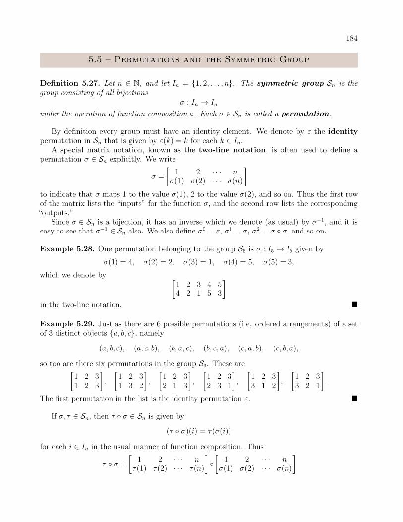
184

5.5 – Permutations and the Symmetric Group

Definition 5.27. Let n ∈ N, and let In = {1, 2, . . . , n}. The symmetric group Sn is thegroup consisting of all bijections

σ : In → In

under the operation of function composition ◦. Each σ ∈ Sn is called a permutation.

By definition every group must have an identity element. We denote by ε the identitypermutation in Sn that is given by ε(k) = k for each k ∈ In.

A special matrix notation, known as the two-line notation, is often used to define apermutation σ ∈ Sn explicitly. We write

σ =

[1 2 · · · n

σ(1) σ(2) · · · σ(n)

]to indicate that σ maps 1 to the value σ(1), 2 to the value σ(2), and so on. Thus the first rowof the matrix lists the “inputs” for the function σ, and the second row lists the corresponding“outputs.”

Since σ ∈ Sn is a bijection, it has an inverse which we denote (as usual) by σ−1, and it iseasy to see that σ−1 ∈ Sn also. We also define σ0 = ε, σ1 = σ, σ2 = σ ◦ σ, and so on.

Example 5.28. One permutation belonging to the group S5 is σ : I5 → I5 given by

σ(1) = 4, σ(2) = 2, σ(3) = 1, σ(4) = 5, σ(5) = 3,

which we denote by [1 2 3 4 54 2 1 5 3

]in the two-line notation. �

Example 5.29. Just as there are 6 possible permutations (i.e. ordered arrangements) of a setof 3 distinct objects {a, b, c}, namely

(a, b, c), (a, c, b), (b, a, c), (b, c, a), (c, a, b), (c, b, a),

so too are there six permutations in the group S3. These are[1 2 31 2 3

],

[1 2 31 3 2

],

[1 2 32 1 3

],

[1 2 32 3 1

],

[1 2 33 1 2

],

[1 2 33 2 1

].

The first permutation in the list is the identity permutation ε. �

If σ, τ ∈ Sn, then τ ◦ σ ∈ Sn is given by

(τ ◦ σ)(i) = τ(σ(i))

for each i ∈ In in the usual manner of function composition. Thus

τ ◦ σ =

[1 2 · · · n

τ(1) τ(2) · · · τ(n)

]◦[

1 2 · · · nσ(1) σ(2) · · · σ(n)

]

185

=

[1 2 · · · n

τ(σ(1)) τ(σ(2)) · · · τ(σ(n))

].

Example 5.30. In S3 we have[1 2 31 3 2

]◦[

1 2 33 2 1

]=

[1 2 32 3 1

], (5.21)

Note that the matrix immediately to the right of the symbol ◦ in (5.21) takes the input first, so

1→[

1 2 33 2 1

]→ 3→

[1 2 31 3 2

]→ 2,

which gives the first column of the matrix to the right of the = symbol in (5.21). �

Assuming n ≥ 2, a transposition is a permutation τ ∈ Sn for which there exist k, ` ∈ Inwith k 6= ` such that

τ(i) =

i, if i ∈ In \ {k, `}k, if i = `

`, if i = k.

Thus a transposition interchanges precisely two distinct elements of In while leaving all otherelements fixed. The classic example in S2 is[

1 22 1

],

and an example in S4 is [1 2 3 41 4 3 2

].

Any permutation σ ∈ Sn is uniquely determined by the arrangement of the elements of In inthe second row of its corresponding matrix. Since the n elements in In have n! possible distinctarrangements, it follows that Sn itself has n! elements. This proves the following.

Proposition 5.31. |Sn| = n! for all n ∈ N.

We now introduce another notation for elements of Sn called cycle notation. For m ≤ nlet J = {j1, j2, j3, . . . , jm} be a set of distinct elements of In. Then the symbol

(j1, j2, j3, . . . , jm), (5.22)

denotes a permutation in Sn that performs the mappings

j1 7→ j2 7→ j3 7→ · · · 7→ jm−1 7→ jm 7→ j1,

and also i 7→ i for any i ∈ In \ J . Using function notation, if σ ∈ Sn is such that

σ = (j1, j2, j3, . . . , jm),

thenσ(j1) = j2, σ(j2) = j3, . . . , σ(jm−1) = jm, σ(jm) = j1,

with σ(i) = i for any i ∈ In \ J .

186

Any permutation expressible in the form (5.22) is called a cycle. The entries in (5.22) areideally envisioned as being written in a circular arrangement, like the numbers on a clock, sothat the “last” entry jm is naturally seen to be followed by j1. In this way

(jm, j1, j2, . . . , jm−1)

is easily recognized as being the same permutation as that given by (5.22).

Example 5.32. In S3 the cycle (1, 3, 2) is the permutation[1 2 33 1 2

].

In S5 the cycle (1, 3, 2) is the permutation[1 2 3 4 53 1 2 4 5

].

Since (1, 3, 2) ∈ S5 does not feature 4 or 5 among its entries, we see that (1, 3, 2) maps 4 7→ 4and 5 7→ 5.

In Sn for any n ≥ 3 we have

(1, 3, 2) = (2, 1, 3) = (3, 2, 1).

That is, moving the last entry in a cycle to the first position does not change the correspondingpermutation. �

As with permutations in general, two cycles σ and τ in Sn may be composed. If

σ = (j1, j2, . . . , jm) and τ = (i1, i2, . . . , i`), (5.23)

then

(j1, j2, . . . , jm) ◦ (i1, i2, . . . , i`)

is the permutation σ ◦ τ . Typically the symbol ◦ is omitted in the cycle notation, and we write

σ ◦ τ = (j1, j2, . . . , jm)(i1, i2, . . . , i`).

The length of a cycle is simply the number of entries it contains. For instance the cycles σand τ in (5.23) have lengths m and `, respectively. We will say a cycle is an m-cycle if it haslength m. We now gather a few facts about transpositions.

Proposition 5.33. Let n ≥ 2.

1. S1 has no transpositions.2. τ ∈ Sn is a transposition if and only if τ is a 2-cycle.3. If τ ∈ Sn is a transposition, then τ ◦ τ = ε.4. If τ1, τ2 ∈ Sn are transpositions, then τ1 ◦ τ2 = τ2 ◦ τ1.

187

Proof.Proof of (3). Suppose τ ∈ Sn is a transposition, so τ = (a, b) for some a, b ∈ In with a 6= b bypart (2). Then

(τ ◦ τ)(a) = τ(τ(a)) = τ(b) = a and (τ ◦ τ)(b) = τ(τ(b)) = τ(a) = b,

and furthermore(τ ◦ τ)(i) = τ(τ(i)) = τ(i) = i

for any i ∈ In \ {a, b}. Therefore τ ◦ τ = ε. �

Proofs of the other parts of Proposition 5.33 are left as exercises.Two cycles (j1, . . . , jm) and (i1, . . . , i`) in Sn are disjoint if

{j1, . . . , jm} ∩ {i1, . . . , i`} = ∅,

which is to say the cycles have no entries in common. Thus (1, 6, 3) and (4, 2, 5, 8) are disjoint since{1, 6, 3}∩{4, 2, 5, 8} = ∅, but (5, 2, 1) and (3, 1, 9, 2) are not disjoint since {5, 2, 1}∩{3, 1, 9, 2} ={1, 2}.

Proposition 5.34. If (j1, . . . , jm) and (i1, . . . , i`) are disjoint cycles in Sn, then

(j1, . . . , jm)(i1, . . . , i`) = (i1, . . . , i`)(j1, . . . , jm).

The proof of Proposition 5.34 is left as an exercise. Another way to state Proposition 5.34 is tosay that disjoint cycles commute. Parts (2) and (4) of Proposition 5.33 imply that commutativityalways holds in the special case of 2-cycles, even if the 2-cycles under consideration are notdisjoint.

The process of expressing a permutation as a composition of two or more cycles is knownas cycle decomposition. Even a permutation that is itself a cycle we may be interested inexpressing anew as a composition of two cycles of lesser length. Indeed, of particular importanceto us along our path to a new formulation for determinants in the next section is the process ofdecomposing a permutation into 2-cycles (i.e. transpositions).

Example 5.35. Consider the permutation

σ =

[1 2 3 4 5 6 73 6 1 2 5 7 4

]in S7. We see that σ maps 1 to 3, and also 3 back to 1. We may write this as 1 7→ 3 7→ 1. Wealso have the chain of mappings

2 7→ 6 7→ 7 7→ 4 7→ 2.

The only mapping left is 5 7→ 5. Thus σ has the cycle decomposition

(1, 3)(2, 6, 7, 4),

or equivalently (2, 6, 7, 4)(1, 3). Recall that if a value is absent from a cycle’s list of entries, thenthe cycle returns that value unchanged. Thus

5→ (1, 3)→ 5→ (2, 6, 7, 4)→ 5,

188

whereas

1→ (1, 3)→ 3→ (2, 6, 7, 4)→ 3.

To decompose σ into transpositions it is only necessary to decompose (2, 6, 7, 4) into trans-positions. In fact we have

(2, 6, 7, 4) = (2, 6)(2, 7)(2, 4),

where the three transpositions on the right-hand side may be written in any order, and so

σ = (1, 3)(2, 6, 7, 4) = (1, 3)(2, 6)(2, 7)(2, 4),

where again any order is permissible. �

It was not mere luck that the permutation σ in Example 5.35 was able to be decomposedinto transpositions. As the next proposition makes clear, this is true of any permutation in Snfor n ≥ 2.

Proposition 5.36. Let n ≥ 2. If σ ∈ Sn, then for some k ∈ N there exist transpositionsτ1, . . . , τk ∈ Sn such that

σ = τ1 ◦ · · · ◦ τk.

Proof. The proof will employ induction, so we start by showing the n = 2 case is true. Thesymmetric group S2 has only two elements: ε and (1, 2). Since (1, 2) is already a transposition,we need only show that

ε =

[1 21 2

]can be expressed as a composition of transpositions. But by Proposition 5.33(3) we immediatelyhave ε = (1, 2)(1, 2), and so we’re done.

Now let n ≥ 2 be arbitrary, and suppose the statement of the proposition holds for this valuen. Let σ ∈ Sn+1, so that

σ =

[1 2 · · · n+ 1i1 i2 · · · in+1

].

Since σ : In+1 → In+1 is a bijection there exists some m ∈ In+1 such that σ(m) = n+ 1. Thereare two cases to consider: either m = n+ 1 or m < n+ 1.

If m = n + 1, so that σ(n + 1) = n + 1, then σ(i) ∈ In for each i ∈ In. If we defineσ : In → In by σ(i) = σ(i) for each i ∈ In, then σ ∈ Sn, and by our inductive hypothesis thereexist transpositions τ1, . . . , τk ∈ Sn such that σ = τ1 ◦ · · · ◦ τk. By Proposition 5.33(2) eachtransposition τj is a 2-cycle (aj, bj), and since aj, bj ∈ In and In ⊆ In+1, it follows that (aj, bj)also defines a 2-cycle in Sn+1. Taking τj = (aj, bj) to be in Sn+1 for each 1 ≤ j ≤ k, we findthat σ = τ1 ◦ · · · ◦ τk, and so σ is expressible as a composition of transpositions.

Suppose next that m < n + 1, so σ(m) = n + 1 for m ∈ In. Defining σ0 ∈ Sn+1 byσ0 = σ ◦ (m,n+ 1), Proposition 5.33(3) and the known associativity of the function compositionoperation imply that

σ = σ ◦ ε = σ ◦ ((m,n+ 1) ◦ (m,n+ 1))

= (σ ◦ (m,n+ 1)) ◦ (m,n+ 1) = σ0 ◦ (m,n+ 1). (5.24)

189

Now, sinceσ0(n+ 1) = (σ ◦ (m,n+ 1))(n+ 1) = σ(m) = n+ 1,

we see that σ0 has the property treated in the m = n+ 1 case, and so by the same argumentused in that case there exist transpositions τ1, . . . , τk ∈ Sn+1 such that σ0 = τ1 ◦ · · · ◦ τk. Thenby (5.24) we find that

σ = τ1 ◦ · · · ◦ τk ◦ (m,n+ 1),

which shows that σ is again expressible as a composition of transpositions. �

What Proposition 5.36 does not say is that the cycle decomposition of a permutation intotranspositions is necessarily unique, and that’s because it never is. Even for (1, 2) ∈ S2 we have

(1, 2) = (1, 2)(1, 2)(1, 2) = (1, 2)(1, 2)(1, 2)(1, 2)(1, 2),

and in general (1, 2) = (1, 2)2k−1 for any k ∈ N.Is there anything more that can be said about the decomposition of a permutation into

transpositions, beyond its mere existence? Recall that any integer has a parity, which is tosay the integer is either even (divisible by 2) or odd (not divisible by 2). Now we define theparity of a particular decomposition of σ ∈ Sn into transpositions τ1, . . . , τk as being odd if kis odd, and even if k is even. The next proposition states that no one permutation can havetwo decompositions of opposite parity.

Proposition 5.37. Let n ≥ 2. If σ ∈ Sn, then the decompositions of σ into transpositions areeither all odd or all even.

Proof. The proof will employ induction, so we start by showing the n = 2 case is true. Thesymmetric group S2 has only two elements, ε and (1, 2), with (1, 2) in particular being the onlytransposition available. Now, for any k ≥ 0 Proposition 5.33(3) implies that

(1, 2)2k = [(1, 2)(1, 2)]k = εk = ε,

and(1, 2)2k+1 = (1, 2)(1, 2)2k = (1, 2) ◦ ε = (1, 2).

Thus all the possible even decompositions equal ε, and all the possible odd decompositions equal(1, 2). It follows that ε has only even decompositions, and (1, 2) has only odd decompositions.

Now let n ≥ 2 be arbitrary, and suppose the statement of the proposition holds for this valuen. The remainder of the proof we leave as an exercise. �

It is because of Proposition 5.37 that the following definition is meaningful.

Definition 5.38. Let n ≥ 2. A permutation σ ∈ Sn is even if it can be expressed as acomposition of an even number of transpositions, and odd if it can be expressed as a compositionof an odd number of transpositions. By definition ε ∈ S1 we take to be even.

The sign function on Sn is the function sgn : Sn → {−1, 1} given by

sgn(σ) =

{1, if σ is even

−1, if σ is odd.

190

The only element of S1 is

ε =

[11

],

which cannot be expressed as a composition of transpositions since there are no transpositionsin S1. Nonetheless it will be convenient to define ε ∈ S1 to be even, and therefore sgn(ε) = 1.

Remark. Since (−1)m is 1 if m is even and −1 if m is odd, we see from Definition 5.38 that ifa permutation σ can be expressed as a composition of m transpositions, then sgn(σ) = (−1)m.

It is straightforward to check that the composition of two even permutations is again even,and so if An is the set of all even permutations in Sn, then An is in fact a subgroup of Sn calledthe antisymmetric group. In contrast the composition of two odd permutations is even, andso the set Sn \ An of all odd permutations in Sn is not a group since it is not closed under theoperation ◦ of function composition.

191

5.6 – The Leibniz Formula

In §5.2 we found that, for each n ∈ N, the functions detn,i and det′n,j were equal for all1 ≤ i, j ≤ n; that is,

detn,1 = · · · = detn,n = det′n,1 = · · · = det′n,n .

That all these functions are the same ultimately derives from the fact that they all possess thesix properties given in Theorem 5.4. A close look at these properties, however, reveals that notall of them are fundamental. That is, some of the properties are an immediate consequence ofone or more of the others. In particular, analyzing the details of the theorem’s proof, it can beseen that properties DP1, DP2, and DP3 are independent (i.e. no two can be used to derive thethird), and yet taken together they readily imply DP4, DP5, and DP6.

While all the “different” determinants defined in §5.2 turned out to be the same, it isreasonable to wonder whether there is some way to define the determinant of a square matrix Aso that it possesses the properties in Theorem 5.4 and yet is genuinely different. Put anotherway, if the minimum qualifications that a function must satisfy in order for it to be called a“determinant” are that it possess the multilinearity, alternating, and normalization properties inTheorem 5.4, does that uniquely characterize the function? The answer is yes.

Theorem 5.39 (Uniqueness of the Determinant). For n ∈ N suppose D : Fn×n → F hasthe following properties:

DP1. Multilinearity. For any 1 ≤ j ≤ n and x ∈ F,

D(. . . , aj, . . .) +D(. . . ,bj, . . .) = D(. . . , aj + bj, . . .),

and

D(. . . , xaj, . . .) = xD(. . . , aj, . . .).

DP2. Alternating. For any 1 ≤ j < k ≤ n,

D(. . . , aj, . . . , ak, . . .) = −D(. . . , akj

, . . . , ajk

, . . .).

DP3. Normalization.

D(In) = 1.

Then D = detn.

Proof. Applying DP2 in the case when aj = ak = u gives

D(. . . ,u, . . . ,u, . . .) = −D(. . . ,u, . . . ,u, . . .),

and hence

D(. . . ,u, . . . ,u, . . .) = 0.

That is, D(A) = 0 whenever A ∈ Fn×n has two identical columns.Let A = [a1 · · · an] ∈ Fn×n be arbitrary. By DP1,

D(A) = D(a1, . . . , an) = D

(n∑

i1=1

ai11ei1 , . . . ,n∑

in=1

ainnein

)

192

=n∑

i1=1

· · ·n∑

in=1

D(ai11ei1 , . . . , ainnein

)=

n∑i1=1

· · ·n∑

in=1

ai11 · · · ainnD(ei1 , . . . , ein). (5.25)

It remains to evaluate D(ei1 , . . . , ein) in (5.25). In fact we have D(ei1 , . . . , ein) = 0 wheneverik = i` for some k 6= `, since the matrix [ei1 · · · ein ] then has two identical columns, and itfollows that only those terms in the sum (5.25) for which the list of values i1, . . . , in represents apermutation σ ∈ Sn are all that’s left. In particular, for each such term we take σ to be given byσ(k) = ik for 1 ≤ k ≤ n, and since there is a one-to-one correspondence between the remainingterms in (5.25) and the elements of Sn, we obtain

D(A) =∑σ∈Sn

aσ(1),1 · · · aσ(n),nD(eσ(1), . . . , eσ(n)). (5.26)

Now, for any σ ∈ Sn there exist, by Proposition 5.36, transpositions τ1, . . . , τm such thatσ = τm ◦ · · · ◦ τ1. By DP2,

D(e1, . . . , en) = −D(eτ1(1), . . . , eτ1(n)) = (−1)2D(eτ2(τ1(1)), . . . , eτ2(τ1(n)))

= (−1)3D(eτ3(τ2(τ1(1))), . . . , eτ3(τ2(τ1(n))))

...

= (−1)mD(e(τm◦···◦τ1)(1), . . . , e(τm◦···◦τ1)(n))

= sgn(σ)D(eσ(1), . . . , eσ(n)),

and so by DP3, noting that 1/ sgn(σ) = sgn(σ),

D(eσ(1), . . . , eσ(n)) = sgn(σ)D(e1, . . . , en) = sgn(σ)D(In) = sgn(σ).

Putting this result into (5.26) gives

D(A) =∑σ∈Sn

aσ(1),1 · · · aσ(n),n sgn(σ). (5.27)

The expression at right in (5.27) is entirely independent of D. Indeed, if we assume D isanother function on Fn×n that satisfies the properties DP1, DP2, and DP3, then an identicalargument will lead to D(A) equalling the same expression, and hence D(A) = D(A). Sincedetn has the properties DP1, DP2, and DP3, we conclude that detn(A) = D(A). �

The proof of Theorem 5.39 immediately gives the following result, which is a formula for thedeterminant function that is explicit rather than recursive.

Theorem 5.40 (Leibniz Formula). For any n ∈ N and A ∈ Fn×n,

detn(A) =∑σ∈Sn

sgn(σ)aσ(1),1aσ(2),2 · · · aσ(n),n.

193

Proposition 5.41. Let n ≥ 2. For any 1 ≤ k < ` ≤ n,∑σ∈Sn

sgn(σ)

(aσ(k),kaσ(`),k

∏i∈In\{k,`}

aσ(i),i

)= 0. (5.28)

Proof. Fix 1 ≤ k < ` ≤ n, and let Σσ denote the sum in (5.28). Then

Σσ =∑π∈An

(aπ(k),kaπ(`),k

∏i∈In\{k,`}

aπ(i),i

)−

∑ν∈Sn\An

(aν(k),kaν(`),k

∏i∈In\{k,`}

aν(i),i

). (5.29)

Fix π0 ∈ An. Then ν0 = π0 ◦ (k, `) ∈ Sn \ An is given by

ν0(i) =

π0(i), if i ∈ In \ {k, n}π0(`), if i = k

π0(k), if i = `,

so thataν0(`),kaν0(k),k

∏i∈In\{k,`}

aν0(i),i = aπ0(k),kaπ0(`),k∏

i∈In\{k,`}

aπ0(i),i.

This shows that the term in the sum∑

π∈An that corresponds to π0 is canceled by the term in∑ν∈Sn\An that corresponds to ν0 at right in (5.29). In a similar way, for any ν1 ∈ Sn \ An we

have π1 = ν1 ◦ (k, `) ∈ An, and the terms in∑

π∈An and∑

ν∈Sn\An corresponding to π1 and ν1will cancel in (5.29). Therefore the sum

∑σ must equal zero. �

194

6Eigen Theory

6.1 – Eigenvectors and Eigenvalues

Throughout this chapter we assume that all vector spaces are finite-dimensional withdimension at least 1 unless otherwise specified.

Definition 6.1. Let V be a vector space over F and L : V → V a linear operator. Aneigenvector of L is a nonzero vector v ∈ V such that

L(v) = λv

for some λ ∈ F. The scalar λ is an eigenvalue of L, and v is said to be an eigenvectorcorresponding to λ. The set

EL(λ) = {v ∈ V : L(v) = λv}

is the eigenspace of L corresponding to λ.

The symbol σ(L) will occasionally be used to denote the set of eigenvalues possessed by alinear operator L, so that |σ(L)| denotes the number of distinct eigenvalues of L.

A careful examination of Definition 6.1 should make it clear that, while the zero vector0 ∈ V cannot be an eigenvector, the zero scalar 0 ∈ F can be an eigenvalue. Despite not beingan eigenvector, however, it is always true that 0 is an element of EL(λ) since

L(0) = 0 = λ0

holds for any linear operator L

Proposition 6.2. Let V be a vector space. If L : V → V is a linear operator with eigenvalueλ, then EL(λ) is a subspace of V .

Proof. Suppose L : V → V is linear with eigenvalue λ. It has already been established that0 ∈ EL(λ). Given u,v ∈ EL(λ) and scalar c we have

L(u + v) = L(u) + L(v) = λu + λv = λ(u + v)

195

and

L(cv) = cL(v) = c(λv) = λ(cv),

which shows that u + v ∈ EL(λ) and cv ∈ EL(λ). �

Example 6.3. Let V be a vector space and consider the identity operator IV : V → V givenby IV (v) = v for all v ∈ V . It is clear that λ = 1 is the only eigenvalue of IV , and all nonzerovectors in V are corresponding eigenvectors. Indeed,

EIV (1) = {v ∈ V : IV (v) = v} = V

is the corresponding eigenspace. �

Example 6.4. Let V be a vector space and consider the zero operator OV : V → V given byOV (v) = 0 for all v ∈ V . For any v 6= 0, then, we have

OV (v) = 0 = 0v,

which shows that 0 is an eigenvalue of OV . Moreover

EOV (0) = {v ∈ V : OV (v) = 0v} = V

is the corresponding eigenspace. There are no other eigenvalues. �

In addition to eigenvectors, eigenvalues, and eigenspaces of linear mappings, there are relatednotions for square matrices.

Definition 6.5. Let A ∈ Fn×n. An eigenvector of A is a nonzero vector x ∈ Fn such that

Ax = λx

for some λ ∈ F. The scalar λ is an eigenvalue of A, and x is said to be an eigenvectorcorresponding to λ. The set

EA(λ) = {x ∈ Fn : Ax = λx}is the eigenspace of A corresponding to λ.

The symbol σ(A) will occasionally be used to denote the set of eigenvalues possessed by asquare matrix A, so that |σ(A)| denotes the number of distinct eigenvalues of A.

Remark. A careful reading of Definition 6.5 should make it clear that any eigenvector corre-sponding to an eigenvalue of A ∈ Fn×n must be an element of Fn. Thus, if we are given thatA ∈ Rn×n, then we would discount any z ∈ Cn \ Rn for which Az = λz for some λ ∈ R.

Proposition 6.6. If λ is an eigenvalue of A ∈ Fn×n, then EA(λ) is a subspace of Fn.

196

Proof. Suppose that λ is an eigenvalue of A. By Definitions 6.5 and 3.15,

x ∈ EA(λ) ⇔ Ax = λx ⇔ Ax− λx = 0 ⇔ Ax− λInx = 0

⇔ (A− λIn)x = 0 ⇔ x ∈ Nul(A− λIn).

That is,EA(λ) = Nul(A− λIn), (6.1)

the null space of A− λIn. By Proposition 3.16 Nul(A− λIn) is a subspace of Fn, and hence sotoo is EA(λ). �

Proposition 6.7. Let V be a vector space over F, and suppose L ∈ L(V ) has eigenvalues λ1, λ2with corresponding eigenvectors v1,v2, respectively.

1. If λ1 6= λ2, then v1 6= v2.2. EL(λ1) ∩ EL(λ2) = {0} if and only if λ1 6= λ2.

Proof.Proof of Part (1). We will prove the contrapositive: “If v1 = v2, then λ1 = λ2.” Suppose thatv1 = v2 = v, so

λ1v = λ1v1 = L(v1) = L(v2) = λ2v2 = λ2v,

and then(λ1 − λ2)v = λ1v − λ2v = 0.

By Proposition 3.2(3) either λ1 − λ2 = 0 or v = 0. But v 6= 0 since an eigenvector is nonzeroby definition, and so it must be that λ1 − λ2. Therefore λ1 = λ2.

Proof of Part (2). Suppose λ1 = λ2 = λ, so that λ is an eigenvalue of L with correspondingeigenvectors v1 and v2. In particular

v1 ∈ EL(λ) = EL(λ1) = EL(λ2),

and thusv1 ∈ EL(λ1) ∩ EL(λ2).

Since v1 6= 0, it follows that EL(λ1) ∩ EL(λ2) 6= {0}.For the converse, suppose λ1 6= λ2. Let v ∈ EL(λ1) ∩ EL(λ2). Then L(v) = λ1v and

L(v) = λ2v, and thus λ1v = λ2v. Now,

λ1v = λ2v ⇒ (λ1 − λ2)v = 0,

and since λ1 − λ2 6= 0, Proposition 3.2(3) implies that v = 0. Therefore EL(λ1) ∩ EL(λ2) ={0}. �

The converse of Proposition 6.7(1) is not true in general; that is, if L ∈ L(V ) has eigenvaluesλ1, λ2 with corresponding eigenvectors v1,v2, then v1 6= v2 does not necessarily imply thatλ1 6= λ2. Consider for example v2 = 2v1: certainly v1 6= v2 since we know v1 6= 0, but

L(v2) = L(2v1) = 2L(v1) = 2(λ1v1) = λ1(2v1) = λ1v2

shows that λ1 = λ2.

197

Theorem 6.8. Let V be a vector space over F, and let L ∈ L(V ) have distinct eigenvaluesλ1, . . . , λn ∈ F. If v1, . . . ,vn are eigenvectors corresponding to λ1, . . . , λn, respectively, then theset {v1, . . . ,vn} is linearly independent.

Proof. An eigenvector is nonzero by definition, so if n = 1 then certainly the set {v1} is linearlyindependent. This establishes the base case of an inductive argument.

Suppose the theorem is true when n = m, where m is some arbitrary positive integer (thisis our “inductive hypothesis”). Let L be a linear operator on V with distinct eigenvaluesλ1, . . . , λm+1 and corresponding eigenvectors v1, . . . ,vm+1, so that L(vk) = λkvk for each1 ≤ k ≤ m+ 1. Suppose c1, . . . , cm+1 ∈ F are such that

m+1∑k=1

ckvk = 0. (6.2)

Since the eigenvalues λ1, . . . , λm+1 are distinct, there exists some 1 ≤ k0 ≤ m + 1 such thatλk0 6= 0. Since the eigenvalues may be indexed in any convenient way, we can assume k0 = m+ 1so that λm+1 6= 0. Multiplying (6.2) by λm+1 gives

m+1∑k=1

ckλm+1vk = 0, (6.3)

and we also have

L

(m+1∑k=1

ckvk

)= L(0) ⇒

m+1∑k=1

ckL(vk) = 0 ⇒m+1∑k=1

ckλkvk = 0. (6.4)

Subtracting (6.3) from the rightmost equation in (6.4), we obtain

m+1∑k=1

ckλkvk −m+1∑k=1

ckλm+1vk = 0,

so thatm+1∑k=1

ck(λk − λm+1)vk = 0. (6.5)

Of course

ck(λk − λm+1)vk = 0

if k = m+ 1, and so (6.5) becomes

m∑k=1

ck(λk − λm+1)vk = 0. (6.6)

Now, v1, . . . ,vm are the eigenvectors corresponding to the distinct eigenvalues λ1, . . . , λm, andso by our inductive hypothesis the set {v1, . . . ,vm} is linearly independent. From (6.6) it followsthat

ck(λk − λm+1) = 0

198

for 1 ≤ k ≤ m, which in turn implies that ck = 0 for 1 ≤ k ≤ m since λ1, . . . , λm do not equalλm+1. Now (6.2) becomes cm+1vm+1 = 0, which immediately yields cm+1 = 0. Since (6.2) resultsonly in the trivial solution

c1 = · · · = cm+1 = 0

we conclude that v1, . . . ,vm+1 are linearly independent.We see now that the theorem holds for n = m+ 1 when we assume that it holds for n = m,

and therefore by induction it holds for all n ∈ N. �

Corollary 6.9. If V is a finite-dimensional vector space and L ∈ L(V ), then L has at mostdim(V ) distinct eigenvalues.

Proof. Suppose that V is an n-dimensional vector space and L ∈ L(V ). Suppose λ1, . . . , λn+1

are distinct eigenvalues of L with corresponding eigenvectors v1, . . . ,vn+1. Then {v1, . . . ,vn+1}is a basis for V by Theorem 6.8 and we are led to conclude that the dimension of V is n+ 1,which is a contradiction. Therefore L has at most n distinct eigenvalues. �

Example 6.10. Let A ∈ Fn×n be the diagonal matrix

A =

λ1 · · · 0...

. . ....

0 · · · λn

having distinct diagonal entries λ1, . . . , λn (i.e. λi 6= λj whenever i 6= j). If e1, . . . , en are thestandard basis vectors for Fn, so that

e1 =

10...0

, e2 =

01...0

, . . . , en =

00...1

,then for each 1 ≤ k ≤ n we find that Aek = λkek, and so λk is an eigenvalue of A.

If L is the linear operator on Fn having A as its corresponding matrix with respect tothe standard basis E = {e1, . . . , en}, then clearly λ1, . . . , λn are distinct eigenvalues of L, withe1, . . . , en being corresponding eigenvectors:

L(ek) = Aek = λkek.

Of course the eigenvectors e1, . . . , en are linearly independent as predicted by Theorem 6.8. �

Proposition 6.11. An operator L ∈ L(V ) is not invertible if and only if 0 is an eigenvalue ofL. A matrix A ∈ Fn×n is not invertible if and only if 0 is an eigenvalue of A.

Proof. By the Invertible Operator Theorem (Theorem 4.65), L is not invertible if and only ifNul(L) 6= {0}, and Nul(L) 6= {0} if and only if there exists some v 6= 0 such that L(v) = 0,which is to say 0 is an eigenvalue of L since 0 = 0v.

By the Invertible Matrix Theorem (Theorem 5.17), A is not invertible if and only ifNul(A) 6= {0}, and Nul(A) 6= {0} if and only if there exists some x 6= 0 such that Ax = 0,which is to say 0 is an eigenvalue of A since 0 = 0x. �

199

Proposition 6.12. Let L ∈ L(V ) and A ∈ Fn×n.

1. Let n ∈ N. If λ is an eigenvalue of L (resp. A) with corresponding eigenvector v, then λn isan eigenvalue of Ln (resp. An) with eigenvector v.

2. Suppose L and A are invertible. If λ is an eigenvalue of L (resp. A) with correspondingeigenvector v, then λ−1 is an eigenvalue of L−1 (resp. A−1) with eigenvector v.

The proof will consider only the statements about an operator L : V → V , since thearguments are much the same for a square matrix A.

Proof.Proof of Part (1): The n = 1 case is trivially true. Suppose the statement of Part (1) is true forsome arbitrary n ∈ N. Let λ be an eigenvalue of L with corresponding eigenvector v. ThenL(v) = λv, and by our inductive hypothesis Ln(v) = λnv. Now,

Ln+1(v) = Ln(L(v)) = Ln(λv) = λLn(v) = λ(λnv) = λn+1v,

and Part (1) is proven for all n ∈ N by the principle of induction.

Proof of Part (2): Suppose that λ is an eigenvalue of L with corresponding eigenvector v, sothat L(v) = λv. By Proposition 4.55 we obtain L−1(λv) = v, and since λ 6= 0 by Proposition6.11, it follows that

L−1(λv) = v ⇒ λL−1(v) = v ⇒ L−1(v) = λ−1v.

Hence λ−1 is an eigenvalue of L−1. �

200

6.2 – The Characteristic Polynomial

Definition 6.13. Let A ∈ Fn×n. The characteristic polynomial of A is the polynomialfunction PA : F→ F given by

PA(t) = detn(A− tIn).

Some books define the characteristic polynomial of A to be det(tIn − A) instead ofdet(A − tIn), but whichever way it is done will have no impact on either the theory ofcharacteristic polynomials or any application involving them. This is because only the zeros ofthe characteristic polynomial will be of any concern. Setting QA(t) = det(tIn −A), observethat PA = QA if n is even, and PA = −QA if n is odd. In either case PA and QA will have thesame zeros.

Proposition 6.14. Let V be a vector space over F with dim(V ) = n, and let L ∈ L(V ). Thenthe following statements are equivalent.

1. λ is an eigenvalue of L with corresponding eigenvector u.2. There exists some basis B for V such that λ is an eigenvalue of [L]B with corresponding

eigenvector [u]B.3. For all bases B for V , λ is an eigenvalue of [L]B with corresponding eigenvector [u]B.

Proof.(1)⇒ (3): Suppose that λ is an eigenvalue of L, so there exists some u 6= 0 such that L(u) = λu.Let B be any basis for V , and let [L]B ∈ Fn×n be the matrix corresponding to L with respect toB, so that

[L]B[v]B = [L(v)]B

for all v ∈ V . Recall that by Theorem 4.11 the coordinate map V → Fn given by v 7→ [v]B isan isomorphism, so [u]B ∈ Fn is not the zero vector since Nul([ · ]B) = {0}. Thus, from

[L]B[u]B = [L(u)]B = [λu]B = λ[u]B

we conclude that λ is an eigenvalue of [L]B with corresponding eigenvector [u]B.

(3) ⇒ (2): This is obvious.

(2) ⇒ (1): Suppose there exists some basis B for V such that λ is an eigenvalue of [L]B withcorresponding eigenvector [u]B. Again, the coordinate map [ · ]B : V → Fn is an isomorphism, so

[L]B[u]B = λ[u]B ⇒ [L(u)]B = [λu]B ⇒ L(u) = λu,

where the last implication follows from the fact that [ · ]B : V → Fn is injective. Therefore λ isan eigenvalue of L with corresponding eigenvector u. �

We see from the proposition that if we consider two different bases B and B′ for V , thenthe matrices corresponding to L with respect to these bases, [L]B and [L]B′ , have the sameeigenvalues as L. The only thing that changes is the corresponding eigenvector: [v]B is an

201

eigenvector of [L]B corresponding to eigenvalue λ if and only if [v]B′ is an eigenvector of [L]B′corresponding to eigenvalue λ.

But there’s something more: the characteristic polynomials of [L]B and [L]B′ will be foundto be the same! To see this, recall IBB′ , the change of basis matrix from B to B′. By Corollary4.33 we have

[L]B′ = IBB′ [L]BI−1BB′ .

Now, noting that In = IBB′InI−1BB′ and

det(IBB′) det(I−1BB′) = det(IBB′) ·1

det(IBB′)= 1

by Theorem 5.24, for any t ∈ F we have

P[L]B′(t) = det([L]B′ − tIn) = det

(IBB′ [L]BI

−1BB′ − t(IBB′InI

−1BB′)

)= det

((IBB′ [L]B − t(IBB′In))I−1BB′

)= det

((IBB′ [L]B − IBB′(tIn))I−1BB′

)= det

(IBB′([L]B − tIn)I−1BB′

)= det(IBB′) det([L]B − tIn) det(I−1BB′)

= det([L]B − tIn) = P[L]B(t)

by Theorem 5.23. That is, P[L]B′= P[L]B , which is to say that the characteristic polynomial of

a linear operator’s associated matrix is invariant under change of basis. We have proven thefollowing.

Proposition 6.15. Let L : V → V be a linear operator, and let B and B′ be bases for V . If[L]B and [L]B′ are the matrices corresponding to L with respect to B and B′, then P [L]B = P [L]B′

.

Because of Proposition 6.15, it makes sense to speak of the “characteristic polynomial” of alinear operator on V without reference to any specific basis for V .

Definition 6.16. Let L be a linear operator on V . The characteristic polynomial of L isthe polynomial function PL : F→ F given by

PL(t) = P [L](t),

where [L] is the matrix corresponding to L with respect to any basis for V .

While the idea of an eigenvalue is simple, it can be quite difficult to find eigenvalues of eithera linear operator or a matrix by direct means. To help find the eigenvalue of a linear operatorwe have the following.

Theorem 6.17. Let L : V → V be a linear operator. Then λ is an eigenvalue of L if and onlyif L− λIV is not invertible.

Proof. Suppose that λ is an eigenvalue of L. Then there exists some v ∈ V such that v 6= 0and L(v) = λv. Now,

(L− λIV )(v) = L(v)− (λIV )(v) = λv − λIV (v) = λv − λv = 0,

202

which shows that v ∈ Nul(L−λIV ) and so Nul(L−λIV ) 6= {0}. Hence L−λIV is not invertibleby the Invertible Operator Theorem.

For the converse, suppose that L − λIV is not invertible. Then Nul(L − λIV ) 6= {0}by the Invertible Operator Theorem, and it follows that there exists some v 6= 0 such that(L− λIV )(v) = 0. Now,

(L− λIV )(v) = 0 ⇔ L(v)− λIV (v) = 0 ⇔ L(v)− λv = 0 ⇔ L(v) = λv,

and therefore λ is an eigenvalue of L. �

The next theorem plainly reduces the problem of finding eigenvalues of an n× n matrix tothat of finding the zeros of an nth-degree polynomial function. We begin to see the utility ofcharacteristic polynomials at this point.

Theorem 6.18. Let A ∈ Fn×n. Then λ is an eigenvalue of A if and only if PA(λ) = 0.

Proof. Suppose that λ is an eigenvalue of A, so that Ax0 = λx0 for some x0 ∈ Fn. Define thelinear mapping L : Fn → Fn by L(x) = Ax. Then

L(x0) = Ax0 = λx0

shows that λ is an eigenvalue of L, and so by Theorem 6.17 the mapping

L− λIFn : Fn → Fn

is not invertible. Let I = IFn , and observe that the matrix associated with L− λI is A− λIn:

(L− λI)(x) = L(x)− λI(x) = Ax− λx = Ax− λInx = (A− λIn)x

for all x ∈ Fn. Thus, since the operator L− λI is not invertible, by Corollary 4.59 its associatedsquare matrix A− λIn is also not invertible, and so det(A− λIn) = 0 by the Invertible MatrixTheorem. That is, PA(λ) = 0.

Conversely, suppose that PA(λ) = 0. Then det(A− λIn) = 0, so by the Invertible MatrixTheorem A− λIn is not invertible. Define L : Fn → Fn by L(x) = Ax. Then A− λIn is thematrix corresponding to the linear operator L− λI : Fn → Fn, and by Corollary 4.59 L− λIis not invertible. So λ is an eigenvalue of L by Theorem 6.17, which is to say there existssome nonzero x0 ∈ Fn such that L(x0) = λx0. Hence Ax0 = λx0 and we conclude that λ is aneigenvalue of A. �

Example 6.19. Find the characteristic polynomial PA : R→ R of

A =

1 −3 33 −5 36 −6 4

,find the eigenvalues of A, and find a basis for each eigenspace as a subspace of R3.

203

Solution. We have

PA(t) = det(A− tI3) = det

1 −3 33 −5 36 −6 4

− t 0 0

0 t 00 0 t

=

∣∣∣∣∣∣1− t −3 3

3 −5− t 36 −6 4− t

∣∣∣∣∣∣c1+c2→c2=======

∣∣∣∣∣∣1− t −2− t 3

3 −2− t 36 0 4− t

∣∣∣∣∣∣ −r1+r2→r2========

∣∣∣∣∣∣1− t −2− t 3t+ 2 0 0

6 0 4− t

∣∣∣∣∣∣ .Expanding the determinant according to the 2nd row then gives

PA(t) = (−1)2+1(t+ 2)

∣∣∣∣−2− t 30 4− t

∣∣∣∣ = (t+ 2)2(t− 4),

and so we see that PA(t) = 0 for t = −2, 4. Thus by Theorem 6.18 the eigenvalues of A areλ = −2, 4.

By (6.1) the eigenspace of A corresponding to λ = −2 is

EA(−2) = Nul(A + 2I3) = {x ∈ R3 : (A + 2I3)x = 0}

=

x1x2x3

∈ R3 :

3 −3 33 −3 36 −6 6

x1x2x3

=

000

.Writing the matrix equation—which is a homogeneous system of equations—as an augmentedmatrix, we have3 −3 3 0

3 −3 3 06 −6 6 0

−r1+r2→r2−−−−−−−−→−2r1+r3→r3

3 −3 3 00 0 0 00 0 0 0

13r1→r1−−−−−→

1 −1 1 00 0 0 00 0 0 0

. (6.7)

Hence x1 − x2 + x3 = 0, which implies that x3 = x2 − x1 and so

EA(−2) =

x1x2x3

∈ R3 : x1 − x2 + x3 = 0

=

x1

x2x2 − x1

: x1, x2 ∈ R

.Observing that x1

x2x2 − x1

=

x10−x1

+

0x2x2

=

10−1

x1 +

011

x2,we have

EA(−2) =

1

0−1

x1 +

011

x2 : x1, x2 ∈ R

and so it is clear that

B−2 =

1

0−1

,0

11

is a linearly independent set of vectors that spans EA(−2) and therefore must be a basis forEA(−2). Notice that the elements of B−2 are in fact eigenvectors of A corresponding to theeigenvalue −2, as are all the vectors belonging to EA(−2).

204

Next, the eigenspace of A corresponding to λ = 4 is

EA(4) = Nul(A− 4I3) = {x ∈ R3 : (A− 4I3)x = 0}

=

x1x2x3

∈ R3 :

−3 −3 33 −9 36 −6 0

x1x2x3

=

000

.Applying Gaussian Elimination to the corresponding augmented matrix yields−3 −3 3 0

3 −9 3 06 −6 0 0

r1+r2→r2−−−−−−−→2r1+r3→r3

−3 −3 3 00 −12 6 00 −12 6 0

−r2+r3→r3−−−−−−−−→− 1

2r2+r1→r1

−3 3 0 00 −12 6 00 0 0 0

.From the top row we obtain x2 = x1, and from the middle row we obtain x3 = 2x2 and thusx3 = 2x1. Now,

EA(4) =

x1x12x1

: x1 ∈ R

=

1

12

x1 : x1 ∈ R

.Clearly

B4 =

1

12

is a linearly independent set that spans EA(4) and so qualifies as a basis for EA(4). The vectorbelonging to B4 is an eigenvector of A corresponding to the eigenvalue 4, as is any real scalarmultiple of the vector. �

In Example 6.19 we found in (6.7) that A + 2I3 is row-equivalent to

B =

1 −1 10 0 00 0 0

,which clearly has rank 1, and so

rank(A + 2I3) = rank(B) = 1

by Theorem 3.66. Then by the Rank-Nullity Theorem for Matrices we have

dim(EA(−2)) = nullity(A + 2I3) = dim(R3)− rank(A + 2I3) = 3− 1 = 2. (6.8)

Then, employing the equation x1 − x2 + x3 = 0 obtained at right in (6.7), we could have easilyobtained the two solutions 1

10

and

011

.Since these two vectors in EA(−2) are linearly independent and we know from (6.8) that EA(−2)has dimension 2, we can conclude by Theorem 3.54(1) that the two vectors must be a basis forEA(−2). We mention this here in order to suggest an alternative means of finding a basis foran eigenspace which makes use of earlier theoretical developments.

205

In the next example, for variety’s sake, eigenspaces will be found using Definition 6.5 directly,rather than equation (6.1).

Example 6.20. Find the eigenvalues of the matrix

A =

−1 4 −2−3 4 0−3 1 3

,and also find a basis for each eigenspace as a subspace of R3.

Solution. Expanding the determinant according to the second row, we have

PA(t) = det(A− tI3) =

∣∣∣∣∣∣−1− t 4 −2−3 4− t 0−3 1 3− t

∣∣∣∣∣∣= (−1)2+1(−3)

∣∣∣∣4 −21 3− t

∣∣∣∣+ (−1)2+2(4− t)∣∣∣∣−1− t −2−3 3− t

∣∣∣∣= −t3 + 6t2 − 11t+ 6,

and so

PA(t) = 0 ⇔ t3 − 6t2 + 11t− 6 = 0.

By the Rational Zeros Theorem of algebra, the only rational numbers that may be zeros of PA

are ±1, ±2, ±3 and ±6. It’s an easy matter to verify that 1 is in fact a zero, and so by theFactor Theorem of algebra t− 1 must be a factor of PA(t). Now,

t3 − 6t2 + 11t− 6

t− 1= t2 − 5t+ 6,

whence we obtain

t3 − 6t2 + 11t− 6 = 0 ⇔ (t− 1)(t2 − 5t+ 6) = 0 ⇔ (t− 1)(t− 2)(t− 3) = 0,

and therefore PA(t) = 0 if and only if t = 1, 2, 3. By Theorem 6.18 the eigenvalues of A areλ = 1, 2, 3.

The eigenspace of A corresponding to λ = 1 is

EA(1) = {x ∈ R3 : Ax = x} =

xyz

∈ R3 :

−1 4 −2−3 4 0−3 1 3

xyz

=

xyz

.The matrix equation yields the system of equations −x+ 4y − 2z = x

−3x+ 4y = y−3x+ y + 3z = z

206

or equivalently −x+ 2y − 1z = 0−x+ y = 0−3x+ y + 2z = 0

Apply Gaussian elimination on the corresponding augmented matrix:−1 2 −1 0−1 1 0 0−3 1 2 0

−r1+r2→r2−−−−−−−−→−3r1+r3→r3

−1 2 −1 00 −1 1 00 −5 5 0

−5r2+r3→r3−−−−−−−−→

−1 2 −1 00 −1 1 00 0 0 0

,so from the second row we have y = z, and from the first row we have x = 2y − z = 2z − z = z.Replacing z with t, so that x = y = z = t, we have

EA(1) =

ttt

: t ∈ R

=

1

11

t : t ∈ R

.From this we see that the set

B1 =

1

11

is a basis for EA(1).

The eigenspace of A corresponding to λ = 2 is

EA(2) = {x ∈ R3 : Ax = 2x} =

xyz

∈ R3 :

−1 4 −2−3 4 0−3 1 3

xyz

=

2x2y2z

.The matrix equation yields the system of equations−3x+ 4y − 2z = 0

−3x+ 2y = 0−3x+ y + z = 0

Apply Gaussian elimination on the corresponding augmented matrix:−3 4 −2 0−3 2 0 0−3 1 1 0

−r1+r2→r2−−−−−−−→−r1+r3→r3

−3 4 −2 00 −2 2 00 −3 3 0

− 32r2+r3→r3−−−−−−−−→

−3 4 −2 00 −2 2 00 0 0 0

,so from the second row we have y = z, and from the first row we have

x =4

3y − 2

3z =

4

3z − 2

3z =

2

3z.

Hence

EA(2) =

2z/3

zz

: z ∈ R

=

2/3

11

z : z ∈ R

.

207

If we replace z with 3t, we obtain an equivalent rendition of E2 that features no fractions:

EA(2) =

2

33

t : t ∈ R

.

The set

B2 =

2

33

is a basis for E2.

Finally, the eigenspace of A corresponding to λ = 3 is

EA(3) = {x ∈ R3 : Ax = 3x} =

xyz

∈ R3 :

−1 4 −2−3 4 0−3 1 3

xyz

=

3x3y3z

.The matrix equation yields the system of equations−4x+ 4y − 2z = 0

−3x+ y = 0−3x+ y = 0

Once more we apply Gaussian elimination to the augmented matrix:−4 4 −2 0−3 1 0 0−3 1 0 0

−r2+r3→r3−−−−−−−→12r1→r1

−2 2 −1 0−3 1 0 0

0 0 0 0

,so y = 3x and −2x+ 2y − z = 0, where

− 2x+ 2y − z = 0 ⇒ z = −2x+ 2y ⇒ z = 4x.

Therefore, replacing x with t so that y = 3t and z = 4t, we have

EA(3) =

1

34

t : t ∈ R

.The set

B3 =

1

34

is a basis for EA(3). �

Example 6.21. Find the eigenvalues of the matrix

A =

[2 3−1 4

],

and also find a basis for each eigenspace as a subspace of C2.

208

Solution. We have


∣∣∣∣ 2− t 3−1 4− t

∣∣∣∣ = t2 − 6t+ 11,

and soPA(t) = 0 ⇔ t2 − 6t+ 11 = 0 ⇔ t = 3± i

√2.

That is, A has two complex-valued eigenvalues. Let λ = 3− i√

2. The eigenspace correspondingto λ is

EA(λ) = {z ∈ C2 : Az = λz} =

{[z1z2

]∈ C2 :

[2 3−1 4

][z1z2

]=

[λz1λz2

]}.

Now, [2 3−1 4

][z1z2

]=

[λz1λz2

]corresponds to the system of equations{

(2− λ)z1 + 3z2 = 0−z1 + (4− λ)z2 = 0

We apply Gaussian elimination to the augmented matrix,[2− λ 3 0−1 4− λ 0

]r1↔r2−−−−→

[−1 4− λ 0

2− λ 3 0

](2−λ)r1+r2→r2−−−−−−−−−−→

[−1 4− λ 0

0 0 0

],

observing that

(2− λ)(4− λ) + 3 = (λ2 − 6λ+ 8) + 3 =(3− i

√2)2 − 6

(3− i

√2)

+ 11 = 0.

Thusz1 =

(− 1− i

√2)z2,

and so we obtain

EA(λ) =

{[(− 1− i

√2)z2

z2

]: z2 ∈ C

}=

{[−1− i

√2

1

]z : z ∈ C

},

where for simplicity we replace z2 with z in the end. Hence the eigenvector[−1− i

√2

1

]corresponding to the eigenvalue 3− i

√2 constitutes a basis for the eigenspace EA(λ).

The analysis of the other eigenvalue 3 + i√

2 is quite similar (with eigenspace also ofdimension 1) and so is left as a problem. �

Example 6.22. We will show that, for all n ∈ N, if A ∈ F is given by

A =

0 0 0 · · · 0 −a01 0 0 · · · 0 −a10 1 0 · · · 0 −a2...

......

. . ....

...0 0 0 · · · 0 −an−20 0 0 · · · 1 −an−1

, (6.9)

209

then

PA(t) = (−1)n(a0 + a1t+ · · ·+ an−1tn−1 + tn). (6.10)

In the case when n = 1 we take A = [−a0], whereupon we obtain

PA(t) = det1(A− tI1) = det1([−a0 − t]) = −a0 − t = (−1)(a0 + t).

This establishes the base case of an inductive argument. Fix n ∈ N, and suppose any matrix ofthe form (6.9) has characteristic polynomial (6.10); that is, detn(A− tIn) is given by∣∣∣∣∣∣∣∣∣∣∣∣

−t 0 0 · · · 0 −a01 −t 0 · · · 0 −a10 1 −t · · · 0 −a2...

......

. . ....

...0 0 0 · · · −t −an−20 0 0 · · · 1 −an−1 − t

∣∣∣∣∣∣∣∣∣∣∣∣= (−1)n(a0 + a1t+ · · ·+ an−1t

n−1 + tn).

Now, define A ∈ F(n+1)×(n+1) by

A =

0 0 0 · · · 0 −a01 0 0 · · · 0 −a10 1 0 · · · 0 −a2...

......

. . ....

...0 0 0 · · · 0 −an−10 0 0 · · · 1 −an

,so

A− tIn+1 =

−t 0 0 · · · 0 −a01 −t 0 · · · 0 −a10 1 −t · · · 0 −a2...

......

. . ....

...0 0 0 · · · −t −an−10 0 0 · · · 1 −an − t

.

Letting B = A− tIn+1,

PA(t) = detn+1(B) =n+1∑j=1

(−1)1+ja1j detn(B1j)

= −t detn(B11) + (−1)n+2(−a0) detn(B1(n+1)),

where

B11 =

−t 0 0 · · · 0 −a11 −t 0 · · · 0 −a20 1 −t · · · 0 −a3...

......

. . ....

...0 0 0 · · · −t −an−10 0 0 · · · 1 −an − t

and B1(n+1) =

1 −t 0 · · · 0 00 1 −t · · · 0 00 0 1 · · · 0 0...

......

. . ....

...0 0 0 · · · 1 −t0 0 0 · · · 0 1

.

210

Clearly detn(B1(n+1)) = 1, and by the inductive hypothesis we have

detn(B11) = (−1)n(a1 + a2t+ · · ·+ antn−1 + tn),

so that

PA(t) = −t(−1)n(a1 + a2t+ · · ·+ antn−1 + tn)− (−1)na0

= (−1)n+1(a1t+ a2t2 + · · ·+ ant

n + tn+1) + (−1)n+1a0

= (−1)n+1(a0 + a1t+ · · ·+ antn + tn+1),

as desired. �

Problems

1. For each of the 2× 2 matrices below, do the following:(i) Find the characteristic equation.

(ii) Find all real eigenvalues.(iii) Find a basis for the eigenspace corresponding to each real eigenvalue.

(a)

[3 08 −1

](b)

[0 34 0

](c)

[−2 −7

1 2

](d)

[0 00 0

]2. For each of the 3× 3 matrices below, do the following:

(i) Find the characteristic equation.(ii) Find all real eigenvalues.(iii) Find a basis for the eigenspace corresponding to each real eigenvalue.

(a)

4 0 1−2 1 0−2 0 1

(b)

3 0 −515−1 0

1 1 −2

(c)

5 6 20 −1 −81 0 −2

3. For each of the 4× 4 matrices below, do the following:

(i) Find the characteristic equation.(ii) Find all real eigenvalues.(iii) Find a basis for the eigenspace corresponding to each real eigenvalue.

(a)

0 0 2 01 0 1 00 1 −2 00 0 0 1

(b)

10 −9 0 04 −2 0 00 0 −2 −70 0 1 2

211

6.3 – Applications of the Characteristic Polynomial

Recall that Pn(F) denotes the set of polynomials of degree n with coefficients in F. That is,for n ∈W,

Pn(F) =

{n∑k=0

akxk : a0, . . . , an ∈ F and an 6= 0

}.

We regard 0 to be the polynomial of degree −1 and define P−1(F) = {0}. If F is an infinite fieldsuch as R or C, it is common to treat a polynomial as a function f : F→ F given by

f(x) =n∑k=0

akxk

for all x ∈ F, in which case it is called a polynomial function. For n ≥ −1, a polynomial functionp is said to have degree n if f(x) ∈ Pn(F), in which case we write deg(p) = n. Thus, we mayjust as well regard Pn(F) as the set of all polynomial functions of degree n, so that it makes asmuch sense to write f ∈ Pn(F) as f(x) ∈ Pn(F). Finally, we define

P(F) =∞⋃n=0

Pn−1(F).

In what follows we will have need of the following theorem, which is proven in §5.1 of theComplex Analysis Notes.

Theorem 6.23 (Fundamental Theorem of Algebra). If

p(z) = anzn + an−1z

n−1 + · · ·+ a1z + a0

is a polynomial function of degree n ≥ 1 with coefficients a0, . . . , an ∈ C, then there exists somez0 ∈ C such that p(z0) = 0.

Theorem 6.24 (Division Algorithm for Polynomials). Let f ∈ Pn(F), and let g ∈ Pm(F)for some m ≥ 0. Then there exist unique polynomial functions q and r such that

f(x) = q(x)g(x) + r(x)

for all x ∈ F, where deg(r) ≤ m.

Theorem 6.25 (Factor Theorem). Let f ∈ Pn(F) for some n ≥ 1, and let c ∈ F. Thenf(c) = 0 if and only if x− c is a factor of f(x).

Lemma 6.26. Suppose P(t) = [pij(t)]n ∈ Fn×n is such that pij is a polynomial function for all1 ≤ i, j ≤ n. If

deg(pij) ≤

{0, i 6= j

1, i = j

then deg(detn(P(t))) ≤ n.

http://faculty.bucks.edu/erickson/complex_analysis/complex5.pdf

212

Proof. The statement of the lemma is clearly true in the case when n = 1. Suppose that it istrue for some arbitrary n ∈ N. Let P(t) = [pij(t)]n+1. Then, expanding along the first row, wehave

detn+1(P(t)) =n+1∑j=1

(−1)1+jp1j(t) detn(P1j(t)).

For each 1 ≤ j ≤ n + 1 we find that the n × n submatrix P1j is such that all non-diagonalentries are degree 0 polynomial functions (i.e. constants), and all diagonal entries are polynomialfunctions of either degree 0 or degree 1. Thus deg(detn(P1j)) ≤ n by our inductive hypothesis,and since p1j(t) is a constant for 2 ≤ j ≤ n+ 1, it follows that

deg((−1)1+jp1j(t) detn(P1j(t))

)≤ n

for 2 ≤ j ≤ n+ 1. In the case when j = 1 we have

(−1)1+jp1j(t) detn(P1j(t)) = p11(t) detn(P11(t)),

where p11(t) has degree at most 1, and detn(P11(t)) has degree at most n. Hence

deg(p11(t) detn(P11(t))

)≤ n+ 1,

and therefore deg(detn(P(t))) ≤ n+ 1 since detn+1(P(t)) is the sum of polynomials of degree atmost n+ 1. Thus the lemma holds true in the n+ 1 case, and so it must hold for all n ∈ N byinduction. �

Proposition 6.27. If A ∈ Fn×n, then deg(PA) = n and the lead coefficient of PA is (−1)n.

Proof. In the case when n = 1 we have A = [a], so that

PA(t) = det1([a]− [t]) = det1([a− t]) = a− t = −t+ a,

and we clearly that deg(PA) = 1 and the lead coefficient of PA is (−1)1.Suppose the proposition is true for some n ∈ N. Let A = [aij]n+1 ∈ F(n+1)×(n+1), and define

P(t) = A− tIn+1 so that P(t) = [pij(t)]n+1 with

deg(pij) =

{0, i 6= j

1, i = j

Now,

PA(t) = detn+1(P(t)) =n+1∑k=1

(−1)1+kp1k(t) detn(P1k(t)),

where for each k we have P1k(t) = [pk,ij(t)]n such that

deg(pk,ij) ≤

{0, i 6= j

1, i = j

and so deg(detn(P1k(t))) ≤ n by Lemma 6.26. Since p1k(t) is a constant for 2 ≤ k ≤ n+ 1, itfollows that

deg((−1)1+kp1k(t) detn(P1k(t))

)≤ n

213

for 2 ≤ k ≤ n+ 1. In the case when k = 1 we have

(−1)1+kp1k(t) detn(P1k(t)) = p11(t) detn(P11(t)),

where

detn(P11(t)) = detn(A11 − tIn) = PA11(t)

has degree n and lead coefficient (−1)n by our inductive hypothesis. That is,

detn(P11(t)) = (−1)ntn + bn−1tn−1 + · · ·+ b1t+ b0

for some bn−1, . . . , b0 ∈ F, and since p11(t) = a11 − t we obtain

p11(t) detn(P11(t)) = (−t+ a11)((−1)ntn + bn−1t

n−1 + · · ·+ b1t+ b0)

= (−1)n+1tn+1 + cntn + · · ·+ c1t+ c0

for some cn, . . . , c0 ∈ F. Hence Q(t) = p11(t) detn(P11(t)) has degree n+ 1 with lead coefficient(−1)n+1. Since PA(t) = detn+1(P(t)) is the sum of Q(t) with other polynomials of degree atmost n, it follows that PA likewise has degree n+ 1 with lead coefficient (−1)n+1.

We conclude by the principle of induction that the proposition holds for all n ∈ N, whichfinishes the proof. �

Corollary 6.28. If V is a nontrivial finite-dimensional vector space over F and L ∈ L(V ),then deg(PL) = dim(V ) and the lead coefficient of PL is (−1)dim(V ).

Proof. Suppose V is a nontrivial finite-dimensional vector space over F and L ∈ L(V ). Let B beany basis for V . Since [L]B ∈ Fdim(V )×dim(V ), by Proposition 6.27 we have deg(P [L]B) = dim(V )and the lead coefficient of P [L]B is (−1)n. Now, PL = P [L]B by Definition 6.16, and so the proofis done. �

Proposition 6.29. Let n ∈ N.

1. If A ∈ Cn×n, then 1 ≤ |σ(A)| ≤ n.2. Let V be an n-dimensional vector space over C. If L ∈ L(V ), then 1 ≤ |σ(L)| ≤ n.

Proof.Proof of Part (1): Let A ∈ Cn×n. By Proposition 6.27 the polynomial function PA is of degreen ∈ N, so by the Fundamental Theorem of Algebra PA has at least one zero in C, and by theFactor Theorem PA has at most n zeros in C. Since, by Theorem 6.18, λ is an eigenvalue ofA if and only if PA(λ) = 0, it follows that A possesses at least one and at most n distincteigenvalues. That is, 1 ≤ |σ(A)| ≤ n.

Proof of Part (2): Suppose L ∈ L(V ), and let B be an ordered basis for V . Then [L]B ∈ Cn×n,and by Part (1) we have 1 ≤ |σ([L]B)| ≤ n. Now, because λ is an eigenvalue of L if and only ifit is an eigenvalue of [L]B by Proposition 6.14, we conclude that 1 ≤ |σ(L)| ≤ n. �

214

Definition 6.30. If A ∈ Fn×n, then the algebraic multiplicity αA(λ) of an eigenvalueλ ∈ σ(A) is given by

αA(λ) = max{j : (t− λ)j is a factor of PA(t)}. (6.11)

The geometric multiplicity of λ is γA(λ) = dim(EA(λ)).If L ∈ L(V ), then the algebraic multiplicity αL(λ) of an eigenvalue λ ∈ σ(L) is given by

αL(λ) = α[L](λ),

where [L] denotes the matrix corresponding to L with respect to any basis for V . The geometricmultiplicity of λ is γL(λ) = dim(EL(λ)).

Proposition 6.15 ensures that the algebraic multiplicity of any eigenvalue λ of an operatorL ∈ L(V ) is independent of the choice of basis for V . That is, αL(λ) is invariant under changeof bases.

It must be stressed that if a matrix A is regarded as being an element of Fn×n, then ingeneral we consider only eigenvalues that are elements of F. Thus, if A ∈ Rn×n, then σ(A) ⊆ R,and we discount any value in C \ R as being an eigenvalue. A similar convention is observed inthe case when L ∈ L(V ), where V is given to be a vector space over the field F; that is, we takeσ(L) ⊆ F.

An easy consequence of the Factor Theorem is that the multiplicities of the distinct complexzeros of an nth-degree polynomial function must sum to n. Thus, since the characteristicpolynomial of a matrix A ∈ Cn×n has degree n by Proposition 6.27, it readily follows fromTheorem 6.18 that the sum of the algebraic multiplicities of the distinct complex eigenvaluesλ1, . . . , λm of A must be n:

m∑k=1

αA(λk) = n. (6.12)

It is in this sense (i.e. counting multiplicities) that it can be said that an n× n matrix A withcomplex-valued entries has “n eigenvalues,” which we may sometimes denote by λ1, . . . , λn. Thesame applies to any linear operator L on an n-dimensional vector space over C.

Theorem 6.31. If A ∈ Cn×n has distinct complex eigenvalues λ1, . . . , λm, then

detn(A) =m∏k=1

λαA(λk)k

Proof. Suppose A ∈ Cn×n has distinct complex eigenvalues λ1, . . . , λm. Then λ1, . . . , λm areprecisely the zeros of PA by Theorem 6.18, and so

PA(t) = (−1)n(t− λ1)αA(λ1) · · · (t− λm)αA(λm)

by the Factor Theorem and (6.11), along with Proposition 6.27 which tells us that the leadcoefficient of PA is (−1)n. Now, since

detn(A) = detn(A− 0In) = PA(0),

from (6.12) we obtain

detn(A) = (−1)n(−λ1)αA(λ1) · · · (−λm)αA(λm)

215

= (−1)n(−1)αA(λ1)+···+αA(λm)λαA(λ1)1 · · ·λαA(λm)

m

= (−1)n(−1)nλαA(λ1)1 · · ·λαA(λm)

m

= λαA(λ1)1 · · ·λαA(λm)

m

as desired. �

Proposition 6.32. Let A ∈ Fn×n. If λ is an eigenvalue of A, then it is also an eigenvalue ofA>

Proof. Suppose that λ ∈ F is an eigenvalue of A. Then PA(λ) = 0 by Theorem 6.18, and thus

detn(A− λIn) = 0.

Now, by Theorem 5.7detn

((A− λIn)>

)= detn(A− λIn),

and since(A− λIn)> = A> − λI>n = A> − λIn,

it follows thatdetn(A> − λIn) = 0.

That is, PA>(λ) = 0, and so by Theorem 6.18 we conclude that λ is an eigenvalue of A>. �

216

6.4 – Similar Matrices

Definition 6.33. Let A,B ∈ Fn×n. We say A is similar to B, written A s∼ B, if there existsan invertible matrix Q ∈ Fn×n such that B = QAQ−1.

Theorem 6.34. The similarity relation s∼ is an equivalence relation on the class of squarematrices over F.

Proof. For any A ∈ Fn×n we have A = InAI−1n , so that A s∼ A and hence s∼ is reflexive.Suppose that A s∼ B. Then B = QAQ−1 for some invertible matrix Q, and since

B = QAQ−1 ⇒ A = Q−1BQ ⇒ A = Q−1B(Q−1)−1,

it follows that B s∼ A and therefore s∼ is symmetric.Suppose A s∼ B and B s∼ C, so that

B = QAQ−1 and C = PBP−1

for some invertible matrices Q and P. Then by the associativity of matrix multiplication andTheorem 2.26 we obtain

C = P(QAQ−1)P−1 = (PQ)A(Q−1P−1) = (PQ)A(PQ)−1,

which shows that A s∼ C and therefore s∼ is transitive. �

Remark. Because the relation s∼ is symmetric, when two matrices A and B are said to besimilar it does not matter whether we take that to mean A s∼ B (i.e. B = QAQ−1) or B s∼ A(i.e. A = QBQ−1).

Proposition 6.35. Suppose that A and B are similar matrices.

1. A is invertible if and only if B is invertible.2. det(A) = det(B).3. PA = PB.4. σ(A) = σ(B).5. rank(A) = rank(B).

Proof.Proof of Part (1): If A is invertible, then there exists an invertible matrix Q such thatB = QAQ−1, and therefore B is invertible by Theorem 2.26. The converse follows from thesymmetric property of s∼.

Proof of Part (2): There exists an invertible matrix Q such that B = QAQ−1. Now,

det(B) = det(QAQ−1) = det(Q) det(A) det(Q−1) = det(Q) det(A)1

det(Q)= det(A)

by Theorems 5.23 and 5.24.

217

Proof of Part (3): There exists an invertible matrix Q such that B = QAQ−1, and so

PB(t) = det(B− tI) = det(QAQ−1 − tQIQ−1) = det(Q(A− tI)Q−1

)= det(Q) det(A− tI) det(Q−1) = det(Q) det(A− tI) det(Q)−1

= det(A− tI) = PA(t)

for any t ∈ F. Therefore PA = PB.

Proof of Part (4): Applying Theorem 6.18 and Part (3), we have

λ ∈ σ(A) ⇔ PA(λ) = 0 ⇔ PB(λ) = 0 ⇔ λ ∈ σ(B),

and therefore σ(A) = σ(B).

Proof of Part (5): This is an immediate consequence of Theorem 4.47(4). �

The following proposition is a direct consequence of Corollary 4.33 and will prove usefullater on.

Proposition 6.36. Suppose V is a finite-dimensional vector space and L ∈ L(V ). If B and B′are ordered bases for V , then [L]B and [L]B′ are similar matrices.

Proposition 6.37. Suppose that V is a finite-dimensional vector space, L ∈ L(V ), andA ∈ Fn×n. If there is an ordered basis B for V such that [L]B

s∼ A, then there exists a basis B′such that [L]B′ = A.

Proof. Suppose B = (v1, . . . ,vn) is an ordered basis for V such that [L]Bs∼ A. Thus there

exists an invertible matrix

Q = [qij]n =[q1 · · · qn

]such that [L]B = QAQ−1. Let B′ = {v′1, . . . ,v′n} be the set of vectors for which

v′k = q1kv1 + · · ·+ qnkvn

for each 1 ≤ k ≤ n, so that

[v′k]B =

q1k...qnk

= qk.

Since Q is invertible, by the Invertible Matrix Theorem the column vectors q1, . . . ,qn of Qare linearly independent, which is to say [v′1]B, . . . , [v

′n]B are linearly independent vectors in Fn.

Thus, since the mapping ϕ−1B : Fn → V (the inverse of the B-coordinate map) is an isomorphismand

ϕ−1B([v′k]B

)= v′k

for 1 ≤ k ≤ n, it follows by Proposition 4.16 that v′1, . . . ,v′n are linearly independent and

therefore B′ is a basis for V . We give it the natural order: B′ = (v′1, . . . ,v′n).

218

Now, by Theorem 4.27,

IB′B =[[v′1]B · · · [v′n]B

]=[q1 · · · qn

]= Q,

and so[L]B = QAQ−1 = IB′BAI−1B′B = I−1BB′AIBB′

by Proposition 4.31. Finally, by Corollary 4.33 we obtain

A = IBB′ [L]BI−1BB′ = [L]B′

as desired. �

We will often have need to raise matrix expressions of the form QAQ−1 and Q−1AQ to anarbitrary positive integer power, for which the following proposition will prove invaluable.

Proposition 6.38. If A,Q ∈ Fn×n and Q is invertible, then

(Q−1AQ)k = Q−1AkQ (6.13)

and(QAQ−1)k = QAkQ−1 (6.14)

for all k ∈ N.

Proof. First we prove that (6.13) holds for all k ≥ 1. Certainly the equation holds whenk = 1. Suppose it holds for some arbitrary k ≥ 1. Then, exploiting the associativity of matrixmultiplication, we obtain

(Q−1AQ)k+1 = (Q−1AQ)k(Q−1AQ) = (Q−1AkQ)(Q−1AQ)

= Q−1Ak(QQ−1)AQ = Q−1Ak(Ik)AQ = Q−1AkAQ

= Q−1(AkA)Q = Q−1Ak+1Q,

which shows the equation holds for k + 1. By the Principle of Induction we conclude that (6.13)holds for all k ∈ N.

Equation (6.14) is a symmetrical result that is easily derived from (6.13) merely by replacingQ with Q−1. �

219

6.5 – The Theory of Diagonalization

Definition 6.39. Suppose V is a nontrivial finite-dimensional vector space over F, and letL ∈ L(V ). An ordered basis for V consisting of the eigenvectors of L is called a spectral basisfor L. We say L is diagonalizable if there exists a spectral basis for L. Any procedure thatfinds a spectral basis for L is called diagonalization.

A matrix A ∈ Fn×n is diagonalizable in F if it is similar to a diagonal matrixD ∈ Fn×n.

Theorem 6.40. Suppose V is a finite-dimensional vector space over F, L ∈ L(V ), andλ1, . . . , λm are the distinct eigenvalues of L. Then the following statements are equivalent.

1. L is diagonalizable.2. There exists some ordered basis B for V such that [L]B is a diagonal matrix.3. There exists some ordered basis B for V such that [L]B is diagonalizable in F.4. V decomposes as

V = EL(λ1)⊕ · · · ⊕ EL(λm).

5. The dimension of V is

dim(V ) = dim(EL(λ1)) + · · ·+ dim(EL(λm)).

Proof.(1) ⇒ (2): Suppose L is diagonalizable. Then there exists some ordered basis B = (v1, . . . ,vn)consisting of eigenvectors of L, so that L(vk) = λkvk for each 1 ≤ k ≤ n. By Corollary 4.21 thematrix corresponding to L with respect to B is

[L]B =[[L(v1)

]B · · ·

[L(vn)

]B

]=[[λ1v1

]B · · ·

[λnvn

]B

]

=[λ1[v1

]B · · · λn

[vn]B

]=

λ1

10...0

· · · λn

00...1

=

λ1 0. . .

0 λn

,and so we see that [L]B is a diagonal matrix as desired.

(2) ⇒ (1): Suppose there exists some ordered basis B = (v1, . . . ,vn) such that [L]B ∈ Fn×n is adiagonal matrix:

[L]B =

d1 0. . .

0 dn

.Since [vk]B = [δik]n×1 for each 1 ≤ k ≤ n, we have

[L]B[vk]B = dk[vk]B,

and so dk is an eigenvalue of [L]B with corresponding eigenvector [vk]B. By Proposition 6.14 weconclude that, for each 1 ≤ k ≤ n, dk is an eigenvalue of L with corresponding eigenvector vk,and therefore B is an ordered basis for V consisting of eigenvectors of L.

220

(2) ⇒ (3): This is trivial since equal matrices are similar matrices.

(3) ⇒ (2): If there is an ordered basis B such that [L]B is similar to a diagonal matrix D, thenby Proposition 6.37 there is an ordered basis B′ such that [L]B′ = D.

(1) ⇒ (4): Suppose L is diagonalizable, so there is an ordered basis B = (v1, . . . ,vn) consistingof eigenvectors of L. We may take the order to be such that v1, . . . ,vm have the distincteigenvalues λ1, . . . , λm. Let λm+1, . . . , λn be the eigenvalues corresponding to vm+1, . . . ,vn. Forany u ∈ V there exist c1, . . . , cn ∈ F such that u = c1v1 + · · ·+ cnvn, and so

L(u) =n∑k=1

ckL(vk) =n∑k=1

ckλkvk. (6.15)

Now,

EL(λk) = {v ∈ V : L(v) = λkv}

is the eigenspace of L corresponding to λk, and since

λm+1, . . . , λn ∈ {λ1, . . . , λm},

it is clear that we may recast (6.15) as

L(u) =m∑k=1

c′kλkv′k

by combining terms with matching eigenvalues. For each 1 ≤ k ≤ m we have

L(c′kv′k) = c′kL(v′k) = c′kλkv

′k = λk(c

′kv′k),

so that c′kv′k ∈ EL(λk), and thus

u =n∑k=1

ckvk =m∑k=1

c′kv′k ∈

m∑k=1

EL(λk).

This establishes that V = EL(λ1) + · · ·+ EL(λm).Next, suppose that

m∑k=1

uk = u andm∑k=1

u′k = u

for uk,u′k ∈ EL(λk). Then

m∑k=1

(uk − u′k) = 0, (6.16)

where uk − u′k ∈ EL(λk) for each 1 ≤ k ≤ m. Suppose that ukj − u′kj 6= 0 for some values

1 ≤ k1 < k2 < · · · < k` ≤ m,

221

with uk − u′k = 0 for all k /∈ {k1, . . . , k`}. Then (6.16) becomes∑j=1

(ukj − u′kj) = 0. (6.17)

However, each ukj − u′kj (being nonzero) is an eigenvalue of L with corresponding eigenvalueλkj , and since the eigenvalues λk1 , . . . , λk` are distinct, it follows by Theorem 6.8 that the set{

uk1 − u′k1 , . . . ,uk` − u′k`}

is linearly independent. Now (6.17) forces us to conclude that ukj −u′kj = 0 for some 1 ≤ j ≤ `,

which is a contradiction. We must conclude that uk − u′k = 0 for all 1 ≤ k ≤ m, or equivalently

u1 = u′1, . . .um = u′m.

Hence any u ∈ V has a unique representation u1 + · · ·+ um such that each uk is an element ofEL(λk), and therefore V = EL(λ1)⊕ · · · ⊕ EL(λm).

(4) ⇒ (5): That

V =m⊕k=1

EL(λk) ⇒ dim(V ) =m∑k=1

dim(EL(λk))

is an immediate consequence of Theorem 4.45.

(5) ⇒ (1): Suppose that

dim(V ) = dim(EL(λ1)) + · · ·+ dim(EL(λm)),

with dim(EL(λi)) = ni for each 1 ≤ i ≤ m. Let

Bi = {vi1, . . . ,vini}

be a basis for EL(λi). Supposem∑i=1

ni∑j=1

aijvij =

n1∑j=1

a1jv1j + · · ·+nm∑j=1

amjvmj = 0, (6.18)

where

vi =

ni∑j=1

aijvij ∈ EL(λi)

and sov1 + · · ·+ vm = 0. (6.19)

For each 1 ≤ i ≤ m the nonzero elements of EL(λi) are eigenvectors of L with correspondingeigenvalue λi, and since λ1, . . . , λm are distinct we conclude by Theorem 6.8 that if v1, . . . ,vm 6= 0,then v1, . . . ,vm are linearly independent. However, (6.19) implies that v1, . . . ,vm are not linearlyindependent, and so at least one of the vectors must be the zero vector. In fact, if we supposethat

vk1 , . . . ,vk` ∈ {v1, . . . ,vm}

222

are the nonzero vectors, then (6.19) becomes

vk1 + · · ·+ vk` = 0

and we are compelled to conclude—just as before—that at least one term on the left-hand sidemust be 0! Hence

ni∑j=1

aijvij = vi = 0

for all 1 ≤ i ≤ m, and since vi1, . . . ,vini are linearly independent it follows that

ai1 = 0, . . . , aini = 0

for all 1 ≤ i ≤ m. It is now clear that (6.18) admits only the trivial solution, so that the set

B =m⋃i=1

Bi

of eigenvectors of L is linearly independent; and because

|B| =m∑i=1

|Bi| =m∑i=1

ni =m∑i=1

dim(EL(λi)) = dim(V )

(Proposition 6.7 ensures that Bi ∩ Bj = ∅ for any i 6= j), Theorem 3.51(1) implies that B mustin fact be a basis for V consisting of eigenvectors of L. Assigning any order to B that we wish,we conclude that L is diagonalizable. �

From the details of the proof of Theorem 6.40 (specifically that the first statement impliesthe second statement) we immediately obtain the following result.

Corollary 6.41. Suppose V is a finite-dimensional vector space over F. If L ∈ L(V ) isdiagonalizable, B = (v1, . . . ,vn) is a spectral basis for L, and λk is the eigenvalue correspondingto eigenvector vk, then [L]B ∈ Fn×n is a diagonal matrix with kk-entry λk for 1 ≤ k ≤ n. Thatis, [L]B = diag

[λ1, . . . , λn

].

Definition 6.42. A polynomial function p ∈ Pn(F) splits over F if there exist c, a1, . . . , an ∈ Fsuch that

p(t) = c

n∏k=1

(t− ak)

for all t ∈ F.

Proposition 6.43. Suppose V is a finite-dimensional vector space over F. If L ∈ L(V ) isdiagonalizable, then PL splits over F.

Proof. Suppose L ∈ L(V ) is diagonalizable, with dim(V ) = n. Let B be a spectral basis for L,so that [L]B is a diagonal matrix

[L]B =

d1 0. . .

0 dn

223

for some d1, . . . , dn ∈ F by Theorem 6.40. Now,

PL(t) = P [L]B(t) = detn([L]B − tIn) =

∣∣∣∣∣∣d1 − t 0

. . .0 dn − t

∣∣∣∣∣∣ = (−1)nn∏k=1

(t− dk),

and therefore PL splits over F. �

The first part of the following theorem tells us that the algebraic multiplicity of an eigenvalueof a diagonalizable linear operator on a finite-dimensional vector space is always equal to itsgeometric multiplicity.

The following theorem will, in the next section, show itself to be the workhorse that yields apractical method for diagonalizing linear operators and square matrices alike.

Theorem 6.44. Suppose V is a finite-dimensional vector space over F, L ∈ L(V ), andλ1, . . . , λm are the distinct eigenvalues of L. Assuming that PL splits over F, then:

1. L is diagonalizable if and only if αL(λk) = γL(λk) for all 1 ≤ k ≤ m.2. If L is diagonalizable and Bk is a basis for EL(λk) for each 1 ≤ k ≤ m, then

⋃mk=1 Bk is a

spectral basis for L.

Proof.Proof of Part (1). Let n = dim(V ). Suppose that

max{j : (t− λk)j is a factor of PL(t)} = αL(λk) = γL(λk) = dim(EL(λk))

for each 1 ≤ k ≤ m. Then

PL(t) = p(t)m∏k=1

(t− λk)dim(EL(λk))

for some polynomial function p for which λ1, . . . , λm are not zeros. However, PL splits over Fby hypothesis, and so deg(p) is either 0 or 1. If deg(p) = 1, so that p(t) = c(t − λ) for someλ, c ∈ F, then PL(λ) = 0 and we conclude that λ 6= λ1, . . . , λm must be an eigenvalue of L. Thisis a contradiction since λ1, . . . , λm represent all the distinct eigenvalues of L. Hence deg(p) = 0,which is to say p(t) = c for some c ∈ F and we have

PL(t) = cm∏k=1

(t− λk)dim(EL(λk)). (6.20)

Now, since deg(PL) = n by Corollary 6.28, it follows from (6.20) that

m∑k=1

dim(EL(λk)) = n = dim(V ),

and therefore L is diagonalizable by Theorem 6.40.Suppose that L is diagonalizable, and let B = (v1, . . . ,vn) be a spectral basis for L such

that L(vk) = λkvk for each 1 ≤ k ≤ n. By Corollary 6.41, [L]B ∈ Fn×n is a diagonal matrix

224

with kk-entry λk:

[L]B =

λ1 0. . .

0 λn

.Let rk = αL(λk) for each 1 ≤ k ≤ m; that is,

rk = max{i : (t− λk)i is a factor of PL(t)},

and so

PL(t) = detn([L]B − tIn) =

∣∣∣∣∣∣λ1 − t 0

. . .0 λn − t

∣∣∣∣∣∣=

n∏k=1

(λk − t) = (−1)nn∏k=1

(t− λk) = (−1)nm∏k=1

(t− λk)rk . (6.21)

The last equality holds since λk ∈ {λ1, . . . , λm} for all 1 ≤ k ≤ n, so there can be no factor ofPL(t) of the form t− λ such that λ 6= λ1, . . . , λm. Corollary 6.28 and (6.21) now imply that

dim(V ) = deg(PL) =m∑k=1

rk. (6.22)

From (6.21) we also see that, for each 1 ≤ k ≤ m, the scalar λk must occur precisely rk timeson the diagonal of [L]B; that is, for each 1 ≤ k ≤ m there exist

1 ≤ i1 < i2 < · · · < irk ≤ n

such thatλi1 = λi2 = · · · = λirk = λk,

and thereforeS = {vi1 ,vi2 , . . . ,virk} ⊆ EL(λk).

Now Theorem 3.56(2) implies that

dim(EL(λk)) ≥ rk (6.23)

since Span(S) is a subspace of EL(λk) of dimension rk.Since L is diagonalizable,

dim(V ) =m∑k=1

dim(EL(λk)) (6.24)

by Theorem 6.40. If we suppose that dim(Eλj(L)) > rj for some 1 ≤ j ≤ m, then by equations(6.24), (6.23), and (6.22), in turn, we obtain

dim(V ) =m∑k=1

dim(EL(λk)) >m∑k=1

rk = dim(V ),

which is an egregious contradiction. Hence dim(EL(λk)) ≤ rk for all 1 ≤ k ≤ m, which togetherwith (6.23) leads to the conclusion that

αL(λk) = rk = dim(EL(λk)) = γL(λk)

225

for all 1 ≤ k ≤ m.

Proof of Part (2). Suppose that L is diagonalizable and Bk is a basis for EL(λk) for each1 ≤ k ≤ m. Statement (5) of Theorem 6.40 is true, and in the proof that statement (5) impliesstatement (1) we immediately see that B =

⋃mk=1 Bk is a basis for V consisting of eigenvectors

of L. That is, B is a spectral basis for L. �

226

6.6 – Diagonalization Methods and Applications

In general, if a square matrix A is given to be in Fn×n, then to say A is “diagonalizable”means in particular “diagonalizable in F.”

Theorem 6.45 (Matrix Diagonalization Procedure). Let A ∈ Fn×n have distinct eigen-values λ1, . . . , λm, with Bk a basis for EA(λk) for each 1 ≤ k ≤ m. If PA splits over F andαA(λk) = γA(λk) for each k, then A is diagonalizable in F with diagonal matrix D ∈ Fn×n givenby

D = IEBAI−1EB,

where E is the standard basis for Fn and B = (v1, . . . ,vn) is an ordered basis formed from theelements of

⋃mk=1 Bk. Therefore

A =[v1 · · · vn

]diag

[µ1, . . . , µn

][v1 · · · vn

]−1, (6.25)

where µk is an eigenvalue corresponding to vk for each 1 ≤ k ≤ n.

Proof. Suppose PA splits over F, and αA(λk) = γA(λk) for each 1 ≤ k ≤ m. Define L ∈ L(Fn)by L(x) = Ax in the standard basis E , which is to say [L]E = A. It is immediate that λ1, . . . , λmare the distinct eigenvalues of L, and since PL = PA by Definition 6.16, it follows that PL splitsover F. By Definition 6.30 αL(λk) = αA(λk) for each k, and since EL(λk) = EA(λk),

γL(λk) = dim(EL(λk)) = dim(EA(λk)) = γA(λk).

Hence αL(λk) = γL(λk) for all 1 ≤ k ≤ m, and so L is diagonalizable by Theorem 6.44(1). Sinceeach Bk that is a basis for EA(λk) is also a basis for EL(λk), by Theorem 6.44(2) the set

B =m⋃k=1

Bk

is a spectral basis for L. We order the elements of B, where |B| = n since B is a basis for Fn,so that B = (v1, . . . ,vn) is an ordered basis for Fn. Then D = [L]B is a diagonal matrix byCorollary 6.41, and by Corollary 4.33

IEBAI−1EB = IEB[L]EI−1EB = [L]B = D

as desired.To obtain (6.25), observe that if µk is the eigenvalue corresponding to eigenvector vk for

each 1 ≤ k ≤ n, thenD = [L]B = diag

[µ1, . . . , µn

]by Corollary 6.41, and so from D = IEBAI−1EB we having, recalling Proposition 4.31 and Theorem4.27,

A = I−1EBDIEB = IBE diag[µ1, . . . , µn

]I−1BE

=[[v1]E · · · [vn]E

]diag

[µ1, . . . , µn

][[v1]E · · · [vn]E

]−1=[v1 · · · vn

]diag

[µ1, . . . , µn

][v1 · · · vn

]−1,

227

where the last equality is due to the simple fact that each symbol vk already represents theE-coordinates of a vector in Fn, so that [vk]E = vk. �

One particularly appealing feature of diagonal matrices is that, for any n ∈ N, their nthpowers are found simply by taking the nth powers of their entries.

Proposition 6.46. If D = [dij]n is a diagonal matrix, then Dk = [dkij]n for all k ∈ N.

Proof. The statement of the proposition is certainly true in the case when k = 1. Supposeit is true for some arbitrary k ∈ N, so that Dk = [dkij]n. Since D is diagonal we have dij = 0whenever i 6= j. Fix 1 ≤ i, j ≤ n. By Definition 2.4,[

Dk+1]ij

=[DkD

]ij

=n∑`=1

dki`d`j = 0 = dk+1ij

if i 6= j, and [Dk+1

]ij

=[DkD

]jj

=n∑`=1

dkj`d`j = dkjjdjj = dk+1jj

if i = j. In either case we see that the ij-entry of Dk+1 is dk+1ij , and so Dk+1 = [dk+1

ij ]n.Therefore the statement of the proposition holds for all k ∈ N by the Principle of Induction


Example 6.47. Determine whether

A =

−1 4 −2−3 4 0−3 1 3

is diagonalizable in R. If it is, then find an invertible matrix P and a diagonal matrix D suchthat A = PDP−1.

Solution. In Example 6.20 we found that the characteristic polynomial PA splits over R bydirect factorization:

PA(t) = −t3 + 6t2 − 11t+ 6 = −(t− 1)(t− 2)(t− 3).

In this way we determined that the eigenvalues of A are 1, 2, and 3, and by inspection we seethat

αA(1) = αA(2) = αA(3) = 1.

We also determined a basis for the eigenspace corresponding to each eigenvalue: for eigenspacesEA(1), EA(2), and EA(3) we found bases

B1 =

1

11

, B2 =

2

33

, and B3 =

1

34

,

respectively. Since |B1| = |B2| = |B3| = 1, we see that

γA(1) = γA(2) = γA(3) = 1.

228

Hence αA(λ) = γA(λ) for every eigenvalue λ of A. Therefore A is diagonalizable in R byTheorem 6.45.

Letting

v1 =

111

, v2 =

233

, and v3 =

134

,then B = (v1,v2,v3) is an ordered set formed from the elements of B1 ∪B2 ∪B3 which Theorem6.45 implies is an ordered basis for R3. Now, since eigenvalues 1, 2, and 3 correspond toeigenvectors v1, v2, and v3, respectively, by (6.25) we easily find that

A =[v1 v2 v3

]diag

[1, 2, 3

][v1 v2 v3

]−1.

Thus if we let

P =[v1 v2 v3

]=

1 2 11 3 31 3 4

and D = diag[1, 2, 3

]=

1 0 00 2 00 0 3

,then we have A = PDP−1 as desired. �

In Example 6.47 there are other possible solutions. If we had chosen the ordered basis(v3,v2,v1) instead of (v1,v2,v3), then we would have

A =[v3 v2 v1

]diag

[3, 2, 1

][v3 v2 v1

]−1,

which is to say A = PDP−1 for

P =

1 2 13 3 14 3 1

and D =

3 0 00 2 00 0 1

.One great use for diagonalization is that it makes it possible to calculate high powers of

square matrices with relative ease, as illustrated in the following example.

Example 6.48. Given

A =

−1 4 −2−3 4 0−3 1 3

,Find a formula for An, and use it to calculate A10.

Solution. From Example 6.47 we have A = PDP−1, with

P =

1 2 11 3 31 3 4

, D =

1 0 00 2 00 0 3

, P−1 =

3 −5 3−1 3 −2

0 −1 1

,and so by Propositions 6.38 and 6.46, respectively,

An = (PDP−1)n = PDnP−1 =

1 2 11 3 31 3 4

1 0 00 2n 00 0 3n

3 −5 3−1 3 −2

0 −1 1

229

=

3− 2n+1 −5 + 3 · 2n+1 − 3n 3− 2n+2 + 3n

3− 3 · 2n −5 + 9 · 2n − 3n+1 3− 3 · 2n+1 + 3n+1

3− 3 · 2n −5 + 9 · 2n − 4 · 3n 3− 3 · 2n+1 + 4 · 3n

.Therefore

A10 =

3− 211 −5 + 3 · 211 − 310 3− 212 + 310

3− 3 · 210 −5 + 9 · 210 − 311 3− 3 · 211 + 311

3− 3 · 210 −5 + 9 · 210 − 4 · 310 3− 3 · 211 + 4 · 310

=

−2045 −52, 910 54, 956−3069 −167, 936 171, 006−3069 −226, 985 230, 055

,a result far more easily obtained than calculating A10 directly! �

Example 6.49. Determine whether the linear operator L ∈ L(R2×2) given by L(A) = A> isdiagonalizable. If it is, then find a spectral basis for L, and find the matrix corresponding to Lwith respect to the spectral basis.

Solution. In Example 4.23 we found that the matrix corresponding to L with respect to thestandard basis E = (E11,E12,E21,E22) is

[L]E =

1 0 0 00 0 1 00 1 0 00 0 0 1

.The characteristic polynomial of L is thus

PL(t) = P [L]E (t) = det4([L]E − tI4

)=

∣∣∣∣∣∣∣∣1− t 0 0 0

0 −t 1 00 1 −t 00 0 0 1− t

∣∣∣∣∣∣∣∣= (t− 1)3(t+ 1),

which makes clear that PL splits over R, and the eigenvalues of L are ±1 with αL(−1) = 1 andαL(1) = 3.

Next we find bases for the eigenspaces of L. For the eigenvalue 1 we have

EL(1) ={X ∈ R2×2 : L(X) = X

},

where

X = L(X) ⇔ X = X> ⇔[x yz w

]=

[x zy w

]for x, y, z, w ∈ R, implying that y = z and thus

EL(1) =

{[x yz w

]∈ R2×2 : y = z

}=

{[x yy w

]: x, y, w ∈ R

}.

Letting x = s1, y = s2, and w = s3, we finally obtain

EL(1) =

{[1 00 0

]s1 +

[0 11 0

]s2 +

[0 00 1

]s3 : s1, s2, s3 ∈ R

},

230

which shows that EL(1) has basis

B1 =

{[1 00 0

],

[0 11 0

],

[0 00 1

]}= {E11, E12 + E21, E22}

and therefore γL(1) = 3.For the eigenvalue −1,

EL(−1) ={X ∈ R2×2 : L(X) = −X

},

where

−X = L(X) ⇔ −X = X> ⇔[−x −y−z −w

]=

[x zy w

]for x, y, z, w ∈ R, implying that x = −x, z = −y, −z = y, and w = −w. Thus x = w = 0, andz = −y, so that

EL(−1) =

{[0 y−y 0

]: y ∈ R

}.

Letting y = s, we obtain

EL(−1) =

{[0 1−1 0

]s : s ∈ R

},

which shows that EL(−1) has basis

B2 =

{[0 1−1 0

]}= {E12 − E21},

and therefore γL(−1) = 1.By Theorem 6.44(1), since PL splits over R, αL(1) = γL(1), and αL(−1) = γL(−1), the

operator L is diagonalizable. By Theorem 6.44(2) the ordered set

B = B1 ∪ B2 = (v1,v2,v3,v4) = (E11, E12 + E21, E22,E12 − E21)

is a spectral basis for L. By Corollary 6.41 the B-matrix of L is a diagonal matrix with kk-entrythe eigenvalue corresponding to the kth vector vk in B. Since v1 = E11, v2 = E12 + E21, andv3 = E22 are eigenvectors corresponding to 1, and v4 = E12−E21 is an eigenvector correspondingto −1, we have

[L]B =

1 0 0 00 1 0 00 0 1 00 0 0 −1

.It is in this sense that L is “diagonalized” by finding a spectral basis. �

231

Problems

1. The matrix

A =

[3 22 3

]is diagonalizable.

(a) Find the characteristic polynomial of A, and use it to find the eigenvalues of A.

(b) For each eigenvalue of A find the basis for the corresponding eigenspace.

(c) Find an invertible matrix P and a diagonal matrix D such that A = PDP−1.

(d) Find A50 and A1/2.

2. Determine whether the matrix

A =

[7 −152 −4

]is diagonalizable in R. If it is, then find an invertible matrix P and diagonal matrix D suchthat A = PDP−1.


A =

4 0 40 4 44 4 8

is diagonalizable in R. If it is, then find an invertible matrix P and diagonal matrix D suchthat A = PDP−1.


A =

2 0 −20 3 00 0 3

is diagonalizable in R. If it is, then find an invertible matrix P and diagonal matrix D suchthat A = PDP−1.

6.7 – Matrix Limits and Markov Chains

232

6.8 – The Cayley-Hamilton Theorem

Proposition 6.50. Let V be a finite-dimensional vector space over F with subspace W . If W isinvariant under L ∈ L(V ), then the characteristic polynomial of L|W divides the characteristicpolynomial of L.

Proof. Let C = {v1, . . . ,vm} be a basis for W . By Theorem 3.55 we can extend C to a basis

B = {v1, . . . ,vm,vm+1, . . . ,vn}

for V . Since W is L-invariant, for each vj with 1 ≤ j ≤ m we have L(vj) ∈ W , and so thereexist a1j, . . . , amj ∈ F such that

L(vj) =m∑i=1

aijvi.

For m+ 1 ≤ j ≤ n we have

L(vj) =n∑i=1

aijvi.

Defining

A =

a11 · · · a1m...

. . ....

am1 · · · amm

, B =

a1(m+1) · · · a1n...

. . ....

am(m+1) · · · amn

, C =

a(m+1)(m+1) · · · a(m+1)n...

. . ....

an(m+1) · · · ann

,by Corollary 4.21 the B-matrix for L is

[L]B =[[L(v1)

]B · · ·

[L(vn)

]B

]=

[A B

O C

]and the C-matrix for L|W is

[L|W ]C =[[L|W (v1)

]C · · ·

[L|W (vm)

]C

]=[[L(v1)

]C · · ·

[L(vm)

]C

]= A.

Now by Example 5.21,

PL(t) = detn([L]B − tIn

)= detn

([A BO C

]−[tIm OO tIn−m

])= detn

([A− tIm B

O C− tIn−m

])= detm(A− tIm) detn−m(C− tIn−m)

= detm([L|W ]C − tIm

)detn−m(C− tIn−m) = PL|W (t) detn−m(C− tIn−m),

and since detn−m(C− tIn−m) is a polynomial we conclude that PL|W (t) divides PL(t). �

Definition 6.51. Suppose V is a vector space, and v ∈ V such that v 6= 0. The L-cyclicsubspace of V generated by L is the subspace

Span{Lk(v) : k ≥ 0}.

233

As usual we take it as understood that L0 = IV , the identity operator on V , so thatL0(v) = IV (v) = v.

Proposition 6.52. Suppose V is a finite-dimensional vector space, v ∈ V is a nonzero vector,L ∈ L(V ), and W is the L-cyclic subspace of V generated by v. If dim(W ) = m, then thefollowing hold.

1. The set {v, L(v), . . . , Lm−1(v)} is a basis for W .2. If a0, . . . , am−1 ∈ F are such that

m−1∑k=0

akLk(v) + Lm(v) = 0,

then

PL|W (t) = (−1)m

(m−1∑k=0

aktk + tm

).

Proof.Proof of Part (1). Since v 6= 0 the set S0 = {v} is linearly independent. For each k ≥ 0 let

Sk = {v, L(v), . . . , Lk(v)},and define

n = max{k : Sk is a linearly independent set}.

Then Sn is a linearly independent set and Sn+1 = Sn ∪ {Ln+1(v)} is linearly dependent, and byProposition 3.39 it follows that Ln+1(v) ∈ Span(Sn).

Fix j ≥ 1 and suppose Ln+j(v) ∈ Span(Sn), so that there exist a0, . . . , an ∈ F such that

Ln+j(v) =n∑k=0

akLk(v).

Now,

Ln+j+1(v) = L(Ln+j(v)) = L

(n∑k=0

akLk(v)

)=

n∑k=0

akLk+1(v)

= a0L(v) + a1L2(v) + · · ·+ an−1L

n(v) + anLn+1(v),

and since ak−1Lk(v) ∈ Span(Sn) for all 1 ≤ k ≤ n+ 1, we conclude that Ln+j+1(v) ∈ Span(S)

as well. Therefore Lk(v) ∈ Span(Sn) for all k ≥ 0 by the principle of induction.It is clear that

Span(Sn) ⊆ W = Span{Lk(v) : k ≥ 0}.

Fix w ∈ W . Then there exist

a0, . . . , ar ∈ F and 0 ≤ k0 < k1 < · · · < kr

such that

w =r∑j=0

ajLkj(v)

234

for some r ∈ W, and since ajLkj(v) ∈ Span(Sn) for each j, we have w ∈ Span(Sn) also, and

thus W ⊆ Span(Sn). It is now established that Span(Sn) = W , and since Sn is a linearlyindependent set, it follows that Sn is a basis for W and hence |Sn| = dim(W ) = m. Therefore

Sn = {v, L(v), . . . , Ln(v)} = {v, L(v), . . . , Lm−1(v)},as was to be shown.

Proof of Part (2) Suppose a0, . . . , am−1 ∈ F are such that

Lm(v) = −a0v − a1L(v)− · · · − am−1Lm−1(v).

By Part (1) the ordered set C = {v, L(v), . . . , Lm−1(v)} is a basis for W , and so

[L|W ]C =[[L|W (v)

]C

[L|W (L(v))

]C · · ·

[L|W (Lm−1(v))

]C

]=[[L(v)

]C

[L2(v)

]C · · ·

[Lm−1(v)

]C

[Lm(v)

]C

]

=

0 0 0 · · · 0 −a01 0 0 · · · 0 −a10 1 0 · · · 0 −a2...

......

. . ....

...0 0 0 · · · 0 −am−20 0 0 · · · 1 −am−1

.

It follows by Example 6.22 that the characteristic polynomial of [L|W ]C is

(−1)m(a0 + a1t+ · · ·+ am−1tm−1 + tm),

and therefore

PL|W (t) = (−1)m

(m−1∑k=0

aktk + tm

)by Definition 6.16. �

Definition 6.53. Let f ∈ Pn(F) be a polynomial function F→ F given by

f(t) =n∑k=0

aktk.

If V is a vector space over F, L ∈ L(V ), and A ∈ Fn×n, we define the mapping f(L) and matrixf(A) by

f(L) =n∑k=0

akLk and f(A) =

n∑k=0

akAk.

Some needed basic properties of mappings of the form f(L) and matrices of the form f(A)which are routine to verify are the following.

Proposition 6.54. Suppose that V is a vector space over F, L ∈ L(V ), A ∈ Fn×n, andf, g, h ∈ P(F). Then

235

1. f(L) ∈ L(V ) and f(A) ∈ Fn×n.2. f(L) ◦ g(L) = g(L) ◦ f(L) and f(A)g(A) = g(A)f(A).3. If h(t) = f(t)g(t), then h(L) = f(L) ◦ g(L) and h(A) = f(A)g(A).

Theorem 6.55 (Cayley-Hamilton Theorem). Let V be a finite-dimensional vector space.If L ∈ L(V ), then PL(L) = OV .

Proof. Suppose L ∈ L(V ), and fix v ∈ V such that v 6= 0. Let W be the L-cyclic subspace ofV generated by v, with m = dim(W ). By Proposition 6.52(1) the set

B = {v, L(v), . . . , Lm−1(v)}

is a basis for W , so that Lm(v) ∈ Span(B) and there exist scalars a0, . . . , am−1 ∈ F such that

Lm(v) = −a0v − a1L(v)− · · · − am−1Lm−1(v).

By Proposition 6.52(2) it follows that

PL|W (t) = (−1)m(a0IV + a1t+ a2t2 + · · ·+ am−1t

m−1 + tm).

Now, by Proposition 6.50, the polynomial PL|W divides PL, which is to say there exists somef ∈ P(F) such that

PL(t) = f(t)PL|W (t),

and hence by Proposition 6.54(3)

PL(L) = f(L) ◦ PL|W (L).

However,

PL|W (L)(v) =((−1)m(a0IV + a1L+ · · ·+ am−1L

m−1 + Lm))(v)

= (−1)m(a0v + a1L(v) + · · ·+ am−1Lm−1(v) + Lm(v))

= (−1)m(−Lm(v) + Lm(v)) = (−1)m0 = 0,

and soPL(L)(v) =

(f(L) ◦ PL|W (L)

)(v) = f(L)

(PL|W (L)(v)

)= f(L)(0) = 0,

where the last equality follows from the observation that f(L) is a linear operator by Proposition6.54(1). Therefore PL(L)(v) = 0 for all nonzero v ∈ V , and since PL(L)(0) = 0 also, weconclude that PL(L) = OV . �

Corollary 6.56. If A ∈ Fn×n, then PA(A) = On.

Proof. Suppose A ∈ Fn×n. Let L ∈ L(Fn) be such that [L]E = A, so L(x) = Ax for all x ∈ Fn.By Definition 6.16 we have PL = PA, where deg(PA) = n by Proposition 6.27 and so

PA(t) = PL(t) = a0 + a1t+ · · ·+ antn

for some a0, . . . , an ∈ F. By the Cayley-Hamilton Theorem PL(L) = O, the zero operator on Fn,which is to say

PL(L)(x) = (a0I + a1L+ · · ·+ anLn)(x) = O(x) = 0

236

for all x ∈ Fn, where I is the identity operator on Fn. Now, PA(A) ∈ Fn×n is given by

PA(A) = a0In + a1A + · · ·+ anAn,

so that

PA(A)(x) = (a0In + a1A + · · ·+ anAn)(x) = a0x + a1Ax + · · ·+ anA

nx

= a0I(x) + a1L(x) + · · ·+ anLn(x) = (a0I + a1L+ · · ·+ anL

n)(x)

= PL(L)(x) = O(x) = 0

for all x ∈ Fn, and therefore PA(A) = On by Proposition 2.12(2). �

237

7Inner Product Spaces

7.1 – Inner Products

Recall that if z is a complex number, then z denotes the conjugate of z, Re(z) denotes thereal part of z, and Im(z) denotes the imaginary part of z. By definition,

a+ bi = a− bi, Re(a+ bi) = a, Im(a+ bi) = b

for any a, b ∈ R. Throughout this chapter we take F to represent any field that is a subfield ofthe complex numbers C, which is to say F is a field consisting of objects on which the operationof conjugation may be done. This of course includes C itself, as well as the field of real numbersR, rational numbers Q, and others.

Definition 7.1. An inner product on a vector space V over F is a function 〈〉 : V × V → Fthat associates each pair of vectors (u,v) ∈ V × V with a scalar 〈u,v〉 ∈ F in accordance withthe following axioms:

IP1. 〈u,v〉 = 〈v,u〉 for all u,v ∈ VIP2. 〈u + v,w〉 = 〈u,w〉+ 〈v,w〉 for all u,v,w ∈ VIP3. 〈au,v〉 = a〈u,v〉 for all u,v ∈ V and a ∈ F.IP4. 〈u,u〉 > 0 for all u 6= 0.

A vector space V together with an associated inner product 〈〉 is called an inner productspace and denoted by (V, 〈〉).

Remark. Care must be taken to not confuse the symbol for the inner product of two vectors〈u,v〉 with, say, the symbol for a Euclidean vector 〈x, y〉 ∈ R2 that is used in some textbooks(particularly calculus books). One features a pair of vectors between angle brackets, while theother features a pair of scalars.

An inner product 〈〉 associated with a vector space V over C is generally complex-valuedand called a hermitian inner product or simply a hermitian product, in which case thepair (V, 〈〉) is called a hermitian inner product space.

238

Axiom IP1 is the conjugate symmetry property. If V is a vector space over R (or somesubfield of R), then this axiom becomes

〈u,v〉 = 〈v,u〉 for all u,v ∈ V

and is called the symmetry property.Axioms IP2 and IP3 taken together are the linearity properties, and using them we easily

obtain〈u− v,w〉 = 〈u + (−v),w〉 = 〈u,w〉+ 〈−v,w〉 = 〈u,w〉 − 〈v,w〉.

Axiom IP4 is the positive-definiteness property. Products which satisfy all axioms saveIP4 (or which satisfy a modified version of IP4) are also of theoretical interest, but will not beentertained in this chapter.

Theorem 7.2. Let (V, 〈〉) be an inner product space over F. For u,v,w ∈ V and a ∈ F, thefollowing properties hold:

1. 〈0,u〉 = 〈u,0〉 = 0.2. 〈u,v + w〉 = 〈u,v〉+ 〈u,w〉.3. 〈u, av〉 = a〈u,v〉.4. 〈u,u〉 = 0 if and only if u = 0.5. If 〈u,v〉 = 〈u,w〉 for all u ∈ V , then v = w.

Proof.Proof of Part (1): Let u ∈ V . By Axiom IP2 we have

〈0,u〉 = 〈0 + 0,u〉 = 〈0,u〉+ 〈0,u〉.

Subtracting 〈0,u〉 from the leftmost and rightmost expressions yields 〈0,u〉 = 0 as desired.Then

〈u,0〉 = 〈0,u〉 = 0 = 0

completes the proof.

Proof of Part (2): For any u,v,w ∈ V we have

〈u,v + w〉 = 〈v + w,u〉 Axiom IP1

= 〈v,u〉+ 〈w,u〉 Axiom IP2

= 〈v,u〉+ 〈w,u〉 Property of complex conjugates

= 〈u,v〉+ 〈u,w〉 Axiom IP1

Proof of Part (3): For any u,v ∈ V and a ∈ F we have

〈u, av〉 = 〈av,u〉 Axiom IP1

= a〈v,u〉 Axiom IP3

= a〈v,u〉 Property of complex conjugates

239

= a〈u,v〉 Axiom IP1

Proof of Part (4): The contrapositive of Axiom IP4 states that if 〈u,u〉 ≤ 0, then u = 0. Thus,in particular, 〈u,u〉 = 0 implies that u = 0.

For the converse, suppose that u = 0. Then, applying Axiom IP2,

〈u,u〉 = 〈0,0〉 = 〈0 + 0,0〉 = 〈0,0〉+ 〈0,0〉;that is,

〈0,0〉+ 〈0,0〉 = 〈0,0〉,

from which we obtain 〈0,0〉 = 0. We conclude that u = 0 implies that 〈u,u〉 = 0.

Proof of Part (5): Suppose that 〈u,v〉 = 〈u,w〉 for all u ∈ V . Then

〈u,v −w〉 = 〈u,v + (−1)w〉 = 〈u,v〉+ 〈u, (−1)w〉

= 〈u,v〉+ (−1)〈u,w〉 = 〈u,v〉 − 〈u,w〉

= 〈u,v〉 − 〈u,v〉 = 0

for all u ∈ V , making use of Proposition 3.3, parts (2) and (3), and the property

x+ (−1)y = x− y

for x, y ∈ F. Letting u = v −w subsequently yields

〈v −w,v −w〉 = 0,

so that v −w = 0 by part (4), and therefore v = w. �

One sure result that obtains from Axiom IP4 and Theorem 7.2(4) is that 〈u,u〉 ≥ 0 for allu ∈ V . This will be important when the discussion turns to norms in the next section.

Recall the Euclidean dot product as defined for vectors

x =

x1...xn

and y =

y1...yn

in Rn:

x · y = y>x =[y1 · · · yn

]x1...xn

=n∑k=1

xkyk.

It is easily verified that the Euclidean dot product applied to Rn satisfies the four axioms of aninner product, and so (Rn, ·) is an inner product space.

It might be assumed that (Cn, ·) is also an inner product space (where as usual Cn is takento have underlying field C), but this is not the case. Consider for instance the vector z = [ 1 i ]>

in C2. We have

z · z = z>z =[1 i

][1i

]= 12 + i2 = 1 + (−1) = 0;

240

that is, z · z = 0 even though z 6= 0, and so Axiom IP4 fails! Or consider z = [ i 0 0 ]> in C3,for which we find that

z · z = z>z =[i 0 0

] i00

= i2 = −1 < 0

and again Axiom IP4 fails. To remedy the situation only requires a modest modification of thedot product definition. For the definition we need the conjugate transpose matrix operation:If A = [aij] ∈ Cm×n, then set

A∗ = A>

= [aij]>.

Thus, in particular, if

z =

z1...zn

∈ Cn,

thenz∗ =

[z1 · · · zn

].

Definition 7.3. If w, z ∈ Cn, then the hermitian dot product of w and z is

w · z = z∗w =[z1 · · · zn

]w1...wn

=n∑k=1

wkzk. (7.1)

The natural isomorphism [a]1×1 7→ a is an implicit part of the definition, so that the hermitiandot product produces a scalar value as expected.

Letting · denote the hermitian dot product, we return to the vector [ 1 i ]> ∈ C2 and findthat [

1i

]·[

1i

]=[

1 i][1i

]=[1 −i

][1i

]= 1 · 1 + i(−i) = 1− i2 = 1− (−1) = 2,

which is an outcome that does not run afoul of Axiom IP4 and so corrects the problem [ 1 i ]>

presented for the Euclidean dot product above.The hermitian dot product becomes the Euclidean dot product when applied to vectors in

Rn: letting x,y ∈ Rn we have

x · y = y∗x = y>x =[y1 · · · yn

]x1...xn

=[y1 · · · yn

]x1...xn

= y>x,

since yk ∈ R implies that yk = yk for each 1 ≤ k ≤ n. For this reason we will henceforth alwaysassume (unless stated otherwise) that · denotes the hermitian dot product, and call it simplythe dot product.

Example 7.4. Let a, b ∈ R such that a < b, and let V be the vector space over R consisting ofall continuous functions f : [a, b]→ R. Given f, g ∈ V , define

〈f, g〉 =

∫ b

a

fg. (7.2)

241

We verify that (V, 〈〉) is an inner product space. Since 〈f, g〉 is real-valued for any f, g ∈ V , wehave

〈f, g〉 =

∫ b

a

fg =

∫ b

a

gf = 〈g, f〉 = 〈g, f〉

and thus Axiom IP1 is confirmed.Next, for any f, g, h ∈ V we have

〈f + g, h〉 =

∫ b

a

(f + g)h =

∫ b

a

(fh+ fg) =

∫ b

a

fh+

∫ b

a

fg = 〈f, h〉+ 〈f, g〉,

confirming Axiom IP2.Axiom IP3 obtains readily:

〈af, g〉 =

∫ b

a

(af)g =

∫ b

a

a(fg) = a

∫ b

a

fg = a〈f, g〉.

Next, for any f ∈ V we have f 2(x) ≥ 0 for all x ∈ [a, b], and so

〈f, f〉 =

∫ b

a

f 2 ≥ 0

follows from an established property of the definite integral. Finally, if∫ b

a

f 2 = 0

it follows from another property of definite integrals that f(x) = 0 for all x ∈ [a, b], which is tosay f = 0 and therefore Axiom IP4 holds. �

Example 7.5. Recall the notion of the trace of a square matrix, which is a linear mappingtr : Fn×n → F given by

tr(A) =n∑i=1

aii

for each A = [aij] ∈ Fn×n. Letting F = R, define 〈〉 : Symn(R)× Symn(R)→ R by

〈A,B〉 = tr(AB).

The claim is that (Symn(R), 〈〉) is an inner product space. To substantiate the claim we mustverify that the four axioms of an inner product are satisfied.

Let A = [aij ] and B = [bij ] be elements of Symn(R). The ii-entry of AB is∑n

j=1 aijbji, andso

tr(AB) =n∑i=1

n∑j=1

aijbji. (7.3)

The ii-entry of BA is∑n

j=1 bijaji, from which we obtain

tr(BA) =n∑i=1

n∑j=1

bijaji

=n∑j=1

n∑i=1

bjiaij (Interchange i and j)

242

=n∑i=1

n∑j=1

aijbji (Interchange summations)

= tr(AB). (Equation (7.3))

Hence〈A,B〉 = tr(AB) = tr(BA) = 〈B,A〉

and Axiom IP1 is confirmed to hold.In Chapter 4 it was found that the trace operation is a linear mapping, and so for any

A,B,C ∈ Symn(R) and x ∈ R we have

〈A + B,C〉 = tr((A + B)C) = tr(AC + BC) = tr(AC) + tr(BC) = 〈A,C〉+ 〈B,C〉and

〈xA,B〉 = tr((xA)B) = tr(x(AB)) = x tr(AB) = x〈A,B〉,which confirms Axioms IP2 and IP3.

Next, observing that A = [aij] ∈ Symn(R) if and only if aij = aji for all 1 ≤ i, j ≤ n, wehave

〈A,A〉 = tr(A2) =n∑i=1

n∑j=1

aijaji =n∑i=1

n∑j=1

aijaij =n∑i=1

n∑j=1

a2ij ≥ 0.

It is easy to see that if tr(A2) = 0, then we must have aij = 0 for all 1 ≤ i, j ≤ n, and thusA = On. Axiom IP4 is confirmed. �

243

7.2 – Norms

Given an inner product space (V, 〈〉) and a vector u ∈ V , we define the norm of u to bethe scalar

‖u‖ =√〈u,u〉.

If ‖u‖ = 1 we say that u is a unit vector. Notice that, by Axiom IP4, ‖u‖ is always anonnegative real number. The distance d(u,v) between two vectors u,v ∈ V is given by

d(u,v) = ‖u− v‖,

also always a nonnegative real number. If

〈u,v〉 = 0

we say that u and v are orthogonal and write u ⊥ v.

Proposition 7.6. Let (V, 〈〉) be an inner product space. If W ⊆ V is a subspace of V , then

W⊥ = {v ∈ V : 〈v,w〉 = 0 for all w ∈ W} (7.4)

is also a subspace of V .

Proof. Suppose u,v ∈ W⊥. Then for any w ∈ W we have

〈u + v,w〉 = 〈u,w〉+ 〈v,w〉 = 0 + 0 = 0,

which shows that u + v ∈ W⊥. Moreover, for any a ∈ F we have

〈au,w〉 = a〈u,w〉 = a(0) = 0

for any w ∈ W , which shows that au ∈ W⊥. Since W⊥ ⊆ V is closed under scalar multiplicationand vector addition, we conclude that it is a subspace of V . �

The subspace W⊥ defined by (7.4) is called the orthogonal complement of W .6 If v ∈ W⊥,then we say v is orthogonal to W and write v ⊥ W .

Proposition 7.7. Let (V, 〈〉) be an inner product space. Let w1, . . . ,wm ∈ V , and define thesubspace

U = {v ∈ V : v ⊥ wi for all 1 ≤ i ≤ m}.If W = Span{w1, . . . ,wm}, then U = W⊥.

Proof. It is a routine matter to verify that U is indeed a subspace of V . Let v ∈ U . For anyw ∈ W we have

w = c1w1 + · · ·+ cmwm

for some c1, . . . , cm ∈ F, and then since v ⊥ wi implies 〈wi,v〉 = 0 we obtain

〈w,v〉 =⟨∑m

i=1ciwi,v

⟩=∑m

i=1ci〈wi,v〉 =

∑m

i=1ci(0) = 0

6The symbol W⊥ is often read as “W perp.”

244

by Axioms IP2 and IP3. Hence v ⊥ w for all w ∈ W , so that v ∈ W⊥ and therefore U ⊆ W⊥.Next, let v ∈ W⊥. Then 〈w,v〉 = 0 for all w ∈ W , or equivalently⟨∑m

i=1ciwi,v

⟩= 0 (7.5)

for any c1, . . . , cm ∈ F. If for any 1 ≤ i ≤ m we choose ci = 1 and cj = 0 for j 6= i, then (7.5)gives 〈wi,v〉 = 0. Thus v ⊥ wi for all 1 ≤ i ≤ m, implying that v ∈ U and so W⊥ ⊆ U .

Therefore U = W⊥. �

Let v ∈ (V, 〈〉) such that ‖v‖ 6= 0. Given any u ∈ (V, 〈〉) there can be found some c ∈ Fsuch that

〈v,u− cv〉 = 0.

Indeed

〈v,u− cv〉 = 0 ⇔ 〈v,u〉 − 〈v, cv〉 = 0 ⇔ 〈v,u〉 − c〈v,v〉 = 0

⇔ c〈v,v〉 = 〈v,u〉 ⇔ c〈v,v〉 = 〈v,u〉

⇔ c〈v,v〉 = 〈u,v〉 ⇔ c =〈u,v〉〈v,v〉

, (7.6)

where 〈v,v〉 6= 0 since ‖v‖ 6= 0.

Definition 7.8. Let ‖v‖ 6= 0. The orthogonal projection of u onto v is given by

projv u =〈u,v〉〈v,v〉

v.

Theorem 7.9. Let u,v ∈ (V, 〈〉).

1. Pythagorean Theorem: If u ⊥ v, then

‖u + v‖2 = ‖u‖2 + ‖v‖2.2. Parallelogram Law:

‖u + v‖2 + ‖u− v‖2 = 2‖u‖2 + 2‖v‖2.3. Schwarz Inequality:

|〈u,v〉| ≤ ‖u‖‖v‖.4. Triangle Inequality:

‖u + v‖ ≤ ‖u‖+ ‖v‖.5. Cauchy Inequality:

‖u‖‖v‖ ≤ 1

2‖u‖2 +

1

2‖v‖2.

Proof.Pythagorean Theorem: Suppose u ⊥ v, so that 〈u,v〉 = 〈v,u〉 = 0. By direct calculation wehave

‖u + v‖2 = 〈u + v,u + v〉 = 〈u,u + v〉+ 〈v,u + v〉 Axiom IP2

= 〈u,u〉+ 〈u,v〉+ 〈v,u〉+ 〈v,v〉 Theorem 7.2(2)

245

= 〈u,u〉+ 〈v,v〉 = ‖u‖2 + ‖v‖2

Parallelogram Law: We have

‖u + v‖2 = 〈u,u〉+ 〈u,v〉+ 〈v,u〉+ 〈v,v〉 = ‖u‖2 + 〈u,v〉+ 〈v,u〉+ ‖v‖2 (7.7)

from the proof of the Pythagorean Theorem, and

‖u− v‖2 = 〈u− v,u− v〉 = ‖u‖2 − 〈u,v〉 − 〈v,u〉+ ‖v‖2. (7.8)

Adding equations (7.7) and (7.8) completes the proof.

Schwarz Inequality: If u = 0 or v = 0, then by Theorem 7.2(1) we obtain

‖〈u,v〉‖ = |0| = 0 = ‖u‖‖v‖,

which affirms the theorem’s conclusion.Suppose u,v 6= 0, and let

c =〈u,v〉〈v,v〉

=〈u,v〉‖v‖2

.

Now, by (7.6),

〈u− cv, cv〉 = c〈u− cv,v〉 = c〈v,u− cv〉 = c(0) = c(0) = 0.

Thus u− cv and cv are orthogonal, and by the Pythagorean Theorem

‖u‖2 = ‖(u− cv) + cv‖2 = ‖u− cv‖2 + ‖cv‖2.

Hence ‖cv‖2 ≤ ‖u‖2 since ‖u− cv‖2 ≥ 0. However, recalling that zz = |z|2 for any z ∈ F, weobtain

‖cv‖2 = 〈cv, cv〉 = cc〈v,v〉 = |c|2‖v‖2 =|〈u,v〉|2

‖v‖4‖v‖2 =

|〈u,v〉|2

‖v‖2,

and so ‖cv‖2 ≤ ‖u‖2 implies that|〈u,v〉|2

‖v‖2≤ ‖u‖2.

Therefore we have

|〈u,v〉|2 ≤ ‖u‖2‖v‖2,

and taking the square root of both sides completes the proof.

Triangle Inequality: For any u,v ∈ V we have 〈u,v〉 = a+ bi for some a, b ∈ R, so that the realpart of 〈u,v〉 is Re(〈u,v〉) = a. (If V is a vector field over R then b = 0, but this will not affectour analysis.) By the Schwarz Inequality we have

√a2 + b2 = |a+ bi| = |〈u,v〉| ≤ ‖u‖‖v‖,

and since

Re(〈u,v〉

)= a ≤ |a| =

√a2 ≤

√a2 + b2,

246

it follows that

Re(〈u,v〉

)≤ ‖u‖‖v‖. (7.9)

Recalling the property of complex numbers z + z = 2 Re(z), we have

〈u,v〉+ 〈v,u〉 = 〈u,v〉+ 〈u,v〉 = 2 Re(〈u,v〉

). (7.10)

Now,

‖u + v‖2 = ‖u‖2 + 〈u,v〉+ 〈v,u〉+ ‖v‖2 Equation (7.7)

= ‖u‖2 + 2 Re(〈u,v〉

)+ ‖v‖2 Equation (7.10)

≤ ‖u‖2 + 2‖u‖‖v‖+ ‖v‖2, Inequality (7.9)

and so

‖u + v‖2 ≤(‖u‖+ ‖v‖

)2.

Taking the square root of both sides completes the proof.

Cauchy Inequality: This inequality in fact holds for all real numbers: if a, b ∈ R, then

0 ≤ (a− b)2 = a2 − 2ab+ b2 ⇒ 2ab ≤ a2 + b2 ⇒ ab ≤ 1

2a2 +

1

2b2,


Proposition 7.10. Let (V, 〈〉) be an inner product space, and let v1, . . . ,vn ∈ V be such thatvi 6= 0 for each 1 ≤ i ≤ n and vi ⊥ vj whenever i 6= j. If v ∈ V and

ci =〈v,vi〉〈vi,vi〉

for each 1 ≤ i ≤ n, then

v −n∑i=1

civi

is orthogonal to v1, . . . ,vn.

Proof. Fix 1 ≤ k ≤ n. Since vk 6= 0 we have 〈vk,vk〉 6= 0. Also 〈vi,vj〉 = 0 whenever i 6= j.Now, ⟨

v −n∑i=1

civi,vk

⟩= 〈v,vk〉 −

⟨n∑i=1

civi,vk

⟩= 〈v,vk〉 −

n∑i=1

ci〈vi,vk〉

= 〈v,vk〉 − ck〈vk,vk〉 = 〈v,vk〉 −〈v,vk〉〈vk,vk〉

〈vk,vk〉

= 〈v,vk〉 − 〈v,vk〉 = 0,

and therefore v −∑n

k=1 ckvk ⊥ vk for any 1 ≤ k ≤ n. �

247

Proposition 7.11. Let (V, 〈〉) be an inner product space, and let v1, . . . ,vn ∈ V be such thatvi 6= 0 for each 1 ≤ i ≤ n and vi ⊥ vj whenever i 6= j. If v ∈ V and ci = 〈v,vi〉/〈vi,vi〉 foreach 1 ≤ i ≤ n, then ∥∥∥v −∑n

i=1civi

∥∥∥ ≤ ∥∥∥v −∑n

i=1aivi

∥∥∥for any a1, . . . , an ∈ F.

Proof. Fix v ∈ V and a1, . . . , an ∈ F, and let ci = 〈v,vi〉/〈vi,vi〉 for each 1 ≤ i ≤ n. First weobserve that for any scalars x1, . . . , xn we have⟨

v −∑n

k=1ckvk,

∑n

i=1xivi

⟩=∑n

i=1

⟨v −

∑n

k=1ckvk, xivi

⟩Theorem 7.2(2)

=∑n

i=1xi

⟨v −

∑n

k=1ckvk,vi

⟩Theorem 7.2(3)

=∑n

i=1xi(0) = 0, Proposition 7.10

which is to say that v −∑n

k=1 ckvk is orthogonal to any linear combination of the vectorsv1, . . . ,vn. In particular

v −n∑i=1

civi ⊥n∑i=1

(ci − ai)vi,

and so by the Pythagorean Theorem∥∥∥v −∑n

i=1aivi

∥∥∥2 =∥∥∥v −∑n

i=1civi +

∑n

i=1(ci − ai)vi

∥∥∥2=∥∥∥v −∑n

i=1civi

∥∥∥2 +∥∥∥∑n

i=1(ci − ai)vi

∥∥∥2≥∥∥∥v −∑n

i=1civi

∥∥∥2 .Taking square roots completes the proof. �

Problems

1. Let (V, 〈〉) be an inner product space, and let S ⊆ V with S 6= ∅. Show that

S⊥ = {v ∈ V : 〈v, s〉 = 0 for all s ∈ S}is a subspace of V even if S is not a subspace.

248

7.3 – Orthogonal Bases

If B = {v1, . . . ,vn} is a basis for a vector space V and 〈·, ·〉 : V ×V → F is an inner product,then we refer to B as a basis for the inner product space (V, 〈〉).

Definition 7.12. Let B = {v1, . . . ,vn} be a basis for an inner product space (V, 〈〉). If vi ⊥ vjwhenever i 6= j, then B is an orthogonal basis. If B is an orthogonal basis such that ‖vi‖ = 1for all i, then B is called an orthonormal basis.

Lemma 7.13. Let v1, . . . ,vn ∈ (V, 〈〉) be nonzero vectors. If vi ⊥ vj whenever i 6= j, thenv1, . . . ,vn are linearly independent.

Proof. Suppose that vi ⊥ vj whenever i 6= j. Let x1, . . . , xn ∈ F and set

x1v1 + · · ·+ xnvn = 0. (7.11)

Now, for each 1 ≤ i ≤ n, ⟨n∑k=1

xkvk,vi

⟩= 〈0,vi〉 = 0.

On the other hand, ⟨n∑k=1

xkvk,vi

⟩=

n∑k=1

xk〈vk,vi〉 = xi〈vi,vi〉.

Hencexi〈vi,vi〉 = 0,

and since vi 6= 0 implies 〈vi,vi〉 6= 0, it follows that xi = 0. Therefore (7.11) leads to theconclusion that x1 = · · · = xn = 0, and so v1, . . . ,vn are linearly independent. �

Theorem 7.14 (Gram-Schmidt Orthogonalization Process). Let m ∈ N. For any n ∈ N,if (V, 〈〉) is an inner product space over F with dim(V ) = m + n, W is a subspace of V withorthogonal basis (wi)

mi=1, and

(w1, . . . ,wm,um+1, . . . ,um+n) (7.12)

is a basis for V , then an orthogonal basis for V is (wi)m+ni=1 , where

wi = ui −i−1∑k=1

〈ui,wk〉〈wk,wk〉

wk (7.13)

for each m+ 1 ≤ i ≤ m+ n. Moreover,

Span(wi)m+ki=1 = Span(w1, . . . ,wm,um+1, . . . ,um+k) (7.14)

for all 1 ≤ k ≤ n.

Note that the existence of vectors um+1, . . . ,um+n ∈ V such that (7.12) is a basis for V isassured by Theorem 3.55. Also observe that, since m,n ∈ N implies m+ n ≥ 2, the theoremdoes not address one-dimensional vector spaces. This is because one-dimensional vector spacesare not of much interest: any nonzero vector serves as an orthogonal basis!

249

Proof. We carry out an argument by induction on n by first considering the case whenn = 1. That is, we let m ∈ N be arbitrary, and suppose (V, 〈〉) is an inner product space withdim(V ) = m+1, W is a subspace of V with orthogonal basis (wi)

mi=1, and B = (w1, . . . ,wm,um+1)

is a basis for V . Let

wm+1 = um+1 −m∑k=1

〈um+1,wk〉〈wk,wk〉

wk.

If wm+1 = 0, then

um+1 =m∑k=1

〈um+1,wk〉〈wk,wk〉

wk

obtains, so that um+1 ∈ Span(wi)mi=1 and by Proposition 3.39 it follows that B is a linearly

dependent set—a contradiction. Hence wm+1 6= 0 is assured. Moreover wm+1 is orthogonalto w1, . . . ,wm by Proposition 7.10, implying that wi ⊥ wj for all 1 ≤ i, j ≤ m + 1 such thati 6= j. Since {w1, . . . ,wm+1} is an orthogonal set of nonzero vectors, by Lemma 7.13 it is also alinearly independent set. Therefore, by Theorem 3.54, (wi)

m+1i=1 is a basis for V that is also an

orthogonal basis. We have proven that the theorem is true in the base case when n = 1.Next, suppose the theorem is true for some particular n ∈ N. Fix m ∈ N, suppose (V, 〈〉) is

an inner product space with dim(V ) = m+ n+ 1, W is a subspace of V with orthogonal basis(wi)

mi=1, and

B = (w1, . . . ,wm,um+1, . . . ,um+n+1)

is a basis for V . Let V ′ = Span(B \ {um+n+1}), which is to say (V ′, 〈〉) is an inner productspace with basis

B′ = (w1, . . . ,wm,um+1, . . . ,um+n),

and W is a subspace of V ′. Since dim(V ′) = m+ n, by our inductive hypothesis we concludethat (wi)

m+ni=1 , where

wi = ui −i−1∑k=1

〈ui,wk〉〈wk,wk〉

wk

for each m+ 1 ≤ i ≤ m+ n, is an orthogonal basis for V ′.Now, V ′ is a subspace of V with orthogonal basis (wi)

m+ni=1 , and

C = (w1, . . . ,wm+n,um+n+1)

is a basis for V . (To substantiate the latter claim use Proposition 3.39 twice: first to find that

um+n+1 /∈ Span(B′) = V ′ = Span(wi)m+ni=1 ,

and then to find that C is a linearly independent set. Now invoke Theorem 3.54.) Applyingthe base case proven above, only with m replaced by m+ n, we conclude that (wi)

m+n+1i=1 is an

orthogonal basis for V , where

wm+n+1 = um+n+1 −m+n∑k=1

〈um+n+1,wk〉〈wk,wk〉

wk.

We have now shown that if the theorem holds when m ∈ N is arbitrary and dim(V ) = m+n,then it holds when m ∈ N is arbitrary and dim(V ) = m+ n+ 1. All but the last statement ofthe theorem is now proven by the Principle of Induction.

250

Finally, to see that (7.14) holds for each 1 ≤ k ≤ n, simply note from (7.13) that each vectorin (wi)

m+ki=1 lies in

Span(w1, . . . ,wm,um+1, . . . ,um+k),

and also each vector in(w1, . . . ,wm,um+1, . . . ,um+k)

lies in Span(wi)m+ki=1 . �

Corollary 7.15. If (V, 〈〉) is an inner product space over F of dimension n ∈ N, then it hasan orthonormal basis.

Example 7.16. Give the vector space R3 the customary dot product, thereby producing theinner product space (R3, ·). Let

u1 =

111

, u2 =

−110

, u3 =

121

.Then B = {u1,u2,u3} is a basis for (R3, ·). Use the Gram-Schmidt Process to transform B intoan orthogonal basis for (R3, ·), and then find an orthonormal basis for (R3, ·).

Solution. Let w1 = u1. Then {w1} is an orthogonal basis for the subspace W = Span{w1}.Certainly W 6= R3, and we already know that {w1,u2,u3} is a basis for R3. Hence we have theessential ingredients to commence the Gram-Schmidt Process and find vectors w2 and w3 sothat {w1,w2,w3} constitutes an orthogonal basis for (R3, ·). The formula for finding wi (wherei = 2, 3) is

wi = ui −i−1∑k=1

ui ·wk

wk ·wk

wk.

Hence

w2 = u2 −u2 ·w1

w1 ·w1

w1 =

−110

− [−1, 1, 0]> · [1, 1, 1]>

[1, 1, 1]> · [1, 1, 1]>

111

=

−110

,and

w3 = u3 −2∑

k=1

u3 ·wk

wk ·wk

wk = u3 −u3 ·w1

w1 ·w1

w1 −u3 ·w2

w2 ·w2

w2

=

121

− 4

3

111

− 1

2

−110

=

1/61/6−1/3

.(Note: it should not be surprising that w2 = u2 since u2 is in fact already orthogonal to w1.)We have obtained

{w1,w2,w3} =

1

11

,−1

10

, 1/6

1/6−1/3

as an orthogonal basis for (R3, ·).

251

To find an orthonormal basis all we need do is normalize the vectors w1, w2 and w3. Wehave

w1 =w1

‖w1‖=

[1√3,

1√3,

1√3

]>, w2 =

w2

‖w2‖=

[− 1√

2,

1√2, 0

]>,

and

w3 =w3

‖w3‖=

[1√6,

1√6,− 2√

6

]>.

The set {w1, w2, w3} is an orthonormal basis for (R3, ·). �

Example 7.17. Recall the vector space P2(R) of polynomial functions of degree at most 2 withcoefficients in R, which here we shall denote simply by P2. Define

〈p, q〉 =

∫ 1

−1pq

for all p, q ∈ P2. The verification that (P2, 〈〉) is an inner product space proceeds in much thesame way as Example 7.4. Apply the Gram-Schmidt Process to transform the standard basisE = {1, x, x2} into an orthonormal basis for (P2, 〈〉).

Solution. Let w1 = 1, the polynomial function with constant value 1. If W = Span{w1}, thenW is a subspace of P2 such that W 6= P2, and {w1} is an orthogonal basis for W . Startingwith w1, we employ the Gram-Schmidt Process to obtain w2 and w3 from u2 = x and u3 = x2,respectively. We have

w2 = u2 −〈u2,w1〉〈w1,w1〉

w1 = x− 〈x, 1〉〈1, 1〉

= x−∫ 1

−1 x dx∫ 1

−1 1 dx= x− 0

2= x,

and

w3 = u3 −〈u3,w1〉〈w1,w1〉

w1 −〈u3,w2〉〈w2,w2〉

w2 = x2 − 〈x2, 1〉〈1, 1〉

− 〈x2, x〉〈x, x〉

x

= x2 −∫ 1

−1 x2 dx∫ 1

−1 1 dx−∫ 1

−1 x3 dx∫ 1

−1 x2 dx

x = x2 − 13,

and so{w1,w2,w3} =

{1, x, x2 − 1

3

}is an orthogonal basis for P2.

To find an orthonormal basis we need only normalize the vectors w1, w2 and w3. From

‖w1‖ =√〈w1,w1〉 =

√〈1, 1〉 =

√∫ 1

−1 1 dx =√

2,

‖w2‖ =√〈w2,w2〉 =

√〈x, x〉 =

√∫ 1

−1 x2 dx =

√23,

and

‖w3‖ =√〈w3,w3〉 =

√⟨x2 − 1

3, x2 − 1

3

⟩=√∫ 1

−1

(x2 − 1

3

)2dx =

√845,

we obtain

w1 =w1

‖w1‖=

1√2, w2 =

w2

‖w2‖=

√6

2x, w3 =

w3

‖w3‖=

√10

4(3x2 − 1).

252

The set {w1, w2, w3}, which consists of the first three of what are known as normalized Legendrepolynomials, is an orthonormal basis for (P2, 〈〉). �

Proposition 7.18. Let (V, 〈〉) be an inner product space over F of dimension n ∈ N, let

B = {w1, . . . ,wr,u1, . . . ,us}

be an orthogonal basis for V , and let

W = Span{w1, . . . ,wr} and U = Span{u1, . . . ,us}.

Then U = W⊥, W = U⊥, and

dim(W ) + dim(W⊥) = dim(V ).

Proof. Let u ∈ U . Then there exist scalars x1, . . . , xs ∈ F such that

u =s∑i=1

xiui.

Let w ∈ W be arbitrary, so that

w =r∑j=1

yjwj

for scalars y1, . . . , yr ∈ F. Now,

〈u,w〉 =⟨∑s

i=1xiui,w

⟩=∑s

i=1xi 〈ui,w〉 (Axiom IP2)

=∑s

i=1

(xi

⟨ui,∑r

j=1yjwj

⟩)=∑s

i=1

(xi∑r

j=1〈ui, yjwj〉

)(Theorem 7.2(2))

=∑s

i=1

(xi∑r

j=1yj 〈ui,wj〉

)(Theorem 7.2(3))

Since B is an orthogonal basis we have 〈ui,wj〉 = 0 for all 1 ≤ i ≤ s and 1 ≤ j ≤ r, so that

〈u,w〉 =s∑i=1

r∑j=1

xiyj 〈ui,wj〉 = 0

and therefore u ⊥ w. Since w ∈ W is arbitrary, we conclude that u ∈ W⊥ and hence U ⊆ W⊥.Next, let v ∈ W⊥. Since B is a basis for V , there exist scalars x1, . . . , xs, y1, . . . , yr ∈ F such

that

v =s∑i=1

xiui +r∑j=1

yjwj.

Fix 1 ≤ k ≤ r. Since ykwk ∈ W we have

〈v, ykwk〉 = 0. (7.15)

253

On the other hand, since 〈ui,wk〉 = 0 for all 1 ≤ i ≤ s, and 〈wj,wk〉 = 0 for all j 6= k, we have

〈v, ykwk〉 =s∑i=1

xiyk〈ui,wk〉+r∑j=1

yj yk〈wj,wk〉 = ykyk〈wk,wk〉 = |yk|2〈wk,wk〉. (7.16)

Combining (7.15) and (7.16) yields

|yk|2〈wk,wk〉 = 0,

and since wk 6= 0 implies that 〈wk,wk〉 6= 0 by Axiom IP4, it follows that yk = 0. We conclude,then, that

v =s∑i=1

xiui ∈ U,

and so W⊥ ⊆ U . Therefore U = W⊥, and by symmetry W = U⊥.Finally, since {u1, . . . ,us} is a basis for U and {w1, . . . ,wr} is a basis for W , we obtain

dim(V ) = n = r + s = dim(W ) + dim(U) = dim(W ) + dim(W⊥),

which completes the proof. �

The conclusions of Proposition 7.18 in fact apply to any arbitrary subspace of an innerproduct space, as the next theorem establishes.

Theorem 7.19. Let W be a subspace of an inner product space (V, 〈〉) over F with dim(V ) ∈ N.Then

(W⊥)⊥ = W

anddim(W ) + dim(W⊥) = dim(V ).

Proof. The proof is trivial in the case when dim(V ) = 0, since the only possible subspace isthen {0}. So suppose henceforth that n = dim(V ) > 0.

If W = {0}, then W⊥ = V . Now,

(W⊥)⊥ = V ⊥ = {0} = W,

and since dim({0}) = 0 we have

dim(V ) = dim({0}) + dim(V ) = dim(W ) + dim(W⊥)

If W = V , then W⊥ = {0} and a symmetrical argument to the one above leads to the sameconclusions.

Set m = dim(W ), and suppose W 6= {0} and W 6= V . Then m ≤ n by Theorem 3.56(2),and m 6= n by Theorem 3.56(3), so that 0 < m < n. Since W is a nontrivial vector spacein its own right, by Corollary 7.15 it has an orthogonal basis {w1, . . . ,wm}. Since W 6= V itfollows by Theorem 7.14 that there exist wm+1, . . . ,wn ∈ V such that B = {w1, . . . ,wn} is anorthogonal basis for V . Observing that W = Span{w1, . . . ,wm} and defining

U = Span{wm+1, . . . ,wn},

254

by Proposition 7.18 we have U = W⊥, W = U⊥, and

dim(W ) + dim(W⊥) = dim(V ).

Finally, observe that(W⊥)⊥ = U⊥ = W,

which finishes the proof. �

The dimension equation in Theorem 7.19 amounts to a generalization of Proposition 4.46from the setting of real Euclidean vector spaces (equipped specifically with the Euclidean dotproduct) to that of abstract inner product spaces over an arbitrary field F.

Example 7.20. As a compelling application of some of the developments thus far, we give aproof that the row rank of a matrix equals its column rank that is quite different (and shorter)than the proof given in §3.6. Let A = [aij] ∈ Rm×n.

Define the linear mapping L : Rn → Rm by L(x) = Ax, and let a1, . . . , am ∈ Rn be suchthat a>1 , . . . , a

>m are the row vectors of A. Then Nul(L) is a subspace of the inner product space

(Rn, ·) by Proposition 4.14, and so too is Row(A) = Span{a1, . . . , am}. Now,

x ∈ Nul(L) ⇔ Ax = 0 ⇔

a>1 x...

a>mx

=

x · a1...

x · am

=

0...0

⇔ x ⊥ a1, . . . ,x ⊥ am,

so thatNul(L) = {x ∈ Rn : x ⊥ ai for all 1 ≤ i ≤ m}

and by Proposition 7.7 we have Nul(L) = Row(A)⊥. By Theorem 7.19

dim(Row(A)) + dim(Row(A)⊥) = dim(Rn),

whencerow-rank(A) + dim(Nul(L)) = n

and finallyrow-rank(A) = n− dim(Nul(L)).

Next, by Theorem 4.37,

dim(Nul(L)) + dim(Img(L)) = dim(Rn),

and since Img(L) = Col(A) by Proposition 4.35, it follows that

n = dim(Rn) = dim(Nul(L)) + dim(Col(A)) = dim(Nul(L)) + col-rank(A)

and finallycol-rank(A) = n− dim(Nul(L)).

Thereforerow-rank(A) = col-rank(A) = n− dim(Nul(L)),


Proposition 7.21. If W is a subspace of an inner product space (V, 〈〉) over F, thenV = W ⊕W⊥.

255

Proof. The situation is trivial in the cases when W = {0} or W = V , so suppose W is asubspace such that W 6= {0}, V . Let dim(W ) = m and dim(V ) = n, and note that 0 < m < n.Since (W, 〈〉) is a nontrivial inner product space, by Corollary 7.15 is has an orthogonal basis{w1, . . . ,wm}. By Theorem 7.14 there exist wm+1, . . . ,wn ∈ V such that B = {w1, . . . ,wn} isan orthogonal basis for V , and W⊥ = Span{wm+1, . . . ,wn} by Proposition 7.18.

Let v ∈ V . Since Span(B) = V , there exist scalars c1, . . . , cn ∈ F such that

v =n∑k=1

ckwk =m∑k=1

ckwk +n∑

k=m+1

ckwk,

and so v ∈ W +W⊥. Hence V ⊆ W +W⊥, and since the reverse containment is obvious wehave V = W +W⊥.

Suppose that v ∈ W ∩W⊥. From v ∈ W⊥ we have v ⊥ w for all w ∈ W , and since v ∈ Wit follows that v ⊥ v. Thus 〈v,v〉 = 0, and so v = 0 by Theorem 7.2(4). Hence W ∩W⊥ ⊆ {0},and since the reverse containment is obvious we have W ∩W⊥ = {0}.

Since V = W +W⊥ and W ∩W⊥ = {0}, we conclude that V = W ⊕W⊥. �

Corollary 7.22. If W is a subspace of an inner product space (V, 〈〉) over F, then

dim(W ⊕W⊥) = dim(W ) + dim(W⊥).

Proof. By Proposition 7.21 we have V = W ⊕W⊥, and thus dim(V ) = dim(W ⊕W⊥). Theconclusion then follows from Theorem 7.19. �

The corollary could also be proved quite easily by utilizing Proposition 4.36, which appliesto abstract vector spaces over F.

For the following theorem we take all vectors in Fn to be, as ever, n× 1 column matrices(i.e. column vectors).

Theorem 7.23. Let (V, 〈〉) be a finite-dimensional inner product space over F. If O is anordered orthonormal basis for V , then

〈u,v〉 = [v]∗O[u]O (7.17)

for all u,v ∈ V .

Proof. The statement of the theorem is clearly true if V = {0}, so assume dim(V ) = n ∈ Nand set O = (w1, . . . ,wn). Let u,v ∈ V , so there exist u1, . . . , un, v1, . . . , vn ∈ F such that

u = u1w1 + · · ·+ unwn and v = v1w1 + · · ·+ vnwn,

and hence

[u]O =

u1...un

and [v]O =

v1...vn

.Now, because O is orthonormal, 〈wi,wj〉 = 0 whenever i 6= j, and 〈wi,wi〉 = ‖wi‖2 = 1 for alli = 1, . . . , n. By Definition 7.1 and Theorem 7.2 we obtain

〈u,v〉 =

⟨n∑i=1

uiwi,

n∑j=1

vjwj

⟩=

n∑i=1

n∑j=1

uivj〈wi,wj〉

256

=n∑i=1

uivi〈wi,wi〉 =n∑i=1

uivi = [v]∗O[u]O,

as desired. �

In the case when F = R we find that [v]∗O = [v]>O, since the components of [v]O are all realnumbers, and thus we readily obtain the following.

Corollary 7.24. If (V, 〈〉) is an inner product space over R, and O = (w1, . . . ,wn) is anordered orthonormal basis for V , then

〈u,v〉 = [v]>O[u]O

for all u,v ∈ V .

In Theorem 7.23, let ϕO : V → Fn denote the O-coordinate map, so that

ϕO(v) = [v]O

for all v ∈ V , and then (7.17) may be written as

〈u,v〉 = ϕO(u) · ϕO(v),

recalling Definition 7.3. Now, if ‖ · ‖V denotes the norm in V and ‖ · ‖Fn the norm in Fn, then

‖v‖V =√〈v,v〉 =

√ϕO(v) · ϕO(v) = ‖ϕO(v)‖Fn (7.18)

for all v ∈ V . In fact, if dV and dFn are the distance functions on V and Fn, respectively, sothat for any u,v ∈ V and x,y ∈ Fn we have

dV (u,v) = ‖u− v‖V and dFn(x,y) = ‖x− y‖Fn ,

then it follows from (7.18) that

dV (u,v) = ‖u− v‖V = ‖ϕO(u− v)‖Fn = ‖ϕO(u)− ϕO(v)‖Fn = dFn(ϕO(u), ϕO(v)), (7.19)

recalling that ϕO is an isomorphism.Equation (7.18) exhibits a property of the mapping ϕO that is called norm-preserving,

and equation (7.19) exhibits the distance-preserving property of ϕO.

Definition 7.25. Let (U, 〈〉U) and (V, 〈〉V ) be inner product spaces, and let ‖ · ‖U and ‖ · ‖Vdenote the norms on U and V induced by the inner products 〈〉U and 〈〉V , respectively. A linearmapping L : U → V is an isometry if it is norm-preserving; that is,

‖u‖U = ‖L(u)‖Vfor all u ∈ U . If L is also an isomorphism, then (U, 〈〉U) and (V, 〈〉V ) are said to be isomet-rically isomorphic.

Thus we see that the mapping ϕO is an isometry as well as an isomorphism, where it mustnot be forgotten that O represents an orthonormal basis for an inner product space (V, 〈〉) overF of dimension n ≥ 1. By Corollary 7.15 every such inner product space admits an orthonormalbasis, and so must be isometrically isomorphic to (Fn, ·).

257

Problems

1. Let R2 have the Euclidean inner product. Use the Gram-Schmidt Process to transform thebasis {u1,u2} into an orthonormal basis.

(a) u1 = [1,−3]>, u2 = [2, 2]>.

(b) u1 = [1, 0]>, u2 = [3,−5]>.

2. Let R3 have the Euclidean inner product. Use the Gram-Schmidt Process to transform thebasis {u1,u2,u3} into an orthonormal basis.

(a) u1 = [1, 1, 1]>, u2 = [−1, 1, 0]>, u3 = [1, 2, 1]>.

(b) u1 = [1, 0, 0]>, u2 = [3, 7,−2]>, u3 = [0, 4, 1]>.

3. Let R4 have the Euclidean inner product. Use the Gram-Schmidt Process to transform thebasis {u1,u2,u3,u4} into an orthonormal basis:

u1 =

0210

, u2 =

1−1

00

, u3 =

120−1

, u4 =

1001

.4. Let W be the subspace of R4 spanned by the vectors

v1 =

1010

, v2 =

3020

, v3 =

21−1

3

.(a) Beginning with the vector v1, use the Gram-Schmidt Orthogonalization Process to obtain

an orthogonal basis for W .

(b) Find an orthonormal basis for W .

5. Consider the matrix

A =

1 2 5−1 1 −4−1 4 −3

1 −4 71 2 1

.Let u1, u2, u3 denote the column vectors of A.

(a) Show that {u1,u2,u3} is a basis for Col(A).

(b) Find an orthogonal basis for Col(A).

(c) Find an orthonormal basis for Col(A).

258

(d) Letting r1, . . . , r5 ∈ R3 denote the row vectors of A, find a basis for Row(A) of the formR = {r>1 , r>i , r>j }, where 1 < i < j ≤ 5 are such that i and j are as small as possible.7

(e) Use the basis R found in part (d) to obtain an orthogonal basis for Row(A).

(f) Find an orthonormal basis for Row(A).

7This ensures that there is only one possible answer.

259

7.4 – Quadratic Forms

Recall from §7.1 that the vector space Cn together with the operation given by

w · z = z∗w

for w, z ∈ Cn is an inner product space over C (and the product itself is called the hermitianinner product). For the conjugate transpose operation z∗ = z> we find that if z has onlyreal-valued entries (so that z ∈ Rn) then z∗ = z>. The norm of z is

‖z‖ =√

z · z =√

z∗z. (7.20)

For the statement and proof of the next theorem recall that the standard form for elementsof Cn is x + iy, where x,y ∈ Rn. In particular if z = x+ iy ∈ C for x, y ∈ R, then z = z impliesz is real:

z = z ⇒ x− iy = x+ iy ⇒ 2iy = 0 ⇒ y = 0 ⇒ z = x.

Theorem 7.26. All eigenvalues of a real symmetric matrix A are real, and if x + iy ∈ Cn is acomplex eigenvector corresponding to λ, then either x or y is a real eigenvector correspondingto λ.

Proof. Suppose A ∈ Symn(R), so A = A since A is real and A> = A since A is symmetric,and thus A∗ = A. Let λ be an eigenvalue of A with corresponding eigenvector z ∈ Cn, so z 6= 0is such that Az = λz. Now,

z∗Az = z∗λz = λ(z∗z) = λ‖z‖2,

and since ‖z‖ > 0 by Axiom IP4, we may write

λ =z∗Az

‖z‖2.

As a 1× 1 matrix λ is symmetric, so that

λ = (λ)> = λ∗ =

(z∗Az

‖z‖2

)∗=

z∗A∗(z∗)∗

‖z‖2=

z∗Az

‖z‖2= λ,

and hence λ is real.Next, z ∈ Cn implies z = x + iy for x,y ∈ Rn, and then from Az = λz we obtain

Ax + iAy = λx + iλy.

Since the entries of A are real and λ is real, it follows that

Ax = λx and Ay = λy.

Now, because z 6= 0, either x 6= 0 or y 6= 0. Therefore either x or y is a real eigenvector of Acorresponding to λ. �

260

Let aij ∈ R for all 1 ≤ i, j ≤ n. A function f : Rn → R given by

f(x) =n∑i=1

n∑j=1

aijxixj. (7.21)

for each x = [x1, . . . , xn]> is called a quadratic form on Rn. An example of a quadratic formon R2 is

f(x, y) = 2x2 + 10xy − 2y2.

Letting

x =

[xy

]and A =

[2 55 −2

],

it is easy to check that f(x) = x>Ax if we identify the 1× 1 matrix x>Ax with its scalar entry.The fact that A is a symmetric real matrix here is not an accident: any quadratic form on Rn

may be written in the form x>Ax for some A ∈ Symn(R).

Definition 7.27. If A ∈ Symn(R), then the quadratic form associated with A is thefunction QA : Rn → R given by

QA(x) = x>Ax

for all x ∈ Rn.

Again we note that, formally, x>Ax is a 1× 1 matrix, but the natural isomorphism [c] 7→ cis implicitly in play in Definition 7.27 so that QA(x) is a real number.

Example 7.28. Any quadratic form in R2 may be written as

f(x, y) = ax2 + 2bxy + cy2

for a, b, c ∈ R. We wish to find a real symmetric 2× 2 matrix A such that QA = f on R2. Wehave

f(x, y) = (ax2 + bxy) + (bxy + cy2) = (ax+ by)x+ (bx+ cy)y

=[ax+ by bx+ cy

][xy

]=[x y

][a bb c

][xy

],

which shows that f is the quadratic form associated with

A =

[a bb c

].

�

Example 7.29. Let

A =

3 −1 2−1 1 4

2 4 −2

and x =

xyz

.Then

QA(x) =[x y z

] 3 −1 2−1 1 4

2 4 −2

xyz

=[x y z

] 3x− y + 2z−x+ y + 4z2x+ 4y − 2z

261

= x(3x− y + 2z) + y(−x+ y + 4z) + z(2x+ 4y − 2z)

= 3x2 − 2xy + 4xz + y2 + 8yz − 2z2

is the quadratic form associated with A.More generally, if

A =

a b cb d ec e f

then

QA(x) = ax2 + 2bxy + 2cxz + dy2 + 2eyz + fz2 (7.22)

is the associated quadratic form. �

For n ∈ N define Sn to be the set of all unit vectors in the vector space Rn+1 with respect tothe Euclidean dot product:

Sn = {x ∈ Rn+1 : ‖x‖ = 1} =

x1

...xn+1

∈ Rn+1 :n+1∑k=1

x2k = 1

.The set Sn may be referred to as the n-sphere or the (n-dimensional) unit sphere.8 If n = 1we obtain a circle centered at 〈0, 0〉,

S1 =

{[xy

]∈ R2 : x2 + y2 = 1

},

and if n = 2 we obtain a sphere with center 〈0, 0, 0〉,

S2 =

xyz

∈ R2 : x2 + y2 + z2 = 1

.The next proposition establishes an important property of the quadratic forms of symmetric

matrices that have, in particular, real-valued entries. It depends on a fact from analysis, notproven here, that if f : S ⊆ Rn → R is a continuous function and S is a closed and bounded set,then f attains a maximum value on S. That is, there exists some x0 ∈ S such that

f(x0) = max{f(x) : x ∈ S}.

Certainly Sn−1, as a subset of Rn, is closed and bounded with respect to the Euclidean dotproduct. Also a cursory examination of (7.21) should make it clear that, for any A ∈ Rn×n,the function QA is a polynomial function. Hence QA is continuous on Rn with respect to theEuclidean dot product, which easily implies that QA is continuous on Sn−1 ⊆ Rn.

8It makes no difference whether we regard the elements of Sn as vectors or points. For consistency’s sake wekeep on with the “vector interpretation” here, but later will make occasional use of the “point interpretation” toaid intuitive understanding.

262

Definition 7.30. Let U ⊆ R be an open set, and let f : U → Rn be given by

f(t) =

f1(t)...fn(t)

,where fk : U → R for each 1 ≤ k ≤ n. If the derivatives f ′1(t0), . . . , f

′n(t0) are defined at t0 ∈ U ,

then the derivative of the vector-valued function f at t0 is

f ′(t0) =

f ′1(t0)...f ′n(t0)

.Since all the eigenvalues of a symmetric real matrix A are real by Theorem 7.26, it makes

sense to speak of the “smallest” and “largest” eigenvalue of A, as in the next theorem.

Theorem 7.31. Suppose A ∈ Symn(R), and let λmin and λmax be the smallest and largesteigenvalues of A, respectively.

1. If

QA(v1) = max{QA(x) : x ∈ Sn−1} and QA(v2) = min{QA(x) : x ∈ Sn−1},then v1 and v2 are eigenvectors of A.

2. For all x ∈ Sn−1,λmin ≤ x>Ax ≤ λmax.

3. For x ∈ Rn such that ‖x‖ = 1, x>Ax = λmax (resp. λmin) iff x is an eigenvector of Acorresponding to λmax (resp. λmin).

Proof.Proof of (1). Define U ⊆ Rn to be the set

U = {u ∈ Rn : u · v1 = 0}.

Since ‖v1‖ = 1 implies that v1 6= 0, by Example 4.39 we find that U is a subspace of Rn anddim(U) = n− 1. By Proposition 4.46

dim(U⊥) = dim(Rn)− dim(U) = n− (n− 1) = 1,

and since clearly v1 ∈ U⊥ and {v1} is a linearly independent set, it follows by Theorem 3.54(1)that {v1} is a basis for U⊥. Hence

U⊥ = Span(v1) = {cv1 : c ∈ R}.

Fix u ∈ U such that ‖u‖ = 1, and define the vector-valued function f : R→ Rn by

f(t) = sin(t)u + cos(t)v1.

Since v1 · v1 = ‖v1‖2 = 1, u · u = ‖u‖2 = 1, and u · v1 = 0, we find that

‖f(t)‖2 = f(t) · f(t) =(

sin(t)u + cos(t)v1

)·(

sin(t)u + cos(t)v1

)= sin2(t)u · u + 2 cos(t) sin(t)u · v1 + cos2(t)v1 · v1

263

= sin2(t) + cos2(t) = 1,

and so f(t) ∈ Sn−1 for all t ∈ R. That is, the function f can be regarded as defining a curve onthe unit sphere Sn−1, and f(0) = v1 shows that the curve passes through the point v1. Letting

u =

u1...un

and v1 =

v1...vn

we have

f(t) =

u1 sin(t) + v1 cos(t)...

un sin(t) + vn cos(t)

,and so by definition

f ′(t) =

u1 cos(t)− v1 sin(t)...

un cos(t)− vn sin(t)

= cos(t)u− sin(t)v1.

Now, letting g = QA ◦ f and defining the function Af by (Af)(t) = Af(t) for t ∈ R, we have

g(t) = QA(f(t)) = f(t)>Af(t) = f(t) ·Af(t) = f(t) · (Af)(t).

By the Product Rule of dot product differentiation,

g′(t) = f ′(t) · (Af)(t) + f(t) · (Af)′(t) = f ′(t) ·Af(t) + f(t) ·Af ′(t)

= f ′(t)>Af(t) + f(t)>Af ′(t). (7.23)

Since f(t)>Af ′(t) is a scalar it equals its own transpose, and so by Proposition 2.13 and the factthat A> = A we obtain

f(t)>Af ′(t) =(f(t)>Af ′(t)

)>= f ′(t)>A>f(t) = f ′(t)>Af(t).

Combining this result with (7.23) yields

g′(t) = 2f ′(t)>Af(t). (7.24)

Because the function f maps from R to Sn−1, the function QA : Sn−1 → R has a maximum atv1 ∈ Sn−1, and

g(0) = QA(f(0)) = QA(v1),

it follows that the function g : R→ R has a local maximum at t = 0. Thus, since g′(0) exists, itfurther follows by Fermat’s Theorem in §4.1 of the Calculus Notes that g′(0) = 0. From (7.24)we have

u ·Av1 = u>Av1 = f ′(0)>Af(0) = 0,

and since u ∈ U is arbitrary we conclude that Av1 ⊥ u for all u ∈ U . Therefore

Av1 ∈ U⊥ = {x ∈ Rn : x ⊥ u for all u ∈ U} = Span(v1),

and so there must exist some λ ∈ R such that Av1 = λv1. Since v1 ∈ Rn is nonzero, weconclude that v1 is an eigenvector of A. The proof that v2 ∈ Sn−1 is also an eigenvector of A is

http://faculty.bucks.edu/erickson/math140/140chap4.pdf

264

much the same.

Proof of (2). By the previous result, letting λ1 (resp. λ2) be the eigenvalue of A correspondingto v1 (resp. v2), we have

x>Ax = QA(x) ≤ QA(v1) = v>1 Av1 = v>1 (λ1v1) = λ1(v>1 v1) = λ1 ≤ λmax

andx>Ax = QA(x) ≥ QA(v2) = v>2 Av2 = v>2 (λ2v2) = λ2(v

>2 v2) = λ2 ≥ λmin

for any x ∈ Sn−1.

Proof of (3). We provide only the proof of the statement concerning λmax, since the proof of theother statement is similar. Let x ∈ Rn be such that ‖x‖ = 1.

Suppose x>Ax = λmax. Then

QA(x) = max{QA(u) : u ∈ Sn−1}

by part (2), and it follows by part (1) that x is an eigenvector of A. Let λ be the eigenvalue ofA corresponding to x. We now have

λmax = x>Ax = x>(λx) = λx>x = λ,

and so x is an eigenvector of A corresponding to λmax.For the converse, suppose x is an eigenvector of A corresponding to λmax. Then

x>Ax = x>(λmaxx) = λmaxx>x = λmax,


Example 7.32. Find the maximum and minimum value of the function ϕ : R3 → R given by

ϕ(x, y, z) = x2 − 4xy + 4y2 − 4yz + z2 (7.25)

on the unit sphere S2.

Solution. Comparing (7.25) to equation (7.22) in Example 7.29, we see we have a = 1, b = −2,c = 0, d = 4, e = −2, and f = 1. Thus the function ϕ is the quadratic form associated with thematrix

A =

a b cb d ec e f

=

1 −2 0−2 4 −2

0 −2 1

.The characteristic polynomial of A is


∣∣∣∣∣∣1− t −2 0−2 4− t −20 −2 1− t

∣∣∣∣∣∣= (−1)1+1(1− t)

∣∣∣∣ 4− t −2−2 1− t

∣∣∣∣+ (−1)1+2(−2)

∣∣∣∣ −2 −20 1− t

∣∣∣∣= −t3 + 6t2 − t− 4,

265

and soPA(t) = 0 ⇔ t3 − 6t2 + t+ 4 = 0.

By the Rational Zeros Theorem of algebra, the only rational numbers that may be zeros ofPA are ±1, ±2, and ±4. It happens that 1 is in fact a zero, and so by the Factor Theorem ofalgebra t− 1 must be a factor of PA(t). Now,

t3 − 6t2 + t+ 4

t− 1= t2 − 5t− 4,

whence we obtain

PA(t) = 0 ⇒ (t− 1)(t2 − 5t− 4) = 0 ⇒ t = 1 or t2 − 5t− 4 = 0,

and so PA(t) = 0 implies that

t ∈

{5 +√

41

2,5−√

41

2, 1

}.

By Theorem 6.18 the eigenvalues of A are

λ1 =5 +√

41

2, λ2 =

5−√

41

2, λ3 = 1,

so by Theorem 7.31 the maximum value of ϕ on S2 is λ1 (approximately 5.702) and the minimumvalue is λ2 (approximately −0.702). �

Example 7.33. Find the maximum and minimum value of the function

f(x, y) = x2 + xy + 2y2

on the ellipse x2 + 3y2 = 16.

Solution. We effect a change of variables so that, in terms of the new variables, the ellipsebecomes a unit circle. In particular we declare u and v to be such that 4u = x and 4v/

√3 = y.

266

8Operator Theory

8.1 – The Adjoint of a Linear Operator

Many of the results developed in this chapter are of a technical nature which will be pressedinto service in due course to uncover some of the most wondrous and practical properties offinite-dimensional vector spaces and the linear mappings between them.

Definition 8.1. Let (V, 〈〉V ) and (W, 〈〉W ) be inner product spaces over the field F, and letL ∈ L(V,W ). The adjoint of L is the mapping L∗ ∈ L(W,V ) satisfying

〈L(v),w〉W = 〈v, L∗(w)〉Vfor all v ∈ V and w ∈ W .

Theorem 8.2. Let (V, 〈〉V ) and (W, 〈〉W ) be inner product spaces over F. For every L ∈L(V,W ) there exists a unique adjoint L∗ ∈ L(W,V ).

Given an inner product space (V, 〈〉) and an operator L ∈ L(V ), the adjoint of L is theunique operator L∗ ∈ L(V ) satisfying

〈L(u),v〉 = 〈u, L∗(v)〉 (8.1)

for all u,v ∈ V .

Proposition 8.3. Let (V, 〈〉) be an inner product space over F. If L, L ∈ L(V ) and c ∈ F,then

1. (cL)∗ = cL∗

2. (L∗)∗ = L

3. (L+ L)∗ = L∗ + L∗

4. (L ◦ L)∗ = L∗ ◦ L∗

Proof.Proof of Part (2). Let u,v ∈ V be arbitrary. By definition we have

〈L(v),u〉 = 〈v, L∗(u)〉,

267

and thus

〈L∗(u),v〉 = 〈u, L(v)〉.

This shows that L is the adjoint of L∗; that is, L = (L∗)∗.

Proof of Part (4). Let u,v ∈ V . By definition⟨(L ◦ L)(u),v

⟩=⟨u, (L ◦ L)∗(v)

⟩(8.2)

and

〈L(u),v〉 = 〈u, L∗(v)〉. (8.3)

Substituting L(u) for u in (8.1), and L∗(v) for v in (8.3), we obtain⟨L(L(u)),v

⟩= 〈L(u), L∗(v)〉 and 〈L(u), L∗(v)〉 =

⟨u, L∗(L∗(v))

⟩,

and hence ⟨(L ◦ L)(u),v

⟩=⟨u, (L∗ ◦ L∗)(v)

⟩.

Comparing this equation with (8.2), and recalling that u,v ∈ V are arbitrary, we see that both(L ◦ L)∗ and L∗ ◦ L∗ are adjoints of L ◦ L. Since the adjoint of a linear operator is unique, weconclude that

(L ◦ L)∗ = L∗ ◦ L∗

as desired.Proofs of the other parts of the proposition are left as exercises. �

Definition 8.4. Let A ∈ Fm×n. The adjoint (or conjugate transpose) of A is the matrixA∗ ∈ Fn×m given by A∗ =

(A)>.

If A = [aij]m×n, then the ij-entry of A∗ is [A∗]ij = aji. It is an easy matter to verify that(A)>

= (A>)

(that is, the transpose of A is the same as the conjugate of A>), so there would be no ambiguityif we were to write simply AT . Hence,

A∗ = A> = (A>) =(A)>. (8.4)

Also we define

A∗∗ = (A∗)∗.

Proposition 8.5. If A,B ∈ Fn×n and c ∈ F, then

1. (cA)∗ = cA∗

2. A∗∗ = A3. (A + B)∗ = A∗ + B∗

4. (AB)∗ = B∗A∗

268

Proof.Proof of Part (2). Liberal use of equation (8.4) is prescribed here, as well as properties of thetranspose and conjugation operations established in chapters 2 and 6, respectively. We haveA∗ = (A>), and so A∗ = A>. Now,

A∗∗ = (A∗)∗ =(A∗)>

= (A>)> = A,

as desired.

Proof of Part (4). For this we must recall Proposition 2.13 as well as equation (8.4):

(AB)∗ =(AB

)>= (AB)> = B>A> = B> A> =

(B)>(

A)>

= B∗A∗.

Proofs of the other parts of the proposition are left as exercises. �

Theorem 8.6. Let (V, 〈〉) be a finite-dimensional inner product space with ordered orthonormalbasis O, and let Λ, L ∈ L(V ). Then Λ = L∗ if and only if [Λ]O = [L]∗O.

Proof. Let [ ] represent [ ]O for simplicity. Suppose that Λ ∈ L(V ) is such that [Λ] = [L]∗,where

[Λ] = [L]∗ ⇔ [Λ] = [L]> ⇔ [Λ] = [L]>.

Now, for any u,v ∈ V we have, by Theorem 7.23,

〈L(u),v〉 = [v]∗[L(u)] = [v]∗([L][u]

)=([v]∗[L]

)[u]

=([v]∗[Λ]∗

)[u] =

([Λ][v]

)∗[u] = [Λ(v)]∗[u] = 〈u,Λ(v)〉,

and therefore Λ = L∗. �

With this theorem we have a way of finding the adjoint of a linear operator: given anoperator L ∈ L(V ), find an orthonormal basis O for V (perhaps using the Gram-SchmidtOrthogonalization Process), then determine [L]O (the matrix corresponding to L with respectto O) using Corollary 4.21, and then obtain [L]∗O by taking the conjugate of the transpose of[L]O. The matrix [L]∗O defines a new operator L∗ ∈ L(V ) that will in fact be the adjunct of L.

269

8.2 – Self-Adjoint and Unitary Operators

Definition 8.7. Let (V, 〈〉) be an inner product space over F. A linear operator L ∈ L(V ) isself-adjoint with respect to the inner product 〈〉 if L∗ = L. A matrix A ∈ Fn×n is self-adjointif A∗ = A.

Observe that if A ∈ Rn×n, then A is self-adjoint if and only if A = A>, since

A = A∗ = A> = A>.

That is, “self-adjoint” and “symmetric” mean the same thing in the context of matrices withreal-valued entries. It is for this reason that a self-adjoint operator on an inner productspace over specifically the field R may also be called a symmetric operator. (Meanwhile,physicists especially are fond of calling a self-adjoint operator on an inner product space over Ca hermitian operator.)

Theorem 8.8. Let (V, 〈〉) be an inner product space over F, and let L ∈ L(V ). Then L isself-adjoint if and only if

〈L(u),v〉 = 〈u, L(v)〉for all u,v ∈ V .

Proof. Suppose that L is self-adjoint, so that L∗ = L. From (8.1) we have

〈L(u),v〉 = 〈u, L∗(v)〉 = 〈u, L(v)〉

for all u,v ∈ V , as desired.Now suppose that

〈L(u),v〉 = 〈u, L(v)〉 (8.5)

for all u,v ∈ V . By Theorem 8.2, L∗ is the unique linear operator on V for which

〈L(u),v〉 = 〈u, L∗(v)〉 (8.6)

holds for all u,v ∈ V . Comparing (8.5) and (8.6), it is clear that L∗ = L, and therefore L isself-adjoint. �

The following proposition more firmly establishes the connection between the concepts ofself-adjoint operators and self-adjoint matrices.

Theorem 8.9. Let (V, 〈〉) be a finite-dimensional inner product space over F with orderedorthonormal basis O, and let L ∈ L(V ). Then L is a self-adjoint operator if and only if[L]∗O = [L]O.

Proof. Let O = (w1, . . . ,wn), and let [ ] represent [ ]O for simplicity. Suppose that L isself-adjoint. By definition [L] ∈ Fn×n, the matrix corresponding to L with respect to O, satisfies

[L][v] = [L(v)] (8.7)

270

for all v ∈ V . By Corollary 4.21

[L] =[[L(w1)

]· · ·

[L(wn)

]],

and so for any v ∈ V

[L]>[v] =

[L(w1)]>

...[L(wn)]>

[v] =

[L(w1)]> [v]

...

[L(wn)]> [v]

=

〈L(w1),v〉...

〈L(wn),v〉

=

〈w1, L(v)〉...

〈wn, L(v)〉

=

[w1]> [L(v)]

...

[wn]> [L(v)]

=

[w1]>

...[wn]>

[L(v)],

where the third and fifth equalities follow from Theorem 7.23, and the fourth equality is owingto L being self-adjoint. But the n× n matrix [w1]

>

...[wn]>

∈ Rn×n

is the identity matrix In, and so we obtain

[L]> [v] = [L(v)]. (8.8)

Taking the conjugate of both sides of (8.8) then yields the equation

[L]>[v] = [L(v)] (8.9)

for all v ∈ V . From (8.7) and (8.9) we conclude that [L] and [L]> are matrices correspondingto L with respect to O. By Corollary 4.25 the matrix corresponding to L with respect to O isunique, and therefore it must be that

[L] = [L]> = [L]∗

as desired.For the converse, suppose that [L] = [L]∗. We have

[L] = [L]∗ ⇔ [L] = [L]> ⇔ [L]> = [L],

and so by Theorem 7.23 we find that, for all u,v ∈ V ,

〈L(u),v〉 = [L(u)]> [v] =([L][u]

)>[v] = [u]>[L]> [v]

= [u]> [L][v] = [u]> [L(v)] = 〈u, L(v)〉.

Therefore L is a self-adjoint operator. �

In Theorem 8.9, if we let F = R in particular, then the entries of the matrix [L]O are realvalued, in which case

[L]>O = [L]>O

271

and we obtain the following quite readily.

Corollary 8.10. Let (V, 〈〉) be a finite-dimensional inner product space over R with orthonormalbasis O. Then L ∈ L(V ) is a self-adjoint operator if and only if [L]O = [L]>O.

A self-adjoint operator L on an inner product space over R is called a symmetric operatorprecisely because the matrix corresponding to L with respect to an orthonormal basis is asymmetric matrix.

Corollary 8.11. Let (V, 〈〉) be a finite-dimensional inner product space over F with orthonormalbasis O. If L ∈ L(V ) is a self-adjoint operator, then [L∗]O = [L]∗O.

Proof. Suppose that L is self-adjoint. Then L = L∗ and [L]O = [L]∗O, whereupon it followstrivially that [L∗]O = [L]∗O. �

Lemma 8.12 (Polarization Identity). Let (V, 〈〉) be an inner product space over F. IfL ∈ L(V ), then

〈L(u + v),u + v〉 − 〈L(u− v),u− v〉 = 2[〈L(u),v〉+ 〈L(v),u〉

]for all u,v ∈ V .

Proof. Suppose that L ∈ L(V ), and let u,v ∈ V . We have

〈L(u + v),u + v〉 = 〈L(u),u〉+ 〈L(u),v〉+ 〈L(v),u〉+ 〈L(v),v〉and

〈L(u− v),u− v〉 = 〈L(u),u〉 − 〈L(u),v〉 − 〈L(v),u〉+ 〈L(v),v〉.

Subtraction then yields

〈L(u + v),u + v〉 − 〈L(u− v),u− v〉 = 2〈L(u),v〉+ 2〈L(v),u〉,

the desired outcome. �

Proposition 8.13. Let (V, 〈〉) be an inner product space over F, and let L ∈ L(V ).

1. Suppose F = C. If 〈L(v),v〉 = 0 for all v ∈ V , then L = OV .2. Suppose F = C. Then L is self-adjoint if and only if 〈L(v),v〉 ∈ R for all v ∈ V .3. If L is self-adjoint and 〈L(v),v〉 = 0 for all v ∈ V , then L = OV .

Proof.Proof of Part (1). Suppose that 〈L(v),v〉 = 0 for all v ∈ V . From the polarization identity ofLemma 8.12 we obtain

〈L(u),v〉+ 〈L(v),u〉 = 0 (8.10)

for all u,v ∈ V . Thus we have, for all u,v ∈ V ,

〈L(u), iv〉+ 〈L(iv),u〉 = −i〈L(u),v〉+ i〈L(v),u〉 = 0,

whence− 〈L(u),v〉+ 〈L(v),u〉 = 0. (8.11)

272

Adding equations (8.10) and (8.11) then gives

〈L(v),u〉 = 0

for all u,v ∈ V . Letting v be arbitrary and choosing u = L(v), we obtain

〈L(v), L(v)〉 = 0,

and thus L(v) = 0. Therefore L = OV .

Proof of Part (2). Suppose that L is self-adjoint. Let v ∈ V be arbitrary. We have

〈L(v),v〉 = 〈v, L(v)〉 = 〈L(v),v〉,

which shows that 〈L(v),v〉 ∈ R.For the converse, suppose that 〈L(v),v〉 ∈ R for all v ∈ V . Then

〈L(v),v〉 = 〈v, L(v)〉,whence we obtain

〈L(v),v〉 − 〈v, L(v)〉 = 〈v, L∗(v)〉 − 〈v, L(v)〉 =⟨v, (L∗ − L)(v)

⟩= 0.

That is, ⟨(L∗ − L)(v),v

⟩= 0

for all v ∈ V , and so by Part (1) we conclude that L∗ − L = OV . Therefore L∗ = L.

Proof of Part (3). Suppose L is self-adjoint and 〈L(v),v〉 = 0 for all v ∈ V . The conclusionfollows by Part (1) if F = C, so we can assume that F = R. By the polarization identity weobtain

〈L(u),v〉+ 〈L(v),u〉 = 0,

whereupon commutativity gives

〈L(u),v〉+ 〈u, L(v)〉 = 0,

and finally self-adjointness delivers

〈L(u),v〉+ 〈L(u),v〉 = 0.

So 〈L(u),v〉 = 0 for all u,v ∈ V . Letting u be arbitrary and setting v = L(u), we find that〈L(u), L(u)〉 = 0, and thus L(u) = 0. Therefore L = OV . �

Definition 8.14. Let (V, 〈〉) be an inner product space over F. An operator L ∈ L(V ) isunitary with respect to the inner product 〈〉 if L∗ = L−1. An invertible matrix A ∈ Fn×n isunitary if A∗ = A−1.

It is common to call a unitary matrix A with real-valued entries an orthogonal matrix,and a unitary operator on an inner product space over R an orthogonal operator. Note that aunitary operator L on V is invertible: if v ∈ V is such that L(v) = 0, then

〈v,v〉 = 〈L(v), L(v)〉 = 〈0,0〉 = 0

273

implies v = 0, so that Nul(L) = {0} and by the Invertible Operator Theorem we conclude thatL is invertible.

Theorem 8.15. Let (V, 〈〉) be a finite-dimensional inner product space over F with orthonormalbasis O, and let L ∈ L(V ). Then L is a unitary operator if and only if [L]∗O = [L]−1O .

The proof of Theorem 8.15 is much the same as the proof of Theorem 8.9, and so it is left asa problem.

Theorem 8.16. Let (V, 〈〉) be an inner product space over F, and let L ∈ L(V ). The followingstatements are equivalent:

1. L is a unitary operator.2. If ‖v‖ = 1, then ‖L(v)‖ = 1.3. ‖L(v)‖ = ‖v‖ for all v ∈ V .4. 〈L(u), L(v)〉 = 〈u,v〉 for all u,v ∈ V .

Proof.(1) → (2). Suppose that L is a unitary operator. Fix v ∈ V such that ‖v‖ = 1. Then

‖L(v)‖2 = 〈L(v), L(v)〉 = 〈v, L∗(L(v))〉 = 〈v, L−1(L(v))〉 = 〈v,v〉 = ‖v‖2 = 1,

and hence ‖L(v)‖ = 1.

(2) → (3). Suppose that ‖L(v)‖ = 1 for all v ∈ V such that ‖v‖ = 1. Fix v ∈ V . If v = 0,then ‖L(0)‖ = ‖0‖ obtains immediately, so suppose that v 6= 0. Then v = v/‖v‖ is a vector inV such that ‖v‖ = 1, and so ‖L(v)‖ = 1 by hypothesis. Now,

‖L(v)‖ =∥∥L(‖v‖v)∥∥ = ‖v‖‖L(v)‖ = ‖v‖.

Therefore ‖L(v)‖ = ‖v‖ for all v ∈ V .

(3) → (4). Suppose that ‖L(v)‖ = ‖v‖, or equivalently 〈L(v), L(v)〉 = 〈v,v〉, for all v ∈ V .Fix u,v ∈ V . By the Parallelogram Law given in Theorem 7.9,

‖L(u) + L(v)‖2 + ‖L(u)− L(v)‖2 = 2‖L(u)‖2 + 2‖L(v)‖2 = 2‖u‖2 + 2‖v‖2,whence

‖L(u) + L(v)‖2 + ‖L(u− v)‖2 = ‖L(u) + L(v)‖2 + ‖u− v‖2 = 2‖u‖2 + 2‖v‖2,

and then〈L(u) + L(v), L(u) + L(v)〉+ 〈u− v,u− v〉 = 2〈u,u〉+ 2〈v,v〉. (8.12)

Since

〈L(u) + L(v), L(u) + L(v)〉 = 〈L(u), L(u)〉+ 〈L(u), L(v)〉+ 〈L(v), L(u)〉+ 〈L(v), L(v)〉

= 〈u,u〉+ 〈L(u), L(v)〉+ 〈L(v), L(u)〉+ 〈v,v〉and

〈u− v,u− v〉 = 〈u,u〉 − 〈u,v〉 − 〈v,u〉+ 〈v,v〉,

274

from (8.12) we obtain

〈L(u), L(v)〉+ 〈L(v), L(u)〉 = 〈u,v〉+ 〈v,u〉. (8.13)

If F = R, then the inner product is commutative and (8.13) gives 〈L(u), L(v)〉 = 〈u,v〉 asdesired. If F = C, then substitute iu for u in (8.13) to obtain

〈L(iu), L(v)〉+ 〈L(v), L(iu)〉 = 〈iu,v〉+ 〈v, iu〉,

so by the linearity of L, Axiom IP2 in Definition 7.1, and Theorem 7.2(3),

i〈L(u), L(v)〉 − i〈L(v), L(u)〉 = i〈u,v〉 − i〈v,u〉,and thus

〈L(u), L(v)〉 − 〈L(v), L(u)〉 = 〈u,v〉 − 〈v,u〉. (8.14)

Finally, adding (8.13) and (8.14) gives 〈L(u), L(v)〉 = 〈u,v〉 once again.

(4) → (1). Suppose that 〈L(u), L(v)〉 = 〈u,v〉 for all u,v ∈ V . Thus, for any u,v ∈ V ,

〈L(u),v〉 = 〈L(u), L(L−1(v))〉 = 〈u, L−1(v)〉,

which shows that L−1 = L∗ and therefore L is a unitary operator. �

Proposition 8.17. If A,B ∈ Fn×n are unitary and c ∈ F, then A−1, cA, A + B, and AB areunitary.

Proof. Suppose that A,B ∈ Fn×n are unitary and c ∈ F. By Proposition 8.5(2) we have

(A−1)∗ = (A∗)∗ = A∗∗ = A = (A−1)−1;

that is, the adjoint of A−1 equals the inverse of A−1, and therefore A−1 is unitary. �

Proposition 8.18. If O and O′ are two ordered orthonormal bases for an inner product space(V, 〈〉) over F, then the change of basis matrix IOO′ is a unitary matrix.

Proof. Suppose that O = (w1, . . . ,wn) and O′ = (w′1, . . . ,w′n) are each orthonormal bases for

an inner product space (V, 〈〉) over F. Then by Theorem 7.23

〈u,v〉 = [u]>O′ [v]O′

for all u,v ∈ V , and also

〈wi,wj〉 = δij =

{1, if i = j

0, if i 6= j

By Theorem 4.27

IOO′ =[[w1]O′ · · · [wn]O′

],

and so, letting I = IOO′ for brevity,

I>I =

[w1]>O′

...[wn]>O′

[ [w1]O′ · · · [wn]O′].

275

Thus the ij-entry of I>I is[I>I

]ij

= [wi]>O′ [wj]O′ = 〈wi,wj〉 = δij = [In]ij

for all 1 ≤ i, j ≤ n, and therefore I>I = In. Now, since I is invertible by Proposition 4.31, wehave

I>I = In ⇔ I>I = In ⇔(I>I)I−1 = InI

−1 ⇔ I> = I−1

and hence I∗ = I−1. Therefore IOO′ is a unitary matrix. �

276

8.3 – Normal Operators

Definition 8.19. Let (V, 〈〉) be an inner product space over F. An operator L ∈ L(V ) isnormal if

L ◦ L∗ = L∗ ◦ L.

Proposition 8.20. All self-adjoint and unitary operators are normal operators

Proof. Suppose L is a self-adjoint operator on (V, 〈〉). Then L∗ = L by definition, whichimmediately implies that

L ◦ L∗ = L∗ ◦ L,and hence L is normal.

Now suppose that L is a unitary operator on (V, 〈〉). Then L∗ = L−1 by definition, so that

L ◦ L∗ = L ◦ L−1 = IV = L−1 ◦ L = L∗ ◦ Land hence L is normal. �

Proposition 8.21. Let (V, 〈〉) be an inner product space over F. Then L ∈ L(V ) is a normaloperator if and only if ‖L(v)‖ = ‖L∗(v)‖ for all v ∈ V .

Proof. Suppose that L ∈ L(V ) is a normal operator. Let v ∈ V . Then

‖L(v)‖2 =⟨L(v), L(v)

⟩=⟨v, L∗(L(v))

⟩=⟨v, (L∗ ◦ L)(v))

⟩=⟨v, (L ◦ L∗)(v)

⟩=⟨v, L(L∗(v))

⟩=⟨L(L∗(v)),v

⟩=⟨L∗(v), L∗(v)

⟩= ‖L∗(v)‖2,

and therefore ‖L(v)‖ = ‖L∗(v)‖.Conversely, suppose that ‖L(v)‖ = ‖L∗(v)‖ for all v ∈ V , or equivalently

〈L(v), L(v)〉 = 〈L∗(v), L∗(v)〉

for all v ∈ V . By Proposition 8.3,

(L ◦ L∗ − L∗ ◦ L)∗ = (L ◦ L∗)∗ − (L∗ ◦ L)∗ = L∗∗ ◦ L∗ − L∗ ◦ L∗∗ = L ◦ L∗ − L∗ ◦ L,

which shows that L ◦ L∗ − L∗ ◦ L is self-adjoint. Now, for any v ∈ V ,⟨v, (L∗ ◦ L)(v)

⟩=⟨v, L∗(L(v))

⟩=⟨L(v), L(v)

⟩=⟨L∗(v), L∗(v)

⟩=⟨v, L(L∗(v))

⟩=⟨v, (L ◦ L∗)(v)

⟩,

and thus ⟨(L ◦ L∗ − L∗ ◦ L)(v),v

⟩=⟨(L ◦ L∗)(v),v

⟩−⟨(L∗ ◦ L)(v),v

⟩= 0.

It follows by Proposition 8.13(3) that

L ◦ L∗ − L∗ ◦ L = OV ,

and therefore L ◦ L∗ = L∗ ◦ L. �

277

Proposition 8.22. Let (V, 〈〉) be an inner product space over F, and let L ∈ L(V ) be a normaloperator. If U is a subspace of V that is invariant under L, then U⊥ is also invariant under L∗.

Proof. Suppose that U is a subspace of V that is invariant under L. Let q ∈ L∗(U⊥), so thereexists some p ∈ U⊥ such that L(p) = q. Now, p ∈ U⊥ implies that 〈u,p〉 = 0 for all u ∈ U .On the other hand L(u) ∈ U for all u ∈ U , and so

〈L(u),p〉 = 0

for all u ∈ U . Now,

〈L(u),p〉 = 0 ⇔ 〈u, L∗(p)〉 = 0 ⇔ 〈u,q〉 = 0,

which demonstrates that q ⊥ u for all u ∈ U , and hence q ∈ U⊥. We conclude thatL∗(U⊥) ⊆ U⊥ and therefore U⊥ is invariant under L∗. �

278

8.4 – The Spectral Theorem

Recall from the previous chapter that if (V, 〈〉) is an inner product space over F, then alinear operator L on V is called self-adjoint if

〈L(u),v〉 = 〈u, L(v)〉for all u,v ∈ V . As the first part of the next theorem makes clear, any linear operator ona nontrivial inner product space (V, 〈〉) over the field C, in particular, will always have aneigenvector. If the underlying field of (V, 〈〉) is R, however, then something more is required forthe existence of an eigenvector to be assured: namely, the operator must be self-adjoint.

Theorem 8.23. Let (V, 〈〉) be a vector space over F of dimension n ∈ N, and let L ∈ L(V ).

1. If F = C, then L has an eigenvector.2. If F = R and L is self-adjoint with respect to some inner product on V , then L has an

eigenvector.

Proof.Proof of Part (1). Suppose F = C. Let B be an ordered basis for V , and let [L]B be the matrixcorresponding to L with respect to B. Then [L]B ∈ Cn×n since V is a vector space over C, andby Proposition 6.29(1) [L]B has at least one eigenvalue λ ∈ C. Now Proposition 6.14 impliesthat λ is an eigenvalue of L, which is to say there exists some v ∈ V such that v 6= 0 andL(v) = λv. Therefore L has an eigenvector.

Proof of Part (2). Suppose F = R and L is self-adjoint with respect to some inner product on V .By Corollary 7.15 there exists an ordered orthonormal basis O for V , and so [L]O ∈ Symn(R)by Corollary 8.10. It then follows by Theorem7.26 that [L]O has an eigenvalue λ ∈ R with acorresponding eigenvector in Rn, whereupon Proposition 6.14 implies that λ is an eigenvalue ofL. Therefore L has an eigenvector. �

Definition 8.24. Let V be a vector space over F, let U be a subspace, and let L ∈ L(V ) be alinear operator. We say that U is invariant under L (or L-invariant) if L(U) ⊆ U .

Recall that L(U) = Img(L), and notice that a subspace U of vector space V is invariantunder L ∈ L(V ) if and only if L|U ∈ L(U), where as usual L|U denotes the restriction of thefunction L to the set U . Many times in proofs, however, we will continue to use the symbol Lto denote L|U , after writing either L ∈ L(U) or L : U → U , say, to make clear that the domainof L is being restricted to U .

Proposition 8.25. Let (V, 〈〉) be an inner product space over F, and let L ∈ L(V ) be a normaloperator.

1. If v ∈ V is an eigenvector of L with corresponding eigenvalue λ, then v is an eigenvector ofL∗ with eigenvalue λ.

2. If v1,v2 ∈ V are eigenvectors of L with corresponding eigenvalues λ1, λ2 ∈ F such thatλ1 6= λ2, then v1 ⊥ v2.

279

Proof.Proof of Part (1). Suppose that v ∈ V is an eigenvector of L with corresponding eigenvalue λ,so that L(v) = λv. Define Λ = L− λIV , and note that Λ ∈ L(V ). In fact Λ just so happens tobe a normal operator: recalling Proposition 8.3 and noting that I∗V = IV , for any u ∈ V we have

(Λ ◦ Λ∗)(u) = Λ((L∗ − λIV )(u)) = Λ(L∗(u)− λu) = L(L∗(u)− λu)− λ(L∗(u)− λu)

= (L ◦ L∗)(u)− λL(u)− λL∗(u) + λλu

and

(Λ∗ ◦ Λ)(u) = Λ∗((L− λIV )(u)) = Λ∗(L(u)− λu) = L∗(L(u)− λu)− λ(L(u)− λu)

= (L∗ ◦ L)(u)− λL∗(u)− λL(u) + λλu.

Now, since L ◦ L∗ = L∗ ◦ L, we find that

Λ ◦ Λ∗ = L ◦ L∗ − λL− λL∗ + λλIV = Λ∗ ◦ Λ

and hence Λ is normal. Forging on, by Proposition 8.21 we obtain

‖(L∗ − λIV )(v)‖ = ‖(L− λIV )∗(v)‖ = ‖(L− λIV )(v)‖ = ‖L(v)− λv‖ = ‖0‖ = 0,

which implies that(L∗ − λIV )(v) = 0.

That is, L∗(v) = λv.

Proof of Part (2). Suppose that v1,v2 ∈ V are eigenvectors of L with corresponding eigenvaluesλ1, λ2 ∈ F such that λ1 6= λ2. By Part (1), v1,v2 ∈ V are eigenvectors of L∗ with correspondingeigenvalues λ1 and λ2, respectively. Now,

(λ1 − λ2)〈v1,v2〉 = λ1〈v1,v2〉 − λ2〈v1,v2〉 = 〈λ1v1,v2〉 − 〈v1, λ2v2〉

= 〈L(v1),v2〉 − 〈v1, L∗(v2)〉 = 0,

and since λ1 − λ2 6= 0 we obtain 〈v1,v2〉 = 0. Therefore v1 ⊥ v2. �

Whereas the proposition above establishes some eigen theory concerning normal operators,the one below performs a similar favor for self-adjoint operators. The latter will be used toprove the first part of the upcoming Spectral Theorem, the former the second part.

Proposition 8.26. Let (V, 〈〉) be an inner product space over F, and let L ∈ L(V ) be aself-adjoint operator.

1. All eigenvalues of L are real.2. If v is an eigenvector of L and u ∈ V is such that u ⊥ v, then L(u) ⊥ v also.

Proof.Proof of Part (1). Let λ be an eigenvalue of L. Then there exists some v ∈ V such that v 6= 0and L(v) = λv. Because v 6= 0 we have 〈v,v〉 > 0, and because L is self-adjoint we have

〈L(v),v〉 = 〈v, L(v)〉.

280

Now,

〈L(v),v〉 = 〈v, L(v)〉 ⇔ 〈λv,v〉 = 〈v, λv〉 ⇔ λ〈v,v〉 = λ〈v,v〉 ⇔ λ = λ,

where the last equation obtains upon dividing by 〈v,v〉. Since only a real number can equal itsown conjugate, we conclude that λ ∈ R.

Proof of Part (2). Suppose that v is an eigenvector of L and u ∈ V is such that u ⊥ v. ThenL(v) = λv for some λ ∈ F, and 〈u,v〉 = 0. By Theorem 7.2(3),

0 = λ〈u,v〉 = 〈u, λv〉 = 〈u, L(v)〉 = 〈L(u),v〉,

which demonstrates that L(u) ⊥ v. �

It is a trivial matter to verify that if L is a normal (resp. self-adjoint) operator on V , and asubspace U of V is invariant under L, then L|U is a normal (resp. self-adjoint) operator on U .This simple fact is assumed in the proof of the following momentous theorem.

Theorem 8.27 (Spectral Theorem). Let (V, 〈〉) be an inner product space over F of dimen-sion n ∈ N.

1. Let F = R. Then L ∈ L(V ) is a self-adjoint operator if and only if V has an orthonormalbasis consisting of the eigenvectors of L.

2. Let F = C. Then L ∈ L(V ) is a normal operator if and only if V has an orthonormal basisconsisting of the eigenvectors of L.

Proof.Proof of Part (1). We will first apply induction on dim(V ) to prove that V must have anorthogonal basis consisting of eigenvectors if L ∈ L(V ) is self-adjoint, whereupon it will be easyto see that V has an orthonormal basis consisting of eigenvectors.

Let dim(V ) = 1, and suppose L is self-adjoint. Then L has an eigenvector w by Theorem8.23(2), and thus B = {w} is a basis for V by Theorem 3.54(1) that is clearly orthogonal.

Suppose Part (1) of the statement of the theorem is true for some n ∈ N. Let (V, 〈〉) be aninner product space over R of dimension n+ 1, and let L : V → V be a self-adjoint operator.Again, L has at least one eigenvector w0, so that L(w0) = λw0 for some λ ∈ R. By theGram-Schmidt Process there exist vectors u1, . . . ,un ∈ V such that B = {w0,u1, . . . ,un} is anorthogonal basis for V .

Let W = Span{w0} and U = Span{u1, . . . ,un}. For any v ∈ W there exists some c ∈ Rsuch that v = cw0, whereupon we obtain

L(v) = L(cw0) = cL(w0) = c(λw0) = (cλ)w0 ∈ W (8.15)

and we see that W is invariant under L. Since U = W⊥ by Proposition 7.18, it follows byPropositions 8.20 and 8.22 that U is also invariant under L.

Now, dim(U) = n because {u1, . . . ,un} is a basis for U , and since (U, 〈〉) is an n-dimensionalinner product space over R and L : U → U is a self-adjoint operator, it follows by the inductivehypothesis that U has an orthogonal basis {w1, . . . ,wn} consisting of eigenvectors of L ∈ L(U).

281

Thus U = Span{w1, . . . ,wn}, where the vectors w1, . . . ,wn are mutually ortho-gonal. Moreover,for each 1 ≤ k ≤ n,

wk ∈ U ⇒ wk ∈ W⊥ ⇒ 〈wk,w0〉 = 0,

and so w1, . . . ,wn are all orthogonal to w0. Hence O = {w0, . . . ,wn} is a set of mutu-ally orthogonal vectors, and by Lemma 7.13 we conclude that the vectors in O are linearlyindependent. Observing that |O| = n+ 1 = dim(V ), Theorem 3.54(1) implies that O is a basisfor V . That is, O is an orthogonal basis for V consisting of eigenvectors of L ∈ L(V ).

So by induction we find that, for any n ∈ N, if V is an inner product space over R ofdimension n and L is a self-adjoint operator on V , then V has an orthogonal basis {w1, . . . ,wn}consisting of eigenvectors of L. Defining

wk =wk

‖wk‖for 1 ≤ k ≤ n, then {w1, . . . , wn} is an orthonormal basis consisting of eigenvectors of L.

For the converse, suppose that V has an orthonormal basis O = {w1, . . . ,wn} consistingof the eigenvectors of L ∈ L(V ). Since V is a vector space over R, it follows that there existλk ∈ R such that L(wk) = λkwk for all 1 ≤ k ≤ n. Let u,v ∈ V , so that

u =n∑k=1

akwk and v =n∑k=1

bkwk

for some ak, bk ∈ R, 1 ≤ k ≤ n. Now, since λk = λk,

〈L(u),v〉 =⟨∑

kakλkwk,v

⟩=∑

kλk〈akwk,v〉 =

∑kλk

⟨akwk,

∑`b`w`

⟩=∑

k

∑`λk〈akwk, b`w`〉 =

∑kλk〈akwk, bkwk〉 =

∑k〈akwk, λkbkwk〉

=∑

k

∑`〈a`w`, λkbkwk〉 =

⟨∑`a`w`,

∑kλkbkwk

⟩= 〈u, L(v)〉

and therefore L is self-adjoint.

Proof of Part (2). Let dim(V ) = 1, and suppose L is normal. Then L has an eigenvector w byTheorem 8.23(1), and thus B = {w} is an orthonormal basis for V by Theorem 3.54(1).

Suppose Part (2) of the statement of the theorem is true for some n ∈ N. Let (V, 〈〉) bean inner product space over C of dimension n+ 1, and let L ∈ L(V ) be normal. Again, L hasat least one eigenvector w0 (which we can assume to be a unit vector), so that L(w0) = λw0

for some λ ∈ C. By the Gram-Schmidt Process there exist vectors u1, . . . ,un ∈ V such thatB = {w0,u1, . . . ,un} is an orthogonal basis for V .

Let W = Span{w0} and U = Span{u1, . . . ,un}. For any v ∈ W there exists some c ∈ Csuch that v = cw0, whereupon (8.15) shows that W is invariant under L. But W is alsoinvariant under L∗, since by Proposition 8.25(1) we have

L∗(cw0) = cL∗(w0) = c(λw0) = (cλ)w0 ∈ W.

Now, since L∗ ∈ L(V ) is normal, by Proposition 8.22 we conclude that W⊥ is invariant underL∗∗ = L, where W⊥ = U by Proposition 7.18.

Now, (U, 〈〉) is an n-dimensional inner product space over C and L ∈ L(U) is a normaloperator, so by the inductive hypothesis U has an orthonormal basis {w1, . . . ,wn} consisting

282

of eigenvectors of L. Thus U = Span{w1, . . . ,wn}, where the vectors w1, . . . ,wn are mutuallyorthogonal, and as with the proof of Part (1) we find that w1, . . . ,wn are each orthogonal tow0. Hence O = {w0, . . . ,wn} is a set of mutually orthogonal vectors which, as before, we findto be a basis for V . In particular, O is an orthonormal basis for V consisting of eigenvectors ofL ∈ L(V ). By induction we conclude that Part (2) of the theorem is true for all n ∈ N.

Conversely, suppose that O = {w1, . . . ,wn} is an orthonormal basis for V consisting ofeigenvectors of L. Thus there exist λk ∈ C such that L(wk) = λkwk for all 1 ≤ k ≤ n, and byProposition 8.25(1) we also have L∗(wk) = λkwk for all 1 ≤ k ≤ n. Let v ∈ V , so that

v =n∑k=1

akwk

for some a1, . . . , an ∈ C. Now,

〈L(v), L(v)〉 =⟨∑

kakλkwk,

∑`a`λ`w`

⟩=∑

k

∑`〈akλkwk, a`λ`w`〉

=∑

k

∑`λkλ`〈akwk, a`w`〉 =

∑k

∑`λkλ`〈a`w`, akwk〉

=∑

k

∑`〈a`λ`w`, akλkwk〉 =

∑k

∑`〈a`L∗(w`), akL

∗(wk)〉

=⟨∑

`L∗(a`w`),

∑kL∗(akwk)

⟩= 〈L∗(v), L∗(v)〉,

where the fourth equality is justified since 〈akwk, a`w`〉 is real-valued for all 1 ≤ k, ` ≤ n:

〈akwk, a`w`〉 =

{0, if k 6= `

|ak|, if k = `

Hence we have

‖L(v)‖ =√〈L(v), L(v)〉 =

√〈L∗(v), L∗(v)〉 = ‖L∗(v)‖,

and so by Proposition 8.21 we conclude that L is a normal operator. �

Corollary 8.28. Let (V, 〈〉) be a nontrivial finite-dimensional inner product space over F, andlet λ1, . . . , λm be the distinct eigenvalues of L ∈ L(V ). If L is self-adjoint, or if L is normaland F = C, then

V = EL(λ1)⊕ · · · ⊕ EL(λm). (8.16)

Moreover, EL(λi) ⊥ EL(λj) for all i 6= j.

Proof. Suppose that L is self-adjoint, or L is normal and F = C. By the Spectral Theoremthere exists an orthonormal basis O = {w1, . . . ,wn} consisting of the eigenvectors of L, andthus (8.16) follows by Theorem 6.40.

Next, let u ∈ EL(λi) and v ∈ EL(λj) for 1 ≤ i < j ≤ m. If either u = 0 or v = 0, weobtain u ⊥ v. Suppose that u,v 6= 0. Then u is an eigenvector of L with correspondingeigenvalue λi, and v is an eigenvector of L with corresponding eigenvalue λj . Since λi 6= λj andL is a normal operator, by Proposition 8.25(2) we conclude that u ⊥ v once again. ThereforeEL(λi) ⊥ EL(λj). �

283

Example 8.29. Let (V, 〈〉) be an n-dimensional inner product space over F, and suppose thatL ∈ L(V ) is a self-adjoint operator. By Proposition 8.20 L is also a normal operator, and so bythe Spectral Theorem (regardless of whether F is R or C) there exist eigenvectors v1, . . . ,vnsuch that B = (v1, . . . ,vn) is an ordered basis for V . By Proposition 8.26(1) the correspondingeigenvalues λ1, . . . , λn must be real numbers, and so for each 1 ≤ k ≤ n we have λk ∈ R suchthat L(vk) = λkvk. By Corollary 4.21 the B-matrix of L is

[L]B =[[L(v1)

]B · · ·

[L(vn)

]B

]=[[λ1v1

]B · · ·

[λnvn

]B

]

=[λ1[v1

]B · · · λn

[vn]B

]=

λ1

10...0

· · · λn

00...1

=

λ1 0 · · · 00 λ2 · · · 0...

.... . .

...0 0 · · · λn

.That is, [L]B is a diagonal matrix with real-valued entries, which makes it especially easy towork with in applications.

We see, then, that the Spectral Theorem provides a means of diagonalizing self-adjointoperators on nontrivial inner product spaces, and even normal operators if the underlying fieldis C.

Proposition 8.30. If A ∈ Fn×n is self-adjoint, then there exists a unitary matrix U such thatU−1AU is a diagonal matrix.

Proof. Suppose that A ∈ Fn×n is self-adjoint. Let E be the standard basis for Fn, and letL ∈ L(Fn) be the operator given by [L(x)]E = A[x]E , so that the matrix corresponding to Lwith respect to E is [L]E = A. Since E is an orthonormal basis and [L]E is self-adjoint, byTheorem 8.9 the operator L is self-adjoint, and therefore L is normal by Proposition 8.20. Bythe Spectral Theorem there exists an ordered orthonormal basis O consisting of the eigenvectorsof L, and so [L]O is found to be a diagonal matrix by Corollary 4.21.

Consider IEO, the change of basis matrix from E to O. Both bases are orthonormal, so IEOis a unitary matrix by Proposition 8.18, and

[L]O = IEO[L]EI−1EO (8.17)

by Corollary 4.33. Now, the inverse of a unitary matrix is also unitary by Proposition 8.17, so ifwe let U = I−1EO, then U is unitary. Also we have U−1 = IEO is unitary. From (8.17) comes

U−1AU = [L]O,

and the proof is done since [L]O is diagonal. �

284

9Canonical Forms

9.1 – Generalized Eigenvectors

Recall that a vector v 6= 0 is an eigenvector of a linear operator L : V → V if L(v) = λv forsome scalar λ, where

L(v) = λv ⇔ L(v)− λv = 0 ⇔ L(v)− λIV (v) = 0 ⇔ (L− λIV )(v) = 0. (9.1)

We expand on this idea as follows.

Definition 9.1. Let V be a vector space over F, L ∈ L(V ), and λ ∈ F. If v ∈ V is a nonzerovector such that (L− λIV )n(v) = 0 for some n ∈ N, then v is a generalized eigenvector ofL corresponding to λ.

From (9.1) is it clear that the set of eigenvectors of L is included in the set of generalizedeigenvectors of L, and any eigenvalue corresponding to an eigenvector necessarily also correspondsto a generalized eigenvector. Suppose that v 6= 0 is a generalized eigenvector of L correspondingto λ. Let

n = min{k ∈ N : (L− λIV )k(v) = 0}.

If n ≥ 2, then w = (L− λIV )n−1(v) is a nonzero vector in V , and

0 = (L− λIV )n(v) = (L− λIV )((L− λIV )n−1(v)

)= (L− λIV )(w) = L(w)− λw

implies that L(w) = λw. This result obtains immediately if n = 1, and so it follows that λ is aneigenvalue of L with (L−λIV )n−1(v) as a corresponding eigenvector. We see that any eigenvaluecorresponding to a generalized eigenvector necessarily also corresponds to an eigenvector. It isbecause a scalar λ corresponds to an eigenvector if and only if it corresponds to a generalizedeigenvector that we make no distinction between “eigenvalues” and “generalized eigenvalues.”

Definition 9.2. Let V be a vector space over F and L ∈ L(V ). Suppose λ ∈ F is an eigenvalueof L. The set

KL(λ) = {v ∈ V : (L− λIV )n(v) = 0 for some n ∈ N}is the generalized eigenspace of L corresponding to λ.

285

To prove the following proposition, note that if W is an L-invariant subspace of a vector spaceV over F, then so too is Img(L), for the simple reason that L(W ) ⊆ W implies L(L(W )) ⊆ W ,and hence L(Img(L)) ⊆ W . Also note that, for any f ∈ P(F), the L-invariance of W impliesthe f(L)-invariance of W .

Lemma 9.3. Let V be a vector space over F, L ∈ L(V ), and λ ∈ F. For any n ∈ N,

(L− λIV )n ◦ L = L ◦ (L− λIV )n.

Proof. When n = 1 we have, by Theorem 4.50

L ◦ (L− λIV ) = L ◦ L− λL ◦ IV = L ◦ L− λIV ◦ L = (L− λIV ) ◦ L.

Suppose the conclusion of the lemma is true for some fixed n ∈ N. That is, if M = L− λIV ,then L ◦Mn = Mn ◦ L. Now, making use of Theorem 4.49,

L ◦Mn+1 = (L ◦Mn) ◦M = (Mn ◦ L) ◦M = Mn ◦ (L ◦M)

= Mn ◦ (M ◦ L) = (Mn ◦M) ◦ L = Mn+1 ◦ L,

and therefore L ◦Mn = Mn ◦ L for all n ∈ N by induction. �

Proposition 9.4. Let V be a vector space over F and L ∈ L(V ). Suppose that λ ∈ F is aneigenvalue of L. Then

1. KL(λ) is an L-invariant subspace of V such that EL(λ) ⊆ KL(λ).2. For any µ ∈ F such that µ 6= λ, the operator L− µIV : KL(λ)→ V is injective.3. If µ is an eigenvalue of L such that µ 6= λ, then KL(µ) ∩KL(λ) = {0}.

Proof.Proof of Part (1). We have KL(λ) 6= ∅ since 0 ∈ KL(λ). Let u,v ∈ KL(λ), so that

(L− λIV )m(u) = 0 and (L− λIV )n(v) = 0

for some m,n ∈ N. Then

(L− λIV )m+n(u + v) = (L− λIV )m+n(u) + (L− λIV )m+n(v)

= (L− λIV )n((L− λIV )m(u)

)+ (L− λIV )m

((L− λIV )n(v)

)= (L− λIV )n(0) + (L− λIV )m(0) = 0 + 0 = 0,

and we conclude that u + v ∈ KL(λ). If c ∈ F, then

(L− λIV )m(cu) = c(L− λIV )m(u) = c0 = 0

shows that cu ∈ KL(λ). Since KL(λ) is a nonempty subset of V that is closed under vectoraddition and scalar multiplication, we conclude that it is a subspace of V . That EL(λ) ⊆ KL(λ)is obvious.

Next, let v ∈ L(KL(λ)), so there is some u ∈ KL(λ) such that L(u) = v. There exists somen ∈ N such that (L− λIV )n(u) = 0, and hence by Lemma 9.3

(L− λIV )n(v) = (L− λIV )n(L(u)) = L((L− λIV )n(u)

)= L(0) = 0.

286

Therefore v ∈ KL(λ), and we conclude that L(KL(λ)) ⊆ KL(λ).

Proof of Part (2). Let v ∈ KL(λ) such that (L− µIV )(v) = 0. Let

n = min{k ∈ N : (L− λIV )k(v) = 0}.We have

(L− λIV )((L− λIV )n−1(v)

)= (L− λIV )n(v) = 0,

so that (L− λIV )n−1(v) ∈ EL(λ). By Lemma 9.3,

(L− µIV )((L− λIV )n−1(v)

)= (L− λIV )n−1

((L− µIV )(v)

)= (L− λIV )n−1(0) = 0,

so that (L− λIV )n−1(v) ∈ EL(µ). Since EL(λ) ∩ EL(µ) = {0} by Proposition 6.7(2), it followsthat

(L− λIV )n−1(v) = 0.

Since n is the smallest positive integer for which (L− λIV )n(v) = 0 holds, we must concludethat n− 1 = 0, and so

0 = (L− λIV )n−1(v) = (L− λIV )0(v) = v.

Therefore the null space of L− µIV restricted to KL(λ) is {0}, and so L− µIV : KL(λ)→ V isinjective.

Proof of Part (3). Suppose that v ∈ KL(λ)∩KL(µ), so in particular (L−µIV )n(v) = 0 for somen ∈ N. Since KL(λ) is L-invariant by Part (1), it readily follows that KL(λ) is invariant underL− µIV , and thus L− µIV is an injective operator on KL(λ) by Part (2). An easy inductionargument shows that (L−µIV )n is likewise an injective operator on KL(λ), and since v ∈ KL(λ)is such that (L− µIV )n(v) = 0, it follows that v = 0 and therefore KL(λ) ∩KL(µ) = ∅. �

Proposition 9.5. Let V be a finite-dimensional vector space over F and L ∈ L(V ). Supposethat PL splits over F and λ ∈ σ(L) has algebraic multiplicity m. Then

1. dim(KL(λ)) ≤ m.2. KL(λ) = Nul((L− λIV )m).

Proof.Proof of Part (1). Letting dim(V ) = n, and recalling Corollary 6.28 and Definition 6.30, thereexist a1, . . . , an−m ∈ F such that

PL(t) = (−1)n(t− λ)mn−m∏k=1

(t− ak),

where ak 6= λ for all k. Let LK = L|KL(λ). By Proposition 9.4(1), LK ∈ L(KL(λ)) and λ is aneigenvalue of LK . From the latter fact it follows by Theorem 6.18 that PLK (λ) = 0, so thatt− λ is a factor of PLK (t).

Suppose that PLK (t) has a factor t − µ for some µ 6= λ, so that PLK (µ) = 0. Then µis an eigenvalue of LK by Theorem 6.18 again, so there exists some v 6= 0 in KL(λ) suchthat LK(v) = µv, whence (LK − µI)(v) = 0. But LK − µI : KL(λ) → KL(λ) is injective by

287

Proposition 9.4(2), so that Nul(LK − µI) = {0} and hence v = 0, which is a contradiction.Thus there exists no µ 6= λ such that t− µ is a factor of PLK (t), and so

PLK (t) = (−1)r(t− λ)r (9.2)

for some 1 ≤ r ≤ n. However, PLK (t) divides PL(t) by Proposition 4.55, and since PL(t) hasprecisely m factors of the form t− λ, we conclude that r ≤ m. Observing that deg(PLK ) = r,we finally obtain

dim(KL(λ)) = deg(PLK ) ≤ m

by Corollary 6.28.

Proof of Part (2). Since KL(λ) is a finite-dimensional vector space and LK ∈ L(KL(λ)), by theCayley-Hamilton Theorem and (9.2) we have

PLK (L) = (−1)r(LK − λIK)r = OK ,

where IK and OK represent the identity and zero operators on KL(λ), and 1 ≤ r ≤ m. Thus(LK − λIK)r = OK , and so for any v ∈ KL(λ),

(LK − λIK)r(v) = 0, (9.3)

and then

(LK − λIK)m(v) = (LK − λIK)m−r((LK − λIK)r(v)

)= (LK − λIK)m−r(0) = 0

shows thatv ∈ Nul((LK − λIK)m) ⊆ Nul((L− λIV )m).

(Observe that if r = m, then (9.3) delivers the desired outcome right away.) On the other handif v ∈ Nul((L− λIV )m), then it is immediate that v ∈ KL(λ).

Therefore KL(λ) = Nul((L− λIV )m). �

9.2 – Jordan Form

288

10The Geometry of Vector Spaces

10.1 – Convex Sets

Recall that, if V is a vector space over R and u,v ∈ V , then the line segment joining u andv is the set

Luv = {(1− t)u + tv : 0 ≤ t ≤ 1}.A set C ⊆ V that always contains the line segment joining two of its elements is of specialinterest.

Definition 10.1. Let V be a vector space over R. A set C ⊆ V is convex if Luv ⊆ C forevery u,v ∈ C.

Notice that any vector space V is convex: if u and v are in V , then any linear combinationc1u + c2v is also in V , which certainly includes any linear combination of the form (1− t)u + tv,0 ≤ t ≤ 1, and therefore Luv ⊆ V .

Theorem 10.2. Let V be a vector space over R. For any v1, . . . ,vn ∈ V the set

S =

{n∑i=1

tivi

∣∣∣∣∣ t1, . . . , tn ≥ 0 andn∑i=1

ti = 1

}(10.1)

is convex.

Proof. Let v1, . . . ,vn ∈ V . Fix u,w ∈ S, so that

u = u1v1 + · · ·+ unvn and w = w1v1 + · · ·+ wnvn

for some ui, wi ∈ R such that ui, wi ≥ 0 for all 1 ≤ i ≤ n, andn∑i=1

ui =n∑i=1

wi = 1.

Let x ∈ Luw be arbitrary, so x = (1− s)u + sw for some s ∈ [0, 1]. It must be shown thatx ∈ S. Now,

x = (1− s)(u1v1 + · · ·+ unvn) + s(w1v1 + · · ·+ wnvn)

289

= [(1− s)u1 + sw1]v1 + · · ·+ [(1− s)un + swn]vn,

where for each i we clearly have (1− s)ui + swi ≥ 0, andn∑i=1

[(1− s)ui + swi] = (1− s)n∑i=1

ui + s

n∑i=1

wi = (1− s)(1) + (s)(1) = (1− s) + s = 1.

Thus if we let xi = (1− s)ui + swi for each 1 ≤ i ≤ n, then

x = x1v1 + · · ·+ xnvn

with xi ≥ 0 for all i and x1 + · · · + xn = 1. Hence x ∈ S, and since x ∈ Luw is arbitrary itfollows that Luw ⊆ S. Since u,w ∈ S are arbitrary we conclude that Luw ⊆ S for all u,w ∈ S,and therefore S is convex. �

Proposition 10.3. Let V be a vector space over R and C ⊆ V a convex set. If v1, . . . ,vn ∈ Cand t1, . . . , tn ≥ 0 with

∑ni=1 ti = 1, then

∑ni=1 tivi ∈ C.

The proof of this proposition will be done by induction.

Proof. In the case when n = 1, the statement of the proposition reads as: “If v1 ∈ C andt1 ≥ 0 with t1 = 1, then t1v1 ∈ C”. This is obviously true, and so the base case of the inductiveargument is established.

Now assume the statement of the proposition is true for some arbitrary integer n ≥ 1.Suppose that v1, . . . ,vn+1 ∈ C and t1, . . . , tn+1 ≥ 0 with t1 + · · ·+ tn+1 = 1. It must be shownthat t1v1 + · · ·+ tn+1vn+1 ∈ C.

If tn+1 = 1 then we must have ti = 0 for all 1 ≤ i ≤ n, whence

n+1∑i=1

tivi = vn+1 ∈ C

and we’re done.Assuming that tn+1 6= 1, observe that from

∑n+1i=1 ti = 1 we have

n∑i=1

ti = 1− tn+1,

and son∑i=1

ti1− tn+1

= 1 (10.2)

obtains since 1− tn+1 6= 0. Now,

n+1∑i=1

tivi =n∑i=1

tivi + tn+1vn+1 = (1− tn+1)n∑i=1

ti1− tn+1

vi + tn+1vn+1,

where by the inductive hypothesis

u =n∑i=1

ti1− tn+1

vi

290

Figure 11. The convex hull of some points in R2.

is an element of C because of (10.2) and the observation that

ti1− tn+1

≥ 0

for all 1 ≤ i ≤ n. Thus, since u,vn+1 ∈ C,n+1∑i=1

tivi = (1− tn+1)u + tn+1vn+1

for some 0 ≤ tn+1 < 1, and C is convex, we conclude that∑n+1

i=1 tivi ∈ C.Therefore the statement of the proposition is true for n+ 1, and the proof is done. �

We say that C ′ is the smallest convex set containing v1, . . . ,vn if, for any convex set Csuch that v1, . . . ,vn ∈ C, we have C ′ ⊆ C.

Corollary 10.4. Let V be a vector space and v1, . . . ,vn ∈ V . Then the set S given by (10.1)is the smallest convex set that contains v1, . . . ,vn.

Proof. Let C be a convex set containing v1, . . . ,vn. For any x ∈ S we have

x =n∑i=1

tivi

Figure 12. Stereoscopic image of the convex hull of some points in R3.

291

v1

v2

Figure 13. The parallelogram spanned by v1, v2.

for some t1, . . . , tn ≥ 0 such that∑n

i=1 ti = 1. But by Proposition 10.3 it then follows thatx ∈ C. Therefore S ⊆ C. �

The convex hull of a set A, denoted here by Conv(A), is defined to be the smallest convexset that contains A. It is easy to show that Conv(A) is equal to the intersection of all convexsets C that contain A:

Conv(A) =⋂{C : A ⊆ C and C is convex}

Thus Corollary 10.3 states that

Conv({v1, . . . ,vn}) =

{n∑i=1

tivi

∣∣∣∣∣ t1, . . . , tn ≥ 0 andn∑i=1

ti = 1

}.

See Figures 11 and 12.Suppose that v1 and v2 are two linearly independent vectors in a vector space V . Then the

parallelogram spanned by v1 and v2 is the set of vectors (or points, if preferred)

{t1v1 + t2v2 : 0 ≤ t1, t2 ≤ 1}.

Note that 0 belongs to this set, as well as v1, v2, v1+v2. To see how the set forms a parallelogramin the geometric sense, we return to the practice introduced in Chapter 1 of representing vectorsby arrows, which can still be done even if V is not a Euclidean space (i.e. a vector spaceconsisting of Euclidean vectors). See Figure 13.

Definition 10.5. Let {v1, . . . ,vn} be a linearly independent set of vectors in V . The n-dimensional box spanned by v1, . . . ,vn is the set

Bn =

{n∑i=1

tivi

∣∣∣∣∣ 0 ≤ t1, . . . , tn ≤ 1

}.

v1v2

v3

v1v2

v3

Figure 14. The parallelepiped spanned by v1, v2, v3.

292

In particular B1 is the line segment spanned by v1, B2 the parallelogram spanned byv1 and v2 and B3 the parallelepiped spanned by v1, v2, and v3.

For a depiction of a parallelepiped (or box) spanned by v1, v2, and v3, see Figure 14. It canbe shown that the box Bn is a convex set for any n ∈ N.

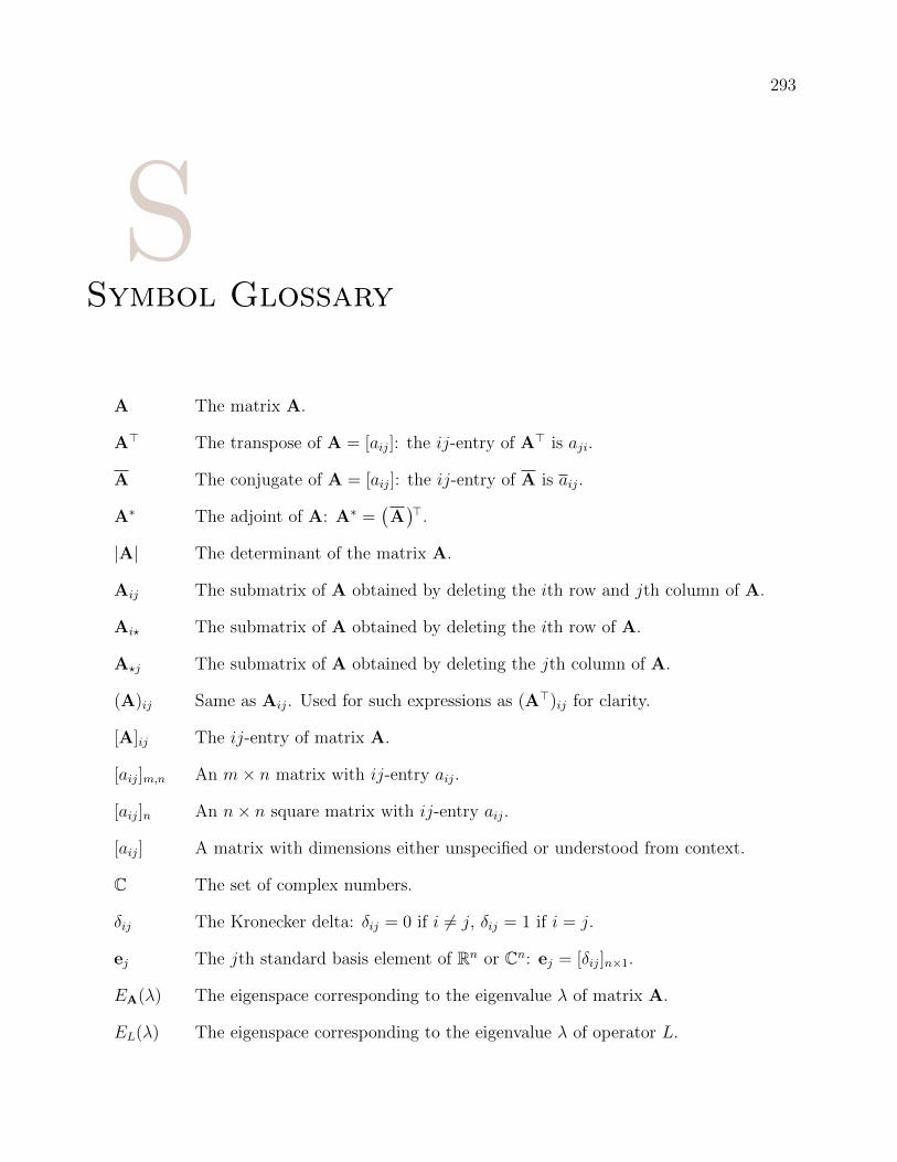
293

SSymbol Glossary

A The matrix A.

A> The transpose of A = [aij]: the ij-entry of A> is aji.

A The conjugate of A = [aij]: the ij-entry of A is aij.

A∗ The adjoint of A: A∗ =(A)>.

|A| The determinant of the matrix A.

Aij The submatrix of A obtained by deleting the ith row and jth column of A.

Ai? The submatrix of A obtained by deleting the ith row of A.

A?j The submatrix of A obtained by deleting the jth column of A.

(A)ij Same as Aij. Used for such expressions as (A>)ij for clarity.

[A]ij The ij-entry of matrix A.

[aij]m,n An m× n matrix with ij-entry aij.

[aij]n An n× n square matrix with ij-entry aij.

[aij] A matrix with dimensions either unspecified or understood from context.

C The set of complex numbers.

δij The Kronecker delta: δij = 0 if i 6= j, δij = 1 if i = j.

ej The jth standard basis element of Rn or Cn: ej = [δij]n×1.

EA(λ) The eigenspace corresponding to the eigenvalue λ of matrix A.

EL(λ) The eigenspace corresponding to the eigenvalue λ of operator L.

294

F An unspecified field, the elements of which are called scalars.

Fn F1×n in Chapter 1, otherwise Fn×1.

Fm×n Set of all m× n matrices with entries in F.

ϕB The coordinate map, where ϕB(v) = [v]B.

γA(λ) The geometric multiplicity of eigenvalue λ of matrix A.

γL(λ) The geometric multiplicity of eigenvalue λ of operator L.

Img(L) Image of linear mapping L : V → W . Img(L) = {L(v) : v ∈ V }.

IBB′ The change of basis matrix from basis B to basis B′.

In The n× n identity matrix.

I An identity matrix, dimensions unspecified or understood from context.

IV The identity operator on vector space V : IV (v) = v for all v ∈ V .

[L] Matrix corresponding to linear mapping L with respect to any basis.

[L]B Matrix corresponding to linear operator L with respect to the basis B.

[L]BC Matrix corresponding to linear mapping L with respect to bases B and C.

L(V ) Image of V under L : V → W . L(V ) = Img(L).

L(V ) Set of all linear operators L : V → V on some vector space V .

L(V,W ) Set of all linear mappings L : V → W on given vector spaces V and W .

µA(λ) The algebraic multiplicity of eigenvalue λ of matrix A.

µL(λ) The algebraic multiplicity of eigenvalue λ of operator L.

Nul(L) Null space of linear mapping L : V → W . Nul(L) = {v ∈ V : L(v) = 0}.

N The set of natural numbers (i.e. positive integers): N = {1, 2, 3, . . .}.

O The zero mapping in L(V,W ): O(v) = 0 for all v ∈ V .

OV The zero operator on vector space V : OV (v) = 0 for all v ∈ V .

0 The zero vector.

F(S,F) The set of all functions S → F.

0V The zero vector of vector space V .

295

Om,n The m× n zero matrix (all entries are 0).

On The n× n zero matrix (all entries are 0).

O A zero matrix, dimensions unspecified or understood from context.

O An orthonormal basis for an inner product space.

Pn(F) The vector space of all polynomials of degree at most n with coefficients in F.

Q The set of rational numbers.

R The set of real numbers.

|S| The number of elements in the set S (i.e. the cardinality of S)

Symn(F) Set of all n× n symmetric matrices with entries in F.

Skwn(F) Set of all n× n skew-symmetric matrices with entries in F.

s∼ The similar matrix relation.

σ(A) Set of all eigenvalues in F of a matrix A ∈ Fn×n.

σ(L) Set of all eigenvalues in F of an operator L ∈ L(V ).

v The vector v.

‖v‖ The norm or magnitude of v; that is, ‖v‖ =√

v · v or ‖v‖ =√〈v,v〉

v The normalization of vector v; that is, v = v/‖v‖

[v]B The B-coordinates of vector v.

W The set of whole numbers: W = {0, 1, 2, 3, . . .}.

Z The set of integers: Z = {1,−1, 2,−2, 3,−3, . . .}.

〈〉 The inner product function.

〈〉V The inner product function of vector space V .

⇒ Symbol for logical implication. Read as “implies” or “implies that.”

⇔ Symbol for logical equivalence. Read as “is equivalent to” or “if and only if.”

linear algebra - bucks county community...

Documents