linear algebra, basic notions 1. introduction example 1.len/linalg/chap1.pdfbasic algebra can get...
TRANSCRIPT

CHAPTER I
LINEAR ALGEBRA, BASIC NOTIONS
1. Introduction
In your previous calculus courses, you studied differentiation and integration forfunctions of more than one variable. Usually, you couldn’t do much if the number ofvariables was greater than two or three. However, in many important applications,the number of relevant variables can be quite large. In such situations, even verybasic algebra can get quite complicated. Linear algebra is a tool invented in thenineteenth century and further extended in the twentieth century to enable peopleto handle such algebra in a systematic and understandable manner.
We start off with a couple of simple examples where it is clear that we may haveto deal with a lot of variables.
Example 1. Professor Marie Curie has ten students in a chemistry class andgives five exams which are weighted differently in order to obtain a total score forthe course. The data as presented in her grade book is as follows.
student/exam 1 2 3 4 51 78 70 74 82 742 81 75 72 85 803 92 90 94 88 944 53 72 65 72 595 81 79 79 82 786 21 92 90 88 957 83 84 76 79 848 62 65 67 73 659 70 72 76 82 7310 69 75 70 78 79
The numbers across the top label the exams and the numbers in the left handcolumn number the students. There are a variety of statistics the teacher mightwant to calculate from this data. First, she might want to know the average scorefor each test. For a given test, label the scores x1, x2, x3, x4, x5, x6, x7, x8, x9, x10
so that xi is the score for the ith student. Then the average score is
x1 + x2 + x2 + x4 + x5 + x6 + x7 + x8 + x9 + x10
10=
110
10∑i=1
xi.
For example, for the second test the average is
110
(70 + 75 + 90 + 72 + 79 + 92 + 84 + 65 + 72 + 75) = 77.4.
1

2 I. LINEAR ALGEBRA, BASIC NOTIONS
Suppose she decides to weight the five scores as follows: the first, third, and fifthscores are weighted equally at 20 percent or 0.2, the second score is weighted 10percent or 0.1, and the fourth score is weighted 30 percent or 0.3. Then if the scoresfor a typical student are denoted y1, y2, y3, y4, y5, the total weighted score would be
0.2 y1 + 0.1 y2 + 0.2 y3 + 0.3 y4 + 0.2 y5.
If we denote the weightings a1 = a3 = a5 = 0.2, a2 = 0.1, a4 = 0.3, then this couldalso be written
a1y1 + a2y2 + a3y3 + a4y4 + a5y5 =5∑
i=1
aiyi.
For example, for the third student, the total score would be
0.2 · 92 + 0.1 · 90 + 0.2 · 94 + 0.3 · 88 + 0.2 · 94 = 91.4.
As you see, in both cases we have a number of variables and we are forming whatis called a linear function of those variables, that is, an expression in which eachvariable appears simply to the first power (with no complicated functions). Whenwe only have two or three variables, the algebra for dealing with such functions isquite simple, but as the number of variables grows, the algebra becomes much morecomplex.
Such data sets and calculations should be familiar to anyone who has playedwith a spreadsheet.
Example 2. In studying complicated electrical circuits, one uses a collection ofrules called Kirchhoff’s laws. One of these rules says that the currents convergingat a node in the circuit add up algebraically to zero. (Currents can be positive ornegative.) Other rules put other restrictions on the currents. For example, in thecircuit below
10
15
10
20
5
50 volts
x 1x 2
x3
5
4
Numerical resistances in ohmsx
x
Kirchhoff’s laws yield the following equations for the currents x1, x2, x3, x4, x5 inthe different branches of the circuit.
10x1 + 10x2 = 5020x3 + 5x4 = 50
x1 − x2 − x5 = 0−x3 + x4 − x5 = 0
10x1 + 5x4 + 15x5 = 50

1. INTRODUCTION 3
Don’t worry if you don’t know anything about electricity. The point is that thecircuit is governed by a system of linear equations. In order to understand thecircuit, we must have methods to solve such systems. In your high school algebracourse, you learned how to solve two equations in two unknowns and perhaps threeequations in three unknowns. In this course we shall study how to solve any numberof equations in any number of unknowns. Linear algebra was invented in large partto discuss the solutions of such systems in an organized manner. The above exampleyielded a fairly small system, but electrical engineers must often deal with verylarge circuits involving many, many currents. Similarly, many other applications inother fields require the solution of systems of very many equations in very manyunknowns.
Nowadays, one uses electronic computers to solve such systems. Consider forexample the system of 5 equations in 5 unknowns
2x1 + 3x2 − 5x3 + 6x4 − x5 = 103x1 − 3x2 + 6x3 + x4 − x5 = 2x1 + x2 − 4x3 + 2x4 + x5 = 5
4x1 − 3x2 + x3 + 6x4 + x5 = 42x1 + 3x2 − 5x3 + 6x4 − x5 = 3
How might you present the data needed to solve this system to a computer? Clearly,the computer won’t care about the names of the unknowns since it doesn’t needsuch aids to do what we tell it to do. It would need to be given the table ofcoefficients
2 3 −5 6 −13 −3 6 1 −11 1 −4 2 14 −3 1 6 12 3 −5 6 −1
and the quantities on the right—also called the ‘givens’
102543
Each such table is an example of a matrix , and in the next section, we shalldiscuss the algebra of such matrices.
Exercises for Section 1.
1. A professor taught a class with three students who took two exams each. Theresults were
student/test 1 21 100 952 60 753 100 95

4 I. LINEAR ALGEBRA, BASIC NOTIONS
(a) What were the average scores on each test?(b) Are there weightings a1, a2 which result in either of the following weighted
scores?student score
1 982 663 98
or
student score1 982 663 97
2. Solve each of the following linear systems by any method you know.(a)
2x + 3y = 3x + 3y = 1
(b)
x + y = 3y + z = 4
x + y + z = 5
(c)
x + y = 3y + z = 4
x + 2y + z = 5
(d)
x + y + z = 1z = 1
2. Matrix Algebra
In the previous section, we saw examples of rectangular arrays or matrices suchas the table of grades
78 70 74 82 7481 75 72 85 8092 90 94 88 9453 72 65 72 5981 79 79 82 7821 92 90 88 9583 84 76 79 8462 65 67 73 6570 72 76 82 7369 75 70 78 79

2. MATRIX ALGEBRA 5
This is called a 10 × 5 matrix. It has 10 rows and 5 columns. More generally, anm× n matrix is a table or rectangular array of the form
a11 a12 . . . a1n
a21 a22 . . . a2n...
... . . ....
am1 am2 . . . amn
It has m rows and n columns. The quantities aij are called the entries of thematrix. They are numbered with subscripts so that the first index i tells you whichrow the entry is in, and the second index j tells you which column it is in.
Examples. [−2 11 −2
]is a 2× 2 matrix
[1 2 3 44 3 2 1
]is a 2× 4 matrix
[x1 x2 x3 x4 ] is a 1× 4 matrix
x1
x2
x3
x4
is a 4× 1 matrix
Matrices of various sizes and shapes arise in applications. For example, everyfinancial spreadsheet involves a matrix, at least implicitly. Similarly, every systemof linear equations has a coefficient matrix.
In computer programming, a matrix is called a 2-dimensional array and the entryin row i and column j is usually denoted a[i, j] instead of aij . As in programming,it is useful to think of the entire array as a single entity, so we use a single letterto denote it
A =
a11 a12 . . . a1n
a21 a22 . . . a2n...
... . . ....
am1 am2 . . . amn
.
There are various different special arrangements which play important roles. Amatrix with the same number of rows as columns is called a square matrix. Matricesof coefficients for systems of linear equations are often square. A 1× 1 matrix
[ a ]
is not logically distinguishable from a number or scalar , so we make no distinctionbetween the two concepts. A matrix with one row
a = [ a1 a2 . . . an ]

6 I. LINEAR ALGEBRA, BASIC NOTIONS
is called a row vector and a matrix with one column
a =
a1
a2...
an
is called a column vector.This terminology requires a bit of explanation. In three dimensional calculus, a
vector is completely determined by its set of components [ v1 v2 v3 ]. Much ofthe analysis you encountered in that subject was simplified by using vector notationv to stand for the vector rather than emphasizing its components. When we wishto generalize to larger numbers of variables, it is also useful to think of a set ofcomponents
[ v1 v2 . . . vn ]
as constituting a higher dimensional vector v. In this way we can use geometricinsights which apply in two or three dimensions to help guide us—by analogy—when discussing these more complicated situations. In so doing, there is a formaldifference between specifying the components horizontally, as above, or verticallyas in
v1
v2...
vn
but logically speaking the same data is specified. In either case, the entity underconsideration should be viewed as a higher dimensional analogue of a vector. Fortechnical reasons which will be clear shortly, we shall usually specify such objectsas column vectors.
Matrices are denoted in different ways by different authors. Most people useordinary (non-boldface) capital letters, e.g., A,B,X,Q. However, one sometimeswants to use boldface for row or column vectors, as above, since boldface is com-monly used for vectors in two and three dimensions and we want to emphasize thatanalogy. Since there are no consistent rules about notation, you should make sureyou know when a symbol represents a matrix which is not a scalar.
Matrices may be combined in various useful ways. Two matrices of the samesize and shape are added by adding corresponding entries. You are not allowed toadd matrices with different shapes.
Examples. 1 −1
2 10 1
+
1 1
0 3−1 −2
=
2 0
2 4−1 −1
x + y
y0
+
−y−yx
=
x
0x
.

2. MATRIX ALGEBRA 7
The m × n matrix with zero entries is called a zero matrix and is usually justdenoted 0. Since zero matrices with different shapes are not the same, it is some-times necessary to indicate the shape by using subscripts, as in ‘0mn’, but usuallythe context makes it clear which zero matrix is needed. The zero matrix of a givenshape has the property that if you add it to any matrix A of the same shape, youget the same A again.
Example. [1 −1 02 3 −2
]+
[0 0 00 0 0
]=
[1 −1 02 3 −2
]
A matrix may also be multiplied by a scalar by multiplying each entry of thematrix by that scalar. More generally, we may multiply several matrices with thesame shape by different scalars and add up the result:
c1A1 + c2A2 + · · ·+ ckAk
where c1, c2, . . . , ck are scalars and A1, A2, . . . , Ak are m×n matrices with the samem and n. This process is called linear combination.
Example.
2
1010
+ (−1)
0101
+ 3
1111
=
2020
+
0−1
0−1
+
3333
=
5252
.
Sometimes it is convenient to put the scalar on the other side of the matrix, butthe meaning is the same: each entry of the matrix is multiplied by the scalar.
cA = Ac.
We shall also have occasion to consider matrix valued functions A(t) of a scalarvariable t. That means that each entry aij(t) is a function of t. Such functions aredifferentiated or integrated entry by entry.
Examples.
d
dt
[e2t e−t
2e2t −e−t
]=
[2e2t −e−t
4e2t e−t
]∫ 1
0
[tt2
]dt =
[1/21/3
]
There are various ways to multiply matrices. For example, one sometimes multi-plies matrices of the same shape by multiplying corresponding entries. This is usefulonly in very special circumstances. Another kind of multiplication generalizes the

8 I. LINEAR ALGEBRA, BASIC NOTIONS
dot product of vectors. In three dimensions, if a has components [ a1 a2 a3 ] andb has components [ b1 b2 b3 ], then the dot product a · b = a1b1 + a2b2 + a3b3;that is, corresponding components are multiplied and the results are added. If
[ a1 a2 . . . an ]
is a row vector of size n, and
b1
b2...
bn
is a column vector of the same size n, the row by column product is defined to bethe sum of the products of corresponding entries
[ a1 a2 . . . an ]
b1
b2...
bn
= a1b1 + a2b2 + · · ·+ anbn =
n∑i=1
aibi.
This product is of course a scalar , and except for the distinction between row andcolumn vectors, it is an obvious generalization of notion of dot product in two orthree dimensions. You should be familiar with its properties.
More generally, let A be an m × n matrix and B an n × p matrix. Then eachrow of A has the same size as each column of B. The matrix product AB is definedto be the m × p matrix with i, j entry the row by column product of the ith rowof A with the jth column of B. Thus, if C = AB, then C has the same number ofrows as A, the same number of columns as B, and
cij =n∑
r=1
airbrj .
Examples. [2 11 0
]︸ ︷︷ ︸
2×2
[1 0 1−1 2 1
]︸ ︷︷ ︸
2×3
=[
2− 1 0 + 2 2 + 11− 0 0 + 0 1 + 0
]︸ ︷︷ ︸
2×3
=[
1 2 31 0 1
] 1 −1
1 02 1
︸ ︷︷ ︸3×2
[xy
]︸︷︷︸2×1
=
x− y
x2x + y
︸ ︷︷ ︸3×1
The most immediate use for matrix multiplication is a simplification of the no-tation used to describe a system of linear equations.

2. MATRIX ALGEBRA 9
Consider the system in the previous section
2x1 + 3x2 − 5x3 + 6x4 − x5 = 103x1 − 3x2 + 6x3 + x4 − x5 = 2x1 + x2 − 4x3 + 2x4 + x5 = 5
4x1 − 3x2 + x3 + 6x4 + x5 = 42x1 + 3x2 − 5x3 + 6x4 − x5 = 3
If you look closely, you will notice that the expressions on the left are the entriesof a matrix product:
2 3 −5 6 −13 −3 6 1 −11 1 −4 2 14 −3 1 6 12 3 −5 6 −1
x1
x2
x3
x4
x5
=
2x1 + 3x2 − 5x3 + 6x4 − x5
3x1 − 3x2 + 6x3 + x4 − x5
x1 + x2 − 4x3 + 2x4 + x5
4x1 − 3x2 + x3 + 6x4 + x5
2x1 + 3x2 − 5x3 + 6x4 − x5
Note that what appears on the right—although it looks rather complicated—is justa 5 × 1 column vector. Thus, the system of equations can be written as a singlematrix equation
2 3 −5 6 −13 −3 6 1 −11 1 −4 2 14 −3 1 6 12 3 −5 6 −1
x1
x2
x3
x4
x5
=
102543
.
If we use the notation
A =
2 3 −5 6 −13 −3 6 1 −11 1 −4 2 14 −3 1 6 12 3 −5 6 −1
, x =
x1
x2
x3
x4
x5
b =
102543
,
then the system can be written even more compactly
Ax = b.
Of course, this notational simplicity hides a lot of real complexity, but it does helpus to think about the essentials of the problem.
More generally, an arbitrary system of m equations in n unknowns has the form
a11 a12 . . . a1n
a21 a22 . . . a2n...
... . . ....
am1 am2 . . . amn
x1
x2...
xn
=
b1
b2...
bm
,

10 I. LINEAR ALGEBRA, BASIC NOTIONS
where
A =
a11 a12 . . . a1n
a21 a22 . . . a2n...
... . . ....
am1 am2 . . . amn
is the coefficient matrix and
x =
x1
x2...
xn
and b =
b1
b2...
bm
,
are column vectors of unknowns and ‘givens’ respectively.Later in this chapter, we shall investigate systematic methods for solving systems
of linear equations.
Special Operations for Row or Column Vectors. We have already re-marked that a column vector
v =
v1
v2...
vn
may be viewed as a generalization of a vector in two or three dimensions. We alsoused a generalization of the dot product of two such vectors in defining the matrixproduct. In a similar fashion, we may define the length of a row vector or columnvector to be the square root of the sum of the squares of its components. Forexample. for
v =
12
−34
, we have |v| =
√12 + 22 + (−3)2 + 42 =
√30.
Exercises for Section 2.
1. Let
x =
1
2−3
, y =
−2
13
, z =
1
0−1
.
Calculate x + y and 3x− 5y + z.
2. Let
A =
2 7 4 −3−3 0 1 −2
1 3 −2 30 0 5 −5
, x =
1−2
35
, y =
−2
204
.
Compute Ax, Ay, Ax + Ay, and A(x + y).

2. MATRIX ALGEBRA 11
3. Let
A =[
1 −1 30 −2 2
], B =
1 2
1 0−3 2
, C =
[−1 1 −30 2 −2
], D =
−1 −2 0
1 −2 12 1 −4
.
Calculate each of the following quantities if it is defined : A + 3B, A + C, C +2D, AB,BA,CD,DC.
4. Suppose A is a 2× 2 matrix such that
A
[12
]=
[31
]A
[21
]=
[64
].
Find A.
5. Let ei denote the n × 1 column vector, with all entries zero except the ithwhich is 1, e.g., for n = 3,
e1 =
1
00
, e2 =
0
10
, e3 =
0
01
.
Let A be an arbitrary m × n matrix. Show that Aei is the ith column of A. Youmay verify this just in the case n = 3 and A is 3× 3. That is sufficiently general tounderstand the general argument.
6. Write each of the following systems in matrix form.(a)
2x1 − 3x2 = 2−4x1 + 2x2 = 3
(b)
2x1 − 3x2 = 4−4x1 + 2x2 = 1
(c)
x1 + x2 = 1x2 + x3 = 1
2x1 + 3x2 − x3 = 0
7. (a) Determine the lengths of the following column vectors
u =
12−21
,v =
100−1
,w =
0220
.
(b) Are any of these vectors mutually perpendicular?(c) Find unit vectors proportional to each of these vectors.

12 I. LINEAR ALGEBRA, BASIC NOTIONS
8. One kind of magic square is a square array of numbers such that the sum ofevery row and the sum of every column is the same number.
(a) Which of the following matrices present magic squares?
[1 34 2
] 1 2 1
2 1 11 1 2
(b) Use matrix multiplication to describe the condition that an n× n matrix Apresents a magic square.
9. Population is often described by a first order differential equation of the formdp
dt= rp where p represents the population and r is a parameter called the growth
rate. However, real populations are more complicated. For example, human pop-ulations come in different ages with different fertility. Matrices are used to createmore realistic population models. Here is an example of how that might be done
Assume a human population is divided into 10 age groups between 0 and 99.Let xi, i = 1, 2, . . . , 10 be the number of women in the ith age group, and considerthe vector x with those components. (For the sake of this exercise, we ignore men.)Suppose the following table gives the birth and death rates for each age group ineach ten year period.
i Age BR DR1 0 . . . 9 0 .012 10 . . . 19 .01 .013 20 . . . 29 .04 .014 30 . . . 39 .03 .015 40 . . . 49 .01 .026 50 . . . 59 .001 .037 60 . . . 69 0 .048 70 . . . 79 0 .109 80 . . . 89 0 .30
10 90 . . . 99 0 1.00
For example, the fourth age group is women age 30 to 39. In a ten year period, weexpect this group to give birth to .03x4 girls, all of whom will be in the first agegroup at the beginning of the next ten year period. We also expect .01x4 of themto die, which tells us something about the value of x5 at the beginning of the nextten year period.
Construct a 10 × 10 matrix A which incorporates this information about birthand death rates so that Ax gives the population vector after one ten year periodhas elapsed.
Note that Anx keeps track of the population structure after n ten year periodshave elapsed.

3. FORMAL RULES 13
3. Formal Rules
The usual rules of algebra apply to matrices with a few exceptions. Here aresome of these rules and warnings about when they apply.
The associative lawA(BC) = (AB)C
works as long as the shapes of the matrices match. That means that the length ofeach row of A must be the same as the length of each column of B and the lengthof each row of B must be the same as the length of each column of C. Otherwise,none of the products in the formula will be defined.
Example 1. Let
A =[
1 0−1 1
], B =
[1 1 21 −1 0
], C =
3
21
.
Then
AB =[
1 1 20 −2 −2
], (AB)C =
[7−6
],
while
BC =[
71
], A(BC) =
[1 0−1 1
] [71
]=
[7−6
].
Note that this is bit more complicated than the associative law for ordinary numbers(scalars).
For those who are interested, the proof of the general associative law is outlinedin the exercises.
For each positive integer n, the n× n matrix
I =
1 0 . . . 00 1 . . . 0...
... . . ....
0 0 . . . 1
is called the identity matrix of degree n. As in the case of the zero matrices, weget a different identity matrix for each n, and if we need to note the dependence onn, we shall use the notation In. The identity matrix of degree n has the propertyIA = A for any matrix A with n rows and the property BI = B for any matrix Bwith n columns.
Example 2. Let
I =
1 0 0
0 1 00 0 1
be the 3× 3 identity matrix. Then, for example, 1 0 0
0 1 00 0 1
1 3
4 2−1 6
=
1 3
4 2−1 6

14 I. LINEAR ALGEBRA, BASIC NOTIONS
and [1 2 33 2 1
] 1 0 0
0 1 00 0 1
=
[1 2 33 2 1
].
The entries of the identity matrix are usually denoted δij . δij = 1 if i = j (thediagonal entries) and δij = 0 if i 6= j. The indexed expression δij is often calledthe Kronecker δ.
The commutative law AB = BA is not generally true for matrix multiplication.First of all, the products won’t be defined unless the shapes match. Even if theshapes match on both sides, the resulting products may have different sizes. Thus,if A is m × n and B is n ×m, then AB is m ×m and BA is n × n. Finally, evenif the shapes match and the products have the same sizes (if both A and B aren× n), it may still be true that the products are different.
Example 3. Suppose
A =[
1 00 0
]B =
[0 01 0
].
Then
AB =[
0 00 0
]= 0 BA =
[0 01 0
]6= 0
so AB 6= BA. Lest you think that this is a specially concocted example, let meassure you that it is the exception rather than the rule for the commutative law tohold for a randomly chosen pair of square matrices.
Another rule of algebra which holds for scalars but does not generally hold formatrices is the cancellation law.
Example 4. Let
A =[
1 00 0
]B =
[0 01 0
]C =
[0 00 1
].
ThenAB = 0 and AC = 0
so we cannot necessarily conclude from AB = AC that B = C.
The distributive laws
A(B + C) = AB + AC
(A + B)C = AC + BC
do hold as long as the operations are defined. Note however that since the com-mutative law does not hold in general, the distributive law must be stated for bothpossible orders of multiplication.
Another useful rule is
c(AB) = (cA)B = A(cB)

4. LINEAR SYSTEMS OF ALGEBRAIC EQUATIONS 15
where c is a scalar and A and B are matrices whose shapes match so the productsare defined.
The rules of calculus apply in general to matrix valued functions except that youhave to be careful about orders whenever products are involved. For example, wehave
d
dt(A(t)B(t)) =
dA(t)dt
B(t) + A(t)dB(t)
dt
for matrix valued functions A(t) and B(t) with matching shapes.We have just listed some of the rules of algebra and calculus, and we haven’t
discussed any of the proofs. Generally, you can be confident that matrices canbe manipulated like scalars if you are careful about matters like commutativitydiscussed above. However, in any given case, if things don’t seem to be workingproperly, you should look carefully to see if some operation you are using is validfor matrices.
Exercises for Section 3.
1. (a) Let I be the 3× 3 identity matrix. What is I2? How about I3, I4, I5, etc.?
(b) Let J =[
0 11 0
]. What is J2?
2. Find two 2 × 2 matrices A and B such that neither has any zero entries butsuch that AB = 0.
3. Let A be an m× n matrix, let x and y be n× 1 column vectors, and let a andb be scalars. Using the rules of algebra discussed in Section 3, prove
A(ax + by) = a(Ax) + b(Ay).
4. (Optional) Prove the associative law (AB)C = A(BC). Hint: If D = AB,then dik =
∑nj=1 aijbjk, and if E = BC then ejr =
∑pk=1 bjkckr, where A is m×n,
B is n× p, and C is p× q.
5. Verify the following relation
d
dt
[cos t − sin tsin t cos t
]=
[0 −11 0
] [cos t − sin tsin t cos t
].
4. Linear Systems of Algebraic Equations
We start with a problem you ought to be able to solve from what you learned inhigh school
Example 1. Consider the algebraic system
(1)
x1 + 2x2 − x3 = 1x1 − x2 + x3 = 0
x1 + x2 + 2x3 = 1

16 I. LINEAR ALGEBRA, BASIC NOTIONS
which is a system of 3 equations in 3 unknowns x1, x2, x3. This system may alsobe written more compactly as a matrix equation
1 2 −11 −1 11 1 2
x1
x2
x3
=
1
01
.
The method we shall use to solve (1) is the method of elimination of unknowns.Subtract the first equation from each of the other equations to eliminate x1 fromthose equations.
x1 + 2x2 − x3 = 1−3x2 + 2x3 = −1−x2 + 3x3 = 0
Now subtract 3 times the third equation from the second equation.
x1 + 2x2 − x3 = 1−7x3 = −1
−x2 + 3x3 = 0
which may be reordered to obtain
x1 + 2x2 − x3 = 1−x2 + 3x3 = 0
7x3 = 1.
We may now solve as follows. According to the last equation x3 = 1/7. Puttingthis in the second equation yields
−x2 + 3/7 = 0 or x2 = 3/7.
Putting x3 = 1/7 and x2 = 3/7 in the first equation yields
x1 + 2(3/7)− 1/7 = 1 or x1 = 1− 5/7 = 2/7.
Hence, we get
x1 = 2/7
x2 = 3/7
x3 = 1/7
To check, we calculate 1 2 −1
1 −1 11 1 2
2/7
3/71/7
=
1
01
.

4. LINEAR SYSTEMS OF ALGEBRAIC EQUATIONS 17
The above example illustrates the general procedure which may be applied toany system of m equations in n unknowns
a11x1 + a12x2 + · · ·+ a1nxn = b1
a21x1 + a22x2 + · · ·+ a2nxn = b2
...am1x1 + am2x2 + · · ·+ amnxn = bm
or, using matrix notation,Ax = b
with
A =
a11 a12 . . . a1n
a21 a22 . . . a2n...
... . . ....
am1 am2 . . . amn
x =
x1
x2...
xn
b =
b1
b2...
bm
.
As in Example 1, a sequence of elimination steps yields a set of equations eachinvolving at least one fewer unknowns than the one above it. This process is calledGaussian reduction after the famous 19th century German mathematician C. F.Gauss. To complete the solution, we start with the last equation and substitute backrecursively in each of the previous equations. This process is called appropriatelyback-substitution. The combined process will generally lead to a complete solution,but, as we shall see later, there can be some difficulties.
Row Operations and Gauss-Jordan reduction. Generally a system of mequations in n unknowns can be written in matrix form
Ax = b
where A is an m×n matrix of coefficients, x is a n× 1 column vector of unknownsand b is a m× 1 column vector of givens. It turns out to be just about as easy tostudy more general systems of the form
AX = B

18 I. LINEAR ALGEBRA, BASIC NOTIONS
where A is an m× n matrix, X is an n× p matrix of unknowns, and B is a knownm × p matrix. Usually, p will be 1, so X and B will be column vectors, but theprocedure is basically the same for any p. For the moment we emphasize the casein which the coefficient matrix A is square, i.e., m = n, but we shall return later tothe general case (m and n possibly different).
If you look carefully at Example 1, you will see that we employed three basictypes of operations:
(1) adding or subtracting a multiple of one equation from another,(2) multiplying or dividing an equation by a non-zero scalar,(3) interchanging two equations.
Translated into matrix notation, these operations correspond to applying thefollowing operations to the matrices on both sides of the equation AX = B:
(1) adding or subtracting one row of a matrix to another,(2) multiplying or dividing one row of a matrix by a non-zero scalar,(3) interchanging two rows of a matrix.
(The rows of the matrices correspond to the equations.)These operations are called elementary row operations.An important principle about row operations that we shall use over and over
again is the following: To apply a row operation to a product AX, it suffices toapply the row operation to A and then to multiply the result by X. It is easy toconvince yourself that this rule is valid by looking at examples.
Example. Suppose
A =[
1 32 4
], X =
[1 2 33 2 1
].
Apply the operation of adding −2 times the first row of A to the second row of A.[1 32 4
]→
[1 30 −2
]
and multiply by X to get[1 30 −2
] [1 2 33 2 1
]=
[10 8 6−6 −4 −2
].
On the other hand, first compute
AX =[
1 32 4
] [1 2 33 2 1
]=
[10 8 614 12 10
]
and then add −2 times its first row to its second row to obtain[10 8 614 10 12
]→
[10 8 6−6 −4 −2
].
Note that the result is the same by either route.

4. LINEAR SYSTEMS OF ALGEBRAIC EQUATIONS 19
If you want to see a general explanation of why this works, see the appendix tothis section.
This suggests a procedure for solving a system of the form
AX = B.
Apply row operations to both sides until we obtain a system which is easy tosolve (or for which it is clear there is no solution.) Because of the principle justenunciated, we may apply the row operations on the left just to the matrix A andomit reference to X since that is not changed. For this reason, it is usual to collectA on the left and B on the right in a so-called augmented matrix
[A |B]
where the ‘|’ (or other appropriate divider) separates the two matrices. We illustratethis by redoing Example 1, but this time using matrix notation.
Example 1, redone. The system was
x1 + 2x2 − x3 = 1x1 − x2 + x3 = 0
x1 + x2 + 2x3 = 1
so the augmented matrix is 1 2 −1 | 1
1 −1 1 | 01 1 2 | 1
We first do the Gaussian part of the reduction using row operations. The rowoperations are indicated to the right with the rows that are changed in bold face.
1 2 −1 | 11 −1 1 | 01 1 2 | 1
→
1 2 −1 | 1
0 −3 2 | −11 1 2 | 1
− 1[row1] + row2
→ 1 2 −1 | 1
0 −3 2 | −10 −1 3 | 0
− 1[row1] + row3
→ 1 2 −1 | 1
0 0 −7 | −10 −1 3 | 0
− 3[row3] + row2
→ 1 2 −1 | 1
0 −1 3 | 00 0 −7 | −1
row3 ↔ row2
Compare this with the previous reduction using equations. We can reconstruct thecorresponding system from the augmented matrix, and, as before, we get
x1 + 2x2 − x3 = 1−x2 + 3x3 = 0
−7x3 = −1

20 I. LINEAR ALGEBRA, BASIC NOTIONS
Earlier, we applied back-substitution to find the solution. However, it is betterfor matrix computation to use an essentially equivalent process. Starting with thelast row, use the leading non-zero entry to eliminate the entries above it. (Thatcorresponds to substituting the value of the corresponding unknown in the previousequations.) This process is called Jordan reduction. The combined process is calledGauss–Jordan reduction. or, sometimes, reduction to row reduced echelon form.
1 2 −1 | 1
0 −1 3 | 00 0 −7 | −1
→
1 2 −1 | 1
0 −1 3 | 00 0 1 | 1/7
(1/7)[row3]
→ 1 2 −1 | 1
0 −1 0 | −3/70 0 1 | 1/7
− 3[row3] + row2
→ 1 2 0 | 8/7
0 −1 0 | −3/70 0 1 | 1/7
[row3] + row1
→ 1 0 0 | 2/7
0 −1 0 | −3/70 0 1 | 1/7
2[row2] + row1
→ 1 0 0 | 2/7
0 1 0 | 3/70 0 1 | 1/7
− 1[row2]
This corresponds to the system
1 0 0
0 1 00 0 1
X =
2/7−3/7
1/7
or X = IX =
2/7−3/7
1/7
which is the desired solution: x1 = 2/7, x2 = −3/7, x3 = 1/7.
Here is another similar example.
Example 2.
x1 + x2 − x3 = 02x1 + x3 = 2x1 − x2 + 3x3 = 1
or
1 1 −1
2 0 11 −1 3
x1
x2
x2
=
0
21

4. LINEAR SYSTEMS OF ALGEBRAIC EQUATIONS 21
Reduce the augmented matrix as follows. 1 1 −1 | 0
2 0 1 | 21 −1 3 | 1
→
1 1 −1 | 0
0 −2 3 | 21 −1 3 | 1
− 2[r1] + [r2]
→ 1 1 −1 | 0
0 −2 3 | 20 −2 4 | 1
− [r1] + [r3]
→ 1 1 −1 | 0
0 −2 3 | 20 0 1 | −1
− [r2] + [r3]
This completes the Gaussian reduction. Now continue with the Jordan reduction. 1 1 −1 | 0
0 −2 3 | 20 0 1 | −1
→
1 1 −1 | 0
0 −2 0 | 50 0 1 | −1
− 3[r3] + [r2]
→ 1 1 0 | −1
0 −2 0 | 50 0 1 | −1
[r3] + [r1]
→ 1 1 0 | −1
0 1 0 | −5/20 0 1 | −1
− (1/2)[r2]
→ 1 0 0 | −3/2
0 1 0 | −5/20 0 1 | −1
− [r2] + [r1]
This corresponds to the system 1 0 0
0 1 00 0 1
X =
−3/2−5/2−1
or X = IX =
−3/2−5/2−1
which is the desired solution: x1 = −3/2, x2 = −5/2, x3 = −1. (Check it byplugging back into the original matrix equation.)
The strategy is clear. Use the sequence of row operations as indicated aboveto reduce the coefficient matrix A to the identity matrix I. If this is possible, thesame sequence of row operations will transform the matrix B to a new matrix B′,and the corresponding matrix equation will be
IX = B′ or X = B′.
It is natural at this point to conclude that X = B′ is the solution of the originalsystem, but there is a subtle problem with that. As you may have learned in highschool, the process of solving an equation or a system of equations may introduceextraneous solutions. These are not actually solutions of the original equations,

22 I. LINEAR ALGEBRA, BASIC NOTIONS
but are introduced by some algebraic manipulation along the way. In particular, itmight be true that the original system AX = B has no solutions, and the conclusionX = B′ is an artifact of the process. The best we conclude from the above logicis the following: if there is a solution, and if it is possible to reduce A to I by asequence of row operations, then the solution is X = B′. That is, if a solutionexists, it is unique, i.e., there is only one solution. To see that the solution mustbe unique, argue as follows. Suppose there were two solutions X and Y . Then wewould have
AX = B
AY = B.
Subtraction would then yield
A(X − Y ) = 0 or AZ = 0 where Z = X − Y.
However, we could apply our sequence of row operations to the equation AZ = 0to obtain IZ = 0 since row operations have no effect on the zero matrix. Thus, wewould conclude that Z = X − Y = 0 or X = Y .
How about the question of whether or not there is a solution in the first place?Of course, in any given case, we can simply check that X = B′ is a solution bysubstituting B′ for X in AX = B and seeing that it works. However, this relies onknowing A and B explicitly. So, it would be helpful if we had a general argumentwhich assured us that X = B′ is a solution when the reduction is possible. (Amongother things, we could skip the checking process if we were sure we did all thearithmetic correctly.)
To understand why X = B′ definitely is a solution, we need another argument.First note that every possible row operation is reversible. Thus, to reverse the effectof adding a multiple of one row to another, just subtract the same multiple of thefirst row from the (modified) second row. To reverse the effect of multiplying arow by a non-zero scalar, just multiply the (modified) row by the reciprocal of thatscalar. Finally, to reverse the effect of interchanging two rows, just interchange themback. Hence, the effect of any sequence of row operations on a system of equationsis to produce an equivalent system of equations. Anything which is a solution ofthe initial system is necessarily a solution of the transformed system and vice-versa.Thus, the system AX = B is equivalent to the system X = IX = B′, which is tosay X = B′ is a solution of AX = B.
Appendix. Elementary Matrices and the Effect of Row Operationson Products. Each of the elementary row operations may be accomplished bymultiplying by an appropriate square matrix on the left. Such matrices of courseshould have the proper size for the matrix being multiplied.
To add c times the jth row of a matrix to the ith row (with i 6= j), multiplythat matrix on the left by the matrix Eij(c) which has diagonal entries 1, the i, j-entry c, and all other entries 0. This matrix may also be obtained by applying thespecified row operation to the identity matrix. You should try out a few examplesto convince yourself that it works.
4. LINEAR SYSTEMS OF ALGEBRAIC EQUATIONS 23
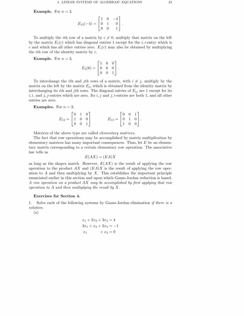
Example. For n = 3,
E13(−4) =
1 0 −4
0 1 00 0 1
.
To multiply the ith row of a matrix by c 6= 0, multiply that matrix on the leftby the matrix Ei(c) which has diagonal entries 1 except for the i, i-entry which isc and which has all other entries zero. Ei(c) may also be obtained by multiplyingthe ith row of the identity matrix by c.
Example. For n = 3,
E2(6) =
1 0 0
0 6 00 0 1
.
To interchange the ith and jth rows of a matrix, with i 6= j, multiply by thematrix on the left by the matrix Eij which is obtained from the identity matrix byinterchanging its ith and jth rows. The diagonal entries of Eij are 1 except for itsi, i, and j, j-entries which are zero. Its i, j and j, i-entries are both 1, and all otherentries are zero.
Examples. For n = 3,
E12 =
0 1 0
1 0 00 0 1
E13 =
0 0 1
0 1 01 0 0
.
Matrices of the above type are called elementary matrices.The fact that row operations may be accomplished by matrix multiplication by
elementary matrices has many important consequences. Thus, let E be an elemen-tary matrix corresponding to a certain elementary row operation. The associativelaw tells us
E(AX) = (EA)X
as long as the shapes match. However, E(AX) is the result of applying the rowoperation to the product AX and (EA)X is the result of applying the row oper-ation to A and then multiplying by X. This establishes the important principleenunciated earlier in this section and upon which Gauss-Jordan reduction is based.A row operation on a product AX may be accomplished by first applying that rowoperation to A and then multiplying the result by X.
Exercises for Section 4.
1. Solve each of the following systems by Gauss-Jordan elimination if there is asolution.
(a)
x1 + 2x2 + 3x3 = 43x1 + x2 + 2x3 = −1x1 + x3 = 0

24 I. LINEAR ALGEBRA, BASIC NOTIONS
(b)
x1 + 2x2 + 3x3 = 42x1 + 3x2 + 2x3 = −1
x1 + x2 − x3 = 10
(c)
1 1 −2 32 1 0 11 −1 1 03 1 2 1
x1
x2
x3
x4
=
9−18−9
9
.
2. Use Gaussian elimination to solve
[3 22 1
]X =
[0 11 0
]
where X is an unknown 2× 2 matrix.
3. Solve each of the following matrix equations
(a)[
1 21 2
]X =
[0 11 0
](b)
1 0 1
0 1 11 1 0
X =
1 0
0 12 1
4. What is the effect of multiplying a 2× 2 matrix A on the right by the matrix
E =[
1 a0 1
]?
What general rule is this a special case of? (E is a special case of an elementarymatrix, as discussed in the Appendix.)
5. (Optional) Review the material in the Appendix on elementary matrices. Thencalculate
1 0 1
0 1 00 0 1
1 0 0−1 1 0
0 0 1
0 1 0
1 0 00 0 1
2 0 0
0 1 00 0 1
1 2 3
4 5 67 8 9
.
Hint: Use the row operations suggested by the first four matrices.

5. SINGULARITY, PIVOTS, AND INVERTIBLE MATRICES 25
5. Singularity, Pivots, and Invertible Matrices
Let A be a square coefficient matrix. Gauss-Jordan reduction will work as in-dicated in the previous section if A can be reduced by a sequence of elementaryrow operations to the identity matrix I. A square matrix with this property iscalled non-singular or invertible. (The reason for the latter terminology will beclear shortly.) If it cannot be so reduced, it is called singular. Clearly, there aresingular matrices. For example, the matrix equation[
1 11 1
] [x1
x2
]=
[10
]
is equivalent to the system of 2 equations in 2 unknowns
x1 + x2 = 1x1 + x2 = 0
which is inconsistent and has no solution. Thus Gauss-Jordan reduction certainlycan’t work on its coefficient matrix.
To understand how to tell if a square matrix A is non-singular or not, we lookmore closely at the Gauss-Jordan reduction process. The basic strategy is thefollowing. Start with the first row, and use type (1) row operations to eliminate allentries in the first column below the 1, 1-position. A leading non-zero entry of arow, when used in this way, is called a pivot. There is one problem with this courseof action: the leading non-zero entry in the first row may not be in the 1, 1-position.In that case, first interchange the first row with a succeeding row which does havea non-zero entry in the first column. (If you think about it, you may still see aproblem. We shall come back to this and related issues later.)
After the first reduction, the coefficient matrix will have been transformed to amatrix of the form
p1 ∗ . . . ∗0 ∗ . . . ∗...
... . . ....
0 ∗ . . . ∗
where p1 is the (first) pivot. We now do something mathematicians (and computerscientists) love: repeat the same process for the submatrix consisting of the secondand subsequent rows. If we are fortunate, we will be able to transform A ultimatelyby a sequence of elementary row operations into matrix of the form
p1 ∗ ∗ . . . ∗0 p2 ∗ . . . ∗0 0 p3 . . . ∗...
...... . . .
...0 0 0 . . . pn
with pivots on the diagonal and nonzero-entries in those pivot positions. (Such amatrix is also called an upper triangular matrix because it has zeroes below the

26 I. LINEAR ALGEBRA, BASIC NOTIONS
diagonal.) If we get this far, we are bound to succeed. Start in the lower right handcorner and apply the Jordan reduction process. In this way each entry above thepivots on the diagonal may be eliminated. We obtain this way a diagonal matrix
p1 0 0 . . . 00 p2 0 . . . 00 0 p3 . . . 0...
...... . . .
...0 0 0 . . . pn
with non-zero entries on the diagonal. We may now finish off the process by applyingtype (2) operations to the rows as needed and finally obtain the identity matrix Ias required.
The above analysis makes clear that the placement of the pivots is what isessential to non-singularity. What can go wrong? Let’s look at an example.
Example 1. 1 2 −1
1 2 01 2 −2
→
1 2 −1
0 0 10 0 −1
clear 1st column
→ 1 2 0
0 0 10 0 0
no pivot in 2, 2 position
Note that the last row consists of zeroes.
The general case is similar. It may happen for a given row that the leadingnon-zero entry is not in the diagonal position, and there is no way to remedy thisby interchanging with a subsequent row. In that case, we just do the best we can.We use a pivot as far to the left as possible (after suitable row interchange with asubsequent row where necessary). In the extreme case, it may turn out that thesubmatrix we are working with consists only of zeroes, and there are no possiblepivots to choose, so we stop. For a singular square matrix, this extreme case mustoccur, since we will run out of pivot positions before we run out of rows. Thus,the Gaussian reduction will still transform A to an upper triangular matrix A′, butsome of the diagonal entries will be zero and some of the last rows (perhaps onlythe last row) will consist of zeroes. That is the singular case.
We showed in the previous section that if the n × n matrix A is non-singular,then every equation of the form AX = B (where both X and B are n×p matrices)does have a solution and also that the solution X = B′ is unique. On the otherhand, if A is singular , an equation of the form AX = B may have a solution, butthere will certainly be matrices B for which AX = B has no solutions. This is bestillustrated by an example.
Example 2. Consider the system 1 2 −1
1 2 01 2 −2
x = b

5. SINGULARITY, PIVOTS, AND INVERTIBLE MATRICES 27
where x and b are 3 × 1 column vectors. Without specifying b, the reduction ofthe augmented matrix for this system would follow the scheme
1 2 −1 | b1
1 2 0 | b2
1 2 −2 | b3
→
1 2 −1 | ∗
0 0 1 | ∗0 0 −1 | ∗
→
1 2 0 | b′1
0 0 1 | b′20 0 0 | b′3
.
Now simply choose b′3 = 1 (or any other non-zero value), so the reduced system isinconsistent. (Its last equation would be 0 = b′3 6= 0.) Since, the two row operationsmay be reversed, we can now work back to a system with the original coefficientmatrix which is also inconsistent. (Check in this case that if you choose b′1 = 0, b′2 =1, b′3 = 1, then reversing the operations yields b1 = −1, b2 = 0, b3 = −1.)
The general case is completely analogous. Suppose
A → · · · → A′
is a sequence of elementary row operations which transforms A to a matrix A′ forwhich the last row consists of zeroes. Choose any n × p matrix B′ for which thelast row does not consist of zeroes. Then the equation
A′X = B′
cannot be valid since the last row on the left will necessarily consist of zeroes. Nowreverse the row operations in the sequence which transformed A to A′. Let B bethe effect of this reverse sequence on B′.
A ← · · · ← A′
B ← · · · ← B′
Then the equationAX = B
cannot be consistent because the equivalent system A′X = B′ is not consistent.We shall see later that when A is a singular n × n matrix, if AX = B has a
solution X for a particular B, then it has infinitely many solutions.There is one unpleasant possibility we never mentioned. It is conceivable that
the standard sequence of elementary row operations transforms A to the identitymatrix, so we decide it is non-singular, but some other bizarre sequence of elemen-tary row operations transforms it to a matrix with some rows consisting of zeroes,in which case we should decide it is singular. Fortunately this can never happenbecause singular matrices and non-singular matrices have diametrically opposedproperties. For example, if A is non-singular then AX = B has a solution for everyB, while if A is singular, there are many B for which AX = B has no solution.This fact does not depend on the method we use to find solutions.
Inverses of Non-singular Matrices. Let A be a non-singular n× n matrix.According to the above analysis, the equation
AX = I
(where we take B to be the n × n identity matrix I) has a unique n × n solutionmatrix X = B′. This B′ is called the inverse of A, and it is usually denoted A−1.That explains why non-singular matrices are also called invertible.

28 I. LINEAR ALGEBRA, BASIC NOTIONS
Example 3. Consider
A =
1 0 −1
1 1 01 2 0
To solve AX = I, we reduce the augmented matrix [A | I]. 1 0 −1 | 1 0 0
1 1 0 | 0 1 01 2 0 | 0 0 1
→
1 0 −1 | 1 0 0
0 1 1 | −1 1 00 2 1 | −1 0 1
→ 1 0 −1 | 1 0 0
0 1 1 | −1 1 00 0 −1 | 1 −2 1
→ 1 0 −1 | 1 0 0
0 1 1 | −1 1 00 0 1 | −1 2 −1
→ 1 0 0 | 0 2 −1
0 1 0 | 0 −1 10 0 1 | −1 2 −1
.
(You should make sure you see which row operations were used in each step.) Thus,the solution is
X = A−1 =
0 2 −1
0 −1 1−1 2 −1
.
Check the answer by calculating
A−1A =
0 2 −1
0 −1 1−1 2 −1
1 0 −1
1 1 01 2 0
=
1 0 0
0 1 00 0 1
.
There is a subtle point about the above calculations. The matrix inverse X =A−1 was derived as the unique solution of the equation AX = I, but we checked itby calculating A−1A = I. The definition of A−1 told us only that AA−1 = I. Sincematrix multiplication is not generally commutative, how could we be sure that theproduct in the other order would also be the identity I? The answer is providedby the following tricky argument. Let Y = A−1A. Then
AY = A(A−1A) = (AA−1)A = IA = A
so that Y is the unique solution of the equation AY = A. However, Y = I is alsoa solution of that equation, so we may conclude that A−1A = Y = I. The upshotis that for a non-singular square matrix A, we have both AA−1 = I and A−1A = I.
The existence of matrix inverses for non-singular square matrices suggests thefollowing scheme for solving matrix equations of the form
AX = B.

5. SINGULARITY, PIVOTS, AND INVERTIBLE MATRICES 29
First, find the matrix inverse A−1, and then take X = A−1B. This is indeed thesolution since
AX = A(A−1B) = (AA−1)B = IB = B.
However, as easy as this looks, one should not be misled by the formal algebra. Theonly method we have for finding the matrix inverse is to apply Gauss-Jordan reduc-tion to the augmented matrix [A | I]. If B has fewer than n columns, then applyingGauss-Jordan reduction directly to [A |B] would ordinarily involve less computa-tion that finding A−1. Hence, it is usually the case that applying Gauss-Jordanreduction to the original system of equations is the best strategy. An exceptionto this rule is where we have one common coefficient matrix A and many differentmatrices B, or perhaps a B with a very large number of columns. In that case, itseems as though it would make sense to find A−1 first. However, there is a varia-tion of Gauss-Jordan reduction called the LU decomposition, that is more efficientand avoids the necessity for calculating the inverse and multiplying by it. See theappendix to this section for a brief discussion of the LU decomposition.
A Note on Strategy. The methods outlined in this and the previous sectioncall for us first to reduce the coefficient matrix to one with zeroes below the diagonaland pivots on the diagonal. Then, starting in the lower right hand corner , we useeach pivot to eliminate the non-zero entries in the column above the pivot. Whyis it important to start at the lower right and work backwards? For that matter,why not just clear each column above and below the pivot as we go? There is avery good reason for that. We want to do as little arithmetic as possible. If weclear the column above the rightmost pivot first, then nothing we do subsequentlywill affect the entries in that column. Doing it in some other order would requirelots of unnecessary arithmetic in that column. For a system with two or threeunknowns, this makes little difference. However, for large systems, the number ofoperations saved can be considerable. Issues like this are specially important indesigning computer algorithms for solving systems of equations.
Numerical Considerations in Computation. The examples we have chosento illustrate the principles employ small matrices for which one may do exact arith-metic. The worst that will happen is that some of the fractions may get a bit messy.In real applications, the matrices are often quite large, and it is not practical todo exact arithmetic. The introduction of rounding and similar numerical approx-imations complicates the situation, and computer programs for solving systems ofequations have to deal with problems which arise from this. If one is not carefulin designing such a program, one can easily generate answers which are very faroff, and even deciding when an answer is sufficiently accurate sometimes involvesrather subtle considerations. Typically, one encounters problems for matrices inwhich the entries differ radically in size. Also, because of rounding, few matricesare ever exactly singular since one can never be sure that a very small numericalvalue at a potential pivot would have been zero if the calculations had been doneexactly. On the other hand, it is not surprising that matrices which are close tobeing singular can give computer programs indigestion.
In practical problems on a computer, the organization and storage of data canalso be quite important. For example, it is usually not necessary to keep the old

30 I. LINEAR ALGEBRA, BASIC NOTIONS
entries as the reduction proceeds. It is important, however, to keep track of therow operations. The memory locations which become zero in the reduction processare ideally suited for storing the relevant information to keep track of the row oper-ations. (The LU factorization method is well suited to this type of programming.)
If you are interested in such questions, there are many introductory texts whichdiscuss numerical linear algebra. Two such are Introduction to Linear Algebra byJohnson, Riess, and Arnold and Applied Linear Algebra by Noble and Daniel.
Appendix. The LU Decomposition. If one needs to solve many equationsof the form Ax = b with the same A but different bs, we noted that one could firstcalculate A−1 by Gauss-Jordan reduction and then calculate A−1b. However, it ismore efficient to store the row operations which were performed in order to do theGaussian reduction and then apply these to the given b by another method whichdoes not require a time consuming matrix multiplication. This is made precise bya formal decomposition of A as a product in a special form.
First assume that A is non-singular and that the Gaussian reduction of A canbe done in the usual systematic manner starting in the upper left hand corner, butwithout using any row interchanges. We will illustrate the method by an example,and save an explanation for why it works for later. Let
A =
1 0 1
1 2 1−2 3 4
.
Proceed with the Gaussian reduction while at the same time storing the inversesof the row operations which were performed. In practice in a computer program,the operation (or actually its inverse) is stored in the memory location containingthe entry which is no longer needed, but we shall indicate it more schematically.We start with A on the right and the identity matrix on the left.
1 0 00 1 00 0 1
1 0 1
1 2 1−2 3 4
.
Now apply the first row operation to A on the right. Add −1 times the first rowto the second row. At the same time put +1 in the 2, 1 entry in the matrix on theleft. (Note that this is not a row operation, we are just storing the important partof the inverse of the operation just performed, i.e., the multiplier.)
1 0 01 1 00 0 1
1 0 1
0 2 0−2 3 4
.
Next add 2 times the first row to the third row of the matrix on the right and storea −2 in the 3, 1 position of the matrix on the left.
1 0 01 1 0
−2 0 1
1 0 1
0 2 00 3 6
.

5. SINGULARITY, PIVOTS, AND INVERTIBLE MATRICES 31
Now multiply the second row of the matrix on the right by12, and store a 2 in the
2, 2 position in the matrix on the left. 1 0 0
1 2 0−2 0 1
1 0 1
0 1 00 3 6
.
Next add −3 times the second row to the third row of the matrix on the right andstore a 3 in the 3, 2 position of the matrix on the left.
1 0 01 2 0
−2 3 1
1 0 1
0 1 00 0 6
.
Finally, multiply the third row of the matrix on the right by16
and store 6 in the3, 3 position of the matrix on the left.
1 0 01 2 0
−2 3 6
1 0 1
0 1 00 0 1
.
The net result is that we have stored the row operations (or rather their inverses)in the matrix
L =
1 0 0
1 2 0−2 3 6
on the left and we have by Gaussian reduction reduced A to the matrix
U =
1 0 1
0 1 00 0 1
.
on the right. Note that L is a lower triangular matrix and U is an upper triangularmatrix with ones on the diagonal . Also,
LU =
1 0 0
1 2 0−2 3 6
1 0 1
0 1 00 0 1
=
1 0 1
1 2 1−2 3 4
= A.
A = LU is called the LU decomposition of A. We shall see below why this worked,but let’s see how we can use it to solve a system of the form Ax = b. Using thedecomposition, we may rewrite this LUx = b. Put y = Lx, and consider thesystem Ly = b. To be explicit take
b =
1
12

32 I. LINEAR ALGEBRA, BASIC NOTIONS
so the system we need to solve is 1 0 0
1 2 0−2 3 6
y1
y2
y2
=
1
12
.
But this system is very easy to solve. We may simply use Gaussian reduction(Jordan reduction being unnecessary) or equivalently we can use what is calledforward substitution. as below:
y1 = 1
y2 =12(1− y1) = 0
y3 =16(2 + 2y1 − 3y2) =
23.
So the intermediate solution is
y =
1
02/3
.
Now we need only solve Ux = y or 1 0 1
0 1 00 0 1
x1
x2
x3
= y =
1
02/3
.
To do this, either we may use Jordan reduction or equivalently, what is usuallydone, back substitution.
x3 =23
x2 = 0− 0x3 = 0
x1 = 1− 0x2 − 1x3 =13.
So the solution we obtain finally is
x =
1/3
02/3
.
You should check that this is actually a solution of the original system.Note that all this would have been silly had we been interested just in solving the
single system Ax = b. In that case, Gauss-Jordan reduction would have sufficed,and it would not have been necessary to store the row operations in the matrix L.However, if we had many such equations to solve with the same coefficient matrixA, we would save considerable time by having saved the important parts of the rowoperations in L. And unlike the inverse method, forward and back substitutioneliminate the need to multiply any matrices.

5. SINGULARITY, PIVOTS, AND INVERTIBLE MATRICES 33
Why the LU decomposition method works. Assume as above, that Ais non-singular and can be reduced in the standard order without any row inter-changes. Recall that each row operation may be accomplished by pre-multiplyingby an appropriate elementary matrix. Let Eij(c) be the elementary matrix whichadds c times the ith row to the jth row, and let Ei(c) be the elementary matrixwhich multiplies the ith row by c. Then in the above example, the Gaussian partof the reduction could be described schematically by
A → E12(−1)A → E13(2)E12(−1)A → E2(1/3)E13(2)E12(−1)A
→ E23(−3)E2(1/3)E13(2)E12(−1)A
→ E3(1/6)E23(−3)E2(1/3)E13(2)E(12(−1)A = U
where
U =
1 0 1
0 1 00 0 1
is the end result of the Gaussian reduction and is upper triangular with ones onthe diagonal. To get the LU decomposition of A, simply multiply the left handside of the last equation by the inverses of the elementary matrices, and rememberthat the inverse of an elementary matrix is a similar elementary matrix with thescalar replaced by its negative for type one operations or its reciprocal for type twooperations. So
A = E12(1)E13(−2)E2(3)E23(3)E3(6)U = LU
where L is just the product of the elementary matrices to the left of A. Because wehave been careful of the order in which the operations were performed, all that isnecessary to compute this matrix, is to place the indicated scalar in the indicatedposition. Nothing that is done later can effect the placement of the scalars doneearlier, So L ends up being the matrix we derived above.
The case in which switching rows is required. In many cases, Gaussianreduction cannot be done without some row interchanges, To see how this affectsthe procedure, imagine that the row interchanges are not actually done as needed,but the pivots are left in the rows they happen to appear in. This will result in amatrix which is a permuted version of a matrix in Gauss reduced form. We maythen straighten it out by applying the row interchanges at the end.
Here is how to do this in actual practice. We illustrate it with an example. Let
A =
0 0 1
1 1 12 0 4
.
We apply Gaussian reduction, writing over each step the appropriate elementary

34 I. LINEAR ALGEBRA, BASIC NOTIONS
matrix which accomplishes the desired row operation. 0 0 1
1 1 12 0 4
E12−→
1 1 1
0 0 12 0 4
E13(−2)−→
1 1 1
0 0 10 −2 2
E23−→ 1 1 1
0 −2 20 0 1
E2(−1/2)−→ 1 1 1
0 1 −10 0 1
.
Note that two of the steps involved row interchanges: Pre-multiplication by E12
switches rows one and two and E23 switches rows two and three. Do these rowinterchanges to the original matrix
E23E12A =
1 1 1
2 0 40 0 1
.
Let Q = E23E12, and now apply the LU decomposition procedure to QA as de-scribed above. No row interchanges will be necessary, and we get
QA =
1 1 1
2 0 40 0 1
=
1 0 0
2 −2 00 0 1
1 1 1
0 1 −10 0 1
= LU
where
L =
1 0 0
2 −2 00 0 1
and U =
1 1 1
0 1 −10 0 1
are respectively lower triangular and upper triangular with ones on the diagonal.Now multiply by
P = Q−1 = (E12)−1(E23)−1 = E12E23 =
0 0 1
1 0 00 1 0
.
We obtainA = PLU
Here is a brief description of the process. First do the Gaussian reduction notingthe row interchanges required. Then apply those to the original matrix and find itsLU decomposition. Finally apply the same row interchanges in the opposite orderto the identity matrix to obtain P . Then A = PLU . The matrix P has the propertythat each row and each column has precisely one nonzero entry which is one. It is

5. SINGULARITY, PIVOTS, AND INVERTIBLE MATRICES 35
obtained by an appropriate permutation of the rows of the identity matrix. Suchmatrices are called permutation matrices.
Once one has the decomposition A = PLU , one may solve systems of the formAx = b by methods similar to that described above, except that there is also apermutation of the unknowns required.
Note. If you are careful, you can recover the constituents of L and U from theoriginal Gaussian elimination, if you apply permutations of indices at the interme-diate stages.
Exercises for Section 5.
1. In each of the following cases, find the matrix inverse if one exists. Check youranswer by multiplication.
(a)
1 −1 −2
2 1 12 2 2
(b)
1 4 1
1 1 21 3 1
(c)
1 2 −1
2 3 34 7 1
(d)
2 2 1 1−1 1 −1 0
1 0 1 22 2 1 2
2. Let A =[
a bc d
], and suppose detA = ad− bc 6= 0. Show that
A−1 =1
ad− bc
[d −b
−c a
].
Hint: It is not necessary to ‘find’ the solution by applying Gauss–Jordan reduction.You were told what it is. All you have to do is show that it works, i.e., that itsatisfies the defining condition for an inverse.
Just compute AA−1 and see that you get I.Note that this formula is probably the fastest way to find the inverse of a 2× 2
matrix. In words, you do the following: interchange the diagonal entries, changethe signs of the off diagonal entries, and divide by the determinant ad − bc. Un-fortunately, there no rule for n × n matrices, even for n = 3, which is quite sosimple.
3. Let A and B be invertible n×n matrices. Show that (AB)−1 = B−1A−1. Notethe reversal of order! Hint: As above, if you are given a candidate for an inverse,you needn’t ‘find’ it; you need only check that it works.

36 I. LINEAR ALGEBRA, BASIC NOTIONS
4. In the general discussion of Gauss-Jordan reduction, we assumed for simplicitythat there was at least one non-zero entry in the first column of the coefficientmatrix A. That was done so that we could be sure there would be a non-zero entryin the 1, 1-position (after a suitable row interchange) to use as a pivot. What if thefirst column consists entirely of zeroes? Does the basic argument (for the singularcase) still work?
5. (a) Solve each of the following systems by any method you find convenient.
x1 + x2 = 2.00001.0001x1 + x2 = 2.0001
x1 + x2 = 2.00001.0001x1 + x2 = 2.0002
(b) You should notice that although these systems are very close together, thesolutions are quite different. Can you see some characteristic of the coefficientmatrix which might suggest a reason for expecting trouble?
6. Below, do all your arithmetic as though you were a calculator which can onlyhandle four significant digits. Thus, for example, a number like 1.0001 would haveto be rounded to 1.000. (a) Solve
.0001x1 + x2 = 1x1 − x2 = 0.
by the standard Gauss-Jordan approach using the given 1, 1 position as pivot.Check your answer by substituting back in the original equations. You should besurprised by the result.
(b) Solve the same system but first interchange the two rows, i.e., choose theoriginal 2, 1 position as pivot. Check your answer by substituting back in theoriginal equations.
7. Find the LU decomposition of the matrix A =
1 2 1
1 4 12 3 1
. Use forward and
back substitution to solve the system 1 2 1
1 4 12 3 1
x =
1
01
.
Also solve the system directly by Gauss Jordan reduction and compare the resultsin terms of time and effort.
6. Gauss-Jordan Reduction in the General Case
Gauss-Jordan reduction works just as well if the coefficient matrix A is singularor even if it is not a square matrix. Consider the system
Ax = b

6. GAUSS–JORDAN REDUCTION IN THE GENERAL CASE 37
where the coefficient matrix A is an m×n matrix. The method is to apply elemen-tary row operations to the augmented matrix
[A |b] → · · · → [A′ |b′]
making the best of it with the coefficient matrix A. We may not be able to transformA to the identity matrix, but we can always pick out a set of pivots, one in eachnon-zero row, and otherwise mimic what we did in the case of a square non-singularA. If we are fortunate, the resulting system A′x = b′ will have solutions.
Example 1. Consider 1 1 2−1 −1 1
1 1 3
x1
x2
x3
=
1
53
.
Reduce the augmented matrix as follows 1 1 2 | 1−1 −1 1 | 5
1 1 3 | 3
→
1 1 2 | 1
0 0 3 | 60 0 1 | 2
→
1 1 2 | 1
0 0 3 | 60 0 0 | 0
This completes the ‘Gaussian’ part of the reduction with pivots in the 1, 1 and 2, 3positions, and the last row of the transformed coefficient matrix consists of zeroes.Let’s now proceed with the ‘Jordan’ part of the reduction. Use the last pivot toclear the column above it.
1 1 2 | 10 0 3 | 60 0 0 | 0
→
1 1 2 | 1
0 0 1 | 20 0 0 | 0
→
1 1 0 | −3
0 0 1 | 20 0 0 | 0
and the resulting augmented matrix corresponds to the system
x1 + x2 = −3x3 = 20 = 0
Note that the last equation could just as well have read 0 = 6 (or some othernon-zero quantity) in which case the system would be inconsistent and not have asolution. Fortunately, that is not the case in this example. The second equationtells us x3 = 2, but the first equation only gives a relation x1 = −3 − x2 betweenx1 and x2. That means that the solution has the form
x =
x1
x2
x3
=
−3− x2
x2
2
=
−3
02
+ x2
−1
10
where x2 can have any value whatsoever. We say that x2 is a free variable, and thefact that it is arbitrary means that there are infinitely many solutions. x1 and x3
are called bound variables. Note that the bound variables are in the pivot positions.

38 I. LINEAR ALGEBRA, BASIC NOTIONS
It is instructive to reinterpret this geometrically in terms of vectors in space.The original system of equations may be written
x1 + x2 + 2x3 = 1−x1 − x2 + x3 = 5x1 + x2 + 3x3 = 3
which are equations for 3 planes in space. Here we are using x1, x2, x3 to denotethe coordinates instead of the more familiar x, y, z. Solutions
x =
x1
x2
x3
correspond to points lying in the common intersection of those planes. Normally,we would expect three planes to intersect in a single point. That would have beenthe case had the coefficient matrix been non-singular. However, in this case theplanes intersect in a line, and the solution obtained above may be interpreted asthe vector equation of that line. If we put x2 = s and rewrite the equation usingthe vector notation you are familiar with from your course in vector calculus, weobtain
x = 〈−3, 0, 2〉+ s〈−1, 1, 0〉.
You should recognize this as the line passing through the endpoint of the vector〈−3, 0, 3〉 and parallel to the vector 〈−1, 1, 0〉.
Example (1) illustrates many features of the general procedure. Gauss–Jordanreduction of the coefficient matrix is always possible, but the pivots don’t alwaysend up on the diagonal . In any case, the Jordan part of the reduction will yield a1 in each pivot position with zeroes elsewhere in the column containing the pivot.The position of a pivot in a row will be on the diagonal or to its right, and allentries in that row to the left of the pivot will be zero. Some of the entries to theright of the pivot may be non-zero.
If the number of pivots is smaller than the number of rows (which will alwaysbe the case for a singular square matrix), then some rows of the reduced coefficientmatrix will consist entirely of zeroes. If there are non-zero entries in those rows tothe right of the divider in the augmented matrix , the system is inconsistent and hasno solutions.
Otherwise, the system does have solutions. Such solutions are obtained by writ-ing out the corresponding system, and transposing all terms not associated with thepivot position to the right side of the equation. Each unknown in a pivot position isthen expressed in terms of the non-pivot unknowns (if any). The pivot unknownsare said to be bound. The non-pivot unknowns may be assigned any value and aresaid to be free.

6. GAUSS–JORDAN REDUCTION IN THE GENERAL CASE 39
The vector space Rn. As we saw in Example 1, it is helpful to visualizesolutions geometrically. Thus although there were infinitely many solutions, wesaw we could capture all the solutions by means of a single parameter s. Thus, itmakes sense to describe the set of all solutions as being ‘one dimensional’, in thesame sense that we think of a line as being one dimensional. We would like to beable to use such geometric visualization for general systems. To this end, we haveto generalize our notion of ‘space’ and ‘geometry’.
Let Rn denote the set of all n× 1 column vectors
x1
x2...
xn
.
Here the R indicates that the entries are supposed to be real numbers. (As men-tioned earlier, we could just as well have considered the set of all 1×n row vectors.)Thus, for n = 1, R1 consists of all 1 × 1 matrices or scalars and as such can beidentified with the number line. Similarly, R2 may be identified with the usualcoordinate plane, and R3 with space. In making this definition, we hope to encour-age you to think of R4,R5, etc. as higher dimensional analogues of these familiargeometric objects. Of course, we can’t really visualize such things geometrically,but we can use the same algebra that works for n = 1, 2, or 3, and we can proceedby analogy.
For example, as we noted in Section 2, we can define the length |v| of a columnvector as the square root of the sum of the squares of its components, and wemay define the dot product u · v of two such vectors as the sum of products ofcorresponding components. The vectors are said to be perpendicular if they arenot zero and their dot product is zero. These are straight forward generalizationsof the corresponding notions in R2 and R3.
As another example, we can generalize the notion of plane as follows. In R3, thegraph of a single linear equation
a1x1 + a2x2 + a3x3 = b
is a plane. Hence, by analogy, we call the ‘graph’ in R4 of
a1x1 + a2x2 + a3x3 + a4x4 = b
a hyperplane.
Example 2. Consider the system
x1 + 2x2 − x3 = 0x1 + 2x2 + x3 + 3x4 = 0
2x1 + 4x2 + 3x4 = 0
which can be rewritten in matrix form
(1)
1 2 −1 0
1 2 1 32 4 0 3
x1
x2
x3
x4
=
0
00
.

40 I. LINEAR ALGEBRA, BASIC NOTIONS
Reducing the augmented matrix yields 1 2 −1 0 | 0
1 2 1 3 | 02 4 0 3 | 0
→
1 2 −1 0 | 0
0 0 2 3 | 00 0 2 3 | 0
→
1 2 −1 0 | 0
0 0 2 3 | 00 0 0 0 | 0
→ 1 2 −1 0 | 0
0 0 1 3/2 | 00 0 0 0 | 0
→
1 2 0 3/2 | 0
0 0 1 3/2 | 00 0 0 0 | 0
.
(Note that since there are zeroes to the right of the divider, we don’t have to worryabout possible inconsistency in this case.) The system corresponding to the reducedaugmented matrix is
x1 + 2x2 + (3/2)x4 = 0
x3 + (3/2)x4 = 00 = 0
Thus,
x1 = −2x2 − (3/2)x4
x3 = − 3(/2)x4
with x1 and x3 bound and x2 and x4 free. A general solution has the form
x =
x1
x2
x3
x4
=
−2x2 − (3/2)x4
x2
− (3/2)x4
x4
=
−2x2
x2
00
+
−(3/2)x4
0−(3/2)x4
x4
x = x2
−2
100
+ x4
−3/2
0−3/2
1
where the free variables x2 and x4 can assume any value. The bound variables x1
and x3 are then determined.This solution may also be interpreted geometrically in R4. The original set of
equations may be thought of as determining a ‘graph’ which is the intersectionof three hyperplanes (each defined by one of the equations.) Note also that eachof these hyperplanes passes through the origin since the zero vector is certainly asolution. Introduce two vectors (using vector calculus notation)
v1 = 〈−2, 1, 0, 0〉v2 = 〈−3/2, 0,−3/2, 1〉
in R4. Note that neither of these vectors is a multiple of the other. Hence, we maythink of them as spanning a (2-dimensional) plane in R4. Putting s1 = x2 ands2 = x4, we may express the general solution vector as
x = s1v1 + s2v2,

6. GAUSS–JORDAN REDUCTION IN THE GENERAL CASE 41
so the solution set of the system (1) may be identified with the plane spanned by{v1,v2}. Of course, we can’t hope to actually draw a picture of this.
Make sure you understand the procedure used in the above examples to expressthe general solution vector x entirely in terms of the free variables. We shall use itquite generally.
Any system of equations with real coefficients may be interpreted as defining alocus in Rn, and studying the structure—in particular, the dimensionality—of sucha locus is something which will be of paramount concern.
Example 3. Consider
1 21 0
−1 12 0
[
x1
x2
]=
15
−710
.
Reducing the augmented matrix yields
1 2 | 11 0 | 5
−1 1 | −72 0 | 10
→
1 2 | 10 −2 | 40 3 | −60 −4 | 8
→
1 2 | 10 −2 | 40 0 | 00 0 | 0
→
1 2 | 10 1 | −20 0 | 00 0 | 0
→
1 0 | 50 1 | −20 0 | 00 0 | 0
which is equivalent to
x1 = 5x2 = −2.
Thus the unique solution vector is
x =[
5−2
].
Geometrically, what we have here is four lines in the plane which happen to intersectin the common point with coordinates (5,−2).
Rank and Nullity. These examples and the preceding discussion lead us tocertain conclusions about a system of the form
Ax = b
where A is an m× n matrix, x is an n× 1 column vector of unknowns, and b is anm× 1 column vector that is given.
The number r of pivots of A is called the rank of A, and clearly it plays ancrucial role. It is the same as the number of non-zero rows at the end of the Gauss-Jordan reduction since there is exactly one pivot in each non-zero row. The rank is

42 I. LINEAR ALGEBRA, BASIC NOTIONS
certainly not greater than either the number of rows m or the number of columnsn of A.
If m = n, i.e., A is a square matrix, then A is non-singular when its rank is nand it is singular when its rank is smaller than n.
More generally, suppose A is not square, i.e., m 6= n. In this case, if the rank ris smaller than the number of rows m, then there are column vectors b in Rm forwhich the system Ax = b does not have any solutions. The argument is basicallythe same as for the case of a singular square matrix. Transform A by a sequenceof elementary row operations to a matrix A′ with its last row consisting of zeroes,choose b′ so that A′x = b′ is inconsistent, and reverse the operations to find aninconsistent Ax = b.
If for a given b in Rm, the system Ax = b does have solutions, then the unknownsx1, x2, . . . , xn may be partitioned into two sets: r bound unknowns and n− r freeunknowns. The bound unknowns are expressed in terms of the free unknowns. Thenumber n− r of free unknowns is sometimes called the nullity of the matrix A. Ifthe nullity n − r > 0, i.e., n > r, then (if there are any solutions at all) there areinfinitely many solutions.
Systems of the formAx = 0
are called homogeneous. Example 2 is a homogeneous system. Gauss-Jordan reduc-tion of a homogeneous system always succeeds since the matrix b′ obtained fromb = 0 is also zero. If m = n, i.e., the matrix is square, and A is non-singular, theonly solution is 0, but if A is singular, i.e., r < n, then there are definitely non-zerosolutions since there are some free unknowns which can be assigned non-zero values.This rank argument works for any m and n: if r < n, then there are definitely non-zero solutions for the homogeneous system Ax = 0. One special case of interest ism < n. Since r ≤ m, we must have r < n in that case. That leads to the followingimportant principle: a homogeneous system of linear algebraic equations for whichthere are more unknowns than equations always has some non-trivial solutions.
Note that the nullity n − r of A measures the ‘number’ of solutions of the ho-mogeneous system Ax = 0 in the sense that it tells us the number of free variablesin a general solution. (Of course, it plays a similar role for a general system, butonly if it is consistent, i.e., it has solutions.) This explains the etymology of theterm ‘nullity’. It measures the ease with which multiplication by A can transforma vector x in Rn to the zero vector in Rm.
Pseudo-inverses. (This section is not essential for what follows. ) It someapplications, one needs to try to find ‘inverses’ of non-square matrices. Thus, if Ais a m× n matrix, one might need to find an n×m matrix A′ such that
AA′ = I the m×m identity.
Such an A′ would be called a right pseudo-inverse. Similarly, an n×m matrix A′′
such thatA′′A = I the n× n identity
is called a left pseudo-inverse.

6. GAUSS–JORDAN REDUCTION IN THE GENERAL CASE 43
Example. Let A =[
1 1 00 1 1
]. To find a right pseudo-inverse, we try to solve
[1 1 00 1 1
]X =
[1 00 1
]
for the unknown 3×2 matrix X. Apply Gauss–Jordan reduction to the augmentedmatrix [
1 1 0 | 1 00 1 1 | 0 1
]→
[1 0 −1 | 1 −10 1 1 | 0 1
].
The corresponding system is
[1 0 −10 1 1
] x11 x12
x21 x22
x31 x32
=
[1 −10 1
].
This may be written out explicitly as
x11 − x31 = 1 x12 − x32 = −1x21 + x31 = 0 x22 + x32 = 1
Here x31 and x32 play the roles of free variables, and the other variables are bound.If we put both of these equal to zero, we obtain x11 = 1, x12 = −1, x21 = 0, x22 = 1.Thus, a right pseudo-inverse for A is
A′ = X =
1 −1
0 10 0
.
You should check that AA′ = I. Of course, there are infinitely many other solutionsobtained by letting x31 and x32 assume other values.
Note that
A′A =
1 −1
0 10 0
[
1 1 00 1 1
]=
1 0 −1
0 1 10 0 0
which is definitely not the 3× 3 identity matrix. So A′ is not a left pseudo-inversefor A.
If m < n, i.e., A has fewer rows than columns, then no left pseudo-inverse ispossible. Similarly, if m > n, i.e., A has more rows than columns, then no rightpseudo-inverse is possible.
We shall prove the second statement. Suppose we could find an n ×m matrixA′ such that AA′ = I (the m × m identity matrix). Then for any m × 1 columnvector b, x = A′b is a solution of Ax = b since
Ax = A(A′b) = (AA′)b = Ib = b.
On the other hand, we know that since m > n ≥ r, we can always find a b suchthat Ax = b does not have a solution.
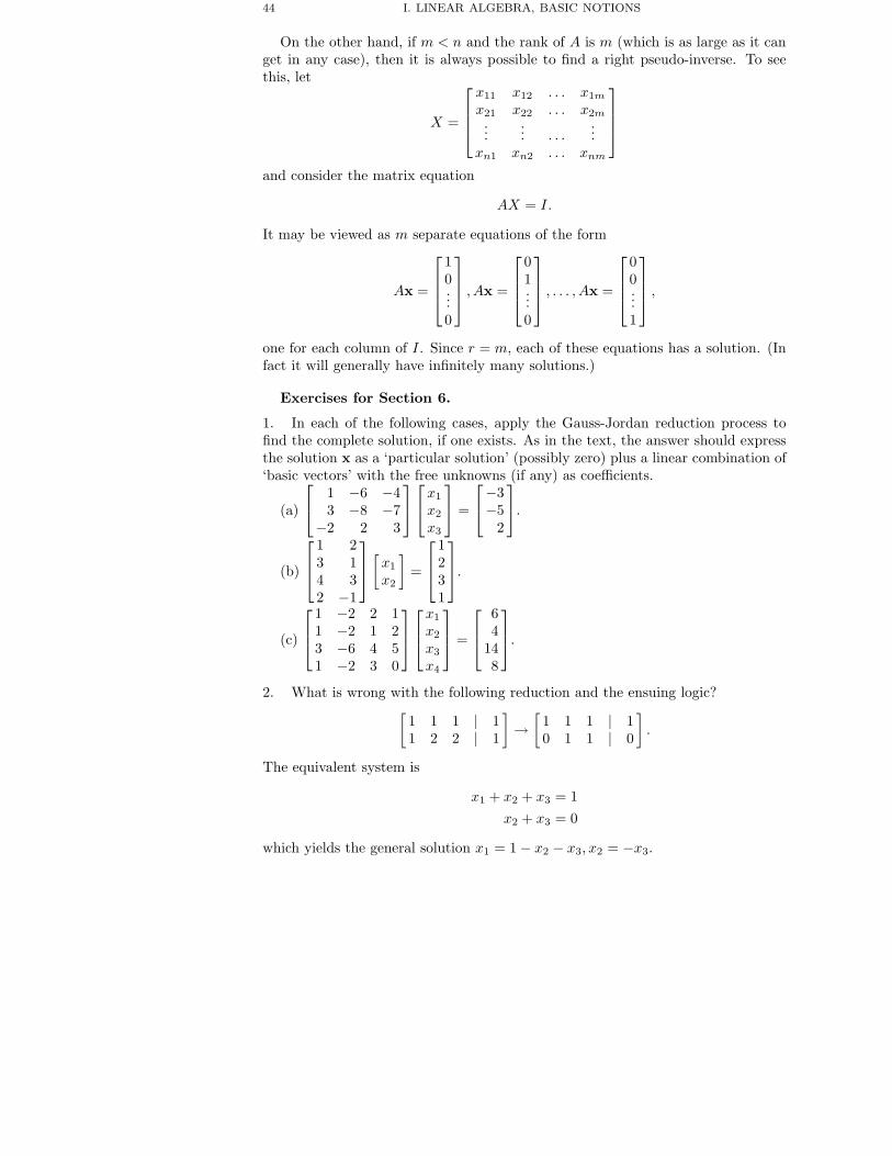
44 I. LINEAR ALGEBRA, BASIC NOTIONS
On the other hand, if m < n and the rank of A is m (which is as large as it canget in any case), then it is always possible to find a right pseudo-inverse. To seethis, let
X =
x11 x12 . . . x1m
x21 x22 . . . x2m...
... . . ....
xn1 xn2 . . . xnm
and consider the matrix equation
AX = I.
It may be viewed as m separate equations of the form
Ax =
10...0
, Ax =
01...0
, . . . , Ax =
00...1
,
one for each column of I. Since r = m, each of these equations has a solution. (Infact it will generally have infinitely many solutions.)
Exercises for Section 6.
1. In each of the following cases, apply the Gauss-Jordan reduction process tofind the complete solution, if one exists. As in the text, the answer should expressthe solution x as a ‘particular solution’ (possibly zero) plus a linear combination of‘basic vectors’ with the free unknowns (if any) as coefficients.
(a)
1 −6 −4
3 −8 −7−2 2 3
x1
x2
x3
=
−3−5
2
.
(b)
1 23 14 32 −1
[
x1
x2
]=
1231
.
(c)
1 −2 2 11 −2 1 23 −6 4 51 −2 3 0
x1
x2
x3
x4
=
64
148
.
2. What is wrong with the following reduction and the ensuing logic?[1 1 1 | 11 2 2 | 1
]→
[1 1 1 | 10 1 1 | 0
].
The equivalent system is
x1 + x2 + x3 = 1x2 + x3 = 0
which yields the general solution x1 = 1− x2 − x3, x2 = −x3.

6. GAUSS–JORDAN REDUCTION IN THE GENERAL CASE 45
3. Find a general solution vector of the system Ax = 0 where
(a) A =
1 0 1 2
2 −1 1 0−1 4 −1 −2
(b) A =
1 3 4 0 2
2 7 6 1 14 13 14 1 3
4. Consider the vectors
u =
−1
010
, v =
1101
in R4. If these were vectors in R3, we could use the formula
cos θ =u · v|u||v|
to determine the angle θ between the two vectors. In R4, we can’t of course talkdirectly about angles in the geometric sense we are familiar with, but we can stilluse the above formula to define the angle between the two vectors. In this example,find that angle.
5. What is the rank of the coefficient matrix for each of the matrices in theprevious problem.
6. What is the rank of each of the following matrices? 1 1 1
1 2 34 5 6
,
1 2 3 4
0 0 0 00 0 0 0
,
1234
7. Let A be an m × n matrix with m < n, and let r be its rank. Which of thefollowing is always true, sometimes true, never true?
(a) r ≤ m < n. (b) m < r < n. (c) r = m. (d) r = n. (e) r < m. (f) r = 0.
8. (a) A system Ax = b with A an m × n matrix of rank r will always havesolutions if m = r. Explain.
(b) It will not have solutions for some choices of b if r < m. Explain.
9. How do you think the rank of a product AB compares to the rank of A? Isthe former rank always ≤, ≥, or = the latter rank? Try some examples, make aconjecture, and see if you can prove it. Hint: Look at the number of rows of zeroesafter you reduce A completely to A′. Could further reduction transform A′B to amatrix with more rows of zeroes?
10. (Optional) Find a right pseudo-inverse A′ for
A =[
1 1 22 1 1
].
Note that there are infinitely many answers to this problem. You need only findone, but if you are ambitious, you can find all of them. Is there a left pseudo-inversefor A. If there is find one, if not explain why not.

46 I. LINEAR ALGEBRA, BASIC NOTIONS
11. (Optional) If A is an m × n matrix with m > n (more rows that columns),we showed in the text that there can be no right pseudo-inverse A′ for A. How canwe use this fact to conclude that if m < n (fewer rows than columns), there is noleft pseudo-inverse for A?
7. Homogeneous Systems and Vector Subspaces
As mentioned in the previous section, a system of equations of the form
Ax = 0
is called homogeneous. (The ‘b’ for such a system consists of zeroes.) A system ofthe form
Ax = b
where b 6= 0 is called inhomogeneous. Every inhomogeneous system has an associ-ated homogeneous system, and the solutions of the two systems are closely related.To see this, review the example from the previous section
1 1 2−1 −1 1
1 1 3
x1
x2
x3
=
1
53
.
We showed that its general solution has the form
(1) x =
−3
02
+ x2
−1
10
,
where x2 is free and may assume any value. On the other hand, it is easy to checkthat the homogeneous system
1 1 2−1 −1 1
1 1 3
x1
x2
x3
=
0
00
has the general solution
(2) x = x2
−1
10
,
where x2 is also free. (You should go back and verify that for yourself, which shouldbe easy since the Gauss-Jordan reduction is exactly the same; the only differenceis that you have zeroes to the right of the vertical bar.) A close reading of (1) and(2) is informative. First note that if we set x2 = 0 in (1), we obtain the specificsolution
−302

7. HOMOGENEOUS SYSTEMS AND VECTOR SUBSPACES 47
and then the remaining part of the solution is a general solution (2) of the homo-geneous equation.
The phenomenon illustrated above is part of a general principle. You can alwaysfind a general solution of an inhomogeneous linear system by adding one particularsolution to a general solution of the corresponding homogeneous system. The reasonfor this is fairly clear algebraically. Let x0 denote the particular solution of theinhomogeneous equation and let x denote any other solution. Then we have
Ax = b
Ax0 = b
which simply asserts that both are solutions. Now subtract
Ax−Ax0 = b− b = 0.
However, since Ax−Ax0 = A(x− x0), this yields
A(x− x0) = 0
from which we conclude that z = x− x0 is a solution of the homogeneous system.Transposition yields
x = x0︸︷︷︸par. sol.
+ z︸︷︷︸hom. sol.
.
Vector Subspaces. Because of the above remarks, homogeneous systems playa specially important role, so we want to concentrate on the solution sets of suchsystems. Let A be an m×n matrix. The set of all solutions x of the homogeneoussystem Ax = 0 is called the null space of A. Notice that the null space of an m×nmatrix is a subset of Rn.
Null spaces have an important property which we now discuss.A non-empty subset V of Rn is called a vector subspace if it has the property
that any linear combination of vectors in V is also in V . In symbols, if u and v arevectors in V , and a and b are scalars, then au + bv is also a vector in V .
In two and three dimensions, the subsets which are subspaces are pretty muchwhat you would expect. In R2 any line through the origin is a subspace, but linesnot through the origin are not. The diagram below indicates why.
O
Line not through origin Line through origin
O

48 I. LINEAR ALGEBRA, BASIC NOTIONS
Also, curves are not vector subspaces. (See the exercises at the end of the section).In R3 any line through the origin is also a subspace and lines not through the originare not. Similarly, planes through the origin are vector subspaces, but other planesare not, and of course curves or curved surfaces are not.
There is one slightly confusing point about the way we use this terminology.The entire set Rn is considered a subset of itself, and it certainly has the desiredproperty, so it is considered a vector subspace of itself.
It is not hard to see that the zero vector must be in every vector subspace W .Indeed, just pick any two vectors u and v in W—v could even be a multiple of u.Then 0 = (0)u + (0)v, the linear combination with both scalars a = b = 0, mustalso be in W . The upshot is that any set which does not contain the zero vectorcannot be a vector subspace.
The set consisting only of the zero vector 0 has the desired property—any linearcombination of zero with itself is also zero. Hence, that set is also a vector subspace,called the zero subspace.
The term ‘subspace’ is sometimes used more generally to refer to any subset ofRn. Hence the adjective ‘vector’ is crucial. Sometimes people use the term ‘linearsubspace’ instead.
There are two ways vector subspaces come about. First of all, as noted above,they arise as null spaces, i.e., as solution sets of homogeneous systems Ax = 0.That is the main reason we are interested in them. To see why a null space satisfiesthe definition, suppose u and v are both solutions of Ax = 0. That is, Au = 0 andAv = 0. Then
A(au + bv) = A(au) + A(bv) = aAu + bAv = a0 + b0 = 0.
So any linear combination of solutions is again a solution and is again in the nullspace of A.
There is another related way in which vector subspaces arise, and this will playan important role in analyzing solutions of linear systems. Recall the homogeneoussystem
(2)
1 2 −1 0
1 2 1 32 4 0 3
x1
x2
x3
x4
=
0
00
.
discussed in the previous section. We saw that its null space consists of all vectorsof the form
x2
−2
100
+ x4
−3/2
0−3/2
0
as the free scalars x2 and x4 range over all possible values. Let
v1 =
−2
100
v2 =
−3/2
0−3/2
0
.

7. HOMOGENEOUS SYSTEMS AND VECTOR SUBSPACES 49
Then, what we have discovered is that the solution set or null space consists ofall linear combinations of the set {v1,v2} of vectors. This is a much more usefulway of presenting the answer, since we specify it in terms of a small number ofobjects—in this case just two. Since the null space itself is infinite, this simplifiesthings considerably.
In general, suppose W is a vector subspace of Rn and {v1,v2, . . . ,vk} is a finitesubset of W . We say that {v1,v2, . . . ,vn} is a spanning set for W (or more simplythat it spans W ) if each vector v in W can be expressed as a linear combination
v = s1v1 + s2v2 + · · ·+ skvk,
for appropriate scalars s1, s2, . . . , sk. The simplest case of this is when k = 1, i.e.,the spanning set consists of a single vector v. Then the subspace spanned by thisvector is just the set of all sv with s an arbitrary scalar. If v 6= 0, this set is justthe line through the origin containing v.
Example. Consider the set of solutions x in R4 of the single homogeneousequation
x1 − x2 + x3 − 2x4 = 0.
This is the null space of the 1× 4 matrix
A = [ 1 −1 1 −2 ] .
The matrix is already reduced with pivot 1 in the 1, 1-position. The general solutionis
x1 = x2 − x3 + 2x4 x2, x3, x4 free,
and the general solution vector is
x =
x2 − x3 + 2x4
x2
x3
x4
= x2
1100
+ x3
−1
010
+ x4
2001
.
It follows that the null space is spanned by
v1 =
1100
, v2 =
−1
010
, v3 =
2001
.
This is a special case of a more general principle: Gauss-Jordan reduction for ahomogeneous system always results in a description of the null space as the vectorsubspace spanned by a finite set of basic solution vectors . We shall elaborate a bitmore on this principle in the next section.

50 I. LINEAR ALGEBRA, BASIC NOTIONS
Exercises for Section 7.
1. What is the general solution of the equation x1 − 2x2 + x3 = 4? Expressit as the sum of a particular solution plus the general solution of the equationx1 − 2x2 + x3 = 0.
2. Determine if each of the following subsets of R3 is a vector subspace of R3. Ifit is not a subspace, explain what fails.
(a) The set of all x =
x1
x2
x3
such that 2x1 − x2 + 4x3 = 0.
(b) The set of all x =
x1
x2
x3
such that 2x1 − x2 + 4x3 = 3.
(c) The set of all x =
x1
x2
x3
such that x1
2 + x22 − x3
2 = 1.
(d) The set of all x of the form x =
1 + 2t−3t2t
where t is allowed to assume any
real value.
(e) The set of all x of the form x =
s + 2t
2s− 3ts + 2t
where s and t are allowed to
assume any real values.
3. Let L1 and L2 be two distinct lines through the origin in R2. Is the set Sconsisting of all vectors pointing along one or the other of these two lines a vectorsubspace of R2?
4. Let
u1 =
1
10
and u2 =
0
13
.
What is the subspace of R3 spanned by these two vectors? Describe it another way.
5. (a) What is the subspace of R3 spanned by the set
v1 =
1
12
, v2 =
1
01
, v3 =
2
13
?
(b) What is the subspace of R3 spanned by
v1 =
0
11
, v2 =
1
12
, v3 =
1
23
?

8. LINEAR INDEPENDENCE, BASES, AND DIMENSION 51
6. (a) Find a spanning set for the plane in R3 through the origin defined by theequation x1 − 2x2 + 5x3 = 0. Check that each element of your spanning set isperpendicular to the normal vector with components 〈1,−2, 5〉.
(b) Find a spanning set for the line in R2 through the origin defined by theequation x1 + x2 = 0.
8. Linear Independence, Bases, and Dimension
Let V be a vector subspace of Rn. If V is not the zero subspace, it will haveinfinitely many elements, but it turns out that it is always possible to specify V asthe subspace spanned by some finite subset {v1,v2, . . . ,vk} of elements of V . (Ifyou are curious why, see the appendix to this section where it is proved.)
When doing this, we want to make sure that we don’t have any superfluousvectors in the set {v1,v2, . . . ,vk}.
Example 1. Let
v1 =
1
24
, v2 =
1
23
.
The subspace of R3 spanned by these two vectors is a plane through the origin.
Neither of these vectors is superfluous since if you omit either, what you get is theline through the origin containing the other. You don’t get the entire plane.
Consider instead the vectors
v1 =
1
24
, v2 =
2
48
.
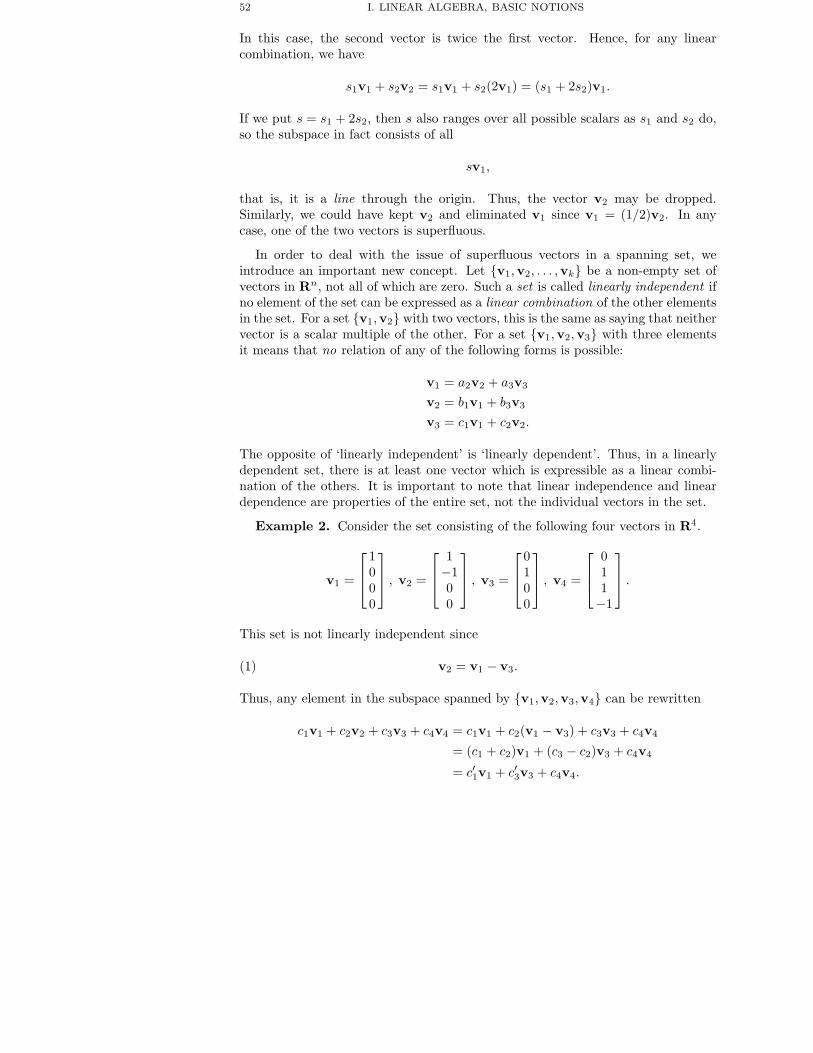
52 I. LINEAR ALGEBRA, BASIC NOTIONS
In this case, the second vector is twice the first vector. Hence, for any linearcombination, we have
s1v1 + s2v2 = s1v1 + s2(2v1) = (s1 + 2s2)v1.
If we put s = s1 + 2s2, then s also ranges over all possible scalars as s1 and s2 do,so the subspace in fact consists of all
sv1,
that is, it is a line through the origin. Thus, the vector v2 may be dropped.Similarly, we could have kept v2 and eliminated v1 since v1 = (1/2)v2. In anycase, one of the two vectors is superfluous.
In order to deal with the issue of superfluous vectors in a spanning set, weintroduce an important new concept. Let {v1,v2, . . . ,vk} be a non-empty set ofvectors in Rn, not all of which are zero. Such a set is called linearly independent ifno element of the set can be expressed as a linear combination of the other elementsin the set. For a set {v1,v2} with two vectors, this is the same as saying that neithervector is a scalar multiple of the other. For a set {v1,v2,v3} with three elementsit means that no relation of any of the following forms is possible:
v1 = a2v2 + a3v3
v2 = b1v1 + b3v3
v3 = c1v1 + c2v2.
The opposite of ‘linearly independent’ is ‘linearly dependent’. Thus, in a linearlydependent set, there is at least one vector which is expressible as a linear combi-nation of the others. It is important to note that linear independence and lineardependence are properties of the entire set, not the individual vectors in the set.
Example 2. Consider the set consisting of the following four vectors in R4.
v1 =
1000
, v2 =
1−100
, v3 =
0100
, v4 =
011−1
.
This set is not linearly independent since
(1) v2 = v1 − v3.
Thus, any element in the subspace spanned by {v1,v2,v3,v4} can be rewritten
c1v1 + c2v2 + c3v3 + c4v4 = c1v1 + c2(v1 − v3) + c3v3 + c4v4
= (c1 + c2)v1 + (c3 − c2)v3 + c4v4
= c′1v1 + c′3v3 + c4v4.

8. LINEAR INDEPENDENCE, BASES, AND DIMENSION 53
On the other hand, if we delete the element v2, the set consisting of the vectors
v1 =
1000
, v3 =
0100
, v4 =
011−1
.
is linearly independent. To see this, just look carefully at the pattern of zeroes.For example, v1 has first component 1, and the other two have first component 0,so v1 could not be a linear combination of v2 and v3. Similar arguments eliminatethe other two possible relations.
In the above example, we could just as well have written
v1 = v2 + v3
and eliminated v1 from the spanning set without loss. In general, there are manypossible ways to delete superfluous vectors from a spanning set.
There are a couple of slightly confusing points about the definition of linearindependence. First, the set {v} consisting of a single nonzero vector v is linearlyindependent . (For, there aren’t any other vectors in the set which could be linearcombinations of it.) The set {0} consisting only of the zero vector is not covered bythe definition, but, for technical reasons, we specify that it is linearly dependent .Also, for technical reasons, we specify that the empty set, that is, the set with novectors, is linearly independent.
Bases. Let V be a vector subspace of Rn. A subset {v1,v2, . . . ,vk} of V whichspans it and is also linearly independent is called a basis for V .
A simple example of a basis is the sete1 =
1
00
, e2 =
0
10
, e3 =
0
01
which is a basis for R3. (These vectors are usually called i, j, and k in threedimensional vector algebra. They are the unit vectors pointing along the coordinateaxes.) To see that this set is linearly independent, notice that the pattern of onesand zeroes precludes one of them being expressible as a linear combination of theothers. Each is one where the others are zero. To see that the set spans R3, notethat we can write any vector x in R3 as
x =
x1
x2
x3
=
x1
00
+
0
x2
0
+
0
0x3
= x1
1
00
+ x2
0
10
+ x3
0
01
= x1e1 + x2e2 + x3e3.
In general, let ei be the vector in Rn with all entries zero except the ith entrywhich is one. (One may also describe this vector as the ith column of the n × n
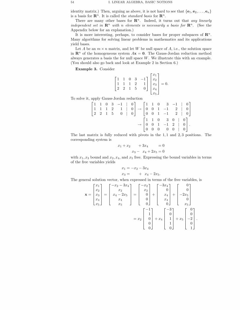
54 I. LINEAR ALGEBRA, BASIC NOTIONS
identity matrix.) Then, arguing as above, it is not hard to see that {e1, e2, . . . , en}is a basis for Rn. It is called the standard basis for Rn.
There are many other bases for Rn. Indeed, it turns out that any linearlyindependent set in Rn with n elements is necessarily a basis for Rn. (See theAppendix below for an explanation.)
It is more interesting, perhaps, to consider bases for proper subspaces of Rn.Many algorithms for solving linear problems in mathematics and its applicationsyield bases.
Let A be an m×n matrix, and let W be null space of A, i.e., the solution spacein Rn of the homogeneous system Ax = 0. The Gauss-Jordan reduction methodalways generates a basis the for null space W . We illustrate this with an example.(You should also go back and look at Example 2 in Section 6.)
Example 3. Consider
1 1 0 3 −1
1 1 1 2 12 2 1 5 0
x1
x2
x3
x4
x5
= 0.
To solve it, apply Gauss-Jordan reduction 1 1 0 3 −1 | 0
1 1 1 2 1 | 02 2 1 5 0 | 0
→
1 1 0 3 −1 | 0
0 0 1 −1 2 | 00 0 1 −1 2 | 0
→ 1 1 0 3 0 | 0
0 0 1 −1 2 | 00 0 0 0 0 | 0
.
The last matrix is fully reduced with pivots in the 1, 1 and 2, 3 positions. Thecorresponding system is
x1 + x2 + 3x4 = 0x3 − x4 + 2x5 = 0
with x1, x3 bound and x2, x4, and x5 free. Expressing the bound variables in termsof the free variables yields
x1 = −x2 − 3x4
x3 = + x4 − 2x5.
The general solution vector, when expressed in terms of the free variables, is
x =
x1
x2
x3
x4
x5
=
−x2 − 3x4
x2
x4 − 2x5
x4
x5
=
−x2
x2
000
+
−3x4
0x4
x4
0
+
00
−2x5
0x5
= x2
−1
1000
+ x4
−3
0110
+ x5
00
−201
.

8. LINEAR INDEPENDENCE, BASES, AND DIMENSION 55
If we put
v1 =
−1
1000
, v2 =
−3
0110
, v3 =
00
−201
,
and c1 = x2, c2 = x4, and c3 = x5, then the general solution takes the form
x = c1v1 + c2v2 + c3v3
where the scalars c1, c2, c3 (being new names for the free variables) can assumeany values. Also, the set {v1,v2,v3} is linearly independent. This is clear for thefollowing reason. Each vector is associated with one of the free variables and has a1 in that position where the other vectors necessarily have zeroes. Hence, none ofthe vectors can be linear combinations of the others. It follows that {v1,v2,v3} isa basis for the null space.
The above example illustrates all the important aspects of the solution processfor a homogeneous system
Ax = 0.
We state the important facts about the solution without going through the generalproofs since they are just the same as what we did in the example but with a lotmore confusing notation. The general solution has the form
x = s1v1 + s2v2 + · · ·+ skvk
where v1,v2, . . . ,vk are basic solutions obtained by successively setting each freevariable equal to 1 and the other free variables equal to zero. s1, s2 . . . , sk are justnew names for the free variables. The set {v1,v2, . . . ,vk} is linearly independentbecause of the pattern of ones and zeroes at the positions of the free variables, andsince it spans the null space, it is a basis for the null space of A.
The dimension of the null space of A is the nullity of A, i.e., it is the number offree variables in the solution of the homogeneous system Ax = 0.
There are some special cases which are a bit confusing. First, if k = 1, the basisconsists of a single vector v1, and the set of solutions consists of all multiples of thatvector. A much more confusing case is that in which the spanning set is the emptyset , i.e., the set with no elements. That would arise if the zero solution were theunique solution of the homogeneous system, so there would be no free variables andno basic solutions. This is dealt with as follows. First, as noted earlier, the emptyset is linearly independent by convention. Second, again by convention, every linearcombination of no vectors is set to zero. It follows that the empty set spans thezero subspace {0}, and is a basis for it.
Let V be a vector subspace of Rn. If V has a basis {v1,v2, . . . ,vk} with kelements, then we say that V is k-dimensional. That is, the dimension of a vectorsubspace is the number of elements in a basis.
Not too surprisingly, for the extreme case V = Rn, the dimension is n. For, thestandard basis {e1, e2, . . . , en} has n elements.

56 I. LINEAR ALGEBRA, BASIC NOTIONS
In this chapter we have defined the concept dimension only for vector subspacesor Rn, but the notion is considerably more general. For example, a plane in R3
should be considered two dimensional even if it doesn’t pass through the origin.Also, a surface in R3, e.g., a sphere or hyperboloid, should also be considered twodimensional. (People are often confused about curved objects because they seemto extend in extra dimensions. The point is that if you look at a small part ofa surface, it normally looks like a piece of a plane, so it has the same dimension.Also, a surface can usually be represented parametrically with only two parameters.)Mathematicians have developed a very general theory of dimension which applies toalmost any type of set. In cosmology, one envisions the entire universe as a certaintype of four dimensional object. Certain bizarre sets can even have a fractionaldimension, and that concept is useful in what is called ‘chaos’ theory.
Coordinates. Let V be a subspace of Rn and suppose {v1,v2, . . . ,vk} is abasis for V . Suppose v is any vector of V . Then
v = s1v1 + s2v2 + · · ·+ skvk
for appropriate coefficients s1, s2, . . . , sk. The coefficients s1, s2, . . . , sk in such alinear combination are unique, and are called the coordinates of the vector v withrespect to the basis. We illustrate this with an example which shows how to findcoordinates and why they are unique.
Example 4. Consider the plane V in R3 spanned by the linearly independentpair of vectors
v1 =
1
24
, v2 =
1
13
and consider the vector
v =
1
35
.
If v is in V , then it can be written
v = s1v1 + s2v2 = s1
1
24
+ s2
1
13
=
1
24
s1 +
1
13
s2.
Here, we have rewritten the linear combination with the scalars on the right. Theadvantage of so doing is that we may re-express it as a matrix product. Namely,
124
s1 +
1
13
s2 =
s1 + s2
2s1 + s2
4s1 + 3s2
=
1 1
2 14 3
[
s1
s2
].
Hence, asking if v = v1s1 + v2s2 amounts to asking if 1
35
=
1 1
2 14 3
[
s1
s2
]

8. LINEAR INDEPENDENCE, BASES, AND DIMENSION 57
has a solution s1, s2. This is a system of 3 equations in two unknowns (with the‘given’ vector on the left instead of as usual on the right). It may be solved byGauss-Jordan reduction as follows.
1 1 | 12 1 | 34 3 | 5
→
1 1 | 1
0 −1 | 10 −1 | 1
→
1 0 | 2
0 1 | −10 0 | 0
.
Thus, it has the unique solution s1 = 2, s2 = −1. Thus,[2
−1
]
is the coordinate vector giving the coordinates of v with respect to this basis, i.e.,v can be written uniquely
v = 2v1 − v2 = v1(2) + v2(−1) = [v1 v2 ][
2−1
].
.
There are a couple of points about the above example which merit some discus-sion. First, had the system not had a solution, that would just have meant thatthe vector v was not in fact in the subspace spanned by {v1,v2}. Second, thesolution was unique because the rank was as large as possible, in this case two,and there were no free variables. If the rank had been smaller than two, then thecorresponding homogeneous system
v1s1 + v2s2 = [v1 v2 ][
s1
s2
]= 0
would necessarily have had non-zero solutions. However, any such solution withsay s2 6= 0, would have allowed us to express
v2 = −v1s1
s2
which would contradict the linear independence of the basis.The general case is similar. If {v1,v2, . . . ,vk} is a basis for the subspace V of
Rn, then v is in this subspace if and only if the system
v = [v1 v2 . . . vk ]
s1
s2...
sk
has a solution. (Note that the ‘given’ vector v is on the left rather than on theright as usual.) The coefficient matrix [v1 v2 . . . vk ] is an n× k matrix withcolumns the elements of the basis. It is necessarily of largest possible rank k, and thesolution of the system is unique. Otherwise, the corresponding homogeneous system

58 I. LINEAR ALGEBRA, BASIC NOTIONS
would have non-trivial solutions and that would contradict the linear independenceof the basis.
Given a basis for a vector subspace V , one may think of the elements of the basisas unit vectors pointing along coordinate axes for V . The coordinates with respectto the basis then are the coordinates relative to these axes. The case V = Rn isspecially enlightening. Implicitly at least one starts in Rn with the standard basisconsisting of the vectors
e1 =
1
...0
, . . . , en =
0
...1
.
However, there are many other possible bases for Rn which might be useful insome applications. The axes associated with such a basis need not be mutuallyperpendicular, and also the units of length along these axes may differ.
Appendix. Some subtleties. We discuss here some of the subtleties of thetheory. This should be of interest to mathematics majors and some others whoenjoy theory, but it is not essential for understanding the subject matter.
First, we explain why any linearly independent subset {v1,v2, . . . ,vn} with ex-actly n elements is necessarily a basis for Rn. Namely, we saw that the linearindependence of the set assures us that the n× n matrix
[v1 v2 . . .vn ]
has rank n. Hence, it follows from our general theory that
v = [v1 v2 . . .vn ]
s1
s2...
sn
will have a solution
s1
s2...
sn
for every v in Rn. That is, every vector in Rn is expressible as a linear combinationof {v1,v2, . . . ,vn}.
Next, we investigate some subtle points involved in the definition of dimension.Invariance of dimension.The dimension of V is the number of elements in a basis for V , but it is at least
conceivable that two different bases have different numbers of elements. If thatwere the case, V would have two different dimensions, and that does not squarewith our idea of how such words should be used.
In fact it can never happen that two different bases have different numbers ofelements. To see this, we shall prove something slightly different. Suppose V has abasis with k elements. We shall show that

8. LINEAR INDEPENDENCE, BASES, AND DIMENSION 59
any linearly independent subset of V has at most k elements.This would suffice for what we want because if we had two bases one with k and
the other with m elements, either could play the role of the basis and the otherthe role of the linearly independent set. (Any basis is also linearly independent!)Hence, on the one hand we would have k ≤ m and on the other hand m ≤ k,whence it follows that m = k.
Here is the proof of the above assertion about linearly independent subsets.Let {u1,u2, . . . ,um} be a linearly independent subset. Each ui can be expressed
uniquely in terms of the basis
u1 =k∑
j=1
vjpj1 = [v1 v2 . . . vk ]
p11
p21...
pk1
u2 =k∑
j=1
vjpj2 = [v1 v2 . . . vk ]
p21
p22...
pk2
...
um =k∑
j=1
vjpjm = [v1 v2 . . . vk ]
p1m
p2k...
pkm
.
Each of these equations represents one column of the complete matrix equation
[u1 u2 . . . um ] = [v1 v2 . . . vk ]
p11 p12 . . . p1m
p21 p22 . . . p2m...
... . . ....
pk1 pk2 . . . pkm
.
Note that the matrix on the right is an k ×m matrix. Consider the homogeneoussystem
p11 p12 . . . p1m
p21 p22 . . . p2m...
... . . ....
pk1 pk2 . . . pkm
x1
x2...
xm
= 0.
Assume, contrary to what we hope, that m > k. Then, we know by the theory ofhomogeneous linear systems, that there is a non-trivial solution to this system, i.e.,

60 I. LINEAR ALGEBRA, BASIC NOTIONS
one with at least one xi not zero. Then
[u1 u2 . . . um ]
x1
x2...
xm
=
[v1 v2 . . . vk ]
p11 p12 . . . p1m
p21 p22 . . . p2m...
... . . ....
pk1 pk2 . . . pkm
x1
x2...
xm
= 0.
Thus, 0 has a non-trivial representation
0 = u1x1 + u2x2 + · · ·+ umxm
which we know can never happen for a linearly independent set. Thus, the onlyway out of this contradiction is to believe that m ≤ k as claimed.
One consequence of this argument is the following fact. If V and W are subspacesof Rn with V ⊆ W , then the dimension of V is less than or equal to the dimensionof W , i.e., larger subspaces have larger dimension. The reasoning is that a basisfor V is necessarily a linearly independent set and so it cannot have more elementsthan the dimension of W .
It is important to note that two different bases of the same vector space mighthave no elements whatsoever in common. All we can be sure of is that they havethe same size.
Existence of Bases.We assumed implicitly in our discussion of subspaces that every subspace V does
in fact have a basis. The following arguments show that this is true.Start by choosing a sequence of vectors v1,v2,v3, . . . in V , but make sure that
at each stage the next vector vp that you choose is not a linear combination ofthe previous vectors v1,v2, . . . ,vp−1. It is possible to show that the finite set{v1,v2, . . . ,vp} is always linearly independent. (The vector vp is not a linearcombination of the others by construction, but you have to fiddle a bit to show thenone of the previous ones are linear combinations involving vp.) The only questionthen is whether or not this sequence can go on forever. It can’t do that sinceeventually we would get a linearly independent subset of Rn with n + 1 elements,and since Rn has dimension n, that is impossible. Hence, the sequence stops, since,at some stage, we can’t choose any vector in V which is not a linear combinationof the set of vectors so far chosen. Thus, that set spans V , and since, as just noted,it is linearly independent, it is a basis.
Exercises for Section 8.
1. In each of the following cases, determine if the indicated set is linearly inde-pendent or not.

8. LINEAR INDEPENDENCE, BASES, AND DIMENSION 61
(a)
1
23
,
0
11
,
1
12
.
(b)
1001
,
0101
,
0011
.
2. Find a basis for the subspace of R4 consisting of solutions of the homogeneoussystem
1 −1 1 −11 2 −1 10 3 −2 2
x = 0.
3. Find the dimension of the nullspace of A in each of the following cases. (Seethe Exercises for Section 6.)
(a) A =
1 0 1 2
2 −1 1 0−1 4 −1 −2
(b) A =
1 3 4 0 2
2 7 6 1 14 13 14 1 3
4. Can the zero vector be an element of a linearly independent set?
5. (Optional) Let {v1,v2,v3} be a subset of Rn Show that the set is linearlyindependent if and only if the equation
0 = c1v2 + c2v2 + c3v3
has only the trivial solution, i.e., all the coefficients c1 = c2 = c3 = 0.The generalization of this to n vectors is very convenient to use when proving a
set is linearly independent. It is often taken as the definition of linear independencein books on linear algebra.
6. Let
v1 =
1
10
, v2 =
0
11
, v3 =
1
01
.
(a) Show that {v1,v2,v3} is a linearly independent set. Hint. If one of the threevectors were a linear combination of the other two, what relation would it have tothe cross product of those two?
(b) Why can you conclude that it is a basis for R3?
(c) Find the coordinates of v =
1
12
with respect to this basis.
7. Show that
u1 =[
1−1
]and u2 =
[11
]

62 I. LINEAR ALGEBRA, BASIC NOTIONS
form a linearly independent pair in R2. It follows that they form a basis for R2.Why? Find the coordinates of e1 and e2 with respect to this new basis. Hint. Youneed to solve
[u1 u2 ][
x1
x2
]= e1 and [u1 u2 ]
[x1
x2
]= e2.
You can solve these simultaneously by solving
[u1 u2 ]X = I
for an appropriate 2× 2 matrix X. What does this have to do with inverses?
8. Let
v1 =
1
10
, v2 =
0
11
.
(a) Show that {v1,v2} is a basis for the subspace W of R3 that it spans.
(b) Is v =
1−1−2
in this subspace? If so, find its coordinates with respect to
the basis.
9. (Optional) It is possible to consider infinite sequences of the form
x = (x1, x2, . . . , xn, . . . )
to be ‘infinite dimensional’ vectors. The set R∞ of all of these is a generalizationof a vector space, and many of the concepts we developed for Rn apply to it. Suchsequences are added by adding corresponding entries and a sequence is multipliedby a scalar by multiplying each entry by that scalar. Let ei be the vector in R∞
with xi = 1 and all other entries zero.(a) Show that the set {e1, e2, . . . , en} of the first n of these is a linearly inde-
pendent set for each n. Thus there is no upper bound on the size of a linearlyindependent subset of R∞.
(b) Does the set of all possible ei span R∞? Explain.
9. Calculations in Rn
Let {v1,v2, . . . ,vk} be a collection of vectors in Rn. It is a consequence of ourdiscussion of coordinates in the previous section that the set is linearly independentif and only if the n × k matrix [v1 v2 . . .vk ] has rank k. In that case, the setis a basis for the subspace W that is spans.

9. CALCULATIONS IN Rn 63
Example 1. Is
1
10
,
0
11
,
1
01
a linearly independent set? To test this, find the rank of the matrix with thesevectors as columns:
1 0 11 1 00 1 1
→
1 0 1
0 1 −10 1 1
→
1 0 1
0 1 −10 0 2
.
It is clear without proceeding further that the rank is three, so the set is linearlyindependent.
More generally, suppose {v1,v2, . . . ,vk} is a set of vectors in Rn which mayor may not be linearly independent. It is often useful to have a way to pick outa linearly independent subset of the set which spans the same subspace W as theoriginal set. Then that subset will be a basis for W . The basic idea (no punintended) is to throw away superfluous vectors until that is no longer possible, butthere is a systematic way to do this all at once. Since the vectors vi are elementsof Rn, each may be specified as a n× 1 column vector. Put these vectors togetherto form an n× k matrix
A = [v1 v2 . . . vk ] .
To find a basis, apply Gaussian reduction to the matrix A, and pick out the columnsof A which in the transformed reduced matrix end up with pivots.
Example 2. Let
v1 =
1011
, v2 =
2240
, v3 =
−1
10
−2
, v4 =
0110
.
Form the matrix A with these columns and apply Gaussian reduction
1 2 −1 00 2 1 11 4 0 11 0 −2 0
→
1 2 −1 10 2 1 10 2 1 10 −2 −1 0
→
1 2 −1 10 2 1 10 0 0 00 0 0 1
→
1 2 −1 10 2 1 10 0 0 10 0 0 0
.

64 I. LINEAR ALGEBRA, BASIC NOTIONS
This completes the Gaussian reduction, and the pivots are in the first, second, andfourth columns. Hence, the vectors
v1 =
1011
, v2 =
2240
, v4 =
0110
form a basis for the subspace spanned by {v1,v2,v3,v4}.Let’s look more closely at this example to see why the subset is linearly inde-
pendent and also spans the same subspace as the original set. The proof that thealgorithm works in the general case is more complicated to write down but justelaborates the ideas exhibited in the example. Consider the homogeneous systemAx = 0. This may also be written
Ax = [v1 v2 v3 v4 ]
x1
x2
x3
x4
= v1x1 + v2x2 + v3x3 + v4x4 = 0.
In the general solution, x1, x2, and x4 will be bound variables (from the pivotpositions) and x3 will be free. That means we can set x3 equal to anything, sayx3 = −1 and the other variables will be determined. For this choice, the relationbecomes
v1x1 + v2x2 − v3 + v4x4 = 0
which may be rewritten
v3 = x1v1 + x2v2 + x4v4.
Thus, v3 is superfluous and may be eliminated from the set without changing thesubspace spanned by the set. On the other hand, the set {v1,v2,v4} is linearlyindependent, since if we were to apply Gaussian reduction to the matrix
A′ = [v1 v2 v4 ]
the reduced matrix would have a pivot in every column, i.e., it would have rank 3.Thus, the system
[v1 v2 v4 ]
x1
x2
x4
= v1x1 + v2x2 + v4x4 = 0
has only the trivial solution. That means that no one of the three vectors can beexpressed as a linear combination of the other two. For example, if v2 = c1v1+c4v4,we have
v1c1 + v2(−1) + v4c4 = 0.
It follows that the set is linearly independent.

9. CALCULATIONS IN Rn 65
Column Space and Row Space. Let A be an m × n matrix. The columnsv1,v2, . . . ,vn of A are vectors in Rm, and {v1,v2, . . . ,vn} spans a subspace of Rm
called the column space of A. The column space plays a role in the the theory ofinhomogeneous systems Ax = b in the following way. A vector b is in the columnspace if and only if it is expressible as a linear combination
b = v1x1 + v2x2 + · · ·+ vnxn = [v1 v2 . . . vn ]
x1
x2...
xn
= Ax.
Thus, the column space of A consists of all vectors b in Rm for which the systemAx = b has a solution.
Example 3, continued. We wish to determine if
b =
1010
is in the column space of
A =
1 2 −1 00 2 1 11 4 0 11 0 −2 0
.
This will be true if and only if
A =
1 2 −1 00 2 1 11 4 0 11 0 −2 0
x =
1010
has a solution. Reduce the augmented matrix
1 2 −1 0 | 10 2 1 1 | 01 4 0 1 | 11 0 −2 0 | 0
→
1 2 −1 1 | 10 2 1 1 | 00 2 1 1 | 00 −2 −1 0 | −1
→
1 2 −1 1 | 10 2 1 1 | 00 0 0 0 | 00 0 0 1 | −1
→
1 2 −1 1 | 10 2 1 1 | 00 0 0 1 | −10 0 0 0 | 0
.

66 I. LINEAR ALGEBRA, BASIC NOTIONS
It is clear at this point that the system will have a solution, so we need not go anyfarther. We can conclude that b is in the column space of A.
Note that the method outlined in the beginning of this section gives a basisfor the column space, and the number of elements in this basis is the rank of A.(The rank is the number of pivots!) Hence, the rank of an m × n matrix A is thedimension of its column space.
The column space of a matrix A is often called the range of A. That is becauseit describes all possible vectors in Rm of the form Ax.
There is a similar concept for rows; the row space of an m × n matrix A is thesubspace of Rn spanned by the rows of A. It is not hard to see that the dimensionof the row space of A is also the rank of A. For, since each row operation isreversible, applying a row operation does not change the subspace spanned by therows. Hence, the row space of the matrix A′ obtained by Gauss-Jordan reductionfrom A is the same as the row space of A. However, the set of non-zero rows of thereduced matrix is a basis for this subspace. To see this, note first that it certainlyspans (since leaving out zero rows doesn’t cost us anything). Moreover, it is alsoa linearly independent set because each non-zero row has a 1 in a pivot positionwhere all the other rows are zero.
The fact that both the column space and the row space have the same dimensionis sometimes expressed by saying “the column rank equals the row rank”. Of course,there is no particular reason why the row space and the column space should beidentical. For example, unless the matrix is square, the vectors in them won’t evenhave the same number of components.
A Note on the Definition of Rank. The rank of A is defined as the numberof pivots in the reduced matrix obtained from A by an appropriate sequence of ele-mentary row operations. Since we can specify a standard procedure for performingsuch row operations, that means the rank is a well defined number. On the otherhand, it is natural to wonder what might happen if A were reduced by an alter-native, perhaps less systematic, sequence of row operations. The above analysisshows that we would still get the same answer for the rank. Namely, the rank isthe dimension of the column space of A, and that number depends only on thecolumn space itself, not on any particular basis for it. (Or you could use the sameargument using the row space.)
The rank is also the number of non-zero rows in the reduced matrix, so it followsthat this number does not depend on the particular sequence of row operations usedto reduce A to Gauss-Jordan reduced form. In fact, the entire matrix obtained atthe end (as long as it is in Gauss-Jordan reduced form) depends only on the originalmatrix A and not on the particular sequence or row operations used to obtain it.The proof of this fact is not so easy, and we omit it here.
Exercises for Section 9.
1. Find a subset of the following set of vectors which is a basis for the subspace

10. REVIEW PROBLEMS 67
it spans.
1230
,
30
−32
,
3331
,
1−1−3
1
2. Let A =
1 0 2 1 1−1 1 3 0 1
1 1 7 2 3
.
(a) Find a basis for the column space of A.(b) Find a basis for the row space of A.
3. Let
v1 =
1−2−1
, v2 =
1
21
.
Find a basis for R3 by finding a third vector v3 such that {v1,v2,v3} is linearlyindependent. Hint. You may find an easier way to do it, but the following methodshould work. Use the method suggested in Section 9 to pick out a linearly inde-pendent subset from {v1,v2, e1, e2, e3}.
4. (Optional) Let {v1,v2, . . . ,vk} be a linearly independent subset of Rn. Applythe method in section 9 to the set {v1,v2, . . . ,vk, e1, e2, . . . , en}. It will necessarilyyield a basis for Rn. Why? Show that this basis will include {v1,v2, . . . ,vk} as asubset. That is show that none of the vi will be eliminated by the process.
5. (a) Find a basis for the column space of
A =
1 2 2 3
1 2 3 43 6 7 10
.
(b) Is b =
0
11
in the column space of A?
6. (a) Suppose A is a 7 × 12 matrix and W is its range or column space. IfdimW = 7, what can you say about the general solvability of systems of the formAx = b?
(b) Suppose instead that A is 12 × 7. What if anything can you say about thegeneral solvability of systems of the form Ax = b?
10. Review Problems

68 I. LINEAR ALGEBRA, BASIC NOTIONS
Exercises for Section 10.
1. Find A−1 for A =
1 0 0−1 2 0
3 1 −1
. Check your answer by computing AA−1.
2. Let A =
2 −1 6 1 2
1 3 4 0 04 5 14 1 2
.
(a) Find the dimension of the nullspace of A.(b) Find the dimension of the column space of A.(c) How are these two numbers related?
3. What is wrong with the following statement? If A and B are invertible n× nmatrices, then AB is invertible and (AB)−1 = A−1B−1.
4. Suppose A is a 15×23 matrix. In which circumstances will each of the followingstatements be true?
(a) A system Ax = b of 15 equations in 23 unknowns has a solution for every bin R15.
(b) The homogeneous system Ax = 0 has infinitely many solutions.
5. Let A =
1 3 4 0 2
2 7 6 1 14 13 14 1 3
.
(a) Find a basis for the nullspace of the A.(b) Find the dimensions of the nullspace and the column space of A.
(c) Does
1
1−1
belong to the column space of A? Explain.
6. Find the inverse of A =
1 3 3
2 6 80 2 2
.
7. Let A =
1 2 2 3
1 2 3 43 6 7 10
.
(a) Find a basis for the nullspace of A.(b) Find a basis for the column space of A.(c) Do the columns of A form a linearly independent set? Explain.
(d) Does
2
34
belong to the column space of A? Explain your answer.
8. In each case tell if the indicated subset is a vector subspace of R3 and give areason for your answer.
(a) The plane defined by the equation x1 − 2x2 + 3x3 = 0.(b) The sphere defined by the equation x1
2 + x22 + x3
2 = 16.

10. REVIEW PROBLEMS 69
9. All the parts of this question refer to the matrix A =
1 2 1 3 1
2 1 3 3 21 −1 2 0 1
.
(a) What is the rank of A?(b) What is the dimension of the nullspace of A?
10. Consider the subset
1001
,
3110
,
1100
,
1000
of R4.(a) Is this set linearly independent? Explain?(b) Is it a basis for R4? Explain.

70 I. LINEAR ALGEBRA, BASIC NOTIONS